an introduction to bioinformatics 2. comparing biological sequences: sequence alignment (cont’d)

An Introduction to Bioinformatics

2. Comparing biological sequences:

sequence alignment (cont’d)


Outline

• Global Alignment • Scoring Matrices• Local Alignment• Alignment with Affine Gap Penalties


From LCS to Alignment: Change up the Scoring

• The Longest Common Subsequence (LCS) problem—the simplest form of sequence alignment – allows only insertions and deletions (no mismatches).

• In the LCS Problem, we scored 1 for matches and 0 for indels• Consider penalizing indels and mismatches with negative

scores• Simplest scoring schema: +1 : match premium -μ : mismatch penalty -σ : indel penalty


Simple Scoring

• When mismatches are penalized by –μ, indels are penalized by –σ,

and matches are rewarded with +1,

the resulting score is:

#matches – μ(#mismatches) – σ (#indels)


The Global Alignment ProblemFind the best alignment between two strings under a given

scoring schema

Input : Strings v and w and a scoring schemaOutput : Alignment of maximum score

↑→ = -б = 1 if match = -µ if mismatch

si-1,j-1 +1 if vi = wj

si,j = max s i-1,j-1 -µ if vi ≠ wj

s i-1,j - σ s i,j-1 - σ

: mismatch penaltyσ : indel penalty


Scoring Matrices

To generalize scoring, consider a (4+1) x(4+1) scoring matrix δ.

In the case of an amino acid sequence alignment, the scoring matrix would be a (20+1)x(20+1) size. The addition of 1 is to include the score for comparison of a gap character “-”.

This will simplify the algorithm as follows:

si-1,j-1 + δ (vi, wj)

si,j = max s i-1,j + δ (vi, -)

s i,j-1 + δ (-, wj)


Measuring Similarity

• Measuring the extent of similarity between two sequences• Based on percent sequence identity• Based on conservation


Percent Sequence Identity

• The extent to which two nucleotide or amino acid sequences are invariant

A C C T G A G – A G A C G T G – G C A G

70% identical

mismatchindel


Making a Scoring Matrix

• Scoring matrices are created based on biological evidence.

• Alignments can be thought of as two sequences that differ due to mutations.

• Some of these mutations have little effect on the protein’s function, therefore some penalties, δ(vi , wj), will be less harsh than others.


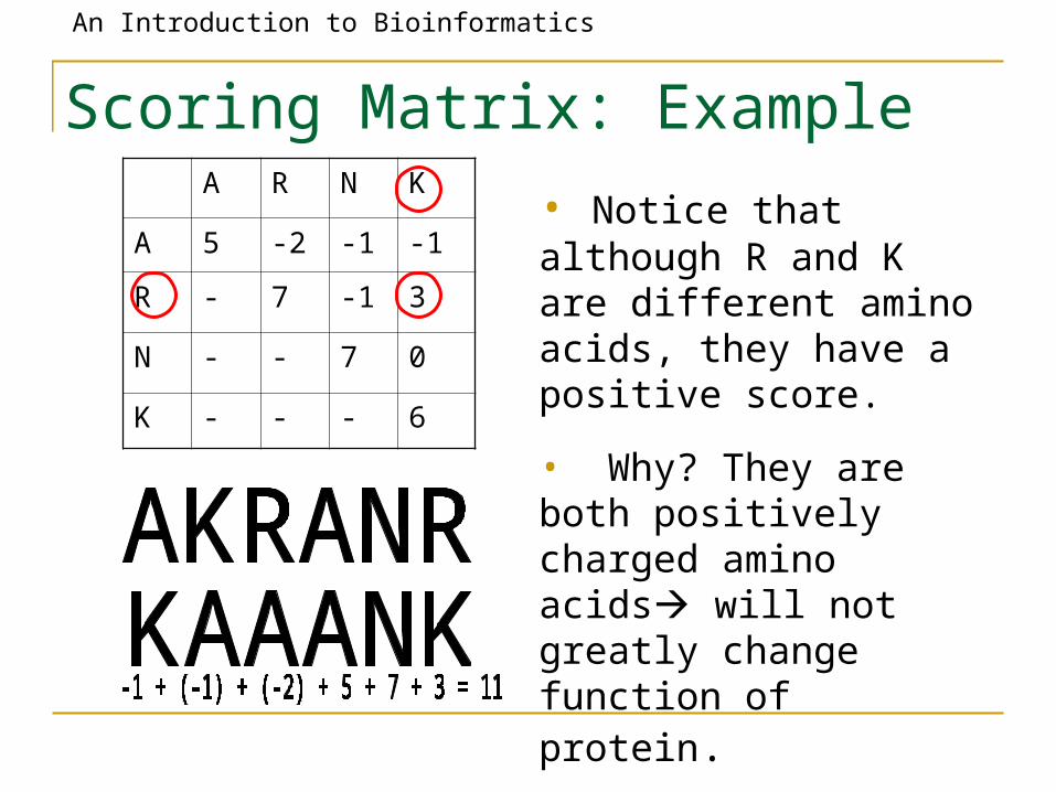
Scoring Matrix: ExampleA R N K

A 5 -2 -1 -1

R - 7 -1 3

N - - 7 0

K - - - 6

• Notice that although R and K are different amino acids, they have a positive score.

• Why? They are both positively charged amino acids will not greatly change function of protein.


Conservation

• Amino acid changes that tend to preserve the physico-chemical properties of the original residue• Polar to polar

• aspartate glutamate• Nonpolar to nonpolar

• alanine valine• Similarly behaving residues

• leucine to isoleucine


Scoring matrices

• Amino acid substitution matrices• PAM• BLOSUM

• DNA substitution matrices• DNA is less conserved than protein

sequences• Less effective to compare coding regions at

nucleotide level


PAM• Point Accepted Mutation (Dayhoff et al.)• 1 PAM = PAM1 = 1% average change of all amino

acid positions• After 100 PAMs of evolution, not every residue will

have changed• some residues may have mutated several

times• some residues may have returned to their

original state• some residues may not changed at all


PAMX

• PAMx = PAM1x

• PAM250 = PAM1250

• PAM250 is a widely used scoring matrix:

Ala Arg Asn Asp Cys Gln Glu Gly His Ile Leu Lys ... A R N D C Q E G H I L K ...Ala A 13 6 9 9 5 8 9 12 6 8 6 7 ...Arg R 3 17 4 3 2 5 3 2 6 3 2 9Asn N 4 4 6 7 2 5 6 4 6 3 2 5Asp D 5 4 8 11 1 7 10 5 6 3 2 5Cys C 2 1 1 1 52 1 1 2 2 2 1 1Gln Q 3 5 5 6 1 10 7 3 7 2 3 5...Trp W 0 2 0 0 0 0 0 0 1 0 1 0Tyr Y 1 1 2 1 3 1 1 1 3 2 2 1Val V 7 4 4 4 4 4 4 4 5 4 15 10


BLOSUM

• Blocks Substitution Matrix • Scores derived from observations of the

frequencies of substitutions in blocks of local alignments in related proteins

• Matrix name indicates evolutionary distance• BLOSUM62 was created using sequences

sharing no more than 62% identity


The Blosum50 Scoring Matrix


Local vs. Global Alignment

• The Global Alignment Problem tries to find the longest path between vertices (0,0) and (n,m) in the edit graph.

• The Local Alignment Problem tries to find the longest path among paths between arbitrary vertices (i,j) and (i’, j’) in the edit graph.


Local vs. Global Alignment• The Global Alignment Problem tries to find the

longest path between vertices (0,0) and (n,m) in the edit graph.

• The Local Alignment Problem tries to find the longest path among paths between arbitrary vertices (i,j) and (i’, j’) in the edit graph.

• In the edit graph with negatively-scored edges, Local Alignmet may score higher than Global Alignment


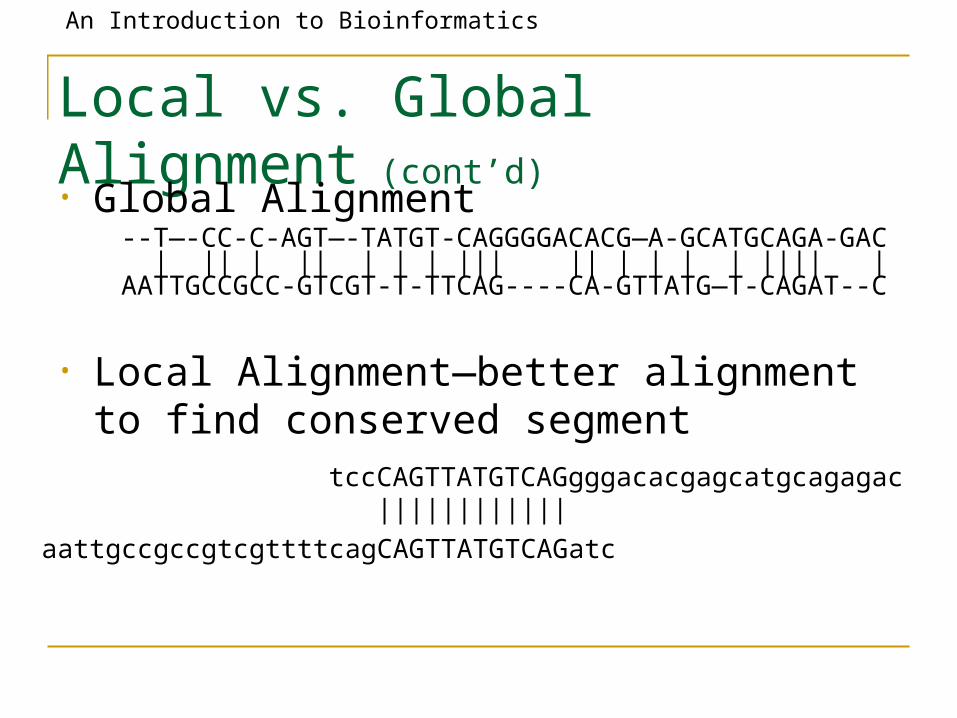
Local vs. Global Alignment (cont’d)• Global Alignment

• Local Alignment—better alignment to find conserved segment

--T—-CC-C-AGT—-TATGT-CAGGGGACACG—A-GCATGCAGA-GAC | || | || | | | ||| || | | | | |||| | AATTGCCGCC-GTCGT-T-TTCAG----CA-GTTATG—T-CAGAT--C

tccCAGTTATGTCAGgggacacgagcatgcagagac ||||||||||||

aattgccgccgtcgttttcagCAGTTATGTCAGatc


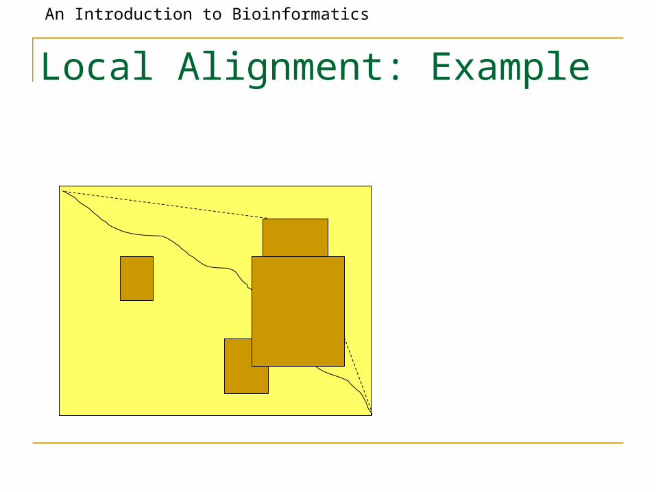
Local Alignment: Example

Global alignment

Local alignment

Compute a “mini” Global Alignment to get Local


Local Alignments: Why?• Two genes in different species may be similar over

short conserved regions and dissimilar over remaining regions.

• Example:• Homeobox genes have a short region called the

homeodomain that is highly conserved between species.

• A global alignment would not find the homeodomain because it would try to align the ENTIRE sequence


The Local Alignment Problem

• Goal: Find the best local alignment between two strings

• Input : Strings v, w and scoring matrix δ• Output : Alignment of substrings of v and w

whose alignment score is maximum among all possible alignment of all possible substrings


The Problem with this Problem• Long run time O(n4):

- In the grid of size n x n there are ~n2 vertices (i,j) that may serve as a source.

- For each such vertex computing alignments from (i,j) to (i’,j’) takes O(n2) time.

• This can be remedied by giving free rides



Global alignment

Local alignment

Compute a “mini” Global Alignment to get Local


Local Alignment: Running Time • Long run time O(n4):

- In the grid of size n x n there are ~n2 vertices (i,j) that may serve as a source.

- For each such vertex computing alignments from (i,j) to (i’,j’) takes O(n2) time.

• This can be remedied by giving free rides


Local Alignment: Free Rides

Vertex (0,0)

The dashed edges represent the free rides from (0,0) to every other node.

Yeah, a free ride!


The Local Alignment Recurrence

• The largest value of si,j over the whole edit graph is the score of the best local alignment.

• The recurrence:

0 si,j = max si-1,j-1 + δ (vi, wj)

s i-1,j + δ (vi, -)

s i,j-1 + δ (-, wj)

Notice there is only this change from the original recurrence of a Global Alignment


The Local Alignment Recurrence

• The largest value of si,j over the whole edit graph is the score of the best local alignment.

• The recurrence:

0 si,j = max si-1,j-1 + δ (vi, wj)

s i-1,j + δ (vi, -)

s i,j-1 + δ (-, wj)

Power of ZERO: there is only this change from the original recurrence of a Global Alignment - since there is only one “free ride” edge entering into every vertex


The Smith-Waterman algorithm

Idea: Ignore badly aligning regions

Modifications to Needleman-Wunsch:

Initialization: F(0, j) = F(i, 0) = 0

0

Iteration: F(i, j) = max F(i – 1, j) – d

F(i, j – 1) – d

F(i – 1, j – 1) + s(xi, yj)


Scoring Indels: Naive Approach

• A fixed penalty σ is given to every indel:• -σ for 1 indel, • -2σ for 2 consecutive indels• -3σ for 3 consecutive indels, etc.

Can be too severe penalty for a series of 100 consecutive indels


Affine Gap Penalties

• In nature, a series of k indels often come as a single event rather than a series of k single nucleotide events:

Normal scoring would give the same score for both alignments

This is more likely.

This is less likely.


Accounting for Gaps• Gaps- contiguous sequence of spaces in one of the

rows

• Score for a gap of length x is: -(ρ + σx) where ρ >0 is the penalty for introducing a gap: gap opening penalty ρ will be large relative to σ: gap extension penalty because you do not want to add too much of a

penalty for extending the gap.


Affine Gap Penalties

• Gap penalties:• -ρ-σ when there is 1 indel• -ρ-2σ when there are 2 indels• -ρ-3σ when there are 3 indels, etc. • -ρ- x·σ (-gap opening - x gap extensions)

• Somehow reduced penalties (as compared to naïve scoring) are given to runs of horizontal and vertical edges


Compromise: affine gaps

ρσ

Gap cost


Affine Gap Penalties and Edit Graph

To reflect affine gap penalties we have to add “long” horizontal and vertical edges to the edit graph. Each such edge of length x should have weight

- - x *


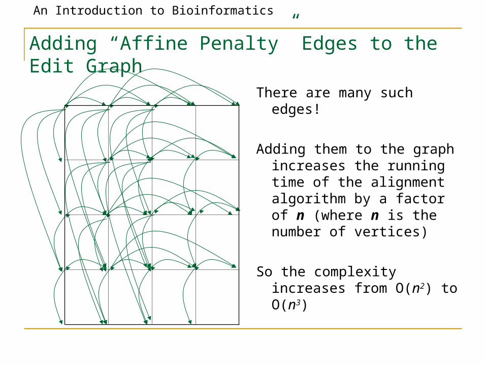
Adding “Affine Penalty” Edges to the Edit Graph

There are many such edges!

Adding them to the graph increases the running time of the alignment algorithm by a factor of n (where n is the number of vertices)

So the complexity increases from O(n2) to O(n3)


Manhattan in 3 Layers

ρ

ρ

σ

σδ

δ

δ

δδ


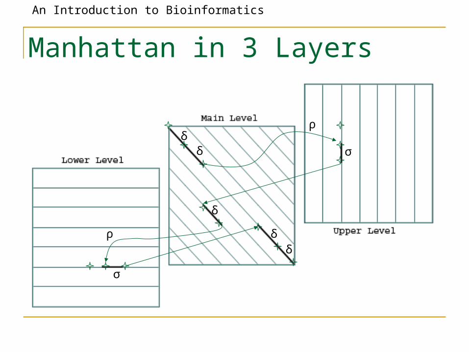
Affine Gap Penalties and 3 Layer Manhattan Grid

• The three recurrences for the scoring algorithm creates a 3-layered graph.

• The top level creates/extends gaps in the sequence w.

• The bottom level creates/extends gaps in sequence v.

• The middle level extends matches and mismatches.


Switching between 3 Layers

• Levels:• The main level is for diagonal edges • The lower level is for horizontal edges• The upper level is for vertical edges

• A jumping penalty is assigned to moving from the main level to either the upper level or the lower level (-)

• There is a gap extension penalty for each continuation on a level other than the main level (-)


The 3-leveled Manhattan Grid


Affine Gap Penalty Recurrencessi,j = s i-1,j - σ

max s i-1,j –(ρ+σ)

si,j = s i,j-1 - σ

max s i,j-1 –(ρ+σ)

si,j = si-1,j-1 + δ (vi, wj)

max s i,j

s i,j

Continue Gap in w (deletion)

Start Gap in w (deletion): from middle

Continue Gap in v (insertion)

Start Gap in v (insertion):from middle

Match or Mismatch

End deletion: from top

End insertion: from bottom


Bounded Dynamic ProgrammingInitialization:

F(i,0), F(0,j) undefined for i, j > k

Iteration:

For i = 1…M

For j = max(1, i – k)…min(N, i+k)

F(i – 1, j – 1)+ s(xi, yj)

F(i, j) = max F(i, j – 1) – d, if j > i – k(N)

F(i – 1, j) – d, if j < i + k(N)

Termination: same

Easy to extend to the affine gap case

x1 ………………………… xM

y1 …

……

……

……

……

…

yN

k(N)


Computing Alignment Path Requires Quadratic Memory

Alignment Path• Space complexity for

computing alignment path for sequences of length n and m is O(nm)

• We need to keep all backtracking references in memory to reconstruct the path (backtracking)

n

m


Computing Alignment Score with Linear MemoryAlignment Score• Space complexity of

computing just the score itself is O(n)

• We only need the previous column to calculate the current column, and we can then throw away that previous column once we’re done using it

2

nn


Computing Alignment Score: Recycling Columns

memory for column 1 is used to calculate column 3

memory for column 2 is used to calculate column 4

Only two columns of scores are saved at any given time


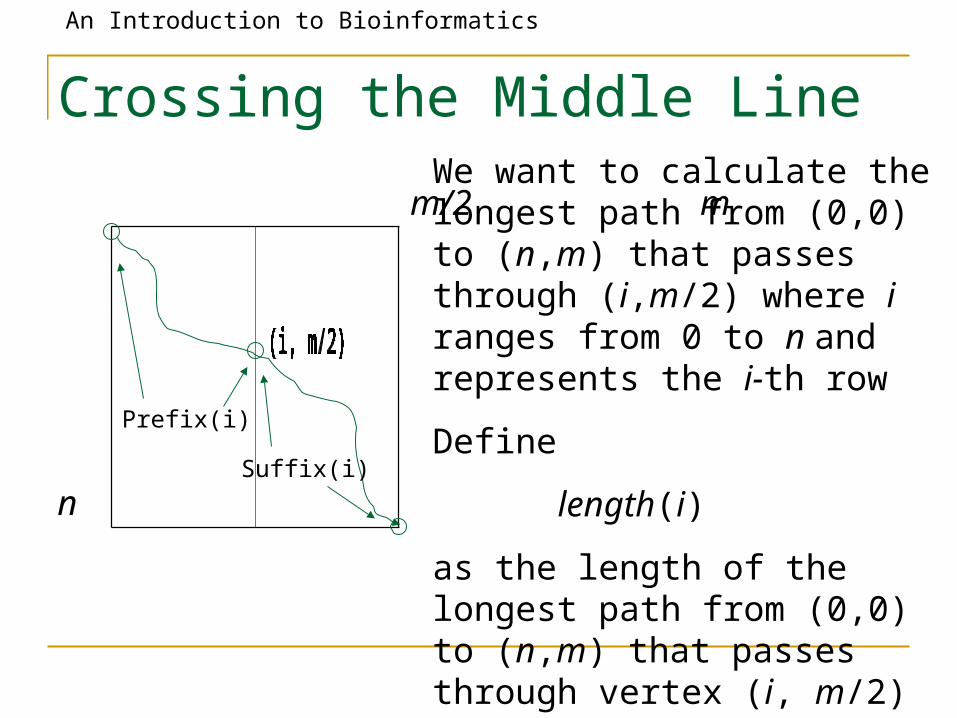
Crossing the Middle Line

m/2 m

n

Prefix(i)

Suffix(i)

We want to calculate the longest path from (0,0) to (n,m) that passes through (i,m/2) where i ranges from 0 to n and represents the i-th row

Define

length(i)

as the length of the longest path from (0,0) to (n,m) that passes through vertex (i, m/2)


m/2 m

n

Prefix(i)

Suffix(i)

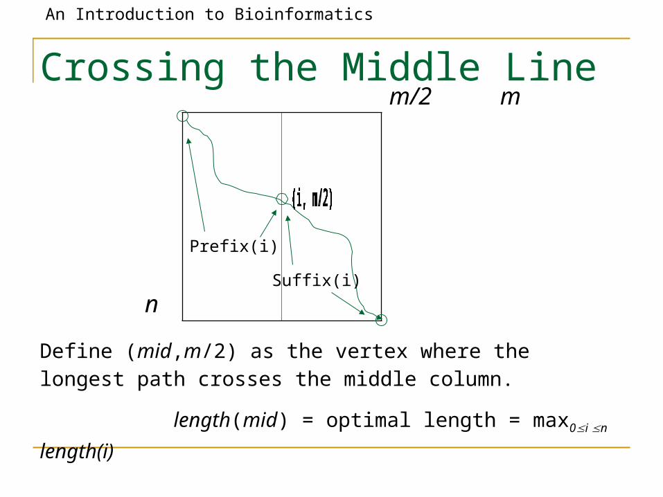
Define (mid,m/2) as the vertex where the longest path crosses the middle column.

length(mid) = optimal length = max0i n length(i)

Crossing the Middle Line


Computing Prefix(i)• prefix(i) is the length of the longest path from

(0,0) to (i,m/2)• Compute prefix(i) by dynamic programming in

the left half of the matrix

0 m/2 m

store prefix(i) column


Computing Suffix(i)• suffix(i) is the length of the longest path from (i,m/2) to (n,m)• suffix(i) is the length of the longest path from (n,m) to (i,m/2)

with all edges reversed• Compute suffix(i) by dynamic programming in the right half

of the “reversed” matrix

0 m/2 m

store suffix(i) column


Length(i) = Prefix(i) + Suffix(i)

• Add prefix(i) and suffix(i) to compute length(i):• length(i)=prefix(i) + suffix(i)

• You now have a middle vertex of the maximum path (i,m/2) as maximum of length(i)

middle point found

0 m/2 m

0

i


Finding the Middle Point0 m/4 m/2 3m/4 m


Finding the Middle Point again0 m/4 m/2 3m/4 m


And Again0 m/8 m/4 3m/8 m/2 5m/8 3m/4 7m/8 m


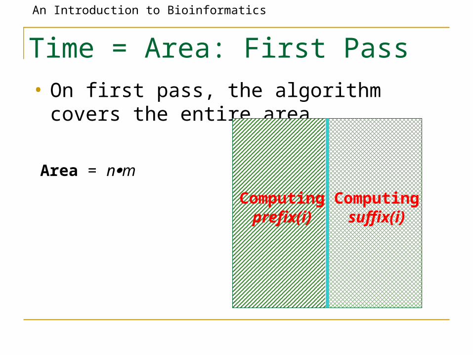
Time = Area: First Pass• On first pass, the algorithm covers the entire

area

Area = nm


Time = Area: First Pass• On first pass, the algorithm covers the entire

area

Area = nm

Computing prefix(i)

Computing suffix(i)


Time = Area: Second Pass• On second pass, the algorithm covers only

1/2 of the area

Area/2


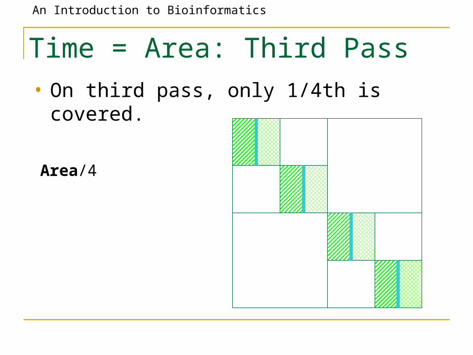
Time = Area: Third Pass• On third pass, only 1/4th is covered.

Area/4


Geometric Reduction At Each Iteration1 + ½ + ¼ + ... + (½)k ≤ 2• Runtime: O(Area) = O(nm)

first pass: 1

2nd pass: 1/2

3rd pass: 1/4

5th pass: 1/16

4th pass: 1/8


Indexing-based Local Aligners

BLAST, WU-BLAST, BlastZ, MegaBLAST, BLAT, PatternHunter, ……


Some useful applications of alignments• Given a newly discovered gene,

• Does it occur in other species?• How fast does it evolve?

• Assume we try Smith-Waterman:

The entire genomic database

Our new gene

104

1010 - 1011


Some useful applications of alignments• Given a newly sequenced organism,• Which subregions align with other organisms?

• Potential genes• Other biological characteristics

• Assume we try Smith-Waterman:

The entire genomic database

Our newly sequenced mammal

3109

1010 - 1011


Indexing-based local alignment

(BLAST- Basic Local Alignment Search Tool)

Main idea:

1. Construct a dictionary of all the words in the query

2. Initiate a local alignment for each word match between query and DB

Running Time: O(MN)

However, orders of magnitude faster than Smith-Waterman

query

DB


Indexing-based local alignmentDictionary:

All words of length k (~10)

Alignment initiated between words of alignment score T

(typically T = k)

Alignment:

Ungapped extensions until score

below statistical threshold

Output:

All local alignments with score

> statistical threshold

……

……

query

DB

query

scan


Indexing-based local alignment—Extensions A C G A A G T A A G G T C C A G T

C

C

C

T

T

C C

T

G

G

A T

T

G

C

G

A

Example:

k = 4

The matching word GGTC initiates an alignment

Extension to the left and right with no gaps until alignment falls < T below best so far

Output:

GTAAGGTCC

GTTAGGTCC



C

T

G

A

T

C C

T

G

G

A

T

T

G C

G

A

Gapped extensions

• Extensions with gaps in a band around anchor

Output:

GTAAGGTCCAGTGTTAGGTC-AGT



C

T

G

A

T

C C

T

G

G

A

T

T

G C

G

A

Gapped extensions until threshold

• Extensions with gaps until score < T below best score so far

Output:

GTAAGGTCCAGTGTTAGGTC-AGT


Indexing-based local alignment—The index• Sensitivity/speed

tradeoff

long words

(k = 15)

short words

(k = 7)

Sensitivity

Speed

Kent WJ, Genome Research 2002

Sens.

Speed


Indexing-based local alignment—The indexMethods to improve sensitivity/speed

1. Using pairs of words

2. Using inexact words

3. Patterns—non consecutive positions

……ATAACGGACGACTGATTACACTGATTCTTAC……

……GGCACGGACCAGTGACTACTCTGATTCCCAG……

……ATAACGGACGACTGATTACACTGATTCTTAC……

……GGCGCCGACGAGTGATTACACAGATTGCCAG……

TTTGATTACACAGAT T G TT CAC G


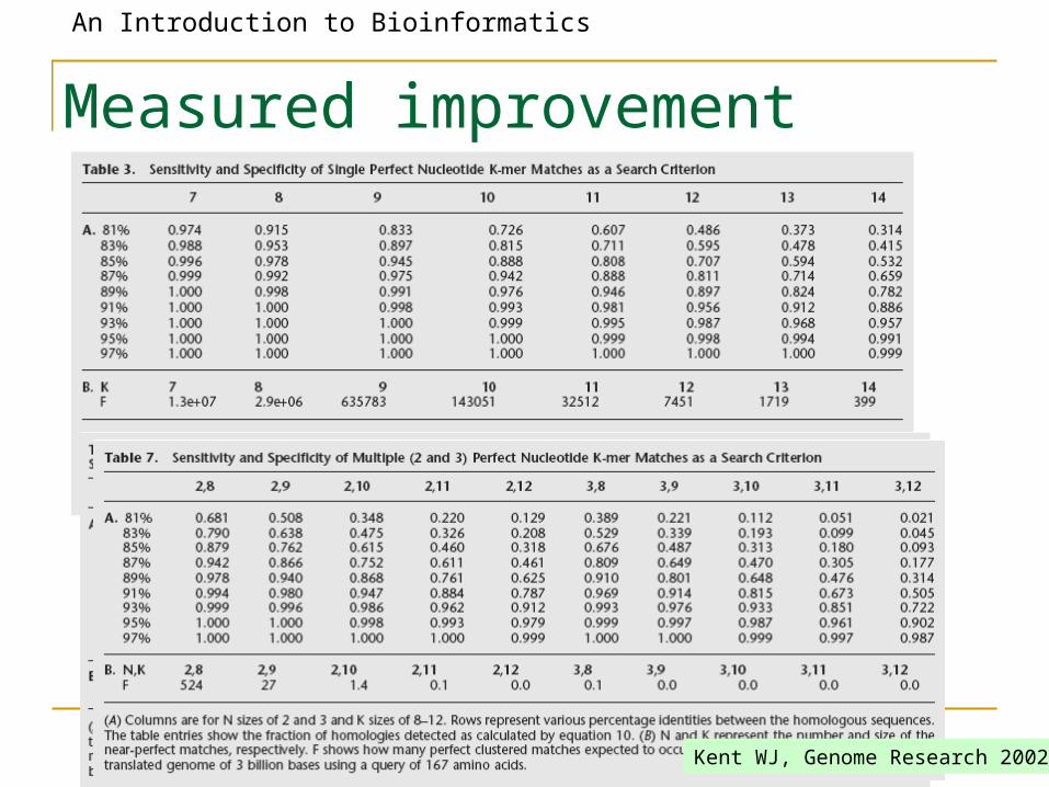
Measured improvement

Kent WJ, Genome Research 2002


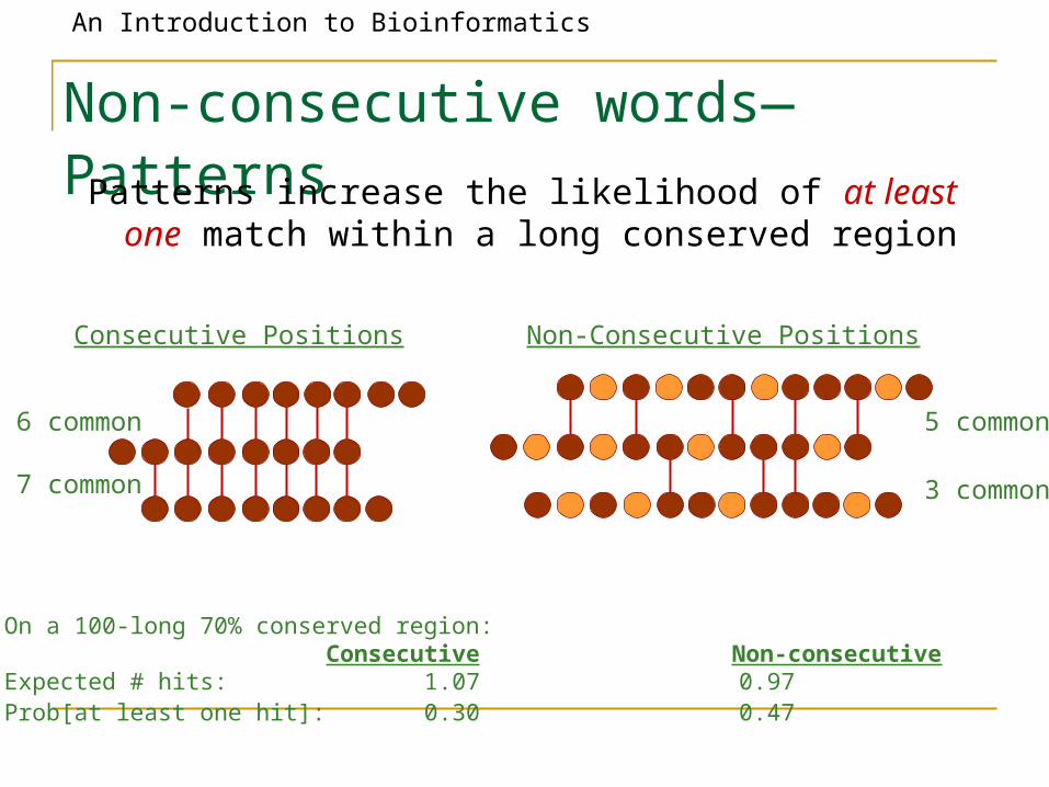
Non-consecutive words—Patterns Patterns increase the likelihood of at least one

match within a long conserved region

3 common

5 common

7 common

Consecutive Positions Non-Consecutive Positions

6 common

On a 100-long 70% conserved region: Consecutive Non-consecutive

Expected # hits: 1.07 0.97Prob[at least one hit]: 0.30 0.47


Advantage of Patterns

11 positions

11 positions

10 positions


Multiple patterns

• K patterns• Takes K times longer to scan• Patterns can complement one another

• Computational problem:• Given: a model (prob distribution) for homology between two regions• Find: best set of K patterns that maximizes Prob(at least one match)

TTTGATTACACAGAT T G TT CAC G T G T C CAG TTGATT A G

Buhler et al. RECOMB 2003Sun & Buhler RECOMB 2004

How long does it take to search the query?


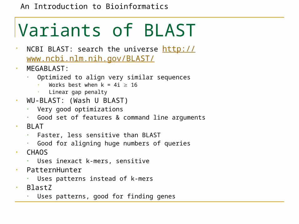
Variants of BLAST• NCBI BLAST: search the universe http://www.ncbi.nlm.nih.gov/BLAST/• MEGABLAST:

• Optimized to align very similar sequences• Works best when k = 4i 16• Linear gap penalty

• WU-BLAST: (Wash U BLAST)• Very good optimizations• Good set of features & command line arguments

• BLAT• Faster, less sensitive than BLAST• Good for aligning huge numbers of queries

• CHAOS• Uses inexact k-mers, sensitive

• PatternHunter• Uses patterns instead of k-mers

• BlastZ• Uses patterns, good for finding genes


ExampleQuery: gattacaccccgattacaccccgattaca (29 letters) [2 mins]

Database: All GenBank+EMBL+DDBJ+PDB sequences (but no EST, STS, GSS, or phase 0, 1 or 2 HTGS sequences) 1,726,556 sequences; 8,074,398,388 total letters

>gi|28570323|gb|AC108906.9| Oryza sativa chromosome 3 BAC OSJNBa0087C10 genomic sequence, complete sequence Length = 144487 Score = 34.2 bits (17), Expect = 4.5 Identities = 20/21 (95%) Strand = Plus / Plus

Query: 4 tacaccccgattacaccccga 24 ||||||| |||||||||||||

Sbjct: 125138 tacacccagattacaccccga 125158

Score = 34.2 bits (17),

Expect = 4.5 Identities = 20/21 (95%) Strand = Plus / Plus



>gi|28173089|gb|AC104321.7| Oryza sativa chromosome 3 BAC OSJNBa0052F07 genomic sequence, complete sequence Length = 139823 Score = 34.2 bits (17), Expect = 4.5 Identities = 20/21 (95%) Strand = Plus / Plus




ExampleQuery: Human atoh enhancer, 179 letters [1.5 min]

Result: 57 blast hits1. gi|7677270|gb|AF218259.1|AF218259 Homo sapiens ATOH1 enhanc... 355 1e-95 2. gi|22779500|gb|AC091158.11| Mus musculus Strain C57BL6/J ch... 264 4e-68 3. gi|7677269|gb|AF218258.1|AF218258 Mus musculus Atoh1 enhanc... 256 9e-66 4. gi|28875397|gb|AF467292.1| Gallus gallus CATH1 (CATH1) gene... 78 5e-12 5. gi|27550980|emb|AL807792.6| Zebrafish DNA sequence from clo... 54 7e-05 6. gi|22002129|gb|AC092389.4| Oryza sativa chromosome 10 BAC O... 44 0.068 7. gi|22094122|ref|NM_013676.1| Mus musculus suppressor of Ty ... 42 0.27 8. gi|13938031|gb|BC007132.1| Mus musculus, Similar to suppres... 42 0.27

gi|7677269|gb|AF218258.1|AF218258 Mus musculus Atoh1 enhancer sequence Length = 1517 Score = 256 bits (129), Expect = 9e-66 Identities = 167/177 (94%),

Gaps = 2/177 (1%) Strand = Plus / Plus Query: 3 tgacaatagagggtctggcagaggctcctggccgcggtgcggagcgtctggagcggagca 62 ||||||||||||| ||||||||||||||||||| |||||||||||||||||||||||||| Sbjct: 1144 tgacaatagaggggctggcagaggctcctggccccggtgcggagcgtctggagcggagca 1203

Query: 63 cgcgctgtcagctggtgagcgcactctcctttcaggcagctccccggggagctgtgcggc 122 |||||||||||||||||||||||||| ||||||||| |||||||||||||||| ||||| Sbjct: 1204 cgcgctgtcagctggtgagcgcactc-gctttcaggccgctccccggggagctgagcggc 1262

Query: 123 cacatttaacaccatcatcacccctccccggcctcctcaacctcggcctcctcctcg 179 ||||||||||||| || ||| |||||||||||||||||||| |||||||||||||||

Sbjct: 1263 cacatttaacaccgtcgtca-ccctccccggcctcctcaacatcggcctcctcctcg 1318

an introduction to bioinformatics 2. comparing biological sequences: sequence alignment (cont’d)

Documents

j s i

w j slide

w j s i

bioinformatics scoring

bioinformatics simple

mismatch s i

penalty slide

indels slide