1 (c) mark gerstein, 1999, yale, bioinfo.mbb.yale.edu bioinformatics sequences mark gerstein, yale...
Post on 20-Dec-2015
217 views
TRANSCRIPT
1
(c)
Mar
k G
erst
ein
, 19
99,
Yal
e, b
ioin
fo.m
bb
.yal
e.ed
u
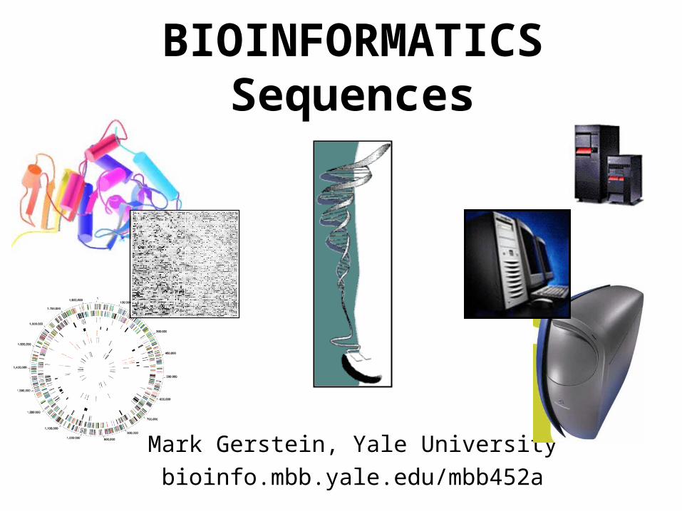
BIOINFORMATICSSequences
Mark Gerstein, Yale University
bioinfo.mbb.yale.edu/mbb452a
2
(c)
Mar
k G
erst
ein
, 19
99,
Yal
e, b
ioin
fo.m
bb
.yal
e.ed
u
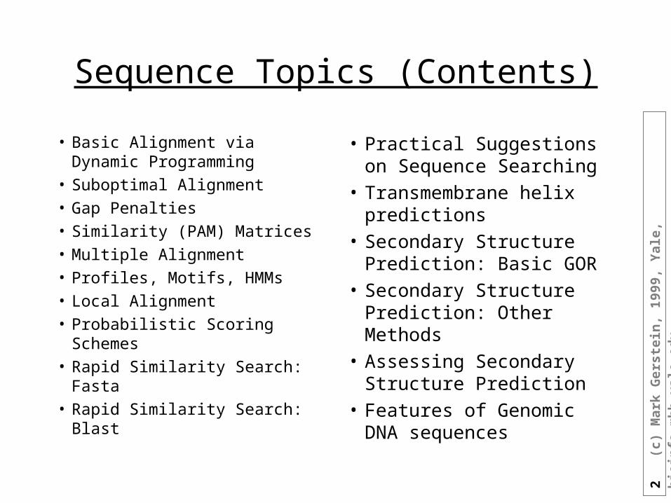
Sequence Topics (Contents)
• Basic Alignment via Dynamic Programming
• Suboptimal Alignment• Gap Penalties• Similarity (PAM) Matrices• Multiple Alignment• Profiles, Motifs, HMMs• Local Alignment• Probabilistic Scoring Schemes• Rapid Similarity Search: Fasta• Rapid Similarity Search: Blast
• Practical Suggestions on Sequence Searching
• Transmembrane helix predictions
• Secondary Structure Prediction: Basic GOR
• Secondary Structure Prediction: Other Methods
• Assessing Secondary Structure Prediction
• Features of Genomic DNA sequences
3
(c)
Mar
k G
erst
ein
, 19
99,
Yal
e, b
ioin
fo.m
bb
.yal
e.ed
u
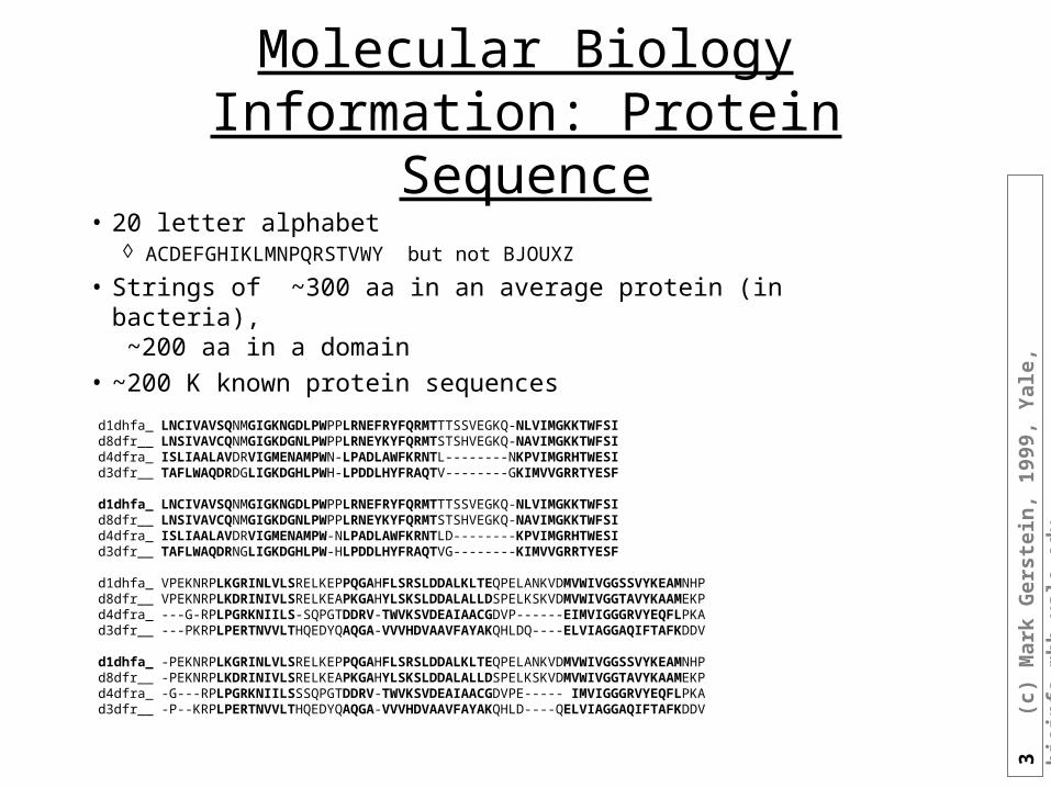
Molecular Biology Information: Protein Sequence
• 20 letter alphabet ACDEFGHIKLMNPQRSTVWY but not BJOUXZ
• Strings of ~300 aa in an average protein (in bacteria), ~200 aa in a domain
• ~200 K known protein sequencesd1dhfa_ LNCIVAVSQNMGIGKNGDLPWPPLRNEFRYFQRMTTTSSVEGKQ-NLVIMGKKTWFSI d8dfr__ LNSIVAVCQNMGIGKDGNLPWPPLRNEYKYFQRMTSTSHVEGKQ-NAVIMGKKTWFSI d4dfra_ ISLIAALAVDRVIGMENAMPWN-LPADLAWFKRNTL--------NKPVIMGRHTWESI d3dfr__ TAFLWAQDRDGLIGKDGHLPWH-LPDDLHYFRAQTV--------GKIMVVGRRTYESF d1dhfa_ LNCIVAVSQNMGIGKNGDLPWPPLRNEFRYFQRMTTTSSVEGKQ-NLVIMGKKTWFSId8dfr__ LNSIVAVCQNMGIGKDGNLPWPPLRNEYKYFQRMTSTSHVEGKQ-NAVIMGKKTWFSId4dfra_ ISLIAALAVDRVIGMENAMPW-NLPADLAWFKRNTLD--------KPVIMGRHTWESId3dfr__ TAFLWAQDRNGLIGKDGHLPW-HLPDDLHYFRAQTVG--------KIMVVGRRTYESF
d1dhfa_ VPEKNRPLKGRINLVLSRELKEPPQGAHFLSRSLDDALKLTEQPELANKVDMVWIVGGSSVYKEAMNHPd8dfr__ VPEKNRPLKDRINIVLSRELKEAPKGAHYLSKSLDDALALLDSPELKSKVDMVWIVGGTAVYKAAMEKPd4dfra_ ---G-RPLPGRKNIILS-SQPGTDDRV-TWVKSVDEAIAACGDVP------EIMVIGGGRVYEQFLPKAd3dfr__ ---PKRPLPERTNVVLTHQEDYQAQGA-VVVHDVAAVFAYAKQHLDQ----ELVIAGGAQIFTAFKDDV d1dhfa_ -PEKNRPLKGRINLVLSRELKEPPQGAHFLSRSLDDALKLTEQPELANKVDMVWIVGGSSVYKEAMNHPd8dfr__ -PEKNRPLKDRINIVLSRELKEAPKGAHYLSKSLDDALALLDSPELKSKVDMVWIVGGTAVYKAAMEKPd4dfra_ -G---RPLPGRKNIILSSSQPGTDDRV-TWVKSVDEAIAACGDVPE-----.IMVIGGGRVYEQFLPKAd3dfr__ -P--KRPLPERTNVVLTHQEDYQAQGA-VVVHDVAAVFAYAKQHLD----QELVIAGGAQIFTAFKDDV
4
(c)
Mar
k G
erst
ein
, 19
99,
Yal
e, b
ioin
fo.m
bb
.yal
e.ed
u
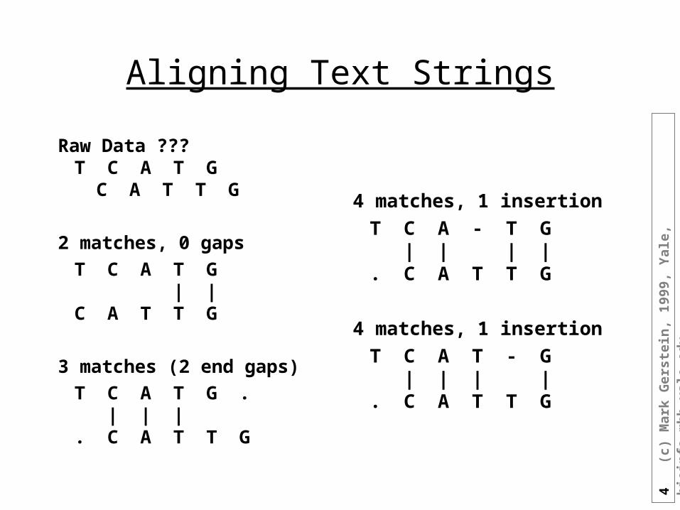
Aligning Text Strings
Raw Data ???T C A T G C A T T G
2 matches, 0 gaps
T C A T G | |C A T T G
3 matches (2 end gaps)
T C A T G . | | | . C A T T G
4 matches, 1 insertion
T C A - T G | | | | . C A T T G
4 matches, 1 insertion
T C A T - G | | | | . C A T T G
5
(c)
Mar
k G
erst
ein
, 19
99,
Yal
e, b
ioin
fo.m
bb
.yal
e.ed
u
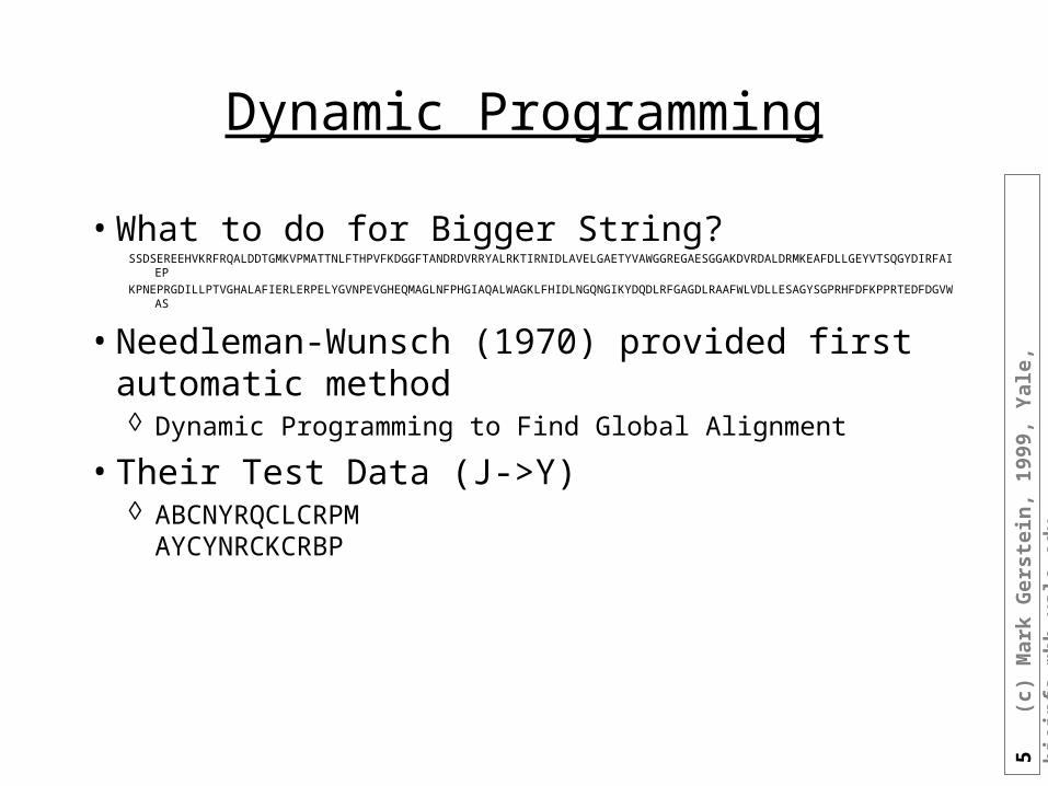
Dynamic Programming
• What to do for Bigger String?SSDSEREEHVKRFRQALDDTGMKVPMATTNLFTHPVFKDGGFTANDRDVRRYALRKTIRNIDLAVELGAETYVAWGGREGAESGGAKDVRDALDRMKEAFDLLGEYVTSQGYDIRFAI
EP
KPNEPRGDILLPTVGHALAFIERLERPELYGVNPEVGHEQMAGLNFPHGIAQALWAGKLFHIDLNGQNGIKYDQDLRFGAGDLRAAFWLVDLLESAGYSGPRHFDFKPPRTEDFDGVWAS
• Needleman-Wunsch (1970) provided first automatic method Dynamic Programming to Find Global Alignment
• Their Test Data (J->Y) ABCNYRQCLCRPMAYCYNRCKCRBP
6
(c)
Mar
k G
erst
ein
, 19
99,
Yal
e, b
ioin
fo.m
bb
.yal
e.ed
u
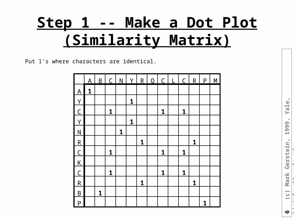
Step 1 -- Make a Dot Plot (Similarity Matrix)
Put 1's where characters are identical.
A B C N Y R Q C L C R P M
A 1
Y 1
C 1 1 1
Y 1
N 1
R 1 1
C 1 1 1
K
C 1 1 1
R 1 1
B 1
P 1
7
(c)
Mar
k G
erst
ein
, 19
99,
Yal
e, b
ioin
fo.m
bb
.yal
e.ed
u
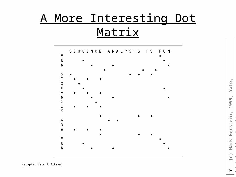
A More Interesting Dot Matrix
(adapted from R Altman)
8
(c)
Mar
k G
erst
ein
, 19
99,
Yal
e, b
ioin
fo.m
bb
.yal
e.ed
u
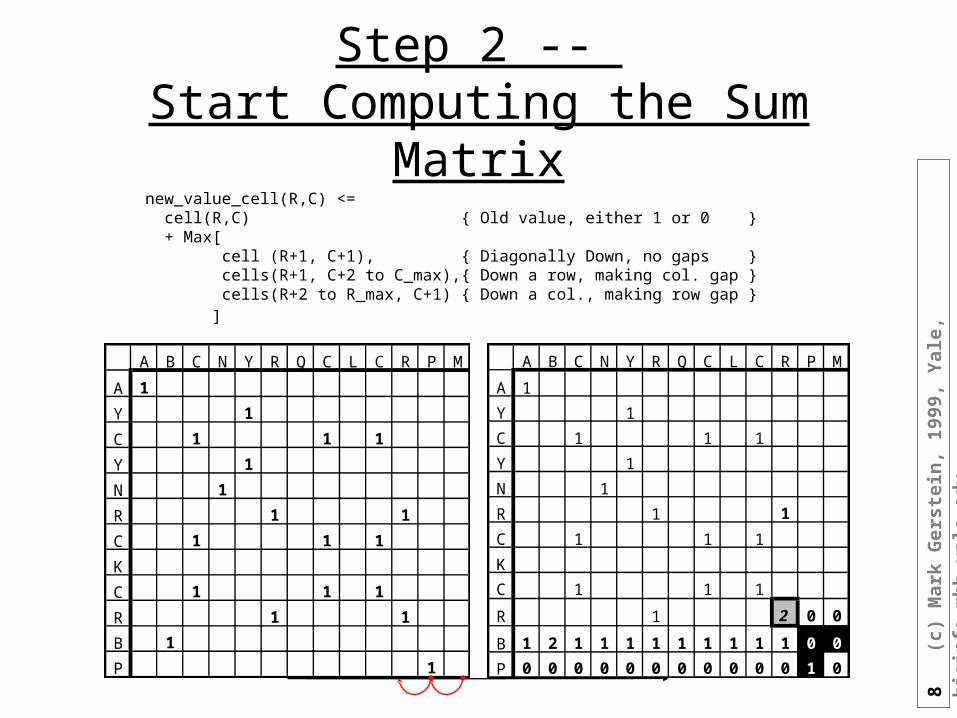
Step 2 -- Start Computing the Sum Matrixnew_value_cell(R,C) <= cell(R,C) { Old value, either 1 or 0 } + Max[ cell (R+1, C+1), { Diagonally Down, no gaps } cells(R+1, C+2 to C_max),{ Down a row, making col. gap } cells(R+2 to R_max, C+1) { Down a col., making row gap } ]
A B C N Y R Q C L C R P M
A 1
Y 1
C 1 1 1
Y 1
N 1
R 1 1
C 1 1 1
K
C 1 1 1
R 1 2 0 0
B 1 2 1 1 1 1 1 1 1 1 1 0 0
P 0 0 0 0 0 0 0 0 0 0 0 1 0
A B C N Y R Q C L C R P M
A 1
Y 1
C 1 1 1
Y 1
N 1
R 1 1
C 1 1 1
K
C 1 1 1
R 1 1
B 1
P 1
9
(c)
Mar
k G
erst
ein
, 19
99,
Yal
e, b
ioin
fo.m
bb
.yal
e.ed
u
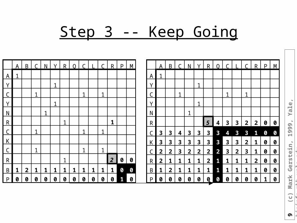
Step 3 -- Keep Going
A B C N Y R Q C L C R P M
A 1
Y 1
C 1 1 1
Y 1
N 1
R 5 4 3 3 2 2 0 0
C 3 3 4 3 3 3 3 4 3 3 1 0 0
K 3 3 3 3 3 3 3 3 3 2 1 0 0
C 2 2 3 2 2 2 2 3 2 3 1 0 0
R 2 1 1 1 1 2 1 1 1 1 2 0 0
B 1 2 1 1 1 1 1 1 1 1 1 0 0
P 0 0 0 0 0 0 0 0 0 0 0 1 0
A B C N Y R Q C L C R P M
A 1
Y 1
C 1 1 1
Y 1
N 1
R 1 1
C 1 1 1
K
C 1 1 1
R 1 2 0 0
B 1 2 1 1 1 1 1 1 1 1 1 0 0
P 0 0 0 0 0 0 0 0 0 0 0 1 0
10
(c)
Mar
k G
erst
ein
, 19
99,
Yal
e, b
ioin
fo.m
bb
.yal
e.ed
u
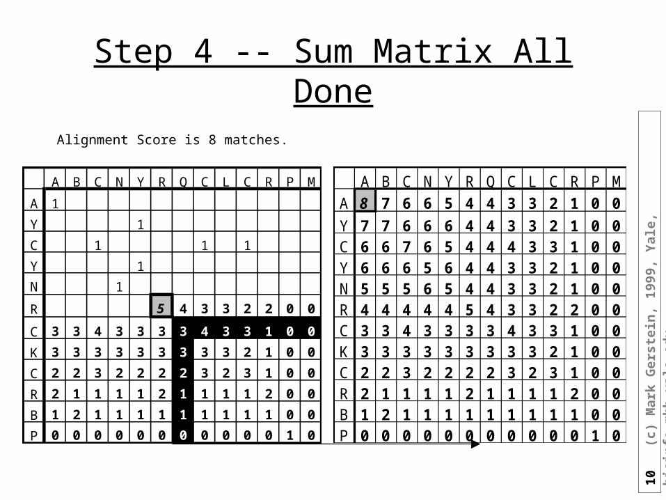
Step 4 -- Sum Matrix All Done
Alignment Score is 8 matches.
A B C N Y R Q C L C R P MA 8 7 6 6 5 4 4 3 3 2 1 0 0
Y 7 7 6 6 6 4 4 3 3 2 1 0 0C 6 6 7 6 5 4 4 4 3 3 1 0 0Y 6 6 6 5 6 4 4 3 3 2 1 0 0N 5 5 5 6 5 4 4 3 3 2 1 0 0R 4 4 4 4 4 5 4 3 3 2 2 0 0C 3 3 4 3 3 3 3 4 3 3 1 0 0K 3 3 3 3 3 3 3 3 3 2 1 0 0C 2 2 3 2 2 2 2 3 2 3 1 0 0R 2 1 1 1 1 2 1 1 1 1 2 0 0B 1 2 1 1 1 1 1 1 1 1 1 0 0P 0 0 0 0 0 0 0 0 0 0 0 1 0
A B C N Y R Q C L C R P M
A 1
Y 1
C 1 1 1
Y 1
N 1
R 5 4 3 3 2 2 0 0
C 3 3 4 3 3 3 3 4 3 3 1 0 0
K 3 3 3 3 3 3 3 3 3 2 1 0 0
C 2 2 3 2 2 2 2 3 2 3 1 0 0
R 2 1 1 1 1 2 1 1 1 1 2 0 0
B 1 2 1 1 1 1 1 1 1 1 1 0 0
P 0 0 0 0 0 0 0 0 0 0 0 1 0
11
(c)
Mar
k G
erst
ein
, 19
99,
Yal
e, b
ioin
fo.m
bb
.yal
e.ed
u
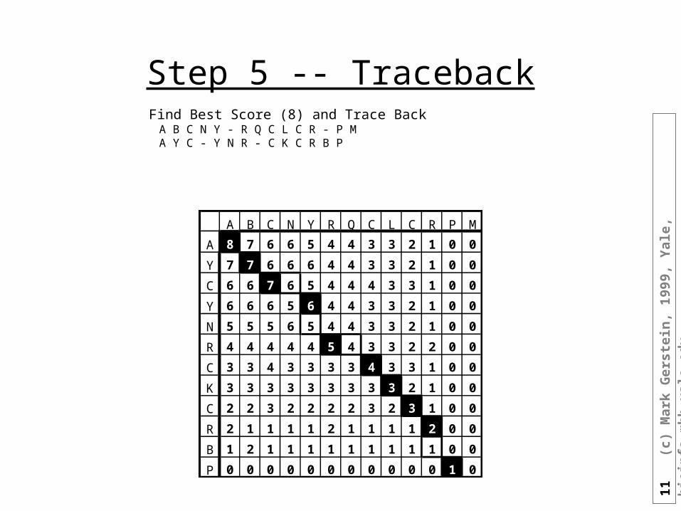
Step 5 -- TracebackFind Best Score (8) and Trace BackA B C N Y - R Q C L C R - P MA Y C - Y N R - C K C R B P
A B C N Y R Q C L C R P M
A 8 7 6 6 5 4 4 3 3 2 1 0 0
Y 7 7 6 6 6 4 4 3 3 2 1 0 0
C 6 6 7 6 5 4 4 4 3 3 1 0 0
Y 6 6 6 5 6 4 4 3 3 2 1 0 0
N 5 5 5 6 5 4 4 3 3 2 1 0 0
R 4 4 4 4 4 5 4 3 3 2 2 0 0
C 3 3 4 3 3 3 3 4 3 3 1 0 0
K 3 3 3 3 3 3 3 3 3 2 1 0 0
C 2 2 3 2 2 2 2 3 2 3 1 0 0
R 2 1 1 1 1 2 1 1 1 1 2 0 0
B 1 2 1 1 1 1 1 1 1 1 1 0 0
P 0 0 0 0 0 0 0 0 0 0 0 1 0
12
(c)
Mar
k G
erst
ein
, 19
99,
Yal
e, b
ioin
fo.m
bb
.yal
e.ed
u
Step 5 -- TracebackA B C N Y - R Q C L C R - P MA Y C - Y N R - C K C R B P
A B C N Y R Q C L C R P M
A 8 7 6 6 5 4 4 3 3 2 1 0 0
Y 7 7 6 6 6 4 4 3 3 2 1 0 0
C 6 6 7 6 5 4 4 4 3 3 1 0 0
Y 6 6 6 5 6 4 4 3 3 2 1 0 0
N 5 5 5 6 5 4 4 3 3 2 1 0 0
R 4 4 4 4 4 5 4 3 3 2 2 0 0
C 3 3 4 3 3 3 3 4 3 3 1 0 0
K 3 3 3 3 3 3 3 3 3 2 1 0 0
C 2 2 3 2 2 2 2 3 2 3 1 0 0
R 2 1 1 1 1 2 1 1 1 1 2 0 0
B 1 2 1 1 1 1 1 1 1 1 1 0 0
P 0 0 0 0 0 0 0 0 0 0 0 1 0
13
(c)
Mar
k G
erst
ein
, 19
99,
Yal
e, b
ioin
fo.m
bb
.yal
e.ed
u
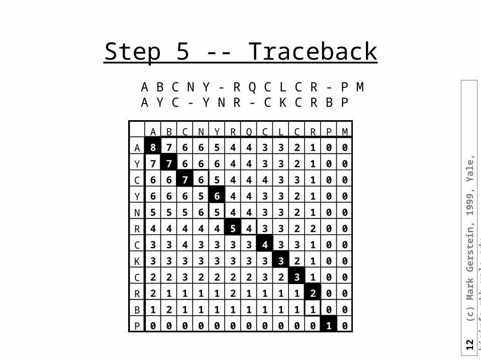
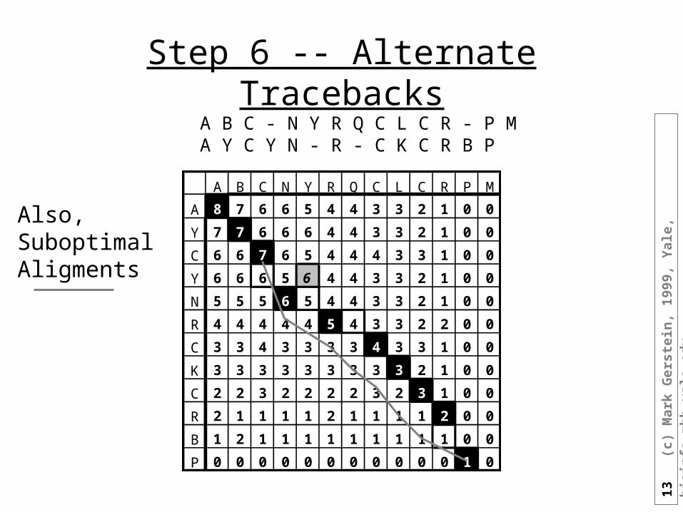
Step 6 -- Alternate TracebacksA B C - N Y R Q C L C R - P MA Y C Y N - R - C K C R B P
A B C N Y R Q C L C R P M
A 8 7 6 6 5 4 4 3 3 2 1 0 0
Y 7 7 6 6 6 4 4 3 3 2 1 0 0
C 6 6 7 6 5 4 4 4 3 3 1 0 0
Y 6 6 6 5 6 4 4 3 3 2 1 0 0
N 5 5 5 6 5 4 4 3 3 2 1 0 0
R 4 4 4 4 4 5 4 3 3 2 2 0 0
C 3 3 4 3 3 3 3 4 3 3 1 0 0
K 3 3 3 3 3 3 3 3 3 2 1 0 0
C 2 2 3 2 2 2 2 3 2 3 1 0 0
R 2 1 1 1 1 2 1 1 1 1 2 0 0
B 1 2 1 1 1 1 1 1 1 1 1 0 0
P 0 0 0 0 0 0 0 0 0 0 0 1 0
Also, SuboptimalAligments
14
(c)
Mar
k G
erst
ein
, 19
99,
Yal
e, b
ioin
fo.m
bb
.yal
e.ed
u
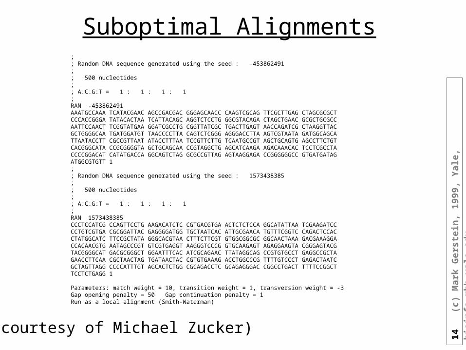
Suboptimal Alignments
(courtesy of Michael Zucker)
; ; Random DNA sequence generated using the seed : -453862491 ; ; 500 nucleotides ; ; A:C:G:T = 1 : 1 : 1 : 1 ; RAN -453862491 AAATGCCAAA TCATACGAAC AGCCGACGAC GGGAGCAACC CAAGTCGCAG TTCGCTTGAG CTAGCGCGCT CCCACCGGGA TATACACTAA TCATTACAGC AGGTCTCCTG GGCGTACAGA CTAGCTGAAC GCGCTGCGCC AATTCCAACT TCGGTATGAA GGATCGCCTG CGGTTATCGC TGACTTGAGT AACCAGATCG CTAAGGTTAC GCTGGGGCAA TGATGGATGT TAACCCCTTA CAGTCTCGGG AGGGACCTTA AGTCGTAATA GATGGCAGCA TTAATACCTT CGCCGTTAAT ATACCTTTAA TCCGTTCTTG TCAATGCCGT AGCTGCAGTG AGCCTTCTGT CACGGGCATA CCGCGGGGTA GCTGCAGCAA CCGTAGGCTG AGCATCAAGA AGACAAACAC TCCTCGCCTA CCCCGGACAT CATATGACCA GGCAGTCTAG GCGCCGTTAG AGTAAGGAGA CCGGGGGGCC GTGATGATAG ATGGCGTGTT 1 ; ; Random DNA sequence generated using the seed : 1573438385 ; ; 500 nucleotides ; ; A:C:G:T = 1 : 1 : 1 : 1 ; RAN 1573438385 CCCTCCATCG CCAGTTCCTG AAGACATCTC CGTGACGTGA ACTCTCTCCA GGCATATTAA TCGAAGATCC CCTGTCGTGA CGCGGATTAC GAGGGGATGG TGCTAATCAC ATTGCGAACA TGTTTCGGTC CAGACTCCAC CTATGGCATC TTCCGCTATA GGGCACGTAA CTTTCTTCGT GTGGCGGCGC GGCAACTAAA GACGAAAGGA CCACAACGTG AATAGCCCGT GTCGTGAGGT AAGGGTCCCG GTGCAAGAGT AGAGGAAGTA CGGGAGTACG TACGGGGCAT GACGCGGGCT GGAATTTCAC ATCGCAGAAC TTATAGGCAG CCGTGTGCCT GAGGCCGCTA GAACCTTCAA CGCTAACTAG TGATAACTAC CGTGTGAAAG ACCTGGCCCG TTTTGTCCCT GAGACTAATC GCTAGTTAGG CCCCATTTGT AGCACTCTGG CGCAGACCTC GCAGAGGGAC CGGCCTGACT TTTTCCGGCT TCCTCTGAGG 1
Parameters: match weight = 10, transition weight = 1, transversion weight = -3 Gap opening penalty = 50 Gap continuation penalty = 1 Run as a local alignment (Smith-Waterman)
15
(c)
Mar
k G
erst
ein
, 19
99,
Yal
e, b
ioin
fo.m
bb
.yal
e.ed
u
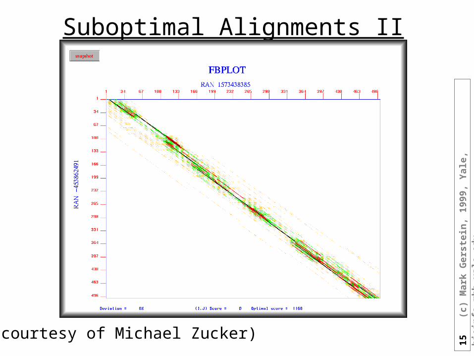
Suboptimal Alignments II
(courtesy of Michael Zucker)
16
(c)
Mar
k G
erst
ein
, 19
99,
Yal
e, b
ioin
fo.m
bb
.yal
e.ed
u
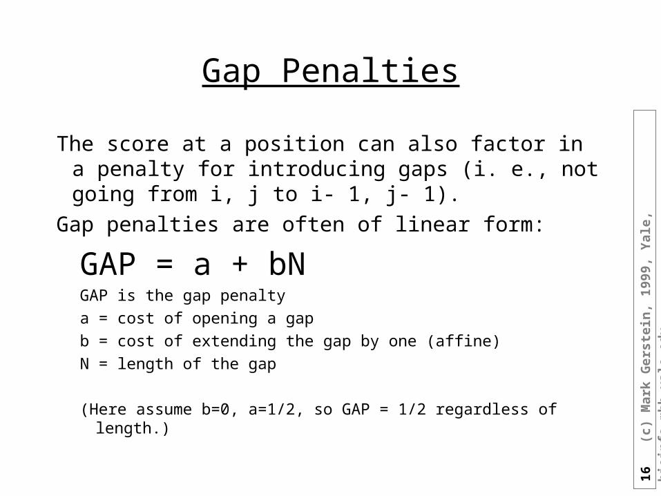
Gap Penalties
The score at a position can also factor in a penalty for introducing gaps (i. e., not going from i, j to i- 1, j- 1).
Gap penalties are often of linear form:
GAP = a + bNGAP is the gap penalty
a = cost of opening a gap
b = cost of extending the gap by one (affine)
N = length of the gap
(Here assume b=0, a=1/2, so GAP = 1/2 regardless of length.)
17
(c)
Mar
k G
erst
ein
, 19
99,
Yal
e, b
ioin
fo.m
bb
.yal
e.ed
u
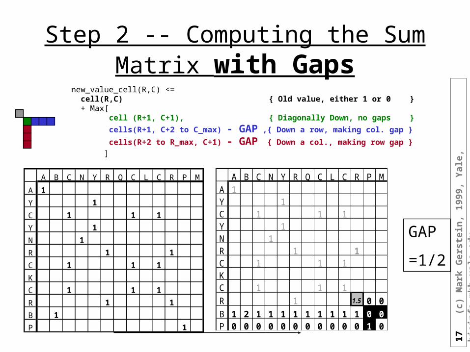
Step 2 -- Computing the Sum Matrix with Gaps
new_value_cell(R,C) <= cell(R,C) { Old value, either 1 or 0 } + Max[ cell (R+1, C+1), { Diagonally Down, no gaps }
cells(R+1, C+2 to C_max) - GAP ,{ Down a row, making col. gap } cells(R+2 to R_max, C+1) - GAP { Down a col., making row gap } ]
A B C N Y R Q C L C R P M
A 1
Y 1
C 1 1 1
Y 1
N 1
R 1 1
C 1 1 1
K
C 1 1 1
R 1 1
B 1
P 1
A B C N Y R Q C L C R P MA 1Y 1C 1 1 1Y 1N 1R 1 1C 1 1 1KC 1 1 1
R 1 1.5 0 0
B 1 2 1 1 1 1 1 1 1 1 1 0 0P 0 0 0 0 0 0 0 0 0 0 0 1 0
GAP
=1/2
18
(c)
Mar
k G
erst
ein
, 19
99,
Yal
e, b
ioin
fo.m
bb
.yal
e.ed
u
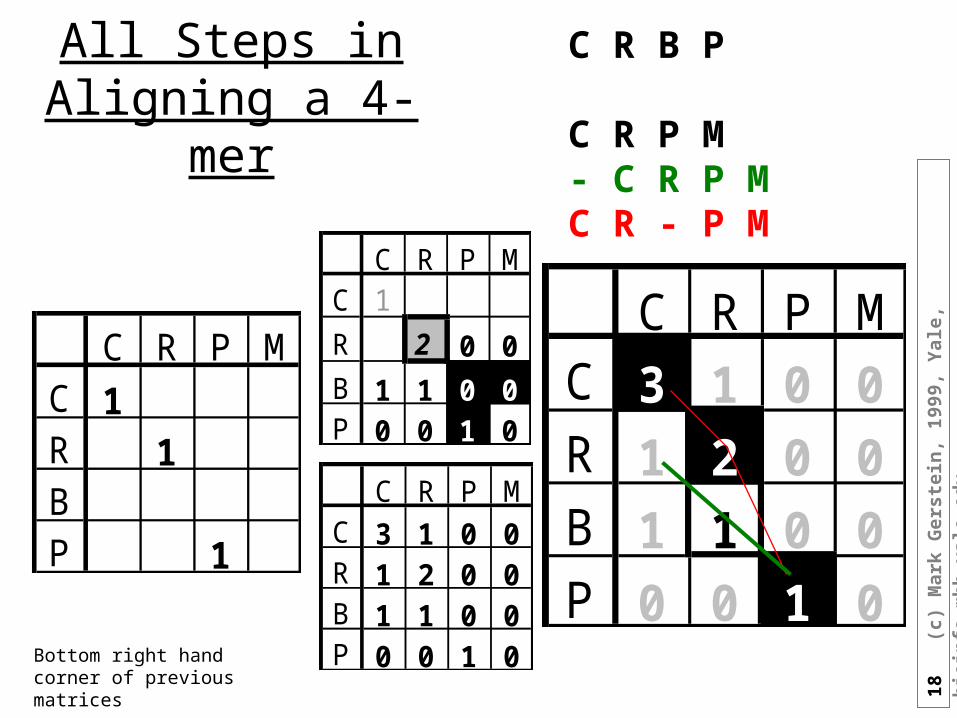
All Steps in Aligning a 4-mer
C R P MC 1R 1BP 1
C R P MC 1
R 2 0 0
B 1 1 0 0P 0 0 1 0
C R P MC 3 1 0 0R 1 2 0 0B 1 1 0 0P 0 0 1 0
C R P MC 3 1 0 0R 1 2 0 0B 1 1 0 0P 0 0 1 0
C R B P
C R P M- C R P MC R - P M
Bottom right hand corner of previous matrices
19
(c)
Mar
k G
erst
ein
, 19
99,
Yal
e, b
ioin
fo.m
bb
.yal
e.ed
u
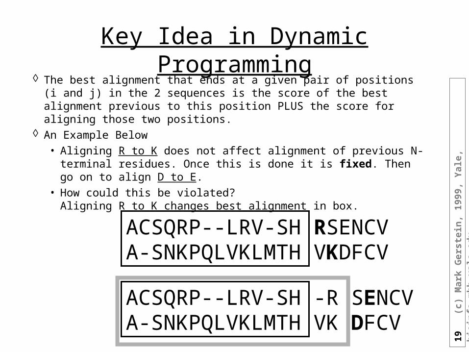
Key Idea in Dynamic Programming The best alignment that ends at a given pair of positions (i and j) in the 2
sequences is the score of the best alignment previous to this position PLUS the score for aligning those two positions.
An Example Below
• Aligning R to K does not affect alignment of previous N-terminal residues. Once this is done it is fixed. Then go on to align D to E.
• How could this be violated? Aligning R to K changes best alignment in box.
ACSQRP--LRV-SH RSENCVA-SNKPQLVKLMTH VKDFCV
ACSQRP--LRV-SH -R SENCVA-SNKPQLVKLMTH VK DFCV
20
(c)
Mar
k G
erst
ein
, 19
99,
Yal
e, b
ioin
fo.m
bb
.yal
e.ed
u
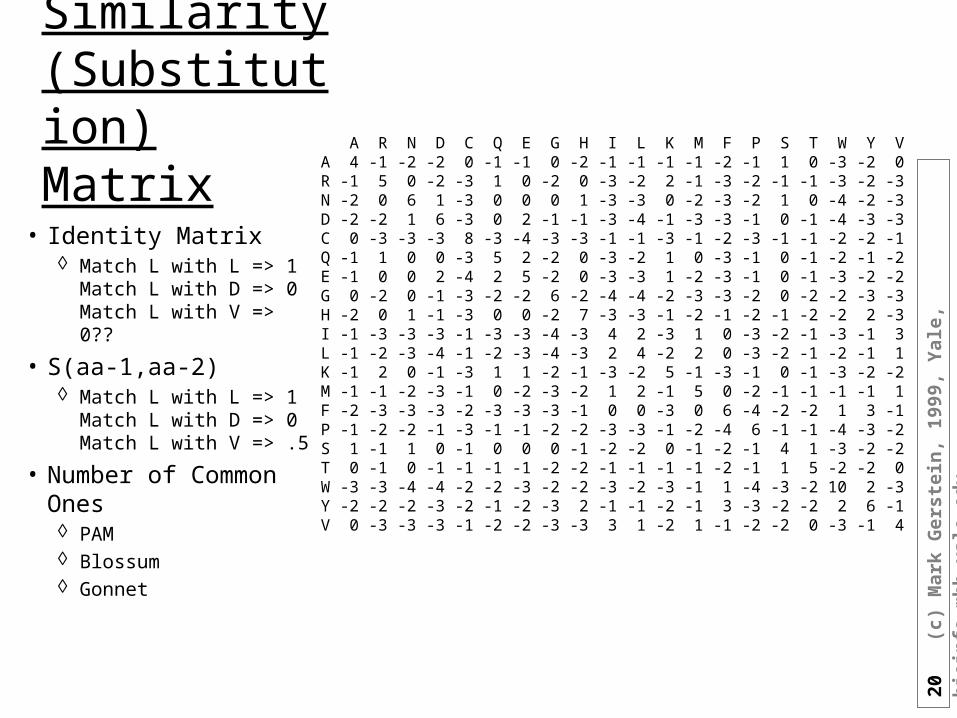
Similarity (Substitution) Matrix
• Identity Matrix Match L with L => 1
Match L with D => 0Match L with V => 0??
• S(aa-1,aa-2) Match L with L => 1
Match L with D => 0Match L with V => .5
• Number of Common Ones PAM Blossum Gonnet
A R N D C Q E G H I L K M F P S T W Y V A 4 -1 -2 -2 0 -1 -1 0 -2 -1 -1 -1 -1 -2 -1 1 0 -3 -2 0 R -1 5 0 -2 -3 1 0 -2 0 -3 -2 2 -1 -3 -2 -1 -1 -3 -2 -3 N -2 0 6 1 -3 0 0 0 1 -3 -3 0 -2 -3 -2 1 0 -4 -2 -3 D -2 -2 1 6 -3 0 2 -1 -1 -3 -4 -1 -3 -3 -1 0 -1 -4 -3 -3 C 0 -3 -3 -3 8 -3 -4 -3 -3 -1 -1 -3 -1 -2 -3 -1 -1 -2 -2 -1 Q -1 1 0 0 -3 5 2 -2 0 -3 -2 1 0 -3 -1 0 -1 -2 -1 -2 E -1 0 0 2 -4 2 5 -2 0 -3 -3 1 -2 -3 -1 0 -1 -3 -2 -2 G 0 -2 0 -1 -3 -2 -2 6 -2 -4 -4 -2 -3 -3 -2 0 -2 -2 -3 -3 H -2 0 1 -1 -3 0 0 -2 7 -3 -3 -1 -2 -1 -2 -1 -2 -2 2 -3 I -1 -3 -3 -3 -1 -3 -3 -4 -3 4 2 -3 1 0 -3 -2 -1 -3 -1 3 L -1 -2 -3 -4 -1 -2 -3 -4 -3 2 4 -2 2 0 -3 -2 -1 -2 -1 1 K -1 2 0 -1 -3 1 1 -2 -1 -3 -2 5 -1 -3 -1 0 -1 -3 -2 -2 M -1 -1 -2 -3 -1 0 -2 -3 -2 1 2 -1 5 0 -2 -1 -1 -1 -1 1 F -2 -3 -3 -3 -2 -3 -3 -3 -1 0 0 -3 0 6 -4 -2 -2 1 3 -1 P -1 -2 -2 -1 -3 -1 -1 -2 -2 -3 -3 -1 -2 -4 6 -1 -1 -4 -3 -2 S 1 -1 1 0 -1 0 0 0 -1 -2 -2 0 -1 -2 -1 4 1 -3 -2 -2 T 0 -1 0 -1 -1 -1 -1 -2 -2 -1 -1 -1 -1 -2 -1 1 5 -2 -2 0 W -3 -3 -4 -4 -2 -2 -3 -2 -2 -3 -2 -3 -1 1 -4 -3 -2 10 2 -3 Y -2 -2 -2 -3 -2 -1 -2 -3 2 -1 -1 -2 -1 3 -3 -2 -2 2 6 -1 V 0 -3 -3 -3 -1 -2 -2 -3 -3 3 1 -2 1 -1 -2 -2 0 -3 -1 4
21
(c)
Mar
k G
erst
ein
, 19
99,
Yal
e, b
ioin
fo.m
bb
.yal
e.ed
u
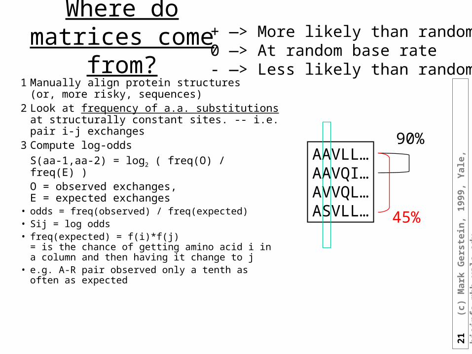
Where do matrices come from?
1 Manually align protein structures(or, more risky, sequences)
2 Look at frequency of a.a. substitutionsat structurally constant sites. -- i.e. pair i-j exchanges
3 Compute log-odds
S(aa-1,aa-2) = log2 ( freq(O) / freq(E) )O = observed exchanges, E = expected exchanges
• odds = freq(observed) / freq(expected)• Sij = log odds• freq(expected) = f(i)*f(j)
= is the chance of getting amino acid i in a column and then having it change to j
• e.g. A-R pair observed only a tenth as often as expected
+ —> More likely than random0 —> At random base rate- —> Less likely than random
AAVLL…AAVQI…AVVQL…ASVLL… 45%
90%
22
(c)
Mar
k G
erst
ein
, 19
99,
Yal
e, b
ioin
fo.m
bb
.yal
e.ed
u
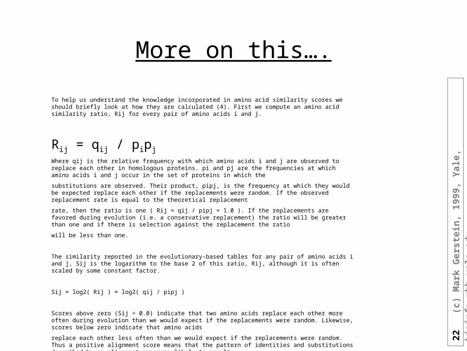
To help us understand the knowledge incorporated in amino acid similarity scores we should briefly look at how they are calculated (4). First we compute an amino acid similarity ratio, Rij for every pair of amino acids i and j.
Rij = qij / pipj
Where qij is the relative frequency with which amino acids i and j are observed to replace each other in homologous proteins. pi and pj are the frequencies at which amino acids i and j occur in the set of proteins in which the
substitutions are observed. Their product, pipj, is the frequency at which they would be expected replace each other if the replacements were random. If the observed replacement rate is equal to the theoretical replacement
rate, then the ratio is one ( Rij = qij / pipj = 1.0 ). If the replacements are favored during evolution (i.e. a conservative replacement) the ratio will be greater than one and if there is selection against the replacement the ratio
will be less than one.
The similarity reported in the evolutionary-based tables for any pair of amino acids i and j, Sij is the logarithm to the base 2 of this ratio, Rij, although it is often scaled by some constant factor.
Sij = log2( Rij ) = log2( qij / pipj )
Scores above zero (Sij > 0.0) indicate that two amino acids replace each other more often during evolution than we would expect if the replacements were random. Likewise, scores below zero indicate that amino acids
replace each other less often than we would expect if the replacements were random. Thus a positive alignment score means that the pattern of identities and substitutions described by an alignment are more likely to result
from previously observed evolutionary processes than to result from random replacements.
23
(c)
Mar
k G
erst
ein
, 19
99,
Yal
e, b
ioin
fo.m
bb
.yal
e.ed
u
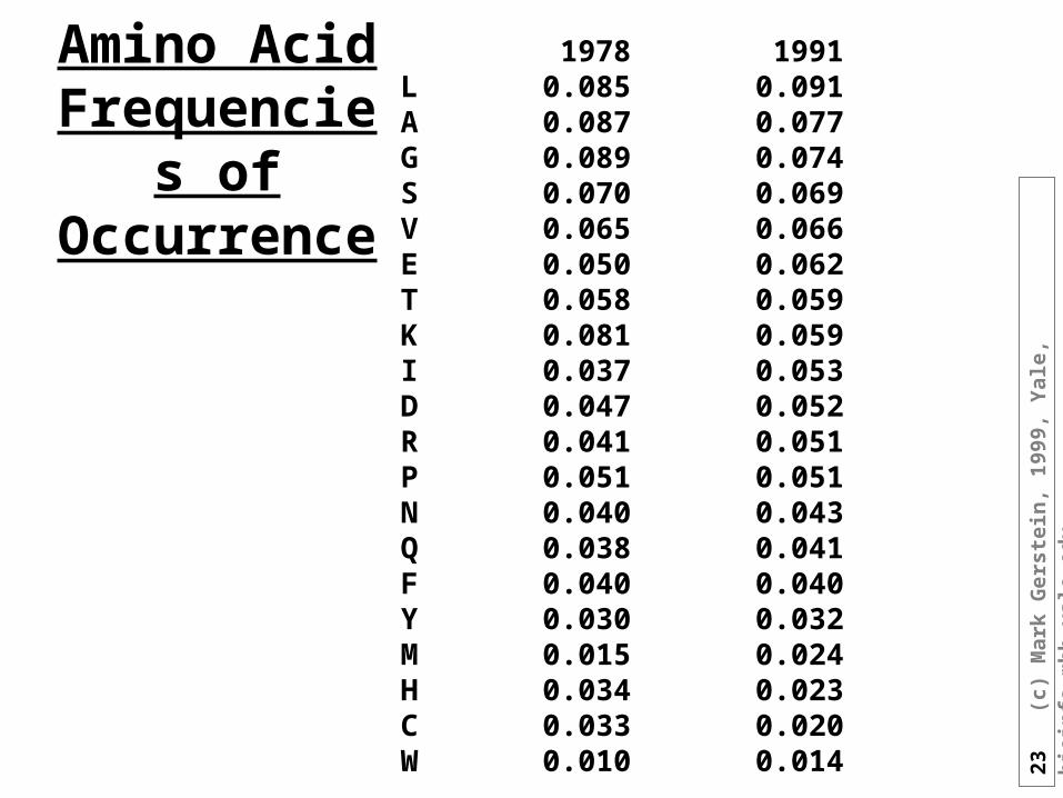
Amino Acid Frequencies
of Occurrence
1978 1991L 0.085 0.091A 0.087 0.077G 0.089 0.074S 0.070 0.069V 0.065 0.066E 0.050 0.062T 0.058 0.059K 0.081 0.059I 0.037 0.053D 0.047 0.052R 0.041 0.051P 0.051 0.051N 0.040 0.043Q 0.038 0.041F 0.040 0.040Y 0.030 0.032M 0.015 0.024H 0.034 0.023C 0.033 0.020W 0.010 0.014
24
(c)
Mar
k G
erst
ein
, 19
99,
Yal
e, b
ioin
fo.m
bb
.yal
e.ed
u
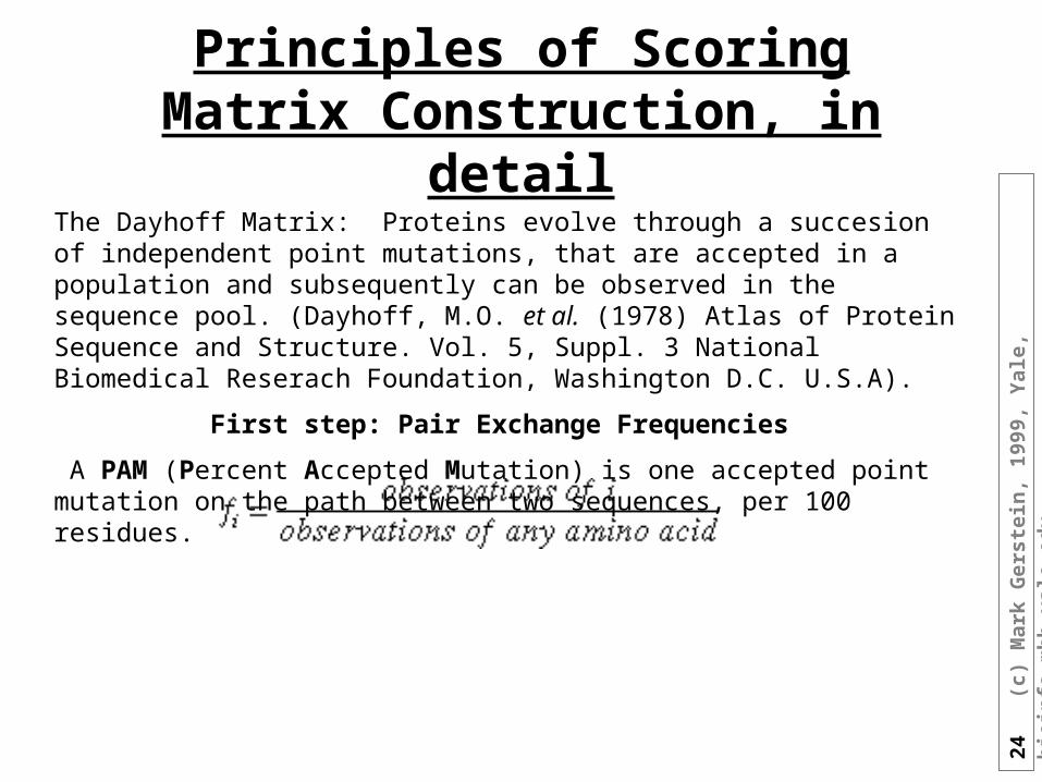
Principles of Scoring Matrix Construction, in detail
The Dayhoff Matrix: Proteins evolve through a succesion of independent point mutations, that are accepted in a population and subsequently can be observed in the sequence pool. (Dayhoff, M.O. et al. (1978) Atlas of Protein Sequence and Structure. Vol. 5, Suppl. 3 National Biomedical Reserach Foundation, Washington D.C. U.S.A).
First step: Pair Exchange Frequencies
A PAM (Percent Accepted Mutation) is one accepted point mutation on the path between two sequences, per 100 residues.
25
(c)
Mar
k G
erst
ein
, 19
99,
Yal
e, b
ioin
fo.m
bb
.yal
e.ed
u
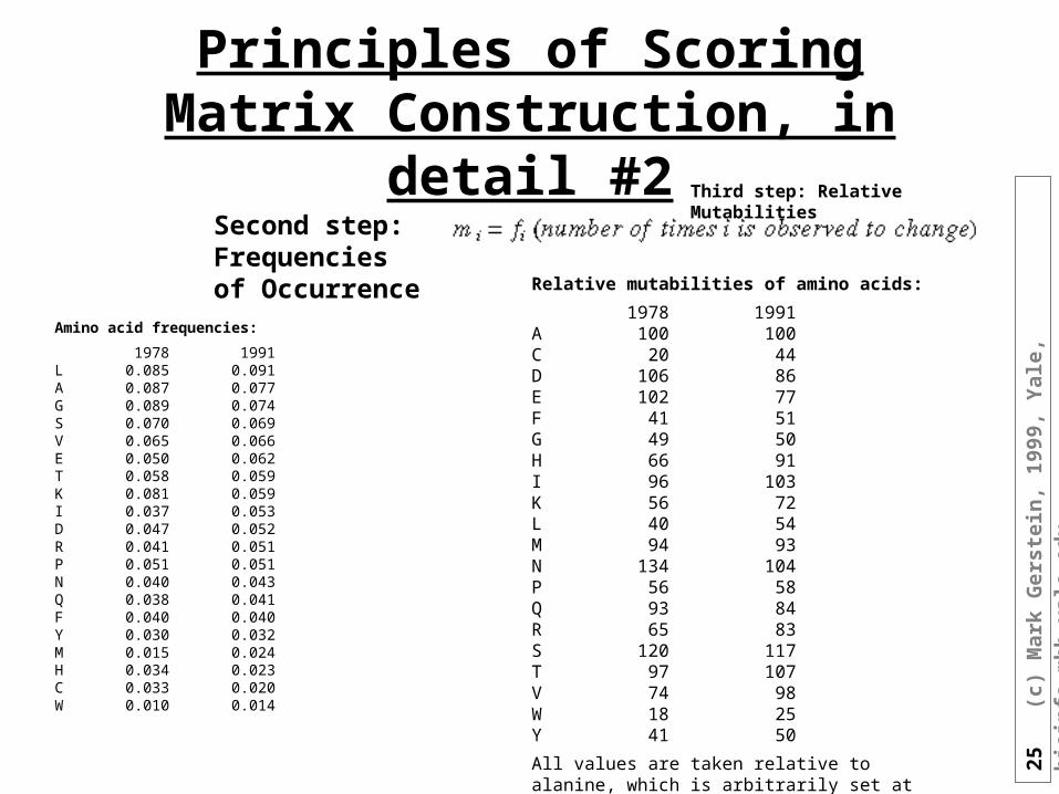
Principles of Scoring Matrix Construction, in detail #2Second step: Frequencies of Occurrence
Amino acid frequencies:
1978 1991L 0.085 0.091A 0.087 0.077G 0.089 0.074S 0.070 0.069V 0.065 0.066E 0.050 0.062T 0.058 0.059K 0.081 0.059I 0.037 0.053D 0.047 0.052R 0.041 0.051P 0.051 0.051N 0.040 0.043Q 0.038 0.041F 0.040 0.040Y 0.030 0.032M 0.015 0.024H 0.034 0.023C 0.033 0.020W 0.010 0.014
Third step: Relative Mutabilities
Relative mutabilities of amino acids:
1978 1991A 100 100C 20 44D 106 86E 102 77F 41 51G 49 50H 66 91I 96 103K 56 72L 40 54M 94 93N 134 104P 56 58Q 93 84R 65 83S 120 117T 97 107V 74 98W 18 25Y 41 50
All values are taken relative to alanine, which is arbitrarily set at 100.
26
(c)
Mar
k G
erst
ein
, 19
99,
Yal
e, b
ioin
fo.m
bb
.yal
e.ed
u
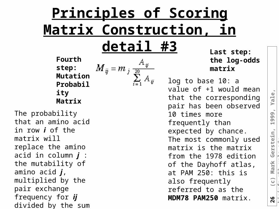
Principles of Scoring Matrix Construction, in detail #3Fourth step: Mutation Probability Matrix
The probability that an amino acid in row i of the matrix will replace the amino acid in column j : the mutability of amino acid j, multiplied by the pair exchange frequency for ij divided by the sum of all pair exchange frequencies for amino acid i:
Last step: the log-odds matrix
log to base 10: a value of +1 would mean that the corresponding pair has been observed 10 times more frequently than expected by chance. The most commonly used matrix is the matrix from the 1978 edition of the Dayhoff atlas, at PAM 250: this is also frequently referred to as the MDM78 PAM250 matrix.
27
(c)
Mar
k G
erst
ein
, 19
99,
Yal
e, b
ioin
fo.m
bb
.yal
e.ed
u
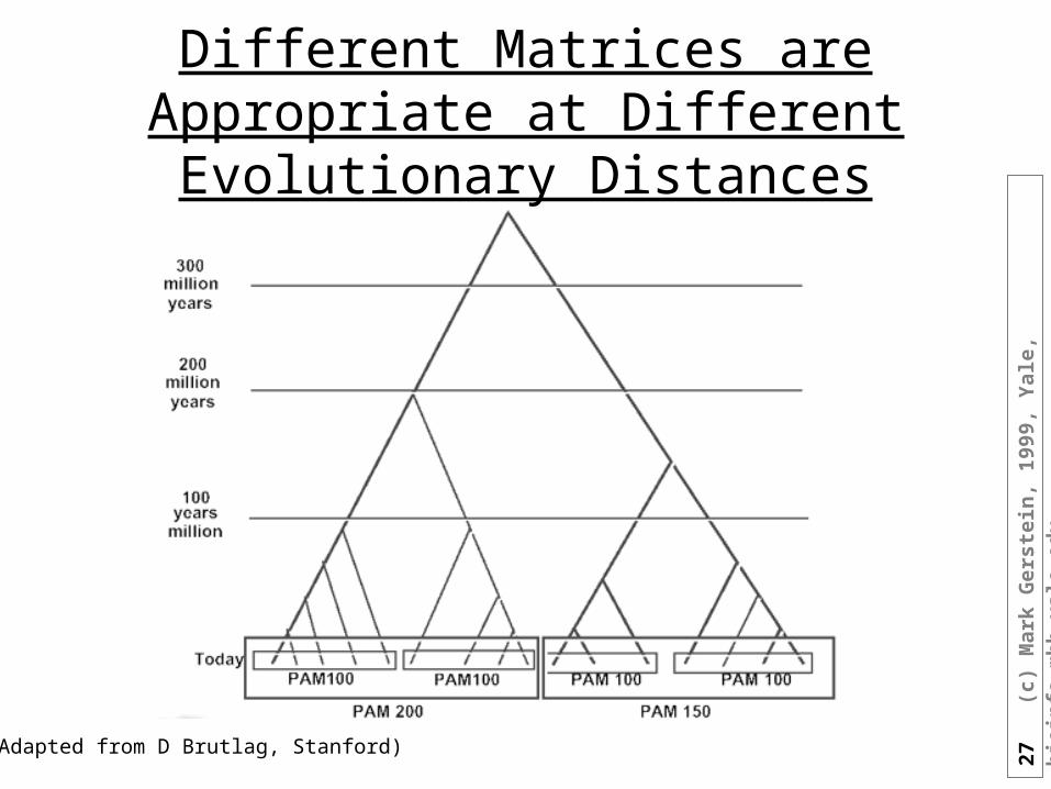
Different Matrices are Appropriate at Different Evolutionary Distances
(Adapted from D Brutlag, Stanford)
28
(c)
Mar
k G
erst
ein
, 19
99,
Yal
e, b
ioin
fo.m
bb
.yal
e.ed
u
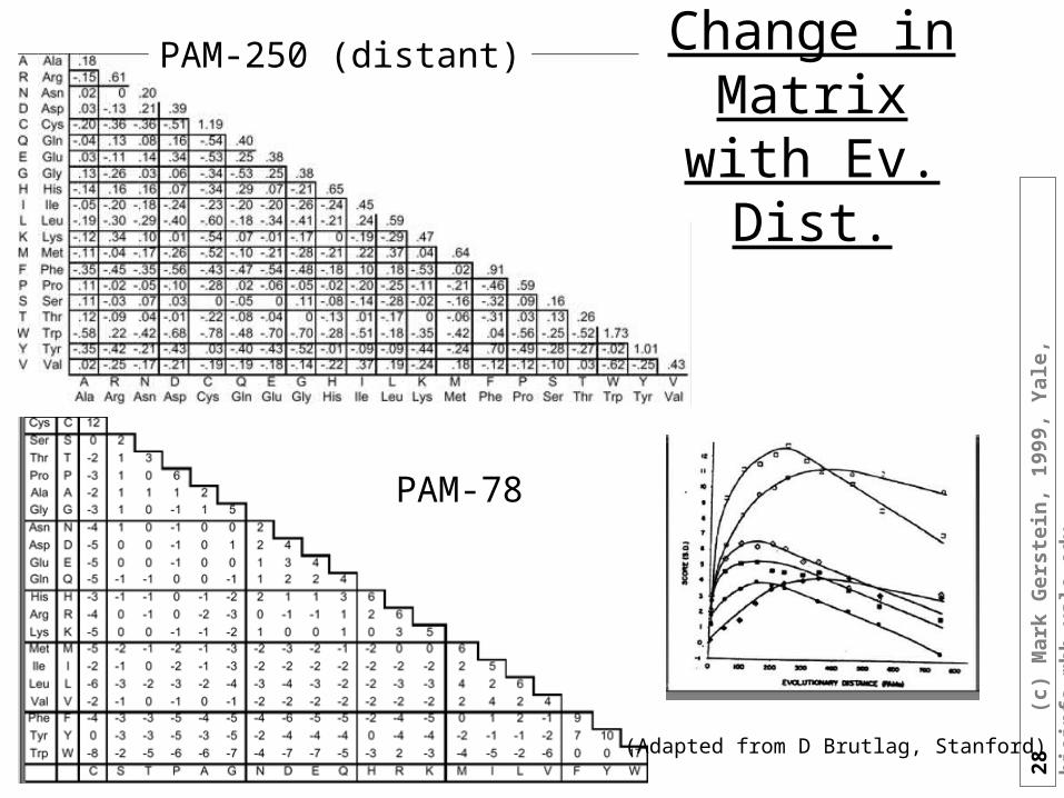
PAM-78
PAM-250 (distant) Change in Matrix with Ev. Dist.
(Adapted from D Brutlag, Stanford)
29
(c)
Mar
k G
erst
ein
, 19
99,
Yal
e, b
ioin
fo.m
bb
.yal
e.ed
u
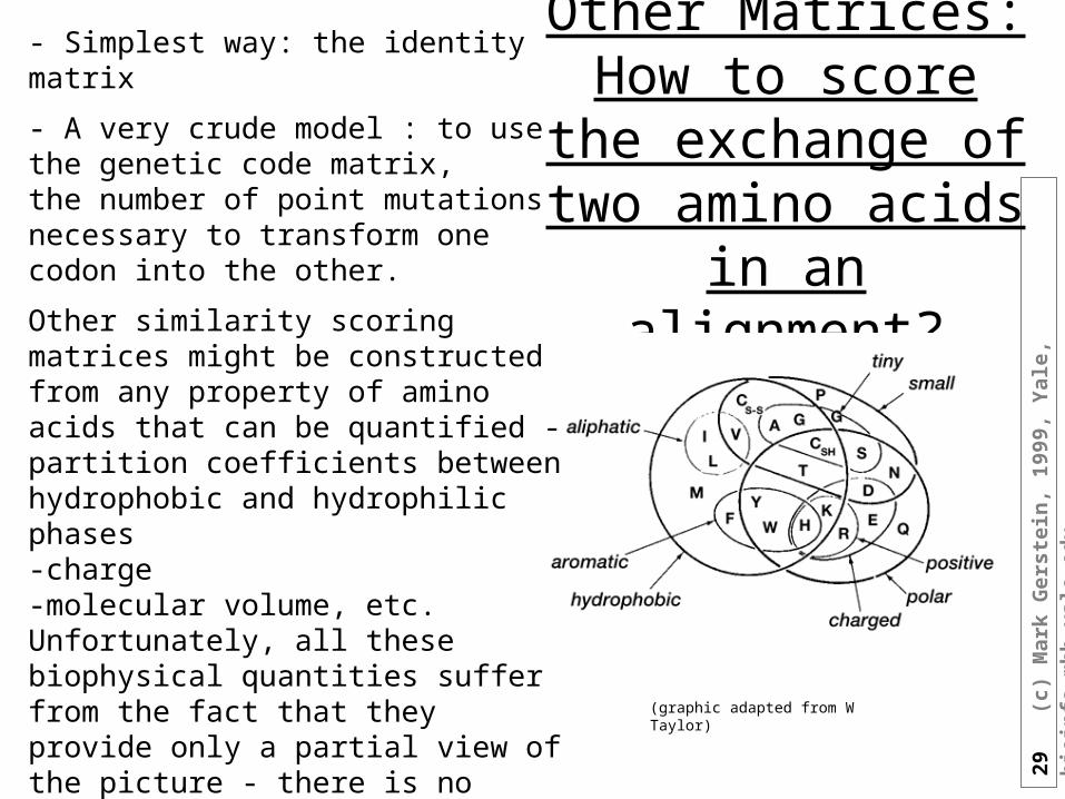
Other Matrices:How to score the exchange of two amino acids in an
alignment?
- Simplest way: the identity matrix
- A very crude model : to use the genetic code matrix, the number of point mutations necessary to transform one codon into the other.
Other similarity scoring matrices might be constructed from any property of amino acids that can be quantified -partition coefficients between hydrophobic and hydrophilic phases -charge -molecular volume, etc. Unfortunately, all these biophysical quantities suffer from the fact that they provide only a partial view of the picture - there is no guarantee, that any particular property is a good predictor for conservation of amino acids between related proteins.
(graphic adapted from W Taylor)
30
(c)
Mar
k G
erst
ein
, 19
99,
Yal
e, b
ioin
fo.m
bb
.yal
e.ed
u
The BLOSUM Matrices
Some concepts challenged: Are the evolutionary rates uniform over the whole of the protein sequence? (No.)
The BLOSUM matrices: Henikoff & Henikoff (Henikoff, S. & Henikoff J.G. (1992) PNAS 89:10915-10919) .
-Use blocks of sequence fragments from different protein families which can be aligned without the introduction of gaps. Amino acid pair frequencies can be compiled from these blocks
Different evolutionary distances are incorporated into this scheme with a clustering procedure: two sequences that are identical to each other for more than a certain threshold of positions are clustered.
More sequences are added to the cluster if they are identical to any sequence already in the cluster at the same level.
All sequences within a cluster are then simply averaged.
(A consequence of this clustering is that the contribution of closely related sequences to the frequency table is reduced, if the identity requirement is reduced. )
This leads to a series of matrices, analogous to the PAM series of matrices. BLOSUM80: derived at the 80% identity level.
BLOSUM62 is the BLAST default
31
(c)
Mar
k G
erst
ein
, 19
99,
Yal
e, b
ioin
fo.m
bb
.yal
e.ed
u
Local vs. Global Alignment
• GLOBAL = best alignment of entirety of both sequences For optimum global alignment, we want best score in the final row or final
column Are these sequences generally the same? Needleman Wunsch find alignment in which total score is highest, perhaps at expense of areas
of great local similarity
• LOCAL = best alignment of segments, without regard to rest of sequence For optimum local alignment, we want best score anywhere in matrix (will
discuss) Do these two sequences contain high scoring subsequences Smith Waterman find alignment in which the highest scoring subsequences are identified,
at the expense of the overall score
(Adapted from R Altman)
32
(c)
Mar
k G
erst
ein
, 19
99,
Yal
e, b
ioin
fo.m
bb
.yal
e.ed
u
Modifications for Local Alignment
1. The scoring system uses negative scores for mismatches
2. The minimum score for [i,j] is zero
3. The best score anywhere in the matrix (not just last column or row)
• These three changes cause the algorithm to seek high scoring subsequences, which are not penalized for their global effects (mod. 1), which don’t include areas of poor match (mod. 2), and which can occur anywhere (mod. 3)
(Adapted from R Altman)

33
(c)
Mar
k G
erst
ein
, 19
99,
Yal
e, b
ioin
fo.m
bb
.yal
e.ed
u
End of Class 1
34
(c)
Mar
k G
erst
ein
, 19
99,
Yal
e, b
ioin
fo.m
bb
.yal
e.ed
u
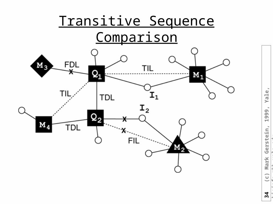
Transitive Sequence Comparison
35
(c)
Mar
k G
erst
ein
, 19
99,
Yal
e, b
ioin
fo.m
bb
.yal
e.ed
u
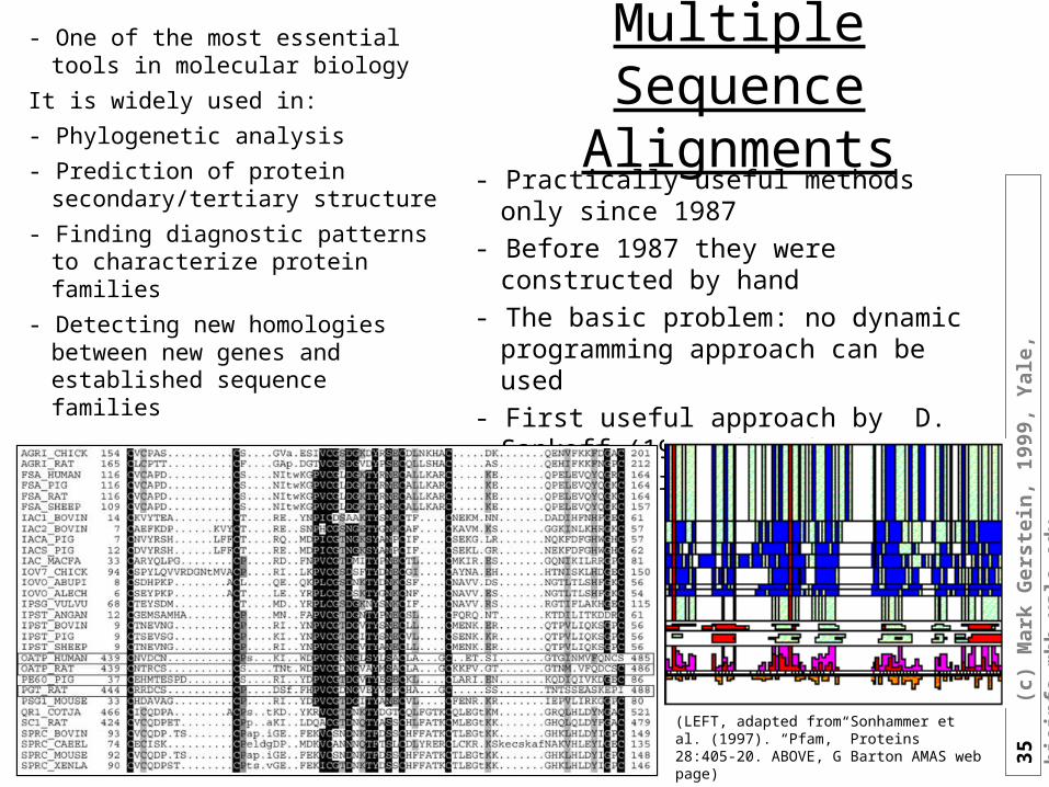
Multiple Sequence Alignments
- One of the most essential tools in molecular biology
It is widely used in:
- Phylogenetic analysis
- Prediction of protein secondary/tertiary structure
- Finding diagnostic patterns to characterize protein families
- Detecting new homologies between new genes and established sequence families
- Practically useful methods only since 1987
- Before 1987 they were constructed by hand
- The basic problem: no dynamic programming approach can be used
- First useful approach by D. Sankoff (1987) based on phylogenetics
(LEFT, adapted from Sonhammer et al. (1997). “Pfam,” Proteins 28:405-20. ABOVE, G Barton AMAS web page)
36
(c)
Mar
k G
erst
ein
, 19
99,
Yal
e, b
ioin
fo.m
bb
.yal
e.ed
u
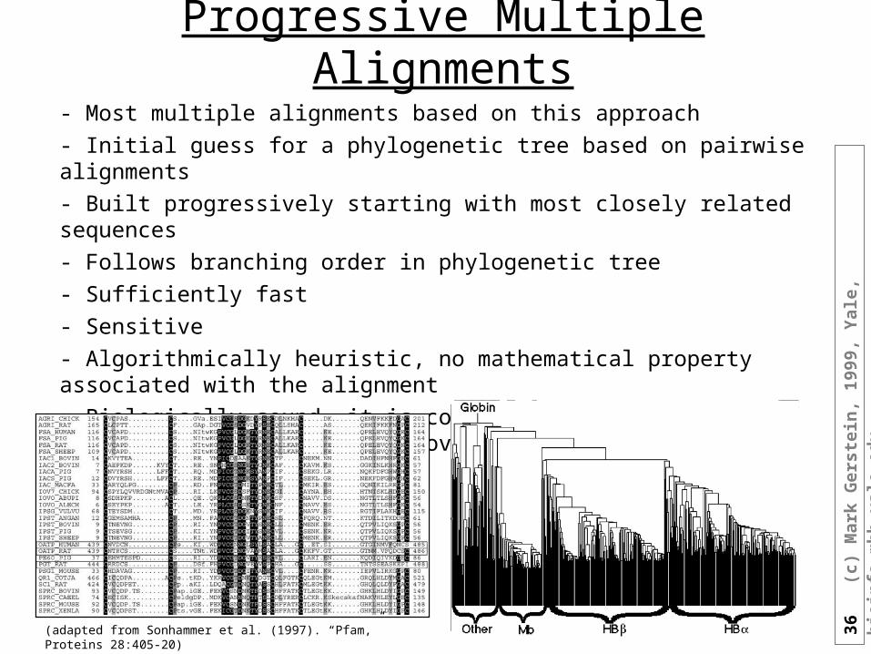
Progressive Multiple Alignments
- Most multiple alignments based on this approach
- Initial guess for a phylogenetic tree based on pairwise alignments
- Built progressively starting with most closely related sequences
- Follows branching order in phylogenetic tree
- Sufficiently fast
- Sensitive
- Algorithmically heuristic, no mathematical property associated with the alignment
- Biologically sound, it is common to derive alignments which are impossible to improve by eye
(adapted from Sonhammer et al. (1997). “Pfam,” Proteins 28:405-20)

37
(c)
Mar
k G
erst
ein
, 19
99,
Yal
e, b
ioin
fo.m
bb
.yal
e.ed
u
Problems with Progressive Alignments
- Local Minimum Problem - Parameter Choice Problem
1. Local Minimum Problem
- It stems from greedy nature of alignment (mistakes made early in alignment cannot be corrected later)
- A better tree gives a better alignment (UPGMA neighbour-joining tree method)
2. Parameter Choice Problem
• - It stems from using just one set of parameters (and hoping that they will do for all)
38
(c)
Mar
k G
erst
ein
, 19
99,
Yal
e, b
ioin
fo.m
bb
.yal
e.ed
u
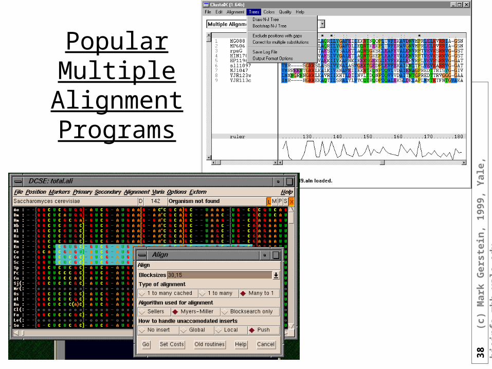
Popular Multiple
Alignment Programs
39
(c)
Mar
k G
erst
ein
, 19
99,
Yal
e, b
ioin
fo.m
bb
.yal
e.ed
u
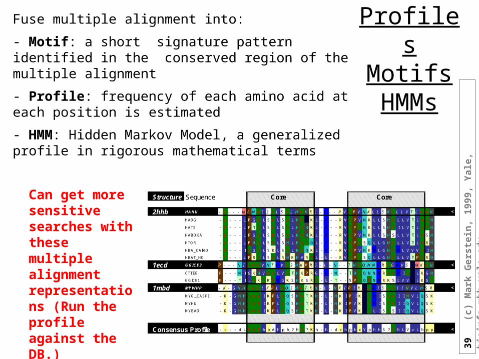
Profiles MotifsHMMs
Fuse multiple alignment into:
- Motif: a short signature pattern identified in the conserved region of the multiple alignment
- Profile: frequency of each amino acid at each position is estimated
- HMM: Hidden Markov Model, a generalized profile in rigorous mathematical terms
Structure Sequence Core Core
2hhb HAHU - D - - - M P N A L S A L S D L H A H K L - F - - R V D P V N K L L S H C L L V T L A A H <
HADG - D - - - L P G A L S A L S D L H A Y K L - F - - R V D P V N K L L S H C L L V T L A C H
HATS - D - - - L P T A L S A L S D L H A H K L - F - - R V D P A N K L L S H C I L V T L A C H
HABOKA - D - - - L P G A L S D L S D L H A H K L - F - - R V D P V N K L L S H S L L V T L A S H
HTOR - D - - - L P H A L S A L S H L H A C Q L - F - - R V D P A S Q L L G H C L L V T L A R H
HBA_CAIMO - D - - - I A G A L S K L S D L H A Q K L - F - - R V D P V N K F L G H C F L V V V A I H
HBAT_HO - E - - - L P R A L S A L R H R H V R E L - L - - R V D P A S Q L L G H C L L V T P A R H
1ecd GGICE3 P - - - N I E A D V N T F V A S H K P R G - L - N - - T H D Q N N F R A G F V S Y M K A H <
CTTEE P - - - N I G K H V D A L V A T H K P R G - F - N - - T H A Q N N F R A A F I A Y L K G H
GGICE1 P - - - T I L A K A K D F G K S H K S R A - L - T - - S P A Q D N F R K S L V V Y L K G A
1mbd MYWHP - K - G H H E A E L K P L A Q S H A T K H - L - H K I P I K Y E F I S E A I I H V L H S R <
MYG_CASFI - K - G H H E A E I K P L A Q S H A T K H - L - H K I P I K Y E F I S E A I I H V L Q S K
MYHU - K - G H H E A E I K P L A Q S H A T K H - L - H K I P V K Y E F I S E C I I Q V L Q S K
MYBAO - K - G H H E A E I K P L A Q S H A T K H - L - H K I P V K Y E L I S E S I I Q V L Q S K
Consensus Profile - c - - d L P A E h p A h p h ? H A ? K h - h - d c h p h c Y p h h S ? C h L V v L h p p <
Can get more sensitive searches with these multiple alignment representations (Run the profile against the DB.)
40
(c)
Mar
k G
erst
ein
, 19
99,
Yal
e, b
ioin
fo.m
bb
.yal
e.ed
u
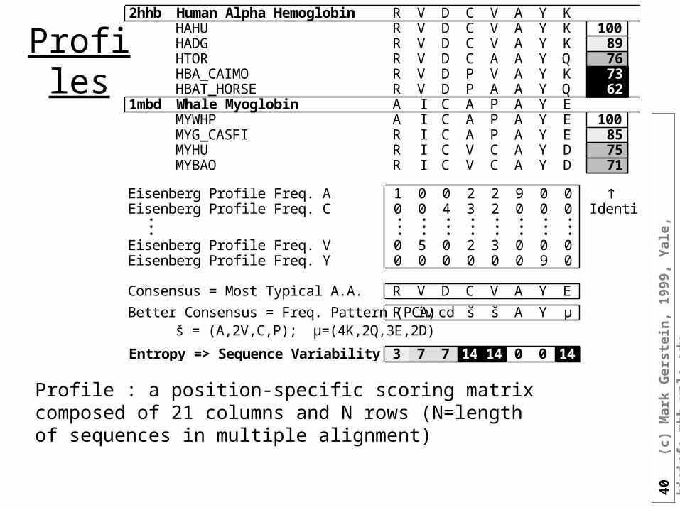
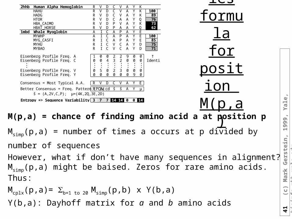
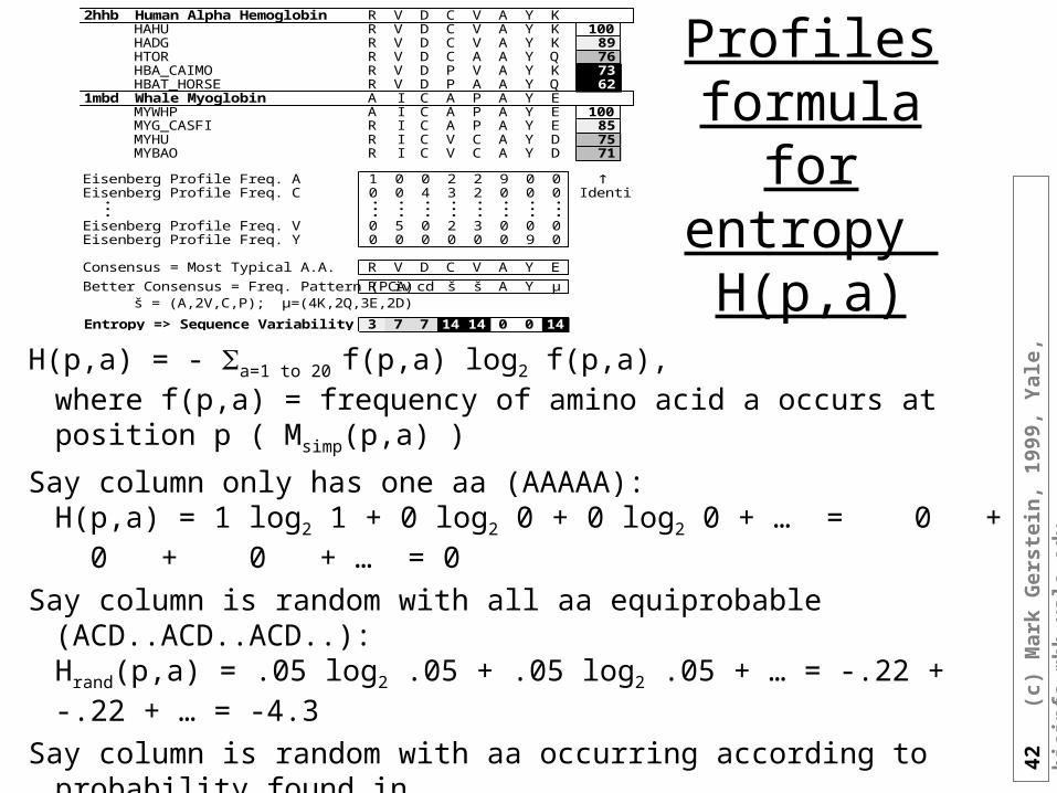
Profiles
2hhb Human Alpha Hemoglobin R V D C V A Y KHAHU R V D C V A Y K 100HADG R V D C V A Y K 89HTOR R V D C A A Y Q 76HBA_CAIMO R V D P V A Y K 73HBAT_HORSE R V D P A A Y Q 62
1mbd Whale Myoglobin A I C A P A Y EMYWHP A I C A P A Y E 100MYG_CASFI R I C A P A Y E 85MYHU R I C V C A Y D 75MYBAO R I C V C A Y D 71
Eisenberg Profile Freq. A 1 0 0 2 2 9 0 0 Eisenberg Profile Freq. C 0 0 4 3 2 0 0 0 Identity. . . . . . . . .. . . . . . . . .. . . . . . . . .Eisenberg Profile Freq. V 0 5 0 2 3 0 0 0Eisenberg Profile Freq. Y 0 0 0 0 0 0 9 0
Consensus = Most Typical A.A. R V D C V A Y E
Better Consensus = Freq. Pattern (PCA) R iv cd š š A Y µš = (A,2V,C,P); µ=(4K,2Q,3E,2D)
Entropy => Sequence Variability 3 7 7 14 14 0 0 14
Profile : a position-specific scoring matrix composed of 21 columns and N rows (N=length of sequences in multiple alignment)
41
(c)
Mar
k G
erst
ein
, 19
99,
Yal
e, b
ioin
fo.m
bb
.yal
e.ed
u
Profiles formula
for position
M(p,a)
2hhb Human Alpha Hemoglobin R V D C V A Y KHAHU R V D C V A Y K 100HADG R V D C V A Y K 89HTOR R V D C A A Y Q 76HBA_CAIMO R V D P V A Y K 73HBAT_HORSE R V D P A A Y Q 62
1mbd Whale Myoglobin A I C A P A Y EMYWHP A I C A P A Y E 100MYG_CASFI R I C A P A Y E 85MYHU R I C V C A Y D 75MYBAO R I C V C A Y D 71
Eisenberg Profile Freq. A 1 0 0 2 2 9 0 0 Eisenberg Profile Freq. C 0 0 4 3 2 0 0 0 Identity. . . . . . . . .. . . . . . . . .. . . . . . . . .Eisenberg Profile Freq. V 0 5 0 2 3 0 0 0Eisenberg Profile Freq. Y 0 0 0 0 0 0 9 0
Consensus = Most Typical A.A. R V D C V A Y E
Better Consensus = Freq. Pattern (PCA) R iv cd š š A Y µš = (A,2V,C,P); µ=(4K,2Q,3E,2D)
Entropy => Sequence Variability 3 7 7 14 14 0 0 14
M(p,a) = chance of finding amino acid a at position p
Msimp(p,a) = number of times a occurs at p divided by number of sequences
However, what if don’t have many sequences in alignment? Msimp(p,a) might be baised. Zeros for rare amino acids. Thus:
Mcplx(p,a)= b=1 to 20 Msimp(p,b) x Y(b,a)
Y(b,a): Dayhoff matrix for a and b amino acids
S(p,a) ~ a=1 to 20 Msimp(p,a) ln Msimp(p,a)
42
(c)
Mar
k G
erst
ein
, 19
99,
Yal
e, b
ioin
fo.m
bb
.yal
e.ed
u
Profiles formula for
entropy H(p,a)
2hhb Human Alpha Hemoglobin R V D C V A Y KHAHU R V D C V A Y K 100HADG R V D C V A Y K 89HTOR R V D C A A Y Q 76HBA_CAIMO R V D P V A Y K 73HBAT_HORSE R V D P A A Y Q 62
1mbd Whale Myoglobin A I C A P A Y EMYWHP A I C A P A Y E 100MYG_CASFI R I C A P A Y E 85MYHU R I C V C A Y D 75MYBAO R I C V C A Y D 71
Eisenberg Profile Freq. A 1 0 0 2 2 9 0 0 Eisenberg Profile Freq. C 0 0 4 3 2 0 0 0 Identity. . . . . . . . .. . . . . . . . .. . . . . . . . .Eisenberg Profile Freq. V 0 5 0 2 3 0 0 0Eisenberg Profile Freq. Y 0 0 0 0 0 0 9 0
Consensus = Most Typical A.A. R V D C V A Y E
Better Consensus = Freq. Pattern (PCA) R iv cd š š A Y µš = (A,2V,C,P); µ=(4K,2Q,3E,2D)
Entropy => Sequence Variability 3 7 7 14 14 0 0 14
H(p,a) = - a=1 to 20 f(p,a) log2 f(p,a),
where f(p,a) = frequency of amino acid a occurs at position p ( Msimp(p,a) )
Say column only has one aa (AAAAA): H(p,a) = 1 log2 1 + 0 log2 0 + 0 log2 0 + … = 0 + 0 + 0 + … = 0
Say column is random with all aa equiprobable (ACD..ACD..ACD..):Hrand(p,a) = .05 log2 .05 + .05 log2 .05 + … = -.22 + -.22 + … = -4.3
Say column is random with aa occurring according to probability found inthe sequence databases (ACAAAADAADDDDAAAA….):Hdb(a) = - a=1 to 20
F(a) log2 F(a), where F(a) is freq. of occurrence of a in DB
Hcorrected(p,a) = H(p,a) – Hdb(a)
43
(c)
Mar
k G
erst
ein
, 19
99,
Yal
e, b
ioin
fo.m
bb
.yal
e.ed
u
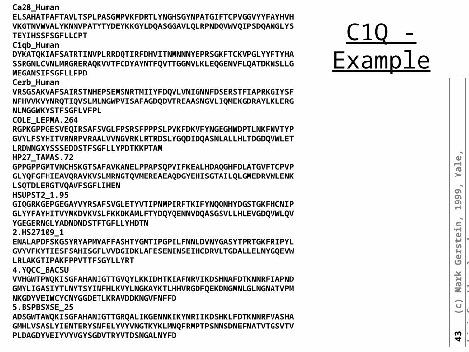
C1Q - Example
Ca28_Human ELSAHATPAFTAVLTSPLPASGMPVKFDRTLYNGHSGYNPATGIFTCPVGGVYYFAYHVH VKGTNVWVALYKNNVPATYTYDEYKKGYLDQASGGAVLQLRPNDQVWVQIPSDQANGLYS TEYIHSSFSGFLLCPT C1qb_Human DYKATQKIAFSATRTINVPLRRDQTIRFDHVITNMNNNYEPRSGKFTCKVPGLYYFTYHA SSRGNLCVNLMRGRERAQKVVTFCDYAYNTFQVTTGGMVLKLEQGENVFLQATDKNSLLG MEGANSIFSGFLLFPD Cerb_Human VRSGSAKVAFSAIRSTNHEPSEMSNRTMIIYFDQVLVNIGNNFDSERSTFIAPRKGIYSF NFHVVKVYNRQTIQVSLMLNGWPVISAFAGDQDVTREAASNGVLIQMEKGDRAYLKLERG NLMGGWKYSTFSGFLVFPL COLE_LEPMA.264 RGPKGPPGESVEQIRSAFSVGLFPSRSFPPPSLPVKFDKVFYNGEGHWDPTLNKFNVTYP GVYLFSYHITVRNRPVRAALVVNGVRKLRTRDSLYGQDIDQASNLALLHLTDGDQVWLET LRDWNGXYSSSEDDSTFSGFLLYPDTKKPTAM HP27_TAMAS.72 GPPGPPGMTVNCHSKGTSAFAVKANELPPAPSQPVIFKEALHDAQGHFDLATGVFTCPVP GLYQFGFHIEAVQRAVKVSLMRNGTQVMEREAEAQDGYEHISGTAILQLGMEDRVWLENK LSQTDLERGTVQAVFSGFLIHEN HSUPST2_1.95 GIQGRKGEPGEGAYVYRSAFSVGLETYVTIPNMPIRFTKIFYNQQNHYDGSTGKFHCNIP GLYYFAYHITVYMKDVKVSLFKKDKAMLFTYDQYQENNVDQASGSVLLHLEVGDQVWLQV YGEGERNGLYADNDNDSTFTGFLLYHDTN 2.HS27109_1 ENALAPDFSKGSYRYAPMVAFFASHTYGMTIPGPILFNNLDVNYGASYTPRTGKFRIPYL GVYVFKYTIESFSAHISGFLVVDGIDKLAFESENINSEIHCDRVLTGDALLELNYGQEVW LRLAKGTIPAKFPPVTTFSGYLLYRT 4.YQCC_BACSU VVHGWTPWQKISGFAHANIGTTGVQYLKKIDHTKIAFNRVIKDSHNAFDTKNNRFIAPND GMYLIGASIYTLNYTSYINFHLKVYLNGKAYKTLHHVRGDFQEKDNGMNLGLNGNATVPM NKGDYVEIWCYCNYGGDETLKRAVDDKNGVFNFFD 5.BSPBSXSE_25 ADSGWTAWQKISGFAHANIGTTGRQALIKGENNKIKYNRIIKDSHKLFDTKNNRFVASHA GMHLVSASLYIENTERYSNFELYVYVNGTKYKLMNQFRMPTPSNNSDNEFNATVTGSVTV PLDAGDYVEIYVYVGYSGDVTRYVTDSNGALNYFD
44
(c)
Mar
k G
erst
ein
, 19
99,
Yal
e, b
ioin
fo.m
bb
.yal
e.ed
u
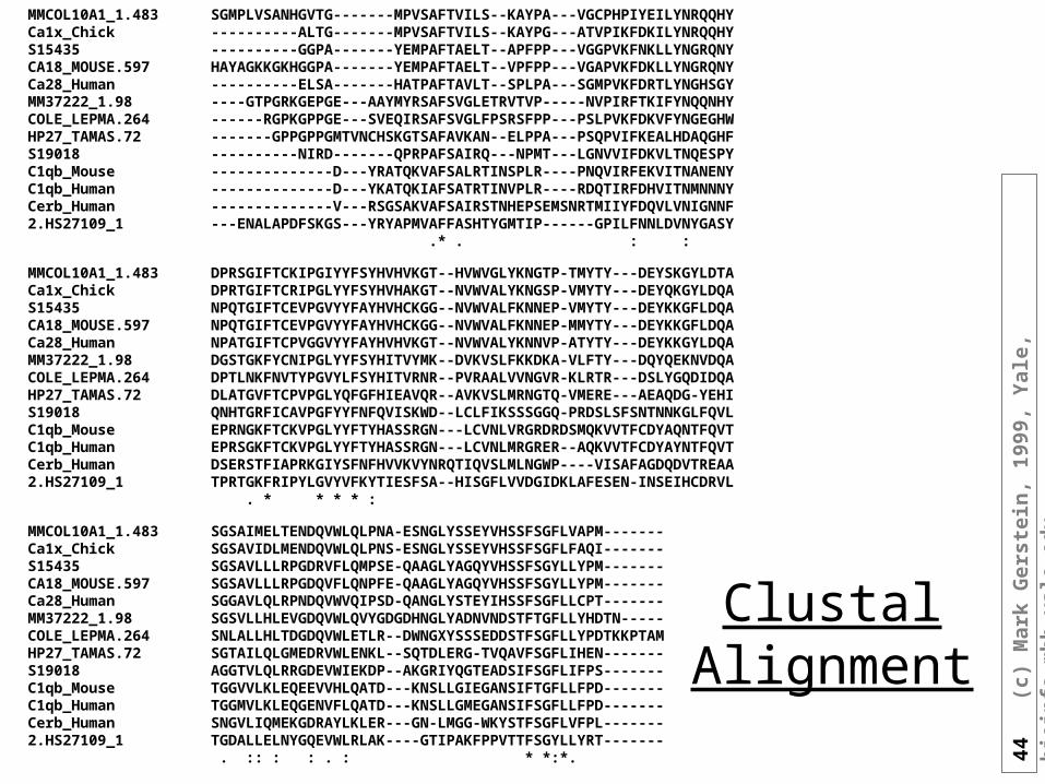
Clustal Alignment
MMCOL10A1_1.483 SGMPLVSANHGVTG-------MPVSAFTVILS--KAYPA---VGCPHPIYEILYNRQQHY Ca1x_Chick ----------ALTG-------MPVSAFTVILS--KAYPG---ATVPIKFDKILYNRQQHY S15435 ----------GGPA-------YEMPAFTAELT--APFPP---VGGPVKFNKLLYNGRQNY CA18_MOUSE.597 HAYAGKKGKHGGPA-------YEMPAFTAELT--VPFPP---VGAPVKFDKLLYNGRQNY Ca28_Human ----------ELSA-------HATPAFTAVLT--SPLPA---SGMPVKFDRTLYNGHSGY MM37222_1.98 ----GTPGRKGEPGE---AAYMYRSAFSVGLETRVTVP-----NVPIRFTKIFYNQQNHY COLE_LEPMA.264 ------RGPKGPPGE---SVEQIRSAFSVGLFPSRSFPP---PSLPVKFDKVFYNGEGHW HP27_TAMAS.72 -------GPPGPPGMTVNCHSKGTSAFAVKAN--ELPPA---PSQPVIFKEALHDAQGHF S19018 ----------NIRD-------QPRPAFSAIRQ---NPMT---LGNVVIFDKVLTNQESPY C1qb_Mouse --------------D---YRATQKVAFSALRTINSPLR----PNQVIRFEKVITNANENY C1qb_Human --------------D---YKATQKIAFSATRTINVPLR----RDQTIRFDHVITNMNNNY Cerb_Human --------------V---RSGSAKVAFSAIRSTNHEPSEMSNRTMIIYFDQVLVNIGNNF 2.HS27109_1 ---ENALAPDFSKGS---YRYAPMVAFFASHTYGMTIP------GPILFNNLDVNYGASY .* . : :
MMCOL10A1_1.483 DPRSGIFTCKIPGIYYFSYHVHVKGT--HVWVGLYKNGTP-TMYTY---DEYSKGYLDTA Ca1x_Chick DPRTGIFTCRIPGLYYFSYHVHAKGT--NVWVALYKNGSP-VMYTY---DEYQKGYLDQA S15435 NPQTGIFTCEVPGVYYFAYHVHCKGG--NVWVALFKNNEP-VMYTY---DEYKKGFLDQA CA18_MOUSE.597 NPQTGIFTCEVPGVYYFAYHVHCKGG--NVWVALFKNNEP-MMYTY---DEYKKGFLDQA Ca28_Human NPATGIFTCPVGGVYYFAYHVHVKGT--NVWVALYKNNVP-ATYTY---DEYKKGYLDQA MM37222_1.98 DGSTGKFYCNIPGLYYFSYHITVYMK--DVKVSLFKKDKA-VLFTY---DQYQEKNVDQA COLE_LEPMA.264 DPTLNKFNVTYPGVYLFSYHITVRNR--PVRAALVVNGVR-KLRTR---DSLYGQDIDQA HP27_TAMAS.72 DLATGVFTCPVPGLYQFGFHIEAVQR--AVKVSLMRNGTQ-VMERE---AEAQDG-YEHI S19018 QNHTGRFICAVPGFYYFNFQVISKWD--LCLFIKSSSGGQ-PRDSLSFSNTNNKGLFQVL C1qb_Mouse EPRNGKFTCKVPGLYYFTYHASSRGN---LCVNLVRGRDRDSMQKVVTFCDYAQNTFQVT C1qb_Human EPRSGKFTCKVPGLYYFTYHASSRGN---LCVNLMRGRER--AQKVVTFCDYAYNTFQVT Cerb_Human DSERSTFIAPRKGIYSFNFHVVKVYNRQTIQVSLMLNGWP----VISAFAGDQDVTREAA 2.HS27109_1 TPRTGKFRIPYLGVYVFKYTIESFSA--HISGFLVVDGIDKLAFESEN-INSEIHCDRVL . * * * * :
MMCOL10A1_1.483 SGSAIMELTENDQVWLQLPNA-ESNGLYSSEYVHSSFSGFLVAPM------- Ca1x_Chick SGSAVIDLMENDQVWLQLPNS-ESNGLYSSEYVHSSFSGFLFAQI------- S15435 SGSAVLLLRPGDRVFLQMPSE-QAAGLYAGQYVHSSFSGYLLYPM------- CA18_MOUSE.597 SGSAVLLLRPGDQVFLQNPFE-QAAGLYAGQYVHSSFSGYLLYPM------- Ca28_Human SGGAVLQLRPNDQVWVQIPSD-QANGLYSTEYIHSSFSGFLLCPT------- MM37222_1.98 SGSVLLHLEVGDQVWLQVYGDGDHNGLYADNVNDSTFTGFLLYHDTN----- COLE_LEPMA.264 SNLALLHLTDGDQVWLETLR--DWNGXYSSSEDDSTFSGFLLYPDTKKPTAM HP27_TAMAS.72 SGTAILQLGMEDRVWLENKL--SQTDLERG-TVQAVFSGFLIHEN------- S19018 AGGTVLQLRRGDEVWIEKDP--AKGRIYQGTEADSIFSGFLIFPS------- C1qb_Mouse TGGVVLKLEQEEVVHLQATD---KNSLLGIEGANSIFTGFLLFPD------- C1qb_Human TGGMVLKLEQGENVFLQATD---KNSLLGMEGANSIFSGFLLFPD------- Cerb_Human SNGVLIQMEKGDRAYLKLER---GN-LMGG-WKYSTFSGFLVFPL------- 2.HS27109_1 TGDALLELNYGQEVWLRLAK----GTIPAKFPPVTTFSGYLLYRT------- . :: : : . : * *:*.
45
(c)
Mar
k G
erst
ein
, 19
99,
Yal
e, b
ioin
fo.m
bb
.yal
e.ed
u
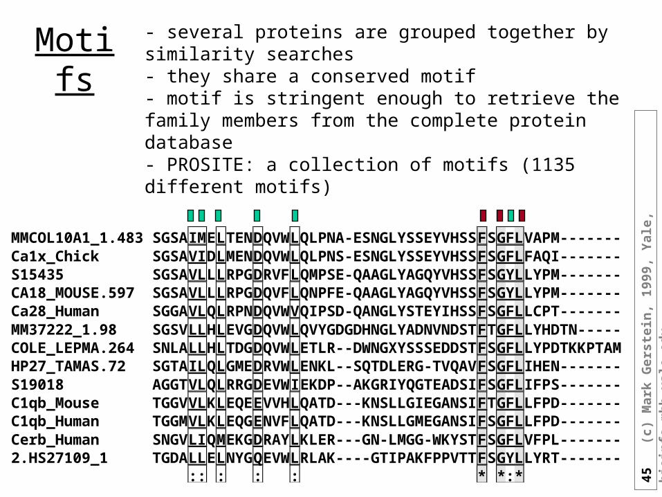
- several proteins are grouped together by similarity searches - they share a conserved motif - motif is stringent enough to retrieve the family members from the complete protein database - PROSITE: a collection of motifs (1135 different motifs)
Motifs
MMCOL10A1_1.483 SGSAIMELTENDQVWLQLPNA-ESNGLYSSEYVHSSFSGFLVAPM-------Ca1x_Chick SGSAVIDLMENDQVWLQLPNS-ESNGLYSSEYVHSSFSGFLFAQI-------S15435 SGSAVLLLRPGDRVFLQMPSE-QAAGLYAGQYVHSSFSGYLLYPM-------CA18_MOUSE.597 SGSAVLLLRPGDQVFLQNPFE-QAAGLYAGQYVHSSFSGYLLYPM-------Ca28_Human SGGAVLQLRPNDQVWVQIPSD-QANGLYSTEYIHSSFSGFLLCPT-------MM37222_1.98 SGSVLLHLEVGDQVWLQVYGDGDHNGLYADNVNDSTFTGFLLYHDTN-----COLE_LEPMA.264 SNLALLHLTDGDQVWLETLR--DWNGXYSSSEDDSTFSGFLLYPDTKKPTAMHP27_TAMAS.72 SGTAILQLGMEDRVWLENKL--SQTDLERG-TVQAVFSGFLIHEN-------S19018 AGGTVLQLRRGDEVWIEKDP--AKGRIYQGTEADSIFSGFLIFPS-------C1qb_Mouse TGGVVLKLEQEEVVHLQATD---KNSLLGIEGANSIFTGFLLFPD-------C1qb_Human TGGMVLKLEQGENVFLQATD---KNSLLGMEGANSIFSGFLLFPD-------Cerb_Human SNGVLIQMEKGDRAYLKLER---GN-LMGG-WKYSTFSGFLVFPL-------2.HS27109_1 TGDALLELNYGQEVWLRLAK----GTIPAKFPPVTTFSGYLLYRT------- :: : : : * *:*
46
(c)
Mar
k G
erst
ein
, 19
99,
Yal
e, b
ioin
fo.m
bb
.yal
e.ed
u
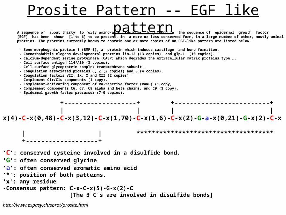
Prosite Pattern -- EGF like patternA sequence of about thirty to forty amino-acid residues long found in the sequence of epidermal growth factor (EGF) has been shown [1 to 6] to be present, in a more or less conserved form, in a large number of other, mostly animal proteins. The proteins currently known to contain one or more copies of an EGF-like pattern are listed below.
- Bone morphogenic protein 1 (BMP-1), a protein which induces cartilage and bone formation. - Caenorhabditis elegans developmental proteins lin-12 (13 copies) and glp-1 (10 copies). - Calcium-dependent serine proteinase (CASP) which degrades the extracellular matrix proteins type …. - Cell surface antigen 114/A10 (3 copies). - Cell surface glycoprotein complex transmembrane subunit . - Coagulation associated proteins C, Z (2 copies) and S (4 copies). - Coagulation factors VII, IX, X and XII (2 copies). - Complement C1r/C1s components (1 copy). - Complement-activating component of Ra-reactive factor (RARF) (1 copy). - Complement components C6, C7, C8 alpha and beta chains, and C9 (1 copy). - Epidermal growth factor precursor (7-9 copies).
+-------------------+ +-------------------------+ | | | | x(4)-C-x(0,48)-C-x(3,12)-C-x(1,70)-C-x(1,6)-C-x(2)-G-a-x(0,21)-G-x(2)-C-x
| | ************************************ +-------------------+
'C': conserved cysteine involved in a disulfide bond.'G': often conserved glycine'a': often conserved aromatic amino acid'*': position of both patterns.'x': any residue-Consensus pattern: C-x-C-x(5)-G-x(2)-C [The 3 C's are involved in disulfide bonds]
http://www.expasy.ch/sprot/prosite.html
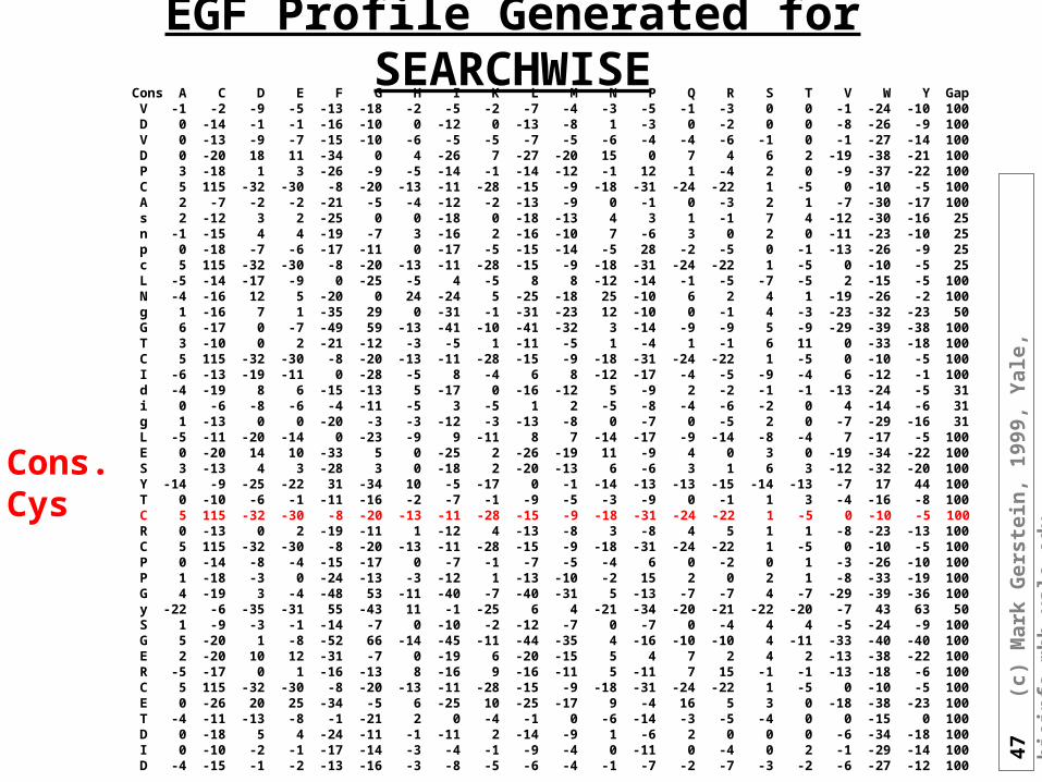
47
(c)
Mar
k G
erst
ein
, 19
99,
Yal
e, b
ioin
fo.m
bb
.yal
e.ed
u
EGF Profile Generated for SEARCHWISECons A C D E F G H I K L M N P Q R S T V W Y Gap V -1 -2 -9 -5 -13 -18 -2 -5 -2 -7 -4 -3 -5 -1 -3 0 0 -1 -24 -10 100 D 0 -14 -1 -1 -16 -10 0 -12 0 -13 -8 1 -3 0 -2 0 0 -8 -26 -9 100 V 0 -13 -9 -7 -15 -10 -6 -5 -5 -7 -5 -6 -4 -4 -6 -1 0 -1 -27 -14 100 D 0 -20 18 11 -34 0 4 -26 7 -27 -20 15 0 7 4 6 2 -19 -38 -21 100 P 3 -18 1 3 -26 -9 -5 -14 -1 -14 -12 -1 12 1 -4 2 0 -9 -37 -22 100 C 5 115 -32 -30 -8 -20 -13 -11 -28 -15 -9 -18 -31 -24 -22 1 -5 0 -10 -5 100 A 2 -7 -2 -2 -21 -5 -4 -12 -2 -13 -9 0 -1 0 -3 2 1 -7 -30 -17 100 s 2 -12 3 2 -25 0 0 -18 0 -18 -13 4 3 1 -1 7 4 -12 -30 -16 25 n -1 -15 4 4 -19 -7 3 -16 2 -16 -10 7 -6 3 0 2 0 -11 -23 -10 25 p 0 -18 -7 -6 -17 -11 0 -17 -5 -15 -14 -5 28 -2 -5 0 -1 -13 -26 -9 25 c 5 115 -32 -30 -8 -20 -13 -11 -28 -15 -9 -18 -31 -24 -22 1 -5 0 -10 -5 25 L -5 -14 -17 -9 0 -25 -5 4 -5 8 8 -12 -14 -1 -5 -7 -5 2 -15 -5 100 N -4 -16 12 5 -20 0 24 -24 5 -25 -18 25 -10 6 2 4 1 -19 -26 -2 100 g 1 -16 7 1 -35 29 0 -31 -1 -31 -23 12 -10 0 -1 4 -3 -23 -32 -23 50 G 6 -17 0 -7 -49 59 -13 -41 -10 -41 -32 3 -14 -9 -9 5 -9 -29 -39 -38 100 T 3 -10 0 2 -21 -12 -3 -5 1 -11 -5 1 -4 1 -1 6 11 0 -33 -18 100 C 5 115 -32 -30 -8 -20 -13 -11 -28 -15 -9 -18 -31 -24 -22 1 -5 0 -10 -5 100 I -6 -13 -19 -11 0 -28 -5 8 -4 6 8 -12 -17 -4 -5 -9 -4 6 -12 -1 100 d -4 -19 8 6 -15 -13 5 -17 0 -16 -12 5 -9 2 -2 -1 -1 -13 -24 -5 31 i 0 -6 -8 -6 -4 -11 -5 3 -5 1 2 -5 -8 -4 -6 -2 0 4 -14 -6 31 g 1 -13 0 0 -20 -3 -3 -12 -3 -13 -8 0 -7 0 -5 2 0 -7 -29 -16 31 L -5 -11 -20 -14 0 -23 -9 9 -11 8 7 -14 -17 -9 -14 -8 -4 7 -17 -5 100 E 0 -20 14 10 -33 5 0 -25 2 -26 -19 11 -9 4 0 3 0 -19 -34 -22 100 S 3 -13 4 3 -28 3 0 -18 2 -20 -13 6 -6 3 1 6 3 -12 -32 -20 100 Y -14 -9 -25 -22 31 -34 10 -5 -17 0 -1 -14 -13 -13 -15 -14 -13 -7 17 44 100 T 0 -10 -6 -1 -11 -16 -2 -7 -1 -9 -5 -3 -9 0 -1 1 3 -4 -16 -8 100 C 5 115 -32 -30 -8 -20 -13 -11 -28 -15 -9 -18 -31 -24 -22 1 -5 0 -10 -5 100 R 0 -13 0 2 -19 -11 1 -12 4 -13 -8 3 -8 4 5 1 1 -8 -23 -13 100 C 5 115 -32 -30 -8 -20 -13 -11 -28 -15 -9 -18 -31 -24 -22 1 -5 0 -10 -5 100 P 0 -14 -8 -4 -15 -17 0 -7 -1 -7 -5 -4 6 0 -2 0 1 -3 -26 -10 100 P 1 -18 -3 0 -24 -13 -3 -12 1 -13 -10 -2 15 2 0 2 1 -8 -33 -19 100 G 4 -19 3 -4 -48 53 -11 -40 -7 -40 -31 5 -13 -7 -7 4 -7 -29 -39 -36 100 y -22 -6 -35 -31 55 -43 11 -1 -25 6 4 -21 -34 -20 -21 -22 -20 -7 43 63 50 S 1 -9 -3 -1 -14 -7 0 -10 -2 -12 -7 0 -7 0 -4 4 4 -5 -24 -9 100 G 5 -20 1 -8 -52 66 -14 -45 -11 -44 -35 4 -16 -10 -10 4 -11 -33 -40 -40 100 E 2 -20 10 12 -31 -7 0 -19 6 -20 -15 5 4 7 2 4 2 -13 -38 -22 100 R -5 -17 0 1 -16 -13 8 -16 9 -16 -11 5 -11 7 15 -1 -1 -13 -18 -6 100 C 5 115 -32 -30 -8 -20 -13 -11 -28 -15 -9 -18 -31 -24 -22 1 -5 0 -10 -5 100 E 0 -26 20 25 -34 -5 6 -25 10 -25 -17 9 -4 16 5 3 0 -18 -38 -23 100 T -4 -11 -13 -8 -1 -21 2 0 -4 -1 0 -6 -14 -3 -5 -4 0 0 -15 0 100 D 0 -18 5 4 -24 -11 -1 -11 2 -14 -9 1 -6 2 0 0 0 -6 -34 -18 100 I 0 -10 -2 -1 -17 -14 -3 -4 -1 -9 -4 0 -11 0 -4 0 2 -1 -29 -14 100 D -4 -15 -1 -2 -13 -16 -3 -8 -5 -6 -4 -1 -7 -2 -7 -3 -2 -6 -27 -12 100
Cons.Cys
48
(c)
Mar
k G
erst
ein
, 19
99,
Yal
e, b
ioin
fo.m
bb
.yal
e.ed
u
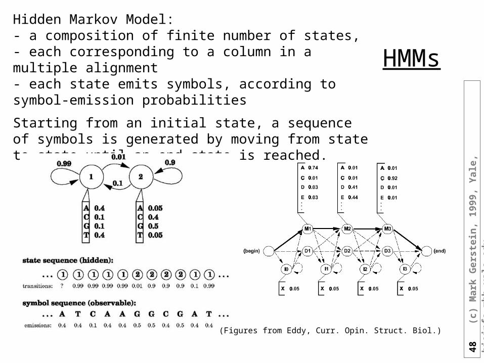
HMMs
Hidden Markov Model: - a composition of finite number of states, - each corresponding to a column in a multiple alignment - each state emits symbols, according to symbol-emission probabilities
Starting from an initial state, a sequence of symbols is generated by moving from state to state until an end state is reached.
(Figures from Eddy, Curr. Opin. Struct. Biol.)
49
(c)
Mar
k G
erst
ein
, 19
99,
Yal
e, b
ioin
fo.m
bb
.yal
e.ed
u
AB
CD
E0.5
0.5
0.1
0.3
0.2
0.8
0.4MM
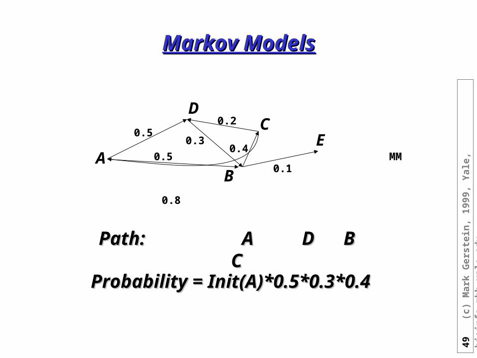
Markov ModelsMarkov Models
Path: Path: A D B CA D B C
Probability = Init(A)*0.5*0.3*0.4Probability = Init(A)*0.5*0.3*0.4
50
(c)
Mar
k G
erst
ein
, 19
99,
Yal
e, b
ioin
fo.m
bb
.yal
e.ed
u
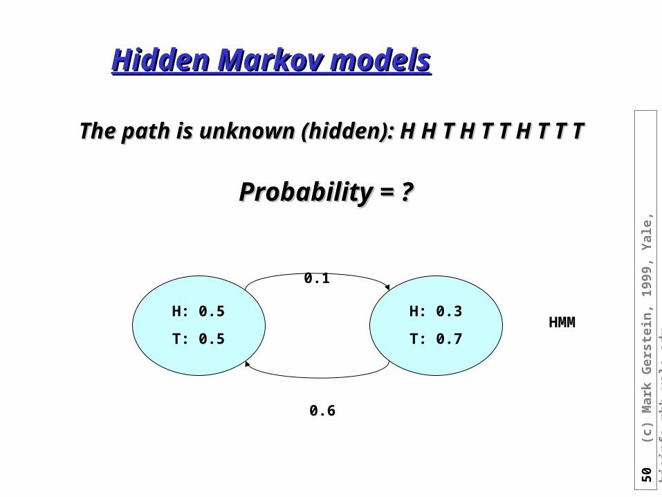
H: 0.5
T: 0.5
H: 0.3
T: 0.7
0.6
0.1
HMM
Hidden Markov modelsHidden Markov models
The path is unknown (hidden): H H T H T T H T T TThe path is unknown (hidden): H H T H T T H T T T
Probability = ?Probability = ?
51
(c)
Mar
k G
erst
ein
, 19
99,
Yal
e, b
ioin
fo.m
bb
.yal
e.ed
u
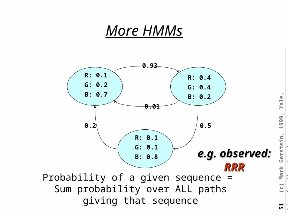
More HMMs
R: 0.1
G: 0.2
B: 0.7
R: 0.1
G: 0.1
B: 0.8
R: 0.4
G: 0.4
B: 0.2
0.93
0.01
0.50.2
Probability of a given sequence = Sum probability over ALL paths giving that sequence
e.g. observed: e.g. observed: RRRRRR
52
(c)
Mar
k G
erst
ein
, 19
99,
Yal
e, b
ioin
fo.m
bb
.yal
e.ed
u
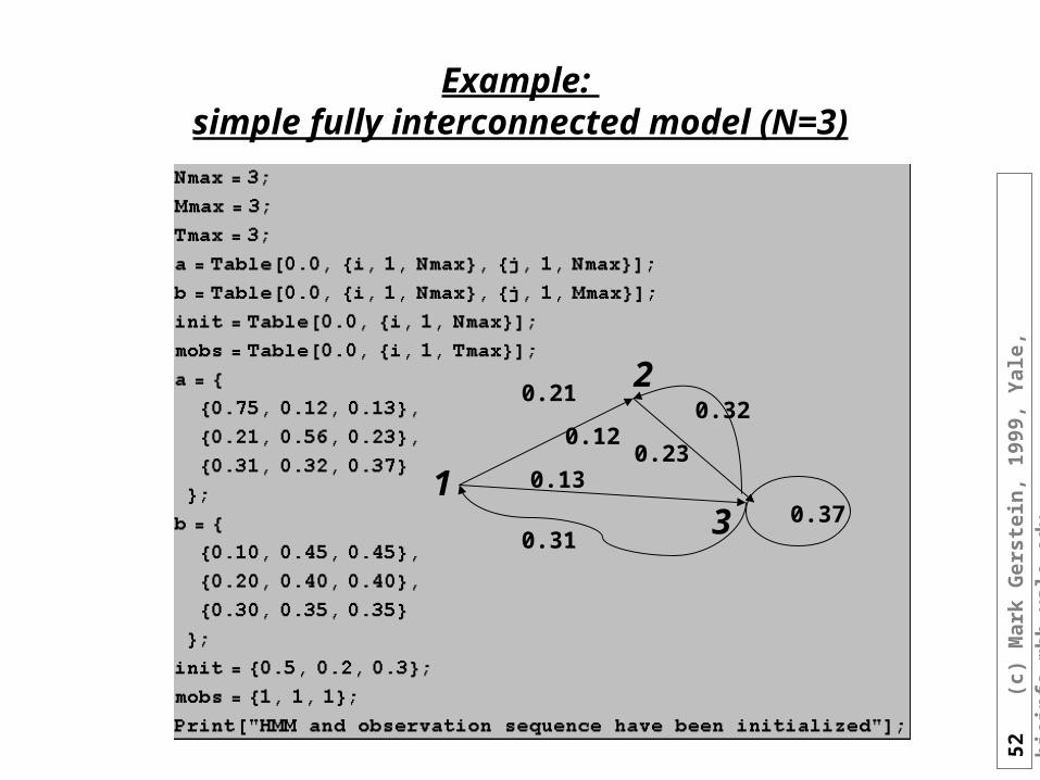
Example: simple fully interconnected model (N=3)
13
2
0.13
0.120.23
0.31
0.32
0.37
0.21
53
(c)
Mar
k G
erst
ein
, 19
99,
Yal
e, b
ioin
fo.m
bb
.yal
e.ed
u
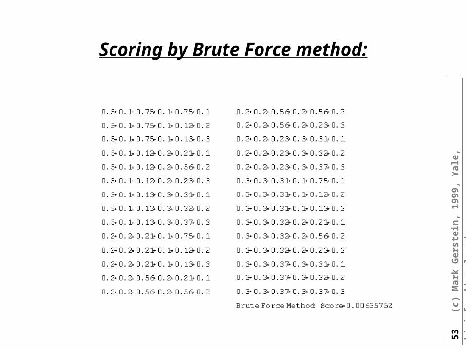
Scoring by Brute Force method:
54
(c)
Mar
k G
erst
ein
, 19
99,
Yal
e, b
ioin
fo.m
bb
.yal
e.ed
u
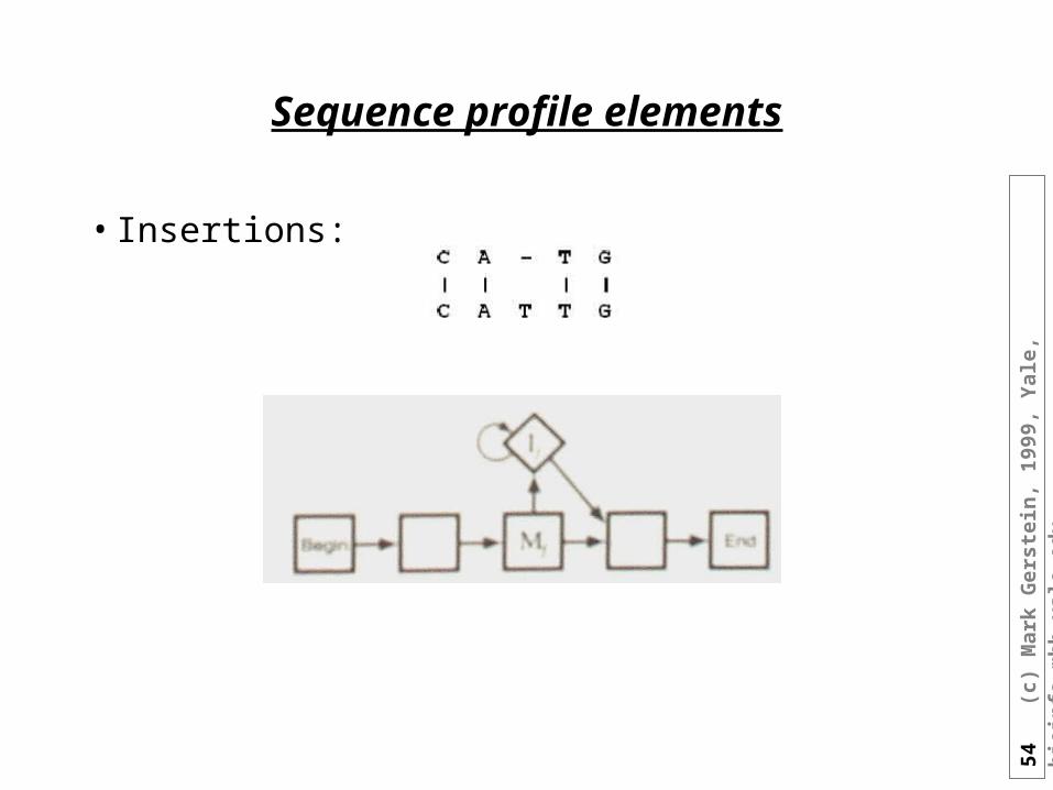
Sequence profile elements
• Insertions:
55
(c)
Mar
k G
erst
ein
, 19
99,
Yal
e, b
ioin
fo.m
bb
.yal
e.ed
u
Sequence profile elements
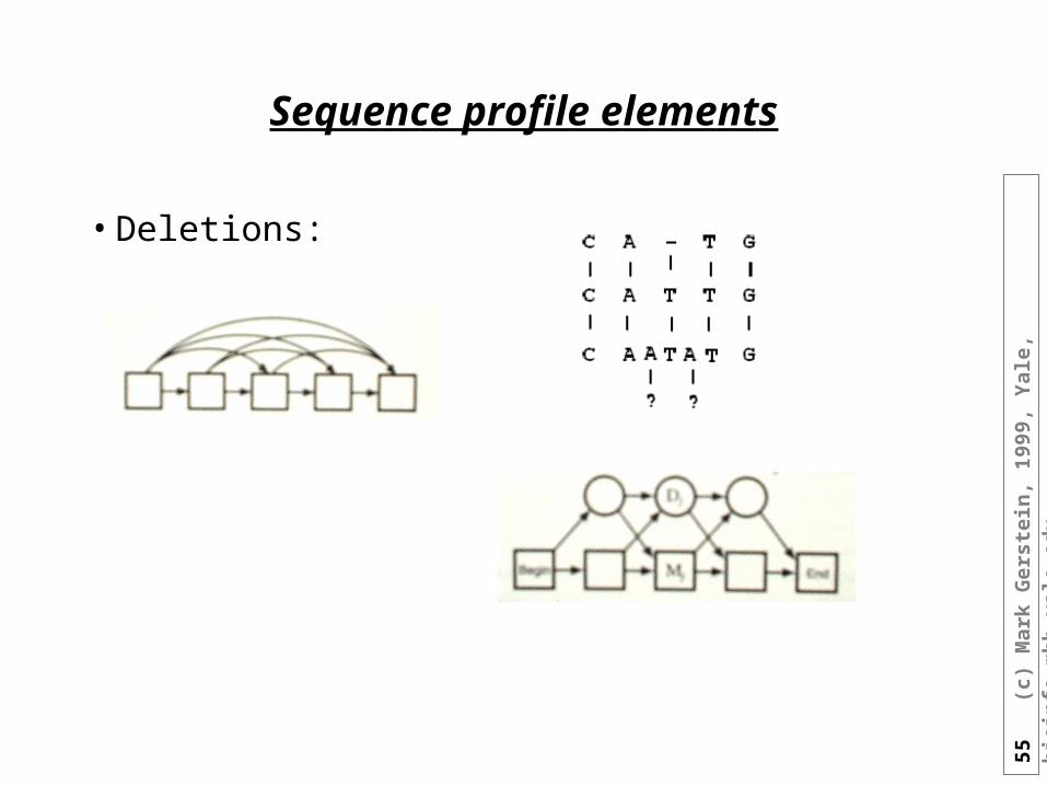
• Deletions:
56
(c)
Mar
k G
erst
ein
, 19
99,
Yal
e, b
ioin
fo.m
bb
.yal
e.ed
u
HMM sequence profiles
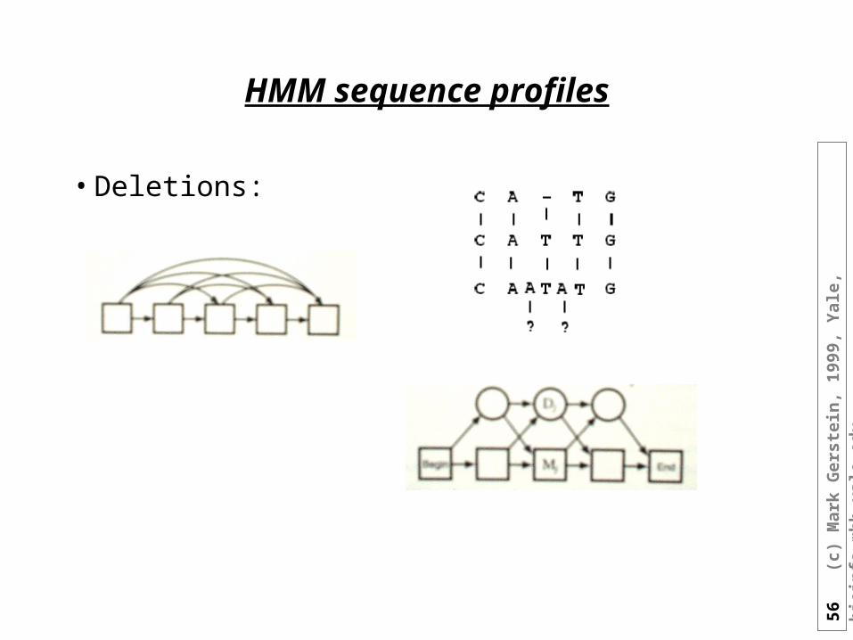
• Deletions:
57
(c)
Mar
k G
erst
ein
, 19
99,
Yal
e, b
ioin
fo.m
bb
.yal
e.ed
u
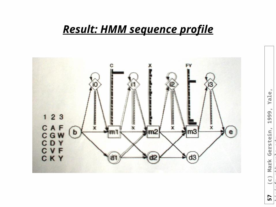
Result: HMM sequence profile
58
(c)
Mar
k G
erst
ein
, 19
99,
Yal
e, b
ioin
fo.m
bb
.yal
e.ed
u
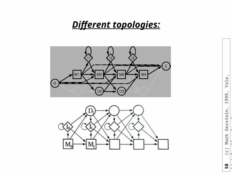
Different topologies:
59
(c)
Mar
k G
erst
ein
, 19
99,
Yal
e, b
ioin
fo.m
bb
.yal
e.ed
u
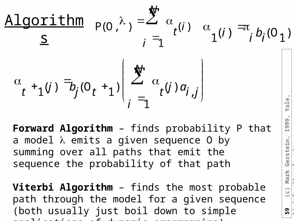
Algorithms ( )1 i
i ( )bi O1
( ) t 1 j ( )bj O t 1
i 1
N
( )t j a ,i j
( )P ,O i 1
N
( )t i
Forward Algorithm – finds probability P that a model emits a given sequence O by summing over all paths that emit the sequence the probability of that path
Viterbi Algorithm – finds the most probable path through the model for a given sequence(both usually just boil down to simple applications of dynamic programming)
60
(c)
Mar
k G
erst
ein
, 19
99,
Yal
e, b
ioin
fo.m
bb
.yal
e.ed
u
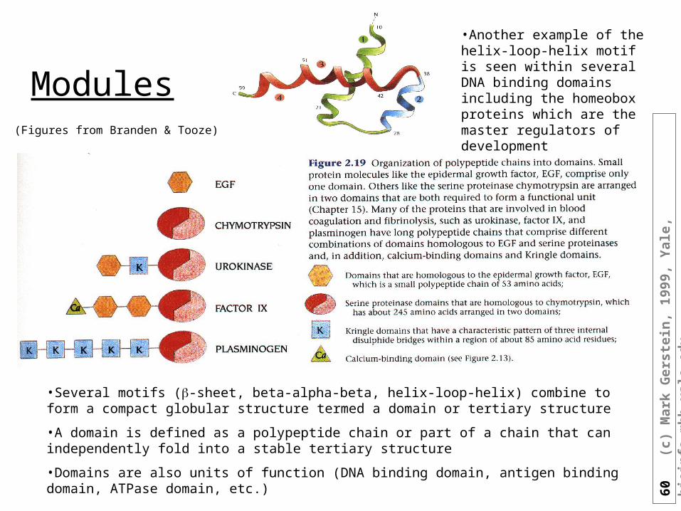
•Several motifs (-sheet, beta-alpha-beta, helix-loop-helix) combine to form a compact globular structure termed a domain or tertiary structure
•A domain is defined as a polypeptide chain or part of a chain that can independently fold into a stable tertiary structure
•Domains are also units of function (DNA binding domain, antigen binding domain, ATPase domain, etc.)
•Another example of the helix-loop-helix motif is seen within several DNA binding domains including the homeobox proteins which are the master regulators of development
Modules(Figures from Branden & Tooze)
61
(c)
Mar
k G
erst
ein
, 19
99,
Yal
e, b
ioin
fo.m
bb
.yal
e.ed
u
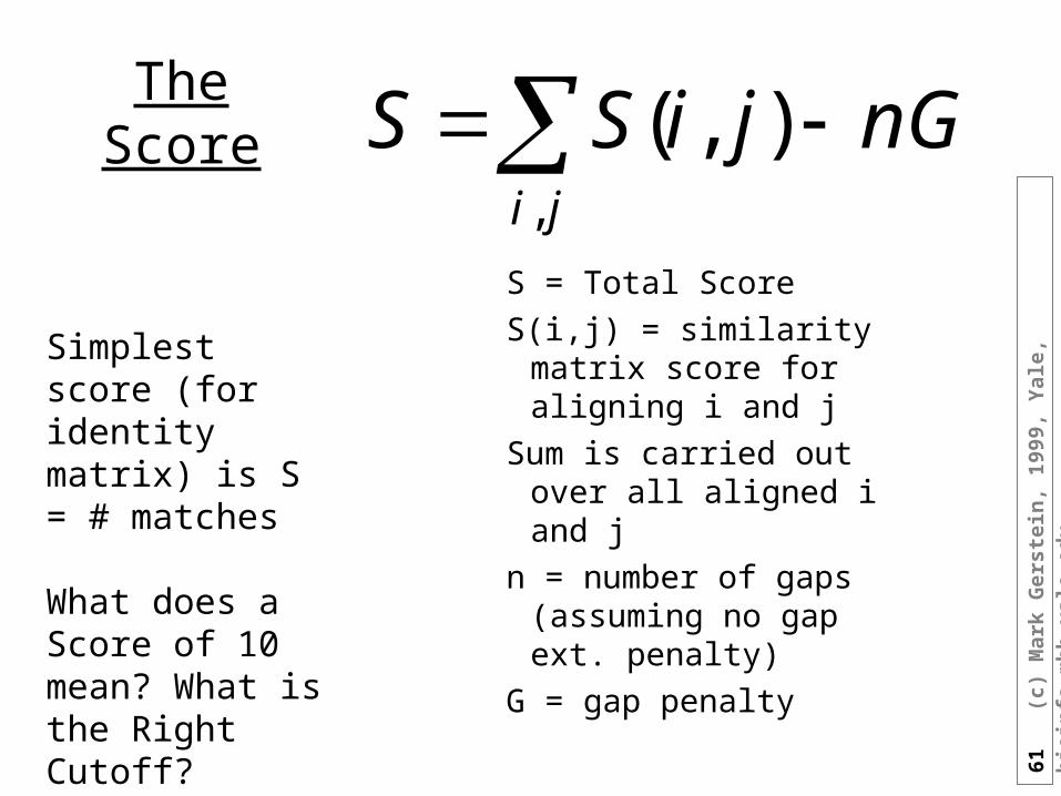
The Score
S = Total Score
S(i,j) = similarity matrix score for aligning i and j
Sum is carried out over all aligned i and j
n = number of gaps (assuming no gap ext. penalty)
G = gap penalty
nGjiSSji
,
),(
Simplest score (for identity matrix) is S = # matches
What does a Score of 10 mean? What is the Right Cutoff?
62
(c)
Mar
k G
erst
ein
, 19
99,
Yal
e, b
ioin
fo.m
bb
.yal
e.ed
u
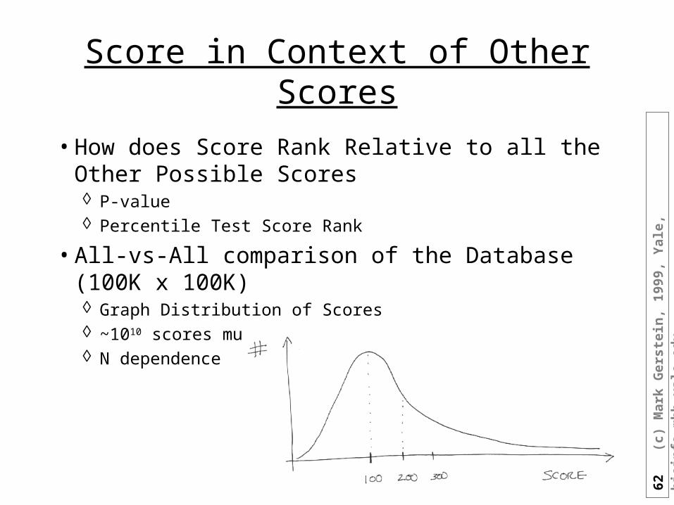
Score in Context of Other Scores
• How does Score Rank Relative to all the Other Possible Scores P-value Percentile Test Score Rank
• All-vs-All comparison of the Database (100K x 100K) Graph Distribution of Scores ~1010 scores much smaller number of true positives N dependence
63
(c)
Mar
k G
erst
ein
, 19
99,
Yal
e, b
ioin
fo.m
bb
.yal
e.ed
u
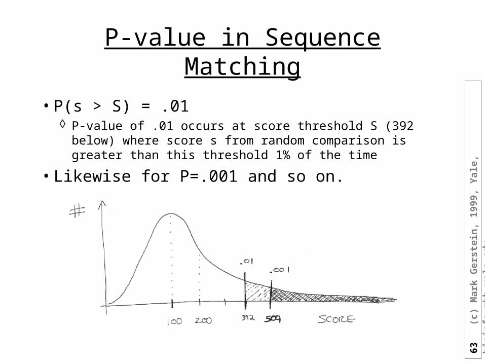
P-value in Sequence Matching
• P(s > S) = .01 P-value of .01 occurs at score threshold S (392 below) where score s
from random comparison is greater than this threshold 1% of the time
• Likewise for P=.001 and so on.
64
(c)
Mar
k G
erst
ein
, 19
99,
Yal
e, b
ioin
fo.m
bb
.yal
e.ed
u
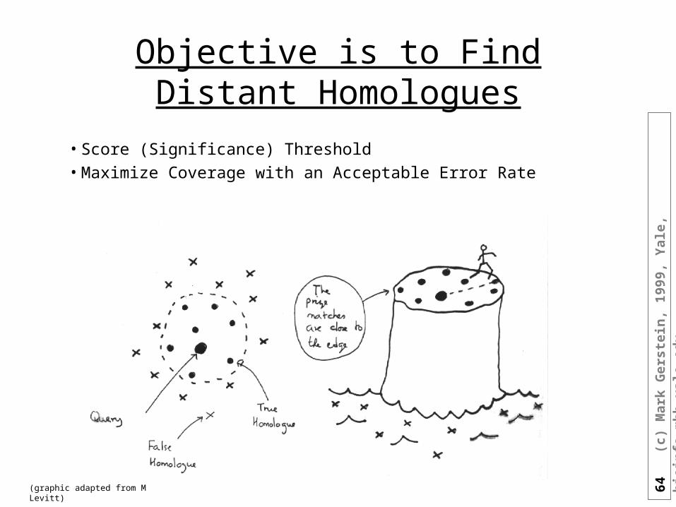
Objective is to Find Distant Homologues
• Score (Significance) Threshold
• Maximize Coverage with an Acceptable Error Rate
(graphic adapted from M Levitt)
65
(c)
Mar
k G
erst
ein
, 19
99,
Yal
e, b
ioin
fo.m
bb
.yal
e.ed
u
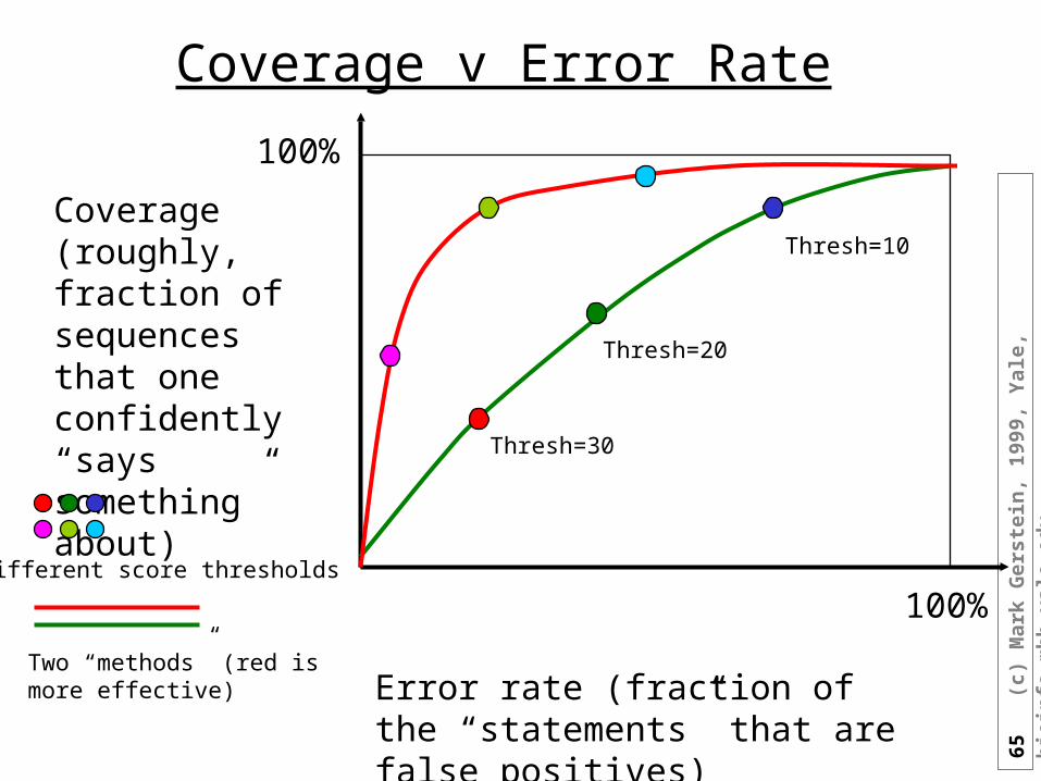
Coverage v Error Rate
Error rate (fraction of the “statements” that are false positives)
Coverage (roughly, fraction of sequences that one confidently “says something” about)
100%
100%Different score thresholds
Two “methods” (red is more effective)
Thresh=30
Thresh=20
Thresh=10
66
(c)
Mar
k G
erst
ein
, 19
99,
Yal
e, b
ioin
fo.m
bb
.yal
e.ed
u
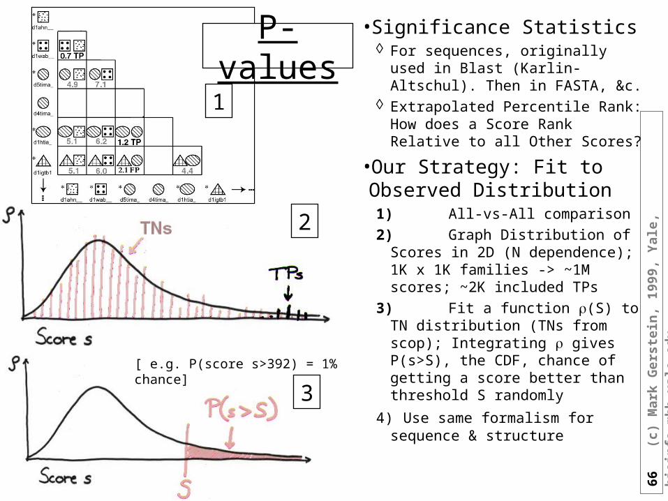
•Significance Statistics For sequences, originally used in
Blast (Karlin-Altschul). Then in FASTA, &c.
Extrapolated Percentile Rank: How does a Score Rank Relative to all Other Scores?
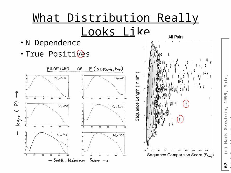
•Our Strategy: Fit to Observed Distribution1)All-vs-All comparison
2)Graph Distribution of Scores in 2D (N dependence); 1K x 1K families -> ~1M scores; ~2K included TPs
3)Fit a function (S) to TN distribution (TNs from scop); Integrating gives P(s>S), the CDF, chance of getting a score better than threshold S randomly
4) Use same formalism for sequence & structure
[ e.g. P(score s>392) = 1% chance]
1
2
3
P-values
67
(c)
Mar
k G
erst
ein
, 19
99,
Yal
e, b
ioin
fo.m
bb
.yal
e.ed
u
What Distribution Really Looks Like
• N Dependence• True Positives
68
(c)
Mar
k G
erst
ein
, 19
99,
Yal
e, b
ioin
fo.m
bb
.yal
e.ed
u
)exp(1)()( ZedzzZzP
zezz exp)(
zezz )(ln
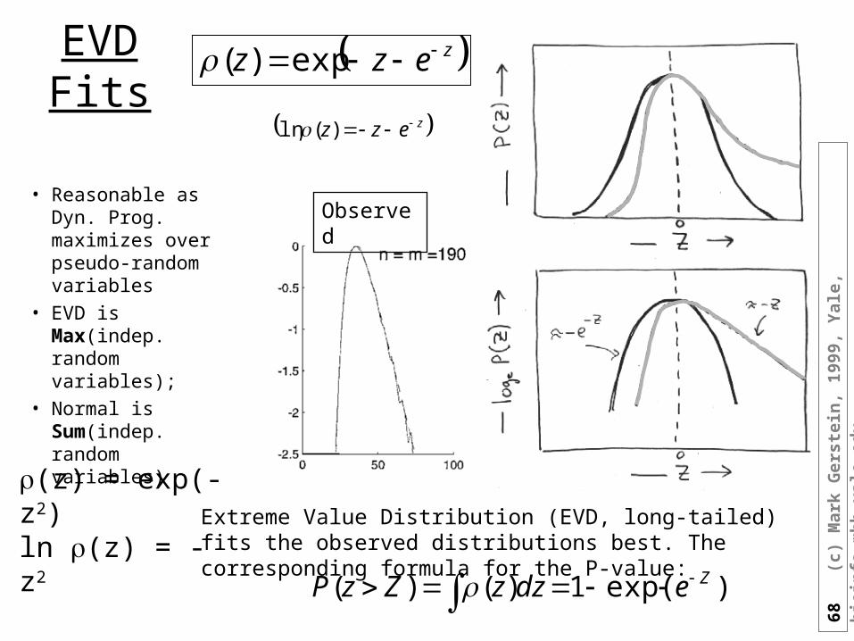
Extreme Value Distribution (EVD, long-tailed) fits the observed distributions best. The corresponding formula for the P-value:
EVD Fits
• Reasonable as Dyn. Prog. maximizes over pseudo-random variables
• EVD is Max(indep. random variables);
• Normal is Sum(indep. random variables)
Observed
(z) = exp(-z2) ln (z) = -z2
69
(c)
Mar
k G
erst
ein
, 19
99,
Yal
e, b
ioin
fo.m
bb
.yal
e.ed
u
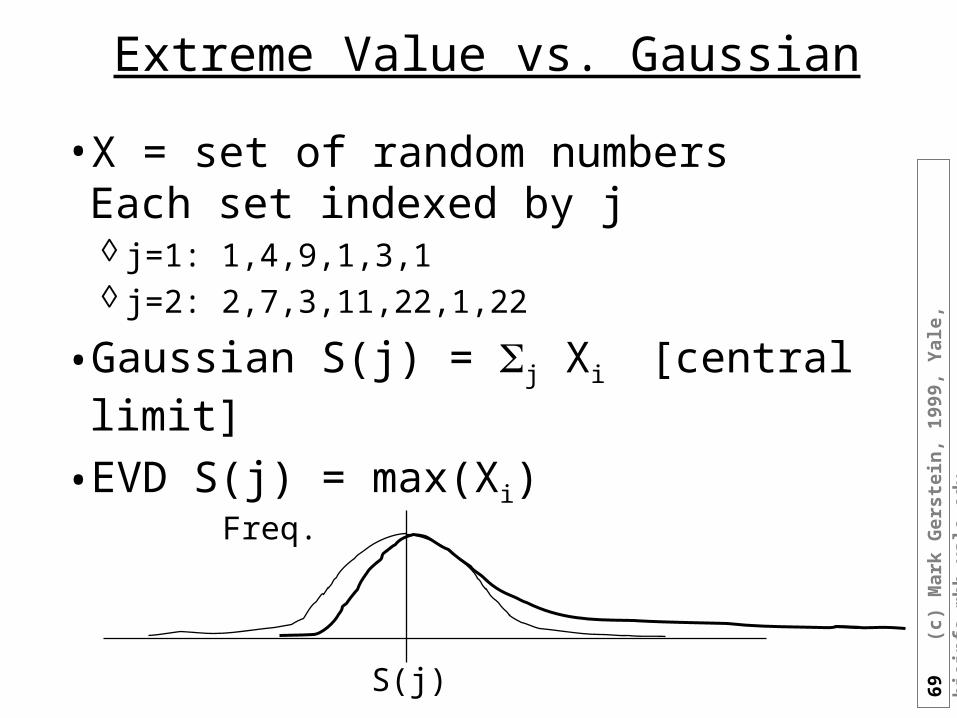
Extreme Value vs. Gaussian
• X = set of random numbers Each set indexed by j j=1: 1,4,9,1,3,1 j=2: 2,7,3,11,22,1,22
• Gaussian S(j) = j Xi [central limit]
• EVD S(j) = max(Xi)
S(j)
Freq.
70
(c)
Mar
k G
erst
ein
, 19
99,
Yal
e, b
ioin
fo.m
bb
.yal
e.ed
u
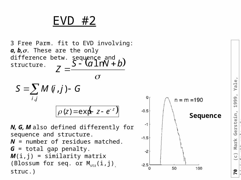
bNaSZ
ln
3 Free Parm. fit to EVD involving: a, b,. These are the only difference betw. sequence and structure.
EVD #2
N, G, M also defined differently for sequence and structure. N = number of residues matched.G = total gap penalty. M(i,j) = similarity matrix (Blossum for seq. or Mstr(i,j), struc.)
GjiMSji
,
),(
Sequence zezz exp)(

71
(c)
Mar
k G
erst
ein
, 19
99,
Yal
e, b
ioin
fo.m
bb
.yal
e.ed
u
End of Class 2
72
(c)
Mar
k G
erst
ein
, 19
99,
Yal
e, b
ioin
fo.m
bb
.yal
e.ed
u
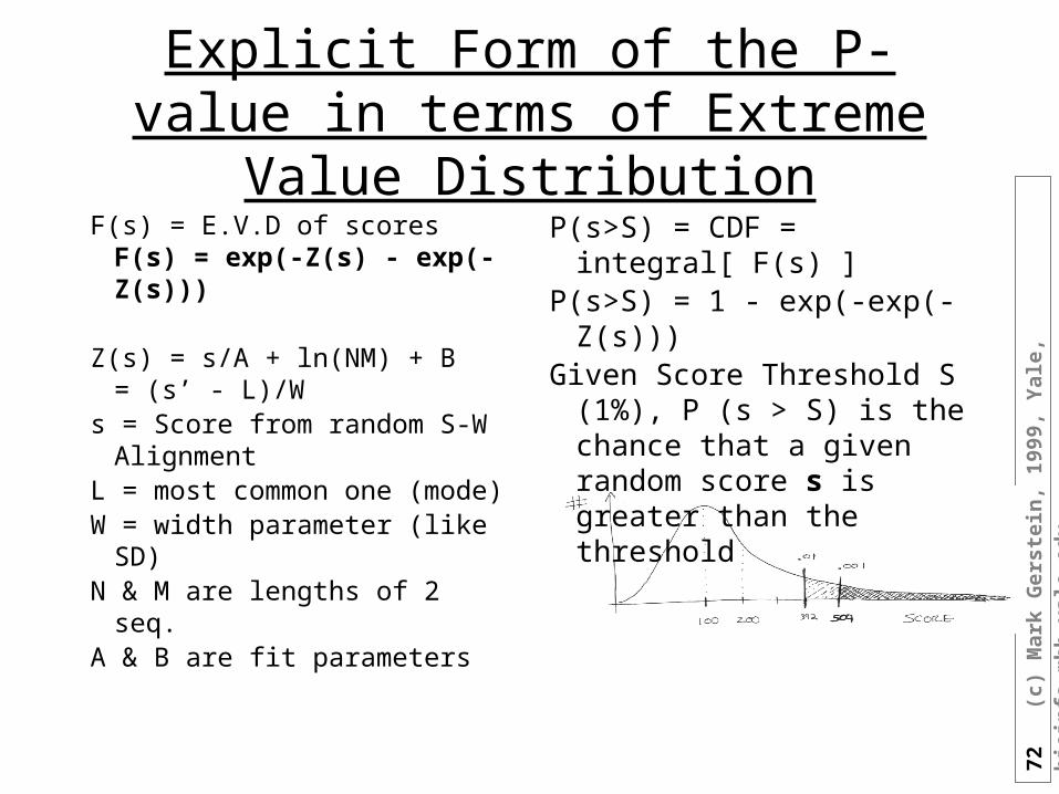
Explicit Form of the P-value in terms of Extreme Value Distribution
F(s) = E.V.D of scoresF(s) = exp(-Z(s) - exp(-Z(s)))
Z(s) = s/A + ln(NM) + B = (s’ - L)/W
s = Score from random S-W Alignment
L = most common one (mode)W = width parameter (like SD)N & M are lengths of 2 seq.A & B are fit parameters
P(s>S) = CDF = integral[ F(s) ] P(s>S) = 1 - exp(-exp(-Z(s)))Given Score Threshold S (1%),
P (s > S) is the chance that a given random score s is greater than the threshold
73
(c)
Mar
k G
erst
ein
, 19
99,
Yal
e, b
ioin
fo.m
bb
.yal
e.ed
u
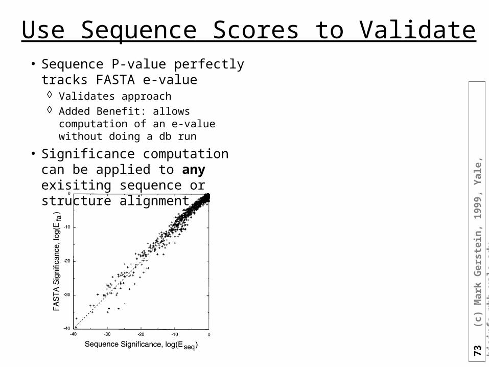
Use Sequence Scores to Validate• Sequence P-value perfectly tracks
FASTA e-value Validates approach Added Benefit: allows computation of
an e-value without doing a db run
• Significance computation can be applied to any exisiting sequence or structure alignment
74
(c)
Mar
k G
erst
ein
, 19
99,
Yal
e, b
ioin
fo.m
bb
.yal
e.ed
u
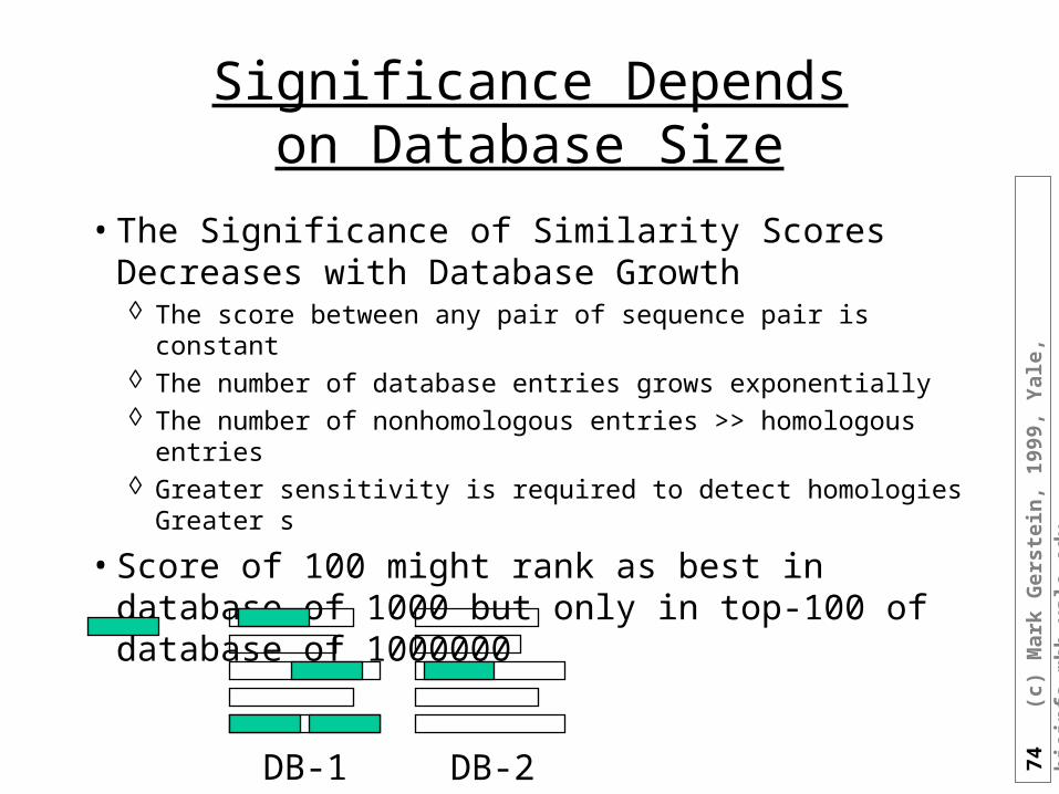
Significance Dependson Database Size
• The Significance of Similarity Scores Decreases with Database Growth The score between any pair of sequence pair is constant The number of database entries grows exponentially The number of nonhomologous entries >> homologous entries Greater sensitivity is required to detect homologies
Greater s
• Score of 100 might rank as best in database of 1000 but only in top-100 of database of 1000000
DB-1 DB-2
75
(c)
Mar
k G
erst
ein
, 19
99,
Yal
e, b
ioin
fo.m
bb
.yal
e.ed
u
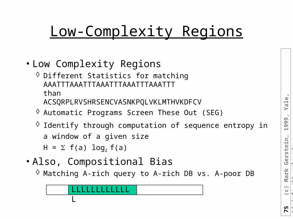
Low-Complexity Regions
• Low Complexity Regions Different Statistics for matching
AAATTTAAATTTAAATTTAAATTTAAATTTthanACSQRPLRVSHRSENCVASNKPQLVKLMTHVKDFCV
Automatic Programs Screen These Out (SEG)
Identify through computation of sequence entropy in a window of a
given size
H = f(a) log2 f(a)
• Also, Compositional Bias Matching A-rich query to A-rich DB vs. A-poor DB
LLLLLLLLLLLLL
76
(c)
Mar
k G
erst
ein
, 19
99,
Yal
e, b
ioin
fo.m
bb
.yal
e.ed
u
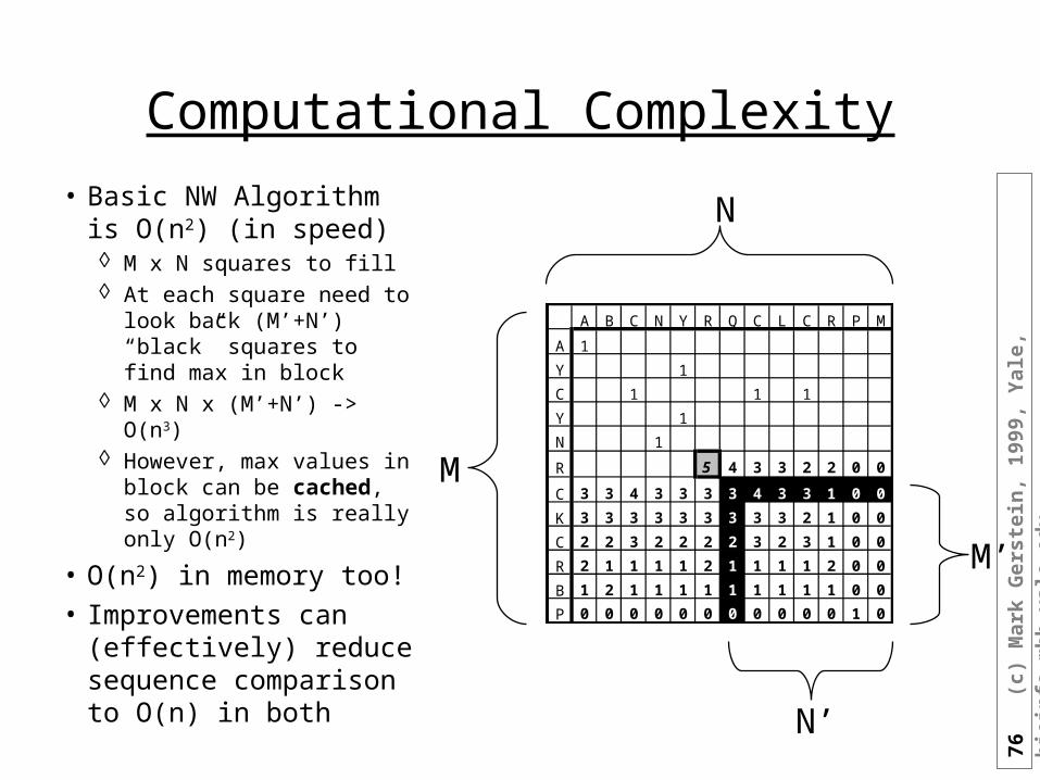
Computational Complexity
• Basic NW Algorithm is O(n2) (in speed) M x N squares to fill At each square need to
look back (M’+N’) “black” squares to find max in block
M x N x (M’+N’) -> O(n3) However, max values in
block can be cached, so algorithm is really only O(n2)
• O(n2) in memory too!• Improvements can
(effectively) reduce sequence comparison to O(n) in both
A B C N Y R Q C L C R P M
A 1
Y 1
C 1 1 1
Y 1
N 1
R 5 4 3 3 2 2 0 0
C 3 3 4 3 3 3 3 4 3 3 1 0 0
K 3 3 3 3 3 3 3 3 3 2 1 0 0
C 2 2 3 2 2 2 2 3 2 3 1 0 0
R 2 1 1 1 1 2 1 1 1 1 2 0 0
B 1 2 1 1 1 1 1 1 1 1 1 0 0
P 0 0 0 0 0 0 0 0 0 0 0 1 0
N
M
N’
M’
77
(c)
Mar
k G
erst
ein
, 19
99,
Yal
e, b
ioin
fo.m
bb
.yal
e.ed
u
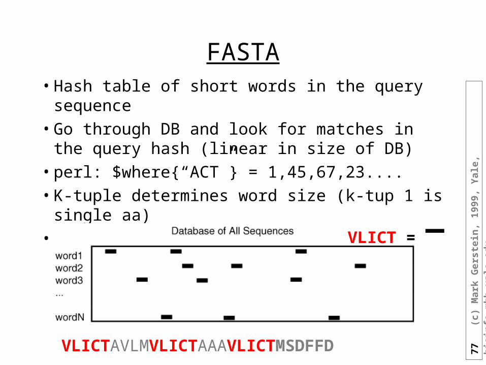
FASTA• Hash table of short words in the query sequence• Go through DB and look for matches in the query
hash (linear in size of DB)• perl: $where{“ACT”} = 1,45,67,23....• K-tuple determines word size (k-tup 1 is single aa)• by Bill Pearson
VLICTAVLMVLICTAAAVLICTMSDFFD
VLICT = _
78
(c)
Mar
k G
erst
ein
, 19
99,
Yal
e, b
ioin
fo.m
bb
.yal
e.ed
u
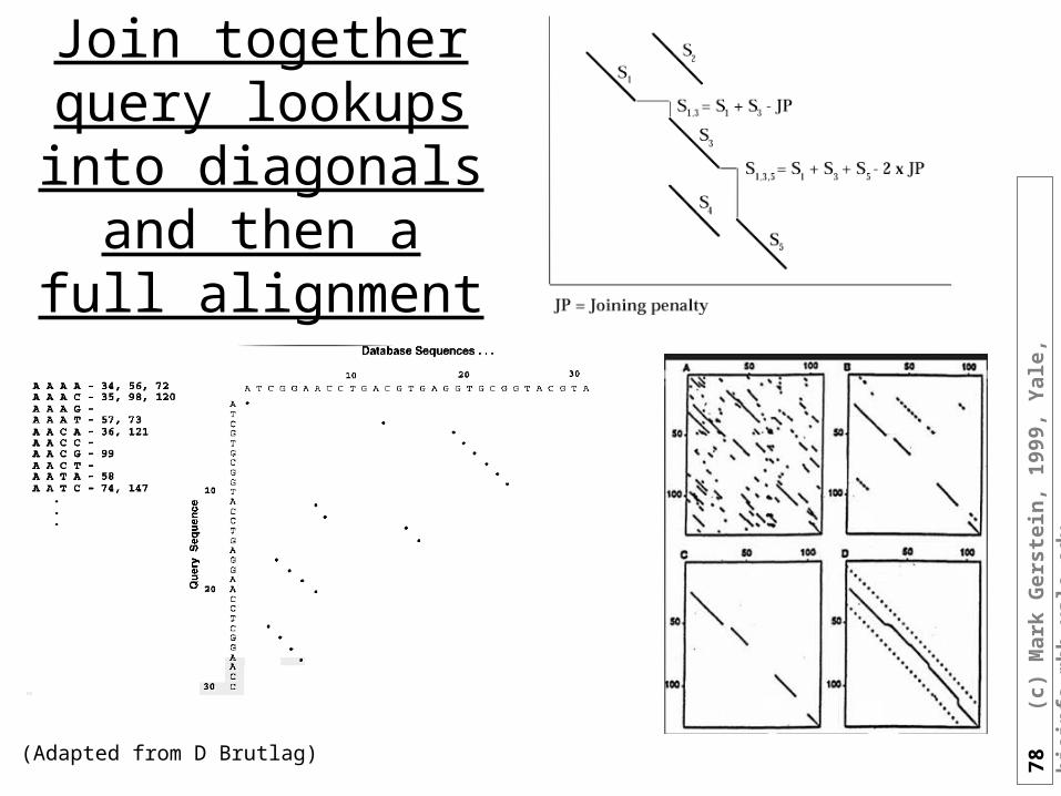
Join together query lookups into
diagonals and then a full alignment
(Adapted from D Brutlag)
79
(c)
Mar
k G
erst
ein
, 19
99,
Yal
e, b
ioin
fo.m
bb
.yal
e.ed
u
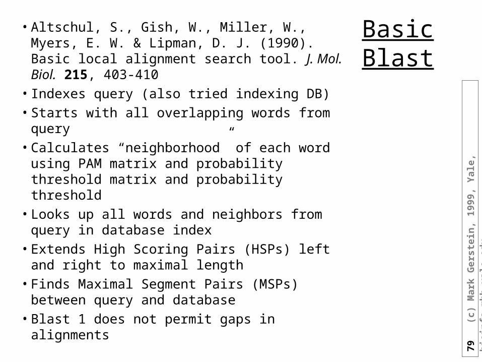
Basic Blast
• Altschul, S., Gish, W., Miller, W., Myers, E. W. & Lipman, D. J. (1990). Basic local alignment search tool. J. Mol. Biol. 215, 403-410
• Indexes query (also tried indexing DB)• Starts with all overlapping words from query• Calculates “neighborhood” of each word using
PAM matrix and probability threshold matrix and probability threshold
• Looks up all words and neighbors from query in database index
• Extends High Scoring Pairs (HSPs) left and right to maximal length
• Finds Maximal Segment Pairs (MSPs) between query and database
• Blast 1 does not permit gaps in alignments
80
(c)
Mar
k G
erst
ein
, 19
99,
Yal
e, b
ioin
fo.m
bb
.yal
e.ed
u
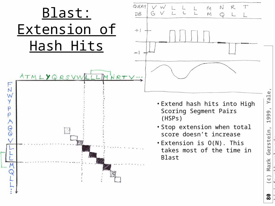
Blast: Extension of Hash Hits
• Extend hash hits into High Scoring Segment Pairs (HSPs)
• Stop extension when total score doesn’t increase
• Extension is O(N). This takes most of the time in Blast
81
(c)
Mar
k G
erst
ein
, 19
99,
Yal
e, b
ioin
fo.m
bb
.yal
e.ed
u
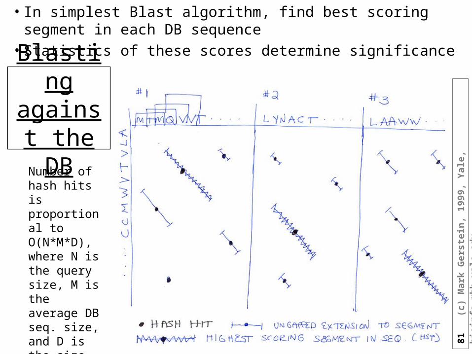
Blasting against the DB
• In simplest Blast algorithm, find best scoring segment in each DB sequence
• Statistics of these scores determine significance
Number of hash hits is proportional to O(N*M*D), where N is the query size, M is the average DB seq. size, and D is the size of the DB
82
(c)
Mar
k G
erst
ein
, 19
99,
Yal
e, b
ioin
fo.m
bb
.yal
e.ed
u
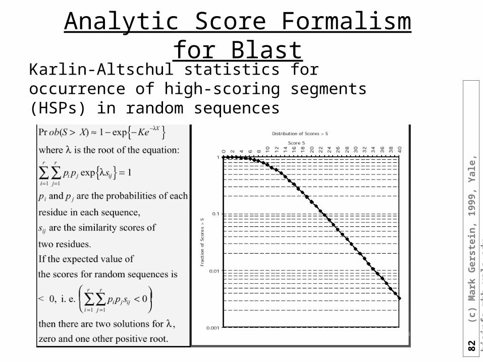
Analytic Score Formalism for BlastKarlin-Altschul statistics for occurrence of high-scoring segments (HSPs) in random sequences
83
(c)
Mar
k G
erst
ein
, 19
99,
Yal
e, b
ioin
fo.m
bb
.yal
e.ed
u
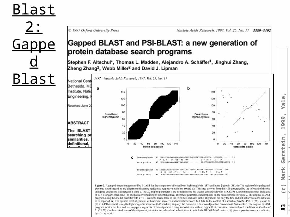
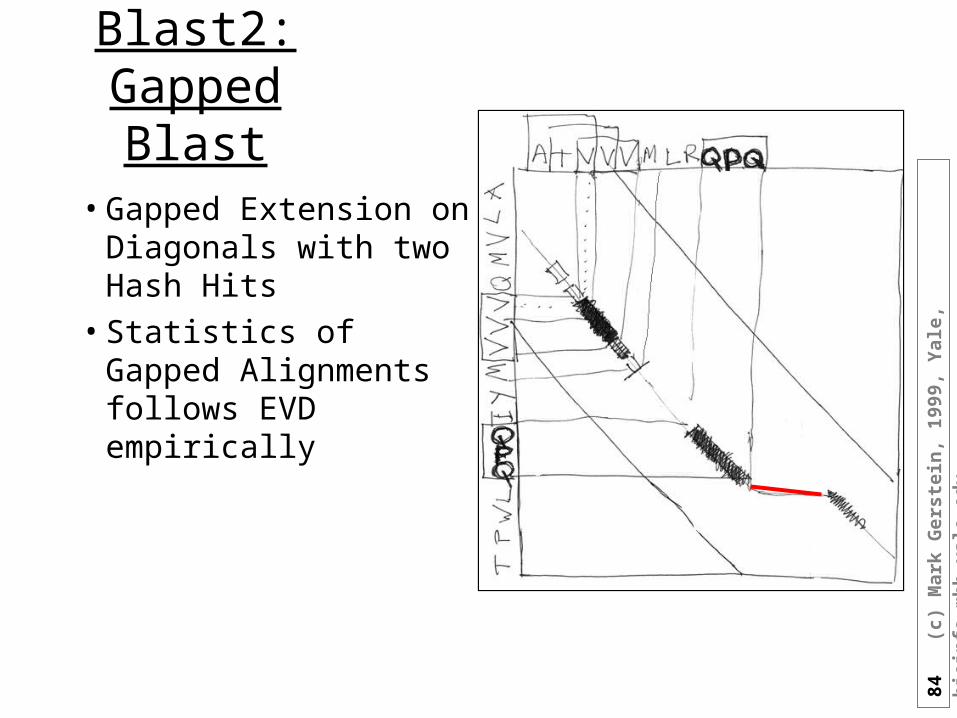
Blast2: Gapped
Blast
84
(c)
Mar
k G
erst
ein
, 19
99,
Yal
e, b
ioin
fo.m
bb
.yal
e.ed
u
Blast2: Gapped Blast
• Gapped Extension on Diagonals with two Hash Hits
• Statistics of Gapped Alignments follows EVD empirically
85
(c)
Mar
k G
erst
ein
, 19
99,
Yal
e, b
ioin
fo.m
bb
.yal
e.ed
u
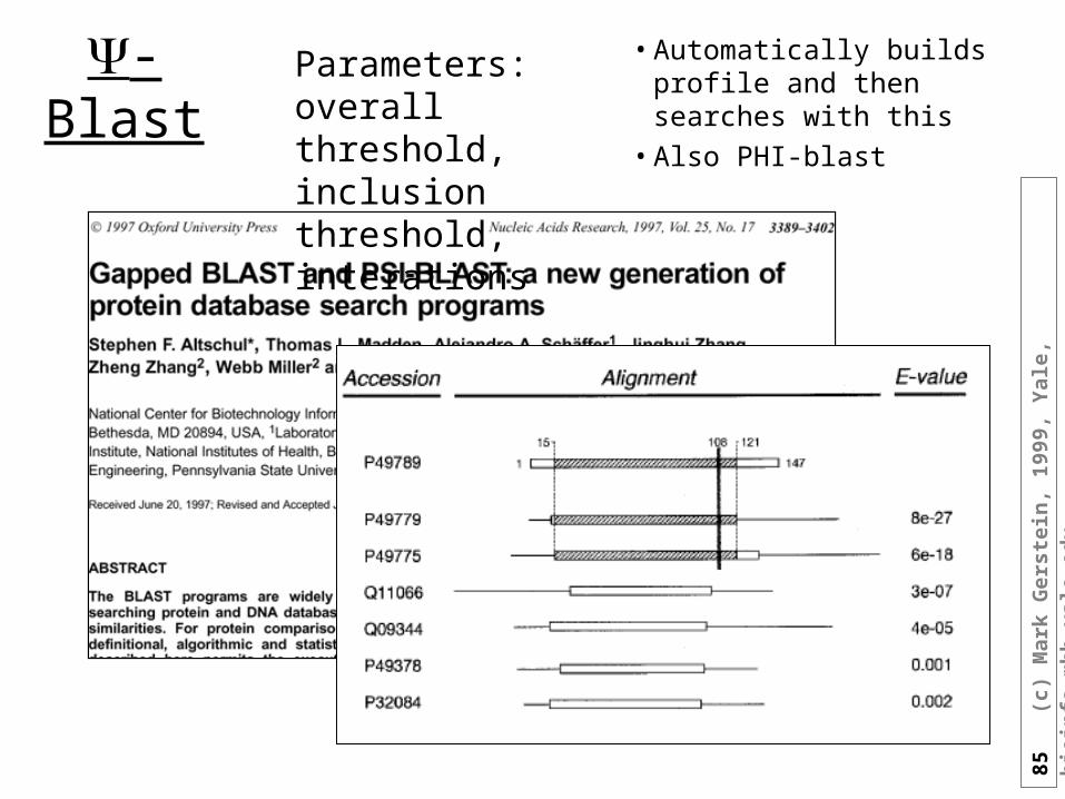
-Blast• Automatically builds profile
and then searches with this• Also PHI-blast
Parameters: overall threshold, inclusion threshold, interations
86
(c)
Mar
k G
erst
ein
, 19
99,
Yal
e, b
ioin
fo.m
bb
.yal
e.ed
u
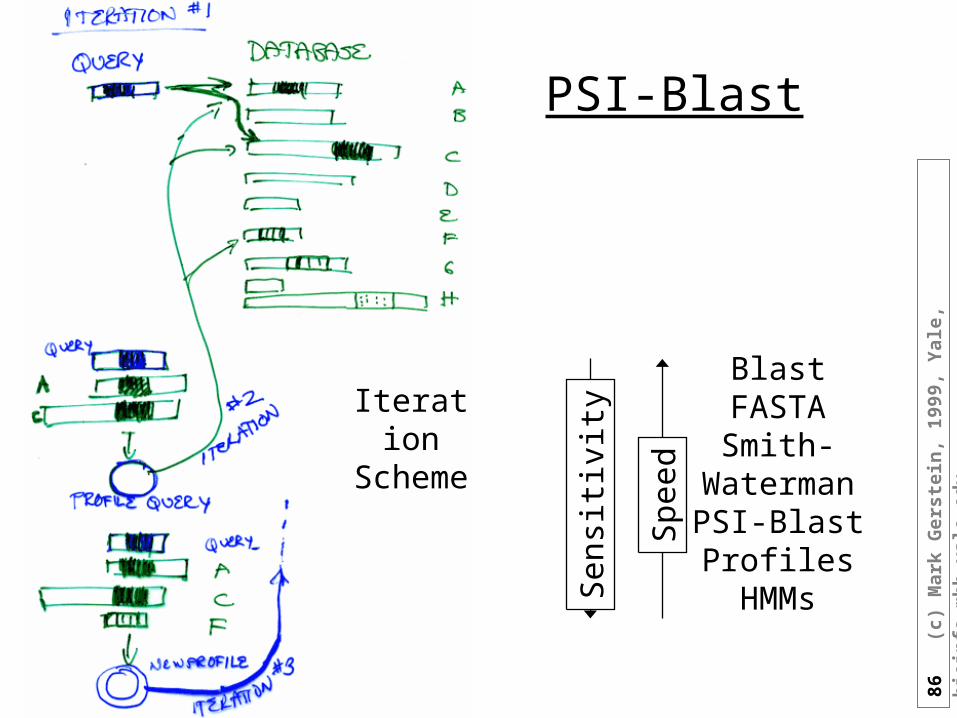
PSI-Blast
Iteration Scheme
BlastFASTASmith-
WatermanPSI-BlastProfilesHMMs
Spe
ed
Sen
sitiv
ity
87
(c)
Mar
k G
erst
ein
, 19
99,
Yal
e, b
ioin
fo.m
bb
.yal
e.ed
u
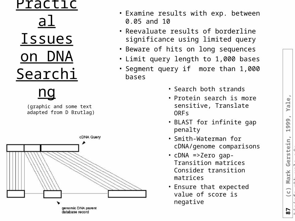
Practical Issues on
DNA Searching
• Examine results with exp. between 0.05 and 10
• Reevaluate results of borderline significance using limited query
• Beware of hits on long sequences
• Limit query length to 1,000 bases
• Segment query if more than 1,000 bases
• Search both strands • Protein search is more
sensitive, Translate ORFs• BLAST for infinite gap
penalty• Smith-Waterman for
cDNA/genome comparisons
• cDNA =>Zero gap-Transition matrices Consider transition matrices
• Ensure that expected value of score is negative
(graphic and some text adapted from D Brutlag)
88
(c)
Mar
k G
erst
ein
, 19
99,
Yal
e, b
ioin
fo.m
bb
.yal
e.ed
u
General Protein Search Principles
• Choose between local or global search algorithms
• Use most sensitive search algorithm available
• Original BLAST for no gaps• Smith-Waterman for most
sensitivity• FASTA with k-tuple 1 is a
good compromise• Gapped BLAST for well
delimited regions• PSI-BLAST for families• Initially BLOSUM62 and
default gap penalties
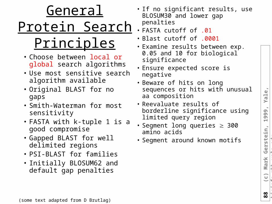
• If no significant results, use BLOSUM30 and lower gap penalties
• FASTA cutoff of .01• Blast cutoff of .0001• Examine results between exp. 0.05
and 10 for biological significance• Ensure expected score is negative• Beware of hits on long sequences or
hits with unusual aa composition• Reevaluate results of borderline
significance using limited query region
• Segment long queries 300 amino acids
• Segment around known motifs
(some text adapted from D Brutlag)
89
(c)
Mar
k G
erst
ein
, 19
99,
Yal
e, b
ioin
fo.m
bb
.yal
e.ed
u
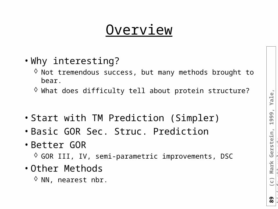
Overview
• Why interesting? Not tremendous success, but many methods brought to bear. What does difficulty tell about protein structure?
• Start with TM Prediction (Simpler)• Basic GOR Sec. Struc. Prediction• Better GOR
GOR III, IV, semi-parametric improvements, DSC
• Other Methods NN, nearest nbr.
90
(c)
Mar
k G
erst
ein
, 19
99,
Yal
e, b
ioin
fo.m
bb
.yal
e.ed
u
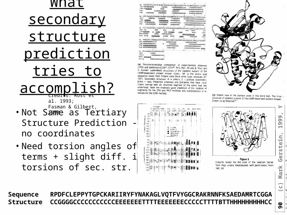
What secondary structure
prediction tries to accomplish?
• Not Same as Tertiary Structure Prediction -- no coordinates
• Need torsion angles of terms + slight diff. in torsions of sec. str.
Credits: Rost et al. 1993; Fasman & Gilbert, 1990
Sequence RPDFCLEPPYTGPCKARIIRYFYNAKAGLVQTFVYGGCRAKRNNFKSAEDAMRTCGGAStructure CCGGGGCCCCCCCCCCCEEEEEEETTTTEEEEEEECCCCCTTTTBTTHHHHHHHHHCC
91
(c)
Mar
k G
erst
ein
, 19
99,
Yal
e, b
ioin
fo.m
bb
.yal
e.ed
u
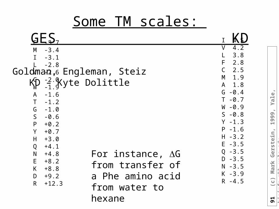
Some TM scales: GES KD I 4.5
V 4.2L 3.8F 2.8C 2.5M 1.9A 1.8G -0.4T -0.7W -0.9S -0.8Y -1.3P -1.6H -3.2E -3.5Q -3.5D -3.5N -3.5 K -3.9R -4.5
F -3.7M -3.4I -3.1L -2.8V -2.6C -2.0W -1.9A -1.6T -1.2G -1.0S -0.6P +0.2Y +0.7H +3.0Q +4.1N +4.8E +8.2K +8.8D +9.2R +12.3
For instance, G from transfer of a Phe amino acid from water to hexane
Goldman, Engleman, SteizKD – Kyte Dolittle
92
(c)
Mar
k G
erst
ein
, 19
99,
Yal
e, b
ioin
fo.m
bb
.yal
e.ed
u
How to use GES to predict proteins
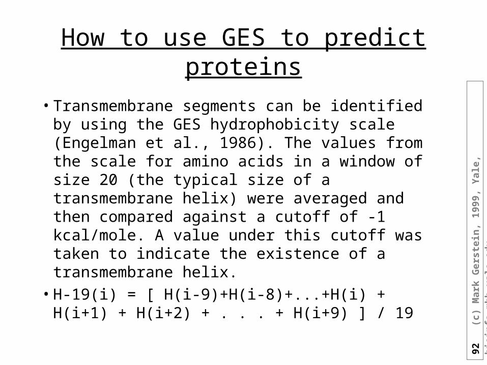
• Transmembrane segments can be identified by using the GES hydrophobicity scale (Engelman et al., 1986). The values from the scale for amino acids in a window of size 20 (the typical size of a transmembrane helix) were averaged and then compared against a cutoff of -1 kcal/mole. A value under this cutoff was taken to indicate the existence of a transmembrane helix.
• H-19(i) = [ H(i-9)+H(i-8)+...+H(i) + H(i+1) + H(i+2) + . . . + H(i+9) ] / 19
93
(c)
Mar
k G
erst
ein
, 19
99,
Yal
e, b
ioin
fo.m
bb
.yal
e.ed
u
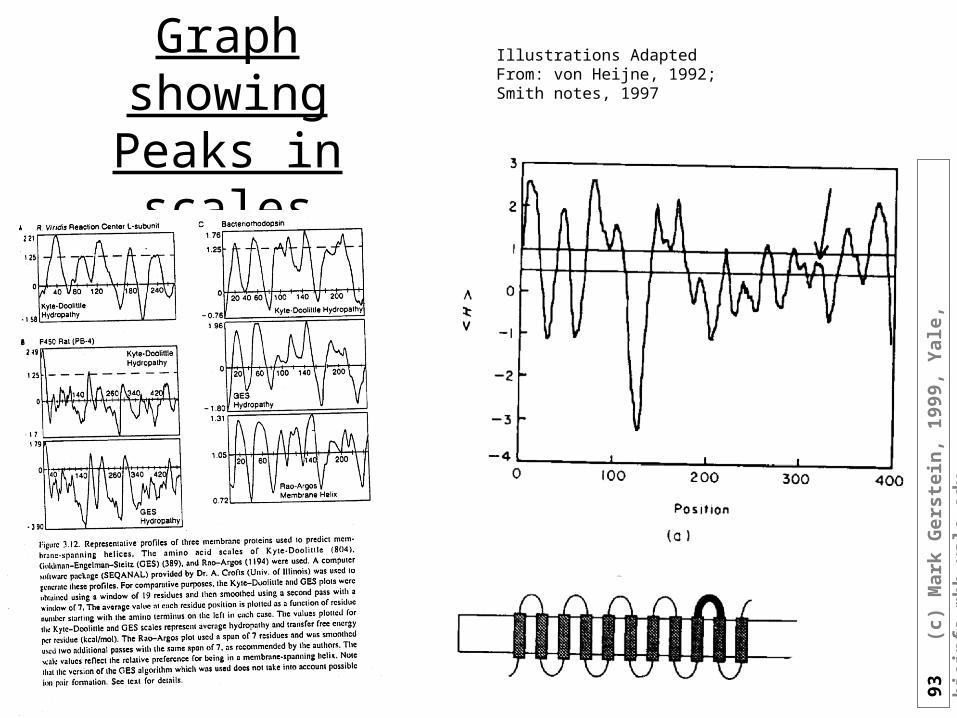
Graph showing Peaks in scales
Illustrations Adapted From: von Heijne, 1992; Smith notes, 1997
94
(c)
Mar
k G
erst
ein
, 19
99,
Yal
e, b
ioin
fo.m
bb
.yal
e.ed
u
Removing Signal sequences
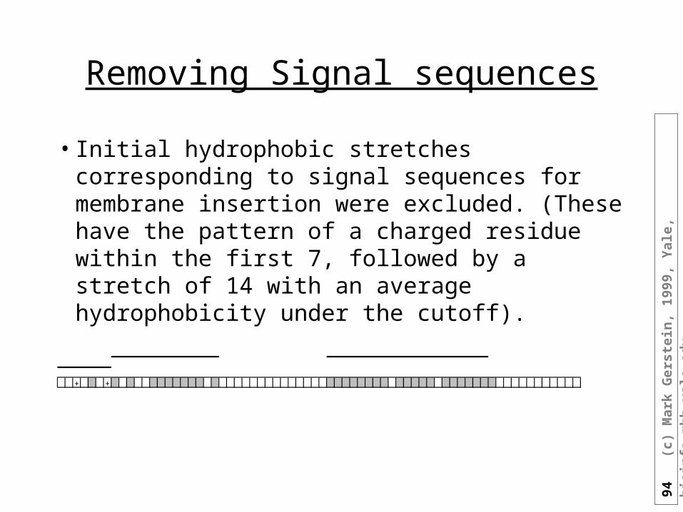
• Initial hydrophobic stretches corresponding to signal sequences for membrane insertion were excluded. (These have the pattern of a charged residue within the first 7, followed by a stretch of 14 with an average hydrophobicity under the cutoff).
+ +
95
(c)
Mar
k G
erst
ein
, 19
99,
Yal
e, b
ioin
fo.m
bb
.yal
e.ed
u
Ex. P(i,) probability that residue i has secondary structure
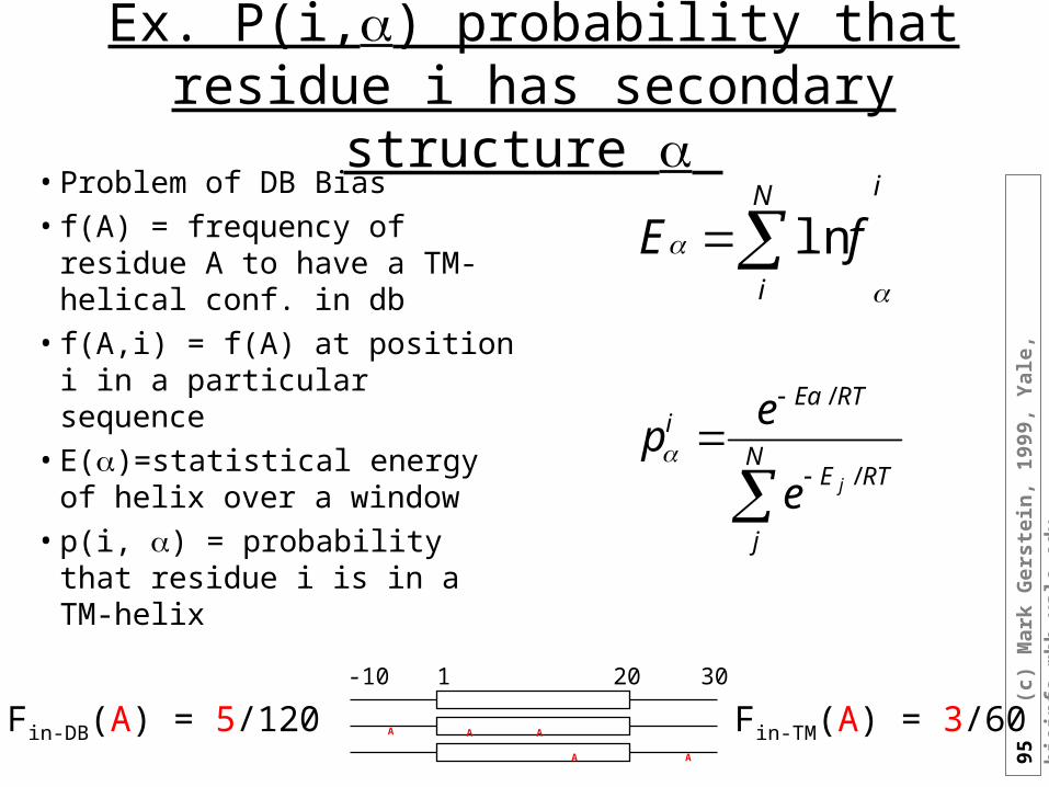
• Problem of DB Bias• f(A) = frequency of residue A
to have a TM-helical conf. in db
• f(A,i) = f(A) at position i in a particular sequence
• E()=statistical energy of helix over a window
• p(i, ) = probability that residue i is in a TM-helix
N
j
RTE
RTEai
je
ep
/
/
iN
i
fE
ln
1 20
A A
A
Fin-TM(A) = 3/60A
A
-10 30
Fin-DB(A) = 5/120

96
(c)
Mar
k G
erst
ein
, 19
99,
Yal
e, b
ioin
fo.m
bb
.yal
e.ed
u
End of Class 3
97
(c)
Mar
k G
erst
ein
, 19
99,
Yal
e, b
ioin
fo.m
bb
.yal
e.ed
u
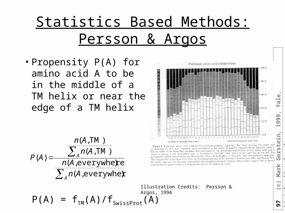
Statistics Based Methods:Persson & Argos
• Propensity P(A) for amino acid A to be in the middle of a TM helix or near the edge of a TM helix
A
A
AnAn
AnAn
AP
)everywhere,()everywhere,(
)TM,()TM,(
)(
Illustration Credits: Persson & Argos, 1994
P(A) = fTM(A)/fSwissProt(A)
98
(c)
Mar
k G
erst
ein
, 19
99,
Yal
e, b
ioin
fo.m
bb
.yal
e.ed
u
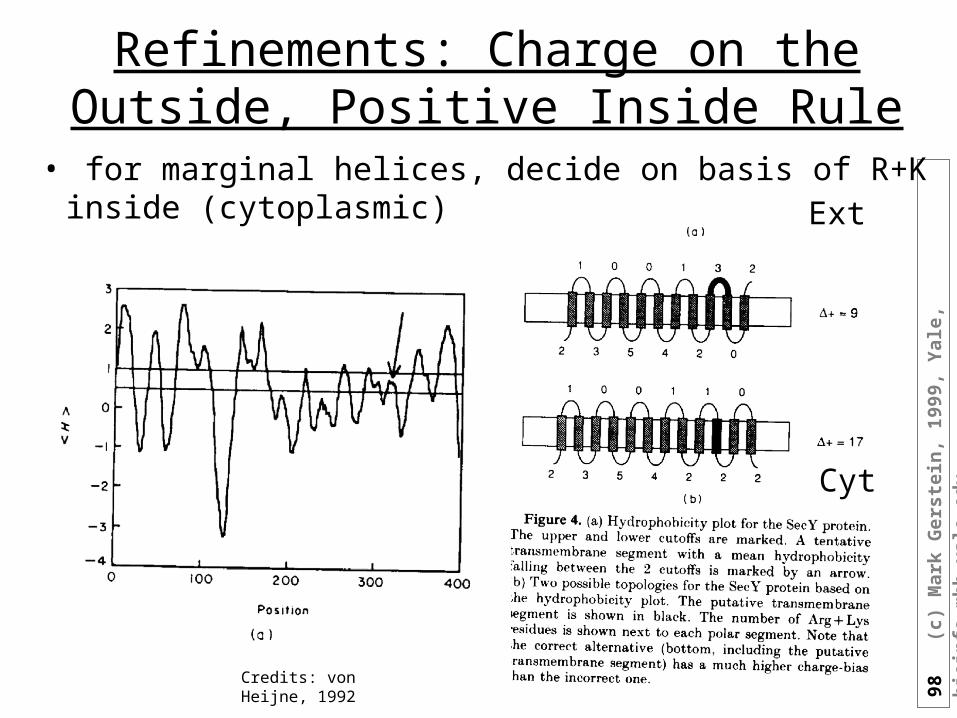
Refinements: Charge on the Outside, Positive Inside Rule
• for marginal helices, decide on basis of R+K inside (cytoplasmic)
Credits: von Heijne, 1992
Ext
Cyt
99
(c)
Mar
k G
erst
ein
, 19
99,
Yal
e, b
ioin
fo.m
bb
.yal
e.ed
u
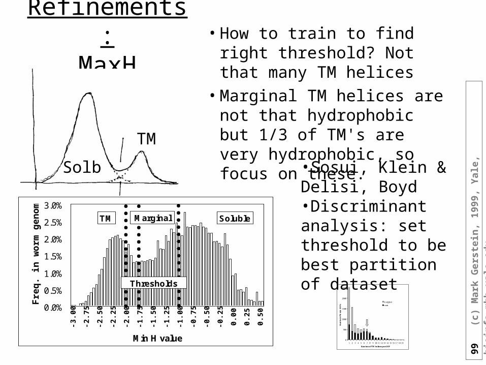
Refinements:MaxH
• How to train to find right threshold? Not that many TM helices
• Marginal TM helices are not that hydrophobic but 1/3 of TM's are very hydrophobic, so focus on these.
0.0%
0.5%
1.0%
1.5%
2.0%
2.5%
3.0%
-3.0
0
-2.7
5
-2.5
0
-2.2
5
-2.0
0
-1.7
5
-1.5
0
-1.2
5
-1.0
0
-0.7
5
-0.5
0
-0.2
5
0.0
0
0.2
5
0.5
0
Min H value
Fre
q.
in w
orm
gen
om
e
TM Marginal
Thresholds
Soluble
0
500
1000
1500
2000
2500
1 2 3 4 5 6 7 8 9 10 11 12 13 14 15 16 17 18 19
Number of TM helices per ORF
Nu
mb
er
of
Wo
rm O
RF
s
marginal
sure
•Sosui, Klein & Delisi, Boyd•Discriminant analysis: set threshold to be best partition of dataset
Solb
TM
100
(
c) M
ark
Ger
stei
n,
1999
, Y
ale,
bio
info
.mb
b.y
ale.
edu
GOR: Simplifications
• For independent events just add up the information
• I(Sj ; R1, R2, R3,...Rlast) = Information that first through last residue of protein has on the conformation of residue j (Sj) Could get this just from sequence sim. or if same struc. in DB
(homology best way to predict sec. struc.!)
• Simplify using a 17 residue window: I(Sj=H ; R[j-8], R[j-7], ...., R[j], .... R[j+8])
• Difference of information for residue to be in helix relative to not: I(dSj;y) = I(Sj=H;y)-I(Sj=~H;y) odds ratio: I(dSj;y)= ln P(Sj;y)/P(~Sj;y) I determined by observing counts in the DB, essentially a lod value
101
(
c) M
ark
Ger
stei
n,
1999
, Y
ale,
bio
info
.mb
b.y
ale.
edu
Basic GOR
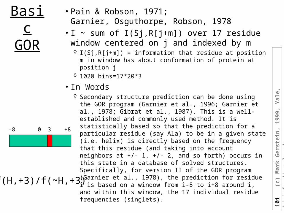
• Pain & Robson, 1971; Garnier, Osguthorpe, Robson, 1978
• I ~ sum of I(Sj,R[j+m]) over 17 residue window centered on j and indexed by m I(Sj,R[j+m]) = information that residue at position m in
window has about conformation of protein at position j 1020 bins=17*20*3
• In Words Secondary structure prediction can be done using the
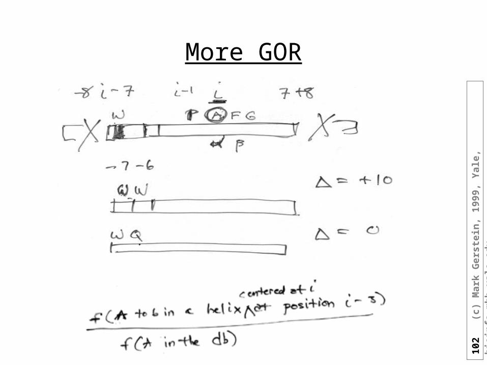
GOR program (Garnier et al., 1996; Garnier et al., 1978; Gibrat et al., 1987). This is a well-established and commonly used method. It is statistically based so that the prediction for a particular residue (say Ala) to be in a given state (i.e. helix) is directly based on the frequency that this residue (and taking into account neighbors at +/- 1, +/- 2, and so forth) occurs in this state in a database of solved structures. Specifically, for version II of the GOR program (Garnier et al., 1978), the prediction for residue i is based on a window from i-8 to i+8 around i, and within this window, the 17 individual residue frequencies (singlets).
f(H,+3)/f(~H,+3)
-8 +80 3
102
(
c) M
ark
Ger
stei
n,
1999
, Y
ale,
bio
info
.mb
b.y
ale.
edu
More GOR
103
(
c) M
ark
Ger
stei
n,
1999
, Y
ale,
bio
info
.mb
b.y
ale.
edu
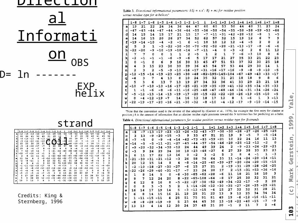
Directional Information
helix
strand
coil
Credits: King & Sternberg, 1996
OBS LOD= ln ------- EXP
104
(
c) M
ark
Ger
stei
n,
1999
, Y
ale,
bio
info
.mb
b.y
ale.
edu
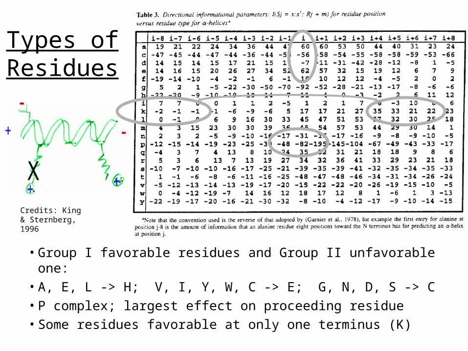
Types of Residues
• Group I favorable residues and Group II unfavorable one: • A, E, L -> H; V, I, Y, W, C -> E; G, N, D, S -> C• P complex; largest effect on proceeding residue• Some residues favorable at only one terminus (K)
Credits: King & Sternberg, 1996
105
(
c) M
ark
Ger
stei
n,
1999
, Y
ale,
bio
info
.mb
b.y
ale.
edu
GOR IV
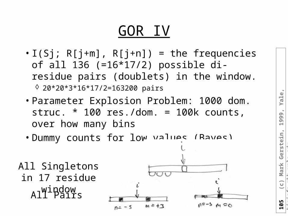
• I(Sj; R[j+m], R[j+n]) = the frequencies of all 136 (=16*17/2) possible di-residue pairs (doublets) in the window. 20*20*3*16*17/2=163200 pairs
• Parameter Explosion Problem: 1000 dom. struc. * 100 res./dom. = 100k counts, over how many bins
• Dummy counts for low values (Bayes)
All Pairs
All Singletons in 17 residue window
106
(
c) M
ark
Ger
stei
n,
1999
, Y
ale,
bio
info
.mb
b.y
ale.
edu
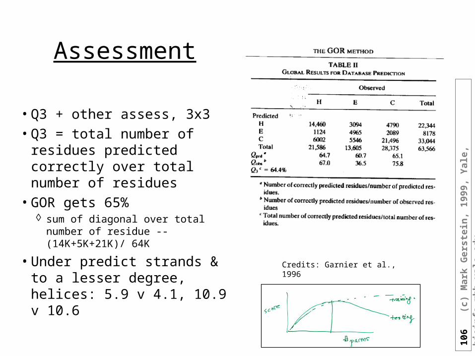
Assessment
• Q3 + other assess, 3x3• Q3 = total number of
residues predicted correctly over total number of residues
• GOR gets 65% sum of diagonal over total number
of residue -- (14K+5K+21K)/ 64K
• Under predict strands & to a lesser degree, helices: 5.9 v 4.1, 10.9 v 10.6
Credits: Garnier et al., 1996
107
(
c) M
ark
Ger
stei
n,
1999
, Y
ale,
bio
info
.mb
b.y
ale.
edu
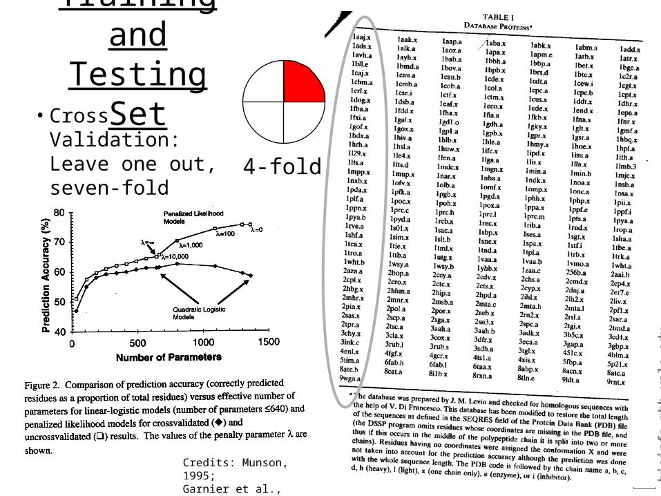
Training and Testing Set
• Cross Validation: Leave one out, seven-fold
Credits: Munson, 1995; Garnier et al., 1996
4-fold
108
(
c) M
ark
Ger
stei
n,
1999
, Y
ale,
bio
info
.mb
b.y
ale.
edu
Is 100% Accuracy Possible?
Quoted from Barton (1995):
One problem that has arisen is how to evaluate secondary structure predictions. For prediction of a single protein sequence one might expect the best residue by residue accuracy to be 100%. It is not possible to define the secondary structure of a protein exactly, however. There is always room for alternative interpretations of where a helix or strand begins or ends so failure of a prediction to match exactly the secondary structure definition is not a disaster [24]. The problem of evaluation is more complicated for prediction from multiple sequences, as the prediction is a consensus for the family and so is not expected to be 100% in agreement with any single family member. The expected range in accuracy for a perfect consensus prediction is a function of the number, diversity and length of the sequences. Russell and I have calculated estimates of this range [11].
Simple residue by residue percentage accuracy has long been the standard method of assessment of secondary structure predictions. Although a useful guide, high percentage accuracies can be obtained for predictions of structures that are unlike proteins. For example, predicting myoglobin to be entirely helical (no strand or coil) will give over 80% accuracy but the prediction is of little practical use. Rost et al. [25] and Wang [26] explore these problems and suggest some alternative measures of predictive success based on secondary structure segment overlap. Although such measures help in an objective assessment of the prediction, there is no complete substitute for visual inspection. By eye, serious errors stand out and predictions of structures that are unlike proteins are usually recognizable. By eye, it is also straightforward to weight the importance of individual secondary structures. For example, prediction of what is in fact a core strand to be a helix would seriously hamper attempts to generate the correct tertiary structure of the protein from the predicted secondary structure, whereas prediction of a non-core helix as coil may have little impact on the integrity of the tertiary structure.
109
(
c) M
ark
Ger
stei
n,
1999
, Y
ale,
bio
info
.mb
b.y
ale.
edu
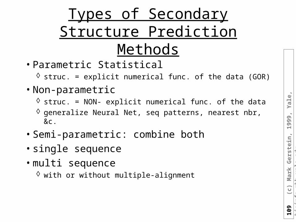
Types of Secondary Structure Prediction Methods
• Parametric Statistical struc. = explicit numerical func. of the data (GOR)
• Non-parametric struc. = NON- explicit numerical func. of the data generalize Neural Net, seq patterns, nearest nbr, &c.
• Semi-parametric: combine both• single sequence• multi sequence
with or without multiple-alignment
110
(
c) M
ark
Ger
stei
n,
1999
, Y
ale,
bio
info
.mb
b.y
ale.
edu
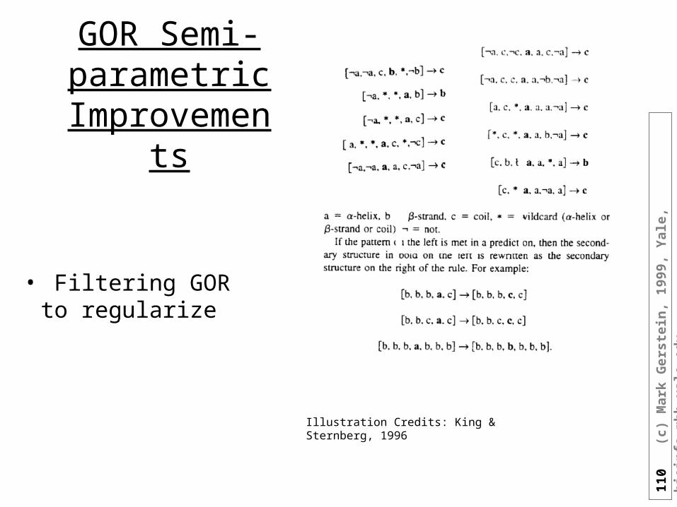
GOR Semi-parametric
Improvements
• Filtering GOR to regularize
Illustration Credits: King & Sternberg, 1996
111
(
c) M
ark
Ger
stei
n,
1999
, Y
ale,
bio
info
.mb
b.y
ale.
edu
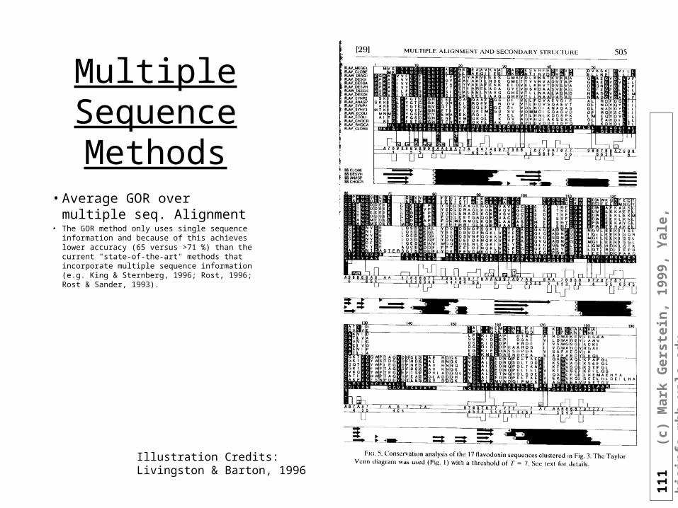
Multiple Sequence Methods
• Average GOR over multiple seq. Alignment
• The GOR method only uses single sequence information and because of this achieves lower accuracy (65 versus >71 %) than the current "state-of-the-art" methods that incorporate multiple sequence information (e.g. King & Sternberg, 1996; Rost, 1996; Rost & Sander, 1993).
Illustration Credits: Livingston & Barton, 1996
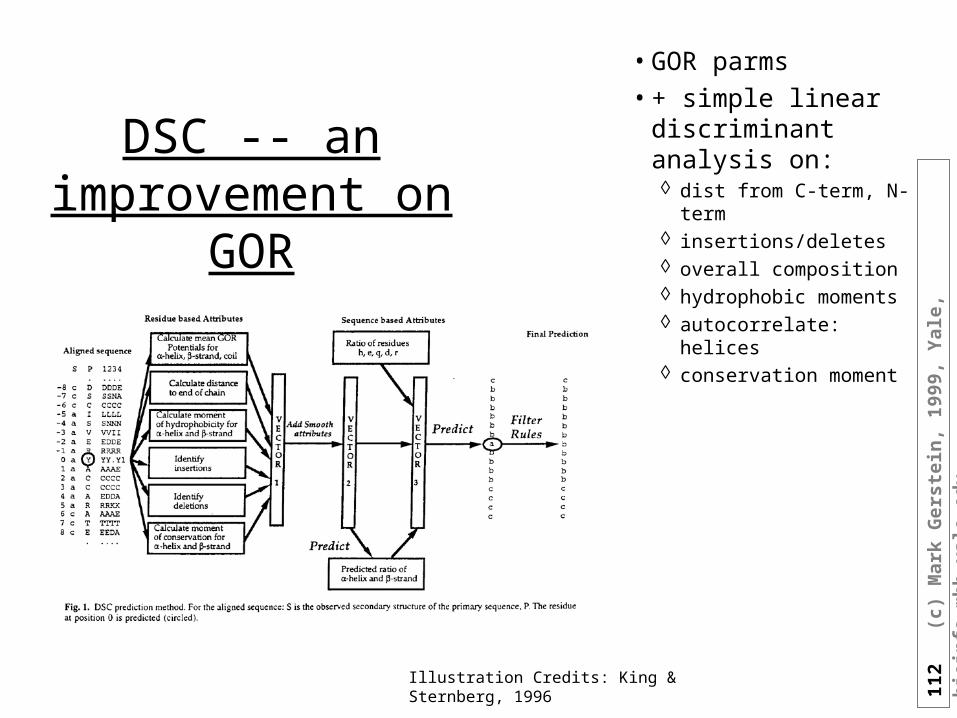
112
(
c) M
ark
Ger
stei
n,
1999
, Y
ale,
bio
info
.mb
b.y
ale.
edu
DSC -- an improvement on
GOR
• GOR parms
• + simple linear discriminant analysis on: dist from C-term, N-term insertions/deletes overall composition hydrophobic moments autocorrelate: helices conservation moment
Illustration Credits: King & Sternberg, 1996
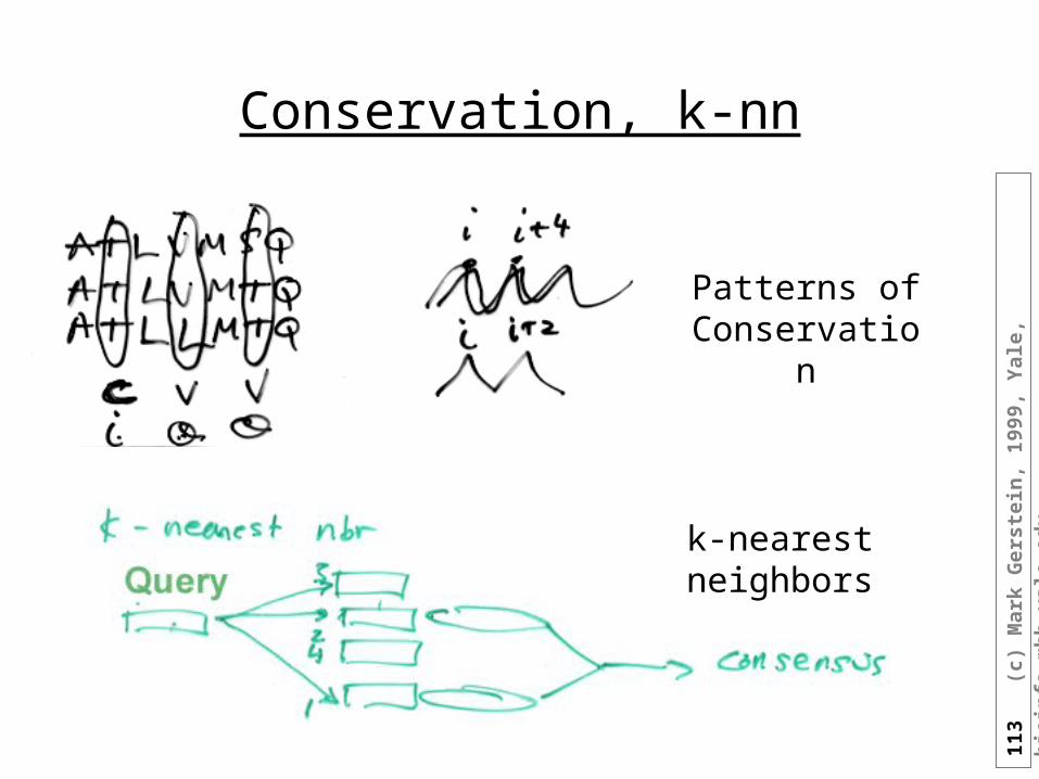
113
(
c) M
ark
Ger
stei
n,
1999
, Y
ale,
bio
info
.mb
b.y
ale.
edu
Conservation, k-nn
Patterns of Conservation
k-nearest neighbors
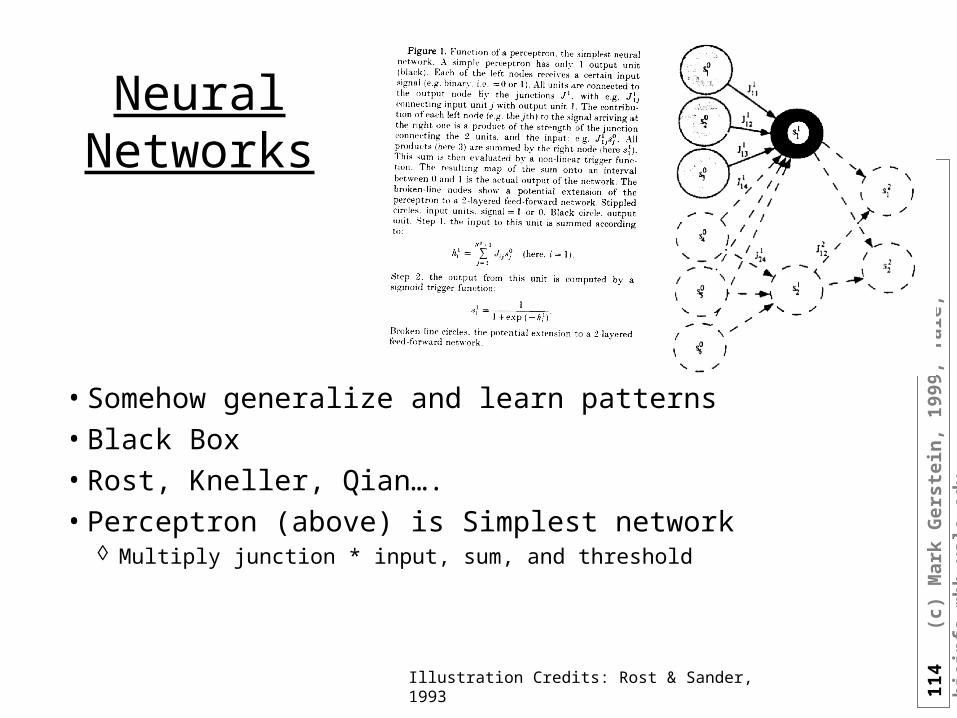
114
(
c) M
ark
Ger
stei
n,
1999
, Y
ale,
bio
info
.mb
b.y
ale.
edu
Neural Networks
• Somehow generalize and learn patterns• Black Box• Rost, Kneller, Qian….• Perceptron (above) is Simplest network
Multiply junction * input, sum, and threshold
Illustration Credits: Rost & Sander, 1993
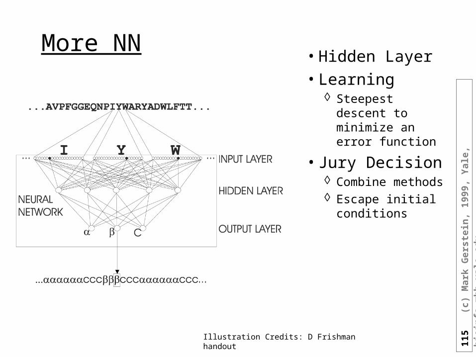
115
(
c) M
ark
Ger
stei
n,
1999
, Y
ale,
bio
info
.mb
b.y
ale.
edu
More NN• Hidden Layer• Learning
Steepest descent to minimize an error function
• Jury Decision Combine methods Escape initial
conditions
Illustration Credits: D Frishman handout
116
(
c) M
ark
Ger
stei
n,
1999
, Y
ale,
bio
info
.mb
b.y
ale.
edu
Yet more methods….
• struc class predict Vect dist. between composition vectors
• threading via pair pot• seq comparison• ab initio from md• ab initio from pair pot.
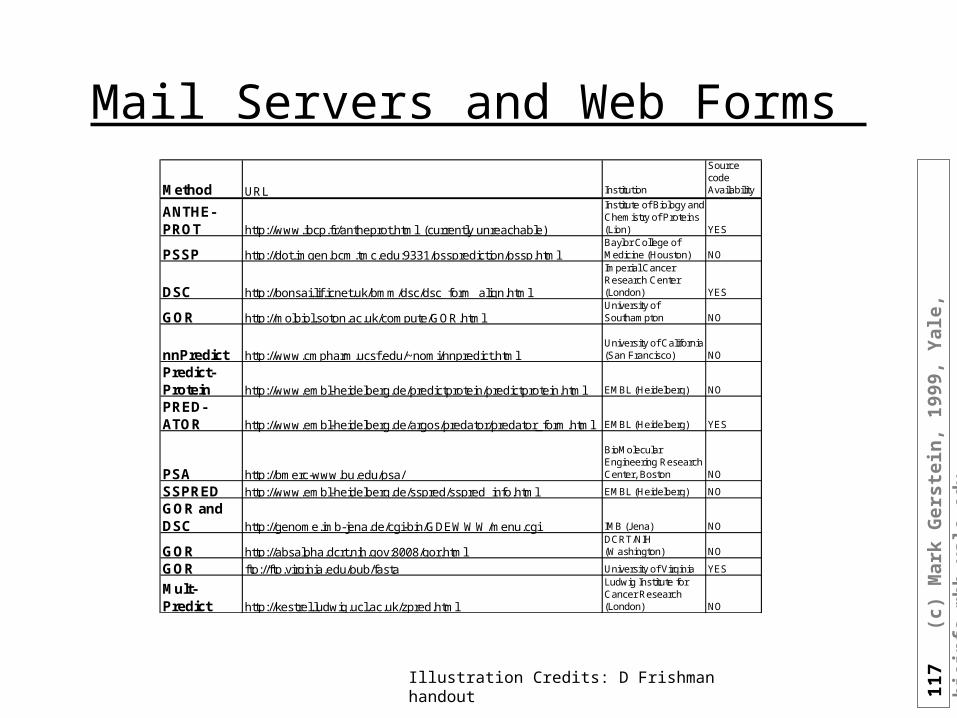
117
(
c) M
ark
Ger
stei
n,
1999
, Y
ale,
bio
info
.mb
b.y
ale.
edu
Mail Servers and Web Forms
Method URL Institution
Source code Availability
ANTHE-PROT http://www.ibcp.fr/antheprot.html (currently unreachable)
Institute of Biology and Chemistry of Proteins (Lion) YES
PSSP http://dot.imgen.bcm.tmc.edu:9331/pssprediction/pssp.html Baylor College of Medicine (Houston) NO
DSC http://bonsai.lif.icnet.uk/bmm/dsc/dsc_form_align.html
Imperial Cancer Research Center (London) YES
GOR http://molbiol.soton.ac.uk/compute/GOR.html University of Southampton NO
nnPredict http://www.cmpharm.ucsf.edu/~nomi/nnpredict.html University of California (San Francisco) NO
Predict-Protein http://www.embl-heidelberg.de/predictprotein/predictprotein.html EMBL (Heidelberg) NO
PRED-ATOR http://www.embl-heidelberg.de/argos/predator/predator_form.html EMBL (Heidelberg) YES
PSA http://bmerc-www.bu.edu/psa/
BioMolecular Engineering Research Center, Boston NO
SSPRED http://www.embl-heidelberg.de/sspred/sspred_info.html EMBL (Heidelberg) NO
GOR and DSC http://genome.imb-jena.de/cgi-bin/GDEWWW/menu.cgi IMB (Jena) NO
GOR http://absalpha.dcrt.nih.gov:8008/gor.html DCRT/NIH (Washington) NO
GOR ftp://ftp.virginia.edu/pub/fasta University of Virginia YES
Mult-Predict http://kestrel.ludwig.ucl.ac.uk/zpred.html
Ludwig Institute for Cancer Research (London) NO
Illustration Credits: D Frishman handout
118
(
c) M
ark
Ger
stei
n,
1999
, Y
ale,
bio
info
.mb
b.y
ale.
edu
Additional Features of DNA sequences in Genomes
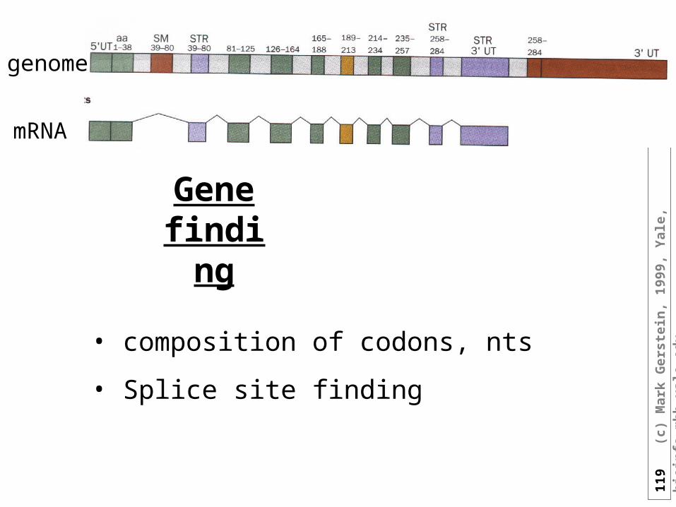
119
(
c) M
ark
Ger
stei
n,
1999
, Y
ale,
bio
info
.mb
b.y
ale.
edu
Gene finding
• composition of codons, nts
• Splice site finding
genome
mRNA
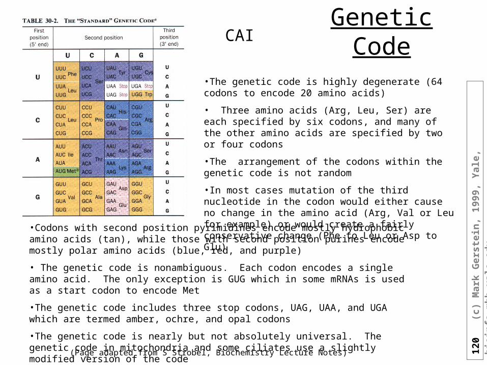
120
(
c) M
ark
Ger
stei
n,
1999
, Y
ale,
bio
info
.mb
b.y
ale.
edu
Genetic Code
•Codons with second position pyrimidines encode mostly hydrophobic amino acids (tan), while those with second position purines encode mostly polar amino acids (blue, red, and purple)
• The genetic code is nonambiguous. Each codon encodes a single amino acid. The only exception is GUG which in some mRNAs is used as a start codon to encode Met
•The genetic code includes three stop codons, UAG, UAA, and UGA which are termed amber, ochre, and opal codons
•The genetic code is nearly but not absolutely universal. The genetic code in mitochondria and some ciliates use a slightly modified version of the code
•The genetic code is highly degenerate (64 codons to encode 20 amino acids)
• Three amino acids (Arg, Leu, Ser) are each specified by six codons, and many of the other amino acids are specified by two or four codons
•The arrangement of the codons within the genetic code is not random
•In most cases mutation of the third nucleotide in the codon would either cause no change in the amino acid (Arg, Val or Leu for example) or would create a fairly conservative change (Phe to Leu or Asp to Glu)
(Page adapted from S Strobel, Biochemistry Lecture Notes)
CAI
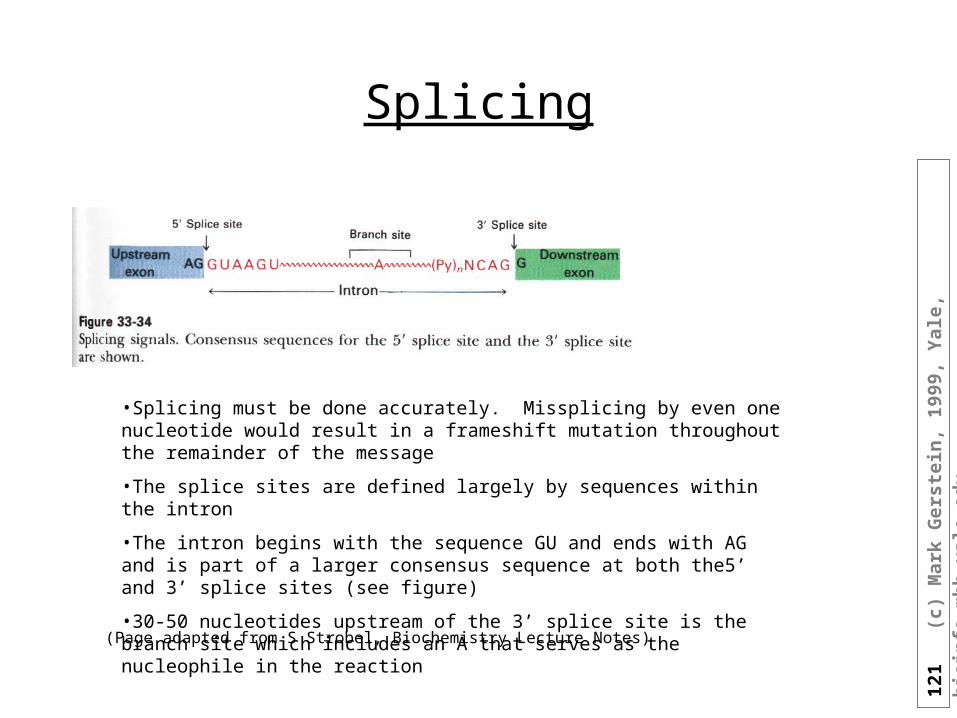
121
(
c) M
ark
Ger
stei
n,
1999
, Y
ale,
bio
info
.mb
b.y
ale.
edu
Splicing
•Splicing must be done accurately. Missplicing by even one nucleotide would result in a frameshift mutation throughout the remainder of the message
•The splice sites are defined largely by sequences within the intron
•The intron begins with the sequence GU and ends with AG and is part of a larger consensus sequence at both the5’ and 3’ splice sites (see figure)
•30-50 nucleotides upstream of the 3’ splice site is the branch site which includes an A that serves as the nucleophile in the reaction
(Page adapted from S Strobel, Biochemistry Lecture Notes)
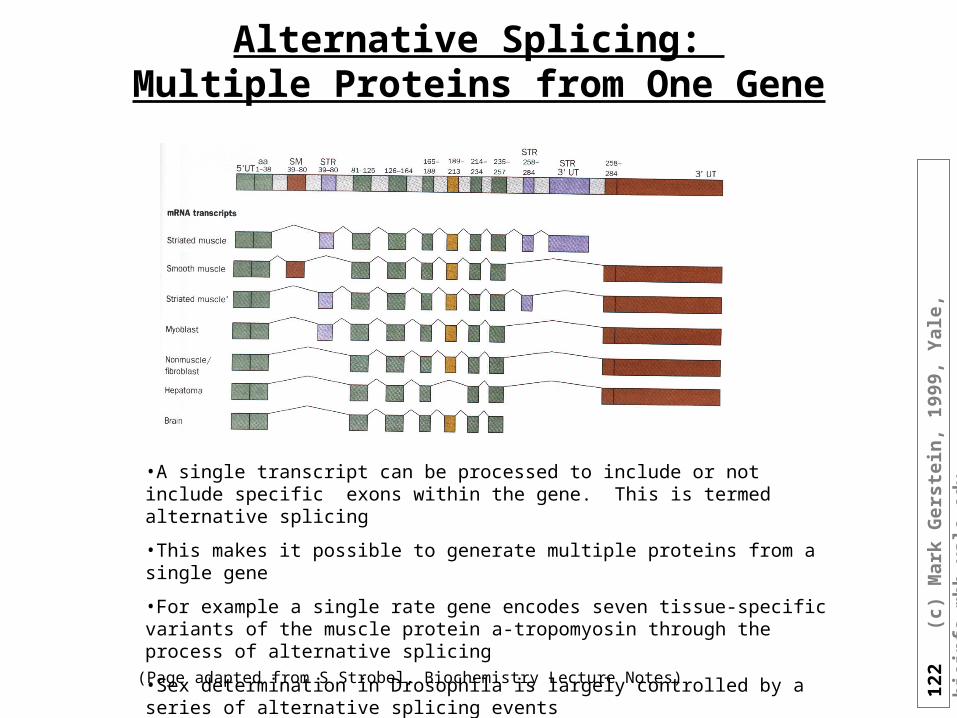
122
(
c) M
ark
Ger
stei
n,
1999
, Y
ale,
bio
info
.mb
b.y
ale.
edu
Alternative Splicing: Multiple Proteins from One Gene
•A single transcript can be processed to include or not include specific exons within the gene. This is termed alternative splicing
•This makes it possible to generate multiple proteins from a single gene
•For example a single rate gene encodes seven tissue-specific variants of the muscle protein a-tropomyosin through the process of alternative splicing
•Sex determination in Drosophila is largely controlled by a series of alternative splicing events
(Page adapted from S Strobel, Biochemistry Lecture Notes)
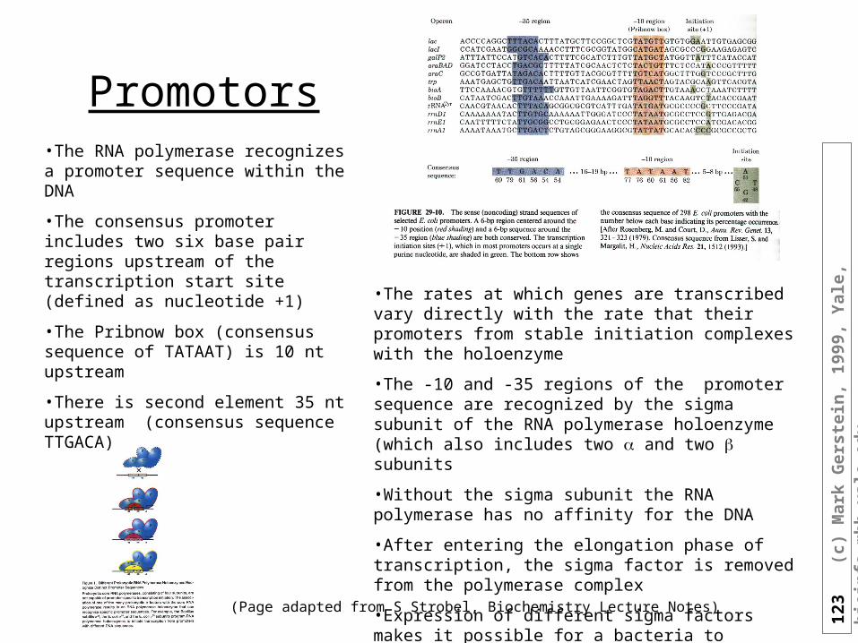
123
(
c) M
ark
Ger
stei
n,
1999
, Y
ale,
bio
info
.mb
b.y
ale.
edu
Promotors•The RNA polymerase recognizes a promoter sequence within the DNA
•The consensus promoter includes two six base pair regions upstream of the transcription start site (defined as nucleotide +1)
•The Pribnow box (consensus sequence of TATAAT) is 10 nt upstream
•There is second element 35 nt upstream (consensus sequence TTGACA)
•The rates at which genes are transcribed vary directly with the rate that their promoters from stable initiation complexes with the holoenzyme
•The -10 and -35 regions of the promoter sequence are recognized by the sigma subunit of the RNA polymerase holoenzyme (which also includes two and two subunits
•Without the sigma subunit the RNA polymerase has no affinity for the DNA
•After entering the elongation phase of transcription, the sigma factor is removed from the polymerase complex
•Expression of different sigma factors makes it possible for a bacteria to efficiently respond to external stimuli (turn on sporulation genes, heat shock genes, etc.)
(Page adapted from S Strobel, Biochemistry Lecture Notes)
124
(
c) M
ark
Ger
stei
n,
1999
, Y
ale,
bio
info
.mb
b.y
ale.
edu
ReferencesArgos P. (1976) Prediction of the secondary structure of mouse nerve growth factor and its comparison with insulin. Biochemical and Biophysical Research Communications 3:805-811.
Bairoch A and Apweiler R. (1996) The SWISS-PROT protein sequence data bank and its new supplement TREMBL. Nucleic Acids Res 24:21-25.
Barton GJ. (1995) Protein secondary structure prediction. Curr Opinion Struct Biol 5:372-376.
Benner SA, Gerloff DL, and Jenny TF. (1994) Predicting protein crystal structures. Science 265:1642-1644.
Benner SA. (1995) Predicting the conformation of proteins from sequences. Progress and future progress. J Mol Recogn 8:9-28.
Boyd, D., Schierle, C. & Beckwith, J. (1998). How many membrane proteins are there? Prot. Sci. 7, 201-205.
Crawford IP, Niermann T, and Kirschner K. (1987) Prediction of secondary structure by evolutionary comparison: application to the alpha subunit of thryptophan synthase. Proteins: Struct Func Genet 2:118-129.
Deleage G and Roux B. (1987) An algorithm for protein secondary structure prediction based on class prediction. Protein Engineering 4:289-294.
Eigenbrot C, Randal M, and Kossiakoff AA. (1992) Structural Effects Induced by Mutagenesis Affected by Crystal Packing Factors: the Structure of a 30-51 Disulfide Mutant of Basic Pancreatic Trypsin Inhibitor. Proteins 14:75.
Fasman, G. D. & Gilbert, W. A. (1990). The prediction of transmembrane protein sequences and their conformation: an evaluation. Trends Biochem Sci 15, 89-92.
Frishman D, and Argos P. (1995) Knowledge-Base Protein Secondary Structure Assignment. Proteins: Structure, Function, and Genetics 23:566-79.
Frishman D, and Argos P. (1996) Incorporation of Non-Local Interactions in Protein Secondary Structure Prediction From the Amino Acid Sequence. Protein Engineering 2:in the press.
Frishman D, and Argos P. (1997) The Future of Protein Secondary Structure Prediction Accuracy. Folding & Design 2:159-62.
Frishman, D, and P Argos. (1996) 75% Accuracy in Protein Secondary Structure Prediction. Proteins 1997 Mar;27(3):329-335 .
Garnier J and Levin JM. (1991) The protein structure code: what is its present status. Comput Appl Biosci 7:133-142.
Garnier, J. (1990). Protein structure prediction. Biochimie 72, 513-24.
Garnier, J., Gibrat, J. F. & Robson, B. (1996a). GOR method for predicting protein secondary structure from amino acid sequence. Meth. Enz. 266, 540-553.
125
(
c) M
ark
Ger
stei
n,
1999
, Y
ale,
bio
info
.mb
b.y
ale.
edu
ReferencesGarnier, J., Gibrat, J. F. & Robson, B. (1996b). GOR method for predicting protein secondary structure from amino acid sequence. Methods Enzymol 266, 540-53.
Garnier, J., Osguthorpe, D. & Robson, B. (1978). Analysis of the accuracy and implications of simple methods for predicting the secondary structure of globular proteins. J. Mol. Biol. 120, 97-120.
Geourjon C, and Deléage G. (1995) SOPMA: Significant Improvements in Protein Secondary Structure Prediction by Consensus Prediction From Multiple Sequences. Comput Appl Biosci 11:681-84.
Gibrat, J., Garnier, J. & Robson, B. (1987). Further developments of protein secondary structure prediction using information theory. J. Mol. Biol. 198, 425-443.
Gilbert RJ. (1992) Protein structure prediction from predicted residue prperties utilizing a digital encoding algorithm. J Mol Graph 10:112-119.
Holley LH, and Karplus M. (1989) Protein Secondary Structure Prediction With a Neural Network. Proc Natl Acad Sci USA 86:152-56.
Hunt NG, Gregoret LM, and Cohen FE. (1994) The origins of protein secondary structure. Effects of packing density and hydrogen bonding studied by a fast conformational search. J Mol Biol 241:214-225.
Kabsch W and Sander C. (1984) On the use of sequence homologies to predict protein structure. Identical pentapeptides can have completely different conformation. Proc Natl Acad Sci USA 81:1075-1078.
Kabsch W, and Sander C. (1983) Dictionary of Protein Secondary Structure: Pattern Recognition of Hydrogen-Bonded and Geometrical Features. Biopolymers 22:2577-637.
Kendrew JC, Klyne W, Lifson S, Miyazawa T, Nemethy G, Phillips DC, Ramachandran GN, and Sheraga HA. (1970). Biochemistry 9:3471-79.
King, R. D. & Sternberg, M. J. E. (1996). Identification and application of the concepts important for accurate and reliable protein secondary structure prediction. Prot. Sci. 5, 2298-2310.
King, R. D., Saqi, M., Sayle, R. & Sternberg, M. J. (1997). DSC: public domain protein secondary structure predication. Comput Appl Biosci 13, 473-4.
Levin J, Pascarella S, Argos P, and Garnier J. (1993) Quantification of secondary structure prediction improvement using multiple alignments. Protein Engineering 6:849-854.
Levin JM, Robson B, and Garnier J. (1986) An algorithm for secondary structure determination in proteins based on sequence similarity. FEBS Lett 205:303-308.
Levitt M, and Greer J. (1977) Automatic Identification of Secondary Structure in Globular Proteins. J Mol Biol 114:181-239.
Lim VI. (1974) Algorithms for prediction of alpha-helical and beta-structural regions in globular proteins. J Mol Biol 88:873-894.
Livingstone CD, Barton GJ (1996). Identification of functional residues and secondary structure from protein multiple sequence alignment. Methods Enzymol 266:497-512
Lupas A, Koster AJ, Walz J, and Baumeister W. (1994) Predicted secondary structure of the 20 S proteasome and model structure of the putative peptide channel. FEBS Lett 354:45-49.
Matthews B. (1975) Comparison of the predicted and observed secondary structure of T4 phage lysozyme. Biochem Biophys Acta 405:442-451.
Mehta PK, Heringa J, and Argos P. (1995) A simple and fast approach to prediction of protein secondary structure from multiply aligned sequences with accuracy above 70%. Protein Science 4:2517-2525.
126
(
c) M
ark
Ger
stei
n,
1999
, Y
ale,
bio
info
.mb
b.y
ale.
edu
ReferencesMuggleton S, King RD, and Sternberg MJE. (1992) Protein Secondary Structure Prediction Using Logic-Based Machine Learning. Protein Engineering 5:647-57.
Nishikawa K, and Ooi T. (1986) Amino Acid Sequence Homology Applied to the Prediction of Protein Secondary Structures, and Joint Prediction With Existing Methods. Biochimica Et Biophysica Acta 871:45-54.
Pauling L, Corey RB, and Branson HR. (1951) The structure of proteins: two hydrogen-bonded helical configurations of the polypeptide chain. Proc Natl Acad Sci USA 37:205-211.
Persson, B. & Argos, P. (1997). Prediction of membrane protein topology utilizing multiple sequence alignments. J Protein Chem 16, 453-7.
Presnell SR, Cohen BI, and Cohen FE. (1992) A segment-based approach to protein secondary structure prediction. Biochemistry 31:983-993.
Ptitsyn OB and Finkelstein AV. (1983) Theory of protein secondary structure and algorithm of its prediction. Biopolymers 22:15-25.
Qian N, and Sejnowski TJ. (1988) Predicting the Secondary Structure of Globular Proteins Using Neural Network Models. J Mol Biol 202:865-84.
Rackovsky S. (1993) On the nature of the protein folding code. Proc Natl Acad Sci U S A 90:644-648.
Ramakrishnan C, and Soman KV. (1982) Identification of Secondary Structures in Globular Proteins - a New Algorithm. Int J Pept Protein Res 20:218-37.
Rao S, Zhu Q-L, Vaida S, and Smith T. (1993) The local information content of the protein structural database. FEBS Lett 2:143-146.
Rice CM, Fuchs R, Higgins DG, Stoehr PJ, and Cameron G N. (1993) The EMBL data library. Nucleic Acids Res 21:2967-2971.
Richards FM, and Kundrot CE. (1988) Identification of Structural Motifs From Protein Coordinate Data: Secondary Structure and First-Level Supersecondary Structure. Proteins: Struct Func Genet 3:71-84.
Robson B, and Garnier J. (1993) Protein Structure Prediction. Nature 361:506.
Rost B, and Sander C. (1993) Prediction of Protein Secondary Structure at Better Than 70% Accuracy. J Mol Biol 232:584-99.
Rost B, Sander C, and Schneider R. (1994) Redefining the goals of protein secondary structure prediction. J Mol Biol 235:13-26.
Rost B, Sander C. (1993) Improved prediction of protein secondary structure by use of sequence profiles and neural networks. Proc Natl Acad Sci USA 90:7558-7562
Rost, B., Schneider, R. & Sander, C. (1993). Progress in protein structure prediction? Trends Biochem Sci 18, 120-3.
Rumelhart DE, Hinton GE, and Williams R. (1986) Learning representations by back-propagating errors. Nature 323:533-536.
Salamov AA, and Solovyev VV. (1995) Prediction of Protein Secondary Structure by Combining Nearest-Meighbour Akgorithms Amd Multiple Sequence Alignments. J Mol Biol 247:11-15.
Salamov AA, and Solovyev VV. (1997) Protein Secondary Structure Prediction Using Local Alignments. Journal of Molecular Biology 268:31-36.
Sayle RA, and Milner-White EJ. (1995) RASMOL: Biomolecular Graphics for All. Trends in Biochemical Sciences 20:374-76.
127
(
c) M
ark
Ger
stei
n,
1999
, Y
ale,
bio
info
.mb
b.y
ale.
edu
ReferencesSayle RA, and Milner-White EJ. (1995) RASMOL: Biomolecular Graphics for All. Trends in Biochemical Sciences 20:374-76.
Sklenar H, Etchebest C, and Lavery R. (1989) Describing Protein Structure: a General Algorithm Yielding Complete Helicoidal Parameters and a Unique Overall Axis. Proteins: Struct Func Genet 6:46-60.
Solovyev VV and Salamov AA. (1994) Predicting alpha-helix and beta-strand segments of globular proteins. Comput Appl Biosci 10:661-669.
Stolorz P, Lapedes A, and Xia Y. (1992) Predicting Protein Secondary Structure Using Neural Net and Statistical Methods. J Mol Biol 225:363-77.
Sumpter BG, Getino C, and Noid DW. (1994) Theory and applications of neural computing in chemical science. Ann Rev phys Chem 45:439-481.
Sumpter BG, Getino C, and Noid DW. (19949 Theory and applications of neural computing in chemical science. Ann Rev phys Chem 45:439-481.
Taylor WR and Thornton JM. (1984) Recognition of super-secondary structure in proteins. J Mol Biol 173:487-5141984.
Thompson JD, Higgins DG, and Gibson TJ. (1994) CLUSTAL W: improving the sensitivity of progressive multiple sequence alignment through sequence weighting, position-specific gap penalties and weight matrix choice. Nucleic Acids Res 22:4673-4680.
Thornton JM, Flores TP, Jones DT, and Swindells MB. (1991) Prediction of progress at last. Nature 354:105-106.
von Heijne, G. (1992). Membrane protein structure prediction. Hydrophobicity analysis and the positive-inside rule. J Mol Biol 225, 487-94.
Wasserman PD. (1989) Neural Computing. Theory and Practice. New York.
Zhang X, Mesirov JP, and Waltz DL. (1992) Hybrid System for Protein Secondary Structure Prediction. J Mol Biol 225:1049-63.
Zvelebil MJ, Barton GJ, Taylor WR, and Sternberg MJ. (1987) Prediction of Protein Secondary Structure and Active Sites Using the Alignment of Homologous Sequences. J Mol Biol 195:957-61.
128
(
c) M
ark
Ger
stei
n,
1999
, Y
ale,
bio
info
.mb
b.y
ale.
edu
End of Class 4 with 15’ left