an integrated programming and development environment · pdf filean integrated programming and...
TRANSCRIPT
An Integrated Programming and DevelopmentEnvironment for Adiabatic Quantum Optimization
T S Humble A J McCaskeydagger R S Bennink J J BillingsE F DrsquoAzevedo B D SullivanDagger C F Klymkosect H SeddiqiQuantum Computing Institute Oak Ridge National Laboratory Oak Ridge TNUSA
E-mail humbletsornlgov
Abstract Adiabatic quantum computing is a promising route to thecomputational power afforded by quantum information processing The recentavailability of adiabatic hardware has raised challenging questions about how toevaluate adiabatic quantum optimization programs Processor behavior dependson multiple steps to synthesize an adiabatic quantum program which areeach highly tunable We present an integrated programming and developmentenvironment for adiabatic quantum optimization called JADE that providescontrol over all the steps taken during program synthesis JADE capturesthe workflow needed to rigorously specify the adiabatic quantum optimizationalgorithm while allowing a variety of problem types programming techniquesand processor configurations We have also integrated JADE with a quantumsimulation engine that enables program profiling using numerical calculation Thecomputational engine supports plug-ins for simulation methodologies tailored tovarious metrics and computing resources We present the design integration anddeployment of JADE and discuss its potential use for benchmarking adiabaticquantum optimization programs by the quantum computer science community
dagger Present address Department of Physics Virginia Tech Blacksburg VA USADagger Present address Department of Computer Science North Carolina State University Raleigh NCUSAsect Present address Department of Mathematics and Computer Science Emory University AtlantaGA USA Present address Department of Physics Georgia Southern University Statesboro GA USA
arX
iv1
309
3575
v3 [
quan
t-ph
] 2
1 A
pr 2
014
CONTENTS 2
Contents
1 Introduction 2
2 Adiabatic Quantum Programming 521 Quantum Computational Model 522 Adiabatic Quantum Optimization 623 Quadratic Unconstrained Binary Optimization 624 Hardware Embedding 725 Hardware Schedules and Program Execution 926 Computational Readout and Problem Solution 10
3 Jade Adiabatic Development Environment 1031 Use Cases 1132 System Context 1233 Component Architecture 1334 JadeD 1335 NiCE 1836 Sapphire 1937 Simulation Plug-ins 2038 Testing Framework 22
4 Usage Example 22
5 Discussion 26
1 Introduction
The discovery of quantum algorithms with significant speed-ups over their classicalcounterparts has spurred interest in the research and development of quantumcomputing systems [1] Several different but computationally equivalent models forquantum computing have emerged including in particular the model of adiabaticquantum computing (AQC) [2 3] Notionally the AQC model for universal quantumcomputation corresponds to adiabatic (ie slow) changes in the state of a quantumphysical system While computationally equivalent to other models AQC promisessome intrinsic benefits for ensuring fault-tolerant computation and reducing systemcomplexity [4 5 6]
Additional attention to the AQC model has been stimulated by the recentcommercial realization of a special purpose processor that implements the adiabaticquantum optimization (AQO) algorithm [7 2 3] The processor manufactured by thecompany D-Wave Systems Inc realizes a programmable Ising spin-glass model in atransverse field [8 9 10 11 12] This hardware is specialized to the AQO algorithmand it is not capable of universal computation within the AQC model but it doesprovide a complete realization of a quantum computational device This has spurredvigorous scientific studies into exactly how the current hardware performs quantumcomputation including efforts to differentiate its observed behavior from classicalphysical processes [13 14] Moreover the AQO algorithm is broadly applicableto combinatorial optimization problems and consequentlt the D-Wave processorhas garnered attention for its potential use in a number of application domains
CONTENTS 3
Examples include problems in classification [15 16] machine learning [17] graphtheory [18 19 20] artificial neural networks [21] and protein folding [22] amongothers [23]
The availability of quantum hardware allows for benchmarking performancerelative to both quantum and classical metrics of computational power Understandingobserved behavior requires a detailed consideration of how the program and hardwareinteract as well as how the defined metrics represent performance For example itis known that performance of the AQO algorithm depends strongly on the specificprogramming and hardware operation schedules as well as the problem input [24 25]Indeed whereas some studies of the AQO algorithm have reported runtimes thatscale polynomially in problem size [26 2 27 28] others have suggested worst-case exponential behavior or trapping in local minima [29] More generally it hasproven difficult to predict the run times of particular problem instances due to thecomplexity of the underlying quantum dynamics An essential step in understandingthese behaviors is to capture the influence that different programming choices have onobserved run times [7 30 29 31 32 33 34 35 36]
Figure 1 A flowchart highlighting the multiple steps taken to synthesize anadiabatic quantum program for the AQO algorithm The steps are elaborated indetail in Sec 2 Briefly a QUBO problem serves as the classical input to programsynthesis while the computed QUBO solution represents the value returned bythe program Each block in the diagram corresponds to a distinct intermediaterepresentation of the quantum program that depends on the choices made in theprevious steps
A significant source of the complexity in analyzing implementations of the AQOalgorithm arises from the multiple steps undertaken to synthesize the adiabaticquantum program We provide a brief summary of the process with elaborationof the detailed synthesis deferred to Sec 2 Figure 1 illustrates that an adiabaticquantum programming process begins with the reduction of a classical combinatorialoptimization problem to a quadratic unconstrained binary optimization (QUBO)problem The QUBO problem is then mapped into the parameters of an equivalentlogical Ising Hamiltonian The logical Ising Hamiltonian must then be mapped ontothe processor as a physical Ising Hamiltonian a process defined as embedding Thistransformation of the reduced problem into a physically realizable program dependson both the hardware layout and the available hardware controls Ultimately thecomputed solution will depend on all previous decisions as well as the actual physics
CONTENTS 4
underlying the processorIt is currently poorly understood how modifications at the various stages in Fig 1
impact the correctness and efficacy of computed solutions Reconciling the seeminglycontradictory results from previous studies as well as understanding more recentexperimental benchmarks requires investigating how programming choices impactperformance Motivated by this we have developed a software environment thatcaptures each step in deriving a program for the adiabatic quantum optimizationalgorithm Our framework does not address programming for a universal adiabaticquantum computer but instead it is specialized to the AQO algorithm and theIsing spin-glass physics underlying the D-Wave processors The software synthesizestogether the steps from Fig 1 into an integrated workflow that includes thedevelopment of adiabatic quantum programs as well as the collection of diagnosticinformation for addressing questions about performance In the absence of actualhardware we use numerical simulation to evaluate the variety of programming andoperational choices that can effect program behavior Our simulation capabilitiesemploy multiple numerical methods with the possibility for user extensions Anotherimportant part of the framework is the ability to analyze both the solutions recoveredby simulations as well as the intermediate dynamics and Hamiltonians With thepublication of recent benchmarks from available hardware [35 34 37] the abilityto make comparisons between simulated and experimental results can be useful forunderstanding observed behavior
The Jade Adiabatic Development Environment (JADE) implements theprogramming steps highlighted in Fig 1 JADE capabilities include capturing inputfor a high-level optimization QUBO problem as well as generating the low-levelquantum physical program representation JADE is further integrated with a quantumsimulation engine that supports user-defined methodologies for running diagnosticanalyses We present explicit examples of several simulations methodologies based onfinite differencing as well as diagnostic derived from the time-dependent eigenspectraand eigenstate populations
Because the JADE programming model is tailored to the AQO algorithm andIsing spin glass physics we suggest that JADE may be useful supporting ongoingbenchmark studies of the D-Wave System processor We do not address the issue ofdeveloping benchmarks or methods of evaluating quantum program efficiency but wedo provide a concrete realization of the integrated computational environment neededto carry out such efforts In particular our development environment formalizesmethods used for programming the quantum processor while offering an interfaceto simulation for computing detailed diagnostics about how a program executes Forcompleteness we note that there is some superficial similarity between JADE and theproprietary BlackBox Compiler from D-Wave Systems which provides an interfacefor solving problems on hardware The primary distinction of JADE is that it enablesexplicit control of the programming steps for the purpose of testing new programmingtechniques Conceptually a JADE program could be used to drive the actual quantumprocessor by interfacing with the hardware control system but we have not exploredthat option here
This paper is organized as follows In Sec 2 we summarize the theoreticalbackground leading to Fig 1 including the quantum physical basis for AQO InSec 3 we present the model-based design of JADE including the system contextimplementations of each component and our test-driven framework for programverification and validation We present usage results for the case of a recent benchmark
CONTENTS 5
problem in Sec 4 and we offer conclusions in Sec 5
2 Adiabatic Quantum Programming
In this section we provide a summary of the physical theory and computer scienceunderlying adiabatic quantum programming This includes the quantum physicaldescription of AQC as well as the steps taken to map the AQO algorithm to a hardwarecontrol schedule
21 Quantum Computational Model
The physical basis for the AQC model was first established in terms of quantumannealing by Kadowaki and Nishimori [38] Farhi et al as well as others laterformalized these ideas as a means of universal computation [7 2 39] Severalefforts have since shown the equivalence between the AQC model and other quantumcomputing models [40 41] In a generalized AQC algorithm [7 2 3] a quantumphysical system of n qubits is evolved under the Schrodinger equation
ihpart |ψ(t)〉partt
= H(t) |ψ(t)〉 (1)
according to a time-dependent Hamiltonian
H(t) = A(t)HI +B(t)HP (2)
that interpolates between the initial Hamiltonian HI and the final (problem)Hamiltonian HP from an initial time t = t0 to a final time t = T We shall assumet0 = 0 In Eq (2) the schedules A(t) and B(t) satisfy the boundary conditionsA(0) B(0) and A(T ) B(T ) while the quantum system is initially prepared inthe lowest-energy eigenstate of HI Given the instantaneous eigenvalue equations
H(t)∣∣∣φj(t)rang = Ej(t)
∣∣∣φj(t)rang (3)
with j = 0 1 2n minus 1 labeling states of monotonically increasing energy the initial
state condition implies |ψ(0)〉 =∣∣∣φ0(0)
rang
We define the energy gap between the ground and first excited state as
∆(t) = E1(t)minus E0(t) (4)
in which we neglect possible ground state degeneracy for simplicity If the energy gapis always strictly greater than zero ie forallt ∆(t) gt 0 then the state |ψ(t)〉 will remainin the instantaneous ground state with high probability provided certain bounds onthe rate of change of the Hamiltonian are satisfied [2] Consequently evolution underEq (1) to the time T prepares the final state |ψ(T )〉 in the lowest energy eigenstateof HP By making a judicious choice of the final Hamiltonian HP the prepared finalstate may encode the solution to a computation In order to ensure the computationis correct the adiabatic condition must be satisfied In its simplest interpretationthis implies the global time T must be much larger than the inverse of the minimumspectral gap of H(t) [2] More sophisticated analysis shows that better results may beobtained by adjusting the evolution schedule according to the local energy gap [30]In either case failure to ensure the adiabatic condition risks the possibility that thefinal state will not belong to the ground state manifold of HP but rather to an excitedstate and an error in the computation It is notable that the spectral gap depends not
CONTENTS 6
only on the problem to be solved but also on how the problem is implemented as aquantum program Understanding input influence on a program run time and errorrates is an open question in quantum computer science
22 Adiabatic Quantum Optimization
In specializing to the AQO algorithm we require a quantum logical system of n qubitswith an initial Hamiltonian
HI = minussumiisinVP
Xi (5)
and final Ising Hamiltonian
HP = minussumiisinVP
αiZi minussum
(ij)isinEP
βijZiZj (6)
where Xi and Zi are the Pauli operators for the i-th qubit [1] αi is the bias on the i-thqubit and βij is the coupling between qubits i and j As shown in the section belowthe graph GP = (VP EP ) with vertex set VP (|VP | equiv n) and edge set EP defines aninput optimization problem cf the weight matrix P in Eq (7) The final Hamiltonianis diagonal in the basis defined by the tensor products of the plusmn1 eigenstates of the Zi
operators This basis will also serve as the computational basis For comparison theground state of the initial Hamiltonian (and initial state of the AQO algorithm) is thesymmetric superposition of these computational basis states and has an eigenvalueminusn
An important consequence arising from the choice of the initial and finalHamiltonians respectively Eqs (5) and ( 6) is that the time-dependent HamiltonianH(t) of Eq (2) is not capable of universal adiabatic quantum computation Extendingthe form of the Hamiltonian beyond the Ising model for example to the 2-local ZZXXHamiltonian of Biamonte and Love [42] would support universal computation but wedo not consider that case here
23 Quadratic Unconstrained Binary Optimization
Any binary optimization problem (BOP) can be mapped into the form of the finalHamiltonian in Eq (6) In doing so we define the classical input to the AQO algorithmas a quadratic unconstrained binary optimization (QUBO) problem This is becausenon-binary as well as constrained optimization problems can be reduced to QUBO[43] with multiple methods for performing the reduction available [44] The QUBOproblem is to find
arg minxisinBm
xTPx (7)
where x is a vector of n binary variables with xi isin 0 1 and P is an n-by-n symmetricreal-valued cost matrix We use the weight matrix P to define the weighted adjacencymatrix of the input (problem) graph GP introduced in Eq (6) The graph GP has avertex set VP of size |VP | equiv n and an edge set EP defined as (i j) isin EP iff Pij 6= 0From this point of view programming the AQO algorithm requires mapping the matrixP to the biases and couplings of the Ising Hamiltonian It has been shown previously
CONTENTS 7
by Choi that parameterization of the logical Ising Hamiltonian in Eq (6) may be givenin terms of the QUBO problem as [24]
αi =1
2Pii +
1
4
nsumj=1
Pij for i = 1 to n (8)
and
βij =1
4Pij for i lt j = 1 to n (9)
We may also add an energy shift to the Ising Hamiltonian in Eq (6) of the form
γ =1
4
nsumij=1
Pij +1
2
nsumi=1
Pii (10)
in order to match the energies of the solution state Although this shift does not affectthe solution obtained using AQC it must be accounted for in reporting the minimalvalue in Eq (7)
24 Hardware Embedding
Whether or not the logical Hamiltonian in Eq (6) is supported directly on a givenhardware depends on the available connectivity of that hardware We express theconnectivity of a targeted processor in terms of its hardware graph GH = (VH EH)When any vertex can be coupled to any other vertex and |VH | ge |VP | then it ispossible to support all possible input problems using a one-to-one mapping between thelogical and physical qubits and the biases and couplings of the physical HamiltonianHowever when GH is less than fully connected then there are certain input problemsthat will not map directly into hardware In such circumstances it may be possible toembed the problem graph GP into the hardware graph GH via graph minor embedding[45 25]
We formally define the minor embedding of a graph GP into a graph GH as amapping φ VP rarr VH such that
(i) each vertex i in VP is mapped to the vertex set of a connected subgraph Ti ofGH
(ii) if (i j) isin EP then there exist τi τj isin VH such that τi isin Ti τj isin Tj and(τi τj) isin EH
If such a mapping φ exists then GP is minor-embeddable in GH or GP is a minor ofGH In subsequent discussions we simply use the term embedding as a reference tominor embedding
In adiabatic quantum programming the vertices of the input graph GP representthe bits of a candidate solution to the QUBO problem while the edges represent thepresence of nonzero coupling coefficients as defined in Eqs (8) and (9) respectivelyThe vertices of the hardware graph GH represent the physical qubits and the edgesrepresent the couplings between qubits that are available in the hardware Anembedding maps each vertex in VP to a subset of VH and each edge in EP toedges between these subsets When an embedding exists then the resulting subgraphGlowast = (V lowast Elowast) of the hardware graph defines the physical Ising model
HGlowast = minussumkisinV lowast
αlowastkZk minussum
(k`)isinElowast
βlowastk`ZkZ` (11)
CONTENTS 8
The bias and coupling coefficients αlowastk and βlowastk` depend on the selected embedding φ perthe requirements (i) and (ii) listed above The physical Ising coefficients are definedas [45]
αlowastk = αi|Ti| for each k isin VTi(12)
and for k 6= `
βlowastk` =
βijedges(Ti Tj) for k isin Ti and ` isin Tj and i 6= jJ for k isin Ti and ` isin Tj and i = j0 otherwise
(13)
where edges(Ti Tj) is the number of edges between subgraphs Ti and Tj The constantJ is chosen sufficiently large to force the qubits in each subgraph to be stronglycorrelated with an upper bound on its value given previously by Choi [45] Settingthe embedded Ising model coefficients requires knowledge of the matrix P and theselected embedding implied by Glowast [45 25] The embedding need not be unique andconsequently different instances of the Hamiltonian in Eq (11) may correspond tothe same logical problem of Eq (7)
A key dependency in finding an embedding is the target hardware graph GH The hardware graph defines the vertices and connectivity that are available to expressthe Ising model An example hardware graph is shown in Fig 2 Finding thosegraphs that can be embedded into a fixed hardware graph is an example of subgraphisomorphism which is known to be NP-Complete in difficulty [46] For small hardwaregraphs it is tractable to calculate the maximal minors of the graph ie the minorsof GH whose subgraphs represent all other graphs contained in GH [25] Howeverthis is a brute force approach and therefore does not scale favorably with hardwaresize Similarly attempts to find complete graphs as minor of an arbitrary hardwaregraph as known to be NP-Complete [47] Alternatives to these brute force approachesinclude heuristic algorithms that incorporate knowledge of GH or that limit the typesof input problems [25]
At this point we emphasize that the role of minor embedding is not as simpleas identifying a physical Ising model that is equivalent to the logical HamiltonianIndeed the embedding of a problem into a processor is not unique and moreover itis not well understood how different embeddings influence program behavior Thereare known tradeoffs in the amount of time spent finding an embedding relative to thesize of the embedded problem [25] but it remains unclear how to account for thosecosts in the benchmarking program performance
In addition the current approach to hardware embedding taken by JADE followsthe decomposition of a BOP into a QUBO form using quadratization ie decomposinginto quadratic form [44] However an alternative programming sequence is to mapa BOP directly into a multi-linear Ising model that is then decomposed into bilinearform [48] The latter approach has led to the development of generalized gadgets[49] and more recently to resource efficient gadgets that replace multi-linear termsin the Hamiltonian with bilinear ones [50 51 52] Gadget decompositions introduceadditional ancilla qubits in much the same way that quadratization introduces ancillabits Biamonte has presented decompositions minimal in the number of gadget ancillathat would be especially relevant to comparing performance [50] We have not exploredthe use of gadgets in the JADE programming model or compared the overhead usingquadratization but we believe that the impact of this alternative programming modelshould be investigated
CONTENTS 9
Figure 2 A hardware graph for the Rainier processor produced by D-WaveSystems Inc The design is a 4times 4 lattice of interconnected unit cells with eachunit cell is expressed as a K44 graph The more recent Vesuvius processor has asimilar design using an 8times 8 lattice of unit cells The geometry of the hardwareplays an important role in determining which graphs can be embedded
25 Hardware Schedules and Program Execution
We restrict our discussion to AQO algorithms that use a time-dependent Hamiltonianfitting the form of Eq (2) which interpolates between an initial Hamiltonian HI andthe problem Hamiltonian HP according to the time-dependent annealing schedulesA(t) and B(t) More generally individual biases and couplings can be time-dependenteg αi = αi(t) In either case the time-dependent schedules specify the rate at whichthe total Hamiltonian H(t) changes and consequently they play an important role inthe computational error rates In particular the final time T needs to be sufficientlylarge to ensure the validity of the adiabatic condition namely
T E∆lowast
(14)
where ∆lowast = mint ∆(t) is the global minimum of the spectral gap defined in Eq (4)and E = maxt〈dH(t)dt〉 is the maximal rate of change during evolution [2] In theabsence of information about ∆(t) it is difficult to ensure the adiabatic condition issatisfied This uncertainty is one source of the difficulty in benchmarking adiabaticquantum programs Recent results on amplifying spectral gaps [53] and developingfault tolerant programs [54] suggest new methods for mitigating this uncertainty
Although the annealing schedules are sufficient for coarsely specifying programexecution it is ultimately necessary to provide the physical implementation of thoseschedules in terms of hardware controls The hardware controls that are availablefor tuning the biases and coupling of a processor must be capable of expressingprogrammed schedules However available controls are highly dependent on thephysics underlying a processor and ensuring the exact implementation of an arbitraryannealing schedule may not be possible Limitations on annealing schedules arisingfrom constraints and dependencies of control values creates additional uncertainty in
CONTENTS 10
the benchmarking effort Accounting for control constraints and quantification noiseis necessary to provide a clear picture of how processor differences impact programbehavior For example in the case of the family of processors from D-Wave SystemsInc biases and couplings can be mapped directly to models for the underlyingsuperconductor Josephson-junction However the precision of this mapping is limitedby the resolution of the on-board digital to analog converters (DACrsquos) [8 10]
In addition to the constraints expected from hardware design it is also necessaryto anticipate the influence of noise on program behavior Two types of noise affectingquantum dynamics are classical noise in the controls and quantum noise in the systemdynamics Quantum noise may be modeled as an undesired interaction betweencomputational qubits and non-control elements of the hardware A specific exampleis the case of thermal influences on the quantum dynamics which invalidate the purestate description in Sec 2 and undermine the adiabatic conditions [55] Similarlyclassical noise in the hardware controls yields a mixed-state description of the quantumdynamics and may bias program execution away from the solution of interest
Once the time-dependent behavior of the Hamiltonian H(t) has been fullyspecified it remains to execute the program As noted before the typical sequencebegins by initializing the quantum computational register in the ground state of theinitial Hamiltonian HI How initialization is implemented varies with processor andmore important it may not be implemented perfectly This additional source of noisemust also be accounted for in evaluating program behavior as it is likely to influencethe computational result The remaining step in execution is to carry out the hardwarecontrol schedule and therefore the programmed computation
26 Computational Readout and Problem Solution
After evolving to the final time T the state of the computational register is determinedusing a suitable measurement or readout method For the case of the AQO algorithmthe ground states at time T are computational eigenstates and therefore readoutimplies a direct measurement in the computational (Z) basis As with programexecution it is more realistic to describe the readout process in terms of thehardware controls This description includes capturing any noise or uncertainty inthe measurement process
The bit string generated from computational readout is the result of the quantumannealing process However mapping this result back to a solution for the originalQUBO problem requires decoding measurements according to the inverse of theembedding map For those cases where a tree of physical qubits represents a singlelogical qubit it is necessary to check the value of all such qubits In cases wheremeasurement results within a tree disagree then various strategies can resolve theuncertainty One simple example is to use a majority vote After decoding thecomputational readout a solution to the original QUBO problem is produced andthe program is complete It may be necessary to repeat the execution of the programfor example to gather statistics on the readout or solution states however the stepsperformed are similar to those described above
3 Jade Adiabatic Development Environment
As presented in Sec 2 programming the AQO algorithm for an arbitrary QUBO is ahighly tunable process In this section we describe a software-based implementation of
CONTENTS 11
the process that provides control over each of the programming steps shown in Fig 1We also describe the integration of this environment with a computational engine thatuses numerical simulation for profiling these programs The simulator is intended forproviding insights into how program choices impact program performance
The Jade Adiabatic Development Environment (JADE) is motivated by theneed to provide theoretical benchmarks for current and future adiabatic quantumcomputing devices In particular it was designed to capture insights into the behaviorof processor architectures This is accomplished by using a numerical simulatorbackend to calculate the time-dependent processor state with respect to programmedalgorithm JADE provides both an engine for simulating the programs that run onadiabatic quantum computing devices and a development environment for specifyingprogram input In addition JADE provides methods for constructing adiabaticquantum processor configurations ie the quantum hardware and for debuggingthe implementation
JADE is built using model-driven development a software developmentmethodology with a strong focus on system use cases as well as architecturalextensibility and stability [56] This methodology allows developers to manage systemcomplexity and rigorously verify and validate the final product implementationOur model-based approach uses the Unified Modeling Language (UML) to capturedesign decisions and trace requirements [57] We also rely heavily on an object-oriented programming paradigm and software design best practices such as test drivendevelopment [58]
31 Use Cases
JADE is designed to provide infrastructure for developing AQO programs and acomputational engine for simulating them This includes functionality for parsinginput optimization problems configuring new quantum hardware and performingprogram profiling Given this broad scope in functionality JADE was designed fortwo distinct actors the Analyst and the Engineer
Figure 3 The Analyst and Engineer actors are distinguished by how theyuse JADE The Analyst is exposed to only a high-level input problem andits computed solution The Engineer has the ability to tune the low-levelprogramming steps and to analyze the computational readout The Engineergeneralizes the Analyst as indicated by the open arrow
CONTENTS 12
An Analyst represents a JADE user whose primary goal is to solve a discreteoptimization problem The Analyst requires a development environment thatautomates programming choices and execution sequences In contrast an Engineerexpects to perform additional programming tasks such as customizing low-levelHamiltonian parameters constructing specialized processor configurations anddefining embedding maps or annealing schedules As seen in Fig 3 this desiredJADE functionality is encapsulated by the following use case model
bull Create a Problem - the Analyst constructs a discrete optimization problem aseither a BOP or QUBO problem In the case of the former JADE converts theBOP to its corresponding QUBO representation This use case creates a Problementity
bull Solve a Problem - the Analyst selects a previously created Problem to solveusing the AQO algorithm This use case returns a Solution entity which is thecomputed solution to the input problem
bull Create a Processor - the Engineer creates a processor configuration by specifyingthe number and connectivity of physical qubits The Engineer may also customizethe processor by specifying classical and quantum noise models as well ashardware control constraints This use case creates a Processor entity
bull Create a Program - the Engineer creates a quantum program that is either alogical program or a physical program A logical program is synthesized fromselected Problem Processor and Embedding entities while a physical programis synthesized only from a Processor For the physical program the Engineersets the parameters of the final Ising Hamiltonian including biases coupling andannealing schedules Both instances of this use case create a Program entity
bull Execute a Program - the Engineer executes a Program With JADE theEngineer submits the Program for simulation along with any profiling andsimulations options This use case creates a Result entity that corresponds tothe computational readout following program execution Note that the Result ofa Program does not correspond necessarily with the Solution to a Problem as theResult may require additional processing to generate a Solution
32 System Context
Alongside the use case model we also present the system context model in Fig 4The system context describes the communication between JADE and its environmentas driven by the use case model The system context details how the Analyst andEngineer interact with the various input-output (IO) data As shown in Fig 4the six types of IO data are Problem Processor Embedding Program Result andSolution These IO entities are further specified in Sec 33
An Analyst only has access to Problem and Solution entities However weanticipate that JADE must synthesize other entities internally for example aProgram is required to generate a Solution Consequently JADE will need privatenon-interactive methods for internal synthesis of the remaining entities AlthoughProcessor Embedding and Program are generated by the system during the Analystworkflow we do not explicitly model that dependency in Fig 4
CONTENTS 13
Figure 4 The JADE system context represents the interactions between theAnalyst and Engineer actors with the top-level data entities and the softwaresystem Straight lines indicate the assocation between the actors and the systemwhile arrows indicate how the actors interact with the input and output from thesystem
33 Component Architecture
JADE comprises three distinct components JadeD Sapphire and NiCE The JadeDcomponent is responsible for data creation management synthesis and verificationie domain logic The Sapphire component is responsible for the simulation ofquantum programs according to user-defined plug-ins The NiCE component a pre-existing open source project is used to integrate the JadeD and Sapphire componentsand to manage the computational work flow [59] Each component provides anindependent API
Figure 5 highlights the interactions between the three components and theassociated interfaces Both JadeD and Sapphire couple to NiCE which provides auser-driven coupling between program development and program execution There isa dependency between JadeD and Sapphire due the latterrsquos need to parse Programdata structures This dependency is restricted to a very narrow subset of the JadeDfunctionality and we expect future versions will isolate it in a separate shared library
34 JadeD
The JadeD component handles creation and manipulation of quantum programmingby exposing a basic create retrieve update and delete interface This interfaceenables generation manipulation and persistence of Entity data objects whichrepresent high-level abstractions of the various types of IO data The functionalscope of JadeD includes parsing user-provided input into verified formats validatingthat input and generating subclasses of Entity tailored to specific input types Wedefine an IJadeD interface to specify how the JadeD component interacts with clientsBy defining a formal interface we are able to offer the option of supporting multiple
CONTENTS 14
Figure 5 JADE comprises three components JadeD NiCE and SapphireThe interfaces presented for each component are used to manage componentinteractions and maintain the separation of concerns between domain logic(JadeD) workflow management (NiCE) and numerical simulation (Sapphire)The arrow indicates the uni-directional dependency of Sapphire on JadeD whilethe straightline between JadeD and NiCE indicates a bi-directional association
JadeD variants
Figure 6 The IJadeD interface defines the methods exposed to the user orexternal application JadeD implements this interface by making use of variousdata entities that can be generated using a factory pattern and managed using acommon registry
As shown in Fig 6 the IJadeD interface includes a number of methods forcreating and storing entity instances The JadeD class is a realization of this interfacethat provides a concrete implementation of the defined functionality The JadeD
CONTENTS 15
implementation presented here uses a variety of object-oriented design patterns withthe factory design pattern being the most significant [57] The factory pattern is usedto create and modify entities in an abstract manner which pushes the underlyingdetails of construction to the varying entity subclasses A registry enhances thisfactory pattern by permitting the sharing of objects across domain boundaries Theuse of factories and a data registry allows future developers to add new entityspecializations in an easy and efficient manner In Fig 6 the factory pattern andthe corresponding data registry are implemented as EntityFactory and EntityRegistryrespectively
341 Graph The Graph data structure represents a set of vertices together with aset of edges coupling those vertices Graph structures are common to the ProblemProcessor Embedding and Program entities The JadeD Graph model shown in Fig 7provides an abstraction of this structure in a way that promotes customization andextensibility with respect to a given entity type
In supporting this versatility the Graph class utilizes two factory design patternsfor generating vertices and edges [56] This ensures object polymorphism by allowingcustom subclasses to inject specialized edges and vertices For example thismechanism allows the production of static graphs for Problem graphs that evolve intime for Program and graphs that alter their state according to predefined conditionsor controls for Processor
Figure 7 The Graph class encapsulates vertices and edges whose respectiveimplementations use the VertexFactory and EdgeFactory factory patterns Openarrows indicate the source associates with the target class while multiplicitiesannotating the arrowhead identify the number of instance (lowast denotes unlimitedinstances)
342 Problem The Problem class is a subclass of Entity that encapsulates the inputdata describing a discrete optimization problem It is created by either an Analyst orEngineer in order to define the logical problem that the system will solve
The current implementation of JadeD permits users to construct two distincttypes of Problem The first is a weighted or pseudo-Boolean optimization problem
CONTENTS 16
The user inputs an arbitrary number of Boolean clauses in terms of the literals bieg ((b1 AND b2) OR NOT b3) and each clause also has an associated real-valuedweight wi The pseudo-Boolean function is then cast into an equivalent BOP byconverting each Boolean literal to a corresponding binary variable eg bi 7rarr xiTrue 7rarr 1 and False 7rarr 0 The Boolean clauses are then recast into equivalentbinary arithmetic expressions Denoting the i-th binary arithmetic clause as fi andthe corresponding weight as wi the equivalent BOP over m bits is
arg minx
sumi
wifi(x) (15)
where x isin 0 1m is an m-bit vector [43] In JADE the BOP class storesboth the original Boolean clauses and the reductions to algebraic expressions withcorresponding weights
The second type of Problem supported by JadeD is the QUBO problem definedin Eq (7) For this type the input corresponds to the elements of the matrix P Thematrix P is then interpreted as a weighted adjacency matrix and parsed by JadeDinto a Graph Accordingly the QUBO class is a subclass of Graph The dependenciesbetween the various Problem subclasses are illustrated in Fig 8
As discussed in Sec 2 a BOP of the form in Eq (15) can be reduced to acorresponding QUBO problem of the form in Eq (7) The reduction howeverrequires introduction of penalty terms to replace multilinear terms with quadraticor linear terms [43] Expressing these penalties ultimately requires additional ancillabits which enlarge the binary state space When JadeD instantiates a BOP thecorresponding QUBO is immediately generated as part of the Problem JadeD usesa QUBO reduction method that replaces the product of two binary variables by anew binary variables the process repeats until a quadratic form remains [44] Therelevant BOP information is maintained as part of the Problem in order to facilitatedeveloping the Solution entity returned to the Analyst
Figure 8 The dependencies of Problem on BOP and QUBO entities Problemgenerates QUBO from an input BOP Alternatively the QUBO may be supplieddirectly
343 Processor The Processor entity encapsulates the structure and behavior of aquantum hardware configuration It generalizes Graph by using an adjacency matrix
CONTENTS 17
with unit diagonal entries to indicate vertex availability and unit off-diagonal entitiesfor available connections between qubits Processor wraps a subclass of Graph referredto as Hardware and provides methods to query and manipulate its structure TheHardware subclass can also implement the embedding of an input Problem into thehardware This produces an Embedding entity which subclasses Graph to express thegraph Glowast that defines the embedded Hamiltonian HGlowast from Eq (11)
Processor also allows users to specify a functional time dependence for the biasand coupling parameters of vertices The Control class encapsulates functions toexpress the Ising model parameters in terms of physical quantities that directlyinfluence hardware behavior For the example of a D-Wave processor the parametersof the Ising Hamiltonians are mapped into the bias and tunneling energies ofthe superconducting flux qubits [8] These physical quantities are controlledexperimentally in terms of the applied current and magnetic flux and the Controlclass allows the developer to express this dependency Custom noise models for thesecontrols can also be added to Processor through the Noise class which can expressboth classical and quantum noise functions
Figure 9 The dependencies of the Processor class which includes HardwareNoise and Control entities The Embedding entity is instantiated after a QUBOis embedded into the Processor
344 Program The Program class is a subclass of Entity that is used to synthesizespecific instances of Problem and Processor into an implementation of the AQOalgorithm A Program is the primary input to the Sapphire simulation componentand two different types can be constructed physical or logical The main differencebetween these two types for Program is the presence or absence of a high-level logicalProblem definition
As shown in Fig 10 type-switching is accomplished by composing Programwith two classes Logical Part and Physical Part The physical part of a Programencapsulates the physical representation of the time-dependent Hamiltonian definedin Eq (2) This includes a reference to a Processor and the parameters definingthe final Ising Hamiltonian as well as the annealing schedule for each qubit Thelogical part of a Program encapsulates a physical program as well as a reference to the
CONTENTS 18
Figure 10 The dependencies of the Program class The presence of a Problemdistinguishes a logical program from a physical program while both class typeshave an associated Processor
specified Problem entity that is being solved While the physical part of a Programentity is always required the logical part is not For Analyst use cases the Programalways has a logical part In the absence of a logical input the Program correspondsto an Engineer defined instance of an Ising Hamiltonian
The mapping of the Logical Part into the Physical Part generates an Embeddingof the Problem into the Processor As described in Sec 2 embedding generates a mapbetween each logical vertex and a connected subgraph in the Processor Within JadeDthis is accomplished using a subclass of Graph called Embedding The Embedding classfinds an embedding of the Logical Part into the provided Processor and Hardware Thecurrent Embedding class supports the maximal minors methods described by Klymkoet al [25] Its use is limited to a K44 but the extensibility of Embedding means thatthe additional greedy methods described by Klymko et al can also be incorporated
35 NiCE
The NiCE component is responsible for accepting user input returning JADE outputand managing the computational workflow It also provides a graphical frontendfor JADE NiCE is an existing open-source project that was leveraged for reducingdevelopment time and ensuring extensibility In addition to IO management theNiCE component orchestrates the interactions between the JadeD and Sapphirecomponents It enables users to create input files launch simulations and examineprogram metrics
NiCE is based on a client-server model where the server handles primary datamanagement and the client acts as the user frontend It is also possible for the serverto manage remote workloads including for example simulations launched on remotehosts We use the NiCE server as the primary means for launching and monitoringnumerical simulations on both local and remote machines
We have developed several plug-ins for NiCE that allow direct interaction withthe JadeD component for the creation and revision of the Problem Processor andProgram entities A screenshot of one such NiCE form is provided in Fig 11 NiCEis based on the Open Source Gateway Initiative (OSGI) framework that among other
CONTENTS 19
things permits dynamic registration of services We use NiCE rsquos implementation ofdynamic registration to recognize and load user-defined plug-ins into JADE Thisfeature permits for example user-defined methods for simulation that are developedindependently from JADE to be added during runtime Additional information aboutNiCE is available from its website [59]
Figure 11 A cropped screenshot from the NiCE client for JADE showing thesynthesis of a Program from a logical Problem and a selected Processor
36 Sapphire
Sapphire is the JADE component responsible for profiling Program entities Thisincludes carrying out numerical simulations of the quantum dynamics as well asother characterizations such as computing the time-dependent energy eigenspectraand computational error rates While its primary use is to compute the Result ofa Program Sapphire permits a robust set of possible use cases This is a resultof our use of a plug-in architecture to support user-defined extensions to SapphireFor example numerical simulation techniques can be tailored to specific questionsor physical assumptions This promotes analysis at any desired fidelity and givesthe user the ability to compare different simulation techniques against experimentalbenchmarks
The extensibility of Sapphire is achieved through the interplay of a numberabstractions and design patterns as shown in Fig 12 Sapphire only exposes a fewmethods to external clients through the ISapphire interface This decoupling betweenbehavioral definition and actual implementation allows Sapphire to take on a numberof varied forms For example JADE currently provides a Sapphire implementation formulti-threaded shared memory architecture We have also implemented SapphireMPIwhich uses the MPI (Message Passing Interface) library to execute simulationson distributed architectures The most significant difference between the two
CONTENTS 20
Figure 12 The ISapphire interface expresses both the Sapphire andSapphireMPI classes Sapphire makes use of the factory design pattern forgenerating Simulations that are labeled by the type argument to executeSapphireMPI has an identical structure
implementations is the MPI dependency and the need to perform unique initializationsteps for SapphireMPI prior to beginning the numerical simulation
All implementations of Sapphire must define the method execute When execute isinvoked Sapphire utilizes the JadeD file-parsing capabilities to construct the Programobject defining the parameters of the numerical simulation Sapphire next parsesthe simulations options provided by the user to create a Simulation object using theSimulationFactory The Simulation class is the basis for the extensibility of Sapphireusing plug-in libraries A plug-in is essentially a subclass of Simulation that providesa specialized numerical or algorithmic approach to simulation
37 Simulation Plug-ins
The Simulation class is the primary unit of functionality within Sapphire and it isused to encapsulate a specific mathematical evolution of a quantum state The factorydesign pattern allows Sapphire to remain completely agnostic to simulation detailsHowever there is a specific sequence of execution statements that are a necessarypart of Sapphire Program execution always begins with an initialization statementfollowed by a loop over a time-dependent solver Once the exit condition is met iewhen t = T the computational state undergoes readout before the program issuesfinalization commands All plug-ins for Sapphire must adhere to the Simulation classfunctionality defined below
bull initialize This method is used primarily to initialize quantum state of thesimulation Additional tasks include setting up any pre-simulation conditionsor parameters
bull anneal This method is called every time step by Sapphire to advance the programquantum state Developers should implement this method to update the state
CONTENTS 21
vector with the mathematics inherent to a specific technique for solving the time-dependent Schrodinger equation
bull queryState This method is used to query the state of the simulation includingthe computational state of the simulated program The output generated by thismethod is highly variable and it can include the internal representation of thequantum computational state or the complete eigenenergy spectrum written toan output file These output files can also be used as checkpoints for restartingthe simulation
bull measure This method is called after anneal completes and it representsmeasurement of the final computational state
bull finalize This method is used for any final calculations or clean up routines
Developers of simulation plug-ins must subclass Simulation and implement thepurely virtual anneal method All other methods have default implementations thatcan be overwritten for specialized functionality JADE also provides a specializedHamiltonianGenerator abstraction that permits decoupling of numerical dynamicsfrom the actual form of the Hamiltonian describing the system
371 Plug-in Examples The Sapphire plug-in architecture maintains extensibilityto new simulation methodologies A plug-in represents a user-created library thatimplements the Simulation class defined above JADE users are therefore able totailor quantum computing simulation techniques to specific problems or metrics ofinterest We provide examples of plug-ins that implement Simulation below
Figure 13 Examples of the plug-ins that implement the Simulation classSimulationZero and RK4Simulation both implement subclass Simulation and alsomake use of IsingHamiltonianGenerator a subclass of the HamiltonianGenerator
CONTENTS 22
bull SimulationZero This plug-in provides a zero-th order approximation aboutthe state of the computational register Specifically this simulation calculatesthe time-dependent eigenspectrum and instantaneous eigenstates of the time-dependent Hamiltonian defined by a Program SimulationZero does not provideinformation about the quantum dynamics but essentially diagonalizes theHamiltonian at each time step This analysis provides information about thetime-dependent energy gap Our implementation makes use of the Eigen librarywhich is an open-source C++ template library for linear algebra [60]
bull RK4Simulation This plug-in provides a fourth-order Runge-Kutta solver for thetime-dependent Schrodinger equation as in Eq (1) RK4Simulation uses twotime steps one for the outer anneal method which updates the Hamiltonianand a second for the inner evolve loop that numerically solves a finite-differenceequation For each evolve time step the plug-in updates the quantum stateand for each anneal it computes the instantaneous eigenspectrum The plug-in also implements the queryState method to provide a Snapshot output thatcontains details about the computational state and eigenspectrum Simulationoptions include the time steps number of Snapshot files created and numberof eigenstates reported by queryState This plug-in also makes use of the linearalgebra functionality provided by the Eigen library
bull FOPSimulation The FOPSimulation plug-in is based on a first-orderperturbative solution to the time-dependent Schrodinger equation It evolvesa pure state according to a first-order Magnus expansion for the time-dependentpropagation operator Numerically the propagation operator is diagonalizedby the anneal method and applied successively to the state during the evolvemethod This method has an error of O(∆t3) Similar to the other simulationmethods Eigen is used to perform the matrix exponential and matrix-vectormultiplications
38 Testing Framework
The design and implementation of JADE relies heavily on test-driven developmentA formal and rigorous testing model was defined before any actual product codewas developed This has ensured that (1) the functionality of each test unit wasdefined prior to its implementation and (2) the implementation of each source unitwas fully compliant with the predetermined functionality We employed test-drivendevelopment by modeling and designing surrogate classes whose sole purpose was forunit testing critical behavior in actual JADE classes An example is shown in Fig 14where we test the Simulation class using surrogates for most objects in the Sapphirecomponent There is a corresponding SimulationTester class Every class in JADEhas a corresponding test class in order to provide the greatest assurance that the codeadheres to design requirements
4 Usage Example
As an example of how JADE can be used for evaluating quantum programs we presentresults based on the recent experimental benchmarks reported by Boixo et al [34]Their work was performed on the Rainier processor from D-Wave Systems Inc andused the 8-qubit Ising model represented in Fig 15
CONTENTS 23
Figure 14 SimulationTester is external to Simulation but capable of accessingits methods
Figure 15 The graphical representation of the 8-qubit Ising modelinvestigated by Boixo et al[34] Vertices 1-4 (green) represent biases of+1 and vertices 5-8 represent biases of minus1 All the edges represent +1couplings between connected vertices
Boixo et al showed both theoretically and experimentally that the 8-qubit modelin Fig 15 exhibits a unique behavior This particular 8-qubit problem exhibited adistinctive behavior that differentiates between the quantum and classical annealingdynamics The Ising Hamiltonian has a 17-fold degenerate ground state They usedmultiple runs of the developed program on the Rainier processor to recover all 17ground states from computational readout
We have used the benchmark developed by Boixo et al to demonstrate thefunctionality of JADE Specifically we defined an 8-qubit Processor supporting theK44 (bipartite) connectivity familiar from the unit cell in the Rainier processor asshown in Fig 2 We used an Embedding entity based on the maximal minor methoddiscussed by Klymko et al [25] and we matched the mapping taken by Boixo et alWe programmed linear annealing schedules ie A(t) = tT and B(t) = 1minus tT anda final time of T = 30τ where τ = hE0 defines time relative to the energy scaling
CONTENTS 24
E0 of the Hamiltonian H(t) ie H(t) rarr H(t)E0 Fortuitously the value of E0
drops out of these calculations as we measure time relative to T ie as tT We haveneglected constraints on the controls as the Ising parameters were very simple andwe have neglected all forms of noise in the hardware physics
The developed Program entity was then simulated using the RKSimulation plug-indescribed in Sec 371 The simulation options given to this fourth-order Runge-Kuttafinite-difference solver invoked a quasi-static approximation for the Hamiltonian Thatis to say we used an evolve time step of 00001 τ with updates to the Hamiltonianmade during every anneal with a time step of 005 τ The computational registerswere initialized to the exact ground state of the initial Hamiltonian in Eq (5) Fordiagnostics we computed the complete eigenspectrum every 3 τ and output both thespectrum and the complete quantum state as part of a Snapshot The measure methodreturned an ordered listing of the output states with their associated probabilities inthe generated Result entity
Figure 16 (left) The complete time-dependent eigenspectrum of the 8-qubitprogram (right) Time-dependent spectrum for those states terminating incomputational ground states Spectra are computed every 3 τ for a total of11 points for each of the 256 spectra lines
The complete time-dependent eigenspectrum computed by JADE is shown in theleft panel of Fig 16 This consists of 28 = 256 lines representing the time-dependentenergies of the 256 eigenstates of the Hamiltonian At the final time T there are 17ground states with eigenenergy minus8 This matches the eigenenergy and degeneracyderived by Boixo et al The 17 time-dependent spectra that result in a ground stateat the final time are shown in the right panel of Fig 16 The presence of kinksin the plot indicate that several states undergo avoided crossings with higher energylevels Recall that the definition of the spectral gap ∆(t) in Eq (4) did not distinguishbetween those instantaneous excited states that terminate in the final ground statemanifold from those excited states that remain excited at time T States terminatingin the ground state manifold are not computational errors but transitions from thosestates to higher lying excited states can contribute to the observed error rate
The computed populations for the 17 ground states at time T are presented inTable 1 alongside the corresponding computational basis state It is evident that thefirst 16 states ie the manifold of states with qubits 1-4 in the 0 (spin down) statehave approximately equal probability while the 17-th state is roughly two orders ofmagnitude less However all the ground states are significantly more likely than the18-th most probable state which has a probability much less than 10minus6
The time-dependence of the instantaneous population in the computational basisis shown in Fig 17 Recall that the system is initialized in the singular computational
CONTENTS 25
Table 1 Degenerate ground states of the 8-qubit model and their computedprobabilities
Decimal Binary Probability
0 0000 0000 005822451 0000 0001 005984092 0000 0010 005984093 0000 0011 006202114 0000 0100 005984095 0000 0101 006273846 0000 0110 006202117 0000 0111 006514888 0000 1000 005984099 0000 1001 00620211
10 0000 1010 0062738411 0000 1011 0065148812 0000 1100 0062021113 0000 1101 0065148814 0000 1110 0065148815 0000 1111 00677486
255 1111 1111 479745times 10minus4
Figure 17 Time-dependence of the population in the computational basisThe resolution is 11 points over the the range [0 T ]
ground state as indicated by maximum probability at time t = 0 As time progressesthe population remains in the instantaneous ground state until t asymp 09T At this pointin the program schedule the energy gap between the ground state and the lowestlying excited states has narrowed sufficiently to permit population transfer thereby
CONTENTS 26
violating the adiabatic condition At this point in the dynamics however the lowest-lying excited states represent instantaneous states that will terminate in the groundstate at time t = T There are 16 such states participating in the apparent convergenceto approximately 1516 of the total probability and as shown in Table 1 The 17-thground state is not visible in this plot due to the scale of its contribution howeverit undergoes a similar behavior and contains approximately 1162 of the populationApproximately 15256 of probability is distributed over the remaining 239 excitedstates
Our simulation of the 8-qubit program appears to be in qualitative agreement withthe experimental and theoretical results of Boixo et al [34] However there are severalkey differences between their program and ours First the annealing schedules used byBoixo et al are not linear and we expect that impacts our comparison of observed andcomputed probabilities Second we have not incorporated any sources of noise intoour simulation studies whereas previous experiments on the D-Wave processors havesuggested influences of thermal noise may be significant Nevertheless our intentionof this demonstration has been to provide a verifiable example that JADE is usefulfor developing quantum programs and supporting benchmark analysis
5 Discussion
The present availability and continuing development of adiabatic quantum computinghardware opens up new avenues of research for defining methods of quantumprogramming and computational benchmarking Experimental studies are necessaryfor measuring actual computational power of processors and for improvingprogramming practices Test vectors appropriate for benchmark studies must be welldefined and the associated difficulty well understood in order to reliably measure theinfluence of programming and processor methodologies
Our contribution has been to develop a software environment that offers aninteractive approach to programming the adiabatic quantum optimization algorithmJADE parametrizes the process of programming the AQO algorithm and it offersopportunities for tuning each step JADE or software like it is needed forstandardizing program studies as well as for optimizing program performance Inparticular we have shown how there are many tunable parameters that contributeto the implementation of the AQO algorithm in a processor modeled by a spin-glass system JADE offers opportunities for optimizing performance across programparameters by exposing these interfaces to the user Similarly the Program entityintroduced here is one example of a data structure that captures program instanceand consequently standardizes program specification We have used Program toinitialize numerical simulations but it would also be possible to submit these programdirectly to the D-Wave Systems processor The direct interaction between JADE andthe underlying hardware is currently under investigation
JADE also provides a plug-in architecture to enable extensions to functionalitythrough user-defined programming simulation and diagnostic methodologies Wehave discussed our implementation of two high-level logical input methods (BOP andQUBO problems) reconfigurable processor definitions in terms of hardware size andconnectivity) and multiple numerical simulation methods for computing the time-dependent eigenspectra and eigenstates The extensible design of JADE permits eachof these features to be easily replaced by newer and potentially more versatile methodswithout revision to the existing code base
CONTENTS 27
Finally the programming sequence for the AQO algorithm summarized in Fig 1is sufficient for the currently available hardware models However we anticipate thatfuture hardware and programming models will modify the steps taken in compiling anadiabatic quantum algorithm down to a (future) quantum processor In particular ourapproach does not account for fault-tolerance quantum error correction or quantumcontrol techniques which are expected to be useful for the broader AQC paradigm[5] Nevertheless we believe JADE exemplifies the type of programming environmentcurrently needed by the quantum computer science community for evaluating theperformance of current and future quantum processors
Acknowledgments
This work was supported by the Lockheed Martin Open Innovation Program at OakRidge National Laboratory The authors thank Greg Tallant and Peter Stanfill ofthe Lockheed Martin Aeronautics Division for technical assistance H S thanks theDepartment of Energy Science Undergraduate Laboratory Internship (SULI) programT S H thanks Owen S Humble for technical discussions This manuscript has beenauthored by a contractor of the US Government under Contract No DE-AC05-00OR22725 Accordingly the US Government retains a non-exclusive royalty-freelicense to publish or reproduce the published form of this contribution or allow othersto do so for US Government purposes Developers interested in licensing JADEshould contact the authors
References
[1] Nielsen M A and Chuang I L 2000 Quantum Computation and Quantum Information 10thAnniversary Edition (New York NY USA Cambridge University Press)
[2] Farhi E Goldstone J Gutmann S Lapan J Lundgren A and Preda D 2001 Science 292 472ndash476[3] Santoro G E Martonak R Tosatti E and Car R 2002 Science 295 2427ndash2430[4] Childs A M Farhi E and Preskill J 2001 Phys Rev A 65 012322[5] Young K C Sarovar M and Blume-Kohout R 2013 Phys Rev X 3(4) 041013[6] Sarovar M and Young K C 2013 New Journal of Physics 15 125032 URL httpstacksiop
org1367-263015i=12a=125032
[7] Farhi E Goldstone J Gutmann S and Sipser M 2000 Quantum computation by adiabaticevolution (Preprint 0001106[quant-ph])
[8] Harris R Johnson M Lanting T Berkley A Johansson J Bunyk P Tolkacheva E Ladizinsky ELadizinsky N Oh T Cioata F Perminov I Spear P Enderud C Rich C Uchaikin S ThomM Chapple E Wang J Wilson B Amin M Dickson N Karimi K Macready B Truncik Cand Rose G 2010 Phys Rev B 82 024511ndash024526
[9] Berkley A Johnson M Bunyk P Harris R Johansson J Lanting T Ladizinsky E TolkachevaE Amin M and Rose G 2010 Superconductor Sci Technol 23 105014
[10] M W Johnson et al 2010 Superconductor Sci Technol 23 065004[11] M W Johnson et al 2011 Nature 194198[12] Bunyk P I Hoskinson E Johnson M W Tolkacheva E Altomare F Berkley A J Harris R
Hilton J P Lanting T and Whittaker J 2014 Architectural considerations in the design of asuperconducting quantum annealing processor (Preprint 14015504[quant-ph])
[13] Shin S W Smith G Smolin J A and Vazirani U 2014 How quantum is the D-Wave machine(Preprint 14017087[quant-ph])
[14] Vinci W Albash T Mishra A Warburton P A and Lidar D A 2014 Distinguishing classical andquantum models for the D-Wave device (Preprint 14034228[quant-ph])
[15] Neven H Rose G and Macready W G 2008 Image recognition with an adiabatic quantumcomputer I Mapping to quadratic unconstrained binary optimization (Preprint 0804
4457v1[quant-ph])[16] Neven H Denchev V S Rose G and Macready W G 2008 Training a binary classifier with the
quantum adiabatic algorithm (Preprint 08110416[quant-ph])
CONTENTS 28
[17] Pudenz K and Lidar D 2012 Quantum Info Processing 12 2027ndash2070[18] Gaitan F and Clark L 2012 Phys Rev Lett 108(1) 010501[19] Bian Z Chudak F Macready W G Clark L and Gaitan F 2013 Phys Rev Lett[20] Gaitan F and Clark L 2013 Graph isomorphism and adiabatic quantum computing (Preprint
13045773[quant-ph])[21] Neigovzen R Neves J L Sollacher R and Glaser S J 2009 Phys Rev A 79(4) 042321[22] Perdomo-Ortiz A Dickson N Drew-Brook M Rose G and Aspuru-Guzik A 2012 Nature
Scientific Reports 2 571[23] V N Smelyanskiy et al 2012 A Near-Term Quantum Computing Approach for Hard
Computational Problems in Space Exploration (Preprint 12042821[quant-ph])[24] Choi V 2011 Quantum Inf Process 10 343ndash353[25] Klymko C F Sullivan B D and Humble T S 2014 Quantum Inf Process 13 709ndash729[26] Farhi E Goldstone J and Gutmann S 2000 A numerical study of the performance of a quantum
adiabatic evolution algorithm for satisfiability (Preprint 0007071[quant-ph])[27] Hogg T 2003 Phys Rev A 67(2) 022314[28] Young A P Knysh S and Smelyanskiy V N 2008 Phys Rev Lett 101 170503[29] Altshuler B Karvi H and Roland J 2011 Proc Natl Acad Sci USA 108 E19ndashE20[30] Roland J and Cerf N J 2002 Phys Rev A 65 042308[31] Dickson N G and Amin M H S 2011 Phys Rev Lett 106 050502[32] Farhi E Goldston J Gosset D Gutmann S Meyer H B and Shor P 2011 Quantum Info Comput
11 181ndash214[33] Dickson N G and Amin M H S 2012 Phys Rev A 85 032303[34] Boixo S Albash T Spedalieri F M Chancellor N and Lidar D A 2013 Nature Comm 4 2067[35] McGeoch C C and Wang C 2013 Experimental evaluation of an adiabiatic quantum system for
combinatorial optimization Proceedings of the ACM International Conference on ComputingFrontiers CF rsquo13 (ACM) pp 231ndash2311 ISBN 978-1-4503-2053-5
[36] Katzgraber H G Hamze F and Andrist R S 2014 (Preprint 14011546[cond-matdis-nn])[37] Roslashnnow T F Wang Z Job J Boixo S Isakov S V Wecker D Martinis J M Lidar D A and
Troyer M 2014 Defining and detecting quantum speedup (Preprint 14012910[quant-ph])[38] Kadowaki T and Nishimori H 1998 Phys Rev E 58 5355ndash5363[39] van Dam W Mosca M and Vazirani U 2001 How powerful is adiabatic quantum computation
Foundations of Computer Science 2001 Proceedings 42nd IEEE Symposium on pp 279ndash287[40] Aharonov D van Dam W Kempe J Landau Z Lloyd S and Regev O 2007 SIAM Journal on
Computing 37 166ndash194[41] Mizel A Lidar D A and Mitchell M 2007 Phys Rev Lett 99 070502[42] Biamonte J D and Love P J 2008 Phys Rev A 78(1) 012352[43] Boros E and Hammer P L 2002 Dis App Math 123 155ndash225[44] Boros E and Gruber A 2012 On quadratization of pseudo-boolean functions ISAIM[45] Choi V 2008 Quantum Inf Process 7 193ndash209[46] Garey M R and Johnson D S 1979 Computers and Intractability A Guide to the Theory of
NP-Completeness (New York NY USA W H Freeman amp Co) ISBN 0716710447[47] Eppstein D 2009 J Graph Algorithms Appl 13 197ndash204[48] Kempe J Kitaev A and Regev O 2005 FSTTCS 2004 Foundations of Software Technology and
Theoretical Computer Science (Lecture Notes in Computer Science vol 3328) ed Lodaya Kand Mahajan M (Springer Berlin Heidelberg) pp 372ndash383 ISBN 978-3-540-24058-7
[49] Jordan S P and Farhi E 2008 Phys Rev A 77(6) 062329[50] Biamonte J D 2008 Phys Rev A 77(5) 052331[51] Whitfield J D Faccin M and Biamonte J D 2012 EPL (Europhysics Letters) 99 57004[52] Babbush R OrsquoGorman B and Aspuru-Guzik A 2013 Annalen der Physik 525 877ndash888[53] Somma R and Boixo S 2013 SIAM Journal on Computing 42 593ndash610[54] Lidar D A 2008 Phys Rev Lett 100(16) 160506[55] N G Dickson et al 2013 Nature Communications 4 1903[56] Nolan B Brown B Balmelli L Bohn T and Whali U 2008 Model Driven Systems Development
with Rational Products (IBM)[57] 1995 Design Patterns Elements of Reusable Object-Oriented Software (Addison-Wesley)[58] Bittner K and Spence I 2003 Use Case Modeling (Addison-Wesley)[59] 2013 NiCE Software Project URL httpniceprojectsourceforgenet
[60] 2013 Eigen Software Project URL httpeigentuxfamilyorg
- 1 Introduction
- 2 Adiabatic Quantum Programming
-
- 21 Quantum Computational Model
- 22 Adiabatic Quantum Optimization
- 23 Quadratic Unconstrained Binary Optimization
- 24 Hardware Embedding
- 25 Hardware Schedules and Program Execution
- 26 Computational Readout and Problem Solution
-
- 3 Jade Adiabatic Development Environment
-
- 31 Use Cases
- 32 System Context
- 33 Component Architecture
- 34 JadeD
- 35 NiCE
- 36 Sapphire
- 37 Simulation Plug-ins
- 38 Testing Framework
-
- 4 Usage Example
- 5 Discussion
-
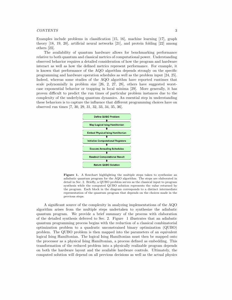
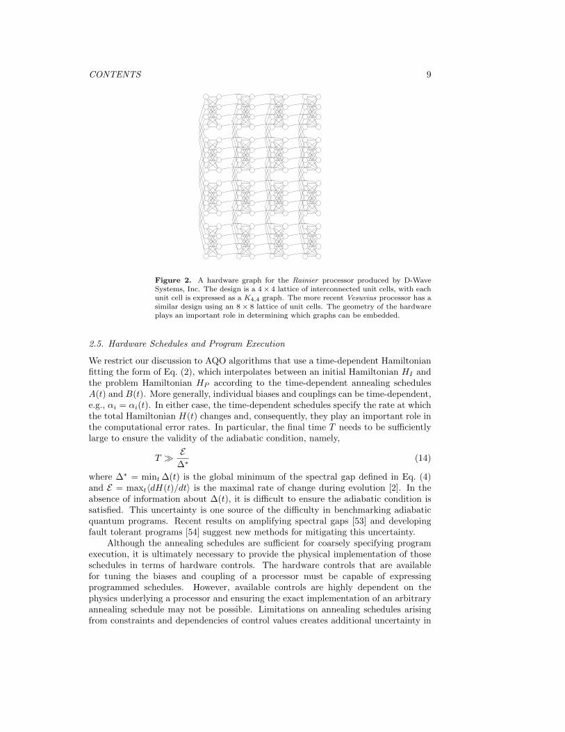
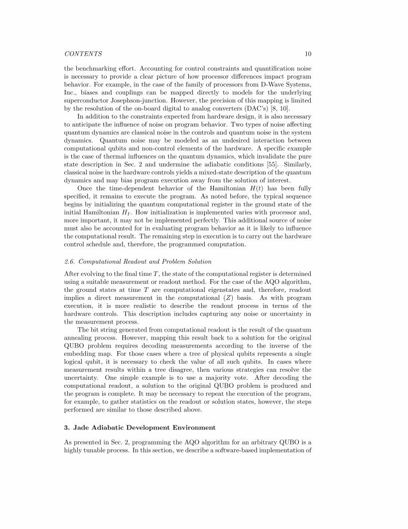
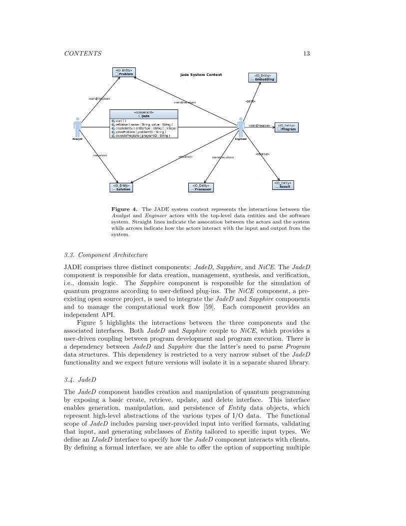
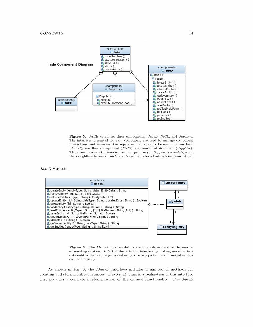
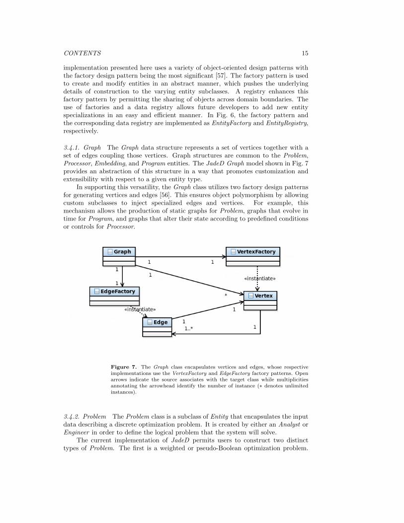
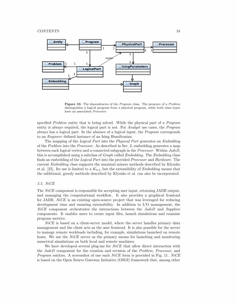
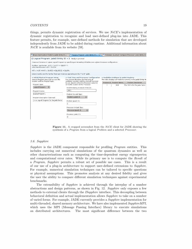
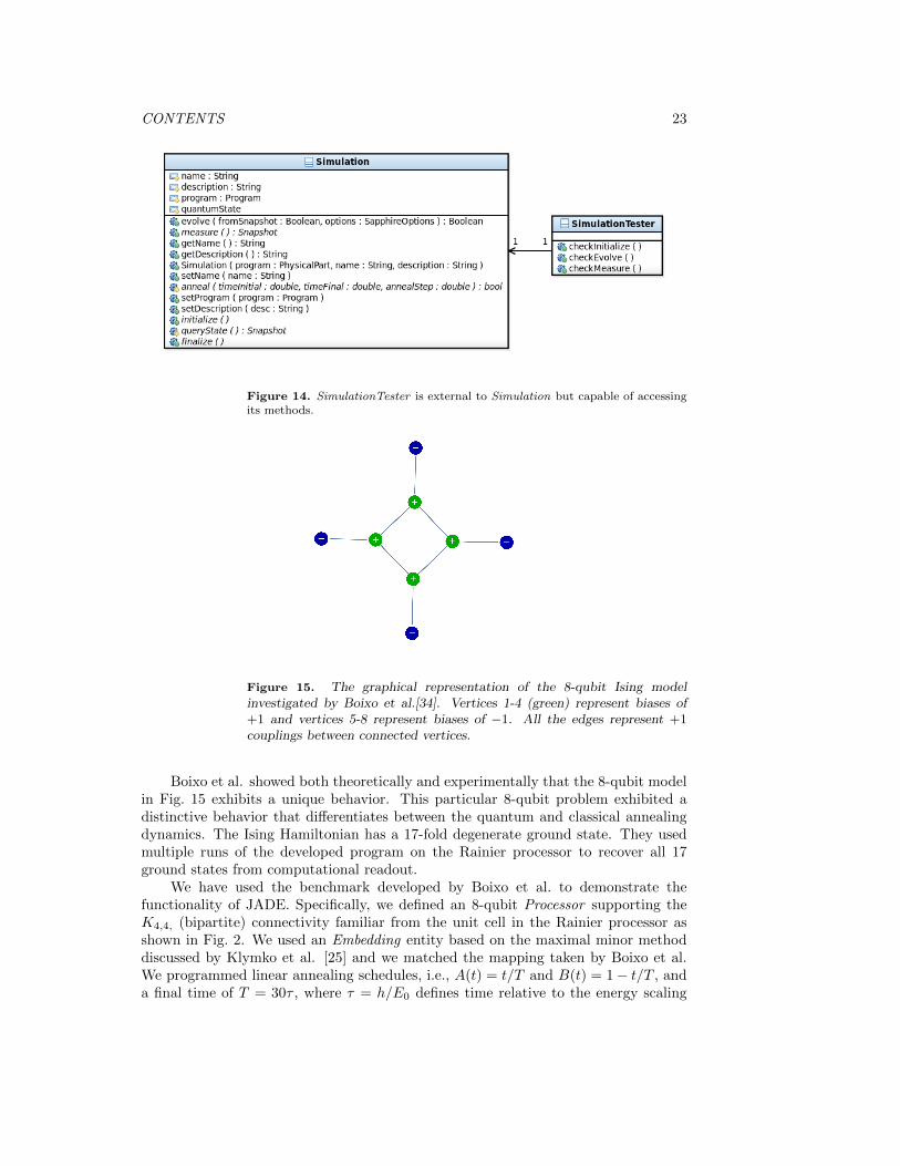
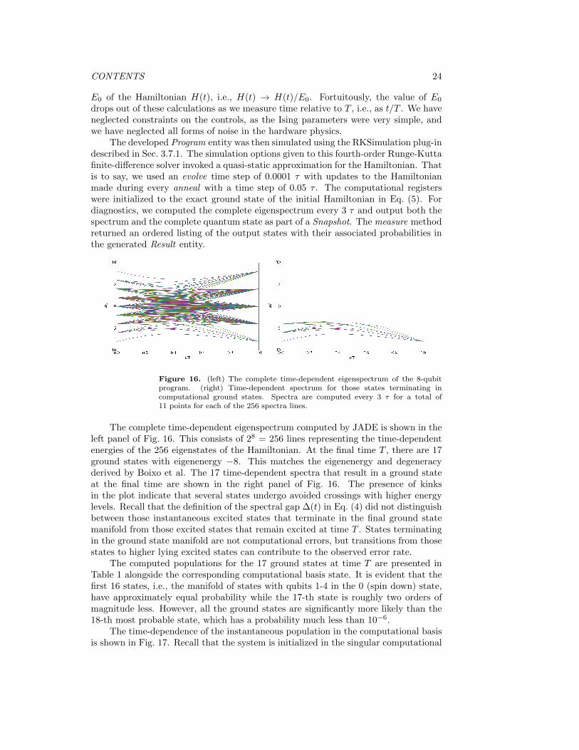
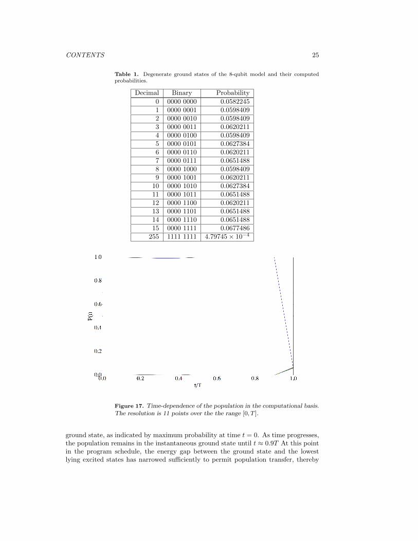