an integrated ecosystem model for coral reef management
TRANSCRIPT

An integrated ecosystem model for
coral reef management
where oceanography, ecology and socio-economics meet
Mariska Weijerman

Photo on front cover is Tumon Bay in Guam, photo NOAA

i
An integrated ecosystem model for
coral reef management
where oceanography, ecology and socio-
economics meet
Mariska Weijerman

ii
Thesis committee
Promotors
Prof. Dr. R. Leemans
Professor of the Environmental Systems Analysis Group
Wageningen University, Netherlands
Prof. Dr. W.M. Mooij
Professor of Aquatic Foodweb Ecology
Wageningen University, Netherlands
Co-promotors
Dr. E.A. Fulton,
Senior principal research scientists, Head of Ecosystem Modelling
Commonwealth Scientific and Industrial Research Organisation Oceans & Atmosphere,
Australia
Dr. R.E. Brainard
Division chief, Pacific Islands Fisheries Science Center, Coral Reef Ecosystem Division
National Oceanic and Atmospheric Administration, United States of America
Other members
Prof. Dr. Nick Polunin, University of Newcastle upon Tyne, UK
Prof. Dr. Tinka Murk, Wageningen University, Netherlands
Prof. Dr. Jack Middelburg, Utrecht University, Netherlands
Dr. Ronald Osinga, Wageningen University, Netherlands
This research was conducted under the auspices of the Graduate School for Socio-Economic
and Natural Sciences of the Environment (SENSE)

iii
An integrated ecosystem model for
coral reef management
where oceanography, ecology and socio-economics meet
Mariska Weijerman
Thesis
submitted in fulfillment of the requirements for the degree of doctor
at Wageningen University
by the authority of the Rector Magnificus
Prof. Dr Ir A.P.J. Mol,
in the presence of the
Thesis Committee appointed by the Academic Board
to be defended in public
on Wednesday 16 September 2015
at 11 a.m. in the Aula.

iv
Mariska Weijerman
An integrated ecosystem model for coral reef management
where oceanography, ecology and socio-economics meet,
289 pages.
PhD thesis, Wageningen University, Wageningen, NL (2015)
With references, with summary in English
ISBN 978-94-6257-430-4

v
Table of Contents
Chapter 1 General introduction .................................................................................................................... 2
1.1 Background .............................................................................................................................................................. 3
1.2 Step-wise approach .................................................................................................................................................. 5
1.3 Significance and novelty of thesis ........................................................................................................................... 9
1.4 Overall research objective and research questions ................................................................................................ 11
1.5 Outline thesis ......................................................................................................................................................... 12
Chapter 2 How models can support ecosystem-based management of coral reefs .................................... 16
2.1 Introduction ........................................................................................................................................................... 18
2.2 Categorization of three coral reef model types: Minimal, intermediate and complex ........................................... 21
2.3 Multiple model strategies in relation to coral reef management ............................................................................ 30
2.4 Concluding remarks ............................................................................................................................................... 33
Chapter 3 Coral reef ecosystems and performance indicators ................................................................... 35
3.1 Introduction ........................................................................................................................................................... 37
3.2 Methods ................................................................................................................................................................. 38
3.3 Results ................................................................................................................................................................... 45
3.4 Discussion .............................................................................................................................................................. 49
3.5 Conclusions ........................................................................................................................................................... 52
Chapter 4 Design and parametrization of a coral reef ecosystem model for Guam ................................... 54
4.1 Introduction ........................................................................................................................................................... 56
4.2 Guam ..................................................................................................................................................................... 59
4.3 Methods ................................................................................................................................................................. 65
4.4 Results ................................................................................................................................................................... 95
4.5 Discussion .............................................................................................................................................................. 96
Chapter 5 Coral reef-fish biomass trends based onshore-based creel surveys in Guam ............................ 99
5.1 Introduction ......................................................................................................................................................... 101
5.2 Methods ............................................................................................................................................................... 103
5.3 Results ................................................................................................................................................................. 109
5.4 Discussion ............................................................................................................................................................ 116
Chapter 6 Applying the Atlantis model framework to coral reef ecosystems ......................................... 119
6.1 Introduction ......................................................................................................................................................... 121
6.2 Methods ............................................................................................................................................................... 122
6.3 Results ................................................................................................................................................................. 128
6.4 Discussion ............................................................................................................................................................ 135
6.5 Concluding remarks ............................................................................................................................................. 137

vi
Chapter 7 Ecosystem modelling applied to coral reefs in support of ecosystem-based management ..... 139
7.1 Introduction ......................................................................................................................................................... 141
7.2 Methods ............................................................................................................................................................... 142
7.3. Results ................................................................................................................................................................ 150
7.4 Discussion ............................................................................................................................................................ 156
7.5 Conclusions ......................................................................................................................................................... 159
Chapter 8 Towards an Ecosystem-based approach of Guam’s coral reefs: the human dimension ........ .161
8.1 Background .......................................................................................................................................................... 163
8.2 Methods ............................................................................................................................................................... 166
8.3 Results ................................................................................................................................................................. 169
8.4 Discussion ............................................................................................................................................................ 172
8.5 Next steps ............................................................................................................................................................ 176
8.6 Conclusion ........................................................................................................................................................... 176
Chapter 9 Synthesis .................................................................................................................................. 178
9.1 Overview ............................................................................................................................................................. 179
9.2 Reflections on model development and its application ....................................................................................... 179
9.3 Complexity of coral reef modelling for MSE application ................................................................................... 181
9.4 Challenges and limitation of the model ............................................................................................................... 182
9.5 Research findings ................................................................................................................................................ 183
9.6 Conclusion ........................................................................................................................................................... 184
References ................................................................................................................................................. 187
Appendices ................................................................................................................................................ 211
Summary ................................................................................................................................................... 270
Acknowledgements ................................................................................................................................... 272
Publications ............................................................................................................................................... 273

1
School of jacks. Photo NOAA

2
Chapter 1
General introduction
3
1.1 Background
Human well-being is linked to natural resources and the increase in human population and
their activities leads to multiple users vying for the same resources. These uses can be of
monetary benefits, for example, commercial and recreational fisheries, oil and gas mining,
coastal development and aquaculture or of non-monetary benefits, such as cultural and
spiritual values, and of ecosystem services (Costanza et al. 1998). Humans have now affected
many of the earth’s ecosystems and their services (Birkeland 2004, Doney et al. 2012,
McCauley et al. 2015). These affected services include regulating services (e.g., the biogenic
structure of reefs mediating extreme weather and the recycling of nutrients and detoxification
of pollutants), provisioning services (e.g., food and medicines) and cultural services (e.g.,
cultural and spiritual values) upon which people and societies depend. Managing multiple
uses are challenges confronting resource managers responsible for maintaining sustainable
use of natural resources and preventing or mitigating the degradation of ecosystem services.
Coral reef ecosystems are especially vulnerable to climate change and worldwide a
third of reef-building coral cover is projected to be lost by 2050 (Carpenter et al. 2008,
Jackson 2008). Already live coral cover has declined since the seventies, with an estimated
decline of 20% worldwide (Wilkinson 2008), 40% in the Indian and southwest Pacific Ocean
(Bruno and Selig 2007), 50% in the Great Barrier Reef, Australia (De'ath et al. 2009), 70% in
the East Asia Seas (Yap and Gomez 1985) and 50% in the Caribbean (Jackson et al. 2014).
These declines are attributed to land-based sources of pollution, including sedimentation and
eutrophication, and destructive fishing practices, overfishing and mortality events related to
elevated temperatures, with most noteworthy being the global mass ‘bleaching’ events in
1998 and 2005 (bleaching is the expulsion of the symbiotic microscopic algae in the coral
tissue). With the decline in coral cover the species they harbor are likely to decline as well
(Jones et al. 2004, Munday 2004b). The main objective of this thesis is to develop a model to
quantify the effects of watershed and fishery management on ecosystem services in order to
evaluate the economic and ecological tradeoffs of alternative management policies against a
backdrop of climate change.
Vulnerability of coral reef ecosystems to natural and human-induced disturbances is a
function of (1) exposure to present and future climate states and human activities; (2)
sensitivity or resistance (species can avoid or adapt to exposure depending on genes, local
environmental variability and surrounding environmental changes); and (3) the capacity to
recover (which depends on the availability of resources that enhance resilience, such as
ecological factors, species and functional diversity, spatial factors, reproduction and
connectivity, and shifting geographic ranges [reviewed in Brainard et al. 2011]). Local
drivers and changing climate threaten the ecosystem functions and services that coral reef
ecosystems provide. Ocean warming (e.g., Donner et al. 2005, Donner 2009), ocean
acidification (e.g., Guinotte et al. 2003) and their synergistic effects (Harvey et al. 2013) have
been ranked as the top proximate threats in recent reviews (Brainard et al. 2011, Burke et al.
2011). Disease, often associated with bleaching events and local human impacts, was ranked
as the next most important threat in those reviews. Some researchers, however, have
identified grounds for optimism: vulnerability assessments of corals and coral reef fishes to
ocean warming and fishing indicated that reduced fishing may enhance key ecosystem

4
processes and this likely increases a reef’s capacity to recover (e.g., McClanahan et al. 2014).
Other studies also indicated that local management regulations in reducing sedimentation,
nutrient input and fishing can mitigate the effects of the imminent global threats (Carilli et al.
2009, Hughes et al. 2010, Graham et al. 2011b, Kennedy et al. 2013).
Traditionally, fishing regulations were based on single species management but
recently there has been a fundamental shift towards ecosystem-based management (EBM) or
ecosystem-based fisheries management (EBFM) with research and management coming to
focus on the advantages of EBM (Hilborn 2011), including the development of EBM
indicators (Fulton et al. 2005, Coll et al. 2010) and studies on cumulative effects on
ecosystems of various disturbances (Brown et al. 2010, Griffith et al. 2012). Although the
concept of EBM was originally introduced in 1873 by Spencer Baird (1873), EBM is only
now the dominant approach advocated by researchers (Pikitch et al. 2004, Levin et al. 2009)
and increasingly mandated by national fisheries policies and international agreements, for
example, the U.S. National Ocean Policy 2010 (Executive Order 13547 2010) and the
European Common Fisheries Policy 2014 (http://ec.europa.eu/fisheries/cfp/index_nl.htm).
However, implementing EBM is not straightforward, due to the many, frequently conflicting,
objectives of the various stakeholders (Link 2002) and the lack of suitable operational tools
(Arkema et al. 2006).
EBM can be supported by ecosystem models that can help disentangle the effects of
consumer-resource dynamics, habitat and climate factors (Guerry et al. 2012, Samhouri et al.
2013). Models have thus become important tools for gaining insights in to system changes
due to human (e.g., fishing) or environmental (e.g., hurricanes) disturbances, to further
develop theories of system function and interconnection, to identify tipping points, to assess
trends by indicators and to point out research gaps (Mumby et al. 2007a, Fulton et al. 2011b,
Ainsworth and Mumby 2014). Additionally, ecosystem models can simulate policy scenarios
and evaluate the tradeoffs among stakeholders’ objectives (Smith et al. 2007, Fulton et al.
2014). For example, real-world experimentation of large-scale fishery regulations is not
generally feasible but tradeoffs can be evaluated using ecosystem models. Multi-species or
ecosystem models can also complement single-species stock-assessment models and provide
a more integrated framework for system-wide decision-making by focusing on emergent
properties at the community and ecosystem levels (Fogarty 2013).
For the judicious use of ecosystems models as a management tool we need to ensure
that they capture the combination of the effects of external drivers and internal feedbacks that
shape these systems and their resilience under environmental change. On coral reefs, and on
other systems, local drivers often influence or reinforce feedback mechanisms (Nyström et al.
2012) and other interactions between functional species groups. Examples include the shift in
the energy balance from macrobes to microbes due to fishing, pollution and/or coastal
development (McDole et al. 2012); a disruption in alga-coral-grazer dynamics due to a
reduction in grazers and/or an increase in nutrients causing a shift from coral-dominated reefs
to algal-dominated reefs (Mumby 2006, Mumby and Steneck 2008); trophic cascades due to a
take of apex predators (Williams et al. 2008); a loss of fish abundance due to fishing
(Williams et al. 2015); and a decline in fish diversity and abundance due to a decline in
structural complexity resulting from a loss in coral cover (DeMartini et al. 2013, Graham and
5
Nash 2013). The capacity of organisms and natural systems to ‘bounce back’ can be degraded
by sequential, chronic and multiple disturbances, physiological stress and general
environmental deterioration (Nyström et al. 2000) and by the reduction of large and diverse
herbivorous fish populations (Pandolfi et al. 2003, Bellwood et al. 2006). These dynamics
and their relationships need to be included correctly in a coral reef ecosystem model to
ascertain that model simulations are representative of the real system so that model
projections are accurate and reliable.
The deterministic, spatially-explicit coral reef model, developed in this thesis, is an
integrated framework that focuses at the emergent properties at the community and
ecosystem level and can be used for system-wide decision-making and management strategy
evaluation (MSE). To give it this capacity the inclusion of the myriad coral reef ecosystem
relationships was needed. The identity of these relationships was established from simulation
outcomes of other coral reef models and empirical field studies on reef systems. The Atlantis
ecosystem modelling framework, developed for temperate fisheries systems, provided a
flexible platform for the coding of tropical reef functionality, as it already specifically
supported ecosystem scale MSE (Plagányi 2007). Atlantis’ modular framework allows
parameterization to be as detailed per module as desired by the developer, and Atlantis
incorporates dynamic two-way interactions between oceanographic, ecological, biochemical
and socio-economic processes. In this thesis, I explain my step-wise approach to the
development and application of the Atlantis Coral Reef Ecosystem model (Guam Atlantis)
with a case study of the reefs around Guam in the western tropical Pacific Ocean.
1.2 Step-wise approach
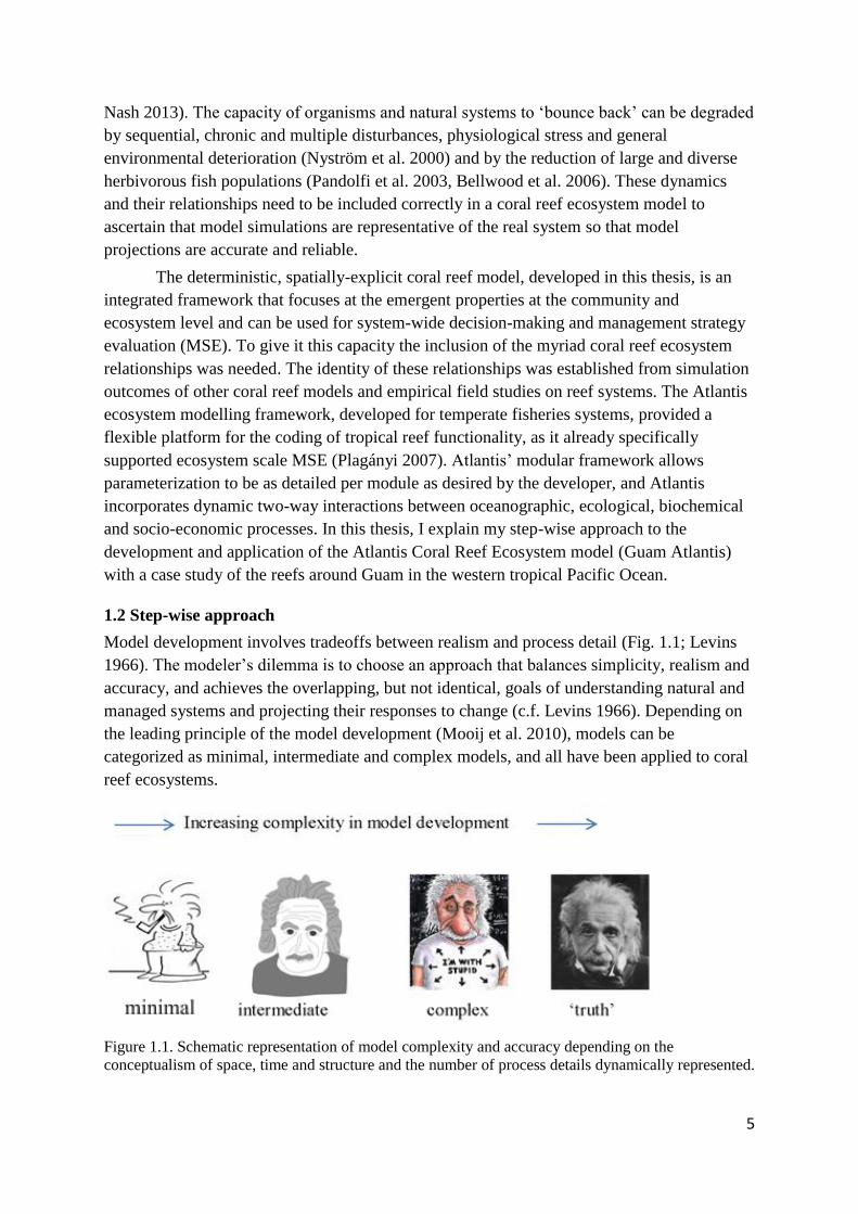
Model development involves tradeoffs between realism and process detail (Fig. 1.1; Levins
1966). The modeler’s dilemma is to choose an approach that balances simplicity, realism and
accuracy, and achieves the overlapping, but not identical, goals of understanding natural and
managed systems and projecting their responses to change (c.f. Levins 1966). Depending on
the leading principle of the model development (Mooij et al. 2010), models can be
categorized as minimal, intermediate and complex models, and all have been applied to coral
reef ecosystems.
Figure 1.1. Schematic representation of model complexity and accuracy depending on the
conceptualism of space, time and structure and the number of process details dynamically represented.

6
An ecosystem model can be seen as an abstract representation of a set of hypotheses
that are either tested with empirical studies, theories or with minimal or intermediate models.
The integration of system dynamics can be achieved through complementary use of models
or through integrated models that combine many aspects of the system in one framework
(Butterworth and Plaganyi 2004). Coral reef ecosystem models to date have generally
focused on one or two external factors, such as, climate, nutrient and sediment inputs and
fisheries (McClanahan 1995, Arias-González et al. 2004, Ainsworth et al. 2008b, Buddemeier
et al. 2008, Riegl and Purkis 2009, Anthony et al. 2011b, Blackwood et al. 2011). Internal
feedbacks have also been studied with coral reef models to provide insights into how these
systems respond (e.g., linearly or non-linearly) to external factors and whether or not changes
in system state lead to regime shifts or alternative stable states (Bellwood et al. 2004, Mumby
2006, Mumby et al. 2007a, Yñiguez et al. 2008, Renken and Mumby 2009, Tam and Ang
2012, Żychaluk et al. 2012).
For a full understanding, models need to capture how species- and ecosystem-level
responses interact, as well as representing the link between species- and ecosystem-level
processes accurately. Additionally, when attempting to understand the effects of human
activities, these models need to capture the two-way dynamics between human use and
ecological impacts and should be coupled with socio-economic models. Few models have
included the various human activities that alter the coral reef dynamics and simultaneously
the socioeconomic context in which they occur (Kramer 2007, Tsehaye and Nagelkerke 2008,
Fung 2009, Melbourne-Thomas et al. 2011b). With the new insights provided by empirical
studies and model results, a coral reef ecosystem model can now dynamically integrate the
underlying biological processes that confer resilience and sustainability to reefs, with
biochemical and hydrological dynamics and place those in the context of human activities.
To choose the appropriate model type and for proper model development, the
objectives should be clear and upfront and stakeholders should be involved. I followed the
guidelines for Integrated Ecosystem Assessments (Levin et al. 2009) for my ecosystem model
development. The steps I took are presented in the following chapters in my thesis and
include:
1. Scoping. In this step the specific ecosystem objectives and threats were identified. During
a workshop that I organized together with the NOAA Pacific Islands Fisheries Science
Center and the Pacific Islands Regional Office (PIRO), invited speakers presented the
current status of Guam reefs, the main threats to those reefs, including a focus on the
potential effects of the proposed military build-up in Guam. With that current context in
place, I explained how ecosystem models in general, and the Atlantis model in particular,
could serve as a decision-support tool in visualizing coral reef trajectories under
alternative policy scenarios. Workshop participants discussed the overall goals of
ecosystem metrics, identified ecological and economic indicators, and management
strategies to assist resource managers in making educated decisions, based on evaluation
of the economic and ecological tradeoffs highlighted by model simulations (Weijerman
and Brown 2013 and unpublished results of meetings in July 2014).

7
2. Indicator Development. Ecosystem indicators that were identified during the workshop
in 2012 (Weijerman and Brown 2013), are tested with an ECOPATH model (Christensen
and Pauly 1992, Christensen et al., 2008). These indicators provide the basis for the
assessment of status and trends in ecosystem state. Some of the selected indicators
represent the abundance of key species while others serve as proxies for ecosystem
attributes (e.g., maintenance of critical service functions, system maturity).
3. Risk Analysis. Having identified the leading principle for model development and the
indicators, I evaluated the risk to these indicators posed by human activities and natural
processes using a complex, end-to-end modelling framework, Atlantis
(http://atlantis.cmar.csiro.au/). First I designed and parameterized the Atlantis model and
then included key coral reef dynamics. From the literature, I identified the main drivers
influencing the sustainability of ecosystem services (Brainard et al. 2011, Principe et al.
2012) (Table 1.1) and developed ways to incorporate the underlying response
mechanisms, derived from published empirical relationships or from other coral reef
models, into the Guam Atlantis model.
A common maxim of model development is that ‘less is more’ (Levins 1966), i.e.,
one should only incorporate the key mechanisms and functional groups, balancing
accuracy, complexity and realism of various dimensions, such as time, space, trophic
components, process details, human activities, boundary conditions and forcings. Whole-
of-system or end-to-end models are data intensive with high spatial and functional
complexity compared to minimal or intermediate models but they can be robust when
reasonable limits are set on their complexity (Fulton et al. 2003a, Fulton et al. 2003b,
2004c, Mitra and Davis 2010), the relevant biological groups and functions are
considered and enough detail is incorporated to make accurate predictions (Travers et al.
2007).
Table 1.1. Key drivers, pressures (proximate threats) and affected coral reef ecosystem variables.
Drivers Pressures Ecosystem Indicators
changing climate ocean warming: elevated
water temperatures
coral growth & mortality, coral
recruitment, and benthic species
composition
ocean acidification:
increasing atmospheric
CO2 concentrations and
oceanic uptake
growth of corals and other calcifying
species, benthic species composition,
coral recruits; and survival rate of
juveniles,
change in land
use
sedimentation; non-point
sources of pollution;
nutrients; and disease
coral growth, cover, species composition,
recruitment; turbidity; and algal cover
fishing activity excessive fishing coral and algal cover; fish biomass,
abundance, size distribution and species
composition; complexity; income/food
for fisherman; and added value from
fishing expenditures

8
After identifying the key dynamics and researching how to incorporate their
relationship from empirical data and coral reef model simulations (see Chapter 6), the
Atlantis code was modified to represent (a) coral growth in three dimensions; (b) coral-
algal competition (e.g., space competition and macro-algal overgrowth); (c) negative
effects of sediments on coral growth; (d) the positive feedback between the structural
complexity of corals and fish (i.e., corals provide shelter to small and juveniles fishes
while herbivorous fishes maintain coral reef algal assemblages in cropped states
facilitating coral recruitment); (e) the ‘bleaching’ phenomenon, in which corals expel a
portion of their symbionts (which causes the corals to lose color and appear ‘bleached’)
when temperatures rise above a threshold; such bleaching event can results in total or
partial mortality, with associated scope for short-term recovery; and (f) the negative
effects of a decline in pH (i.e., ‘acidification’) on reef organisms including corals.
Criteria used for testing the validity of the model and to verify model outcomes
were based on guidelines for Atlantis model development (Horne et al. 2010, Link et al.
2010, Ainsworth et al. 2011, Fulton et al. 2014) and include: 1) Predicted biomass
matches observations or are plausible based on information from domain experts. In this
case for many benthic groups this defaults to staying within a factor of two of initial
conditions. For fish groups we expected predicted biomass (with no fishing or other
drivers) to approximate those in marine reserves in Guam or from the unpopulated
Northern Mariana Islands; 2) Weight-at-age stays stable and abundance of size classes
decreases with increasing size classes (few large organisms and many small ones); and 3)
Reproduced catch data has a plausible trajectory and magnitude of historical change
without pushing any modeled group to extinction. Ecosystem relationships related to
disturbances were validated by comparing model outcomes with empirical data and
published literature. Based on the compliance with all three criteria and agreements
between model outcome and expectations, I concluded that the Guam Atlantis model was
stable with plausible biomass trajectories. With this model I then quantitatively compared
the trajectories of the chosen indicators while simulating a range of anthropogenic
drivers—land-based sources of pollution, fishing and climate change—separately and
simultaneously.
4. Management Strategy Evaluation. Complex end-to-end models cannot be tractable
evaluated using standard validation and sensitivity analyses (Stow et al. 2009).
Consequently, this makes them unsuitable for tactical management, such as setting catch
quotas or identify areas for protection from fishing. However, when MSE is justified,
these end-to-end models are important strategic management tools to project how reefs
will respond to the current global disturbances under alternative local management
strategies. I will use the MSE approach to evaluate the potential of different management
strategies to influence the status of natural and economic indicators (Fig. 1.2). By
coupling this model to a Bayesian Network model framework, I was also able to identify
the cultural and social-economic tradeoffs of the alternative management policies.

9
Figure 1.2. Example of the use of Atlantis for management strategy evaluation for the Gulf of
California (as of Ainsworth et al. 2012). Various alternative management policies were simulated
independently and all together (i.e., the full enforcement top right) to visualize and quantify the
effects on the indicators.
1.3 Significance and novelty of thesis
In a wider context, this thesis forms part of the modelling work of the Atlantis ecosystem
modelling community. Atlantis was developed by Dr. Elizabeth (Beth) Fulton
(Commonwealth Scientific and Industrial Research Organisation) in 2001 and has since been
applied to a range of temperate marine ecosystems in Australia, the US, South Africa and
Europe, with tropical and polar examples under development (Fulton et al. 2011b). As EBM
has become more prominent in national policies, so has the need for tools, such as ecosystem
models, to inform EBM. Whole-of-system or end-to-end models, such as Atlantis, model the
full suite of marine ecosystem dynamics, uses, management and feedbacks and synergies.
Atlantis was designed as one of the very few modelling platforms that can handle “sunlight to
fish markets and everything in between,”
(http://atlantis.cmar.csiro.au/www/en/atlantis/Atlantis-Summit.html) particularly linking
biophysical Regional Ocean Model Simulations (ROMS) to ecology with anthropogenic
modules to interface with the various socio-economic facets of a marine ecosystem. The
uniqueness of Atlantis is that it is multi-sector, modular, has multiple functional forms a user
can choose, and it is designed specifically to address system-level management strategy
evaluation. However, to maintain its usefulness Atlantis needs on-going development,
refinement, testing and evaluation of the myriad modular approaches it provides in a variety
of ecosystems.

10
All fully implemented and published applications of Atlantis to date have focused on
temperate systems whereas Guam Atlantis, the model in this study, focuses on tropical coral
reef ecosystems. Currently the University of South Florida is developing an Atlantis model
for the Gulf of Mexico (including corals) and CSIRO is developing models for the Great
Barrier Reef and Gladstone harbor (also including corals). The Guam Atlantis model differs
from these models in its size of the spatial domain (e.g., 100 km2 for Guam Atlantis
compared to 1.6 million km2 for the Gulf of Mexico). The Guam Atlantis model is likely
more sensitive to benthic community processes and the dynamics that influence them.
Parameterization of Guam Atlantis can aid these other more broad-scale models with details
where needed.
Another novelty is the coupling of a Bayesian Network Model framework detailing
the motivation and fishing activity of Guam’s fisherman to Guam Atlantis. Since coral reef
fisheries are considered to be more recreational than commercial in Guam (e.g., Van
Beukering et al. 2007), economic ‘rules’ that govern the decision to go fishing for
commercial reasons (which is the case when large areas are of concern) do not apply. Instead,
the motivation to go fishing is driven by a desire to fish for fun, to put dinner on the table or
for cultural reasons (Allen and Bartram 2008). Hence, the economic module of Atlantis,
which was initially developed to represent the commercial fishery, does not fit well with the
motivation for fisherman in Guam. A similar approach has also been used for a recreational
lobster fishery by indigenous fisherman in the Torres Strait (van Putten et al. 2013), but has
not previously been coupled to any Atlantis model. Marine tourism is of major economic
importance in Guam (Van Beukering et al. 2007). I, therefore, also developed a Bayesian
Network Model framework for dive tourism, which is coupled with the fishery motivation
model to form the full Guam Atlantis ecosystem model (Chapter 8).
My thesis research also innovatively addresses the myriad threats that coral reefs face
simultaneously. Many coral reef models have been developed, but only a few dynamically
incorporate the oceanographic, ecological and biogeochemical processes, and none
specifically include the spatial heterogeneity of a reef with a high-resolution daily time-step.
Atlantis is generic enough in its dynamic processes to apply to other Pacific islands where
there is sufficient data for quantifying the initial conditions (e.g., spatial model based on
homogenous areas, biomass of all functional groups, spatial distribution of groups, life-
history parameters if the biological communities differ greatly from the ones in Guam). The
model-generated results aid in identifying the ecological and economic ‘pros and cons’ of
alternative management policies, taking into account the current and future climate change
threats. Resource managers can make more informed decisions based on those results.
This thesis investigates quantitatively the synergy of different drivers and the form of
the relationships. First, the relationship (i.e., feedbacks, synergies and tradeoffs) between
fishing, eutrophication and sedimentation (local drivers) was investigated. Secondly, the
relationship between ocean acidification and ocean warming was investigated. And lastly, the
interaction between both the local and global drivers was investigated. Simulations were
performed with the reef system being exposed to one driver, than two and ultimately all three.
Results showed only slight synergies but did suggest that fishing now (1985–2015) and
climate change in the future (1985–2050) greatly impacted ecosystem metrics.

11
The thesis also advances coral reef modelling development in general and in
particular for the Atlantis model community. The model described in this thesis also differs in
its complexity from the many coral reef ecosystem models developed earlier. The model aims
to include all functional species groups relevant in coral reef dynamics. Other studies have
shown the importance of including the detrital pathways, which are very prominent in coral
reefs (Paves and Gonzalez 2008) but have mostly been omitted in ecosystem models of reefs
with the exception of the CAFFEE model (Ruiz Sebastián and McClanahan 2013). Bellwood
et al. (2004) explained the importance of including the various groups of herbivores and their
functional roles to properly account for changes in reef resilience and, although most coral
reef models include herbivores, they are often lumped into one or a few functional groups
whereas I group them by their functional role as grazers (preventing turf algae from growing
into macroalgae), browsers (cropping down macro-algae), scrapers (scraping algae of the
substrate opening up space for coral recruits), excavators (important bio-eroders and opening
up substrate) and detritivores (recycling sediments). Moreover while structural complexity is
recognized as greatly influencing fish diversity and abundance, it has only recently been
given more prominence in coral reef models (Bozec et al. 2013, Bozec et al. 2014) and had
not previously been combined with other disturbances or key reef dynamics in reef models.
Similarly, the trophic role of apex predators had not generally been properly included into
coral reef models. I included both (the influence of structural complexity via a derived
relationship between complexity and prey vulnerability and trophic interactions), along with
the main human-induced drivers to the reef. By representing this combination of socio-
ecological processes the model can provide a more complete perspective on future reef
trajectories.
1.4 Overall research objective and research questions
The overall research objective of this thesis is to quantify the effects of watershed and fishery
management on ecosystem services using an ecosystem model in order to evaluate the
economic and ecological tradeoffs of alternative management policies against a backdrop of
climate change. To address this overall objective I explored the following research questions:
● What are the main goals of and differences between minimal, intermediate and
complex models of coral reef ecosystems? Which approach(es) or combination of
approaches obtain the most clarity and predictive capabilities if used in a management
strategy evaluation framework?
● How does fishing affect ecosystems states? What are the most reliable indicators of
fishing on coral reef ecosystem structure and function?
● Can local management strategies mitigate the impacts of climate change (ocean
warming and acidification) on coral reef ecosystems? What is the effect size on
performance metrics of key drivers to reefs when acting individually and
concurrently?
● What are socio-economic and ecological tradeoffs of the existing rules and
regulations governing reef fishery and conservation compared to the selected
alternatives?

12
● What motivates Guam’s fishers to go fishing for reef fish and what determines the
level of tourist participation in diving on coral reefs in Guam? How does the coral
reef ecosystem state affect these participation rates and what are the effects of
changes in these activities on the ecosystem?
1.5 Outline thesis
The step-wise approach (Section 1.2) and the research questions (Section 1.4) are combined and
addressed in the various chapters in my thesis as indicated in Figure 1.3. By answering the
research questions, parts of the puzzle are resolved, until at the end I can piece them all together
and so achieve the general objective. This thesis consists of nine chapters including this
introduction and a synthesis as the final chapter (Fig. 1.3). Chapters 2–8 are either already
published or in various stages of the publication process. All chapters are written in
collaboration with other scientists and I am the first author in all of them. A brief summary of
each of the chapters follows.
Chapters: 2 3 4, 5, 6 7 and 8
Figure 1.3. Schematic representation of the steps taken to model development and implementation and
how they are linked with various research questions (RQ: for full description see Section 1.4)
addressed in the various chapters of this thesis and which, when pieced together, provide insight to the
overall objective (figure adapted from Fulton et al. 2011a).

13
In Chapter 2, my co-authors and I reviewed the roles of three model types—classified
based on their complexity as minimal, intermediate and complex models—in supporting
sustainable coral reef ecosystem services. We highlighted the need to invest time in
appreciating the identity and potential of each of the three model types in its own right and in
concert. Minimal coral reef models are crucial to our understanding of ecosystem feedback
loops and their response curves (e.g., linear, non-linear, modal). Understanding the drivers of
change in a system’s state will improve scope for effective management responses, reversing
or preventing change. Intermediate models can assist managers with projections of ecosystem
responses and indirect outcomes through the inclusion of the full spectra of trophic groups.
These models can be used to answer many questions as they also include various
environmental or anthropogenic forcings. For managers all-encompassing complex models
may be the most informative decision-support tool for evaluating the economic and
ecological tradeoffs of various management scenarios. These models are the ones that include
all major dimensions (i.e., spatial, temporal, taxonomic, nutrient, human activities) in their
simulations and, therefore, incorporate the often synergistic effects of various dynamic
mechanisms and responses that may be omitted by minimal or intermediate models which
sacrifice on these dimensions in return for transparency and ease of construction.
In Chapter 3, my co-authors and I assessed suitability of potential indicators of fishing
pressure to coral reef ecosystem state. Despite the increase in number of modelling studies in
coral reef areas, adequate information on appropriate indicators to quantify changes in these
systems is still lacking. This chapter focuses on the quantitative description of characteristics
of ecosystem attributes of three coral reef systems in Hawai`i along a fishing pressure
gradient and identifies the most reliable indicators of ecosystem structure and function of
coral reefs to support ecosystem-based fishery management. We also considered and
compared our models with three other ecosystem models developed for Hawai`i: one
concentrating on the role of herbivores in reef resilience at Kaloko-Honokohau National
Historical Park; one characterizing the reef ecosystem structure along the Kona coast of
Hawai`i; and the third one estimating the carrying capacity of monk seals at French Frigate
Shoals in the Northwestern Hawaiian Islands. In contrast to those other studies, which focus
on energy flows, our model and study uses the Ecopath model to assess key indicators related
to fishing pressures.
Chapter 4 describes the design and parameterization of the Atlantis ecological module
to make it suitable for coral reef ecosystems around Guam. This work, therefore, builds on
the functionalities and deterministic relationships included in the base Atlantis model
framework and already validated in Atlantis-related papers (e.g., Fulton et al. 2011b,
Ainsworth et al. 2012, Griffith et al. 2012, Kaplan et al. 2012, Fulton et al. 2014). We give an
overview of the separation of the species inhabiting a coral reef into functional groups and
explain the data needs and sources of the various parameters used in this model. At this stage,
coral reef dynamics and an oceanographic module were not yet implemented (see instead
Chapter 6).
Chapter 5 describes an assessment of historic trends in the biomass of coral reef fish
species around Guam from fishery-dependent and independent data. A core goal was to use
catch time-series data to derive a reef-fish biomass time series that could be used to (later)

14
test Atlantis model outputs. Although various studies have indicated that reef-fish stocks have
declined around Guam, robust long-term time series data, based on actual survey data, are
lacking. In this chapter, we modified an approach used to estimate time series of fish stocks
based on single-species fishery data (Haddon 2010) and applied it to the multi-gear, multi-
species inshore reef-fish fisheries in Guam.
In Chapter 6, my co-authors and I assess the effect size of individual drivers (climate
change, land-based sources of pollution and fishing) and concurrent effect size of these
drivers on selected ecosystem metrics. We also assess the impact of local management on
coral biomass trajectories under present climate change predictions. In Appendix F
accompanying this chapter, we detail the modifications made to the Guam Atlantis ecosystem
model developed under Chapter 4, through the inclusion of code for the relationships of key
coral reef dynamics, with a particular focus on incorporating climate change impacts. This
appendix also includes validation of the new code.
Chapter 7 describes the application of ecosystem modelling as a tool for exploring
ecosystem level effects of changing environmental and management conditions. Policy
scenarios identified by the local and federal resource managers in Guam were simulated with
the Guam Atlantis model. Although Atlantis’ applicability and suitability is limited for
tactical management decisions (e.g., setting catch limits), it has value as a simulation
technique to give insight in the ecosystem effects of alternative management approaches and
to compare economic and ecological tradeoffs of each approach. Applying Atlantis to assess
management options for coral reef ecosystems is a novel application.
Chapter 8 takes the results of Chapter 7 and combines them with socio-economic
human behavior models to get insights into the socio-economic tradeoffs of the identified
scenarios.
In Chapter 9 I reflect on the model development and discuss the challenges and
limitations of the modelling approach and present a synthesis of the main findings and
conclusions.

15

16
Chapter 2
How models can support ecosystem-
based management of coral reefs
Weijerman, M, EA Fulton, ABG Janssen, JJ Kuiper, R Leemans, BJ Robson, IA van de
Leemput, WM Mooij. 2015. How models can support ecosystem-based management of coral
reefs. Prog. in Oceanography, online.

17
Despite the importance of coral reef ecosystems to the social and
economic welfare of coastal communities, the condition of these
ecosystems have generally degraded over the past decades. With an
increased knowledge of coral reef ecosystem processes and a rise in
computer power, dynamic models are useful tools in assessing the
synergistic effects of local and global stressors on ecosystem functions.
We review representative approaches for dynamically modelling coral
reef ecosystems and categorize them as minimal, intermediate and
complex models. The categorization was based on the leading principle
for model development and their level of realism and process detail. This
review aims to improve the knowledge of concurrent approaches in coral
reef ecosystem modelling and highlights the importance of choosing an
appropriate approach based on the type of question(s) to be answered. We
contend that minimal and intermediate models are generally valuable
tools to assess the response of key states to main stressors and, hence,
contribute to understanding ecological surprises. As has been shown in
freshwater resources management, insight into these conceptual relations
profoundly influences how natural resource managers perceive their
systems and how they manage ecosystem recovery. We argue that adaptive
resource management requires integrated thinking and decision support,
which demands a diversity of modelling approaches. Integration can be
achieved through complimentary use of models or through integrated
models that systemically combine all relevant aspects in one model. Such
whole-of-system models can be useful tools for quantitatively evaluating
scenarios. These models allow an assessment of the interactive effects of
multiple stressors on various, potentially conflicting, management
objectives. All models simplify reality and, as such, have their weaknesses.
While minimal models lack multidimensionality, system models are likely
difficult to interpret as they require many efforts to decipher the numerous
interactions and feedback loops. Given the breadth of questions to be
tackled when dealing with coral reefs, the best practice approach uses
multiple model types and thus benefits from the strength of these different
models.
18
2.1 Introduction
Coral reefs are extremely important as habitats for a range of marine species, natural buffers
to severe wave actions and sites for recreation and cultural practices. Additionally, they
contribute to the national economy of countries with coral reef ecosystems. The economic
annual net benefit of the world’s coral reefs are estimated at US$29.8 billion from fisheries,
tourism, coastal protection and biodiversity (Cesar et al. 2003). Moreover, coral reefs are
important to the social and economic welfare of tropical coastal communities adjacent to
reefs (Moberg and Folke 1999). Coral-reef related tourism and recreation account for US$9.6
billion globally and have also shown to be important contributors to the economy of Pacific
islands (Cesar et al. 2003, Van Beukering et al. 2007). However, the functioning of coral reef
ecosystems and their biodiversity is deteriorating around the world (Hoegh-Guldberg et al.
2007). In recent reviews on the extinction risks of corals, the most important global threats to
the survival of corals and coral reefs were human-induced ocean warming and ocean
acidification (Brainard et al. 2011, Burke et al. 2011). While local governments are limited in
their capacity to reduce greenhouse gas emissions worldwide and so reduce the on-going
ocean warming and acidification, they can play a pivotal role in enhancing the corals’
capability to recover from impacts of these global threats by reducing additional local
stressors caused by land-based sources of pollution and fishing (Carilli et al. 2009, Hughes et
al. 2010, Kennedy et al. 2013, McClanahan et al. 2014).
The capacity of coral reef organisms and natural systems to ‘bounce back’ from
disturbances can be degraded by sequential, chronic and multiple disturbance events,
physiological stress and general environmental deterioration (Nyström et al. 2000), and
through the reduction of large and diverse herbivorous fish populations (Pandolfi et al. 2003,
Bellwood et al. 2006). These local stressors affect the coral-macroalgal dynamics and early
life history development and survival of corals (Baskett et al. 2009b, Gilmour et al. 2013),
but these stressors can be mitigated by proper management (Mumby et al. 2007b, Micheli et
al. 2012, Graham et al. 2013). Ecosystem models can help managers in system understanding
and in visualizing projections of realistic future scenarios to enable decision making (Evans
et al. 2013). As has been shown in the management of freshwater resources, insight in the
conceptual relations between key states and their response to stressors can have profound
impacts on the way natural resource managers think about their systems and the options they
have for ecosystem recovery (Carpenter et al. 1999).
Large-scale regime or phase-shifts have been identified in pelagic systems (Hare and
Mantua 2000, Weijerman et al. 2005) and on coral reefs (Hughes 1994) and have influenced
a new understanding in ecosystem dynamics that includes multiple-equilibria, nonlinearity
and threshold effects (Nyström et al. 2000, Mumby et al. 2007a). The theory of alternative
stable states implies, for example, that a stressed reef could not only fail to recover after a
disturbance, but could shift into a new alternative stable state due to destabilizing feedbacks,
such as a change in abiotic or biotic conditions (Mumby 2006, Mumby et al. 2013b). As a
result, reversing undesirable states has become difficult for managers (Nyström et al. 2012,
Hughes et al. 2013), even when stressors are being lowered (a phenomenon also known as
hysteresis [Scheffer et al. 2001]).
19
The complexity of coral reef ecosystems with their myriad processes acting across a
broad range of spatial (e.g., larval connectivity versus benthic community interactions) and
temporal (e.g., turnover time of plankton versus maturity of sea turtles) scales makes
modelling coral reef ecosystems for predictive assessments very challenging. The modeler’s
dilemma is to choose an approach that juggles simplicity, realism and accuracy, and reaches
the overlapping but not identical goals of understanding natural systems and projecting their
responses to change (Levins 1966).
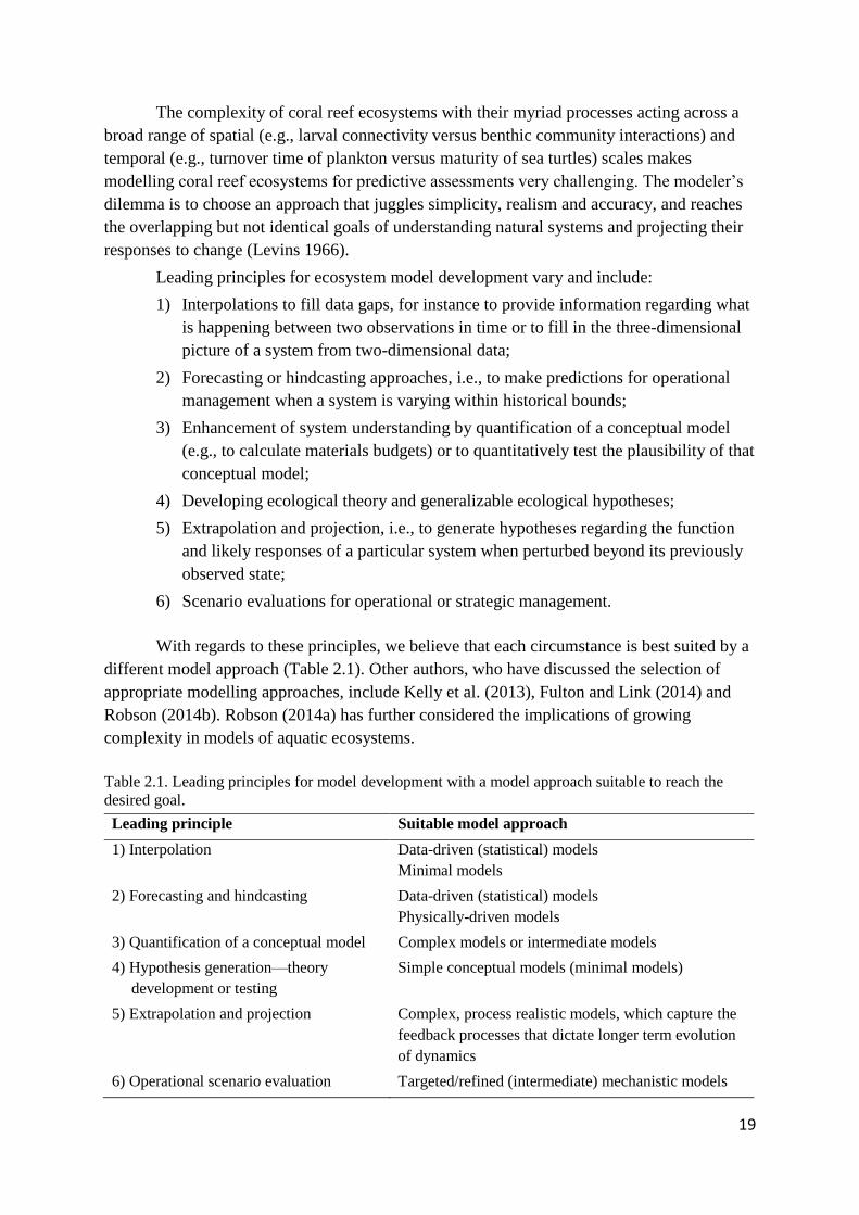
Leading principles for ecosystem model development vary and include:
1) Interpolations to fill data gaps, for instance to provide information regarding what
is happening between two observations in time or to fill in the three-dimensional
picture of a system from two-dimensional data;
2) Forecasting or hindcasting approaches, i.e., to make predictions for operational
management when a system is varying within historical bounds;
3) Enhancement of system understanding by quantification of a conceptual model
(e.g., to calculate materials budgets) or to quantitatively test the plausibility of that
conceptual model;
4) Developing ecological theory and generalizable ecological hypotheses;
5) Extrapolation and projection, i.e., to generate hypotheses regarding the function
and likely responses of a particular system when perturbed beyond its previously
observed state;
6) Scenario evaluations for operational or strategic management.
With regards to these principles, we believe that each circumstance is best suited by a
different model approach (Table 2.1). Other authors, who have discussed the selection of
appropriate modelling approaches, include Kelly et al. (2013), Fulton and Link (2014) and
Robson (2014b). Robson (2014a) has further considered the implications of growing
complexity in models of aquatic ecosystems.
Table 2.1. Leading principles for model development with a model approach suitable to reach the
desired goal.
Leading principle Suitable model approach
1) Interpolation Data-driven (statistical) models
Minimal models
2) Forecasting and hindcasting Data-driven (statistical) models
Physically-driven models
3) Quantification of a conceptual model Complex models or intermediate models
4) Hypothesis generation—theory
development or testing
Simple conceptual models (minimal models)
5) Extrapolation and projection Complex, process realistic models, which capture the
feedback processes that dictate longer term evolution
of dynamics
6) Operational scenario evaluation Targeted/refined (intermediate) mechanistic models

20
Models, suited for coral reef managers who need to define management strategies for
the entire coral reef ecosystem, need to consider interactions among system components and
management sectors as well as cumulative impacts of disturbances to the system (Rosenberg
and McLeod 2005, Kroeker et al. 2013, Ban et al. 2014). Ecosystem understanding should
include the human component in terms of their social and economic dependencies on these
marine resources (Liu 2001, Nyström et al. 2012, Plagányi et al. 2013). Management
scenarios that enhance the biological state might be unfavorable for the local economy,
especially on short time scales. Responses of slow-reacting systems, such as coral reefs,
could diminish community support for effective management. Still, they also give managers
an opportunity to act before a new, less favorable, condition has established itself (Hughes et
al. 2013). To date, few tools have been available that evaluate the socio-economic and
ecological tradeoffs of management scenarios of an ecosystem-based approach to coral reef
management. Coral reef ecosystem models that do include the human component are mostly
focused on fisheries management with socio-economic impacts presented as changes in
catches or landings (McClanahan 1995, Gribble 2003, Shafer 2007, Tsehaye and Nagelkerke
2008). Few models dynamically couple ecological dynamics to socio-economic drivers and
these models also focus on fisheries management (Kramer 2007) with Melbourne-Thomas et
al. (2011b) including a combination of fisheries, land-use and tourism.
The modelling approach most suitable to reach specific goals for ecosystem-based
management depends on the type of governance (e.g., existing laws and enforcement), time
and space scales under consideration, and data availability (e.g., data quantity, quality and
accessibility; Tallis et al. 2010), as well as the maturity of scientific understanding of the
system under consideration and the time and resources available for model refinement and
validation (Kelly et al. 2013). The concepts encompassed by Management Strategy
Evaluation (MSE) or Decision Support System (DSS) tools are a useful way of exploring
management issues that can be applied to many model types. MSE involves simulation
testing of alternative combinations of monitoring data, analytical procedures and decision
rules to give insight in the implications for both the resource and the stakeholders, and can be
used for evaluating the tradeoffs between socioeconomic and biological objectives (Smith et
al. 2007). In situations when neither data nor time is a limiting factor for model development
and site-specific management scenarios need to be simulated, ‘end-to-end’ or ‘whole-of-
system’ models can be developed for the MSE. In more data-poor or time-limited situations
or when less-specific scenarios with processes that are easily traced back are required,
‘minimum realistic’ models can be used as a basis of the MSE (Plagányi et al. 2013).
Alternatively simple, even qualitative, models can be used to shed light on ecological (or
other system) concepts, helping stakeholders to think about topics important in defining
effective management strategies (Tallis et al. 2010) or these simpler models can be used as
the logical basis of the MSE in their own right, as per Smith et al. (2004).
Drawing in all models of reef systems would be intractable, especially given the
number of conceptual models that exist in the mainstream and grey literature. Consequently,
we have put particular emphasis on their usefulness for evaluating the ecological implications
of model applications for MSE (as that is where our expertise largely lies) and we constrain
our review to the strengths and limitations of ‘dynamic’ coral reef ecosystem modelling

21
approaches in their application to management scenario analyses. We define a ‘dynamic’
model of a given system as a set of mathematical formulations of the underlying processes in
time and/or space with outputs for each time step over a specified period. With such a model,
the development of the system in time and space can be simulated by means of numerical
integration of the process formulations.
This review is not an exhaustive comparison of all dynamic coral reef ecosystem
models but we have selected studies that employ commonly used or exemplar approaches
that represent model types categorized as ‘minimal’, ‘intermediate’ and ‘complex’ models.
This classification was based on a scoring system that combined (1) their level of realism
(determined by the conceptualism of space, time and structure) and (2) the process details
incorporated into the model (Table 2.2). Additionally, we looked at the leading principle for
development of each model (Mooij et al. 2010). We contend that the leading principle of
minimal dynamic models is understanding the type and shape of the response curve of
ecosystems to disturbances. The leading principle of complex dynamic models is to predict
the response of ecosystems to disturbances under different management regimes given the
many feedbacks in the system. Intermediate dynamic models try to balance between these
two objectives. They do so by expanding parts of the system to the full detail while
deliberately keeping other components simple. In this way they can capture some key
feedbacks while maintaining the tractability of simple models, meaning they can make use of
analytical and formal fitting procedures (Plagányi et al. 2014). We highlight the differences
between the model approaches, discuss their main goals and outline the approach to take the
strength of the different modelling types to obtain clarity and predictive capabilities in a
model.
2.2 Categorization of three coral reef model types: Minimal, intermediate and complex
The rationale for any model is the desire to capture the essence, and to remove or reduce the
redundant aspects, of the system under study. What is essential and what is redundant and,
thereby, what level of reduction is required, to a large degree depends on the questions being
asked, the available information to base conceptualizations on and the way in which
abstractions are formulated. The result is a ‘model’ that is realistic to varying degrees. It is
not a clear cut recipe book approach as modelers need to define the tradeoffs between
temporal and spatial resolutions, taxonomy and model structure, as well as model detail, i.e.,
between comprehensiveness and complexity. Using 27 published studies that we felt were
representative of reef models in the literature, we classified the dynamic coral reef models
along an axis of model type (Tables 2.3 and 2.4) to get a greater understanding of how
differently sized models can be used in coral reef ecosystem management, particularly in the
context of MSE. We first classified models primarily on basis of their leading principle.
However, while categorizing models in terms of all of these facets separately is possible it is
difficult to think in such hyper dimensional spaces, so to facilitate comparisons we then
mapped models to a simple continuum of simple to complex via a scoring system (Table 2.2;
for scoring results see Weijerman et al. 2015).

22
Table 2.2. Complexity scoring of various criteria to classify models or model applications.
Criteria/Score 1 2 3 4 Comments
Conceptualization
of structure
# plankton grps 0 1-2 3 > 3 groups can be individual
species or aggregated
species groups
# benthic grps 1 2 3-4 > 4
# invertebrate grps 0 1-2 3-4 > 4
# vertebrate grps 0 1-2 3-5 > 5
Conceptualization
of space
non-
spatial lumped
grid or
cell based
lumped has a single output
of entire modelled area; grid
or cell based represents
uniform or non-uniform grid
or vectors
Process Details
trophic interactions
inter/intra species
competition
age structure
biogeochemistry
hydrodynamics
2.2.1 Minimal models
With few mathematical equations, minimal dynamic models are often used as a
toolkit for the development of ecological theory. Minimal models have proven to be a helpful
tool in gaining fundamental insight into the complex dynamics of a specific system (i.e.,
chaos, cycles, regime shifts, etc.). In coral reefs, for example, they have played an important
role in conceptualizing and understanding observed regime shifts (Hughes 1994, Mumby et
al. 2013b). Generally, people do not intuitively consider nonlinear responses, i.e., we often
assume that a small change in environmental conditions will lead to a small (or at least
consistently proportional) change in the ecosystem. Minimal models have been used to show
what kind of surprises could arise when nonlinear interactions between system variables (e.g.,
feedback mechanisms) are taken into consideration (#1 in Table 2.3). Using minimal models
to simulate coral reef dynamics, fundamental insight into thresholds (#1), primary drivers of
system dynamics (#2, 3), the type of system response to changing conditions and the effect of
hysteresis can thus be gained (#4). Recently, the interaction between ocean acidification and
warming and coral growth/cover has been examined with minimal models (#5). Some
minimal models also incorporate local environmental changes (e.g., nutrient input, hurricanes
and fishing) to study coral cover response and are able to forewarn whether current levels are
precautionary or whether new challenges are coming (#6). Early minimal models examined
the main drivers of reef accretion and erosion processes (#7–9). Gaining insight in these
important aspects of a system’s response to current or future perturbations can help managers

23
to understand observed surprising dynamics, focus on the most relevant (sensitive) variables
and to conservatively move away from tipping-point thresholds by increasing reef resilience.
While, to the authors’ knowledge, there is currently no published MSE using a simple reef
model as a basis, the response curves derived from such models could be used as the basis of
a qualitative MSE of the form undertaken in a temperate system by Smith et al. (2004).
One advantage of minimal models is their ability to thoroughly explore the behavior
of the model in a multidimensional parameter space by using analytical or numerical
methods. This way, the relative importance of specific processes or interactions can easily be
traced back. However, minimal models ignore other potentially important phenomena that
affect a system’s behavior (Scheffer and Beets 1994). Moreover, they often assume spatially
homogenous conditions and constant environments. Reefs have patchy distributions of corals
and fish, often determined by environmental factors (Franklin et al. 2013), so including
spatial dimensions explicitly in the model can greatly improve the realism of reef dynamics.
However, explicit spatial representation is not automatically required, so long as careful
thought is given to how to implicitly represent the spatial influences. Because minimal
models lack the link between all trophic groups and the response of multiple stressors, they
can be less suitable in a multispecies or multidisciplinary decision-making context. Minimal
models have paved the way for the theory on generic early warning signals of tipping points
(Scheffer et al. 2009). While minimal models themselves are likely to be too simplistic to
precisely predict future behavior in systems that are not already well understood, early
warning signals may be an important additional tool for ecosystem managers.
Based on the leading principle defined for minimal models, nine models could be
classified as minimal models developed to enhance understanding of the type and shape of
the response curve of ecosystems to disturbances (#1–9). According to our scoring system,
the overall complexity score, based on the mean score of model structure, representation of
space and process details, varied between 2.3 and 4.4 with a mean score of 3.3 (Weijerman et
al. 2015) The box model (#7, 8) had an overall score of 4.4 and could also be placed in the
intermediate category, whose overall score was between 3.0 and 5.0 with a mean of 4.1.
2.2.2 Intermediate models
Intermediate models are more focused than typical whole-of-system models; they try to
marry the strengths of simple models (in terms of tractability) with a broader system
perspective to selectively link the key drivers of the system. These models simulate species-
specific behavior and age or size structure with a set of mathematical formulas, capturing the
population dynamics of key functional groups and potentially their spatial heterogeneity if
spatially explicit (Plagányi 2007). These kinds of models typically include at least one key
ecological process (e.g., a link to lower trophic levels, interspecific interactions or habitat
use) and potentially some representation of how the modelled components are affected by
physical and anthropogenic drivers (Plagányi et al. 2014).
The leading principal for this type of model was defined as trying to find a balance
between system understanding and predictive capabilities by expanding parts of the system to
the full detail while deliberately keeping other components simple. For example, by including
more details on process dynamics but limiting the functional groups (#15, 18), a greater

24
understanding was reached of the population dynamics and perturbations (fishery [#15] and
environmental factors [#18]) of that specific group. This more realistic and heterogeneous
system representation provides information about a system that is not available from a
minimal model. In pointing to a representative example of an intermediate complexity reef
model there are a number of potential candidates. Two clear classes of questions have been
tackled with these kinds of models. The first is around using multispecies or trophic models
to explore the coral reef ecosystem impacts of fishing (Table 2.3, #10–16, 19) and the second
uses models, often individual or agent-based models (Grimm et al. 2006), to consider how
competing habitat defining groups respond to changing conditions (#17, 18, 20, 21).
The Ecopath and Ecosim (EwE) modelling platforms (Polovina 1984, Walters et al.
1997, Pauly et al. 2000) is one of the most commonly used model type for exploring trophic
connections and responses to fishing pressure. Although the suite of EwE models can be
considered complex based on our criteria (Table 2.2), the application of EwE models in the
selected studies has been mostly to look at just one disturbance (fisheries) through expansion
of that part of the model components while leaving the rest simple (e.g., few functional
groups, no inclusion of Ecospace or life cycle (age-structured) processes) and, hence, the
leading principle fits with our classification of ‘intermediate’. Similarly while some agent-
based models can be considered complex in terms of the elaboration of particular ecological
mechanisms, in the context of their use in coral reef ecosystems they have often been used as
intermediate complexity models. When EwE is used to explore reef dynamics it can give
insight into a system’s ‘state’ based on changes in energy flows as a response to perturbation
(#10, 12 and 13) and multiple positive or negative feedback loops can be included with this
model approach (#17, 21 and 22). The classification of EwE models also illustrates that
modelling platforms often do not simply slot into one category but can be simple,
intermediate or complex depending on the details of a particular application. For example,
one application of EwE, for examining fishery scenarios for Indonesian reef systems,
included 98 tropic groups and three of the five selected process dynamics (#14) and was used
for evaluating management scenarios. Thus it was categorized as complex (Table 2.3) as its
overall complexity score of 6.0 sits within the span of scores (5.3 to 6.8, mean 5.9;
Weijerman et al. 2015) of complex models.
A disadvantage of intermediate models is that the software code often consists of
linked models, which complicates the interpretation of results (Lorek and Sonnenschein
1999). Additionally, because of the need for more parameters, variables and model
formulations, each with their own uncertainties, model output becomes less certain or robust
(Pascual et al. 1997) and validation and sensitivity analyses are more cumbersome (Rykiel Jr
1996). Nevertheless these models are still simple enough that good use can be made of formal
statistical estimation procedures originally developed for simpler models (Plagányi et al.
2014).
Management applications of intermediate models include the ability to inform
managers where a system is on a gradient from ‘pristine’ to degraded/disturbed so that
effective action can be identified and implemented (McClanahan 1995, Kramer 2007).
Additionally, especially with respect to the suit of EwE models that have been used for
fishery management strategy evaluation, this model approach gives valuable insight into

25
ecosystem impacts of alternative fishery scenarios. However, spatial factors, nutrient
dynamics, benthic processes and extrinsic forcing functions are not always included in
intermediate models but can be important for projecting the effects of some perturbations on
ecosystems (Robinson and Frid 2003).
2.2.3 Complex models
What we categorized as complex models are often called end-to-end models or whole-of-
system models. These models typically include a food web spanning a set of trophic groups:
detritus, primary producers, zooplankton ranging from small (µm) to large (m) animals,
forage fish, invertebrates and apex predators, including humans. They also often explicitly
simulate biogeochemical dynamics. For coral reefs that are surrounded by oligotrophic water,
nutrients play a key role in ecosystem dynamics. Including biogeochemical processes in a
coral reef ecosystem model is, therefore, essential to simulate these processes, especially
since land-based sources of pollution have played an important role in the demise of many
reef systems in the Caribbean (Lapointe 1997) and on the Great Barrier Reef (De’ath et al.
2012). In comparison with the other two model types, additional key ecosystem processes
(e.g., trophodynamics and feedback loops) are represented to more comprehensively simulate
a system’s behavior. These complex models aim to provide quantitative projections of system
changes in response to a set of changing abiotic and biotic conditions taking into account key
components and their spatial heterogeneity (in some cases from microbes to whales and
humans, and from sediment bioturbation to physical oceanography). Simplicity is sacrificed
as these models are simultaneously complex in many dimensions (process details, number of
functional groups, nutrients, spatial and temporal dimensions, see Table 2.3 #23–27). That is
not to say every component or aspect is resolved in fine detail. Such an approach does not
lead to useful outcomes; tradeoffs between the dimensions are nearly always required so as
the scope or the number of scales extends sacrifices are likely required in other facets (such
as using growth terms rather than very finely resolved physiological representations of each
ecological process for each modelled group).
Representing a system in this way can be advantageous for capturing trophic cascades
and synergistic effects of perturbations, as the model implementation explicit includes (1) key
functional groups at each trophic level (Mitra and Davis 2010) and (2) model complexity
varies with details where needed in terms of number of functional groups and compatibility
between lower and upper trophic level formulations (Fulton et al. 2003a). These models can
represent many more of the myriad nonlinear, two-way interactions than simple or
intermediate models represent. Humans are an integral component of most complex models,
both as users of ecosystem services and as drivers influencing ecosystem processes (Levin et
al. 2009).
The major drawback of these model types is similar to that of intermediate models:
the addition of complexity does not guarantee an improvement in the simulated output as
uncertainty and error associated with the added components will be introduced to the model
and can potentially degrade its performance. Uncertainty arises both from assumptions made
in the model structure and from uncertainty around the values of parameters, amongst other
sources (Draper 1995, Renard et al. 2010).
26
The difficulties of properly understanding the implementation of ecological and socio-
economic processes in a complex model hamper straightforward validation and could lead to
less reliable projections. To improve the performance of complex ecosystem models, studies
have looked into the effects of trophic aggregations (Gardner et al. 1982, Fulton 2001), model
structure (Ruiz Sebastián and McClanahan 2013), physiological detail (Fulton et al. 2004a,
Allen and Polimene 2011), spatial representation (Fulton et al. 2004c), predator-prey
relationships including age-structure (Botsford et al. 2011) and inter-predator competition
(Walters and Christensen 2007). Best practice guidelines for developing complex models
have been formulated (Fulton et al. 2004b, Flynn 2005, FAO 2007, Travers et al. 2007).
Some of these recommendations are (1) the inclusion of functional groups at low trophic
levels and species of higher trophic levels with an appropriate spatial dimension to represent
organism dynamics more accurately; (2) inclusion of abiotic processes to simulate important
drivers in structuring ecosystem communities; (3) the integration of physical and biological
processes at different scales (relevant to the scales of key processes) to more realistically
simulate those dynamics; (4) evaluating the model in terms of its ability to reproduce
expected patterns from ecological theory and in terms of the degree to which it accords with
current biophysical understanding of the system; and (5) two-way interactions between
ecosystem components to allow dynamic feedback and nonlinear dynamics to emerge.
Most complex coral reef models are developed to assess the cumulative effects of
climate change, fishing (#25, 26) and water quality (#27) on ecosystem dynamics and the
resilience of coral reefs under simulated management scenarios (#23, 24). Through the
inclusion of the breadth of the food web and many alternative interaction pathways, non-
intuitive (and, therefore, unanticipated) outcomes in community structure can present
themselves. It should be noted that unexpected, chaotic and non-linear system dynamics can
be exhibited by simple models, again simply including more components does not guarantee
revelations outside the purview of other approaches. Not only the number of groups
represented, but also the number and types of interactions between them is important (Baird
2010, Takimoto et al. 2012). The main consideration is the inclusion of mechanisms of
achieving alternative outcomes—multiple reaction pathways that can reach alternative stable
states. The same logic is behind why the inclusion of humans and their activities in model
simulations facilitates further evaluation of tradeoffs between ecosystem services and
management goals. This information can then support the identification of policies and
methods that have the potential to meet a priori stated objectives (Levin et al. 2009).
Although there is a continuous scale from minimal to complex model approaches, we
differentiated between three categories (minimal, intermediate or complex) based on the
leading principal for model development and on their overall complexity score related to the
model conceptualism and process detail (Table 2.3). The mean complexity score reflects this
continuous scale as model approaches overlap between the three categories. As we go from
simple to complex models, a tendency in the leading principle is visible—from understanding
towards prediction and projection. The desired balance between these two objectives in a
given study could therefore give some indication of the appropriate level of model
complexity.

27
Table 2.3. Selected dynamic coral reef ecosystem models and model applications categorized as minimal, intermediate and complex based on their system
conceptualization and process detail (Table 2.2). For overall complexity score calculations, see (Weijerman et al. 2015).
# Model Source Reef area Leading principal Suitable for MSE
Category based on
leading principle
Overall
Score
1 Caribbean reef model Mumby et al. 2007a Caribbean fore-reef System understanding of coral-
algae dynamics
Insight in benthic
dynamics
Minimal 2.3
2 Bayesian Belief Network
model
Renken and Mumby
2009
Caribbean fore reef System understanding of
macroalgal dynamics
Insight in benthic
dynamics
Minimal 3.3
3 HOME model Wolanski et al. 2004 Great Barrier Reef
& Guam
System understanding of coral-
algal dynamics
Insight in benthic
dynamics
Minimal 4.3
4 Community model Żychaluk et al. 2012 Kenya, Caribbean,
Great Barrier Reef
System understanding of
occurrence of alternative
ecosystem states
Insight in benthic
dynamics
Minimal 2.8
5 Community model Anthony et al. 2011 Caribbean System understanding in benthic
dynamics under climate change
Insight in benthic
dynamics
Minimal 3.4
6 Deterministic model Blackwood et al.
2011
Caribbean System understanding of coral-
algal dynamics including reef
complexity
Insight in reef resilience
in relation to fishery
Minimal 2.9
7 Box model Eakin 1996 25,308 m2 Uva
Island, Panama
System understanding of reef
accretion/ erosion processes
Insight in reef
complexity
Minimal 4.4
8 Box model Eakin 2001 25,308 m2 Uva
Island, Panama
System understanding of reef
accretion/ erosion processes
Insight in reef
complexity
Minimal 4.4
9 ReefHab Kleypas 1997 Generic reef
(parameterized for
Mesobarrier Reef
Caribbean)
System understanding of reef
accretion/erosion processes
Insight in environmental
factors limiting reef
habitat
Minimal 2.6
10 Energy-based model McClanahan 1995 Generic local reef
(parameter-ized for
Kenyan reef)
System understanding of effect of
fishing on ecosystem structure
and fishery yield
Insight in tradeoffs of
alternative fishery
scenarios
Minimal/
Intermediate
5.0
11 Ecopath with Ecosim Tsehaye and
Nagelkerke 2008
6000 km2 Red Sea
Fisheries effects on ecosystem -
change in fishery scenarios
Insight in ecosystem
impacts of alternative
Intermediate 4.1

28
# Model Source Reef area Leading principal Suitable for MSE
Category based on
leading principle
Overall
Score
fishery scenarios
12 Ecopath with Ecosim Weijerman et al.
2013
Hawaii Identify indicators for fishery for
management - change in fishing
intensity
Insight in ecosystem
impacts of increased
fishing
Intermediate 4.5
13 Ecopath with Ecosim Arias-González et
al. 2004
Mexico Fisheries effects on ecosystem -
change in fishery scenarios
Insight in ecosystem
impacts of alternative
fishery scenarios
Intermediate 3.9
14 Ecopath with Ecosim Ainsworth et al.
2008
Indonesia Fisheries effects on ecosystem -
change in fishery scenarios
Insight in ecosystem
impacts of alternative
fishery scenarios)
Complex 6.0
15 Effects of Line Fishing
Simulator (ELFSim)
Little et al. 2007 Great Barrier Reef Understanding of population
dynamics of single species under
alternative fishery scenarios
Evaluate tradeoffs on
population dynamics of
1 species under
alternative fishery
scenarios
Intermediate 3.0
16 Individual-based model Edwards et al. 2011 Caribbean mid-
depth fore-reef
System understanding of
disturbance impacts under
alternative fishery scenarios
Insight in resilience of
benthic community from
disturbances under
different fishery
scenarios
Intermediate 4.6
17 Individual-based model Wakeford et al.
2007
32 m2 Lizard
Island, Great
Barrier Reef
System understanding (coral
community dynamics after
perturbations) and projected
trajectory under future drivers
Insight in reef resilience
in relation to
disturbances
Intermediate 3.8
18 Spatially-explicit Reef
Algae Dynamic
(SPREAD) (individual-
based)
Yñiguez et al. 2008 Florida, 3-D cells
of 1x1 cm
System understanding
(macroalgal growth and
morphology)
Insight in environmental
factors influencing
macroalgal dynamics
Intermediate 4.4

29
# Model Source Reef area Leading principal Suitable for MSE
Category based on
leading principle
Overall
Score
19 Lotka-Volterra model ~
adaptive behavior model
Kramer 2007 Generic Caribbean
reef
Understanding in coupling
between biological and fishery
dynamics
Effects of fishery on
ecosystem state and vice
versa
Intermediate 5.0
20 Cellular automaton
model
Langmead and
Sheppard 2004
Caribbean System understanding (coral
community restructuring
processes after disturbance)
Insight in reef resilience
in relation to
disturbances
Intermediate 4.1
21 Biogeochemical ~
hydrodynamic model
Faure et al. 2010 2066 km2 lagoon,
New Caledonia
System understanding (ecosystem
variability under environmental
disturbances)
Insight in
biogeochemical response
under different scenarios
Intermediate 3.4
22 Ordinary Differential
Equation-based model
Riegl and Purkis
2009
Generic
(parameterized for
Arabian/Persian
Gulf)
System understanding of coral
community structure and recovery
after multiple bleaching events)
Insight in coral
community structure
after repeated
disturbances
Intermediate 3.8
23 Coral Reef Scenario
Evaluation Tool
(CORSET)
Melbourne-Thomas
et al. 2011a
1342 km2 (5-20 m
depth) Generic reef
ecosystem
Decision support tool with
simulations based on 'what if'
scenarios
Projecting reef futures
under different scenarios
Complex 6.8
24 Ordinary Differential
Equation-based model
Fung 2009 Generic local reef System understanding (key
ecological processes related to
degradation) and scenario testing
Projecting reef futures
under different scenarios
Complex 5.3
25 Integrated agent-based
model
Gao and Hailu 2011 ~6000 km2,
Ningaloo Marine
Park, Australia
Decision support tool with
simulations based on 'what if'
scenarios
Site closure strategy
analyses
Complex 5.4
26 Coral-Algae-Fish-
Fisheries Ecosystem
Energetics (CAFFEE)
Ruiz Sebastián and
McClanahan 2013
Kenya Model structure understanding,
calibration methods
Insight in reef resilience
related to fishery and
environmental drivers
Complex 6.1
27 eReefs Schiller et al., 2013;
Wild-Allen et al.,
2013; Mongin and
Baird, 2014
300000 km2, Great
Barrier Reef,
Australia
Support tool for rapid response
and slow response management
and system understanding
Projecting reef futures
under different land
management scenarios
Complex 6.8

30
2.3 Multiple model strategies in relation to coral reef management
2.3.1 Combining models of different complexity
Modelling is an art that balances simplicity, realism and accuracy of various dimensions
(Levins 1966): time, space, trophic components, process details, human activities, boundary
conditions and forcings. Considering coral reef management, all model formats have their
pros and cons. However, insights gained by one model can be useful for the application of
another (Mooij et al. 2009). Moreover, multiple model types can be combined. Their
outcomes go beyond possible outcomes from a single model alone. Approaches combining
models include:
The ‘three-stage rocket approach’, in which first mini-models and then
intermediate models can be used to identify the relevant variables or processes to
steer on. The resulting intermediate model can then provide a basis for the
complex model, with the aim of reaching a projection that is based on
understanding. A variant of this approach is to couple models of different forms
and origin to piece together a more complete representation of the system. Such
approaches are becoming increasingly popular in the research community, but
care must be taken to understand how to propagate error and deal with scale
differences between the model types.
The ‘build then refine approach’, in which a complex model is used to identify
key drivers of system responses, which can then be used to develop simpler, faster
models or statistical emulators, whose behavior can be more thoroughly
characterized, providing more accurate predictions for a more limited range of
scenarios (Robson 2014b).
But, as discussed in the following paragraphs, there are more ways in which we can
benefit from combining modelling approaches, including the ‘peeling off complexity
approach’, which is the opposite in form to the ‘three-stage rocket approach’.
2.3.2 From understanding to projecting
Minimal models are important for the development of concepts and theory; they examine
how certain phenomena can be reproduced and so reveal general explanations. They are also
helpful in identifying and getting insight into processes that cause nonlinear system behavior.
As such, minimal models can provide a conceptual framework wherein management
scenarios can be explored. They can help managers to address the right questions, i.e., which
process details and variables to focus on. Intermediate models include enough detail to couple
different concepts and test these concepts relative to each other and relative to other factors,
such as external forcings (e.g., nutrient input, hurricane damage) and simplistic management
scenarios. Improved understanding is still the main aim of this model type, although the
increased complexity requires more effort to trace underlying mechanisms. When the
understanding of key ecological or socioeconomic processes is sufficiently enhanced one can
continue with making projections. However, some of the questions raised by ecosystem

31
managers are beyond intermediate models, as they miss the necessary details in the model
conceptualism or the full suite of key ecosystem processes.
Model complexity can arise either by increasing the detail at which particular
compartments or processes are represented or by broadening the scope of the model, for
instance, moving from a model of coral biology to a model of coral reef ecosystems to a
model that also includes the human behaviors that affect those ecosystems. Many very
complex biogeochemical models are narrowly focused, while broadly focused, integrated
economic-ecological-biophysical models often represent their individual components with
much less detail.
Well-formulated and comprehensive complex models are suitable for evaluating
social, economic and ecological tradeoffs of alternative management scenarios but typically
lack the straightforward validation needed to fully understand the model’s projection
capabilities. Very complex models may be too cumbersome to embed in end-user focused
decision-support tools and may be too computationally intensive to allow large numbers of
scenarios or optimization runs to be conducted. They may also lack transparency, which
(when these models are used without also employing simpler models) can make it difficult
for policy makers to develop confidence in the models and insight into the tradeoffs and
processes represented in the models.
2.3.3 Including socio-economics
Intermediate and complex models are difficult to parameterize, analyze and validate and have
a long development time. Because they often contain input from many experts, the model
code may be less transparent and harder to maintain and debug, and the performance of these
models is rarely thoroughly assessed. However, if these challenges can be overcome, they can
include the whole ecosystem and socioeconomic components and so can be instrumental for
management options and strategy evaluations (Plagányi 2007). For coral reef ecosystems
such models are rare. From the 27 reviewed model studies, only three model approaches
explicitly included human socioeconomic drivers (Table 2.3, EwE model [#14], coupled
biological and Bayesian human behavior model [#18] and an integrated agent-based model
[#25]), although in some models, fishing activity is implicit in the model parameterization
(e.g., EwE models [#11–14]). The significance of a change in ecosystem state to fisherman or
the feedback between fishing pressure and ecosystem state (Cinner et al. 2009, Cinner et al.
2011) are important components for successful management (Hughes et al. 2010, Plagányi et
al. 2013).
2.3.4 ‘Peeling off’ approach
As said above, a major criticism of complex models is the difficulty in understanding the
underlying mechanisms of their outcomes. To improve our understanding of the way in
which these models generate their results we need to peel off the many layers of complex
models to effectively reduce their output to explore the key feedback mechanisms and their
response to changes in conditions (van Minnen et al. 1995, Van Nes and Scheffer 2005b).
Tools to do this include sensitivity analysis, network analysis of model output and
construction of materials budgets to trace dominants pathways of carbon, energy or nutrients

32
through the system. This approach helps to base complex models upon a proper
understanding of the feedback mechanisms explored in minimal models and only those
dynamic mechanism and responses that are key to the system’s behavior should be
incorporated (Fulton et al. 2005), keeping in mind that synergistic effects may occur. This
resulting set of mechanisms and responses should then be augmented by incorporating spatial
and environmental parameters that are thought to cause shifts in system states and for which
these relationships between state variables were explored (van Nes and Scheffer 2005a). In
this approach the results of complex model can be better validated using existing ecological
theory and empirical data.
2.3.5 Stability versus complexity
Another recurring criticism of complex models is that community models (e.g., based on
Lotka–Volterra equations) become increasingly unstable as complexity increases (May
1972). However, field and experimental observations have shown that ecosystem complexity
enhances resilience and stability (Folke et al. 2004, Hughes et al. 2005, Friedrichs et al. 2007,
Burgess et al. 2013, Pasari et al. 2013). Previous work has shown the critical role of space as
a resource in marine systems, combating the complexity-stability conflict (Fulton et al.
2004c). Moreover, findings from food-web theory show that to improve a model’s stability,
the modelled food web should consist of multiple trophic levels and capture other food-web
features, for example, weak links and mechanisms that weaken the interactions, such as,
asymmetric feeding and non-feeding interactions (Fulton et al. 2003a, Rooney et al. 2006,
Neutel et al. 2007, Travers et al. 2010). When models include sufficient interactions,
simulated community stability increases rather than decreases with model complexity (Baird
2010).
Most dynamic ecosystem models include non-linear functional response curves that
greatly contribute to system stability, for example, when predators are capped by a carrying
capacity they can no longer drive prey to extinction. Also refugia, migration or dispersal
terms and adaptive behavior or plasticity can be built into models to prevent species from
dying out completely. However, particularly in more complex models, justifying the use of
all these stabilizing mechanisms is difficult, as it is often challenging to obtain realistic
parameter values and identify the actual shape of each response curve. The uncertainty of
parameters and the complexity of the model makes it difficult to foresee the consequences of
model behavior other than bringing stability, i.e., even if the model fit is good, it may be
based on the wrong assumptions. Sensitivity analysis and peeling off complexity at the level
of these stabilizing mechanisms could provide the required insights.
2.3.6 Ensemble modelling
A way to deal with limits on predictability is to run a complex model with different initial
conditions and model formulations and explore the outcomes to assess the likelihood of
certain events rather than give a single deterministic or tactical projection (Hannah et al.
2010). This approach is called ensemble modelling (another form of ensemble modelling is to
compare the results of the application of different model frameworks to the same scenario,
see below). Outcomes can then be compared with multiple minimal models for confirmation

33
of results (Fulton et al. 2003a), with long term field data (Ruiz Sebastián and McClanahan
2013) or expert judgment (Mauser et al. 2013). Often, the most interesting and useful results
are obtained when the model does not agree with expert judgment, as this indicates either (i)
a fault in the conceptualization of the system as represented by the model, which indicates
that further thought or research is needed, or (ii) the potential existence of an unforeseen
system behavior that could have implications for management.
Another form of ensemble modelling is when different models are applied to a single
system. The resulting bandwidth of outcomes can give insight in the ‘structural uncertainty’
of the inevitable artifacts in the model formulations (Trolle et al. 2014). This type of
uncertainty can only be studied by concurrently applying multiple models and as this
approach is rarely taken this type of uncertainty is often ignored. Despite the fact that
handling and quantification of uncertainty in model output arising from uncertainty in the
numerical inputs to the model (e.g., parameters, initial conditions, forcing functions,
boundary conditions) is the typical focus of the published literature (e.g., Hoeke et al. 2011,
Pandolfi et al. 2011, Yara et al. 2014 for uncertainties related to climate change and coral reef
trajectories), structural uncertainty is often larger and has more significant implications for
decision-makers.
2.4 Concluding remarks
This review of model types illustrates that much can be gained from investing time in
appreciating the identity and potential of each of the three model types in its own right and in
concert. Each of the discussed model types can be helpful, but each also has limitations, when
used in a management-oriented context. Minimal coral reef models are crucial in our
understanding of ecosystem feedback loops and their response curves. Understanding the
drivers of change in a system’s state will improve effective management responses—to
reverse, prevent or mitigate this change. Intermediate models can assist managers with
projections of ecosystem responses and indirect outcomes through the inclusion of a broad
(but potentially still incomplete) set of key system components. Intermediate coral reef
models can be used to answer many questions as they not only include key biological
components, but also various environmental or anthropogenic drivers. For some questions
(e.g., when there are multiple interacting drivers) more complex models are the most
informative decision-support tools, as they include the major dimensions (i.e., spatial,
temporal, taxonomic, nutrient, human activities) and, therefore, incorporate the often
cumulative effects of various dynamic mechanisms and responses that are beyond what can
be represented in minimal or intermediate models that sacrifice on these dimensions in return
for tractability in understanding the model outcomes. For example, system-level models are
useful for evaluating the economic and ecologic tradeoffs of various management scenarios,
as these more complex models contain the extra detail that is required to capture the
feedbacks of interest. However, complex models are not suitable in all situations; in many
cases managers value the speed and transparency of simple models.

34
Nudibranch on crustose coralline algae. Photo NOAA

35
Chapter 3
Coral reef ecosystems and performance
indicators
Weijerman, M, EA Fulton, FA Parrish. 2013. Comparison of coral reef ecosystems along a
fishing pressure gradient. PLoS ONE 8:e63797.

36
Three trophic mass-balance models representing coral reef ecosystems along
a fisheries gradient were compared to evaluate ecosystem effects of fishing.
The majority of the biomass estimates came directly from a large-scale visual
survey program; therefore, data were collected in the same way for all three
models, enhancing comparability. Model outputs—such as net system
production, size structure of the community, total throughput, production,
consumption, production-to-respiration ratio, and Finn’s cycling index and
mean path length—indicate that the systems around the unpopulated French
Frigate Shoals and along the relatively lightly populated Kona Coast of
Hawai`i Island are mature, stable systems with a high efficiency in recycling
of biomass. In contrast, model results show that the reef system around the
most populated island in the State of Hawai`i, O`ahu, is in a transitional state
with reduced ecosystem resilience and appears to be shifting to an algal-
dominated system. Evaluation of the candidate indicators for fishing pressure
showed that indicators at the community level (e.g., total biomass, community
size structure, trophic level of the community) were most robust (i.e., showed
the clearest trend) and that multiple indicators are necessary to identify
fishing perturbations. These indicators could be used as performance
indicators when compared to a baseline for management purposes. This study
shows that ecosystem models can be valuable tools in identification of the
system state in terms of complexity, stability and resilience and, therefore, can
complement biological metrics currently used by monitoring programs as
indicators for coral reef status. Moreover, ecosystem models can improve our
understanding of a system’s internal structure that can be used to support
management in identification of approaches to reverse unfavorable states.

37
3.1 Introduction
Resource managers are confronted with a range of challenges in their mission to sustain and
restore coral reef services that humans desire. Reductions in fishery harvests, whether a result
of the degradation of fish habitat, following declines of target fish population or increased
regulation, will have substantial cultural, economic, and social implications for resource
users. Effective management requires an understanding of coral reefs as ecosystems and of
the complex and potential synergistic effects of different drivers (McLeod et al. 2005, Levin
et al. 2009). Globally, about three-quarters of all coral reefs are threatened by increased stress
from pollution, extensive fishing and climate change (Burke et al. 2011). About half of the
coral species that are very susceptible to bleaching are also heavily vulnerable to disease and
predation, and recovery can be slow or absent (Carpenter et al. 2008). At the Great Barrier
Reef, coral cover has halved in the last three decades (De'ath et al. 2009). Ecological
processes will interact with effects of global environmental change. For instance, herbivores
(e.g., herbivorous fishes and sea urchins) can control the growth of algae and, therefore,
facilitate coralline algal and coral settlement and growth, and they have been identified as a
keystone group for their important role in structuring coral communities and improving reef
resilience, i.e., the ability of a reef to absorb shock, resist phase shifts, and regenerate after
natural and human-induced disturbances (Smith et al. 2001, Graham et al. 2006, McClanahan
1995, Nyström et al. 2000, Green et al. 2009). Reductions in herbivorous fish biomass also
may affect the microbial diversity with a shift to more pathogenic microbes and reduced
microbial species richness, ultimately affecting the condition of the reef (Bruce et al. 2012).
Areas protected from fishing or with less fishing pressure generally have higher live coral
cover than do unprotected areas, and fish communities have more large-bodied fishes (Selig
and Bruno 2010, Wilson et al. 2010). It is our opinion that management should focus on
assessment and improvement of reef resilience to maximize the capacity of corals to respond
to the imminent threats of global climate change (Hoegh-Guldberg and Bruno 2010, Graham
et al. 2011b).
Resource managers and users can benefit from an evaluation of the system’s present
status in terms of complexity, stability, and resilience—features that support biodiversity
(Odum 1971) and ecosystem ‘health’ (health used in terms of high diversity, energy
recycling, resilience) (Jørgensen et al. 2005). Fishing, habitat degradation, land-based sources
of pollution and global environmental changes all affect the health of coral reef ecosystems.
Coral reef models have been constructed to investigate ecosystem effects of fishing and
alternative fishery management scenarios (Walters et al. 1997, Arias-González et al. 2004,
Mumby 2006) habitat degradation (Gribble 2003, Ainsworth et al. 2008b), climate change
(Hoeke et al. 2011, Pandolfi et al. 2011) and land-based pollution (Wolanski et al. 2003a,
Mumby 2006). Despite the increase in number of modelling studies in coral reef areas, there
is still little information on the most appropriate indicators for changes in these systems (Link
2005). Outcomes from ecosystem-based models can identify quantifiable metrics that reflect
features of ecosystem’s structure and function, indicative for a system’s health under its level
and type of perturbations (Jørgensen et al. 2005, Link 2005). Establishing these indicators is
among the first steps scientists can take to support the implementation of ecosystem-based
management (Levin et al. 2009, Shin et al. 2010a). Once these indicators are identified, the

38
next step is to link them to criteria for management decisions; for example, indicator values
X, Y, and Z that fall below a priori established threshold values will trigger a specified
management action (Hall and Mainprize 2004). However, quantitative approaches for
selection of ecosystem-level indicators are only beginning to emerge and, so far, mostly for
pelagic systems (Fulton et al. 2005, Link 2005, Samhouri et al. 2009). These indicators might
not be suitable for coral reef ecosystems because reef systems differ in structure and energy
flow (e.g., more complex food webs, including the microbial food web, for effective
recycling of the limited nutrients in reef systems) and in fisheries (e.g., more diversified on
reefs).
Empirical studies on coral reef structure and function have generally used spatial
patterns or temporal trends in benthic cover and fish biomass and assemblages as indicators
for perturbations to reefs from terrestrial runoff (Stimson and Larned 2000, Fabricius 2005,
Storlazzi et al. 2009a), climate change (Eakin 2001, Anthony et al. 2008, McClanahan et al.
2011b) and fisheries (Friedlander and DeMartini 2002, Williams et al. 2008, DeMartini et al.
2010, Williams et al. 2011). These parameters are usually used as performance indicators for
reef health in monitoring programs. However, they target only direct effects of fishing and do
so mostly on small scales (e.g., fish biomass and size structure inside and outside marien
protected areas), and no indicators exist for indirect ecosystem effects. Such indicators are
crucial to an assessment of the overall ecosystem effects of target species removal and to
allow holistic fisheries management (Metcalf et al. 2011). Trophic mass-balanced models
represent an analytical approach that could help evaluate ecosystem effects of fishing
perturbations and identify optimal management scenarios (Walters et al. 1997, Arreguin-
Sanchez et al. 2004, Fulton et al. 2005, Diaz-Uribe et al. 2007, Smith et al. 2007, Xu et al.
2011).
This study focuses on the quantitative description of the characteristics of ecosystem
attributes of three coral reef systems along a fishing pressure gradient in Hawai`i, located in
the middle of the Pacific Ocean (Fig. 3.1). We attempt to identify the most reliable indicators
of ecosystem structure and function of coral reefs to support ecosystem-based fishery
management. This comparative approach along an exploitation gradient is used to identify a
range of indicators against which each system is assessed in relative terms. The model used is
validated with empirical assessments from field data, and the suitability of performance
indicators presently used for coral reef management in Hawai`i is discussed.
3.2 Methods
3.2.1 Study sites
We selected three systems along a gradient of fishing pressure on the basis of human
population and commercial catch statistics
(www.pifsc.noaa.gov/wpacfin/hi/dar/Pages/hi_data_3.php. Accessed 2011 Jan): (1) French
Frigate Shoals (FFS) in the Northwestern Hawaiian Islands—no fishing, (2) Kona Coast of
Hawai`i Island—medium fishing, and (3) O`ahu—heavy fishing (Fig. 3.1, Table 3.1).

39
Figure 3.1. Habitat maps of the three modeled coral reef areas and their location in the Hawaiian
Archipelago. Hard and soft in the legend indicate bottom type.
Table 3.1. Characteristics of the three coral reef areas included in this study. Exploitation indicates
fishery exploitation. FFS = French Frigate Shoals.
Reef
system
Lat. Long. 0-30 m
area
(km2)
% Hard-
bottom
habitat
Human
population1
Popula-
tion/km2
reef
Exploitation
(% of total
state catch)
FFS 166.21 23.79 163 54 0 0 0
Kona 155.42 19.53 90 76 47,705 530 5
O`ahu 158.00 21.49 423 72 953,207 2,253 50
1 US Census Bureau 2010 estimate
Models represent the status of the shallow-water (< 30 m), hard-bottom, forereef
ecosystems in 2010. Total forereef area is 88 km2 around FFS, 68 km
2 along the Kona Coast,
and 307 km2 around O`ahu (NOAA Fisheries Coral Reef Ecosystem Division [CRED]
unpublished data). The monthly mean sea-surface temperatures vary between 24°C in winter
and 27°C in summer (Friedlander et al. 2008). Situated in the middle of the North Pacific
Ocean, the reefs are exposed to large winter swells that pound on the coastline from the
northwest, summer swells from the south, and strong trade winds from the northeast. Hawai`i
is located in the North Pacific Subtropical Gyre, which is characterized by low upwelling
(Xie and Hsieh 1995) and low plankton standing stock (Longhurst et al. 1995). Climatologic
chlorophyll-a standing stock from the open ocean were similar between the three areas with
annual averages between 2004 and 2010 of 0.057 mg/m3 (SE 0.003) for Hawai`i and 0.066
mg/m3 (SE 0.004) and 0.067 mg/m
3 (SE 0.005) for O`ahu and FFS, respectively (CRED
unpublished in-situ data).

40
3.2.2 Data
This study used data on coral reef fish assemblages, benthic cover, invertebrate assemblages,
insular microbe and phytoplankton biomass all collected with the same suite of methods for
each study site by the CRED as part of the Pacific Reef Assessment and Monitoring Program
(Pacific RAMP). Benthic and fish surveys were conducted between 2001 and 2010 using
Rapid Ecological Assessment (REA) surveys at long-term sites. In the earlier years (2001–
2007) belt-transect surveys were conducted at fixed mid-depth (12–15 m) forereef sites.
Since 2007, for Pacific RAMP, CRED implemented a stratified random survey design in
forereef, hard-bottom habitats < 30 m using belt-transect visual surveys for benthic cover and
invertebrates and stationary-point-count (SPC) visual surveys for fish data (for details on SPC
surveys, see Williams et al. 2011). Fish length estimates from visual censuses were converted
to weight using the allometric length-weight formula: W=aTLb, where parameters a and b are
constants, TL is total length in millimeters, and W is weight in grams.
Length-weight fitting parameters were available for 150 species (68% of all species
included in the model) commonly observed on visual fish transects in Hawai`i (Hawai`i
Cooperative Fishery Research Unit unpubl. data). These data were supplemented with
information from other published sources and from studies reported on FishBase
(www.fishbase.org) that were conducted in other tropical regions on the same species. The
Kona Coast model also included fish and echinoid data collected using belt-transect surveys
between 2002 and 2010 on mid-depth forereef habitats by the Division of Aquatic Resources
(DAR). Towed-diver survey results for roving predatory fishes were used for all three models
because that method appears most suitable for fishes that are highly mobile and heavily
clumped or for rare fishes (Richards et al. 2011). Echinoderms often have a patchy
distribution, and data from towed-diver surveys that cover a large area (~ 2000 m2 vs. ~ 50
m2 for REA surveys) are likely more accurate for conspicuous species (e.g., crown-of-thorns
sea stars, large urchins, sea cucumbers). However, for boring urchins, it is difficult to obtain a
reliable count by towed divers; therefore, we used a combination of belt-transect and towed-
diver surveys for echinoderms. Phytoplankton and microbe data were derived from water
samples taken at the surface and at ~ 1 m above the reef. Phytoplankton biomass was
calculated from the chlorophyll-a concentration measured in the water samples, and insular
bacteria biomass was calculated from the counted numbers of cells per milliliter. Ratios of
production over biomass (P/B) and consumption over biomass (Q/B) came from published
sources or empirical relationships following Pauly (1980) and Palomares and Pauly (1998)
for fish and Brey (2001) for nonfish groups. Details on the input parameters of all functional
groups and the diet composition matrices are in Weijerman et al. (2013).
3.2.3 Model
We constructed a mass-balance ecosystem model using the Ecopath with Ecosim v.6
software (www.ecopath.org). Ecopath is a steady-state mass-balanced model, determined
largely by trophic interactions and fishery removals, can be used to describe and examine the
energy flows in ecosystems, and provides insight into ecosystem maturity and functioning
(Christensen et al. 2008). Ecopath was first developed by Polovina (1984) and further
advanced by Christensen and Pauly (1992). This modelling approach is based on a set of

41
simultaneous linear equations for each functional group (state variable) in the system, where
the production of a given group is equal to the sum of all predation, nonpredatory losses, and
exports. Each functional group in the model is represented by one balanced equation and
requires five input parameters. Export and diet composition of each group are mandatory, and
three of the four parameters—biomass (B), P/B, Q/B, and ecotrophic efficiency (EE)—also
must be entered for each group. The linear equations are then solved and the unknown
parameters are estimated. The most robust approach is to enter B, P/B, and Q/B and allow the
model to estimate EE. This approach also provides a check for the mass balance because EE
cannot be greater than 1.
We included in the model 33 functional groups representing 2 detritus groups (detritus
and carrion), 6 microbial food-web groups (phytoplankton, 2 groups of bacteria, 3 groups of
zooplankton), 3 benthic primary producers, 9 invertebrate groups, 11 fish groups, 1 marine
reptile, and 1 marine mammal group (Weijerman et al. 2013). Species were aggregated into
those groups on the basis of similarities in habitat use, diet, feeding behavior (i.e., roving,
hunting, grazing), life-history characteristics (e.g., max age, growth constant, length at first
maturity), and ecological role (i.e., excavators, bioeroders, scrapers, grazers, detritivores,
browsers). Because of their potentially important ecosystem roles and impacts, sea urchins
(key herbivores) and sea stars (coral predator) were included as distinct functional groups.
We added constraints on the EE, to range between 0 and 0.95, and used the default
value for the assimilation efficiency of 80% for all groups. About 80% of the consumption
was assumed to be physiologically useful for consumer groups, and the nonassimilated food
(20%, consisting of urine and feces) was directed to detritus (Christensen and Pauly 1992).
However, that default value tends to underestimate egestion by herbivores and detritivores.
Thus, assimilation efficiency was adjusted to 70% for herbivorous fish groups, to 70% for
demersal and carnivorous zooplankton, and to 60% for bacteria, herbivorous zooplankton and
benthic deposit feeders (Chardy and Clavier 1988, Cole et al. 1988, Hassett and Boehlert
1999, Christensen et al. 2008).
To achieve mass-balance in the model, we modified the diet data slightly because
these data were the most uncertain parts of the four main input values (B, P/B, Q/B, and diet)
(Weijerman et al. 2013). After mass-balancing, the trophic level for each functional group
was calculated by the model as were various network flow indices that measure the
ecosystem maturity following Odum (1969) and Ulanowicz (1986). In the Kona Coast model
EE was greater than unity for some invertebrate groups, indicating that the lower trophic
levels had insufficient biomass or production to support the consumption of the higher
trophic levels. To address this problem, the EE was set to the default value 0.95 to allow
Ecopath to calculate the biomass. This approach is considered valid because this Ecopath
model is a top-down model and scales the flows to the food required to maintain the biomass
at the top of the food web (Bundy and Pauly 2001, Tsehaye and Nagelkerke 2008), and we
are confident in the comparison of our estimates of the biomass for these higher trophic levels
between the three models because they were all obtained through the same visual survey
methods. Plankton biomass needed to be increased for the FFS and Kona models to ascertain
enough biomass to sustain the total consumption. In coral reef systems, phytoplankton
grazing is a principal pathway that allows allothonous nutrients (Genin et al. 2009) and

42
suspended particulate matter (Fabricius and Dommisse 2000) to import to a reef community
through the flowing water. Feeding rates increase when water flows over the reef (Fabricius
1995, Ribes et al. 2003, Genin et al. 2009), and the shape of the benthic community structure
on a reef developed by the currents and waves increases capture efficiencies (Bilger and
Atkinson 1992, Sebens et al. 1996). Therefore, it is believed an increase in plankton biomass
from flows over the reef is valid (Morato et al. 2009).
Validation of the model structure was conducted through comparison of Ecopath’s
pedigree index with other Ecopath models. Ecopath estimated the pedigree index, on the
basis of the confidence intervals (CI) of each input parameter, which describes how well
rooted the model is in local data on a scale of 0 to 1, with 1 being the best (Pauly et al. 2000).
Confidence in data from field sampling was assumed to have the narrowest CI (10%–30%),
and estimates from other models or calculated by Ecopath were assumed to have the widest
CI (40%–60%). Most of the biomass data were obtained from Pacific RAMP field surveys
and other published field studies from Hawai`i. Therefore, they were defined as having a
10%–30% CI of the mean; whereas, P/B and Q/B input parameters were defined as having
20%–60% CI, depending on whether they came from field studies (~ 20%), empirical
relationships (~ 40%) or other models (~ 60%). Diet data (from literature and Fishbase) were
defined as having 40% CI when it came from qualitative studies in Hawai`i, 50% from expert
opinion, and 80% from quantitative studies. Fishery data were assigned a 50% CI.
Sensitivity analyses were conducted using manual substitution of values (+ 25% , +
50%, – 25%, – 50% of original number) for biomass, P/B, and Q/B for cryptic or small
invertebrate groups, because these were the groups with the most limited survey data, and
examination of the effect of these changes on the basic input parameters.
3.2.4 Fishery
We defined two fishery “fleets”: recreational and commercial. Commercial fishery data were
compiled from records of the State of Hawai`i commercial fish landings using the NOAA
PIFSC’s Fishing Ecosystem Analysis Tool (FEAT;
www.pifsc.noaa.gov/human_dimensions/fishing_ecosystem_analysis_tool.php. Accessed
2011 January), a geospatial tool that summarizes commercial fisheries landing statistics per
species and fishery region. These fisheries data include coastal and pelagic fisheries. The
Ecopath models in this study were limited to the shallow (0–30 m) reef areas with fish
biomass estimated only from this area. We assumed that the coastal fishery data captured the
extraction of top predators in the modeled area sufficiently, and, therefore, we excluded the
pelagic fishery data. We also included landings from the aquarium trade in the commercial
fishery fleet using data from Walsh et al. (2010). The aquarium trade is concentrated on the
Kona Coast of Hawai`i, where 75% of the total state reported landings originate; therefore,
this fishery is included only in the Kona Coast model. Recreational catch data came from the
DAR Hawai`i Marine Recreational Fishery Statistics program
(www.st.nmfs.noaa.gov/st1/recreational/index.html. Accessed 2011 January). Again, we
excluded pelagic species. We compared the results of the recreational fishery with published
creel surveys conducted in Hanalei, Kaua`i, Kane`ohe Bay, O`ahu (Friedlander and Parrish
1997, Everson and Friedlander 2004), and Puako, Hawai`i (J. Giddens pers. comm. October

43
2011). Because of the large discrepancy between results from creel surveys and the reported
commercial and recreational landings, we calculated ‘correction’ factors using these values
for some fish groups (Weijerman et al. 2013).
To calculate the fishing mortality, we divided the yield (t/km2/y) by the estimated
standing stock per functional group (t/km2). The standing stock estimates used the Pacific
RAMP daytime visual surveys. Because these surveys omit cryptic and nighttime species,
values likely underestimate actual stock size. However, yield likely is underestimated as well
because the nighttime fishery is not accounted for in the recreational landings or creel
surveys; therefore, we believe that estimated fishing mortalities are still conservative
estimates. Recreational fishery is reported for the entire state. For this fishery, we assumed
the same proportion of statewide landings to landings per fishery region as retrieved from the
FEAT model for commercial landings of reef fish. In other words, 50% of the total reef fish
landings were from O`ahu and 5% from Kona.
3.2.5 Candidate indicators for ecosystem status under fisheries exploitation
We selected a suite of candidate indicators for ecosystem structure and network flows (Table
3.2) based mostly on the robust indicators identified by Fulton et al. (2005), who evaluated 31
ecological indicators with potential to detect effects of fishing between aggregation levels,
two model types and four fishing pressure scenarios. We supplemented those indicators with
reliable indicators identified by Arias et al. (2004), Samhouri et al. (2009), Shin et al.
(2010b), and Xu et al. (2011) and with indicators used by the State of Hawai`i for coral reef
monitoring. We used the following criteria to select ecosystem indicators: (1) indicators
reflect well-defined ecological processes occurring under fishing pressure, (2) trends in the
indicators are expected to be closely correlated with trends in fishing pressure; (3) indicators
are easily measurable or estimated in monitoring programs. Included in Table 3.2 are criteria
for mature and, in general, more resilient systems.
Table 3.2. Selected candidate indicators for coral reef ecosystem effects of fishery. These indicators
were selected from literature reviews and a brief description (explanation) and expected response to
fishery is given.
# Candidate Indicator Explanation
Expectation with
increased fishery
exploitation
1 Net primary production
(NPP)
Activity index for lower trophic levels. increase (zero for mature
ecosystems)
2 Net system production Sum of biomass accumulation, biomass lost to
mortality, and biomass lost to migration of all
benthic species.
Increase (close to zero
for mature systems)
3 Total Biomass (B) Sum of biomass for all ecosystem species. decrease
4 B - sharks and jacks Biomass of apex predators. decrease
5 B - planktivores Biomass of planktivorous fish. increase
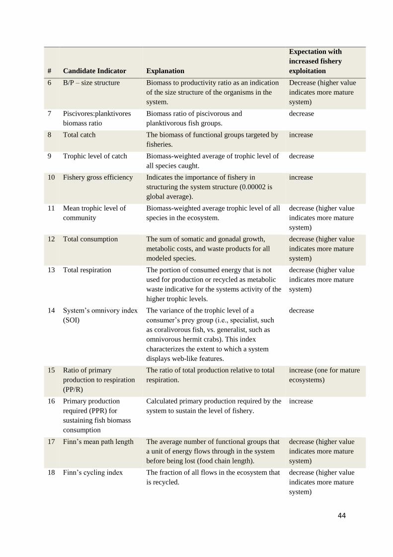
44
# Candidate Indicator Explanation
Expectation with
increased fishery
exploitation
6 B/P – size structure Biomass to productivity ratio as an indication
of the size structure of the organisms in the
system.
Decrease (higher value
indicates more mature
system)
7 Piscivores:planktivores
biomass ratio
Biomass ratio of piscivorous and
planktivorous fish groups.
decrease
8 Total catch The biomass of functional groups targeted by
fisheries.
increase
9 Trophic level of catch Biomass-weighted average of trophic level of
all species caught.
decrease
10 Fishery gross efficiency Indicates the importance of fishery in
structuring the system structure (0.00002 is
global average).
increase
11 Mean trophic level of
community
Biomass-weighted average trophic level of all
species in the ecosystem.
decrease (higher value
indicates more mature
system)
12 Total consumption The sum of somatic and gonadal growth,
metabolic costs, and waste products for all
modeled species.
decrease (higher value
indicates more mature
system)
13 Total respiration The portion of consumed energy that is not
used for production or recycled as metabolic
waste indicative for the systems activity of the
higher trophic levels.
decrease (higher value
indicates more mature
system)
14 System’s omnivory index
(SOI)
The variance of the trophic level of a
consumer’s prey group (i.e., specialist, such
as coralivorous fish, vs. generalist, such as
omnivorous hermit crabs). This index
characterizes the extent to which a system
displays web-like features.
decrease
15 Ratio of primary
production to respiration
(PP/R)
The ratio of total production relative to total
respiration.
increase (one for mature
ecosystems)
16 Primary production
required (PPR) for
sustaining fish biomass
consumption
Calculated primary production required by the
system to sustain the level of fishery.
increase
17 Finn’s mean path length The average number of functional groups that
a unit of energy flows through in the system
before being lost (food chain length).
decrease (higher value
indicates more mature
system)
18 Finn’s cycling index The fraction of all flows in the ecosystem that
is recycled.
decrease (higher value
indicates more mature
system)

45
# Candidate Indicator Explanation
Expectation with
increased fishery
exploitation
19 Predator cycling index The fraction of all flows in the ecosystem
recycled through non-detrital pathways
indicates the importance of predation in the
structure and functioning of the system at
higher trophic levels.
decrease
20 Total system throughput
(TST)
Represents all of the biomass flows and is the
summation of consumption, respiration,
export and flows to detritus.
decrease (higher value
indicates more mature
system)
21 Capacity Measurement of size and complexity of the
system, calculated as the product of TST and
the maximum degree of specialization.
decrease (higher value
indicates more mature
system)
3.3 Results
3.3.1 Model structure and sensitivity
The Hawai`i Ecopath models’ pedigree index values were 0.50 for FFS, 0.59 for O`ahu and
0.62 for Kona; all values fell in the medium–high range compared to 50 other Ecopath
models, 48% of which had a pedigree from 0.40 to 0.59 and only 10% of which had a
pedigree higher than 0.60 (Morissette 2007). These results suggest that the model is well
rooted in local data and, therefore, robust.
Sensitivity analyses showed that the model was least sensitive to a change in Q/B
ratio for the meiobenthos (e.g., benthic filter feeders, benthic carnivores, benthic deposit
feeders and crustaceans), with only crustacean biomass changing more than 10% with a 50%
applied increase or decrease of their Q/B ratio. However, decreasing the Q/B by 50% resulted
in an unrealistically ratio of production over consumption (P/Q) of > 1 for benthic filter
feeders. Benthic carnivores were the least sensitive group to changes in P/B ratio compared to
the other small invertebrate groups (Fig. 3.2). Exploration of the sensitivity of the Q/B ratio
with a decreasing biomass or P/B ratio (–25% and –50%) resulted in failure of the Ecopath
model to calculate the EE. In comparison, elevation of these values resulted in a very high
increase in the Q/B ratio, especially for benthic filter feeders as a response to a biomass
increase and for benthic detritivores as a response to a P/B ratio increase. P/Q ratio values
were unrealistically low (< 0.05) for all groups when biomass was changed and for all groups
except the benthic carnivores when P/B changed. In contrast, biomass and the P/B ratio were
not very sensitive to increasing P/B ratio or biomass, respectively, but more so to decreasing
those values except for the biomass of benthic carnivores. Clearly, more study needs to be
devoted to these invertebrate groups to obtain a better estimate of their biomass and P/B ratio
for model improvement.

46
Figure 3.2. Results of sensitivity analysis of four invertebrate groups to changing the P/B ratio on the
biomass. CRS=corals, BFF=benthic filter feeders, BD=benthic detritivores, BC=benthic carnivores.
3.3.2 General description of the three systems
Ecopath aggregates an entire system into distinct trophic levels sensu Lindeman (Christensen
et al. 2008). FFS showed a higher overall biomass with the main differences in the higher
trophic groups (Fig. 3.3). The models estimated that the majority (57%–64%) of the energy
flows originated from detritus rather than from primary productivity, indicating that
secondary production is based mainly on detritus and net primary production enters the coral
reef food chain through heterotrophic benthic organisms. Transfer efficiency was highest
from trophic level I to II, especially for the energy flow from detritus, suggesting high energy
efficiency at the lower trophic levels. Although the total biomass values for the Kona system
and the FFS system were similar, the transfer efficiency for the higher trophic levels (5 and
up) was 1.5 to 2.5 times higher in FFS compared to both O`ahu and Kona. The importance of
detritus and high efficiency in recycling also was corroborated by the high values for Finn’s
cycling index, especially in the models with no (FFS) or intermediate (Kona) fishing
perturbation.
Figure 3.3. Composition of biomass (t/km2) per trophic level (TL) for the three systems studied in
Hawai`i. FFS is French Frigate Shoals; Kona represents the Kona Coast of Big Island.

47
3.3.3 Evaluation of indicators based on analyses of survey data
Benthic indicators derived by field surveys did not show any clear relationship with fishing
pressure (Table 3.3); thus, habitat parameters alone cannot be used as fishery indicators.
However, fish indicators did reflect the fishing pressure gradient. Direct effects of fishing
were reflected in the increase in total catch and decrease in biomass of apex predators (roving
piscivores and sharks) and of large-sized (≥ 50 cm) fishes with increasing fishing pressure
(Table 3.3). Also, total fish biomass showed high values at FFS, intermediate values at Kona,
and low values at the most populated (highest fishing pressure) island of O`ahu. The disparity
in biomass of large fishes and apex predators between FFS and Kona is noteworthy in that it
is much greater than the disparity between Kona and O`ahu, indicating that these indicators
are quite crude and that the effect of fishing is almost binary (populated/unpopulated).
Against expectations, results show that biomass of planktivores (e.g., Melichthys
niger, Naso hexacanthus, Myripristis sp., Chromis sp.) strongly declined with an increase in
fishing pressure (Table 3.3). Planktivorous fishes are mostly prey fishes, and their biomass
was expected to go up with a release of predation pressure (Fulton et al. 2005).
Table 3.3. Benthic (B) and fish (F) related indicators for coral reef health from survey data
(unnumbered; NOAA Fisheries Coral Reef Ecosystem Division and Hawai`i Department of Aquatic
Resources indicators) and candidate indicators (numbered) for fishery effects. The numbers
correspond to the numbers in Table 3.2 for details on these indicators. Standard error given in
parenthesis. FFS is French Frigate Shoals; Kona is the Kona Coast of Big Island.
No B/F (Candidate) Indicators FFS Kona O`ahu
B Total biomass benthic algae (g/m2) 281 225 307
B Total cover macroalgae (%) 12.5 (6.44) 2.3 (0.92) 17.7 (2.24)
B Total cover crustose coralline algae (%) 8.0 (5.01) 8.9 (0.94) 6.8 (0.88)
B Coral cover (%) 20.3 (6.61) 24.6 11.3 (1.36)
B Habitat complexity (towed-diver surveys
2008–2010; 1 is low, 5 is high) 2.2 2.9 1.9
F Total fish biomass (Rapid Ecosystem
Assessment surveys 2005–2010) (g/m2) 92 68 20
F Large (≥ 50 cm) fish biomass (towed-
diver surveys 2006–2010) (g/m2) 6.9 1.4 0.8
4 F Biomass apex predators (sharks and
roving piscivores) (g/m2) 4.86 0.30 0.26
5 F Biomass planktivores (g/m2) 19.09 12.94 4.50
6 F Piscivores:planktivores biomass ratio
(g/m2) 0.33 0.52 0.23
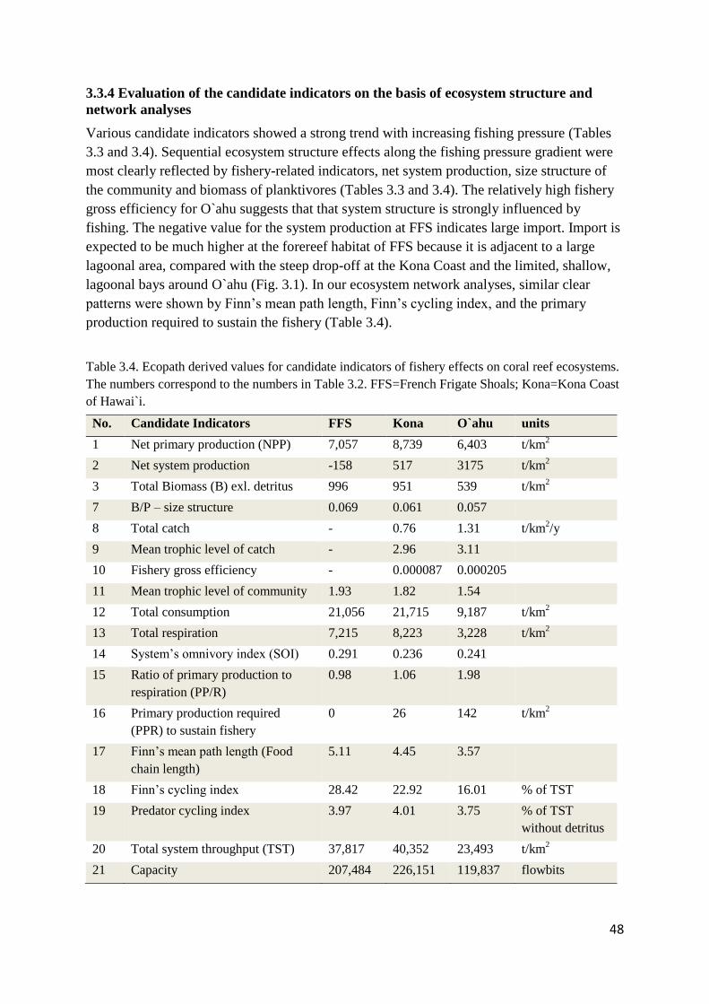
48
3.3.4 Evaluation of the candidate indicators on the basis of ecosystem structure and
network analyses
Various candidate indicators showed a strong trend with increasing fishing pressure (Tables
3.3 and 3.4). Sequential ecosystem structure effects along the fishing pressure gradient were
most clearly reflected by fishery-related indicators, net system production, size structure of
the community and biomass of planktivores (Tables 3.3 and 3.4). The relatively high fishery
gross efficiency for O`ahu suggests that that system structure is strongly influenced by
fishing. The negative value for the system production at FFS indicates large import. Import is
expected to be much higher at the forereef habitat of FFS because it is adjacent to a large
lagoonal area, compared with the steep drop-off at the Kona Coast and the limited, shallow,
lagoonal bays around O`ahu (Fig. 3.1). In our ecosystem network analyses, similar clear
patterns were shown by Finn’s mean path length, Finn’s cycling index, and the primary
production required to sustain the fishery (Table 3.4).
Table 3.4. Ecopath derived values for candidate indicators of fishery effects on coral reef ecosystems.
The numbers correspond to the numbers in Table 3.2. FFS=French Frigate Shoals; Kona=Kona Coast
of Hawai`i.
No. Candidate Indicators FFS Kona O`ahu units
1 Net primary production (NPP) 7,057 8,739 6,403 t/km2
2 Net system production -158 517 3175 t/km2
3 Total Biomass (B) exl. detritus 996 951 539 t/km2
7 B/P – size structure 0.069 0.061 0.057
8 Total catch - 0.76 1.31 t/km2/y
9 Mean trophic level of catch - 2.96 3.11
10 Fishery gross efficiency - 0.000087 0.000205
11 Mean trophic level of community 1.93 1.82 1.54
12 Total consumption 21,056 21,715 9,187 t/km2
13 Total respiration 7,215 8,223 3,228 t/km2
14 System’s omnivory index (SOI) 0.291 0.236 0.241
15 Ratio of primary production to
respiration (PP/R)
0.98 1.06 1.98
16 Primary production required
(PPR) to sustain fishery
0 26 142 t/km2
17 Finn’s mean path length (Food
chain length)
5.11 4.45 3.57
18 Finn’s cycling index 28.42 22.92 16.01 % of TST
19 Predator cycling index 3.97 4.01 3.75 % of TST
without detritus
20 Total system throughput (TST) 37,817 40,352 23,493 t/km2
21 Capacity 207,484 226,151 119,837 flowbits

49
The remaining candidate indicators did not show a clear sequential pattern with
increases in fishing pressure, but many indicators pertaining to the system’s stability or
maturity sensu Odum (1969) showed a binary pattern, with a minimal difference between
FFS and Kona (Table 3.4). For example, mature, stable systems have a close coupling
between production and respiration (P/R ~ 1) and, therefore, have no or little excess
production, a high system throughput and capacity and high overall biomass. Other indicators
that showed the same binary pattern were total biomass, mean trophic level of the community
and biomass of roving piscivores. On the basis of the indicators for system maturity (Table
3.4), it appears that the reef system around O`ahu is in a more transitional state compared to
the reef systems around FFS and along the Kona Coast. This difference could be a result of
higher fishing perturbations as habitat (benthic indicators) did not show this trend.
Candidate indicators that did not show a simple linear pattern with an increase in
fishing pressure were the piscivore:planktivore ratio and the net primary production. The
system’s omnivory index showed minimal to no differences among the three systems,
indicating that the complexity of the food webs was similar. The trophic level of the catch
was also similar between Kona and O`ahu.
3.4 Discussion
The results should be regarded as trends as it is impossible to make rigorous statements on
the basis of only three points. Ideally, more Ecopath models will be developed for other
islands in the Hawaiian Archipelago to get a better understanding of which combination of
variables are most indicative for fishing pressure.
3.4.1 Model structure and sensitivity
In coral reefs, roughly 50% of the net primary production (NPP) produced offshore and on
the reefs is channeled through the microbial loop (Azam et al. 1983, Pernthaler 2005, Zöllner
et al. 2009). This high efficiency in reefs was successfully simulated in the model on the basis
of the high detritus dependence and the high value of Finn’s cycling index, especially for the
Kona and FFS models. Including the microbial food web in the model increased total energy
throughput and energy transfer efficiency (TE) from detritus but decreased the TE from
primary productivity (PP). These effects could be caused by enhanced recycling of materials
and energy by the microbes; therefore, including the microbial loop simulates the system
behavior more appropriately (Paves and Gonzalez 2008). In all three models, TE was 1.4 to
1.8 times higher from detritus than from primary production, corroborating the importance of
the microbial loop in coral reef ecosystems. On the basis of the pedigree, it was clear that all
three models are highly rooted in local data enhancing the robustness.
Area is an important variable that influences model results. Comparison of our model
results with results from other regional models was difficult because study area, survey
methods and functional groups varied between models. The FFS Ecopath model of Parrish et
al. (2011) also has a shallow (0–30 m) reef component, and, when comparable areas were
derived, the fish biomass in Parrish et al’s model was 94.3 g/m2, which compared very well
with our 91.6 g/m2. It was not possible to compare any other functional groups. A Kona coast
model (Wabnitz unpubl. data) includes the same shallow reef area that was used in this study

50
but extends to a depth of 100 m and includes all habitat types for a total study area of 90 km2.
In our study, we only used the forereef area at depths of 0–30 m for a total area of 68 km2.
Wabnitz (unpubl. data) used shallow (0–30 m) fish biomass values from Friedlander et al.
(2006), and our estimate of 67.7 t/km2 for our Kona coast model is very comparable with
their hard-bottom estimates (ranging between 40 and 85 t/km2) for their four Kona sites. We
feel, therefore, confident that our fish biomass numbers are realistic.
The lower trophic groups have been considered mostly as biomass pools in other
reported reef models and are the groups of greatest uncertainty; hence, variation can be
expected. Urchin biomass in this study was 19 t/km2, which was 5 times lower than values
from Wabnitz (unpubl. data). Another discrepancy between Wabnitz (unpubl. data) and this
study was the biomass of corals. Coral biomass in this study adjusted for the sand habitat (no
corals) was 194 t/km2 and in Wabnitz et al. 82 t/km
2. This large difference in coral biomass
could be caused by the (assumingly) low coral cover in the mesophotic depth included in the
Wabnitz (unpubl. data) study area. Clearly, more research on invertebrates would greatly
enhance the model. Sensitivity analyses of the meiobenthos showed that changes in the Q/B
ratio had little effect on the biomass or P/B ratio, but decreasing the biomass by 50% resulted
in a change in P/B of 80%–100% for all four invertebrate groups and decreasing the P/B ratio
resulted in a change in biomass of 100% for benthic filter feeders and deposit feeders and
136% for crustaceans. Our biomass estimates for these groups came from studies of the Kona
Coast of Hawai`i supplemented by visual observations at hard-bottom sites in each system,
and the P/B (and Q/B) ratios were weighted according to the species composition at each
system and are in the range of values reported in other reef systems (Weijerman et al. 2013).
Because these lower trophic functional groups play an important role in the transfer
efficiency of energy, better estimates are highly recommended to improve the model.
3.4.2 Evaluation of indicators derived by monitoring programs
Coral and macroalgal cover are variables that are widely used as metrics in evaluating reef
health and are also included in DAR’s monitoring program and the Pacific RAMP. Solely on
the basis of these habitat indicators, reefs along the Kona Coast of Hawai`i (intermediate
fishing) would be categorized as being in a better health than are reefs in FFS (no fishing;
Table 3.3). Therefore, these variables are not directly indicative for fishery effects. Fishing
does not necessarily degrade reefs, high macroalgal cover does not necessarily indicate a
degraded reef (Parrish and Boland 2004, Vroom and Braun 2010) and high coral cover does
not necessarily indicate a reef with high fishable biomass (McClanahan et al. 2011a).
In contrast, large-fish biomass and the candidate indicator, biomass of apex predators,
showed a strong relation with fishing pressure; albeit, not a sequential relation, it was more a
binary pattern where intermediate fishing pressure resulted in a sharp decline in biomass of
these species. The piscivore:planktivore ratio was one of the indicators that was most robust
in other system studies (Fulton et al. 2005) but was not an effective indicator of fishing
pressure on the Hawaiian reef systems. This result could be because the biomass estimates for
apex predators from towed-diver surveys were used. If biomass estimates from REA (small-
scale) surveys were used, the piscivore:planktivore ratio would be 3.34 for FFS, 0.52 for
Kona, and 0.19 for O`ahu, where shark and jack encounters in REA surveys are rare. This

51
deceasing trend is what you would expect along a gradient of increasing fishing mortality
with target species declining and planktivorous species contributing a larger part to fish
assemblages (Fulton et al. 2005). However, in fished areas, jacks and sharks are likely wary
of divers and swim away, and their numbers can be underestimated; whereas, in protected
areas (such as FFS), jacks and sharks might be more curious and approach divers, hence, their
numbers are likely to be overestimated at REA sites. Therefore, the biomass estimates from
towed-diver surveys are believed to be more accurate (Richards et al. 2011). The same holds
true for the biomass of planktivores, which, against expectations, decreased with increasing
fishing pressure. This phenomenon could be explained by fishing mortality; according to the
Hawai`i fishery statistics, planktivorous soldierfishes (Myripristis sp.), unicorn fish (Naso
breviosis) and some sergeant fishes (Abudefduf sp.) are targeted in the fishery and could drive
their numbers down in the populated areas. Although the exact drivers of this phenomenon
are unknown, this trend of high planktivorous biomass in remote areas compared to populated
areas also is observed elsewhere in the Pacific (Williams et al. 2011).
3.4.4 Evaluation of candidate indicators derived by Ecopath
Evaluation of the candidate indicators across a fishing pressure gradient showed that
indicators at the community level were most robust (i.e., clearest trend) and that multiple
indicators are necessary to identify fishing perturbation. Candidate indicators related to the
system’s community, such as total biomass, community size structure and trophic level of the
community, were indicative of fishing pressure and could be used as performance indicators
compared to a baseline (e.g., a 1950 system).
Community and ecosystem attributes deal with energy flows and ecosystem
functioning and are not readily measurable from field studies. Throughput, production, and
consumption—along with the internal state (i.e., Finn’s cycling index, mean path length)—
reflect a system’s ability to support its current state and level of exploitation in the long term
(Vasconcellos et al. 1997, Fulton et al. 2005). On the basis of the statistics of metrics
indicative of a system’s maturity sensu Odum (1969), reefs around FFS and along the Kona
Coast were in a stable, mature state and the observed level of fishing along the Kona Coast
was supported by the system. However, the coral reef ecosystem around O`ahu appears to be
in a transitional state and fishing mortality is assumed to have played an important role in the
current structure and functioning of this ecosystem. The mean trophic level of the community
was an indicator that showed a clear decreasing trend with an increase in fishing pressure
across the three study areas as did the biomass/production ratio, the mean food chain length
and Finn’s cycling index. The low EE for benthic algae (0.16–0.33) indicates a lack of
herbivorous grazing pressure that could drive the transitional state (i.e., moving from a coral
dominated system to an algal dominated system). Results from 7 out of 10 long-term (> 10
year) monitoring programs in O`ahu showed a coral cover decline of 4% to 35%,
corroborating this hypothesis (Friedlander et al. 2008). Naturally, fishing mortality is not the
only perturbation that affects the status of coral reef ecosystems. We used human population
as an indicator for fishing intensity; however, with an increased population, other stressors to
reef ecosystems, such as sedimentation, nitrification, and other land-based sources of
pollution, also augment. Notwithstanding, the results from the Ecopath models in our study

52
do show that fishing-related indicators did indicate a clear decreasing trend with an increase
in fishing mortality and benthic indicators did not.
3.5 Conclusions
Candidate indicators for fishing pressure showed that indicators at the community level (e.g.,
total biomass, community size structure, trophic level of the community) showed the clearest
trend with increased fishing mortality. Results also showed that multiple indicators are
necessary to identify fishing perturbations. These indicators could be used as performance
indicators when compared to a baseline for management purposes. Currently, collected data
from monitoring programs in Hawai`i of fish biomass and fish assemblages and size structure
clearly show a strong relation to fishing mortality, with higher fishing mortalities resulting in
a shift in fish communities (decrease in number of large fishes and in biomass of piscivores),
unlike data of benthic parameters (e.g., coral or algal cover). Ecopath statistics of the
structure and functioning of ecosystems can supplement these metrics with insights into the
stability of the system. Stable, mature systems are more likely to recover from perturbations,
such as global change or local stressors to reefs (e.g., land-based sources of pollution,
fishing). Understanding the processes that structure a reef is important in supporting marine
resource managers to reverse transitional states to stable systems that yield high fishable
biomass. On the basis of the results of this study, it is clear that the reefs around O`ahu are in
a transitional state. The low EE for benthic algae around O`ahu, compared to around Kona
and FFS, indicates that grazing pressure was minimal. Reduced grazing of (especially)
macroalgae by herbivores could result in a shift to a system that is dominated by algae instead
of corals; the latter is economically and aesthetically more desirable as it supports a higher
fishable biomass and dive tourism. In follow-up studies, it would be beneficial to use Ecosim,
a simulation model that uses Ecopath for input parameters, to evaluate management scenarios
that are most likely to succeed in reversing the current transitional state of the coral reefs
around O`ahu.

53
Branching Acropora coral. Photo Dave Burdick

54
Chapter 4
Design and parametrization of a coral reef
ecosystem model for Guam
Weijerman, M, IC Kaplan, EA Fulton, R Gorten, S Grafeld, and R Brainard. 2014. Design
and parameterization of a coral reef ecosystem model for Guam. U.S. Dep. Commer., NOAA
Tech. Memo., NOAA-TM-NMFS-PIFSC-43. 133 + Appendices

55
Declines in the fish stocks and degradation of habitats around Guam have
serious implications for the residents of Guam who depend on the ecosystem
services provided by coral reefs. Management on an ecosystem scale has
proven to be a useful strategy to conserve, manage and restore marine
systems. Implementing ecosystem-based management requires an
understanding of the complex and often synergistic dynamics of coral reefs,
including the role of humans in the ecosystem. The Atlantis modelling
framework integrates physical, biogeochemical, ecological, and
anthropogenic processes in a three-dimensional, spatially explicit domain and
can serve as an useful decision-support tool for ecosystem-based coral reef
management. We describe the details of each model component and present
the parameterizations of the spatial and ecological modules in Atlantis.
The Guam Atlantis model is focused on the shallow (< 30 m) coral
reefs fringing Guam and is predominantly based on biological data collected
in Guam. The Atlantis model uses polygons as its ‘grids’ which were drawn to
represent areas of similar ecological and oceanographic characteristics while
also taking into account the spatial strata of fisheries catch data and existing
spatial management areas. In the ecological module food-web dynamics of 42
functional groups are simulated: 3 detritus, 2 bacteria, 5 plankton, 3 algae, 2
corals, 7 invertebrate, and 20 vertebrate groups. We gathered and analyzed
environmental, habitat, biological, and fishery data from diverse sources.
These data helped us identify information gaps, such as, near-shore habitat
data, biomass and abundance data of invertebrate species, chlorophyll-a data
at different depths and certain life history parameters for invertebrates and
fish.
After calibration and testing we believe that the model produces an
adequate representation of Guam’s coral reef ecosystems. However, there still
is a need for the incorporation of coral-reef-specific dynamics and improved
physical oceanography to better simulate coral reef processes around Guam.
These aspects are described in Chapter six.

56
4.1 Introduction
Coral reef ecosystems are important as habitats, natural buffers, sites for recreation and
cultural practices and as a key component of the marine economy. Coral reefs generate
millions annually from marine tourism (Cesar et al. 2003, Van Beukering et al. 2007) and are
important to the social and economic welfare of coastal communities (Moberg and Folke
1999). Commercial and recreational fisheries support many jobs and fishing expenditures
generate millions of dollars in sales revenues and value-added benefits. Furthermore, in many
Pacific islands, fisheries serve vital non-market functions, such as building social and
community networks, perpetuating fishing traditions and providing fish to local communities.
Yet, compared to pelagic fisheries, reef-associated fisheries have received little attention
(Sadovy 2005). However, it is well established that there is a positive feedback between coral
cover and reef-fish biomass (Jones et al. 2004, Green et al. 2009). When reef-building corals
are lost, the subsequent reduction in structural complexity results in reduced species diversity
and a loss of fish species that fulfill important ecological roles in the resilience of coral reefs
(Jones et al. 2004, Graham et al. 2006, Alvarez-Filip et al. 2009). There is a general
consensus among scientists that coral reefs are in trouble (Bruno and Selig 2007, Carpenter et
al. 2008, Wilkinson 2008). In recent reviews on the extinction risks of corals, two of the most
important threats to the survival of corals and especially coral reefs were identified as being
human-induced ocean warming and ocean acidification (Brainard et al. 2011, Burke et al.
2011).
Massive and branching stony corals are the primary framework builders and a major
source of calcium carbonate production of coral reefs. Two main processes regulate the
abundance or growth of corals and other calcifiers: (1) accretion determined by the narrow
range of suitable environmental conditions that allows the deposition of calcium carbonate,
and (2) erosion resulting from physical, chemical, and biological processes. Reef structures
are built by combining calcium and carbonate ions derived from the seawater into aragonite
(or calcite) crystals that form the corals’ skeletons. These coral skeletons and crustose-
coralline algae are often cemented together with aragonite and high-magnesium calcite to
form reefs. Natural ongoing bioeroding processes of this carbonate substrate influence the net
structural growth (Perry et al. 2012). It is ultimately the maintenance of these three-
dimensional structures rather than the corals themselves that provide the reef’s functions and
ecosystem services (Graham et al. 2006, Perry et al. 2012).
Reef accretion requires energy and if the external aragonite or calcite saturation states
decrease as a result of increased atmospheric CO2, calcification will reduce or stop altogether
(Langdon and Atkinson 2005). Atmospheric CO2 has increased rapidly from its pre-industrial
level of 280 ppm to over 400 ppm today and the earth’s system has already warmed, on
average, close to 0.74°C globally over the last century primarily as a result of greenhouse gas
emissions (IPCC 2007). Elevated water temperature can lead to coral bleaching (the
expulsion of symbionts that give corals their color) and disease epizootics and have already
resulted in repeated mass coral bleaching and mortality events worldwide (reviewed in
Brainard et al. 2011). Current projections on global increases in atmospheric carbon dioxide
concentrations, water temperatures and ocean acidification have led to predictions of a
significant loss of corals and other calcifying marine organisms, resulting in reduced diversity

57
of reef communities and a reduced resilience of corals to local stressors (Hoegh-Guldberg et
al. 2007, Kennedy et al. 2013).
While local governments are limited in their capacity to reduce greenhouse gas
emissions and so reduce the ongoing ocean warming and acidification, they can play a pivotal
role in enhancing the corals’ capability to recover from impacts of these global threats by
reducing additional local stressors caused by land-based sources of pollution and excessive
fishing (Carilli et al. 2009, Hughes et al. 2010, Kennedy et al. 2013). Based on their high
biological diversity, coral reef ecosystems likely have increased functional redundancy,
which is expected to provide increased resilience (resilience defined as the capacity to
‘bounce’ back from a disturbance) compared with less-diverse ecosystems. However, this
capacity of organisms and natural systems to bounce back can by degraded by sequential,
chronic, and multiple disturbances, physiological stress and general environmental
deterioration (Nyström et al. 2000). Loss of resilience may take many forms, including
increased disease susceptibility, impaired reproduction and recruitment, loss of functional
diversity/redundancy in communities and reduced individual growth rates.
A critical part of any local management approach to enhance coral recovery from
global threats is the mitigation of local stressors that affect coral-macroalga competition,
early life history development and coral survival (Baskett et al. 2009b, Gilmour et al. 2013).
This approach can be met through the protection of a large and diverse herbivorous fish
population (Pandolfi et al. 2003, Bellwood et al. 2006) and through the reduction of nutrient
input which favors algal growth above coral growth (Fabricius 2005). While some reefs are
still in fair to good condition, many near-shore ecosystems adjacent to urban areas and
popular destinations have suffered from land-based sources of pollution, fishing pressure,
recreational overuse, crown-of-thorns seastar outbreaks and ocean warming (Wilkinson
2008).
As reefs provide a wealth of benefits to adjacent local communities, protecting these
reefs from deterioration is a major endeavor for governments. Limits to fishing through the
degradation of fish habitat, declines in important fish populations or increased regulations
have the potential for important cultural, economic, and social implications to the residents of
near-shore communities. Despite the importance of reefs and near-shore habitats to Guam’s
economy and culture, the condition of marine resources has generally degraded over the past
20 years (Burdick et al. 2008, Richmond et al. 2008). In recent years, additional development
and construction have begun to accommodate the translocation of about 40,000–60,000
military personnel and civilians (Kan 2013). Naturally, this new infrastructure will likely
result in increases in impermeable surfaces, demand on wastewater treatment and solid waste
facilities, and use of marine resources.
Effective local management must be based on proper understanding of coral reefs as
ecosystems and of the complex and sometimes synergistic impacts of different stressors while
also taking into account social and economic dependencies on these marine resources. As a
first step, resource managers and users can benefit from forecasts of the ecological, economic
and social impacts of alternative management strategies and of an increase in human
population. Secondly, state and federal agencies have specific mandates to choose actions to
mitigate impacts on coastal ecosystems and economies. For example, NOAA Fisheries plays

58
a supportive and advisory role in the management of living marine resources in coastal areas
of Guam, and ecosystem-based management is an important component of NOAA’s Habitat
Blueprint Initiative (http://www.habitat.noaa.gov/habitatblueprint/) and Next Generation
Strategic Plan (http://www.ppi.noaa.gov/ngsp/), as well as in the U.S. National Ocean Policy
2010 (http://www.doi.gov/pmb/ocean/policy/index.cfm). To date, however, few tools have
been available to support effective implementation of ecosystem-based management.
Models, as simplistic representations of ecosystems, can serve as useful tools to
support decision making. Coral reefs models have been developed to investigate various
aspects of the ecology of coral reefs with or without the predicted effects of global change,
such as erosion and accretion (Eakin 1996, Kennedy et al. 2013), coral growth (Hoeke et al.
2011), larval connectivity (Mumby et al. 2011), space competition (Mumby 2006), influence
of light on coral growth (Kleypas 1997), existence of alternative stable states (Żychaluk et al.
2012), effects of environmental perturbations on benthic community dynamics (Kubicek et
al. 2012), and evaluation of management strategies that would improve reef resilience mostly
focusing on fishing regulations (Mumby 2006, Edwards et al. 2011, Melbourne-Thomas et al.
2011a). One model that integrates various disciplines and addresses agency mandates is the
Atlantis Ecosystem Model (Atlantis) developed by Dr. Elizabeth Fulton at the
Commonwealth Scientific and Industrial Research Organisation (CSIRO), Marine and
Atmospheric Research in Hobart, Australia1 and can simulate the complex ecosystem
processes that link the physical environment with the associated biological and human
communities (Fulton 2001, Fulton et al. 2004a, Fulton et al. 2004c). It also includes the main
steps in an adaptive management cycle (including feedback from resource managers on
performance indicators) and can be used as a decision-support tool allowing for the
evaluation of ecological and economical cost-benefits of alternative management strategies.
A 2007 United Nations Food and Agriculture Organization report, which reviewed the
world’s leading 20 ecosystem-modelling platforms, rated CSIRO's Atlantis ecosystem
model as the best in the world for evaluating management strategies at an ecosystem level
(Plagányi 2007). However, to date the Atlantis framework has not been developed for a
coral reef ecosystem so this approach, outlined in this chapter and chapter six, will be
novel.
4.1.1 Stakeholder Participation
A requirement for effective ecosystem-based management is that local and federal
stakeholders and resource managers identify and agree on common goals and objectives,
such as clean water, sustainable coastal habitats and fisheries and conservation of
biodiversity. To measure progress towards these agreed-upon goals, identifiable ecological
and socioeconomic indicators need to be established. In November 2012, a workshop was
held in Guam where local and federal resource managers, scientists, the fisheries
cooperative, nongovernmental organizations and the Navy were invited to participate
(Weijerman and Brown 2013). That workshop resulted in the common goal to identify
management strategies that would reverse the downward trend in coral cover and fish
biomass and mitigate the effects of the expected increase in human population associated
1 http://atlantis.cmar.csiro.au/

59
with the military build-up. Ecosystem attributes were identified as “having a sustainable coral
reef ecosystem that can recover from the current local (e.g., fishery, land-based sources of
pollution, crown-of-thorns seastar predation) and global (ocean acidification and warming)
threats” (Weijerman and Brown 2013). Additionally, ecological and socioeconomic
indicators to track progress and management scenarios were identified so that model
simulations could help understand the tradeoffs among ecosystem services of the alternative
scenarios. These management scenarios were further developed in a follow-up workshop in
June 2014.
4.1.2 Objective
In this chapter, we present the basic formulations and parameterization of the Guam
Atlantis Model. We describe the spatial delineation of the model extent, the aggregations of
species into functional groups and the data processes and sources used for all biological
parameterizations. Additionally, we describe the physical forcing files that are used in the
model and briefly mention the fishery characteristics of Guam. We intend to apply the
model to explore ecological and socioeconomic tradeoffs of the identified alternative
management scenarios once the model is fully developed (Chapters seven and eight). At
this stage we have initialized the model to represent the present day (2011) ecosystem
status of Guam’s reefs, to (1) simulate the expected shift to a quasi-equilibrium state of a
reef system assuming an absence of human stressors or natural disturbances; and (2)
examine the modeled response to a range of fishing mortalities.
4.2 Guam
A summary overview of Guam is given here but for more detailed information see e.g.,
Burdick et al. 2008, Richmond et al. 2008, Brainard et al. 2012.
Guam is one of the largest and most populated islands in Micronesia with a total
land area of 544 km2 and a coastline of 244 km. It is about 48 km long and between 6 and
19 km wide. Guam is located at the southern tip of the Mariana Archipelago at 13°28’ N
and 144°45’ E. The nearest island in the archipelago is Rota which is part of the
Commonwealth of the Northern Mariana Islands (CNMI) located 60 km northeast of Guam
and the Philippines located 2,568 km west of Guam. Guam’s population is around 160,000
(U.S. Census 2010) and it is a popular tourist destination with around 800,000 visitors
every year mainly concentrated in Tumon Bay on the west coast (Brainard et al. 2012).
Guam’s population is expected to increase with another roughly 60,000 people as a result of
the planned relocation of U.S. military personnel, their dependents, and support staff (Kan
2013). Major population centers are in Tumon Bay, the capital Hagåtña, and between
Tumon Bay and Anderson Air Force Base in the north (Fig. 4.1).

60
Figure 4.1. Location of Guam in the Mariana Archipelago (inset) and land cover of Guam showing
the main population centers in the central part of Guam, restricted access areas (military land), the
many rivers in the southern part of Guam, and five marine protected areas.
The northern part of Guam is relatively flat and primarily comprised of uplifted
limestone whereas the southern part is of volcanic origin with steep hills and over 40 rivers
draining into the coastal waters (Fig. 4.1). Guam has distinct wet and dry seasons with the
dry season extending from January to June and a mean rainfall of 79 cm (SD 42), and a wet
season from July to December with a mean rainfall of 176 cm (SD 25) (Lander and Guard
2003; Fig. 4.2). Humidity is around 80% and the mean air temperature is 28°C.

61
Figure 4.2. Mean monthly rainfall at five stations in Guam (1970–2000 data from Lander and Guard
2003). Anderson Airforce Base is in the North of Guam, the airport in the center, Hagåtña on the east
coat in the center of the island (see Fig. 4.1), Umatac is on the southwest coast and Ylig is on the
southeast coast just south of Hagåtña.
The major sea current influencing Guam is the North Equatorial Current bringing
oligotrophic waters to Guam (Suntsov and Domokos 2013). Oceanic primary productivity is
low around Guam compared to other islands in the Pacific especially compared to the Line
Islands close to the equator (Nadon et al. 2012; Fig. 4.3).
Figure 4.3. Oceanic primary productivity derived from satellite imagery (average from 1999–2009).
Figure taken with permission from Nadon et al. (2012).

62
Historically, Guam experiences many typhones. Guam’s typhoon season is during
the humid summer months and four major typhoons have impacted Guam since 1994
(Burdick et al. 2008). There has been a decrease in the number and intensity of typhoons in
the west Pacific in the past decade compared with earlier decades. Additionally, on average
every year three tropical storms pass Guam (Storlazzi et al. 2009b).
Various environmental and geological variables influence the structure and
composition of Guam’s reefs (Fig. 4.4).
Figure 4.4. Geological and environmental variables influencing Guam’s reef structure. Data from
NOAA Coral Reef Ecosystem Division, wave energy from Peter Houk, unpublished GIS layer.
Guam is surrounded by fringing reefs with some reef flats along the windward
areas. It is located close to the high-diversity region of the Coral Triangle and boasts more
than 5100 known marine species including more than 1000 nearshore fish species and more
than 375 species of stony, scleractinian corals (Paulay 2003). Fish biomass on Guam is low
compared with the unpopulated Northern Mariana Islands (Fig. 4.5).

63
Figure 4.5. Comparison of total fish biomass by consumer group around the islands in the Mariana
Archipelago related to human population size. The islands are represented from north to south ending
with Santa Rosa Bank (SRR), Guam is represented by the three letter code GUA. Data from CRED
surveys in 2003, 2005, 2007, and U.S. Census 2010.
Participation in reef fishery by the local population is seldom for economic reasons
but it plays an important role in strengthening social bonds and is a chief source of
enjoyment to Guam’s residents (Van Beukering et al. 2007). Fish catches and coral cover
have declined significantly over the last few decades. Small-scale fishery catches have
declined by 84% since 1950 (Zeller et al. 2007). Coral cover has decreased from 50% in the
1960s to 25% in the 1990 to 15% in 2010, a 70% decline in the last 50 years (Burdick et al.
2008, Brainard et al. 2012). The main threats to the corals of Guam are river run-offs
including heavy sediment loads that smother the corals in the southern reefs, ocean
warming that leads to bleaching often followed by coral mortality, crown-of-thorns seastar
outbreaks that can decimate coral populations and excessive fishing that leads to a
disruption of ecosystem processes. In response to these declines, the government of Guam
has created five marine preserves (MPAs; Fig. 4.1) and several watershed restoration
projects are underway. In 2011, fish biomass in the preserves was 2.4 times higher than in
the open areas around Guam (Williams et al. 2012). Additionally, the government of Guam
participates in the Micronesia Challenge which was launched in 2006.2 This initiative is a
commitment between Micronesian governments to balance between the need to use their
natural resources today and to sustain those resources for future generations. The five
Micronesian governments of the Republic of Palau, the Federated States of Micronesia, the
Republic of the Marshall Islands, the U.S. Territory of Guam, and the Commonwealth of the
2 http://www.micronesiachallenge.org/

64
Northern Mariana Islands all committed to “effectively conserve at least 30% of the near-
shore marine resources and 20% of the terrestrial resources across Micronesia by 20202.”
Guam’s population has almost tripled since 1960 increasing the pressure on natural
resources (Fig. 4.6). The population is likely to increase more steeply in the near future as a
result of the planned military buildup (Kan, 2013).
Figure 4.6. Population growth in Guam in the last decades (US Census) and future estimated growth.
The main source of terrigenous nutrient and sediment inputs in southern Guam is
through surface run-off and in northern Guam through underground seepage. Guam
sedimentation studies showed a sedimentation rate substantially higher than the amounts
determined to impact corals elsewhere (Pastorok and Bilyard 1985, Rogers 1990, Riegl and
Branch 1995, Te 2001, Scheman et al. 2002, Minton et al. 2006, Storlazzi et al. 2009a)
suggesting that the benthic community is under long-term pressure with potential gradual and
long-term declines and shifts in community structure. Sediments can smoother reefs, reduce
light in the water column, induce sublethal effects, impede fertilization and reduce
recruitment with the overall effect of reduced coral growth and shifts towards more
sediment–tolerant species assemblages depending on the duration and load of the
sedimentation (Richmond and Hunter 1990, Riegl and Branch 1995, Birkeland 1997,
Fabricius 2005). A primary effect of increased nutrients into the oligotrophic marine waters is
an increase in phytoplankton and benthic algae which are better in taking up these nutrients
and grow faster compared to corals (Lapointe 1997, Szmant 2002). Nutrients can impact
directly on coral physiology (increase zooxanthellae density) which disrupts the symbiosis
and affects metabolic processes, coral growth and reproductive success (Fabricius 2005) and
indirectly on space competition with other benthic organisms, such as filter feeders and algae
(Koop et al. 2001).
0
50
100
150
200
250
300
350
0
50
100
150
200
250
300
350
400
450
1950 1960 1970 1980 1990 2000 2010 2020 2030
Po
pu
lati
on
pe
r km
2
Po
pu
lati
on
x 1
00
0

65
4.3 Methods
4.3.1 Guam Atlantis Ecosystem Model
Atlantis model framework
The Atlantis framework was developed and refined in the early part of the 21st century
simulating the ecosystems of Port Phillip Bay and, later, the southeast open coast of
Australia. Atlantis is a three-dimensional, deterministic (differential equations), spatially-
explicit model based on nitrogen-flows through main trophic groups with primary processes
being consumption, production, migration, recruitment, waste production, and (natural and
fishing) mortality. The model incorporates spatially differentiated habitats (as polygons) and
vertical stratification (as water layers) allowing for the representation of hydrodynamic and
biological processes (e.g., vertical migration of fish to different habitat types in their
lifecycles, larval connectivity between reef areas). It incorporates a range of modules and
levels of detail that encompass most options for management actions available in coastal
waters. For instance, fishery options available at the fleet or species level include catch
quotas, gear restrictions, spatial closures, individual quotas, seasonal closures and effort
reductions. Nutrient/runoff management options include altering inputs of specific forms of
nitrogen or sediment concentrations in any model polygon. Model simulations can be used to
see if any of these scenarios consistently produce better outcomes in terms of improved
habitat and increased target fish stocks, productivity, and fecundity, over defined time periods
and to predict fisheries response to management of the fisheries.
Applications of Atlantis
Applications of Atlantis models have increased understanding of system dynamics; identified
major processes, drivers and responses; highlighted major gaps in knowledge; and provided a
mechanism to ‘road test’ management strategies before implementing them in reality (e.g.,
(Fulton et al. 2007, Kaplan et al. 2010, Griffith et al. 2011, Ainsworth et al. 2012). To date
Atlantis ecosystem models have been applied in Australia, the east and west coast of the
United States, the Gulf of Mexico, South Africa, and various models are in development in
Europe. One of the key findings from these applications is that there is no single management
application that provides a ‘silver bullet’ solution to ecosystem-based management (Fulton et
al. 2011b). Tradeoffs, especially between conservation and industry, are complex as
ecological, economic and social objectives vary greatly making it difficult to meet them all.
Another important finding is that because cumulative drivers are included in the application
of an Atlantis model, the resulting modifications in the ecosystem (e.g., water quality, habitat
suitability, productivity) can undermine or counteract the effects of fisheries management
(Fulton and Smith 2004, Kaplan et al. 2010, Fulton et al. 2014).
Limitations of Atlantis
As the Atlantis framework includes a wide range of complex options it can be tempting to use
them all resulting in a high spatial and trophic resolution. However, not placing emphasis on
the key dynamic processes and biological groups can lead to an unstable model that fails to

66
represent realistic trophic structures and ecosystem dynamics. At the other extreme, very low
spatial resolution or inappropriate trophic aggregation (e.g., across trophic roles) can lead to
misleading model behavior that also does not resemble reality. Because Atlantis includes so
many different data sets and processes, each associated with its own set of errors, Atlantis
should not be used for tactical management questions (e.g., fisheries stock assessments,
spatial allocation) but is more suitable for strategic direction settings in combination with
other model types. Another limitation of Atlantis and other complex end-to-end models is
handling uncertainty. Structural uncertainty can be explored (Fulton et al. 2003a, Fulton et al.
2004a, Fulton et al. 2004c) but uncertainty in parameters and data are more challenging, since
long simulation time preclude brute-force Monte Carlo approaches. Instead, these
uncertainties are handled by bounded parameterizations, multimodel inference and scenario
uncertainty (Fulton et al. 2011b). The strength of the Atlantis approach lies in ranking
different management actions based on defined objectives and potential scenarios for human
and ecological behavior, rather than in the estimation of statistical uncertainty.
Guam Atlantis Model development
In 2012, we began with the development of the Guam Atlantis Coral Reef Ecosystem Model
using the Atlantis framework. This approach is the first application of Atlantis to a coral reef
ecosystem. The first year was mainly to discuss the model objectives with stakeholders
(Weijerman and Brown, 2013) and collect and analyze the necessary data (Table 4.1). In
2013, we started with the parameterization of the spatial and ecological modules of Atlantis
(Fig. 4.7). The model’s start date is January 1, 2011 and this represents annual average
conditions. For some groups (e.g., roving piscivores, sharks, rays) with more limited data,
this date represents annual average conditions for approximately 2008–2011.
Figure 4.7. Schematic overview of the Atlantis framework and requirements for the spatial module
and resulting bgm file. BGM=box geometry.
Guam.bgm

67
Table 4.1. Summary of data streams used in the Guam Atlantis Coral Reef Ecosystem Model. Many
of these data are available as a GIS layer and available upon request from the first author. Fishery data
came from Guam Division of Aquatic and Wildlife Resources (DAWR) and NOAA’s Western Pacific
Fisheries Information Network (WestPacFIN).
Location Marianas, Guam
Oceanography Currents
Sea surface temperature (SST)
Waves
Chlorophyll-a
Near-shore
mapping
Bathymetry
Hard-soft bottom
Slope & Aspect
Rugosity
Habitat
Land cover &
anthropogenic
influences
Land cover
Roads
Population density
Watersheds
Streams
USGS flow rates and rainfall
Waste water treatment plants
Harbor (anthropogenic sites)
Injection wells
EPA water quality survey sites
Impaired water
Biological
data
Survey sites (DAWR, CRED)
Cryptic invertebrate species composition and abundance
Sea star and urchins biomass and spatial distribution
Pelagic bacteria sample sites & biomass
Coral, turf algae, macroalgae cover and biomass
Fish biomass (total biomass; size distribution, species composition, spatial
distribution)
Sea turtle numbers, biomass, and spatial distribution
Life history parameters, diet, migration, habitat dependency for all modeled groups
Fishery data Catch and effort statistics
Catch-per-unit-effort
Gear selectivity
Species composition of the catch
Reconstruction of fish biomass for 1985-2012
Dive preference study results
Spatial Model
The boundary of Guam Atlantis is the 30-m isobath with a total 0-30-m depth area of 95 km2
bordered by the coordinates: 13°39’ N, 144°57’ E, 13°14’ S, and 144°37’ W. Some coral-
reef- associated species are confined to hard substrate which is present in 73% of the total 0–
30 m area (e.g., coral, CCA, urchins, sea stars, corallivorous fish). Fish need a variety of
habitats and depth zones; shallow coastal habitat for recruit settlement and juvenile survival
and deeper habitats for foraging, sheltering and spawning sites for adults (Friedlander et al.
2007a, McMahon et al. 2012). These habitats include consolidated hard-bottom substrate
(live coral cover >10%) with low macroalgal cover (< 10%), high topographical complexity
(rugosity > 1.5 on a scale from 0 no rugosity to 5 high rugosity), access to unconsolidated

68
(sand) habitats and a wide range of depths (e.g., 0–30 m) (Friedlander and DeMartini 2002),
these habitats are included in the model.
Corals and marine species extend to below our 30-m model boundary. However,
available data are limited to safe diving depths of approximately 30 m for underwater survey
work. Notwithstanding, we believe that the population dynamics of the included marine
species are mostly within the model boundary. Home range studies show that most reef fish
have a strong site fidelity with movements of up to 1.6 km of coastline with continuous reef
and some degree of diel habitat shift (Meyer and Holland 2005, Meyer et al. 2010, Marshell
et al. 2011) although species can cross bare soft bottoms and travel over longer distances to
spawning aggregation sites or to establish a new home range (Chateau and Wantiez 2009).
The larger reef-associated piscivores also stay close (< 30 m) to the reef but roam
over larger areas with home ranges and mean distance from the reef increasing with fish size
and they show diel habitat shifts and movement to spawning aggregation sites during specific
times (Meyer et al. 2007, Afonso et al. 2009, Topping and Szedlmayer 2011). Only oceanic
plankton (including planktonic larval stages of coral reef species) and pelagic bacteria could
be exported out of our model boundary as they are influenced by the hydrology model as
passive drifters and are advected by currents.
Larval connectivity is difficult to estimate. Most models combine ocean current data
with a species’ life history characteristics to simulate larval dispersal from discrete habitat
patches in different seascapes (Cowen et al. 2006, Kool et al. 2011, Kendall et al. 2013).
Connectivity studies in the Indo-West Pacific showed that the oceanic conditions lead to a
transport of larvae from the South China Sea and from northern Papua New Guinea into the
Coral Triangle (Kool et al. 2011, Treml and Halpin 2012). The large-scale oceanic circulation
around Guam is controlled by the North Equatorial Current flowing northwestward
fluctuating in speed and direction (Fig. 4.8)3
(Bonjean and Lagerloef 2002). This
directionality could indicate that Guam is a stepping zone for larval dispersal from species
with a long pelagic larval duration from the outlying islands located southeast of the Mariana
Archipelago or from Papua New Guinea (Fig. 4.8). The nearest island Rota, at 60 km
northeast of Guam, could be another source of larvae. These potential larval supplies are
important for the development and maintenance of the biogeography, genetic variability and
biodiversity, however, it is likely less important for community recovery on short (< 50
years) time scales (Jones et al. 2009, Gilmour et al. 2013). Genetic studies show that marine
larvae are mostly retained within 20–30 km of their natal origin (Becker et al. 2007, Vollmer
and Palumbi 2007, Planes et al. 2009, Almany et al. 2013) which is supported by a near-
surface current study around Guam (Wolanski et al. 2003b). For larvae to find the right
microhabitat at the right time determines their success for establishment, i.e., lottery
hypothesis (Munday 2004a) (Geange and Stier 2009, Bode et al. 2011).
3 www.esr.org

69
Figure 4.8. Long-term (1993–2013) monthly mean large-scale oceanographic current patterns in the
west Pacific Ocean (Bonjean and Lagerloef 2002) for January (left) and August (right).
The coastal waters around Guam were divided into 55 polygons (Fig. 4.9). Polygon
delineations were based on similar characteristics (Fig. 4.4) of (1) the benthos defined by
NOAA National Ocean Service (NOS) Biogeography Branch (NOAA NCCOS 2005) and
updated by Guam Division of Aquatic and Wildlife Resources (DAWR) and CRED data; (2)
oceanographic conditions (CRED data; Peter Houk unpubl GIS layer); (3) bathymetry and
substrate type (CRED data); (4) existing protected areas (National Marine Protected Areas
Center)4 and (5) fishing use (Guam DWAR creel survey data). Fishing in the near-shore
shallow reef areas includes gleaning invertebrates, throw netting for mostly juvenile fish,
spear fishing, hook and line fishing and gill net fishing. This set of characteristics resulted in
near-shore shallow water polygons (0–6 m) characterized by reef flats, the deeper forereef
zone from 6 to 30 m and Apra Harbor divided into Apra Inner Harbor, Sasa Bay, the shallow
reefs bordering Apra Harbor and the deeper Harbor itself with mostly a sandy bottom and
some coral pinnacle clusters (e.g., Western Shoals). Additionally, we had seven static (i.e.,
biological processes not modeled) boundary polygons connecting all the deeper polygons and
the land mass of Guam as non-dynamic polygons. All polygons were further vertically
divided into a shallow-water depth layer (0–6 m), a deepwater layer (6–30 m) and a sediment
layer. Naturally, for the nearshore polygons that only reach to maximum of 6 m, there was
only one water column layer and one sediment layer.
4http://www.mpa.gov/
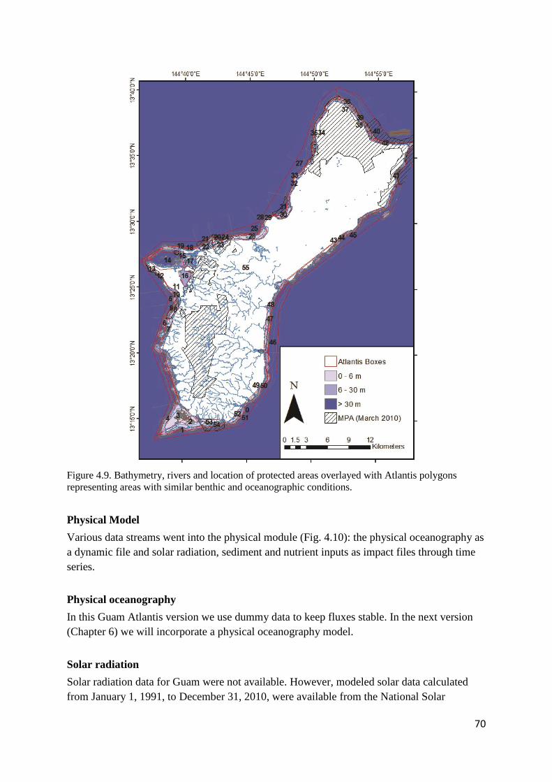
70
Figure 4.9. Bathymetry, rivers and location of protected areas overlayed with Atlantis polygons
representing areas with similar benthic and oceanographic conditions.
Physical Model
Various data streams went into the physical module (Fig. 4.10): the physical oceanography as
a dynamic file and solar radiation, sediment and nutrient inputs as impact files through time
series.
Physical oceanography
In this Guam Atlantis version we use dummy data to keep fluxes stable. In the next version
(Chapter 6) we will incorporate a physical oceanography model.
Solar radiation
Solar radiation data for Guam were not available. However, modeled solar data calculated
from January 1, 1991, to December 31, 2010, were available from the National Solar

71
Radiation Database.5 Photosynthetically Available Radiation (PAR in Einstein/m
2/day) was
available for Guam from satellite data and obtained from NOAA’s Coast Watch for 2002–
2010.6 This dataset was corrected for the influence of islands and the average for an eight-day
interval was computed. We then converted the values to solar data in W/m2 to compare it
with the modeled data output. As the seasonality was similar between the two datasets and
because the modeled time series comprised a much longer time span we used those data for
the Atlantis model (Fig. 4.11).
Figure 4.10. Schematic overview of the Atlantis framework and requirements for the physical
oceanography module and resulting force.prm file.
Figure 4.11. Solar radiation data calculated from satellite derived photosynthetically active radiation
data (red line: NOAA’s Coast Watch)7 and modeled data (blue line: National Solar Radiation
Database)8.
5 rredc.nrel.gov/solar/old_data/nsrdb/
6 coastwatch.pfeg.noaa.gov/erddap/griddap/erdMHpar01day.html
7 coastwatch.pfeg.noaa.gov/erddap/griddap/erdMHpar01day.html
8 rredc.nrel.gov/solar/old_data/nsrdb/
0
2000
4000
6000
8000
10000
7/4/2002 7/4/2003 7/4/2004 7/4/2005 7/4/2006 7/4/2007 7/4/2008 7/4/2009
Solar (Wh/m2)
METSTAT Glo (Wh/m2)
R-script
Force.prm

72
Salinity and temperature
Salinity and temperature time series were populated with an average value from 9 to 19
conductivity-temperature-depth casts per depth range (surface, 10, 20, 30 m) of surveys
conducted in the dry (April and May) and wet (October) season around Guam. These values
will be updated by the salinity and temperature values from a oceanography model (Chapter
6).
Sediment and nutrient input—forcing files
A flow discharge model has been developed for two watersheds in central Guam, one that
discharges in the Apra Inner Harbor on the west coast and one that discharges in Pago Bay on
the east coast (Tetra Tech 2012). Time series of daily flow discharge rates are available from
five rivers (La Sa Fua, Ugum, Umatac, Inarajan, and Ylig) all in the southern part of Guam
and suspended sediment discharge time series from the La Sa Fua, Ugum, and Ylig River.9
We used these data to estimate sediment input per Atlantis polygon (Table 4.2).
A direct relation between flow rate and nutrient input is not available for Guam.
Therefore, we reconstructed the nutrient input from a watershed with 4 rivers discharging into
Hanalei Bay on the north coast of Kauai, Hawai’i (Table 4.3, data from Tetra Tech). This
watershed shares many characteristics with Guam on their volcanic origin, steep slopes,
vegetation cover, human population size and feral ungulate population. Although far from
ideal, this data set was the closest data set we could find to represent point-source pollution in
bays. Moreover, both flow rates on Guam as from Hanalai Bay were estimated using the
same methods (Tetra Tech 2012). When comparing the slope and intercept of the relationship
of flow rate and sediment discharge from the Hanalei Bay watersheds with the three
watersheds with sediment data from Guam (Table 4.2), it is noticeable that the slope was
orders of magnitude higher for Guam watersheds indicating a much higher sediment
discharge rate compared to Hanalei Bay. This high sediment load can also been seen when
comparing the mean sediment discharge of the watersheds on the two islands. These high
sediment discharge rates are in correspondence with sediment studies conducted on Guam
which concluded that sediment rates in Guam are higher than any other reported values
elsewhere (Wolanski et al. 2003a, Minton et al. 2006, Storlazzi et al. 2009b). To calculate the
sediment discharge from the three rivers where we had flow rates for, I used the mean slope
and intercept of the flow rate and sediment discharge relationship from the Ugum, La Sa Fua
and Ylig River (in red in Table 4.2) and calculated the daily sediment discharge rate based on
the flow rate of those rivers.
9 waterdata.usgs.gov/nwis

73
Table 4.2. Characteristics of four rivers in the Hanalei Bay watershed, Island of Kauai, and seven
rivers in central Guam and the slope and intercept of the linear relationship between flow rate (in m3
per second) and sediment discharge rate (in grams per second). Calculated values for Guam in red.
Island River
Watershed
area km2
Atlantis
Polygon
ID
Mean
flow
rate
m/s
Mean
sediment
discharge
g/s Slope intercept R2
Data period
mm/yy–
mm/yy
Kauai Hanalei 0.89 NA 7.65 0.18 0.1376 1.6279 0.86 06/00–06/06
Kauai Waioli 0.81 NA 1.58 0.23 0.0073 -0.1893 0.71 06/00–06/06
Kauai Waipa 0.17 NA 0.67 0.05 0.0074 -0.1144 0.80 06/00–06/06
Kauai Waikoko 0.060 NA 0.17 1.63 0.5095 -1.4283 0.95 06/00–06/06
Guam Atantano 0.11 16 0.41 1.4934 -10.519 01/91–01/12
Guam Ugum 5.92 7 0.71 219 1.5446 -17.309 0.71 08/80–07/81;
08/06–08/11
Guam La Sa Fua 1.03 7 0.13 44 1.5937 -1.7681 0.64 10/06–10/11
Guam Umatac 2.08 7 0.24 1.4934 -10.519 10/52–12/76;
10/01–10/11
Guam Pago 8.42 48 0.83 1.4934 -10.519 01/91–01/12
Guam Ylig 6.53 48 0.76 355 1.342 -12.479 0.64 08/80–10/81
Guam Inarajan 4.34 52 0.50 1.4934 -10.519 10/52–12/82
Table 4.3. Slope, intercept and R2 of the relationship between NOx and flow discharge rate and NH4
and flow discharge rate for four discharge points in the Hanalei Bay. g/s is grams per second, flow
was in cubic square feet. The mean is from Waipa and Waikoko which have similar flow rates as
Guam’s watersheds (Table 4.2).
NOx g/s NH4 g/s
River Slope intercept R2 Slope intercept R
2
Hanalei 0.000009 -0.0013 0.76 0.000004 -0.0006 0.75
Waioli 0.0003 -0.0069 0.93 0.0007 -0.0173 0.94
Waipa 0.0001 -0.0015 0.95 0.0004 -0.0038 0.95
Waikoko 0.0003 -0.0007 0.95 0.0007 -0.0019 0.96
mean 0.0002 -0.0011 0.00055 -0.0029
For all rivers on the east coast of Guam I further assumed a similar flow discharge
rate as from the Pago, Ylig, and Inarajan rivers. For all rivers on the west coast with its
steeper watersheds, I assumed a similar flow discharge rate as from the Umatac, Ugum and
La Sa Fua rivers for the Atlantis polygons south of Apra Harbor and from the Antantano
River in the Apra Inner Harbor and north of Apra Harbor (Table 4.4). Where necessary I
reconstructed time series starting at January 1, 1991, and ending at December 31, 2012, by
repeating the first or last years. Because of the large discrepancy in the sediment load
between Hanalei Bay and the watersheds in Guam, I multiplied the calculated nutrient
concentrations by 257 (the difference in sediment concentration).

74
In the version of the model presented here, sediment and nutrient inputs are modeled
as inputs to coastal model cells adjacent to land with river mouths and sewage pipes. Guam
Atlantis includes half saturation constants for each primary producer for their growth on
dissolved organic nitrogen to account for the difference in productivity and nutrient limitation
effects on the physiology of growth. The effects of sediments on corals are not incorporated
in this version.
Table 4.4. Summary information on the reconstruction of sediment and nutrient input data in Atlantis
polygons along the southern part of Guam.
Atlantis
Polygon
Id
Correction factor
for number of
point sources
discharging into
Atlantis polygon
Sediment
discharge
relationship
with flow rate
River used to
calculate nutrient
and sediment
discharge based on
flow rate
Source empirical
relationship between
nutrients / sediments
and flow rate
Source
flow rate
7, 8, 10 6, 2, 0.5 Ugum, La Sa
Fua, Ylig
Umatac, La Sa Fua,
Ugum
USGS (SED) &
Tetra Tech (NUT)
USGS
16, 17,
22, 23,
24, 26,
30, 32
1, 1,
1, 1,
0.5, 1
1, 0.5
Antantano Antantano USGS (SED) &
Tetra Tech (NUT)
USGS
48, 49 3, 1.5 Ylig Pago, Ylig USGS (SED) &
Tetra Tech (NUT)
USGS
52 1 Ylig Inarajan USGS (SED) &
Tetra Tech (NUT)
USGS
Ecological Model
Figure 4.12. Schematic overview of the Atlantis framework and requirements for the ecological
module with resulting functional groups and biological related parameter files.
Groups.csv
Biology.prm

75
Rationale for Selection of Modeled Functional Groups
A large biological data set was needed for the ecological module (Fig. 4.12). Species and
functional groups were included in the model with the aim of representing community
dynamics of the nearshore reef, including dominant species sampled by NOAA CRED and
Guam monitoring programs. The number of trophic links and functional groups are important
for the robustness of the model with, in general, more links and less groups leading to a
greater recovery after a disturbance (Pinnegar et al. 2005). Additionally, omission of species
or groups can be preferable to inclusion based on tenuous understanding and arguments
(Fulton et al. 2003a, Johnson et al. 2009). Atlantis requires three detritus groups and the
remaining functional groups are defined by the user. Guam Atlantis includes 42 functional
groups: 3 detritus groups, 2 bacteria groups, 5 plankton groups, 3 benthic algal group, 3
sessile and 6 mobile invertebrate groups, and 20 vertebrate groups (Table 4.5). Species were
aggregated into functional groups on the basis of diet, life-history characteristics, habitat
preferences, ecological role in coral reef processes and whether they were targeted in reef
fishery. Overall the functional groups selected are a compromise, intended to capture the
major ecological responses (at the guild level) and responses to fishing, terrestrial inputs and
climate change, at a taxonomic resolution relevant for fisheries and management decisions.
Table 4.5. Categorization of species data. Trophic level and functional group categorization of the
coral reef ecosystem species based on their diet, habitat, life-history characteristics, ecological role,
and interest to fishers and managers.
No Functional groups
Atlantis
Code Species/description
Trophic
level
Fishery
target
sp Importance of inclusion
1 Carrion DC dead detritus
nutrient recycling, part of
microbial food loop
2 Refractory detritus DR long 'life' time detritus
nutrient recycling, part of
microbial food loop
3 Labile detritus DL easily degraded detritus
nutrient recycling, part of
microbial food loop
4 Pelagic Bacteria PB
hetrotrophic bacteria
(0.2-1 um)
bottom
food web
nutrient recycling, part of
microbial food loop,
consume DOM/EOC from
phytoplankton and
macroalgae
5 Benthic bacteria BB
hetrotrophic bacteria
(0.2-1 um)
bottom
food web
nutrient recycling, part of
microbial food loop,
consume DOM/EOC from
phytoplankton and
macroalgae
6 Small phytoplankton PS
picoeukaryotes,
cyanobacteria, < 1um
primary
producer
part of microbial food loop,
release DOM/EOC for
uptake by hetrotrophic
bacteria
7 Large phytoplankton PL incl. diatoms
primary
producer
main food for benthic filter
feeders
8 Turf algae TURF algae < 1cm
primary
producer
nutrient exchange between
sediment and water column,
facilitates coral and CCA
recruitment
9 Macroalgae MA algae > 1cm
primary
producer
space competitor with
corals, decreases coral and
CCA recruitment

76
No Functional groups
Atlantis
Code Species/description
Trophic
level
Fishery
target
sp Importance of inclusion
10
Crustose-coraline
algae CCA
primary
producer
reef builder facilitates coral
recruitment
11
Zooplankton -
herbivores ZH
copepods,
appendingularias
bottom
food web
most abundant herbivore,
part of microbial food loop,
consume hetrotrophic
bacteria and small
phytoplankton, 'sloppy'
predation leads to
remineralization (NH4,
dissolved free amino acids,
etc)
12
Zooplankton -
carnivores ZC
chaetognath,
euphausiids,
amphipods, crab larvae,
isopods, mysids,
polychaetes
bottom
food web
main food for benthic filter
feeders, consume small
zooplantkon (prefer
ciliates), small phytos up to
200 um
13 Demersal zooplankton ZD
pelagic fish & invert
larvae, copepods,
polychaetes,
foraminiferas
bottom
food web
vertical migration,
important food source for
benthic filter feeders
14 Benthic carnivores BC
e.g., polycheates,
swimming crabs, cones,
tritons, burrowing
crustaceans, flatworm,
sea snail, nudibranch,
mantis shrimp
bottom
food web
nutrient recycling, bottom
foodweb, carnivorous diet
15 Benthic detritivores BD
e.g., brittle stars,
detritivorous
polychaetes, peanut
worms, crabs, shrimps,
lobsters
bottom
food web
nutrient recycling, bottom
foodweb, detritivorous diet
16 Benthic meiofauna BM
e.g., squat lobsters,
limpets, top snails,
chitons, snapping
shrimps, hermit crabs,
abalones, cowries
bottom
food web
nutrient recycling, bottom
foodweb, mostly
herbivorous diet
17
Benthic suspension
feeders BFF
octocoral, sponges,
tunicates, zooanthids,
giant clams, bivalves,
polychaetes,
foraminifera, bryzoans,
brittle stars
bottom
food web
suspension feeders -
important source of carbon
uptake
18
Branching (sheltering)
corals CRS
corals that provide
shelter: e.g.,
Pocillopora, Acropora,
branching Porites,
Heliopora, Echinopora.
bottom
food web
frame builders of reef
ecosystem, important
primary producers and
suspension feeders, less
susceptible to disease,
predation, acidicification &
ocean temperature increase
19
Massive/Encrusting
(non-sheltering) corals CRN
corals that provide less
or no shelter: e.g.,
massive Porites,
Leptastrea. Favia,
Astreopora, Montipora,
Goniastrea, Cyphastrea bottom
food web
frame builders of reef
ecosystem, important
primary producers and
suspension feeders,
susceptible to disease,
predation, acidicification &
ocean temperature increase
20 Cephalopods CEP octopus, squids invertebrate x important diet component
21 Benthic Grazers BG
urchins (helmet
collectors, pencil,
boring urchin, diadema) invertebrate x
grazer, keeps algal biomass
low promoting coral cover
and coral recruitment
22 Sea Stars BSS
including crown-of-
thorns seastar invertebrate
coral predator

77
No Functional groups
Atlantis
Code Species/description
Trophic
level
Fishery
target
sp Importance of inclusion
23 Sharks SHR
reef-associated sharks
(gray reef, whitetip reef,
Galapagos, blacktip
reef, tawnry nurse
shark)
apex
predator x
controls lower trophic
groups, fast swimming
roving, long life span
24 Rays RAY stingrays apex predator
important to keep urchins &
sea stars population size in
control
25 Roving piscivores FPR
jacks, snappers,
barracudas
apex
predator x
controls lower trophic
groups, fast swimming,
roving, shorter life span
than sharks
26 Mid-water piscivores FPM
cornetfish, trumpet fish,
houndfish, needlefish apex predator
controls lower trophic
groups, mid-water and
surface water habitat
27 Benthic piscivores FPB
eels, scorpionfish,
lizardfish apex predator
controls lower trophic
groups, benthic habitat
(sedentary)
28
Targer benthic
piscivores TPB groupers
apex
predator x
controls lower trophic
groups, benthic habitat
(sedentary)
29 Bumphead parrotfish BHP
Bolbometopon
muricatum herbivore x
species of special interest,
major agents of bioerosion
on reefs, removing dead
coral and exposing hard,
reef matrix for colonization
by coralline algae and corals
30
Herbivores—
excavators/bioeroders FHE large-bodied parrotfish herbivore x
major agents of bioerosion
on reefs, removing dead
coral and exposing hard,
reef matrix for colonization
by coralline algae and
corals, target species of reef
fishery
31
Herbivores—scrapers FHS small-bodied parrotfish herbivore x
limiting the establishment
and growth of macroalgae
while intensely grazing
epilithic algal turf, and
providing areas of clean
substratum for coral
recruitment;
< 35 cm
32
Herbivores—grazers FHG
schooling;small
angelfishes (all
Centropyge species),
and many species of
surgeonfishes (all
Zebrasoma and
Acanthurus species
except those that feed
exclusively on plankton
or are grazers /
detritivores) herbivore
intensely grazing epilithic
algal turfs, decreasing the
establishment and growth of
macroalgae
33 Target herbivore—
grazers
TGR
rabbitfishes,
surgeonfish herbivore
x intensely grazing epilithic
algal turfs, decreasing the
establishment and growth of
macroalgae

78
No Functional groups
Atlantis
Code Species/description
Trophic
level
Fishery
target
sp Importance of inclusion
34 Herbivores—browsers FHB
batfishes and
parrotfishes of the
genus Calotomus and
Leptoscarus herbivore
selecting individual algal
components and remove
only algae and associated
epiphytic material, thus
reducing coral overgrowth
and shading by macroalgae,
and can play a critical role
in reversing coral-algal
phase shifts
35
Target herbivore—
browser THB
unicornfishes,
rudderfishes, herbivore x
selecting individual algal
components and remove
only algae and associated
epiphytic material, thus
reducing coral overgrowth
and shading by macroalgae,
and can play a critical role
in reversing coral-algal
phase shifts
36 Detritivores
FDE Surgeonfish (mostly
Ctenochaetus sp),
detritivore
important for recycling
nutrients, feed on
decomposing plant and
animals parts
37 Invertivores
FIV triggerfish, hawkfish,
filefish
invertivore
important to keep urchins &
sea stars population size in
control
38 Target invertivore
TIV wrasse, emperor,
snapper, goatfish,
squirrelfish, sweetlips invertivore x
important to keep urchins &
sea stars population size in
control
39 Humphead wrasse
HHW
Napolean wrasse,
Cheilinus undulates invertivore x
species of special interest,
important to keep urchins &
sea stars population size in
control
40 Coralivores
FCO
most butterflyfishes invertivore
coral predator, also coral
disease vector
41 Planktivores
FPL
soldierfish, cardinalfish,
some unicornfish,
fusiliers, chromis planktivore
Feed on plankton and
detritus (algal material),
important in recycling
nutrients and importing
allochtonous carbon,
nitrogen
42 Turtles
REP green turtle, Chelonia
mydas herbivore x
herbivore, crop macroalgae,
keep turf low
Inclusion of Microbial Foodweb
Including the microbial foodweb increases total energy throughput and energy transfer
efficiency (TE) from detritus but decreases the TE from primary productivity; this
phenomenon could be a result of enhanced recycling of materials and energy by microbes and
represent the system behavior better than excluding this foodweb (Paves and Gonzalez 2008).
Various studies have searched for significant sources of nutrients that could explain the high
reef productivity, such as, groundwater discharge in highly porous volcanic islands (Street et
al. 2008) and pelagic bacterial uptake by suspension feeders (Bak et al. 1999). In pelagic
eutrophic regions, large (> 5 µm) phytoplankton is grazed on by zooplankton which is eaten
by planktivorous fish resulting in a short food chain. However, in oligotrophic regions a
longer food chain that includes a microbial loop, dominates. In these systems, pico and nano-
sized auto- and heterotrophic organisms dominate the planktonic biomass and production

79
(Campbell et al. 2003). Corals and other filter feeding benthic organisms capture these small
particles and so introduce nutrients to the food chain (Ribes et al. 2003, Genin et al. 2009).
Phytoplankton makes a small contribution to primary production on an area-specific basis,
but if currents flow over the reef then much of their production may pass into the reef-food
webs (Jennings et al. 2001). This grazing is a principal pathway through which allochtonous
nutrients and suspended particulate matter are imported to a reef community from the flowing
water (Fabricius and Dommisse 2000). The close coupling between primary production and
heterotrophs (respiration) ensures efficient nutrient recycling (Duarte and Cebrian 1996) and
small (< 20% net primary production) allochtonous carbon input can cause shifts to a net
heterotrophic state (Odum and Odum 1955). In coral reefs roughly 50% of the net primary
production produced offshore and on the reefs is channeled through the microbial loop
(Azam et al. 1983, Pernthaler 2005, Zöllner et al. 2009). This high efficiency sustains the fish
and invertebrate populations on the reef. The majority of algal production (20%–90%) is
grazed and much of this leads directly to the production of fished biomass (Polunin and
Roberts 1996).
Inclusion of 19 Functional Groups of Fishes
The trophic structure of tropical fish assemblages encompasses a larger trophic spectrum than
temperate assemblages. In addition to invertivores and piscivores, tropical communities
include various herbivores, sessile and mobile invertivores and zooplanktivores. These
additional trophic groups ensure a better use of low-quality food resources, such as algae,
seagrasses and sessile invertebrates compared to temperate systems (Harmelin-Vivien 2002).
Coral reef fish have also been able to reach a speciation rate that is much higher than in
temperate waters. For example, surgeon fishes of the genus Ctenochaetus are highly derived,
they ingest about 85% of CaCO3 and only exist in the Indo-Pacific; the obligate corallivorous
butterflyfishes are also absent from temperate waters and found mostly in the western Pacific;
parrotfishes have evolved to various genera that ingest a high percentage of CaCO3 in the
Indo-Pacific whereas in the Atlantic these species only browse on algae (Harmelin-Vivien
2002).
For the Atlantis model, coral reef fish were grouped into functional groups based on:
1. Diet: main (> 50%) food item is plants/plankton/inverts/coral/detritus/fish based on
literature, Fishbase (www.fishbase.org) and expert opinion;
2. Feeding habit (ecological role): grazing/browsing/excavating/scraping/hunting/plankton
feeding based on literature, Fishbase and expert opinion;
3. Habitat: within 1 m above substrate, in water column, mid-water and on surface, roving
based on literature and expert opinion;
4. Life history parameters: maximum length, growth rate (k), maximum age (e.g., sharks are
classified separately from other large roving piscivores such as jacks; large bodied and
small bodied parrotfish are separated);
5. Commercial, cultural, ecological or management interest (e.g., humphead wrasse and
bumphead parrotfish are both species of concern).
80
These important specializations were determined based on ecological literature
available for coral reef fish (e.g., Bellwood et al. 2004, Cvitanovic et al. 2007, Friedlander et
al. 2007b, Jennings et al. 2001, Green et al. 2009), discussions with resource managers and
coral reef fish specialists (Brett Taylor, Terry Donaldson, University of Guam; Ed DeMartini,
Ivor Williams, PIFSC) and participants at the November 2012 Guam workshop (Weijerman
and Brown 2013).
Coral reefs in Guam, as elsewhere, exhibit phase shifts from coral to macroalgal
dominance (Mumby 2006, Friedlander et al. 2008). Therefore, we further split up the
herbivore fish group based on their role in preventing this phase shift from happening and in
promoting resilience of the reef in order to better model reef processes (Green et al. 2009).
Surgeonfish and some damselfish species (denuders or grazers) and parrotfish and urchins
(scrapers and excavators) play a crucial role in preventing macroalgae (defined here as all
foliose algal species > 1 cm standing stock) from emerging from algal turf (defined as all
foliose algal species ≤ 1 cm) by their high feeding rate on turf algae (Steneck 1988, Bellwood
et al. 2006) and so prevent coral overgrowth and shading by macroalgae (Bellwood et al.
2004). Yet they can only maintain the reef in a cropped state if coral cover does not decrease
substantially (Williams et al. 2001, Mumby 2006), and they are not very effective in the
reversal of a phase shift (Bellwood et al. 2006). Browsers are species that prefer to feed on
macroalgal stands and could play a crucial role in the reversal of a phase shift. Excavators,
and to a lesser degree scrapers, are those species that have a functional role in bioerosion, by
scraping off (dead) coral and sediment and so facilitate coral and coralline algal recruitment
(Bellwood et al. 2004). These last two groups consist entirely of parrotfishes and the bigger
they are, the larger are their bites so the higher their effectiveness (Bruggemann et al. 1996,
Ong and Holland 2010, Comeros-Raynal et al. 2012).
The world’s largest parrotfish, the bumphead parrotfish, Bolbometopon muricatum, is
an important bioeroder on a reef and a coral predator. They bite the substratum, shaping the
corals and the coral reefs and remove up to five metric tons of calcium carbonate (half of
which is live coral) annually (Bellwood and Choat 2011). Hence, their ecological role as
bioeroders and facilitators of coral recruitment by preventing algal overgrowth is very
important to the well-being of a reef (Bellwood and Choat 2011). However, because they can
grow so large, sleep in groups in shallow water and spawn in large aggregations they are
easily targeted by fishers and vulnerable to extinction (Comeros-Raynal et al. 2012). Visual
sightings of the B. muricatum in Guam are nowadays rare and they could be locally extinct
(Bellwood et al. 2003, Fenner 2012). Just like the bumphead parrotfish, the humphead
wrasse, Cheilinus undulates, is also an iconic species and shares many of its life-history
characteristics with the bumphead parrotfish (Donaldson and Dulvy 2004). Both species are
listed as threatened on the IUCN red list and as a species of concern (SOC) to NOAA
Fisheries. As iconic reef inhabitants, they could be a very important component to the dive
industry making them not only ecologically important but also economically (see Chapter 8).
Because of these important role, we included B. muricatum and C. undulates in the model as
their own functional groups.
Our species assignments to the 19 functional groups (Table 4.5) were further checked
based on various published sources (Bellwood and Choat 1990, Choat and Robertson 2002,

81
Friedlander and DeMartini 2002, Green et al. 2009, Sandin and Williams 2010), FishBase10
and expert opinion.
Seabirds and Marine Mammals
We did not include any seabirds or marine mammals in Guam Atlantis as we assume that
their contribution in terms of production or extraction to the coral reef ecosystem is small as
they either forage on the intertidal habitats or offshore on small pelagics. The same holds true
for the resident dolphins that rest in some of Guam’s shallow bays but feed offshore.
4.3.2 Data Sources
Data sources for the biological parameters and biomass and abundance data came
predominantly from monitoring studies conducted by NOAA PIFSC CRED in 2011. These
data were supplemented with data from Guam DAWR, Coastal Management Program and
University of Guam marine Laboratory monitoring programs, peer-reviewed literature,
technical reports, theses and expert opinion. Fish and benthic survey methods used by CRED
are detailed in Richards et al. (2011), Brainard et al. (2012) and Williams et al. (2012) and are
only briefly described here. Extensive fish and benthic surveys conducted by CRED in 2011
(Fig. 4.13) used a stratified random sampling design and incorporated shallow (0–6 m), mid-
depth (6–18 m) and deep (18–30 m) sites (Williams et al. 2012). Fish surveys were conducted
using a stationary point-count method (SPC) and the benthos was surveyed by analyzing
images from photo-transects along the diameter of the 15 m cylinder. For Guam Atlantis we
combined the results of the two deeper sites for our deep (6–30 m) polygons. Towed-diver
surveys were conducted following a mid-depth (approximately 12–15 m) contour. Data from
the towed-diver surveys were used for biomass estimates of apex predators as these data
represent their biomass better than data from SPC surveys conducted at stratified random
sites (Richards et al. 2011) and for the clustered distribution of seastars. Towed-diver and
rapid ecological assessment (REA) survey data from previous years supplemented data in
Atlantis polygons not covered by 2011 surveys.
Horizontal distribution of species among the Atlantis polygons came from the 2011
data supplemented with expert opinion (e.g., for green turtles and urchins). For apex predator
and roaming species (e.g., jacks, sharks, rays) we assumed an even distribution as these large,
faster swimming species will move more compared to the smaller-sized reef fishes. However,
we adjusted those values by decreasing the numbers in the shallow polygons and scaling
them based on the results from visual surveys. For instance, sharks were predominantly seen
in polygons, 31, 47 and 51 so we increased the percentage for those polygons while
decreasing it for others. Vertical distribution in the water column and habitat preference came
from expert opinion (D. Burdick, Guam Coastal Management Program; V. Brown, NOAA
Pacific Islands Regional Office, Guam; T. Donaldson, University of Guam; I. Williams,
CRED) and literature on habitat affinity (Beukers and Jones 1998, DeMartini and Anderson
2007, Friedlander et al. 2007a, DeMartini et al. 2010, Eriksson et al. 2012, Gratwicke and
Speight 2005, Johansson et al. 2012).
10
www.fishbase.org

82
Figure 4.13. Survey sites around Guam. NOAA’s Coral Reef Ecosystem Division conducts bi-
triennial surveys around Guam. The black dots represent the 133 biological survey sites visited in
2011 whereas the red dots represent the survey sites visited in 2005, 2007, and 2009. The blue slugs
indicate the trajectory of towed-diver surveys from 2005 to 2011.
Parameters for the dynamic files (e.g., growth rate, clearance rate; see section
‘Biomass dynamics’) for invertebrates came from an Ecopath coral reef ecosystem model
developed for Hawai’i (Weijerman et al. 2013; Chapter 3) (Table 4.6) and for vertebrates
they are calculated as outlined in section “Biomass dynamics”.

83
Table 4.6. Invertebrate functional groups and basic life history parameterization. Growth, clearance,
and mortality rates are postcalibration values. Initial life history parameters were based on Chapter 3.
Code Group
Maximum
growth rate
(mgN/day)
Clearance
(mg3/mgN/day)
Linear
mortality
(/day)
Quadratic
mortality
(/day)
CEP Cephalopods 0.022 0.002
BSS Sea Stars 0.013 0.001 0.00001 0.00001
BG Sea Urchins 0.014 0.001 0.0001 0.005
CRS Branching Corals 0.006 0.006
CRN Massive Corals 0.003 0.003
BFF Benthic Suspension Feeders 0.007 0.001
BD Benthic Deposit Feeders
(Meiofauna)
0.033 0.003
BC Benthic Carnivores 0.023 0.002
BM Benthic Meiofauna 0.022 0.002
ZD Demersal Zooplankton 0.366 0.037 0.000001
ZC Carnivorous Zooplankton 0.323 0.032 0.000001
ZH Herbivorous Zooplankton 0.409 0.041 0.000001
Life history parameters (mortality, growth constant (k), infinite length (Linf), age at
first maturity, pelagic larval duration, maximum age) for fish and sharks were obtained from
literature (MacDonald 1981, Victor 1986, Wellington and Victor 1989, Sudekum et al. 1991,
Choat and Axe 1996, Hart and Russ 1996, Wilson and McCormick 1999, Choat and
Robertson 2002, Gust et al. 2002, Sadovy et al. 2003, Choat et al. 2006, Hamilton et al. 2008,
Longenecker and Langston 2008, Schluessel 2008, McIlwain et al. 2009, Ishihara and
Tachihara 2011, Rhodes et al. 2011, Taylor et al. 2012), empirical formulas, FishBase and
expert opinion (Brett Taylor, Terry Donaldson, University of Guam; Ed DeMartini, Marc
Nadon, PIFSC). In absence of data on natural mortality (M) I used an empirical relationship
(Pauly, 1980):
log(M) = -0.066-0.279*LOG(Linf)+0.654*LOG(k)+0.463*LOG(T) Eq. 1
where Linf is asymptotic total length in cm, k is the growth constant from the Von Bertalanffy
equation (both from literature or FishBase), and T is the mean temperature on the reef in °C
and was obtained from CRED in situ data.
If, based on the calculated M, the chance that a species would reach its maximum age
was less than 0.01%, we recalculated the maximum age (tmax) based on the mortality-
longevity assumption:
tmax = ln(0.01)/-M Eq. 2
We then checked the chance that the functional group would reach its (weighted
mean) maximum age and if this chance was < 0.01% we used the natural mortality based on
the mortality-longevity assumption. For all the functional groups targeted in the reef fishery
we used tmax to calculate M as fishing affects Linf used in Equation 1 (Table 4.7).

84
Table 4.7. Natural mortality estimates used in the model (see text for calculation).
Functional Group M in Years Functional Group M in Years
Sharks 0.21 Target herbivore—grazers 0.19
Rays 0.17 Herbivores—browsers 1.06
Roving piscivores 0.16 Target herbivore—browser 0.32
Mid-water piscivores 0.51 Detritivores 0.26
Benthic piscivores 0.53 Invertivores 0.61
Targer benthic piscivores 0.29 Target invertivore 0.49
Bumphead parrotfish 0.14 Humphead wrasse 0.15
Herbivores—
excavators/bioeroders 0.41 Coralivores 1.05
Herbivores—scrapers 0.53 Planktivores 1.24
Herbivores—grazers 0.70 Turtles 0.07
Life history information for sea turtles came from literature: the von Bertalanffy
growth constant k = 0.089 yr–1
(SD 0.015) and Linf = 108.9 cm were based on Caribbean
green sea turtles (Frazer and Ehrhart 1985); length-weight parameters were based on green
turtles from Hawai’i (Balazs and Chaloupka 2004), age at sexual maturity was estimated at
18–27 y for a 99 cm carapace length with a comment that the upper estimate is more realistic
(Frazer and Ehrhart 1985) and between 35 and 40 y for main Hawaiian Islands and > 50 y for
Midway Atoll in the Northwestern Hawaiian Islands (Balazs and Chaloupka 2004). We used
37.5 y for the Guam Atlantis model. Juvenile green turtles leave their pelagic habitats at a
carapace length of 35 cm (5 kg) when they are approximately 6 years old.
Appendix A includes all fish species per functional group with their scientific and
common names, family, trophic level, the CRED method used for biomass estimate, biomass
estimate and the average annual catch (DAWR, WPacFIN). Appendix B includes life history
data as a weighted mean value per functional group.
Primary producers and invertebrates are modeled as biomass pools per area (mgN/m2)
for benthic organisms and per volume (mgN/m3) for pelagic organisms. Vertebrate groups are
divided into 10 age classes each tracked by the abundance and weight at age to allow for
ontogentic shifts. Weights are measured through structural (bones and other hard parts) and
reserve (muscles, fat, reproductive organs, and other soft tissue) weight (mgN/m2).
Most available biological data were reported in grams wet weight per area or per
volume. As the currency of Atlantis is nitrogen we converted wet weight to nitrogen by
dividing it by 5.7 (based on the Redfield ratio) and by assuming dry weight equals to 5% of
wet weight. We used a mean depth of 15 m to convert area specific data to volume specific
data where needed. Weijerman et al. (2014a) gives general information about each functional
group, their diet and biomass with data sources.

85
4.3.3 Model Dynamics
Biological Dynamics
Primary Production
Guam Atlantis includes the primary producer groups: macroalgae, turf algae, crustose
coralline algae,and large and small phytoplankton. In a later version of the model (Chapter 6),
code will be adapted for corals to make them both filter feeders (as such included in the
present model) and primary producers. Growth is driven by Michaelis-Menten dynamics and
varies with nutrients, light and space availability. Biomass is lost to predation, lysis, linear
and quadratic mortality and harvesting. The rate of change in biomass B for a primary
producer group is:
dB/dt = G - Mlys – Mlin – Mquad - ∑ 𝑀𝑗𝑛𝑗=1 – F Eq. 3
in which G is the growth rate of autotrophs, M is loss as a result of lysis (Mlys), linear
mortality (Mlin) or quadratic mortality (Mquad), Mj is predation mortality as a result of grazer j,
n is number of grazers, and F is mortality from harvesting. The rate of growth is defined as:
G = µ * δirr * δN * δspace * A Eq. 4
where µ is maximum growth rate, δirr is light limitation factor, δN is nutrient limitation factor,
δspace is space limitation factor, and A is rate of catabolism. For formulation of the limitation
factors, see Fulton et al. (2004a), as it varies between producers.
Growth rates were obtained from Chapter 3 and assumed to be similar between
Hawai’i and Guam. During tuning of the model these initial growth rates were adapted (Table
4.8).
Table 4.8. Growth rates for primary producers with alterations made during tuning in parentheses.
Initial growth rate calculated from Chapter 3.
Functional Group Name Growth Rate
Large phytoplankton 0.410 (1.0)
Small phytoplankton 0.410
Macroalgae 0.018
CCA 0.010
Turf algae 0.030
Nutrient Dynamics
Nitrogen is the currency of Guam Atlantis and changes in ammonia (NH) and nitrate/nitrite
(NO) are modeled. Nutrient concentrations effect the growth of primary producers and are
governed by uptake by autotrophs, excretion by consumers, nitrification and denitrification:
d(NH)/dt = -∑ 𝐴𝑁𝐻,𝑖𝑃𝑖=1 + ∑ 𝐸𝑁𝐻,𝑗
𝐶𝑗=1 – S + R Eq. 5
d(NO)/dt = - ∑ 𝐴𝑁𝑂,𝑗𝑃𝑖=1 +S Eq. 6
where A is rate of uptake of NH or NO from the water column by autotroph i, P is set of all
autotrophs, E is excretion of NH by consumer j, C is set of all consumers, S is amount of NH

86
converted to NO by bacteria (nitrification) and R is amount of NH produced by
denitrification.
Biomass Dynamics
Changes in biomass for vertebrate and invertebrate consumers are influenced by growth,
predation, mortality, migration and harvesting:
dB/dt = G – ∑ 𝑀𝑖𝑛𝑖=1 – M + I – E – F Eq. 7
where biomass (B) is substituted for abundance per age-class for the vertebrates, G is growth,
Mi is predation by predator i, n is the number of predators, M is mortality not captured by
predator-prey dynamics, I is immigration into the model which is set to zero for Guam
Atlantis, E is emigration out of the model which is also set to zero for Guam and F is fishing
mortality.
Growth dependents on predation, assimilation efficiency and oxygen and space
availability:
G = ∑ 𝑃𝑖𝑛𝑖=1 * εi * δO2* δspace Eq. 8
where Pi is predation by consumer on prey i, εi is the assimilation efficiency on prey i, and δO2
and δspace are the oxygen and space limitation factors. Oxygen and space limitation apply to
benthic invertebrates living on or in the sediment layer and is governed by a Michaelis-
Menten relationship: oxygen limitation increases with depth and growth is inhibited by
increases in the density of an invertebrate group until a threshold is passed where the
maximum density is reached. Half saturation constants, depth of oxygen horizon, lower
density thresholds, maximum densities and half saturation constant for space limitation were
all adapted from Fulton et al. (2004c). For vertebrates growth is allocated further into
structural and reserve nitrogen pools (Fulton et al. 2004b).
Mortality not captured by the predator-prey dynamics is composed of linear mortality,
quadratic mortality and species-specific mortality (e.g., fouling by epiphytes on macroalgae,
starvation) for each functional group.
Spawning and recruitment also affect biomass dynamics of vertebrates and these
processes are described below.
Predation
In the Atlantis framework, predation can be modeled using various formulas. Fulton et al.
(2003b) concluded that the Holling Type II functional response may predict ecosystem
responses equally well as more complex models, therefore, for Guam Atlantis we
implemented a modified version of the Holling Type II response to model predation:
Pij = 𝐵𝑖∗𝑎𝑖𝑗∗𝐵𝑗∗𝐶𝑗
1+𝐶𝑗
𝑔𝑗(∑ 𝐵𝑖
𝑛𝑖=1 ∗𝑎𝑖,𝑗∗𝐸𝑖𝑗)
Eq. 9
where Pij is ingestion of prey i by predator j (mgN), Bi is biomass of prey i (mgN/m3), aij is
availability of prey i to predator j (unitless), Bj is biomass of predator j (mgN/m3), Cj is the

87
clearance rate of predator j (m3/mgN/d), gj is the growth rate of predator j (/d) and Eij is the
growth efficiency of predator j eating prey i (unitless).
The maximum ingestion rate (Gmax) is the asymptote of this function when prey is
abundant. Multiplying this maximum ingestion rate by an assimilation efficiency over all
food types:
g = Gmax * ε Eq. 10
gives us the maximum growth rate (g) in mgN/d/individual. We assume that the assimilation
efficiency (ε) is 10% for vertebrates and 50% for invertebrates. Ingestion rates for
invertebrates came from Chapter 3 and were multiplied by 1.2 to reflect the maximum
consumption rate which is used in Atlantis.
For fish group, the maximum consumption rate depends on the weight of the predator:
Gmax = CA * WCB
Eq. 11
with the constants CA and CB set to 0.3 and 0.7 respectively and units m3/mgN/d (Hanson et
al., 1997). We used weight estimates from Von Bertalanffy curves (structural and reserve
nitrogen) to obtain maximum consumption for an average individual per age class.
Clearance is a measure of feeding efficiency when prey is scarce, i.e., at the origin of
the predator-prey functional response. It reflects the rate at which growth increases with
increased food abundance. Atlantis considers clearance as filter feeding a volume of water or
swept-volume predation with units m3/mgN/d. We assumed clearance rates to be 10% of the
maximum growth rates.
The availability parameter (a) is a combined measure of prey preference and the
relative availability of the prey to the predator. To derive these parameters we constructed a
diet matrix to define the relative contribution of each prey group to each predator’s diet, and
set the a parameters equal to represent these binary predator/prey links and to qualitatively
capture the strength of these links. During model tuning we calibrated these values,
attempting to match realized diets (predicted by Atlantis) to observed diet fractions from field
studies and to match realized growth (size-at-age) to expected size-at-age.
The amount a predator eats not only depends on the availability of its prey but also on
the gape size for age structured predator/prey relationships (Karpouzi and Stergiou 2003). In
general I assumed that a predatory fish can eat a prey fish of 40% of its body length. I used
the weighted means of the morphometric data per functional group to calculate the upper
limits of gape size as the largest prey body length to the maximum predator body length ratio.
For example for jacks that eat fish, molluscs, shrimp and other benthic invertebrates, I divide
the maximum length of the largest prey based on its diet composition, in this case
invertivorous fish (25 cm) by the mean length for roving piscivores (the functional group of
jacks; 73.5 cm) and so calculate the upper limit as 0.46 (Table 4.9). For species that take bites
of their prey, size of the prey is not important. Therefore, for the functional group sharks we
set the upper limit to 3.

88
Table 4.9. Estimation of gape size per Guam Atlantis functional group that preys upon age-structured
groups.
Predator Functional
Group
Dominant Prey
Functional
Group
Weighted Max
Length Predator
(cm)
Weighted Max
Length Prey
(cm)
Upper
Gape
Limit
Mid-water piscivores Planktivores 70 21 0.30
Roving piscivores All fish species 153 70 0.46
Target Benthic
piscivores
Invertivores 50 25 0.50
Benthic Piscivores Invertivores 67 25 0.37
For planktivorous, corallivorous, detritivorous and herbivorous fish, turtles and
invertebrates which do not eat age-structured prey, I defaulted to 0.2 for the upper gape limit.
For invertivorous fish and rays I used 0.25. All functional groups had 0.0001 as the lower
gape limit.
Assimilation
Gross growth efficiency (GGE) is the ratio of production to consumption and for most groups
has values between 10% and 30% (Christensen and Pauly 1992). Exceptions are top
predators, such as marine mammals and seabirds, which can have lower GGE (between 0.1%
and 1.0%), and small, fast-growing fish larvae, nauplii and bacteria, which can have higher
GGE (between 25% and 50%). For example, copepods, the most abundant pelagic grazers,
have a fairly high efficiency to assimilate carbon: the mean GGE is 25% but can exceed to
60% in places with high food concentrations (Hassett and Boehlert 1999); pelagic bacteria
have a GCE of 40% (Cole et al. 1988) but larger invertebrates, such as sedentary octopus, can
also have high GGE of 40%–60% (Jennings et al. 2001). I constrained the assimilation
efficiency to be 80% for most carnivorous groups, i.e., ~ 80% of the consumption is assumed
to be physiologically useful for consumer groups while the nonassimilated food (20%,
consisting of urine and feces) is directed to detritus. Of this 80%, the majority of energy is
used in respiration and a small fraction (e.g., one-eighth) might be translated into growth of
the individual (e.g., an overall 10% GGE). However, for herbivores and detritivores this
default value of 80% often underestimates egestion. I have, therefore, adjusted assimilation
efficiency for detritivorous and herbivorous fish groups to 20%–35%, for demersal and
carnivorous zooplankton to 30%–45%, for herbivorous zooplankton to 50%–55% and for in-
and epifauna to 30%–50% (Edward 1986, Jobling 1994, Cury and Christensen 2005).
Spawning and Recruitment
The alpha and beta parameters in the Beverton-Holt stock recruitment relationship (Beverton
and Holt 1957, 1993) are related, respectively, to unfished level of recruitment and
productivity of the stock at low stock sizes (Equation 12). The steepness of this relationship is
defined as the fraction of recruitment from an unfished population obtained when the
spawning biomass is 20% of its unfished level (Mace et al. 1988). However, setting these

89
parameters is a challenge (Mangel et al. 2010). For stocks where environmental drivers rather
than the parental stocks are important to recruitment the steepness is often set to 1 and for
stocks where the number of recruits are dependent on the parental stock the steepness
approaches 0.2; in general the steepness depends on the demography of the stock (Mangel et
al. 2010). For an age-structured population without fishing the steepness depends on the
schedule of survival and fecundity at age and maximum per capita productivity.
From meta-analyses of stock-recruitment data for several pelagic species, a family-
level median steepness has been estimated that varied between 0.28 for Anoplopomatidae
(Anplopoma fimbria) and 0.95 for Lujanidae (Lutjanus campechanus) (Myers et al. 1999).
For the Guam Atlantis model steepness estimates were used for reef-fish families from Myers
et al. (1999) and interpolated for other families based on their dependence on parental stock
for recruitment.
In Atlantis I used the Beverton-Holt stock recruitment model defined as:
recruits = α*S / (β + S) Eq. 12
where recruits is the number of recruits in the whole system and a recruit is typically a ~ 30–
90 day old post-settlement fish, S is the spawning biomass of mature adults of both sexes in
mgN, α is the maximum number of recruits that can be produced, and β is the level of S that
produces one half of the maximum number of recruits.
The alpha and beta parameters for spawning fish species are critical for tuning the
model and were changed in adjusting model dynamics (Table 4.10). To calculate these
parameters, we made the following assumptions:
stocks have an equal birthrate of females and males;
species or families where genetic results show that they are predominantly self-
seeding, have a great dependency on the parental stock and, therefore, a low
steepness;
the biomass in the MPAs multiplied by an adjustment factor of 1.5 (total fish biomass
around unfished northern Mariana islands is approximately 1.5 times higher than from
MPAs in Guam) is equal to the unfished biomass in Guam (Williams et al. 2012).

90
Table 4.10. Beverton and Holt alpha and beta recruitment parameters for fish groups. Only when
values changed during tuning are they given in the post-tuning columns.
Functional Group Calculated values Post-tuning values
alpha beta alpha beta
Planktivores 2.28E+06 2.45E+08 2.28E+07
Coralivores 2.10E+05 6.74E+07 2.10E+07
Invertivores 4.50E+05 4.72E+08 4.50E+06
Target invertivores 1.88E+05 8.22E+08 4.00E+06
Humphead wrasse 1.13E+01 2.30E+09 1.13E+03
Detritivores 9.99E+04 5.42E+08 5.00E+06
Browsers 1.18E+04 8.33E+06 2.00E+05
Target browsers 1.97E+04 2.67E+08 1.00E+06
Grazers 6.31E+05 2.29E+08 5.31E+07
Target grazers 1.67E+05 5.89E+08 4.67E+06
Scrapers 9.09E+05 1.53E+09 1.80E+07
Excavators 8.51E+03 1.48E+09 9.01E+05
Bumphead parrotfish 1.97E+01 1.16E+09 4.00E+03
Mid-water piscivores 9.01E+03 4.51E+06 1.35E+05
Roving piscivores 9.66E+03 1.68E+09 1.66E+04 1.68E+07
Target benthic piscivores 6.27E+04 2.20E+07 3.03E+05
Benthic piscivores 9.40E+03 6.76E+07 5.40E+04
Rays Fixed recruit = 1 1.5
Sharks Fixed recruit = 1.5 1.0
Turtles Fixed recruit = 0.5
The functional groups sharks and rays have live young and sea turtles lay eggs, so
their recruitment is modeled using a fixed number of offspring produced per adult. For sea
turtles, recruit per adult is the product of hatch success, nests per year and clutch size; for
sharks and rays, it is a product of number of off spring per female, pregnancy rate, proportion
of females in a population and pregnancy interval. Female turtles lay approximately 120 eggs
per nest with a hatching percentage of 77% (Schouten et al. 1997). They can lay up to 5
clutches per nesting season and females return to their nesting beaches approximately once
every 4 years (Limpus and Nicholls 1988). Nesting season is from April to July with
hatchlings emerging between June and September (Valerie Brown, Dave Burdick pers.
comm.). Mortality rate of hatchlings on the beach and in the shallow coastal area is very high
with estimates of 75% (Burgess et al. 2006). Although the juvenile pelagic stage is about 6
years, I used recruit age of 1 year and truncated the smallest age classes that have high levels
of mortality and diets different from the larger individuals found around Guam. I assumed a
fixed recruitment of 0.5. Growth rate is high for juveniles and declines to negligible when
they reach sexual maturity (Limpus and Chaloupka 1997).
Rays have 2–4 pups and sharks 1–6 and I assumed that both have a pregnancy interval
of 2 years (Braccini et al. 2006, Schluessel et al. 2010). These parameters translate to a

91
maximum production of offspring of 1 and 1.5 per adult for respectively rays and sharks
assuming an equal sex distribution.
4.3.4 Fisheries Module
Figure 4.14. Schematic overview of the Atlantis framework and requirements for the fisheries module
with resulting files including a fishery fleet file, catch time serie, and a harvest file.
A good understanding of the fishery is necessary to be able to simplify it in a model
(Fig. 4.14). The fishing community in Guam includes individuals from a diverse set of
cultures, such as indigenous Chamorro as well as introduced Anglo-American and
Micronesian fishers (Allen and Bartram 2008). The island’s indigenous Chamorro people
were highly skilled fishermen and archeological evidence suggests both reef and pelagic fish
were caught using hooks, spears and nets (Amesbury and Hunter-Anderson 2003). Fishing on
Guam is best considered a subsistence fishery, as commercial fisheries have had negligible
effects on Guam’s economy. Commercial fishers target primarily pelagic species beyond the
0–30-m reef boundaries, while most local fishers target both reef and a few pelagic species.
Both traditional and modern fishing techniques are currently in use on Guam (Hensley and
Sherwood 1993). Common fishing methods include hook-and-line, spearfishing (both snorkel
and scuba), gill nets, drag nets, and cast (or throw) nets; with hook-and-line being the most
commonly used method (DAWR and WPacFIN 1985–2012 fisheries data); the highest
catches were obtained from gill nets, hook-and-line and snorkel spearfishing and the highest
catch-per-unit-effort obtained with surround nets and drag nets (Table 4.11). Each method
requires a varying degree of skill, and allows for different levels of species selectivity.
Fisheries.csv
Harvest.prm

92
Table 4.11. Relative effort based on annual mean number of hours that a gear type was used for shore-
based fishery and the obtained catch and corresponding catch-per-unit-effort (CPUE) per gear type. Data source: DAWR and WPacFIN creel inshore fisheries survey data 1985–2012. gh = gear-hour.
Fishing method
Relative
effort (%)
Relative catch
(%)
Mean CPUE
in kg/gh
Cast Net 7.1 9.1 0.39
Drag Net 0.4 3.3 2.64
Gill Net 13.7 29.2 0.65
Hook and Line 64.0 21.9 0.10
Hooks and Gaffs 2.3 3.0 0.39
Other Methods 4.4 5.3 0.37
Scuba Spear 0.4 1.8 1.55
Snorkel Spear 7.5 24.0 0.98
Surround Net 0.2 2.4 3.12
Fishing in Guam is also of cultural significance, as it is tightly woven with the identity
of the islands’ residents and the tradition of sharing catch with friends and family is a
continuation of the Chamorro culture (Allen and Bartram 2008). In a survey conducted on
fishers participating in pelagic fishing, almost all of the respondents reported ‘regularly
giving fish to family, friends or both’ (Rubinstein 2001). DAWR survey results showed that
only 1 fisher sold the fish at one time, indicating the subsistence or recreational goal of
inshore fishing activities. Fishing also contributes to food security, with households reporting
that 24% of fish consumed was caught by an immediate family member and an additional
14% of fish consumed was caught by a friend or extended family member (Van Beukering et
al. 2007). Fish is an especially important source of food for large cultural events such
baptisms, weddings and village fiestas (Rubinstein 2001).
Chapter 5 explains how we used catch-per-unit-effort data to reconstruct historic fish
biomass trends used for model testing.

93
4.3.5 Socio-economic Module and Visualization of Atlantis Model Output
Figure 4.15. Schematic overview of (top) the Atlantis framework and requirements for the socio-
economic module and (bottom) how to visualize model output.
We have not yet included the socioeconomic module into Guam Atlantis but the
visualization tools in Figure 4.15 are also suitable for the ecology and fishery modules.
4.3.6 Model Tuning and Diagnostics
Adjusting input parameters is an iterative process in which current state (i.e., biomass,
abundance, cover) and rate parameters are adjusted to generate realistic system behavior and
fit model predictions qualitatively to observations. This process is made cumbersome by the
slow run-time of Atlantis which also prohibits any automated estimations of model
parameters. I followed the adjustment procedures as used in previous successful applications
of Atlantis (Horne et al. 2010, Link et al. 2010, Ainsworth et al. 2011a). I calibrated the
dynamic behavior of Guam Atlantis in two phases. In the first phase, I initialized the model
with 2011 estimates of biomass and ran the model forward without fishing. Initial conditions
represent approximately 2011, and simulations were projected for 30 years. Goals for this
phase were to keep functional groups from going extinct and achieve weights-at-age
(structural and reserve weight) within 0.5 and 1.5 and ideally between 0.8 and 1.2 times their
initial biomass (Horne et al. 2010). In the absence of fishing, I assumed that the system,
94
beginning from an exploited ecosystem base in 2011, should return to conditions similar to
those in marine preserves around Guam or better (i.e., higher fish biomass values) as some
forms of fishing are still allowed in the preserves. I used mean estimates from underwater
surveys conducted in preserves around Guam in 2011 as calibration targets (CRED data). I
acknowledge that this method is not ideal as species that are already locally rare (e.g.,
bumphead parrotfish) or at very low levels (apex predators) will not be represented
accurately. Therefore, I also compared these estimates with biomass values from the
relatively pristine reefs around the Northern Marianas (Fig. 4.5) and adjusted them when they
differed more than 1.2 times. The benthic community structure did not vary greatly between
inside and outside marine preserves. For these groups and others for which we did not have
unfished biomass estimates, the goal was merely to produce steady biomass through time that
fall within the range of current observations.
For these simulations I did not include large scale trends in climate or environmental
forcing. Extinctions typically point to excessively high predation levels or extremely low
productivity of the stock. The primary parameters involved with resolving these problems
included growth rates (g in eqs. 9 and 10), clearance rate (C in eq. 9), and predation pressure
dictated by the availability parameter (a in eq. 9). Tuning vertebrate weights-at-age involved
adjusting growth rates, recruit weights, and assimilation efficiencies (ε in eq. 11). When
weight-at-age was stable, vertebrate biomass could be adjusted further by manipulating
Beverton and Holt recruitment parameters and the number of recruits for the non-fish
vertebrates, and linear and quadratic mortality.
In the second phase of calibration, I exercised the model with varying degrees of
fishing pressure to evaluate responses of functional groups when perturbed. For these
scenarios, I did not attempt to simulate fleet dynamics, but rather applied constant fishing on
all fished fish groups throughout the duration of the simulation. I expected biomass to
decrease in response to fishing without going extinct at reasonable levels of fishing pressure.
Generally, I expected highly productive stocks, such as, planktivores to be able to withstand
moderate amounts of fishing mortality, and unproductive, long-lived groups like large-bodied
parrotfish (Chlorurus spp.) and groupers to decline under similar fishing rates. As a very
approximate expectation, at fishing levels equal to the natural mortality rate (M), I expected
functional group biomass to decline by 50% compared to a no-fishing scenario (roughly
assuming that the level of fishing mortality that results in the maximum sustainable yield
[FMSY] = M and biomass at maximum sustainable yield [BMSY] = 50% B0, Gulland 1970).
Cases where biomass was too sensitive or too robust to additional fishing pressure usually
pointed to problems with recruitment, and thus adjusting productivity via recruitment was
generally the best solution.

95
4.4 Results
4.4.1 Initial Calibration: No Fishing Scenario
Our goal in this initial tuning phase was to produce steady biomass and, for vertebrates,
stable weight and density in each age class.
Biomass
Approximate values of unfished or lightly fished biomass in MPAs were available for all fish
groups. In the absence of fishing, most fish groups in the simulations reached that biomass
within 5–10 years after being released from environmental perturbation and fishing pressure.
Some of the piscivore groups did not reach the expected unfished biomass level, most notably
the roving piscivores and rays. In general, long-lived species (e.g., bumphead parrotfish and
sharks) took longer to recover as expected from their life-history characteristics. Our goal for
the invertebrate and primary producer groups was to keep them alive and stable through time,
similar to mass balance procedures in Ecopath models (Polovina 1984). This goal was
reached for the majority of these groups but not for benthic meiofauna, macroalgae or corals
which all died after a few years. Most of the groups stabilized after about 20 years except for
demersal zooplankton that continued to increase. As corals are the focus of our model, further
tuning efforts are necessary. We expect that when the model code is updated with coral reef
specific code (Chapter 6), these trends, at least for corals, which will be both predator and
primary producer, will improve.
Weight-at-age for Vertebrate Groups
Results for weight-at-age (reserve weight) for most age classes were relatively stable and
between the 0.5 and 1.5 of the initial weight as desired with some groups (all the herbivores:
grazers, browsers, scrapers, excavators) remaining close to initial values. The exception was
for the youngest juveniles of many groups, for which weight-at-age dropped immediately to
50% of their initial values. For mature age classes dropping to 50% of initial size-at-age (i.e.,
getting very skinny) hampers the reproduction, so it is important for them to keep their
weight. For juveniles this weight loss is less important, especially since growth at later ages
compensated for this, but in future tuning exercises this should be investigated further.
Density-at-age for Vertebrate Groups
Vertebrate densities maintained an age structure that roughly followed an exponential decline
in abundance with age. The piscivores proved most difficult to tune with only the benthic
piscivores and target benthic piscivores showing a final (year 10–30 and year 30 respectively)
age structure with abundance declining smoothly with age.

96
4.4.2 Secondary Calibration: Constant Fishing Pressure
In the second calibration, I applied constant fishing mortalities to evaluate biomass response
to these harvest rates for each functional fish group. I exerted an increasing fishing pressure
on all vertebrate functional these groups except Fish Invertivores, Fish Herbivore Browsers,
Fish Herbivore Grazers and Fish Benthic Piscivores as these groups are not targeted in reef
fisheries. Biomass declined to half the initial biomass when fishing rates where equal to or
exceeded natural mortality rates except for a few groups, such as, Corallivores, Target Fish
Invertivores, Herbivore Excavators and Target Benthic Piscivores. These latter groups all
showed an increase in biomass possibly as a result of a decrease in intra competition and
inter-specific predation pressure. Results show that slow-maturing groups (Sharks, Turtles
and Bumphead parrotfish) could sustain fishing mortality rates substantially higher than their
natural mortality. For the non-harvested fish groups, the biomass stayed similar to the initial
biomass or increased likely as a result of reduced predation pressure.
4.5 Discussion
Human-induced drivers on the natural resources of Guam have intensified and diversified.
Tourism is a main factor contributing to the island’s economy and the number of tourists
visiting Guam and the island’s resident population has increased steadily over the last few
decades. Furthermore, as a result of the military buildup, military personnel and civilians are
scheduled to move to Guam in the next few years. These changes are projected to have a
profound effect on the island’s land cover (e.g., more surfaced roads, housing), land-based
sources of pollution (e.g., increase in sewage, off roading related runoff) and natural
resources (e.g., through recreational fishing, jet skiing, scuba diving). The resulting
competition for space and resources suggests the need for improved quantitative tools to
evaluate competing socioeconomic costs and benefits. There is also growing recognition that
climate and ocean change affects the coral reef ecosystem and should be taken into account in
management strategies. Coral reef ecosystem management has therefore become increasingly
complex. However, with the improvement in computer power and the maturity of ecosystem
models, such as Atlantis, new tools are now available for management scenario analyses.
The objective of this chapter was to detail the design of the model framework and the
parameterization of the spatial and ecological module. Improvements as described below,
especially for coral dynamics and oceanography, are explained in Chapter 6. With these
improvements, the model is used to tests simple management strategies related to fishing
effort, fishing areas and closures, simple ocean acidification scenarios and changes in nutrient
and sediment loading (Chapter 7). These scenario analyses have been investigated with
Atlantis previously. For instance, Kaplan et al. (2012) tested a series of fishing closures and
gear switches using a California Current Atlantis model, and Griffith (2011) and Kaplan et al.
(2010) considered scenarios for ocean acidification. Fulton et al. (2006) and Fulton and Smith
(2004) tested effects of nutrient loading in Atlantis models in Australia. Finally, even with
relatively simple fishing dynamics, results can be linked to economic models, such as, those
of Arita et al. (Arita et al. 2011, Arita et al. 2013) and Kaplan and Leonard (2012).
The development of the Guam Atlantis model has been useful in integrating available
data streams and identifying data gaps. Shallow (0–30 m) benthic mapping data still remains

97
absent for large stretches of Guam. While data on fish and coral and algal cover are available
through monitoring programs, data on other benthic filter feeders, epifauna (invertebrates
living on top of the benthos), infauna (also called cryptic fauna, invertebrates living in the
sediment or associated with benthic groups) and macroinvertebrates are sparse (e.g., just for
one depth range or one bay) or absent. Additionally, in-situ data on chlorophyll-a are sparse.
Both CRED and Guam Environmental Protection Agency (EPA) collect these data but CRED
only as a snapshot in time every 3 years and EPA only for shallow surface waters and mostly
for impacted bays. As chlorophyll-a is a useful proxy for phytoplankton biomass and,
therefore, represents the bottom of the food chain, better estimates are needed. Furthermore,
stock assessments for coral reef fish are rare and life-history parameters for most species are
very sparse. For example, we needed to extrapolate Beverton and Holt recruitment
parameters from a few species to many of the modeled fish groups.
In this chapter, Guam Atlantis does not include code specific to coral reef dynamics.
The inclusion of coral-algal-grazer dynamics, important in shaping the benthic community,
and factors that influence coral recruitment (sediment, CCA cover, excavators) will greatly
enhance simulations of coral reef ecosystem processes. Furthermore, corals play an important
role not only as a food source but also as refuge for juvenile fish and in the current model
version corals died in the first few years; having corals better represented will likely stimulate
fish biomass and the biomass of benthic invertebrates depending on corals.
The physical oceanography is currently simulated with mean values for temperature
and salinity and stable fluxes. Despite the lack of coral specific code and the oceanic model,
the results of the first two calibration phases show that the model can simulate main
dynamics for most functional groups. Calibration results of no fishing or land-based sources
of pollution showed that the biomass of fish groups reached unfished or lightly fished
conditions. Long-lived species with slow reproduction took longer to recover (e.g., sharks,
humphead wrasse, bumphead parrotfish, and rays) than species with a shorter life cycle, such
as, planktivores, coralivores and detritivores. For some groups (e.g., roving piscivores) the
tuning is still not ideal and better parameters are needed for subsequent calibrations.
Calibration results of constant fishing pressure showed that, as can be expected, most groups
decline in biomass once fishing pressure is equal to or exceeds their natural mortality. Further
calibration to evaluate the model’s ability to replicate historical biomass trends under
historical fishing pressure and environmental changes are described in Chapter 6.

98
A fisherman throwing a cast net to catch juvenile fish in Tumon Bay

99
Chapter 5
Coral reef-fish biomass trends based
onshore-based creel surveys in Guam
Weijerman, M, ID Williams, J Gutierrez, S. Grafeld, B Tibbatts, G Davis. In review. Coral
reef-fish biomass trends based on shore-based creel surveys in Guam. Fisheries Bulletin

100
Coral reef fisheries play important roles in the social and economic welfare of
coastal communities and provide vital non-market functions. The complexities
of these multi-species, multi-gear fisheries pose challenges for fisheries
management. The Guam Division of Aquatic and Wildlife Resources has a
detailed creel survey program that attempts to capture the trends in inshore
fishing activities. In this paper we focus on the Guam shore-based coral reef
fishery (1) to evaluate the past and present fishery characteristics in terms of
catch composition and effort per gear type, and (2) to reconstruct the standing
stock of reef fishes in the shallow (< 30m) coral reef ecosystems for the period
of 1985–2012. Total estimated effort of all gear types used has stayed more or
less stable; however, estimated total catches have dropped from an annual
mean of 100 metric tons (t) in the 1985–1990 time period to 36 t in the 2007–
2012 period. Issues with survey consistency and bias undermine standard
statistical methods in analysis of these data and qualify inferences from these
data as tentative, yet interest in them is high due to the lack of alternative
information. Reconstruction of historical target fish biomass showed a steep
decrease in biomass from 1985 to around 1990, a leveling off from 1990 to
2005 before a subsequent decline more recently. Present stock size in Guam is
very low compared with reef-fish biomass near unpopulated islands in the
Mariana Archipelago. Given the cultural, economic, and ecological
importance of reef fishes to Guam’s residents, these low fish stocks are cause
for concern.

101
5.1 Introduction
Coral reef fishing is an important activity for the social and economic welfare of many
coastal communities (Dalzell et al. 1996, Moberg and Folke 1999). Commercial and
recreational fishing supports various jobs and fishing expenditures generate millions of
dollars in sales revenues and value-added benefits to the U.S. states and territories that have
coral reefs (Craig 2008). Furthermore, in many Pacific islands, fisheries serve vital non-
market functions such as building social and community networks, perpetuating fishing
traditions and providing food to local communities (Dalzell et al. 1996, Plagányi et al. 2013).
In Guam, as a result of the frequency and intensity of typhoons as well as the
limitations of available agricultural land, the people have traditionally been highly dependent
on marine resources (Amesbury and Hunter-Anderson 2008). Only after World War II has a
wage-based economy developed, replacing subsistence agriculture and fishing as the primary
economic drivers (Amesbury and Hunter-Anderson 2008). A recent household study
estimated that 35%–45% of respondents were active fishers (Van Beukering et al. 2007)
which, if applied to Guam’s estimated current population (2010 US census data available at
www.bsp.guam.gov), indicates a potential fisher population of between 56,000 and 72,000
individuals.
From prehistoric to present times, there have been at least 52 different fishing
methods used on Guam (Kerr 2011) and some of these traditional practices are still in use,
such as the seasonal catching of bigeye scad, Selar crumenopthalmus, with surround nets
(atulai) and throw/cast net fishing (talaya) (Hensley and Sherwood 1993). Modern reef-fish
fishing on Guam is still best considered as primarily a subsistence or recreational fishery as
commercial fisheries have had negligible effects on Guam’s economy (Rubinstein 2001,
Allen and Bartram 2008). Fishing also provides a key source of protein, with households
reporting that 28% of fish consumed were caught by family members or friends (Van
Beukering et al. 2007). Fish is an especially important source of food for large cultural events
such baptisms, weddings and village fiestas (Rubinstein 2001). Apart from their cultural and
socioeconomic significance, reef-fish populations also play an important ecological role in
enhancing the resilience of Guam’s shallow coral reef ecosystems (McClanahan 1997,
Mumby et al. 2007b, Mumby and Harborne 2010, Graham et al. 2011b, Graham et al. 2013).
Despite their ecological and socioeconomic importance, reef-associated fisheries have
received little attention compared to pelagic fisheries (Sadovy 2005) and suitable reliable data
are often scarce (Warren-Rhodes et al. 2003, Houk et al. 2012). Furthermore, reef fisheries
tend to be considerably more complex than pelagic fisheries, with a wide variety of
motivations and participants using multiple gears, each with its own selectivity and targeting
multiple species, and with overlap in the species caught among gears (Dalzell 1996, Maypa et
al. 2002, Kuster et al. 2005, McClanahan and Cinner 2008). Publications on the reef-fish
fishery around Guam report a decline in fish populations since the 1980s (Burdick et al. 2008)
and a low fish biomass and a scarcity of larger individuals (Porter et al. 2005, Brainard et al.
2012). Other studies showed that Guam has a low fishery yield compared to other Pacific
islands (Dalzell 1996), with an 86% decline in fish catches over the last 50 years (Zeller et al.
2007) and a 70% reduction in catch-per-unit-effort (CPUE) from 1985 to 1998 (Amesbury
and Hunter-Anderson 2003).

102
Furthermore it is reported that the iconic humphead wrasse (Cheilinus undulates) and
bumphead parrotfish (Bolbometopon muricatum) are increasingly rare (Amesbury and
Hunter-Anderson 2003, Fenner 2012, D. Burdick unpubl data). Fish catches showed a
decrease in the mean size-at-capture through time reducing overall biomass, reproductive
potential and ecosystem function (McIlwain et al. 2009, Houk et al. 2012, Lindfield et al.
2014). The data used in most of these publications included both boat and shore-based fishery
catch statistics where boat-based fisheries include trolling for pelagic species and bottom
fishing for deep water (> 30 m) species. Shallow reef-associated fish landings—the focus of
this report—accounted for 26% of the total fish catch for the boat-based fishery from 1985 to
2013 (Guam’s Division of Aquatic and Wildlife Resources [DAWR] boat-based fishery
data). In the last three years with complete data (2010-2012), average annual reef-fish catches
from shore-based fisheries were 63 metric tons (t) of which reef fish comprised 43.5% and
bigeye scad 50.2% (Table). During the same time period, average annual catches from boat-
based fisheries were 213 t, with pelagic fish comprising 76.1% of the catch composition and
reef fish making up 13.8%. Even though reef-fish landings from shore-based fishing activities
accounted for just 34% of the total (boat-based and shore-based combined) reef-fish landings,
the shallow-reef fish populations exploited in the shore-based fishery are potentially very
important for subsistence or cultural reasons. Interview data from the shore-based creel
program reported that only one fisher sold the catch, on one occasion, in the period from
1985 to 2012 (DAWR data).
Table 5.1. Composition of catches from the boat-based fishery and shore-based fishery in Guam
during 2010–2012. Other includes invertebrates and unknown. Data came from Guam’s Division of
Aquatic and Wildlife Resources and the Western Pacific Fisheries Information Network.
Boat-based fishery Shore-based fishery
Species % of catches average annual
catches (kg)
% of catches average annual
catches (kg)
reef fish 13.8% 53,982 43.5% 27,465
pelagics 76.1% 119,179 0.6% 395
bottom fish 3.0% 11,650 0.0% 5
bigeye scad 6.6% 25,770 50.2% 31,714
other 0.5% 1,949 5.7% 3,614
total 100.0% 212,530 100.0% 63,193
Stock size over time can be estimated from a CPUE time series and a gear-specific
catchability coefficient. Usually it is assumed that catch rates are linearly related to stock
biomass and that the catchability coefficient is constant (Haddon 2010). This approach
requires that the CPUE data are from a representative sample of the fish populations, where
the catch is taken in a consistent way by one or more fishing methods. In addressing federal
management via annual catch limits (ACLs) the CPUE time series available from the DAWR
creel surveys have been rejected as uninformative for reef fish stock assessment (Sabater and
Kleiber, 2014). The CPUE data for taxa infrequently encountered by any gear type in the
survey are not reliable, and this includes most reef fish except some carangids (Bak-Hospital,

103
2015). Nevertheless, this has not inhibited use of the creel survey data on reef fish for
investigations of this fishery’s history by other authors (e.g., Zeller et al. 2007, Lindfield et
al. 2014). In the mid-1980s, DAWR adapted their initial creel surveys into the current, more
comprehensive creel survey methodology, which includes both boat-based fisheries and
shore-based fisheries (Hensley and Sherwood 1993, Bak 2012). These survey results include
effort and landings by gear type, location, and time of day and report catches at a species or
family level (Hensley and Sherwood 1993).
Using the shore-based creel surveys from 1985–2012, we evaluated past (1985–1990)
and present (2007–2012) fishery characteristics in terms of catch composition and effort per
gear type to examine possible shifts in fishing activities and CPUE. We estimate the
relationship between CPUE and stock biomass by incorporating a fishery-independent
estimate of biomass obtained in 2011. While bearing in mind the limitations of the CPUE
data for use in stock assessment, we then estimate the historical trend in reef-fish biomass
relative to present stock size to see if these stocks appear to have been decreasing as indicated
by previous studies.
5.2 Methods
5.2.1 Categorization of species into functional groups
We analyzed records in the catch database of the shore-based creel survey program for Guam
(DAWR data; see metadata at https://inport.nmfs.noaa.gov/inport/item/5621). A total of 580
species or families appeared in the records. For some taxa there were very little data so we
categorized them into groups based on their taxonomy, ecological function and importance to
fisheries:
‘baitfish’ which includes all sardine-like species that periodically come to nearshore
waters in large numbers (e.g., Selar crumenophthalmus, Ellochelon vaigiensis,
Gerres acinaces, Crenimugil crenilabis);
‘invertebrates’ including crabs, lobsters, sea cucumbers, molluscs, octopus, urchins,
and clams. The top shell (Trochus niloticus) was the dominant component in the
invertebrate total catch as a result of very high landings in 1985 and 1991 (30 and 16
t respectively);
‘non-reef’ including the species that are pelagic (e.g., tuna), deep-water
(e.g.,Lethrinus rubrioperculatus ), freshwater (e.g., Kuhlia rupestris) or associated
with sandy bottoms (e.g., Moolgarda engeli);
‘macroalgae’; and,
all reef-associated species that we further categorized in functional groups based on
their ecological role, namely:
o ‘planktivores’, including soldierfish (Holocentridae), some unicornfishes (e.g.,
Naso annulatus), chromises (Chromis sp), cardinalfish (Apogon sp)
o ‘corallivores’, mostly butterflyfishes (Chaetodon sp)
o ‘detritivores’, mostly surgeonfish (Ctenochaetus sp)

104
o ‘invertebrate feeders’ separated into exploited species (e.g., emperors Lethrinus sp.,
snappers Lutjanus sp., goatfish Mullidae, wrasses Cheilinus sp.) and non-exploited
species (e.g., porcupinefish Diodon sp., file fish Aluterus sp.)
o ‘herbivore-browsers’, separated into exploited species (e.g., chubs Kyphosus sp.,
rabbitfish Siganus sp., unicornfishes Naso unicornis) and non-exploited species
(e.g., milkfish Chanos chanos),
o ‘herbivore-grazers’, separated into exploited species (surgeonfishes Acanthurus sp.)
and non-exploited species (sergeants Abudefduf sp)
o ‘herbivore-scrapers’, small-bodies parrotfishes (Scarus sp), all exploited species
o ‘herbivore-excavators’, large-bodied parrotfishes (Chlorurus sp, Scarus
rubroviolaceus), all exploited species
o ‘bumphead parrotfish’, Bolbometopon muricatum, a exploited species
o ‘humphead wrasse’, Cheilinus undulates, a exploited species
o ‘benthic piscivores’, separated into exploited species (e.g., groupers Epinephelus
sp.) and non- exploited species (e.g., moray eels Gymnothorax sp)
o ‘mid-water piscivores’, including mackerel (Scomberoides sp), needlefish
(Belonidae), cornetfish (Fistularia commersoni), all exploited species
o ‘roving piscivores’, including jacks (Carangidae), barracudas (Sphyraena sp), all
exploited species
o ‘rays’, stingrays, all exploited species
o ‘sharks’, including reef associated sharks (e.g., blacktip reef shark Carcharhinus
melanopterus, grey reef shark C. amblyrhynchos, and whitetip reef shark
Triaenodon obesus), all exploited species.
5.2.3 Guam creel inshore fishery survey program – collection of catch and effort data
The shore-based surveys of DAWR are designed to capture information on effort and catches
of all shore-based fishing activities including non-motorized boat fishing launched from the
shore-line (PIFSC 2015). There are two components in the program: (1) participation surveys
to collect data on the type of fishing activities observed (effort data), and (2) fisher interviews
to collect data on the duration of the fishing activities and the numbers and sizes of fish
caught (catch and effort data). Guam has been divided into 92 fishing locations that are
grouped into four coastal regions (Fig. 5.1):
Region I - the northwestern portion of Guam from Gun Beach to Adelup (sites 1–11).
Region II - the southwestern portion of Guam from Adelup to Agat (sites 12–34
excluding inaccessible sites 35–41).
Region III - the central-eastern to southern portion of Guam from Pago Bay to Merizo
(sites 42–71 excluding inaccessible sites 57–60).
Region IV - the northern part of Guam, which is restricted to access (military base;
sites 72–92).

105
Survey days were randomly selected twice per month and participation surveys were
conducted between 5:30 am and midnight in the first three regions (Bak 2012). Interviews
were conducted 4 times per month, once in regions 1 and 2 and twice (one week day and one
weekend) in region 3. Data from restricted areas were collected through aerial surveys
conducted on the same two days as the participation surveys. All aerial surveys began and
ended at the same place (site #11 Adelup in Fig. 5.1). They began at a random time between
8 am and noon and were conducted for approximately 2 hours (Bak 2012). Effort was
recorded as hours fishing per gear type and catch was recorded as the number and weights of
fishes caught per fishing hour per gear type (PIFSC 2015). For our analyses we defined effort
in units of gear-hours (gh), e.g., three fishing rods (hook and lines) used by a fisher for 2
hours corresponds to 6 gear-hours.
When comparing any fishery-derived value, we can only compare reported catches,
and reporting was on a voluntary basis. Effort is mostly based on the visual participation
surveys although details on the actual hours of fishing depend on the interviews. DAWR
attempted to interview some fishers for each type of gear seen during the participation
surveys. However, interviewers were not always able to collect information on all types of
gear for varying reasons (Appendix C). For example, in recent years, scuba-spear fishers have
shifted efforts from day-time fishing to night-time fishing, making it very difficult to acquire
interviews (B. Tibbatts pers. comm. 25 Nov. 2013). Snorkel-spear, gill net, surround net and
other gears are all inadequately interviewed by the DAWR creel surveys, even though
participation counts indicate that spear fishing represents one of the largest components of the
fishery in terms of fishing effort (K. Lowe, PIFSC pers. comm. 27 Nov., 2013, Bak-Hospital,
2015). Unfortunately, the number of snorkel-spear interviews has declined from an average
of 30 a year in 1985–90 to an average of below 8 interviews a year in 2007–12 (Appendix C).
Even for gear types with the most interviews, such as hook and line which had CPUE sample
sizes of over 100 interviews per year in most years of the survey, only a few roving
carnivores (carangids) and rabbitfish were encountered in CPUE interviews more than a
dozen times per year from 2007–12 (Bak-Hospital, 2015). Because collecting data on CPUE
for most of the taxa in most of the gears was difficult and infrequent, results dependent on the
CPUE statistics are, at best, indicative relative measures and are presented by grouping
families.

106
Figure 5.1. Guam shore-based creel survey fishing reporting regions (fisheries zones file from
DAWR).
5.2.3 Estimates of total catch, total effort and CPUE
The staff of NOAA’s Western Pacific Fisheries Information Network (WPacFIN) program
provides assistance to their partners in DAWR with fishery statistics and developed an
expansion algorithm to extrapolate results of the shore-based sample surveys into estimates of
island-wide catch and effort. When comparing the fishery characteristics of the late 1980s
with recent years, we used these WPacFIN estimates of aggregate effort and catch to examine
possible shifts in fishing activities and catch composition. WPacFIN estimated annual fishing
effort (measured in gear-hours [gh]) per gear type per region by multiplying the total number
of fishing gear-hours observed in the participation survey by two correction factors (1) the
ratio of the number of days in a year to a total scheduled survey days and (2) the number of
available fishing hours in the morning and in the evening (Bak 2012). WPacFIN estimated
total annual catch per gear per region as the product of total annual effort and the gear- and
region-specific average CPUE, the latter derived within each stratum as total sampled catch
divided by total sampled effort. The estimated total catch per species within each stratum was
calculated by multiplying aggregate annual catch by the ratio of that particular species in the

107
catch from the sample surveys (Bak 2012). Missing CPUE data was substituted with a
moving average of the previous 10 years of CPUE data.
When we discuss gear-specific CPUE time series, compare CPUE between the two 6-
year time periods, estimate gear-specific catchability, and reconstruct biomass we use the
sample interview CPUE data.
5.2.5 Fishery independent surveys – calculation of biomass (B)
In 2011, the Coral Reef Ecosystem Division (CRED) of NOAA’s Pacific Islands Fisheries
Science Center (PIFSC) conducted an intensive short-term stationary point-count survey (133
sample sites) of shallow (< 30 m), hard-bottom, coral reef areas around Guam. Methods are
described in detail in Williams et al. (2012) and briefly outlined here. Fish abundance and
size distribution data came from random surveys stratified into 3 depth strata (< 6 m; 6–18 m;
and 18-30 m). As roving apex predators, such as sharks and jacks, are generally not well
sampled by divers in small-area surveys, information on abundance and size distribution of
these species came from towed-diver surveys conducted around Guam in 2007, 2009 and
2011 by CRED (Richards et al. 2011). Length estimates of fish from visual censuses were
converted to weight using the allometric length-weight conversion: W= a*TLb, where
parameters a and b are constants, TL is total length in mm, and W is wet weight in grams.
Length-weight parameters came from published sources, PIFSC data and FishBase
(www.fishbase.org). In cases where length-weight information did not exist for a given
species, parameters from congeners were used. For each taxon, trophic classification was
based on diet information from FishBase. Using biomass density from diver surveys, and
known areas of habitat from CRED GIS maps (described in Williams et al. 2012), we
estimated biomass per functional group and for all fishes combined; these were minimum
estimates as cryptic and nocturnal fishes are excluded from the day-time visual surveys.
5.2.6 Estimation of catchability and reconstructing historical fish biomass
We used the fishery-independent estimate of biomass in 2011, time series of annual CPUE by
gear type, and estimates of catchability by gear type to reconstruct a time series of reef-fish
biomass for 1985–2012. Nine gear types are differentiated in the shore-based surveys (Table
5.1). The gear type ‘hooks and gaffs’ was mainly used to catch octopus (98% of hook and
gaff landings for period 1985–2012) and ‘other’ mostly includes gleaning for invertebrates
and algae (60% and 16% of total landings per respective gear type; DAWR data) (Hensley
and Sherwood 1993). For the historical reconstruction of the reef-fish biomass we excluded
the gear types ‘hooks and gaffs’ and ‘other’ from the analyses. Additionally, cast nets were
primarily used to catch juvenile fish (rabbitfish, goatfish, jacks) that can be hyper abundant in
shallow (generally sandy) bays, which are habitats that were not sampled in the fishery-
independent visual surveys; therefore, we also excluded cast nets in the reconstruction of
historical biomass. Appendix D tabulates the number of times fish groups (as defined in
methods) exploited by fishers were recorded per gear type for 3-year time periods (data
aggregated over years to preserve fishers’ confidentiality).
Fishing is reported per region per day type (i.e., weekday or weekend) so first we
compared annual average CPUE by region and day type using a Welch two sample t-test for

108
cases in which we had at least 6 years of CPUE data with at least 3 observations per year. For
region 4 we had < 3 observations per gear type per day type in all years so we could not make
meaningful comparisons between weekday and weekend day types for that region. Based on
the results of these tests (see results section) we decided to aggregate CPUE data over regions
and day types for further analyses. Even with such treatment, for some gear types interview
data were sparse especially for surround net fishing, scuba spearfishing and drag net fishing
(Appendix C). Moreover, for drag net and scuba spearfishing, there were some missing
values–we calculated the CPUE for the missing data as the average of three previous years
(Appendix C).
We based our estimation (reconstruction) of historical relative fish biomass on the
assumption that CPUE (catch, C, divided by effort, E) or I is linearly related to biomass (B) in
year t:
Ct/Et = It = q * Bt Eq. 1
We further assumed that the gear-specific catchability coefficient, q, which likely
depends on the experience of the fisher and other factors, i.e., different fishing operations can
extract a different portion of the biomass, was constant. We also assumed that the
observational errors of CPUE (I ) are lognormal, multiplicative, and have a constant variance.
Although these conditions are unlikely, given the infrequency of actual interview data for
many taxa and strata, with the resulting high incidence of zeros and Poisson-like distributions
with outliers, the assumptions were adopted to allow a simple approximation. If there are n
years in the analysis, then the best estimate of the constant q is the geometric average of the
time series of ratios of CPUE and biomass, It/Bt , and can be calculated with (Haddon 2010):
q = 𝑒1
𝑛 ∑ 𝐿𝑛(
𝐼𝑡𝐵𝑡
) Eq. 2
This method is well established for pelagic fisheries (Haddon 2010) and we further
assumed that it is applicable for the complex reef fishery when we parsed out catches and
effort per gear type. We used the fishery-dependent statistics to estimate I per gear type per
year and fishery-independent data to estimate biomass (as detailed above). However, we only
have reliable biomass estimates for 2011. Since we wanted a n of at least 3, we assumed that
the biomass was the same in the years around 2011 given by the 2011 SPC results. For each
gear type, we derived smoothed estimates of q in accordance with equation 2 with n=3, I
equal to the gear-specific annual CPUE values for 2010–2012 and B equal to the summed
biomass of functional groups exploited by the gear type. Information on which functional
groups were taken by the various gear types was derived from the catch composition of total
landings from 1985–2012 (e.g., over this time span 23% of the browsers [e.g., unicornfish]
and 32% of the roving piscivores [jacks] were caught by gill net).
To reconstruct the annual total biomass for the period 1985–2012, we divided the
gear-specific CPUE for each year by the estimated gear-specific catchability q using equation
1 rewritten as Bt = It / q. Within each year we then calculated the reconstructed biomass for
each functional group by multiplying the annual total biomass estimate by the 2011 species
composition. For example, in 1985 the total biomass was estimated at 10,025 t, and
excavators (large-bodied parrotfish) comprised 1.3% of the species composition in 2011 so
the biomass of excavators in 1985 was estimated at 10,025 * 0.013 = 130 t. It is important to

109
note, however, that the 2011 stock size estimate is conservative since it is based on only day-
time visual surveys; nocturnal and cryptic species are undercounted by those surveys. Hence,
these results can be treated as minimal estimates of biomass but are suitable to indicate trends
in relative fish stock size over time, assuming the catchabilities have been constant.
5.3 Results
5.3.1 Comparing total catch, effort, CPUE between the past (1985–1990) and the present
(2007–2012)
Examining the total estimated catch and effort data calculated with the expansion algorithm
and including all gear types, showed that during two 6-yr time periods, 1985–1990 and 2007–
2012, separated by a 17-yr interval, hook and line fishing was the most frequently used gear
type in terms of effort, accounting for 59% of total estimated annual effort in the past and
71% in the recent time period (Table 5.2). Fishing with cast nets (which we did include in
this comparison but excluded in our analyses of historical trends in reef-fish biomass) was the
second most used gear type, accounting for ~14% of total annual estimated effort in both time
periods. All other gear types were reported less often in recent years with declines in fishing
effort ranging from 16% for drag net to 87% for hook and gaff (Table 5.2). Because hook and
line fishing effort increased by 14% in the recent time period, the overall reported fishing
effort was nearly the same in the two periods: an annual mean 217,420 gear hours for 1985–
1990 vs. an annual mean 205,850 gear hours for 2007–2012.
Reported catches, however, were considerably higher in the 1985–1990 time period,
at an estimated mean annual total catch of 100 t, compared to the 2007–2012 time period
when they averaged 36 t (Fig. 5.2, Table 5.2). In comparing these two time periods, most
noteworthy are the 74% decrease in catches for cast net fishing despite little change in effort
and a 27% decrease in the hook and line fishing catches despite a 14% increase in effort. The
largest decline in catches was for spearfishing, where reported catches of snorkel-spearfishing
dropped 87% (reported effort declined by 36%) and for scuba spearfishing with a drop of
94% (reported effort declined by 90%). However, the decline in scuba-spearfishing effort is
likely an artifact of the change in recent years of scuba spearfishing switching to a night time
activity (B. Tibbatts, DAWR, 25 Nov. 2013), meaning that it is not recorded during shoreline
surveys conducted in the morning (6:30 AM till noon) and only sporadically during the
evening shift (7 PM till midnight). Similarly, recordings of cast net fishing are also difficult
to obtain because of the intermittent nature of that fishery.
Hook and line fishing was the most represented gear type in the catch and effort
records and, therefore, we assumed the most reliable. Using the fishery data for this gear type
only showed relatively stable overall landings albeit with large annual fluctuations (Fig. 5.3).
However, when we removed the baitfish landings, the landings of all other species showed a
slow downward trend. The mean annual CPUE (based on the un-expanded interview data) for
hook and line fishing varied in correspondence with the large fluctuation in landings of bait
fishes but overall decreased between the two time periods with an annual mean of 0.15
kg/gear-hour (SE 0.02) for 1985–1990 and 0.08 kg/gear-hour (SE 0.02) for 2007–2012, a
decrease of 49% (Table 5.2; Fig. 5.3). We used Welsh’s two-sample t-test to compare mean
CPUE between time periods. Where comparisons between the two time periods were

110
meaningful (i.e., where we had more than 3 interviews per year per gear type), the CPUE was
significantly lower in the later time period except for the ‘other’ method, i.e., reef gleaning
(Table 5.2). Mean annual CPUE for other gear types are shown in Appendix C.
Table 5.2. Comparison of annual mean fishing effort, catch and catch-per-unit-effort (CPUE) between
1985–1990 and 2007–2012. Catch and effort are based on expanded data. CPUE (with the standard
error in parentheses) is based on un-expanded interview data (not ratio of tabled catch and effort). P-
value is for Welch’s two-sample t-test (allowing unequal variances) comparing CPUE between the
two periods. NA represents less than 3 interviews per year per gear type (see Appendix C). Data from
DAWR and WPacFIN.
1985–1990 2007–2012
Gear types
mean effort
gear-hours
(% of total)
mean
catch kg
CPUE (SE)
kg/gear-
hour
mean effort
gear-hours
(% of total)
mean
catch kg
CPUE (SE)
kg/gear-
hour
P value
Hook & Line 127,219
(58.5%)
22,698 0.15 (0.02) 145,309
(70.6%)
16,589 0.08 (0.02) 0.015
Cast Net 31,913 (14.7%) 15,849 0.36 (0.04) 29,555 (14.4%) 4,143 0.10 (0.02) < 0.001
Gill Net 22,647 (10.4%) 27,532 1.25 (0.11) 10,918 (5.3%) 10,022 0.56 (0.18) 0.01
Surround Net 1,470 (0.7%) 4,113 1.36 (0.67) 552 (0.3%) 417 0.67 (0.08) NA
Snorkel Spear* 18,453 (2.9%) 16,508 0.76 (0.15) 11,736 (5.7%) 2,148 0.19 (0.06) 0.013
Scuba Spear* 1,553 (0.7%) 988 0.75 (0.10) 155 (0.1%) 58 0.34 (0.04) NA
Hooks & Gaffs 6,396 (2.9%) 2,227 0.30 (0.05) 5,554 (2.7%) 2,134 0.36 (0.16) NA
Drag Net 901 (0.4%) 1,378 1.18 (0.53) 141 (0.1%) 133 0.97 (0.35) NA
Other Methods 6,868 (3.2%) 8,469 0.55 (0.29) 1,930 (0.9%) 181 0.07 (0.01) 0.10
Total 217,420 99,761 205,850 35,825
*actual values for 2007–2012 higher as most spear fishing is now conducted at night and not captured in interviews
Figure 5.2. Time series of shore-based fishery landings in metric tons (t) per gear type based on data
as provided by WPacFIN-expanded data. Pelagic baitfish landings are excluded from the hook and
line catches. Black line represents 3-year mean of total catch.

111
Figure 5.3. Time series of (top panel) shore-based hook and line fishery landings based on data as
provided by WPacFIN-expanded data and (bottom panel) CPUE based on data from sample surveys.
Pelagic baitfish landings are excluded from the red dashed line in top panel.
5.3.2 Species composition of landings
For each of the functional groups we calculated the relative contribution to the annual catch
(Table 5.3). In all years, browsers (especially unicornfishes and rabbitfish) and invertebrate
feeders (especially goatfish and emperors) made up about 50% of the total catches (Table
5.3). Comparing late 1980s catch data with recent years revealed a shift from a catch with the
largest group (31%) of target browsers to a composition with 34% of pelagic bait fishes (e.g.,
bigeye scad, Selar crumenophthalmus). In 2012, baitfish made up 73% of the total catches.

112
Table 5.3. Relative contributions of functional groups to the total catch per year. Numbers in red indicate a contribution of > 10% to the total catch.
1985 1986 1987 1988 1989 1990 1991 1992 1993 1994 1995 1996 1997 1998 1999
Baitfish 16.4% 6.8% 7.2% 9.1% 9.8% 15.8% 42.2% 12.0% 9.9% 10.1% 13.9% 10.7% 23.6% 3.7% 6.5%
Invertebrates 22.0% 4.4% 3.1% 3.6% 6.8% 5.1% 12.2% 6.0% 8.9% 9.2% 4.8% 2.8% 12.8% 15.4% 9.2%
Non-reef 1.8% 5.2% 7.9% 2.1% 0.8% 1.8% 0.5% 1.8% 2.8% 2.5% 1.6% 0.8% 2.5% 5.3% 2.4%
Macroalgae 3.2% 3.2% 0.1% 0.1% 0.0% 0.0% 0.5% 0.1% 0.3% 0.8% 0.3% 0.0% 11.6% 3.4% 6.6%
Fish Invertivores 15.1% 20.3% 19.7% 24.1% 27.4% 19.0% 9.5% 21.8% 23.8% 18.4% 19.8% 22.6% 13.8% 18.9% 12.5%
Fish Planktivores 1.9% 0.7% 1.1% 0.7% 2.2% 1.5% 0.6% 1.2% 5.2% 1.8% 2.2% 2.5% 1.4% 3.0% 1.1%
Fish Corallivores 0.0% 0.0% 0.0% 0.0% 0.0% 0.0% 0.0% 0.0% 0.0% 0.0% 0.0% 0.0% 0.0% 0.0% 0.1%
Fish Detritivores 0.1% 0.2% 0.0% 0.0% 0.0% 0.0% 0.0% 0.1% 0.2% 0.4% 0.3% 0.1% 0.1% 0.2% 0.1%
Fish Browsers 22.4% 30.8% 39.0% 40.4% 34.5% 26.3% 16.0% 35.8% 17.0% 29.4% 35.0% 36.2% 19.6% 30.7% 29.0%
Fish Grazers 3.9% 3.9% 9.3% 8.8% 7.7% 12.3% 3.9% 9.6% 7.4% 6.3% 7.6% 10.6% 4.4% 4.4% 4.4%
Fish Scrapers 1.3% 1.2% 0.5% 1.1% 0.2% 0.5% 2.5% 1.7% 2.2% 2.2% 1.7% 1.7% 1.6% 1.5% 4.3%
Fish Excavators 1.8% 0.0% 0.0% 0.2% 0.0% 0.5% 0.9% 0.9% 0.8% 0.7% 1.6% 1.0% 0.4% 2.7% 1.2%
Bumphead Parrotfish 0.2% 0.0% 0.0% 0.0% 0.0% 0.0% 0.0% 0.0% 0.0% 0.0% 0.0% 0.0% 0.0% 0.0% 0.0%
Humphead Wrasse 0.3% 0.1% 0.2% 0.6% 1.1% 0.1% 0.0% 0.0% 0.0% 0.0% 0.0% 0.5% 0.0% 0.0% 0.0%
Fish Benthic Piscivores 1.7% 2.5% 5.2% 2.2% 1.1% 5.4% 2.6% 3.2% 8.1% 4.5% 4.5% 2.3% 2.4% 4.0% 4.4%
Fish Mid-water Piscivores 3.0% 3.0% 0.0% 1.6% 3.0% 2.8% 1.6% 1.1% 2.2% 3.2% 2.1% 2.2% 0.2% 0.5% 3.4%
Fish Roving Piscivores 4.7% 3.3% 6.8% 5.2% 4.8% 8.9% 7.1% 4.3% 9.6% 3.6% 3.3% 5.9% 5.4% 6.0% 10.5%
Rays 0.0% 0.1% 0.0% 0.2% 0.4% 0.0% 0.0% 0.0% 0.0% 0.0% 0.0% 0.0% 0.0% 0.1% 0.0%
Sharks 0.0% 14.2% 0.0% 0.0% 0.0% 0.0% 0.0% 0.4% 1.6% 7.0% 1.4% 0.1% 0.4% 0.2% 4.2%

113
2000 2001 2002 2003 2004 2005 2006 2007 2008 2009 2010 2011 2012
Baitfish 16.5% 8.3% 5.5% 5.9% 6.0% 10.7% 11.2% 10.4% 21.1% 47.5% 3.4% 30.1% 72.6%
Invertebrates 6.1% 17.4% 3.8% 14.4% 6.9% 20.1% 5.5% 7.8% 2.2% 13.7% 2.9% 1.0% 4.8%
Non-reef 2.0% 1.9% 1.2% 5.5% 13.1% 3.5% 2.2% 0.4% 2.3% 2.6% 5.0% 0.6% 2.8%
Macroalgae 0.1% 10.3% 0.3% 0.2% 0.1% 0.0% 0.1% 0.1% 0.1% 0.1% 0.3% 0.1% 0.0%
Fish Invertivores 19.5% 19.7% 20.8% 17.8% 10.0% 20.5% 10.8% 16.2% 7.9% 6.5% 10.2% 15.3% 6.1%
Fish Planktivores 2.0% 0.8% 1.0% 0.9% 3.2% 0.5% 0.7% 0.3% 0.6% 1.4% 1.0% 0.2% 0.2%
Fish Corallivores 0.6% 0.2% 0.0% 0.0% 0.0% 0.0% 0.0% 0.0% 0.1% 0.0% 0.0% 0.0% 3.9%
Fish Detritivores 0.3% 2.2% 0.0% 0.0% 0.0% 0.1% 0.3% 2.7% 0.0% 0.0% 0.0% 0.0% 0.0%
Fish Browsers 30.5% 16.8% 35.0% 26.1% 22.4% 12.1% 35.9% 25.7% 21.1% 7.4% 46.1% 10.3% 2.9%
Fish Grazers 7.8% 5.1% 5.6% 10.3% 9.8% 8.2% 8.4% 5.5% 8.7% 6.9% 20.3% 6.8% 0.3%
Fish Scrapers 1.6% 0.6% 1.1% 3.4% 0.9% 2.1% 2.6% 0.9% 4.8% 0.6% 1.3% 1.7% 0.5%
Fish Excavators 0.8% 0.7% 1.0% 3.5% 1.4% 0.5% 0.3% 0.1% 0.4% 0.2% 0.1% 0.6% 0.0%
Bumphead Parrotfish 0.0% 0.0% 0.0% 0.0% 0.0% 0.0% 0.0% 0.0% 0.0% 0.0% 0.0% 0.0% 0.0%
Humphead Wrasse 0.1% 0.0% 0.0% 0.2% 0.0% 0.0% 0.1% 0.4% 0.0% 0.0% 0.0% 0.0% 0.1%
Fish Benthic Piscivores 5.4% 2.3% 6.1% 3.1% 4.0% 3.5% 5.4% 6.4% 2.2% 1.2% 0.5% 0.8% 0.5%
Fish Mid-water Piscivores 1.3% 2.9% 1.3% 1.0% 2.8% 0.8% 0.9% 0.2% 1.8% 0.6% 0.9% 1.6% 0.0%
Fish Roving Piscivores 5.4% 10.1% 13.6% 6.0% 19.4% 17.2% 9.2% 22.9% 24.2% 11.3% 8.1% 30.9% 5.2%
Rays 0.0% 0.0% 0.0% 0.0% 0.0% 0.0% 2.0% 0.0% 0.0% 0.0% 0.0% 0.0% 0.0%
Sharks 0.1% 0.7% 3.5% 1.8% 0.0% 0.3% 4.3% 0.1% 2.4% 0.0% 0.0% 0.0% 0.0%

114
5.3.3 Reconstructing fish biomass per functional group
Using the sample interview data, we compared the CPUE between weekdays and weekends.
Hook and line fishing in region 1 and 2 (Fig. 5.1) showed a significant difference between
weekday and weekend fishing (Appendix E). Comparing CPUE per day type for all regions
combined, cast net fishing, gill net fishing and snorkel spear fishing did not show a
significant difference at p=0.05 between weekday and weekend. There were not enough data
to compare weekday vs weekend CPUE for the remaining gear type fisheries. Since we are
interested in daily fisheries, we pooled the data from day types and used ANOVA to look for
differences between regions for hook and line fishing (the only gear type with enough
information to conduct an ANOVA). There was no significant difference between regions
(Appendix E). Since we focus on island-wide CPUE, data was pooled up to island level.
Including the data for all regions and day types we calculated the catchability
coefficient of each gear type (Table 5.4) and the total reconstructed relative biomass (Fig.
5.4). There appeared to be a steep downward trend in fish biomass from 1985 to around late-
1990s during which biomass almost halved, and from then onwards biomass appeared to
level off for a decade before declining again more recently (Fig. 5.4).
Figure 5.4. Reconstructed total reef fish biomass relative to 2011, excluding pelagic species and
baitfish, based on annual catch composition per gear type and assuming a constant catchability
coefficient for each gear type. The green diamond is the estimated biomass for 2011 computed by
multiplying biomass density from CRED surveys by hard-bottom 0–30-m reef area (71 km2) around
Guam.

115
Table 5.4. Mean 2010–2012 CPUE (data from DAWR shore-based creel surveys) and estimated
biomass in 2011 (data from visual surveys conducted by CRED) were used to calculate the
catchability coefficient q for each gear type. Cast net data were excluded from the analysis (see
“Methods”).
CPUE (kg/gh) Biomass q
gear type 2010
2011 2012 (t) (1000 gh)-1
Drag net 0.99 0.91 0.31 157 0.0042
Gill net 1.26 0.09 0.77 386 0.0012
Hook and Line 0.03 0.09 0.14 324 0.0002
Scuba 0.37 0.40 0.24 544 0.0006
Snorkel Spear 0.06 0.06 0.38 386 0.0003
Surround net 0.51 0.93 0.51 220 0.0028
Based on the catchability coefficient and the total reconstructed fish biomass (Fig.
5.4), we were able to estimate relative biomass of the functional groups targeted in the shore-
based reef fisheries (Fig. 5.5).
Figure 5. Reconstruction of biomass relative to 2011 of target fish groups based on a constant gear
catchability coefficient per gear type and the reconstructed biomass from CPUE data and the 2011
fishery-independent surveys. CPUE data from sampled surveys conducted by DAWR. HHW is
humphead wrasse.

116
5.4 Discussion
Calculating the CPUE for a multi-species, multi-gear reef fishery is not straight forward.
Furthermore, there are many factors influencing the decision of reef fishers about when to
fish (tide, rainfall, wind), where to fish (bay, reef edge, shore line) and which gear to use
(speargun, hook and line, small meshed gillnet, larger meshed gillnet). As a result, the
selectivity or catchability of a specific gear type can change and accurately capturing all these
fishers in the surveys has proven difficult. Cast net and spearfishing were not captured well
so the WPacFIN-expanded data are not an accurate representation of the total catch and
effort.
When just using the hook and line fishery data as an indication for the overall fishery,
the trend shows a decrease in catches and CPUE over the 1985–2012 time period (p<0.1)
(Fig. 3). These CPUE values (0.18 kg/line-hour for 1985–1990 and 0.11 kg/line-hour for
2007–2012) are lower than the CPUE recorded in the early 1980s for the hook and line
fishery for shallow reef fish species which had a mean of 0.55 kg/line-hour (Katnik 1982
cited in Dalzell et al. 1996) and could indicate this downward trend started earlier.
Coral reef fishery yields worldwide range from 0.2–44 t/km2/y (Dalzell 1996), but
comparison among areas is confounded by differences in effort and in the species included in
the catch data (e.g., with or without invertebrates or seasonal runs of juveniles), as well as in
the assumptions about what constitutes ‘reef area’. Yields on Guam dropped from 1.30
t/km2/y in the 1985–1990 time period to 0.58 t/km
2/y in the 2007–2012 time period when
looking at the total catches of the expanded data of the shore-based fishery and using 95 km2
as the 0–30 m reef area around Guam (NOAA Habitat Map including sandy areas, NOAA
NCCOS 2005). When we only look at the reef-associated fishes (i.e., excluding all pelagics,
non-reef associated fish and invertebrates), yield was 1.59 t/km2/y and 0.74 t/km
2/y
respectively, using 71 km2 for hard-bottom reef area around Guam (NOAA NCCOS 2005);
both estimates are at the lower end of the published global ranges.
Spear fishing is one gear type inadequately captured by the creel survey program.
Main target species for spear fishers are surgeonfishes and parrotfishes (Appendix D).
Parrotfishes can grow large, sleep in groups in shallow water, and spawn in large
aggregations making them relatively easy targets for fishers and therefore vulnerable to
depletion (Comeros-Raynal et al. 2012). From 1986 onwards, the bumphead parrotfish was
absent from inshore catch records and since 2001 also from boat-based catch records (DAWR
data) and could now be locally functionally extinct (Fenner 2012). Parrotfishes were caught
by hook and line fishing (33%) and by spearfishing (40%) with landings slightly lower in
recent years. However, as spearfishing is not adequately captured in the creel shore-based
survey program, the CPUE data used to estimate biomass is suspect, and actual landings
could be much larger. A study including parrotfish landings from the shore- and boat-based
fishery showed a decrease in size of fish caught (Houk et al. 2012). Assuming there has been
no upward trend in recruitment and that size composition of the catch reflects size structure
of the population, this indicates a reduction in adult biomass and reproductive potential of the
stock. Reduced biomass has ecological consequences as parrotfishes are important grazers
and bioeroders (McIlwain et al. 2009, Lindfield et al. 2014). Spearfishing can have rapid and
substantial negative effects on target fish populations (Meyer 2007, Lloret et al. 2008, Frisch

117
et al. 2012). Pooling data over longer intervals than a year might improve the statistical
power of the existing data to answer questions about the early and later period of the survey.
Improving the shore-based creel survey program for spearfishing will give better insight on
the impacts of this fishery
The estimated relative stock biomass (Fig. 5.4) results indicate a steep drop from 1985
until the late-1990s after which the standing stock appeared to have leveled off for a decade
before declining again more recently. Abundance and size distribution data from the 2011
CRED visual surveys showed a lack of large fishes around Guam relative to the unpopulated
Northern Mariana Islands (Williams et al. 2012). A paucity of large fishes is often taken to be
an indication of fishing effects (Friedlander and DeMartini 2002, Fenner 2014). This
reduction in abundance within the larger size classes can lead to a reduction in reproductive
potential making it harder for the fish stocks to recover without the help of protective
measures (Birkeland and Dayton 2005, McIlwain et al. 2009).
Keeping in mind all of the issues with the infrequent occurrence of many reef fish
species, even in the gear types for which the survey produces relatively large samples of
CPUE data, the results of this study suggest declines in biomass. If they are real, declines in
stock biomass of the shallow coral reef fishes between 1985 and 2012 are causes for concern
about the status of nearshore fishes and fisheries in Guam. The findings from our analysis of
the shore-based creel survey data are broadly in agreement with a number of previous studies
that focused on boat- and shore-based fisheries (Dalzell 1996, Zeller et al. 2007, Burdick et
al. 2008) and on fish abundance and size distributions (McIlwain et al. 2009, Brainard et al.
2012, Houk et al. 2012).

118
Humphead wrasse and a pair of raccoon butterfly fish. Photo NOAA

119
Chapter 6
Applying the Atlantis model framework to
coral reef ecosystems
Weijerman, M, EA Fulton, IC Kaplan, R Gorton, R Leemans, WM Mooij, RE Brainard.
2015. Submitted to PlosOne. An integrated coral reef ecosystem model to support adaptive
management decisions under a changing climate.

120
Millions of people rely on the ecosystem services provided by coral reefs, but
coral reefs are presently vulnerable to local human-induced disturbances and
global climate change. Ecosystem-based management that considers the
indirect and cumulative effects of multiple disturbances has been
recommended and adopted in policies in many places around the globe.
Ecosystem models that give insight into complex reef dynamics and their
responses to multiple disturbances are useful tools to support planning and
implementation of ecosystem-based management. We adapted the Atlantis
Ecosystem Model to incorporate and predict key dynamics for a coral reef
ecosystem around Guam in the tropical western Pacific. We used this model to
quantify the effects of predicted climate and ocean changes, current land-
based sources of pollution, and fishing. We used the following six ecosystem
metrics as indicators of ecosystem state, resilience, and harvest potential: 1)
ratio of calcifying to non-calcifying benthic groups, 2) the trophic level of the
community, 3) the biomass of apex predators, 4) the biomass of herbivorous
fishes, 5) total biomass of living groups, and 6) the end-to-start ratio of
exploited fish groups. Simulation tests of the effects of each of the three drivers
separately suggest that by mid-century climate change will have the largest
overall effect on this suite of ecosystem metrics due to substantial negative
effects on reef benthos (loss of coral cover). The effects of fishing were also
important, negatively influencing five out of the six metrics. Moreover, LBSP
exacerbates this effect for all metrics but not quite as badly as would be
expected under additive assumptions, i.e., interaction is positive. Over longer
time spans (i.e., 65 year simulations), climate change impacts have a slight
positive interaction with other drivers, generally meaning that declines in
ecosystem metrics are not quite as steep as the sum of individual effects of the
drivers. These analyses offer one way to quantify impacts and interactions of
particular stressors in an ecosystem context and to provide guidance to
managers. For example, the model showed that improving water quality,
rather than prohibiting fishing, appeared to extend the timescales over which
corals can maintain high abundance by 5–8 years. This result, in turn,
provides more scope for corals to adapt or for resilient species to become
established and for local and global management efforts to reduce or reverse
stressors.

121
6.1 Introduction
The future of coral reefs is uncertain. Reefs are threatened by local human-induced
disturbances and climate change. Managing and understanding the consequences of these
stressors and maintaining the reefs’ high biodiversity and multitude of dynamic interactions
necessitate an integrated ecosystem approach. This complexity also challenges assessing
management outcomes (Nyström et al. 2012, McClanahan et al. 2014). Comprehensive,
integrated ecosystem modelling is a useful tool to gain insight into reef dynamics while
considering the multiple interacting stressors to these ecosystems (Pandolfi et al. 2011, Riegl
et al. 2013). The utility of model projections depends on the model’s ability to simulate key
processes and components of the reef ecosystem and how these are influenced by and
respond to different disturbances and management scenarios. To better address societal
objectives, ecosystem models should also consider the socioeconomic consequences of
changes in ecosystem state.
During an international coral reef stakeholder workshop (Principe et al. 2012, Yee et
al. 2014), four economically important ecosystem services were identified: (1) shoreline
protection, which is influenced by the structural complexity of a reef system; (2) tourism and
recreational opportunities, which are influenced by turbidity (land-based sources of pollution)
and algal and faunal communities; (3) production of fish; and (4) production of other natural
products. Furthermore, stakeholders identified maximizing reef ecosystem integrity as a key
objective (Carriger et al. 2013, Yee et al. 2014). Most existing coral reef models focus on
biological feedback mechanisms (e.g., Mumby 2006, Edwards et al. 2011), though a smaller
subset of ecosystem models include physical and biological disturbances (Wolanski et al.
2004, Baskett et al. 2009a, Hoeke et al. 2011) and human uses (fisheries) (Edwards et al.
2011, Ruiz Sebastián and McClanahan 2013, McClanahan 2014). Only a few models
dynamically integrate socioeconomic and biophysical processes (Ainsworth et al. 2008b,
Fung 2009, Melbourne-Thomas et al. 2011b, Ainsworth and Mumby 2014), which is
necessary for exploring potential changes in the coral reef ecosystem services identified by
stakeholders.
We adapted the Atlantis ecosystem model framework (http://atlantis.cmar.csiro.au/)
developed initially for temperate fisheries systems (Fulton 2001, Fulton et al. 2005, Fulton et
al. 2007) for application to the coral reef ecosystems around the island of Guam in the
western tropical Pacific Ocean. Atlantis is suitable for testing management policies,
conservation methods and assessments by simulating ecosystem dynamics and its
complexities (Fulton et al. 2011b, Weijerman et al. 2015). Effective ecosystem-based
management relies upon understanding the relative ecosystem effects of multiple
disturbances acting concurrently (Balmford and Bond 2005). Ecosystem models, such as
Atlantis, can simulate these disturbances simultaneously and allows for the exploration both
of their impacts individually as well as their interactive and cumulative effects (Fulton et al.
2011b). By improving our understanding of these interacting influences on the ecosystem, we
can gain insights into how better to manage human activities associated with coral reef
ecosystems.
In this paper, we use the developed Guam Atlantis Coral Reef Ecosystem Model
(Guam Atlantis; see Chapter 4 and Weijerman et al. 2014 Appendices) to explore the

122
interactive effects of three drivers: climate change, land-based sources of pollution and
fishing. We simulate the effects of two and three drivers simultaneously and looked at the
interactive effects on the reef ecosystems surrounding Guam. Additionally, to make the
model output more relevant to resource managers, we assess whether local management
strategies can mitigate the effects of climate change as has been suggested in other studies
(Hughes et al. 2010, Pandolfi et al. 2011, Kennedy et al. 2013, McClanahan et al. 2014).
The ecosystem metrics used to score the impacts of the drivers are based on
performance indicators for reef resilience (Bascompte et al. 2005, Bellwood et al. 2011,
Weijerman et al. 2013): (1) ratio of calcifiers to non-calcifiers in the benthic community (2)
mean trophic level of the community; (3) biomass of apex predators; (4) biomass of
herbivorous fishes; and (5) total system biomass excluding detritus (i.e., total biomass of
living organisms). As a simple proxy for a socio-economic indicator, we also added: (6) the
biomass at the end of a simulation (BYear30) relative to the start (BYear0) of fish groups
exploited by recreational shore-based fishermen.
6.2 Methods
6.2.1 Modelling framework
The Atlantis framework consists of spatially explicit, three-dimensional irregular and, for
each polygon and water layer, incorporates information on the biological, geochemical, and
physical forcings (Fulton 2001, Fulton et al. 2007). Atlantis integrates these dynamics
through two-way coupling and combines them with the effects of different human user
groups (fisheries, oil extraction and mining or coastal development), and dynamically tracks
the interaction of all these factors over time. Atlantis simulations use a simple forward
difference integration scheme to solve a system of differential equations typically on a 12-h
time step (finer adaptive substeps are executed for high turn-over rate groups such as
plankton). The dynamic processes are user specific and many alternative model formulations
can be selected to set complexity at a desired level. Fulton et al. (2011b) gives an overview of
the modular structure of Atlantis and more information can be found at
http://atlantis.cmar.csiro.au/ and in other publications of the application of Atlantis, such as,
Griffith et al. (2012). Here we briefly discuss the spatial and oceanographic modules and the
adaptations made to the ecological module.
In Appendix F the methods and assumptions made for the development of this
innovative integrated coral reef ecosystem model are described in detail (Fig. 6.1). In
previous applications of Atlantis models, corals were just modeled as benthic filter feeders
(e.g., Brand et al. 2007, Kaplan et al. 2010, Link et al. 2010, Ainsworth et al. 2011a, Kaplan
et al. 2012). We added code that addresses how corals are affected by (1) climate change
(including ocean warming and acidification), (2) changes in land use (eutrophication and
sedimentation) and (3) fishing activities. By including extensive empirical data collected
from field studies in Guam, local-scale dynamics are projected over decades, and trends that
will likely manifest themselves locally are identified. We carefully validated the model by
examining the model behavior over 30–75 years without any disturbances, i.e., a ‘control’
system, following guidelines for Atlantis model development (Horne et al. 2010, Link et al.
2010, Ainsworth et al. 2011a). Model outcomes of scenarios with each of the disturbances

123
were validated by comparing them with empirical studies from Guam or from regional
studies if local information was not available (Appendix F).
6.2.2 Guam Atlantis model components
Spatial module
For detailed information on the model components and data sources see Weijerman et al.
(2014b) or Chapter 4. We apply the Guam Atlantis model to represent the years 2015–2050,
as well as a hindcast period of 1985–2015. Briefly, the Guam Atlantis model incorporates
spatially-differentiated habitats (polygons) and vertical stratification (water layers) allowing
for the representation of hydrodynamic and biological processes (e.g., migration of fish to
different habitat types in their lifecycles, larval connectivity between reef areas). Preliminary
discussions with ecologists and coral reef managers in Guam led to the use of two depth
layers: 0–6 m and 6–30 m. We limited the model domain to this shallow (< 30 m) depth
range of the reef system due to the availability of biomass and diversity data for species in
these depth layers, and the relative paucity of data from deeper habitats. Biological data are
primarily from NOAA’s Pacific Islands Fisheries Science Center, Coral Reef Ecosystem
Division (CRED) supplemented with data from Guam Coastal Zone Management Program,
University of Guam Marine Lab, Guam Division of Aquatic and Wildlife Resources
(DAWR) and Guam Environmental Protection Agency. Outer polygons (30–100 m) are
included for oceanic forcing (nutrient import/export, larval connectivity, and water, heat and
salinity fluxes). Based on the benthic habitat, fish assemblages, prevailing oceanographic
conditions, fisheries reporting zones and the existing managed areas, we delineated 55 marine
spatial units, 25 shallow, 23 deep and 7 outer boundary polygons (Fig. 6.1).
Oceanographic module
The oceanographic module consists of two main data inputs based on a Regional Ocean
Modelling System (ROMS) developed for the Coral Triangle (CT) in the western Pacific
Ocean (Castruccio et al. 2013) (downloaded October 24, 2014). The main focus of this CT-
ROMS model was the larger Coral Triangle region, but the model domain includes Guam at
its northern boundary. The data used from the CT-ROMS model includes: (1) horizontal
fluxes (to estimate the magnitude and direction of the currents) that cross each face (or side)
of the Atlantis polygons per daily time step, and (2) average vertical velocity, temperature
and salinity per Atlantis polygon per daily time step. The available data were from 1957–
2007 with a spatial resolution of 5 km. We extracted the grid points around Guam from
1985–2007 to calculate horizontal velocity, solar irradiance, temperature and salinity. The
last year of data were repeated for years 2008–2050. Vertical velocity was not included in the
CT-ROMS model output, hence, simulated values were created by taking random values with
a mean of zero and standard deviation taken from field data (Vetter et al. 2010, Péquignet et
al. 2011, Storlazzi et al. 2014).
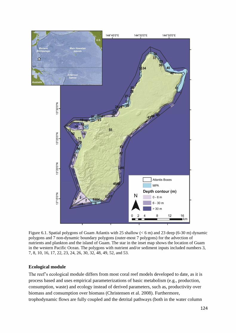
124
Figure 6.1. Spatial polygons of Guam Atlantis with 25 shallow (< 6 m) and 23 deep (6-30 m) dynamic
polygons and 7 non-dynamic boundary polygons (outer-most 7 polygons) for the advection of
nutrients and plankton and the island of Guam. The star in the inset map shows the location of Guam
in the western Pacific Ocean. The polygons with nutrient and/or sediment inputs included numbers 3,
7, 8, 10, 16, 17, 22, 23, 24, 26, 30, 32, 48, 49, 52, and 53.
Ecological module
The reef’s ecological module differs from most coral reef models developed to date, as it is
process based and uses empirical parameterizations of basic metabolism (e.g., production,
consumption, waste) and ecology instead of derived parameters, such as, productivity over
biomass and consumption over biomass (Christensen et al. 2008). Furthermore,
trophodynamic flows are fully coupled and the detrital pathways (both in the water column

125
and in the sediment layer) are explicitly modeled. To represent those pathways, we included
42 functional groups consisting of 3 detrital, 5 plankton, 3 algal, 3 sessile invertebrate, 7
mobile invertebrate and 20 vertebrate groups (Appendix A). To accommodate improved
understanding of reef resilience we grouped fishes by their life-history characteristics, habitat
preferences and diet in the following functional groups: piscivores, corallivores, invertivores,
planktivores, detritivores and herbivores. We have further classified the herbivores by their
ecological roles as excavators/bioeroders, scrapers, grazers and browsers (Bellwood and
Choat 1990, Paddack et al. 2006, Green et al. 2009, Hoey and Bellwood 2011, Heenan and
Williams 2013). Based on the biomass of each species in 2011 (Williams et al. 2012), we
took the weighted mean of species-specific data on diet and life-history parameters (e.g.,
growth rate, natural mortality, maximum age, age at maturity, size of recruits, length of
pelagic larval development, von Bertalanffy growth coefficients, swim speed) for the overall
estimation of those parameters for each functional group. Biomass estimates, spatial
distribution, and fisheries data are detailed further in Weijerman et al. (2014b).
We avoided aggregating fished and unfished species into the same functional groups,
and identified fishery target species based on shore-based creel surveys conducted since 1985
by Guam’s Division of Aquatic and Wildlife Resources (DAWR; Appendix A). We chose to
limit the fishery data to shore-based creel surveys and not include the boat-based creel
surveys as we assumed that the shore-based fishery took place entirely in our model domain
while the boat-based fishery is mostly focused on trolling and demersal fishing in deeper
waters. Appendix A has a complete list of the functional groups and their representative
species, i.e., species accounting for ≥ 75% of biomass per group for the fish groups based on
visual surveys conducted in 2011 by CRED (Williams et al. 2012). In addition to these living
and detritus groups, ammonia, nitrate, and silica are represented dynamically. The model’s
initial conditions represent 1985 (after a 10-year‘burn-in' phase) and we projected this
forward for 30–65 years under the set of scenarios described below.
The coral framework is the foundation for coral reef ecosystems; hence, corals are
integrally linked to most reef dynamics. Corals are consumers by night and photosynthesize
by day, but are also a source of food to corallivorous invertebrates and fishes. Due to their
three-dimensional structure, corals also provide habitat and shelter for many reef species
(DeMartini and Anderson 2007, Enochs and Hockensmith 2008). Even dead corals continue
to harbor diverse communities until erosion processes unbalanced by growth lead to the loss
of three-dimensional structure (Alvarez-Filip et al. 2009).
Coral species have different life history dynamics and sensitivities to environmental
factors (e.g., sediments, elevated temperature, disease) that influence mortality and growth.
Hence, we grouped corals into massive and encrusting corals (‘massive’)—with lower growth
rates and a lower sensitivity to stressors—and branching/tabular/columnar corals
(‘branching’)—with higher growth rates and higher sensitivity to stressors (Marshall and
Baird 2000, McClanahan et al. 2007).
After a literature review we identified key coral reef dynamics and the form of the
relationships for those dynamics and added corresponding code (Appendix F; Table F-1).
Coral specific parameters are included in Appendix G. We detailed the dynamics of coral
growth (and growth-related complexity) and competition with benthic algae that are
126
influenced by three main drivers (Fig. F-2): (1) climate change (a global stressor); (2) land-
based sources of pollution (a local stressor); and fishing activities (also a local stressor).
Table F-1 summarizes how these processes were simulated in the model and lists supporting
literature for these relationships. We acknowledge that we have captured only the main
processes, and that there are other processes which influence reefs that were either omitted or
represented only in a simplified way (e.g., symbionts’ dynamics [Baskett et al. 2009a],
microbe-induced coral mortality [Smith et al. 2006], coral and algal diseases [Aeby et al.
2011, Williams et al. 2014], linear relationship between herbivore size and bioerosion
[Mumby 2006] and others).
Model validation, verification and sensitivity analyses are discussed in Appendices
H–J. Of importance to note is that the effects of acidification are likely underestimated with
the model and coral biomass is sensitive to the growth rate of primary producers. Recently
the role of phytoplankton in structuring fish communities has received more attention and
helped explain the large regional (Pacific wide) differences in fish biomass between reefs
close to populated and unpopulated areas (Williams et al. 2015), corroborating the
importance of obtaining good estimates of these phytoplankton groups. Improving the
relationship between reef organisms and acidification or obtaining more accurate downscaled
time series of projected change in pCO2 and getting better growth rates and biomass estimates
of phytoplankton communities will likely enhance the model’s capabilities to make
projections. Additionally, the model skill in estimating fish biomass had a clear bias and
overestimated a number of groups. More research is necessary to explain the bias and then
correct for it (e.g., better fishery data, diet data of apex predators, recruitment data for the
overestimated fish groups). However, with the current information available it is possible to
make relative comparisons (Appendix F).
6.2.3 Model scenarios and model output
The outcome of a control run (Appendix H) that not included any of the identified stressors
was compared with outcomes from runs with the various added drivers: climate change (i.e.,
ocean warming and acidification), land-based sources of pollution (LBSP) and fishing.
Models were run for 30 years (1985–2015) to explore present conditions and for 65 years
(1985–2050) to explore future conditions.
Predicted changes in atmospheric CO2 concentrations came from the IPCC fifth
Assessment Report using the highest emission scenario, Representative Concentration
Pathway (RCP) 8.5 projection (Stocker et al. 2013). Predicted sea surface temperature data
also came from the RCP 8.5 projection using the HadGEM-AO model output (data
downloaded from the Coupled Model Intercomparison Project Phase5 [CMIP5]:
http://apdrc.soest.hawaii.edu/las8/UI.vm), as the historical 1985–1990 modeled data
corresponded well with satellite-derived SST data for Guam during the same time period. We
overlaid this trend on the existing time series of temperature from the CT-ROMS model
output (Castruccio et al. 2013) for each Atlantis polygon and created a projected temperature
time series for each polygon out to 2050 while maintaining spatial differences around Guam.
These increased CO2 concentrations for emission scenario RCP 8.5 led to a decrease
in the oceanic pH which in turn led to a reduction in the aragonite saturation state of the

127
ocean resulting in reduced calcification rates modeled as a reduced growth rate of corals
(Appendix F which also explains relationships between pH and several other organisms).
Land-based sources of pollution were modeled as additional input of nitrogen and
sediments into coastal polygons that had riverine runoff or sewage outflow pipes (Appendix
F, Weijerman et al. 2014b). The sediment and nutrient loads were based on data collected
from 2005–2007 (Guam Environmental Protection Agency, and CRED) and used as initial
condition input data for the model. River flow and additional nutrient and sediment input data
were based on time series from 1991 and 2011 and the last year was repeated for future
projections. Hence, changes in land-use or the amount of rain were not taken into account.
Fishing mortality was calculated for each functional group based on the historical catches
from shore-based creel surveys conducted by DAWR. We assumed fishing mortality stayed
constant at 2010–2012 levels for projections (Appendix F).
Ecosystem metrics used to score the effect size of the disturbances were based on
performance indicators for reef resilience (Bascompte et al. 2005, Bellwood et al. 2011,
Weijerman et al. 2013) plus one additional indicator: the ratio of biomass of targeted species
in the recreational reef fishery at the end relative to the start of a simulation (Table 6.1). We
used that metric as a proxy for one source of socio-economic benefits from the reef
ecosystem—availability of preferred target fishery species.
Table 6.1. Ecosystem metrics used to determine effect size of simulation of scenario runs.
Metric Description Rationale
Ratio of benthic
calcifiers to non-
calcifiers
Ratio of total biomass of corals and
crustose coralline algae (CCA), and
total biomass of turf and fleshy
macroalgae in the model domain
Corals form the framework of reef ecosystems
and CCA is the ‘glue’ that cements the reef
together a high ratio of calcifiers to non-
calcifiers implies a more structurally complex
system that provides more desirable ecosystem
services than a macroalgal-dominated (flat)
system (Weijerman et al. 2013)
Mean trophic level
of the community Biomass-weighted average of the
trophic level of all functional groups
in the ecosystem.
Indication of maturity for ecosystems; higher
value represents more ecosystems (Weijerman et
al. 2013)
Biomass of apex
predators Sum of biomass of apex predator
groups (sharks, roving piscivores,
benthic piscivores and mid-water
piscivores).
Indication of ‘health’ for ecosystems; higher
value represents ‘healthier’ ecosystem. In
general, more apex predators decrease
community susceptibility to perturbations
(Bascompte et al. 2005).
Biomass of
herbivorous fishes Sum of biomass of all herbivorous
fish groups. Indication of resilience with more herbivores
leading to less chance of ecosystem shifts to
undesirable algal-dominated state (Bellwood et
al. 2011).
Total biomass
(excluding detritus) Sum of biomass of all species. Indication of maturity/stability of ecosystems;
higher value represents more mature or stable
ecosystem (Weijerman et al. 2013)
Ratio of biomass of
target species at end
to start of a run
Total biomass of all fish species that
are targeted in the reef fishery at the
end vs start of simulation run.
Indicator of socioeconomic condition; higher
value means higher availability of target species
to recreational fisherman

128
Ecosystem metrics were calculated as the average over the last three years of a
simulation, to smooth over intra-and interannual variation, and results for each Atlantis
polygon were summed to get results for the entire model domain for the island of Guam. For
each of the six ecosystem metrics, the response ratio was calculated as the ratio of the metric
under a scenario (e.g., climate change) relative to the value of that metric in the control run,
following the methods in Kaplan et al. (2013). The interactive effects among the drivers were
explored to see if their combined effect led to higher values (positive interaction) or lower
values (negative interaction) than would be expected based on the sum of the impacts of the
individual drivers (Kaplan et al. 2013). To determine the interactive effect size another two
simulations were conducted: one with two drivers acting simultaneously (adding the two
stressors with the largest effects individually), and the other with all three drivers. For
instance, if two drivers individually caused a 2% and 3% decline in a metric, the additive
expectation of combining both drivers is a 5% decline. If simultaneously applying the drivers
actually led to only a 4% decline, the interaction is slightly positive; if simultaneously
applying the drivers led to a 6% decline, the interaction is slightly negative. Based on the
assumption that the sum of the individual effects is simply additive, the difference between
the results of the simulation with concurrent drivers and the simulation results of the two or
three individual drivers should be zero. To determine this interactive effect size, d, we added
the relative control value (always 1 because results are standardized to the control) to the
result of the scenario run with two or three drivers acting concurrently, and subtracted the
individual effect sizes of the drivers according to:
d1,2, = YAB +Ycontrol – YA – YB
d1,2,3 = YABC +2Ycontrol – YA – YB – YC
where YAB is the value of the ecosystem metric resulting from having two interactive drivers
acting concurrently and YABC is the ecosystem metric resulting from three interacting drivers.
A, B, and C are the three drivers (climate change, LBSP, and present day fishery). Ycontrol is
the relative control value (with the coefficient 2 to ensure that the expected interaction d is 0
if effects are simply additive), resulting from a simulation of the control run, and YA, YB, and
YC indicate the value of the simulation of just the one driver.
6.3 Results
6.3.1 Individual drivers
Among the three 30-year (1985–2015) single stressor scenarios, fishing clearly had the
largest overall ecosystem impacts based on the performance metrics used, mostly due to the
large negative effect on the biomass of apex predators and the start-to-end ratio of biomass of
fish groups targeted by recreational fisherman (Fig. 6.2). Global climate change almost
exclusively affected the ratio of calcifiers to non-calcifiers resulting in a shift from coral and
crustose coralline algae to turf and macroalgae (Fig. 6.2). LBSP had the largest effect on the
ratio of calcifiers vs. non-calcifiers as well as clear effects on the biomass of apex predators.
Trophic level was least affected of the ecosystem metrics, possibly because of the taxonomic
resolution of the model; target and non-target groups had similar trophic levels and the
biomass of apex predators was low in all simulations (e.g., 14% in the control scenario)

129
compared to the biomass of the other fish groups, so even the 35% reduction in apex predator
biomass due to fishing and 18% reduction due to land-based sources of pollution did not have
a great influence on the overall trophic level of the community.
Figure 6.2. Response ratio of individual drivers’ effect to control effect of the six ecosystem metrics
after 30-year simulations. Responses greater than the control indicate a positive effect, and responses
smaller than the control indicate a negative effect. The control simulation had no external drivers.
LBSP is land-based sources of pollution. Climate change represents a simulation of both ocean
warming and acidification. Fishing was simulated using a fixed fishing mortality based on 2010–2012
shore-based fishery landings.
Climate change effects dominate model dynamics at longer time scales (65 year
simulations, 1985-2050). Using projected sea surface temperature rises, the bleaching
threshold would be exceeded every year from 2023 onwards (Appendix F, year 48 in Fig. F-
4). Therefore, it is not surprising that the effects of climate change are extremely high for the
calcifiers to non-calcifiers ratio (ratio = 0.24 in climate change scenario versus 1.33 in
control). In this longer simulation, climate change also had a negative effect on total biomass,
including a decrease in most prey species other than some of the herbivorous fishes (Fig. 6.3).
Similar to the 30-year simulation, fishing affected almost all ecosystem metrics negatively,
but particularly the biomass of apex predators and target fishes (Figs. 6.3 and 6.4).

130
Figure 6.3. Response ratio of individual drivers’ effect to control effect of the six ecosystem metrics
after 65-year simulations. Responses greater than the control indicate a positive effect, and responses
smaller than the control indicate a negative effect. The control simulation had no external drivers.
LBSP is land-based sources of pollution. Climate change represents a simulation of both ocean
warming and ocean acidification. Fishing was simulated using a fixed fishing mortality based on
2010–2012 reef-fish fishery landings.
Among the modeled vertebrate groups, turtles and mid-water piscivores came out as
‘winners’ under the fishing scenario (Fig. 6.4), as their predators, sharks, declined, and, in the
case of turtles, competition for food (algae) also declined.
Averaging all metrics (Fig. 6.5) emphasizes that climate change is the dominant driver
over the long term (65-year projections through year 2050), while fishing and LBSP appear
to have influenced the performance of the system (as measured by our ecosystem metrics)
most in the last 30 years (to 2015).
Figure 6.4. Vertebrate biomass response to each of the three simulated drivers, relative to the control
biomass. Biomass responses are end values for year 2050 (65 year run). Control is a simulation with
no external drivers. LBSP means land-based sources of pollution. Climate change represents a
simulation of both ocean warming and ocean acidification. Fishing is simulated with fixed fishing
mortality based on 2010–2012 shore-based fishery landings.
-0.9
-0.8
-0.7
-0.6
-0.5
-0.4
-0.3
-0.2
-0.1
0
0.1
calcifiers :non-calcifiers
trophic levelcomm.
biom. apexpred.
biom.herbivores total biom.
BYear65 :BYear0 target
groups
Re
spo
nse
rat
io
Climate change LBSP Fishery

131
Figure 6.5. Average response ratio across all six ecosystem metrics of climate change, land-
based sources of pollution (LBSP), and fishing after 30 (grey bars) and 65 (black bars) years.
Values equal to one indicate no change relative to the control simulation and values lower
than one indicate a negative effect. All six metrics were weighted equally.
6.3.2 Concurrent drivers
For the present-day conditions (30-year simulation), fishing appeared to have the greatest
impact followed by LBSP (Fig. 6.5). Simulating those two drivers concurrently showed slight
positive interactions for five out of six ecosystem metrics, i.e., the combined effects of
concurrently simulating the two drivers were more positive than the additive effects of the
two individual drivers. That was also true in simulations of all three drivers concurrently (Fig.
6.6), but in both cases these antagonistic effects were ≤0.10. Note that strong declines in the
ecosystem metrics were still observed in scenarios with concurrent drivers, for instance the
biomass of apex predators declined to only 55% of the value under the control scenario.
Figure 6.6. Interactive effect size on six ecosystem metrics (x-axis) when simulating fishing and
LBSP concurrently (two drivers) and all three drivers (also including climate change) at the end of a
30-year run. The difference between the expected effect size, if these were simply additive, and the
actual effect size of simulations with the two or three drivers concurrently is indicated by the black
and grey bars respectively.
For the 65-year simulation, climate change had the largest individual effect followed
by fishing and LBSP (Fig. 6.5), so we simulated those two drivers concurrently first, and then
simulated all three drivers concurrently. Just as in the 30-year simulation, the interactive
effect size was mostly positive, especially when all three drivers acted concurrently, i.e., a

132
scenario with concurrent drivers led to slightly higher values of ecosystem metrics than could
have been predicted from simply adding the individual driver effects (Fig. 6.7). As with the
30-year simulation, despite the slight positive interactions of the concurrent drivers, actual
effects were negative, just not as extreme as might be expected by summing the individual
driver effects. For instance, despite the 0.21 positive interaction of the ratio of calcifiers:non-
calcifiers (Fig. 6.7), the combination of three drivers drove this ratio to only 19% of the
control scenario result; the ratio of calcifiers to non-calcifiers was 0.24 if just climate change
was simulated and 1.40 if just fishing was simulated, suggesting that the benefits of fishing
for this metric were not fully realized when combined with climate change.
Figure 6.7. Interactive effect size on six ecosystem metrics (x-axis) when running simulation with
climate change and fishery concurrently, and all three drivers at the end of a 65-year simulation. The
difference between the expected effect size, if these were simply additive, and the actual effect size of
simulations with the two or three drivers is indicated by the black and grey bars respectively.
In terms of management applications of these model results, reducing LBSP appears
to have a noticeable effect on coral biomass, giving corals some additional capacity to deal
with the early effects of climate change under the RCP 8.5 scenario for CO2 emissions.
However, when ocean temperature exceeds the bleaching threshold every year, the prognosis
for corals is bleak (Fig. 6.8). Our study indicates that when just fishing is restricted, coral
biomass follows the same trend as under a status quo scenario (Fig. 6.8).
The trend for the biomass of apex predators and of herbivores, showed, not too
surprisingly, that the no-fishing scenarios (short dashed and dotted lines) resulted in the
highest fish biomass. Similar results were obtained for the relative change in biomass of
target species compared to the initial biomass: a declining and stabilizing trend at around
53% of initial biomass for status quo and at 55% for no LBSP scenarios and stabilizing at
80% for no fishing and at 85% for no fishing and no LBSP scenarios. What was surprising
though, is that the herbivorous fish biomass stayed stable despite the reduction in coral
biomass (and hence structural complexity and hiding places) in the last 15 years (Fig. 6.9).
However, a 110-year simulation (only simulated for status quo scenario) does indicate that
the biomass of the herbivorous prey fish slowly declines after coral cover has declined with a
lag-time of about 15 years (Fig. 6.10). These 15 years correspond well to their mean
generational age-span of 12.3 (SD 6.4) years.

133
Figure 6.8. Projected effects of climate changes (RCP 8.5 scenario for pCO2 emissions) concurrent
with local threats (LBSP [land-based sources of pollution] and fishing) on massive (top red-shaded
lines) and branching (bottom blue-shaded lines) coral biomass. The result of a no fishing scenario
corresponded with the status quo scenario for both coral groups and was left out for clarity.
Figure 6.9. Projected effects of predicted climate changes (RCP 8.5 scenario for pCO2 emissions)
concurrent with local threats (LBSP [land-based sources of pollution] and fishing) on biomass of
herbivorous fish (top green-shaded lines) and apex predators (bottom purple-shaded lines).
Figure 6.10. Projected effects of predicted climate changes (RCP 8.5 scenario for CO2 emissions)
concurrent with local threats on biomass of herbivorous fish (green line) and apex predators (purple
dashed lines).

134
Main ‘winners’ projected by the model at the end of this century under a status quo
scenario with climate change were turtles (100% increase), benthic filter feeders (600%
increase) and detritivorous invertebrates (300% increase; Fig. 6.11).
Figure 6.11. Projected relative biomass after a 110 year simulation comparing 2095 (end of
simulation) to 2015 for (top panel) vertebrate and (bottom panel) invertebrate functional species
groups.

135
6.4 Discussion
Ecosystem-based management considers the indirect and cumulative effects of multiple
threats to a system. Ecosystems can frequently recover from short-term low-intensity
disturbances, but when disturbances occur too frequently or when multiple disturbances
impact the system in a short time span (i.e., before the system is recovered), recovery is
limited or may not happen at all (Paine et al. 1998, Edwards et al. 2011, Ban et al. 2014).
Quantifying the interactive effect size of disturbances is one way to gain insight into how
these disturbances cumulatively affect the ecosystem. Looking first at the disturbances
individually, ocean warming and acidification, had the largest effect on the ecosystem
compared to LBSP and fishing, with fishing being a close second when looking at the end of
65-year simulations. Whereas ocean change primarily affected the benthic reef community,
fishing impacted all ecosystem metrics, including four out of six, negatively. Fishing had the
strongest negative effect on the biomass of target species and apex predators. This result is
expected from any selective fishery (Jennings and Polunin 1996, Friedlander and DeMartini
2002). Surprising was the result that fishing actually had a beneficial effect on the ratio of
calcifiers to non-calcifiers. This positive effect could be explained by the projected increase
in turtle biomass, which were less preyed upon as the shark (main predator) populations had
declined, and by less bioerosion, especially from large parrotfishes.
Results also suggest that presently (end of 30-year simulation) fishing affected almost
all ecosystem metrics negatively and that LBSP exacerbated this effect, but not quite as badly
as would be expected under additive assumptions. In the case herbivore biomass, fishing had
a negative effect, but LBSP had a slight positive effect. The scenario with those concurrent
drivers led to a slightly lower value of that ecosystem metric than could have been predicted
from simply adding the individual driver effects. This result could indicate that the input of
nutrients and sediments, which led to an increase in food abundance, offset the reduction in
herbivore biomass through their extraction due to fishing. This pattern also held up after
simulating concurrently the third driver, climate change. Despite the low interactive value,
the combination of two and three drivers drove the herbivore biomass to 84% of the value in
the control scenario.
Cumulative effects of combining all three drivers in the 65-year simulation were
negative, in correspondence with temperate fisheries systems where the ecosystem was worse
off once all three drivers came into play (Kirby et al. 2009, Ainsworth et al. 2011b).
Estimated interactions were slightly positive, meaning that the combined effects were only
slightly less than a null assumption of summing the individual effects of each of the three
drivers.
As some studies speculated that mitigating local stressors to reefs increases the coral’s
resilience to climate change (Hughes et al. 2010, Edwards et al. 2011, Pandolfi et al. 2011,
Kennedy et al. 2013), we simulated (1) a scenario with climate change and no input of LBSP,
(2) a scenario with climate change and no fishing, and (3) a scenario with climate change and
no local drivers (no fishing and no LBSP) and compared coral biomass trajectories with a
status quo scenario (including climate change and local drivers). Model outcomes showed
that when LBSP was stopped, coral biomass increased and stayed higher longer compared to
the status quo scenario. In contrast to the idea that a fishing moratorium could mitigate the

136
decline in coral biomass, our study suggests that this increasing trend in coral biomass was
only slightly improved when fishing was also stopped. This result was also seen in a study in
the Indian Ocean where fishery closures did not change hard coral cover (McClanahan 2014).
Indeed, we showed that the biomass of herbivores and apex predators increases when fishing
is stopped, however, despite the lower biomass of herbivores under the fishing scenario, coral
biomass is higher and algal biomass is lower compared to the no fishing scenario.
Though studies (Mumby and Harborne 2010, Edwards et al. 2011) showed that high
herbivore populations are important for the recovery of coral populations in some situations,
our results do not suggest that this provides a substantial buffer against climate change for
coral cover in Guam. Indeed, a study in the Caribbean (Edwards et al. 2011), the Great
Barrier Reef (Thompson and Dolman 2010), and a global meta-analysis (Selig et al. 2012)
showed a similar demise of coral cover when bleaching events were taken into account
despite the establishment of MPAs. In the Caribbean study, depending on the location, a high
presence of herbivores did postpone the most detrimental effects of ocean warming on coral
cover by 18–50 years (Edwards et al. 2011). This discrepancy in the influence of herbivores
could be caused by the way herbivore populations were modelled. In the Edwards et al.
(2011) model, grazing intensity was fixed as 40% in the high grazing scenario and contrasted
with a 10% grazing term in the low grazing scenario. In our model, although the total
biomass of herbivores was lower in the status quo scenario, the grazing intensity appeared to
still be high enough to keep the biomass of macroalgae down and of corals up. Model skill
results (Appendix F) showed that the model over-estimates some herbivorous fish groups,
most notably the small-bodied parrotfish. This over-estimation of small-bodied parrotfish
may contribute to our projection of the relatively weak fishing effects on coral biomass.
Our results indicate that water quality is a key local threat in the decline of coral
biomass. Improving the water quality might delay the coral’s ultimate climate-driven decline
by 5–8 years, which could buy time to acclimate to higher temperatures. A study on the coral
genus Pocillopora from Guam suggested that corals can, at least in part, acclimate to
temperatures of 32°C which would be sufficient for persistence under the RCP 8.5 scenario
(Rowan 2004). If corals cannot acclimate over such short time spans (5–8 years) and we
experience the RCP 8.5 pathway, our model suggests that reef-building corals will be
severely impacted by 2035–2040 (Fig. 6.8). This result is similar to a more general modelling
result from Pacific reefs where coral cover dropped to 5% by the year 2050 and close to zero
in the year 2055 (Ortiz et al. 2014). Ortiz et al. (2014) suggested that corals in the Pacific
could recover if we can reduce to the RCP 2.6 low CO2 emission scenario.
With the reduction of the structural framework of a degraded coral reef, after a time
lag of about 15 years, the biomass of herbivorous fish declined. This time lag is in between
those observed in the western Indian Ocean (5–10 years; Graham et al. 2007) and the
Caribbean (25–30 years; Paddack et al. 2009). In general, roving herbivores, such as,
surgeonfishes and parrotfishes, can increase in abundance after mass bleaching events (Baker
et al. 2008), but their recruits are dependent on coral habitat and are responsible for the lag-
time effect in the ultimate decline in population size (Graham et al. 2007). Indirect effects of
coral loss also include an abundance of sponges (Loh et al. 2015) and a decrease in reef fish,
mostly obligate corallivorous species, pomacentridae and gobies (Coker et al. 2014). Our

137
study showed that benthic filter feeders (including sponges) had doubled in biomass whereas
sea stars (including the corallivorous crown-of-thorns seastars) declined. Corallivorous fish
did not decline but, in fact, increased. This increase is likely because the modeled
corallivorous fish functional group included species that also feed on soft coral and sponges.
Similarly, the functional group planktivores (including pomacentrids) were not restricted to
the small planktivores that are always associated with (mostly branching) corals, but also
included large-bodied species, for example, unicorn fishes, resulting is less of a decline that
would be expected from truly reef dependent species (Fig. 6.11; Wilson et al. 2006, Baker et
al. 2008).
6.5 Concluding remarks
We successfully developed an integrated coral reef ecosystem model that takes into account
the key reef dynamics and their relationship to disturbances. The model simulations of these
dynamics corresponded well with empirical data from around Guam and regional studies.
The model would, however, still benefit from further refinement. In particular, fishery data,
and the nutrient, phytoplankton, and zooplankton dynamics could be improved, as should the
handling of vertical mixing. Such refinements, however, would unlikely change our results
on the short- and long-term importance of the different drivers examined.
Quantifying an ecosystem models’ uncertainty and performing skill assessments are
still an under-studied part of ecosystem modelling partly because of the complexity (and
hence long run times and large number of parameters) of ecosystem models that
computationally prohibits the use of well-established statistical analyses. Naturally, however,
those results would greatly enhance the models’ robustness and management applicability.
By providing insights within a consistent setting, this version of the Guam Atlantis model can
be used as a decision-support tool to quantify the relative tradeoffs of alternative ecosystem-
based management scenarios. Guam Atlantis is capable of simulating the consequences of
different management strategies (e.g., reduction in land-based sources of pollution or
fishing), while simultaneously allowing for the expected effects of ocean warming and
acidification, and therefore has utility for a range of regional (e.g., regulating pollution, land
use and fisheries) and global (e.g., world-wide mitigations of CO2 and other greenhouse
gasses) management applications.
Simulating the main stressors on coral reef ecosystems suggests that the reefs around
Guam are presently predominantly affected by fishing and secondarily by the input of
nutrients and sediments. In the near future (20–30 years from now), the predicted climate
change will have the most profound effect on coral reefs. Reducing additional nutrients and
sediments could mitigate the loss of coral biomass for 5–8 years, but once the temperature
exceeds the bleaching threshold annually, corals are unlikely to survive. A consequence of
the loss of corals is the slow decline in fish abundance, particularly of those that use the
corals as habitat during a part of their life cycle, and this decline could impact the reef-fish
fishery negatively.

138
A sign advocating the stop of night-time spear fishing. NOAA photo

139
Chapter 7
Management Strategy Evaluation applied
to coral reef ecosystems in support of
Ecosystem-based Management
Weijerman, M, Fulton, EA, Brianard RE. 2015. Submitted to Ecography. Management
Strategy Evaluation applied to coral reef ecosystems in support of Ecosystem-based
Management.

140
Ecosystem modelling is increasingly widely used to explore ecosystem-level
effects of changing environmental conditions and management actions. For
coral reefs there has been a push in recent decades toward the use of
ecosystem models to evaluate effects of fishing and the efficacy of marine
protected areas as. We applied an ecosystem model to the coral reef
ecosystem of Guam using a suite of management scenarios prioritized in
consultation with local resource managers to review the ecological and socio-
economic performance of the reef-fish fishery including secondary effects to
coral habitat. Comparing tradeoffs across the selected scenarios showed that
each scenario performed best for at least one of the selected performance
indicators. The integrated ‘full regulation’ scenario (size limits, catch limits,
marine preserves and no additional land-based sources of pollution)
outperformed other scenarios with four out of the six performance metrics at
the cost of reef-fish landings. When the effects of climate change were taken
into account, several scenarios performed fairly equally well, but none
prevented a collapse in coral biomass over the next few decades assuming a
business-as-usual greenhouse gas emissions scenario.
141
7.1 Introduction
Sustainable use of environmental resources is inextricably linked to long-term human well-
being. However, there is overwhelming evidence of anthropogenic loss or degradation of
coral reef ecosystems worldwide (Gardner et al. 2003, Paddack et al. 2009, Brainard et al.
2011, Burke et al. 2011, De’ath et al. 2012). Coral reef managers are challenged with
sustaining the ecosystem functions and services under changing environmental conditions
and use patterns (Moberg and Folke 1999, Riegl et al. 2013, McClanahan et al. 2014).
Management decisions intended to achieve desired outcomes for marine systems have
cultural, social, and economic consequences for the many people who depend on or use those
systems. Those consequences should be accounted for in ecosystem status assessments
(Brewer et al. 2012, Plagányi et al. 2013, Cinner 2014, Pratchett et al. 2014). Over around the
last decade there has been a movement toward ecosystem-based management (EBM) and
ecosystem-based fisheries management (EBFM) and growing recognition that human
dimensions are an integrated part of these ecosystems (Pikitch et al. 2004, Fulton et al.
2011c). This move towards EBM and EBFM has also been seen in ecosystem model-based
applications for coral reef ecosystems, where coastal communities are often dependent on the
reef’s resources (Wilkinson 2008) making ecosystem models an important tool in evaluating
ecological and socioeconomic tradeoffs of management policies (McClanahan et al. 2006,
Ainsworth et al. 2008a, Brown and Mumby 2014).
A recent literature review showed there has been a steep increase in the number of
peer-reviewed articles on artisanal coral reef fisheries in the last 30 years (Johnson et al.
2013). In 80% of 464 peer-reviewed articles on coral reef fisheries management implications
of alternative management scenarios were discussed, but primarily in general conjectural
terms (Johnson et al. 2013). Only 22% of these studies presented recommendations based on
their own research. Studies on the effectiveness of different management actions and
approaches, tradeoffs and trajectories under climate change are still lacking (Johnson et al.
2013) and this study contributes to filling that gap.
In this paper, we describe the application of an ecosystem model to a complex
multispecies fishery with degraded habitats accounting for the effects of climate change. We
apply the model using the island of Guam in the tropical west Pacific Ocean as a case study.
We use the Atlantis ecosystem model (Fulton 2001, http://atlantis.cmar.csiro.au/) that has
previously been applied to various, primarily temperate and polar, marine ecosystems around
the world to explore ecological questions, impacts of ocean and climate change, spatially-
explicit fishing efforts and to rank alternative management and policy scenarios (Fulton et al.
2011b). This is the first published application of Atlantis for a coral reef ecosystem
(Weijerman et al. 2014b). Five management scenarios selected during workshops in Guam
were compared against the status quo i.e., maintain existing Marine Protected Areas (MPAs)
and current levels of land-based sources of pollution (LBSP): A) remove existing MPAs and
implement catch limits (TAC), B) remove MPAs and implement minimum-size limits; C)
remove MPAs and implement TAC and size limits; D) status quo with no LBSP; and E) size
limits and TAC and no LBSP. For completeness we also examined an integrated scenario F)
all regulations in place, i.e., scenario E with MPAs. Scenarios were simulated with and
without including climate change predictions.

142
7.2 Methods
7.2.1 Study site
Over the last three decades coral cover and reef-fish biomass have declined in Guam
(Burdick et al. 2008). To enhance conservation of fish stocks and habitat, the government of
Guam established five marine preserves. MPAs have been shown to be effective at enhancing
resilience to climate change (Micheli et al. 2012), increasing coral recovery in the Caribbean
(Mumby and Harborne 2010), supporting larval supplies to other areas (Christie et al. 2010)
and enhancing biomass and reproduction of fish species (Evans et al. 2008). The MPAs
around Guam have increased fish abundance and reproduction of some fish species compared
to the open access areas (Taylor et al. 2012, Williams et al. 2012). Managers are now
interested in using ecosystem modelling to explore tradeoffs of alternative management
approaches (Weijerman and Brown 2013). In two workshops held in Guam in November
2012 and June 2014, resource managers and other stakeholders were asked to select
management approaches and objectives that were of interest. The resulting overarching goal
for coral reef management was “to obtain a sustainable coral reef ecosystem that can achieve
and maintain a more desirable state than the current state given local stressors (e.g., fishing,
land-based sources of pollution, COTS predation) and climate-related stressors (ocean
acidification and warming).” Specific objectives necessary to achieve that goal provide target
outcomes that we used to assess the effectiveness of different modeled management
scenarios. These were: (1) improved water quality (no additional LBSP), (2) increased reef
resilience, (3) enhanced fish biomass, and (4) similar or improved fisheries landings
(Weijerman and Brown 2013). These objectives have two somewhat contradictory elements:
improved ecosystem status or condition (objectives #1–3) at the same time as sustained or
increased levels of extraction (objective #4).
7.2.2 Atlantis ecosystem model
The Atlantis ecosystem modelling framework is a spatially-explicit dynamic model that
couples biophysical processes with human-use dynamics and the adaptive management cycle.
The biophysical module tracks nutrient flows (mainly nitrogen and silica) through the
biological and detritus groups specified within the model domain (Fulton 2001). Production,
consumption and growth, habitat dependency, reproduction, movement and large-scale
migration are all handled explicitly. All vertebrates are represented as age-structured groups;
invertebrates are handled as biomass pools. Apart from these living groups, ammonia, nitrate,
silica, carrion, and labile and refractory detritus are also dynamically modeled in the water
column and sediment. Human-use dynamics can be incorporated through the fishing, and
management and assessment modules. For the purpose of our paper, fishing was represented
by constant fishing mortality and we did not include the management and assessment module.
The Guam Atlantis model encompasses the shallow (< 30 m) reefs around Guam,
spanning approximately 110 km2 (Fig. 7.1). This model domain is divided into 55 marine
spatial zones with one or two water layers and is forced with daily hydrodynamic flows,
salinity, and temperature outputs from a 5-km resolution, three-dimensional Regional Ocean

143
Modelling System model (www.myroms.org) developed for the Coral Triangle region in the
western Pacific Ocean (Castruccio et al. 2013).
Trophic dynamics are represented by 42 functional groups based on diet, life-history,
ecological role, and habitat requirements. Where appropriate, functional groups were further
divided into target and non-target taxa (Appendix A). Initial biomass estimates for all groups
came from the Pacific Islands Fisheries Science Center, Coral Reef Ecosystem Division
supplemented with data from the Guam Coastal Zone Management Program, Guam Division
of Aquatic and Wildlife Resources (DAWR), Guam Environmental Protection Agency, and
the University of Guam Marine Laboratory and represent the ecosystem status over the
period 2009–2011 (Weijerman et al. 2014b).
Climate change effects, through ocean acidification and ocean warming, are included
in the model (Chapter 6). Ocean acidification negatively affected growth rates of corals as
well as echinoderms, molluscs, crustose coralline algae and copepods (modeled as
herbivorous zooplankton), and increased the growth rates of phytoplankton and macroalgae
(Langdon 2002, Cohen and Holcomb 2009, Kroeker et al. 2010, Shaw et al. 2012). Predicted
atmospheric CO2 data came from the Intergovernmental Panel on Climate Change
Assessment Report 5 using the highest emission scenario Representative Concentration
Pathway (RCP) 8.5 projection. These time series data were read into Atlantis to calculate the
change in pH and aragonite saturation state and, ultimately, therefore calcification rates of
corals and other calcifiers (Langdon and Atkinson 2005, Feely et al. 2009, Anthony et al.
2011b). Effects of ocean warming included coral bleaching (the expulsion of symbiotic algae
in the coral tissue) leading to lower coral growth rates and higher mortality. Bleaching events
were triggered when ocean temperature exceeded the local bleaching threshold (1°C above
the maximum summer temperature in Guam) for more than specified periods of time (known
as ‘degree heating weeks’ [DHW] that includes the magnitude and duration of elevated
temperatures): 3 DHW for branching corals and 4 DHW for massive corals (Jokiel and Coles
1990, McClanahan 2004, Donner et al. 2005). Predicted sea surface temperature data came
from the RCP 8.5 projection using the HadGEM-AO model output, which has been shown to
perform well compared to 20 similar models from the Coupled Model Intercomparison
Project Phase5 [CMIP5] (CRED unpublished data)(data downloaded from:
http://apdrc.soest.hawaii.edu/las8/UI.vm). We overlaid this trend on the existing time series
of temperature (Castruccio et al. 2013) for each Atlantis polygon to maintain spatial
differences around Guam and create a time series out to 2047 (Fig. 7.2).

144
Figure 7.1. Spatial structure of the Guam Atlantis model based on homogeneous biophysical
characteristics. Polygons closest to shore have one depth layer (0-6 m) and the others two (0–6 m and
6–30 m for the middle ones and 0–6m and 6–100 m for the 7 outer, boundary polygons). Blue
polygons indicate marine preserves. The star in the inset map represents the location of Guam and the
Mariana Archipelago in the Pacific Ocean. The polygons with nutrient and/or sediment inputs
included numbers 3, 7, 8, 10, 16, 17, 22, 23, 24, 26, 30, 32, 48, 49, 52, and 53.

145
Figure 7.2. Trajectories of (top) predicted pCO2 (IPCC AR5 RCP8.5) and (bottom) sea-surface
temperature (HadGEM-AO) with bleaching threshold at 30.1°C (red dashed line). Time line is from
1975–2047. These time series were used as forcing factors for future climate and ocean change.
Initial conditions for the model and a detailed description of the model development
and data sources are given in Chapters 4 and 6. The model was considered robust after
passing three calibration tests (Horne et al. 2010, Link et al. 2010, Ainsworth et al. 2011a):
(1) the model was able to reproduce unfished biomasses, i.e., the model reached and
stabilized at similar biomass levels to those observed in marine reserves in Guam and at
unpopulated Northern Mariana Islands; (2) weight-at-age stayed stable and abundance of size
classes decreased with increasing size classes (few large organisms and many small ones),
and (3) the model was able to fit historical catch time series which were derived from inshore
creel fishery surveys conducted by DAWR. The model was further validated by comparing
model output data for key coral reef dynamics (effect of LBSP, mitigating effect of structural
complexity on fish predation, coral-algal competition) with empirical data from Guam and
published relationships (Appendix F).
7.2.3 Simulated management scenarios
In total, seven scenarios were simulated with Guam Atlantis:
1) Status quo represented by five MPAs and existing levels of land-based sources of
pollution. The status-quo simulation had constant fishing mortalities per functional group
with no fishing in the MPAs. Fishing mortalities were calculated using shore-based creel
surveys (DAWR) extrapolated to the whole of Guam by staff from the NOAA Western
Pacific Fisheries Information Network (WPacFIN). Annual catches were compared to
estimates of standing stocks for each functional group to give fishing mortality rates. We
used a constant fishing mortality (F) per functional group (Table 1) with F=0 per year in
the five MPAs. LBSP was modeled as the addition of nutrients and sediments to the
coastal polygons with riverine run-off and/or sewage outfall pipes (Fig. 7.1), and estimated

146
loads were based on flow data and the related sediment and nutrient inputs per river for
each Atlantis polygon (Weijerman et al. 2014b).
2) Remove existing MPAs and implement a weekly catch limit (TAC) with existing levels of
LBSP. We estimated an annual limit as 75% of the average catches of the first five years
of the status quo catches and then converted this value to a weekly TAC. We simulated the
TAC scenario with the same fixed fishing mortalities as in the status quo simulation.
Fishing was allowed in every polygon, when the TAC was reached, fishing stopped for
that week.
3) Remove existing MPAs and implement size limits with existing levels of LBSP. For the
size-limits based fishery simulations, we assumed a fishery that would leave all immature
fishes. Based on the weight and age at first maturity, the fishery start age for each
functional group differed (Table 7.1). Fishing was allowed in every polygon with fixed
fishing mortalities equal to the status quo simulation.
4) Remove existing MPAs and implement TAC and size limits with existing levels of LBSP.
In this scenario we combined the rules of scenarios 2 and 3.
5) Remove existing MPAs and implement TAC and size limits with no LBSP. This scenario
differed only from scenario 4 by not simulating the delivery of additional nutrients and
sediments to the coastal areas.
6) Status quo with no LBSP. In this scenario we used the same constant fishing mortalities as
identified under scenario 1, but did not simulate any additional LBSP to the coastal areas.
7) Full regulations: keep existing MPAs and implement size limits and TAC with no LBSP.
This scenario combines scenarios 5 and 6.
Each of the scenarios was first simulated for 30 years (1985–2015) without including
climate change predictions. Then, based on performance evaluation (see Results section), the
best three scenarios (#5–7) were also run for 45 years (1985–2030) under the current
trajectories for climate change (RCP 8.5).
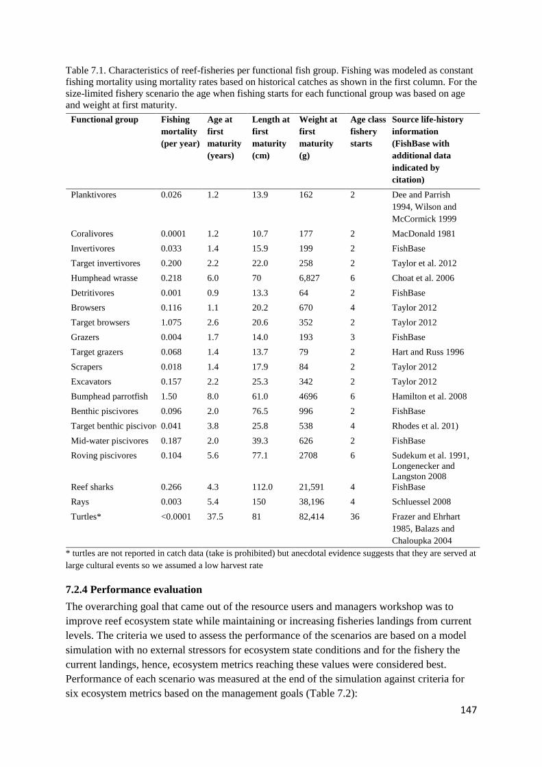
147
Table 7.1. Characteristics of reef-fisheries per functional fish group. Fishing was modeled as constant
fishing mortality using mortality rates based on historical catches as shown in the first column. For the
size-limited fishery scenario the age when fishing starts for each functional group was based on age
and weight at first maturity.
Functional group Fishing
mortality
(per year)
Age at
first
maturity
(years)
Length at
first
maturity
(cm)
Weight at
first
maturity
(g)
Age class
fishery
starts
Source life-history
information
(FishBase with
additional data
indicated by
citation)
Planktivores 0.026 1.2 13.9 162 2 Dee and Parrish
1994, Wilson and
McCormick 1999
Coralivores 0.0001 1.2 10.7 177 2 MacDonald 1981
Invertivores 0.033 1.4 15.9 199 2 FishBase
Target invertivores 0.200 2.2 22.0 258 2 Taylor et al. 2012
Humphead wrasse 0.218 6.0 70 6,827 6 Choat et al. 2006
Detritivores 0.001 0.9 13.3 64 2 FishBase
Browsers 0.116 1.1 20.2 670 4 Taylor 2012
Target browsers 1.075 2.6 20.6 352 2 Taylor 2012
Grazers 0.004 1.7 14.0 193 3 FishBase
Target grazers 0.068 1.4 13.7 79 2 Hart and Russ 1996
Scrapers 0.018 1.4 17.9 84 2 Taylor 2012
Excavators 0.157 2.2 25.3 342 2 Taylor 2012
Bumphead parrotfish 1.50 8.0 61.0 4696 6 Hamilton et al. 2008
Benthic piscivores 0.096 2.0 76.5 996 2 FishBase
Target benthic piscivores 0.041 3.8 25.8 538 4 Rhodes et al. 201)
Mid-water piscivores 0.187 2.0 39.3 626 2 FishBase
Roving piscivores 0.104 5.6 77.1 2708 6 Sudekum et al. 1991,
Longenecker and
Langston 2008 Reef sharks 0.266 4.3 112.0 21,591 4 FishBase
Rays 0.003 5.4 150 38,196 4 Schluessel 2008
Turtles* <0.0001 37.5 81 82,414 36 Frazer and Ehrhart
1985, Balazs and
Chaloupka 2004
* turtles are not reported in catch data (take is prohibited) but anecdotal evidence suggests that they are served at
large cultural events so we assumed a low harvest rate
7.2.4 Performance evaluation
The overarching goal that came out of the resource users and managers workshop was to
improve reef ecosystem state while maintaining or increasing fisheries landings from current
levels. The criteria we used to assess the performance of the scenarios are based on a model
simulation with no external stressors for ecosystem state conditions and for the fishery the
current landings, hence, ecosystem metrics reaching these values were considered best.
Performance of each scenario was measured at the end of the simulation against criteria for
six ecosystem metrics based on the management goals (Table 7.2):

148
1) Improved water quality. The metric used to assess the performance of this goal was
benthic calcifiers to non-calcifiers ratio with calcifiers defined as corals and crustose-
coralline algae (CCA) and non-calcifiers as turf and macroalgae. High concentrations of
sediments and nutrients favor macroalgal growth over coral growth influencing the
physical and ecological controls of coral-macroalgal dynamics (Hughes 1994, Lapointe
1997, Mumby et al. 2007a). Additionally, terrigenous sediment smothers corals and other
substrate thereby lowering coral growth and recruitment (Marshell and Mumby 2012).
Reefs in the southern part of Guam have experienced high sediment concentrations for
around the last 30 years, because of clearing and burning of upslope watersheds, and the
steep slopes wash large volumes of sediment into nearshore waters during heavy rainfall
events (Wolanski et al. 2003a, Wolanski et al. 2004, Burdick et al. 2008). Over the same
time period, severe recruitment failure has been observed (Minton et al. 2007). An
important function of corals and crustose coralline algae is the three-dimensional
structure they create through growth. This complexity gives refuge to numerous species
and as such maintains diversity and enhances fisheries productivity (Coker et al. 2013,
Rogers et al. 2014).
2) Increased reef resilience. Performance metrics for this goal were (a) biomass of apex
predators and (b) biomass of herbivorous fishes, as these groups are critical for
maintaining coral-reef habitat and the diverse assemblages dependent on these reefs
(Jennings and Polunin 1996). The disappearance of apex predators from a reef can result
in a shift towards smaller-bodied species in lower trophic levels and consequent loss of
reef resilience (Stallings 2008, Mumby et al. 2012). Additionally, loss of apex predators
increases the reef community’s susceptibility to disturbances (Bascompte et al. 2005).
Herbivores play a critical role in the maintenance of coral reef resilience by keeping algal
communities in cropped states and thereby tipping the competitive balance towards corals
(Mumby et al. 2007b, Hoey and Bellwood 2011, Bejarano et al. 2013). Large-bodied
herbivores are believed to be particularly important in this regard (Lokrantz et al. 2008,
Jayewardene 2009). Herbivorous urchins are not abundant in Guam (Brainard et al. 2012)
and therefore we assumed are locally less important as grazers. Consequently, we focused
on the various herbivorous fish species pooled into functional groups: browsers (e.g.,
unicorn fishes, Naso lituratus) reduce the biomass of upright algae, grazers
(surgeonfishes, Acanthurus sp) maintain algal assemblages in cropped states, scrapers
(small-bodies parrotfish, Chlorurus sordidus) eliminate algal growth on coral colonies,
and they and excavators (large-bodied parrotfish, Chlorurus frontalis) open up space for
coral recruitment (e.g., Bellwood and Choat 1990; Hoey and Bellwood 2011).
3) Enhanced fish biomass. High total fish biomass has been rated as important to ocean
users (Williams and Polunin 2000). Additionally, a high biomass sustains the integrity of
ecosystems as it incorporates a range of desirable characteristics (e.g., large breeding
stock, diverse ecological functions, relatively intact ecosystem state including all trophic
levels) and are, therefore, more likely to recover from disturbances and sustain extraction
than low biomass systems (Jennings and Polunin 1997, Friedlander and DeMartini 2002,
Dulvy et al. 2004, Marshell and Mumby 2012, Bejarano et al. 2013, Lindfield et al.
2014).

149
4) Maintenance of or improved fishery landings. Performance for this goal was measured by
two fishery-related metrics: (a) the number of functional fish groups that are not
overexploited, and (b) landings of reef fish. Recruitment overfishing (the reduction of a
spawning stock past a point at which the stock can no longer replenish itself) can become
an irreversible problem leading to fishery collapse (Taylor et al. 2012). We defined a
functional group overexploited when the ratio of the spawning stock biomass (SSB) to the
‘virgin’ SSB was below 30% (Restrepo 1998). Landings of reef fishes are an important
social metric. In Guam, many fishers fish for cultural or social reasons instead of
economic reasons and the majority of fishers share their catches which makes fishing a
social activity (Allen and Bartram 2008).
To account for interannual variability, we took the mean of the last five simulated years. For
ease of interpretation and visualization, the 5-year mean values were normalized over all
strategies so that the best result of an ecosystem metric is assigned the value of 1 and all other
values scaled accordingly.
Table 7.2. Goals, ecosystem metrics and performance criteria. Performance of alternative strategies
was based on reaching the criteria of conservation ecosystem metrics (#1-3) and extraction ecosystem
metrics (#4a, b). Criteria were based on a simulation of no local (fishing and land-based sources of
pollution) or global (climate change) disturbances. The criteria for landings are the landings of a
status quo simulation.
Goal Ecosystem metric Criteria without
climate change
(30 year)
Criteria with
climate change
(45 year)
1. Improved water quality Calcifiers:non-calcifiers ratio 0.94 1.15
2a. Increased reef resilience Biomass of herbivores 2376 t 2,399 t
2b. Increased reef resilience Biomass of apex predators 760 t 759 t
3. Enhanced fish biomass Total reef-fish biomass 4967 t 5,447 t
4a. Maintain or improved
fishery landings
Number of fish groups not
overexploited
20 20
4b. Maintain or improved
fishery landings
Biomass of reef-fish landings
caught by shore-based fishers
130 t 130 t
Different weightings can be given to the ecosystem metrics in quantifying the overall
performance of each management approach. Since managers identified 4 ecosystem goals and
the identified ecosystem metrics are based on those goals, we weighted 1–4 equally and took
the average of 2a (biomass herbivores) and 2b (biomass apex predators) for goal 2 and the
average of 4a (number of fish groups not overexploited) and b (reef-fish landings) for goal 4.
As the management goals can also be grouped into a conservation component, (goals 1–3)
representing the functionality of the ecosystem and a socio-economic component (goal 4), we
also evaluated the cost and benefit tradeoffs between the metrics #1–3 (all weighted equally)
and metric #4 by taking the overall average of these two components (Table 7.2).
We wanted to take a realistic no-regrets approach to management strategy selection,
so the better performing scenarios with no climate change were also re-run with climate

150
drivers and effects included. For this approach we selected only scenarios where the
performance evaluation with no climate change had an average across all goals > 0.50.
7.3. Results
No one management scenario was best for all goals. However, scenarios with improved water
quality led to high ratios of calcifiers to non-calcifiers—all were 0.94 or above—which was a
result of both increased coral cover and reduced algal biomass (Table 7.3, Fig. 7.3).
Ecosystem effects of improved water quality included decreased biomass of planktivores
(FPL), corallivores (FCO), benthic carnivores (BC), infauna (BM, e.g., polychaetes), benthic
grazers (BG, urchins), and phytoplankton (PS, PL) and increased biomass of most apex
predators (FPB, FPM, FPR, SHR), benthic filter feeders (BFF), benthic detritivores (BD, e.g.,
crabs, lobsters, molluscs), sea stars (BSS) and demersal (ZD) and herbivorous (ZH,
copepods) zooplankton (Fig. 7.3).
Among fishery regulation scenarios, imposing a TAC led to more favorable outcomes
than status quo and size limit scenarios. The TAC scenario led to higher biomass of
herbivores and overall reef-fish biomass and fewer groups becoming overexploited compared
to the status quo and size limit scenarios—only the bumphead parrotfish (Bolbometopon
muricatum) was still overexploited in the TAC scenario. Ecosystem effects of the TAC
scenario were less pronounced compared to the scenarios with improved water quality—with
main effects being an increase in prey fish groups and in sharks (SHR). Response of
invertebrate groups was similar in all fishery regulation and status-quo scenarios (Fig. 7.3).
The tradeoff of the TAC scenario was a 20% reduction in fish landings.
For ecosystem state metrics (#1–3) the size-limit based fishery scored worse than
status quo, but fish landings (goal #4) were 5% higher (Table 7.3). None of the ecosystem
status metrics reached the criteria (Tables 7.2 and 7.3) and four fish groups were
overexploited at the end of the simulation, compared to the status quos scenario. The small
increase in fish catch, and switch towards larger size classes that is inherent to this scenario
was reflected in the reduction in the abundance of large fishes (Fig. 7.4). Despite the overall
reduction in predatory and invertivorous fish functional groups in this scenario, invertebrates
themselves did not increase noticeably compared to the status quo scenario (Fig. 7.3).
The combined size limit and TAC and no LBSP scenario and the full regulation
scenario (combined size limit and TAC, no LBSP and MPAs), had respectively two and three
metrics that reached the criteria (Table 7.2) indicating improved ecosystem state compared to
the status quo, but at the cost of 20% and 21%, respectively, reduction in fishery landings
(Table 7.3). In all scenarios, the bumphead parrotfish was still overexploited. Under status
quo scenarios with and without LBSP, and also in the size-limited fishery scenario, the
humphead wrasse (Cheilinus undulates), target browsers (Naso sp.) and reef-associated
sharks were also overexploited.

151
Table 7.3. Results of ecosystem metrics as mean values of last 5 years of a 30-year simulation of
seven management scenarios. The criteria are the mean values of a 30-year simulation of no fishing
and no land-based sources of pollution (LBSP). WQ is water quality and represents a simulation with
no LBSP; calc is calcifiers (corals and crustose-coralline algae); non-calc is non-calcifiers (turf and
macro-algae). Target fish groups are fish groups targeted by shore-based fishers (Appendix A).
Status
Quo Size-
limit TAC
Size
limit
&TAC
Status
Quo &
WQ Size&Bag
&WQ
Full
regula
-tions Criteria
ratio calc.: non-calc. 0.79 0.76 0.77 0.76 0.98 0.94 0.94 0.94
biomass herbivores (t) 2,007 1,834 2,160 2,122 1,986 2,075 2,086 2,375
biom. apex predators (t) 423 375 446 440 500 557 560 760
total reef-fish biom (t) 3,876 3,654 4,305 4,283 3,811 4,258 4,953 4,966
# of non-overexploited
groups 16 16 19 19 16 19 19 20
landings targeted fish
groups (t) 130 137 104 103 141 104 103 130
The management of complex ecosystems is influenced by the tradeoffs of the
objectives related to different components of the reef system, i.e., the ecosystem goods
(metrics #4) and ecosystem services (metrics #1–3). To show these tradeoffs we present an
overall aggregate performance measure kite diagram for the average of the last 5 years of the
simulation of each management scenario (Fig. 7.5). Comparing tradeoffs across these
scenarios shows that each scenario neared the criteria of at least one of the ecosystem metrics
(Fig. 7.5). When fishing is regulated according to the integrated ‘full regulation’ scenario
(size limit and TAC, marine reserves, and no LBSP), landings were reduced by 21% but all
other metrics increased between 4% (biomass herbivores) and 32% (biomass apex predators)
compared to the status quo. The outcomes of this scenario were approaching the criteria for
four out of the six metrics (Table 7.3, Fig. 7.5). Results were similar for the combined size
limit and TAC with no LBSP but the total reef-fish biomass metric performed less well.

152
Figure 7.3. Ecosystem effects of alternative scenarios on (top panel) vertebrates and (bottom panel)
invertebrates (values normalized so 1 = high and 0 = low biomass). Size limit and TAC results were
very similar to only TAC results and left out for clarity. See appendix A for functional group codes.
Figure 7.4. Size class distribution of (left) target invertivorous fish (e.g., goat fish, snapper, wrasse),
(middle) humphead wrasse, and (right) target browsers (e.g., unicornfish) under different management
scenarios. The “No Force” scenario indicates no fishing and no land-based sources of pollution. The
scenario size limit & TAC and no LBSP led to very similar results as the size limit & TAC scenario
and is therefore left out for clarity. WQ is water quality, indicating no LBSP. The full regulation
scenario is size limit and TAC, MPAs and no LBSP.

153
Figure 7.5. The overall performance of the management strategies for the scaled integrated
(composite) performance measures (scaled so that best performance of any scenario in each metric is
set to 1 (outer ring) and all other responses scaled to that). The performance of the size limit and catch
limit (TAC) scenario was almost identical to the Catch limit scenario and is left out for simplicity.
Evaluating the overall performance of each management approach weighting the
management goals 1–4 equally, the scenario with full regulations had the highest average
value followed by the combined size limit and TAC and no LBSP (Table 7.4). Quantifying
the performance of just the conservation components (goals 1–3), showed that the full
regulation scenario again had the highest overall value (Table 7.4). With regard to the
extraction or socioeconomic component (goal #4), two scenarios scored similar: status quo
with no additional LBSP (0.51) and size limit (0.49; Table 7.4).

154
Table 7.4. Normalized results of ecosystem metrics used in performance evaluation of alternative
management scenarios with regards to the ecosystem status (metrics # 1-3) and socio-economic
conditions (metrics # 4a,b). WQ is water quality, indicating no land-based sources of pollution;
calcifiers are corals and crustose coralline algae and non-calcifiers are turf and macroalgae.
Goal Ecosystem metric Status Quo
Size- limit TAC
Size
limit &
TAC
Size limit & TAC
&WQ
Status
Quo &WQ
Full Regula
-tions
1 calcifiers:non-calcifiers 0.23 0.16 0.18 0.15 0.80 0.89 0.80
2a biomass herbivores 0.32 0.06 0.70 0.60 0.48 0.27 0.51
2b biomass apex predators 0.24 0.14 0.31 0.29 0.66 0.47 0.67
3 total reef-fish biomass 0.21 0.11 0.53 0.52 0.50 0.18 0.92
4a number of non-
overexploited groups 0.12 0.12 0.72 0.72 0.72 0.12 0.72
4b landings targeted fish groups 0.75 0.85 0.19 0.16 0.19 0.90 0.17
average goals 1-4 0.29 0.21 0.42 0.39 0.59 0.49 0.69
.69 conservation (#1–3) 0.25 0.11 0.43 0.39 0.61 0.46 0.72
0 extraction (#4) 0.43 0.48 0.46 0.44 0.46 0.51 0.45
We also took into account the effects of predicted climate change (ocean acidification
and ocean warming) on corals but only for the three management approaches that performed
better overall (average effect size ecosystem metrics ≥ 0.5 when goals are weighted equally):
status quo and no LBSP; size limit, TAC and no LBSP; and the full regulation scenarios.
Absolute values for the ecosystem metrics varied only slightly between the three scenarios
(Table 7.5). The major consequence of incorporating climate change was a large reduction in
the ratio of calcifiers to non-calcifiers, to around half of the ratio in scenarios without climate
change (Tables 7.3 and 7.5). The overall aggregate performance measure kite diagram shows
the tradeoffs of the simulation of each management scenario with the full regulation and size
limit and TAC and no LBSP scenarios being almost identical and scoring better overall than
the status quo on four out of the six performance measures (Fig.7. 6). Comparison of
outcomes with and without local stressors showed that coral biomass is greatly enhanced in
the short-to-medium term (30 years) when local stressors are absent. However, the
cumulative effects of climate change and local drivers resulted in a sharp reduction in all
ecosystem metrics (Fig. 7.6), and corals decline dramatically after approximately 50 years, by
which time projected ocean temperature regularly (almost annually) surpasses the bleaching
threshold and pCO2 > 500 ppm (Fig. 7.2). By that time, corals decline terminally irrespective
of which management approach was implemented (Fig. 7.7).

155
Table 7.5. Results of ecosystem metrics as mean values of last 5 years of a 45-year simulation run of
three management scenarios accounting for climate change. The criteria are the mean results of a
simulation of no fishing, no land-based sources of pollution and no effects of climate change. WQ is
water quality and represents no additional sediment and nutrient inputs, calcifiers are corals and
crustose coralline algae; non-calcifiers are turf and macro-algae. t is metric tons.
Size limit &
TAC&WQ
Status Quo &
WQ
Full
regulations
Criteria
ratio calcifiers: non-calcifiers 0.58 0.61 0.58 1.15
biomass herbivores (t) 2,033 1,942 2,045 2,399
biomass apex predators (t) 550 513 555 759
total reef-fish biomass (t) 4,687 4,279 4,723 5,447
number of non-overexploited groups 18 16 18 20
landings targeted fish groups (t) 104 105 103 130
Figure 7.6. The overall performance of the management strategies for the scaled integrated
performance measures (scaled so that best performance of any scenario in each metric is set to 1 and
all other responses scaled to that). WQ is water quality and represents no additional sediment and
nutrient inputs.

156
Figure 7.7. Biomass trajectories of (grey line) massive corals and (black line) branching corals under
four management approaches simulating the effects of predicted climate change (ocean acidification
and ocean warming) under the IPCC AR5 RCP 8.5 emission scenarios. The scenarios were status quo
with no LBSP, size limit and TAC with no LBSP, full regulation scenario, no fishing and no LBSP
scenario. All scenarios projected the same trend in coral biomass.
7.4 Discussion
A move toward resilience-based approaches to coral reef management, as an extension of
EBM, has been promoted (Hughes et al. 2010, Pandolfi et al. 2011). Empirical evidence and
modelling studies have improved understanding of reinforcing feedbacks, hysteresis, and the
reversibility of phase-shifts (Hughes 1994, Scheffer et al. 2001, Bellwood et al. 2004,
Mumby et al. 2007a). For example, local studies have shown that reversal of an alga-
dominated state back to a coral-dominated state is possible on a small scale (Burkepile and
Hay 2008, Stimson and Conklin 2008). Also, when local stressors are reduced, for example
fishing is reduced (McClanahan et al. 2014) or the biomass of herbivores is enhanced
(Edwards et al. 2011), corals appear to be more resilient to the effects of climate change and
recover more quickly (Carilli et al. 2009). Evaluating selected management strategies in this
study showed that each performance metric reached one or more of the criteria while
performing less well on other criteria. Only the full regulation scenario, which integrated all
management approaches, performed better (metrics closest to 1) overall with the main
tradeoff being the landings of target reef-fish groups (Fig. 7.4, Table 7.4). However, when
also taking into consideration the cumulative effects of climate change on coral reefs, all
scenarios performed poorly (Fig. 7.6). Stricter regulations on size-limits and TAC with or
without MPAs and no additional LBSP showed a slightly better performance than the status
quo scenario in terms of fish biomass (total, herbivores, apex predators), but that did not
correspond with clearly increased capacity for corals to deal with climate change. When the
ocean temperature was consistently above the bleaching threshold in successive years and the
atmospheric CO2 concentration was above 500 ppm, all approaches showed a severe decline
in coral biomass starting around 2023 (Fig. 7.7). This result corresponds with the findings of

157
other studies that showed that corals will be in a rapid and terminal decline when the
frequency of thermal events is too high for corals to recover (Thompson and Dolman 2010,
Selig et al. 2012, Ortiz et al. 2014). Veron et al. (2009) showed that corals would be
negatively affected by the combined effects of mass bleaching and ocean acidification once
CO2 concentration reaches above 450 ppm. While Silverman et al. (2009) suggests that when
the CO2 concentration surpasses 560 ppm, coral reefs will dissolve, and hence, fisheries
management can have little impact on their survival at that point. The results from this case
study can be used to draw more general conclusions about the range of management
measures that are likely important in practical implementation of EBM in other tropical reefs.
MPAs, including no-take areas, are among the most studied management approaches
for coral reef ecosystems (Johnson et al. 2013). Although MPAs tend to have higher
diversity, density and biomass of exploited reef fishes and of some motile invertebrates
compared with areas outside the MPAs, and can produce some benefits for reef-associated
tourism (Graham et al. 2011a), there is limited evidence that MPAs can be expected to have
large impacts outside their boundaries—such as on fisheries yields (Graham et al. 2011a).
Therefore, it was perhaps not surprising that the status quo scenario (MPAs alone) did not
come out as the ‘best’ overall approach for Guam as a whole. Only for goal 4, maintenance or
improved fisheries landings, did status quo produce the ‘best’ result – particularly when water
quality was improved.
While the full regulation scenario performed best for the ecosystem state, the cost of
enforcement associated with the different management scenarios was not factored into our
analysis. Enforcing TACs and/or size limits around the entire island is more labor intensive,
and hence likely more costly, than the enforcement of fishery regulations in site-based marine
preserves. Additionally, habitat damage inflicted by fishing gear, abandoned gear (e.g., ghost
nets, fishing line), and trampling was also not taken into account. Fractured corals have a
lower growth rate than entire colonies and small fragments have increased mortality rates in
comparison with larger fragments (Rodgers et al. 2003). A study in Indonesia compared the
effects of gear restriction on coral cover and reef-fish biomass and found that the prohibition
of fishing nets led to less habitat degradation while maintaining fish biomass (Campbell et al.
2012). We did not include gear restrictions in our scenarios, but it seems safe to conclude that
when no or limited gear types are allowed (such as in marine preserves) habitat will be less
impacted. Managers and stakeholders need to agree on the weighting of the somewhat
contradictory objectives and take into account these issues of gear use and enforcement when
making a decision on which management approach would best suit their needs.
7.4.1 Caveats and model uncertainty
Corals’ response to ocean acidification is not fully understood (Mumby and van Woesik
2014) and their response to ocean warming is complex and depends on their thermal history
and ability to acclimate or adapt (Maynard et al. 2008, Palumbi et al. 2014), not just the
predicted level of greenhouse gas emissions (Baskett et al. 2009b). Resistance to coral
disease, which often follows bleaching events, is predicted to change with some researchers
predicting increased resistance (Yakob and Mumby 2011) and others expecting decreased
resistance (Maynard et al. 2015). For that reason, we did not include that in the model, but

158
clearly such changes would affect corals’ future vulnerability to diseases. In our model we
included the best available data for the effects of ocean warming and ocean acidification and
modeled disease as a mortality factor after bleaching. However, these are fixed parameters
that do not incorporate possible scope for adaptation or acclimatization to changing
environmental conditions. We also omitted the effects of cyclones from all scenarios, which
are predicted to become more frequent in the region in future years or changes in nutrient
supply from deeper waters as a result of predicted increased stratification (IPCC 2007).
Consequently, the results presented here should only be considered relative to each other
rather than in absolute terms.
The model was validated based on its capability to reproduce expected coral reef
dynamics for example between herbivore biomass, coral cover, and macroalgal cover, and
between reef complexity and fish biomass (Chapter 6). The model was further deemed robust
if it met accepted Atlantis modelling conventions (e.g., sizes of individual age classes not
differing by more than 20% from initial conditions) as applied in other ecosystems (Horne et
al. 2010, Link et al. 2010, Ainsworth et al. 2011a, Fulton et al. 2014). However, the lack of
time series of any biological group made model skill assessment (Stow et al. 2009)
impossible. Additionally, the physical state of the ecosystem contributed to the uncertainty of
model outcomes as the oceanography module, used to force water flows and advect nutrients
and plankton, was based on a ROMS model developed for the Coral Triangle (CT; Southwest
of Guam) rather than targeted on Guam (Castruccio et al. 2013). This meant that Guam was
on the ‘edge’ of the model domain, hence, not adequately incorporating all of the regional
oceanographic initial conditions. Furthermore, the coastal polygons are small compared to the
spatial resolution of the CT-ROMS model of 5 km, undermining the accuracy. However, in
its current state, the model was capable of evaluating a range of potential management
strategies and yielded results that (as described above) met various criteria for plausibility.
Hence, we feel the current model is a fair representation of the ecosystem but it is only one
implementation. Consequently, the analysis of management options here should only be
considered a first step and subject to uncertainty that could be resolved (to some degree) in
the future by checking the relative performance of the management options across multiple
parameterizations of the model.

159
7.5 Conclusions
Management of coral reef ecosystem is transitioning toward an ecosystem-based
management. The efficacy of marine protected areas has often been the key focus of
ecosystem model-based analyses, but other scenarios and the effects of climate change
remain understudied (Johnson et al. 2013). This paper showed that under the business as
usual greenhouse-gas-emissions scenario (the RCP8.5 trajectory), with no adaptation or
acclimation by reef organisms, the reefs around Guam will collapse in the next few decades.
This conclusion corresponds with other recent studies of Pacific coral reef ecosystems
(Thompson and Dolman 2010, Ortiz et al. 2014) and from a global meta-analysis (Selig et al.
2012). Model scenario evaluation for this study also indicate that without some form of
biological adaptation by corals this collapse is likely to occur even with management
scenarios in place to alleviate local stressor
Results showed that each of the identified scenarios had pros and cons and the
combination of the various management approaches had the best results overall at the cost of
a 21% loss in fish landings. The status quo scenario (with the established MPAs) with no
LBSP had the best result for fish landings at the expense of reef functionality. Thus, choosing
among management scenarios with conflicting goals requires a priori weighting of the
importance of the various goals. For example, are the total fish landings equally or more
important than the benthic condition of the reef or the functionality of the reef ecosystem?
Ecosystem models can be an important tool for local management in visualizing and
exploring the costs and benefits of the various approaches under consideration. Adoption of
the approach that performed best can result in a more effective achievement of socio-
economic and ecological goals.
160
Green sea turtle for culinary or visual pleasure. Photo NOAA

161
Chapter 8
Towards an Ecosystem-based approach
of Guam’s coral reefs: the human
dimension
Weijerman, M, Grace-McCaskey, C , Grafeld, S. Kotowicz, D, van Putten I. Submitted to
Marine Policy. Towards an ecosystem-based approach of Guam’s coral reefs: the human
dimension.

162
Management of tropical reef ecosystems under pressure from terrestrial and
extractive marine activities is not straightforward, especially when the
interests of extractive and non-extractive marine resource sectors compete.
Before implementing management actions, potential outcomes of alternative
management strategies can be evaluated in order to avoid adverse or
unintended consequences. In tropical reef ecosystems the continued existence
of the cultural and recreational fishing activities and the economically
important dive-based tourism and recreation industry rest on sustainably
managed marine resources. Through a case study of Guam, an ecosystem
model was linked with human behavior models for participation in fishing and
diving to evaluate future socio-ecological impacts of different management
options. Ecosystem indices for reef status and resilience, and extraction
potential were identified to evaluate the performance of alternative
management scenarios. These marine ecosystem indices link the natural
system to human uses (fishing and dive-based tourism and recreation).
Evaluating management scenarios indicate that applying a single management
tool, such as, input controls or marine preserves, without also managing the
watershed, is suboptimal. Combining different management tools has negative
near-term costs, particularly for the fishing sector, but these are likely to be
outweighed by the long-term benefits obtained from greater species
abundance. Adopting watershed management measures in addition to fishery
regulations distributes the burden for improving the reef status across multiple
sectors that contribute to reef pressures.

163
8.1 Background
Ecosystem-based management is increasingly advocated for marine fisheries around the
world (Sainsbury and Sumaila 2003, Pikitch et al. 2004). Typically, different management
strategies could be implemented to achieve the management objectives specified in an
ecosystem approach. Management strategy evaluation (MSE), which compares and contrasts
outcomes across multiple management objectives, is a tool implicit to an ecosystem approach
(Smith 1994, Sainsbury et al. 2000). One MSE approach involves the development of
integrated marine ecosystem models, which requires intimate knowledge of the biophysical
as well as the socio-economic systems (Allen and Bartram 2008, Yee et al. 2014). Integrated
models can simulate the ecological, social, and economic consequences of different
management approaches (Smith et al. 1999, Smith et al. 2007, Fulton et al. 2014). Changing
human behavior is the main management lever, and thus a critical component of integrated
ecosystem modelling (Fulton et al. 2011c). However, human behavior models of non-
commercial activities are seldom coupled to biophysical- economic models.
Typically, these integrated models depict economic behavioral drivers quantitatively
through the use of metrics, such as, profit maximization (van Putten et al. 2012). Yet these
models fail to capture the significant, non-commercial element of the fishery system, where
fish might be taken for cultural or traditional celebrations, household consumption or barter
(Everson and Friedlander 2004, Allen and Bartram 2008, Hospital and Beavers 2012).
Moreover, this commercial focus on extraction ignores the significant economic importance
of non-market and non-extractive uses of the marine system (Craig 2008).
Both reef-fish fisheries and reef-related tourism and recreation are dependent on the
condition of the reefs, which are presently under heavy pressure in many parts of the world
(Brainard et al. 2011, Burke et al. 2011). Effective management of coral reef resources must
consider continued existence of these valuable extractive and non-extractive resource uses as
well as the health of the marine ecosystem upon which they depend (Plagányi et al. 2013).
In this study, a dynamic reef biophysical model is linked with human behavior models
for the coral reef ecosystem of Guam. In Guam, tourism is one of the major contributing
economic activities to Guam’s gross domestic product (Van Beukering et al. 2007) and reef-
fish fishing is mainly conducted for social or cultural reasons (Allen and Bartram 2008).
Despite the importance of a healthy reef system, the status of Guam’s marine resources has
deteriorated over the past few decades (Burdick et al. 2008, Williams et al. 2015). Guam’s
reefs have been stressed by poorly executed coastal development and high sediment load
from fallow land burning in southern upstream watersheds (Wolanski et al. 2003a, Burdick et
al. 2008). Inadequate sewage treatment systems and septic tanks have increased the nutrients
and bacterial load in coastal waters (Guam EPA 2010, Raymundo et al. 2011). Crown-of-
thorns seastar predation outbreaks, which can be connected with high nutrient concentrations
in the waters (De’ath et al. 2012), have caused coral losses (Burdick et al. 2008). Fishing
activities have caused a decline or loss of ecologically important fish species (Houk et al.
2012, Taylor et al. 2012, Bejarano et al. 2013). This combination of factors has led decision-
makers to actively seek alternative management approaches and tools to guide them
(Weijerman and Brown 2013).

164
The socio-ecological model developed in this study has three main components: a
quantitative ecological component and qualitative fishery and tourism human behavior
components. Combined, these three components can be used to simulate anthropogenic
impact scenarios and their ecological effects and vice versa. The management scenarios
considered were developed in consultation with local resource managers from three agencies
in Guam, and include removing existing marine preserves (MPs) and implement catch and/or
size limits and reducing land-based sources of pollution through improved watershed
management. While coral reef quality increases under some management scenarios,
indicators that are important to the dive industry, such as the biomass of charismatic species,
remain low. A management scenario that trades off some reduction in reef-fish landings
against an increase in the ecological attributes that are favored by divers could be preferable.
8.1.1 Case study location
Guam, which became an unincorporated territory of the United States in 1950, is the largest
and southernmost island in the Mariana Archipelago of the western Pacific Ocean (between
13.2°N and 13.7°N and between 144.6°E and 145.0°E; Fig. 1). Guam in an volcanic island
with an area of approximately 549 km2 and a shoreline of about 187 km (129 km adjacent to
coral reefs) (Burdick et al. 2008).
The human population of Guam is estimated at 159,358 individuals (U.S. Census
Bureau 2014). Chamorros, the earliest inhabitants of Guam, comprise the largest ethnic group
at 37.3% of the population (U.S. Census Bureau 2014), Filipinos make up 26.3%, followed
by other Pacific Islanders (12.0%), whites (7.1%), and other Asians (6.0%). Nearly 10% of
the population identify themselves as having two or more ethnicities (U.S. Census Bureau
2014).
Guam's Gross Domestic Product was $4.88 billion in 2013 (Bureau of Economic
Analysis 2014), primarily based on tourism and the U.S. military. In 2013, Guam had
approximately 1.3 million visitors of whom 70% were from Japan (Guam Visitors Bureau
2014). The tourism sector is estimated to contribute between 18% (Allen and Bartram 2008)
and 35% (Laney 2006) of local employment. The U.S. military is the second largest
contributor to Guam’s economy; its economic importance has increased in the last few years,
and is expected to continue to grow with the relocation of thousands of US Marines and their
dependents (Ruane 2013).

165
Figure 8.1. Location of Guam in the western Pacific Ocean (inset map) and the spatial model (Atlantis
polygons) of the Guam Atlantis Coral Reef Ecosystem model showing human population density,
creel survey zones and the depth contours.
8.1.2 Marine resource use in Guam
For Guam, fishing and diving are two important reef-based activities directly reliant on the
status and ongoing sustainable use of Guam’s coral reef ecosystems.
Diving in Guam
Guam residents as well as tourists participate in between 256,000 and 340,000 dives on
Guam’s reefs every year (Van Beukering et al. 2007). Thirteen legal dive outfitters operate on
Guam and offer between one dive and up to four dives per day during peak seasons (Guam
Visitors Bureau 2014). Additionally, there are anecdotal reports of some unregistered dive
operators.
An estimated 6% of 1.34 million annual visitors go scuba diving while on Guam, and
3% of tourists visit Guam with scuba diving as the primary motivation for their trip (Guam
Visitors Bureau 2013, dive shop owner pers. comm. November 2014). Although most tourists
who visit Guam are from Japan, visitors from other Asian countries have significantly
increased in recent years (Guam Visitors Bureau 2013). This shift in the demographics of

166
tourism is particularly relevant as the participation in dive trips varies by country of origin,
with tourists from Hong Kong and Taiwan being far more likely to participate in scuba diving
than tourists from Japan, the US, and Korea (Table 8.1).
Table 8.1. Breakdown of visitors by country (Guam Visitors Bureau 2012) and the estimated number
of people who went diving (Van Beukering et al. 2007)
Country Arrivals (FY2012) Dive participation
(2002)
# Divers
Japan 901,683 5% 45,084
Korea 164,821 2% 3,296
Hong Kong 8,396 15% 1,259
Taiwan 49,851 14% 6,979
United States 50,967 8% 4,077
Fishing on Guam
While diving is a popular non-extractive use of Guam’s coral reef resources, reef fishing is an
important extractive use of marine resources (Van Beukering et al. 2007). Guam's near-shore
reef fishery is a multi-species and multi-gear fishery. Fishing occurs from boats and from
shore involving trawling (mostly for pelagic fish), net fishing (e.g., cast net, gillnet and
surround net) and spearfishing (snorkel and scuba). Over the years gear methods have
evolved and, new, more efficient catch methods used, some with detrimental impact. For
instance, the relatively new practice of spearfishing on scuba has been linked to a decrease in
large-size fishes leading to a targeting of smaller fish prior to reaching sexual maturity (Houk
et al. 2012, Lindfield et al. 2014).
It is estimated that between 35% and 45% of Guam’s households were involved in
near-shore fishing (Van Beukering et al. 2007). Much of the fish caught on Guam is not
traded in the market (and is not recorded in commercial statistics) but is instead eaten within
the household or shared with family and friends. A 2005 survey of Guam households found
that out of the fish consumed by households, nearly one-quarter (24%) was caught by the
respondent or another member of the household, and an additional 14% was caught by a
friend or extended family member (Van Beukering et al. 2007). The social obligation to share
one’s fish catch extends to all fishermen (Amesbury and Hunter-Anderson 2003). This
cultural practice is particularly important among Guam’s Chamorro residents, who often give
a large proportion of their catch to family, friends and the local community (Pinhey et al.
2006, Kotowicz and Richmond 2013). Some of the other social reasons to go fishing include
spending time with family and friends, to provide fish for a particular event or to teach
members of the younger generation traditional fishing practices. These practices have non-
market value as they can underpin social networks and cultural ties throughout the Pacific
Islands region (Pinhey et al. 2006).
8.2 Methods
In this study a quantitative biophysical model of the coral reef ecosystems around Guam
(Weijerman et al. 2014b, Chapter 6) was linked with qualitative behavior models of two reef-

167
dependent sectors (coral reef fishing and dive tourism). The ecosystem model was based on
the Atlantis framework and was developed in consultation with community experts
(Appendix L) at workshops on Guam in November 2012 and June 2014. The aim of the
Guam Atlantis model was to build a virtual coral reef ecosystem for managers and biologists
to explore questions and provide a tool to undertake scenario analyses. The model integrates
best available data from multiple disciplines, such as hydrology and ecology, at multiple
scales. Details can be found in Weijerman et al. (2014b) and Chapter 6.
Atlantis is a deterministic model spatially resolved in three dimensions that tracks
nutrient flows through the main biological groups in the ecosystem. For Guam Atlantis we
parameterized two of four possible modules (Weijerman et al. 2014b). The first is an
ecological module that simulates primary ecological processes (consumption, production,
waste production, migration, predation, recruitment, habitat dependency, and mortality). The
reef-fish species were aggregated in functional groups based on their diet, life history
characteristics, and functional role (Chapter 4). The second is a physical oceanographic
module that represents the bathymetry, major currents, salinity, and temperature and is based
on the Regional Ocean Modelling System framework developed for the Coral Triangle
(Castruccio et al. 2013). The third module simulates fisheries (or other human activities) and
was simplified as a fixed fishing mortality per functional group based on historical catches
from shore-based creel surveys conducted by the Guam Division of Aquatic and Wildlife
Resources between 2010 and 2012 (DAWR). Due to a lack of data, this module did not
include the effects of fishing gear on the benthic habitat and species (e.g., physical damage to
corals, ghost net fishing and damage resulting from fish lines). Finally, the fourth Atlantis
module simulates the socio-economic dynamics, which typically represents commercial
fisheries governed by economic rules, and was replaced by the fisher and diver behavior
models, outlined below.
The recently developed Atlantis model can correctly simulate key dynamics in coral
reef ecosystems around Guam (Chapter 6). These dynamics include ocean acidification
(Kleypas et al. 2006), ocean warming (Jokiel and Coles 1990), reef accretion and erosion
(Eakin 2001), the relationship between the complexity of a reef ecosystem and its function to
provide shelter for fish species (Graham and Nash 2013, Bozec et al. 2014), the effects of
nutrient and sediment input on coral growth (Lapointe 1997, Wolanski et al. 2004) and coral-
algal dynamics (i.e., macroalgae can overgrow corals, outcompete corals in nutrient-enriched
waters, prevent coral recruit settlement, and crustose-coralline algae and, to a lesser extent,
turf algae facilitate coral recruitment (Nugues and Bak 2006, Baskett and Salomon 2010,
Marshell and Mumby 2012).
Modelled output ecosystem metrics of Guam Atlantis were based on a 30-year
simulation and averaged over the last five years to account for interannual variation. Selected
ecosystem metrics indicative of reef status and resilience (Bascompte et al. 2005, Bellwood et
al. 2011, Weijerman et al. 2013) include: species abundance (measured as total reef-fish
biomass), number of large fish (measured as the number of a slow growing species,
represented by sharks, in the largest size class), and reef condition (measured as the ratio of
calcifiers [corals and crustose-coralline algae] to non-calcifiers [turf and fleshy macroalgae]).
Those metrics were augmented with two tourism-related metrics, abundance of charismatic

168
species and reef-fish diversity (derived from species richness, i.e., the number of functional
groups present, and the inverse of Pielou’s Evenness: J` = H`/H`max where H` is the Shannon-
Wiener diversity index), to link to the diver behavior model. For the link to the fishery
behavior model two socio-economic metrics were added: landings of targeted fish species
and landings of all species (including invertebrates; Fig. 8.2).
The qualitative human behavioral models leverage previously published information
and expert knowledge from people who have worked with Guam’s dive tourism sector or
fishing sector (or both). The disciplinary background of the experts included anthropology,
economics, resource science, sociology, and biological sciences. The two behavioral models
focus on different aspects of the reef ecosystem; the tourism model focuses on reef condition
while the fishery model focuses on the extraction of reef-fish species. For the tourism model,
the selected ecosystem metrics are key to providing a high quality diving experience. For
example, the presence or absence of charismatic species (Rudd and Tupper 2002), such as the
humphead wrasse, Cheilinus undulatus, and bumphead parrotfish, Bolbometopon muricatum;
coral cover (Barker and Roberts 2004) (indicated by the ecosystem metric reef condition),
species abundance (Williams and Polunin 2000), and water clarity (Wielgus et al.
2003)(implicitly included in reef condition, i.e., with high nutrients and/or sediments in the
water column, clarity decreases and algal growth is favored over coral growth reducing the
reef condition ratio).
Figure 8.2. Conceptual representation of the Guam Atlantis Coral Reef Ecosystem Model. Foodweb
connections between (simplified) functional groups are shown by green arrows. Black arrows indicate
the linkages between the ecological model and the ecosystem metrics.

169
For the fishery model, species abundance was selected as the ecosystem metric that
links the biophysical and human behavior models, which is expected to influence reef-fish
fishery participation. The fisheries relevant ecosystem metrics, landings of targeted fish
species and total landings, were used to discuss consequences of changes in expected fisher
behavior. A species was assumed to be a target species when its representation in the landings
of a particular gear type was greater than 20% (DAWR shore-based creel survey data).
We predicted quantitative change in the selected ecosystem metrics to qualitatively
explore six management scenarios (B to F) simulated using the Guam Atlantis model and
compared to the status quo scenario (A) (Table 8.2).
Table 8.2. Details of simulated management scenarios. LBSP = land-based sources of pollution.
Scenario Presence
of marine
preserves*
Existing
levels of
LBSP
Fishing effort
compared to
status quo
Fishing of juvenile fish
A: Status Quo yes yes 100% goatfish, rabbitfish, jacks
Bi: Catch and size limits no yes 75% no
Bii: Catch limits no yes 75% goatfish, rabbit fish, jacks
Biii: Size limits no yes 100% no
C: Restored watersheds yes no 100% goatfish, rabbit fish, jacks
D: Catch and size limits,
restored watersheds
no no 75% no
E: Full regulations yes no 75% no
F: No coral reef fishing,
restored watersheds
yes no 0% no
*preserves are simulated as no-take areas
As fisherman-specific catch data were not available, we could not use current
estimates of daily or weekly catches to set a hypothetical ‘bag’ limit for scenarios Bi, Bii, D
and E. Instead, we set annual allowable catch at 75% of the status quo landings at the end of a
30-year model run for each functional group. This allowable catch was then divided by 52 to
get a weekly ‘bag’ limit. When this weekly limit was reached in the model run, fishing was
stopped for the remainder of the week. For size limits, fishing of all fishes smaller than their
size at maturity was stopped, including the seasonal runs on juvenile rabbitfish, goatfish and
jacks.
For ease of interpretation and visualization, the 5-year mean values of the ecosystem
metrics were normalized over all strategies resulting in values between zero (worst case) and
one (best case).
8.3 Results
The results comprise two main components: 1) a description of the theoretical dive tourism
and reef fishing participation behavior models; and 2) a description of the changes in the
ecosystem metrics as predicted by Guam Atlantis for the different management scenarios. In
the discussion we bring together these results by examining the socio-ecological implications
of the different management approaches.

170
8.3.1 Dive behavior model
A qualitative model linking the ecological, economic and social factors that influence
participation in dive trips in Guam is shown in Figure 8.3. A full description of nodes in the
model is provided in Appendix M and a description of the relationship between nodes in
Appendix N.
Figure 8.3. Influence of different environmental and socioeconomic factors on participation in dive
trips in Guam.
Guam’s dive sector is heavily dependent on healthy coral reefs, and there is a clear
connection between environmental attributes (i.e., the ecological indicators in the ecosystem
model) and diver willingness to pay for diving on a reef (Grafeld et al. in prep). Management
can indirectly influence diver participation and the dive experience by changing the ‘quality’
of the environment. For example, water clarity (turbidity), several areas around Guam have
turbidity issues as a result of land-based pollution and changing water clarity could strongly
influence the quality of the dive experience. However, it is acknowledged that other marine
management not further explored here, can also influence the quality of a dive experience.
These management approaches include, for instance, restricting diver behavior on the reef by
placing limits on their autonomy (Sorice et al. 2007), controlling access to marine protected
areas (Asafu-Adjaye and Tapsuwan 2008, Parsons and Thur 2008) or avoiding inter-sector
conflict by spatially limiting contact with fishers or fishing gear (Gill et al. 2015).

171
Dive participation can be influenced by many other economic and social factors, some
of which are outside the direct scope of influence of resource managers, such as tourist
visitation numbers. Tourist visitation numbers and country of origin are of particular interest,
as some tourists are more likely to go diving than others.
8.3.2 Reef fishing participation model
Similar to the diving model, a qualitative model describing the socio-demographic, economic
and ecological factors influencing participation in Guam’s reef fishery was developed (Fig.
8.4 and Appendices O and P).
Figure 8.4. Influence of species abundance, economic and socio-demographic variables and
participation in reef fishing on Guam.
Strategies for managing marine resource extraction and coral reef health can influence
participation in reef fishing by affecting the abundance of exploited and non-exploited
species, and by affecting where and when fishing can occur, what species (and sizes) can be
taken, and the type of gear that can be used. Management scenarios introducing bag and size
limits restrict the number and size of fish catch, which can influence how and where fishers
choose to fish (Berkeley et al. 2004, Birkeland and Dayton 2005). Management of adjacent
watersheds can decrease sedimentation and increase water quality, improving near-shore
coral reef ecosystems that could lead to higher species abundance for reef fishing.

172
Spatial management of marine areas, such as marine preserves, can affect access to
shoreline and nearshore fishing grounds (Mascia et al. 2010). Access to fishing grounds is
also affected by environmental variables, including coastal features, such as, cliffs (Allen and
Bartram 2008) and adverse ocean and weather conditions (Kotowicz and Allen, in review)
and by military exercises (Kotowicz and Allen, in review).
Ethnicity (Allen and Bartram 2008), gender, age (Hospital and Beavers 2012) and
whether one’s family has been traditionally engaged in fishing are socio-demographic
variables that play a role in determining participation in reef fishing. Economic variables that
affect a fisher’s decision to go reef fishing include the price of fish, which is partially
determined by whether it is high tourist season, opportunities for employment and the cost of
fuel (Hospital and Beavers 2012).
8.3.3 Changes in ecological indicators as a result of management
Performance of scenarios that include restored watersheds out-competed the other scenarios
in terms of better reef condition and species evenness (Fig. 8.5). The full regulation (Scenario
E) and no fishing & restored watershed (F) scenarios had a positive effect on the species
abundance, but performed worst of all scenarios with regard to total landings (Fig. 8.5).
Compared to the status quo scenario (Scenario A), removing marine preserves while
imposing bag and size limits (Scenario Bi) resulted in a 12% increase in species abundance
and in 2.5 times the biomass of charismatic species (Table 8.3). However, fish landings were
79% of the status quo landings and total landings (including invertebrates) dropped to 53% of
the status quo landings.
Figure 8.5. Effect size based on normalized values of ecosystem metrics at the end of a 30-year
simulation to allow comparisons of alternative management scenarios. Modelled scenarios are
explained in “Methods” section.

173
Table 8.3. Relative effect size of ecosystem metrics at the end of a 30-year simulation of the various
management scenarios to the status quo scenario. Values are means of the last five years of
simulations. WQ=water quality and represents improved watersheds. Overall effect size is the mean
of the normalized ecosystem metric values as represented in Figure 8.5.
Status
Quo
A
Bag &
Size
limits
Bi
Bag
limit
Bii
Size
limit
Biii
Status
Quo &
WQ
C
Bag &
Size &
WQ
D
Full
Reg.
E
No fishing
& WQ
F
Total reef-fish
biomass
1 1.12 1.13 0.94 0.99 1.12 1.31 1.33
Biomass iconic
species
1 2.50 2.97 0.34 1.14 3.09 3.18 7.56
Landings targeted
groups
1 0.79 0.80 1.05 1.08 0.80 0.79 0.0
Total landings 1 0.53 0.67 0.71 0.98 0.52 0.02 0.0
Reef condition 1 0.96 0.98 0.97 1.24 1.19 1.19 1.18
Evenness 1 1.00 1.00 0.98 1.04 1.02 1.02 1.03
Sp. richness 1 1.00 1.00 0.98 1.00 1.00 1.00 1.00
Size distribution
sharks
1 12.32 0.37 12.54 1.00 12.32 14.10 31.01
Overall effect size 0.41 0.44 0.42 0.31 0.59 0.61 0.62 0.65
8.4 Discussion
Effective management of tropical reef ecosystems under pressure from terrestrial and
extractive marine activities is not straightforward, especially with potentially competing reef-
based activities. The shift towards ecosystem-based fisheries management (EBFM) demands
quantitative tools to support policy and management decisions. Ecosystem modelling and
management strategy evaluation (MSE) are widely used in single species management testing
and are becoming increasingly used in support of EBFM (Fulton et al. 2011b). For EBFM
evaluation, ecological models are coupled with socio-economic models to uncover societal
linkages (Pikitch et al. 2004, Fulton et al. 2011c). Evaluation of the potential effect of
different management approaches prior to implementation through modelling will reduce the
chance of adverse or unexpected ecological or socio-economic outcomes in the future and
likely improve performance and compliance (Fulton et al. 2014).
While the focus of this work was on a case study in Guam, the non-commercial reef-
fish fishery and economic importance of diving also apply to many other tropical islands and
coast lines making this approach generally applicable. EBFM that specifically includes the
human dimension, has gained traction among scientists, politicians and resource managers in
the last decade (Pikitch et al. 2004, Cinner et al. 2009). However, only a few models have
attempted to couple biophysical and socio-economic dynamics for coral reef ecosystems
(Gribble 2003, Shafer 2007, Melbourne-Thomas et al. 2011b). Human dimension-centered
models have examined different coral reef ecosystem states and the links to socio-economic
conditions and fishing participation (Cinner et al. 2009), as well as the effects of gear types
on reef condition (McClanahan and Cinner 2008). Hence, the approach presented in this
study is novel as it includes the entire ecosystem from plankton to humans and could be a
valuable tool for EBFM.

174
Diminishing catches affecting the fishing sector have prompted a discussion on ways
in which improved fishing and water quality outcomes may be achieved for Guam
(Weijerman and Brown 2013, J. Cameron, POC Guam Coral Reef Conservation Program,
pers. comm. July 2014). With the approach outlined in this case study, key human behavior
models were linked with a biogeophysical model to gain insight into the key ecosystem
metrics that link the two systems and evaluation of the consequences of management for
socio-ecological effects in both the fishing and diving sector. The impacts of the management
scenarios were quantified by means of ecosystem indices that could be meaningfully
interpreted (although in a qualitative manner) in the context of the main marine activities in
Guam.
8.4.1 Tradeoffs between marine sectors
At the heart of EBFM are the complex tradeoffs between objectives; these tradeoffs can be
between ecological and socio-economic objectives (as in this study), but competing uses can
also require tradeoffs between different socio-economic objectives. Both Guam’s dive
industry and reef fishing activities are inherently reliant on healthy coral reef ecosystems. The
number of ecological indicators that the dive sector aims to maximize are more numerous
(four in total) than the fishing sector, where species abundance (total reef fish biomass) is the
only direct link to participation in reef fishing. In evaluating these tradeoffs, that discrepancy
should be taken into account.
For the tourism and recreation sectors, local divers are important to Guam’s economy
and have demonstrated a willingness to make financial contributions towards marine
management (Grafeld et al, in prep). While the dive model presented here does not allow for
backwards interactions, it is important to note that given Guam’s reliance on tourism, the
ecological attributes that indicate coral reef quality may influence other factors, such as
tourist visitation rates. Guam’s high biodiversity reefs make it a very popular diving
destination and a change in the perception as a lower quality dive location could negatively
affect the tourism industry.
From the standpoint of the diving industry, a management scenario where there is no
fishing and no land-based source pollution provides optimal results with the highest values
for ecological indicators. However, this scenario eliminates all reef-fish fishing which may be
impractical and infeasible politically, in addition to not being economically optimal as
commercial fishing also contributes to the local economy, albeit a smaller amount than
tourism. Importantly, the absence of fishing would counter the traditional use and identity of
Guam’s residents. Even though it is not easy to express the value of cultural fishing in
monetary terms, the maintenance of cultural activities has important links to cultural identity
and a healthy community and society (Kotowicz and Richmond 2013).
8.4.2 Interpreting alternative management scenarios
Alternative fisheries management scenarios will result in different ecological outcomes. Input
and output controls, such as size and bag limits, will limit reef fishing by restricting the size
and number of fishes that can be taken (Berkeley et al. 2004, Birkeland and Dayton 2005).
Based on the ecosystem metrics for the management scenario, it is clear that imposing a

175
simple input restriction (size limits) without any additional management measures will not
improve the ecological outcomes for the reef; in fact, it may prove to worsen outcomes
compared to the status quo, as fishing effort stays the same (so fishers will catch more larger
individuals to make up the forgone catches of smaller fishes). Combined input and output
controls in the form of size and bag limits or bag limits on their own will only marginally
improve the ecological outcomes for the reefs’ status compared to the status quo. In practice,
input management tools are relatively easy to implement (Emery et al. 2012) and could mean
a fast change in reef fishing behavior, but the net result on overall participation in fishing
activities, compliance behavior and location choice is uncertain. For example, under size
limits, fishers may choose to avoid areas where they know there are higher numbers of small
fish, which in turn may lead to localized depletion in areas with larger fish. Similarly, fishers
may choose to fish closer to shore to reduce fuel cost if there are bag limits – again causing
localized effects. When areas are improving ecologically under the restored watershed
management, fishers may choose to direct their effort to those areas. In other words, a
transfer of effort as a consequence of the management scenarios is possible, which makes it
difficult to determine with certainty the total effect of controls on fishing participation.
The ecological metrics indicate that restored watershed is an important contributor to
a healthy marine ecosystem. However, watershed restoration on its own is not adequate to
address the problems facing Guam’s reefs and, in addition, may not achieve enough to
provide the coral reef quality desired by the dive industry. While coral reef quality increases
under the status quo and improved watershed scenario, total fish species biomass and the
biomass of charismatic species remain low. Given the importance of these indicators for
divers, selecting an alternative management scenario that allows for some reduction in fishery
landings to be traded off against an increase in the ecological attributes that are favored by
divers may be preferable to managers looking to balance the needs of both sectors.
Surprisingly, the scenarios with full regulations including size and bag limits and
watershed restoration with retention of existing MPs (scenario E) and without the MPs
(Scenario D) achieve similar ecological outcomes. The main difference is in the total reef fish
biomass that is 17% higher when existing MPs are retained, most likely because fish can
grow larger in MPs (Taylor et al. 2012). Removing MPs would increase shoreline and
nearshore access to areas currently closed to fishers. It is likely that fishers will begin fishing
in some of the areas that were common fishing grounds prior to being closed to fishing when
MPs were established (Mascia et al. 2010). Fishers may also choose to fish with different
gear and target different reef fish with the opening of MPs. The net result of reef-fishing
participation in scenarios where MPs are opened cannot be determined. However, the
potential for interactions between divers and fishers if MPs were opened may be concerning,
as divers in other locations have expressed a preference to avoid such interactions (Gill et al.
2015).
Results show that there is little point in trying to manage the reef ecosystem and those
who use it without also managing the watershed. Over a 30-year timeframe, the three
management approaches with the most positive ecological impact all include restored
watersheds. Three out of four ecosystem metrics important to the dive sector will improve if
size and bag limits are imposed, the watershed is managed and existing marine preserves are

176
maintained. In the short term there will be some negative impacts particularly on the fishing
sector as a consequence of size and bag limits, but the long-term benefits for fishers and
divers obtained from greater species abundance are likely to outweigh these short term costs.
Adopting watershed measures in addition to input and output controls distributes the burden
for improving the reef status across multiple entities responsible for reef pressures.
8.5 Next steps
Despite the difficulties in predicting the overall behavioral changes of fishers and divers
under the different scenarios, the conceptual behavioral models (combined with the
ecosystem model) provide a starting point for discussions with stakeholders. Effective
resource management of coral reef systems is highly dependent on effective involvement of
local communities (Cinner et al. 2012). The qualitative model of human behavioral drivers
for reef fishing does not currently include probability distributions to enable a quantitative
analysis. However, the behavioral models can be transformed into Bayesian Networks (BN),
which would enable quantitative analyses of management approaches and the effects on the
probability of participation in the dive and fishing sectors in Guam (Plagányi et al. 2013, van
Putten et al. 2013). Even though the probability density function for a number of the variables
was known, the conditional probabilities and relationships between mostly the social and
cultural variables needs to be confirmed and tested by the local Guam community. Setting
and testing the underlying probability distribution assumptions is an important component of
developing a BN especially to promote local community ownership of the BN and modelling
results.
8.6 Conclusion
Linking an ecological ecosystem model with socially and economically important human
behavior gives us a better understanding of changes in ecological performance due to
management of human-use activities. An integrated ecosystem model for Guam’s fringing
reef ecosystem enabled us to simulate alternative management scenarios and assess the
performance criteria on both dive participation and participation in reef-fisheries. When the
objectives for reef ecosystems encompass conservation and extraction goals, an integrated
ecosystem model can make the tradeoffs between different uses explicit. This allows
managers to weigh the various performance measures and objectively consider the tradeoffs
between resource users and determine a ‘best management solution’. From this study it is
clear that the optimal management solution for the reef ecosystem in Guam (and the dive
tourism and fishing sector) is to combine input and output controls, but most importantly, to
restore the watershed and to thus improve ecological impacts.

177
Reefs at Adelup on west coast of Guam. Photo Dave Burdick

178
Chapter 9
Synthesis

179
9.1 Overview
The main objective of my thesis was to develop an integrated model to quantify the effects of
watershed management and fishery regulations on coral reef ecosystem services against a
backdrop of climate change impacts. Having developed and validated the model, I then
applied it to evaluate socio-economic and ecological tradeoffs of alternative management
strategies with and without taking the effects of climate change into consideration to also
assess the cumulative effects of local and global drivers. Results of such modelling exercises
can be used as one of the tools to support decisions in ecosystem-based management (EBM).
This chapter starts with a reflection on the model development and its application for
ecosystem modelling (Section 9.2). Next I discuss the complexity of coral reef modelling for
management strategy evaluation (MSE) application often used in EBM (Section 9.3) and the
challenges and limitation of this model development (Section 9.4). Finally I draw together
conclusions for each of the research questions and the overall research findings and their
implications for management (Section 9.5).
9.2 Reflections on model development and its application
The first step in any modelling study is to determine the modelling approach best suited to the
main objective. In my case, I needed a modelling platform that could be applied to coral reef
ecosystems and was suitable for MSE. By comparing and contrasting a range of coral reef
ecosystem models, I settled on an end-to-end modelling framework that is complex enough in
its conceptualism of space, time and structure and in process details to adequately represent
the complexity of coral reef dynamic processes (Chapter 2). Reefs appear to be regulated by
two trophic flows, one based on detritus and one based on phytoplankton (Chapter 3) hence, I
wanted to dynamically capture the oceanographic forcings and biochemical processes. These
options are already incorporated in the comprehensive Atlantis modelling framework (Fulton
et al. 2011b, Griffith et al. 2011). Moreover, Atlantis was deemed most suitable for MSE
(Plagányi 2007) compared to other intermediate and complex model frameworks (Chapter 2).
Finally, its modular structure allows the user to make the modules as complex or simple as
desired or to add additional dynamics (Chapter 4). As concluded in Chapter 2 no one model
serves all needs. More often than not, the use of a range of models is needed to get to the
desired outcomes (Fulton 2010, Mooij et al. 2010). This conclusion was also true for this
study. Although I did use a complex model, relationships relevant to coral reef ecosystem
dynamics came from various minimal and intermediate model outcomes. Examples are
published relationships of algal-coral-grazer dynamics (Mumby et al. 2007b, Melbourne-
Thomas et al. 2011a), effects of sediments of coral growth (Wolanski et al. 2004),
relationship between structural complexity and fish biomass (Graham et al. 2006, DeMartini
et al. 2013, Bozec et al. 2014) and effects of climate change on corals and other organisms
(Chapter 6).
As the main goal of my thesis was to evaluate tradeoffs of alternative management
strategies using the developed ecosystem model, I needed performance metrics that could
indicate the effects of fishing on ecosystem status. These indicators were selected using the
Ecopath modelling platform (Chapter 3). Building an Ecopath model also allowed me to
investigate various parameters for invertebrate life history that are difficult to obtain from the

180
literature but necessary as input parameters for Atlantis. Additionally, it gave me a better
understanding of the energy flows within coral reef ecosystems and the amount of primary
productivity necessary to sustain the upper trophic levels. For example, in Ecopath I had to
greatly increase the amount of phytoplankton from values obtained by the literature, while in
Atlantis I had to increase the growth rate to ensure that the phytoplankton groups did not
become extinct. In Ecopath I justified the use of higher biomass by assuming that reefs
receive a continuous supply due to the tidal forces and waves, bringing new phytoplankton to
the reef community (Chapter 3). In Atlantis, where I model these dynamics, I had expected
that the phytoplankton would be advected in enough supply. However, large phytoplankton
quickly reduced to just 1% of its initial biomass despite the already increased growth rate.
Sensitivity analyses showed that coral biomass is sensitive to the growth rates of
phytoplankton (Chapter 6). Obviously, a better hydrological model is needed to regulate the
nutrient-phytoplankton-zooplankton dynamics that influence changes in coral growth and
biomass.
In general, for end-to-end models existing statistical tests for uncertainty analyses and
model skill assessment (Stow et al. 2009) are impractical due to the many parameters
involved and the long run time (Clancy et al. 2010, Fulton 2010, Link et al. 2012). In my
case, additionally, one of the main complications for model development and model testing
was the lack of time series data for any of the functional groups that were simulated in
Atlantis. Using an assumption that is commonly used in single species fish stock assessments,
namely that the catch-per-unit-effort is indicative of the relative biomass (Haddon 2010), I
reconstructed the trend in biomass of the fish groups to be able to initialize my model in 1985
(Chapter 5) and to test the model with the reconstructed biomass time series and with the
catch time series between 1985 and 2015 (Chapters 4 and 6). Initially, both the trend and the
magnitude of these biomass time series did not overlap well with the modeled outcomes for
some groups and I had to assess the reliability of the reported catches. After correcting for
biases in reporting, I achieved reasonable fits of at least the trends. However, when I assessed
the model skill, the regression between the observed and predicted data of 2011 showed a
poor fit with a consistent bias (Chapter 6). This bias led to an overestimation of the tested fish
groups and could be caused by inaccurate recruitment relationships or underestimation of
mortality. Since I omitted the boat-based reef-fish fishery and the shore-based fishery data I
did use underestimate the take from spear-fishers, a first step for improvement would thus be
to better estimate the actual catches. Additionally, the catchability term, which I estimated
based on only three data points (2010, 2011 and 2012) and used to estimate the historic
biomass, can be improved. For example, through the use of age-structured fishery models, I
could minimize the square root of the sum of the mean squared errors between reported
catches and predicted abundance by solving for this catchability constant (i.e., changing this
constant between a plausible minimum and maximum) using all historic data per gear type
and adding a parameter to the reported catches to account for under-reporting and for missing
the catches from the boat-based fishery (c.f. Haddon 2010). Alternatively or additionally, I
could use biosampling results (if available) and derive better estimates of fishing mortality.
Despite these limitations, model validation based on general guidelines for Atlantis
development (Horne et al. 2010, Link et al. 2010, Ainsworth et al. 2011a, Fulton et al. 2014)

181
and by comparing model results with empirical data, published relationships and expert
judgement (c.f. Tallis et al. 2010) indicated that simulated results corresponded reasonably
well (Chapter 6).
9.3 Complexity of coral reef modelling for MSE application
Data needs for the complex Atlantis model are considerable, adding to the complexity of
model development. Fortunately, most biological data was available through the Coral Reef
Ecosystem Division of NOAA, Pacific Islands Fisheries Science Center, supplemented with
data from the University of Guam Marine Laboratory, the Guam Environmental Protection
Agency and the Guam Division of Wildlife and Aquatic Resources. However, long-term time
series (i.e., longer than ten years) were not available or only available for selected small
spatial areas (e.g., Tumon Bay, approximately five km2) and not suitable for island-wide
extrapolation. The absence of long-term data strongly limited model skill assessments and I
had to rely on expert judgement for model validation (Uusitalo et al. 2015).
Even where data were available, the understanding and quantification of the
relationships between drivers and ecological responses required considerable interdisciplinary
effort. In model development, experts from disciplines ranging from physical oceanographers
to biological oceanographers, and invertebrate experts to reef fish experts needed to be
consulted to identify key functional groups and dynamics. Equally important for the
application of the model in evaluating management options, was the input of experts from the
human dimensions program (Pikitch et al. 2004, Fulton et al. 2011c). Throughout the model
development and its application, the stakeholders (i.e., natural resource managers and other
users) needed to stay involved as well (Levin et al. 2009, Tallis et al. 2010). Through two
workshops, input was requested from these stakeholders to make sure that the work and the
expectations were aligned. Preliminary results were shown at these workshops and model
outcomes were validated by coral reef scientists, who have expert knowledge on Guam’s
reefs, throughout the model development.
The interplay of managers (and other stakeholders) and modellers adds another layer
of complexity. Often managers want to know the ‘best’ solution; however, in complex
systems, such as coral reefs, and, hence, in using complex models that attempt to include all
major processes in a single framework, there are always tradeoffs to be made between often
competing goals and objectives (Smith et al. 2007). These tradeoffs need to be recognized
and made by the managers themselves and the ecosystem modelling efforts can be used as a
support tool in such decision making (Chapters 7 and 8). A successful example of this
interplay between stakeholders and modellers is the overhaul of the complex multispecies
fisheries in southeastern Australia based on an integrated management strategy evaluation
process (using the Atlantis model) that was driven by stakeholders (Smith et al. 2004, Fulton
et al. 2007). Ecological, economic and social performance of the fishery was evaluated by
simulating various management scenarios, such as gear controls, quotas and spatial
management. The strategy that performed best against a wide range of objectives was
subsequently adopted and led to marked improvements in the fishery performance (Fulton et
al. 2014).

182
9.4 Challenges and limitation of the model
A main challenge with complex end-to-end models is the numerous functional groups and
relationships included, each with their own set of input parameters, assumptions and
uncertainties (e.g., observation uncertainty, process uncertainty, uncertainty around natural
variability and ignorance). Minimal models or single-species stock-assessment models can
use a range of statistical techniques to estimate the uncertainties and quantify the final
uncertainty around the projected values (Stow et al. 2009, Haddon 2010). However, for
complex models with the myriad of parameters and relationships this approach is
computationally infeasible. A pragmatic approach to handling uncertainty is the use of
multiple models (Mooij et al. 2010, Trolle et al. 2014, Uusitalo et al. 2015). This ensemble of
models can either consist of the same model structure but with different input parameters
(Fulton et al. 2014) or can be of different model structures, for example, a food-web model
and an age-structured model (Woodworth-Jefcoats et al. 2015), as long as the goal of the
models’ development is in agreement and hence results comparable. The results of these
ensemble models can be used to quantify uncertainty, similar to the well-established practice
in climate and weather projections. Clear communication and quantification of the
uncertainty associated with ecosystem models and strategies to properly and consistently
address them, are still challenging and is only just beginning to receive in-depth attention
(Link et al. 2012). Unfortunately, I did not have the time to fully explore this route; however,
this first version of Guam Atlantis does provide the possibility to be used in multiple model
inference, either by comparing results with other model structures or by using various
parameterizations of the Guam Atlantis model.
Due to these challenges and limitations, end-to-end models are best suited for
strategic advice in EBM. For example, stock-assessment models that predict next years’
quota basically use one term (i.e., epsilon) to capture the environmental variability and have
one mortality parameter that theoretically encompasses the predator-prey and species-habitat
interactions. When annual stock-assessment predictions vary from high to low or when stocks
fail to recover, managers and fisherman will lose confidence in these stock assessments.
Ecosystem models can help disentangle this ‘epsilon’ term and quantify the mortality term
more realistically and so indicate what level of buffering is required for quotas set in an
ecosystem context.
With this use of complex ecosystem models, expectations around quantifying
uncertainties associated with model outcomes should be calibrated. In this context it is not the
magnitude of the projection that is important but the emergent patterns (Grimm et al. 2005).
In terms of informing on management alternatives, ecosystem models are best used relatively
with the ecological and socio-economic performance measures compared across the
alternative scenarios—in this way the scenarios can be evaluated in an internally consistent
context. Nevertheless, the degree of rigor and the burden of proof should naturally be high
when results are used for management, as management decisions not only affect the
ecological system, but can also have substantial implications for human users and thus the
socio-economic system. In my case, despite the poor model skill for fish biomass magnitude
and the many assumptions that I needed to make, I argue that the developed model can be
used for relative comparisons of the performance of alternative management (Chapter 6).

183
Model validation met the criteria of the general Atlantis guidelines and model outcomes of
key dynamics generally corresponded with expert judgement and published and empirical
relationships (Chapter 6). So, by comparing the model outcomes of alternative management
strategies, outcomes that are all based on the same assumptions, relative trends and synergies
could be explored and this led to expected and unexpected results. For example, fishing was
identified as the greatest local threat to coral reefs, aggravated by land-based sources of
pollution, and the greatest future threat is the predicted increase in mass coral bleaching
caused by global warming (Chapter 7). This result is in line with current perceptions (e.g.,
Fenner 2012). However, comparing management scenarios, watershed improvement
appeared of real importance for the overall ecosystem status in Guam, maybe even more so
than to improve (herbivorous) fish stocks (Chapter 7). The latter being the current hypothesis,
and makes sense intuitively. Model output that corroborates existing hypothesis, give more
validity to the model. However, model output that differs, is very interesting and thought
provocative, and leads to new research questions and a fresh look into the model
development and the simulated dynamic processes.
9.5 Research findings
Ecosystem-based management that includes ecosystem services into integrated management
strategies has gained increased traction with scientists and policymakers over the last few
decades and ecosystem models can be useful tools in the various steps (scoping, indicator
development, setting thresholds, risk analyses, MSE) in an EBM process (Tallis et al. 2010,
Hassler et al. 2013, Kelble et al. 2013). With the predicted effects of climate change on coral
reef ecosystem dynamics, more and more research focuses on how to mitigate or prepare for
these effects and ecosystem models allow for these projections (Baker et al. 2008, Kennedy et
al. 2013, McClanahan et al. 2014). However, current studies mostly focus on either one or a
few aspects of climate change effects on coral reefs (e.g., structural complexity and fish
biomass, fish biomass and coral cover, thermal stress and recovery of fish biomass or coral
cover) and they mostly infer projections based on the assumed or found relationships (Baskett
et al. 2009b, Graham et al. 2011b, Bozec et al. 2014, Rogers et al. 2014). This thesis
integrated key dynamics and quantitatively assessed the relative trend of ecosystem changes
in response to alternative management taking the effects of climate change into account. It
therefore contributes to a knowledge gap in ecosystem understanding of multiple stressors to
a reef ecosystem acting simultaneously. A current hypothesis is that if local management can
increase (mainly herbivorous) fish biomass, corals will have a longer timespan to acclimate
or recover from thermal stress (Carilli et al. 2009, Anthony et al. 2011b, Graham et al. 2011b,
Kennedy et al. 2013, Palumbi et al. 2014). Based on my research presented in this thesis, I
showed that when evaluating alternative management policies, while concurrently simulating
the main other drivers on coral reef ecosystems, fishery regulations had little potential to
mitigate the effects of thermal stress once the bleaching threshold was passed annually
(Chapter 7). Moreover, with the current fishery regulations in Guam, the calcifier:non-
calcifier ratio was actually higher despite the lower biomass of herbivorous fish. This result is
perhaps in part because the model suggests that the number of herbivorous turtles would
increase due to the decline in their predation by sharks. However, watershed management,
that stops the additional input of nutrients and sediments, did offset the decline in coral

184
biomass due to climate change. Naturally, this result does not mean that this is the case
everywhere or that enhancing the herbivorous biomass is not beneficial for the functioning of
a reef (McClanahan et al. 2014). This just shows that sometimes other factors can be more or
equally important. With ecosystem modelling these unintuitive results can be recognized.
9.6 Conclusion
This thesis provides a novel application of the Atlantis ecosystem model for coral reefs since
Atlantis, so far, had only been applied to temperate fisheries systems. This study also offers
suggestions for choosing an appropriate model (or suite of models) depending on the leading
principle of the study (Chapter 2). For adaptive resource management (or MSE) integrated
thinking and decision support is required, which demands a diversity of modelling
approaches. Integration can be achieved through complementary use of models or through
integrated models that systematically combine all relevant aspects in one model. Such whole-
of-system models can be useful tools for quantitatively evaluating scenarios as I did in this
thesis. These models allow for an assessment of the interactive effects of multiple stressors
on various, potentially conflicting, management objectives (such as conservation and
extraction in the Guam case study).
This study also offers recommendations of ecosystem indicators for the effects of
fishing on coral reef ecosystem structure and function (Chapter 3). Evaluation of the
candidate indicators for fishing pressure showed that indicators at the community level (e.g.,
total biomass, community size structure, trophic level of the community) were most robust
(i.e., showed the clearest trend) and that multiple indicators are necessary to identify fishing
perturbations. Similar results were found for pelagic fisheries systems (Fulton et al. 2005).
Through the model development, guidelines (e.g., key coral reef dynamics,
functionally important groups) and many details (e.g., relationship of reef dynamics,
parameter estimations related to life history of many species) are provided (Chapters 4 and 6)
that can be useful for the development of other coral reef models. It highlights an approach
for data-limited situations with regard to time series when fishery data is present (Chapter 5).
Although the application of this approach in my thesis leaves room for improvement, the
already innovative approach itself is very useful for model tuning in data-limited systems
(Chapters 5 and 6). The model application showed that by simulating separately the effects of
land-based sources of pollution, fishing and ocean acidification and warming, climate change
will have the largest overall effect on the ecosystem metrics by mid-century due to substantial
negative effects on reef benthos (loss of coral cover) and that, to date, fishing has had the
largest effect on the reef ecosystems around Guam (Chapter 6). Simultaneous modelling of
the drivers showed that climate change impacts have a slight positive interaction with other
drivers, generally meaning that declines in ecosystem metrics are not quite as steep as the
sum of individual effects of the drivers. However, despite these synergistic effects, most
ecosystem metrics did show strong declines in performance. The detrimental effect on corals
of ocean warming under the current greenhouse gas emission scenarios is in correspondence
with other studies (Thompson and Dolman 2010, Selig et al. 2012, Bozec et al. 2014). The
study therefore, corroborates the urgency in reducing greenhouse gas emissions in order for
coral reefs to survive.

185
Lastly, the thesis describes a novel approach to link outcomes of a quantitative
biophysical model to qualitative human behavior or management models, which represent
important socio-economic uses of the reef’s resources, through the use of ecosystem metrics
that are meaningful in both model types (Chapters 7 and 8). A better understanding of human
behavior in relation to changes in ecosystem status or management strategies are needed for
evaluating tradeoffs of those management strategies (Fulton et al. 2011c, van Putten et al.
2013, Brown and Mumby 2014). For Guam, tourism is of economic importance and reef
condition influences the participation of divers while reef fishing is a cultural and recreational
important activity and participation is influenced by fish abundance. Hence metrics that
quantify the performance of management approaches are based on somewhat conflicting
goals and this needs to be taken into account when tradeoffs are evaluated (Chapters 7 and 8).
Although not perfect, the Guam Atlantis coral reef ecosystem model is, to my knowledge, the
first coral reef ecosystem model (1) with emergent properties of ecosystem processes and
includes key dynamics and is, therefore, more realistic than other developed coral reef
ecosystem models (Fogarty 2013), (2) integrates the main drivers simultaneously and so
fulfills a research gap (Johnson et al. 2013) and (3) incorporates the entire ecosystem from
hydrologic forcings to phytoplankton to apex predators and to humans and can, therefore,
evaluate the socio-ecological tradeoffs of management scenarios (Fulton et al. 2014).
Through model development, I also identified research gaps and can thus guide limited
resources to areas most needed for ecosystem modelling. Moreover, now that it is developed,
it can be used in multiple model inference for ecosystem-based management (Möllmann et al.
2014), to assess and quantify a range of research questions (Griffith et al. 2012, Kaplan et al.
2013, Smith et al.) and as a tool for resource managers in their MSE toolbox (Fulton et al.
2007, Ainsworth et al. 2012). With the current shift towards EBM and the many national and
international policies now requiring it, this model could become a useful addition for coral
reef EBM.

186
Marine invertebrates using the coral reef ecosystems as their home. Photo NOAA

187
References
Aeby, G, G Williams, E Franklin, J Haapkyla, and C Harvell (2011) Growth Anomalies on the Coral Genera
Acropora and Porites Are Strongly Associated with Host Density and Human Population Size across
the Indo-Pacific. PloS ONE 6:e16887.
Afonso, P, J Fontes, KN Holland, and RS Santos (2009) Multi-scale patterns of habitat use in a highly mobile
reef fish, the white trevally Pseudocaranx dentex, and their implications for marine reserve design.
Marine Ecology Progress Series 381:273-286.
Ainsworth, CH, IC Kaplan, PS Levin, R Cudney-Bueno, EA Fulton, M Mangel, P Turk-Boyer, J Torre, A
Pares-Sierra, and H Morzaria Luna (2011a) Atlantis model development for the Northern Gulf of
California. NOAA Tech.Memo. NMFS-NWFSC-110, U.S. Dept. Commer. 293 p.
Ainsworth, CH, HN Morzaria-Luna, IC Kaplan, PS Levin, and EA Fulton (2012) Full compliance with harvest
regulations yields ecological benefits: Northern Gulf of California case study. Journal of Applied
Ecology 49:63-72.
Ainsworth, CH and P Mumby (2014) Coral–algal phase shifts alter fish communities and reduce fisheries
production. Global Change Biology.
Ainsworth, CH, JF Samhouri, DS Busch, WWL Cheung, J Dunne, and TA Okey (2011b) Potential impacts of
climate change on Northeast Pacific marine foodwebs and fisheries. Ices Journal of Marine Science
68:1217-1229.
Ainsworth, CH, DA Varkey, and TJ Pitcher (2008a) Ecosystem simulation models of Raja Ampat, Indonesia, in
support of ecosystem-based fisheries management. Pages 3-124 in M Bailey and TJ Pitcher, (eds)
Ecological and economic analyses of marine ecosystems in the Bird's Head Seascape, Papua,
Indonesia:II. Fisheries Centre Research Reports.
Ainsworth, CH, DA Varkey, and TJ Pitcher (2008b) Ecosystem simulations supporting ecosystem-based
fisheries management in the Coral Triangle, Indonesia. Ecological Modelling 214:361-374.
Albright, R, B Mason, and C Langdon (2008) Effect of aragonite saturation state on settlement and post-
settlement growth of Porites astreoides larvae. Coral Reefs 27:485-490.
Allen, J and L Polimene (2011) Linking physiology to ecology: towards a new generation of plankton models.
Journal of Plankton Research 33:989-997.
Allen, S and P Bartram (2008) Guam as a fishing community. Admin. Rep. H-08-01, Pacific Islands Fish.Sci.
Cent. , Pacific Islands Fis. Sci. Cent., NMFS, NOAA, Honolulu HI 96822-2396. 55 p.
Almany, Glenn R, Richard J Hamilton, M Bode, M Matawai, T Potuku, P Saenz-Agudelo, S Planes, Michael L
Berumen, Kevin L Rhodes, Simon R Thorrold, Garry R Russ, and Geoffrey P Jones (2013) Dispersal
of Grouper Larvae Drives Local Resource Sharing in a Coral Reef Fishery. Current Biology 23:626-
630.
Alvarez-Filip, L, NK Dulvy, JA Gill, IM Côté, and AR Watkinson (2009) Flattening of Caribbean coral reefs:
region-wide declines in architectural complexity. Proceedings of the Royal Society B: Biological
Sciences 276:3019-3025.
Amesbury, J and R Hunter-Anderson (2003) Review of archaeological and historical data concerning reef
fishing in the US flag islands of Micronesia: Guam and Northern Mariana Islands. Micronesian
Archaeological Research Services, Guam, Prepared for the Western Pacific Regional Fishery
Management Council, Honolulu. 147 p.
Amesbury, JR and RL Hunter-Anderson (2008) An analysis of archaeological and historical data on fisheries for
pelagic species in Guam and the Northern Mariana Islands. Report prepared for Pelagic Fisheries
Research Program, University of Hawaii at Manoa. Micronesian Archaeological Research Services,
Mangilao:170.
Anthony, K, J A Kleypas, and JP Gattuso (2011a) Coral reefs modify their seawater carbon chemistry–
implications for impacts of ocean acidification. Global Change Biology 17:3655-3666.
Anthony, KRN, DI Kline, G Diaz-Pulido, S Dove, and O Hoegh-Guldberg (2008) Ocean acidification causes
bleaching and productivity loss in coral reef builders. Proceedings of the National Academy of
Sciences 105:17442-17446.
Anthony, KRN, JA Maynard, G Diaz-Pulido, PJ Mumby, PA Marshall, L Cao, and OVE Hoegh-Guldberg
(2011b) Ocean acidification and warming will lower coral reef resilience. Global Change Biology
17:1798-1808.
Arias-González, JE, E Nuñez-Lara, C González-Salas, and R Galzin (2004) Trophic models for investigation of
fishing effect on coral reef ecosystems. Ecological Modelling 172:197-212.
188
Arita, S, M Pan, J Hospital, and P Leung (2011) Contribution, Linkages and Impacts of the Fisheries Sector to
Hawaii’s Economy: A Social Accounting Matrix Analysis. SOEST 11-01, JIMAR Contribution 11-
373. p.
Arita, S, M Pan, J Hospital, and P Leung (2013) The distributive economic impacts of Hawaii's commercial
fishery: A SAM analysis. Fisheries Research 145:82-89.
Arkema, KK, SC Abramson, and BM Dewsbury (2006) Marine ecosystem-based management: from
characterization to implementation. Frontiers in Ecology and the Environment 4:525-532.
Arreguin-Sanchez, F, M Zetina-Rejón, S Manickchand-Heileman, M Ramirez-Rodriguez, and L Vidal (2004)
Simulated response to harvesting strategies in an exploited ecosystem in the southwestern Gulf of
Mexico. Ecological Modelling 172:421-432.
Asafu-Adjaye, J and S Tapsuwan (2008) A contingent valuation study of scuba diving benefits: Case study in
Mu Ko Similan Marine National Park, Thailand. Tourism Management 29:1122-1130.
Azam, F, T Fenchel, J Field, J Gray, L Meyer-Reil, and F Thingstad (1983) The ecological role of water-column
microbes in the sea. Marine ecology progress series. Oldendorf 10:257-263.
Baird, ME (2010) Limits to prediction in a size-resolved pelagic ecosystem model. Journal of Plankton Research
32:1131-1146.
Baird, SF (1873) Report on the condition of the sea fisheries of the south coast of New
England in 1871 and 1872. . Report of the United States Fish Commission, vol 1.Government Printing Office,
Washington,D.C. p.
Bak-Hospital, S (2015) Western pacific creel survey program data summary and analysis: Guam, the
Commonwealth of the Northern Mariana Islands, and American Samoa. Contract Report to PIFSC
NMFS NOAA, Mirae Info Design LLC. 194 p.
Bak, R, M Joenje, I De Jong, D Lambrechts, and G Nieuwland (1999) Bacterial suspension feeding by coral reef
benthic organisms. Marine Ecology Progress Series 175:285-288.
Bak, S (2012) Evaluation of creel survey program in the Western Pacific region (Guam, CNMI, and American
Samoa). Info Design Hawaii, A report prepared for the Western Pacific Regional FisheryManagement
Council. 58 p.
Baker, AC, PW Glynn, and B Riegl (2008) Climate change and coral reef bleaching: An ecological assessment
of long-term impacts, recovery trends and future outlook. Estuarine, coastal and shelf science 80:435-
471.
Balazs, GH and M Chaloupka (2004) Thirty-year recovery trend in the once depleted Hawaiian green sea turtle
stock. Biological Conservation 117:491-498.
Balmford, A and W Bond (2005) Trends in the state of nature and their implications for human well-being.
Ecology Letters 8:1218-1234.
Ban, SS, NAJ Graham, and SR Connolly (2014) Evidence for multiple stressor interactions and effects on coral
reefs. Global Change Biology 20:681-697.
Barker, N and C Roberts (2004) Scuba diver behaviour and the management of diving impacts on coral reefs.
Biological Conservation 120:4814–4489.
Bascompte, J, CJ Melián, and E Sala (2005) Interaction strength combinations and the overfishing of a marine
food web. Proceedings of the National Academy of Sciences of the United States of America
102:5443-5447.
Baskett, ML, SD Gaines, and RM Nisbet (2009a) Symbiont diversity may help coral reefs survive moderate
climate change. Ecological Applications 19:3-17.
Baskett, ML, RM Nisbet, CV Kappell, PJ Mumby, and SD Gaines (2009b) Conservation management
approaches to protecting the capacity for corals to respond to climate change: a theoretical comparison.
Global Change Biology 16:1229-1246.
Baskett, ML and AK Salomon (2010) Recruitment facilitation can drive alternative states on temperate reefs.
Ecology 91:1763-1773.
Becker, BJ, LA Levin, FJ Fodrie, and PA McMillan (2007) Complex larval connectivity patterns among marine
invertebrate populations. Proceedings of the National Academy of Sciences 104:3267-3272.
Bejarano, S, Y Golbuu, T Sapolu, and PJ Mumby (2013) Ecological risk and the exploitation of herbivorous reef
fish across Micronesia. Marine Ecology Progress Series 482:197-215.
Bellwood, D, A Hoey, and J Choat (2003) Limited functional redundancy in high diversity systems: resilience
and ecosystem function on coral reefs. Ecology Letters 6:281-285.
Bellwood, DR and JH Choat (1990) A functional analysis of grazing in parrotfishes (family Scaridae): the
ecological implications. Environmental Biology of Fishes 28:189-214.
Bellwood, DR and JH Choat (2011) Dangerous demographics: the lack of juvenile humphead parrotfishes
Bolbometopon muricatum on the Great Barrier Reef. Coral Reefs 30:549-554.
Bellwood, DR, AS Hoey, and TP Hughes (2011) Human activity selectively impacts the ecosystem roles of
parrotfishes on coral reefs. Proceedings of the Royal Society B: Biological Sciences.

189
Bellwood, DR, TP Hughes, C Folke, and M Nystrom (2004) Confronting the coral reef crisis. Nature 429:827-
833.
Bellwood, DR, TP Hughes, and AS Hoey (2006) Sleeping functional group drives coral-reef recovery. Current
Biology 16:2434-2439.
Berkeley, SA, MA Hixon, RJ Larson, and MS Love (2004) Fisheries sustainability via protection of age
structure and spatial distribution of fish populations. Fisheries 29:23-32.
Berner, RA (1965) Activity coefficients of bicarbonate, carbonate and calcium ions in sea water. Geochimica Et
Cosmochimica Acta 29:947-965.
Beukers, JS and GP Jones (1998) Habitat complexity modifies the impact of piscivores on a coral reef fish
population. Oecologia 114:50-59.
Bilger, R and M Atkinson (1992) Anomalous mass transfer of phosphate on coral reef flats. Limnology and
Oceanography:261-272.
Birkeland, C (1997) Status of coral reefs in the Marianas. Pages 91-100 in RW Grigg and C Birkeland, (eds)
Status of coral reefs in the Pacific. Sea Grant College Program, University of Hawaii, Honolulu,
Hawaii.
Birkeland, C (2004) Ratcheting Down the Coral Reefs. Bioscience 54:1021-1027.
Birkeland, C and PK Dayton (2005) The importance in fishery management of leaving the big ones. Trends in
Ecology & Evolution 20:356-358.
Birkeland, C, MW Miller, GA Piniak, CM Eakin, M Weijerman, P McElhany, M Dunlap, and RE Brainard
(2013) Safety in Numbers? Abundance May Not Safeguard Corals from Increasing Carbon Dioxide.
Bioscience 63:967-974.
Blackwood, JC, A Hastings, and PJ Mumby (2011) A model-based approach to determine the long-term effects
of multiple interacting stressors on coral reefs. Ecological Applications 21:2722-2733.
Bode, M, L Bode, and PR Armsworth (2011) Different dispersal abilities allow reef fish to coexist. Proceedings
of the National Academy of Sciences 108:16317-16321.
Bonjean, F and GS Lagerloef (2002) Diagnostic model and analysis of the surface currents in the tropical
Pacific Ocean. Journal of Physical Oceanography 32:2938-2954.
Botsford, LW, MD Holland, JF Samhouri, JW White, and A Hastings (2011) Importance of age structure in
models of the response of upper trophic levels to fishing and climate change. ICES Journal of Marine
Science: Journal du Conseil 68:1270-1283.
Bozec, Y-M, L Yakob, S Bejarano, and PJ Mumby (2013) Reciprocal facilitation and non-linearity maintain
habitat engineering on coral reefs. Oikos 122:428-440.
Bozec, YM, L Alvarez‐Filip, and PJ Mumby (2014) The dynamics of architectural complexity on coral reefs
under climate change. Global Change Biology.
Braccini, JM, BM Gillanders, and TI Walker (2006) Determining reproductive parameters for population
assessments of chondrichthyan species with asynchronous ovulation and parturition: piked spurdog
(Squalus megalops) as a case study. Marine and Freshwater Research 57:105-119.
Brainard, R, J Asher, V Blyth-Skyrme, E Coccagna, K Dennis, M Donovan, J Gove, J Kenyon, E Looney, J
Miller, M Timmers, B Vargas-Angel, P Vroom, O Vetter, B Zgliczynski, T Acoba, A DesRochers, M
Dunlap, E Franklin, P Fisher-Pool, C Braun, B Richards, S Schopmeyer, R Schroeder, A Toperoff, M
Weijerman, I Williams, and R Withall (2012) Coral reef ecosystem monitoring report of the Mariana
Archipelago: 2003-2007. Page 1019. Pacific Islands Fisheries Science Center, PIFSC Special
Publication, SP-12-01, Honolulu.
Brainard, RE, C Birkeland, CM Eakin, P McElhany, MW Miller, M Patterson, and GA Piniak (2011) Status
review report of 82 candidate coral species petitioned under the U.S. Endangered Species Act. U.S.
Dep. Commer., NOAA Tech, Memo., NOAA-TM-NMFS-PIFSC-27, Honolulu, HI. 530 p.
Brand, E, I Kaplan, C Harvey, P Levin, E Fulton, A Hermann, and J Field (2007) A spatially explicit ecosystem
model of the California Current's food web and oceanography. US Dept. Commerce, NOAA Technical
Memorandum NMFS-NWFSC 84 1 45.
Brewer, TD, JE Cinner, R Fisher, A Green, and SK Wilson (2012) Market access, population density, and
socioeconomic development explain diversity and functional group biomass of coral reef fish
assemblages. Global Environmental Change 22:399-406.
Brey, T (2001) Population dynamics in benthic invertebrates. A virtual handbook. Alfred Wegener Institute for
Polar and Marine Research, Germany, http://www.awi-
bremerhaven.de/Benthic/Ecosystem/FoodWeb/Handbook/main.html.
Brian, EL, JB Peter, SY Charles, ML Mark, SL Diane, and K Brian (2004) The relative importance of nutrient
enrichment and herbivory on macroalgal communities near Norman's Pond Cay, Exumas Cays,
Bahamas: a “natural” enrichment experiment. Journal of Experimental Marine Biology and Ecology
298.
Brown, BE (1997) Coral bleaching: causes and consequences. Coral Reefs 16:129-138.
190
Brown, CJ, EA Fulton, AJ Hobday, RJ Matear, HP Possingham, C Bulman, V Christensen, RE Forrest, PC
Gehrke, NA Gribble, SP Griffiths, H Lozano-Montes, JM Martin, S Metcalf, TA Okey, R Watson, and
AJ Richardson (2010) Effects of climate-driven primary production change on marine food webs:
implications for fisheries and conservation. Global Change Biology 16:1194-1212.
Brown, CJ and PJ Mumby (2014) Trade-offs between fisheries and the conservation of ecosystem function are
defined by management strategy. Frontiers in Ecology and the Environment 12:324-329.
Bruce, T, PM Meirelles, G Garcia, R Paranhos, CE Rezende, RL de Moura, R-F Filho, EOC Coni, AT
Vasconcelos, G Amado Filho, M Hatay, R Schmieder, R Edwards, E Dinsdale, and FL Thompson
(2012) Abrolhos Bank Reef Health Evaluated by Means of Water Quality, Microbial Diversity, Benthic
Cover, and Fish Biomass Data. PLoS ONE 7:e36687.
Bruggemann, J, A van Kessel, J van Rooij, and A Breeman (1996) Bioerosion and sediment ingestion by the
Caribbean parrotfish Scarusvetula and Sparisomaviride: implications of fish size, feeding mode and
habitat use. Marine Ecology Progress Series 134:59-71.
Bruno, JF and ER Selig (2007) Regional decline of coral cover in the Indo-Pacific: timing, extent, and
subregional comparisons. PLoS One 2:e711.
Buddemeier, RW, PL Jokiel, KM Zimmerman, DR Lane, JM Carey, GC Bohling, and JA Martinich (2008) A
modeling tool to evaluate regional coral reef responses to changes in climate and ocean chemistry.
Limnol. Oceanogr.: Methods 6:395-411.
Bundy, A and D Pauly (2001) Selective harvesting by small-scale fisheries: ecosystem analysis of San Miguel
Bay, Philippines. Fisheries Research 53:263-281.
Burdick, D, V Brown, J Asher, M Caballes, M Gawel, L Goldman, A Hall, J Kenyon, T Leberer, E Lundblad, J
McIlwain, J Miller, D Minton, M Nadon, N Pioppi, L Raymundo, B Richards, R Schroeder, P Schupp,
E Smith, and B Zgliczynski (2008) Status of coral reef ecosystems of Guam. Bureau of Statistics and
Plans, Guam Coastal Management Program, Guam. iv+76pp p.
Bureau of Economic Analysis (2014) The Bureau of Economic Analysis releases 2013 estimates of Gross
Domestic Product for Guam. Online at
www.bea.gov/newsreleases/general/terr/2014/guamgdp_111914.pdf. Accessed May 5, 2015.
Burgess, E, D Booth, and J Lanyon (2006) Swimming performance of hatchling green turtles is affected by
incubation temperature. Coral Reefs 25:341-349.
Burgess, MG, S Polasky, and D Tilman (2013) Predicting overfishing and extinction threats in multispecies
fisheries. Proceedings of the National Academy of Sciences 110:15943-15948.
Burke, L, K Reytar, M Spalding, and A Perry (2011) Reefs at risk revisited. Reefs at Risk, World Resources
Institute, Washington, DC. 114 p.
Burkepile, D and M Hay (2008) Herbivore species richness and feeding complementarity affect community
structure and function on a coral reef. Proceedings of the National Academy of Sciences 105:16201.
Butterworth, D and E Plaganyi (2004) A brief introduction to some approaches to multispecies/ecosystem
modelling in the context of their possible application in the management of South African fisheries.
African Journal of Marine Science 26:53-61.
Bythell, JC (1990) Nutrient uptake in the reef-building coral Acropora palmata at natural environmental
concentrations. Mar. Ecol. Prog. Ser. 68:1-2.
Campbell, NA, LG Mitchell, JB Reece, and R Liebaert (2003) Biology: concepts & connections. Benjamin
Cummings New York:. p.
Campbell, SJ, JE Cinner, RL Ardiwijaya, S Pardede, T Kartawijaya, A Mukmunin, Y Herdiana, AS Hoey, MS
Pratchett, and AH Baird (2012) Avoiding conflicts and protecting coral reefs: customary management
benefits marine habitats and fish biomass. Oryx 46:486-494.
Carilli, JE, RD Norris, BA Black, SM Walsh, and M McField (2009) Local stressors reduce coral resilience to
bleaching. PLoS ONE 4:e6324.
Carpenter, KE, M Abrar, G Aeby, RB Aronson, S Banks, A Bruckner, A Chiriboga, J Cortes, JC Delbeek, L
DeVantier, GJ Edgar, AJ Edwards, D Fenner, HM Guzman, BW Hoeksema, G Hodgson, O Johan, WY
Licuanan, SR Livingstone, ER Lovell, JA Moore, DO Obura, D Ochavillo, BA Polidoro, WF Precht,
MC Quibilan, C Reboton, ZT Richards, AD Rogers, J Sanciangco, A Sheppard, C Sheppard, J Smith, S
Stuart, E Turak, JEN Veron, C Wallace, E Weil, and E Wood (2008) One-third of reef-building corals
face elevated extinction risk from climate change and local impacts. Science 321:560-563.
Carpenter, SR, D Ludwig, and WA Brock (1999) Management of eutrophication for lakes subject to potentially
irreversible change. Ecological Applications 9:751-771.
Carriger, JF, WS Fisher, TB Stockton Jr, and PE Sturm (2013) Advancing the Guánica Bay (Puerto Rico)
Watershed Management Plan. Coastal Management 41:19-38.
Castruccio, FS, EN Curchitser, and JA Kleypas (2013) A model for quantifying oceanic transport and mesoscale
variability in the Coral Triangle of the Indonesian/Philippines Archipelago. Journal of Geophysical
Research: Oceans 118:6123-6144.

191
Cesar, H, L Burke, and L Pet-Soede (2003) The economics of worldwide coral reef degradation. Cesar
Environmental Economics Consulting, Arnhem. 24 p.
Chardy, P and J Clavier (1988) An attempt to estimate the carbon budget for the southwest lagoon of New
Caledonia. Pages 541-546 in Proceedings of the 6th International Coral Reef Symposium, Australia.
Charles, AT, RL Mazany, and ML Cross (1999) The economics of illegal fishing: a behavioral model. Marine
Resource Economics 14:95-110.
Chateau, O and L Wantiez (2009) Movement patterns of four coral reef fish species in a fragmented habitat in
New Caledonia: implications for the design of marine protected area networks. ICES Journal of Marine
Science: Journal du Conseil 66:50-55.
Choat, J and L Axe (1996) Growth and longevity in acanthurid fishes; an analysis of otolith increments. Marine
ecology progress series 134:15-26.
Choat, J, C Davies, J Ackerman, and B Mapstone (2006) Age structure and growth in a large teleost, Cheilinus
undulatus, with a review of size distribution in labrid fishes. Marine Ecology Progress Series 318:237-
246.
Choat, JH and DR Robertson (2002) Age-based studies on coral reef fishes. Pages 57-80 Coral Reef Fishes:
Dynamics and Diversity in a Complex Ecosystem. Academic Press, San Diego.
Christensen, V and D Pauly (1992) ECOPATH II--a software for balancing steady-state ecosystem models and
calculating network characteristics. Ecological Modelling 61:169-185.
Christensen, V, CJ Walters, D Pauly, and R Forrest (2008) Ecopath with Ecosim version 6: user guide.
November 2008. Fisheries Centre, University of British Columbia, Vancouver, Canada:235.
Christie, MR, BN Tissot, MA Albins, JP Beets, Y Jia, DM Ortiz, SE Thompson, and MA Hixon (2010) Larval
Connectivity in an Effective Network of Marine Protected Areas. PLoS ONE 5:e15715.
Cinner, J (2014) Coral reef livelihoods. Current Opinion in Environmental Sustainability 7:65-71.
Cinner, JE, C Folke, T Daw, and CC Hicks (2011) Responding to change: Using scenarios to understand how
socioeconomic factors may influence amplifying or dampening exploitation feedbacks among
Tanzanian fishers. Global Environmental Change 21:7-12.
Cinner, JE, TR McClanahan, TM Daw, NAJ Graham, J Maina, SK Wilson, and TP Hughes (2009) Linking
social and ecological systems to sustain coral reef fisheries. Current biology 19:206-212.
Cinner, JE, TR McClanahan, MA MacNeil, NA Graham, TM Daw, A Mukminin, DA Feary, AL Rabearisoa, A
Wamukota, and N Jiddawi (2012) Comanagement of coral reef social-ecological systems. Proceedings
of the National Academy of Sciences 109:5219-5222.
Clancy, D, JE Tanner, S McWilliam, and M Spencer (2010) Quantifying parameter uncertainty in a coral reef
model using Metropolis-Coupled Markov Chain Monte Carlo. Ecological Modelling 221:1337-1347.
Cohen, AL and M Holcomb (2009) Why corals care about ocean acidification: uncovering the mechanism.
Oceanography 22:118-127.
Coker, DJ, SK Wilson, and MS Pratchett (2013) Importance of live coral habitat for reef fishes. Reviews in Fish
Biology and Fisheries:1-38.
Coker, DJ, SK Wilson, and MS Pratchett (2014) Importance of live coral habitat for reef fishes. Reviews in Fish
Biology and Fisheries 24:89-126.
Cole, JJ, S Findlay, and ML Pace (1988) Bacterial production in fresh and saltwater ecosystems: a cross-system
overview. Marine ecology progress series. Oldendorf 43:1-10.
Coll, M, LJ Shannon, D Yemane, JS Link, H Ojaveer, S Neira, D Jouffre, P Labrosse, JJ Heymans, EA Fulton,
and Y-J Shin (2010) Ranking the ecological relative status of exploited marine ecosystems. ICES
Journal of Marine Science: Journal du Conseil 67:769-786.
Comeau, S, RC Carpenter, Y Nojiri, HM Putnam, K Sakai, and PJ Edmunds (2014) Pacific-wide contrast
highlights resistance of reef calcifiers to ocean acidification. Proceedings of the Royal Society B:
Biological Sciences 281.
Comeros-Raynal, MT, JH Choat, BA Polidoro, KD Clements, R Abesamis, MT Craig, ME Lazuardi, J
McIlwain, A Muljadi, and RF Myers (2012) The likelihood of extinction of iconic and dominant
herbivores and detritivores of coral reefs: the parrotfishes and surgeonfishes. PLoS ONE 7:e39825.
Costanza, R, R d'Arge, Rd Groot, S Farber, M Grasso, B Hannon, K Limburg, S Naeem, RV O'Neill, and J
Paruelo (1998) The value of the world's ecosystem services and natural capital.
Cowen, RK, CB Paris, and A Srinivasan (2006) Scaling of Connectivity in Marine Populations. Science
311:522-527.
Craig, RK (2008) Coral reefs, fishing, and tourism: Tensions in US ocean law and policy reform. Stanford
Environmental Law Journal 27:3-41.
Cury, PM and V Christensen (2005) Quantitative ecosystem indicators for fisheries management. ICES Journal
of Marine Science: Journal du Conseil 62:307-310.

192
Cvitanovic, C, R Fox, and D Bellwood (2007) Herbivory by fishes on the Great Barrier Reef: A review of
knowledge and understanding. Page 33 Unpublished report to the Marine and Tropical Sciences
Research Facility. Reef and Rainforest Research Centre Limited, Cairns, Australia.
D'Elia, CF, SL Domotor, and KL Webb (1983) Nutrient uptake kinetics of freshly isolated zooxanthellae.
Marine Biology 75:157-167.
Dailer, ML, JE Smith, and CM Smith (2012) Responses of bloom forming and non-bloom forming macroalgae
to nutrient enrichment in Hawai ‘i, USA. Harmful Algae 17:111-125.
Dalzell, P (1996) Catch rates, selectivity and yields of reef fishing. Pages 161-192 in NVC Polunin and CM
Roberts, (eds) Reef fisheries. Springer.
Dalzell, P, T Adams, and N Polunin (1996) Coastal Fisheries in the Pacific Islands. Oceanography and Marine
Biology: an Annual Review 34:395-531.
De'ath, G, JM Lough, and KE Fabricius (2009) Declining coral calcification on the Great Barrier Reef. Science
323:116-119.
De’ath, G, KE Fabricius, H Sweatman, and M Puotinen (2012) The 27–year decline of coral cover on the Great
Barrier Reef and its causes. Proceedings of the National Academy of Sciences 109:17995-17999.
Dee, A and J Parrish (1994) Reproductive and trophic ecology of the soldierfish Myripristis amaena in tropical
fisheries. Fishery Bulletin 92:516-530.
DeMartini, E, P Jokiel, J Beets, Y Stender, C Storlazzi, D Minton, and E Conklin (2013) Terrigenous sediment
impact on coral recruitment and growth affects the use of coral habitat by recruit parrotfishes (F.
Scaridae). Journal of Coastal Conservation 17:1-13.
DeMartini, EE and TW Anderson (2007) Habitat associations and aggregation of recruit fishes on Hawaiian
coral reefs. Bulletin of Marine Science 81:139-152.
DeMartini, EE, TW Anderson, JC Kenyon, JP Beets, and AM Friedlander (2010) Management implications of
juvenile reef fish habitat preferences and coral susceptibility to stressors. Marine and Freshwater
Research 61:532-540.
Diaz-Uribe, JG, F Arreguin-Sanchez, and MA Cisneros-Mata (2007) Multispecies perspective for small-scale
fisheries management: A trophic analysis of La Paz Bay in the Gulf of California, Mexico. Ecological
Modelling 201:205-222.
Domotor, SL and CF D'Elia (1984) Nutrient uptake kinetics and growth of zooxanthellae maintained in
laboratory culture. Marine Biology 80:93-101.
Donaldson, T and N Dulvy (2004) Threatened Fishes of the World: Bolbometopon muricatum (Valenciennes
1840) (Scaridae). Environmental Biology of Fishes 70:373-373.
Doney, SC, M Ruckelshaus, J Emmett Duffy, JP Barry, F Chan, CA English, HM Galindo, JM Grebmeier, AB
Hollowed, N Knowlton, J Polovina, NN Rabalais, WJ Sydeman, and LD Talley (2012) Climate Change
Impacts on Marine Ecosystems. Annual Review of Marine Science 4:11-37.
Donner, SD (2009) Coping with commitment: projected thermal stress on coral reefs under different future
scenarios. PLoS One 4.
Donner, SD, WJ Skirving, CM Little, M Oppenheimer, and O Hoegh-Guldberg (2005) Global assessment of
coral bleaching and required rates of adaptation under climate change. Global Change Biology
11:2251-2265.
Draper, D (1995) Assessment and propagation of model uncertainty. Journal of the Royal Statistical Society.
Series B (Methodological) 57:45-97.
Duarte, CM and J Cebrian (1996) The fate of marine autotrophic production. Limnology and
Oceanography:1758-1766.
Dulvy, NK, RP Freckleton, and NVC Polunin (2004) Coral reef cascades and the indirect effects of predator
removal by exploitation. Ecology Letters 7:410-416.
Eakin, CM (1996) Where have all the carbonates gone? A model comparison of calcium carbonate budgets
before and after the 1982–1983 El Nino at Uva Island in the eastern Pacific. Coral Reefs 15:109-119.
Eakin, CM (2001) A tale of two Enso Events: carbonate budgets and the influence of two warming disturbances
and intervening variability, Uva Island, Panama. Bulletin of Marine Science 69:171-186.
Eakin, CM (2014) Lamarck was partially right—and that is good for corals. Science 344:798-799.
Eakin, CM, JM Lough, and SF Heron (2009) Climate variability and change: Monitoring data and evidence for
increased coral bleaching stress. Pages 41-67 in MJH van Oppen and JM Lough, (eds) Coral
Bleaching. Springer Berlin Heidelberg.
Edmond, JM and J Gieskes (1970) On the calculation of the degree of saturation of sea water with respect to
calcium carbonate under< i> in situ</i> conditions. Geochimica Et Cosmochimica Acta 34:1261-1291.
Edmunds, PJ, SC Burgess, HM Putnam, ML Baskett, L Bramanti, NS Fabina, X Han, MP Lesser, JS Madin, and
CB Wall (2014) Evaluating the causal basis of ecological success within the scleractinia: an integral
projection model approach. Marine Biology 161:2719-2734.

193
Edward, A (1986) Diet and assimilation efficiency of the surgeonfish Acanthurus lineatus (Pisces:
Acanthuridae) on Guam. University of Guam, Master of Science Thesis in Biology.
Edwards, HJ, IA Elliott, CM Eakin, A Irikawa, JS Madin, M Mcfield, JA Morgan, R Van Woesik, and PJ
Mumby (2011) How much time can herbivore protection buy for coral reefs under realistic regimes of
hurricanes and coral bleaching? Global Change Biology 17:2033-2048.
Emery, TJ, BS Green, C Gardner, and J Tisdell (2012) Are input controls required in individual transferable
quota fisheries to address ecosystem based fisheries management objectives? Marine Policy 36:122-
131.
Enochs, I and G Hockensmith (2008) Effects of coral mortality on the community composition of cryptic
metazoans associated with Pocillopora damicornis. Pages 1368-1372 in Proceedings 11th International
Coral Reef Symposium.
Eriksson, H, J Jamon, and J Wickelo (2012) Observations on habitat utilization by the sea cucumber Stichopus
chloronotus. SPC Beche-de-mer Information Bulletin 32:39-42.
Evans, MR, M Bithell, SJ Cornell, SR Dall, S Díaz, S Emmott, B Ernande, V Grimm, DJ Hodgson, and SL
Lewis (2013) Predictive systems ecology. Proceedings of the Royal Society B: Biological Sciences
280:20131452.
Evans, R, G Russ, and J Kritzer (2008) Batch fecundity of Lutjanus carponotatus (Lutjanidae) and implications
of no-take marine reserves on the Great Barrier Reef, Australia. Coral Reefs 27:179-189.
Everson, A and AM Friedlander (2004) Catch, effort, and yields for coral reef fisheries in Kane ‘ohe Bay, O
‘ahu and Hanalei Bay, Kaua ‘i: Comparisons between a large urban and a small rural embayment.
Status of Hawai ‘i’s Coastal Fisheries in the New Millennium:110-131.
Executive Order 13547 (2010) Stewardship of the ocean, our coasts, and the great lakes. President Barack
Obama, Office of the Press Secretary. July 19, 2010.
Fabricius, KE (1995) Slow population turnover in the soft coral genera Sinularia and Sarcophyton on mid-and
outer-shelf reefs of the Great Barrier Reef. Marine Ecology Progress Series 126:145-152.
Fabricius, KE (2005) Effects of terrestrial runoff on the ecology of corals and coral reefs: review and synthesis.
Marine Pollution Bulletin 50:125-146.
Fabricius, KE and M Dommisse (2000) Depletion of suspended particulate matter over coastal reef communities
dominated by zooxanthellate soft corals. Marine Ecology Progress Series 196:157-167.
FAO (2007) Best practices in ecosystem modelling: Modelling ecosystem interactions for informing an
ecosystem approach to fisheries. FAO Technical Guidelines for Responsible Fisheries: Fisheries
Management - The Ecosystem Approach to Fisheries. 44 p.
Feely, RA, SC Doney, and SR Cooley (2009) Ocean acidification: present conditions and future changes in a
high-CO2 world.
Fenner, D (2012) Challenges for managing fisheries on diverse coral reefs. Diversity 4:105-160.
Fenner, D (2014) Fishing down the largest coral reef fish species. Marine Pollution Bulletin 84:9-16.
Flynn, K (2005) Castles built on sand: dysfunctionality in plankton models and the inadequacy of dialogue
between biologists and modellers. Journal of Plankton Research 27:1205-1210.
Fogarty, MJ (2013) The art of ecosystem-based fishery management. Canadian Journal of Fisheries and Aquatic
Sciences 71:479-490.
Folke, C, S Carpenter, B Walker, M Scheffer, T Elmqvist, L Gunderson, and C Holling (2004) Regime shifts,
resilience, and biodiversity in ecosystem management. Annual Review of Ecology, Evolution, and
Systematics:557-581.
Franklin, EC, PL Jokiel, and MJ Donahue (2013) Predictive modeling of coral distribution and abundance in the
Hawaiian Islands. Marine Ecology Progress Series 481:121-132.
Frazer, NB and LM Ehrhart (1985) Preliminary growth models for green, Chelonia mydas, and loggerhead,
Caretta caretta, turtles in the wild. Copeia:73-79.
Friedlander, A, G Aeby, R Brainard, E Brown, K Chaston, A Clark, P McGowan, T Montgomery, W Walsh, I
Williams, and W Wiltse (2008) The state of coral reef ecosystems of the main Hawaiian Islands. Pages
222-269 in JE Waddell and AM Clarke, (eds) The state of coral reef ecosystems of the United States
and Pacific freely associated states: 2008. NOAA Technical Memorandum NOS NCCOS 73.
NOAA/NCCOS Center for Coastal Monitoring and Assessment's Biogeography Team, Silver Spring,
MD.
Friedlander, A, E Brown, and M Monaco (2007a) Defining reef fish habitat utilization patterns in Hawaii:
comparisons between marine protected areas and areas open to fishing. Marine Ecology Progress
Series 351:221-233.
Friedlander, AM, E Brown, ME Monaco, and A Clark (2006) Fish Habitat Utilization Patterns and Evaluation
of the Efficacy of Marine Protected Areas in Hawaii: Integration of NOAA Digital Benthic Habitats
Mapping and Coral Reef Ecological Studies. Page 213. NOAA Technical Memorandum NOS NCCOS
23, Silver Spring, MD.

194
Friedlander, AM, EK Brown, and ME Monaco (2007b) Coupling ecology and GIS to evaluate efficacy of
marine protected areas in Hawaii. Ecological Applications 17:715-730.
Friedlander, AM and EE DeMartini (2002) Contrasts in density, size, and biomass of reef fishes between the
northwestern and the main Hawaiian islands: the effects of fishing down apex predators. Marine
Ecology-Progress Series 230:253-264.
Friedlander, AM and JD Parrish (1997) Fisheries harvest and standing stock in a Hawaiian Bay. Fisheries
Research 32:33-50.
Friedlander, AM and JD Parrish (1998) Habitat characteristics affecting fish assemblages on a Hawaiian coral
reef. Journal of Experimental Marine Biology and Ecology 224:1-30.
Friedrichs, MA, JA Dusenberry, LA Anderson, RA Armstrong, F Chai, JR Christian, SC Doney, J Dunne, M
Fujii, and R Hood (2007) Assessment of skill and portability in regional marine biogeochemical
models: Role of multiple planktonic groups. Journal of Geophysical Research: Oceans (1978–2012)
112:C08001.
Frisch, AJ, AJ Cole, J-PA Hobbs, JR Rizzari, and KP Munkres (2012) Effects of spearfishing on reef fish
populations in a multi-use conservation area. PLoS ONE 7:e51938.
Fulton, E and A Smith (2004) Lessons learnt from a comparison of three ecosystem models for Port Phillip Bay,
Australia. African Journal of Marine Science 26:219-243.
Fulton, E, A Smith, and C Johnson (2003a) Effect of complexity on marine ecosystem models. Marine Ecology
Progress Series 253:1-16.
Fulton, EA (2001) The effects of model structure and complexity on the behaviour and performance of marine
ecosystem models. University of Tasmania, Hobart.
Fulton, EA (2010) Approaches to end-to-end ecosystem models. Journal of Marine Systems 81:171-183.
Fulton, EA, R Gray, M Sporcic, RD Scott, R Little, M Hepburn, B Gorton, B Hatfield, M Fuller, T Jones, W De
la Mare, F Boschetti, K Chapman, P Dzidic, G Syme, J Dambacher, and AD McDonald (2011a)
Ningaloo collaboration cluster: adaptive futures for Ningaloo. CSIRO Marine & Atmospheric
Research. p.
Fulton, EA, B Hatfield, F Althous, and K Sainsbury (2006) Benthic habitat dynamics and models on Australia’s
North West Shelf. NWSJEMS Technical Report No. 11, CSIRO Marine and Atmospheric Research.
North West Shelf Joint Environmental Management Study. 67 p.
Fulton, EA and JS Link (2014) Modeling approaches for marine ecosystem-based management.in MJ Fogarty
and JJ McCarthy, (eds) Marine Ecosystem-Based Management. The Sea: Volume 16. Harvard
University Press.
Fulton, EA, JS Link, IC Kaplan, M Savina-Rolland, P Johnson, C Ainsworth, P Horne, R Gorton, RJ Gamble,
ADM Smith, and DC Smith (2011b) Lessons in modelling and management of marine ecosystems: the
Atlantis experience. Fish and Fisheries 12:no. doi: 10.1111/j.1467-2979.2011.00412.x.
Fulton, EA, JS Parslow, AD Smith, and CR Johnson (2004a) Biogeochemical marine ecosystem models II: the
effect of physiological detail on model performance. Ecological Modelling 173:371-406.
Fulton, EA, AD Smith, DC Smith, and IE van Putten (2011c) Human behaviour: the key source of uncertainty
in fisheries management. Fish and Fisheries 12:2-17.
Fulton, EA, ADM Smith, and CR Johnson (2003b) Mortality and predation in ecosystem models: is it important
how these are expressed? Ecological Modelling 169:157-178.
Fulton, EA, ADM Smith, and CR Johnson (2004b) Biogeochemical marine ecosystem models I: IGBEM--a
model of marine bay ecosystems. Ecological Modelling 174:267-307.
Fulton, EA, ADM Smith, and CR Johnson (2004c) Effects of spatial resolution on the performance and
interpretation of marine ecosystem models. Ecological Modelling 176:27-42.
Fulton, EA, ADM Smith, and AE Punt (2005) Which ecological indicators can robustly detect effects of
fishing? ICES Journal of Marine Science: Journal du Conseil 62:540-551.
Fulton, EA, ADM Smith, and DC Smith (2007) Alternative management strategies for Southeast Australian
Commonwealth Fisheries: Stage 2: Quantitative management strategy evaluation Fisheries Research
and Development Corp., Deakin West, ACT. 405 p.
Fulton, EA, ADM Smith, DC Smith, and P Johnson (2014) An integrated approach is needed for Ecosystem
Based Fisheries Management: Insights from ecosystem-level management strategy evaluation. PLoS
ONE 9:e84242.
Fung, T (2009) Local scale models of coral reef ecosystems for scenario testing and decision support. University
College London, London.
Gardner, R, W Cale, and R O'Neill (1982) Robust analysis of aggregation error. Ecology:1771-1779.
Gardner, TA, IM Côté, JA Gill, A Grant, and AR Watkinson (2003) Long-term region-wide declines in
Caribbean corals. Science 301:958-960.
Geange, SW and AC Stier (2009) Order of arrival affects competition in two reef fishes. Ecology 90:2868-2878.

195
Genin, A, SG Monismith, MA Reidenbach, G Yahel, and JR Koseff (2009) Intense benthic grazing of
phytoplankton in a coral reef. Limnology and Oceanography 54:938-951.
Gill, DA, PW Schuhmann, and HA Oxenford (2015) Recreational diver preferences for reef fish attributes:
Economic implications of future change. Ecological Economics 111:48-57.
Gilmour, JP, LD Smith, AJ Heyward, AH Baird, and MS Pratchett (2013) Recovery of an isolated coral reef
system following severe disturbance. Science 340:69-71.
Glynn, PW (1997) Bioerosion and coral-reef growth: a dynamic balance. Pages 68-95 in C Birkeland, (ed) Life
and death of coral reefs. Chapman and Hall, New York.
Golbuu, Y, S Victor, L Penland, D Idip Jr, C Emaurois, K Okaji, H Yukihira, A Iwase, and R Van Woesik
(2007) Palau’s coral reefs show differential habitat recovery following the 1998-bleaching event. Coral
Reefs 26:319-332.
Grafeld, S, K Oleson, M Barnes, C Chan, M Peng, M Weijerman (In prep) Preferences and behavioral drivers of
scuba divers: Implications for coral reef management in Guam.
Graham, EM, AH Baird, and SR Connolly (2008) Survival dynamics of scleractinian coral larvae and
implications for dispersal. Coral Reefs 27:529-539.
Graham, N and K Nash (2013) The importance of structural complexity in coral reef ecosystems. Coral Reefs:1-
12.
Graham, NA, S Jennings, MA MacNeil, D Mouillot, and SK Wilson (2015) Predicting climate-driven regime
shifts versus rebound potential in coral reefs. Nature.
Graham, NA, SK Wilson, S Jennings, NV Polunin, J Robinson, JP Bijoux, and TM Daw (2007) Lag effects in
the impacts of mass coral bleaching on coral reef fish, fisheries, and ecosystems. Conservation Biology
21:1291-1300.
Graham, NAJ, TD Ainsworth, AH Baird, NC Ban, LK Bay, JE Cinner, DM De Freitas, G Diaz-Pulido, M
Dornelas, SR Dunn, PIJ Fidelman, S Foret, TC Good, J Kool, J Mallela, L Penin, MS Pratchett, and
DH Williamson (2011a) From microbes to people: tractable benefits of no-take areas for coral reefs.
Pages 105-135 in RN Gibson, RJA Atkinson, and JDM Gordon, (eds) Oceanography and Marine
Biology: An Annual Review, Vol 49. Crc Press-Taylor & Francis Group, Boca Raton.
Graham, NAJ, DR Bellwood, JE Cinner, TP Hughes, AV Norström, and M Nyström (2013) Managing
resilience to reverse phase shifts in coral reefs. Frontiers in Ecology and the Environment 11:541-548.
Graham, NAJ, P Chabanet, RD Evans, S Jennings, Y Letourneur, M Aaron MacNeil, TR McClanahan, MC
Öhman, NVC Polunin, and SK Wilson (2011b) Extinction vulnerability of coral reef fishes. Ecology
Letters 14:341-348.
Graham, NAJ, SK Wilson, S Jennings, NVC Polunin, JP Bijoux, and J Robinson (2006) Dynamic fragility of
oceanic coral reef ecosystems. Proceedings of the National Academy of Sciences of the United States
of America 103:8425-8429.
Gratwicke, B and MR Speight (2005) The relationship between fish species richness, abundance and habitat
complexity in a range of shallow tropical marine habitats. Journal of Fish Biology 66:650-667.
Green, AL, DR Bellwood, and H Choat (2009) Monitoring functional groups of herbivorous reef fishes as
indicators of coral reef resilience. A practical guide for coral reef managers in the Asia Pacific Region.
Available online at: http://cmsdata.iucn.org/downloads/resilience_herbivorous_monitoring.pdf, The
International Union for the Conservation of Nature and Natural Resources (IUCN), Gland, Switzerland.
70 p.
Gribble, N (2003) GBR-prawn: modelling ecosystem impacts of changes in fisheries management of the
commercial prawn (shrimp) trawl fishery in the far northern Great Barrier Reef. Fisheries Research
65:493-506.
Griffith, GP, EA Fulton, R Gorton, and AJ Richardson (2012) Predicting Interactions among Fishing, Ocean
Warming, and Ocean Acidification in a Marine System with Whole-Ecosystem Models. Conservation
Biology 26:1145-1152.
Griffith, GP, EA Fulton, and AJ Richardson (2011) Effects of fishing and acidification related benthic mortality
on the southeast Australian marine ecosystem. Global Change Biology 17:3058–3074.
Grimm, V, U Berger, F Bastiansen, S Eliassen, V Ginot, J Giske, J Goss-Custard, T Grand, SK Heinz, G Huse,
A Huth, JU Jepsen, C Jørgensen, WM Mooij, B Müller, G Pe'er, C Piou, SF Railsback, AM Robbins,
MM Robbins, E Rossmanith, N Rüger, E Strand, S Souissi, RA Stillman, R Vabø, U Visser, and DL
DeAngelis (2006) A standard protocol for describing individual-based and agent-based models.
Ecological Modelling 198:115-126.
Grimm, V, E Revilla, U Berger, F Jeltsch, WM Mooij, SF Railsback, H-H Thulke, J Weiner, T Wiegand, and
DL DeAngelis (2005) Pattern-Oriented Modeling of Agent-Based Complex Systems: Lessons from
Ecology. Science 310:987-991.
Guam EPA (2010) 2010 Integrated Report. Water Programs Division, Barrigada, Guam.

196
Guam Visitors Bureau (2012) Wedding, Dive, and Waterpark: Guam’s Growing Industries. Online at
https://www.guamvisitorsbureau.com/research-and-reports/reports/annual-report. Accessed April 10,
2015.
Guam Visitors Bureau (2013) Wedding, Dive, and Waterpark: Guam’s Growing Industries. Online at
https://www.guamvisitorsbureau.com/research-and-reports/reports/annual-report. Accessed April 10,
2015.
Guam Visitors Bureau (2014) Visitor arrivals in 2013 even better than 2012. Online at
https://www.guamvisitorsbureau.com/news/news-releases/visitor-arrivals-in-2013-even-better-than-
2012. Accessed November 19, 2014.
Guerry, AD, MH Ruckelshaus, KK Arkema, JR Bernhardt, G Guannel, C-K Kim, M Marsik, M Papenfus, JE
Toft, and G Verutes (2012) Modeling benefits from nature: using ecosystem services to inform coastal
and marine spatial planning. International Journal of Biodiversity Science, Ecosystem Services &
Management 8:107-121.
Guinotte, J, R Buddemeier, and J Kleypas (2003) Future coral reef habitat marginality: temporal and spatial
effects of climate change in the Pacific basin. Coral Reefs 22:551-558.
Gust, N, J Choat, and J Ackerman (2002) Demographic plasticity in tropical reef fishes. Marine Biology
140:1039-1051.
Gustafsson, M (2013) Modelling cnidarian-algae symbiosis, implications of nutrient supply, temperature, and
light intensity. university of Technology, Sydney.
Haddon, M (2010) Modelling and quantitative methods in fisheries. Taylor & Francis US. p.
Hall, SJ and B Mainprize (2004) Towards ecosystem-based fisheries management. Fish and Fisheries 5:1-20.
Halpern, BS, SD Gaines, and RR Warner (2004) Confounding effects of the export of production and the
displacement of fishing effort from marine reserves. Ecological Applications 14:1248-1256.
Hamilton, R, S Adams, and J Choat (2008) Sexual development and reproductive demography of the green
humphead parrotfish (Bolbometopon muricatum) in the Solomon Islands. Coral Reefs 27:153-163.
Hannah, C, A Vezina, and MS John (2010) The case for marine ecosystem models of intermediate complexity.
Progress In Oceanography 84:121-128.
Hare, SR and NJ Mantua (2000) Empirical evidence for North Pacific regime shifts in 1977 and 1989. Progress
In Oceanography 47:103-145.
Harmelin-Vivien, ML (2002) Energetics and Fish Diversity. Pages 265-274 in PF Sale, (ed) Coral reef fishes:
dynamics and diversity in a complex ecosystem. Academic Press.
Hart, A and G Russ (1996) Response of herbivorous fishes to crown-of-thorns starfish Acanthaster planci
outbreaks. III. Age, growth, mortality and maturity indices of Acanthurus nigrofuscus. Marine Ecology
Progress Series 136:25-35.
Harvey, BP, D Gwynn-Jones, and PJ Moore (2013) Meta-analysis reveals complex marine biological responses
to the interactive effects of ocean acidification and warming. Ecology and evolution 3:1016-1030.
Hassett, RP and GW Boehlert (1999) Spatial and temporal distributions of copepods to leeward and windward
of Oahu, Hawaiian Archipelago. Marine Biology 134:571-584.
Hassler, B, M Boström, and S Grönholm (2013) Towards an ecosystem approach to management in regional
marine governance? The Baltic Sea context. Journal of Environmental Policy & Planning 15:225-245.
Hatcher, A, S Jaffry, O Thébaud, and E Bennett (2000) Normative and social influences affecting compliance
with fishery regulations. Land Economics:448-461.
Heenan, A and ID Williams (2013) Monitoring herbivorous fishes as indicators of coral reef resilience in
American Samoa. PLoS ONE 8:e79604.
Hendriks, IE, CM Duarte, and M Álvarez (2010) Vulnerability of marine biodiversity to ocean acidification: a
meta-analysis. Estuarine, coastal and shelf science 86:157-164.
Hensley, RA and TS Sherwood (1993) An overview of Guam's inshore fisheries. Marine Fisheries Review
55:129-138.
Hilborn, R (2011) Future directions in ecosystem based fisheries management: A personal perspective. Fisheries
Research 108:235-239.
Hixon, MA, TW Anderson, KL Buch, DW Johnson, JB McLeod, and CD Stallings (2012) Density dependence
and population regulation in marine fish: a large-scale, long-term field manipulation. Ecological
Monographs 82:467-489.
Hoegh-Guldberg, O (1999) Climate change, coral bleaching and the future of the world's coral reefs. Marine and
Freshwater Research 50:839-866.
Hoegh-Guldberg, O and J Bruno (2010) The impact of climate change on the world's marine ecosystems.
Science 328:1523.

197
Hoegh-Guldberg, O, PJ Mumby, AJ Hooten, RS Steneck, P Greenfield, E Gomez, CD Harvell, PF Sale, AJ
Edwards, K Caldeira, N Knowlton, CM Eakin, R Iglesias-Prieto, N Muthiga, RH Bradbury, A Dubi,
and ME Hatziolos (2007) Coral reefs under rapid climate change and ocean acidification. Science
318:1737-1742.
Hoeke, RK, PL Jokiel, RW Buddemeier, and RE Brainard (2011) Projected changes to growth and mortality of
Hawaiian corals over the next 100 years. PLoS ONE 6:e18038.
Hoey, AS and DR Bellwood (2011) Suppression of herbivory by macroalgal density: a critical feedback on coral
reefs? Ecology Letters 14:267-273.
Holcomb, MC, DC McCorkle, and AL Cohen (2010) Long-term effects of nutrient and CO2 enrichment on the
temperate coral Astrangia poculata (Ellis and Solander 1786). Journal of Experimental Marine Biology
and Ecology 386:27–33.
Horne, P, I Kaplan, and K Marshall (2010) Design and parameterization of a spatially explicit ecosystem model
of the central California Current. Page 140. Dept. of Commerce, NOAA.
Hospital, J and S Beavers (2012) Economic and social characteristics of Guam’s small boat fisheries. Page 60p
+ Appendices. Pacific Islands Fish. Sci. Cent., Natl. Mar. Fish. Serv., NOAA, Honolulu.
Houk, P, K Rhodes, J Cuetos-Bueno, S Lindfield, V Fread, and J McIlwain (2012) Commercial coral-reef
fisheries across Micronesia: A need for improving management. Coral Reefs 31:13-26.
Hughes, TP (1994) Catastrophes, phase shifts, and large-scale degradation of a Caribbean coral reef. Science-
AAAS-Weekly Paper Edition 265:1547-1551.
Hughes, TP, DR Bellwood, C Folke, RS Steneck, and J Wilson (2005) New paradigms for supporting the
resilience of marine ecosystems. Trends in Ecology & Evolution 20:380-386.
Hughes, TP, NAJ Graham, JBC Jackson, PJ Mumby, and RS Steneck (2010) Rising to the challenge of
sustaining coral reef resilience. Trends in Ecology & Evolution 25:633-642.
Hughes, TP, C Linares, V Dakos, IA van de Leemput, and EH van Nes (2013) Living dangerously on borrowed
time during slow, unrecognized regime shifts. Trends in Ecology & Evolution 28:149-155.
Huisman, J, NNP Thi, DM Karl, and B Sommeijer (2006) Reduced mixing generates oscillations and chaos in
the oceanic deep chlorophyll maximum. Nature 439:322-325.
IPCC (2007) Climate Change 2007: Synthesis Report. Contribution of Working Groups I, II and III to the
Fourth Assessment Report of the Intergovernmental Panel on Climate Change. Intergovernmental
Panel on Climate Change, Geneva, Switzerland. 104 p.
Ishihara, T and K Tachihara (2011) Pelagic larval duration and settlement size of Apogonidae, Labridae,
Scaridae, and Tripterygiidae species in a coral lagoon of Okinawa Island, Southern Japan. Pacific
Science 65:87-93.
Jackson, J, M Donovan, K Cramer, and V Lam (2014) Status and trends of Caribbean coral reefs: 1970-2012.
Global Coral Reef Monitoring Network, IUCN, Gland, Switzerland. 304 p.
Jackson, JBC (2008) Ecological extinction and evolution in the brave new ocean. Proceedings of the National
Academy of Sciences 105:11458-11465.
Jayewardene, D (2009) A factorial experiment quantifying the influence of parrotfish density and size on algal
reduction on Hawaiian coral reefs. Journal of Experimental Marine Biology and Ecology 375:64-69.
Jennings, S, MJ Kaiser, and JD Reynolds (2001) Marine fisheries ecology. Wiley-Blackwell. 393 p.
Jennings, S and NV Polunin (1996) Impacts of fishing on tropical reef ecosystems. Ambio:44-49.
Jennings, S and NVC Polunin (1997) Impacts of predator depletion by fishing on the biomass and diversity of
non-target reef fish communities. Coral Reefs 16:71-82.
Jobling, M (1994) Fish bioenergetics. Chapman & Hall. p.
Johansson, CL, DR Bellwood, and M Depczynski (2012) The importance of live coral for small-sized
herbivorous reef fishes in physically challenging environments. Marine and Freshwater Research
63:672-679.
Johnson, AE, JE Cinner, MJ Hardt, J Jacquet, TR McClanahan, and JN Sanchirico (2013) Trends, current
understanding and future research priorities for artisanal coral reef fisheries research. Fish and
Fisheries 14:281-292.
Johnson, GA, N Niquil, H Asmus, C Bacher, R Asmus, and D Baird (2009) The effects of aggregation on the
performance of the inverse method and indicators of network analysis. Ecological Modelling 220:3448-
3464.
Jokiel, P and S Coles (1977) Effects of temperature on the mortality and growth of Hawaiian reef corals. Marine
Biology 43:201-208.
Jokiel, PL and SL Coles (1990) Response of Hawaiian and other Indo-Pacific reef corals to elevated
temperature. Coral Reefs 8:155-162.
Jones, GP, GR Almany, GR Russ, PF Sale, RS Steneck, MJH Oppen, and BL Willis (2009) Larval retention and
connectivity among populations of corals and reef fishes: history, advances and challenges. Coral Reefs
28:307-325.

198
Jones, GP, MI McCormick, M Srinivasan, and JV Eagle (2004) Coral decline threatens fish biodiversity in
marine reserves. Proceedings of the National Academy of Sciences of the United States of America
101:8251-8253.
Jørgensen, SE, R Costanza, and FL Xu (2005) Handbook of ecological indicators for assessment of ecosystem
health. CRC Press. 448 p.
Kan, S (2013) Guam: U.S. Defense deployments. Congressional Research Service 7-5700, CRS Report for
Congress. p.
Kaplan, IC, M Burden, PS Levin, and EA Fulton (2010) Fishing catch shares in the face of global change: a
framework for integrating cumulative impacts and single species management. Canadian Journal of
Fisheries and Aquatic Sciences 67:1968-1982.
Kaplan, IC, IA Gray, and PS Levin (2013) Cumulative impacts of fisheries in the California Current. Fish and
Fisheries 14:515-527.
Kaplan, IC, PJ Horne, and PS Levin (2012) Screening California Current fishery management scenarios using
the Atlantis end-to-end ecosystem model. Progress In Oceanography 102:5-18.
Kaplan, IC and J Leonard (2012) From krill to convenience stores: Forecasting the economic and ecological
effects of fisheries management on the US West Coast. Marine Policy 36:947-954.
Karpouzi, V and K Stergiou (2003) The relationships between mouth size and shape and body length for 18
species of marine fishes and their trophic implications. Journal of Fish Biology 62:1353-1365.
Kelble, CR, DK Loomis, S Lovelace, WK Nuttle, PB Ortner, P Fletcher, GS Cook, JJ Lorenz, and JN Boyer
(2013) The EBM-DPSER conceptual model: integrating ecosystem services into the DPSIR
framework. PLoS ONE 8:e70766.
Kelly, RA, AJ Jakeman, O Barreteau, ME Borsuk, S ElSawah, SH Hamilton, HJ Henriksen, S Kuikka, HR
Maier, AE Rizzoli, H van Delden, and AA Voinov (2013) Selecting among five common modelling
approaches for integrated environmental assessment and management. Environmental Modelling &
Software 47:159-181.
Kendall, MS, M Poti, TT Wynne, BP Kinlan, and LB Bauer (2013) Consequences of the life history traits of
pelagic larvae on interisland connectivity during a changing climate. MEPS 489:43-59.
Kennedy, Emma V, Chris T Perry, Paul R Halloran, R Iglesias-Prieto, Christine HL Schönberg, M Wisshak,
Armin U Form, Juan P Carricart-Ganivet, M Fine, CM Eakin, and Peter J Mumby (2013) Avoiding
coral reef functional collapse requires local and global action. Current Biology 23:912-918.
Kerr, AM (2011) Fishing methods of the Mariana Islands, Micronesia. Page 44 University of Guam Marine
Laboratory Technical Report 132. University of Guam, Marine Laboratory, Guam.
Kerry, J and D Bellwood (2012) The effect of coral morphology on shelter selection by coral reef fishes. Coral
Reefs 31:415-424.
Kirby, R, G Beaugrand, and J Lindley (2009) Synergistic Effects of Climate and Fishing in a Marine Ecosystem.
Ecosystems 12:548-561.
Kleypas, JA (1997) Modeled estimates of global reef habitat and carbonate production since the last glacial
maximum. Paleoceanography 12:533-545.
Kleypas, JA, RW Buddemeier, D Archer, J-P Gattuso, C Langdon, and BN Opdyke (1999) Geochemical
consequences of increased atmospheric carbon dioxide on coral reefs. Science 284:118-120.
Kleypas, JA, RA Feely, VJ Fabry, C Langdon, CL Sabine, and LL Robbins (2006) Impacts of ocean
acidification on coral reefs and other marine calcifiers: A guide for future research. Report of a
workshop held 18-20 April 2005, St. Petersburg, FL, sponsored by NSF, NOAA, and the US
Geological Survey, Report of a workshop held 18-20 April 2005, St. Petersburg, FL, sponsored by
NSF, NOAA, and the US Geological Survey. 88 p.
Klumpp, D and A McKinnon (1992) Community structure, biomass and productivity of epilithic algal
communities on the Great Barrier Reef: Dynamics at different spatial scales. Marine ecology progress
series. Oldendorf 86:77-89.
Kool, JT, CB Paris, PH Barber, and RK Cowen (2011) Connectivity and the development of population genetic
structure in Indo-West Pacific coral reef communities. Global Ecology and Biogeography:no-no.
Koop, K, D Booth, A Broadbent, J Brodie, D Bucher, D Capone, J Coll, W Dennison, M Erdmann, and P
Harrison (2001) ENCORE: the effect of nutrient enrichment on coral reefs. Synthesis of results and
conclusions. Marine Pollution Bulletin 42:91-120.
Kotowicz, D and L Richmond (2013) Traditional Fishing Patterns in the Marianas Trench Marine National
Monument. Pacific Islands Fish. Sci. Cent., Natl. Mar. Fish. Serv., NOAA, Honolulu. 54 p.
Kotowicz, DM and A Stewart (In review) Guam Fishing Community Profile Update - 2013 Update.
Kramer, DB (2007) Adaptive harvesting in a multiple-species coral-reef food web. Ecology and Society 13:17.
Kroeker, KJ, RL Kordas, R Crim, IE Hendriks, L Ramajo, GS Singh, CM Duarte, and J-P Gattuso (2013)
Impacts of ocean acidification on marine organisms: quantifying sensitivities and interaction with
warming. Global Change Biology 19:1884-1896.

199
Kroeker, KJ, RL Kordas, RN Crim, and GG Singh (2010) Meta-analysis reveals negative yet variable effects of
ocean acidification on marine organisms. Ecology Letters 13:1419-1434.
Kubicek, A, C Muhando, and H Reuter (2012) Simulations of long-term community dynamics in coral reefs-
how perturbations shape trajectories. PLoS computational biology 8:e1002791.
Kurihara, H and A Ishimatsu (2008) Effects of high CO< sub> 2</sub> seawater on the copepod (< i> Acartia
tsuensis</i>) through all life stages and subsequent generations. Marine Pollution Bulletin 56:1086-
1090.
Kuster, C, VC Vuki, and LP Zann (2005) Long-term trends in subsistence fishing patterns and coral reef
fisheries yield from a remote Fijian island. Fisheries Research 76:221-228.
Kvitt, H, H Rosenfeld, K Zandbank, and D Tchernov (2011) Regulation of apoptotic pathways by Stylophora
pistillata (Anthozoa, Pocilloporidae) to survive thermal stress and bleaching. PLoS ONE 6:e28665.
Lander, MA and CP Guard (2003) Creation of a 50-year rainfall database, annual rainfall climatology, and
annual rainfall distribution map for Guam. Water and Environmental Research Institute of the Western
Pacific, University of Guam. p.
Langdon, C (2002) Review of experimental evidence for effects of CO2 on calcification of reef builders. Pages
1091–1098 in Proceedings of the 9th International Coral Reef Symposium, Bali, Indonesia.
Langdon, C and MJ Atkinson (2005) Effect of elevated pCO2 on photosynthesis and calcification of corals and
interactions with seasonal change in temperature/irradiance and nutrient enrichment. Journal of
Geophysical Research: Oceans 110:C09S07.
Lapointe, BE (1997) Nutrient thresholds for bottom-up control of macroalgal blooms and coral reefs. Limnol.
Oceanogr 44:1586-1592.
Laney, LO (2006) Economic forecast: Guam edition 2006-2007. Online at
https://www.fhb.com/en/assets/File/Marketing/EconForecastGuam06.pdf. Accessed November 19,
2014
Levas, SJ, AG Grottoli, A Hughes, CL Osburn, and Y Matsui (2013) Physiological and Biogeochemical Traits
of Bleaching and Recovery in the Mounding Species of Coral <italic>Porites lobata</italic>:
Implications for Resilience in Mounding Corals. PLoS ONE 8:e63267.
Levin, PS, MJ Fogarty, SA Murawski, and D Fluharty (2009) Integrated Ecosystem Assessments: Developing
the scientific basis for ecosystem-based management of the ocean. PLoS Biol 7:e1000014.
Levins, R (1966) The strategy of model building in population biology. American Scientist 54:421-431.
Limpus, C and M Chaloupka (1997) Nonparametric regression modelling of green sea turtle growth rates
(southern Great Barrier Reef). Marine Ecology Progress Series 149:23-34.
Limpus, C and N Nicholls (1988) The Southern Oscillation Regulates the Annual Numbers of Green Turtles
(Chelonia-Mydas) Breeding Around Northern Australia. Australian Wildlife Research 15:157-161.
Lindfield, SJ, JL McIlwain, and ES Harvey (2014) Depth refuge and the impacts of SCUBA spearfishing on
coral reef fishes. PLoS ONE 9:e92628.
Link, J (2005) Translating ecosystem indicators into decision criteria. ICES Journal of Marine Science: Journal
du Conseil 62:569.
Link, JS (2002) What does ecosystem-based fisheries management mean. Fisheries 27:18-21.
Link, JS, EJ Fulton, and RJ Gamble (2010) The northeast US application of ATLANTIS: A full system model
exploring marine ecosystem dynamics in a living marine resource management context. Progress In
Oceanography 87:214-234.
Link, JS, TF Ihde, CJ Harvey, SK Gaichas, JC Field, JKT Brodziak, HM Townsend, and RM Peterman (2012)
Dealing with uncertainty in ecosystem models: The paradox of use for living marine resource
management. Progress In Oceanography 102:102-114.
Lirman, D (2003) A simulation model of the population dynamics of the branching coral Acropora palmata
Effects of storm intensity and frequency. Ecological Modelling 161:169-182.
Liu, J (2001) Integrating ecology with human demography, behavior, and socioeconomics: Needs and
approaches. Ecological Modelling 140:1-8.
Lloret, J, N Zaragoza, D Caballero, T Font, M Casadevall, and V Riera (2008) Spearfishing pressure on fish
communities in rocky coastal habitats in a Mediterranean marine protected area. Fisheries Research
94:84-91.
Loh, T-L, SE McMurray, TP Henkel, J Vicente, and JR Pawlik (2015) Indirect effects of overfishing on
Caribbean reefs: Sponges overgrow reef-building corals. 2167-9843, PeerJ PrePrints. p.
Lokrantz, J, M Nyström, M Thyresson, and C Johansson (2008) The non-linear relationship between body size
and function in parrotfishes. Coral Reefs 27:967-974.
Lombardi, MR, MP Lesser, and MY Gorbunov (2000) Fast repetition rate (FRR) fluorometry: variability of
chlorophyll a fluorescence yields in colonies of the corals, Montastraea faveolata (w.) and Diploria
labyrinthiformes (h.) recovering from bleaching. Journal of Experimental Marine Biology and Ecology
252:75-84.

200
Longenecker, K and R Langston (2008) Life History Compendium of Exploited Hawaiian Fishes. Prepared for
Fisheries Local Action Strategy and Division of Aquatic Resources, Honolulu, HI. 61 p.
Longhurst, A, S Sathyendranath, T Platt, and C Caverhill (1995) An estimate of global primary production in
the ocean from satellite radiometer data. Journal of Plankton Research 17:1245-1271.
Lorek, H and M Sonnenschein (1999) Modelling and simulation software to support individual-based ecological
modelling. Ecological Modelling 115:199-216.
MacDonald, CD (1981) Reproductive strategies and social organization in damselfishes.
Mace, PM, I Doonan, and M Fisheries (1988) A generalised bioeconomic simulation model for fish population
dynamics. New Zealand Fishery Assessment Research Document 88/4. Fisheries Research Centre,
MAFFish, Wellington, NZ. p.
Mangel, M, J Brodziak, and G DiNardo (2010) Reproductive ecology and scientific inference of steepness: a
fundamental metric of population dynamics and strategic fisheries management. Fish and Fisheries
11:89-104.
Marshall, PA and AH Baird (2000) Bleaching of corals on the Great Barrier Reef: differential susceptibilities
among taxa. Coral Reefs 19:155-163.
Marshell, A, J Mills, K Rhodes, and J McIlwain (2011) Passive acoustic telemetry reveals highly variable home
range and movement patterns among unicornfish within a marine reserve. Coral Reefs 30:631-642.
Marshell, A and PJ Mumby (2012) Revisiting the functional roles of the surgeonfish Acanthurus nigrofuscus
and Ctenochaetus striatus. Coral Reefs 31:1093-1101.
Mascia, MB, C CLAUS, and R Naidoo (2010) Impacts of marine protected areas on fishing communities.
Conservation Biology 24:1424-1429.
Mauser, W, G Klepper, M Rice, BS Schmalzbauer, H Hackmann, R Leemans, and H Moore (2013)
Transdisciplinary global change research: the co-creation of knowledge for sustainability. Current
Opinion in Environmental Sustainability 5:420-431.
May, RM (1972) Will a large complex system be stable? Nature 238:413-414.
Maynard, J, K Anthony, P Marshall, and I Masiri (2008) Major bleaching events can lead to increased thermal
tolerance in corals. Marine Biology 155:173-182.
Maynard, J, R van Hooidonk, CM Eakin, M Puotinen, M Garren, GJ Williams, SF Heron, J Lamb, E Weil, BL
Willis, and CD Harvell (2015) Projections of climate conditions that increase coral disease
susceptibility and pathogen abundance and virulence. Nature Climate Change online.
Maypa, AP, GR Russ, AC Alcala, and HP Calumpong (2002) Long-term trends in yield and catch rates of the
coral reef fishery at Apo Island, central Philippines. Marine and Freshwater Research 53:207-213.
McCauley, DJ, ML Pinsky, SR Palumbi, JA Estes, FH Joyce, and RR Warner (2015) Marine defaunation:
Animal loss in the global ocean. Science 347:1255641.
McClanahan, T (2014) Recovery of functional groups and trophic relationships in tropical fisheries closures.
Marine Ecology Progress Series 497:13-23.
McClanahan, TR (1995) A coral reef ecosystem-fisheries model: impacts of fishing intensity and catch selection
on reef structure and processes. Ecological Modelling 80:1-19.
McClanahan, TR (1997) Primary succession of coral-reef algae: Differing patterns on fished versus unfished
reefs. Journal of Experimental Marine Biology and Ecology 218:77-102.
McClanahan, TR (2004) The relationship between bleaching and mortality of common corals. Marine Biology
144:1239-1245.
McClanahan, TR, M Ateweberhan, NAJ Graham, SK Wilson, CR Sebastian, MMM Guillaume, and JH
Bruggemann (2007) Western Indian Ocean coral communities: bleaching responses and susceptibility
to extinction. Marine Ecology Progress Series 337:1-13.
McClanahan, TR, AH Baird, PA Marshall, and MA Toscano (2004) Comparing bleaching and mortality
responses of hard corals between southern Kenya and the Great Barrier Reef, Australia. Marine
Pollution Bulletin 48:327-335.
McClanahan, TR and JE Cinner (2008) A framework for adaptive gear and ecosystem-based management in the
artisanal coral reef fishery of Papua New Guinea. Aquatic Conservation: Marine and Freshwater
Ecosystems 18:493-507.
McClanahan, TR, NAJ Graham, and ES Darling (2014) Coral reefs in a crystal ball: predicting the future from
the vulnerability of corals and reef fishes to multiple stressors. Current Opinion in Environmental
Sustainability 7:59-64.
McClanahan, TR, NAJ Graham, MA MacNeil, NA Muthiga, JE Cinner, JH Bruggemann, and SK Wilson
(2011a) Critical thresholds and tangible targets for ecosystem-based management of coral reef
fisheries. Proceedings of the National Academy of Sciences 108:17230-17233.
McClanahan, TR, JM Maina, and NA Muthiga (2011b) Associations between climate stress and coral reef
diversity in the western Indian Ocean. Global Change Biology:2023-2032.

201
McClanahan, TR, E Verheij, and J Maina (2006) Comparing the management effectiveness of a marine park and
a multiple-use collaborative fisheries management area in East Africa. Aquatic Conservation-Marine
and Freshwater Ecosystems 16:147-165.
McCook, Jompa, and P Diaz (2001) Competition between corals and algae on coral reefs: a review of evidence
and mechanisms. Coral Reefs 19:400-417.
McCook, L (2001) Competition between corals and algal turfs along a gradient of terrestrial influence in the
nearshore central Great Barrier Reef. Coral Reefs 19:419-425.
McDole, T, J Nulton, KL Barott, B Felts, C Hand, M Hatay, H Lee, MO Nadon, B Nosrat, and P Salamon
(2012) Assessing Coral Reefs on a Pacific-Wide Scale Using the Microbialization Score. PLoS ONE
7:e43233.
McIlwain, J, B Taylor, and AW Bruckner (2009) Parrotfish population dynamics from the Marianas Islands,
with a description of the demographic and reproductive characteristics of Chlorurus sordidus: Final
Report to the Western Pacific Regional Fishery Management Council. University of Guam Marine Lab.
61 p.
McLeod, K, J Lubchenco, S Palumbi, and A Rosenberg (2005) Scientific consensus statement on marine
ecosystem-based management. Signed by 221 academic scientists and policy experts with relevant
expertise and published by the Communication Partnership for Science and the Sea.
http://compassonline.org/sites/all/files/document_files/EBM_Consensus_Statement_v12.pdf.
McMahon, KW, ML Berumen, and SR Thorrold (2012) Linking habitat mosaics and connectivity in a coral reef
seascape. Proceedings of the National Academy of Sciences 109:15372-15376.
Melbourne-Thomas, J, C Johnson, and E Fulton (2011a) Regional-scale scenario analysis for the Meso-
American Reef system: Modelling coral reef futures under multiple stressors. Ecological Modelling
222:1756-1770.
Melbourne-Thomas, J, CR Johnson, P Perez, J Eustache, EA Fulton, and D Cleland (2011b) Coupling
Biophysical and Socioeconomic Models for Coral Reef Systems in Quintana Roo, Mexican Caribbean.
Ecology and Society 16:23.
Metcalf, SJ, MB Pember, and LM Bellchambers (2011) Identifying indicators of the effects of fishing using
alternative models, uncertainty, and aggregation error. ICES Journal of Marine Science: Journal du
Conseil 68:1417.
Meyer, CG (2007) The impacts of spear and other recreational fishers on a small permanent Marine Protected
Area and adjacent pulse fished area. Fisheries Research 84:301-307.
Meyer, CG and KN Holland (2005) Movement patterns, home range size and habitat utilization of the bluespine
unicornfish, Naso unicornis (Acanthuridae) in a Hawaiian marine reserve. Environmental Biology of
Fishes 73:201-210.
Meyer, CG, YP Papastamatiou, and TB Clark (2010) Differential movement patterns and site fidelity among
trophic groups of reef fishes in a Hawaiian marine protected area. Marine Biology 157:1499-1511.
Meyer, CG, YP Papastamatiou, and KN Holland (2007) Seasonal, diel, and tidal movements of green jobfish
(Aprion virescens, Lutjanidae) at remote Hawaiian atolls: implications for marine protected area
design. Marine Biology 151:2133-2143.
Micheli, F, A Saenz-Arroyo, A Greenley, L Vazquez, JA Espinoza Montes, M Rossetto, and GA De Leo (2012)
Evidence that marine reserves enhance resilience to climatic impacts. PLoS ONE 7:e40832.
Miller, RJ, DC Reed, and MA Brzezinski (2009) Community structure and productivity of subtidal turf and
foliose algal assemblages. Marine Ecology Progress Series 388:1-11.
Minton, D, I Lundgren, and A Pakenham (2007) A two-year study of coral recruitment and sedimentation in
Asan Bay, Guam. Final report prepared for the National Park Service, Guam. 43 p.
Minton, D, I Lundgren, A Pakenham, J Drake, and H Tupper (2006) Spatial and temporal patterns in sediment
collection rates on coral reefs at War in the Pacific National Historical Park, Territory of Guam. Pages
385-390 in People, Places, and Parks: Proceedings of the 2005 George Wright Society Conference on
Parks, Protected Areas, and Cultural Sites. The George Wright Society, Honock, Michigan.
Mitra, A and C Davis (2010) Defining the “to” in end-to-end models. Progress In Oceanography 84:39-42.
Moberg, F and C Folke (1999) Ecological goods and services of coral reef ecosystems. Ecological Economics
29:215-233.
Möllmann, C, M Lindegren, T Blenckner, L Bergström, M Casini, R Diekmann, J Flinkman, B Müller-Karulis,
S Neuenfeldt, JO Schmidt, M Tomczak, R Voss, and A Gårdmark (2014) Implementing ecosystem-
based fisheries management: from single-species to integrated ecosystem assessment and advice for
Baltic Sea fish stocks. ICES Journal of Marine Science: Journal du Conseil 71:1187-1197.
Mooij, W, L De Senerpont Domis, and J Janse (2009) Linking species-and ecosystem-level impacts of climate
change in lakes with a complex and a minimal model. Ecological Modelling 220:3011-3020.

202
Mooij, WM, D Trolle, E Jeppesen, G Arhonditsis, PV Belolipetsky, DBR Chitamwebwa, AG Degermendzhy,
DL DeAngelis, LND Domis, AS Downing, JA Elliott, CR Fragoso, U Gaedke, SN Genova, RD Gulati,
L Hakanson, DP Hamilton, MR Hipsey, J t Hoen, S Hulsmann, FH Los, V Makler-Pick, T Petzoldt, IG
Prokopkin, K Rinke, SA Schep, K Tominaga, AA Van Dam, EH Van Nes, SA Wells, and JH Janse
(2010) Challenges and opportunities for integrating lake ecosystem modelling approaches. Aquatic
Ecology 44:633-667.
Morato, T, C Bulman, and TJ Pitcher (2009) Modelled effects of primary and secondary production
enhancement by seamounts on local fish stocks. Deep Sea Research Part II: Topical Studies in
Oceanography 56:2713-2719.
Mumby, P (2006) The impact of exploiting grazers (Scaridae) on the dynamics of Caribbean coral reefs.
Ecological Applications 16:747-769.
Mumby, P, S Bejarano, Y Golbuu, R Steneck, S Arnold, R van Woesik, and A Friedlander (2013a) Empirical
relationships among resilience indicators on Micronesian reefs. Coral Reefs:1-14.
Mumby, P, A Hastings, and H Edwards (2007a) Thresholds and the resilience of Caribbean coral reefs. Nature
450:98-101.
Mumby, P, R Steneck, A Edwards, R Ferrari, R Coleman, A Harborne, and J Gibson (2012) Fishing down a
Caribbean food web relaxes trophic cascades. Marine Ecology Progress Series 445:13-24.
Mumby, PJ and C Dytham (2005) Metapopulation dynamics of hard corals. Pages 157-203 in JP Kritzer and PF
Sale, (eds) Marine metapopulations. Elsevier Academic Press, Amsterdam.
Mumby, PJ, IA Elliott, CM Eakin, W Skirving, CB Paris, HJ Edwards, S Enríquez, R Iglesias‐Prieto, LM
Cherubin, and JR Stevens (2011) Reserve design for uncertain responses of coral reefs to climate
change. Ecology Letters 14:132-140.
Mumby, PJ and AR Harborne (2010) Marine reserves enhance the recovery of corals on Caribbean reefs. PLoS
ONE 5:e8657.
Mumby, PJ, AR Harborne, J Williams, CV Kappel, DR Brumbaugh, F Micheli, KE Holmes, CP Dahlgren, CB
Paris, and PG Blackwell (2007b) Trophic cascade facilitates coral recruitment in a marine reserve.
Proceedings of the National Academy of Sciences 104:8362-8367.
Mumby, PJ and RS Steneck (2008) Coral reef management and conservation in light of rapidly evolving
ecological paradigms. Trends in Ecology & Evolution 23:555-563.
Mumby, PJ, RS Steneck, and A Hastings (2013b) Evidence for and against the existence of alternate attractors
on coral reefs. Oikos 122:481-491.
Mumby, PJ and R van Woesik (2014) Consequences of ecological, evolutionary and biogeochemical uncertainty
for coral reef responses to climatic stress. Current Biology 24:R413-R423.
Munday, PL (2004a) Competotoce coexistence of coral-dwelling fishes: the lottery hypothesis revisited.
Ecology 85:623-628.
Munday, PL (2004b) Habitat loss, resource specialization, and extinction on coral reefs. Global Change Biology
10:1642-1647.
Myers, RA, KG Bowen, and NJ Barrowman (1999) Maximum reproductive rate of fish at low population sizes.
Canadian Journal of Fisheries and Aquatic Sciences 56:2404-2419.
Nadon, MO, JK Buam, ID Williams, JM McPherson, BJ Zgliczynski, BL Richards, RE Schroeder, and RE
Brainard (2012) Re-creating missing population baselines for Pacific reef sharks. Conservation
Biology:11 pp.
Neutel, A-M, JA Heesterbeek, J van de Koppel, G Hoenderboom, A Vos, C Kaldeway, F Berendse, and PC de
Ruiter (2007) Reconciling complexity with stability in naturally assembling food webs. Nature
449:599-602.
NOAA NCCOS (2005) National Centers for Coastal Ocean Science, Shallow-Water Benthic Habitats of
American Samoa, Guam, and the Commonwealth of the Northern Mariana Islands (CD-ROM). NOAA
Technical Memorandum NOS NCCOS 8, Biogeography Branch, National Centers for Coastal Ocean
Science, Silver Spring, MD. p.
Nugues, MM and RPM Bak (2006) Differential competitive abilities between Caribbean coral species and a
brown alga: a year of experiments and a long-term perspective Marine Ecology Progress Series 315:75-
86.
Nyström, M, C Folke, and F Moberg (2000) Coral reef disturbance and resilience in a human-dominated
environment. Trends in Ecology & Evolution 15:413-417.
Nyström, M, A Norström, T Blenckner, M la Torre-Castro, J Eklöf, C Folke, H Österblom, R Steneck, M
Thyresson, and M Troell (2012) Confronting feedbacks of degraded marine ecosystems. Ecosystems
15:695-710.
Odum, E (1971) Fundamentals of ecology, third edition. Saunders, New York. 574 p.
Odum, EP (1969) The strategy of ecosystem development. Science 164:262-270.

203
Odum, HT and EP Odum (1955) Trophic structure and productivity of a windward coral reef community on
Eniwetok Atoll. Ecological Monographs 25:291-320.
Ong, L and KN Holland (2010) Bioerosion of coral reefs by two Hawaiian parrotfishes: species, size differences
and fishery implications. Marine Biology 157:1313-1323.
Ortiz, JC, Y-M Bozec, NH Wolff, C Doropoulos, and PJ Mumby (2014) Global disparity in the ecological
benefits of reducing carbon emissions for coral reefs. Nature Clim. Change 4:1090-1094.
Paddack, MJ, RK Cowen, and S Sponaugle (2006) Grazing pressure of herbivorous coral reef fishes on low
coral-cover reefs. Coral Reefs 25:461-472.
Paddack, MJ, JD Reynolds, C Aguilar, RS Appeldoorn, J Beets, EW Burkett, PM Chittaro, K Clarke, R Esteves,
AC Fonseca, GE Forrester, AM Friedlander, J García-Sais, G González-Sansón, LKB Jordan, DB
McClellan, MW Miller, PP Molloy, PJ Mumby, I Nagelkerken, M Nemeth, R Navas-Camacho, J Pitt,
NVC Polunin, MC Reyes-Nivia, DR Robertson, A Rodríguez-Ramírez, E Salas, SR Smith, RE Spieler,
MA Steele, ID Williams, CL Wormald, AR Watkinson, and IM Côté (2009) Recent Region-wide
Declines in Caribbean Reef Fish Abundance. Current biology : CB 19:590-595.
Paine, RT, MJ Tegner, and EA Johnson (1998) Compounded Perturbations Yield Ecological Surprises.
Ecosystems 1:535-545.
Palardy, JE, AG Grottoli, and KA Matthews (2006) Effect of naturally changing zooplankton concentrations on
feeding rates of two coral species in the Eastern Pacific. Journal of Experimental Marine Biology and
Ecology 331:99-107.
Palardy, JE, LJ Rodrigues, and AG Grottoli (2008) The importance of zooplankton to the daily metabolic carbon
requirements of healthy and bleached corals at two depths. Journal of Experimental Marine Biology
and Ecology 367:180-188.
Palomares, MLD and D Pauly (1998) Predicting food consumption of fish populations as functions of mortality,
food type, morphometrics, temperature and salinity. Marine and Freshwater Research 49:447-453.
Palumbi, SR, DJ Barshis, N Traylor-Knowles, and RA Bay (2014) Mechanisms of reef coral resistance to future
climate change. Science 344:895-898.
Pandolfi, JM, RH Bradbury, E Sala, TP Hughes, KA Bjorndal, RG Cooke, D McArdle, L McClenachan, MJH
Newman, and G Paredes (2003) Global trajectories of the long-term decline of coral reef ecosystems.
Science 301:955-958.
Pandolfi, JM, SR Connolly, DJ Marshall, and AL Cohen (2011) Projecting coral reef futures under global
warming and ocean acidification. Science 333:418-422.
Parrish, FA and RC Boland (2004) Habitat and reef-fish assemblages of banks in the Northwestern Hawaiian
Islands. Marine Biology 144:1065-1073.
Parrish, FA, EA Howell, GA Antonelis, SJ Iverson, CL Littnan, JD Parrish, and JJ Polovina (2011) Estimating
the carrying capacity of French Frigate Shoals for the endangered Hawaiian monk seal using Ecopath
with Ecosim. Marine Mammal Science 28:522-541.
Parsons, GR and SM Thur (2008) Valuing changes in the quality of coral reef ecosystems: a stated preference
study of SCUBA diving in the Bonaire National Marine Park. Environmental and Resource Economics
40:593-608.
Pasari, JR, T Levi, ES Zavaleta, and D Tilman (2013) Several scales of biodiversity affect ecosystem
multifunctionality. Proceedings of the National Academy of Sciences 110:10219-10222.
Pascual, MA, P Kareiva, and R Hilborn (1997) The Influence of Model Structure on Conclusions about the
Viability and Harvesting of Serengeti Wildebeest. Conservation Biology 11:966-976.
Pastorok, RA and GR Bilyard (1985) Effects of sewage pollution on coral-reef communities. Marine ecology
progress series 21:175-189.
Paulay, G (2003) Marine biodiversity of Guam and the Marianas. Micronesica 35-36.
Pauly, D (1980) On the interrelationships between natural mortality, growth parameters, and mean
environmental temperature in 175 fish stocks. Journal du Conseil 39:175-192.
Pauly, D, V Christensen, and C Walters (2000) Ecopath, Ecosim, and Ecospace as tools for evaluating
ecosystem impact of fisheries. ICES Journal of Marine Science: Journal du Conseil 57:697-706.
Paves, HJ and HE Gonzalez (2008) Carbon fluxes within the pelagic food web in the coastal area off
Antofagasta (23 degrees S), Chile: The significance of the microbial versus classical food webs.
Ecological Modelling 212:218-232.
Péquignet, A-C, J Becker, M Merrifield, and S Boc (2011) The dissipation of wind wave energy across a
fringing reef at Ipan, Guam. Coral Reefs 30:71-82.
Pernthaler, J (2005) Predation on prokaryotes in the water column and its ecological implications. Nature
Reviews Microbiology 3:537-546.
Perry, C, E Edinger, P Kench, G Murphy, S Smithers, R Steneck, and P Mumby (2012) Estimating rates of
biologically driven coral reef framework production and erosion: a new census-based carbonate budget
methodology and applications to the reefs of Bonaire. Coral Reefs 31:853-868.

204
PIFSC, Pacific Islands Fisheries Science Center, (2015) Guam shore-based creel survey program, Pacific
Islands Fish.Sci. Cent. Admin. Draft, Pacific Islands Fis. Sci. Cent., NMFS, NOAA, Honolulu HI. 20 p
Pikitch, E, E Santora, A Babcock, A Bakun, R Bonfil, DO Conover, P Dayton, P Doukakis, D Fluharty, B
Heheman, ED Houde, JS Link, PA Livingston, M Mangel, MK McAllister, J Pope, and KJ Sainsbury
(2004) Ecosystem-based fishery management. Science 305:346-347.
Pinhey, TK, DH Rubinstein, and SM Vaughn (2006) Fishing and fiestas in Guam: An exploratory note on the
reinforcement of cultural traditions. Pacific Studies 29:74-82.
Pinnegar, JK, JL Blanchard, S Mackinson, RD Scott, and DE Duplisea (2005) Aggregation and removal of
weak-links in food-web models: system stability and recovery from disturbance. Ecological Modelling
184:229-248.
Plagányi, ÉE (2007) Models for an ecosystem approach to fisheries. FAO fisheries technical paper 477:126.
Plagányi, ÉE, AE Punt, R Hillary, EB Morello, O Thébaud, T Hutton, RD Pillans, JT Thorson, EA Fulton, and
AD Smith (2014) Multispecies fisheries management and conservation: tactical applications using
models of intermediate complexity. Fish and Fisheries 15:1-22.
Plagányi, ÉE, I van Putten, T Hutton, RA Deng, D Dennis, S Pascoe, T Skewes, and RA Campbell (2013)
Integrating indigenous livelihood and lifestyle objectives in managing a natural resource. Proceedings
of the National Academy of Sciences 110:3639-3644.
Planes, S, GP Jones, and SR Thorrold (2009) Larval dispersal connects fish populations in a network of marine
protected areas. Proceedings of the National Academy of Sciences 106:5693-5697.
Polovina, JJ (1984) Model of a coral reef ecosystem. Coral Reefs 3:1-11.
Polunin, NV and CM Roberts (1996) Reef fisheries. Springer.
Porter, V, T Leberer, M Gawel, J Gutierrez, D Burdick, V Torres, and E Lujan (2005) The state of the coral reef
ecosystems of Guam. Pages 442-487 in J Waddell, (ed) The State of the Coral Reef Ecosystems of the
United States and Pacific Freely Associated States. NOAA Technical Memorandum NOS NCCOS 11.
NOA/NCCOS Center for Coastal Monitoring and Assessment’s Biogeography Team, Silver Spring,
MD.
Pratchett, MS, AS Hoey, and SK Wilson (2014) Reef degradation and the loss of critical ecosystem goods and
services provided by coral reef fishes. Current Opinion in Environmental Sustainability 7:37-43.
Principe, PP, P Bradley, SH Yee, WS Fisher, ED Johnson, P Allen, and DE Campbell (2012) Quantifying Coral
Reef Ecosystem Services. U.S. Environmental Protection Agency, Washighton, D.C. 158 p.
Rasher, D, S Engel, V Bonito, G Fraser, J Montoya, and M Hay (2012) Effects of herbivory, nutrients, and reef
protection on algal proliferation and coral growth on a tropical reef. Oecologia 169:187-198.
Raymundo, LJ, K Kim, J Redding, RJ Miller, K Pinkerton, and D Baker (2011) Links between deteriorating
coral health and sewage pollution of guam reef flats. University of Guam Marine Laboratory Technical
Report No.131:p. 24.
Renard, B, D Kavetski, G Kuczera, M Thyer, and SW Franks (2010) Understanding predictive uncertainty in
hydrologic modeling: The challenge of identifying input and structural errors. Water Resources
Research 46:W05521, doi:05510.01029/02009WR008328.
Renken, H and PJ Mumby (2009) Modelling the dynamics of coral reef macroalgae using a Bayesian belief
network approach. Ecological Modelling 220:1305-1314.
Restrepo, V (1998) Technical guidance on the use of precautionary approaches to implementing National
Standard 1 of the Magnuson-Stevens Fishery Conservation and Management Act. US Department of
Commerce, National Oceanic and Atmospheric Administration, National Marine Fisheries Service.
54 p.
Reynaud, S, N Leclercq, S Romaine-Lioud, C Ferrier-Pagés, J Jaubert, and J-P Gattuso (2003) Interacting
effects of CO2 partial pressure and temperature on photosynthesis and calcification in a scleractinian
coral. Global Change Biology 9:1660-1668.
Rhodes, KL, BM Taylor, and JL McIlwain (2011) Detailed demographic analysis of an Epinephelus
polyphekadion spawning aggregation and fishery. Marine Ecology Progress Series 421:183-198.
Ribes, M, R Coma, M Atkinson, and R Kinzie (2003) Particle removal by coral reef communities: picoplankton
is a major source of nitrogen. Marine Ecology Progress Series 257:13-23.
Richards, BL, ID Williams, MO Nadon, and BJ Zgliczynski (2011) A towed-diver survey method for mesoscale
fishery-independent assessment of large-bodied reef fishes. Bulletin of Marine Science 87:55-74.
Richmond, RH, P Houk, M Trianni, E Wolanski, G Davis, V Bonito, and VJ Paul (2008) Aspects of biology
and ecological functioning of coral reefs in Guam and the Commonwealth of the Northern Mariana
Islands: Coral Reefs of the USA. Pages 719-739 in BM Riegl and RE Dodge, (eds) Coral Reefs of the
World. Springer Netherlands.
Richmond, RH and CL Hunter (1990) Reproduction and recruitment of corals: Comparisons among the
Caribbean, the Tropical Pacific, and the Red Sea. Marine Ecology Progress Series. Oldendorf 60:185-
203.
205
Riegl, B, M Berumen, and A Bruckner (2013) Coral population trajectories, increased disturbance and
management intervention: a sensitivity analysis. Ecology and Evolution 3:1050-1064.
Riegl, B and GM Branch (1995) Effects of sediment on the energy budgets of four scleractinian (Bourne 1900)
and five alcyonacean (Lamouroux 1816) corals. Journal of Experimental Marine Biology and Ecology
186:259-275.
Riegl, BM and SJ Purkis (2009) Model of coral population response to accelerated bleaching and mass mortality
in a changing climate. Ecological Modelling 220.
Robinson, LA and CLJ Frid (2003) Dynamic ecosystem models and the evaluation of ecosystem effects of
fishing: can we make meaningful predictions? Aquatic Conservation-Marine and Freshwater
Ecosystems 13:5-20.
Robson, BJ (2014a) State of the art in modelling of phosphorus in aquatic systems: Review, criticisms and
commentary. Environmental Modelling & Software 61:339-359.
Robson, BJ (2014b) When do aquatic systems models provide useful predictions, what is changing, and what is
next? Environmental Modelling & Software 61:287-296.
Rodgers, Ku, E Cox, and C Newtson (2003) Effects of mechanical fracturing and experimental trampling on
Hawaiian corals. Environmental Management 31:0377-0384.
Rodrigues, LJ, AG Grottoli, and TK Pease (2008) Lipid class composition of bleached and recovering Porites
compressa Dana, 1846 and Montipora capitata Dana, 1846 corals from Hawai'i. Journal of
Experimental Marine Biology and Ecology 358:136-143.
Rogers, A, JL Blanchard, and PJ Mumby (2014) Vulnerability of Coral Reef Fisheries to a Loss of Structural
Complexity. Current Biology 24:1000-1005.
Rogers, CS (1990) Responses of coral reefs and reef organisms to sedimentation. Marine Ecology Pprogress
Series. Oldendorf 62:185-202.
Rooney, N, K McCann, G Gellner, and JC Moore (2006) Structural asymmetry and the stability of diverse food
webs. Nature 442:265-269.
Rosenberg, AA and KL McLeod (2005) Implementing ecosystem-based approaches to management for the
conservation of ecosystem services: Politics and socio-economics of ecosystem-based management of
marine resources. Marine Ecology Progress Series 300:271-274.
Rowan, R (2004) Coral bleaching: Thermal adaptation in reef coral symbionts. Nature 430:742-742.
Ruane, M (2013) Guam’s Economy: Potentially Better than 2012. Online at
https://www.fhb.com/en/assets/File/Marketing/FHB_2013-14_GuamEconForecast.pdf. Accessed
November 19, 2014.
Rubinstein, D (2001) A sociocultural study of pelagic fishing activities in Guam. Final progress report available
from University of Hawaii Joint Institute for Marine and Atmospheric Research, Pelagic Fisheries
Research Program. Also available at: http://www.soest.hawaii.edu/PFRP/pdf/rubinstein01.pdf.
Rudd, M and MH Tupper (2002) The Impact of Nassau Grouper Size and Abundance on Scuba Diver Site
Selection and MPA Economics. Coastal Management 3:133–151.
Ruiz Sebastián, C and TR McClanahan (2013) Description and validation of production processes in the coral
reef ecosystem model CAFFEE (Coral–Algae–Fish-Fisheries Ecosystem Energetics) with a fisheries
closure and climatic disturbance. Ecological Modelling 263.
Rykiel Jr, EJ (1996) Testing ecological models: the meaning of validation. Ecological Modelling 90:229-244.
Sabater, M, P Kleiber (2014). Augmented catch-MSY approach to fishery management in coral-associated
fisheries. In: Bortone, S.A. (Ed.), Interrelationships between Corals and Fisheries. CRC Press, Boca
Raton, FL, pp. 199–218.
Sadovy, Y (2005) Trouble on the reef: the imperative for managing vulnerable and valuable fisheries. Fish and
Fisheries 6:167-185.
Sadovy, Y, M Kulbicki, P Labrosse, Y Letourneur, P Lokani, and TJ Donaldson (2003) The Humphead Wrasse,
Cheilinus Undulatus: Synopsis of a threatened and poorly known giant coral reef fish. Reviews in Fish
Biology and Fisheries 13:327-364.
Sainsbury, K and UR Sumaila (2003) Incorporating ecosystem objectives into management of sustainable
marine fisheries, including 'Best Practice' reference points and use of marine protected areas. Pages
343-361 in M Sinclair and G Valdimarson, (eds) Responsible fisheries in the marine ecosystem. FAO.
Sainsbury, KJ, AE Punt, and AD Smith (2000) Design of operational management strategies for achieving
fishery ecosystem objectives. ICES Journal of Marine Science: Journal du Conseil 57:731-741.
Samhouri, JF, AJ Haupt, PS Levin, JS Link, and R Shuford (2013) Lessons learned from developing integrated
ecosystem assessments to inform marine ecosystem-based management in the USA. ICES Journal of
Marine Science: Journal du Conseil:fst141.
Samhouri, JF, PS Levin, and CJ Harvey (2009) Quantitative evaluation of marine ecosystem indicator
performance using food web models. Ecosystems 12:1283-1298.

206
Sandin, SA and I Williams (2010) Trophic Classifications of Reef Fishes from the Tropical US Pacific (Version
1.0). Scripps Institution of Oceanography Technical Report. 18 p.
Scheffer, M, J Bascompte, WA Brock, V Brovkin, SR Carpenter, V Dakos, H Held, EH Van Nes, M Rietkerk,
and G Sugihara (2009) Early-warning signals for critical transitions. Nature 461:53-59.
Scheffer, M and J Beets (1994) Ecological models and the pitfalls of causality. Hydrobiologia 275-276:115-124.
Scheffer, M, S Carpenter, JA Foley, C Folke, and B Walker (2001) Catastrophic shifts in ecosystems. Nature
413:591-596.
Scheman, N, S Khosrowpanah, M Gollabi, and L Heitz (2002) Identification of erosion processes and sources of
exposed patches in the La Sa Fua Watershed of Southern Guam. Water and Environmental Research
Institute of the Western Pacific, University of Guam, Technical Report No. 99. p.
Schluessel, V (2008) Life history, population genetics and sensory biology of the white spotted eagle ray
Aetobatus narinari (Euphrasen, 1790) with emphasis on the relative importance of olfaction. The
University of Queensland.
Schluessel, V, MB Bennett, and SP Collin (2010) Diet and reproduction in the white-spotted eagle ray
Aetobatus narinari from Queensland, Australia and the Penghu Islands, Taiwan. Marine and Freshwater
Research 61:1278-1289.
Schouten, A, M Weijerman, L Van Tienen, and W Hoekert (1997) Relocations of sea turtle nests of
Lepidochelys olivacea, Dermochelys coriacea and Chelonia mydas in the Galibi Nature Reserve,
Suriname. Studies on the Natural History of the Caribbean Region 73:63-69.
Schuhmann, PW, JF Casey, JA Horrocks, and HA Oxenford (2013) Recreational SCUBA divers' willingness to
pay for marine biodiversity in Barbados. Journal of Environmental Management 121:29-36.
Sebens, K, K Vandersall, L Savina, and K Graham (1996) Zooplankton capture by two scleractinian corals,
Madracis mirabilis andMontastrea cavernosa, in a field enclosure. Marine Biology 127:303-317.
Selig, ER and JF Bruno (2010) A Global Analysis of the Effectiveness of Marine Protected Areas in Preventing
Coral Loss. PLoS ONE 5:e9278.
Selig, ER, KS Casey, and JF Bruno (2012) Temperature-driven coral decline: the role of marine protected areas.
Global Change Biology 18:1561-1570.
Shafer, J (2007) Agent-based simulation of a recreational coral reef fishery: linking ecological and social
dynamics. University of Hawaii, Honolulu.
Shaw, EC, BI McNeil, and B Tilbrook (2012) Impacts of ocean acidification in naturally variable coral reef flat
ecosystems. Journal of Geophysical Research: Oceans 117:C03038.
Shin, Y-J, A Bundy, LJ Shannon, M Simier, M Coll, EA Fulton, JS Link, D Jouffre, H Ojaveer, S Mackinson, JJ
Heymans, and T Raid (2010a) Can simple be useful and reliable? Using ecological indicators to
represent and compare the states of marine ecosystems. ICES Journal of Marine Science: Journal du
Conseil 67:717-731.
Shin, YJ, LJ Shannon, A Bundy, M Coll, K Aydin, N Bez, JL Blanchard, M de Fatima Borges, I Diallo, and E
Diaz (2010b) Using indicators for evaluating, comparing, and communicating the ecological status of
exploited marine ecosystems. 2. Setting the scene. ICES Journal of Marine Science: Journal du Conseil
67:692-716.
Silverman, J, B Lazar, L Cao, K Caldeira, and J Erez (2009) Coral reefs may start dissolving when atmospheric
CO2 doubles. Geophysical Research Letters 36:L05606.
Smith, A (1994) Management strategy evaluation: the light on the hill. Population dynamics for fisheries
management:249-253.
Smith, A, K Sainsbury, and R Stevens (1999) Implementing effective fisheries-management systems–
management strategy evaluation and the Australian partnership approach. ICES Journal of Marine
Science: Journal du Conseil 56:967-979.
Smith, ADM, EJ Fulton, AJ Hobday, DC Smith, and P Shoulder (2007) Scientific tools to support the practical
implementation of ecosystem-based fisheries management. ICES Journal of Marine Science: Journal
du Conseil 64:633-639.
Smith, ADM, M Sachse, DC Smith, JD Prince, IA Knuckey, P Baelde, TJ Walker, and S Talman (2004)
Alternative management strategies for the Southern and Eastern Scalefish and Shark Fishery –
qualitative assessment report. Australian Fisheries Management Authority, Canberra.
Smith, JE, M Shaw, RA Edwards, D Obura, O Pantos, E Sala, SA Sandin, S Smriga, M Hatay, and FL Rohwer
(2006) Indirect effects of algae on coral: algae-mediated, microbe-induced coral mortality. Ecology
Letters 9:835-845.
Smith, JE, CM Smith, and CL Hunter (2001) An experimental analysis of the effects of herbivory and nutrient
enrichment on benthic community dynamics on a Hawaiian reef. Coral Reefs 19:332-342.
Smith, MD, EA Fulton, and RW Day (2014) An investigation into fisheries interaction effects using Atlantis.
ICES Journal of Marine Science: Journal du Conseil:fsu114.

207
Sorice, MG, C-O Oh, and RB Ditton (2007) Managing scuba divers to meet ecological goals for coral reef
conservation. Ambio: A Journal of the Human Environment 36:316-322.
Sotka, EE and RW Thacker (2005) Do some corals like it hot? Trends in Ecology & Evolution 20:59-62.
Stallings, CD (2008) Indirect effects of an exploited predator on recruitment of coral-reef fishes. Ecology
89:2090-2095.
Steneck, R (1988) Herbivory on coral reefs: a synthesis. Pages 37-49 in Proceedings of the 6th International
Coral Reef Symposium, Australia.
Stimson, J and E Conklin (2008) Potential reversal of a phase shift: The rapid decrease in the cover of the
invasive green macroalga Dictyosphaeria cavernosa Forsskål on coral reefs in Kāne ‘ohe Bay, Oahu,
Hawai ‘i. Coral Reefs 27:717-726.
Stimson, J and ST Larned (2000) Nitrogen efflux from the sediments of a subtropical bay and the potential
contribution to macroalgal nutrient requirements. Journal of Experimental Marine Biology and Ecology
252:159-180.
Stocker, T, D Qin, G Plattner, M Tignor, S Allen, J Boschung, A Nauels, Y Xia, V Bex, and P Midgley (2013)
Climate Change 2013: The Physical Science Basis. Contribution of Working Group I to the Fifth
Assessment Report of the Intergovernmental Panel on Climate Change 2013. Cambridge University
Press, Cambridge, UK, and New York.
Storlazzi, CD, OM Cheriton, JMR Lescinski, and JB Logan (2014) Coastal circulation and water-column
properties in the War in the Pacific National Historical Park, Guam—Measurements and modeling of
waves, currents, temperature, salinity, and turbidity, April–August 2012. U.S. Geological Survey
Open-File Report 2014-1130, http://dx.doi.org/10.3133/ofr20141130. 104 p.
Storlazzi, CD, ME Field, MH Bothner, MK Presto, and AE Draut (2009a) Sedimentation processes in a coral
reef embayment: Hanalei Bay, Kauai. Marine Geology 264:140-151.
Storlazzi, CD, MK Presto, and JB Logan (2009b) Coastal circulation and sediment dynamics in War-in-the-
Pacific National Historical Park, Guam; measurements of waves, currents, temperature, salinity, and
turbidity, June 2007-January 2008. p.
Stow, CA, J Jolliff, DJ McGillicuddy Jr, SC Doney, J Allen, MA Friedrichs, KA Rose, and P Wallhead (2009)
Skill assessment for coupled biological/physical models of marine systems. Journal of Marine Systems
76:4-15.
Street, JH, KL Knee, EE Grossman, and A Paytan (2008) Submarine groundwater discharge and nutrient
addition to the coastal zone and coral reefs of leeward Hawai'i. Marine Chemistry 109:355-376.
Sudekum, A, J Parrish, R Radtke, and S Ralston (1991) Life history and ecology of large jacks in undisturbed,
shallow, oceanic communities. Fishery Bulletin 89:493-513.
Suntsov, A and R Domokos (2013) Vertically migrating micronekton and macrozooplankton communities
around Guam and the Northern Mariana Islands. Deep Sea Research Part I: Oceanographic Research
Papers 71:113-129.
Sutinen, JG and K Kuperan (1999) A socio-economic theory of regulatory compliance. International journal of
social economics 26:174-193.
Szmant, AM (2002) Nutrient enrichment on coral reefs: Is it a major cause of coral reef decline? Estuaries and
Coasts 25:743-766.
Takimoto, G, DM Post, DA Spiller, and RD Holt (2012) Effects of productivity, disturbance, and ecosystem
size on food-chain length: insights from a metacommunity model of intraguild predation. Ecological
research 27:481-493.
Tallis, H, PS Levin, M Ruckelshaus, SE Lester, KL McLeod, DL Fluharty, and BS Halpern (2010) The many
faces of ecosystem-based management: Making the process work today in real places. Marine Policy
34:340-348.
Tam, T-w and PO Ang (2012) Object-oriented simulation of coral competition in a coral reef community.
Ecological Modelling 245:111-120.
Taylor, BM (2012) Life history assessment of comercially important and functionally diverse parrotfish species
from Guam. Marine Laboratory University of Guam, James Cook University. 37 p.
Taylor, BM, JL McIlwain, and AM Kerr (2012) Marine reserves and reproductive biomass: A case study of a
heavily targeted reef fish. PLoS ONE 7:e39599.
Te, FT (2001) Responses of Hawaiian scleractinian corals to different levels of terrestrial and carbonate
sediment. PhD Thesis. University of Hawai'i at Manoa, Honolulu, HI.
Tetra Tech (2012) Flow Estimation in Southern Guam using an LSPC Watershed Model. Technical
Memorandum prepared for USEPA Region 9 and Guam EPA. September 28, 2012. 13 p.
Thompson, A and A Dolman (2010) Coral bleaching: one disturbance too many for near-shore reefs of the Great
Barrier Reef. Coral Reefs 29:637-648.
208
Thornhill, DJ, RD Rotjan, BD Todd, GC Chilcoat, R Iglesias-Prieto, DW Kemp, TC LaJeunesse, JM Reynolds,
GW Schmidt, T Shannon, ME Warner, and WK Fitt (2011) A Connection between Colony Biomass
and Death in Caribbean Reef-Building Corals. PLoS ONE 6:e29535.
Topping, DT and ST Szedlmayer (2011) Home range and movement patterns of red snapper (Lutjanus
campechanus) on artificial reefs. Fisheries Research 112:77-84.
Travers, M, YJ Shin, S Jennings, and P Cury (2007) Towards end-to-end models for investigating the effects of
climate and fishing in marine ecosystems. Progress In Oceanography 75:751-770.
Travers, M, K Watermeyer, LJ Shannon, and YJ Shin (2010) Changes in food web structure under scenarios of
overfishing in the southern Benguela: Comparison of the Ecosim and OSMOSE modelling approaches.
Journal of Marine Systems 79:101-111.
Treml, EA and PN Halpin (2012) Marine population connectivity identifies ecological neighbors for
conservation planning in the Coral Triangle. Conservation Letters 5:441-449.
Trolle, D, JA Elliott, WM Mooij, JH Janse, K Bolding, DP Hamilton, and E Jeppesen (2014) Advancing
projections of phytoplankton responses to climate change through ensemble modelling. Environmental
Modelling & Software 61:371-379.
Tsehaye, I and LAJ Nagelkerke (2008) Exploring optimal fishing scenarios for the multispecies artisanal
fisheries of Eritrea using a trophic model. Ecological Modelling 212:319-333.
Tupper, M (2007) Identification of nursery habitats for commercially valuable humphead wrasse Cheilinus
undulatus and large groupers (Pisces: Serranidae) in Palau. Marine Ecology Progress Series 332:189-
199.
U.S. Census Bureau (2014) American Factfinder. Online at
http://factfinder2.census.gov/faces/nav/jsf/pages/searchresults.xhtml?refresh=t. Accessed November
12, 2014.
Ulanowicz, RE (1986) Growth and development: Ecosystem phenomenology. Page 203. Springer Verslag, New
York.
Uusitalo, L, A Lehikoinen, I Helle, and K Myrberg (2015) An overview of methods to evaluate uncertainty of
deterministic models in decision support. Environmental Modelling & Software 63:24-31.
Van Beukering, P, W Haider, M Longland, H Cesar, J Sablan, S Shjegstad, B Beardmore, Y Liu, and GO
Garces (2007) The economic value of Guam’s coral reefs. University of Guam Marine Laboratory
Technical Report 116:102.
van Minnen, JG, KK Goldewijk, and R Leemans (1995) The importance of feedback processes and vegetation
transition in the terrestrial carbon cycle. Journal of Biogeography:805-814.
van Nes, EH and M Scheffer (2005a) Implications of spatial heterogeneity for catastrophic regime shifts in
ecosystems. Ecology 86:1797-1807.
Van Nes, EH and M Scheffer (2005b) A strategy to improve the contribution of complex simulation models to
ecological theory. Ecological Modelling 185:153-164.
van Putten, I, A Lalancette, P Bayliss, D Dennis, T Hutton, A Norman-López, S Pascoe, E Plagányi, and T
Skewes (2013) A Bayesian model of factors influencing indigenous participation in the Torres Strait
tropical rocklobster fishery. Marine Policy 37:96-105.
van Putten, IE, S Kulmala, O Thébaud, N Dowling, KG Hamon, T Hutton, and S Pascoe (2012) Theories and
behavioural drivers underlying fleet dynamics models. Fish and Fisheries 13:216-235.
Vasconcellos, M, S Mackinson, K Sloman, and D Pauly (1997) The stability of trophic mass-balance models of
marine ecosystems: a comparative analysis. Ecological Modelling 100:125-134.
Veron, J, O Hoegh-Guldberg, T Lenton, J Lough, D Obura, P Pearce-Kelly, C Sheppard, M Spalding, M
Stafford-Smith, and A Rogers (2009) The coral reef crisis: The critical importance of < 350ppm CO2.
Marine Pollution Bulletin 58:1428-1436.
Vetter, O, J Becker, M Merrifield, AC Pequignet, J Aucan, S Boc, and C Pollock (2010) Wave setup over a
Pacific Island fringing reef. Journal of Geophysical Research: Oceans (1978–2012) 115.
Victor, B (1986) Duration of the planktonic larval stage of one hundred species of Pacific and Atlantic wrasses
(family Labridae). Marine Biology 90:317-326.
Vollmer, SV and SR Palumbi (2007) Restricted gene flow in the Caribbean staghorn coral Acropora
cervicornis: Implications for the recovery of endangered reefs. Journal of Heredity 98:40-50.
Vroom, P and C Braun (2010) Benthic composition of a healthy subtropical reef: Baseline species-level cover,
with an emphasis on algae, in the Northwestern Hawaiian Islands. PloS ONE 5.
Walters, C and V Christensen (2007) Adding realism to foraging arena predictions of trophic flow rates in
Ecosim ecosystem models: shared foraging arenas and bout feeding. Ecological Modelling 209:342-
350.
Walters, C, V Christensen, and D Pauly (1997) Structuring dynamic models of exploited ecosystems from
trophic mass-balance assessments. Reviews in Fish Biology and Fisheries 7:139-172.

209
Wang, X, M Behrenfeld, R Le Borgne, R Murtugudde, and E Boss (2008) Regulation of phytoplankton carbon
to chlorophyll ratio by light, nutrients and temperature in the Equatorial Pacific Ocean: a basin-scale
model. Biogeosciences 5:3869-3903.
Warren-Rhodes, K, Y Sadovy, and H Cesar (2003) Marine ecosystem appropriation in the Indo-Pacific: A case
study of the live reef fish food trade. Ambio: A Journal of the Human Environment 32:481-488.
Weijerman, M, C Birkeland, GA Piniak, MW Miller, CM Eakin, P McElhany, MJ Dunlap, M Patterson, and RE
Brainard (2014a) Endangered Species Act listing: three case studies of data deficiencies and
consequences of ESA ‘threatened’ listing on research output. Current Opinion in Environmental
Sustainability 7:15-21.
Weijerman, M and V Brown (2013) A summary of the Guam Coral Reef Ecosystem Model workshop and
discussions in Guam, November 14–20, 2012. Pacific Islands Fisheries Science Center, NMFS,
NOAA, Admin. Rep. H-13-3. 14 p.
Weijerman, M, EA Fulton, AB Janssen, JJ Kuiper, R Leemans, BJ Robson, IA van de Leemput, and WM Mooij
(2015) How models can support ecosystem-based management of coral reefs. Progress In
Oceanography.
Weijerman, M, EA Fulton, and FA Parrish (2013) Comparison of coral reef ecosystems along a fishing pressure
gradient. PLoS ONE 8:e63797.
Weijerman, M, IC Kaplan, EA Fulton, R Gorton, S Grafeld, and R Brainard (2014b) Design and
parameterization of a coral reef ecosystem model for Guam. U.S. Dep. Commer., NOAA Tech. Memo.,
NOAA-TM-NMFS-PIFSC-43. 133 + Appendices.
Weijerman, M, H Lindeboom, and A Zuur (2005) Regime shifts in marine ecosystems of the North Sea and
Wadden Sea. Marine Ecology Progress Series:21-39.
Wellington, GM and BC Victor (1989) Planktonic larval duration of one hundred species of Pacific and Atlantic
damselfishes (Pomacentridae). Marine Biology 101:557-567.
Wielgus, J, NE Chadwick-Furman, N Zeitouni, and M Shechter (2003) Effects of coral reef attribute damage on
recreational welfare. Marine Resource Economics 18:225-238.
Wilkinson, C, editor (2004) Status of coral reefs of the world: 2004. Australian Inst. of Marine Science,
Townsville; UNEP, Nairobi; Global Coral Reef Monitoring Network, International Coral Reef
Initiative, Paris.
Wilkinson, C, editor (2008) Status of coral reefs of the world: 2008. Global Coral Reef Monitoring Network,
Reef Rainforest Research Centre, Townsville.
Williams, GJ, NN Price, B Ushijima, GS Aeby, S Callahan, SK Davy, JM Gove, MD Johnson, IS Knapp, A
Shore-Maggio, JE Smith, P Videau, and TM Work (2014) Ocean warming and acidification have
complex interactive effects on the dynamics of a marine fungal disease. Proceedings of the Royal
Society B: Biological Sciences 281.
Williams, I, B Richards, S Sandin, J Baum, R Schroeder, M Nadon, B Zgliczynski, P Craig, J McIlwain, and R
Brainard (2011) Differences in reef fish assemblages between populated and remote reefs spanning
multiple archipelagos across the central and western Pacific. Journal of Marine Biology 2011:Article
ID 826234, 826214 pages, 822011. doi:826210.821155/822011/826234.
Williams, I, W Walsh, R Schroeder, A Friedlander, B Richards, and K Stamoulis (2008) Assessing the
importance of fishing impacts on Hawaiian coral reef fish assemblages along regional-scale human
population gradients. Environmental Conservation 35:261-272.
Williams, I, J Zamzow, K Lino, M Ferguson, and E Donham (2012) Status of coral reef fish assemblages and
benthic condition around Guam: A report based on underwater visual surveys in Guam and the Mariana
Archipelago, April-June 2011. U.S. Dep Commer, NOAA Tech. Memo., NOAA-TM-NMFS-PIFSC-
33. 22p. + Appendices.
Williams, ID, JK Baum, A Heenan, KM Hanson, MO Nadon, and RE Brainard (2015) Human, oceanographic
and habitat drivers of central and western Pacific coral reef fish assemblages. PLoS ONE 10:e0120516.
Williams, ID and NVC Polunin (2000) Differences between protected and unprotected reefs of the western
Caribbean in attributes preferred by dive tourists. Environmental Conservation 27:382-391.
Williams, ID, NVC Polunin, and VJ Hendrick (2001) Limits to grazing by herbivorous fishes and the impact of
low coral cover on macroalgal abundance on a coral reef in Belize. Marine Ecology Progress Series
222:187-196.
Wilson, D and M McCormick (1999) Microstructure of settlement-marks in the otoliths of tropical reef fishes.
Marine Biology 134:29-41.
Wilson, SK, SC Burgess, AJ Cheal, M Emslie, R Fisher, I Miller, NVC Polunin, and HPA Sweatman (2008)
Habitat utilization by coral reef fish: implications for specialists vs. generalists in a changing
environment. Journal of Animal Ecology 77:220-228.

210
Wilson, SK, R Fisher, MS Pratchett, NAJ Graham, NK Dulvy, RA Turner, A Cakacaka, and NVC Polunin
(2010) Habitat degradation and fishing effects on the size structure of coral reef fish communities.
Ecological Applications 20:442-451.
Wilson, SK, NA Graham, MS Pratchett, GP Jones, and NV Polunin (2006) Multiple disturbances and the global
degradation of coral reefs: are reef fishes at risk or resilient? Global Change Biology 12:2220-2234.
Wismer, S, A Hoey, and D Bellwood (2009) Cross-shelf benthic community structure on the Great Barrier Reef:
relationships between macroalgal cover and herbivore biomass. Marine Ecology Progress Series
376:45-54.
Wittmann, AC and H-O Pörtner (2013) Sensitivities of extant animal taxa to ocean acidification. Nature Climate
Change 3:995-1001.
Wolanski, E, RH Richmond, G Davis, and V Bonito (2003a) Water and fine sediment dynamics in transient
river plumes in a small, reef-fringed bay, Guam. Estuarine, coastal and shelf science 56:1029-1040.
Wolanski, E, RH Richmond, G Davis, E Deleersnijder, and RR Leben (2003b) Eddies around Guam, an island
in the Mariana Islands group. Continental Shelf Research 23:991-1003.
Wolanski, E, RH Richmond, and L McCook (2004) A model of the effects of land-based, human activities on
the health of coral reefs in the Great Barrier Reef and in Fouha Bay, Guam, Micronesia. Journal of
Marine Systems 46:133-144.
Woodworth-Jefcoats, P, J Polovina, E Howell, and J Blanchard (2015) Two takes on the ecosystem impacts of
climate change and fishing: comparing a size-based and a species-based ecosystem model in the central
North Pacific. Progress In Oceanography.
Xie, L and WW Hsieh (1995) The global distribution of wind induced upwelling. Fisheries Oceanography 4:52-
67.
Xu, SN, ZZ Chen, SY Li, and PM He (2011) Modeling Trophic Structure and Energy Flows in a Coastal
Artificial Ecosystem Using Mass-Balance Ecopath Model. Estuaries and Coasts 34:351-363.
Yakob, L and PJ Mumby (2011) Climate change induces demographic resistance to disease in novel coral
assemblages. Proceedings of the National Academy of Sciences 108:1967-1969.
Yap, H and E Gomez (1985) Coral reef degradation and pollution in the East Asian Seas Region. Pages 185-
207 in AL Dahl and J Carew-Reid, (eds) Environment and resources in the South Pacific: A regional
appraoch. UNEP Regional Seas Reports and Studies No. 69.
Yara, Y, M Fujii, H Yamano, and Y Yamanaka (2014) Projected coral bleaching in response to future sea
surface temperature rises and the uncertainties among climate models. Hydrobiologia 733:19-29.
Yee, SH, JF Carriger, P Bradley, WS Fisher, and B Dyson (2014) Developing scientific information to support
decisions for sustainable coral reef ecosystem services. Ecological Economics.
Yñiguez, AT, JW McManus, and DL DeAngelis (2008) Allowing macroalgae growth forms to emerge: Use of
an agent-based model to understand the growth and spread of macroalgae in Florida coral reefs, with
emphasis on Halimeda tuna. Ecological Modelling 216:60-74.
Zeebe, RE and DA Wolf-Gladrow (2009) Carbon Dioxide, Dissolved (Ocean). Pages 123-127 in Encyclopedia
of Paleoclimatology and Ancient Environments. Springer.
Zeller, D, S Booth, G Davis, and D Pauly (2007) Re-estimation of small-scale fishery catches for US flag-
associated island areas in the western Pacific: the last 50 years. Fishery Bulletin 105:266-277.
Zöllner, E, HG Hoppe, U Sommer, and K Jürgens (2009) Effect of zooplankton-mediated trophic cascades on
marine microbial food web components (bacteria, nanoflagellates, ciliates). Limnology and
Oceanography 54:262-275.
Żychaluk, K, JF Bruno, D Clancy, TR McClanahan, and M Spencer (2012) Data-driven models for regional
coral-reef dynamics. Ecology Letters 15:151-158.

211
Appendices

212
Appendix A
This supplement provides additional information for chapter 4: “Design and
parameterization of a coral reef ecosystem model for Guam”. The information shows fish
species observed during visual surveys conducted around Guam and categorized in a
functional group based on diet, feeding mode, habitat, life history, and their ecological or
economic importance. Rapid Ecological Assessments (REA) consist of stationary point counts
at random, stratified sites, towed-diver surveys (TOW) are along a fixed depth (~10–15 m);
catch is average annual catch from expanded inshore fishery data from 1985–2012. Species
are sorted by decrease in biomass per functional group. Only those with a biomass > 0.05
g/m2 or a recorded average annual catch > 10 kg are mentioned here, for a complete list see
Weijerman et al. 2014.
Scientific name Family Common name
Catch
(kg)
survey
method
biomass
(g/m2)
Trophic
level
Functional Group Fish Planktivores FPL
Pomacentrus vaiuli Pomacentridae Ocellate damselfish 0.2 REA 0.33 3.1
Myripristis kuntee Holocentridae Shoulderbar soldierfish 61.0 REA 0.32 3.3
Plectroglyphidodon
lacrymatus Pomacentridae Whitespotted devil 0.0 REA 0.18 2.2
Odonus niger Balistidae Redtoothed triggerfish 5.5 REA 0.16 3.2
Pomachromis
guamensis Pomacentridae Guam damsel 0.0 REA 0.16
Macolor macularis Lutjanidae Midnight snapper 0.0 REA 0.15 4.0
Macolor niger Lutjanidae Black and white snapper 2.5 REA 0.09 4.0
Blenniidae Blenniidae Blenny species 7.1 REA 0.07
Myripristis berndti Holocentridae Blotcheye soldierfish 315.7 REA 0.06 3.7
Ptereleotris zebra Microdesmidae Chinese zebra goby 0.0 REA 0.05 3.4
Naso hexacanthus Acanthuridae Sleek unicornfish 30.9 REA 0.05 3.3
Dascyllus reticulatus Pomacentridae Reticulate dascyllus 0.0 REA 0.05 3.1
Naso vlamingii Acanthuridae Bignose unicornfish 32.3 REA 0.04 3.4
Pempheris oualensis Pempheridae Silver sweeper 91.6 REA 0.04 3.6
Abudefduf vaigiensis Pomacentridae Indo-Pacific sergeant 24.6 REA 0.02 2.6
A. sexfasciatus Pomacentridae Scissortail sergeant 37.9 REA 0.01 2.4
Myripristis amaena Holocentridae Brick soldierfish 21.5 REA 0 3.6
Apogon
novemfasciatus Apogonidae
Sevenstriped
cardinalfish 18.7 REA 0 4.0
Functional Group Fish Coralivores FCO
Chaetodon
reticulatus Chaetodontidae Mailed butterflyfish 0.0 REA 0.07 2.6
Chaetodon citrinellus Chaetodontidae Speckled butterflyfish 0.3 REA 0.06 3.1
C. ornatissimus Chaetodontidae Ornate butterflyfish 157.5 REA 0.02 3.3
Arothron
nigropunctatus Tetraodontidae Blackspotted puffer 22.1 REA 0 3.3
Functional Group Fish Detritivores FDE
Ctenochaetus striatus Acanthuridae Striated surgeonfish 192.1 REA 1.34 2.0
C. binotatus Acanthuridae Twospot surgeonfish 3.8 REA 0.06 2.0

213
Functional Group Fish Browsers FHB
Calotomus carolinus Scaridae Carolines parrotfish 69.5 REA 0.05 2.0
Chanos chanos Chanidae Milkfish 122.7 REA 0 2.0
Functional Group Target Fish Browsers TFB
Naso lituratus Acanthuridae Orangespine unicornfish 2084.2 REA 0.58 2.3
Naso tonganus Acanthuridae Bulbnose unicornfish 143.6 REA 0.13 2.0
Kyphosus sp Kyphosidae Chubs 0.0 REA 0.12
Naso unicornis Acanthuridae Bluespine unicornfish 10320.3 REA 0.04 2.0
Siganus argenteus Siganidae Streamlined spinefoot 684.6 REA 0.02 2.0
Functional Group Fish Grazers FHG
Melichthys vidua Balistidae Pinktail triggerfish 5.6 REA 0.51 3.4
Stegastes fasciolatus Pomacentridae Pacific gregory 0.6 REA 0.3 2.2
Chrysiptera
brownriggii Pomacentridae Surge damselfish 1.3 REA 0.22 2.7
Centropyge vrolikii Pomacanthidae Pearlscale angelfish 0.0 REA 0 2.8
Abudefduf
septemfasciatus Pomacentridae Banded sergeant 191.3 REA 0 3.0
Abudefduf sordidus Pomacentridae Blackspot sergeant 37.5 REA 0 2.8
Functional Group Target Fish Grazers THG
A. nigrofuscus Acanthuridae Brown surgeonfish 11.7 REA 0.96 2.0
Acanthurus lineatus Acanthuridae Lined surgeonfish 814.4 REA 0.74 2.0
Acanthurus
nigricans Acanthuridae Whitecheek surgeonfish 7.1 REA 0.23 2.0
Acanthurus
olivaceus Acanthuridae Orangespot surgeonfish 32 REA 0.16 2.2
Acanthurus blochii Acanthuridae Ringtail surgeonfish 37.5 REA 0.09 2.0
Zebrasoma veliferum Acanthuridae Sailfin tang 1.6 REA 0.06 2.0
Acanthurus
pyroferus Acanthuridae Chocolate surgeonfish 0.1 REA 0.05 2.0
A. nigricauda Acanthuridae Epaulette surgeonfish 35.0 REA 0.02 3.0
A. xanthopterus Acanthuridae Yellowfin surgeonfish 764.2 REA 0 2.4
Acanthurus guttatus Acanthuridae Whitespotted surgeon 334.1 REA 0 2.0
Functional Group Fish Scrapers FHS
Chlorurus sordidus Scaridae Daisy parrotfish 342.2 REA 2.29 2.0
Scarus psittacus Scaridae Common parrotfish 386.3 REA 0.61 2.0
Scarus forsteni Scaridae Forsten's parrotfish 8.8 REA 0.3 2.0
Scarus schlegeli Scaridae Yellowband parrotfish 279.6 REA 0.29 2.0
Scarus frenatus Scaridae Bridled parrotfish 0.2 REA 0.06 2.0
Scarus sp Scaridae Scarus genus 0.0 REA 0.06
Scarus globiceps Scaridae Globehead parrotfish 10.5 REA 0.02 2.0
Chlorurus frontalis Scaridae Tan-faced parrotfish 181.0 REA 0.26 2.0
Functional Group Fish Excavators FHE
Scarus altipinnis Scaridae Filament-finned parrotfish 62.1 REA 0.24 2.0
S. rubroviolaceus Scaridae Ember parrotfish 106.8 REA 0.12 2.0
Chlorurus sp Scaridae Large-bodies parrotfishes 0.0 REA 0.09
Scarus festivus Scaridae Festive parrotfish 25.7 REA 0.03 2.0
Hipposcarus
longiceps Scaridae Pacific longnoseparrotfish 114.5 REA 0.03 2.0
Scaridae Scaridae Parrotfish species 30.2 REA 0.01
Chlorurus
microrhinos Scaridae Steephead parrots 127 REA 0.01

214
Scientific name Family Common name
Catch
(kg)
survey
method
biomass
(g/m2)
Trophic
level
Functional Group Bumphead Parrotfish BHP
Bolbometopon
muricatum Scaridae Green bumphead parrotfish 18.4 TOW 0.00 2.7
Functional Group Fish Invertivores FIV
Balistapus undulatus Balistidae Orange-lined triggerfish 17.0 REA 0.23 3.4
Paracirrhites
arcatus Cirrhitidae Arc-eye hawkfish 0.0 REA 0.19 3.6
Sufflamen
chrysopterum Balistidae Halfmoon triggerfish 0.0 REA 0.14 3.5
Sufflamen bursa Balistidae Boomerang triggerfish 3.4 REA 0.12 3.1
Valenciennea
strigata Gobiidae Blueband goby 0.00 REA 0.08 4.0
Halichoeres
biocellatus Labridae Red-lined wrasse 0.8 REA 0.07 3.4
Zanclus cornutus Zanclidae Moorish idol 15.9 REA 0.07 2.9
Pygoplites
diacanthus Pomacanthidae Royal angelfish 0.00 REA 0.06 2.7
Chaetodon lunula Chaetodontidae Raccoon butterflyfish 1.9 REA 0.06 3.3
Balistoides
viridescens Balistidae Titan triggerfish 148.7 REA 0.04 3.3
Diodon hystrix Diodontidae Spot-fin porcupinefish 235.7 REA 0.04 3.4
Rhinecanthus
rectangulus Balistidae Wedge-tail triggerfish 33.1 REA 0.03 3.1
Chaetodon auriga Chaetodontidae Threadfin butterflyfish 24.1 REA 0.02 3.2
Plectorhinchus
gibbosus Haemulidae Harry hotlips 78.6 REA 0.02 3.6
Bothus mancus Bothidae Flowery flounder 67.7 REA 0.01 4.4
Pseudobalistes
flavimarginatus Balistidae Yellowmargin triggerfish 28.8 REA 0
Cirrhitus pinnulatus Cirrhitidae Stocky hawkfish 43.5 REA 0 3.6
Aluterus scriptus Monacanthidae Scrawled filefish 210.9 REA 0 2.8
Functional Group Target Fish Invertivores TIV
Monotaxis
grandoculis Lethrinidae Humpnose big-eye bream 0.0 REA 0.5 3.2
Thalassoma
quinquevittatum Labridae Fivestripe wrasse 7.1 REA 0.41 3.6
Plectroglyphidodon
dickii Pomacentridae Blackbar devil 0.0 REA 0.23 3.4
P. multifasciatus Mullidae Manybar goatfish 75.7 REA 0.16 3.5
Gnathodentex
aureolineatus Lethrinidae Striped large-eye bream 0.0 REA 0.1 3.3
Sargocentron
caudimaculatum Holocentridae Silverspot squirrelfish 0.9 REA 0.08 3.9
Lutjanus kasmira Lutjanidae Bluestripe snapper 9.7 REA 0.07 3.6
Halichoeres
hortulanus Labridae Checkerboard wrasse 10.6 REA 0.07 3.4
Cheilinus sp Labridae Cheilinus wrasse 0.0 REA 0.06
Lutjanus fulvus Lutjanidae Blacktail snapper 685.4 REA 0.06 4.1
Sargocentron tiere Holocentridae Blue lined squirrelfish 80.2 REA 0.05 3.5
Cheilinus trilobatus Labridae Tripletail wrasse 605.2 REA 0.05 3.5
Hologymnosus
doliatus Labridae Pastel ringwrasse 18.6 REA 0.05 3.8
Neoniphon sammara Holocentridae Sammara squirrelfish 212 REA 0.05 3.6

215
Scientific name Family Common name Catch (kg)
survey
method
biomass
(g/m2)
Trophic
level
Parupeneus
barberinus Mullidae Dash-and-dot goatfish 392.2 REA 0.04 3.2
Lethrinus harak Lethrinidae Thumbprint emperor 2192.6 REA 0.03 3.6
Mulloidichthys
vanicolensis Mullidae Yellowfin goatfish 315.7 REA 0.03 3.6
Cheilinus fasciatus Labridae Redbreast wrasse 35.9 REA 0.03 3.4
Epibulus insidiator Labridae Slingjaw wrasse 31.7 REA 0.03 3.8
Lutjanus gibbus Lutjanidae Humpback red snapper 133 REA 0.02 3.6
Hemigymnus
melapterus Labridae Blackeye thicklip 32.9 REA 0.02 3.3
Hemigymnus
fasciatus Labridae Barred thicklip 12.5 REA 0.02 3.2
Parupeneus insularis Mullidae Twosaddle goatfish 118.4 REA 0.02 3.7
Novaculichthys
taeniourus Labridae Rockmover wrasse 21.6 REA 0.01 3.3
Lethrinus olivaceus Lethrinidae Longface emperor 559.9 REA 0.01 3.8
Myripristis violacea Holocentridae Lattice soldierfish 20 REA 0.01 3.5
Thalassoma
trilobatum Labridae Christmas wrasse 28.4 REA 0.01 3.6
Th. purpureum Labridae Surge wrasse 80.2 REA 0 3.6
Labridae Labridae wrasse family 12.5 REA 0
Neoniphon
opercularis Holocentridae Blackfin squirrelfish 38.2 REA 0 3.5
Sargocentron
microstoma Holocentridae Smallmouth squirrelfish 11.1 REA 0 3.6
M. flavolineatus Mullidae Yellowstripe goatfish 3804.9 REA 0 3.3
H. trimaculatus Labridae Threespot wrasse 60.3 REA 0 3.5
Cheilio inermis Labridae Cigar wrasse 222.7 REA 0 4.0
Functional Group Humphead Wrasse HHW
Cheilinus undulatus Labridae Humphead wrasse 124.0 REA 0.02 4.0
Functional Group Fish Benthic Piscivores FPB
Paracirrhites forsteri Cirrhitidae Blackside hawkfish 0.0 REA 0.07 4.3
Gymnothorax
javanicus Muraenidae Giant moray 156.3 REA 0.02 3.9
G. flavimarginatus Muraenidae Yellow-edged moray 11.2 REA 0.01 4.2
Aulostomus chinensis Aulostomidae Chinese trumpetfish 16.3 REA 0 4.2
G. undulatus Muraenidae Undulated moray 27.5 REA 0 4.3
Functional Group Target Benthic Piscivores TPB
Cephalopholis
urodeta Serranidae Darkfin hind 10.1 REA 0.34 4.0
Oxycheilinus
unifasciatus Labridae Ringtail maori wrasse 23.7 REA 0.23 4.1
Cephalopholis argus Serranidae Peacock hind 36.8 REA 0.16 4.5
Epinephelus fasciatus Serranidae Blacktip grouper 1.3 REA 0.11 3.7
Lutjanus bohar Lutjanidae Two-spot red snapper 462.3 REA 0.1 4.1
Plectropomus laevis Serranidae Blacksaddled coralgrouper 68 REA 0.05 4.1
E. hexagonatus Serranidae Starspotted grouper 114.2 REA 0.02 4.1
Lutjanus monostigma Lutjanidae Onespot snapper 471.5 REA 0.02 4.3
P.s cyclostomus Mullidae Goldsaddle goatfish 17.7 REA 0.01 4.2
Epinephelus merra Serranidae Honeycomb grouper 992.7 REA 0.01 3.8

216
Scientific name Family Common name Catch (kg)
survey
method
biomass
(g/m2)
Trophic
level
Epinephelus tauvina Serranidae Greasy grouper 12.3 REA 0.01 4.1
Functional Group Fish Mid-water Piscivores FPM
Aphareus furca Lutjanidae Small toothed jobfish 22.0 REA 0.45 4.1
Scomberoides lysan Carangidae Doublespotted queenfish 303.7 TOW 0 4.5
Functional Group Fish Roving Piscivores FPR
Sphyraena qenie Sphyraenidae Blackfin barracuda 27.8 TOW 1.04 4.5
Caranx melampygus Carangidae Bluefin trevally 3444.7 REA 0.02 4.5
Caranx papuensis Carangidae Brassy trevally 559.9 TOW 0.01 4.0
Caranx sexfasciatus Carangidae Bigeye trevally 929.6 TOW 0.01 4.5
Aprion virescens Lutjanidae Green jobfish 248.1 TOW 0.01 4.0
Sphyraena barracuda Sphyraenidae Great barracuda 557.3 TOW 0 4.5
Caranx ignobilis Carangidae Giant trevally 426.9 TOW 0 4.2
Carangoides ferdau Carangidae Blue trevally 12.9 TOW 0 4.5
Functional Group Rays RAY
Aetobatus narinari Myliobatidae Spotted eagle ray 0.0 TOW 0.09 3.2
U. asperrimus Dasyatidae Porcupine ray 0.0 TOW 0.04 3.5
Functional Group Sharks SHR
Nebrius ferrugineus Ginglymostomatidae Tawny nurse shark
TOW 0.09 4.1
Triaenodon obesus Carcharhinidae Whitetip reef shark
TOW 0.04 4.2
C. melanopterus Carcharhinidae Blacktip reef shark 9.0 TOW 0.02 3.9

217
Appendix B
This supplement provides additional information for chapter 4: “Design and parameterization of a coral reef ecosystem model for Guam”. The
detailed information shows marine vertebrate species per functional group, their proportion of the group, abundance from 2011 SPC and towed-
diver surveys conducted by CRED, and life history characteristics. Mort. is mortality, k is the growth constant in the Von Bertalanffy growth
curve, Linf is the infinite length, tmax is the maximum age in years, L-W is the length-weight relationship with the constants a and b, mat. is
maturity and recruit age means recruitment from pelagic stage to reef habitat in days. The values are the weighted means per functional group.
For values per species, see Weijerman et al. 2014. Additionally, invertebrate groups with descriptions are given.
Group Code Perc. of Numbers Mort. k Linf tmax L-W L-W age at Recruit
group per m
2 per y
cm y a b mat. y age d
1. Planktivores FPL 1.00 0.04 1.24 0.58 25.32 6.70 0.02 3.05 1.39 23
2. Coralivores FCO 1.00 0.00 1.71 0.98 18.56 4.37 0.05 2.95 1.17 37
3. Invertivores FIV 1.00 0.01 1.01 0.57 25.37 7.51 0.03 3.07 1.38 49
4. Target Invertivores TIV 1.00 1.59 0.77 0.38 39.53 9.38 0.02 2.99 2.21 27
5. Humphead wrasse HHW 1.00 0.00 0.20 0.10 232.44 30.00 0.01 3.14 5.90 34
6. Detritivores FDE 1.00 0.02 1.41 0.84 29.05 17.41 0.02 3.05 0.92 55
7. Browsers FHB 1.00 0.00 2.14 1.43 29.82 4.35 0.01 3.16
15
8. Target Browsers THB 1.00 0.00 1.25 0.68 36.27 14.18 0.03 3.09 2.58 70
9. Grazers FHG 1.00 0.04 1.21 0.55 21.95 6.56 0.02 3.18 1.63 60
10. Target Grazers THG 1.00 0.02 1.42 0.80 25.36 24.00 0.03 2.99 1.37 32
11. Scrapers FHS 1.00 0.01 0.73 0.92 22.78 8.71 0.02 3.05 1.40 35
12. Excavators FHE 1.00 0.00 1.08 0.65 44.69 11.14 0.02 3.08 2.19 35
13. Bumphead parrotfish BHP 1.00 0.00 0.14 0.14 133.10 33.00 0.02 3.04 8.00 35
14. Benthic piscivores FPB 1.00 0.02 0.53 0.21 72.11 8.00 0.01 3.03 2.00 60
15. Target Benthis piscivores TPB 1.00 0.00 0.50 0.24 53.01 15.90 0.02 2.99 3.79 60
16. Mid-water piscivores FPM 1.00 0.01 0.58 0.32 72.86 8.96 0.01 3.00 1.99 60
17. Roving piscivores FPR 1.00 0.03 0.22 0.10 170.51 28.27 0.01 3.00 5.59 120
18. Reef-associated sharks SHR 1.00 0.00 0.25 0.16 276.73 22.26 0.00 3.47 4.25 360
19. Rays RAY 1.00
0.17 0.09 271.37 23.18 0.01 3.20 5.42 60
20. Sea Turtles REP 1.00 0.0000059 0.14 0.09 108.90 62.00 0.05 3.30 37.5 2190

218
INVERTEBRATES
# Code Group Description
21 BC Benthic Carnivores carnivorous epifauna invertebrates
22 BD Benthic Detritivores sea cucumbers, lobster, polycheates, detritivorous gastropods and crusteaceans (e.g.,crabs)
23 BO Benthic Meiofauna infauna: herbivorous polychaetes, gastropods and crustaceans
24 BFF Benthic Suspension Feeders octocoral, sponges, tunicates, zooanthids, giant clams, bivalves, polychaetes, foraminifera,
bryzoans, brittle stars
25 CRS Sheltering corals corals species with a branching/tabular/columnar morphology
26 CRN Non-sheltering corals coral species with a massive/encrusting morphology
27 CEP Cephalopods octopus, squids
28 BG Benthic Grazers urchins (helmet, collectors, pencil, boring urchin, diadema)
29 BSS Sea Stars including crown-of-thorns seastar
ALGAE
30 TRF Turf algae < 1cm
31 MA Macroalgae > 1cm
32 CCA Crustose-coraline algae
PLANKTON
33 PS Small phytoplankton picoeukaryotes, cyanobacteria, < 1µm
34 PL Large phytoplankton > 1µm including diatoms
35 ZC Zooplankton -carnivores chaetognath, amphipods, crab larvae, isopods, mysid shrimps, polychaetes
36 ZD Demersal zooplankton pelagic fish & invert larvae, copepods, polychaetes, foraminiferas
37 ZH Zooplankton - herbivores copepods
BACTERIA
38 PB Pelagic Bacteria hetrotrophic bacteria (0.2-1 µm)
39 BB Benthic bacteria hetrotrophic bacteria (0.2-1 µm)
DETRITUS
40 DC carrion newly dead – in fishing discards
41 DR refractory detritus turnover time in order of years
42 DL Labile detritus easily degraded, turnover time in order of months

219
Appendix C
This supplement provides additional information for chapter 5: “Coral reef-fish biomass trends based on shore-based creel surveys in Guam.
The detailed information shows:
The number of interviews per gear type per year. Total interviews between 1 and 4 are indicated as “<5”.
1985 1986 1987 1988 1989 1990 1991 1992 1993 1994 1995 1996 1997 1998 1999
Hook and Line 53 46 32 38 45 59 63 66 61 83 78 76 87 84 85
Gill Net 38 34 28 28 25 41 35 40 33 36 49 31 50 48 51
Surround Net 7 < 5 < 5 5 0 < 5 0 < 5 0 < 5 < 5 0 0 0 0
Snorkel Spear 35 20 21 18 14 14 15 16 14 36 21 20 25 34 49
Scuba Spear < 5 < 5 0 < 5 < 5 < 5 < 5 < 5 < 5 < 5 9 < 5 < 5 < 5 < 5
Drag Net 8 9 8 < 5 < 5 5 7 7 6 < 5 5 < 5 < 5 < 5 10
2000 2001 2002 2003 2004 2005 2006 2007 2008 2009 2010 2011 2012
Hook and Line 86 86 60 78 61 60 65 61 64 62 57 48 45
Gill Net 41 31 28 16 15 13 13 11 12 6 13 12 9
Surround Net 0 0 0 < 5 < 5 0 < 5 < 5 < 5 0 < 5 < 5 0
Snorkel Spear 28 27 19 14 10 8 9 5 6 5 7 < 5 11
Scuba Spear < 5 < 5 < 5 < 5 0 0 0 0 0 0 < 5 0 0
Drag Net 4 < 5 0 0 0 < 5 < 5 0 0 0 0 0 0
Annual CPUE values from sample data calculated by WPacFIN. Missing values in red are calculated as the mean of three previous years.
1985 1986 1987 1988 1989 1990 1991 1992 1993 1994 1995 1996 1997 1998 1999
Hook and Line 0.18 0.21 0.20 0.09 0.11 0.14 0.16 0.09 0.06 0.09 0.14 0.08 0.10 0.10 0.11
Gill Net 1.19 1.16 1.11 1.76 1.08 1.18 0.94 0.85 0.45 0.64 0.61 0.48 0.49 0.29 0.51
Surround Net 1.79 3.07 0.48 1.19 0.72 0.93 0.93 0.93 0.37 2.14 0.65 0.65 0.51 0.51 0.93
Snorkel Spear 1.50 0.87 0.71 0.58 0.49 0.43 0.53 0.72 0.92 0.88 0.82 0.49 0.73 1.73 0.87
Scuba Spear 1.25 1.25 1.25 0.53 0.89 0.34 0.40 0.32 0.34 0.34 2.04 0.32 0.34 0.64 0.29
Drag Net 1.11 1.23 0.95 0.20 2.66 0.91 2.06 2.96 0.91 2.11 1.54 1.52 1.42 1.83 1.66
2000 2001 2002 2003 2004 2005 2006 2007 2008 2009 2010 2011 2012
Hook and Line 0.31 1.21 0.91 0.81 2.11 0.31 1.08 0.31 0.56 2.11 0.99 0.91 0.31

220
Gill Net 0.08 0.08 0.07 0.09 0.08 0.05 0.08 0.09 0.06 0.07 0.03 0.09 0.14
Surround Net 0.62 0.50 0.46 0.35 0.25 0.66 0.18 0.45 0.63 0.15 1.26 0.09 0.77
Snorkel Spear 0.65 0.93 0.65 0.37 0.93 0.93 0.65 0.65 0.51 0.93 0.51 0.93 0.51
Scuba Spear 0.64 0.91 0.91 1.49 0.74 0.29 0.47 0.40 0.12 0.12 0.06 0.06 0.38
Drag Net 0.32 0.40 0.40 0.24 0.40 0.34 0.32 0.40 0.35 0.35 0.37 0.40 0.24
Time series of CPUE for various gear types.
-
0.5
1.0
1.5
2.0
1985 1990 1995 2000 2005 2010
CP
UE
(kg/
gh)
Gill Net
- 0.5 1.0 1.5 2.0 2.5 3.0 3.5
1985 1990 1995 2000 2005 2010
CP
UE
(kg/
gh)
Surround Net
-
0.5
1.0
1.5
2.0
2.5
1985 1990 1995 2000 2005 2010
CP
UE
(kg/
gh)
Snorkel SpearSCUBA Spear

221
Appendix D
This supplement provides additional information for chapter 5: “Coral reef-fish biomass
trends based on shore-based creel surveys in Guam. The detailed information shows the
number of times that landings from a fish group defined in text (see Methods) and Appendix A
was recorded in interview data over 3-year periods (to conserve confidentiality of fishers).
Blank indicates that no interview took place.
Scrapers (small-bodied parrotfishes)
Drag Net Gill Net
Hook &
Line
Scuba
Spear
Snorkel
Spear
Surround
Net
1985-87 0 10 2 4 61 2
1988-90 0 7 0 0 18 0
1991-93 0 39 3 1 18 0
1994-96 0 34 5 6 53 5
1997-99 1 54 8 5 120
2000-02 0 16 7 6 39 0
2003-05 0 7 1 3 20 0
2006-08 0 4 2
14 0
2009-11
3 0 2 5 0
2012-13
3 0
8 0
Excavators (large-bodied parrotfishes)
Drag Net Gill Net
Hook &
Line
Scuba
Spear
Snorkel
Spear
Surround
Net
1985-87 0 3 0 0 24 0
1988-90 0 2 0 0 7 0
1991-93 0 8 2 4 8 0
1994-96 0 4 3 7 21 0
1997-99 0 6 6 5 39
2000-02 0 1 2 2 25 0
2003-05 0 1 4 1 4 0
2006-08 0 1 2
1 0
2009-11
0 2 0 3 0
2012-13
0 0
3 0

222
Target browsers (unicorns, rabbitfishes)
Drag Net Gill Net
Hook &
Line
Scuba
Spear
Snorkel
Spear
Surround
Net
1985-87 11 92 68 10 198 24
1988-90 6 112 85 1 137 2
1991-93 2 104 116 4 46 4
1994-96 3 80 114 20 129 4
1997-99 10 145 138 12 229
2000-02 5 102 127 6 145 0
2003-05 0 28 47 7 51 2
2006-08 1 28 39
30 1
2009-11
23 24 1 20 2
2012-13
8 9
19 0
Target grazers (surgeonfishes)
Drag Net Gill Net
Hook &
Line
Scuba
Spear
Snorkel
Spear
Surround
Net
1985-87 1 67 18 2 80 5
1988-90 2 90 14 0 72 2
1991-93 0 76 34 3 36 2
1994-96 0 76 28 9 84 2
1997-99 2 119 19 6 133
2000-02 0 64 21 4 77 0
2003-05 0 25 26 1 29 1
2006-08 0 17 17
16 1
2009-11
10 9 0 8 3
2012-13
4 5
9 0
Target invertivores (goatfishes, emperors, snappers)
Drag Net Gill Net
Hook &
Line
Scuba
Spear
Snorkel
Spear
Surround
Net
1985-87 60 258 46 2 151 32
1988-90 23 274 85 1 79 3
1991-93 44 337 203 6 62 2
1994-96 18 329 259 12 181 7
1997-99 64 469 329 3 307
2000-02 14 305 255 13 163 0
2003-05 1 77 136 8 47 4
2006-08 1 29 117
28 0
2009-11
48 71 1 16 3
2012-13
33 29
29 0

223
Target benthic piscivores (groupers)
Drag Net Gill Net
Hook &
Line
Scuba
Spear
Snorkel
Spear
Surround
Net
1985-87 1 10 8 1 31 1
1988-90 0 39 33 1 32 0
1991-93 0 55 93 2 26 1
1994-96 0 22 61 3 47 2
1997-99 0 32 68 1 71
2000-02 0 24 72 2 40 0
2003-05 0 4 66 2 13 0
2006-08 0 4 46
10 0
2009-11
2 17 0 2 1
2012-13
2 6
6 0
Mid-water piscivores (barracudas)
Drag Net Gill Net
Hook &
Line
Scuba
Spear
Snorkel
Spear
Surround
Net
1985-87 13 16 17 1 4 7
1988-90 6 9 25 0 1 0
1991-93 6 22 25 0 4 0
1994-96 4 20 29 0 6 1
1997-99 12 25 25 0 19
2000-02 2 5 25 0 10 0
2003-05 2 4 23 0 4 0
2006-08 2 4 7
2 0
2009-11
5 14 0 1 1
2012-13
3 0
3 0
Roving piscivores (jacks)
Drag Net Gill Net
Hook &
Line
Scuba
Spear
Snorkel
Spear
Surround
Net
1985-87 27 76 71 1 9 5
1988-90 13 84 78 1 3 5
1991-93 9 63 139 0 5 0
1994-96 11 73 234 0 3 1
1997-99 14 98 303 0 3
2000-02 6 66 236 0 5 0
2003-05 0 20 189 1 3 1
2006-08 0 10 190
1 2
2009-11
19 132 0 1 0
2012-13
13 89
1 0

224
Appendix E
This supplement provides additional information for chapter 5: “Coral reef-fish biomass
trends based on shore-based creel surveys in Guam.” The detailed information compares
CPUE per gear type between weekday and weekend with a Welch two sample t-test (allowing
unequal variances) and between regions with ANOVA for hook and line fishery. Values are
means (standard deviation) over 1985–2012. Region 0 is the combination of region 1, 2, 3
and 4.
region
Mean CPUE Welch two—
sample t-test
ANOVA
Method weekday weekend p n Mean CPUE p n
Hook and line 1 0.12 (0.09) 0.07 (0.05) 0.02 28 0.09 (0.06) 0.37 28
2 0.10 (0.07) 0.07 (0.04) 0.04 28 0.09 (0.05)
3 0.12 (0.08) 0.09 (0.05) 0.10 28 0.11 (0.05)
Cast Net 0 0.25 (0.18) 0.22 (0.14) 0.45 28
Gill Net 0 0.65 (0.47) 0.71 (0.47) 0.62 28
Snorkel spear 0 0.75 (0.57) 0.59 (0.37) 0.23 28

225
Appendix F
This supplement provides additional information for chapter 6: “Applying the Atlantis model
framework to coral reef ecosystems”. It provides details on the application of Guam Atlantis
to a coral reef ecosystem.
Table of Contents
Introduction
Added coral code: Coral biomass
Recruitment
Mortality
Model validation and verification
Added coral code: Coral related dynamics
Driver 1: Climate change
Climate change effects on coral reef ecosystems
Driver 2: Land-based sources of pollution
Land-based sources of pollution: Sedimentation and nutrient elevation effects on
benthic composition and target fish biomass
Driver 3: Fishing activity
Effects of fishing of herbivores on corals-algae-grazers dynamics
Sensitivity and skill assessments
Conclusion
Introduction
In previous applications of Atlantis models, corals, if included at all, were modeled as benthic
filter feeders (Brand et al. 2007, Kaplan et al. 2010, Link et al. 2010, Ainsworth et al. 2011a,
Kaplan et al. 2012). We used that framework and parameterized it for the coral reef
ecosystems around Guam. Details on the design, data sources and parameterization can be
found in Weijerman et al. (2014) or Chapter 4. Here we describe the methods, assumptions,
validation, and verification of added code to Atlantis that represent the relationships of key
coral and coral reef dynamics (Fig. F-1). We organized the text per research topic rather than
the traditional methods - results - discussion format. First we discuss the added code that
addresses the growth of corals (change in coral biomass) and assess the adapted model’s
validation and verification process. We then validated these added dynamics by examining
the model behavior over 30–75 years without any disturbances, i.e., a ‘control’ system,
following the guidelines for Atlantis model development. Then we detail added code of key
drivers, namely (1) climate change (ocean warming and acidification), (2) changes in land
use (eutrophication and sedimentation), and (3) fishing activities. By including extensive
empirical data collected from field studies in Guam, local dynamics are projected over time-
scales of decades, and trends that manifest themselves are identified. Model outcomes of
scenarios with each of the disturbances were compared with empirical studies from Guam or
with regional studies, when local information was not available. Lastly we discuss how we
conducted sensitivity analyses for the levels of primary productivity, structural complexity
and the benthic algae-corals competition and present the results.

226
Added coral code: Coral biomass
Changes in coral biomass are modeled as the sum of growth and size-dependent recruitment,
minus mortality (including predation; Eq. 1). Predation relates to the abundance of other
system components including corals themselves and species that eat coral (Fig. F-1). Each of
these processes is modeled as a series of functions based on empirical relationships taken
from published studies.
d(Cx)
𝑑𝑡= µ𝐶𝑥 − 𝑀𝑙𝑖𝑛 𝐶𝑥 − 𝑀𝑞𝑢𝑎𝑑 𝐶𝑥 − ∑ 𝑃𝐶𝑥,𝑖 − 𝑖=𝑝𝑟𝑒𝑑𝑎𝑡𝑜𝑟 𝑔𝑟𝑜𝑢𝑝𝑠 𝐹𝐶𝑥 Eq. 1
where Cx is the invertebrate consumer (coral polyp), with µCx the coral specific growth,
𝑀𝑙𝑖𝑛 𝐶𝑥 and Mquad Cx the linear and quadratic mortality of corals, Pi is predation by group i,
and F is fishing or take of this group.
Figure F-1. Schematic representation of modeled changes in coral biomass due to growth (based on
feeding), and recruitment minus mortality and coral predation (including bioerosion). Rectangles
represent biomass, ovals processes, and triangles environmental properties. Other environmental
conditions that influence growth and mortality (such as elevated temperature, sediments, overgrowth
by macroalgae) are left out for clarity and included in figure F-2.
Growth is influenced by competition for food, light, space, and oxygen. Corals are
heterotrophic at night and photosynthesize during daytime, and excess fixed carbon is
converted to lipids for reserves (Rodrigues et al. 2008, Gustafsson 2013). Coral polyps can
take up dissolved organic material for growth (Bythell 1990). At night, coral polyps extend
their tentacles to capture zooplankton, particulate organic matter, and bacteria (Palardy et al.
2006, Palardy et al. 2008) that provide them with nitrogen and other nutrients. The coral code
uses the standard Atlantis consumption routine with invertebrates modeled as biomass pools
(Eq. 1, 2) and for vertebrates Atlantis tracks abundance, biomass, weight-at-age and condition
(reserve weight versus structural weight) of each age class of each group through time. For
coral polyps, change in biomass is modeled with:
µ𝐶 = [𝜀𝐶𝑥 • ∑ 𝑃𝑖,𝐶𝑥 𝑖=𝑙𝑖𝑣𝑖𝑛𝑔 𝑝𝑟𝑒𝑦 + ∑ 𝑃𝑗,𝐶𝑥𝑗=𝑑𝑒𝑡𝑟𝑖𝑡𝑢𝑠 • 𝜀𝐶𝑥,𝑗] • hSp • hO2 Eq. 2
coral biomass

227
where 𝜀Cx is the growth efficiency of Cx when feeding on live prey, 𝜀Cx,j the efficiency when
feeding on detritus, hSp is space limitation, and hO2 is oxygen limitation. Space limitation is
determined by min(1.0,max(0.0,(1.0 - B / (SPmax • area_hab)))) with B the combined coral
polyp and symbiont biomass, SPmax the maximum biomass per area, and area_hab the
species specific amount of habitat area available for settlement or growth.
The routine for primary producers was adjusted to allow for the symbionts-host
representation (Eq. 3):
µ𝐶
𝑑𝑡 = Bsymbiont • µC • hN • hI • hSp Eq. 3
with µC the coral specific growth , Bsymbiont is the symbiotic zooxanthellae biomass, hN is
nutrient limitation determined by the coral specific half saturation constant for growth on
DIN and available nutrients, and hI is light limitation determined by the coral specific light
saturation constant and the available light.
Coral growth is the sum of the heterotrophic and autotrophic growth. We further
assumed that the photosynthesis threshold is 85% of noon daylight; proportion of corals
feeding during daylight is 20%; translocation of energy from symbionts to host coral is 90%
(Gustafsson 2013). Growth is also influenced by environmental factors (e.g., aragonite
saturation state) and water quality (e.g., sediment load) as explained below in the section
“Added coral code: Coral related dynamics”.
Recruitment
Recruitment is estimated as a function of supply and settlement survivorship, with supply
being driven by the net import from Guam which we assume is relatively small, and local
population fecundity which is affected by colony sizes and abundance with larger corals
having a higher fecundity (Birkeland et al. 2013) (Eq. 4). To account for the difference in
fecundity between size classes of corals they were modeled as three size/age classes each
with three sub-bins. Corals can skip across sub-bins within size class but they cannot skip the
next size class. Demographic coral data is sparse so we assumed an initial uniform
distribution of size classes. These transitions are modeled according to:
T(i) = 𝑚𝑎𝑥_𝑎𝑐𝑐𝑒𝑙_𝑡𝑟𝑎𝑛𝑠𝑖𝑡𝑖𝑜𝑛
1 +𝑒(−3 • (𝑖 −1.5)) Eq. 4
whereby T(i)=Transition to next size class for size class i, growth restriction is capped by the
max_accel_transition parameter (0.1) and follows an exponential curve to mimic their 3D
surface area (Edmunds et al. 2014).
Local recruitment is the sum of the recruitment of each size class according to:
local R = 1 − 𝑒−0.001∗𝐵 Eq. 5
with R = recruitment and B = coral biomass for each size class.
Most Pacific corals are spawners (Baird et al. 2009) and with an increasing distance
between coral colonies, chances of fertilization reduce due to Alleé effect (Birkeland et al.
2013). Survival of larvae until settlement is low (Graham et al. 2008) decreasing connectivity
at regional scales (Birkeland et al. 2013). Settlement survivorship is modeled to be positively
related to hard substrate, turf and crustose-coralline algae (CCA) and negatively to upright
algae (Nugues and Bak 2006). As corals can only recruit to hard habitat, habitat is set as a
potential facilitator for coral recruitment (Eq. 6). This relationship is a gross approximation
228
and should ideally be replaced with a connectivity matrix if the appropriate data becomes
available.
total R = 𝑙𝑜𝑐𝑎𝑙𝑅 + 𝑟𝑒𝑔𝑖𝑜𝑛𝑎𝑙𝑅 ∗ (𝐶𝐶𝐴 𝑐𝑜𝑣𝑒𝑟 + ℎ𝑎𝑟𝑑 𝑠𝑢𝑏𝑠𝑡𝑟𝑎𝑡𝑒 + 𝜕 ∗ 𝑇𝑢𝑟𝑓 𝑐𝑜𝑣𝑒𝑟) Eq. 6
with regional recruitment (regionalR) modeled as a constant and 𝜕 a correction factor (see
assumptions), CCA is crustose-coralline algae.
We assumed that all modeled corals are spawners; coral recruits are the expected
number of surviving larvae given current environmental conditions, i.e., we do not model the
pelagic larval stage; contribution to recruitment follows an exponential relationship with
coral biomass (Eq. 5) (Birkeland et al. 2013); recruitment is zero in macroalgal habitats, but
is facilitated by crustose coralline algae and hard substrate, and by turf algae with a correction
factor of 0.05–0.15 (Melbourne-Thomas et al. 2011a).
Mortality
Mortality is influenced by environmental factors (such as elevated temperatures) and by
predation and competition (density-dependency, macroalgal overgrowth, fish bites, crown-of-
thorns seastar predation, microeroders). These processes are discussed below.
Model validation and verification
Criteria used for testing the validity of the model and to verify model outcomes were based
on guidelines for Atlantis model development (Horne et al. 2010, Link et al. 2010, Ainsworth
et al. 2011a):
1) Predicted biomass matches observations or are plausible based on information from
domain experts. In this case for many benthic groups this defaults to staying within a
factor of two of initial conditions. For fish groups we expected predicted biomass (with
no fishing or other disturbances) to approximate those in marine reserves in Guam or
from the unpopulated Northern Mariana Islands (NOAA Pacific Islands Fisheries Science
Centre, Coral Reef Ecosystem Division (CRED) data);
2) Weight-at-age stays stable and abundance of size classes decreases with increasing size
classes (few large organisms and many small ones); and
3) Reproduced catch data has a plausible trajectory and magnitude of historical change
without pushing any modeled group to extinction.
In control simulations (scenario with no disturbances) fish biomass reached a level
between that seen in the marine reserves in Guam and in unfished areas around the Northern
Mariana Islands and invertebrates reached a stable biomass (Appendix H-1) thereby
complying with the first criteria for model development. For the vertebrates, the ratio of
weight-at-age to initial weight-at-age stayed mostly between the desired values of 0.8 and
1.2, and in all cases between the acceptable levels of 0.5 and 1.5 (Appendix H-2).
Additionally, the abundance of older age classes was lower than for younger age classes in all
fish groups (Appendix H-3) resulting in an expected size-class distribution based on life-
history information. These results satisfied the second criteria for model development.
Simulating fixed fishing mortality showed that all groups were impacted by fishing pressure.
Total fish biomass declined to half initial biomass when fishing mortality was between 0.4

229
and 1 times natural mortality for each functional group (Appendix H-4 for targeted functional
groups). Testing to see if the model could reproduce the historic catches, we found that most
of the groups were within 20% of the catch records from shore-based creel surveys conducted
by DAWR (Appendix H-5; shown for selected functional groups) but the magnitude of
biomass trends for functional groups targeted by spear fisherman did not agree with the
estimated relative biomass trends (i.e., model declines were less than presumed actual
biomass). For these groups we needed to increase the fishing effort in the latter half of 2000
to achieve a trend in the biomass trajectory that corresponded well with the estimated
trajectory of relative historical fish biomass (Chapter 5, Appendix I).
This discrepancy is similarly to a retrospective model of the artisanal reef fisheries of
Eritrea in which model trends only matched observed biomass trends when catches were
increased to five-times reported catches (Tsehaye and Nagelkerke 2008). The disparity could
be due to underreporting of catches or because we only used the shore-based fishery. It seems
justified to increase the fishing effort as boat-based reef-fisheries landings show that in total
these landings were twice as high as the landings from shore-based fishery (54.0 t vs 27.5 t;
average of 2010–2012 DAWR data). However, it is unclear from the boat-based data from
which depths or from which spatial zone these fish were taken but as the landings are that
much higher it seems safe to assume that at least a part of these landings were taken from the
6–30-m depth zone, i.e., the deeper Atlantis polygons in this study. Simulations of increased
levels of fixed fishing pressures corresponded well to the expected sensitivity of different
groups to fishing pressure, even for the groups that did not show a similar magnitude in
biomass after historic catches. This result suggests that the productivity and Beverton and
Holt stock assessment parameters are parameterized adequately.
Adjusting the catches mainly from spear fisherman (Bak-Hospital 2015), resulted in
better correspondence with the reconstructed time series of the biomass trajectories (Figs. I-1
and 2) and, therefore, also satisfied criteria three of model development. Obtaining improved
fishery data for the boat-based fisheries, including allocating these catches spatially, could
improve the model. Based on the compliance with all three criteria we concluded that the
Atlantis model is stable with plausible biomass trajectories.
Added coral code: Coral related dynamics
After a literature review, we identified key coral reef dynamics and the form of the
relationships for those dynamics and added corresponding code (Table F-1). These responses
came from empirical data or from other modelling studies (Table F-1). Coral specific
parameters are included in Appendix G. We detailed the dynamics of coral growth (and
growth-related complexity) and competition with benthic algae that are influenced by three
main drivers: (1) climate change (a global stressor indicated in blue in Fig. F-2); (2) land-
based sources of pollution (a local stressor indicated in black in Fig. F-2); and fishing
activities (also a local stressor indicated in black in Fig. F-2). The reasoning behind the
inclusion of the processes and a brief description of how they were simulated in the model
and the literature sources used are summarized in Table F-1. We acknowledge that we have
captured only the main processes, and that there are other processes which influence reefs
that were either omitted or represented only in a simplified way (e.g., symbionts’ dynamics

230
(Baskett et al. 2009a), microbe-induced coral mortality (Smith et al. 2006), coral and algal
diseases (Aeby et al. 2011, Williams et al. 2014), linear relationship between herbivore size
and bioerosion (Mumby 2006) and others).
Table F-1. Summary of key coral reef ecosystem processes influenced by global and local drivers
incorporated in Guam Atlantis based on a literature review. Equations of relationships are in the main
text.
Drivers Rationale Modeled As Source GLOBAL-
Ocean
warming
Corals are both heterotrophic
and, through their symbionts,
autotrophic. Depending on the
water temperature, duration of
exposure to elevated
temperatures and coral species
sensitivity, symbionts may be
expelled (bleaching). Bleached
corals have higher mortality
rates than healthy corals mostly
through increased susceptibility
to disease. Mortality and
recovery are species specific.
Temperature induced expulsion
of symbionts depending on the
degree heating weeks, species-
specific bleaching-related
mortality and recovery depend
on duration of elevated
temperature.
(Jokiel and Coles
1990, Brown 1997,
Hoegh-Guldberg
1999, Marshall and
Baird 2000,
McClanahan et al.
2004, Sotka and
Thacker 2005, Hoegh-
Guldberg et al. 2007,
Eakin et al. 2009,
Levas et al. 2013)
GLOBAL -
Ocean
Acidification
Reduced aragonite saturation
results in reduced coral growth
and increased bioerosion. It also
has effects on other processes in
their life history and on other
calcifying organisms or
organisms with a calcium
skeleton.
Acidification was modeled to
affect growth and/or fecundity
of corals, plankton groups,
crustose-coralline algae,
macroalgae, bivalves and
urchins.
(Berner 1965, Edmond
and Gieskes 1970,
Langdon 2002,
Kleypas et al. 2006,
Cohen and Holcomb
2009, Feely et al.
2009, Silverman et al.
2009, Zeebe and
Wolf-Gladrow 2009,
Hendriks et al. 2010,
Kroeker et al. 2010,
Anthony et al. 2011b,
Harvey et al. 2013,
Wittmann and Pörtner
2013) LOCAL – change in
framework
complexity
Structural complexity is
balanced by reef accretion
through calcification and erosion
through bioerosion, physical
disturbances, and predation. For
example, coral predation can
reduce coral cover by 30% per
year. Coral mortality can lead to a
reduction in complexity as the
balance between accretion and
erosion is tipped towards
erosion and hence leads to loss
of shelter for fishes, which in
turn leads to a loss of fish
recruits, abundance and
Topographical complexity was
based on a simplified conical
shape of corals increasing in 3
dimensions and hence
increasing the complexity.
Bioerosion by cryptic
invertebrates, loss of coral
growth due to coral predation
and destructive fishing practices
are modeled as a reduction in
complexity. We modelled the
relationship between complexity
and suitability for refuge for
fish, leading to a change in
predator availability according
to a saturation function with the
(Eakin 1996, Glynn
1997, Eakin 2001,
Jones et al. 2004,
Alvarez-Filip et al.
2009, Ong and
Holland 2010,
Blackwood et al. 2011,
Hixon et al. 2012,
Perry et al. 2012,
DeMartini et al. 2013,
Graham and Nash
2013, Bozec et al.
2014)

231
Drivers Rationale Modeled As Source diversity. slope being dependent on a
species-specific scalar. Both live
and dead corals contribute to
complexity.
LOCAL -
Land-based
sources of
pollution –
nutrient
increase
Nutrient enrichment favors
macroalgal growth over the
growth of other benthic groups.
Increased macroalgal cover
preempts space and increases
sediment retention, reducing
coral growth, preventing
settlement of coral larvae, and
causes mortality.
Change in coral biomass is
related to species-specific coral
growth, an inhibition factor
from algal groups, an
overgrowth factor of
macroalgae, mortality of corals,
and a facilitating factor of coral
recruitment onto turf and
crustose-coralline algae.
(McCook et al. 2001,
Smith et al. 2006,
Mumby et al. 2007b,
Baskett et al. 2009b,
Baskett and Salomon
2010, Melbourne-
Thomas et al. 2011a,
Gilmour et al. 2013)
LOCAL -
Land-based
sources of
pollution –
sediment
increase
Sediment input hampers corals
from growing as they divert
energy into mucus production to
allow them to slough off
sediment particles. Sediment
particles in the water column
reduce light penetration thus
decreasing growth of primary
producers (including coral
symbionts)
A “smothering effect” that
reduces growth according to a
linear relationship with the
logarithm of sediment level.
(Wolanski et al. 2004)
LOCAL -
Fishing -
reduced
herbivore
population
Depletion of herbivores through
fishing leads to reduced capacity
to maintain turf algae in cropped
states and thus leads to elevated
standing stocks of macroalgae.
Modeled through
trophodynamic relationships
(availability matrix) and explicit
fishing mortality or catch time
series.
(Bellwood et al. 2006,
Mumby et al. 2007a,
Bellwood et al. 2011,
Heenan and Williams
2013, Mumby et al.
2013a)

232
Figure F-2. Conceptual diagram simulating benthic space competition (macroalgae-coral overgrowth,
turf and crustose-coralline algae facilitate coral recruit settlement) and the simplified feedback
relation between algae and herbivores (herbivores crop algae facilitating coral recruitment and
reducing macroalgal overgrowth, and corals provide shelter for fish) incorporated in the Guam
Atlantis model. Red arrows indicate negative effects and green dashed arrows positive effects. Black
rectangles are local stressors and blue diamonds are global stressors.
Driver 1: Climate change
Climate is predicted to change in many aspects but for this model application, we only look at
the effects of ocean temperature and ocean acidification. Naturally, temperature induced
stratification (leading to less nutrient in the upper water column) is also of importance but we
assume that since we focus on the 0–30 m depth range that these impacts are less important.
Hurricane damage, which are predicted to increase in intensity and frequency, is a natural
phenomenon in Guam and can cause extensive damage to the reefs, however, in this version
of Guam Atlantis we have not captured that effect.
Ocean warming
Corals have physiological processes that are optimized to the local long-term seasonal and
inter-annual variations in temperature and an increase of only 1°C or 2°C above the normal
local seasonal maximum can induce the expulsion of the symbiotic zooxanthellae (Jokiel and
Coles 1990) leaving the coral looking ‘bleached’. Bleached corals are more prone to disease

233
than healthy corals resulting in bleaching-related mortality. Bleaching can be predicted using
an index of accumulated thermal stress above a locally established threshold, the Degree
Heating Week (DHW) (Eakin et al. 2009). Corals can recover from bleaching episodes
(Wilkinson 2004); however, at some point thermal stress events occur too frequently or for
too prolonged a period for corals to be able to recover (we deemed corals to have recovered
from a disturbance if their total biomass has reached the same level as before the onset of a
disturbance). Projected increases in sea surface temperature for the Central Pacific for the
period 2030–2039 vary between 0.6°C and 1.1°C depending on the IPCC scenario (Donner
2009). Two recent models of the long-term vulnerability of reefs to mortality from bleaching
predicted a significant decline in coral reefs (Thompson and Dolman 2010, Edwards et al.
2011). However, other studies have shown that corals may have greater ability to adapt to
higher temperature than previously believed (Eakin 2014, Palumbi et al. 2014), and also that
reefs with high structural complexity and at greater depths (> 8 m) are less vulnerable to
bleaching impacts (Graham et al. 2015).
In the model, when DHW > threshold, corals will bleach according to equations 7 and
8:
Pht+1 = Pht – Pb Eq. 7
Pb = b • (1 + DHW – threshold) Eq. 8
with Ph = ‘healthy’ or unbleached proportion and Pb the bleached proportion; b = bleaching
rate and DHW the degree heating weeks. The threshold is set at 4 for massive corals and 3 for
branching corals (Donner et al. 2005).
Of the bleached corals (Pb • B) some will die and others will survive. The overall
coral biomass loss due to natural mortality and bleaching induced mortality at time step i is
calculated as:
Mi = M •Bcoral + ((Bzooxanth • Pb) + (Bpolyp • Pb • Mb)) Eq. 9
with M = mortality rate due natural mortality, Bcoral is the sum of the symbiotic
zooxanthellae biomass and the polyp biomass, Bzooxanth is the symbiotic zooxanthellae
biomass and Bpolyp the coral polyp biomass, Pb the proportion of corals bleaching and Mb
the bleaching induced coral mortality.
Simulating bleaching events, we assumed that the biomass of symbionts in
unbleached corals is 30% of total coral biomass (Gustafsson 2013); the bleaching threshold
temperature is 1°C above the summer maximum (threshold = 30.1°C) (Jokiel and Coles
1990); the proportion of corals bleaching is 20% for massive corals and 20%–40% for
branching corals (Donner et al. 2005); coral mortality after a bleaching event is 42% for
branching and 22.5% for massive corals (McClanahan 2004); recovery is believed to occur
after 1 year for massive corals and after 4 months for branching corals (Lombardi et al. 2000,
Sotka and Thacker 2005, Kvitt et al. 2011).
Predicted sea surface temperature data came from the Representative Concentration
Pathway (RCP) 8.5 projection using the HadGEM-AO model output (data downloaded from
the Coupled Model Intercomparison Project Phase5 [CMIP5]:
http://apdrc.soest.hawaii.edu/las8/UI.vm), as the 1985–1990 modeled data corresponded well
with satellite data from Guam in the same time period. We overlaid this trend on the time
series of temperature (Castruccio et al. 2013) for each Atlantis polygon to maintain spatial

234
differences around Guam, and thus created a projected temperature time series for each
polygon out to 2050.
Ocean acidification
When calcium carbonate saturation state values are < 1, calcium carbonate tends to dissolve
and at values > 20 calcium carbonate will spontaneously precipitate (reviewed in Brainard et
al. 2011). However, at values between 1 and 20, calcifying organisms (such as corals) can
create calcium carbonate shells or skeletons using a physiological calcifying mechanism.
Increased atmospheric CO2 leads to a lower pH, which in turn decreases calcification rates of
adult and recruits at rates that vary among coral species (reviewed in Brainard et al. 2011).
Evidence from numerous studies of calcifying organisms has suggested that corals affected
by reduced saturation state may primarily experience reduced growth (Langdon 2002, Cohen
and Holcomb 2009, Kroeker et al. 2010, Shaw et al. 2012), although many uncertainties
remain especially since synergistic effects should be taken into account (Harvey et al. 2013,
Kroeker et al. 2013), effects differ geographically (Comeau et al. 2014)and some corals still
calcify when provided with sufficient food supplies (Holcomb et al. 2010).
Apart from the added code for the relationship between coral growth and pCO2 (see
below) we also parameterized the pCO2 relationships (based on changes in pH) with various
functional groups (Appendix G). Marine species most affected by ocean acidification are
calcifying organisms (corals, echinoderms, molluscs), which exhibit negative relationships
between ocean acidification, and growth and calcification rates (Hendriks et al. 2010,
Kroeker et al. 2010, Wittmann and Pörtner 2013). Declines in growth rates of crustose
coralline algae by 86% and rhodoliths by 100% have been reported (Langdon 2002, Kroeker
et al. 2010)). In contrast, phytoplankton and fleshy macroalgae are likely to grow more
rapidly in more acidic water (Hendriks et al. 2010, Harvey et al. 2013). Rates of herbivory
necessary to maintain successful coral recruit settlement would have to increase as
atmospheric CO2 increases. Crustaceans did not show a significant negative effect of ocean
acidification on growth or calcification (Kroeker et al. 2010, Harvey et al. 2013) or were
reported to have a reduced sensitivity compared to corals, molluscs and echinoderms
(Wittmann and Pörtner 2013). Reproduction rates declined for urchins and copepods with
increasing pCO2 (Kurihara and Ishimatsu 2008, Hendriks et al. 2010). We included nonlinear
response relationships between growth and increased pCO2 for phytoplankton and
macroalgae, a linear decline of growth for benthic filter feeders (including bivalves) and
crustose coralline algae, a linear decline in growth and fecundity for benthic grazers
(urchins), and a monod response on growth and fecundity for herbivorous zooplankton
groups (copepods; Wittmann and Pörtner 2013) (Fig. F-3).

235
A B C D E
Figure F-3. Relative shape of the effect curve on from left to right (A) small phytoplankton, (B) large
phytoplankton, (C) macroalgae, (D) benthic filter feeders, crustose-coralline algae and benthic
grazers, and (E) herbivorous zooplankton. The growth rate and/or fecundity is multiplied with the
scalar corresponding to the current pH at each time step in the model to account for the pH effects.
To approximate a range of qualitatively different functional responses of corals to the
aragonite saturation state (Ω) and temperature (T) (Langdon and Atkinson 2005) we modeled
the net calcification rate (Gnet) with equations 10–13:
Gnet = KT • (Ω – 1) ƛt * T/T
opt Eq. 10
where T is the current temperature and Topt the optimum temperature and KT and ƛ are
temperature-dependent functions accounting for the strength and shape of the calcification
response to variation in Ω and T. The temperature response of KT was assumed to be
symmetrical around the optimal temperature for calcification and is given by:
Kt = α – β • (𝑇 – 𝑇𝑜𝑝𝑡)2
𝑇𝑜𝑝𝑡 Eq. 11
where α and β are regression parameters.
The aragonite saturation state is calculated as the product of the calcium and
carbonate ions divided by the solubility constant (Ksp):
Eq. 12
where the CO32 concentration and pH change according to the Bjerrum plot (Zeebe and Wolf-
Gladrow 2009) which we reproduced using 250 µmol/kg reported for modern day CO2
concentration at 23°C and a pH of 8.068 for the midpoint of the curve (Feely et al. 2009).
The pCO2 concentration we used comes from the IPCC AR5 report using the highest
emission scenario (Representative Concentration Pathway [RCP] 8.5) projection.
Finally, relative coral growth is calculated as:
µCT = µC• 𝐺𝑛𝑒𝑡
𝐺𝑏𝑎𝑠𝑒 Eq. 13
We assumed that Topt is near the summer maximum non-bleaching temperature of
29.1°C (http://coralreefwatch.noaa.gov/satellite/vs/guamandcnmi.php#GuamEast). Values
used for the parameters are given in Appendix G.

236
Climate change effects on coral reef ecosystems
Both ocean acidification and elevated temperatures had a negative effect on coral biomass
with coral bleaching leading to abrupt mortalities and slow recovery until bleaching events
were too frequent for corals to recover (after 48 years, i.e., from 2023 onwards). Acidification
led to a more continuous gradual decline in coral biomass caused by reduced calcification
(Fig. F-4). The declines caused by acidification were weaker than those due to bleaching,
though as discussed below we may be underestimating acidification (modeled reduction of
pH to 7.95 in 2050). Macroalgal biomass increased when space was opened due to bleaching
induced coral mortality (solid lines Fig. F-4) and also increased when coral biomass was
reduced due to ocean acidification. Crustose-coralline algae, which are negatively affected by
ocean acidification, did not show a decline in biomass but instead increased in biomass when
space became available after corals bleached and died.
Modeled recovery after a bleaching event took 2–9 years, which falls within recovery
times seen in Palau (Golbuu et al. 2007) and what has been reported from Guam (Burdick et
al. 2008). Our results fall within the spread found for model simulations of IPCC scenario
AR8.5 for various Pacific reefs with coral decline predicted to occur between 2030 and 2050
based on bleaching related mortality alone (Ortiz et al. 2014). The first reported bleaching
events in Guam with no coral mortality were in 1994 and 1996 (Burdick et al. 2008) and
more frequent bleaching events were observed in the shallow bays in September 2006,
August and September 2007 and wide-spread bleaching occurred in the summer of 2013 and
2014 (V. Brown, NOAA Pacific Islands Regional Office pers. comm. Nov. 2014). Elevated
temperatures which led to those bleaching events are shown in the satellite time series data as
peaks above the red dashed threshold line in figure F-4 top panel. The response difference
between the branching and massive corals is due to the difference in susceptibility to elevated
temperatures and mortality rate after bleaching with (branching corals being more susceptible
to bleaching and have a higher mortality rate and hence, the drop in coral biomass in larger
for the branching corals [Fig. F-4]).
The modified Atlantis model projected a reduction in coral biomass of 2%–4% as a
result of ocean acidification which appear less than predicted in other published studies
which show an expected reduction of 22%–39% in calcification and a 47% reduction in
abundance of coral recruits (Kroeker et al. 2013). Since we report on total coral biomass in
the model domain, direct comparison is difficult—a 25% reduction in calcification does not
automatically translate to a decrease in coral biomass, the coral skeleton is likely less robust
due to decreased calcification but the actual live coral tissue could be similar. However, the
IPCC scenario and algorithms we used led to a decrease in aragonite saturation of only 0.3
units corresponding to a pH decrease from 8.19 in 1975 to 7.95 in 2050, whereas most
laboratory studies assume a pH decrease of at least 0.5 units. Aragonite saturation states are
predicted to decrease by approximately 1.0 unit by the end of the century (100 years; Kleypas
et al. 1999) so we likely underestimated the reduction in aragonite saturation.

237
Figure F-4. (Top panel) Predicted sea-surface temperature (HadGEM-AO) with bleaching threshold at
30.1°C (red dashed line) and (second panel) pCO2 trajectories (IPCC AR8.5), both time series used to
force the model with. (Bottom two panels) Effects of elevated temperature (dashed lines), ocean
acidification (long-short dashed lines), and the combined effects of ocean warming and acidification
(diamonds) on the benthic communities compared to control run (solid lines) with effects on algae
shown in third panel and on corals in bottom panel. Year 0 = 1975.
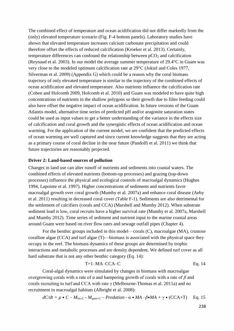
238
The combined effect of temperature and ocean acidification did not differ markedly from the
(only) elevated temperature scenario (Fig. F-4 bottom panels). Laboratory studies have
shown that elevated temperature increases calcium carbonate precipitation and could
therefore offset the effects of reduced calcification (Kroeker et al. 2013). Certainly,
temperature differences can confound the relationship between pCO2 and calcification
(Reynaud et al. 2003). In our model the average summer temperature of 29.4°C in Guam was
very close to the modeled optimum calcification rate at 29°C (Jokiel and Coles 1977,
Silverman et al. 2009) (Appendix G) which could be a reason why the coral biomass
trajectory of only elevated temperature is similar to the trajectory of the combined effects of
ocean acidification and elevated temperature. Also nutrients influence the calcification rate
(Cohen and Holcomb 2009, Holcomb et al. 2010) and Guam was modeled to have quite high
concentrations of nutrients in the shallow polygons so their growth due to filter feeding could
also have offset the negative impact of ocean acidification. In future versions of the Guam
Atlantis model, alternative time series of predicted pH and/or aragonite saturation states
could be used as input values to get a better understanding of the variance in the effects size
of calcification and coral growth and the synergistic effects of ocean acidification and ocean
warming. For the application of the current model, we are confident that the predicted effects
of ocean warming are well captured and since current knowledge suggests that they are acting
as a primary course of coral decline in the near future (Pandolfi et al. 2011) we think that
future trajectories are reasonably projected.
Driver 2: Land-based sources of pollution
Changes in land use can alter runoff of nutrients and sediments into coastal waters. The
combined effects of elevated nutrients (bottom-up processes) and grazing (top-down
processes) influence the physical and ecological controls of macroalgal dynamics (Hughes
1994, Lapointe et al. 1997). Higher concentrations of sediments and nutrients favor
macroalgal growth over coral growth (Mumby et al. 2007a) and enhance coral disease (Aeby
et al. 2011) resulting in decreased coral cover (Table F-1). Sediments are also detrimental for
the settlement of calcifiers (corals and CCA) (Marshell and Mumby 2012). When substrate
sediment load is low, coral recruits have a higher survival rate (Mumby et al. 2007a, Marshell
and Mumby 2012). Time series of sediment and nutrient input to the marine coastal areas
around Guam were based on river flow rates and sewage outfall pipes (Chapter 4).
For the benthic groups included in this model—corals (C), macroalgae (MA), crustose
coralline algae (CCA) and turf algae (T)—biomass is associated with the physical space they
occupy in the reef. The biomass dynamics of these groups are determined by trophic
interactions and metabolic processes and are density dependent. We defined turf cover as all
hard substrate that is not any other benthic category (Eq. 14):
T=1–MA–CCA–C Eq. 14
Coral-algal dynamics were simulated by changes in biomass with macroalgae
overgrowing corals with a rate of α and hampering growth of corals with a rate of β and
corals recruiting to turf and CCA with rate γ (Melbourne-Thomas et al. 2011a) and no
recruitment in macroalgal habitats (Albright et al. 2008):
dC/dt = µ • C – Mlin-C - Mquar-C – Predation - α • MA –β•MA + γ • (CCA+T) Eq. 15

239
dMA/dt = µ • MA – Mlin-MA - Mquar-MA – Predation + α • MA + β • MA Eq. 16
where µ is the growth rate, C is the biomass of corals, MA is the biomass of macroalgae,
CCA the biomass of crustose coralline algae, T the biomass of turf algae and Mlin and Mquar
are the linear and quadratic species-specific mortality rates. Furthermore, growth of primary
producers is dependent on light, space and nutrient limitation (full description of these
dynamics is detailed in (Fulton et al. 2004b)). We allowed for vertical growth, for example,
on the base of branching corals, under or at the sides of overhangs and boulders, by setting
the total benthic space available to 135% of planar area.
Coral growth can be further hampered by sediment. High sediment concentration in
the water column not only limits the light available for photosynthesis (captured in Atlantis
under light limitation), when sediment settles on the reef, corals have to divert some energy
to producing mucus to slough off those sediments. This energy is then not available for
growth. Using the empirical relationship derived from a study of sediment concentration and
change in coral abundance conducted in Guam (derived from Equation 1 in (Wolanski et al.
2004)) we included a function to capture this ‘smothering effect’:
S = Sa • ln(sed_level) + Sb Eq. 17
where S is the smothering effect, Sa the smothering coefficient and Sb the smothering
constant. The sed_level is the concentration of sediments in the water column and changes
over time mostly depending on riverine runoff.
We simulated two scenarios: (1) with estimated time series of river and sewage
outflow that contained sediments and nutrients (Weijerman et al. 2014b), and (2) no inputs.
Parameter estimates are given in Appendix G.
Land-based sources of pollution: Sedimentation and nutrient elevation effects on
benthic composition and target fish biomass
Point source and non-point source pollution and accompanying elevated nutrient and
sediment input into nearshore waters led to a rapid increase in phytoplankton and suspended
solids followed by an increase in macroalgae and CCA and a decrease massive corals (Fig. F-
5).
Increased sediment led to reductions in coral growth rates compared to the control
scenario (Fig. F-5). Consistent with nutrient enrichment experiments (Smith et al. 2001, Brian
et al. 2004) we had expected algal biomass to positively respond to nutrient input and that to
lead to reductions in coral cover, the effects of which were shown by our model (Fig. F-5).
The effect of sediments on the growth rate of corals and the competition between corals and
algae are modeled using the same parameters, since massive corals have a lower growth rate,
the effect is larger on massive corals.
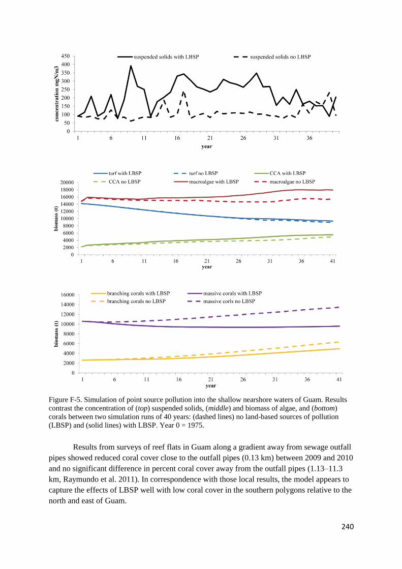
240
Figure F-5. Simulation of point source pollution into the shallow nearshore waters of Guam. Results
contrast the concentration of (top) suspended solids, (middle) and biomass of algae, and (bottom)
corals between two simulation runs of 40 years: (dashed lines) no land-based sources of pollution
(LBSP) and (solid lines) with LBSP. Year 0 = 1975.
Results from surveys of reef flats in Guam along a gradient away from sewage outfall
pipes showed reduced coral cover close to the outfall pipes (0.13 km) between 2009 and 2010
and no significant difference in percent coral cover away from the outfall pipes (1.13–11.3
km, Raymundo et al. 2011). In correspondence with those local results, the model appears to
capture the effects of LBSP well with low coral cover in the southern polygons relative to the
north and east of Guam.

241
Driver 3: Fishing activity
Parrotfish, grouped in large excavators and scrapers, fulfil an important ecological role by
opening up substrate for coral recruitment (Table F-1). The feedback loop between corals,
algae and grazers is possibly the most examined reef dynamic with minimal models,
exploring the existence and thresholds of stable states (Hughes 1994, Mumby 2006). Cover
of macroalgae on reefs is linearly negatively related to the biomass of herbivorous fishes
(Mumby 2006, Bellwood et al. 2011). However, studies in the Caribbean have shown that
herbivorous fishes can only maintain a maximum of 30%–40% of a reef structure in a
cropped state (Williams et al. 2001). Large parrotfishes are more effective grazers than small
ones (Ong and Holland 2010), for example, 75 small (< 15 cm) parrotfishes maintain the
same area of substrate in grazed states as one single individual of 35 cm (Lokrantz et al.
2008). In locations with high fishing pressure, large parrotfish are removed and, although
small parrotfishes will tend to increase in abundance due to predator release (Bellwood et al.
2011), the net effect of fishing pressure leads to reductions in grazing pressure potentially
leading to phase shifts.
Corals have a positive effect on fish abundance by providing shelter (McClanahan
1995, Wilson et al. 2008, Blackwood et al. 2011, Kerry and Bellwood 2012, Ainsworth and
Mumby 2014). Several studies have also demonstrated a positive relationship between coral
complexity and fish diversity (Friedlander and Parrish 1998, Jones et al. 2004, Paddack et al.
2009), especially for corallivores and planktivores (Graham et al. 2006). This positive
feedback appears to be driven by the increased survival of fish recruits and other small-
bodied fishes (Jones et al. 2004, Graham et al. 2006, Coker et al. 2013, DeMartini et al. 2013,
Rogers et al. 2014). Coral reef complexity is partly dependent on the topography of the reef
substrate itself (e.g., boulders provide complexity) and partly by coral growth (e.g., large
branching corals provide more shelter than small coral colonies). Benthic complexity values
ranging between 1 (flat) and 5 (high structural complexity) were taken from CRED survey
data and serve as a baseline. We then assume that changes in complexity reflect net coral
growth (i.e., the balance between accretion and erosion). We used the topographical
complexity model developed by Bozec et al. (2014) to calculate rugosity.
R = rug_constant • SI Eq. 18
where R = rugosity, rug_constant is the ratio of the vertical contour of a colony and the
surface-to-area ratio of a colony, SI is the deformation of the reef surface and is calculated as
the surface area of the reef (depending on height and diameter of coral colonies) divided by
the planimetric area of the reef which depends on the maximum diameter and coral cover
(Bozec et al. 2014).
Rugosity in turn affects the availability of prey to predators, according to the inferred
relation of the habitat scalar at time i based on (Graham et al. 2006, DeMartini et al. 2013):
hab_scalari = hab_scalar • (Rcoefft • ln(R) + Rconst) Eq. 19
In other words, rugosity affects the availability of prey fish to predators according to
the inverse of the habitat scalar relationship with a maximum capacity set at 4 and a scalar
coefficient depending on the species (varying between 0.6 for small species to 8.0 for
unaffected species). For parameter estimates see Appendix G.

242
To determine the adapted model’s capability to simulate the effects of the coral-algae-
grazer relationships with the added code, we simulated two scenarios: (1) intensive fishing on
herbivores (fishing mortality (F) of 0.8 per year), and (2) no fishing of herbivores. In both
scenarios we kept fishing on other groups low (F=0.05 per year). Similarly for the
relationship between complexity and fish biomass, we ran two 30-year simulations, one with
this relationship included and one without, assuming a low fixed fishing mortality of 0.05 for
all groups.
Effects of fishing of herbivores on corals-algae-grazers dynamics
The strong link between herbivorous fishes and the benthic community composition (high
herbivore biomass resulted in low macroalgal cover and high coral and CCA cover) is clearly
demonstrated in the scenarios with high (F=0.8) and no (F=0) fishing of herbivorous fishes
while keeping fishing on all other targeted groups to F = 0.05. Compared to no fishing of
herbivores (F=0), when herbivore fishing mortality was set to 0.8, biomass of turf and
macroalgae is 6% higher, and biomass of calcifiers is 7% lower at the end of a 30-year
simulation.
Scenarios with and without refuge effects from structural complexity showed the
importance of incorporating the effects of complexity into coral reef ecosystem models. Fish
biomass of most prey groups was enhanced by the three-dimensional complexity (Fig. F-6).
Planktivores in particular were dependent on refuge associated with structural complexity, as
their biomass was 6.6 times more in models with the complexity-refuge relationship enabled.
In contrast, predatory fish groups had a 0.1–0.5 times lower biomass when habitat refugia
relationships were included in models (Fig. F-6). Modeled increase in biomass of prey fish
with increased structural complexity was in correspondence with empirical relationships from
Guam (Appendix K).
Figure F-6. Ratio of biomass with refuge enabled versus no refuge enabled for each functional
vertebrate group and corals at the end of 40 year simulation run. Ratios are represented as logarithmic
values of the actual ratio.
Simulations demonstrated strong links between herbivorous fish biomass and the
benthic community, with herbivore biomass associated with low macroalgal cover and high

243
cover of coral and CCA, as has been shown on reef in American Samoa (Heenan and
Williams 2013), the Caribbean (Mumby et al. 2007a), the Great Barrier Reef (Wismer et al.
2009), Fiji (Rasher et al. 2012), but also in spatial surveys conducted around Guam (Williams
et al. 2012).
Additionally, model outcomes show the importance of reef structure as refuge for fish
species, by making them less vulnerable to predators. We parameterized this part of the
model based on the study of Bozec et al. (2014), but those relationships could potentially be
improved with site-specific data. Also the parameters used for erosion caused by fish, urchins
and boring sponges that affect the reef’s structural complexity should be updated with data
from Guam when such data becomes available to improve the model.
Sensitivity and skill assessments
We performed sensitivity assessments on primary productivity (growth rate of primary
producers), the structural complexity input parameters (diameter of corals), and the parameter
for direct coral-algal competition (the β in equation 15). From the literature we derived
plausible values for these parameters (Appendix G) and ran the model with the minimum and
maximum estimates to get boundaries for plausible trajectories. We then visually inspected
the derived cone of uncertainty (i.e., range of trajectories) to see which of the groups are
sensitive to the parameters and if the trajectory of the control run fitted into this cone.
To assess the model skill, we compared 2011 projected biomass of each fish group
against the observed biomass from CRED fish surveys conducted in 2011 using the root
mean squared error (RMSE) according to:
𝑅𝑀𝑆𝐸 = √∑ (𝑃𝑖−𝑂𝑖)2𝑛
𝑖=1
𝑛 Eq. 20
where n = the number of observations (fish groups), Oi = the ith of n observations, Pi = the ith
of n projections, and O and P are the observation and projected annual averages, respectively
(Stow et al. 2009).
Out of the three sets of parameters analyzed with a sensitivity assessment, only the
growth rates of plankton showed substantial variation in outcomes of selected fish groups and
coral biomass (Appendix J). For the rugosity (or structural complexity) sensitivity (the
parameter inputs being the mean diameter for branching and massive coral colonies) the
outcomes varied a little (mostly for the rugosity; Fig J-2), and target fish groups and corals
were not sensitive to the parameter for coral-algal competition (Fig. J-3). When varying the
growth rates of phytoplankton, most vertebrate groups showed a narrow cone of uncertainty,
i.e., they are not sensitive to changes in these growth rates (Fig. J-1). Our control run
estimates were in the middle of the cone for 10 out of the 13 target fish species, giving more
confidence in the model results with regard to fish groups. However, coral cover and, hence,
rugosity are much more sensitive to these changes making it important to get good estimates
of the growth rates of these groups. Since we did not run the control scenario with the mean
of the primary producers’ growth rates, but rather the maximum of large phytoplankton and
lower than the average for small phytoplankton, the projected biomass (red line in Fig. J-1)
does not necessarily need to be in the middle of the cone. Future versions of Guam Atlantis

244
should look more into the effect of the predicted variation in coral biomass as a response to
the changes in growth rates of primary producers to help explain the high biomass trajectory
in corals (top or above the cone) and the odd shape of the relationship between planktivores
and plankton (where one could expect a linear relation).
Formal skill assessment of the Guam Atlantis model is impossible due to the lack of
time-series of observed data. Instead we compared the observed biomass estimates from 2011
visual surveys conducted by CRED with the projected biomass in 2015 after simulating the
status quo scenario for 30 years. Skill assessment results show that for fish groups with lower
abundance (less than 50 t) model predictions at the end of a 30-year simulation corresponded
reasonably well (RMSE = 14) with observations from visual surveys. For the more abundant
species, model predictions were consistently above the observed estimates resulting in a very
high value of RMSE (198) suggesting that the model has a bias (Fig. F-7). The largest
discrepancy was for scrapers (parrotfish) and grazers (triggerfish, gregory, damselfish), and
to a lesser extend for invertivores, planktivores and target grazers (surgeon fish). This result
implies that either those fish groups are too productive in our model or that we
underestimated the mortality. Since fish productivity responded reasonably to increased
fishing mortality (Fig. H-4), it seems more likely that we underestimated fishing mortality,
particularly because the fishery data did not capture all gear types equally well (K. Lowe,
NOAA-PIFSC, pers. comm.). Fishing mortality is based on voluntary creel surveys and we
did not take into account the boat-based fishery, for a future version of this Guam Atlantis
model better fishery estimates are necessary to account for this difference.
Figure F-7. Observed versus projected biomass of fish groups in 2011. Observations are from visual
surveys conducted by NOAA Coral Reef Ecosystem Division in 2011, projected values are the mean
of the last five years at the end of a 30-year run representing 2010–2015.
1:1

245
Conclusion
The adapted Guam Atlantis model met the three main criteria for Atlantis model development
and is stable with plausible biomass trajectories. The paucity of time series of observational
data prevented a formal skill assessment, but the model was able to reproduce biomass
trajectories after disturbances (e.g., effects of climate change and sediment and nutrient
inputs) that corresponded with expectations based on published relationships giving us
confidence in the model validity. Additionally, the coral-algae-grazer dynamics are well
simulated by the model with model outcomes comparable to expectations in response to low
herbivorous biomass as well as the relationship between reef’s structural complexity and its
ability to provide refuge for prey fishes. Despite room for improvement (e.g., on historical
fisheries catches and alternative predictions of pH and aragonite saturation) the model
simulates the complex dynamics within a coral reef ecosystem well. However, in the future
uncertainty in model outcome would be better captured by comparing model predictions
across a range of parameterizations of the model.

246
Appendix G
This supplement provides additional information for chapter 6: “Applying the Atlantis model
framework to coral reef ecosystems”. It details the coral code related parameters.
Parameter value mini mum
maxi mum
unit source
Growth related:
Autotrophic feeding
light threshold for feeding 700 W/m2 assuming 15% of noon sunlight
corals feeding during day 20 %
translocation of nutrients to
host 90 % Gustafsson 2013
Sediment smothering effects
Ksmother coefftient; 0.054 nd Wolanski et al. 2003a
Ksmother_constant; 0.4622 nd Wolanski et al. 2003a
Algal-coral competition
max growth rate massive
corals 0.0003 0.00011 0.019 d
-1 0.003 (Mumby); 0.003 (Weijerman
et al. 2013); 0.0004-0.0194 (Ruiz
Sebastián and McClanahan 2013);
0.00011-0.0055 (Melbourne-
Thomas et al. 2011a) max growth rate branching
corals 0.0003 0.00011 0.059 d
-1
max growth rate turf 0.075 0.027 0.4 d-1 0.029 (Klumpp and McKinnon
1992); 0.027 (Miller et al. 2009);
0.04 (Ruiz Sebastián and
McClanahan 2013); 0.05-0.4
(Melbourne-Thomas et al. 2011a) max growth rate macroalgae 0.018 0.014 0.4 d
-1 0.018 (Klumpp and McKinnon
1992); 0.06 (Dailer et al. 2012)
(Kappaphycus); 0.014 (Ruiz
Sebastián and McClanahan 2013);
0.05-0.4 (Melbourne-Thomas et al.
2011a) max growth rate CCA 0.01 0.01 0.026 d
-1 0.010 (Klumpp and McKinnon
1992, Weijerman and Brown
2013); 0.026 (Ruiz Sebastián and
McClanahan 2013) max growth rate small
phytoplankton 0.41 0.41 3.2 d
-1 0.41 (Weijerman et al. 2013); 3.2
(Wang et al. 2008) max growth rate large
phytoplankton 4.1 0.41 6.4 d
-1 0.41 (Weijerman et al. 2013); 6.4
(Wang et al. 2008) turf-coral overgrow (rate of
growth suppression) 0 McCook et al. 2001

247
Parameter value mini mum
maxi mum
unit source
macroalgae-coral overgrow
(rate of growth suppression) 0.0010 0.00014 0.0011 d
-1 McCook et al. 2001, Lirman 2003,
Mumby and Dytham 2005,
Melbourne-Thomas et al. 2011a CCA-coral overgrow (rate of
growth suppression) 0 (McCook 2001)
turf-coral facilitation (%
facilitation of coral
recruitment)
5 5 15 % McCook et al. 2001, Melbourne-
Thomas et al. 2011a
macroalgae-coral competition
(% growth inhibition) 80 40 90 % McCook et al. 2001, Melbourne-
Thomas et al. 2011a CCA-coral facilitation (%
facilitation of coral
recruitment)
5 5 15 % McCook et al. 2001, Melbourne-
Thomas et al. 2011a
half saturation constant for
growth on DIN for massive
corals
50 5.6 28 mgN/
m3
0.23-0.8 µM NO3 (Domotor and
D'Elia 1984); 5-22µM NO3 (D'Elia
et al. 1983) half saturation constant for
growth on DIN for branching
corals
50 5.6 28 mgN/
m3
5.6-28 (0.4-2.0 µM); NO3 0.23-0.8
µM (Domotor and D'Elia 1984); 5-
22uM (D'Elia et al. 1983) half saturation constant for
growth on DIN for turf algae 6 mgN/
m3
half saturation constant for
growth on DIN for
macroalgae
6 1.4 11.2 mgN/
m3
0.1-0.8 mmol/m3 (Lapointe 1997)
half saturation constant for
growth on DIN for CCA 6 mgN/
m3
half saturation constant for
growth on DIN for small
phytoplankton
0.35 0.0084 1.4 mgN/
m3
0.025 mmol/m3 (Huisman et al.
2006); 0.6 nmol/m3 (Wang et al.
2008); 0.1 mmol/m3 (Lapointe
1997) half saturation constant for
growth on DIN for large
phytoplankton
0.35 0.0028 1.4 mgN/
m3
0.025 mmol/m3 (Huisman et al.
2006); 0.2 nmol/m3 at (Wang et al.
2008); 0.1 mmol/m3 (Lapointe
1997) light saturation branching
corals 35 11 67 W/m
2 50-300 µE/m2/s (Kleypas 1997)
light saturation massive
corals 35 11 67 W/m
2 50-300 µE/m2/s (Kleypas 1997)
light saturation turf 5 W/m2
light saturation macroalgae 5 W/m2 Skagerrak & Baltic Sea ~ 100 µmol
photons/m2/s= 0.135 W/m
2
light saturation CCA 5 W/m2
light saturation small
phytoplankton 20 W/m
2 Huisman et al. 2006
light saturation large
phytoplankton 20 W/m
2 Huisman et al. 2006
Rugosity related: rugosity based habitat
dependency coefficient 1.4613 nd Shape of relationship inferred from
Friedlander and Parrish 1998,

248
Parameter value mini mum
maxi mum
unit source
rugosity based habitat
dependency constant 0.0475 nd Graham et al. 2006, DeMartini et
al. 2013 rugosity based habitat
dependency cap 4 nd
rugosity based habitat
dependency scalar 8 nd
rugosity constant 1.3 nd adapted from Bozec et al. 2014
massive corals colony height
parameter 0.715 cm Bozec et al. 2014
branching corals colony
height parameter 0.81 cm average of slopes from Porites sp.
(Bozec et al. 2014) branching corals max. colony
diameter 60 0-5 >300 cm mean 26 cm L. Raymundo,
unpublished data, 17 cm CRED
data massive corals max. colony
diameter 30 0-5 >300 cm mean 14 cm L. Raymundo,
unpublished data, 15 cm CRED
data
Ocean change related Aragonite saturation - CO3 calculation
Karag_A 0.9485 nd Zeebe and Wolf-Gladrow 2009;
Values for coefficients from proxy
fitting exercise - from data given in
Bjerrum plot
Karag_B 8.20416 nd
Karag_C 2.3641 nd
Karag_D 8 nd
Karag_pH; time
series
pCO2
nd IPCC AR5 RC8.5; for control
simulation: pCO2 =380 (~1985)
Kca_const; 0.0103 Berner 1965, Edmond and Gieskes
1970, Kleypas et al. 2006 K_Ks; 6 10
-9 nd Kleypas et al. 2006
Calcification related parameters
Reference baseline
calcification rate 15.03 12.03 17.03 ppm 380 ppm (Silverman et al. 2009,
Anthony et al. 2011a) needed to
lower to get realistic rates of
calcification calcification T constant 9.7 9.03 10.37 nd Silverman et al. 2009, Anthony et
al. 2011a calcification T coefficient 18.83 12.98 24.68 nd Silverman et al. 2009, Anthony et
al. 2011a calcification optimum
temperature 29 °C close to summer ambient
temperature (Jokiel and Coles
1977); summer solstice temp.
(Silverman et al. 2009) calcification Lambda 0.42 0.33 0.51 nd Silverman et al. 2009, Anthony et
al. 2011a light threshold for
autotrophic feeding 700 W/m
2 assumption 85% of noon irradiance

249
Parameter value mini mum
maxi mum
unit source
proportion feeding during
light 20 % assuming mostly feeding at night
host remineralization 90 % Gustafsson 2013
Growth/fecundity relationship with pH
CCA coeff. & const -7.0, 1.0 nd Langdon 2002, Kroeker et al. 2010
large phytoplankton coeff. &
const 1.4,
1.1705 nd Hendriks et al. 2010, Harvey et al.
2013 small phytoplankton coeff. &
const 3.7, 1.0 nd Hendriks et al. 2010, Harvey et al.
2013 macroalgae coeff. & const 1.6, 1.1 nd Hendriks et al. 2010, Harvey et al.
2013 zooplankton coeff. & const 5.0, 1.7 nd Kurihara and Ishimatsu 2008,
Hendriks et al. 2010, Wittmann and
Pörtner 2013 benthic grazers (urchins)
coeff. & const -3.0, 0.5 nd Kurihara and Ishimatsu 2008,
Hendriks et al. 2010, Wittmann and
Pörtner 2013 benthic filter feeders
(bivalves) coeff. & const -7.0, 1.0 nd Wittmann and Pörtner 2013
Bleaching parameters
bleaching mortality massive
corals 22.5 3.14 41.87 % Jokiel and Coles 1990,
McClanahan , Donner et al. 2005,
McClanahan et al. 2007 bleaching mortality
branching corals 42 19.7 100 %
bleaching rate massive corals 25 9.8 40.2 %
bleaching rate branching
corals 24.2 6.9 41.5 %
bleaching recovery rate
massive corals 0.0027 d
-1 Lombardi et al. 2000
bleaching recovery rate
branching corals 0.0822 d
-1 Kvitt et al. 2011 (0.2 degree
/decade) bleaching temperature corals 30.4 °C 1 degrees above summer max
ambient, NOAA Coral Reef Watch proportion of zooxanthellae
in coral tissue 30 5 30 % 15% (Odum and Odum 1955);
<5% (Thornhill et al. 2011);
30% (Gustafsson 2013) degree heating weeks (DHW)
threshold massive corals 4 DHW Donner et al. 2005, McClanahan et
al. 2007 degree heating weeks (DHW)
threshold branching corals 3 DHW Donner et al. 2005, McClanahan et
al. 2007

250
Appendix H
This supplement provides additional information for chapter 6: “Applying the Atlantis model
framework to coral reef ecosystems”. It shows example outputs from control simulations (i.e.,
a run with no external disturbances) of trajectories in fish biomass, invertebrate biomass,
weight-at-age and numbers-at-age. The last figure (H-4) shows catch and biomass
equilibrium plots.
Figure H-1. Biomass trajectories of some fish, invertebrate, planktonic, and benthic functional groups
of a scenario when no external disturbances were simulated. The green dashed line reflects the
biomass in marine preserves in Guam (CRED surveys conducted in 2011). The blue dashed line
represents the biomass calculated from surveys around the unpopulated Northern Mariana Islands.

251
Figure H-2. The trajectory of the ratio of weight-at-age to initial weight-at-age of vertebrate functional
groups of a scenario when no external disturbances were simulated. The rainbow colors represent the
ten age classes with red being the youngest and violet being the oldest age class.

252
Figure H-3. The trajectory of abundance-at-age of vertebrate functional groups of a scenario when no
external disturbances were simulated. The rainbow colors represent the ten age classes with red being
the youngest and violet being the oldest age class.

253
Figure H-4. Catch and biomass equilibrium plots for functional groups: catch (blue dashed line – right
vertical axis) and biomass (black line – left vertical axis) against fishing mortality (F=0, 0.05, 0.08,
0.10, 0.20, 0.30, 0.50, 0.80). X-axis is fishing mortality per year, left y-axis is the biomass in tons, and
right y-axis is the landings in tons. Both biomass and catches are shown at the end of a 30-year
simulation. Natural mortality for target invertivores = 0.49/y; humphead wrasse = 0.15/y; target
browsers = 0.32/y; target grazers = 0.19/y; scrapers = 0.53/y; excavators = 0.41/y; bunphead
parrotfish = 0.14/y; target benthic piscivores = 0.29/y; mid-water piscivores = 0.51/y; roving
piscivores = 0.16/y; rays = 0.17/y; sharks = 0.21/y.

254
Figure H-5. Annual fish catches from a few functional groups. Blue squares are catches from the
model output (forced with historical catches as far as possible given modelled ecosystem structure)
and red diamonds are reported catches from creel survey data (Guam Division of Aquatic and
Wildlife Resources).FPL=planktivores; FDE=detritivores; FHG=grazers; THG=target grazers;
TIV=target invertivores; and FPR=roving piscivores.

255
Appendix I
This supplement provides additional information for chapter 6: “Applying the Atlantis model
framework to coral reef ecosystems”. Model predictions of biomass trajectories of the
functional groups were compared to reconstructed time series from fishery-dependent
(CPUE) and fishery-independent (visual survey) data of targeted fish species. There was a
substantial discrepancy for the functional groups with low abundance data, such as the
humphead wrasse, bumphead parrotfish, and sharks, but also for many of fish species
targeted by spear fisherman (e.g., parrotfishes). Reported catch data (DAWR) showed a
decline in catches in the last decade, this decline in landings (and effort) is reflected in an
increase in fish biomass since 2005 (Fig. I-1 left bottom panel) which was not seen in reality
(Brainard et al. 2012).
Figure I-1. Results from simulating historical catches with (left panels) biomass trajectory and (right
panels) the catches (in blue) and estimated actual catches (in red; data from DAWR) of (top)
humphead wrasse (HHW), (middle) targeted invertivores (e.g.,snappers, goatfish, emperor; TIV) and
(bottom) large-bodied parrotfish (FHE)

256
When we assumed fish catches since 2005 stayed similar to fish catches between
2000 and 2004 for those species heavily targeted by spearfisherman i.e., for parrotfishes
(FHE, FHS), goat fishes (TIV), humphead wrasse (HHW), and unicorn fishes (THB), the
trend of the predicted biomass corresponded better with the estimated biomass based on the
reconstructed time series (Fig. I-2).
Figure I-2. Results from simulating historical catches with spearfish catches of the last decade of
parrotfish at same levels as the average of 1999-2004. (left panel) Biomass trajectory (in diamonds)
compared to reconstructed time series (in triangles) and (right panel) the catches (in blue) and
estimated actual catches (in red) of (top) large-bodied parrotfish (FHE).

257
Appendix J
This supplement provides additional information for chapter 6: “Applying the Atlantis model
framework to coral reef ecosystems”. It shows the results of three sensitivity analyses.
Figure J-1. Sensitivity of selected functional groups to growth rates of large and small phytoplankton.
The shaded area represents the area between the minimum and maximum values used for these
parameters (see Appendix G for parameter values). The red line is the trajectory of the control run.

258
Figure J-2. Sensitivity of selected functional groups to rugosity estimations. The shaded area
represents the area between the minimum and maximum values used for the mean coral diameter
parameters (see Appendix G for parameter values). The red line is the trajectory of the control run.

259
Figure J-3. Sensitivity of selected functional groups to relationship between coral and macroalgae.
The shaded area represents the area between the minimum and maximum values used for this
parameter (see Appendix G for parameter values). The red line is the trajectory of the control run.

260
Appendix K
This supplement provides additional information for chapter 6: “Applying the Atlantis model
framework to coral reef ecosystems”. From reef-fish surveys around Guam conducted by
CRED, the empirical relationship between structural complexity and fish biomass is apparent
from all the upward trend lines in Figure K-1.
Figure K-1. Relationships between the structural complexity and the reef-fish biomass of six
functional groups around Guam. Blue line is linear regression line with shaded area representing 95%
confidence region. Data from visual surveys conducted by NOAA-PIFSC-CRED in 2011.
261
Appendix L
This supplement provides additional information for chapter 8: “Towards an ecosystem-
based approach of Guam’s coral reefs: the human dimension”. It shows a list of
participating organizations in the workshop and meetings conducted in Guam in 2011 and
2014
Organization
NOAA Fisheries Pacific Islands Regional Office (PIRO)
NOAA Pacific Islands Fisheries Science Center (PIFSC)
NOAA Coral Reef Conservation Program (CRCP)
NOAA-PIFSC – Coral Reef Ecosystem Division
JIMAR - University of Hawai’i
POC Coral Reef Conservation, Western Pacific Fishery Management Council, Director of
Dept. of Chamorro Affairs
Guam Coastal Management Program (GCMP)
Guam Department of Agriculture
University of Guam Marine Laboratory
Humatåk Community Foundation
Guam Preservation Trust
Naval Facility Andersen Air Force Base (AAFB)
USDA Natural Resource Conservation Service
War in the Pacific National Park (NPS)
Guam Environmental Protection Agency

262
Appendix M
This supplement provides additional information for chapter 8: “Towards an ecosystem-based approach of
Guam’s coral reefs: the human dimension”. It describes the nodes in the dive tourism behavior model. Starred
(*) nodes connect directly to the ecological model.
Node Description of node
Wreck diving The presence or absence of a wreck at a dive site. Guam has several historic wrecks in Apra
Harbor which are popular dive locations
Quality of dive
experience The combination of ecological and situational variables that influence overall satisfaction
Previous dive
experience The total number of dives an individual has previously completed
Cost of dive charter The price paid to participate in a dive
Tourist visitation # The number of tourists visiting the island
Tourist origin Tourists from different countries do not all have the same preferences
Age group The age of an individual (in years)
Price of
accommodation Price paid for hotel accommodations can vary throughout the year
Charismatic species* The presence or absence of charismatic species, such as, bumpead parrotfish, Napoleon wrasse,
sharks, turtles
Coral cover* The average of coral cover in the entire model domain
Species abundance*
Species abundance is the standing stock biomass of the main species that comprise the fishery
target groups (e.g., jacks, parrotfish, groupers, surgeonfish, goatfish, invertebrates) and non-target
groups. The standing stock biomass changes over time due to habitat degradation and extraction.
Clarity of the water Sediments and algal blooms can reduce the clarity of the water, and thus visibility.
Tourist season Peak: January to May; Off season: July to November; June and December are shoulder months.
Flight availability The number of flights arriving in Guam per month
Access to diving
locations
Access to coastline areas and potential dive sites is restricted by the natural features of the
coastline in Guam, ocean and weather conditions, and military/security access controls.
Watershed condition
A description of the watershed as degraded or not. Degraded watersheds are assumed to have the
same run off of sediments and nutrients as present conditions. When watersheds are restored, we
assume no additional sediment and nutrient inputs.
Marine preserves
Guam has 5 marine preserves: Tumon Bay MP, Piti Bomb Holes MP, Pati Point MP, Sasa Bay
MP, and Achang MP. There are specific rules regulating fishing and other activities for each
one. They cover approximately 16.3% of Guam's coral reef habitat from 0 to 30-m depth.
Ocean and weather
conditions
Ocean and weather conditions that may change on a daily or seasonal basis, such as wind speed
and direction, wave height, tides, and visibility; Waters in some areas around the island are too
rough for diving during much of the year.
Coastal features Access to Guam’s coastline areas and potential dive sites is restricted by natural features
Access areas closed
by military
Areas of the shoreline, territorial waters (out to 3 nm), and federal waters (3 - 200 nm) that are
closed to fishing activities by the U.S. military and/or territorial and federal security agencies
(e.g., the U.S. Department of Homeland Security).
Enforcement of
marine preserves The effectiveness of enforcement of rules regulating fishing and boating activities.

263
Appendix N
This supplement provides additional information for chapter 8: “Towards an ecosystem-based approach of Guam’s coral reefs: the human dimension”. It
describes connection between nodes of dive tourism behavior model
Variable A Variable B Connection between variables Reference
Enforcement Marine
preserves
The effectiveness of enforcement can determine if dive charters respect
the rules regulating fishing and other activities within marine preserves. Expert opinion
Marine
preserves
Species
abundance
The establishment (and enforcement) of marine preserves may influence
the overall abundance of species and in particular in species that complete
their life cycle within the marine preserve boundaries. Moreover, spillover
effects may lead to a greater biomass or fish abundance of species just
outside of the marine preserve boundaries.
Tupper 2007
Marine
preserves
Charismatic
species
The establishment (and enforcement) of marine preserves influences the
overall abundance of charismatic species and in particular in species that
complete their life cycle within the marine preserve boundaries.
Tupper 2007
Marine
preserves Coral cover
There is little evidence that marine preserves increase coral cover, as coral
cover increase is related to herbivore biomass. However, herbivore
biomass increases within marine preserves.
Gilmour et al. 2013
Watershed
conditions Turbidity
Different types of land use will have a different effect on runoff and thus
ocean turbidity. Turbidity created by different land uses can be a problem
in some areas of Guam. If the watershed is in good condition this will
decrease runoff and thus turbidity.
Burdick et al. 2008
Oceans and
weather
conditions
Turbidity Windy and stormy conditions can increase ocean turbidity. Wolanski et al. 2003a
Oceans and
weather
conditions
Access to diving
locations
Changes in ocean and weather conditions occur on a daily basis. Some
weather conditions will not allow dive activities to take place. In addition,
near shore waters on the east side of the island are too rough for diving.
Expert opinion

264
Variable A Variable B Connection between variables Reference
Coastline
features
Access to diving
locations
Cliff lines make up a significant portion of the coastline and prevent
coastal access for dive charters, particularly on the east side. The most
popular dive destinations are on the west side of the island due to the
presence of fringing reefs and bays and are accessible for dive charter for
most of the year.
http://www.mdaguam.com/content/guam-beach-
dives
Areas closed by
military
Access to diving
locations
Military areas are off limits and no access can be gained for dive
charters. Further, construction in preparation for the military buildup has
also inhibited access to municipal boat ramps, limiting the number of boat
access points.
Expert opinion
Access to
diving locations
Cost of dive
charter
Decreased access to dive grounds from the shoreline can increase the
distance boats need to travel, in turn, increases fuel use. With higher fuel
prices are likely to be passed on to the customers.
Expert opinion
Tourist season Cost of dive
charter
In peak tourist season the cost of dive charters is higher as demand for
charters is relatively higher. Expert opinion
Tourist season Price of
accommodation In the peak tourist season the price of accommodation is higher. Expert opinion
Tourist season Flight
availability In peak seasons there are more flights available to bring tourists to Guam. Expert opinion
Price of
accommodation
Tourist visitation
numbers
If prices of accommodation are comparatively high this means that
tourism visitation is likely to be negatively affected. Expert opinion
Flight
availability
Tourist visitation
numbers
If more flights are available this is likely to increase the number of tourist
visiting Guam. Expert opinion
Flight
availability
Tourist country
of origin
There are more flights to Guam from some countries thus influencing the
country of origin of the tourists. Expert opinion
Wreck diving Participation in
dive trips
There are a number of popular wreck dives with historical significance in
Apra Harbor, so the presence/absence of a wreck could also influence
participation in dive trips.
http://www.nps.gov/submerged/Parks/WAPA.ht
ml
Tourist
visitation #
Participation in
dive trips
With higher tourist number the demand for dive trips is also likely to
increase. Expert opinion
Cost of dive
charter
Participation in
dive trips
More expensive dive trip costs is likely to negatively affect participation
in dive trips. Rudd and Tupper 2002
Previous dive Participation in People with previous dive experience are more likely to participate in new Expert opinion

265
Variable A Variable B Connection between variables Reference
experience dive trips dive experiences and partake in dive trips on their holidays.
Age Previous dive
experience
Age group influences previous dive experience with older divers generally
having completed more dives. Grafeld et. al. (in prep)
Quality of the
dive experience
Participation in
dive trips
Positive dive experiences will mean that it is more likely that the tourist
will participate in a dive trip. Expert opinion
Size of dive
group
Quality of the
dive experience
Previous studies have included the size of the group on a dive charter as a
measure of the quality of the dive experience (with a higher WTP for
smaller groups).
Rudd and Tupper 2002, Schuhmann et al. 2013
Charismatic
species
Quality of the
dive experience
Charismatic species are important contributors to a dive experience. Some
divers will value the sighting of charismatic species most as part of the
dive trip.
$5.40 more/per ive to see more Napoleon
wrasse
(Grafeld et al. in prep)
Coral cover Quality of the
dive experience
The condition and extent of coral cover will increase the aesthetic quality
of the reef and thus increase the quality of the dive experience. Parsons and Thur 2008
Species
abundance
Quality of the
dive experience
The more species are visible and present on a dive – the more divers are
likely to enjoy the experience.
$6.45 more per dive for a change from low to
high fish biomass;
$6.23 more per dive for a change from low to
high fish species diversity
(Grafeld et al. in prep)
Turbidity Quality of the
dive experience
If turbidity is high- visibility is low and likely to decrease the quality of
the dive experience.
$10 on average (± $5) towards sediment
reduction projects
(Grafeld et al. in prep)
Tourist country
of origin
Tourist visitation
numbers
There are more tourists from some countries than others (i.e., Japanese
tourists make up the largest group).
https://www.fhb.com/en/assets/File/Marketing/F
HB_2013-14_GuamEconForecast.pdf

266
Appendix O
This supplement provides additional information for chapter 8: “Towards an ecosystem-based
approach of Guam’s coral reefs: the human dimension”. It describes the nodes in the fishery behavior
model. Starred (*) node connects to ecological model.
Node Description of node
Enforcement The effectiveness of enforcement of rules regulating fishing and boating activities.
Areas closed by
military/security
Areas of the shoreline, territorial waters (out to 3 nm), and federal waters (3–200 nm) that are
closed to fishing activities by the U.S. military and/or territorial and federal security agencies.
Ocean and weather
conditions
Ocean and weather conditions may change on a daily or seasonal basis, such as wind speed and
direction, wave height, tides, and visibility; waters in some areas around the island are too rough
for fishing from small boats during much of the year.
Coastline features Access to Guam’s coastline areas and nearshore fishing areas is restricted by the natural features.
Access to shoreline
and fishing grounds
Whether or not fishers can enter and/or utilize coastal and marine areas for fishing. Types of
areas include coastal access roads, beaches, boat ramps, docks/piers and marine areas.
Tourist season Peak: January to May; Off season: July to November; June and December are shoulder months.
Price of fish The price for which fish are bought and sold on Guam. This depends on several factors,
including seasonal availability of fish, time of year/tourist season, and outlet to which fish is
being sold (Guam Fishermen's Co-op versus restaurants versus other markets).
Fuel cost The cost of fuel. This is the main operating cost incurred in boat-based fishing on Guam.
Employment
opportunities
1) Whether or not fishers earn income from non-fishing employment, 2) Whether or not that
employment provides them with money beyond what is needed to meet regular expenses,
allowing them to have "free time" and extra income.
Age Age of fisher (in years)
Gender Gender of fisher
Fishing tradition Whether or not one comes from a "fishing family"; whether one's family members (especially
older family members) are fishers.
Ethnicity Ethnicity of fishers; people of some ethnicities are more likely to be engaged in fishing in Guam.
Species abundance Species abundance is the standing stock biomass of the main species that comprise the fishery
target groups (e.g., jacks, parrotfish, groupers, surgeonfish, goatfish, invertebrates) and
others. The standing stock biomass changes over time due to habitat degradation and extraction.
Participation in reef
fishing
Any activity that involves the collection of reef species. On Guam, this includes commercial
fishing and non-commercial fishing. Fishers often use multiple fishing gears and target multiple
marine species during a single fishing trip. Fish may be used for subsistence, given away or sold
depending on a variety of trip-based factors. When and where one fishes, which methods are
used, and which species are targeted depends on several factors, including the experience level of
fishers and access to resources required to fish (e.g., boat, gear, fuel).

267
Appendix P
This supplement provides additional information for chapter 8: “Towards an exosystem-based approach of Guam’s coral reefs: the human dimension”. It
describes connections between nodes in the fishery behavior model. Starred (*) node connects to ecological model.
Variable A Variable B Connection between variables Reference
Enforcement Management
scenarios
The effectiveness of enforcement can determine if fishers respect and observe the rules
regulating fishing activities.
Charles et al. 1999,
Sutinen and Kuperan
1999, Hatcher et al.
2000
Management
scenarios
Species
abundance
Alternative management scenarios will affect species abundance differently. For example,
the existence (and enforcement) of marine preserves may influence the overall abundance of
species, particularly for species that complete their life cycle within the marine preserve
boundaries. Size-based controls influence the overall abundance by limiting the fish allowed
to be landed to those of a specific size. With a build-up of larger (older) individuals, larval
quality and survivorship increases. Leaving the small, immature fish will increase the
spawning biomass.
(Berkeley et al. 2004,
Birkeland and Dayton
2005, Taylor et al. 2012,
Williams et al. 2012)
Management
scenarios
Access to
shoreline and
fishing grounds
Some management scenarios (such as the existence/expansion of MPs) may prevent fishers
from accessing certain shoreline and nearshore areas, sometimes restricting access to
common or traditional fishing grounds.
Expert opinion and
personal observation
Areas closed by
military/security
Access to
shoreline and
fishing grounds
Closed areas limit the ability of fishers to access fishing grounds. Further, construction, in
preparation for the military buildup, has also inhibited access to municipal boat ramps,
restricting boat access to nearshore fishing grounds. Fishers have to make longer boat trips
to get to their fishing locations.
Expert opinion and
personal observation
Ocean and
weather
conditions
Access to
shoreline and
fishing grounds
Changes in ocean and weather conditions occur on a daily and seasonal basis and contribute
to fishers' decisions regarding whether to go fishing and where they will fish. Some
nearshore waters on the east side of the island are too rough for fishing from small boats for
approximately 9 months of the year, on average.
Expert opinion

268
Variable A Variable B Connection between variables Reference
Coastline
features
Access to
shoreline and
fishing grounds
Coastline features determine the extent of coastal access for fishers. For example, cliff lines
make up a significant portion of the coastline and prevent access to adjacent fishing grounds.
Allen and Bartram 2008
Access to
shoreline and
fishing grounds
Fuel cost Decreased access to shoreline and fishing grounds can increase the distance boats need to
travel to preferred fishing grounds; this, in turn, increases fuel use. With higher fuel prices,
the cost to travel further distances increases. Fuel is the main operating cost incurred in
fishing on Guam. Increased fuel costs influence where and how often fishermen decide to
fish.
Hospital and Beavers
2012
Expert opinion
Access to
shoreline and
fishing grounds
Participation in
reef fishing
Access to fishing grounds can affect fishers’ decision to fish via expectations for: financial
profit, catching fish as food, and/or passing on fishing tradition. Access also affects decisions
regarding when and where to fish, which gear to use, and which species to target. Further,
restrictions to access may focus fishing in smaller areas, encouraging competition and local
depletion in remaining open areas.
Halpern et al. 2004,
Allen and Bartram 2008
Tourist season Price of fish Tourist season affects the price of fish because prices tend to be higher during high season
when the demand is high for certain species.
Expert opinion
Price of fish Participation in
reef fishing
The current price of fish may determine: 1) whether one decides to go fishing, 2) the fishing
method used (including location, gear used, and species targeted), and 3) what is done with
the catch once landed (kept, given away/shared, sold).
Expert opinion
Employment
opportunities
Participation in
reef fishing
Fishing activities can be affected by: 1) whether fishers earn income from non-fishing
employment, and 2) whether that employment provides them with money above and beyond
what is needed to meet regular expenses. Fishers who hold jobs that provide them with extra
income, and who have "free time," are able to buy and maintain a fishing boat and fishing
gear, and afford the expenses of fishing trips. The fish they catch may be used for household
consumption, given away, or sold for extra income to recoup fishing trip costs. Fishers who
do not earn sufficient income may have a greater incentive to fish to provide food for their
households.
Expert opinion

269
Variable A Variable B Connection between variables Reference
Fuel cost Participation in
reef fishing
Fuel is the main operating cost incurred in boat fishing on Guam. As fuel prices increase,
less of the fuel cost is recovered either when selling fish or when used as food. Above some
price for fuel, fishers may decide not to go out fishing because it is not worth the investment
in fuel. Therefore, increased fuel costs influence where and how often fishers decide to fish,
which gear to use, and which species to target.
Hospital and Beavers
2012
Age Participation in
reef fishing
In general, younger people are more likely to fish than older people, especially physically-
demanding activities such as spear fishing.
Expert opinion
Gender Participation in
reef fishing
Men are much more likely to fish than women. Expert opinion and
personal observation
Fishing tradition Participation in
reef fishing
Individuals are more likely to fish if they come from a "fishing family," and/or if other
members of their families are fishers.
Expert opinion
Ethnicity Participation in
reef fishing
Individuals are more likely to fish if their ethnicity has been historically engaged in fishing. Allen and Bartram 2008
Species
abundance*
Participation in
reef fishing
The overall abundance of marine species may determine: 1) whether one decides to go
fishing, 2) the fishing method used (including location, gear, species targeted), and 3) what is
done with the catch once landed (kept, given away/shared, sold).
Expert opinion

270
Summary
Widespread coral reef decline, including decline in reef fish populations upon which many
coastal human populations depend, have led to phase-shifts from the coral-dominated
systems, found desirable by humans, to algal-dominated systems that provide less ecosystem
services, and the loss of functionally important species. Marine resource managers are
challenged with providing strategies that can mitigate or prevent such phase shifts and losses
and promote the sustainable use of marine resources. Additionally, managers need to take
into account the impacts of these strategies on the socioeconomic conditions of the many
resource users. To respond to these challenges scientists, managers and policy makers have
advocated for an ecosystem-based approach instead of the traditional focus on individual
(economically important) species. Ecosystem-based management includes the various
dynamic processes that influence an ecosystem, such as hydrology, ecology,
biogeochemistry, and human activities.
The management strategy evaluation (MSE) tool commonly used in single species
stock assessments for evaluating socioeconomic and ecological tradeoffs of alternative
management strategies, has now become more widely applied in multi-species or ecosystem
assessments. Ecosystem modelling can include more of the key dynamic processes that drive
ecosystems and by using that in an MSE framework provides a better understanding of the
socio-ecological consequences of management options and quantifies these tradeoffs.
In this thesis, I review the use of minimal, intermediate and complex coral reef
ecosystem models for their suitability of MSE applications. I conclude that complex models
can integrate the myriad dynamic processes that govern coral reef ecosystems and are most
suitable for MSE, but that minimal and intermediate models are needed to provide the
relationships relevant to these dynamics. The main objective of this thesis was to develop a
complex model and quantify the effects of watershed management and fishery regulations on
coral reef ecosystem services against a backdrop of climate change impacts. For this model
development, I selected the Atlantis ecosystem model framework and applied it to a case
study of the coral reef ecosystems around Guam to evaluate the performance of alternative
management strategies against identified ecosystem metrics..
Following the step-wise approach recommended for Integrated Ecosystem
Assessments, I started with a workshop involving local stakeholders (including resource
managers and other coral reef users) to identify the (1) overarching goal of coral reef
management, (2) ecological indicators of reef status, and (3) socioeconomic indicators of reef
users. Using an Ecopath model I identified additional ecosystem indicators of fishing impacts
that could also be used as performance metrics in the ecosystem modelling of alternative
strategies. Published relationships for key coral reef dynamics were used to apply the Atlantis
framework to coral reef ecosystems. I then developed and parameterized the Guam Atlantis

271
model including 42 functional species groups and the system impacts of eutrophication,
sedimentation, fishing and ocean warming and acidification. I validated the model
simulations of no local or global stressors, a ‘control run’, following common guidelines for
Atlantis development and I validated the added dynamics with published and empirical data
or with expert judgement. Due to the absence of time series, model skill assessment was
difficult but I could compare biomass of included fish groups after a 1985–2015 simulation
with observational data in 2011. These results showed that the model is biased and
overestimates various fish groups. However, because the origin of the bias is unknown,
rectifying the bias at this point was not possible. Despite this, based on the model validations
I concluded that the model was ‘scenario ready’ and suitable for use as a basis of relative
comparisons of management strategies, allowing for evaluations to be conducted in an
internally consistent context.
I applied the model to evaluate the relative performance of management strategies
against a set of criteria based on the overall goals identified by local resource managers.
These included: (1) improved water quality, (2) increased reef resilience, (3) enhanced fish
biomass, and (4) similar or improved fishery landings. Comparing tradeoffs across the
selected scenarios showed that each scenario performed ‘best’ for at least one of the
performance indicators. The integrated ‘full regulation’ scenario (size and bag limits, marine
preserves and no land-based sources of pollution) outperformed other scenarios with two
thirds of the performance metrics approaching the criteria at the cost of reef-fish landings.
When the effects of climate change were taken into account, the selected scenarios performed
fairly equally, but none could prevent a collapse in coral biomass by mid-century under a
business-as-usual greenhouse gas emission scenario. To get a better understanding of how
these same management scenarios influence the economically important tourism sector and
the socially important reef-fishing sector, I coupled the Guam Atlantis model to two human
behavior models, one representing divers and the other fishers.
Ecosystem modelling also allows for the comparison of cumulative impacts.
Assessments of individual and cumulative impacts of three stressors to reef ecosystems: land-
based sources of pollution, fishing and climate change, showed that, to-date, fishing has had
the most negative influence on ecosystem metrics that represent reef status, resilience and
functioning, and climate change will have the most negative effect in the future most
noticeably on the benthic community structure. Cumulative simulations generally showed
that the actual effect was slightly less than could be expected based on the sum of their
individual effects, keeping in mind that the actual effect size was negative.
With this model now developed, it provides a tool for assessing and quantifying a
range of questions in support for EBM for coral reef ecosystems.

272
Acknowledgements
I am extremely grateful to Dr. Rusty Brainard and Dr. Beth Fulton for their continuous
support and encouragements along this long path. Rusty introduced me to the “Atlantis
model” and helped secure funding while Beth taught me the ropes of modelling a complex
model such as Atlantis. I am also very grateful to my supervisors in the Netherlands,
Professor Rik Leemans and Professor Wolf Mooij. Interactions, especially while writing
papers together have been stimulating, thought-provoking, encouraging and educational.
Developing the Guam Atlantis model would not have been possible without the data
collected by all my colleagues at the Pacific Islands Fisheries Science Center, mostly but not
exclusively from the Coral Reef Ecosystem Division and from monitoring groups on Guam,
namely the Coastal Management Program, the Guam Environmental Protection Agency, the
Division of Aquatic and Wildlife Resources, and the Marine Biology Lab at the University of
Guam. Along the way I also got a lot of data from or had useful discussions with experts in
their respective fields ranging from physical oceanography to plankton to invertebrates and
fish. The list of names would be too long to include but their input made the model more
realistic and ultimately better. I am very grateful to all of you who helped me get the data and
empirical relationships I needed for this extremely data-hungry model. Particular thanks go to
Ivor Williams for all the Pacific-wide and Guam specific data on reef fish and benthic cover
and also for the numerous discussions on how to proceed, sanity checks of model output runs,
reviewing most of my chapters and for his general support. I would also like to thank the
numerous people from Guam who have helped me with data, discussions, local expertise, and
letters of support; in particular Dave Burdick, Laurie Raymundo, Terry Donaldson and
Valerie Brown and ex-Guam residents Brett Taylor, Chuck Birkeland and Gerry Davis and
local marine resource managers. Thank you to the “Socio-economic” support from the
Human Dimension Group at PIFSC, Shanna Grafeld and Kirsten Oleson at the University of
Hawaii and Ingrid van Putten at the CSIRO. Thank you to Bec Gorton who has helped with
resolving error messages and ‘out-of-the-blue’ model crashes and getting my various versions
of a hydrology model “Atlantis-ready”. Gracias to Cisco Werner and Enrique Curchitser for
supplying me with the ROMS model output I ultimately used after various other attempts to
get a decent hydrology model all failed. And last, but not least, thank you to the Atlantis
community, and in particular Isaac Kaplan and Jason Link, who have been a great resource
for anything related to Atlantis. I feel honored to work with such a great bunch of extremely
knowledgeable and fun people.
THANK YOU ALL!!

273
Publications
Weijerman, M, EA Fulton, AB Janssen, JJ Kuiper, R Leemans, BJ Robson, IA van de
Leemput, and WM Mooij (2015) How models can support ecosystem-based
management of coral reefs. Progress In Oceanography.
Weijerman, M, C Birkeland, GA Piniak, MW Miller, CM Eakin, P McElhany, MJ Dunlap,
M Patterson, and RE Brainard (2014) Endangered Species Act listing: three case
studies of data deficiencies and consequences of ESA ‘threatened’ listing on research
output. Current Opinion in Environmental Sustainability 7:15-21.
Weijerman, M, IC Kaplan, EA Fulton, R Gorton, S Grafeld, and R Brainard (2014) Design
and parameterization of a coral reef ecosystem model for Guam. U.S. Dep. Commer.,
NOAA Tech. Memo., NOAA-TM-NMFS-PIFSC-43. 133 + Appendices
Weijerman, M, S Beavers, L Marrack, and R Most (2014) Baseline assessment of the coral
reef habitat in Kaloko-Honokōhau National Historical Park adjacent to the proposed
Honokohau Harbor expansion and development, Kona Kai Ola, 2006-2007. Technical
Report 189, The Pacific Cooperative Studies Unit (PCSU) and the Hawaii-Pacific
Islands Cooperative Ecosystem Studies Unit (HPI-CESU), Honolulu, HI. 52 p.
Weijerman, M, EA Fulton, and FA Parrish (2013) Comparison of coral reef ecosystems
along a fishing pressure gradient. PLoS ONE 8:e63797.
Brainard, RE, M Weijerman, CM Eakin, P McElhany, MW Miller, M Patterson, GA Piniak,
MJ Dunlap, and C Birkeland (2013) Incorporating Climate and Ocean Change into
Extinction Risk Assessments for 82 Coral Species. Conservation Biology 27:1169-
1178.
Birkeland, C, MW Miller, GA Piniak, CM Eakin, M Weijerman, P McElhany, M Dunlap,
and RE Brainard (2013) Safety in Numbers? Abundance May Not Safeguard Corals
from Increasing Carbon Dioxide. Bioscience 63:967-974.
Weijerman, M, R Most, K Wong, and S Beavers (2008) Attempt to control the invasive red
alga Acanthophora spicifera (Rhodophyta : Ceramiales) in a Hawaiian fishpond: An
assessment of removal techniques and management options. Pacific Science:517-532.
Weijerman, M, H Lindeboom, and A Zuur (2005) Regime shifts in marine ecosystems of the
North Sea and Wadden Sea. Marine Ecology Progress Series:21-39.
Schouten, A, M Weijerman, L Van Tienen, and W Hoekert (1997) Relocations of sea turtle
nests of Lepidochelys olivacea, Dermochelys coriacea and Chelonia mydas in the
Galibi Nature Reserve, Suriname. Studies on the Natural History of the Caribbean
Region 73:63-69.

274
The research described in this thesis was financially supported by the NOAA Office of
Habitat (Fiscal Year 2012) and NOAA Coral Reef Conservation Program (FY 2013-2015).
Financial support from Wageningen University for printing this thesis is gratefully
acknowledged.

275