An Explanation for Why Prior Stock Returns and Analysts’ Earnings Forecast Revisions Predict Earnings Management and Forecast errors

Jeffery Abarbanell

E-mail: Abarbanj@icarus.bschool.unc.edu

Kenan-Flagler Business School University of North Carolina

Chapel Hill, NC 27599

and

Reuven Lehavy

E-mail: RLehavy@umich.edu

University of Michigan Business School 701 Tappan Street

Ann Arbor, MI 48109

May 2003

________________________________ We would like to thank workshop participants at Columbia University, the 2003 Minnesota Empirical Accounting Conference, and Raffi Indjejikian, Jake Thomas, and Ross Watts for their helpful comments.

An Explanation for Why Prior Stock Returns and Analysts’ Earnings Forecast Revisions Predict Earnings Management and Forecast errors

Abstract

We propose that the combination of prior stock returns and analyst forecast revisions of current earnings can predict subsequent firm earnings manipulations and analyst forecast “errors” in a setting in which investors, analysts, and managers are rational and do not behave opportunistically. We find empirical support for the prediction that firms that earn large positive abnormal returns and for which contemporaneous analyst earnings forecast revisions are positive are more likely to manage earnings up or down to beat analyst forecasts, whereas firms that earn large negative abnormal returns and for which analyst forecast revision are negative are more likely to engage in extreme income-decreasing earnings management. When combined with the argument that analysts forecast an earnings number that excludes transitory and managed components, such forms of earnings manipulations will contribute to the presence of two well-documented asymmetries in cross-sectional distributions of analysts’ forecast errors; a higher incidence and magnitude of extreme bad news surprises than extreme good news surprises, and a higher incidence of small, good news surprises than small, bad news surprises. We discuss the implications of the empirical support we find for our hypotheses for interpreting prior findings, developing hypotheses, and designing empirical tests in the analyst forecast rationality, earnings management, and earnings response coefficient literatures.

An Explanation for Why Prior Stock Returns and Analysts’ Earnings Forecast Revisions Predict Earnings Management and Forecast errors

1. Introduction

In this paper we propose a framework to explain how the combination of prior abnormal

stock returns and revisions of analysts’ current earnings forecasts can predict subsequent firm

earnings manipulations and specific types of analysts’ forecast “errors”, in a setting where analysts

and managers do not behave opportunistically or irrationally.

The basic intuition underlying our analysis is that abnormal returns generated in the period

prior to the earnings announcement are associated with transitory earnings shocks that do not predict

future dividends and permanent or core earnings shocks that do predict future dividends. Because

abnormal returns provide a noisy signal about a change in core earnings, a contemporaneous revision

of an analyst forecast of core (i.e., unmanaged) earnings will affect uninformed investors’ posterior

probability that stock price moved because of a core earnings shock. In particular, when prior

abnormal returns and analyst forecast revisions are both positive, investors’ posterior belief of an

increase in core earnings is relatively strong. In this case, firms that have actually experienced an

increase in core earnings (but are limited in their ability to communicate this information directly)

are more likely to manipulate reported earnings up or down to beat forecasts. Because analysts

exclude both transitory and managed components of earnings from their forecasts of core earnings,

such earnings manipulations will result in small, apparently pessimistic forecast errors. Conversely,

when prior abnormal returns and analyst forecast revisions are both negative, firms that have actually

experienced a decrease in core earnings growth are more likely to engage in earnings manipulations

that create large accounting reserves, simultaneously revealing their private information and creating

flexibility to inflate earnings to reveal private information in the future. Again, because analysts do

not forecast managed components of earnings, such manipulations will result in large, apparently

optimistic forecast errors.

In addition to developing and testing the preceding predictions, we also employ our

framework to examine two forecast “horizon” effects documented in the prior literature. The first

horizon effect is the phenomenon of a decrease in mean optimism in the cross-section of

2

distributions of analysts’ forecasts as the announcement date approaches. The second horizon effect

is the phenomenon of an increasing incidence of apparent good-news forecast errors (i.e., apparent

analyst pessimism) as the earnings announcement date approaches. We demonstrate that the first

horizon effect is associated with analysts pinpointing over the horizon firms that experience large

economic losses and that are likely to fully recognize these losses in reported earnings under

conservative accounting rules. Thus, analysts’ revisions over the period lead to a reduction in the

incidence of extreme apparently optimistic forecasts among a subset of firms from the initial to the

ending forecast rather than to the elimination of generalized optimism in forecasts for all firms. This

reduction explains why mean apparent optimism declines in the cross-section as the announcement

date approaches.1 We show that the second horizon effect, the increase in the incidence of good

news forecast errors as the announcement date approaches, is concentrated among firms whose stock

price has performed well during the period and for which analysts revised their forecasts of core

earnings upward. Such firms, as indicated earlier, are more likely to report earnings that slightly beat

analysts’ forecasts. Thus, it is the increase in the incidence of small, good-news forecast errors

among good performers rather than general increase in good news forecast for all firms that gives

rise to the second horizon effect.

Predictable errors in analysts’ forecasts and firm earnings manipulations are commonly

construed in the prior literature to be evidence that analysts intentionally or unwittingly bias their

forecasts and that managers opportunistically manipulate earnings to fool naïve investors. A

distinguishing feature of our analysis is that our predictions are based on the assumptions that

analysts’ forecasts are not biased, managers’ reporting incentives are not misaligned with investors’

incentives, and investors are not fooled by firm earnings manipulations. Nevertheless, we still expect

to observe several salient features of cross-sectional distributions of analysts’ forecast errors,

including asymmetry in the middle of the distribution (i.e., a higher incidence of small good news

compared to small bad news surprises), and asymmetry in the tails of the distribution (i.e., a higher

incidence and the greater magnitude of extreme bad news forecast errors than extreme good news 1 Nevertheless, analysts’ revisions do not fully anticipate actions by firms, especially among the poorest performers, to “overstate” their economic losses to create reserves, ensuring that apparent mean optimism is never completely eliminated even in the distribution of forecasts outstanding at the end of the period.

3

errors). Abarbanell and Lehavy [2003b] document persistent evidence of these two asymmetries in

cross-sectional distributions of analyst forecast errors and demonstrate how such asymmetries have

generated contradictory conclusions concerning both the existence and the form of analysts’ forecast

bias and inefficiency in nearly four decades of research.

Our analysis also provides an earnings management-based explanation for the evidence

reported in Abarbanell and Lehavy [2003b] that the presence of both notable asymmetries in analyst

forecast error distributions is strongly associated with realizations of unexpected accruals embedded

in firms’ reported earnings. While reported earnings is the benchmark that empirical researchers

have been implicitly assuming is analysts’ forecasting objective, the empirical evidence we present

in this paper suggests that analysts’ forecasting objective is more aptly described as an earnings

number that excludes both transitory items (that do not predict future earnings) and the effects of

earnings manipulations undertaken by management.

The arguments and evidence we present in this paper in no way preclude the possibility that

cognitive biases or incentives can lead analysts to intentionally or unintentionally bias their

forecasts, or that managers engage in earnings management for opportunistic reasons. However, they

do raise questions about what the appropriate null hypothesis should be in empirical tests of these

possibilities and suggest the need for sharper alternative hypotheses, more demanding test designs,

and/or more extensive controls for omitted variables in empirical investigations of them. The point is

reinforced by the fact that the predictions we offer are pertinent to observable variables researcher

often rely on to infer irrational or opportunistic behavior across different literatures, and all of them

are supported by the empirical evidence. Finally, to the extent that the framework we present is

descriptively valid, it offers a starting point for generating new hypotheses and identifying relevant

independent and dependent variables in the analyst forecast, earnings management, and earnings

response coefficient literatures.

The remainder of the paper is organized as follows. In the next section we develop our

empirical predictions. Section 3 describes the data and variables used in empirical tests. The results

of our empirical tests are presented in section 4. We present additional empirical results in section 5

concerning the evolution of analysts’ forecast errors over the forecast horizon that are relevant to

4

evaluating our earlier findings. Section 6 provides a summary and a discussion of some implications

of our findings.

2. Hypothesis development

2.1 Overview

Timeline

Although we do not present a formal model, our hypotheses are developed with the following

sequence of events in mind: 1) Analysts forecast earnings at the beginning of the period, 2) new

private and public information is impounded in stock returns during the period, 3) analysts collect

information about current earnings during the period and revise their forecasts of these earnings

before an earnings announcement, 4) firms choose reported earnings at the end of the period after

observing the realization of prior returns and analysts’ forecasts revisions. Our predictions below are

based on the following set of assumptions that have an intuitive appeal as well as analytical and

empirical support in the prior literature.

Assumptions about prices and earnings

First, we assume stock returns observed during the period reflect information about transitory

earnings shocks that do not predict future dividends or cash flows, as well as shocks to permanent or

“core” earnings that do predict them (see e.g., Ohlson 1999). The likelihood of positive or negative

transitory shocks to earnings is assumed to be the same across firms. We also assume that some

investors are uniformed as to whether observed abnormal returns reflect a transitory or a permanent

change in core earnings and that uninformed investors would benefit from acquiring new

information that distinguishes between the two types of earnings changes. Managers are assumed to

be as well informed as the most informed investor.

Relying on the arguments and evidence presented in Abarbanell and Lehavy [2003a and

2003b], we argue that stock prices of firms that earn large positive abnormal returns over the period

will be more sensitive to earnings news than firms that earn large negative returns over the period.

Accordingly, stock prices of firms with a high sensitivity to earnings news are likely to exhibit

5

stronger price reaction for a given magnitude of surprise than stock prices of firms with a low

sensitivity. A formal argument that aligns well with this characterization and relevant empirical

evidence in the literature is presented in Veronesi [1999]. He analyzes a dynamic model of price

formation in which risk-averse investors’ uncertainty about underlying asset growth yields a pricing

function that is an increasing and convex function of investors’ posterior probability that a firm is in

a high or a low growth state. He demonstrates that in high expected growth states, bad news reduces

expected dividends and increases uncertainty about true growth, leading to larger price declines than

would be predicted in a standard present value model. In low expected growth states, good news

increases expected dividends as well as uncertainty about true growth, leading to smaller price

increase than would be predicted in a standard present value model.

The implications of Veronesi’s model also align well with a substantial body of evidence that

demonstrates prior abnormal returns are positively associated with expected earnings growth (see

e.g., Stickel 1995, and Finger and Landsman 1998) and that the proportionality of price responses to

earnings news is a function of expected growth (e.g., Skinner and Sloan 2002). In addition to serving

as an imperfect proxy for expected earnings growth in the context of the Veronesi model, an

empirical analysis based on prior abnormal returns over a reporting period allows us to reinterpret

evidence in extant literature of an association between realizations of prior economic variables and

apparent analyst forecast errors.2 While such associations have been construed as evidence that

analysts under or overreact to prior information as a result of cognitive biases they suffer from or

asymmetric incentives they face, our analysis suggest an alternative interpretation; that realizations

of prior returns are informative about both the likelihood and the form of earnings management firms

will subsequently engage in that is rationally unanticipated in analysts’ forecasts of core earnings.

Conceptually, linking abnormal returns (which foreshadow earnings changes) to the incentives of

firms to manage earnings and to analyst apparent forecast errors also provides a foundation for

furthering our understanding of price responses to earnings announcements in particular, and

equilibria involving communication among investors, analysts, and managers in general. 2The rank of prior returns, prior earnings changes, P/E ratios, Market-to-book ratios, and outstanding stock recommendations have all been shown in the literature to distinguish empirically between firms with high and low growth expectations (see, e.g., Skinner and Sloan 2002, and Abarbanell and Lehavy 2003a).

6

Assumptions about the role of earnings management and the impact of conservative accounting

We assume that both investors and managers consider the creation or conservation of

accounting reserves valuable because such reserves provide flexibility for firms to manipulate

earnings to convey private information over multiple periods.3 All else equal, firms are more likely

to create valuable accounting reserves (alternatively, to pay back past instances of borrowing from

future earnings) when their stock price sensitivity to earnings news is low. Conversely, firms are

more likely to use or forego the creation of accounting reserves in order to report earnings that fulfill

investors’ expectations when their stock price sensitivity to earnings news is high. The manager uses

publicly observable prior abnormal stock returns and analysts’ forecast revisions to decide when and

how to reveal his private information to uninformed investors about the permanence of earnings

shocks through his choice of a reported earnings number. The relative weight that uninformed

investors wish managers to place on the competing objectives of inflating earnings versus creating

accounting reserves in a given period is internalized by the manager. Thus, in our setting, managers’

may not always report “true” earnings; for example, when they manipulate earnings to offset

transitory components of earnings and better reflect core earnings, or when they manipulate earnings

to create large accounting reserves, but their earnings manipulations are not undertaken

strategically.4

Finally, firms must operate under the reporting constraints of conservative accounting rules.

Conservative accounting rules, all other things equal, facilitate the recognition of economic losses

and constrain the recognition of economic gains in current income. This fact has lead to the widely

accepted view (adopted in our analysis) that under certain circumstances firms are inclined to exploit 3 We are not the first study to rely on the notion that managers are limited in their ability to publicly reveal their private information. Motivation for this assumption can be found in the analytical literature that examines violations of the conditions necessary to invoke the revelation principle, the existence of proprietary costs, and separating equilibria in a signaling setting. We stress that we do not argue that earnings management is the best or only method available to managers for informing the market of their private information, only that it is a viable method for some of them. 4 Lacking a formal model, we must be silent on two important issues. First, justifying earnings management undertaken to inform investors requires a multi-period model with which it can be shown how some party—e.g., uninformed investors, informed investors or managers—are made better off in a world where earnings are manipulated than in a world where they are not. Second, it is possible that the introduction of analysts in our setting may lead to welfare gains to some parties at the expense of others. In this regard our setting does not differ from others that imply wealth transfers will occur between parties when additional information or communication mechanisms are introduced, especially those that the potential injured parties for institutional reasons may not be able to preclude. Allowing for strategic behavior on the part of management has the potential to complicate, reinforce or alter some of our predictions.

7

opportunities to “over charge” income in some periods in order to payback prior period

“borrowings” from future earnings or to create reserves that can be used to inflate earnings in the

future. Our predictions and empirical results are consistent with the idea that there will be a limited

number of firms in the cross-section for which discretionary manipulations of accruals under

conservative accounting rules will have a discernable impact on the cross-sectional distribution of

firms’ reported earnings numbers (see, Watts 2002).

Assumption about analysts’ forecasting objective

An important element in our analysis is the assumption that analysts’ objective is to forecast

the permanent or core earnings and not reported earnings which may include transitory items and/or

managed earnings components. The assumption that analysts do not forecast transitory items is

consistent with commercial forecast data provider descriptions of analysts’ forecasting objectives,

which leads to the exclusion of transitory items in the reported earnings numbers they provide along

with analysts’ forecasts (see Abarbanell and Lehavy 2002).5 Note also that, to the extent that

abnormal stock returns over the period reflect private or public information about changes in core

earnings and analysts acquire and truthfully report their information, this assumption implies that

stock returns and analysts’ forecast revisions will be positively correlated. If, however, stock returns

reflect information about transitory changes in earnings, there should be no correlation between

stock returns and analysts’ forecast revisions over the period. In our setting the analyst is motivated

to uncover information about core earnings and report it non-strategically.6

Our explicit assumption concerning the analyst forecasting objective differs from the implicit

assumption made in the overwhelming majority of studies on analyst forecast rationality and price

responses to earnings. These studies implicitly assume that the proper benchmark to the forecasts is

the reported (and potentially managed) earnings. Abarbanell [2002] offers a challenge to the 5 We use Zacks reported earnings for our empirical tests, which like forecasts, should be free of transitory items, leaving only the core earnings and any earnings management undertaken with manipulations of real investment and operating decisions, and accounting manipulations in their version of firms’ reported earnings. 6 We emphasize that we are not discounting the possibility that analysts behave strategically in some settings (e.g., where investment banking relations exist between the firm and analysts) or suffer from cognitive biases. Rather, we are arguing that any empirical test of a generalizable theory that involves analysts’ incentives should first be clear on what is the analysts’ assumed forecasting objective.

8

standard assumption in the literature.7 He points out that the assumption that firms’ reported earnings

number is the target of analysts’ forecasts implicitly accepted over the last four decades, has never

been motivated theoretically, empirically, or anecdotally, and offers several reasons to believe that

such an assumption may not be descriptive. One reason that analysts may not be able or induced to

anticipate earnings management in their forecasts is that managers have multiple objectives for

managing earnings, the priorities of which are not completely transparent to outsiders. This argument

is consistent with the analysis in Fischer and Verrecchia [2000] which demonstrates that even though

investors can, on average, properly price the cost of earnings manipulations, unobservability of the

managers’ objective function will prevent them from unraveling the actual manipulation in

individual cases. This, however, is exactly the task required of analysts if they are to avoid forecast

errors that result from firms’ strategic manipulation of earnings.

A second reason for why analyst forecasts may not anticipate strategic earnings management

is that analysts may have a disincentive to adjust every individual forecast they issue for the

probability that a firm is going to engage in extreme income decreasing manipulations or in

manipulations that leave earnings equal to or slightly above a relevant earnings target. While it may

be possible for analyst to adjust forecasts using information in prior return realizations, the question

of what type of adjustment to make poses a dilemma for the analyst. For example, it is possible for

individual analysts to adjust each forecast for an estimate of possible discretionary biases in reported

earnings. This strategy would be optimal if it analysts’ objective was to minimize the mean error of

all the forecasts they issue. It would not be the case, however, under alternative assumed loss

functions. At a minimum, this approach will lead to an increase in the number of non-zero forecast

errors committed by analysts, a scenario that is potentially at odds with analysts’ actual loss

functions, about which relatively little is known.8 7 An empirical challenge to the descriptiveness of the standard assumption made in the literature is raised by the findings in Abarbanell and Lehavy [2003b], which demonstrate a link between unexpected accruals and forecast errors that comprise two asymmetries in forecast error distributions whose influence on the statistical inferences in the forecasting literature has been substantial. 8 Gu and Wu (2002), for example, propose the possibility that analysts are motivated to minimize the mean absolute forecast error. Under this assumption, it is optimal for analysts to report a forecast of the median of possible earnings outcomes for individual firms. Such a strategy will result in the smallest expected mean absolute forecast error for each firm but the appearance of optimistic (pessimistic) bias in forecast in cases where the distribution of a firm’s earnings is negatively (positively) skewed.

9

Finally, and most relevant to our setting, even if analysts are capable of unraveling

manipulations and have no disincentive to adjust individual forecasts for an estimate of potential

earnings manipulations, they may have no incentive to include such an estimate in their forecast.

This would be the case if firms’ earnings manipulations are undertaken relative to analysts’

expectations of unmanaged earnings as a means of revealing managers’ private information in a

manner that is in the best interest of investors (see, e.g., Verrecchia 1986).9

We rely on the preceding assumptions to formulate our hypotheses below. The first set of

predictions concerns the impact of equity market incentives of firm earnings manipulations to beat

forecasts. The second set of predictions concerns the impact of equity market incentives for firms to

create accounting reserves.

2.2. Predictions concerning firm earnings manipulations to beat forecasts

Based on the assumptions discussed above, we offer a set of predictions concerning earnings

management as a function of firms’ prior abnormal returns and contemporaneous analyst revisions of

their core earnings forecasts. Our first hypothesis is formalized as follows:

H1a: Firms that earn large positive abnormal returns during the period are more likely to manipulate reported earnings up or down to slightly beat analysts’ earnings expectations than firms that earn large prior negative abnormal returns.

H1a relies only on the ability of prior stock returns to proxy for changes in expected core

earnings. Uninformed investors will infer a higher likelihood that there has been an increase in

expected core earnings growth when they observe abnormally large positive returns during the

period than when they observe large negative abnormal returns.10 If manager and investor incentives 9 In fact if there is an element of randomness in unraveling earnings manipulations at the individual firm level before the fact, investors may be unable to completely disentangle noise applicable to forecasting core earnings from noise associated with forecasting reporting biases when both elements are combined in a single earnings estimate. This would be problematic for investors who both wish to make investment decisions based only on forecasts of core earnings and wish to learn from observing the difference between the earnings firms report and outstanding forecasts of core earnings (e.g., when the bias in reported earnings is informative about managers’ private information). 10 It is possible that investors infer from a large abnormal return that there was a large transitory shock associated with a change in firm risk rather than expected dividends. It is also possible that investors infer a greater likelihood of a transitory earnings shock after observing an extreme return, e.g., if the variance of transitory shocks exceeds the variance of core earnings shocks. In either case, as long as the sign of prior abnormal returns are informative about the sign of a

10

are aligned but managers are limited in their ability to communicate their private information, then

firms that actually experienced an increase in core earnings have a stronger incentive to “confirm”

the information reflected in prior abnormal returns and to ensure reported earnings fulfill market

expectations than other firms. This is because the costs of failing to meet or beat analysts’ forecasts

(i.e., reporting bad news) are larger in states previously inferred to be high, as bad news results in

both a lower expectation of future cash flows and greater uncertainty about the firm’s true earnings

growth state. Put differently, managers and investors implicitly agree that when prior stock returns

suggest that the firm is in a higher expected core earnings, the cost of failing to, say, to offset a

transitory negative shock by inflating reported earnings to beat forecasts, is relatively high compared

to the foregone benefits of creating reserves.11 It is the act of reporting earnings that beat

expectations by small amounts rather than, say, providing detailed disclosures that dissect and

interpret the composition of unmanaged earnings, which reveals the manager’s private information.

The fact that firms that earn large positive abnormal returns during the period are more likely to have

had an increase in expected core earnings than other firms leads to the prediction in H1a.12

The prediction in H1a suggests a reason for why one might expect to observe a relatively

small asymmetry near the middle of cross-sectional forecast error distributions in the form of a

higher concentration of small good news than bad news forecast errors. Furthermore, it suggests a

reason for why the asymmetry would be expected to be larger for firms that earned positive prior

abnormal returns, an empirical finding documented in Abarbanell and Lehavy [2003b].

core earnings shock, our predictions will hold. Focusing on large positive and negative returns in our analysis could, in either case however, reduce the power of our tests because of noise in our proxy for core earnings changes. On the other hand, if extreme abnormal price changes are more likely to be caused by core earnings changes focusing on extreme returns should result in a more powerful test. 11 To the extent accounting reserves are valuable to firms and investors, the cost of using or foregoing their creation to inflate earnings to beat expectations rises relative to the benefit as the magnitude of inflation increases. The argument reinforces the idea that earnings management is limited to meeting or slightly beating expectations in situations where the failure to do so can have disproportional impacts on price. 12 Note that we use abnormal returns and forecast revisions measured from the beginning of the period up to the analysts’ final forecasts as partitioning variables in developing our predictions and carrying out our tests. We have no reason to suspect that the amount of accounting reserves available to a firm at the beginning of the period will vary as a function of the sign or magnitude of either variable. That is, if analysts forecast core earnings and available accounting reserves can not predict future abnormal returns, there is no ex ante reason to believe that systematic differences in available accounting reserves at the beginning of the period will be associated with returns or revisions in a manner that would confound our predictions or the interpretation of our empirical results.

11

Because stock returns can reflect components of earnings that are transitory and

uninformative about future earnings growth, as well as components of earnings that are permanent

and are predictive of future earnings growth, uninformed investors have an incentive to generate a

signal from an orthogonal source that provides information that distinguishes between the two

possibilities before earnings are announced.13 A cost effective way for investors to generate such a

signal for many securities would be to enlist the services of analysts to produce forecasts of core

earnings that will help them disentangle transitory and permanent earnings shocks. Adding analysts

to the mix leads to the following refinement of H1a:

H1b: The likelihood that a firm will manipulate reported earnings up or down to slightly beat outstanding forecasts following a positive forecast revision is greater for firms that earn large positive prior abnormal returns than large negative prior abnormal returns.

H1b refines the prediction in H1a to reflect the intuition that when prior positive abnormal

returns earned over the period are linked to changes in expected core earnings through an

informative and “confirmatory” positive revision in analysts’ forecasts over that same period,

investors have a stronger posterior belief of higher earnings growth. The firm, therefore, has a

greater incentive to engage in earnings manipulations to slightly beat forecasts (alternatively, use or

forego the creation of reserves).

The prediction in H1b has the flavor of “man bites dog” in that, all else equal, one would

expect, a priori, that the set of firms for which analysts’ revisions over the period were only positive

would result, ex post, in more optimistic, not more pessimistic, forecasts (or at least no predicted

difference in the incidence of each). However, we predict that this potential selection bias will be

more than offset by the impact of the positive revision in analysts’ forecasts on the incentive of

13 For example, to the extent that informed investors, whose information drove the abnormal return, do not possess the wherewithal to move price to completely reflect their information, or to the extent prices are not inefficient, a pre-earnings announcement signal that distinguishes between transitory and permanent shocks could be valuable to uninformed investors. This would be true even if they were essentially paying for the same signal that caused the price to move in the first place. A benefit to distinguishing between the two types of earnings shocks may arise even if informed investors had perfect information, no wealth constraints, and prices were completely efficient, if investors wish to rebalance their portfolios as function of the characteristics of individual securities on a timely basis using this information.

12

managers of firms that earned the largest prior positive returns to report earnings that beat analysts’

expectations. That is, among the firms for which investors have inferred a higher likelihood of core

earnings growth and for which there has been a confirmatory positive analyst forecast revision, the

ones with private information that such growth will actually occur are now obliged to meet or

slightly beat an analyst forecasts. It follows that when the sign of the forecast revision coincides with

the prior positive abnormal return, it is even more likely that the subsequent forecast error will fall in

the asymmetry near the middle of cross-sectional distributions of forecast errors documented in

Abarbanell and Lehavy [2003b].

While earnings management of any sign and magnitude can, in principle, result in firms

reporting earnings that slightly exceed analysts’ forecasts, the arguments that motivate the previous

hypotheses involve the cost to the firm of missing forecasts relative to the cost of using valuable

accounting reserves. This suggests that, all else equal, the cost of using reserves to inflate earnings to

beat forecasts will be lower the closer pre-managed earnings is to outstanding analyst forecasts. If so,

it will be relatively more likely that a pre-managed core earnings realization that falls slightly short

of analysts’ forecasts will be inflated to beat forecasts than other pre-managed earnings outcomes.

This leads to our next pair of hypotheses:

H2a: The likelihood that reported earnings number exceeds versus falls short of analyst earnings forecasts by small amounts is greater for firms that earn large prior positive abnormal returns than large prior negative abnormal returns.

Assuming it is less costly to inflate earnings to beat analyst forecasts for any firm when the

shortfall in pre-managed earnings is small, it follows that firms that earn large prior positive

abnormal returns and, therefore, have a greater incentive to avoid earnings shortfalls, are more likely

to inflate pre-managed earnings (that would have resulted in a slight bad news surprise) to generate a

slight good news surprise. Furthermore, if the sign of analyst forecast revision strengthens investors’

beliefs about the firm’s growth state and therefore the firm’s incentives report earnings that beat

forecasts, then it follows that:

13

H2b: Among firms that earn large prior positive returns, the likelihood that reported earnings exceeds versus falls short of analyst earnings forecasts by small amounts is greater following a positive analyst forecast revision than a negative one.

2.3. Predictions concerning firm earnings manipulations to create large reserves

Our next pair of hypotheses concerns the earnings management tendencies of firms with

lower growth expectations, i.e., firms that realize abnormally large negative returns over the period:

H3a: Firms that earn large negative abnormal returns during a reporting period are more likely to manipulate earnings downward by extreme amounts than firms that earn large positive returns.

H3a relies only on the ability of prior stock returns to proxy for changes in core earnings

expectations and, therefore, stock price sensitivity to earnings news. Among firms that earn large

negative abnormal returns during the period, uninformed investors will infer a higher likelihood of a

decrease in expected core earnings growth than they would if they observed a large positive

abnormal return. If the manager’s incentives are aligned with investors’ incentives, then firms that

experienced an actual decrease in core earnings have a relatively stronger incentive to manage

earnings downward to create valuable reserves and/or pay back borrowing of earnings in prior

periods. This is because the value of beating analysts’ forecasts (i.e., reporting good news) is small

in lower core earnings states as good news leads investors to expect higher dividends in the future,

but also greater uncertainty about the firm’s true growth state. Put differently, mangers and investors

agree that in low expected growth states any earnings news will have a relatively low impact on

price, which increases the relative benefit of creating reserves though income-decreasing actions.

The fact that firms that earn large negative prior abnormal returns are relatively more likely to have

had a decrease in expected core earnings leads to the prediction in H3a.

Analogous to the refinements to the hypotheses above, we argue that uninformed investors

have an incentive to acquire information before earnings are announced that distinguishes between

the possibilities that large prior negative returns were due to transitory events or changes to core

14

earnings. Adding analysts to the mix to serve this purpose leads to a refinement of the previous

hypothesis:

H3b: The likelihood that a firm will manipulate reported earnings down by extreme amounts following a negative forecast revision is greater for firms that earn large negative prior abnormal returns than large positive prior abnormal returns.

H3b refines the prediction in H3a to reflect the intuition that when prior negative abnormal

returns earned over the period are linked to declines in expected core earnings growth through an

informative, confirmatory negative revision in analysts’ forecasts over that same period, there is a

greater incentive for firms to engage in earnings manipulations to create reserves. This is because

uninformed investors’ posterior belief that a lower core earnings state has been reached is stronger

after the revision.

We turn next to predictions concerning apparent analyst forecast errors for firms that earn

large negative returns during the period. Recall that such firms are expected to have low growth

expectations and relatively low stock price sensitivity to earnings news:

H4a: The likelihood that reported earnings fall short of analysts’ earnings forecast by extreme amounts is greater for firms that earn large negative abnormal returns during the period than other firms.

H4a follows directly from the predicted tendency identified in H3a of firms that earn large

negative abnormal returns to engage in extreme income-decreasing earnings management and the

assumption that analysts’ objective is to forecast core earnings. The prediction is consistent with the

evidence presented in Abarbanell and Lehavy [2003b] and suggests that the firms with large

negative prior abnormal returns will be overrepresented in the documented asymmetry in the tails of

cross-sectional distributions of analysts’ forecast errors, i.e., a higher frequency and magnitude of

extreme apparent optimistic than extreme apparent pessimistic errors.

The effect of adding analysts to the sequence of events leads to following prediction

concerning analysts’ forecast errors:

15

H4b: Among firms that earn large prior negative returns, the likelihood that an analyst’s earnings forecast exceeds the firms reported earnings number by extreme amounts is greater following a negative prior forecast revision than a positive one.

Again, this prediction is counterintuitive. One would expect, a priori, that isolating on firms

for which analysts’ revisions over the period were negative would result, ex post, in more pessimistic

not more optimistic forecasts. However, we predict that this potential selection bias will be more

than offset by the impact of the negative revision in analysts’ forecast on the incentive of managers

to engage in extreme incoming-decreasing earnings management among firms that earn the largest

negative abnormal returns over the period. That is, among firms for which uninformed investors

have inferred a higher likelihood of negative core earnings growth, those that have actually

experienced negative growth are less constrained to fulfill investors’ expectations and are therefore

more likely to convey their private information by undertaking extreme income-decreasing actions to

create reserves. It follows that when the sign of the forecast revision is consistent with the prior

negative abnormal return, it is even more likely that the subsequent forecast error will fall in the

negative tail of cross-sectional distributions of forecast errors.

To summarize, the predictions in this section suggests that researchers should expect to

observe the following tendencies associated with typical cross-sectional distributions of analysts’

forecast “errors”: 1) The presence of a relatively small number of extreme negative differences

between analyst forecasts of core earnings and reported earnings that will generate a large apparently

optimistic mean error in the cross-section, 2) Observations that contribute most to the finding of a

large negative mean forecast error in the cross-section are associated with firms that earn the largest

negative prior abnormal returns (i.e., apparent extreme underreaction to bad news), 3) The incidence

of small, apparently pessimistic errors will exceed the incidence of small, apparently optimistic

errors of equal magnitude, 4) Observations that contribute most to the finding of a higher incidence

of small good news errors in the cross-section are concentrated among firms that earn large positive

prior abnormal returns (i.e., apparent slight underreaction to good news).

16

The preceding predictions, by providing a reason for observing the two notable asymmetries

in forecast error distributions, in turn provides a reason for the often conflicting character of

statistical evidence in found in the separately developed literatures on analyst forecast bias and

forecast inefficiency.14 Furthermore, the hypotheses developed in this section suggest that evidence

of apparent biases and inefficiencies in analysts’ forecasts documented in previous studies will be

even more pronounced when the revisions of analysts’ forecasts are positively associated with

contemporaneous abnormal returns.

3. Data and Sample Description

The empirical evidence in this paper is drawn from a large database of consensus quarterly

earnings forecasts provided by Zacks Investment Research. The Zacks earnings forecast database

contains approximately 180,000 consensus quarterly forecasts for the period 1985–1998. Analyst

earnings forecast revision are defined as the difference between the consensus earnings forecast

outstanding 10 days after the announcement of the previous quarter earnings and consensus earnings

forecast outstanding prior to the current quarterly earnings announcement.

For each covered firm, we calculate forecast errors as the actual earnings per share (as

reported in Zacks) minus the consensus earnings forecast outstanding prior to announcement of

quarterly earnings, scaled by stock price at the beginning of the quarter and multiplied by 100. Our

results are insensitive to alternative definitions of forecasts such as the last available forecast or

average of the last three forecasts issued prior to the quarter end. To ensure comparability of our

results to those of other studies, we follow the common practice of winsorizing the distributions of

quarterly forecast errors at the 1st and 99th percentiles to mitigate the possible effect of data errors.

All tests are performed on the winsorized data. Lack of availability of price data reduces sample size

to 123,822 quarterly forecast errors.

14 See Abarbanell and Lehavy [2003b] for a detailed discussion of how and why inferences concerning analysts’ forecast rationality have varied as a function of whether statistical tests employed by researchers were parametric or non-parametric. The studies they review all rely on the implicit, but unmotivated, assumption that analysts’ objective is to forecast reported (i.e., potentially managed) earnings.

17

Unexpected accruals reported in the tables are the measure produced by the modified Jones

model (Jones 1991) applied to quarterly data (see the appendix for calculations). To facilitate

comparison with our forecast error measure, we express unexpected accruals on a per-share basis

scaled by price. The qualitative results are unaltered when employing other estimation techniques

found in the literature (including one that excludes nonrecurring and special items).15

The data requirements for estimating quarterly accruals further reduce the sample on which

our tabled results are based to 33,548 observations. All results presented in the paper pertain to the

reduced sample, however, we stress that results concerning forecast errors are statistically stronger

for the full sample.

Column 2 of table 1 presents descriptive statistics for the reduced forecast error sample. The

mean forecast error over the sample period is -0.126, consistent with prior conclusions in extant

literature of general optimism in analysts’ forecasts (see, e.g., reviews by Brown 1993 and Kothari

2001). It can be seen in Panel A of figure 1, which presents the percentile values of the pooled

quarterly distributions of forecast errors, that the long, fat negative tail, which characterizes the

typical distribution of forecast errors accounts for the mean result. While the distribution is

negatively skewed and leptokurtic, the median error is zero, and the percentage of positive (good-

news), negative (bad-news), and zero forecast errors is 48%, 40%, and 13%, respectively. As noted

in Abarbanell and Lehavy [2003b], median errors and frequencies of negative errors in cross-

sectional quarterly observed over the relatively long sample period examined in this study are

inconsistent with the prevailing wisdom in the business press and many hypotheses in the academic

literature that suggest analysts are hard-wired or motivated to produce optimistic forecasts.

Column 3 of table 1 presents selected statistics of cross-sectional distributions of firm

quarterly unexpected accruals over the sample period. The mean unexpected accrual over the sample

period is equal to -0.217. While the distribution is negatively skewed and leptokurtic, the median

accrual is 0.023, and the percentage of positive and negative unexpected accruals is nearly equal. It

15 For the purposes of sensitivity tests, we also examine a measure of unexpected accruals that excludes nonrecurring and special items (see Hribar and Collins [2002]), and use this adjusted measure in conjunction with Zacks’ consensus forecast estimates and actual reported earnings, which also exclude such items. All the results involving unexpected accruals reported in the paper are qualitatively unaltered using this alternative measure.

18

is evident from panel B of figure 1 that, while the unexpected accrual distribution is relatively

symmetric in the middle, it is characterized by a longer negative than positive tail as seen through a

comparison of the values at the 10th and 90th percentiles. The differences become progressively

larger with comparisons of counterpart percentiles farther out in the tails. For example, the average

5th and 3rd percentile values are approximately 1.17 times larger than the average 95th and 97th

percentiles, and the average value of the 1st percentile is 1.30 times larger than the average value of

the 99th percentile. We emphasize that, although the percentile values of unexpected accruals vary

from quarter to quarter, the basic shape of the distribution is similar in every quarter.

4. Empirical Results

4.1. Empirical results concerning firm earnings manipulations to beat forecasts

Table 2 presents the results of tests of H1a. Firms are first ranked and partitioned into quintiles

by the sign and magnitude of prior abnormal returns. We calculate prior abnormal returns for the

period using returns earned between 10 days after the last quarterly earnings announcement (to align

them with the initial analyst forecast outstanding) to the date that analysts’ issued their final forecast

revision prior to an earnings announcement (on average 12 days). Returns are measured as the

difference between the buy-and-hold return over the period minus the value-weighted market

portfolio return for the same period. The frequency of observations that fall into small positive (i.e.,

small apparently pessimistic) forecast error ranges of (0, .05], (0, .10], (0, .20] is indicated in the

columns. It can be seen in panel A that a significantly higher number of observations fall into this

small good-news range when there is a large prior positive abnormal return than a large prior

negative return (e.g., 22.0% versus 14.5% of positive forecast errors that are no larger than .10% of

price). Panel B presents the results after dividing the forecast errors in each interval by the sign of

unexpected accruals recognized by the firm. The results are qualitatively similar to panel A.

Regardless of which direction earnings were managed, the probability of beating forecasts is greater

for firms that earn large prior positive abnormal returns than for those that earn large negative

abnormal returns.

19

Table 3 presents results of tests of H1b. The column totals represent, by quintile of prior

abnormal return, the number of observations in each interval of slightly positive forecast errors

which were preceded by a positive analyst forecast revision. In each interval, the percentage of small

positive forecast errors preceded by positive forecast revisions is higher for large positive abnormal

returns than large negative prior returns (e.g., 46.5% versus 39.6% of positive forecast errors that are

no larger that .10% of price). The differences in percentages are highly significant in the two widest

intervals. The evidence is consistent with the prediction in H1b that when analysts revise forecasts in

a manner that confirms the information in contemporaneous abnormal returns, there is a stronger

incentive for firms to manage earnings to report earnings that slightly exceed the analyst forecast

outstanding at the announcement date. The result is particularly notable as no extant theory of

analyst behavior predicts that analyst forecast errors are more likely to be pessimistic following a

positive forecast revision than a negative forecast revision.

Visual evidence consistent with the prediction in H2a of a higher frequency of small positive

versus small negative forecast errors among firms that earned large positive abnormal returns is

presented in figure 2. The figure depicts the percentage of forecast errors that fall into symmetric

subintervals of 0.05 percent of price, extending out to the values of –.50 to +.50. It is clear from the

figure that the incidence of positive forecast errors is greater among firms with the largest positive

prior abnormal returns than among firms that earned the largest negative prior return. It is also clear

from the figure that the incidence of small negative forecast errors is lower among firms that earned

the largest positive prior abnormal returns than among firms that earned the largest negative prior

return, indicating a greater shift of otherwise small optimistic errors to actual small pessimistic

errors.

Table 4 provides further tests of H2a. This table presents the ratio of positive to negative

errors for observations that fall into increasingly smaller symmetric intervals centered on (but

excluding) the value of zero. It can be seen that the ratio increases monotonically in each symmetric

interval. For example, forecast errors in the interval between -0.1 and 0.1, which comprise 29% of

sample observations, yield a ratio of positive to negative forecast errors of 2.09 for firms with the

largest positive prior returns compared to 1.23 for those with negative prior returns. All differences

20

between the ratios in the extreme return portfolios are highly significant. It is clear from table 4 that

the ex post tendency for firms in the cross-section to report earnings that slightly beat analysts’

forecasts documented in Matsumoto [2002], Burgstahler and Eames [2000], Degeorge, Patel and

Zeckhauser [1999] can be predicted, ex ante, using the sign of prior abnormal returns.16

Figure 3 offers visual evidence in support of H2b. The figure depicts the incidence of small

positive and negative errors among firms with large positive prior abnormal returns partitioned by

the sign of the contemporaneous analyst forecast revision. It is evident from the figure that when

forecast revisions are positive there is a more pronounced tendency for the firm to report earnings

that slightly beat analysts’ forecasts and avoid reporting earnings slightly below analysts’ forecasts

than when analysts’ forecast revisions are negative. For example, in unreported results we find that

among firms in the highest abnormal prior abnormal return quintile whose forecast errors fall in the

forecast error interval [-0.1, 0.1] the ratio of positive errors to negative errors is 2.56, significantly

higher than the ratio of 2.09 observed when the test was not conditioned on the sign of the preceding

forecast revision.

4.2. Empirical results concerning firm earnings manipulations to create large reserves

Results of tests of H3a are summarized in panel A of figure 4. The test focuses on

observations that fall in the lowest decile (most extreme negative) of unexpected accruals. These

observations are the same ones shown in the previous section to be larger in magnitude than the most

extreme positive unexpected accrual counterparts in the highest decile. After grouping the sample

observations into quintiles of ranked prior abnormal returns, we calculate the percentage of extreme

negative unexpected accruals observations that fall into each prior return quintile. It is clear from the

figure that firms with the most negative prior abnormal returns are associated with the highest

frequency of extreme negative unexpected accruals. The 28% frequency in the lowest abnormal

return quintile is significantly larger that the 19%, 16%, 16%, and 20% frequencies in the

successively more positive prior abnormal return quintiles. 16 Abarbanell and Lehavy [2003a and 2003b] report that prior earnings changes and stock recommendations also have the ability to predict which firms in the cross-section are likely to fall into the middle asymmetry in the subsequent forecast error distribution.

21

The fact that firms with the lowest returns are associated with the most negative unexpected

accruals, as seen in panel A of figure 4, may not seem particularly surprising given that stock prices

lead earnings. However, it is interesting to note that the relation between the incidence of extreme

negative unexpected accruals and prior abnormal returns is not a monotonic. In fact, the incidence of

extreme negative unexpected accruals among firms that earned relatively small negative returns (i.e.,

quintile 2) of 19% is actually lower than the incidence of 20% among firms with the largest positive

abnormal accruals. The result is consistent with the argument that firms that perform the most poorly

over the period are more likely to choose to recognize extreme negative accruals in excess of what is

“justified” by their actual performances than other firms.

Panel B of figure 4 presents visual and statistical results relevant to H3b. The test focuses

again on observations in the lowest decile of unexpected accruals. The extreme negative unexpected

accruals partitioned by quintiles of ranked prior abnormal returns reported in panel A of figure 4 are

further divided into the percentage of observations that were preceded by negative and positive

forecast revisions. It is clear from the figure that among firms for which there was a prior negative

analyst forecast revision, those with the most negative prior abnormal returns are more likely to

recognize an extreme negative unexpected accrual. The 24% frequency in the lowest abnormal

return quintile is significantly larger that the 15%, 12%, 11%, and 14% frequencies in the

successively more positive prior abnormal return quintiles for which analysts’ forecast revisions

were negative. It is also clear that the partition of negative revisions accounts for the character of the

results in panel A that are not conditioned on the revision, as no difference is evident across the

return quintiles for the positive revision partition.

The fact that firms with negative analyst forecast revisions are associated with the most

negative unexpected accruals may also not seem surprising given that forecast revisions lead

earnings. Once again, however, it is interesting to note that the relation between the incidence of

extreme negative unexpected accruals and prior abnormal returns as a function of the sign of the

prior forecast revision is not a monotonic. The incidence of extreme negative unexpected accruals

among firms that earned relatively small negative accruals (i.e., quintile 2) of 15% is insignificantly

higher than the incidence of 14% among firms with the largest positive abnormal accruals. The result

22

is consistent with that argument that firms that perform poorly over the period and whose poor

performance is associated with a decline in expected core earnings through a negative analyst

forecast revision are more likely to recognize extreme negative accruals in excess of what is

“justified” by their actual performances than other firms.

Visual and statistical evidence of tests of H4a that are relevant to the question of whether the

preceding results simply reflect prices and revisions leading earnings is presented in panel A of

figure 5. The tests focus on the lowest decile (most extreme ex post optimistic) analyst forecast

errors, shown in the previous section to be larger in magnitude than the most extreme positive ex

post pessimistic forecast error counterparts in decile 10. As before, observations are grouped into

quintiles of ranked prior abnormal returns. Within each prior abnormal return quintile we calculate

the percentage of observations that fall into the most extreme negative decile of forecast errors. It is

clear from the figure that firms with the most negative prior abnormal returns are associated with the

highest frequency of extreme negative forecast errors. The 34% frequency in the lowest abnormal

return quintile is significantly larger that the 21%, 15%, 16%, and 14% frequencies in the

successively more positive prior abnormal return quintiles. The evidence is consistent with the

argument if analysts forecast an unbiased estimate of core earnings, firms with the lower growth

expectations are more likely to report an earnings number that includes extreme, income-decreasing

manipulations that leave them far below analysts’ forecasts than other firms.17

Panel B of figure 5 presents results of tests of H4b. The test focuses again on observations in

the lowest extreme negative forecast errors decile ranked into the quintiles of prior abnormal returns

formed in panel A and further partitioned by the sign of the preceding analyst forecast revision. It is

clear from the figure that among firms for which there was a prior negative analyst forecast revision,

those with the most negative prior abnormal returns are more likely to be associated with an extreme

17 A variety of arguments, including analyst irrationality and analyst indifference to poorly performing firms could be raised to explain why analysts fail to revise their earnings forecasts downward sufficiently for firms that earn large negative prior abnormal returns during the period. These arguments however do not reconcile well with the empirical fact reported in Abarbanell and Lehavy [2003b] that among firms with the largest negative prior abnormal returns the probability of an analyst producing a forecast that results in an optimistic error is virtually the same as the probability of producing a forecast that results in a pessimistic error. That is, there is no pervasive tendency for optimism in the forecasts among the poorest performing firms, only a tendency for a relatively small number of optimistic errors to be rather extreme.

23

negative (apparently optimistic) forecast error. The 28% frequency in the lowest abnormal return

quintile is significantly larger that the 16%, 10%, 11%, and 9% frequencies in the successively more

positive prior abnormal return quintiles for which analysts’ forecast revisions were negative. The

tendency for an extremely optimistic forecast error among firms for which analysts’ preceding

forecast revision was positive is much smaller within each and similar across remaining abnormal

return quintiles.

Finally, we present results that directly link extreme optimistic forecast errors to extreme

income-decreasing earning management among firms that earned the largest negative return. Figure

6 depicts means and medians of unexpected accruals within portfolios ranked on the basis of forecast

errors within the lowest quintile (i.e., the most negative) of prior abnormal return. It is clear from

figure 6 that, consistent with the predicted link between earnings management and analysts forecast

errors, extreme negative unexpected accruals go hand-in-hand with extreme negative forecast errors

of poorly performing firms. In contrast, no clear pattern can be seen in unexpected accruals around

moderate forecast error values for such firms. In unreported results we observe a similar link

between extreme negative forecast errors and extreme negative unexpected accruals in the other

abnormal return quintiles.

5. Additional Empirical Analysis and Interpretations

5.1 Conservative accounting rules, earnings management, and extreme analyst forecast errors

Rational analysts would be aware of the persistent tendency for cross-sectional distributions

of ex-ante unexpected accruals to have longer and fatter negative than positive tails. Nevertheless, it

is unlikely that they will be able to predict at the beginning of a quarter where every firm’s specific

unexpected accrual will be located in the distribution that is eventually realized. One obvious reason

for this is that at the time analysts issue an initial forecast, neither they nor the firms they cover are

completely aware of future economic events that might alter the historical relations between sales

and accruals during the quarter. It is likely, however, that as the quarter progresses, analysts will

have the opportunity to revise their forecasts for new firm-specific information about the unexpected

accruals that a firm will recognize.

24

Panel A of figure 7 sheds light on the question whether analysts adjust their forecasts for new

information about individual firms’ unexpected accruals over the period. This figure presents the

percentile values of forecast errors pertaining to analysts’ forecasts of earnings outstanding at the

beginning, middle, and end of the quarter. One feature common to all three distributions depicted in

this figure is the presence of the tail asymmetry. It is clear, however, that when compared to the

distribution of forecast errors based on the last forecast before an announcement, the degree of the

tail asymmetry is much larger for distributions of errors based on forecasts issued early in the

quarter.

Additional evidence on the nature of analyst forecasts over the horizon is presented in panel

B of figure 7. This figure provides a comparison of mean forecast errors associated with forecasts

issued at the beginning, middle, and end of the quarter within quintiles formed by the rank of prior

abnormal stock returns. The reduction in the tail asymmetry over the horizon is quite large for the set

of firms that experienced the most extreme negative abnormal returns over the period. That is,

analysts appear to revise downward by extreme amounts forecasts issued early in the period for firms

that experience large negative abnormal stock returns during the quarter. This indicates that,

consistent with our assumptions, analyst forecast revisions do incorporate information about current

earnings that is correlated with negative stock returns and that can be fully recognized in earnings at

the next earnings announcement date under conservative accounting rules.18

Another relevant feature of the evidence in panel B of figure 7 for our analysis is the fact that

even after analysts’ forecasts are revised for new information about current earnings, the extreme

negative tail of forecast error distributions remains in all 5 distributions of forecast errors associated

with the individual quintiles of prior returns. The impact of these long negative tails on inferences is 18 Note that the evidence in figure 7 supports a simple conservative accounting-based explanation for the well-documented phenomenon of declining mean optimism in cross-sectional distributions of analysts’ forecast errors as the earnings announcement date approaches. Greater mean optimism in the cross section of forecasts issued earlier in the quarter is consistent with analysts’ inability or unwillingness to divine, at the beginning of the period, which firms will experience extremely poor performance during the quarter that can be fully recognized in earnings under conservative accounting rules. The subsequent large decline in mean optimism over the forecast horizon is consistent with analysts’ revising their earnings forecasts to account for new information about which firms in the cross section are likely to recognize extreme negative accruals that were unexpected before the returns earned over the period could be observed. The horizon effect has been attributed in prior studies to incentive and cognitive-based arguments such as firms “walking down” analysts’ earnings expectations (see, e.g., Richardson, Teoh, and Wysocki [1999]), and “stickiness” in downward revisions of forecasts over the quarter (see, e.g., Abarbanell [1991]).

25

evident in the optimistic mean error that characterizes each prior abnormal return quintile even when

forecast errors are calculated using the last analyst forecast issued before an announcement. The

main difference across the forecast error distributions of each prior abnormal return group is that the

tail of the most negative quintile is longer and fatter then the negative tails of the other quintile

distributions. The combination of evidence in figures 6 and 7 suggests that extreme apparent

optimism (alternatively, extreme underreaction to prior returns) in analysts’ forecasts among firms

that earn extreme negative returns over the period is not pervasive, but rather concentrated among a

few such firms with strong incentives to create accounting reserves/payback earnings borrowed from

prior periods.19

5.2 Horizon effects associated with the middle asymmetry

Panel A of figure 8 depicts another feature of our data relevant to analysts’ ability to adjust

their forecasts for new information about current earnings gleaned over the forecast horizon in a

manner associated with prior abnormal returns. The figure depicts the distribution of forecast errors

that fall within the interval of [–.5, .5] when forecast errors are based on forecasts issued at the

beginning, middle, and end of the quarter. In contrast with the case of a decline in the tail asymmetry

over the horizon, the results indicate that the size of the middle asymmetry actually increases as the

earnings announcement date approaches. In fact, statistical evidence of the asymmetry is

insignificant when forecast errors are based on forecasts outstanding at the beginning of the quarter.

For example, the ratio of positive to negative forecasts in the interval [-0.1, 0.1] is 1.06 (1.07)

(statistically indistinguishable from 1) for forecasts outstanding at the beginning (middle) of the

period, but is 1.63 (reliably different from 1) for forecasts outstanding at the end of the period. While

it is intuitive that forecast errors issued closer to earnings announcements will be more accurate than

forecasts issued earlier in the quarter, this does not imply that the incidence of positive errors should 19 The fact that even the distribution of forecast errors in the large prior positive abnormal returns quintile displays evidence of long fat negative tail, albeit significantly attenuated relative to the large negative return quintile, suggests that while prior abnormal returns are, on average, positively associated with firms’ incentive to engage in extreme income-decreasing actions to create accounting reserves, the relation is not monotonic. The evidence in figure 6 is consistent with the upside-down U-shape in forecast errors found for a variety or prior news variables including stock recommendations (e.g., Abarbanell and Lehavy 2003a), prior earnings changes (Abarbanell and Lehavy 2003b), and P/E ratios (Cornell, Conrad and Landsman 2002).

26

increase as the announcement date approaches. On the other hand, if firms manage earnings relative

to the outstanding forecast at the announcement date, not the forecast outstanding earlier in the

quarter, one would expect an increase in the incidence of small positive errors.

Panel B of figure 8 demonstrates that the emergence of the middle asymmetry in forecast

error distributions over the horizon is strongly associated with the prior abnormal returns earned by

the firm. That is analysts forecast revisions appear to keep pace with large prior abnormal returns up

to the point of just falling short of firms’ reported earnings. The result is consistent with firms that

earn large positive abnormal return over the period having a stronger incentive than other firms to

manage their earnings to slightly beat analysts’ forecasts.

In summary, the fact that the tail asymmetry, albeit attenuated, still remains when errors are

based on forecasts issued late in a quarter, together with the fact that the middle asymmetry only

emerges in forecasts issued late in the quarter, is consistent with analysts’ inability or their lack of

motivation to forecast the impact of managerial discretion in the recognition of accruals at the end of

the quarter.

6. Summary and Conclusions

The analysis in this paper suggests that two forms of earnings management undertaken by

firms—manipulating earnings to beat analysts’ forecasts and engaging in extreme income-decreasing

actions— will contribute to the two well-documented asymmetries in the tail and in the middle of

distributions of analysts’ forecast errors. Our analysis also provides an explanation for why such

asymmetries are associated with reported earnings (commonly used to benchmark forecasts) that

embed systematic unexpected accruals. Moreover, the ability of prior abnormal returns and analyst

forecast revisions to reflect new information about expected growth in core earnings and therefore

firms’ incentives to manage earnings provides an explanation for why forecast error observations of

firms that earn large positive (negative) abnormal returns are more likely to be included in (excluded

from) the middle asymmetry, and firms that earn large negative (positive) abnormal returns are more

likely to be included in (excluded from) the tail asymmetry.

Failure to appreciate the effects we document can contribute to the potentially incorrect

27

conclusion that analyst forecasts are biased and inefficient with respect to prior abnormal returns, as

inferred in the vast majority of prior studies. Conversely, attempts by researchers to question the

claim of analyst irrationality by means of analytical models that assume analysts’ loss functions that

are different from those assumed in the prior literature, or by adopting econometric methods that

inherently eliminate or mitigate the impact of observations that comprise the asymmetries, fail to

allow for the possibility that analysts’ incentives or cognitive biases may contribute to their presence.

For example, Gu and Wu [2002] argue that if it is analysts’ objective to forecast the ex ante median

rather than the mean reported earnings number, then negative (positive) skewness in the distribution

of earnings that is not accounted for by analysts can lead to the appearance of optimism (pessimism)

in analysts’ forecasts. Their argument implies empirical researchers should ignore the magnitude of

some observations in the negative tail of forecast error distributions when assessing analyst forecast

biases. Keane and Runkle [1998], like previous studies in the literature, rely on results of regression

tests and arrive at the conclusion that analysts’ forecasts are efficient with respect to prior earnings

changes. However to arrive at this conclusion, they first truncate extreme observations in the

negative tail of forecast error distributions, and then refine their ordinary least squares tests to

control for cross-sectional correlation in forecast errors; forecast errors which may actually be

induced by analysts’ and/or firms incentives regarding the use of earnings management to fine-tune

earnings reports relative to outstanding analysts’ forecasts in consecutive periods. Basu and Markov

[2003] move away from OLS regression, which assumes a quadratic analyst loss function, and

employ an alternative econometric approach that reflects a linear analyst loss function. Their

approach inherently reduces the influence of the relatively small number of observations that create

the tail asymmetry in forecast error distributions, as well as the observations that create the middle

asymmetry, which affects their conclusion that analysts’ forecasts are not inefficient with respect to

prior news.

What is common to the all studies in the debate over analyst forecast rationality is that

reported earnings is assumed to be the target at which analysts’ forecast are aimed. It should be

evident that the debate over whether analysts’ forecasts are rational is unlikely to be settled by

studies that fail to appreciate the salient features of forecast error distributions or, conversely, adopt

28

approaches that inherently minimize the impact of these asymmetries to arrive at their conclusions.

Our analysis represents a first step in developing an approach that neither unwittingly ignores nor

deliberately eliminates the impact of important concentrations of observations in analysts’ forecast

error distributions, but rather attempts to explain their existence. The approach offers the potential of

identifying more appropriate null hypotheses in designing tests of analysts’ forecast rationality, as

well as control variables that must be considered when carrying out tests of alternative hypotheses.

More important, the approach offers the potential to further our understanding of the role and

function of analysts as an intermediary between firms and investors.

The potential value of our approach is reinforced by the recognition that, to the extent our

predictions are descriptively valid, we have identified a means of detecting earnings management.

That is, by focusing on capital market incentives for firms to manipulate earnings and by identifying

the target of analysts’ forecast as an unmanaged earnings number, we have uncovered evidence of

the “smoking gun” that has, by many accounts, eluded researchers in the earnings management

literature (see reviews by Healy and Wahlen [1999] and Dechow and Skinner [2000]).

Finally, our analysis suggests the both prior returns and prior analyst forecast revisions can

be used to predict non-liner price responses to earnings surprise. For example, our analysis suggests

that firms that earned large prior negative returns and for which there was a contemporaneous

negative analyst forecast revision are likely to have small price responses to very large negative

earnings surprises because investors expect firms in this setting to be more likely to create extreme

reserves (e.g., take an earnings bath). Similarly, it could be expected that there will be an asymmetric

response to small good news versus small bad news earnings surprises among firms that earned large

prior positive returns and for which there was a contemporaneous positive analyst forecast revision.

Small bad news surprises should cause much larger price declines than the price increases that result

for small good news surprises among these firms (see e.g., and Skinner and Sloan [2002]).

Preliminary findings suggest these predictions are supported by the data.

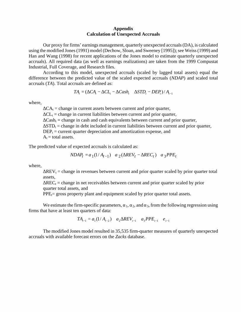
Appendix Calculation of Unexpected Accruals

Our proxy for firms’ earnings management, quarterly unexpected accruals (DA), is calculated

using the modified Jones (1991) model (Dechow, Sloan, and Sweeney [1995]); see Weiss (1999) and Han and Wang (1998) for recent applications of the Jones model to estimate quarterly unexpected accruals). All required data (as well as earnings realizations) are taken from the 1999 Compustat Industrial, Full Coverage, and Research files.

According to this model, unexpected accruals (scaled by lagged total assets) equal the difference between the predicted value of the scaled expected accruals (NDAP) and scaled total accruals (TA). Total accruals are defined as:

1/)( −−∆+∆−∆−∆= ttttttt ADEPSTDCashCLCATA

where, ∆CAt = change in current assets between current and prior quarter, ∆CLt = change in current liabilities between current and prior quarter, ∆Casht = change in cash and cash equivalents between current and prior quarter, ∆STDt = change in debt included in current liabilities between current and prior quarter, DEPt = current quarter depreciation and amortization expense, and At = total assets.

The predicted value of expected accruals is calculated as:

ttttt PPERECREVANDAP 3211 )()/1( ααα +∆−∆+= −

where, ∆REVt = change in revenues between current and prior quarter scaled by prior quarter total assets, ∆RECt = change in net receivables between current and prior quarter scaled by prior quarter total assets, and PPEt= gross property plant and equipment scaled by prior quarter total assets. We estimate the firm-specific parameters, α1, α2, and α3, from the following regression using

firms that have at least ten quarters of data:

11312211 )/1( −−−−− ++∆+= ttttt PPEaREVaAaTA ε The modified Jones model resulted in 35,535 firm-quarter measures of quarterly unexpected

accruals with available forecast errors on the Zacks database.

Statistics Forecast Errors Unexpcted Accruals(1) (2) (3)

Number of Observations 33,548 33,548

Mean -0.126 -0.217

Median 0.000 0.023

Standard Deviation 0.995 5.600

Skewness -6.976 -1.399

Kurtosis 102.307 16.454

% Positive 47.6 50.8

% Negative 39.9 49.2

% Zero 12.5 0.0

P1 -4.202 -20.820

P3 -1.983 -11.547

P5 -1.333 -8.386

P10 -0.653 -4.574

P25 -0.149 -1.349

P75 0.137 1.350

P90 0.393 4.185

P95 0.684 7.148

P97 0.939 9.891

P99 1.594 15.945

Table 1

Descriptive Statistics on Forecast Errors and Unexpcted Accruals

This table provides descriptive statistics on forecast errors and unexpcted accruals. Forecast erroris reported earnings (per Zacks) minus the last consensus forecast of quarterly earnings issuedprior to earnings announcement scaled by price. Unexpcted accruals are the measure produced bythe modified Jones Model (expressed as a per share scaled by price).

Panel A: Percentage of small positive forecast errors that fall within ranks of prior return

0<FE≤ 0.05 0<FE≤ 0.1 0<FE≤ 0.2Lowest 13.4% 14.5% 15.2%

2 19.3% 19.1% 18.9%3 21.3% 21.5% 21.1%4 23.8% 23.0% 21.9%

Highest 22.1% 22.0% 23.0%

Highest - Lowest 8.7% 7.5% 7.9%p-value for difference in proportions 0.000 0.000 0.000

Num. of obs. in small positive forecast error region 2,724 5,446 8,704

Panel B: Percentage of small positive forecast errors that fall within ranks of prior market adjusted return, by sign of unexpected accruals

Negative UA Positive UA Negative UA Positive UA Negative UA Positive UA Lowest 5.9% 7.6% 6.8% 7.7% 7.2% 7.9%

2 9.4% 10.0% 9.1% 9.9% 8.7% 10.2%3 10.2% 11.2% 10.6% 10.9% 10.4% 10.7%4 11.8% 12.0% 11.0% 12.0% 10.4% 11.4%

Highest 11.4% 10.7% 10.6% 11.3% 11.3% 11.8%

Highest - Lowest 5.5% 3.2% 3.9% 3.6% 4.0% 3.8%p-value for difference in proportions 0.000 0.000 0.000 0.000 0.000 0.000

Num. of obs. in small positive forecast error region 1,323 1,401 2,619 2,827 4,177 4,527

Table 2Percentage of Small Positive Forecast Errors that Fall within Ranks of Prior Market Adjusted Return

Unconditionally (Panel A) and by Sign of Unexpected Accruals (Panel B)This table reports the percentage of small positive forecast errors (greater than zero and smaller or equal 0.05, 0.1, and 0.2, respectively) that fall within ranks of prior marketadjusted return (panel A) and similar percentage by sign of unexpected accruals (panel B). Forecast error is reported earnings minus the last consensus forecast of quarterlyearnings issued prior to earnings announcement scaled by price. Unexpected accruals are the measure produced by the modified Jones model as described in the appendix(expressed as unexpected accrual per share scaled by price). Prior market adjusted return is the return between 10 days after the last quarterly earnings announcement to 10days prior to current quarterly earnings announcement minus the return on the value-weighted market portfolio for the same period. Each rank of prior market adjustedreturns comprise 6,117 observations.

Rank of prior market adjusted return

Rank of prior market adjusted return 0 < FE ≤ 0.20 < FE ≤ 0.05

Percentage of small positive forecast errors

Percentage of small positive forecast errors by sign of unexpected accruals (UA)0 < FE ≤ 0.1

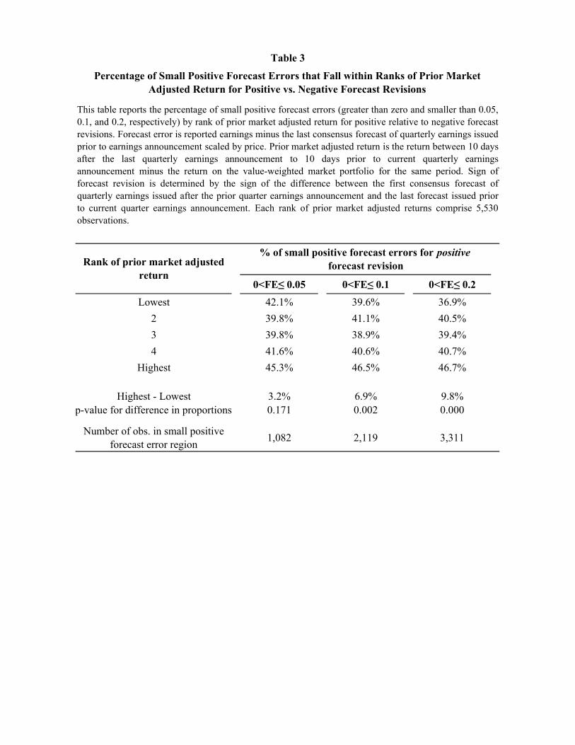
0<FE≤ 0.05 0<FE≤ 0.1 0<FE≤ 0.2Lowest 42.1% 39.6% 36.9%

2 39.8% 41.1% 40.5%3 39.8% 38.9% 39.4%4 41.6% 40.6% 40.7%

Highest 45.3% 46.5% 46.7%

Highest - Lowest 3.2% 6.9% 9.8%p-value for difference in proportions 0.171 0.002 0.000

Number of obs. in small positive forecast error region 1,082 2,119 3,311

Table 3

Percentage of Small Positive Forecast Errors that Fall within Ranks of Prior Market Adjusted Return for Positive vs. Negative Forecast Revisions

This table reports the percentage of small positive forecast errors (greater than zero and smaller than 0.05,0.1, and 0.2, respectively) by rank of prior market adjusted return for positive relative to negative forecastrevisions. Forecast error is reported earnings minus the last consensus forecast of quarterly earnings issuedprior to earnings announcement scaled by price. Prior market adjusted return is the return between 10 daysafter the last quarterly earnings announcement to 10 days prior to current quarterly earningsannouncement minus the return on the value-weighted market portfolio for the same period. Sign offorecast revision is determined by the sign of the difference between the first consensus forecast ofquarterly earnings issued after the prior quarter earnings announcement and the last forecast issued priorto current quarter earnings announcement. Each rank of prior market adjusted returns comprise 5,530observations.

Rank of prior market adjusted return

% of small positive forecast errors for positive forecast revision

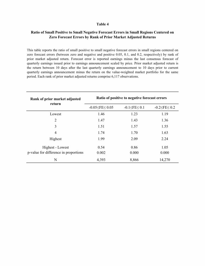
-0.05≤FE≤ 0.05 -0.1≤FE≤ 0.1 -0.2≤FE≤ 0.2

Lowest 1.46 1.23 1.192 1.47 1.43 1.363 1.51 1.57 1.554 1.74 1.70 1.63

Highest 1.99 2.09 2.24

Highest - Lowest 0.54 0.86 1.05p-value for difference in proportions 0.002 0.000 0.000

N 4,393 8,866 14,270

Rank of prior market adjusted return

Table 4

Ratio of Small Positive to Small Negative Forecast Errors in Small Regions Centered on Zero Forecast Errors by Rank of Prior Market Adjusted Returns

This table reports the ratio of small positive to small negative forecast errors in small regions centered onzero forecast errors (between zero and negative and positive 0.05, 0.1, and 0.2, respectively) by rank ofprior market adjusted return. Forecast error is reported earnings minus the last consensus forecast ofquarterly earnings issued prior to earnings announcement scaled by price. Prior market adjusted return isthe return between 10 days after the last quarterly earnings announcement to 10 days prior to currentquarterly earnings announcement minus the return on the value-weighted market portfolio for the sameperiod. Each rank of prior market adjusted returns comprise 6,117 observations.

Ratio of positive to negative forecast errors

Panel A: Percentiles of quarterly distributions of forecast errors

Panel B: Percentiles of quarterly distributions of unexpected accruals

Figure 1

Percentiles of Quarterly Distributions of Forecast Errors and Unexpected Accruals

This figure presents percentiles of quarterly distributions of analyst forecast errors (panel A) and unexpected accruals (panelB). Forecast error equals reported earnings minus consensus forecast of quarterly earnings issued prior to earningsannouncement scaled by beginning of period price. Unexpected accruals are the measure produced by the modified Jonesmodel as described in the appendix (expressed as unexpected accrual per share scaled by price).

*

-20

-16

-12

-8

-4

0

4

8

12

16

20

0 10 20 30 40 50 60 70 80 90

Percentiles of the unexpected accruals distributions

Most negative unexpected accruals

Most positive unexpected accruals

-6

-4

-2

0

2

4

6

0 10 20 30 40 50 60 70 80 90

Percentiles of the forecast error distributions

Most negative forecast errors

Most positive forecast errors

0

2

4

6

8

10

12

14

16

18

20

-0.5

0

-0.4

5

-0.4

0

-0.3

5

-0.3

0

-0.2

5

-0.2

0

-0.1

5

-0.1

0

-0.0

5

0.00

0.05

0.10

0.15

0.20

0.25

0.30

0.35

0.40

0.45

0.50

Forecast Errors

Perc

ent o

f for

ecas

t err

ors

Highest quintile of prior market-adjusted return

Lowest quintile of prior market-adjusted return

Figure 2 Histogram of Forecast Errors for Highest and Lowest Quintiles of Prior Market Adjusted ReturnPercent of forecast error values in histogram intervals for observations within forecast error of -.5 to +.5, for first and fifth quintiles of prior marketadjusted return. Forecast error is reported earnings (per Zacks) minus the last consensus forecast of quarterly earnings issued prior to earningsannouncement scaled by beginning of period price. Prior market adjusted return is the return between 10 days after the last quarterly earningsannouncement to 10 days prior to current quarterly earnings announcement minus the return on the value-weighted market portfolio for the sameperiod.

0

2

4

6

8

10

12

14

16

18

20

-0.5

00

-0.4

50

-0.4

00

-0.3

50

-0.3

00

-0.2

50

-0.2

00

-0.1

50

-0.1

00

-0.0

50

0.00

0

0.05

0

0.10

0

0.15

0

0.20

0

0.25

0

0.30

0

0.35

0

0.40

0

0.45

0

0.50

0

Forecast Errors

Perc

ent

Highest quintile of prior market-adjustedreturn and positive forecast revision

Highest quintile of prior market-adjustedreturn and negative forecast revision

Figure 3 Histogram of Forecast Errors for Highest Quintile of Prior Market Adjusted Return by Sign of Forecast RevisionPercent of forecast error values in histogram intervals for observations within forecast error of -.5 to +.5 for highest quintile of prior market adjusted return and then separated by the sign of the forecast revision. Forecast error is reported earnings (per Zacks) minus the last consensus forecast of quarterly earnings issued prior to earnings announcement scaled by beginning of period price. Prior market adjusted return is the return between 10 days after the last quarterly earnings announcement to 10 days prior to current quarterly earnings announcement minus the return on the value-weighted market portfolio for the same period. Sign of forecast revision is determined by sign of the first consensus forecast of quarterly earnings issued after prior quarter's earnings announcement and the last forecast issued prior to the current quarter earnings announcement.

Panel A: Percentage of extreme unexpected accruals that fall within ranks of prior market-adjusted returns

* Percentage of extreme accrual significantly different from all other portfolios.

Panel B: Percentage of extreme unexpected accruals within ranks of prior returns, by sign of forecast revision

Figure 4Percentage of extreme unexpected accruals within portfolios ranked on the basis

of prior market-adjusted return (Panel A) and by sign of forecast revision (Panel B)

Panel A depicts the percentage of extreme unexpected accruals that fall within portfolios ranked on the basis of prior market-adjustedreturn. Panel B depicts the percentage of extreme unexpected accruals that fall within these prior return portfolios by sign of analystearnings forecast revision. Extreme unexpected accruals observations are observations in the most negative (unconditional) decile ofunexpected accruals. Unexpected accruals are the measure produced by the modified Jones model as described in the appendix (expressedas unexpected accrual per share scaled by price). Prior market adjusted return is the return between 10 days after the last quarterly earningsannouncement to 10 days prior to current quarterly earnings announcement minus the return on the value-weighted market portfolio for thesame period. Sign of forecast revision is determined by the sign of the difference between the first consensus forecast of quarterly earningsissued after the prior quarter earnings announcement and the last forecast issued prior to current quarter earnings announcement.

16%

20%19%

28%

16%

0.00

0.05

0.10

0.15

0.20

0.25

0.30

0.35

Lowest 2 3 4 HighestPortfolios Ranked on the Basis of Prior Market-Adjusted Return

% o

f ext

rem

e un

expe

cted

acc

rual

s *

24%

15%

12% 11%

14%

4% 4% 4% 5%6%

0.00

0.04

0.08

0.12

0.16

0.20

0.24

Lowest 2 3 4 Highest

Portfolios Ranked on the Basis of Prior Market-Adjusted Return

% o

f ext

rem

e un

expe

cted

acc

rual

s % of extreme unexpected accruals for negative forecast revisions

% of extreme unexpected accruals for positive forecast revisions

Panel A: Percentage of extreme forecast errors within ranks of prior market-adjusted returns

* Percentage is significantly different from percentages in all other portfolios.

Panel B: Percentage of extreme forecast errors within ranks of prior returns, by sign of forecast revision

Figure 5Percentage of extreme forecast errors for portfolios ranked on the basis of

prior market-adjusted return (panel A) and by sign of forecast revision (Panel B)

Panel A depicts the percentage of extreme forecast errors that fall within portfolios ranked on the basis of prior market-adjusted return. Panel B depicts thepercentage of extreme forecast errors that fall within these prior return portfolios by sign of analyst earnings forecast revision. Extreme forecast errorsobservations are observations in the most negative (unconditional) decile of forecast errors. Prior market adjusted return is the return between 10 days afterthe last quarterly earnings announcement to 10 days prior to current quarterly earnings announcement minus the return on the value-weighted marketportfolio for the same period. Sign of forecast revision is determined by the sign of the difference between the first consensus forecast of quarterly earningsissued after the prior quarter earnings announcement and the last forecast issued prior to current quarter earnings announcement. Forecast error is reportedearnings minus the last consensus forecast of quarterly earnings issued prior to earnings announcement scaled by price.

34%

15% 16%14%

21%

0.00

0.05

0.10

0.15

0.20

0.25

0.30

0.35

0.40

Lowest 2 3 4 Highest

Portfolios Ranked on the Basis of Prior Market-Adjusted Return

% o

f ext

rem

e fo

reca

st e

rror

s

*

10% 11%9%

6% 5% 5% 5%4%

28%

16%

0.00

0.05

0.10

0.15

0.20

0.25

0.30

Lowest 2 3 4 Highest

Portfolios Ranked on the Basis of Prior Market-Adjusted Return

% o

f ext

rem

e fo

reca

st e

rror

s

% of extreme forecast errors for negative forecast revisions

% of extreme forecast errors for positive forecast revisions

Figure 6

Mean and median unexpected accruals for portfolios ranked on the basis of forecast errors within the lowest quintile of prior market-adjusted return

This figure depicts means and medians of unexpected accruals for portfolios ranked on the basis of forecasterrors within the lowest quintile of prior market-adjusted return. Unexpected accruals are the measure producedby the modified Jones model as described in the appendix (expressed as unexpected accrual per share scaled byprice). Prior market adjusted return is the return between 10 days after the last quarterly earnings announcementto 10 days prior to current quarterly earnings announcement minus the return on the value-weighted marketportfolio for the same period.

-2.0

-0.4

0.1 0.1

-0.10.0

-0.2

0.1

-0.5

-0.9

-0.1

0.1

0.3

0.1 0.00.1

0.1 0.10.0

-0.4

-2.20

-2.00

-1.80

-1.60

-1.40

-1.20

-1.00

-0.80

-0.60

-0.40

-0.20

0.00

0.20

0.40

Lowest 2 3 4 5 6 7 8 9 Highest

Portfolios Ranked on the Basis of Forecast Errors within the Lowest Quintile of Prior Market-Adjusted Return

Une

xpct

ed a

ccru

als

Mean unexpcted accruals

Median unexpcted accruals

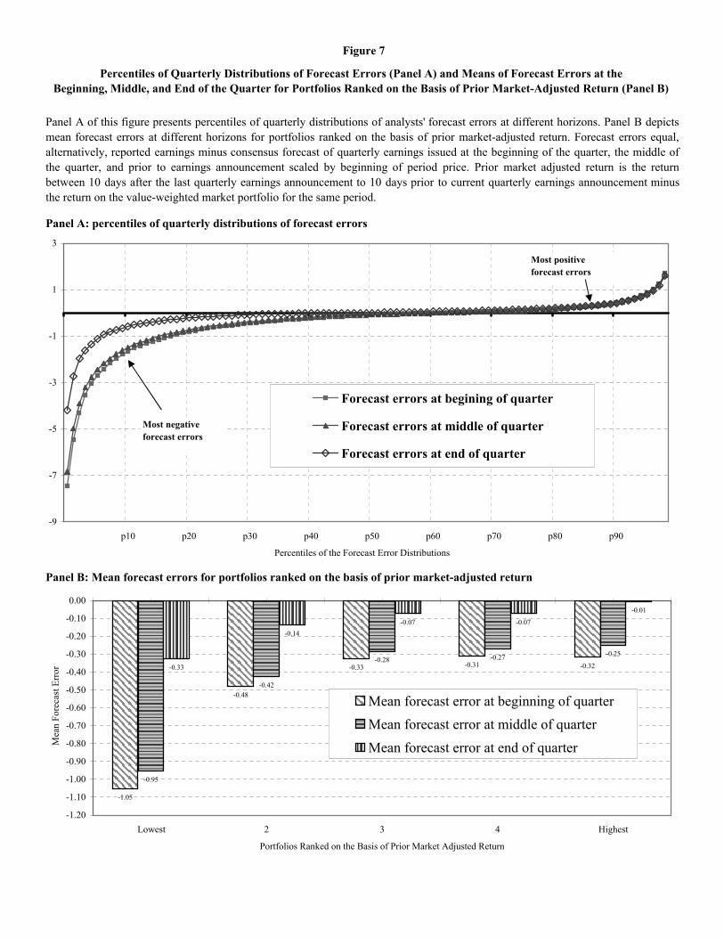
Panel A: percentiles of quarterly distributions of forecast errors

Panel B: Mean forecast errors for portfolios ranked on the basis of prior market-adjusted return

Figure 7

Percentiles of Quarterly Distributions of Forecast Errors (Panel A) and Means of Forecast Errors at the Beginning, Middle, and End of the Quarter for Portfolios Ranked on the Basis of Prior Market-Adjusted Return (Panel B)

Panel A of this figure presents percentiles of quarterly distributions of analysts' forecast errors at different horizons. Panel B depictsmean forecast errors at different horizons for portfolios ranked on the basis of prior market-adjusted return. Forecast errors equal,alternatively, reported earnings minus consensus forecast of quarterly earnings issued at the beginning of the quarter, the middle ofthe quarter, and prior to earnings announcement scaled by beginning of period price. Prior market adjusted return is the returnbetween 10 days after the last quarterly earnings announcement to 10 days prior to current quarterly earnings announcement minusthe return on the value-weighted market portfolio for the same period.

-9

-7

-5

-3

-1

1

3

p10 p20 p30 p40 p50 p60 p70 p80 p90

Percentiles of the Forecast Error Distributions

Forecast errors at begining of quarter

Forecast errors at middle of quarter

Forecast errors at end of quarter

Most negative forecast errors

Most positive forecast errors

-1.05

-0.48

-0.33 -0.31 -0.32

-0.95

-0.42

-0.28 -0.27 -0.25

-0.33

-0.07 -0.07

-0.01

-0.14

-1.20

-1.10

-1.00

-0.90

-0.80

-0.70

-0.60

-0.50

-0.40

-0.30

-0.20

-0.10

0.00

Lowest 2 3 4 Highest

Portfolios Ranked on the Basis of Prior Market Adjusted Return

Mea

n Fo

reca

st E

rror

Mean forecast error at beginning of quarterMean forecast error at middle of quarterMean forecast error at end of quarter

Panel A: Histograms of forecast errors

Panel B: Ratios of small positive to small negative forecast error at different horizons

Figure 8Histograms of Forecast Errors (Panel A) and Ratios of Small Positive to Small Negative Forecast Errors for

Portfolios Ranked on the Basis of Prior Market-Adjusted Return (Panel B) at the Beginning, Middle, and End of Quarter

Panel A of this figure presents histograms of forecast errors for observation within forecast error of -.5 to +.5. Panel B presents ratiosof small positive (within 0 to 0.1) to small negative forecast error (within 0 to -0.1) for portfolios ranked on the basis of prior market-adjusted return. Forecast errors equal, alternatively, reported earnings minus consensus forecast of quarterly earnings issued at thebeginning of the quarter, the middle of the quarter, and prior to earnings announcement scaled by beginning of period price. Priormarket adjusted return is the return between 10 days after the last quarterly earnings announcement to 10 days prior to currentquarterly earnings announcement minus the return on the value-weighted market portfolio for the same period.

0

2

4

6

8

10

12

14

16

18

20

-0.5

0

-0.4

5

-0.4

0

-0.3

5

-0.3

0

-0.2

5

-0.2

0

-0.1

5

-0.1

0

-0.0

5

0.00

0.05

0.10

0.15

0.20

0.25

0.30

0.35

0.40

0.45

0.50

Forecast Errors

Perc

ent

Percent of variable values in histograminterval at beginning of quarter

Percent of variable values in histograminterval at middle of quarter

Percent of variable values in histograminterval at end of quarter

0.97 0.95

1.13 1.091.20

0.911.04

1.12 1.15 1.191.23

1.571.70

2.09

1.43

0.00

0.50

1.00

1.50

2.00

2.50

Lowest 2 3 4 Highest

Portfolios Ranked on the Basis of Prior Market Adjusted Return

Rat

io o

f Sm

all P

ositi

ve to

Sm

all N

egat

ive

Fore

cast

Err

or

Ratio at beginning of quarterRatio at middle of quarterRatio at end of quarter

References Abarbanell, J., 1991, “Do Analysts’ Earnings Forecasts Incorporate Information in Prior Stock Price Changes?,” Journal

of Accounting and Economics 14, 147–165. Abarbanell, J., 2002, “A Framework for Analyzing Earnings Management: Implications for Stock Prices, Earnings and

Analysts’ Forecasts Errors," UNC, Working paper. Abarbanell, J., and R. Lehavy, 2002, "Differences in Commercial Database Reported Earnings: Implications for

Empirical Research," UNC/University of Michigan, Working paper. Abarbanell, J., and R. Lehavy, 2003a, “Can Stock Recommendations Predict Earnings Management and Analysts'

Earnings Forecast Errors?” Journal of Accounting Research, March. Abarbanell, J., and R. Lehavy, 2003b, “Biased Forecasts or Biased Earnings? The Role of Reported Earnings in

Explaining Apparent Bias and Over/Underreaction in Analysts’ Earnings Forecasts “, Working Paper. Basu, S., and S. Markov, 2003, “Loss Function Assumptions in Rational Expectations Tests on Financial Analysts'

Earnings Forecasts”, Working Paper, Emory University. Brown, L., 1993, “Earnings Forecasting Research: Its Implications for Capital Markets Research,” International Journal

of Forecasting, 295–320. Burgstahler, D., and M. Eames, 2000, “Management of Earnings and Analyst Forecasts,” Working paper, University of

Washington. Conrad, J., B. Cornell, and W. Landsman, 2002, “When Is Bad News Really Bad News?", Journal of Finance, 57, 2507-

2532. Dechow, P., and D. Skinner, 2000, "Earnings Management: Reconciling the Views of Accounting Academics,

Practitioners, and Regulators," Accounting Horizons, June 2000, 235-250. Dechow, P., R. Sloan, and A. Sweeney, 1995, “Detecting Earnings Management,” Accounting Review 70, 193–225. Degeorge, F., J. Patel, and R. Zeckhauser, 1999, “Earnings Management to Exceed Thresholds,” Journal of Business 72,

1–33. Finger, C., and W. Landsman, 1998, “What Do Analysts’ Stock Recommendations Really Mean?,” UNC, Working

paper. Fischer P., and R. Verrecchia, 2000, “Reporting Bias”, The Accounting Review, April 75(2): 229-245. Gu, Z., and J. Wu, 2003, “Earnings Skewness and Analyst Forecast Bias”, Journal of Accounting and Economics, April,

5-30. Han, J., and S. Wang, 1998, “Political Costs and Earnings Management of Oil Companies During the 1990 Persian Gulf

Crisis,” The Accounting Review 73, 103–118. Healy, P., and J. Wahlen, 1999, "A Review of the Earnings Management Literature and Its Implications for Standard

Setting," Accounting Horizons, 13, 365-383. Hribar, P., and D. Collins, 2002, “Errors in Estimating Accruals: Implications for Empirical Research,” Journal of

Accounting Research, Vol. 40 No. 1, 105-134.

Jones, J., 1991, “Earnings Management During Import Relief Investigations,” Journal of Accounting Research 29, 193–228.

Keane, M., and D. Runkle, 1998, “Are Financial Analysts’ Forecasts of Corporate Profits Rational?,” Journal of

Political Economy, 768–805. Kirschenheiter, M., and N. Melumad, 2002, “Can ‘Big Bath’ and Earnings Smoothing Coexist as Equilibrium

Financial Reporting Strategies?,” Journal of Accounting Research, vol. 40, no. 3, pp. 761-796. Kothari, S. P., 2001, “Capital Markets Research in Accounting,” Journal of Accounting and Economics 31, 105–232. Matsumoto, D., 1999, “Management’s Incentives to Influence Analysts’ Forecasts,” Harvard University, Working paper. Ohlson, J., 1999, “On Transitory Earnings”, Review of Accounting Studies, December, 145-162. Richardson, S., S. H. Teoh, and P. Wysocki, 1999, “Tracking Analysts’ Forecasts over the Annual Earnings Horizon:

Are Analysts’ Forecasts Optimistic or Pessimistic?,” Working paper, MIT. Skinner, D., and R. Sloan, 2002, “Earnings Surprises, Growth Expectations, and Stock Returns or Don’t Let an Earnings

Torpedo Sink Your Portfolio,” Review of Accounting Studies, 7, 289-312. Stickel, S., 1995, “The Anatomy of the Performance of Buy and Sell Recommendations,” Financial Analysts Journal,

51, 25–39. Verrecchia, R., 1986, “Managerial Discretion in the Choice Among Financial Reporting Alternatives,” Journal of

Accounting & Economics, 8, 175–195. Veronesi, P., 1999, “Stock Market Overreaction to Bad News in Good Times: A Rational Expectations Equilibrium

Model,” Review of Financial Studies, 12, 975–1007. Watts, R.L., 2002, “Conservatism in Accounting,” working paper, University of Rochester . Weiss, I., 1999, “Earnings Management in Response to a Transitory Earnings Shock,” Columbia University, Working

paper.