an experimental study of acoustic emission … experimental study of acoustic emission waveguides...

J. Acoustic Emission, 34 (2017) 12 ©2017 Acoustic Emission Group

An Experimental Study of Acoustic Emission Waveguides

Kanji Ono

Department of Materials Science and Engineering, University of California, Los Angeles

(UCLA), Los Angeles, CA 90095

Abstract

This study reports the characteristics of acoustic emission (AE) waveguides using displace-

ment pulse of about 1-µs duration from an ultrasonic transducer, driven by a short impulse. By

using one of broadband sensors as a receiver, improved characterization of waveguides is possi-

ble over 50 to 2000 kHz. Here, we obtained responses of circular rod waveguides of different

diameters from 1.6 to 12.7 mm with lengths varying from 60 to 900 mm. It is found that the low-

frequency part of L(0,1)-mode rod waves is dominant in thin rod waveguides. This mode is in-

creasingly suppressed above 6-mm diameter. This mode is also responsible for stretching a short-

duration (~1 µs) source into a long pulse of more than 100 µs as its velocity is reduced at higher

frequencies. At larger diameters, slower L(0,3)-mode becomes the dominant one, and its peak is

found at its highest velocity over a narrow range of frequency. To keep the pulse duration short,

it is necessary to keep the waveguide diameter below 3 mm, preferably at 1.6 mm or less so that

the relatively non-dispersive L(0,1)-mode prevails over the frequency range of interest. Diameter

reduction, however, leads to reduced sensitivity unless small aperture sensors are used. Tube

waveguides are found to offer a significant advantage of spectral smoothness. In tubes, L(0,2)

mode plays an important role of providing nearly constant velocity and spectral flatness. Effects

of threading are also evaluated. Three practical waveguide designs are suggested. More extensive

exploration of tubular waveguides is highly recommended.

Keywords: Waveguides, Rod waves, Tube waves, Threaded rods, Dispersion, Reverberation

Introduction

Waveguides have important roles in practical acoustic emission (AE) monitoring since the

earliest days. They are widely used in various industries, including petrochemical, electric power

generation, gas and oil transport, among others. Anderson et al. [1] reported their uses for fast

breeder reactors at the first conference on AE in 1971. Rods, tubes and wire bundles were al-

ready used in this work. Typical commercial waveguides are of stainless steel rod of 6 to 13 mm

in diameter and 300 mm in length, with or without a sensor mounting conical endpiece. They

may be welded to a structure to be monitored or with a pointed end for pressed contact. They are

also valuable in laboratory for conducting high or low temperature AE testing. For example, plat-

inum wire waveguide was used to detect oxide cracking and spallation at 1000˚C [2]. Various

references on rod wave propagation and mechanical waveguides can be found in literature [1,

3-7]. While the basic theory of rod waves was established over a century ago, more waveguide

related works are continuing [8, 9].

Our previous study evaluated waveguide characteristics of rods and tubes of different size

and length and concluded that commonly used 6-mm waveguide to be a good compromise in

terms of attenuation and signal broadening [3]. It was also suggested to keep the diameter small

and stay in the low frequency range to utilize the L(0,1)-rod-wave mode. Sikorska and Pan [10,

11] conducted extensive evaluation of short waveguides of several different materials relying on

Mor

e in

fo a

bout

this

art

icle

: ht

tp://

ww

w.n

dt.n

et/?

id=

2155

1

13

wavelet analysis as the main tool and compared their results with rod wave calculations. They

also examined traditional AE features. Perhaps most striking is the dominance of longitudinal

resonance due to the length values ranging from 18 to 177 mm. Hamstad [12] examined thin

waveguides of 1.6 mm in diameter using a high-fidelity NIST sensor and reported good repro-

duction of pencil-lead-break (PLB) induced plate waves through such waveguides, but with 11-

13 dB attenuation. A thicker (3.2 mm) waveguide produced less attenuation (–5 dB), but also

with less fidelity in waveform; i.e., more attenuation at higher frequencies. He evaluated plate

waves, dominated by low frequency A0-mode and the observed non-dispersive waves are appar-

ently due to the dominance of L(0,1)-rod-wave mode, noted earlier [3]. A more recent study of

Zelenyak et al. [13] introduced the finite element modeling (FEM) to the thin waveguide evalua-

tion, extending the Hamstad study and reproducing the essential features [12]. They showed that

FEM can be used in lieu of experiment allowing parametric study of waveguide behavior. Their

results show that a wave entering a waveguide exits with basically similar features. Attenuation

was low below 100 kHz, but tended to increase to about 10 dB at 1 MHz. It is noted, however,

that the frequency dependence of the simulated plate-wave signal of PLB is 40 dB/decade (from

0.1 to 1 MHz) after 100-mm propagation. This is twice that of the expected step-function source

used to simulate the PLB (with the rise time of 1 µs). As is well known, the calculated Fourier

transform of a step function has the inverse-frequency dependence (F = 2/j2πf). Accompanying

experimental result showed an even higher value of 50 dB/decade, which is 15 dB/decade higher

than that reported by Hamstad [12] in his comparable experiment. It is unclear why such discrep-

ancy arises from seemingly sound FEM methodology and essentially identical experimental set-

up, albeit different sensors. Because of the strong A0-mode plate waves, these PLB-based studies

inadvertently focus on the low frequency segment. It is hoped that future FEM work can reveal

the frequency dependence of amplitude attenuation in waveguides quantitatively.

In order to clarify the waveguide behavior under well-defined conditions, qualitative wave

propagation experiments were conducted using waveguides of three different materials, as well

as various diameter and length combinations. Three types of rods are included; solid round rods,

threaded rods and tubes. Previously, the facial displacement of an ultrasonic transducer was

characterized under pulse input [14]. That work used a step-down pulse, but this time the pulse-

generator output was shunted with 50-ohm load, achieving a shorter impulse output of ~1 µs du-

ration. The displacement waveform was measured using a laser interferometer. This displace-

ment pulse is sent through a waveguide under test and the displacement on the other end is de-

tected using a broadband sensor. The received signal is then analyzed using an FFT routine and

Choi-Williams transform to evaluate the waveguide characteristics. This study first reports the

time-frequency distribution of received signal intensity, and identifies the wave mode when it

can be established by a comparison to theoretical dispersion curves of rod and tube waves. It is

aimed to provide general view of wave propagation behavior in the size range for practical AE

waveguide applications. Next, the insertion loss (or attenuation) and reverberation (or multiple

reflections) effects are evaluated since these two have to be balanced to obtain workable wave-

guides. That is, a low-loss waveguide has extended reverberation, limiting it to applications with

low AE event rates. Some practical approaches are suggested.

Experimental

The source of displacement pulse utilized an ultrasonic transducer (AET FC500), which is

identified as 19-mm diameter element at 2.25 MHz center frequency. This was driven by an im-

pulse shown in Fig. 1 a) with the rise time of 50 ns, peak voltage of 225 V, decay time of

14

3 µs. We used a laser interferometer (Thales Laser S.A. SH-140) at Aoyama Gakuin University

(AGU). It has dc-20 MHz bandwidth as noted previously [14]. The displacement normal to the

front face is shown in Fig. 1 b), with the peak at 7.6 nm, returning to zero within 1.5 µs, followed

by low level oscillations to 30 µs. The rise time of the displacement pulse is 0.26 µs (or 0.16 µs

if 10%-90% value is used). The FFT result for the entire waveform of 30 µs length is given in

Fig. 1 c, showing adequate spectral intensity extending to 1.2 MHz and beyond at reduced inten-

sity. This FFT used Noesis (ver. 5.8) with 64-k points at 100 MHz sampling and the result is giv-

en as FFT magnitude spectrum in dB. The original signal was recorded at 500 MHz. Most other

FFT used 256-k points at 500 MHz. Note that when a step pulse is used to drive the FC500, the

initial pulse waveform was identical, but a tail extended for 10 µs (see Fig. 2 c) in [14]). This

produces unwelcome low frequency components in the present experiment. Also used as the

source of displacement pulse were Olympus V103, 1 MHz, 12.7-mm diameter transducer and

KRN BB-PCP conical sensor.

Fig. 1 a) Excitation pulse. b) Displacement output from FC500.

15

Fig. 1 c) FFT magnitude of the displacement output.

Fig. 2 Output waveform from KRN sensor, coupled to FC500 in face-to-face arrangement.

The displacement sensor utilized one of two broadband transducers. The primary receiver

was KRN (BB-PC), which is based on NIST-originated conical element sensor with compact

backing. This is a small aperture sensor of about 1 mm in diameter. Olympus V103 (or NDT

Systems C16. 2.25 MHz) with 12.7-mm element was also used to represent the displacement of

the entire end surface. When the KRN sensor is in contact with the source transducer (FC500), or

the face-to-face arrangement, the output of KRN receiver is shown in Fig. 2. This closely follows

the input waveform of Fig. 1 b) with the main pulse width of 1 µs. There is a low-level tail to 25

µs, however. The Choi-Williams transform (CWT) was applied on the KRN sensor output and

the result in a frequency-time-intensity plot or CWT spectrogram is given in Fig. 3. AGU-Vallen

Wavelet software was used for this operation. Peak intensity is found at 0.85 µs and covers the

range of 300 to 650 kHz, but signal intensity is present from 50 to 1800 kHz. In the following,

however, the discussion is mostly limited to 1500 kHz as the higher frequency range is usually

not of interest in waveguide applications.

16

Fig. 3 Frequency-time-intensity plot or spectrogram of Choi-Williams transform (CWT) of KRN

output in Fig. 2.

TheFFTofthereceivedsignalisgiveninFig.4asKRNsensorresponse,showing±6dB

flatnessover50 to1200kHz.When theFC500spectrum is subtracted fromtheKRNre-

sponse,wegetKRNsensorresponse,shownbyagreencurveinFig.4.Thispartwasdis-

cussedinaseparatereport[15],andshowedabroadbandresponseover50to1800kHz

(±6dB).Notethatthe V103 sensor has a similar response as this KRN sensor [15].

For the characterization of a waveguide, it is placed between the transmitter (FC500) and the

receiver (KRN-PC) except as noted. Vaseline petroleum gel was used as couplant. In the follow-

ing, we present the Choi-Williams transform applied on the KRN sensor output for each wave-

guide examined. Such time-frequency spectrograms are compared with the rod wave dispersion

curves, obtained using Disperse software. One example is given here for an aluminum rod of 6.4-

mm diameter in Fig. 5. It shows the group velocities of ten longitudinal L(0,x) and flexural

F(1,x) modes with x of 1 to 5. This leads to the identification of the wave modes present. When

different values of rod diameter are used, the horizontal scale needs modification. For double the

diameter, the frequency should read half the value shown here. For example, L(0,2) peak (green

curve) will be at 400 kHz for 12.8-mm diameter Al rod, instead of 800 kHz shown in Fig. 5. At-

tenuation can be estimated by comparing the observed spectrum with Fig. 4, although this part is

skipped, since the main aim is to find the general propagation behavior of waveguides. For the

evaluation of attenuation and signal broadening, it is best to use narrow-band signals as in Ref.

[8].

17

Fig. 4 FFT magnitude of the received signal or KRN sensor output (V) in purple, FC500 dis-

placement output (nm) in red, and KRN sensor response (V/nm) in green vs. frequency.

Another set of dispersion curves are calculated for tube waveguides. Figure 6 shows two of

them; Fig. 6 a) is for Al (Vp = 6.32 mm/µs, Vs = 3.13 mm/µs) with outer diameter/thickness (D/t)

ratio of 8.0, showing three L-mode velocities. Here, thickness is meant as the wall thickness.

Figure 6 b) is for Fe (Vp = 5.95 mm/µs, Vs = 3.26 mm/µs) with D/t = 4.0. In both cases, L(0,1)

velocity dips sharply near the cut-off frequency for L(0,2) mode. For Al, these values are 0.23

and 0.25 MHz·mm and, for Fe, 0.57 and 0.61 MHz·mm. Initially, L(0,1) velocity is near the rod

velocity, then L(0,2) mode has comparable velocity over a wider range of frequency-thickness

(f·t) product. For Fe, tube wave velocity exceeds 5 mm/µs at f·t < 0.26 MHz·mm and for 0.92 <

f·t < 1.42 MHz·mm.

Waveguides of aluminum, copper alloys and steels were used. Material composition of most

rods is unknown as cut rod samples typically come without identification or chemical analysis.

Most aluminum rods are believed to be Al 1100, except for 6.4 or 12.7 mm diameter rods of Al

2024. Four brass rods are expected to be C260, but two copper brazing alloys are of unknown

composition. From their densities, the alloy is presumed to be CP-3 (90Cu-2Ag-7P). Thinner

steel rods are of 1080 steel, while some are HSLA and stainless steels of unknown composition.

The longitudinal wave velocity can be obtained from the fastest arrival time along with the rod

wave velocity and mass density from sample weight. Thus, the elastic properties can be estimat-

ed when needed. Table 1 lists the materials and dimensions of waveguides used. The diameter

ranges from 1.6 mm to 12.7 mm, while the length varied from 59 mm to 913 mm. Tubes of the

same materials were also included in the study. Many of them were from our previous work [3].

The ends of these waveguides were polished down to 600-grit sandpaper using a jig.

18

Fig. 5 The dispersion curves of group velocity of rod waves in Al rod of 6.4-mm diameter.

Fig. 6 The dispersion curves for tube waveguides of Al and steel with diameter-to-thickness ra-

tio of 8.0 or 4.0, respectively.

19

Table 1 Waveguide materials and shape

Material Shape Size Length .

Al rod 1.6 mm ø 305 mm

rod 2.36 mm ø 305 mm








rod 9.6 mm ø 60, 151, 304 mm


rod 12.7 mm ø 150, 305, 611 mm

tube 7.9 mm/1.0 mm 152, 290 mm

tube 10.0 mm/1.1 mm 291 mm

Steel rod 1.6 mm ø 304 mm


Rod 3.2 mm ø 71, 165, 210, 238, 300 (238*) mm



rod 6.4 mm ø 150, 383 mm

rod 7.8 mm ø 59, 648 mm

rod 8.0 mm ø 350, 414 mm



rod 4-40 thread 305 mm

rod 6-32 thread 307 mm

rod ¼”-20 thread 383 (248ª) mm

rod ½”-13 thread 306 mm

tube 4.8 mm/0.73 mm 298, 377 mm

tube 6.4 mm/0.8 mm 168 mm

tube 6.4 mm/1.45 mm 90, 393 mm

tube 9.7 mm/1.3 mm with thread of 0.91 mm pitch, 543 mm

Cu rod 2.0 mm ø 100, 241, 411 mm

tube 6.4 mm/0.5 mm 88, 375 mm

tube 6.4 mm/0.76 mm 65, 100, 112, 198, 224, 525 (452ª), 626 mm

Brass rod 2.4 mm ø 305 mm


rod 4.8 mm ø (235ª) mm







Cu brazing rod 1.6 mm ø 200 mm

rod 2.36 mm ø 51, 149, 298 and 913 mm

Tube: Outer diameter/wall thickness

*: pointed end

ª: angled end face

20

Results and Discussion

1. Aluminum waveguides

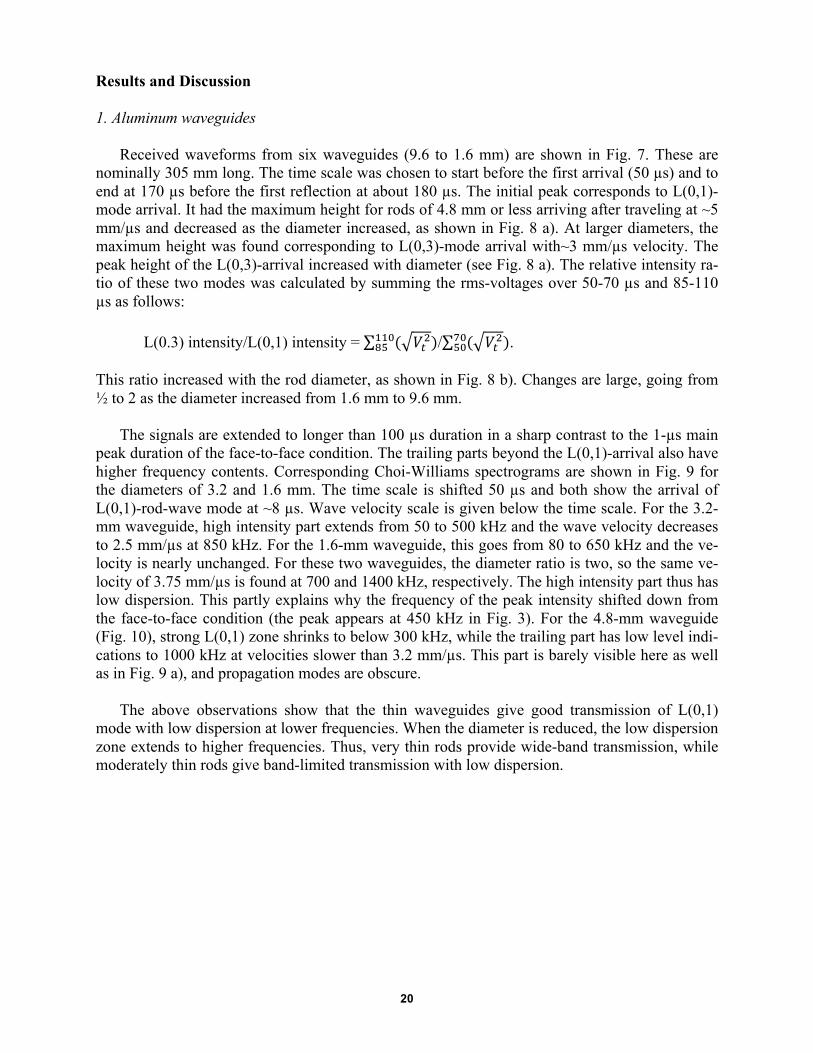
Received waveforms from six waveguides (9.6 to 1.6 mm) are shown in Fig. 7. These are

nominally 305 mm long. The time scale was chosen to start before the first arrival (50 µs) and to

end at 170 µs before the first reflection at about 180 µs. The initial peak corresponds to L(0,1)-

mode arrival. It had the maximum height for rods of 4.8 mm or less arriving after traveling at ~5

mm/µs and decreased as the diameter increased, as shown in Fig. 8 a). At larger diameters, the

maximum height was found corresponding to L(0,3)-mode arrival with~3 mm/µs velocity. The

peak height of the L(0,3)-arrival increased with diameter (see Fig. 8 a). The relative intensity ra-

tio of these two modes was calculated by summing the rms-voltages over 50-70 µs and 85-110

µs as follows:

L(0.3) intensity/L(0,1) intensity = ( �#$)&&'

() / ( �#$)*'

)' .

This ratio increased with the rod diameter, as shown in Fig. 8 b). Changes are large, going from

½ to 2 as the diameter increased from 1.6 mm to 9.6 mm.

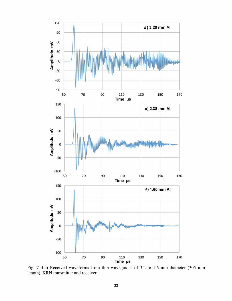
The signals are extended to longer than 100 µs duration in a sharp contrast to the 1-µs main

peak duration of the face-to-face condition. The trailing parts beyond the L(0,1)-arrival also have

higher frequency contents. Corresponding Choi-Williams spectrograms are shown in Fig. 9 for

the diameters of 3.2 and 1.6 mm. The time scale is shifted 50 µs and both show the arrival of

L(0,1)-rod-wave mode at ~8 µs. Wave velocity scale is given below the time scale. For the 3.2-

mm waveguide, high intensity part extends from 50 to 500 kHz and the wave velocity decreases

to 2.5 mm/µs at 850 kHz. For the 1.6-mm waveguide, this goes from 80 to 650 kHz and the ve-

locity is nearly unchanged. For these two waveguides, the diameter ratio is two, so the same ve-

locity of 3.75 mm/µs is found at 700 and 1400 kHz, respectively. The high intensity part thus has

low dispersion. This partly explains why the frequency of the peak intensity shifted down from

the face-to-face condition (the peak appears at 450 kHz in Fig. 3). For the 4.8-mm waveguide

(Fig. 10), strong L(0,1) zone shrinks to below 300 kHz, while the trailing part has low level indi-

cations to 1000 kHz at velocities slower than 3.2 mm/µs. This part is barely visible here as well

as in Fig. 9 a), and propagation modes are obscure.

The above observations show that the thin waveguides give good transmission of L(0,1)

mode with low dispersion at lower frequencies. When the diameter is reduced, the low dispersion

zone extends to higher frequencies. Thus, very thin rods provide wide-band transmission, while

moderately thin rods give band-limited transmission with low dispersion.

21

Fig. 7 a-c) Received waveforms from thin waveguides of 9.6 to 4.8 mm diameter (305 mm

length). KRN transmitter and receiver.

22

Fig. 7 d-e) Received waveforms from thin waveguides of 3.2 to 1.6 mm diameter (305 mm

length). KRN transmitter and receiver.

23

Fig. 8 a) Peak height of the initial arriving L(0,1)-mode signal (blue curve) and that of late arriv-

ing L(0,3)-mode signal (red curve). b) Ratio of L(0,3) and L(0,1) intensity vs. diameter.

24

Fig.9CWTspectrogramsforAlwaveguidesofa)3.2-andb)1.6-mmdiameter.Timescale

isshifted50µs.Groupvelocityvaluesaregivenbyverticalmarks.

25

Fig. 10 CWT spectrogram for Al waveguide of 4.8-mm diameter. Time scale is shifted 50 µs.

Group velocity values are given by vertical marks.

When the rod diameter reaches or exceeds 6.4 mm, higher rod-wave modes become visible,

as shown in Fig. 11. Here, the dispersion curves are shown on the left with the same frequency

scale, but the horizontal scales are different. L(0,1) mode is visible at low frequencies as shown

above and through its velocity minimum at 2.1 mm/µs. A new feature is a strong L(0,3) peak ap-

pearing at 3.1 mm/µs in the frequency range of 800 to 1100 kHz. Also visible are weak indica-

tions of L(0,2) and L(0,4). These identifications owe to a comparison to the rotated dispersion

curves shown on the left. These features are retained as the diameter is enlarged to 12.7 mm,

while keeping the length at nominally 305 mm (figure omitted). When the length is doubled, as

shown in Fig. 12, L(0,4) mode becomes stronger and L(0,5) is clearly noticeable. For the 6.4-mm

rod, shorter waveguides down to 66 mm showed the same features. However, in 9.6-mm or 12.7-

mm diameter rods, waveguides shorter than 150 mm produce much weaker L(0,1)-mode zone, as

shown in Fig. 13. Here, Fig. 13 a) is for 12.7-mm diameter rod of 152 mm and the main peak is

L(0,3) mode at 400-600 kHz. For the 9.6-mm rod (Fig. 13 b), L(0,3) position was at 550-850

kHz, proportionately higher. The weakening of L(0,1) is understandable as the wavelength at 100

kHz is 50 mm and the rod length is only three times the wavelength. Rod waves are constructed

by multiple interactions with the rod surfaces and a minimum length does exist at larger diame-

ters. Figure 14 indicates corresponding signal waveform of Fig. 13 b) and the peak amplitude

occurs at the time of L(0,3) peak. The waveform was omitted in Fig. 10, but the same trend was

observed. The presence of multiple wave modes contributes to the lengthening of the transmitted

signal as the maximum peak corresponds to the time of L(0,3) arrival. The waveform of 305-mm

long waveguide of the same 9.6-mm diameter was shown earlier in Fig. 7 a). While L(0,1) peak

height remained nearly the same, L(0,3) peak was about double at the half length.

26

Fig. 11 Dispersion curves for 6.4-mm waveguide (left) and observed CWT spectrogram (right).

Time scale is unshifted and group velocity values are given by vertical marks, covering 5 to 2

mm/µs.

Fig. 12 Observed CWT spectrogram for 12.7-mm Al waveguide (611 mm length). Time scale

was shifted by 98 µs for CWT. Original time scale and group velocity values are given by verti-

cal marks, covering 5 to 2 mm/µs.

Thicker waveguides develop higher rod-wave modes, L(0,3) in particular. This mode re-

quires less propagation distance to fully develop than the low-frequency L(0,1) mode, which

needs more than three-times the wavelength for rods of 9.6 mm or larger diameter. The transmis-

sion of L(0,3) mode can be utilized as a narrow-band mechanical filter and may be combined

with a resonating sensor design. For the range of diameter used here (6.4 – 12.7 mm), the

27

frequency range of 400 to 1100 kHz can be achieved. For 150-mm long rods, these ranges are:

6.4 mm, 800-1100 kHz; 9.6 mm, 500-750 kHz; 12.7 mm, 400-600 kHz.

Fig. 13 Observed spectrograms for 150-mm long Al waveguides of a) 12.7 and b) 9.6-mm diam-

eter. Group velocity values are given by vertical marks, covering 6 to 2 mm/µs.

Fig. 14 Signalwaveformof9.6-mmwaveguide,152-mmlength(Fig.13b)Thepeakampli-

tudecorrespondstoL(0,3)peak.

When hollow cylinders or tubes are used as waveguides, the transmission characteristics be-

come different from those of solid rods, as expected from the dispersion curves shown earlier

(Fig. 6). Figure 15 shows an example with an Al tube (9.5 mm OD, 7.5 mm ID, 290 mm length:

D/t = 9.5). The dispersion curves for D/t = 8 is shown as Fig. 15 a) for L(0,1) and L(0,2) modes.

(The cut-off frequency for L(0,3) mode is above 1.5 MHz). Results given in Fig. 15 b) match

with the dispersion curves well, with the peak L(0,2) activity at 350-800 kHz and the strongest

L(0,1) peak occurring at <100 kHz. The latter frequency is lower than the calculated values of

120-150 kHz. Extra peaks are also present between the two modes at 200 kHz with 4.3 to 4.8

28

mm/µs velocity. However, this frequency is at the minimum velocity for L(0,1) mode, where

FFT magnitude also shows a dip as will be discussed later. Thus, these peaks appear to be spuri-

ous although their origin is unknown. Wave intensity is reduced for slow moving waves: by 17

dB at >3 mm/µs. That is, signal lengthening is limited to <50 µs, a factor of 2 to 3 shorter than

rod waveguides of similar diameters.

In comparison to rod waveguide behavior (see for example, Figs. 11 and 12), the slow

L(0,3)-rod wave is gone. Instead, L(0,2)-tube wave behaves like the L(0,1)-wave for thin rods

with low dispersion. These are also beneficial for waveguide applications.

Fig. 15 a) The dispersion curves of tube waves for D/t = 8 with t = 1.18 mm. b) Observed CWT

spectrogram for Al tube (9.5 mm OD, 7.5 mm ID, 290 mm length: D/t = 9.5).

Although ten other tubes of various sizes were examined from a previous work [3], no clear

patterns emerged. L(0,1)-mode was always present and strongest, while L(0,2)-mode was absent

in some conditions. Even when 12.7-mm diameter tubes are used, we did see L(0,1) at low fre-

quency in contrast to solid rod cases where only L(0,3)-rod waves were found. When a low fre-

quency waveguide of large diameter is needed, a tube provides a solution. When L(0,2) is absent,

effects of the spurious peaks are significant and further study is needed to clarify their origin.

2. Steel Waveguides

The rod wave velocities of steel and aluminum are comparable; 5.06 vs. 5.18 mm/µs [5, p.

78]. However, Poisson’s ratio is smaller for iron and steel (0.29) than in aluminum (0.34) and

lateral stiffness is higher in steel. This is expected to affect how rod waves develop in steel, spe-

cifically, in the transition from the L(0,1)-dominated thin-rod behavior to multi-mode thick-rod

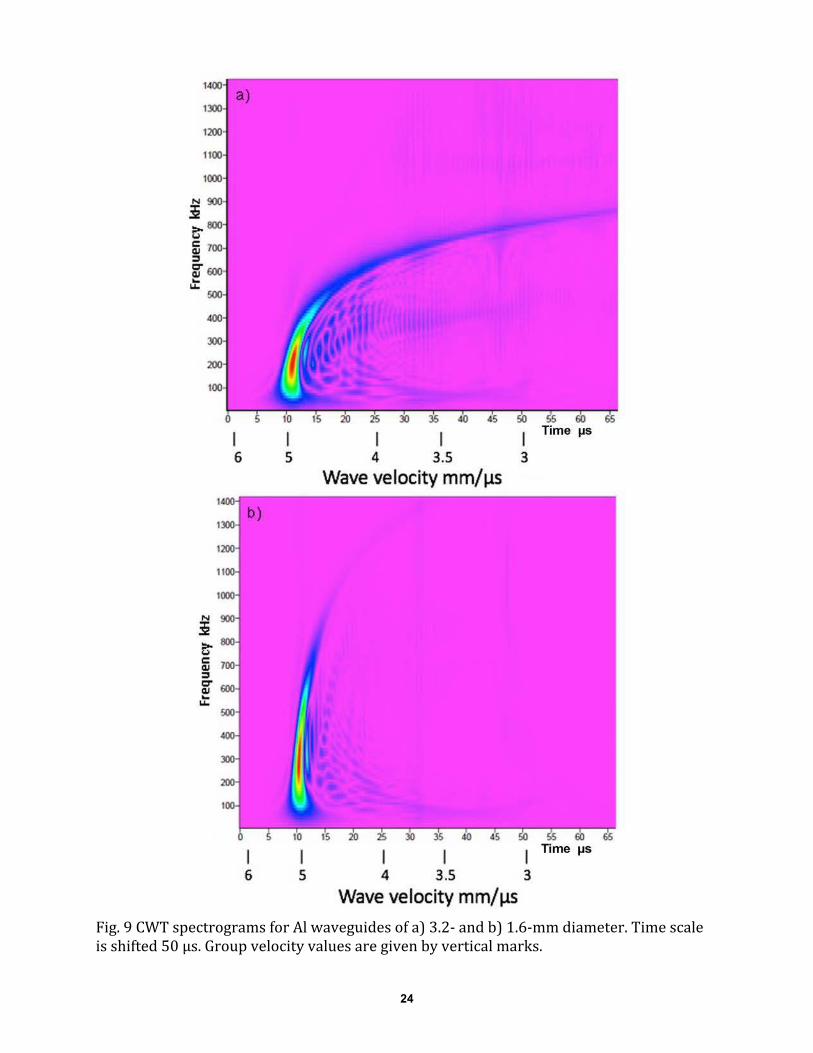
behavior. Dispersion curves for steel of 2.7-mm diameter are given in Figure 16 [15]. Figure 17

gives the CWT spectrogram for 6.4-mm diameter steel rod of 383-mm length, showing the thin-

rod behavior with mostly L(0,1) mode and weak L(0,3). This L(0,3) essentially disappeared at

496-mm length. In an aluminum waveguide of the same diameter, the L(0,3) mode was already

well developed, as was shown in Fig. 11.

29

Fig. 16 Dispersion curves for steel of 2.7-mm diameter from Mijarez (2014).

It is interesting to note that this diameter - length combination is commonly found in indus-

trial applications. Two commercially available waveguides from PAC and AECI share these di-

mensions – ¼” x 12” in the traditional US unit. From the present results, these waveguides work

best in the range up to 250 kHz, making them suitable for the often used frequency of 150 kHz.

In the previous study [3], we did conclude that this diameter is appropriate for industrial wave-

guide applications, although we only evaluated aluminum.

When a higher frequency detection is required, thinner waveguides offer the solution. At 4.8-

mm diameter, one obtains L(0,1) response to 400 kHz and to 550 kHz using 3.2-mm diameter

(similar to Fig. 9 a) for 3.2-mm Al). Using 1.6-mm steel rod, the response is comparable to Al

case of the same diameter (Fig. 9 b), except the signal strength drops off slightly faster than in Al.

In this case, low dispersion response to 600 kHz is possible.

When the length was halved to 150 mm for the 6.4-mm rod, the L(0,1) mode failed to devel-

op fully at frequency below 200 kHz (Fig. 18). This is a significant drawback in practical appli-

cation since oft-used 150-kHz AE sensor’s peak sensitivity is missed. The limitation posed by

the use of a certain length needs to be explored when the diameter approaches the transition to

multi-mode behavior.

When one examines these two spectrograms (Figs. 17 and 18), it is obvious that L(0,1) mode

in the short waveguide extends to higher frequency (600 kHz compared to 400 kHz) at slow

speed limits observed. This appears to indicate that the calculated dispersion curves, such as the

one shown in Fig. 5, are not applicable to short length rods. This is a reflection of inadequate de-

velopments of various wave modes. This part requires verification through future FEM calcula-

tions.

30

Fig. 17 Observed CWT spectrogram for steel waveguide of 6.4-mm diameter (383 mm length).

Time shift = 70 µs.

Fig. 18 Observed CWT spectrogram for a short steel waveguide of 6.4-mm diameter (150 mm

length). Time shift = 25 µs.

Steel waveguides exhibit another behavior during the transition. Multi-mode behavior is

found once the diameter reaches ~8 mm. For 7.8-mm diameter, L(0,3) mode is dominant from a

short rod (59 mm) to a long one (648 mm). At 59 mm length, modes are not as clearly separated,

but showing both L(0,1) and L(0,3) as well as possibly L(0,2) spots (Fig. 19). Figure 20 shows

the nearly single L(0,3)-mode behavior that evolved in longer waveguides. This observation

points to the needs of considering the waveguide design from both the diameter, which is of

course the main parameter, and also the length. Since the partition of energy transmission into

various modes cannot be theoretically predicted at present, we need to evaluate individual wave-

guide design to ascertain its performance.

31

Fig. 19 Observed waveform and CWT spectrogram for a short steel waveguide of 7.8-mm di-

ameter (59 mm length). The reflected waves appear starting at 34 µs.

Fig. 20 Observed waveform and CWT spectrogram for a long steel waveguide of 7.8-mm diame-

ter (648 mm length).

32

Fig. 21 a) The dispersion curves of tube waves for D/t = 4 with t = 1.6 mm. b) Observed CWT

spectrogram for a steel tube (6.4 mm OD, 3.3 mm ID, 394 mm length: D/t = 3.7). Group velocity

values are given by vertical marks, covering 5 to 3.7 mm/µs.

In testing tube waveguides of steel, four tube sizes were available with the outer diameter of

4.8 and 6.4 mm and D/t ratio of 3.7 to 8. These are of austenitic stainless steel, presumably of

304 type. Main response was L(0.1)-and L(0,3), similar to the case for Al tube (Fig. 15). For a

long heavy wall 6.4-mm tube (D/t = 3.7; 394 mm length), Fig. 21 shows the CWT spectrogram

together with the calculated dispersion curves. L(0,2) velocity agrees well with the calculated

values, while L(0,1)-mode shows lower frequency at a given velocity. The highest received in-

tensity corresponds to L(0,2) mode here with D/t = 4, while it was L(0,1) mode in the case of Al

with D/t = 8 (cf. Fig. 15). Note that spurious peaks are again seen at 300-500 kHz over 8-10 µs in

this shifted time scale.

When the tube diameter is reduced to 4.8 mm with D/t = 6.6, the dispersion of L(0,2) mode is

reduced as shown in Fig. 22 a). The position of L(0,1) peak is similar to Fig. 21, but its intensity

is stronger. The middle spectrogram (Fig. 22 b) is for the same diameter of 6.4 mm, but with a

thinner wall or D/t = 8 and at less than a half-length. Here, L(0,1) is absent and only the L(0,2)

mode is found from 400 to 1100 kHz. This is a beneficial effect of a shorter length, which is be-

low the minimum length needed for developing the L(0,1) mode. In Fig. 22 c), a similar result is

exhibited with another short waveguide of 6.4 mm: D/t = 3.7 (the same tube for Fig. 21) and the

length of 90 mm. This effect was also observed in Al cases.

34

Fig. 22 Observed CWT spectrograms for steel tubes. a) tube diameter = 4.8 mm; D/t = 6.6 (377

mm length). b) tube diameter = 6.4 mm; D/t = 8 (168 mm length). c) short (90 mm) waveguide

of 6.4 mm: D/t = 3.7. Time shift is marked in the figure.

From these cases, we find that tube waveguides are advantageous over rods of smaller di-

ameter in rejecting low frequency components. It appears that a large D/t ratio enhances L(0,2)-

mode, as was found in Al tube waveguides. The same high-pass filtering effect can be obtained

by using a shorter waveguide as L(0,1) mode requires a certain minimum length to develop. This

length appears to be about 5-times the wavelength.

3. Copper Alloys

For this group, copper rods (of three different lengths), two copper tubes, brass rods (of five

different diameters), brass tubes (of four different diameters) and two copper brazing alloy rods

were used. All the rods are thin, the maximum diameter being 5.3 mm and their wave propaga-

tion behavior mostly resembled those of thin Al rods. Poisson’s ratios of aluminum, copper, and

brass (30Zn-70Cu) are in the range of 0.32 to 0.36 and the lateral stiffness is comparable to each

other. The thin-rod behavior is observed for 305-mm length up to 4 mm in diameter and for 5-

mm-diameter brass rod of 200-mm length, but the multi-mode behavior is found for 5-mm brass

rod of 300-mm length.

The copper brazing alloy rods tested were identified by their mass density as CP-3 alloy with

90Cu-2Ag-7P composition. Diameters are 1.6 and 2.4 mm. Thinner 1.6-mm rod is of 200-mm

length, while thicker 2.4-mm rod samples have lengths of 51, 149, 298 and 913 mm. All of them

showed the thin rod behavior of single L(0,1) mode. Two examples are given in Fig. 23.

Of the two, the top graph approximates the condition used by Hamstad and Zelenyak [12, 13],

who used 1.6-mm diameter Cu wire. The observed CWT spectrogram shows that L(0,1) mode

has a nearly constant velocity to 450 kHz, the primary frequency range of their A0-mode plate

wave. For this range, this wire size gives good reproduction of input waveforms. At higher fre-

quencies, the wave velocity and transmitted amplitude decrease, as was observed in Hamstad’s

experiment. For 2.4-mm wire case, the flat response zone is reduced to less than 250 kHz and

34

waveform fidelity is reduced substantially. The high frequency velocity slow down and attenua-

tion also occur, commencing at 200 kHz.

Fig. 23 Observed CWT spectrograms for wires of a copper brazing alloy (type CP-3). a) 1.6 mm

diameter. 200 mm length. b) 2.36 mm diameter. 913 mm length. Group velocity values are given

by vertical marks, covering 4 to 2 mm/µs.

In copper tube testing, common 6.4-mm diameter copper refrigeration tubes were evaluated

as waveguides. The tube is available in wall thickness of 0.5 or 0.76 mm, giving D/t of 12.5 or

8.35. Basic features are identical to those of Al and steel, but Fig. 24 a) shows an example with a

large length (627 mm). This tube’s D/t was 8.35. Because of the length, both modes developed

fully. However, the spurious peaks showed up, centering at 250 kHz, corresponding to a dip in

FFT magnitude over 170-270 kHz. This large length does decrease the peak in waveform by 10

dB in comparison to shorter waveguides of 80 to 150 mm length.

35

A set of brass tubes are also examined. These tubes have the diameter of 4.8 to 6.4 mm and

the wall thickness of 0.4 mm, with D/t of 12 to 16. A representative CWT spectrogram is given

in Fig. 24 b). At higher D/t ratios, L(0,1) is reduced compared to the common 6.4-mm Cu tube.

Due to high D/t, this 4.8-mm tube is useful for 500-1300 kHz range with low dispersion. With a

larger diameter, the frequency range moves lower; to 400 to 1100 kHz for 6.4 mm diameter (D/t

= 16). Thus, we again observe with a tube waveguide the low dispersion L(0,2)-propagation

mode and the suppression of low frequency L(0,1) mode, giving a high-pass filtering effect.

Fig. 24 CWT spectrograms of copper and brass tube waveguides. a) copper, 6.4 mm diameter,

D/t = 8.35, 626 mm length. Time shift = 150 µs. b) brass, 4.8 mm diameter, D/t = 12, 305 mm

length. Time shift = 75 µs.

4. Threaded waveguides

Next series of tests are included in order to evaluate effects of surface condition on the prop-

agation of rod waves. Readily available surface modification is the use of threaded rods. The first

example is shown in Fig. 25. This is an Al rod with ¼”-20 thread (6.2 mm diameter-1.27 mm

pitch thread) of 305 mm length. Corresponding smooth rod CWT spectrogram is given in Fig. 11

(right graph), showing multi-mode transmission with strong L(0,1) and L(0,3) intensity. In con-

trast, Fig. 25 shows strong L(0,1) mode and much weaker L(0,3) mode in the threaded rod. Thus,

this waveguide behaves like a non-threaded rod of smaller diameter. In addition, the velocity of

the observed L(0,1) mode is approximately 10% slower than that of non-threaded rod: 4.77

mm/µs vs. 5.28 mm/µs. A much slower (~2.5 mm/µs) peak is present at the intersection of

L(0,1), F(1,2) and F(1,3). This was also found in Fig. 11, but their origin is unclear.

In contrast, Fig. 25 shows strong L(0,1) mode and much weaker L(0,3) mode in the threaded

rod. Thus, this waveguide behaves like a non-threaded rod of smaller diameter. In addition, the

velocity of the observed L(0,1) mode is approximately 10% slower than that of non-threaded

rod: 4.77 mm/µs vs. 5.28 mm/µs. A much slower (~2.5 mm/µs) peak is present at the intersec-

tion of L(0,1), F(1,2) and F(1,3). This was also found in Fig. 11, but their origin is unclear.

36

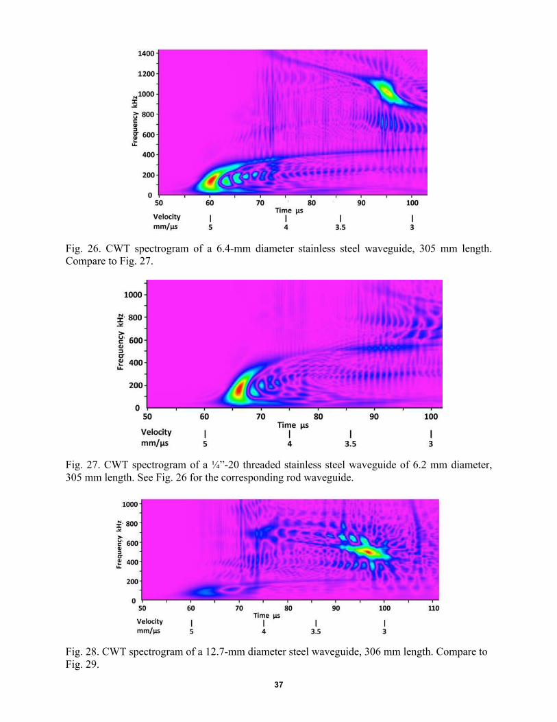
Figures 26 and 27 shows a comparable pair of stainless steel. Diameter is again 6.35 mm for

smooth rod and the thread is ¼”-20 with the length of 301 mm (6.2-mm diameter). Fig. 26 shows

the result of the non-threaded rod, indicating the presence of both L(0,1) and L(0,3) modes. Fig-

ure 26 is the threaded counterpart. L(0,3) mode was not observed as was the case for Al (cf. Fig.

25). Again, threading of rod suppressed the higher rod-wave mode.

When the rod diameter is increased to 12.7 mm using steel rod (length = 306 mm), the

threading effect was different from the 6.35-mm examples of Figs. 25 and 27. Figure 28 shows

the non-threaded case while Fig. 29 plots the threaded one. Thread is ½”-13 (12.7-mm nominal

diameter with 1.96 mm pitch). Figure 28 shows a strong L(0,3) mode, but weak L(0,1) and

L(0,4) are also present. With threading, L(0,3) remains the strongest, but L(0,1) becomes strong-

er second mode. That is, weakened L(0,3) and higher modes contributed to make L(0,1) more

prominent.

A similar trend is found in five other sets of threaded and non-threaded rods, indicating that

threaded rods enhance L(0,1) mode at the expense of higher L-modes. In most cases, threading

reduced the L(0,1) mode velocity by about 10%. In one case of brass, the velocity was nearly

unchanged. It is possible that compositions of the alloys are not identical because many brass

compositions are used in commercial applications, and the samples came from different sources.

These observations imply that the primary benefit of threaded rods as waveguides is to pro-

mote the lowest L mode while depressing higher modes. This may arise from reduced surface

reflectivity, but is also due to smaller effective diameter of the threaded rods.

Fig. 25. CWT spectrogram of a ¼”-20 threaded Al waveguide of 6.2 mm diameter, 305 mm

length. See Fig. 11 for the corresponding rod waveguide of 6.4 mm diameter.

37

Fig. 26. CWT spectrogram of a 6.4-mm diameter stainless steel waveguide, 305 mm length.

Compare to Fig. 27.

Fig. 27. CWT spectrogram of a ¼”-20 threaded stainless steel waveguide of 6.2 mm diameter,

305 mm length. See Fig. 26 for the corresponding rod waveguide.

Fig. 28. CWT spectrogram of a 12.7-mm diameter steel waveguide, 306 mm length. Compare to

Fig. 29.

38

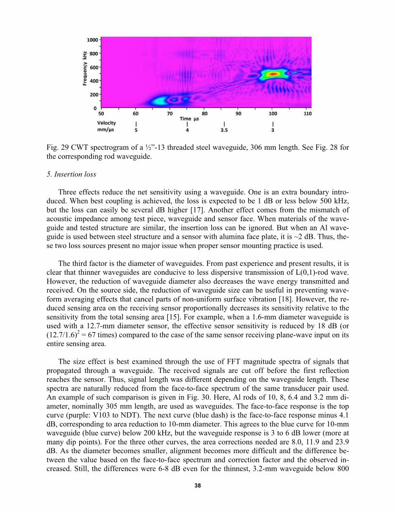
Fig. 29 CWT spectrogram of a ½”-13 threaded steel waveguide, 306 mm length. See Fig. 28 for

the corresponding rod waveguide.

5. Insertion loss

Three effects reduce the net sensitivity using a waveguide. One is an extra boundary intro-

duced. When best coupling is achieved, the loss is expected to be 1 dB or less below 500 kHz,

but the loss can easily be several dB higher [17]. Another effect comes from the mismatch of

acoustic impedance among test piece, waveguide and sensor face. When materials of the wave-

guide and tested structure are similar, the insertion loss can be ignored. But when an Al wave-

guide is used between steel structure and a sensor with alumina face plate, it is ~2 dB. Thus, the-

se two loss sources present no major issue when proper sensor mounting practice is used.

The third factor is the diameter of waveguides. From past experience and present results, it is

clear that thinner waveguides are conducive to less dispersive transmission of L(0,1)-rod wave.

However, the reduction of waveguide diameter also decreases the wave energy transmitted and

received. On the source side, the reduction of waveguide size can be useful in preventing wave-

form averaging effects that cancel parts of non-uniform surface vibration [18]. However, the re-

duced sensing area on the receiving sensor proportionally decreases its sensitivity relative to the

sensitivity from the total sensing area [15]. For example, when a 1.6-mm diameter waveguide is

used with a 12.7-mm diameter sensor, the effective sensor sensitivity is reduced by 18 dB (or

(12.7/1.6)2 = 67 times) compared to the case of the same sensor receiving plane-wave input on its

entire sensing area.

The size effect is best examined through the use of FFT magnitude spectra of signals that

propagated through a waveguide. The received signals are cut off before the first reflection

reaches the sensor. Thus, signal length was different depending on the waveguide length. These

spectra are naturally reduced from the face-to-face spectrum of the same transducer pair used.

An example of such comparison is given in Fig. 30. Here, Al rods of 10, 8, 6.4 and 3.2 mm di-

ameter, nominally 305 mm length, are used as waveguides. The face-to-face response is the top

curve (purple: V103 to NDT). The next curve (blue dash) is the face-to-face response minus 4.1

dB, corresponding to area reduction to 10-mm diameter. This agrees to the blue curve for 10-mm

waveguide (blue curve) below 200 kHz, but the waveguide response is 3 to 6 dB lower (more at

many dip points). For the three other curves, the area corrections needed are 8.0, 11.9 and 23.9

dB. As the diameter becomes smaller, alignment becomes more difficult and the difference be-

tween the value based on the face-to-face spectrum and correction factor and the observed in-

creased. Still, the differences were 6-8 dB even for the thinnest, 3.2-mm waveguide below 800

39

kHz. The main source of the insertion loss (excluding the area correction) is the lack of good

coupling due to poor alignment.

Another prominent feature of these waveguide spectra is the presence of many dips, especially

above the frequency corresponding to the velocity minimum of L(0,1)-mode wave. For these

four curves, the values are 330, 490, 600 and 1200 kHz. These rod spectra are relatively smooth

below the L(0,1) dip. Other large dips correspond to velocity minima of higher propagation

modes. However, many other dips have no clear origins.

Fig. 30 FFT magnitude spectra of signals propagated through Al waveguide of 10 (blue), 8 (red),

6.4 (green) and 3.2 (light blue) mm diameter, 305 mm length. Face-to-face response of V103-

NDT transducer pair is given by purple curve (top). Its area corrected response (minus 4.1 dB) is

shown by blue dashed curve.

The second example is a comparison between rod and tube waveguides, shown in Fig. 31.

Material is Al, with the same diameter of 8 mm. The red curve (same as the red one in Fig. 30) is

for a rod (8 mm ø x 305 mm), while the blue curve is for a tube (7.9-mm OD x 6 mm ID x 290

mm length). The red and blue dash curves are area-corrected ideal spectra from the face-to-face

data (purple curve). As before, 3 – 6 dB differences are found for the rod, while the tube data dif-

fer more above 200 kHz. A large dip exists centering at 240 kHz. This corresponds to the dip in

velocity for L(0,1) and the cut-off frequency of L(0,2) mode. Above this dip, the tube data is

much more smooth to 2 MHz. The flat spectrum zone from 300 to 900 kHz for the tube corre-

sponds to L(0,2) mode, but modes at higher frequencies are unknown at present. Still, this tube

spectrum is smoother than the rod spectrum at the same frequency.

The third example is 3.2-mm steel waveguides of differing length, 71, 165 and 238 mm. The

face-to-face and area corrected spectra are in purple in Fig. 32, while steel data are in blue (short),

red (medium) and green (long). The rod data are flat to 1 MHz, but differences are 10-20 dB.

Length effects are not obvious as coupling is more critical. This frequency range corresponds to

L(0,1) mode.

40

Fig. 31 FFT magnitude spectra of signals propagated through Al waveguide of 8 mm diameter,

305 mm length (red) and a tube of 7.9-mm OD, 6-mm ID, 290 mm length (blue). Face-to-face

response of V103-NDT transducer pair is given by purpl curve (top). Its area corrected responses

(minus 8.0 and 11.9 dB) are shown by red and blue dashed curves.

Fig. 32 Output spectra from 3.2-mm steel waveguides of length, 71 (blue), 165 (red) and 238

(green) mm. Face-to-face response of V103-NDT transducer pair is given by purple curve (top).

Its area corrected response (minus 19.5 dB) is shown by purple dashed curve.

41

Fig. 33 FFT magnitude spectra of signals propagated through steel waveguide of 6.4 mm diame-

ter, 382 mm length (red) and a tube of 6.4-mm OD, 3.5-mm ID, 393 mm length (blue). Face-to-

face response of V103-NDT transducer pair is given by purple curve (top). Its area corrected re-

sponses (minus 11.9 and 14.4 dB) are shown by red dash and blue dash curves.

The last example is a comparison between steel rod and tube of 6.4 mm diameter. Figure 33

shows the face-to-face and area-corrected spectra as top three curves. The rod (6.4 mm ø x 383

mm) is in blue, showing a dip due to the L(0,1) velocity cusp at 0.5 MHz. This is 5 to 8 dB be-

low the blue dash curve of the predicted spectrum. The dotted red curve is for the predicted spec-

trum for 6.4-mm tube (3.5 mm ID x 393 mm). The observed spectrum is shown in red. These

two match well below 300 kHz before reaching a dip due to L(0,1) dip/L(0,2) cut-off frequency

over 286-404 kHz). Beyond the dip, a differences of 3-6 dB are observed to 2 MHz. This zone

has a smooth spectrum.

These observations are also found in several other sets of rods, tubes, and their mix of differ-

ent length. Results are comparable over all. However, a few pairs of transducers produced more

attenuation in rods or tubes. The reason for this discrepancy is unknown at present.

6. Reverberation

Reverberation (or multiple reflections) is another important feature of waveguides that has to

be considered in their design. This effect has been recognized from the beginning of their usage.

Earlier waveguide studies [2, 10, 11] observed unwanted signal stretching, sometimes exceeding

10 ms. Sikorska and Pan [10, 11] examined angled face up to 60˚, but only 5 to 8 dB attenuation

was achieved. Ono and Cho [3] evaluated a pointed-end waveguide and found improved pulse

definition, but the suppression of multiple reflections was not addressed.

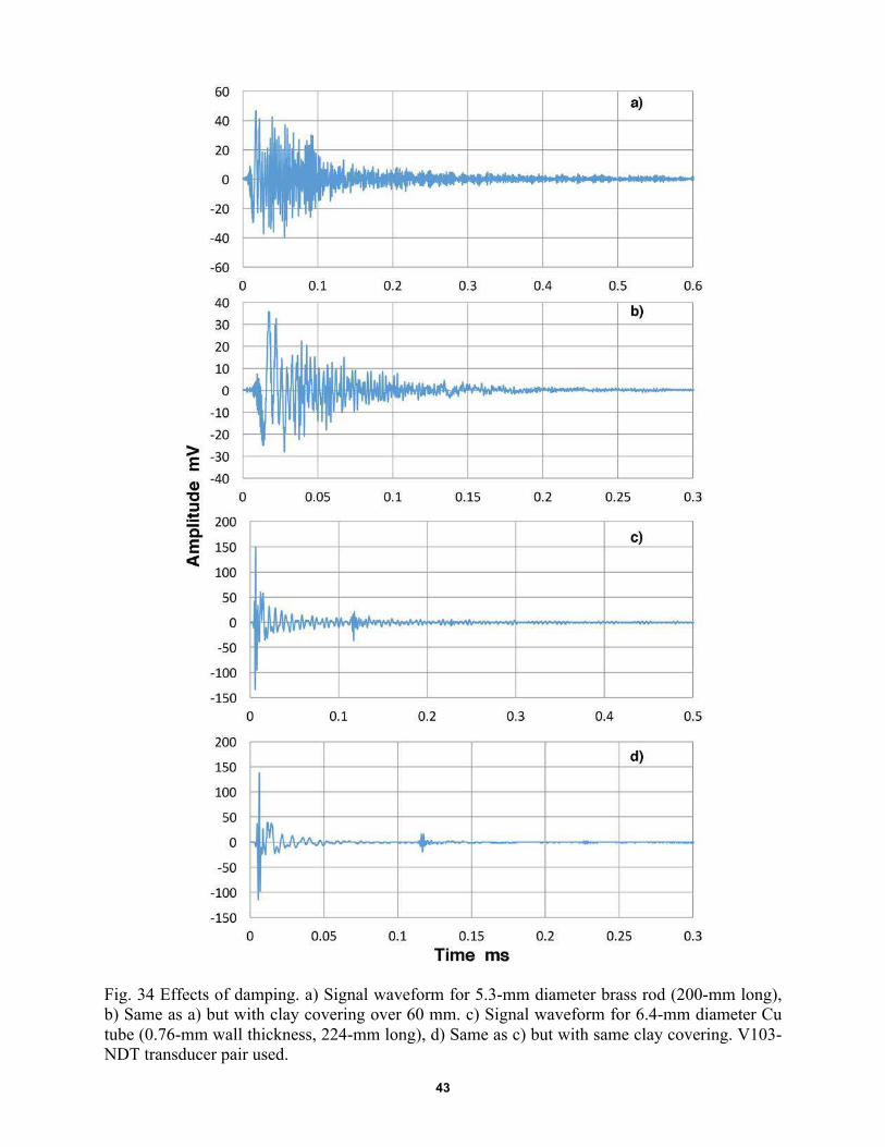
The first usual step one takes to suppress unwanted reflections is applying damping medium

on such waveguides. Examples are shown in Fig. 34 (using V103 transmitter, NDT receiver).

The top figure (Fig. 34 a) is the output signal from a brass rod (5.3 mm ø x 200 mm length),

42

lasting 0.5 ms to 20 dB down. Figure 34 b) shows the same rod, but its 60-mm length in the mid-

dle covered with clay (plumber’s putty, a mixture of natural clay and linseed oil). The signal

length is halved to 0.15 ms, while the peak amplitude decreased 2 dB. In both cases, reflections

are buried in the slow-moving signals. The third graph is for a Cu tube waveguide (6.4-mm di-

ameter, 0.76 mm wall thickness, 224 mm length), giving signal length of 0.12 ms. With clay ap-

plied in the middle, Fig. 34 d) results, with the same signal length but amplitude reduced beyond

0.04 ms. For these tube waveguides, the initial decay is large and reflections can be easily seen.

Again, clay damped slow-moving waves more than the initial pulse, which only decreased by 1

dB.

These signals can be represented by an exponential decay equation of

V = Vo exp[–a(t – to)],

where Vo is the initial peak, a decay constant and to signal arrival time. For these four signals, we

obtain decay constant a of 3.2, 7.6, 5.9 and 7.3 in the unit of ms–1

. These show that tube is more

effective in reducing higher mode waves, and obtain better damping effects from surface absorb-

er like clay. As noted before, L(0,3)-rod wave is strong in Fig. 34 a) while L(0,1)-tube wave is

dominant in Fig. 34 c).

The increased decay constants resulted from the reduction in slow moving L(0,1) and L(0,3)

modes. The CWT spectrogram of the rod (Fig. 34 a) is similar to Figs. 17 and 26 for 6.35-mm

steel rods, while the rod with clay damper resembles threaded steel rod (Fig. 27). The spectro-

grams for tubes with or without clay are similar to Fig. 24 a), except the velocity slow-down at

high-frequencies is absent. Their signal spectra are given in Fig. 35, with the red curves showing

the effects of clay damping. The top curves (Fig. 35 a) are for the rod cases, indicating essential-

ly no amplitude loss from clay below 200 kHz but the loss increasing above 300 kHz. The higher

frequency parts are barely present in the CWT spectrograms as they are spread over time. Figure

35 b) is for the tube cases. Here, amplitude loss appears only above 1 MHz, reflecting a small

reduction in the peak amplitude (see Fig. 34 c and d). Slower segment of L(0,1) mode is reduced

by clay damper, but this is not shown in the FFT spectra. Again, CWT spectrograms show the

high frequency parts only at the first arrival. Thus, in these two cases, the decay constants are the

best indicator of damping effects.

Twelve more cases were tested using the same set-up. Table 2 summarizes the values of de-

cay constants, a. The third column lists the results from tests that used two conical transducers

(KRN PCP).

43

Fig. 34 Effects of damping. a) Signal waveform for 5.3-mm diameter brass rod (200-mm long),

b) Same as a) but with clay covering over 60 mm. c) Signal waveform for 6.4-mm diameter Cu

tube (0.76-mm wall thickness, 224-mm long), d) Same as c) but with same clay covering. V103-

NDT transducer pair used.

44

Fig. 35 a) FFT magnitude spectra of signals propagated through brass waveguide of 5.3 mm di-

ameter, 200 mm length: blue, no damping, red, with clay damping. b) Same for Cu tube wave-

guide, 6.4 mm diameter, D/t = 8.4, 224 mm length: blue, no damping, red, with clay damping.

V103-NDT transducer pair used.

Table 2 Decay constants (unit = ms–1

)

Material Sizes V103-NDT KRN-KRN

Al rod 1.6 mm ø x 305 mm 6.1 2.3

3.2 mm ø x 305 mm 5.7 1.1

6.4 mm ø x 305 mm 5.3 0.4

Steel 2.38 mm ø x 305 mm 5.3 0.6

4.0 mm ø x 305 mm 4.0 --

6.4 mm ø x 305 mm 2.9 0.2

4-40 thread x 305 mm 6.0 1.0

6-32 thread x 307 mm 5.3 0.7

¼”-20 thread x 383 mm 2.2

tube 4.8 x 0.73 mm, 377 mm 4.0 --

Brass 3.2 mm ø x 305 mm 3.6 0.3

Cu tube 6.4 x 0.5 mm, 375 mm 2.3 --

The above results show the following trends. Decay constants increase:

a) By increasing rod diameter,

b) Using threaded rod over smooth rod of the same diameter,

c) Using V103-NDT transducer set over KRN transducer set.

45

For trend a), slow-moving wave modes become more dominant with increased rod diameter.

For trend b), threaded rods provide less efficient surface reflections, producing dragging effects

on rod wave propagation. For trend c), the conical transducers have small contact area and less

energy transfer occurs into them, thus reducing damping effects.

Effects of non-parallel end faces were examined using rods and tubes. With the face angles

of 15 to 30˚, 4 to 6 dB reduction of reflection was obtained, confirming the findings of Sikorska

and Pan [11].

Another variation of waveguide design is the use of a pointed end. One of the steel rods test-

ed (3.2-mm diameter, 238-mm length) was converted to a pointed end, reducing the diameter by

12.5 times (or –22 dB). Results were opposite of anticipated; i.e., the decay constant was reduced

from 8.0 for a straight rod to 2.6 for the rod with a pointed end of 0.9-mm diameter. Signal dura-

tion was also lengthened by 2.5 times in the pointed end waveguide. By reducing the contact area,

the energy loss was decreased, increasing reverberation of the rod with a pointed end. The initial

idea was to suppress the reflections by reducing the area normal to the wave propagation. How-

ever, the size of local shape change is small relative to the wavelength and desired damping of

reflections was not realized. Thus, the benefit of a pointed tip waveguide comes from increased

contact stress, while the reduced contact area decreases the signal intensity and stretches out the

signal duration. Its use should be evaluated carefully.

7. Summary and practical suggestions

The spectral characteristics of rod and tube waveguides are summarized below.

1) In small diameter rods, L(0,1) mode extends to relatively high frequency with low disper-

sion. This gives good waveform reproduction, but thin rods lack bending stiffness and re-

duce the signal intensity proportionately.

2) With increasing diameter, L(0,1) mode becomes limited to low frequency region and

higher rod-wave modes, especially L(0,3) mode, become dominant. This contributes to

undesirable signal stretching.

3) Tube waveguides possess a low dispersion behavior due to L(0,2) mode, along with low

frequency L(0,1) mode. Larger diameter-to-thickness ratio is preferred.

4) Threaded rods promote lower rod modes, delaying a shift to multi-mode behavior as di-

ameter increases.

5) Low frequency (large wavelength) modes need a minimum distance for their develop-

ment, being absent in shorter waveguides.

6) Major effect of sensitivity reduction comes from the waveguide cross-sectional area. In

comparison to the face-to-face spectrum of the sensor pair used, the spectra of wave-

guides are generally lower than the predicted spectra obtained with cross-sectional area

correction. Except at dips, the decrease is typically 3-8 dB, expected from poor coupling.

The latter can be reduced by better mechanical design/finish.

7) For the rod spectra, many dips are present, starting with the dip corresponding to the

L(0,1) velocity minimum. Major dips also originate from higher mode velocity minima or

at their cut-off frequencies.

8) For the tube spectra, the first dip is at the L(0,1) velocity minimum/L(0,2) cut-off fre-

quency. Spectrum on either side of the dip is smooth unlike the rod spectra.

9) Effects of waveguide length appear in the peak value of received signals, but length ef-

fect is small in terms of FFT spectra.

46

10) Application of damping materials like clay reduces high frequency components, often of

higher wave modes.

It is notable that the tube spectra are smoother than the rod spectra. When we need to use

spectral features in received signals, this behavior is significant. In terms of amplitude, no ad-

vantage was found in an earlier study [3], but this spectral smoothness provides a major impetus

for exploring tube waveguides from now on. Also notable is the emergence of low dispersion

L(0,2) mode in thinner, higher D/t waveguides as discovered in the present study. Reduced

transmission of low frequency L(0,1) mode with shorter tubes gives rise to a high-pass filtering

effect, which can be exploited for selective detection of AE signals from fast mechanical events

over frictional sources, for example.

Fig. 36 CWT spectrogram for #4-40 threaded rod of stainless steel, 305 mm length. V103-NDT

transducer pair used.

From the present study, three improved waveguides are proposed for practical uses. The first

is the use of thin threaded rods, such as #4-40 or #6-32 thread stainless steel rods. These or cor-

responding metric M2.6 or M3 threaded rods are commonly available to 0.9-1 m length. The ad-

vantages are the relative ease in designing connecting jigs and their moderate bending stiffness.

For #4-40 threaded rod, CWT spectrogram is given as Fig. 36. A wide frequency range of trans-

mission is achieved from 50 to 1000 kHz. Over 50 to 500 kHz, the wave velocity is within 5%,

giving a low dispersion. This can be easily interfaced to a sensor like PAC HD50, which has a

stud of the same thread size. Only L(0,1) mode is present.

47

Fig. 37 CWT spectrogram for ¼”-20 threaded rod of stainless steel, 384 mm length. A faint

L(0,3) is visible, but L(0,1) is dominant. V103-NDT transducer pair used.

Fig. 38 CWT spectrogram for 1/8”-IPS threaded tube, 543 mm length. a) No damping. b) With

clay damping applied over 12 cm. V103-NDT transducer pair used.

The second design is a modification of commonly used steel-rod waveguide of 6.4-mm di-

ameter. The change suggested is to use a threaded rod (of ¼”-20 thread) in lieu of smooth rod. A

CWT spectrogram for a basic threaded rod was given in Fig. 27. Here, clay damper is applied

over 8 cm section and its thickness is 2-3 mm. This removes slow moving wave modes and in-

creases the decay constant from 2.2 to 4.2. An improved CWT spectrogram is given as Fig. 37.

48

As can be seen, this gives good transmission from 50 to 450 kHz, the most common AE inspec-

tion frequencies.

The third waveguide design combines the threading and tubular elements that we have exam-

ined. This design is built on the availability of threaded tubing; two sizes are most commonly

available in the US, known as 1/8” and ¼” iron pipe size. Under the ISO system, these are de-

fined in BS EN ISO 228-1: 2003, based on the British and Japanese standards, as G 1/8 or G ¼.

In the US, these are commonly used for electrical lamps. The tube used has 9.73 mm in (major)

diameter, pitch of 0.907 mm, inner diameter of 7.10 mm, 543 mm length, which is the 1/8” size.

The most prominent feature is the mechanical rigidity of this tube design due to its diameter and

wall thickness. In addition, a good transmission behavior is obtained. Figure 38 shows two CWT

spectrograms; a) on the left is without clay damping and b) on the right is with 12 cm segment in

the middle covered with clay. The clay covering reduced the wave amplitude by 12 dB. With no

clay, the decay constant was 1.9. This value increased to 2.9 with clay damping added. CWT

spectrograms clearly show the shortening of the received signals from 80 µs down to 30 µs. The

wave modes are the same, but, in the damped case, signal strength is absent above 600 kHz. The

FFT magnitude spectra are shown in Fig. 39. These again show the intensity dips around 200

kHz. In Fig. 38, this corresponds to the zone between L(0,1) and L(0,2) at 8 – 30 µs, which is

apparently spurious indications of unknown origin. The FFT spectra show that this waveguide

can be used for the popular inspection frequency of 150 kHz without damping applied. The

L(0,2) mode can also add a useful range of 300-700 kHz. Even with damping that reduces the

higher frequency transmission, it is useful in low frequency applications below 120 kHz without

signal stretching. With the decay constant of 2.9, reverberation is in the manageable range.

Fig. 39 FFT magnitude spectra of received signals for the threaded tube (cf. Fig. 38). Red curve

is without damping, blue curve is with clay damping.

49

Conclusions

AE waveguides are characterized using a pair of broadband ultrasonic transducers. This al-

lows improved characterization of waveguides over 50 to 2000 kHz. Here, we examined re-

sponses of circular rod waveguides of different diameters from 1.6 to 12.7 mm with length vary-

ing from 60 to 900 mm. These are of solid, hollow or threaded rods made of Al, Fe and Cu alloys.

In thinner solid rods, the low-frequency part of L(0,1)-mode rod wave is dominant and provides

good transmission behavior with low dispersion. This mode is increasingly reduced above 6-mm

diameter. At larger diameters, slower L(0,3)-mode becomes dominant. In tube waveguides,

L(0,2) mode plays an important role of providing nearly constant velocity and spectral flatness,

while threaded rods favor a lower L-mode. In tube waveguides with large D/t ratios, low fre-

quency L(0,1) mode is suppressed and high-pass filtered broadband conditions are achieved, es-

pecially with a short length waveguide. Three practical waveguide designs are suggested, but

many more can provide improved signal detection under difficult test conditions. Further explo-

ration of various waveguide geometry is recommended to improve AE detection capability in

noisy and harsh environments.

Acknowledgment

The author is grateful to Dr. Hideo Cho of Aoyama Gakuin University, Sagamihara, Japan,

for calculating the dispersion curves of rod and tube waves and to the reviewers, who provided

most meticulous critiques and helped to improve the submitted manuscript.

Appendix

Figure A1 illustrates a set-up of wave propagation experiment. This set-up used two KRN

transducers, which were screwed into threaded holes in the mounting jigs. In this case, contact

pressure was adjusted by rotating one of the transducers. For larger diameter rods, vertical ar-

rangements were used. For tubes, small metallic discs were used with the KRN transducers.

The pulser used in this study was built in-house and the core part of its circuit diagram is giv-

en in Fig. A2. This design was a modified version of a pulser developed by Suzuki for his doc-

toral work at Aoyama Gakuin University, Sagamihara, Japan. It uses a high-voltage MOSFET

(2SK1758) and usually operates at a repetition frequency of 3 Hz. A more recent MOSFET

(STFH10N60M2) has a higher peak current of 30 A and performance was slightly improved.

While the peak pulse voltage was essentially unchanged, the rise time (10% to 90%) was reduced

by a factor of two (from 83 ns to 39 ns) with an FC500 connected. An attempt to reduce the rise

time by adding an FET driver produced a desired decrease to under 20 ns, but unwanted oscilla-

tions occurred when a transducer is connected. Further work is needed to eliminate these spuri-

ous oscillations.

50

Fig. A1. Experimental set-up with two KRN transducers. Receiver is terminated with 10 k-ohms.

A pair of FC500 transducers are in front of the pulser used.

Fig.A2.Thecircuitdiagramofahigh-voltagepulserusedinthisstudy.Normally,H-setting

for the largestcapacitorwasused.Thehigh-voltagesupplycanbeswitched to380V for

low-frequencytransducers,butthiswasunneededinthiswork.

51

References

1. T.T. Anderson, A.P. Gavin, J.R. Karvinen, C.C. Price, Detecting acoustic emission in large

liquid metal cooled fast breeder reactors, Acoustic Emission, ASTM STP-505, ASTM, 1972, pp.

250-269.

2. M.J. Bennett, D.J. Buttle, P.D. Colledge and J.8. Price, C.B. Scruby and K.A. Stacey, Spalla-

tion of oxide scales from 20%Cr-25%Ni-Nb stainless steel, Mater. Sci. Engin., A120, 199-206

(1989).

3. K. Ono and H. Cho, Rods and tubes as AE waveguides J. Acoust. Emiss. 22, 243-252 (2004).

4. M. Redwood, Mechanical Waveguides, Pergamon Press, New York, 1960.

5. K.F. Graff: Wave Motion in Elastic Solids, Dover, New York. (Ch. 8), 1975.

6. D.C. Gazis, Exact analysis of the plane-strain vibrations of thick-walled hollow cylinder, J.

Acoust. Soc. Am., 31, 568-578, (1959).

7. J.L. Rose: Ultrasonic Guided Waves in Solid Media, Cambridge University Press, Cambridge,

2014.

8. A.D. Puckett, M.L. Peterson, A semi-analytical model for predicting multiple propagating axi-

ally symmetric modes in cylindrical waveguides, Ultrasonics, 43, 197–207 (2005).

9. G. Valsamos, F. Casadei, G. Solomos, A numerical study of wave dispersion curves in cylin-

drical rods with circular cross-section, Applied and Computational Mechanics, 7, 99–114 (2013).

10. J. Sikorska and J. Pan, The effect of waveguide material and shape on acoustic emission

transmission characteristics - part 1: traditional features, J. Acoust. Emiss. 22, 264-273 (2004).

11. J. Sikorska and J. Pan, the effect of waveguide material and shape on AE transmission char-

acteristics - part 2: frequency and joint-time-frequency characteristics, J. Acoust. Emiss. 22, 274-

287 (2004).

12. M.A. Hamstad, Small diameter waveguide for wideband acoustic emission. J. Acoust. Emiss.

24, 234–247 (2006).

13. A.M. Zelenyak, M.A. Hamstad and M.G.R. Sause, Modeling of acoustic emission signal

propagation in waveguides, Sensors, 15, 11805-11822, (2015); doi:10.3390/s150511805

14. K. Ono, H. Cho and T. Matsuo, Transfer functions of acoustic emission sensors, J. Acoust.

Emiss., 26, 72-90 (2008).

15. K. Ono, Calibration methods of acoustic emission sensors, Materials, 9, 508-545 (2016);

doi:10.3390/ma9070508.

16. R. Mijarez, A. Baltazar, J. Rodríguez- Rodríguez, J. Ramírez-Niño, Damage detection in

ACSR cables based on ultrasonic guided waves, DYNA, 81(186), 226-233, (2014).

17. K. Ono, Characterization of AE sensor couplants, J. Acoust. Emiss., 34,1-12(2017).

18. A.G. Beattie, Acoustic emission, J. Acoust. Emiss. 2, 234–247 (1983).

A1. H. Suzuki, Fracture dynamics by the inverse analysis of viscoelastic wave motion, Doctoral

thesis, submitted to Tokyo Institute of Technology, Tokyo, Japan, 2000, p.177. (in Japanese)

an experimental study of acoustic emission … experimental study of acoustic emission waveguides...

Documents