an examination of confined aquifer gradient behavior under
TRANSCRIPT
Clemson UniversityTigerPrints
All Dissertations Dissertations
5-2009
An Examination of Confined Aquifer GradientBehavior Under Pumping ConditionsStefanie FountainClemson University, [email protected]
Follow this and additional works at: https://tigerprints.clemson.edu/all_dissertations
Part of the Environmental Engineering Commons
This Dissertation is brought to you for free and open access by the Dissertations at TigerPrints. It has been accepted for inclusion in All Dissertations byan authorized administrator of TigerPrints. For more information, please contact [email protected].
Recommended CitationFountain, Stefanie, "An Examination of Confined Aquifer Gradient Behavior Under Pumping Conditions" (2009). All Dissertations.352.https://tigerprints.clemson.edu/all_dissertations/352

AN EXAMINATION OF CONFINED AQUIFER GRADIENT BEHAVIOR UNDER PUMPING CONDITIONS
A Dissertation Presented to
the Graduate School of Clemson University
In Partial Fulfillment of the Requirements for the Degree
Doctorate of Science Environmental Engineering and Earth Sciences
by Stefanie A. Fountain
May 2009
Accepted by: Dr. Fred J. Molz, III, Committee Chair
Dr. Raymond Christopher Dr. Ronald W. Falta
Dr. Lawrence C. Murdoch

ii
ABSTRACT
Accurate and reliable estimates of groundwater flow and contaminant transport
models are dependent on an understanding of the aquifer properties used to create the
models. The borehole flowmeter has been used with increasing frequency at a variety of
sites to produce high resolution vertical hydraulic conductivity (K(z)) distributions
[Boggs et al. 1990; Rehfeldt et al. 1989b; Molz et al. 1989, Boman et al. 1997; Dinwiddie
et al. 1999]. In theory, the validity of measurements obtained using borehole flowmeters
is contingent on the hydraulic head gradients near the well at each discrete depth resulting
from the pumping-induced flow having reached quasi-steady-state. Previous studies to
predict the hydraulic head gradients near a well under pumping conditions have been
predicated on various assumptions and have resulted in conflicting estimates of the length
of time required for these gradients to reach quasi-steady-state.
This study models hypothetical single-porosity, confined, multi-layer aquifers
with a minimum of simplifying assumptions to gain further insight into near-well
gradient behavior in aquifers. The challenge, presented through the comparison of
models presented herein [Javandel and Witherspoon 1969; Ruud and Kabala 1996, 1997;
Hemker 1999a, 1999b; Kabala and El-Sayegh 2002], is to create an independent model
capable of accurately and reliably reproducing their bulk results while also addressing the
smaller inconsistencies among them. The results of the modeling will be applied to
flowmeter analysis so that semi-quantitative estimates of the time required for a system to
reach the status where flowmeter readings are valid may be obtained for field testing.
iii
DEDICATION
I would like to dedicate this dissertation and subsequent degree to my husband,
family and friends. The journey has been long, but you were there for me through it all.
Thank you; I would not have made it without you.
I would also like to thank the Environmental Engineering & Earth Sciences
faculty for their kind support, advice, and encouragement over the years.
To my managers and colleagues at Geosyntec Consultants, thank you for being so
supportive and understanding as I finished my research and completed this dissertation.

iv
ACKNOWLEDGEMENTS
I wish to thank my advisor, Dr. Fred Molz, III and my committee members: Dr.
Raymond Christopher, Dr. Ronald W. Falta, and Dr. Lawrence C. Murdoch for their
support throughout this project. This project would not have been possible without the
funding and support provided by Dr. Molz. I would like to specifically thank Dr. Falta
for providing the model used in this study and for his assistance in learning to use the
model. I would also like to thank the Graduate School for their financial support of my
research.

v
TABLE OF CONTENTS
Page
TITLE PAGE ................................................................................................................. .. i
ABSTRACT ..................................................................................................................... ii
DEDICATION ................................................................................................................ iii
ACKNOWLEDGEMENTS ............................................................................................ iv
LIST OF TABLES ......................................................................................................... vii
LIST OF FIGURES ........................................................................................................ ix
CHAPTER
1. STATEMENT OF PURPOSE ............................................................................... 1
2. THE USE OF THE ELECTROMAGNETIC BOREHOLE FLOWMETER FOR MEASURING AND ANALYZING VERTICAL HYDRAULIC CONDUCTIVITY DISTRIBUTIONS ........................................................................................... 3
Device Application and Data Acquisition .................................................... 3 Analysis of Measurement Data .................................................................... 4 Device Design and Theoretical Basis ........................................................... 6
3. GENERAL THEORY OF VERTICALLY STRATIFIED AQUIFERS ..................................................................................................... 9
Theoretical Behavior of Stratified Systems ................................................ 10 Factors Influencing Crossflow ................................................................... 11
4. COMPARISON OF DIFFERENT METHODS FOR MODELING HYDRAULIC GRADIENT OR DRAWDOWN BEHAVIOR IN VERTICALY STRATIFIED CONFINED AQUIFERS ............................... 13
Analytical Models ...................................................................................... 13 Numerical Models ...................................................................................... 14 Summary of Selected Models ..................................................................... 19
Table of Contents (Continued) Chapter Page
vi
5. HYDRAULIC GRADIENT BEHAVIOR IN SINGLE-DOMAIN, MULTI-LAYER CONFINED AQUIFERS WITH HOMOGENEOUS AND ISOTROPIC OR ANISOTROPIC LAYERS ....................................................................................................... 22
Physical Model ........................................................................................... 22 Numerical Model ........................................................................................ 27 Numerical Model Application .................................................................... 30 Equivalency of the IFDM to the FDM ....................................................... 30 Numerical Model Set-up ............................................................................ 32 Model Verification ..................................................................................... 41 Hydraulic Diffusivity ................................................................................. 48 Numerical Definition of Quasi-Steady-State ............................................. 49 Summary of Scenarios ................................................................................ 50 Results and Discussion ............................................................................... 55
6. INTERPRETATION OF RESULTS ................................................................... 85
Application of Model Results to EBF Analysis ......................................... 85 Flowmeter Analysis Performance ............................................................ 102 Definition of Dimensionless Time ........................................................... 103
7. CONCLUSIONS ............................................................................................... 121
Resolution of Literature Findings ............................................................. 121 Application of Findings to EBF Testing .................................................. 124 Summary of Findings ............................................................................... 126
REFERENCES ............................................................................................................ 132
vii
LIST OF TABLES
Table Page
Table 5.1 Summary of Scenarios. .......................................................................... 51
Table 5.2 Summary of Layer Thickness Scenarios and Times to Quasi-Steady-State. .................................................................................... 68
Table 5.3 Summary of Layer Thickness Scenarios and Times to Quasi-Steady-State. .................................................................................... 70
Table 5.4 Summary of Layer Arrangement Scenario Times to Quasi-Steady-State. .................................................................................... 72
Table 5.5 Summary of Layer Arrangements and Times to Quasi-Steady-State.................................................................................................. 74
Table 5.6 Summary of Homogeneous Ss Scenarios. .............................................. 79
Table 5.7 Summary of Homogeneous K Scenarios. .............................................. 79
Table 5.8 Summary of Homogeneous D Scenarios. .............................................. 80
Table 5.9 Summary of Anisotropy Scenarios. ....................................................... 84
Table 6.1 Summary of Time to Quasi-Steady-State for Study Scenarios. ............. 86
Table 6.2 Summary of Input and Calculated K values at the Subjective Quasi-Steady-State for Scenario 15 ................................................. 92
Table 6.3 Summary of Subjective Times to Quasi-Steady-State. .......................... 94
Table 6.4 Summary of Input and Calculated K values at the Subjective Quasi-Steady-State for Scenarios Q4e, 29, and 31. ......................... 98
Table 6.5 Summary of Input and Calculated K values for the Results from Ruud and Kabala [1996] Figure 5 .................................................. 101
Table 6.6 Summary of Time to Quasi-Steady-State and Corresponding Dimensionless Times Calculated using Eqn. 6-2. ......................... 106
Table 6.7 Summary of Time to Quasi-Steady-State and Corresponding Dimensionless Times Calculated using Eqns. 6-3 through 6-5...................................................................................................... 112
List of Tables (Continued) Table Page
viii
Table 6.8 Summary of Subjective Time to Quasi-Steady-State and Corresponding Dimensionless Times Calculated using Eqn. 6-5. ................................................................................................. 118
Table 7.1 Summary of Layer-K values for a Hypothetical Aquifer. .................... 125

ix
LIST OF FIGURES
Figure Page
Figure 2.1 Typical apparatus and geometry of an EBF test. Adapted from: Molz and Young [1993]. .................................................................... 4
Figure 2.2 Idealized aquifer geometry. Adapted from: [Molz and Young 1993]. ................................................................................................. 5
Figure 2.3 Schematic diagram of the EBF [Molz and Young 1993]. ....................... 7
Figure 2.4 Horizontal and vertical cross-sectional views of the EBF sensor [Molz and Young 1993]. .................................................................... 7
Figure 3.1 Conceptualization of flow to a fully penetrating well in a stratified system without crossflow. ................................................................ 10
Figure 3.2 Conceptualization of flow to a fully penetrating well in a stratified system with crossflow. Adapted from: [Katz and Tek 1962]. ........ 10
Figure 5.1 Schematic representation of a three-layer, fully confined, finite radius aquifer with flow to a fully penetrating well. ........................ 22
Figure 5.2 Comparison between the model results and the Thiem solution for a homogeneous, confined aquifer with b=2 m, rw=0.05 m, re=18,400 m, Qp=34.6 m3/d, K=100 m/d, and Ss=3.5E-04 m-1. ....... 42
Figure 5.3 Comparison between the numerical model results, Hantush solution, and Theis solution for a homogeneous, confined aquifer with b=2 m, rw=0.05 m, re=735 m, Qp=34.6 m3/d, K=100 m/d, and Ss=3.5E-04 m-1. ..................................................... 45
Figure 5.4 Function s(τ,ρ) where τ=1 and ρ=1. ...................................................... 46
Figure 5.5 Function s(τ,ρ) where τ=1 and ρ=2. ...................................................... 46
Figure 5.6 Comparison between the numerical model results, Hantush solution, and Theis solution for a homogeneous, confined aquifer with b=2 m, rw=0.05 m, re=735 m, Qp=34.6 m3/d, K=100 m/d, and Ss=3.5E-04 m-1. ..................................................... 47
Figure 5.7 Correlation between K and Ss. ............................................................... 49
List of Figures (Continued) Figure Page
x
Figure 5.8 Gradients at the well for selected grid-layers as a function of time for Scenario Q1. ............................................................................... 56
Figure 5.9 Drawdown at the well as a function of time for Scenario Q1. Analytical solution – solid squares; model solution: solid line. ...... 57
Figure 5.10 Hydraulic gradients at the well as a function of time for Scenario Q2. .................................................................................................... 58
Figure 5.11 Flow into the well from each layer for Scenario Q1. ............................. 60
Figure 5.12 Flow into the well from each layer for Scenario Q2. ............................. 60
Figure 5.13 Maximum RPD in layer hydraulic gradients at the well as a function of time for Scenario Q1 and Scenario Q2. ......................... 62
Figure 5.14 Ratio between calculated and model input layer K values for Scenario Q1. ..................................................................................... 63
Figure 5.15 Time to quasi-steady-state for Scenarios Q3-Q6 (with varying aquifer thicknesses, b). ..................................................................... 65
Figure 5.16 Time to quasi-steady-state for Scenario Series A, B, and C (with varying aquifer thicknesses, b). ....................................................... 66
Figure 5.17 Time to quasi-steady-state for Scenario 25 (with varying layer thicknesses). ..................................................................................... 69
Figure 5.18 Time to quasi-steady-state for Table 5.3 scenarios. ............................... 71
Figure 5.19 Time to quasi-steady-state as a function of Ss for Scenarios 1-3 (0.9 m), Scenarios 7-9 (1.8 m), Scenarios 15-17 (3.6 m), Scenarios 22a-24a (7.2 m), Scenarios 29-31 (14.4 m), and Scenarios 34-36 (28.8 m). ...................................................................................... 76
Figure 5.20 Layer flow by depth for Scenario 15. .................................................... 81
Figure 5.21 Layer flow by depth for Scenario 42a.................................................... 82
Figure 5.22 Time to attain quasi-steady-state as a function of anisotropy ratio for Scenario 27 and Scenarios 48-52. .............................................. 83

List of Figures (Continued) Figure Page
xi
Figure 6.1 Figure 5 from Ruud and Kabala [1996]. .............................................. 100
Figure 6.2 Relationship between tD as defined by Eqn. 6-2 and time to quasi-steady-state. .................................................................................... 109
Figure 6.3 Relationship between tD as defined by Eqn. 6-3 and time to quasi-steady-state. .................................................................................... 115
Figure 6.4 Relationship between tD as defined by Eqn. 6-4 and time to quasi-steady-state. .................................................................................... 116
Figure 6.5 Relationship between tD as defined by Eqn. 6-5 and time to quasi-steady-state. .................................................................................... 116

1
CHAPTER 1
STATEMENT OF PURPOSE
Accurate and reliable estimates of groundwater flow and contaminant transport
models are dependent on an understanding of the aquifer properties used to create the
models. More specifically, to reliably predict flows of water and contaminants to a
pumping well, the vertical hydraulic conductivity profile, K(z), must be evaluated with
sufficient resolution as to represent the layers within the model that contribute flow to the
well. The borehole flowmeter has been used with increasing frequency at a variety of
sites to produce such high resolution K(z) distributions [Boggs et al. 1990; Rehfeldt et al.
1989b; Molz et al. 1989, Boman et al. 1997; Dinwiddie et al. 1999]. Flowmeter tests are
conducted by inducing a flow out of the aquifer using a pump and by measuring
incremental changes in axial flow with depth within the well. The validity of the method
used to interpret these measurements is contingent on the gradients near the well at each
discrete depth resulting from the pumping-induced flow having reached quasi-steady-
state. At a given radius, re, a system is defined as being in quasi-steady-state when the
piezometric surface is falling at essentially the same rate for all r≤re; a finite-radius
system is in true steady-state when the piezometric surface ceases to decline. Recently, a
transient flowmeter test has been proposed [Kabala and El-Sayegh 2002]; however, the
correct application of theory to evaluate the test results is still based on determining
whether the gradients have reached quasi-steady-state or remain in a fully transient
regime.
2
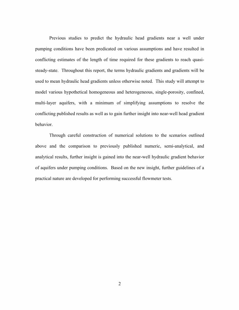
Previous studies to predict the hydraulic head gradients near a well under
pumping conditions have been predicated on various assumptions and have resulted in
conflicting estimates of the length of time required for these gradients to reach quasi-
steady-state. Throughout this report, the terms hydraulic gradients and gradients will be
used to mean hydraulic head gradients unless otherwise noted. This study will attempt to
model various hypothetical homogeneous and heterogeneous, single-porosity, confined,
multi-layer aquifers, with a minimum of simplifying assumptions to resolve the
conflicting published results as well as to gain further insight into near-well head gradient
behavior.
Through careful construction of numerical solutions to the scenarios outlined
above and the comparison to previously published numeric, semi-analytical, and
analytical results, further insight is gained into the near-well hydraulic gradient behavior
of aquifers under pumping conditions. Based on the new insight, further guidelines of a
practical nature are developed for performing successful flowmeter tests.
3
CHAPTER 2
THE USE OF THE ELECTROMAGNETIC BOREHOLE
FLOWMETER FOR MEASURING AND ANALYZING
VERTICAL HYDRAULIC CONDUCTIVITY DISTRIBUTIONS
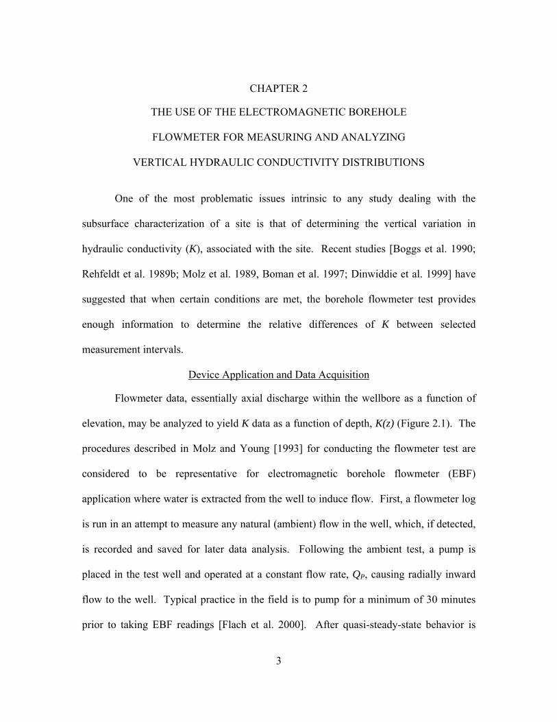
One of the most problematic issues intrinsic to any study dealing with the
subsurface characterization of a site is that of determining the vertical variation in
hydraulic conductivity (K), associated with the site. Recent studies [Boggs et al. 1990;
Rehfeldt et al. 1989b; Molz et al. 1989, Boman et al. 1997; Dinwiddie et al. 1999] have
suggested that when certain conditions are met, the borehole flowmeter test provides
enough information to determine the relative differences of K between selected
measurement intervals.
Device Application and Data Acquisition
Flowmeter data, essentially axial discharge within the wellbore as a function of
elevation, may be analyzed to yield K data as a function of depth, K(z) (Figure 2.1). The
procedures described in Molz and Young [1993] for conducting the flowmeter test are
considered to be representative for electromagnetic borehole flowmeter (EBF)
application where water is extracted from the well to induce flow. First, a flowmeter log
is run in an attempt to measure any natural (ambient) flow in the well, which, if detected,
is recorded and saved for later data analysis. Following the ambient test, a pump is
placed in the test well and operated at a constant flow rate, QP, causing radially inward
flow to the well. Typical practice in the field is to pump for a minimum of 30 minutes
prior to taking EBF readings [Flach et al. 2000]. After quasi-steady-state behavior is
4
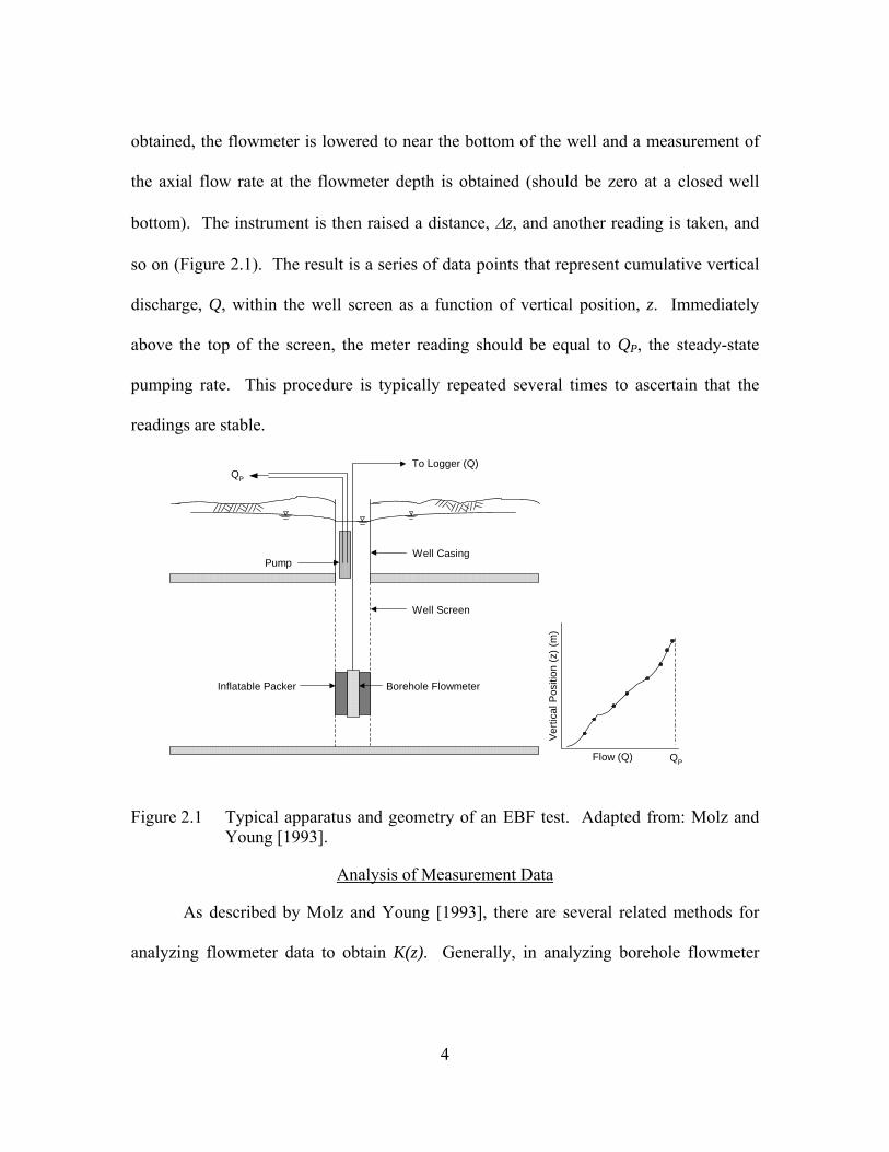
obtained, the flowmeter is lowered to near the bottom of the well and a measurement of
the axial flow rate at the flowmeter depth is obtained (should be zero at a closed well
bottom). The instrument is then raised a distance, Δz, and another reading is taken, and
so on (Figure 2.1). The result is a series of data points that represent cumulative vertical
discharge, Q, within the well screen as a function of vertical position, z. Immediately
above the top of the screen, the meter reading should be equal to QP, the steady-state
pumping rate. This procedure is typically repeated several times to ascertain that the
readings are stable.
To Logger (Q)QP
Pump
Borehole FlowmeterInflatable Packer
Well Screen
Verti
cal P
ositi
on (z
) (m
)
Flow (Q) QP
Well Casing
Figure 2.1 Typical apparatus and geometry of an EBF test. Adapted from: Molz and Young [1993].
Analysis of Measurement Data
As described by Molz and Young [1993], there are several related methods for
analyzing flowmeter data to obtain K(z). Generally, in analyzing borehole flowmeter

5
data, it is assumed that the aquifer is composed of a series of n-horizontal layers (Figure
2.2).
D
z
Q(zi+1):(From Meter)
ΔQi = Q(zi+1) - Q(zi)
z =zi
z = zi+1
DarcyVelocity (v)
ScreenSegment
A=screenArea per Unit
Length=D
Q(zi):(From Meter)
Measurement Intervals
0123
ii+1
n-3n-2n-1 n
Figure 2.2 Idealized aquifer geometry. Adapted from: [Molz and Young 1993].
The differential flow between adjacent layers at given depth, ΔQi, due to pumping
is calculated by taking the difference between two successive meter readings. The
differential ambient flow, Δqi, is calculated in the same manner, if detected. An average
hydraulic conductivity, <K>, for the entire screened section of a well may be calculated
by determining the transmissivity (T) for both a standard pumping test and/or a standard
recovery test using the Cooper-Jacob method [1946]:
( )s
tQbKT P
PUMPING ΔπΔ
××××
=>=<4
log303.2 (2-1)
stt
tQbKT
P
RECOVERY Δπ
Δ
××
⎟⎟⎠
⎞⎜⎜⎝
⎛−
××=>=<
4
log303.21 (2-2)
6
where T is the transmissivity (m2/d), t is time (d), t1 is the duration of pumping (d), s is
the drawdown (m), Δs is the change in head over t1, and b is the aquifer thickness (m).
The flowmeter data are then analyzed using the methods based on a study by
Javandel and Witherspoon [1969], which may be manipulated to yield an equation for
calculating hydraulic conductivity [Molz et al. 1989]:
( )bQ
zqQKK
P
iiii
// ΔΔΔ −
=><
(2-3)
where Ki is the hydraulic conductivity of the ith layer (m/d), <K> is the arithmetic
average hydraulic conductivity (m/d), and Δzi is the thickness of ith layer (m).
Device Design and Theoretical Basis
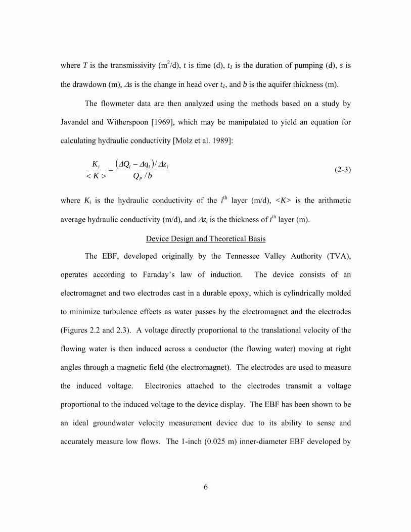
The EBF, developed originally by the Tennessee Valley Authority (TVA),
operates according to Faraday’s law of induction. The device consists of an
electromagnet and two electrodes cast in a durable epoxy, which is cylindrically molded
to minimize turbulence effects as water passes by the electromagnet and the electrodes
(Figures 2.2 and 2.3). A voltage directly proportional to the translational velocity of the
flowing water is then induced across a conductor (the flowing water) moving at right
angles through a magnetic field (the electromagnet). The electrodes are used to measure
the induced voltage. Electronics attached to the electrodes transmit a voltage
proportional to the induced voltage to the device display. The EBF has been shown to be
an ideal groundwater velocity measurement device due to its ability to sense and
accurately measure low flows. The 1-inch (0.025 m) inner-diameter EBF developed by
7
the TVA and manufactured by the Quantum Engineering Corporation is sensitive to
flows ranging from 40 mL/min to 40 L/min (0.05 m3/d to 57.6 m3/d) [Waldrop 1995].
Figure 2.3 Schematic diagram of the EBF [Molz and Young 1993].
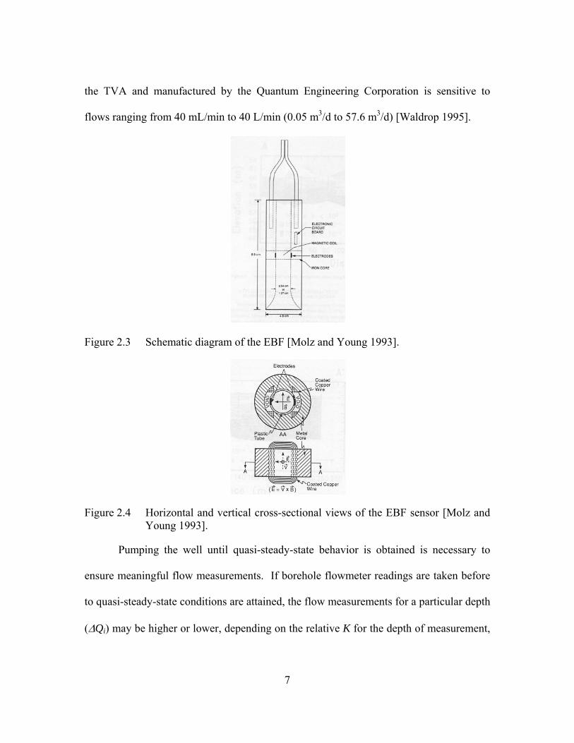
Figure 2.4 Horizontal and vertical cross-sectional views of the EBF sensor [Molz and Young 1993].
Pumping the well until quasi-steady-state behavior is obtained is necessary to
ensure meaningful flow measurements. If borehole flowmeter readings are taken before
to quasi-steady-state conditions are attained, the flow measurements for a particular depth
(ΔQi) may be higher or lower, depending on the relative K for the depth of measurement,
8
than the quasi-steady-state flow for that depth due to cross-flow between layers resulting
from vertical hydraulic gradients. This deviation of ΔQi during transient conditions in
turn results in calculated K values that deviate from their “true” value. The magnitude
and behavior of the deviations, however, are not clear at the present time. Whereas the
details of applying the EBF and accounting for the possible errors as well as the post-test
analysis of the data having been discussed in detail [Molz and Young 1993; Kabala 1994;
Ruud and Kabala 1996; Boman et al. 1997; Young 1998; Dinwiddie et al. 1999; Ruud et
al. 1999; Arnold and Molz 2000], the final questions left to be answered definitively is
how long of a pumping interval is required for a system to attain quasi-steady-state
conditions and how close to such conditions must one be to obtain K values that are
useful in a practical sense.
To estimate the time required for the flows at the well to reach quasi-steady-state,
some a priori knowledge of the geological profile of the well is required. This
knowledge will typically consist of the boring log recorded at the time of the well
installation. Using this information, a model may be constructed to estimate the
hydraulic behavior over the depth of the borehole or the length of the well screen. The
model may then be used to predict the hydraulic gradient for each layer as a function of
time. As these gradients cease to change “appreciably”, the flow out of each layer will
cease to change “appreciably” and the aquifer is considered to have reached “practical”
quasi-steady-state. In most applications, it is more important to accurately identify high-
K layers than low-K layers. Thus, information on how such layers behave in the vicinity
of quasi-steady-state is important also.

9
CHAPTER 3
GENERAL THEORY OF VERTICALLY STRATIFIED
AQUIFERS
There exists, in general, two ways to characterize vertically stratified aquifers: 1)
as systems where there is no connection, or water flow, between the layers (Figure 3.1),
or 2) as systems where crossflow between the layers occurs (Figure 3.2). Of these two
cases, the allowance for crossflow between layers is more realistic physically; however, it
is more complex to evaluate. The actual amount and behavior of crossflow that a system
experiences will be a function of time, the vertical to horizontal K ratio, or anisotropy,
and the differential horizontal K (or more specifically, differences in the ratio of
horizontal K and specific storage, or hydraulic diffusivity) between adjacent layers. The
amount of crossflow occurring between layers at any given time prior to quasi-steady-
state (please see Chapter 1 for a definition of quasi-steady-state) affects the behavior of
the hydraulic gradients for each layer. Once quasi-steady-state is approached in the
vicinity of the well, the hydraulic gradients at the well face are essentially equal and
constant and crossflow becomes negligible.
10
Well Face
K=300 m/d
K=1000 m/d
K=30 m/d
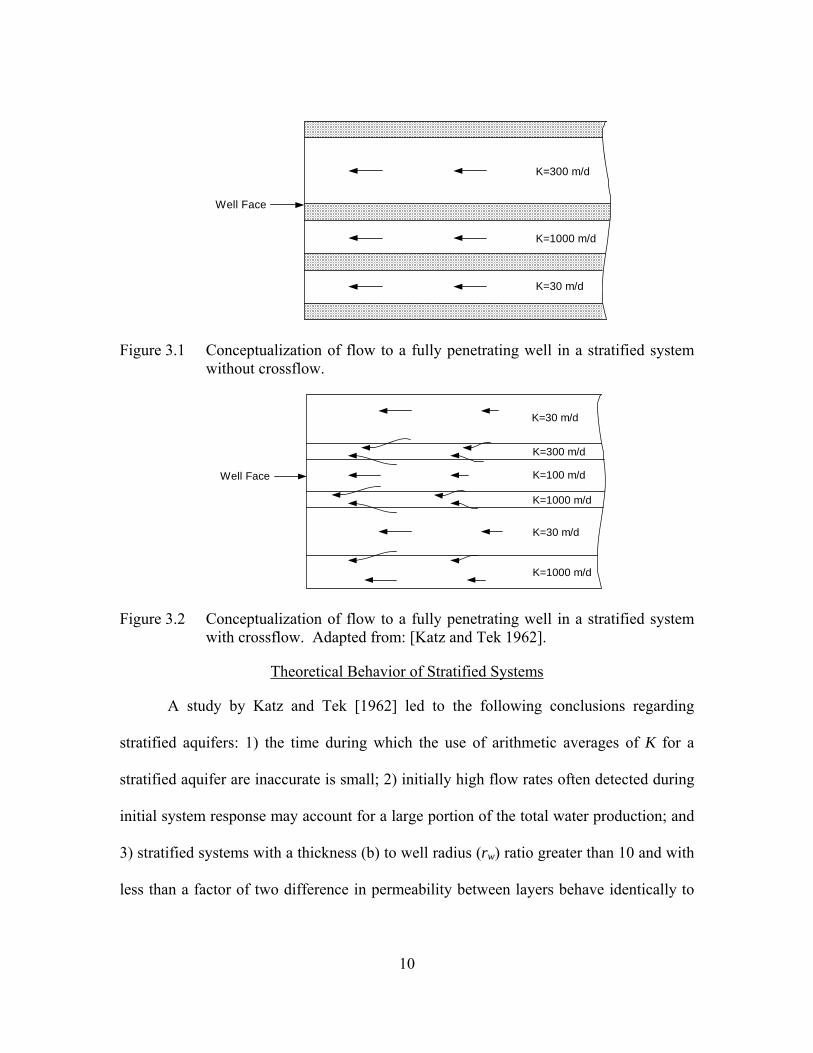
Figure 3.1 Conceptualization of flow to a fully penetrating well in a stratified system without crossflow.
Well Face
K=30 m/d
K=300 m/d
K=100 m/d
K=1000 m/d
K=30 m/d
K=1000 m/d
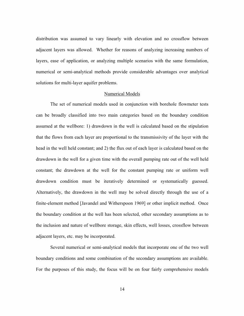
Figure 3.2 Conceptualization of flow to a fully penetrating well in a stratified system with crossflow. Adapted from: [Katz and Tek 1962].
Theoretical Behavior of Stratified Systems
A study by Katz and Tek [1962] led to the following conclusions regarding
stratified aquifers: 1) the time during which the use of arithmetic averages of K for a
stratified aquifer are inaccurate is small; 2) initially high flow rates often detected during
initial system response may account for a large portion of the total water production; and
3) stratified systems with a thickness (b) to well radius (rw) ratio greater than 10 and with
less than a factor of two difference in permeability between layers behave identically to

11
single layer systems constructed using an arithmetic mean permeability of the layered
system. The second finding was confirmed by Russell and Prats [1962], who found that
an exponential rate decline in production occurs rapidly. Russell and Prats [1962]
showed, that for a two-layer system, the time to reach the exponential decline in
production could be approximated by:
( )( ) 3.02 ≈
effTOTAL
TOTAL
rchtkh
μθ (3.1)
where k is the permeability, h is the thickness of a given layer, c is the coefficient of
compressibility for water, μ is the water viscosity, and TOTAL denotes the property total
(i.e., (Kh)TOTAL for a two-layer system equals k1h1+k2k2).
Factors Influencing Crossflow
As a vertically stratified aquifer undergoes pumping, the higher-K layers will
initially account for the majority of the system water yield. As the higher-K layers begin
to deplete water from storage, a vertical head gradient between the higher-K layers and
the lower-K layers is induced and the water in the lower-K layers begins to respond to the
change in vertical head gradient by flowing into the higher-K layers. This movement of
water from one layer to another, or crossflow, will continue until the difference in
hydraulic head between layers becomes zero. When crossflow becomes negligible, the
system will be near quasi-steady-state. This implies that the hydraulic head gradients at
the well face are constant and equal and flow to the well is constant, uniform, and
horizontal.

12
It is possible to place upper and lower bounds on the amount of crossflow a given
system may experience by considering the limiting cases. The lower bound for crossflow
is the case where the producing layers are isolated from each other by impermeable layers
(Figure 3.1). The upper bound for crossflow is the situation where the lower-K layers are
able to indefinitely supply water to the higher-K layers and where flow between the lower
and higher-K layers is instantaneous (i.e., infinite vertical K) [Katz and Tek 1962].
Whereas it may be possible, due to large differences in K between layers, to reliably and
accurately portray an aquifer as a series of sub-aquifers separated by confining units
(Figure 3.1), it is less probable that an aquifer may be represented using an infinite
vertical K. It should be noted, however, that vertical wells often behave in a manner
consistent with an infinite vertical K [Elci et al. 2001]. Katz and Tek [1962] proposed
that the effect of vertical K on crossflow is related to the relative thickness of the system
compared to the system extents; i.e., decreasing the thickness of the system will have the
same effect as increasing the vertical K. In general, as the measured vertical
heterogeneity resolution is increased, it becomes less feasible to approximate a system
according to either limiting scenario. For this reason, it is important to understand the
factors that influence the degree of crossflow in a system at a given place and time.

13
CHAPTER 4
COMPARISON OF DIFFERENT METHODS FOR MODELING
HYDRAULIC GRADIENT OR DRAWDOWN BEHAVIOR IN
VERTICALY STRATIFIED CONFINED AQUIFERS
Analytical Models
Numerous researchers have presented analytical models to solve for the flows in
multi-layer aquifer systems. Generally, these solutions are highly complex and any
advantage they may have due to the exactness of the solution is far outweighed by their
impracticality in terms of evaluation and inflexibility with respect to the assumptions and
conditions that must be satisfied for the solution(s) to be applicable. Katz and Tek [1962]
and Russell and Prats [1962] developed analytical models that provided solutions for
bounded two-layer aquifers with crossflow and a constant drawdown at the wellbore.
Jacquard [1960] presented an analytical solution for a similar system but with a constant
pumping rate. Several other analytical solutions for two-layer systems allow for partially
penetrating wells where the well is located in only one of the two layers [Javandel and
Witherspoon 1980; Javandel and Witherspoon 1983; Szekely 1995]. The vast majority of
remaining analytical models for multi-layer aquifer systems can be more accurately
described as multi-aquifer solutions, as they are only applicable for multiple aquifer units
separated by aquitards (Figure 3.1). The analytical solutions provided by Neuman and
Witherspoon [1969], Hemker [1985], Hunt [1985], Maas [1987], and Hemker and Maas
[1987] all fall into this category. In 1989, Sen [1989] presented an analytical solution for
the case of a vertically graded aquifer where the vertical hydraulic conductivity
14
distribution was assumed to vary linearly with elevation and no crossflow between
adjacent layers was allowed. Whether for reasons of analyzing increasing numbers of
layers, ease of application, or analyzing multiple scenarios with the same formulation,
numerical or semi-analytical methods provide considerable advantages over analytical
solutions for multi-layer aquifer problems.
Numerical Models
The set of numerical models used in conjunction with borehole flowmeter tests
can be broadly classified into two main categories based on the boundary condition
assumed at the wellbore: 1) drawdown in the well is calculated based on the stipulation
that the flows from each layer are proportional to the transmissivity of the layer with the
head in the well held constant; and 2) the flux out of each layer is calculated based on the
drawdown in the well for a given time with the overall pumping rate out of the well held
constant; the drawdown at the well for the constant pumping rate or uniform well
drawdown condition must be iteratively determined or systematically guessed.
Alternatively, the drawdown in the well may be solved directly through the use of a
finite-element method [Javandel and Witherspoon 1969] or other implicit method. Once
the boundary condition at the well has been selected, other secondary assumptions as to
the inclusion and nature of wellbore storage, skin effects, well losses, crossflow between
adjacent layers, etc. may be incorporated.
Several numerical or semi-analytical models that incorporate one of the two well
boundary conditions and some combination of the secondary assumptions are available.
For the purposes of this study, the focus will be on four fairly comprehensive models
15
constructed specifically to analyze multi-layer aquifers which have undergone validation
and have been compared to at least one other model of the four: Javandel and
Witherspoon [1969], Ruud and Kabala [1996, 1997], Hemker [1999a, 1999b], and
Kabala and El-Sayegh [2002].
Javandel and Witherspoon [1969]
One of the earliest comprehensive numerical solutions was set forth by Javandel
and Witherspoon [1969] for a two-layer confined aquifer with a single pumping well.
The numerical code constructed by Javandel and Witherspoon [1969] is a finite element
model formulated to solve transient fluid flow in heterogeneous, two-layer and multi-
layer, isotropic and anisotropic aquifers. Both constant rate pumping and constant head
boundaries are permitted boundary conditions at the well, no flow boundaries are
imposed on the top and bottom of the aquifer, and a constant head boundary is assumed
to exist far from the production well. Crossflow between the different layers is allowed.
The results from the Javandel and Witherspoon [1969] study revealed four key findings.
First, at early times the gradient behaviors in layers with different K are significantly
different due to preferential flow in the higher-K layer(s). This difference diminishes
with time as the flows in the layers equilibrate and the drawdown in each layer
approaches the Theis solution: the smaller the difference in K values between the layers,
the shorter the time frame for convergence to the Theis solution, due to decreasing
amounts of crossflow between layers. Second, after the first few minutes of pumping, the
differences between the near-well drawdown in the layers and the Theis solution are
negligible. Javandel and Witherspoon [1969] note, however, this may not be true away

16
from the wellbore or in thick, multi-layer aquifers. Third, deviations from the Theis
solution in a given layer are less for those layers with higher-K values. Finally, once the
system has attained a quasi-steady-state condition, implying that flow is constant and
horizontal out of each layer, the flux from each layer into the well is proportional to the K
of the layer.
Ruud and Kabala [1996]
In 1996, Ruud and Kabala proposed a numerical model for simulating the near-
well hydraulic behavior of layered confined aquifers under pumping conditions. The
model was constructed to determine the non-uniform wellbore flux distribution for a fully
penetrating well. The model is a fully implicit finite difference approximation subject to
no flow boundaries at the top and bottom of the aquifer, no drawdown at the effective
radius boundary, and the pumping condition (also referred to as the well constraint
boundary) at the wellbore. The results of Ruud and Kabala’s modeling efforts suggest
that, contrary to the results of Javandel and Witherspoon [1969], the flux along the
wellbore for some layers may be persistently transient or non-uniform. For the parameter
values studied, the Javandel and Witherspoon [1969] analysis showed that flows toward a
well in layered aquifers quickly become horizontal. In certain cases, therefore, the Ruud
and Kabala [1996] model findings deviate from the Javandel and Witherspoon [1969]
model findings. The situations in which the conclusions differ are those aquifers having
low hydraulic conductivity and high storativity (i.e., low hydraulic diffusivity), which
was not considered in detail by Javandel and Witherspoon [1969]. They also pointed out
correctly that the hydraulic diffusivity ratio between adjacent layers, rather than the

17
magnitude of the corresponding K ratio, is the appropriate parameter for analyzing multi-
layer aquifers and flowmeter tests.
Hemker [1999a, 1999b]
Hemker’s [1999a, 1999b] model for analyzing flow behavior to a well in layered
aquifers is a hybrid analytical-numerical model where the radial component is solved
analytically and the vertical component is solved numerically. The model was originally
constructed to study changes in specific storage (Ss) under pumping conditions. The
mathematical formulation for the model is essentially the same as that used by Ruud and
Kabala [1997] with obvious changes made to allow for the analytical-numerical solution
scheme. The constant head model [1999a], which assumes that the flow into the well
from each layer is proportional to the layer transmissivity, allows for ready comparison to
the majority of other analytical and numerical models available for modeling layered
systems; however, even in homogeneous systems this assumption of a constant head in
the well or uniform wellbore flux is not generally correct. Hemker [1999b] suggested
using a uniform drawdown at the well boundary (i.e., the flow into the well from each
layer is not necessarily proportional to the layer transmissivity prior to steady-state) as a
more realistic boundary condition. This type of boundary condition greatly complicates
the solution of the model due to the need for iteration in solving the fluxes from each
layer such that they satisfy the boundary condition. Hemker [199b] acknowledges that
the drawdown in the well could alternatively be solved directly using the principle of
superposition [Javandel and Witherspoon 1969] or other simultaneous solution
techniques. Hemker’s results [1999b] largely focus on scenarios with partially-

18
penetrating wells in confined aquifers, with scenarios focusing on fully-penetrating wells
in confined aquifers discussed to a lesser extent. With respect to fully-penetrating wells
in confined aquifers, Hemker [1999b] found that at early times, the two well boundary
conditions (constant head versus uniform drawdown) resulted in drawdowns at the well
that differed by as much as 27% and that this difference gradually decreases with time.
Hemker [1999b] also reported that the system exhibited vertical gradients in the layers
until 0.1 days (2.4 hours).
Kabala and El-Sayegh [2002]
Kabala and El-Sayegh [2002] have assembled a fairly comprehensive review of
the transient flowmeter test models including no crossflow models, numerical crossflow
models, semi-analytical crossflow models with no skin, semi-analytical crossflow models
with infinitesimal skin, and semi-analytical crossflow models with thick skin, in addition
to their own model which is a semi-analytical model that accounts for uniformly thick
skin, wellbore storage, and crossflow. Like the Javandel and Witherspoon [1969] model,
the Kabala and El-Sayegh [2002] model is constructed using the constant head boundary.
The Kabala and El-Sayegh [2002] model also uses an approximation of transient
crossflow characterized by the differential quotient of layer-averaged drawdowns in
adjacent layers. The Kabala and El-Sayegh [2002] model was compared to the Ruud and
Kabala [1996, 1997] model, which relaxes the uniform wellbore flux and pseudo-steady-
state crossflow assumptions. Kabala and El-Sayegh [2002] concluded that their model
compared favorably with the Ruud and Kabala [1996, 1997] model for the scenarios
tested. In addition, Kabala and El-Sayegh [2002] concluded that their model was capable

19
of interpreting multiple pumping rate transient flowmeter tests so long as the proper
Laplace transform inversion algorithm is used, such as the De Hoog et al. inversion [De
Hoog et al. 1982].
Summary of Selected Models
Of the four models discussed, only the Javandel and Witherspoon [1969] and
Ruud and Kabala [1996, 1997] models deal specifically and rigorously with the
assessment of individual layer hydraulic gradient behavior. The Javandel and
Witherspoon [1969] model resulted in short times to hydraulic gradient quasi-steady-state
and postulated that from a practical standpoint, deviations from the Theis solution were
negligible after a dimensionless time of 1,000 (see Chapter 5 for the definition of
dimensionless time), which was generally on the order of several minutes. Ruud and
Kabala [1996, 1997] found that for some systems, or some layers within certain systems,
reaching quasi-steady-state could require a significantly long time. For example, the
layer flows for a two-layer system with K-values of 4.0E-05 m/s and 4.0E-07 m/s and
with Ss-values of 1.0E-05 and 1.0E-03 m-1 had not reached quasi-steady-state at three
hours or a dimensionless time of nearly 29,000 (calculated in the same manner as
Javandel and Witherspoon [1969]. The Hemker [1999b] model examined layer-specific
behavior as a function of cumulative flow and behavior radially distant from the well, but
made little mention of the transient behavior of individual layer hydraulic head gradients.
The single scenario consisting of a fully-penetrating well in a confined, heterogeneous
aquifer reported by Hemker [1999b] was reported to attain quasi-steady-state in 2.4
hours. The Kabala and El-Sayegh [2002] model was constructed specifically to analyze
20
multiple pumping rate transient flowmeter tests, which does not require quasi-steady-
state conditions. Kabala and El-Sayegh [2002] do note however, that whereas their model
results compares well to the Ruud and Kabala [1996, 1997] model results, errors for the
Kabala and El-Sayegh [2002] model increase as the hydraulic diffusivity contrast
increases.
The challenge presented through the comparison of these four models is to create
an independent model capable of:
1. accurately and reliably reproducing their bulk results;
2. addressing the smaller inconsistencies between them; and
3. providing meaningful and conclusive data regarding the hydraulic gradient
behavior for layered systems.
This report will discuss the influences of key parameters on the hydraulic gradient
response including:
• layer hydraulic conductivity;
• layer specific storage;
• layer thickness;
• layer arrangement; and
• overall system thickness.
In addition, the following inconsistencies in the literature conclusions will be addressed
and resolved, especially the conflicting statements of the time required to attain quasi-
steady-state from Javandel and Witherspoon [1969] and Ruud and Kabala [1997].

21
Finally, the potential implications of the common practice of pumping for 30 minutes
prior to taking EBF readings with respect to the values of K obtained is discussed.
22
CHAPTER 5
HYDRAULIC GRADIENT BEHAVIOR IN SINGLE-DOMAIN,
MULTI-LAYER CONFINED AQUIFERS WITH
HOMOGENEOUS AND ISOTROPIC OR ANISOTROPIC
LAYERS
Physical Model
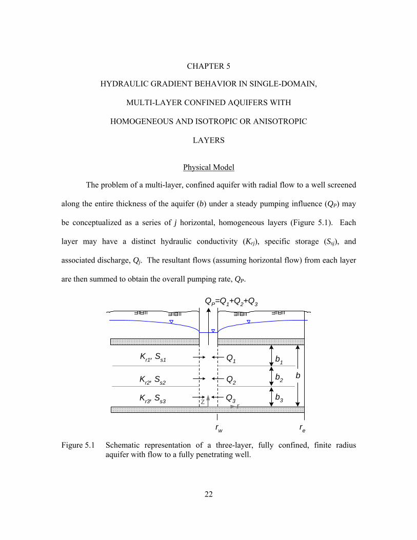
The problem of a multi-layer, confined aquifer with radial flow to a well screened
along the entire thickness of the aquifer (b) under a steady pumping influence (QP) may
be conceptualized as a series of j horizontal, homogeneous layers (Figure 5.1). Each
layer may have a distinct hydraulic conductivity (Krj), specific storage (Ssj), and
associated discharge, Qj. The resultant flows (assuming horizontal flow) from each layer
are then summed to obtain the overall pumping rate, QP.
QP=Q1+Q2+Q3
Q2bb2
b1
Kr2, Ss2
Q1Kr1, Ss1
z r
rw re
Kr3, Ss3 Q3 b3
Figure 5.1 Schematic representation of a three-layer, fully confined, finite radius
aquifer with flow to a fully penetrating well.
23
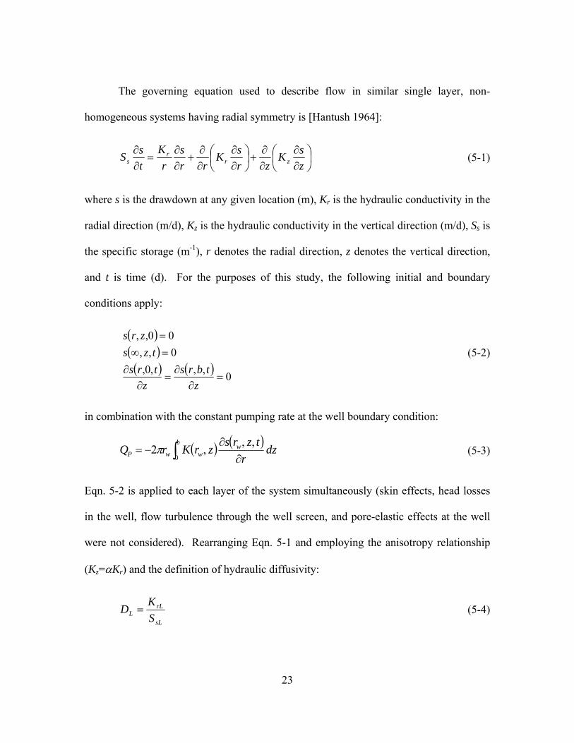
The governing equation used to describe flow in similar single layer, non-
homogeneous systems having radial symmetry is [Hantush 1964]:
⎟⎠⎞
⎜⎝⎛
∂∂
∂∂
+⎟⎠⎞
⎜⎝⎛
∂∂
∂∂
+∂∂
=∂∂
zsK
zrsK
rrs
rK
tsS zr
rs (5-1)
where s is the drawdown at any given location (m), Kr is the hydraulic conductivity in the
radial direction (m/d), Kz is the hydraulic conductivity in the vertical direction (m/d), Ss is
the specific storage (m-1), r denotes the radial direction, z denotes the vertical direction,
and t is time (d). For the purposes of this study, the following initial and boundary
conditions apply:
( )( )
( ) ( ) 0,,,0,0,,00,,
=∂
∂=
∂∂
=∞=
ztbrs
ztrstzs
zrs (5-2)
in combination with the constant pumping rate at the well boundary condition:
( ) ( ) dzr
tzrszrKrQ wb
wwP ∂∂
−= ∫,,,2
0π (5-3)
Eqn. 5-2 is applied to each layer of the system simultaneously (skin effects, head losses
in the well, flow turbulence through the well screen, and pore-elastic effects at the well
were not considered). Rearranging Eqn. 5-1 and employing the anisotropy relationship
(Kz=αKr) and the definition of hydraulic diffusivity:
sL
rLL S
KD = (5-4)

24
where L is the layer designation, yields:
2
2
2
211zs
rs
rs
rts
DLLLL
L ∂∂
+∂∂
+∂∂
=∂
∂α (5-5)
Similarly, the boundary conditions are extended to the multi-layer problem:
( )( )
( ) ( )0
,,,0,0,,00,,
=∂
∂=
∂∂
==
ztbrs
ztrstzrs
zrs
LL
eL
L
(5-6)
with the constant pumping rate at the well boundary condition:
( )r
tzrsbKrQ wL
n
LLrLwP ∂
∂−= ∑
=
,,2
1
π (5-7)
Steady-State Derivation
The steady-state relationship for a single-layer, confined aquifer with a finite
effective radius may be obtained from Eqn. 5-1, combined with the pumping condition at
the well (Eqn. 5-7) and the other boundary conditions (Eqn. 5-6).
2
2
2
2
0z
sKr
sKrs
rK
zrr
∂∂
+∂∂
+∂∂
= (5-8)
At steady-state, we can further assume that all flow is horizontal, such that the vertical
term goes to zero. As Kr is considered to be uniform, we may drop that coefficient and
we are left with the following:
2
210dr
sddrds
r+= (5-9)
25
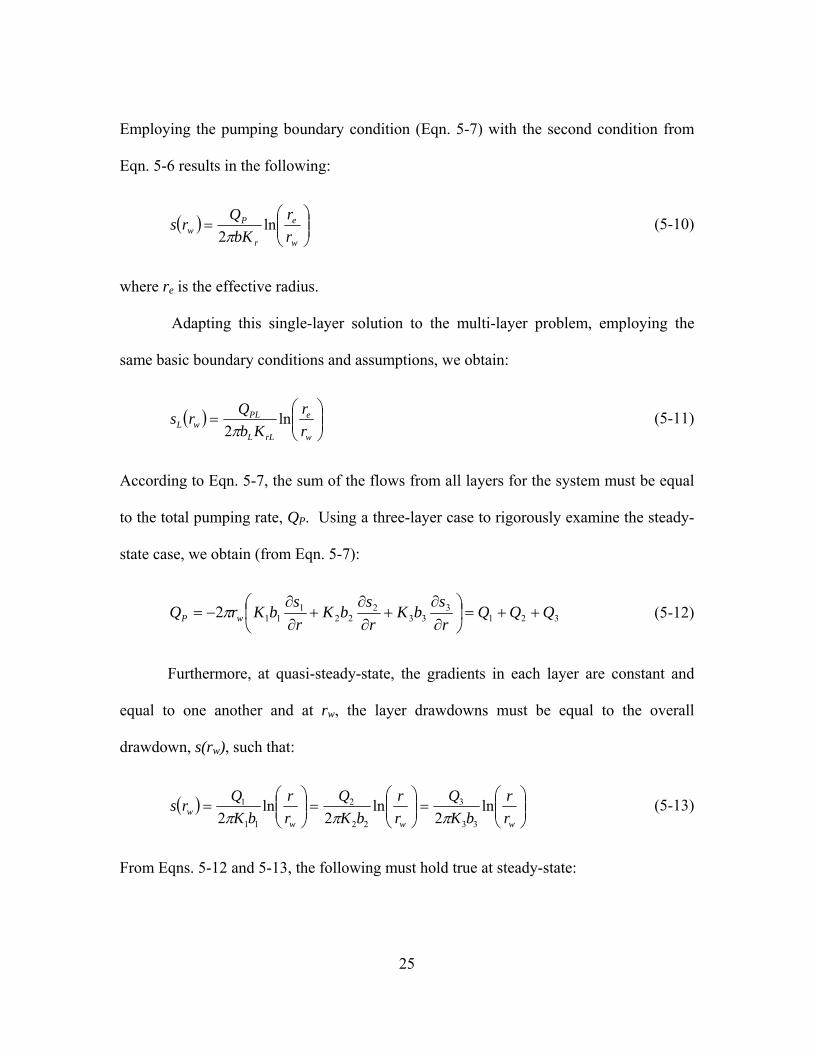
Employing the pumping boundary condition (Eqn. 5-7) with the second condition from
Eqn. 5-6 results in the following:
( ) ⎟⎟⎠
⎞⎜⎜⎝
⎛=
w
e
r
Pw r
rbK
Qrs ln2π
(5-10)
where re is the effective radius.
Adapting this single-layer solution to the multi-layer problem, employing the
same basic boundary conditions and assumptions, we obtain:
( ) ⎟⎟⎠
⎞⎜⎜⎝
⎛=
w
e
rLL
PLwL r
rKb
Qrs ln2π
(5-11)
According to Eqn. 5-7, the sum of the flows from all layers for the system must be equal
to the total pumping rate, QP. Using a three-layer case to rigorously examine the steady-
state case, we obtain (from Eqn. 5-7):
3213
332
221
112 QQQrs
bKrs
bKrs
bKrQ wP ++=⎟⎠⎞
⎜⎝⎛
∂∂
+∂∂
+∂∂
−= π (5-12)
Furthermore, at quasi-steady-state, the gradients in each layer are constant and
equal to one another and at rw, the layer drawdowns must be equal to the overall
drawdown, s(rw), such that:
( ) ⎟⎟⎠
⎞⎜⎜⎝
⎛=⎟⎟
⎠
⎞⎜⎜⎝
⎛=⎟⎟
⎠
⎞⎜⎜⎝
⎛=
wwww r
rbK
Qrr
bKQ
rr
bKQrs ln
2ln
2ln
2 33
3
22
2
11
1
πππ (5-13)
From Eqns. 5-12 and 5-13, the following must hold true at steady-state:
26
( ) 33
3
22
2
11
1
332211 bKQ
bKQ
bKQ
bKbKbKQP ===
++ (5-14)
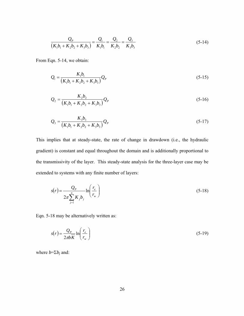
From Eqn. 5-14, we obtain:
( ) PQbKbKbK
bKQ332211
111 ++
= (5-15)
( ) PQbKbKbK
bKQ
332211
222 ++
= (5-16)
( ) PQbKbKbK
bKQ
332211
333 ++
= (5-17)
This implies that at steady-state, the rate of change in drawdown (i.e., the hydraulic
gradient) is constant and equal throughout the domain and is additionally proportional to
the transmissivity of the layer. This steady-state analysis for the three-layer case may be
extended to systems with any finite number of layers:
( ) ⎟⎟⎠
⎞⎜⎜⎝
⎛=
∑=
w
en
jjj
P
rr
bK
Qrs ln
21
π (5-18)
Eqn. 5-18 may be alternatively written as:
( ) ⎟⎟⎠
⎞⎜⎜⎝
⎛=
w
eP
rr
KbQ
rs ln2π
(5-19)
where b=Σbj and:

27
∑
∑
=
== n
jj
n
jjj
b
bKK
1
1 (5-20)
Numerical Model
TMVOC [Pruess and Battistelli 2002], a specialized module of the TOUGH2
simulator [Pruess et al. 1999], was employed throughout this study to simulate different
aquifer scenarios. TMVOC was developed primarily to analyze non-aqueous phase
liquid (NAPL) fate and transport for both unsaturated and saturated subsurface
conditions. By selecting for certain modules and by properly parameterizing select
variables, it is possible to employ TMVOC to analyze the single-phase (i.e., water),
confined aquifer flow to a well under a constant pumping rate. TMVOC was selected for
this study based on its ability to solve radial domain scenarios as well as its being an
integral finite difference model (IFDM) which allows for the direct solution of drawdown
in a well for a multi-layer aquifer system subject to pumping. A robust body of literature
about and using the TOUGH2 and TMVOC simulators exists, including verification and
validation of the models [Moridis and Pruess 1995; Pruess et al. 1996]. As the TMVOC
simulator has been previously verified and validated by the developers and other
researchers, these steps are not repeated herein; however, testing of the simulator for
special cases was performed by comparing the model results to several analytical
solutions to ensure proper use of the simulator in this application.
28
Model Space and Time Discretization
The mass and energy balance equations solved by the TOUGH2 family of codes
may be expressed as [Finsterle et al. 2006; Pruess and Battistelli 2002]:
∫ ∫ ∫Γ
+Γ•=n n nV V
nnn dVqndFdVMdtd κκκ (5-22)
where the integration is performed over the subdomain Vn, which is bounded by the
surface Γn; M represents mass, with κ representing the mass component (i.e., water); F
represents mass flux; q represents sinks or sources; and n is the unit normal vector on
surface element dΓn, pointing inward into Vn. The mass accumulation term for water is
[Finsterle et al. 2006]:
∑=β
κβββ
κ ρφ xSM (5-23)
where β is the phase, φ is porosity, Sβ is the saturation of phase β, ρβ is the density of
phase β, and xβκ is the mass fraction of component κ in phase β (in the TMVOC version
of the TOUGH code, this is a molar fraction). The advective mass flux is summed over
phases [Finsterle et al. 2006]:
∑=β
βκβ
κ FxFadv
(5-24)
Applying Darcy’s law yields [Pruess and Battistelli 2002]:
( )gPk
kuF rββ
β
βββββ ρ
μρ
ρ −∇−== (5-25)
29
where uβ is the Darcy velocity in phase β, k is absolute permeability, krβ is relative
permeability of phase β (since this study involves the single phase flow of water, krβ is
equal to 1), μβ is viscosity, and
ββ cPPP += (5-26)
where Pβ is the pressure in phase β, P is the reference pressure, and Pcβ is the capillary
pressure (zero for single phase). Eqn. 5-22 can be discretized in time and space using the
IFDM method, using appropriate volume averages, to obtain [Pruess and Battistelli
2002]:
nnV
n MVdVMn
∫ =κ (5-27)
∫ ∑Γ
=Γ•n
mnmnmn FAndF κ (5-28)
Where Fnm is the average value of the normal component of F over the surface Anm
between volume elements Vn and Vm. For the Darcy flux term [Pruess and Battistelli
2002]:
⎥⎦
⎤⎢⎣
⎡−
−
⎥⎥⎦
⎤
⎢⎢⎣
⎡−= nmnm
nm
mn
nm
rnmnm g
DPPk
kF ,,,
, βββ
β
βββ ρ
μρ
(5-29)
where nm denotes the interface between blocks n and m, Dnm is the distance between the
nodal points n and m, and gnm is the component of gravitational acceleration from m to n.

30
Numerical Model Application
Verification of the numeric model was conducted by comparing the numeric
model results to: 1) the steady-state solution for a homogeneous, isotropic, fully-
confined, fully-penetrating well, finite-radius system [Thiem 1906]; and 2) transient
solutions for a homogeneous, isotropic, fully-confined, fully-penetrating well, infinite-
radius system [Hantush 1964; Theis 1935; Lee 1998]. It should be noted that the
analytical time-domain solutions assume the aquifer to be infinite in horizontal extent;
however, these solutions may be compared to the finite numerical case until the far radial
boundary begins to influence the system behavior. Once steady-state for the finite-radius
system is attained the transient analytical solutions are no longer comparable. To ensure
that the assumptions of the analytical infinite domain solutions may be comparable over a
significant range of time, a sufficiently large effective radius is employed in the
numerical model.
Equivalency of the IFDM to the FDM
The mass and energy balance equations solved by the TOUGH2 family of codes can be
related to the parameters typically evaluated in single-phase groundwater flow (e.g., head
or drawdown, hydraulic diffusivity (hydraulic conductivity and specific storage), flow,
etc.). Substituting Eqns. 5-24 and 5-25 into Eqn. 5-22 results in [Pruess and Battistelli
2002]:
∑ +=m
nmnmn
n qFAVdt
dM κκκ 1 (5-30)
For single-phase groundwater flow [Finsterle et al. 2006],
31
dtdh
Sdt
dM ns
nβ
κ
ρ= (5-31)
where Ss is specific storage and h is the hydraulic head in element n. Other terms are
defined as:
wwM φρ= (5-32)
β
β
μρ g
kK nmnm = (5-33)
zg
Ph ∇+
∇=∇
β
β
ρ (5-34)
where Knm is the hydraulic conductivity of phase β. Changes in hydraulic head, h, can be
related to drawdown, s, as follows:
dhds −= (5-35)
Eqns. 5-28 through 5-30 can be substituted into Eqns. 5-26 and 5-27 to obtain:
( )∑ +∇−=m nm
nm
n
qsDA
Vdtds
D11
(5-36)
Eqn. 5-36 demonstrates that as with Eqn. 5-5, the IDFM system of equations can be
simplified such that the hydraulic diffusivity, D, and the sum of Δz, or the aquifer
thickness (b) are the sole variables that differ between simulations (assuming that the
radial domain is held constant across all model scenarios).

32
Numerical Model Set-up
Universal Parameters
Universal parameters are those which were determined prior to beginning
modeling and which are held constant across all simulations. These parameters include:
• Temperature – 20 degrees Celsius; the temperature of the system was
selected such that the viscosity of water is 1 centipoise (cp).
• Water compressibility (β) – 4.4E-10 Pa-1.
• Water density (ρ) – 998.2 kg/m3, the density of water at 20 degrees
Celsius.
• Porosity (φ) of the well elements – 0.99. In real-world applications, the
porosity inside the well would be considered to be 1.0; 0.99 was employed
to avoid instability in the model.
• Well parameters:
o Permeability (k) of the well elements – Sinks and sources (water in
this study) are handled through the GENER module in TMVOC,
where a production (<0) or generation rate (>0) is defined and
applied to the elements specified. The extraction rate (production
rate) is specified within in the GENER module to be a constant
mass rate throughout each simulation. The elements where the
production or generation rate is applied must also be defined in the
ROCKS module. To simulate an open well with negligible losses,
the permeability of the elements making up the interior of the well

33
should be assigned a k greater than any applied within the aquifer
elements. For this study, the k was initially set to 1.0E-07 m2 and
was incrementally increased until the differences between
successive model run drawdowns were no longer changing. The
extraction rate (production rate) is then applied to the bottom-most
well element to simulate water extraction.
o Well Radius (rw) – set to 0.05 m (or 4 in, a typical flowmeter test
well diameter).
o Effective Radius (re) – set to 20,000 m to avoid boundary effects
during the time-frame of interest (i.e., early time or time prior to
steady-state).
Variable Definitions
There are several variables must be defined for each simulation or calculated
based on defined parameters:
• Porosity (φ) – porosity is set for each material defined in ROCKS using
typical values for the materials being considered in each simulation. For
instance, φ is set to 0.35 for medium sands.
• Pore compressibility (COM) – The pore compressibility must be defined
for each material defined in the ROCKS module and is a function of the
layer specific Storage (Ss):
βϕρ
−=gSCOM s (5-37)

34
where g is the acceleration of gravity (9.81 m/s2). Storage may be defined
as the following:
th
hM
tM
∂∂
∂∂
=∂
∂
(5-38)
where dM/dH is the storage coefficient. Using Eqns. 5-32 and 5-38, the
following is obtained:
( )hh
M∂
∂=
∂∂ φρ
(5-39)
Using the product rule on the right-hand term yields:
( )hhh ∂
∂+
∂∂
=∂
∂ ρφφρφρ
(5-40)
where the first portion of the right-hand term represents aquifer
compression and the second portion represents water compression. The
density of a slightly compressible liquid, such as water, may be defined as:
( ){ }olo PP −= βρρ exp (5-41)
where r=ro at P=Po and βl is the compressibility of water (4.4E-10 Pa-1).
Again, using the chain rule:
hP
Ph ∂∂
∂∂
=∂∂ ρρ
(5-42)
where:
gzghP ρρ += (5-43)
35
such that:
ghP ρ=
∂∂
(5-44)
Then, using Eqn. 5-41, the following is obtained:
( ){ } ρββρβρlolol PP
P=−=
∂∂ exp (5-45)
which may be rearranged to obtain:
Pl ∂∂
=ρ
ρβ 1
(5-46)
The combination of Eqns. 5-41 though 5-46 yields:
lgP
gh
βφρρρϕρρφ )(=∂∂
=∂∂
(5-47)
Now, for aquifer compression,
Pg
hP
Ph ∂∂
=∂∂
∂∂
=∂∂ φρφφ
(5-48)
From soil mechanics, the compressibility of soil may be defined as:
'1
σ∂∂−
= T
Tb
VV
C (5-49)
Where Cb is compressibility, VT is total volume, and σ’ is effective stress.
If it is assumed that the change in total volume is the sum of the change in
void volume (VV) and the change in solids volume (VS) and additionally

36
that the change in VS is much less than the change in VV such that dVT is
approximately equal to dVV. Furthermore, VV=φVT. This results in:
( )PV
VC V
Tb ∂
∂−=
φ1 (5-50)
As mass (M) is defined on a unit volume basis, VT=1 and the following
may be obtained:
PCb ∂
∂=
φ
(5-51)
Thus:
bgCh
ρφ=
∂∂
(5-52)
Combining Eqns. 5-47 and 5-52 with Eqn. 5-40 results in:
( )( )lbCghhh
M φβρρρφφρ +=∂∂
+∂∂
=∂∂
(5-53)
Thus, the storage term becomes:
( ) slb SCghM
=+=∂∂ φβρ
ρ1
(5-54)
However, in TOUGH2, pore compressibility (COM) is defined as:
eTemperaturdPdCOM ⎟⎟
⎠
⎞⎜⎜⎝
⎛=
ϕϕ1 (5-55)
Resulting in a definition of Ss of:
37
( )βϕρ += COMgSs (5-56)
• Permeability (k) – Permeability is calculated using the selected hydraulic
conductivities (K) for each material defined in the ROCKS module:
g
Kkρ
μ= (5-57)
• Production rate (Qp) – the production rate is selected to be within the
range of measurement of the EBF.
Implementation Boundary Conditions
From Eqn. 5-6, the scenarios modeled in this study are subject to no flow
boundaries at the top and bottom of the aquifer (i.e., a fully-confined, non-leaky aquifer).
This type of boundary condition is the default boundary condition in TMVOC; therefore
no modification to the input file is made for these boundaries.
The simulations in this study are also subject to zero drawdown at the outer
radius. To implement this boundary condition in TMVOC, the elements adjacent to the
far boundary are assigned very large volumes. For this study, these elements were
assigned volumes on the order of 1060 m2.
The final boundary condition employed throughout this study is a constant
pumping rate over the duration of the simulation (Eqn. 5-7). This is implemented in
TMVOC through the use of the GENER module, where the variable GX is set to the
desired Qp in kg/s for the simulation. TMVOC defines production as QX<0 and injection
as QX>0. The production rate is applied at the bottom well element adjacent to the well
face.
38
Definitions of Initial Conditions
All simulations were initialized according to Eqn. 5-6, whereby the initial
drawdown throughout the aquifer is equal to 0. Because TMVOC actually solves for the
pressure in each element at each time, the upper-most layer of the grid is set to a
reference pressure (P0). For the purposes of this study, this reference pressure is defined
as atmospheric pressure at sea level, or 101,305.97 Pascals (Pa). The initial pressure in
each successively lower grid layer (j) is set to:
( )00 zzgPP jj −+= ρ (5-58)
where zj is defined as the elevation at the center point of each element row.
Grid Generation
The radial discretization of the numerical model described here is used throughout
this study. The well radius (rw) is fixed at 0.05 m (a typical well radius employed in field
installation for flowmeter testing) while the outer radius (re) is fixed at 20,000 m to avoid
boundary effects during the time frame of interest (time from pumping commencement to
the time when quasi-steady-state is achieved). The domain between rw and re was
discretized according to:
iii rrr α+=+1 (5-59)
where:
( )
111
−⎟⎟⎠
⎞⎜⎜⎝
⎛=
−NI
w
e
rrα (5-60)

39
Additionally, the interior of the well was divided into two elements, where the interface
between the two elements is at rw/2. Initially, the radial domain was setup with an re of
735 m. However, setting of the re at this distance resulted in deviations from the Theis
solutions at later times and greater distances from the well. Therefore, the re was moved
out to 20,000 m; this resulted in a much better match between the model and Theis results
at later times and greater distances from the well. A comparison of the results for both
simulations over 735 m, shows a relative difference near the well face of approximately
1%. It is difficult to assess the sensitivity of the model in the radial domain by increasing
the re since this also changes the solution; however, the small changes in grid spacing
near the well resulting from the change in re did not significantly affect the drawdown at
the well. This is an indication that the model space has been adequately discretized and
that the model is relatively insensitive to further increases in grid density.
For a selected homogeneous aquifers with thicknesses of 2 m, the vertical domain
was divided into four equally thick grid-layers. The results from this simulation were
compared to those where the vertical domain was divided into eight equally thick grid-
layers. The difference in steady-state drawdowns between the two simulations was less
than 0.3% at the well. This small difference, which is negligible compared to the
magnitudes of the drawdowns, indicates that the grid is relatively insensitive to changes
in discretization.
Sources of Error
There are several sources of error associated with the use of TMVOC as the
numerical simulator to the physical system defined in this Chapter. The first is related to
40
the convergence criteria defined in the input file. The principle criterion is defined in the
PARAM module of the input file, where RE1 is the convergence criterion for relative
error. The default value for this parameter was initially used and then incremented until
the differences in the model output were negligible. Throughout this study, this is set to
10-5. The mass balance error is constrained by RE1; the model will not converge if the
mass balance error divided by the component mass in each element is greater than RE1.
Another potential source of error is related to the discretization of the simulation
domain. The effect of the grid spacing on the results was evaluated through increasing
refinement of the mesh until the differences between model run outputs was negligible.
In general, the model is not very sensitive to changes in grid spacing as discussed above.
A third source of error is the truncation of the pressures in the output files
(although the pressures are stored with 14 digits in the memory while the model is
running). In many of the simulations, the change in pressure at each node at early times
is small and truncation of the pressures may result in the incorrect calculation of the
change in pressure between elements or time steps. The magnitude of this error source
was checked by comparing the output file results to the FOFT module output which
employs an additional significant digit over the main output file results. The average
relative percent difference (RPD) between the two sets of results was 0.18%. This level
of difference is considered small and not significant.
Evaluation of the numerical model error may be done using several metrics,
including the mean error (ME), the mean absolute error (MAE), the root mean squared
error (RMSE), and the average RPD. When these error metrics are small compared to the

41
actual drawdowns (less than 1% at the well) the errors in the model are a small part of the
overall model response [Anderson and Woessner 1991].
Model Verification
In verifying the numerical model, a homogeneous aquifer with a thickness (b) of 2
m, a well radius (rw) of 0.05 m, an effective radius (re) of 18,400 m, a hydraulic
conductivity (K) of 100 m/d, a specific storage (Ss) of 3.5E-04 m-1, and a pumping rate
(Qp) of 34.6 m3/d was employed. The K was selected to be typical of a medium sand; a
porosity of 0.35 was employed in the input file.
Steady-State
The steady-state analytical drawdown solution for a homogeneous, finite radius
system is defined as [Thiem 1906]:
( ) ⎟⎠⎞
⎜⎝⎛=
rr
bKQrs e
r
P ln2π
(5-61)
As shown in Figure 5.2, the model drawdown across the aquifer approaches the
Thiem solution for the test scenario as time increases. The average RPD between the
steady-state model drawdown throughout the aquifer and the drawdown as calculated
using the Thiem solution is 0.88%, indicating that the two solutions are in agreement with
one another. The ME between the drawdown datasets is 1.6E-03 m, the MAE is 1.6E-03
m, and the RMSE between the datasets is 2.0E-03 m. These errors are small compared to
the actual drawdowns (from 0.44% to 0.56% at the well) indicating that errors in the
model are a small part of the overall model response. It should be noted that to run the
simulation to steady-state, that the well k was modified from 1.E-4 m2 to 1.E-6 m2; this
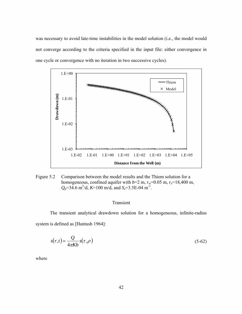
42
was necessary to avoid late-time instabilities in the model solution (i.e., the model would
not converge according to the criteria specified in the input file: either convergence in
one cycle or convergence with no iteration in two successive cycles).
Figure 5.2 Comparison between the model results and the Thiem solution for a homogeneous, confined aquifer with b=2 m, rw=0.05 m, re=18,400 m, Qp=34.6 m3/d, K=100 m/d, and Ss=3.5E-04 m-1.
Transient
The transient analytical drawdown solution for a homogeneous, infinite-radius
system is defined as [Hantush 1964]:
( ) ( )ρτπ
,4
, sKb
Qtrs = (5-62)
where
1.E-03
1.E-02
1.E-01
1.E+00
1.E-02 1.E-01 1.E+00 1.E+01 1.E+02 1.E+03 1.E+04 1.E+05
Dra
wdo
wn
(m)
Distance from the Well (m)
Thiem
Model
43
( ) ( )[ ] ( ) ( ) ( ) ( )[ ]( ) ( )[ ]∫
∞
+−−−
=0
21
21
20101
214, duuYuJu
uJuYuYuJuEXPs ρρτπ
ρτ (5-63)
and
wws rr
rSKt
== ρτ ;2 (5-64)
The Hantush solution (Eqns. 5-62 through 5-64) is based on the following assumptions
[Batu 1998]:
• The aquifer is homogeneous and isotropic;
• The aquifer is horizontal with a constant thickness (b);
• The aquifer is not leaky;
• The aquifer is infinite in horizontal extent;
• The well fully penetrates the aquifer; and
• The pumping rate of the well is constant.
The Hantush solution is applicable for all values of time and radial distances from the
well. A special case of the Hantush solution is defined for determining the drawdown at
the well-face (rw) [Lee 1998]:
( ) ( )( ) ( )( )∫
∞
+−−
=0
321
21
2
22
184
, dxxxrYxrJ
txEXPrKb
Qtrswww
wκ
ππ (5-65)
The Hantush equation may also be simplified provided that:
KSrt sw
230> (5-66)
44
to the Theis solution:
( ) ( )uWbK
Qtrsπ4
, = (5-67)
where W(u)=E1(u), the exponential integral, which is defined as:
( ) ( )∑∞
= ⋅−−−−=
1 !1ln5772.0
n
nn
nnuuuW (5-68)
The Theis solution has an additional assumption to those of the Hantush solution: the
diameter of the well is infinitesimally small compared to the horizontal extent; i.e.,
wellbore storage is negligible. Prior to the time defined by Eqn. 5-66, the Theis solution
is not applicable [Hantush 1964].
Comparison of the three analytical solutions (Eqns. 5-62, 5-65, and 5-67) for
drawdown at the well over time (Figure 5.3) show good agreement, especially as time
increases (for this comparison, the formulation specific to rw was employed). As
discussed, the Theis solution is not applicable at very small times. This is reflected in
comparing the drawdown at t=1.2E-08 days as determined using the Theis equation to the
Hantush results (RPD=23.1%) and numerical model results (RPD=22.9%). The average
RPD between the numerical model results and the Hantush results is 0.5%. At early time
(t=1.2E-06 d), the ME between the drawdown datasets is -8.7E-04 m, the MAE is 8.7E-
04 m, and the RMSE between the datasets 1.5E-03 m. These errors are small compared
to the actual drawdowns (from -0.88% to 1.5% at the well) indicating that errors in the
model are a small part of the overall model response. At late time (t=6.9 d), the ME
between the drawdown datasets is 1.1E-03 m, the MAE is 1.3E-03 m, and the RMSE
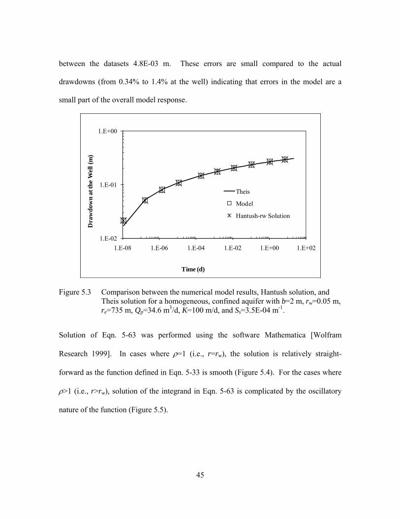
45
between the datasets 4.8E-03 m. These errors are small compared to the actual
drawdowns (from 0.34% to 1.4% at the well) indicating that errors in the model are a
small part of the overall model response.
Figure 5.3 Comparison between the numerical model results, Hantush solution, and Theis solution for a homogeneous, confined aquifer with b=2 m, rw=0.05 m, re=735 m, Qp=34.6 m3/d, K=100 m/d, and Ss=3.5E-04 m-1.
Solution of Eqn. 5-63 was performed using the software Mathematica [Wolfram
Research 1999]. In cases where ρ=1 (i.e., r=rw), the solution is relatively straight-
forward as the function defined in Eqn. 5-33 is smooth (Figure 5.4). For the cases where
ρ>1 (i.e., r>rw), solution of the integrand in Eqn. 5-63 is complicated by the oscillatory
nature of the function (Figure 5.5).
1.E-02
1.E-01
1.E+00
1.E-08 1.E-06 1.E-04 1.E-02 1.E+00 1.E+02
Dra
wdo
wn
at th
e W
ell (
m)
Time (d)
Theis
Model
Hantush-rw Solution

46
Figure 5.4 Function s(τ,ρ) where τ=1 and ρ=1.
Figure 5.5 Function s(τ,ρ) where τ=1 and ρ=2.
Comparison of the numerical model drawdown results across the aquifer for
selected times to the Hantush solution (general formulation) for those times as well as to
the Theis solution for the same times yields a similar pattern of agreement between the
different datasets (i.e., the datasets converge at later times and show small differences at
earlier times) (Figure 5.3). Despite the inability to accurately solve the general Hantush
500 1000 1500 2000 2500 3000u
0.00025
0.0005
0.00075
0.001
0.00125
0.0015
0.00175sHt ,rL
500 1000 1500 2000 2500 3000u
-1´ 10-6
1´ 10-6
2´ 10-6
sHt ,rL
s, r
s, r

47
formulation for all r>rw, it is clear from evaluating the numerical model results compared
to the Hantush results and the Theis results that the numerical model is behaving
consistently with these models (Figure 5.6).
Figure 5.6 Comparison between the numerical model results, Hantush solution, and Theis solution for a homogeneous, confined aquifer with b=2 m, rw=0.05 m, re=735 m, Qp=34.6 m3/d, K=100 m/d, and Ss=3.5E-04 m-1.
As was observed in the comparisons between the drawdown at the well solutions,
the deviation between the numerical model drawdown throughout the aquifer and the
analytical solutions is greatest at early times. It is important to note that while the values
of the numerical model drawdowns differ from the analytical solutions at these early
times, the shape of the drawdown curves for each solution series are consistent with one
another, further confirming that the model is behaving appropriately.
1.E-03
1.E-02
1.E-01
1.E+00
1.E-03 1.E-02 1.E-01 1.E+00 1.E+01 1.E+02 1.E+03
Dra
wdo
wn
(m)
Distance from Well (m)
Model
Theis
Hantusht = 1.02 st = 131 st = 9,400 st = 6.92 d
t = 0.015 s
t = 0.001 s

48
Hydraulic Diffusivity
As defined in Eqn. 5-4, hydraulic diffusivity (D) is a function of K and Ss. To
obtain the values of D for each layer, individual layer K-values were selected while the Ss
was generally determined as a function of K. In terms of real-world applications, it is
often unrealistic to assume that all aquifers and aquifer layers have the same Ss. Using
data compiled from readily available resources [Anderson and Woessner 1992; Maidment
1993], a relationship of Ss based on K was developed. This relationship was derived
based on visual inspection of the data set, which indicated that the data can be separated
into three K ranges. It is important to note this distinction as Ss is actually a function of
the matrix geometry and compressibility, not K. However, as both Ss and K are functions
of the matrix geometry, and geometry is related to compressibility, it is reasonable to
assume that the two parameters correlate. A simple regression was performed on the
three regions of the data to obtain an equation correlating Ss to K. This relationship
(Figure 5.7) is not intended to be definitive of all systems, but is used instead to give
approximate and reasonable estimates of Ss for the various scenarios modeled.
As stated in Chapter 2, in most applications, it is more important to accurately
identify high-K layers than low-K layers. For this reason, the scenarios in this study
focus primarily on K values of 1.0E-02 m/d and greater (sands and gravel). From Figure
5-7, this region is represented by a constant Ss relationship of 3.5E-04 1/m. As such, the
majority of scenarios considered herein employ Ss=3.5E-04 1/m, with modifications as
needed to illustrate certain behaviors later in this Chapter.

49
Figure 5.7 Correlation between K and Ss.
Numerical Definition of Quasi-Steady-State
For the purposes of this analysis, quasi-steady-state will be considered to have
been attained when the maximum relative percent difference between the gradients at the
well is approximately five percent (5%). This criterion was selected based on inspection
of several sets of preliminary results and an examination of the gradient behaviors over
time. The value of five percent was selected as the time when the gradients, when
plotted, ceased to change “appreciably”, with only small changes over large periods of
time observed (as discussed in Chapter 2). The maximum relative percent difference
(error) (RPD) is defined as:
Low K RangeSs=-145129K2+78.517K+0.0012R2=0.9985
Mid K RangeSs=3E-08K-1.6349R2 = 0.9698
1.E-05
1.E-04
1.E-03
1.E-02
1.E-01
1.E-08 1.E-06 1.E-04 1.E-02 1.E+00 1.E+02
S s(1
/m)
K (m/d)
High K RangeSs=3.53E-4
Gravel SandsSiltsClays

50
( ) 1002/
×+
−=
Gradient MaximumGradient MinimumGradient MaximumGradient MinimumRPD (5-21)
Summary of Scenarios
Throughout the course of the single-domain analyses, 96 different arrangements
of K and Ss were employed (Table 5.1). The remaining system variables are as described
in the text; each combination of K and Ss may be used with different system parameter
values as needed to illustrate different phenomena.

51
Tabl
e 5.
1 Su
mm
ary
of S
cena
rios.
Scen
ario
b (m
) a
K1
(m/d
) K
2 (m
/d)
K3
(m/d
) S s
1 (1
/m)
S s2
(1/m
) S s
3 (1
/m)
Qp
(L/m
in)
Δz
(m)
Q1
0.9
1 1
0.01
0.
2 3.
5E-0
4 3.
5E-0
4 3.
5E-0
4 0.
300
0.30
Q
2 0.
9 1
100
0.01
0.
2 3.
5E-0
4 3.
5E-0
4 3.
5E-0
4 0.
208
0.30
Q
3a
0.9
1 0.
01
0.00
01
0.00
2 3.
5E-0
4 3.
5E-0
4 3.
5E-0
4 0.
0030
0 0.
30
Q3b
1.
8 1
0.01
0.
0001
0.
002
3.5E
-04
3.5E
-04
3.5E
-04
0.00
600
0.30
Q
3c
3.6
1 0.
01
0.00
01
0.00
2 3.
5E-0
4 3.
5E-0
4 3.
5E-0
4 0.
0120
0 0.
30
Q3d
7.
2 1
0.01
0.
0001
0.
002
3.5E
-04
3.5E
-04
3.5E
-04
0.02
40
0.30
Q
3e
14.4
1
0.01
0.
0001
0.
002
3.5E
-04
3.5E
-04
3.5E
-04
0.04
80
0.60
Q
3f
28.8
1
0.01
0.
0001
0.
002
3.5E
-04
3.5E
-04
3.5E
-04
0.09
60
1.20
Q
4a
0.9
1 1
0.01
0.
2 3.
5E-0
4 3.
5E-0
4 3.
5E-0
4 0.
300
0.30
Q
4b
1.8
1 1
0.01
0.
2 3.
5E-0
4 3.
5E-0
4 3.
5E-0
4 0.
600
0.30
Q
4c
3.6
1 1
0.01
0.
2 3.
5E-0
4 3.
5E-0
4 3.
5E-0
4 1.
20
0.30
Q
4d
7.2
1 1
0.01
0.
2 3.
5E-0
4 3.
5E-0
4 3.
5E-0
4 2.
40
0.30
Q
4e
14.4
1
1 0.
01
0.2
3.5E
-04
3.5E
-04
3.5E
-04
4.80
0.
60
Q4f
28
.8
1 1
0.01
0.
2 3.
5E-0
4 3.
5E-0
4 3.
5E-0
4 9.
60
1.20
Q
5a
0.9
1 10
0 1
20
3.5E
-04
3.5E
-04
3.5E
-04
30.0
0.
30
Q5b
1.
8 1
100
1 20
3.
5E-0
4 3.
5E-0
4 3.
5E-0
4 60
.0
0.30
Q
5c
3.6
1 10
0 1
20
3.5E
-04
3.5E
-04
3.5E
-04
120
0.30
Q
5d
7.2
1 10
0 1
20
3.5E
-04
3.5E
-04
3.5E
-04
240
0.30
Q
5e
14.4
1
100
1 20
3.
5E-0
4 3.
5E-0
4 3.
5E-0
4 48
0 0.
60
Q5f
28
.8
1 10
0 1
20
3.5E
-04
3.5E
-04
3.5E
-04
960
1.20
Q
6a
0.9
1 10
,000
10
0 2,
000
3.5E
-04
3.5E
-04
3.5E
-04
2,99
9 0.
30
Q6b
1.
8 1
10,0
00
100
2,00
0 3.
5E-0
4 3.
5E-0
4 3.
5E-0
4 5,
999
0.30
Q
6c
3.6
1 10
,000
10
0 2,
000
3.5E
-04
3.5E
-04
3.5E
-04
11,9
97
0.30
Q
6d
7.2
1 10
,000
10
0 2,
000
3.5E
-04
3.5E
-04
3.5E
-04
23,9
94
0.30
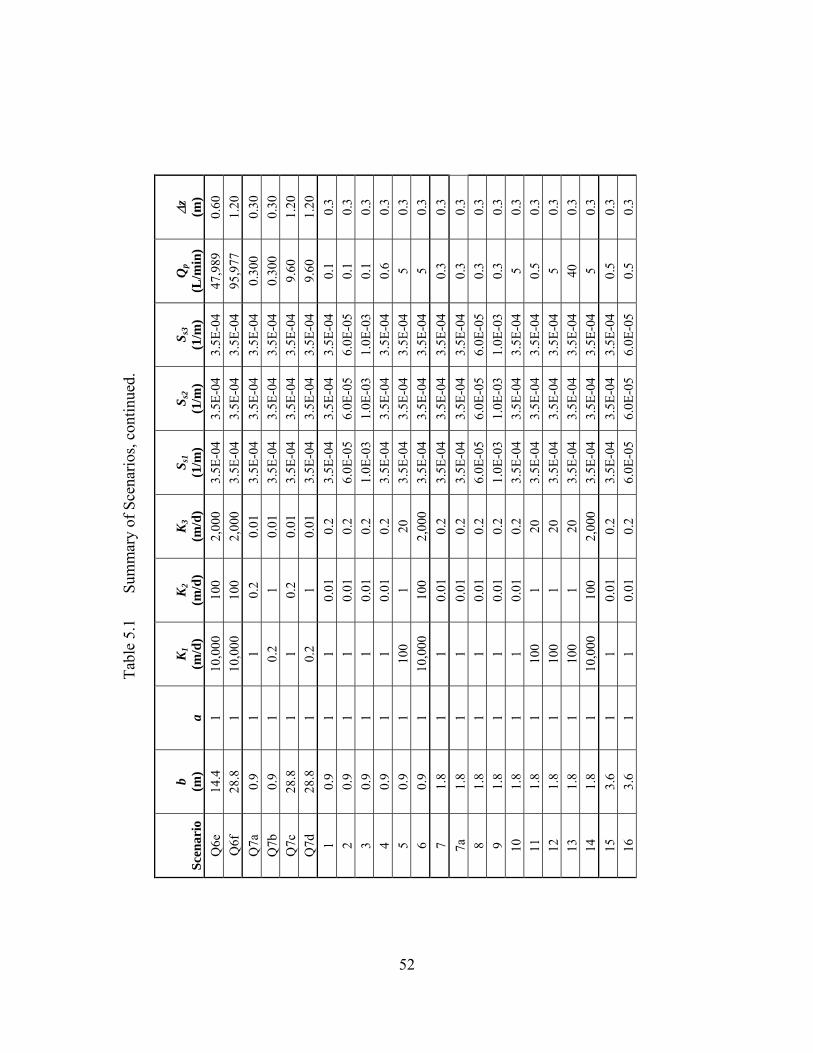
52
Tabl
e 5.
1 Su
mm
ary
of S
cena
rios,
cont
inue
d.
Scen
ario
b (m
) a
K1
(m/d
) K
2 (m
/d)
K3
(m/d
) S s
1 (1
/m)
S s2
(1/m
) S s
3 (1
/m)
Qp
(L/m
in)
Δz
(m)
Q6e
14
.4
1 10
,000
10
0 2,
000
3.5E
-04
3.5E
-04
3.5E
-04
47,9
89
0.60
Q
6f
28.8
1
10,0
00
100
2,00
0 3.
5E-0
4 3.
5E-0
4 3.
5E-0
4 95
,977
1.
20
Q7a
0.
9 1
1 0.
2 0.
01
3.5E
-04
3.5E
-04
3.5E
-04
0.30
0 0.
30
Q7b
0.
9 1
0.2
1 0.
01
3.5E
-04
3.5E
-04
3.5E
-04
0.30
0 0.
30
Q7c
28
.8
1 1
0.2
0.01
3.
5E-0
4 3.
5E-0
4 3.
5E-0
4 9.
60
1.20
Q
7d
28.8
1
0.2
1 0.
01
3.5E
-04
3.5E
-04
3.5E
-04
9.60
1.
20
1 0.
9 1
1 0.
01
0.2
3.5E
-04
3.5E
-04
3.5E
-04
0.1
0.3
2 0.
9 1
1 0.
01
0.2
6.0E
-05
6.0E
-05
6.0E
-05
0.1
0.3
3 0.
9 1
1 0.
01
0.2
1.0E
-03
1.0E
-03
1.0E
-03
0.1
0.3
4 0.
9 1
1 0.
01
0.2
3.5E
-04
3.5E
-04
3.5E
-04
0.6
0.3
5 0.
9 1
100
1 20
3.
5E-0
4 3.
5E-0
4 3.
5E-0
4 5
0.3
6 0.
9 1
10,0
00
100
2,00
0 3.
5E-0
4 3.
5E-0
4 3.
5E-0
4 5
0.3
7 1.
8 1
1 0.
01
0.2
3.5E
-04
3.5E
-04
3.5E
-04
0.3
0.3
7a
1.8
1 1
0.01
0.
2 3.
5E-0
4 3.
5E-0
4 3.
5E-0
4 0.
3 0.
3 8
1.8
1 1
0.01
0.
2 6.
0E-0
5 6.
0E-0
5 6.
0E-0
5 0.
3 0.
3 9
1.8
1 1
0.01
0.
2 1.
0E-0
3 1.
0E-0
3 1.
0E-0
3 0.
3 0.
3 10
1.
8 1
1 0.
01
0.2
3.5E
-04
3.5E
-04
3.5E
-04
5 0.
3 11
1.
8 1
100
1 20
3.
5E-0
4 3.
5E-0
4 3.
5E-0
4 0.
5 0.
3 12
1.
8 1
100
1 20
3.
5E-0
4 3.
5E-0
4 3.
5E-0
4 5
0.3
13
1.8
1 10
0 1
20
3.5E
-04
3.5E
-04
3.5E
-04
40
0.3
14
1.8
1 10
,000
10
0 2,
000
3.5E
-04
3.5E
-04
3.5E
-04
5 0.
3 15
3.
6 1
1 0.
01
0.2
3.5E
-04
3.5E
-04
3.5E
-04
0.5
0.3
16
3.6
1 1
0.01
0.
2 6.
0E-0
5 6.
0E-0
5 6.
0E-0
5 0.
5 0.
3

53
Tabl
e 5.
1 Su
mm
ary
of S
cena
rios,
cont
inue
d.
Scen
ario
b (m
) a
K1
(m/d
) K
2 (m
/d)
K3
(m/d
) S s
1 (1
/m)
S s2
(1/m
) S s
3 (1
/m)
Qp
(L/m
in)
Δz
(m)
17
3.6
1 1
0.01
0.
2 1.
0E-0
3 1.
0E-0
3 1.
0E-0
3 0.
5 0.
3 18
3.
6 1
1 0.
01
0.2
3.5E
-04
3.5E
-04
3.5E
-04
5 0.
3 18
a 3.
6 1
1 0.
01
0.2
3.5E
-04
3.5E
-04
3.5E
-04
5 0.
3 19
3.
6 1
1 0.
01
0.2
3.5E
-04
3.5E
-04
3.5E
-04
10
0.3
20
3.6
1 10
0 1
20
3.5E
-04
3.5E
-04
3.5E
-04
5 0.
3 21
3.
6 1
10,0
00
100
2,00
0 3.
5E-0
4 3.
5E-0
4 3.
5E-0
4 5
0.3
22a
7.2
1 1
0.01
0.
2 3.
5E-0
4 3.
5E-0
4 3.
5E-0
4 1
0.3
23a
7.2
1 1
0.01
0.
2 6.
0E-0
5 6.
0E-0
5 6.
0E-0
5 1
0.3
24a
7.2
1 1
0.01
0.
2 1.
0E-0
3 1.
0E-0
3 1.
0E-0
3 1
0.3
22b
7.2
1 10
0.
1 2
3.3E
-03
3.3E
-03
3.3E
-03
1 0.
3 23
b 7.
2 1
10
0.1
2 6.
0E-0
4 6.
0E-0
4 6.
0E-0
4 1
0.3
24b
7.2
1 10
0.
1 2
1.0E
-02
1.0E
-02
1.0E
-02
1 0.
3 25
7.
2 1
1 0.
01
0.2
3.5E
-04
3.5E
-04
3.5E
-04
5 0.
3 25
a 7.
2 1
1 0.
01
0.2
3.5E
-04
3.5E
-04
3.5E
-04
5 0.
3 25
b 7.
2 1
1 0.
01
0.2
3.5E
-04
3.5E
-04
3.5E
-04
5 0.
3 25
c 7.
2 1
1 0.
01
0.2
3.5E
-04
3.5E
-04
3.5E
-04
5 0.
3 26
7.
2 1
1 0.
01
0.2
3.5E
-04
3.5E
-04
3.5E
-04
10
0.3
27
7.2
1 10
0 1
20
3.5E
-04
3.5E
-04
3.5E
-04
5 0.
3 28
7.
2 1
10,0
00
100
2,00
0 3.
5E-0
4 3.
5E-0
4 3.
5E-0
4 5
0.3
29
14.4
1
1 0.
01
0.2
3.5E
-04
3.5E
-04
3.5E
-04
5 0.
6 30
14
.4
1 1
0.01
0.
2 6.
0E-0
5 6.
0E-0
5 6.
0E-0
5 5
0.6
31
14.4
1
1 0.
01
0.2
1.0E
-03
1.0E
-03
1.0E
-03
5 0.
6 32
14
.4
1 10
0 1
20
3.5E
-04
3.5E
-04
3.5E
-04
5 0.
6 33
14
.4
1 10
,000
10
0 2,
000
3.5E
-04
3.5E
-04
3.5E
-04
5 0.
6
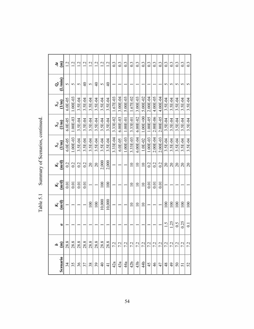
54
Tabl
e 5.
1 Su
mm
ary
of S
cena
rios,
cont
inue
d.
Scen
ario
b (m
) a
K1
(m/d
) K
2 (m
/d)
K3
(m/d
) S s
1 (1
/m)
S s2
(1/m
) S s
3 (1
/m)
Qp
(L/m
in)
Δz
(m)
34
28.8
1
1 0.
01
0.2
6.0E
-05
6.0E
-05
6.0E
-05
5 1.
2 35
28
.8
1 1
0.01
0.
2 1.
00E-
03
1.00
E-03
1.
00E-
03
5 1.
2 36
28
.8
1 1
0.01
0.
2 3.
5E-0
4 3.
5E-0
4 3.
5E-0
4 5
1.2
37
28.8
1
1 0.
01
0.2
3.5E
-04
3.5E
-04
3.5E
-04
40
1.2
38
28.8
1
100
1 20
3.
5E-0
4 3.
5E-0
4 3.
5E-0
4 5
1.2
39
28.8
1
100
1 20
3.
5E-0
4 3.
5E-0
4 3.
5E-0
4 40
1.
2 40
28
.8
1 10
,000
10
0 2,
000
3.5E
-04
3.5E
-04
3.5E
-04
5 1.
2 41
28
.8
1 10
,000
10
0 2,
000
3.5E
-04
3.5E
-04
3.5E
-04
40
1.2
42a
7.2
1 1
1 1
3.33
E-04
3.
33E-
02
1.67
E-03
1
0.3
43a
7.2
1 1
1 1
6.0E
-05
6.00
E-03
3.
00E-
04
1 0.
3 44
a 7.
2 1
1 1
1 1.
00E-
03
1.00
E-01
5.
00E-
03
1 0.
3 42
b 7.
2 1
10
10
10
3.33
E-03
3.
33E-
01
1.67
E-02
1
0.3
43b
7.2
1 10
10
10
6.
00E-
04
6.00
E-02
3.
00E-
03
1 0.
3 44
b 7.
2 1
10
10
10
1.0E
-02
1.00
E+00
5.
00E-
02
1 0.
3 45
7.
2 1
1 0.
01
0.2
1.00
E-03
1.
00E-
05
2.00
E-04
1
0.3
46
7.2
1 1
0.01
0.
2 2.
00E-
04
2.00
E-06
4.
00E-
05
1 0.
3 47
7.
2 1
1 0.
01
0.2
2.00
E-03
2.
00E-
05
4.00
E-04
1
0.3
48
7.2
1.5
100
1 20
3.
5E-0
4 3.
5E-0
4 3.
5E-0
4 5
0.3
49
7.2
1.25
10
0 1
20
3.5E
-04
3.5E
-04
3.5E
-04
5 0.
3 50
7.
2 0.
5 10
0 1
20
3.5E
-04
3.5E
-04
3.5E
-04
5 0.
3 51
7.
2 0.
25
100
1 20
3.
5E-0
4 3.
5E-0
4 3.
5E-0
4 5
0.3
52
7.2
0.1
100
1 20
3.
5E-0
4 3.
5E-0
4 3.
5E-0
4 5
0.3
55
As can be seen in Table 5.1, the simulations employed in this study are focused
on the higher-K regions of the correlation relationship. This is appropriate as the
flowmeter is typically used to determine the dominant regions of flow within an aquifer;
layers with K less than 1.0E-04 m/d would be considered to be no-flow layers in a
practical sense (i.e., clays or consolidated materials), thereby creating multi-aquifer
systems rather than multi-layer systems. A robust body of research exists to describe
multi-aquifer systems and therefore they are not dealt with in this study. Additionally,
with the exception of boundary effects, flow in multi-layer aquifers is generally assumed
to be horizontal with no crossflow occurring between the layers.
Results and Discussion
Once pumping commences and water is removed from the higher-K layer(s),
water begins to be released from storage in the lower-K layer(s) into the higher-K
layer(s). Eventually, the hydraulic gradients near the well in each layer become equal
and constant, indicating that the system has attained quasi-steady-state (Scenario Q1;
Figure 5.8). In Figure 5.8, crossflow is indicated by the changing hydraulic head
gradients for each layer at early times. Numerically, hydraulic head gradients at the well
will be considered to have attained quasi-steady-state when the maximum RPD between
any two grid-layer’s hydraulic gradients at the well is less than 5%. The hydraulic
gradients at the well for the system shown in Figure 5.8 attained quasi-steady-state at
9.3E+02 seconds (1.6E+01 minutes).

56
Figure 5.8 Gradients at the well for selected grid-layers as a function of time for Scenario Q1.
Having reached quasi-steady-state does not imply that the entire system has
reached steady-state. For the system depicted in Figure 5.8, quasi-steady-state of the
gradients at the well was attained at t=9.3E+02 seconds (1.6E+01 minutes), while steady-
state drawdown at the well was attained after t=8.6E+02 days (obtained from the model
output; the model terminates at the system steady-state). This difference between the
time to reach quasi-steady-state and steady-state implies that crossflow is an early-time
phenomenon that occurs close to the well.
As can be seen from results presented in Figure 5.9, the use of an arithmetic
average K (used in the analytical model) to describe the overall system behavior is valid
during the early time of this study (i.e., the analytical model and the numerical model
results are approximate to each other).
-4.0
-3.5
-3.0
-2.5
-2.0
0.E+00 2.E+02 4.E+02 6.E+02 8.E+02 1.E+03
Hyd
raul
ic G
radi
ent a
t the
Wel
l
Time (s)
Layer 1 (K=1 m/d)
Layer 2 (K=0.01 m/d)
Layer 3 (K=0.2 m/d)
tQSS = 933 s

57
Figure 5.9 Drawdown at the well as a function of time for Scenario Q1. Analytical solution – solid squares; model solution: solid line.
These results also confirm the results published by Katz and Tek [1962], who
found that the arithmetic average of the layer K values may be used to accurately predict
multi-layer system behaviors at early times.
To evaluate the dominance of the horizontal flow from higher-K (higher-D) layers
compared to the influence of crossflow, the high-K layer from Scenario Q1 was further
increased by a factor of 100 (Scenario 2Q), with all other parameters maintained the same
as in Scenario Q1. By examining the early-time hydraulic gradients for Scenario Q2
(Figure 5.10), it can be seen that the hydraulic gradients at the well in the higher-K layer
remain essentially constant, implying that crossflow into this layer is negligible compared
to the horizontal flow from this layer. In contrast, the hydraulic gradients in the lower-K
1.E-01
1.E+00
1.E+01
1.E-05 1.E-04 1.E-03 1.E-02 1.E-01 1.E+00 1.E+01 1.E+02
Dra
wdo
wn
at th
e W
ell (
m)
Time (d)
Theis
Model
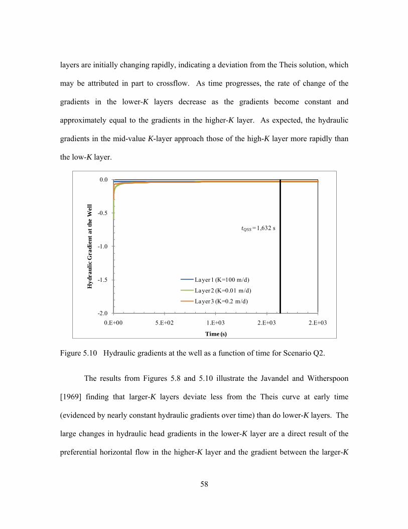
58
layers are initially changing rapidly, indicating a deviation from the Theis solution, which
may be attributed in part to crossflow. As time progresses, the rate of change of the
gradients in the lower-K layers decrease as the gradients become constant and
approximately equal to the gradients in the higher-K layer. As expected, the hydraulic
gradients in the mid-value K-layer approach those of the high-K layer more rapidly than
the low-K layer.
Figure 5.10 Hydraulic gradients at the well as a function of time for Scenario Q2.
The results from Figures 5.8 and 5.10 illustrate the Javandel and Witherspoon
[1969] finding that larger-K layers deviate less from the Theis curve at early time
(evidenced by nearly constant hydraulic gradients over time) than do lower-K layers. The
large changes in hydraulic head gradients in the lower-K layer are a direct result of the
preferential horizontal flow in the higher-K layer and the gradient between the larger-K
-2.0
-1.5
-1.0
-0.5
0.0
0.E+00 5.E+02 1.E+03 2.E+03 2.E+03
Hyd
raul
ic G
radi
ent a
t the
Wel
l
Time (s)
Layer 1 (K=100 m/d)
Layer 2 (K=0.01 m/d)
Layer 3 (K=0.2 m/d)
tQSS = 1,632 s
59
and lower-K layers generating a vertical flow component. The magnitude of the
crossflow out of the lower-K layer and into the higher-K layer is much less than the
magnitude of the horizontal flow from the larger-K layer, resulting in hydraulic gradients
in the larger-K layer that remain essentially constant. In contrast, the amount of water
leaving the lower-K layer due to cross-flow is proportionally a much larger component of
the overall behavior of the lower-K layer, resulting in hydraulic gradients that change
appreciably initially.
In comparing the behaviors of Scenario Q1 (Figure 5.8) and Scenario Q2 (Figure
5.10), the lower-K layer in Scenario Q2 has a larger overall influence on the time
required for the system to attain quasi-steady-state (2.7E+01 minutes for Scenario Q2 and
1.5E+01 minutes for Scenario Q1) due to the larger influence of crossflow in the lower-K
layers in Scenario Q2 than is observed from the lower-K layer in Scenario Q1. This
phenomenon is most clearly illustrated by observing the flows out of each layer (Figures
5.11 and 5.12 for Scenario Q1 and Scenario Q2, respectively). In these figures, the flow
out of the high-K layer is essentially constant for both scenarios. However, the flows out
of the lower-K layers are characterized by a period of fluctuation followed by steady
flow. The fluctuation is the result of vertical crossflow. This period of fluctuation is
longer and with larger fluctuations for Scenario Q2, due to the crossflow being
proportionally larger in these layers.
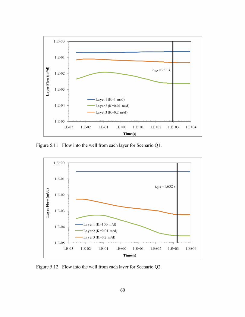
60
Figure 5.11 Flow into the well from each layer for Scenario Q1.
Figure 5.12 Flow into the well from each layer for Scenario Q2.
1.E-05
1.E-04
1.E-03
1.E-02
1.E-01
1.E+00
1.E-03 1.E-02 1.E-01 1.E+00 1.E+01 1.E+02 1.E+03 1.E+04
Lay
er F
low
(m3 /
d)
Time (s)
Layer 1 (K=1 m/d)
Layer 2 (K=0.01 m/d)
Layer 3 (K=0.2 m/d)
tQSS = 933 s
1.E-05
1.E-04
1.E-03
1.E-02
1.E-01
1.E+00
1.E-03 1.E-02 1.E-01 1.E+00 1.E+01 1.E+02 1.E+03 1.E+04
Lay
er F
low
(m3 /
d)
Time (s)
Layer 1 (K=100 m/d)
Layer 2 (K=0.01 m/d)
Layer 3 (K=0.2 m/d)
tQSS = 1,632 s

61
This early transient behavior of the hydraulic gradients (influenced by crossflow)
is the cause of the system’s drawdown deviating from the Theis solution. The Theis
solution becomes approximate once the system attains quasi-steady-state and all flow is
horizontal and proportional to the layer transmissivity. This is again consistent with the
results found by Javandel and Witherspoon [1969]. Examination of Figures 5.8 and 5.10
illustrates the non-uniform behavior of the hydraulic gradients at early times. This
behavior becomes more prominent in lower-K layers as the hydraulic diffusivity between
the layers increases, for the reasons described above. The initially larger gradients in the
lower-K layers also explain why the flows from the lower-K layers are initially higher
than their steady-state values.
In determining the transient response behavior of the entire aquifer, it is useful to
examine the maximum RPD between the layer hydraulic gradients as a function of time
(Figure 5.13). By examining this relationship, it is apparent that the rate of change in the
difference between gradients decreases with time. This type of relationship holds true for
each of the systems examined during this study.

62
Figure 5.13 Maximum RPD in layer hydraulic gradients at the well as a function of time for Scenario Q1 and Scenario Q2.
Yet another way to look at the transient effects of pumping on an aquifer is to
compare the calculated K for each layer compared to the input layer K’s. This is
accomplished using Eqn. 2-3, modified such that the ambient flow is removed from the
equation, since no ambient flow occurs in this study:
bQzQKK
P
iii /
/ ΔΔ>=< (5-69)
Using equation 5.69, the individual layer K values were calculated using the
model output, flow from each layer at the well face. These calculated layer K values
were then normalized by the input layer K values to assess the relative effect of taking
flowmeter measurements before quasi-steady-state (Figure 5.14).
0%
20%
40%
60%
80%
100%
120%
140%
160%
180%
200%
1.E+00 1.E+01 1.E+02 1.E+03 1.E+04
Rel
ativ
e Per
cent
Dif
fere
nce
Bet
wee
n L
ayer
H
ydra
ulic
Gra
dien
ts
Time (s)
Scenario Q1
Scenario Q2 tQSS = 933 s
tQSS = 1,632 s

63
Figure 5.14 Ratio between calculated and model input layer K values for Scenario Q1.
As can be seen in Figure 5.14, the calculated layer K values initially differ from
the input layer K values, but rapidly approach the input values as shown by the values
approaching 1. The early differences are largest in the lowest-K layer (Layer 2). The
ratios also show that the lower-K layers initially yield inflated calculated K’s (i.e., K-
values larger than the model input values), while the high-K layer is underestimated.
This finding is again tied to the crossflow phenomenon. The importance of the
differences between the calculated and model input layer-K values will be examined in
greater detail in later in this chapter.
Aquifer Thickness Effects
A series of aquifer systems were modeled to determine the effect of overall
aquifer thickness (b) on the time required for the hydraulic gradients to attain quasi-
0.0
1.0
2.0
3.0
4.0
5.0
0.E+00 2.E+02 4.E+02 6.E+02 8.E+02 1.E+03
Rat
io o
f Cal
cula
ted
Lay
er K
to I
nput
K
Time (s)
Layer 1 (K=1 m/d)
Layer 2 (K=0.01 m/d)
Layer 3 (K=0.2 m/d)
tQSS = 933 s
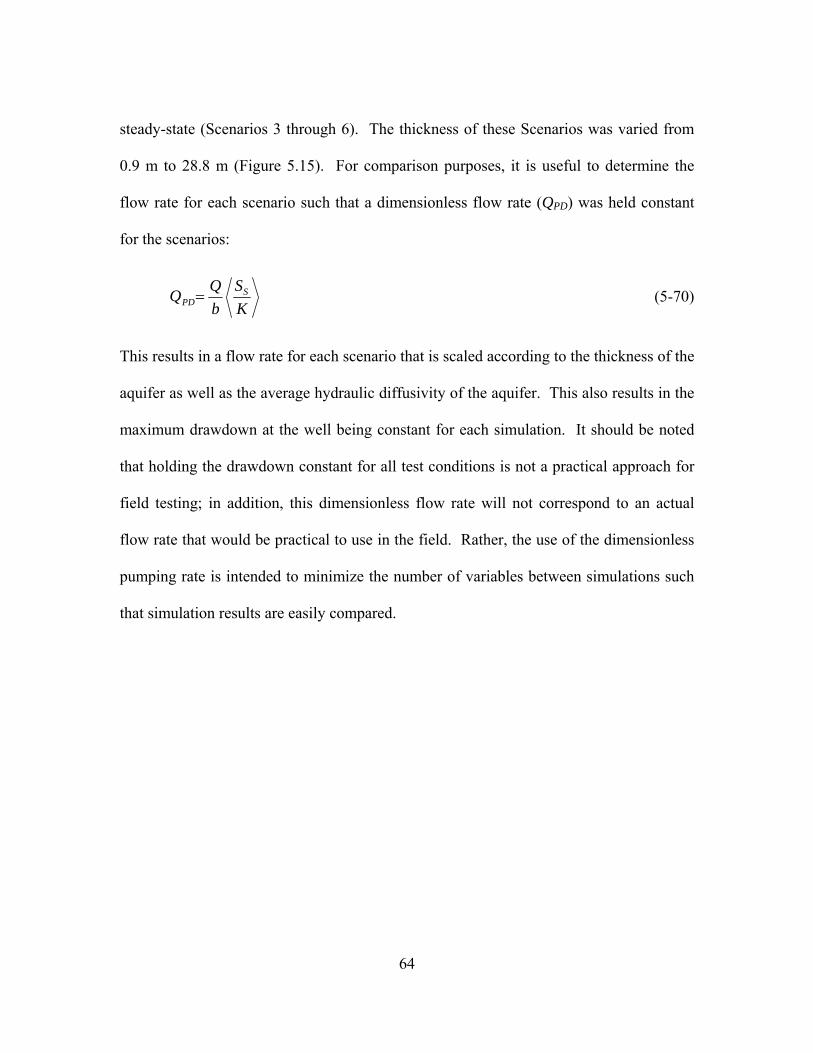
64
steady-state (Scenarios 3 through 6). The thickness of these Scenarios was varied from
0.9 m to 28.8 m (Figure 5.15). For comparison purposes, it is useful to determine the
flow rate for each scenario such that a dimensionless flow rate (QPD) was held constant
for the scenarios:
KS
bQQ S
PD= (5-70)
This results in a flow rate for each scenario that is scaled according to the thickness of the
aquifer as well as the average hydraulic diffusivity of the aquifer. This also results in the
maximum drawdown at the well being constant for each simulation. It should be noted
that holding the drawdown constant for all test conditions is not a practical approach for
field testing; in addition, this dimensionless flow rate will not correspond to an actual
flow rate that would be practical to use in the field. Rather, the use of the dimensionless
pumping rate is intended to minimize the number of variables between simulations such
that simulation results are easily compared.

65
Figure 5.15 Time to quasi-steady-state for Scenarios Q3-Q6 (with varying aquifer thicknesses, b).
The times to quasi-steady-state for each of the four scenarios results shown in
Figure 5.15 indicate that the time to attain quasi-steady-state is a function of the ratio of
the hydraulic diffusivities (D) between the layers as well as the overall aquifer thickness
(b). For each of the four scenarios, as b is increased, the time to quasi-steady-state
increases according to a power relationship.
The average power of the four relationships is 1.72, indicating that the increase in
the time required to attain quasi-steady-state is small at smaller thicknesses and becomes
larger between successive increases in aquifer thickness. Having a power relationship
implies that there is no theoretical bound on the time required to attain quasi-steady-state
as the aquifer thickness approaches infinity. In reality, however, there may be many
mechanisms that will influence the time to quasi-steady-state.
t = 111,274b1.73
R² = 1.00
t = 1,029b1.76
R² = 1.00
t = 11.0b1.73
R² = 1.00
t = 0.137b1.65
R² = 1.00
1.E-01
1.E+00
1.E+01
1.E+02
1.E+03
1.E+04
1.E+05
1.E+06
1.E+07
1.E+08
0 10 20 30 40 50
Tim
e to
Qua
si-S
tead
y-St
ate
(s)
Aquifer Thickness, b (m)
Scenario Q3 Scenario Q4Scenario Q5 Scenario Q6

66
This same exercise was performed using the same scenario parameters but with
flow rates typical of EBF testing (0.1 to 5 L/min, see Table 5.1). These simulations
(Figure 5.16) yield similar results and consistent conclusions to those observed in Figure
5.15. The Scenario Series are defined as:
Scenario Series Scenarios A 1, 7, 15, 22a, 29, 38
B 5, 11, 20, 27, 32, 40
C 6, 14, 21, 28, 33, 42
Figure 5.16 Time to quasi-steady-state for Scenario Series A, B, and C (with varying aquifer thicknesses, b).
t = 1,047b1.76
R² 1.00
t = 10.7b1.82
R² = 1.00
t = 0.123b1.98
R² = 1.00
1.E-01
1.E+00
1.E+01
1.E+02
1.E+03
1.E+04
1.E+05
1.E+06
1.E+07
1.E+08
0 10 20 30 40 50
Tim
e to
Qua
si-S
tead
y-St
ate
(s)
Aquifer Thickness (m)
Scenario Series AScenario Series BScenario Series C
67
Layer Thickness Effects
Having examined the effect of aquifer thickness on the time required to attain
quasi-steady-state, understanding how layer thickness affects the time to quasi-steady-
state is the next natural step. To assess the effect of layer thickness, the layers in
Scenario 25 were made successively thinner, with keeping the same K-value distribution
(Table 5.2). The times to quasi-steady-state for Scenarios 25 are also presented in Figure
5.17. These results show that as the layer thickness is decreased, the time to quasi-
steady-state decreases in a linear fashion.

68
Table 5.2 Summary of Layer Thickness Scenarios and Times to Quasi-Steady-State.
Scenario Layer-K Values Depth
(m) 25 25a 25b 25c 7.05 1 1 1 1 6.75 1 1 1 0.01 6.45 1 1 0.01 0.2 6.15 1 1 0.01 1 5.85 1 0.01 0.2 0.01 5.55 1 0.01 0.2 0.2 5.25 1 0.01 1 1 4.95 1 0.01 1 0.01 4.65 0.01 0.2 0.01 0.2 4.35 0.01 0.2 0.01 1 4.05 0.01 0.2 0.2 0.01 3.75 0.01 0.2 0.2 0.2 3.45 0.01 1 1 1 3.15 0.01 1 1 0.01 2.85 0.01 1 0.01 0.2 2.55 0.01 1 0.01 1 2.25 0.2 0.01 0.2 0.01 1.95 0.2 0.01 0.2 0.2 1.65 0.2 0.01 1 1 1.35 0.2 0.01 1 0.01 1.05 0.2 0.2 0.01 0.2 0.75 0.2 0.2 0.01 1 0.45 0.2 0.2 0.2 0.01 0.15 0.2 0.2 0.2 0.2
tQSS (s) 32,365 16,478 7,827 3,161

69
Figure 5.17 Time to quasi-steady-state for Scenario 25 (with varying layer thicknesses).
It is important to note that while the time to quasi-steady-state decreases with
decreasing layer thickness, it does not decrease to the same time to quasi-steady-state as
systems with similar layer thicknesses, but with only one set of layers (Table 5.3). In
Table 5.3, layer-K values for selected scenarios are rearranged to yield the same thickness
and pattern as Scenario Q1 (a 90 m scenario). The times to quasi-steady-state for the
scenarios in Table 5.3 are presented in Figure 5.18. Again, as the layer thickness is
decreased, the time to quasi-steady-state decreases; however the times remain greater
than that for the minimum scenario (Scenario Q1). This reinforces the conclusions from
the aquifer thickness analysis that as the overall aquifer thickness is increased, the time to
quasi-steady-state increases.
t = 13,830b - 601R² = 0.999
1.E+02
1.E+03
1.E+04
1.E+05
1.E-01 1.E+00 1.E+01
Tim
e to
Qua
si-S
tead
y-St
ate
(s)
Layer Thickness, b (m)
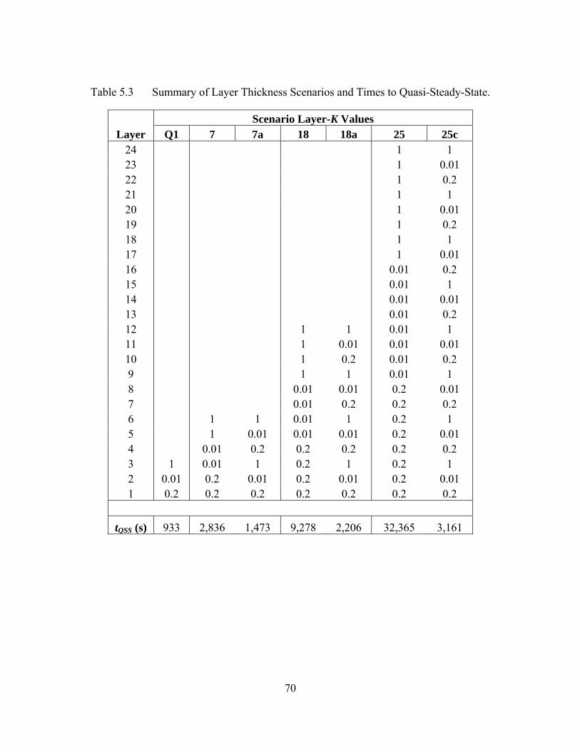
70
Table 5.3 Summary of Layer Thickness Scenarios and Times to Quasi-Steady-State.
Scenario Layer-K Values Layer Q1 7 7a 18 18a 25 25c
24 1 1 23 1 0.01 22 1 0.2 21 1 1 20 1 0.01 19 1 0.2 18 1 1 17 1 0.01 16 0.01 0.2 15 0.01 1 14 0.01 0.01 13 0.01 0.2 12 1 1 0.01 1 11 1 0.01 0.01 0.01 10 1 0.2 0.01 0.2 9 1 1 0.01 1 8 0.01 0.01 0.2 0.01 7 0.01 0.2 0.2 0.2 6 1 1 0.01 1 0.2 1 5 1 0.01 0.01 0.01 0.2 0.01 4 0.01 0.2 0.2 0.2 0.2 0.2 3 1 0.01 1 0.2 1 0.2 1 2 0.01 0.2 0.01 0.2 0.01 0.2 0.01 1 0.2 0.2 0.2 0.2 0.2 0.2 0.2
tQSS (s) 933 2,836 1,473 9,278 2,206 32,365 3,161

71
Figure 5.18 Time to quasi-steady-state for Table 5.3 scenarios.
Pumping Rate Effects
To assess the effect of pumping rate, QP, on the time required for a system to
attain quasi-steady-state, the QP in several scenarios was systematically increased (Table
5.4; see Table 5.1 for other parameter definitions). It should be noted that several of the
pumping rates employed for the model scenarios are unrealistically high and were
evaluated for mathematical purposes only (e.g., Scenarios Q5 and Q6).
In general, increasing the QP resulted in small differences in the time required to
attain quasi-steady-state. These differences, with the exception of the thickest systems
with the smallest layer-K values (Scenarios Q4f, 36, and 37) with the smallest pumping
rates, are not significant with respect to real-world application.
t = 1,078b1.71
R² = 0.999
t = 1,017b0.59
R² = 0.997
1.E+02
1.E+03
1.E+04
1.E+05
1.E-01 1.E+00 1.E+01
Tim
e to
Qua
si-S
tead
y-St
ate
(s)
Aquifer Thickness, b (m)
Scenarios Q1, 7, 18, 25
Scenarios Q1, 7a, 18a, and 25a

72
Table 5.4 Summary of Layer Arrangement Scenario Times to Quasi-Steady-State.
Scenario b
(m) K1
(m/d) K2
(m/d) K3
(m/d) Qp
(L/min)
5% RPD tQSS (s)
1 0.9 1 0.01 0.2 0.1 916 Q4a 0.9 1 0.01 0.2 0.3 933
4 0.9 1 0.01 0.2 0.6 916 5 0.9 100 1 20 5 9.09
Q5a 0.9 100 1 20 30 10.0 6 0.9 10,000 100 2,000 5 0.127
Q6a 0.9 10,000 100 2,000 2,999 0.127 7 1.8 1 0.01 0.2 0.3 2,836
Q4b 1.8 1 0.01 0.2 0.6 2,886 10 1.8 1 0.01 0.2 5 2,853 11 1.8 100 1 20 0.5 36.4 12 1.8 100 1 20 5 33.9 13 1.8 100 1 20 40 36.4
Q5b 1.8 100 1 20 60 29.0 14 1.8 10,000 100 2,000 5 0.35
Q6b 1.8 10,000 100 2,000 5,999 0.38 15 3.6 1 0.01 0.2 0.5 9,733
Q4c 3.6 1 0.01 0.2 1 9,716 18 3.6 1 0.01 0.2 5 9,278 19 3.6 1 0.01 0.2 10 9,300 20 3.6 100 1 20 5 98.3
Q5c 3.6 100 1 20 120 98.3 21 3.6 10,000 100 2,000 5 1.31
Q6c 3.6 10,000 100 2,000 11,997 0.96 22a 7.2 1 0.01 0.2 1 32,365 Q4d 7.2 1 0.01 0.2 2 32,219 25 7.2 1 0.01 0.2 5 32,106 26 7.2 1 0.01 0.2 10 32,468 27 7.2 100 1 20 5 334
Q5d 7.2 100 1 20 240 322 28 7.2 10,000 100 2,000 5 5.38
Q6d 7.2 10,000 100 2,000 23,994 3.22 32 14.4 100 1 20 5 1,306
Q5e 14.4 100 1 20 480 1,115 33 14.4 10,000 100 2,000 5 24.3
Q6e 14.4 10,000 100 2,000 47,989 11.4

73
Table 5.4 Summary of Layer Arrangement Scenario Times to Quasi-Steady-State, continued.
Scenario b
(m) K1
(m/d) K2
(m/d) K3
(m/d) Qp
(L/min)
5% RPD tQSS (s)
Q4f 28.8 1 0.01 0.2 0.1 522,280 Q4f 28.8 1 0.01 0.2 0.5 435,074 Q4f 28.8 1 0.01 0.2 0.5 416,736 36 28.8 1 0.01 0.2 5 398,507
Q4f 28.8 1 0.01 0.2 10 398,857 37 28.8 1 0.01 0.2 40 397,241 38 28.8 100 1 20 5 5,803 39 28.8 100 1 20 40 4,419
Q5f 28.8 100 1 20 960 3,990 40 28.8 10,000 100 2,000 5 111 41 28.8 10,000 100 2,000 40 88.1
Q6f 28.8 10,000 100 2,000 95,977 39.9
Based on these findings, pumping rate is not considered to be a significant factor
in the time needed to attain quasi-steady-state, and therefore, the pumping rate should be
selected based on the study limitations (i.e., time, purge water disposal costs/options,
etc.).
Layer Arrangement Effects
As discussed previously, the contrast in D between layers is an important factor in
the time required for a multi-layer aquifer to attain quasi-steady-state under pumping
conditions. Now, the impact that layer placement has on the time required for a system to
attain quasi-steady-state will be addressed. The systems used in this analysis are
Scenarios Q4a, Q7a, Q7b, and Q4f, Q7c, and Q7d. In each of the three scenarios, the

74
layers are of equal thickness. Two overall aquifer thicknesses were evaluated for the
scenarios: (a) b=0.9 m and (b) b=28.8 m.
As with previous simulations, a QPD=4.2E-04 was employed. The layer
arrangement is a factor in the time required for systems to attain quasi-steady-state. The
times to quasi-steady-state (tQSS) for each of the scenarios are provided in Table 5.5; the
RPD between the scenario with the minimum time to quasi-steady-state and the other two
scenarios for the two thicknesses is also provided. The differences in the times for the
thin aquifer (Scenarios Q4a, Q7a, and Q7b), although having RPDs of 6.2% and 3.3% are
not significant in terms of real-world application as they differ from the scenario with the
shortest time to quasi-steady-state by less than 2 minutes. In thicker systems (Scenarios
Q4f, Q7c, and Q7d), similar RPDs were observed (8.4% and 8.5%), but with the time
required to reach quasi-steady-state being much larger (by approximately three orders of
magnitude) than the thin systems. Unlike with the thin systems, the differences between
the three thicker systems is significant in real-world application as there is approximately
10 hours difference between the time to quasi-steady-state required for Scenario Q4f and
the other two scenarios.
Table 5.5 Summary of Layer Arrangements and Times to Quasi-Steady-State.
Scenario b (m) tQSS (s) Q4a 0.9 9.3E+02 Q7a 0.9 9.9E+02 Q7b 0.9 9.0E+02
Q4f 28.8 4.0E+05 Q7c 28.8 4.3E+05 Q7d 28.8 4.3E+05

75
The scenarios with largest times to quasi-steady-state are those where the lower-K
layers are adjacent to one another with the lowest-K layer located adjacent to a boundary
condition (Scenarios Q7a and Q7c).
Specific Storage Effects
To better understand the differences in hydraulic gradient behaviors at the well-
face, a three-layer system was simulated using three different Ss values (Scenarios 1-3
(0.9 m), Scenarios 7-9 (1.8 m), Scenarios 15-17 (3.6 m), Scenarios 22a-24a (7.2 m),
Scenarios 29-31 (14.4 m), and Scenarios 34-36 (28.8 m)): 6.0E-05 1/m, 3.5E-04 1/m, and
1.0E-3 1/m. These values were selected based on the relationship shown in Figure 5.7
and represent the maximum, average, and minimum Ss of the sands and gravel portion of
the relationship. The Ss was held constant over the thickness of the aquifer. The times to
quasi-steady-state for the three sets of simulations are presented in Figure 5.19.

76
Figure 5.19 Time to quasi-steady-state as a function of Ss for Scenarios 1-3 (0.9 m), Scenarios 7-9 (1.8 m), Scenarios 15-17 (3.6 m), Scenarios 22a-24a (7.2 m), Scenarios 29-31 (14.4 m), and Scenarios 34-36 (28.8 m).
Results of these simulations (Figure 5.19) show that the time to quasi-steady-state
as a function of Ss is linear. Comparison of these results indicates that, all other
parameters being equal, systems with larger Ss take longer to reach quasi-steady-state
than those with smaller Ss. This is due to an increase in available water volume for
release from storage and the longer time period over which this release occurs.
To evaluate the conclusion from Ruud and Kabala [1996] that the hydraulic
diffusivity (D) is the driving force behind the time required to attain quasi-steady-state,
two sets of scenarios were evaluated. Each set of scenarios had the same layer-D values,
but different layer-K and Ss values (Table 5.6), such that Scenario 22a is paired with 22b,
23a with 23b, and 24a with 24b. The times to quasi-steady-state for the paired scenarios
t = 3.0E+06Ss - 2.49R² = 1
t = 1.0E+09Ss + 495R² = 1
1.E+00
1.E+01
1.E+02
1.E+03
1.E+04
1.E+05
1.E+06
1.E+07
1.E-05 1.E-04 1.E-03 1.E-02
Tim
e to
Qua
si-St
eady
-Sta
te (s
)
Ss (1/m)
b=0.9 m b=1.8 mb=3.6 m b=7.2 mb=14.4 m b=28.8 mLinear (b=0.9 m) Linear (b=28.8 m)

77
are comparable (RPD of less than 1.5% for each of the corresponding scenario sets).
This supports findings from Ruud and Kabala [1994, 1996] that it is the ratio of D
between layers (rather than the K ratio between layers) that determines the transient
behavior of the hydraulic head gradients.
Next, systems were analyzed such that K was homogeneous throughout the
system and Ss was varied to yield different layer D values (Table 5.7). To further
examine the influence of the D-distribution on the transient behavior of the hydraulic
head gradients, three systems with homogeneous K but different Ss between layers such
that the same overall D-distributions as the systems in Table 5.6 were examined
(Scenarios 42a through 44b in Table 5.7). The times to quasi-steady-state for these
scenarios were compared to scenarios (i.e., Scenarios 22a through 24b, which have
identical system configurations including the same layer-D values as 42a through 44b but
with non-homogeneous K values). The times to quasi-steady-state for Scenarios 42a
through 44b are, on average, 40% that of the non-homogeneous K systems. Thus, while
these results again confirm that time to quasi-steady-state is a function of D, it appears
that homogeneous K systems are a special case.
Lastly, systems were analyzed with variable K and Ss, but having D homogeneous
throughout the system (Table 5.8). Setting systems up such that D is constant over the
thickness of the system results in nearly instantaneous times to quasi-steady-state: less
than one second for Scenarios 45 through 47. These results again confirm the findings
from Ruud and Kabala [1994, 1996] that it is the ratio of D between layers (rather than
78
the K ratio between layers) that determines the transient behavior of the hydraulic head
gradients.
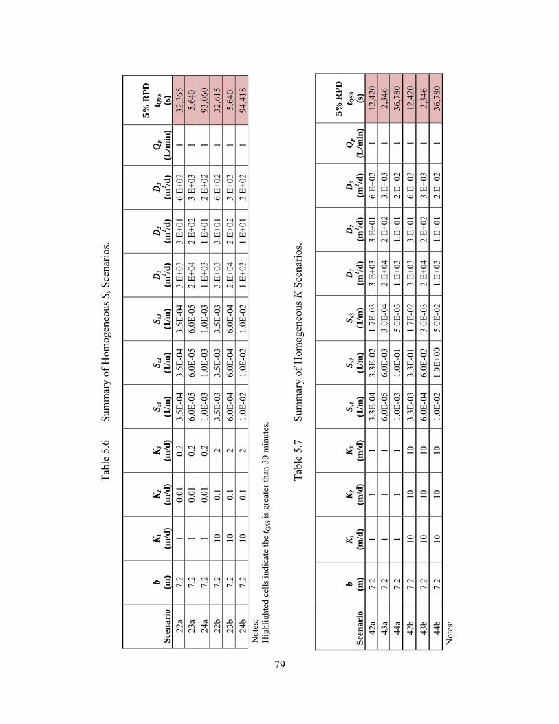
79
Tabl
e 5.
6 Su
mm
ary
of H
omog
eneo
us S
s Sce
nario
s.
Scen
ario
b (m
) K
1 (m
/d)
K2
(m/d
) K
3 (m
/d)
S s1
(1/m
) S s
2 (1
/m)
S s3
(1/m
) D
1 (m
2 /d)
D2
(m2 /d
) D
3 (m
2 /d)
Qp
(L/m
in)
5% R
PD
t QSS
(s
) 22
a 7.
2 1
0.01
0.
2 3.
5E-0
4 3.
5E-0
4 3.
5E-0
4 3.
E+03
3.
E+01
6.
E+02
1
32,3
65
23a
7.2
1 0.
01
0.2
6.0E
-05
6.0E
-05
6.0E
-05
2.E+
04
2.E+
02
3.E+
03
1 5,
640
24a
7.2
1 0.
01
0.2
1.0E
-03
1.0E
-03
1.0E
-03
1.E+
03
1.E+
01
2.E+
02
1 93
,060
22
b 7.
2 10
0.
1 2
3.5E
-03
3.5E
-03
3.5E
-03
3.E+
03
3.E+
01
6.E+
02
1 32
,615
23
b 7.
2 10
0.
1 2
6.0E
-04
6.0E
-04
6.0E
-04
2.E+
04
2.E+
02
3.E+
03
1 5,
640
24b
7.2
10
0.1
2 1.
0E-0
2 1.
0E-0
2 1.
0E-0
2 1.
E+03
1.
E+01
2.
E+02
1
94,4
18
Not
es:
Hig
hlig
hted
cel
ls in
dica
te th
e t Q
SS is
gre
ater
than
30
min
utes
.
Tabl
e 5.
7 Su
mm
ary
of H
omog
eneo
us K
Sce
nario
s.
Scen
ario
b (m
) K
1 (m
/d)
K2
(m/d
) K
3 (m
/d)
S s1
(1/m
) S s
2 (1
/m)
S s3
(1/m
) D
1 (m
2 /d)
D2
(m2 /d
) D
3 (m
2 /d)
Qp
(L/m
in)
5% R
PD
t QSS
(s
) 42
a 7.
2 1
1 1
3.3E
-04
3.3E
-02
1.7E
-03
3.E+
03
3.E+
01
6.E+
02
1 12
,420
43
a 7.
2 1
1 1
6.0E
-05
6.0E
-03
3.0E
-04
2.E+
04
2.E+
02
3.E+
03
1 2,
346
44a
7.2
1 1
1 1.
0E-0
3 1.
0E-0
1 5.
0E-0
3 1.
E+03
1.
E+01
2.
E+02
1
36,7
80
42b
7.2
10
10
10
3.3E
-03
3.3E
-01
1.7E
-02
3.E+
03
3.E+
01
6.E+
02
1 12
,420
43
b 7.
2 10
10
10
6.
0E-0
4 6.
0E-0
2 3.
0E-0
3 2.
E+04
2.
E+02
3.
E+03
1
2,34
6 44
b 7.
2 10
10
10
1.
0E-0
2 1.
0E+0
0 5.
0E-0
2 1.
E+03
1.
E+01
2.
E+02
1
36,7
80
Not
es:

80
Tabl
e 5.
8 Su
mm
ary
of H
omog
eneo
us D
Sce
nario
s.
Scen
ario
b (m
) K
1 (m
/d)
K2
(m/d
) K
3 (m
/d)
S s1
(1/m
) S s
2 (1
/m)
S s3
(1/m
) D
1 (m
2 /d)
D2
(m2 /d
) D
3 (m
2 /d)
Qp
(L/m
in)
5% R
PD
t QSS
(s
) 45
7.
2 1
0.01
0.
2 1.
0E-0
3 1.
0E-0
5 2.
0E-0
4 1.
E+03
1.
E+03
1.
E+03
1
0.06
3 46
7.
2 1
0.01
0.
2 2.
0E-0
4 2.
0E-0
6 4.
0E-0
5 5.
E+03
5.
E+03
5.
E+03
1
0.00
7 47
7.
2 1
0.01
0.
2 2.
0E-0
3 2.
0E-0
5 4.
0E-0
4 5.
E+02
5.
E+02
5.
E+02
1
0.25
5 N
otes
: H
ighl
ight
ed c
ells
indi
cate
the
t QSS
is g
reat
er th
an 3
0 m
inut
es.

81
The effect of varying Ss across layers versus varying K across layers can be seen
in Figures 5.20 and 5.21. In Figure 5.20, K is variable and Ss is constant. As can be seen,
the flows from the high-K layer are initially smaller than their quasi-steady-state values
and conversely, the flows from the lower-K layers are initially greater than their quasi-
steady-state values.
Figure 5.20 Layer flow by depth for Scenario 15.
In Figure 5.21, Ss is variable and K is constant. Here, the flows from the high-D
layers are initially smaller than their quasi-steady-state values and conversely, the flow
from the low-D layer is initially greater than their quasi-steady-state values. These layer
flows are initially discrete values and behave more like a continuous function as they
approach steady-state. As expected, the flows for the homogeneous K scenario
0.0
0.5
1.0
1.5
2.0
2.5
3.0
3.5
4.00.00 0.02 0.04 0.06 0.08 0.10
Dep
th (m
)
Layer Flow (L/min)
t=0.001 st=1,049 st=9,733 s
K=0.2 m/d
K=0.01 m/d
K=1 m/d

82
equilibrate to the same value, with early time differences in behavior driven by
differences in D or Ss.
Figure 5.21 Layer flow by depth for Scenario 42a.
Anisotropy Effects
It is common for aquifers to exhibit directional differences in K, or anisotropy.
To determine the effects of anisotropy on the time for hydraulic gradients at the well to
attain quasi-steady-state, the system described by Scenario 27 was analyzed for
anisotropy ratios (Kz/Kr) ranging from 0.1 to 1.5 (Scenarios 27 and 48 through 52).
These scenarios and their results are summarized in Table 5.9 and Figure 5.22.
0.0
1.0
2.0
3.0
4.0
5.0
6.0
7.0
0.00 0.02 0.04 0.06 0.08 0.10
Dept
h (m
)
Layer Flow (L/min)
t=131 s
t-1,048 s
t=12,458 s
Layer 3K=1 m/dD=3.E+03 m2/d
Layer 2K=1 m/dD=3.E+01 m2/d
Layer 1K=1 m/dD=6.E+02 m2/d

83
Figure 5.22 Time to attain quasi-steady-state as a function of anisotropy ratio for Scenario 27 and Scenarios 48-52.
The results of the anisotropy analysis imply that as the vertical K of the layers is
increased, the amount of crossflow at early times increases, resulting in a smaller time to
quasi-steady-state. This behavior is analogous to that described by Katz and Tek [1962]
who found that the upper limit for crossflow occurs when the vertical hydraulic
conductivity (Kz) approaches infinity compared to the horizontal hydraulic conductivity
(Kr). In other words, as the vertical hydraulic conductivity (Kz) increases relative to the
horizontal hydraulic conductivity (Kr), resistance to crossflow decreases and the time
over which vertical flow significantly affects the overall system behavior decreases.
t = 336.77α-0.906
R² = 1
0.0E+00
5.0E+02
1.0E+03
1.5E+03
2.0E+03
2.5E+03
3.0E+03
0.0 0.5 1.0 1.5 2.0
Tim
e to
Qua
si-S
teady
-Sta
te (s
)
Anisotropy Ratio, α
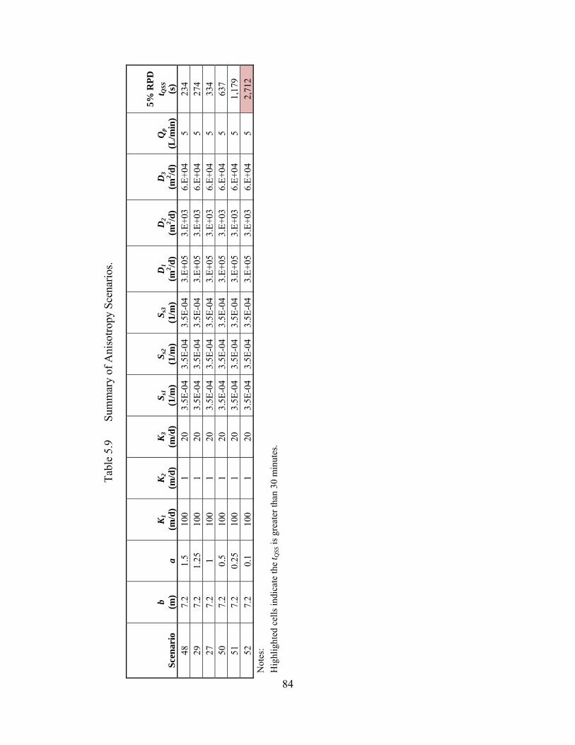
84
Tabl
e 5.
9 Su
mm
ary
of A
niso
tropy
Sce
nario
s.
Scen
ario
b (m
) a
K1
(m/d
) K
2 (m
/d)
K3
(m/d
) S s
1 (1
/m)
S s2
(1/m
) S s
3 (1
/m)
D1
(m2 /d
) D
2 (m
2 /d)
D3
(m2 /d
) Q
p (L
/min
)
5% R
PD
t QSS
(s
) 48
7.
2 1.
5 10
0 1
20
3.5E
-04
3.5E
-04
3.5E
-04
3.E+
05
3.E+
03
6.E+
04
5 23
4 29
7.
2 1.
25
100
1 20
3.
5E-0
4 3.
5E-0
4 3.
5E-0
4 3.
E+05
3.
E+03
6.
E+04
5
274
27
7.2
1 10
0 1
20
3.5E
-04
3.5E
-04
3.5E
-04
3.E+
05
3.E+
03
6.E+
04
5 33
4 50
7.
2 0.
5 10
0 1
20
3.5E
-04
3.5E
-04
3.5E
-04
3.E+
05
3.E+
03
6.E+
04
5 63
7 51
7.
2 0.
25
100
1 20
3.
5E-0
4 3.
5E-0
4 3.
5E-0
4 3.
E+05
3.
E+03
6.
E+04
5
1,17
9 52
7.
2 0.
1 10
0 1
20
3.5E
-04
3.5E
-04
3.5E
-04
3.E+
05
3.E+
03
6.E+
04
5 2,
712
Not
es:
Hig
hlig
hted
cel
ls in
dica
te th
e t Q
SS is
gre
ater
than
30
min
utes
.

85
CHAPTER 6
INTERPRETATION OF RESULTS
Having examined the influence of key parameters on the hydraulic gradient
response (including layer hydraulic conductivity, layer specific storage, layer
arrangement, layer thickness, and overall system thickness), the effects of these factors
on the determination of layer K from flowmeter tests will now be examined. In addition,
the data from the simulations performed during this study will be evaluated to determine
whether the standard pumping duration of 30 minutes is sufficient for attaining
meaningful results from EBF testing and whether a dimensionless time may be defined
such that it may be applied to different systems and function as a predictive tool for the
time to quasi-steady-state (i.e., provide a guideline for the pumping duration required
prior to taking flowmeter readings). The times to quasi-steady-state for the scenarios
discussed in Chapter 5 are summarized in Table 6.1.
Application of Model Results to EBF Analysis
The general practice when performing flowmeter tests has been to pump the well
for 30 minutes at a low flow rate selected based on professional judgment and the results
of previous studies performed in the vicinity or on similar sediments. Earlier, a
maximum RPD between the gradients at the well of 5% was set forth as a viable
definition of quasi-steady-state. By this definition, many of the scenarios modeled in this
study would not achieve quasi-steady-state in 30 minutes or less; this is the case in 29 of
the 85 scenarios presented in Table 6.1. Knowing this, the next step in assessing early-

86
Tabl
e 6.
1 Su
mm
ary
of T
ime
to Q
uasi
-Ste
ady-
Stat
e fo
r Stu
dy S
cena
rios.
Scen
ario
b (m
) a
K1
(m/d
) K
2 (m
/d)
K3
(m/d
) S s
1 (1
/m)
S s2
(1/m
) S s
3 (1
/m)
Qp
(L/m
in)
Δz
(m)
5% R
PD
t QSS
(s
) Q
1 0.
9 1
1 0.
01
0.2
3.5E
-04
3.5E
-04
3.5E
-04
0.30
0 0.
30
933
Q2
0.9
1 10
0 0.
01
0.2
3.5E
-04
3.5E
-04
3.5E
-04
0.20
8 0.
30
1,62
3 Q
3a
0.9
1 0.
01
0.00
01
0.00
2 3.
5E-0
4 3.
5E-0
4 3.
5E-0
4 0.
0030
0 0.
30
93,6
00
Q3b
1.
8 1
0.01
0.
0001
0.
002
3.5E
-04
3.5E
-04
3.5E
-04
0.00
600
0.30
33
7,23
2 Q
3c
3.6
1 0.
01
0.00
01
0.00
2 3.
5E-0
4 3.
5E-0
4 3.
5E-0
4 0.
0120
0 0.
30
927,
600
Q3d
7.
2 1
0.01
0.
0001
0.
002
3.5E
-04
3.5E
-04
3.5E
-04
0.02
40
0.30
3,
222,
700
Q3e
14
.4
1 0.
01
0.00
01
0.00
2 3.
5E-0
4 3.
5E-0
4 3.
5E-0
4 0.
0480
0.
60
11,1
33,7
00
Q3f
28
.8
1 0.
01
0.00
01
0.00
2 3.
5E-0
4 3.
5E-0
4 3.
5E-0
4 0.
0960
1.
20
39,8
98,2
00
Q4a
0.
9 1
1 0.
01
0.2
3.5E
-04
3.5E
-04
3.5E
-04
0.30
0 0.
30
933
Q4b
1.
8 1
1 0.
01
0.2
3.5E
-04
3.5E
-04
3.5E
-04
0.60
0 0.
30
2,88
6 Q
4c
3.6
1 1
0.01
0.
2 3.
5E-0
4 3.
5E-0
4 3.
5E-0
4 1.
20
0.30
9,
716
Q4d
7.
2 1
1 0.
01
0.2
3.5E
-04
3.5E
-04
3.5E
-04
2.40
0.
30
32,2
19
Q4e
14
.4
1 1
0.01
0.
2 3.
5E-0
4 3.
5E-0
4 3.
5E-0
4 4.
80
0.60
11
3,30
8 Q
4f
28.8
1
1 0.
01
0.2
3.5E
-04
3.5E
-04
3.5E
-04
9.60
1.
20
398,
857
Q5a
0.
9 1
100
1 20
3.
5E-0
4 3.
5E-0
4 3.
5E-0
4 30
.0
0.30
10
Q
5b
1.8
1 10
0 1
20
3.5E
-04
3.5E
-04
3.5E
-04
60.0
0.
30
29
Q5c
3.
6 1
100
1 20
3.
5E-0
4 3.
5E-0
4 3.
5E-0
4 12
0 0.
30
98
Q5d
7.
2 1
100
1 20
3.
5E-0
4 3.
5E-0
4 3.
5E-0
4 24
0 0.
30
322
Q5e
14
.4
1 10
0 1
20
3.5E
-04
3.5E
-04
3.5E
-04
480
0.60
1,
115
Q5f
28
.8
1 10
0 1
20
3.5E
-04
3.5E
-04
3.5E
-04
960
1.20
3,
990
Q6a
0.
9 1
10,0
00
100
2,00
0 3.
5E-0
4 3.
5E-0
4 3.
5E-0
4 2,
999
0.30
0.
13
Q6b
1.
8 1
10,0
00
100
2,00
0 3.
5E-0
4 3.
5E-0
4 3.
5E-0
4 5,
999
0.30
0.
38
Q6c
3.
6 1
10,0
00
100
2,00
0 3.
5E-0
4 3.
5E-0
4 3.
5E-0
4 11
,997
0.
30
0.96
Q
6d
7.2
1 10
,000
10
0 2,
000
3.5E
-04
3.5E
-04
3.5E
-04
23,9
94
0.30
3.
2 Q
6e
14.4
1
10,0
00
100
2,00
0 3.
5E-0
4 3.
5E-0
4 3.
5E-0
4 47
,989
0.
60
11
Q6f
28
.8
1 10
,000
10
0 2,
000
3.5E
-04
3.5E
-04
3.5E
-04
95,9
77
1.20
40

87
Tabl
e 6.
1 Su
mm
ary
of T
ime
to Q
uasi
-Ste
ady-
Stat
e fo
r Stu
dy S
cena
rios,
cont
inue
d.
Scen
ario
b (m
) a
K1
(m/d
) K
2 (m
/d)
K3
(m/d
) S s
1 (1
/m)
S s2
(1/m
) S s
3 (1
/m)
Qp
(L/m
in)
Δz
(m)
5% R
PD
t QSS
(s
) Q
7a
0.9
1 1
0.2
0.01
3.
5E-0
4 3.
5E-0
4 3.
5E-0
4 0.
300
0.30
99
3 Q
7b
0.9
1 0.
2 1
0.01
3.
5E-0
4 3.
5E-0
4 3.
5E-0
4 0.
300
0.30
90
3 Q
7c
28.8
1
1 0.
2 0.
01
3.5E
-04
3.5E
-04
3.5E
-04
9.60
1.
20
434,
094
Q7d
28
.8
1 0.
2 1
0.01
3.
5E-0
4 3.
5E-0
4 3.
5E-0
4 9.
60
1.20
43
3,96
5 1
0.9
1 1
0.01
0.
2 3.
5E-0
4 3.
5E-0
4 3.
5E-0
4 0.
1 0.
3 91
6 2
0.9
1 1
0.01
0.
2 6.
0E-0
5 6.
0E-0
5 6.
0E-0
5 0.
1 0.
3 15
7 3
0.9
1 1
0.01
0.
2 1.
0E-0
3 1.
0E-0
3 1.
0E-0
3 0.
1 0.
3 2,
613
4 0.
9 1
1 0.
01
0.2
3.5E
-04
3.5E
-04
3.5E
-04
0.6
0.3
916
5 0.
9 1
100
1 20
3.
5E-0
4 3.
5E-0
4 3.
5E-0
4 5
0.3
9.09
6
0.9
1 10
,000
10
0 2,
000
3.5E
-04
3.5E
-04
3.5E
-04
5 0.
3 0.
127
7 1.
8 1
1 0.
01
0.2
3.5E
-04
3.5E
-04
3.5E
-04
0.3
0.3
2,83
6 7a
1.
8 1
1 0.
01
0.2
3.5E
-04
3.5E
-04
3.5E
-04
0.3
0.3
1,47
3 8
1.8
1 1
0.01
0.
2 6.
0E-0
5 6.
0E-0
5 6.
0E-0
5 0.
3 0.
3 51
3 9
1.8
1 1
0.01
0.
2 1.
0E-0
3 1.
0E-0
3 1.
0E-0
3 0.
3 0.
3 8,
220
10
1.8
1 1
0.01
0.
2 3.
5E-0
4 3.
5E-0
4 3.
5E-0
4 5
0.3
2,85
3 11
1.
8 1
100
1 20
3.
5E-0
4 3.
5E-0
4 3.
5E-0
4 0.
5 0.
3 36
.4
12
1.8
1 10
0 1
20
3.5E
-04
3.5E
-04
3.5E
-04
5 0.
3 33
.9
13
1.8
1 10
0 1
20
3.5E
-04
3.5E
-04
3.5E
-04
40
0.3
36.4
14
1.
8 1
10,0
00
100
2,00
0 3.
5E-0
4 3.
5E-0
4 3.
5E-0
4 5
0.3
0.35
1 15
3.
6 1
1 0.
01
0.2
3.5E
-04
3.5E
-04
3.5E
-04
0.5
0.3
9,73
3 16
3.
6 1
1 0.
01
0.2
6.0E
-05
6.0E
-05
6.0E
-05
0.5
0.3
1,62
3 17
3.
6 1
1 0.
01
0.2
1.0E
-03
1.0E
-03
1.0E
-03
0.5
0.3
27,3
30
18
3.6
1 1
0.01
0.
2 3.
5E-0
4 3.
5E-0
4 3.
5E-0
4 5
0.3
9,27
8 18
a 3.
6 1
1 0.
01
0.2
3.5E
-04
3.5E
-04
3.5E
-04
5 0.
3 2,
206
19
3.6
1 1
0.01
0.
2 3.
5E-0
4 3.
5E-0
4 3.
5E-0
4 10
0.
3 9,
300
20
3.6
1 10
0 1
20
3.5E
-04
3.5E
-04
3.5E
-04
5 0.
3 98
.3
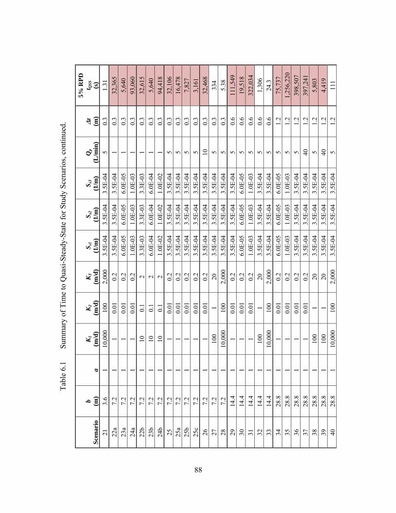
88
Tabl
e 6.
1 Su
mm
ary
of T
ime
to Q
uasi
-Ste
ady-
Stat
e fo
r Stu
dy S
cena
rios,
cont
inue
d.
Scen
ario
b (m
) a
K1
(m/d
) K
2 (m
/d)
K3
(m/d
) S s
1 (1
/m)
S s2
(1/m
) S s
3 (1
/m)
Qp
(L/m
in)
Δz
(m)
5% R
PD
t QSS
(s
) 21
3.
6 1
10,0
00
100
2,00
0 3.
5E-0
4 3.
5E-0
4 3.
5E-0
4 5
0.3
1.31
22
a 7.
2 1
1 0.
01
0.2
3.5E
-04
3.5E
-04
3.5E
-04
1 0.
3 32
,365
23
a 7.
2 1
1 0.
01
0.2
6.0E
-05
6.0E
-05
6.0E
-05
1 0.
3 5,
640
24a
7.2
1 1
0.01
0.
2 1.
0E-0
3 1.
0E-0
3 1.
0E-0
3 1
0.3
93,0
60
22b
7.2
1 10
0.
1 2
3.3E
-03
3.3E
-03
3.3E
-03
1 0.
3 32
,615
23
b 7.
2 1
10
0.1
2 6.
0E-0
4 6.
0E-0
4 6.
0E-0
4 1
0.3
5,64
0 24
b 7.
2 1
10
0.1
2 1.
0E-0
2 1.
0E-0
2 1.
0E-0
2 1
0.3
94,4
18
25
7.2
1 1
0.01
0.
2 3.
5E-0
4 3.
5E-0
4 3.
5E-0
4 5
0.3
32,1
06
25a
7.2
1 1
0.01
0.
2 3.
5E-0
4 3.
5E-0
4 3.
5E-0
4 5
0.3
16,4
78
25b
7.2
1 1
0.01
0.
2 3.
5E-0
4 3.
5E-0
4 3.
5E-0
4 5
0.3
7,82
7 25
c 7.
2 1
1 0.
01
0.2
3.5E
-04
3.5E
-04
3.5E
-04
5 0.
3 3,
161
26
7.2
1 1
0.01
0.
2 3.
5E-0
4 3.
5E-0
4 3.
5E-0
4 10
0.
3 32
,468
27
7.
2 1
100
1 20
3.
5E-0
4 3.
5E-0
4 3.
5E-0
4 5
0.3
334
28
7.2
1 10
,000
10
0 2,
000
3.5E
-04
3.5E
-04
3.5E
-04
5 0.
3 5.
38
29
14.4
1
1 0.
01
0.2
3.5E
-04
3.5E
-04
3.5E
-04
5 0.
6 11
1,54
9 30
14
.4
1 1
0.01
0.
2 6.
0E-0
5 6.
0E-0
5 6.
0E-0
5 5
0.6
19,5
18
31
14.4
1
1 0.
01
0.2
1.0E
-03
1.0E
-03
1.0E
-03
5 0.
6 32
2,03
4 32
14
.4
1 10
0 1
20
3.5E
-04
3.5E
-04
3.5E
-04
5 0.
6 1,
306
33
14.4
1
10,0
00
100
2,00
0 3.
5E-0
4 3.
5E-0
4 3.
5E-0
4 5
0.6
24.3
34
28
.8
1 1
0.01
0.
2 6.
0E-0
5 6.
0E-0
5 6.
0E-0
5 5
1.2
75,7
37
35
28.8
1
1 0.
01
0.2
1.0E
-03
1.0E
-03
1.0E
-03
5 1.
2 1,
256,
220
36
28.8
1
1 0.
01
0.2
3.5E
-04
3.5E
-04
3.5E
-04
5 1.
2 39
8,50
7 37
28
.8
1 1
0.01
0.
2 3.
5E-0
4 3.
5E-0
4 3.
5E-0
4 40
1.
2 39
7,24
1 38
28
.8
1 10
0 1
20
3.5E
-04
3.5E
-04
3.5E
-04
5 1.
2 5,
803
39
28.8
1
100
1 20
3.
5E-0
4 3.
5E-0
4 3.
5E-0
4 40
1.
2 4,
419
40
28.8
1
10,0
00
100
2,00
0 3.
5E-0
4 3.
5E-0
4 3.
5E-0
4 5
1.2
111
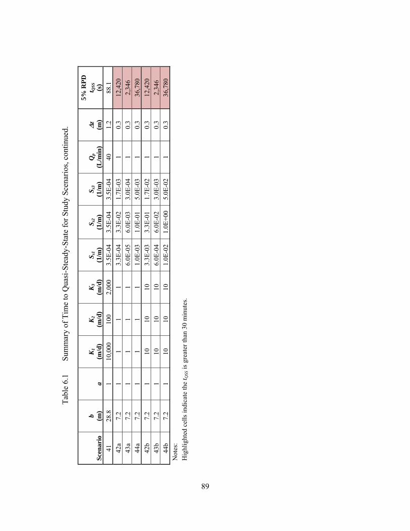
89
Tabl
e 6.
1 Su
mm
ary
of T
ime
to Q
uasi
-Ste
ady-
Stat
e fo
r Stu
dy S
cena
rios,
cont
inue
d.
Scen
ario
b (m
) a
K1
(m/d
) K
2 (m
/d)
K3
(m/d
) S s
1 (1
/m)
S s2
(1/m
) S s
3 (1
/m)
Qp
(L/m
in)
Δz
(m)
5% R
PD
t QSS
(s
) 41
28
.8
1 10
,000
10
0 2,
000
3.5E
-04
3.5E
-04
3.5E
-04
40
1.2
88.1
42
a 7.
2 1
1 1
1 3.
3E-0
4 3.
3E-0
2 1.
7E-0
3 1
0.3
12,4
20
43a
7.2
1 1
1 1
6.0E
-05
6.0E
-03
3.0E
-04
1 0.
3 2,
346
44a
7.2
1 1
1 1
1.0E
-03
1.0E
-01
5.0E
-03
1 0.
3 36
,780
42
b 7.
2 1
10
10
10
3.3E
-03
3.3E
-01
1.7E
-02
1 0.
3 12
,420
43
b 7.
2 1
10
10
10
6.0E
-04
6.0E
-02
3.0E
-03
1 0.
3 2,
346
44b
7.2
1 10
10
10
1.
0E-0
2 1.
0E+0
0 5.
0E-0
2 1
0.3
36,7
80
Not
es:
Hig
hlig
hted
cel
ls in
dica
te th
e t Q
SS is
gre
ater
than
30
min
utes
.

90
time flow behavior toward a well under pumping conditions is determining the impact on
the calculated K values of taking flowmeter measurements prior to the time when the
maximum RPD between the gradients at the well is 5% or less. To evaluate this effect,
Eqn. 2-3 may be modified such that the ambient flow is removed from the equation to
obtain:
bQzQ
KK
P
iii
// ΔΔ
=><
(6-1)
Using this equation in conjunction with the EBF range of measurement of 40
mL/min (0.05 m3/d) to 40 L/min (57.6 m3/d) as well as the device readout truncation, it is
possible to calculate the K for each model layer at each time step. The model directly
outputs the differential flow for each layer into the well (ΔQj). The cumulative flow at
each successive Δz is calculated based on the raw interval flow contributions. The
truncation from the readout device is then applied to the cumulative flow at each interval.
The cumulative flow at each interval is then compared to the upper and lower
measurement limits of the EBF. It is at this point that the flowmeter analysis is applied,
using Eqn. 6-1 to determine the layer-K values.
Flowmeter tests using the EBF are conducted by measuring the cumulative flow
into or out of the well as the device is raised along the well-face. This implies that if
layers or measurement intervals have flow contributions below the device detection limit
or the display capabilities, these flows will be incorporated into the next interval
measurement where the flow is large enough to be detected. By definition, this will
result in a layer with a flow contribution below the detection limit having the same device
91
reading as the previous interval, whereas the measurement for the interval next reflecting
an increase in the cumulative flow will be greater than the true contribution for that
interval. In evaluating the scenarios used in the evaluation of flowmeter analysis, the
cumulative flow at each interval was compared to the device range of measurements,
with values below the lower detection limit set to zero. Additionally, the flow readings
from the EBF are truncated to two significant figures after the decimal to reflect the
readout capacities of the device.
The K values obtained using Eqn. 6-1 can then be compared to the input layer K
values to determine subjectively when the system has equilibrated sufficiently to yield
calculated results representative of the input values, even though these calculated values
may not be equal to the input K values. This process is, as noted, partly subjective rather
than fully quantitative, but in general the times were selected such that when rounded, the
K values equaled the input values. As an example, the calculated K values for the
subjective time to quasi-steady-state from Scenario 15 are included in Table 6.2. In this
example, the calculated K values differ slightly from the input K values; however, the
difference is slight and is unlikely to result in any qualitative differences in assessment of
the aquifer behavior.

92
Table 6.2 Summary of Input and Calculated K values at the Subjective Quasi-Steady-State for Scenario 15
Layer Layer K
(m/d) Depth, z
(m) Input K (m/d)
Calculated K (m/d)
Average Calculated
K (m/d)
1 1
3.45 1.00 0.97
0.97 3.15 1.00 0.97 2.85 1.00 0.97 2.55 1.00 0.98
2 0.01
2.25 0.01 0.010
0.013 1.95 0.01 0.010 1.65 0.01 0.010 1.35 0.01 0.021
3 0.2
1.05 0.20 0.22
0.23 0.75 0.20 0.23 0.45 0.20 0.23 0.15 0.20 0.22
93
The subjective times to quasi-steady-state for Scenarios Q1-Q7 and 1-44 are
included in Table 6.3. As can be seen in Table 6.3, the subjective times to quasi-steady-
state are smaller, often significantly, than those for when the RPD between the gradients
at the well is approximately 5%. Corresponding to these shorter times, the RPD between
the gradients at the well at the subjective times to quasi-steady-state are significantly
larger than 5%, ranging from 8% to 158% with an average of 64% (Table 6.3). This is an
important finding because it demonstrates that it is possible to obtain representative K
values for an aquifer during the period when flow into the well (which is directly
proportional to the gradient at the well) is still transient. Using the subjective time to
quasi-steady-state, 65 of the 68 scenarios summarized in Table 6.3 attained quasi-steady-
state prior to 30 minutes pumping duration.
The calculated K values for the three scenarios not considered to have
subjectively attained quasi-steady-state before 30 minutes (Scenarios Q4e, 29, and 31)
were examined at the output time closest to and less than 30 minutes (Table 6.4). As can
be seen, although the output was not subjectively considered to have attained quasi-
steady-state at the times nearest 30 minutes (t=1,049 s for Scenarios Q4e and 29, and
t=1,704 s for Scenario 31) as not all layer calculated K’s rounded to the corresponding
input value, assessment of these results show that the individual grid-layer K results as
well as the average K results over each layer are consistent with the input values.
Furthermore, the differences seen at these times between the calculated and input K-
values are not considered significant and would likely not adversely affect any further
efforts based on this dataset.

94
Tabl
e 6.
3 Su
mm
ary
of S
ubje
ctiv
e Ti
mes
to Q
uasi
-Ste
ady-
Stat
e.
Scen
ario
b (m
) K
1 (m
/d)
K2
(m/d
) K
3 (m
/d)
S s1
(1/m
) S s
2 (1
/m)
S s3
(1/m
) Q
p (L
/min
)
5% R
PD
t QSS
(s
)
Subj
ectiv
e t Q
SS
(s)
RPD
at
Subj
ectiv
e t Q
SS
Q1
0.9
1 0.
01
0.2
3.5E
-04
3.5E
-04
3.5E
-04
0.30
0 93
3 18
79
%
Q2
0.9
100
0.01
0.
2 3.
5E-0
4 3.
5E-0
4 3.
5E-0
4 0.
208
1,62
3 8.
2 13
4%
Q3a
0.
9 0.
01
0.00
01
0.00
2 3.
5E-0
4 3.
5E-0
4 3.
5E-0
4 0.
0030
0 93
,600
N
A
NA
Q
3b
1.8
0.01
0.
0001
0.
002
3.5E
-04
3.5E
-04
3.5E
-04
0.00
600
337,
232
NA
N
A
Q3c
3.
6 0.
01
0.00
01
0.00
2 3.
5E-0
4 3.
5E-0
4 3.
5E-0
4 0.
0120
0 92
7,60
0 N
A
NA
Q
3d
7.2
0.01
0.
0001
0.
002
3.5E
-04
3.5E
-04
3.5E
-04
0.02
40
3,22
2,70
0 N
A
NA
Q
3e
14.4
0.
01
0.00
01
0.00
2 3.
5E-0
4 3.
5E-0
4 3.
5E-0
4 0.
0480
11
,133
,700
N
A
NA
Q
3f
28.8
0.
01
0.00
01
0.00
2 3.
5E-0
4 3.
5E-0
4 3.
5E-0
4 0.
0960
39
,898
,200
N
A
NA
Q
4a
0.9
1 0.
01
0.2
3.5E
-04
3.5E
-04
3.5E
-04
0.30
0 93
3 18
79
%
Q4b
1.
8 1
0.01
0.
2 3.
5E-0
4 3.
5E-0
4 3.
5E-0
4 0.
600
2,88
6 24
6 38
%
Q4c
3.
6 1
0.01
0.
2 3.
5E-0
4 3.
5E-0
4 3.
5E-0
4 1.
20
9,71
6 1,
049
30%
Q
4d
7.2
1 0.
01
0.2
3.5E
-04
3.5E
-04
3.5E
-04
2.40
32
,219
1,
180
46%
Q
4e
14.4
1
0.01
0.
2 3.
5E-0
4 3.
5E-0
4 3.
5E-0
4 4.
80
113,
308
3,60
0 43
%
Q4f
28
.8
1 0.
01
0.2
3.5E
-04
3.5E
-04
3.5E
-04
9.60
39
8,85
7 26
2 66
%
Q5a
0.
9 10
0 1
20
3.5E
-04
3.5E
-04
3.5E
-04
30.0
10
6.
0 8%
Q
5b
1.8
100
1 20
3.
5E-0
4 3.
5E-0
4 3.
5E-0
4 60
.0
29
NA
N
A
Q5c
3.
6 10
0 1
20
3.5E
-04
3.5E
-04
3.5E
-04
120
98
NA
N
A
Q5d
7.
2 10
0 1
20
3.5E
-04
3.5E
-04
3.5E
-04
240
322
NA
N
A
Q5e
14
.4
100
1 20
3.
5E-0
4 3.
5E-0
4 3.
5E-0
4 48
0 1,
115
NA
N
A
Q5f
28
.8
100
1 20
3.
5E-0
4 3.
5E-0
4 3.
5E-0
4 96
0 3,
990
NA
N
A
Q6a
0.
9 10
,000
10
0 2,
000
3.5E
-04
3.5E
-04
3.5E
-04
2,99
9 0.
13
NA
N
A
Q6b
1.
8 10
,000
10
0 2,
000
3.5E
-04
3.5E
-04
3.5E
-04
5,99
9 0.
38
NA
N
A
Q6c
3.
6 10
,000
10
0 2,
000
3.5E
-04
3.5E
-04
3.5E
-04
11,9
97
0.96
N
A
NA
Q
6d
7.2
10,0
00
100
2,00
0 3.
5E-0
4 3.
5E-0
4 3.
5E-0
4 23
,994
3.
2 N
A
NA
Q
6e
14.4
10
,000
10
0 2,
000
3.5E
-04
3.5E
-04
3.5E
-04
47,9
89
11
NA
N
A
Q6f
28
.8
10,0
00
100
2,00
0 3.
5E-0
4 3.
5E-0
4 3.
5E-0
4 95
,977
40
N
A
NA
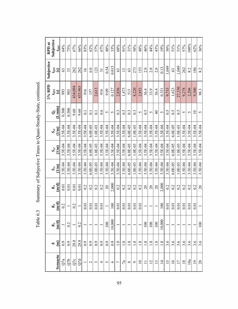
95
Tabl
e 6.
3 Su
mm
ary
of S
ubje
ctiv
e Ti
mes
to Q
uasi
-Ste
ady-
Stat
e, c
ontin
ued.
Scen
ario
b (m
) K
1 (m
/d)
K2
(m/d
) K
3 (m
/d)
S s1
(1/m
) S s
2 (1
/m)
S s3
(1/m
) Q
p (L
/min
)
5% R
PD
t QSS
(s
)
Subj
ectiv
e t Q
SS
(s)
RPD
at
Subj
ectiv
e t Q
SS
Q7a
0.
9 1
0.2
0.01
3.
5E-0
4 3.
5E-0
4 3.
5E-0
4 0.
300
993
63
64%
Q
7b
0.9
0.2
1 0.
01
3.5E
-04
3.5E
-04
3.5E
-04
0.30
0 90
3 33
75
%
Q7c
28
.8
1 0.
2 0.
01
3.5E
-04
3.5E
-04
3.5E
-04
9.60
43
4,09
4 26
2 67
%
Q7d
28
.8
0.2
1 0.
01
3.5E
-04
3.5E
-04
3.5E
-04
9.60
43
3,96
5 26
2 66
%
1 0.
9 1
0.01
0.
2 3.
5E-0
4 3.
5E-0
4 3.
5E-0
4 0.
1 91
6 16
83
%
2 0.
9 1
0.01
0.
2 6.
0E-0
5 6.
0E-0
5 6.
0E-0
5 0.
1 15
7 6.
0 62
%
3 0.
9 1
0.01
0.
2 1.
0E-0
3 1.
0E-0
3 1.
0E-0
3 0.
1 2,
613
123
57%
4
0.9
1 0.
01
0.2
3.5E
-04
3.5E
-04
3.5E
-04
0.6
916
31
67%
5
0.9
100
1 20
3.
5E-0
4 3.
5E-0
4 3.
5E-0
4 5
9.09
0.
54
48%
6
0.9
10,0
00
100
2,00
0 3.
5E-0
4 3.
5E-0
4 3.
5E-0
4 5
0.12
7 0.
015
33%
7
1.8
1 0.
01
0.2
3.5E
-04
3.5E
-04
3.5E
-04
0.3
2,83
6 63
68
%
7a
1.8
1 0.
01
0.2
3.5E
-04
3.5E
-04
3.5E
-04
0.3
1,47
3 13
91
%
8 1.
8 1
0.01
0.
2 6.
0E-0
5 6.
0E-0
5 6.
0E-0
5 0.
3 51
3 63
31
%
9 1.
8 1
0.01
0.
2 1.
0E-0
3 1.
0E-0
3 1.
0E-0
3 0.
3 8,
220
273
58%
10
1.
8 1
0.01
0.
2 3.
5E-0
4 3.
5E-0
4 3.
5E-0
4 5
2,85
3 15
3 48
%
11
1.8
100
1 20
3.
5E-0
4 3.
5E-0
4 3.
5E-0
4 0.
5 36
.4
2.0
46%
12
1.
8 10
0 1
20
3.5E
-04
3.5E
-04
3.5E
-04
5 33
.9
2.0
44%
13
1.
8 10
0 1
20
3.5E
-04
3.5E
-04
3.5E
-04
40
36.4
2.
0 43
%
14
1.8
10,0
00
100
2,00
0 3.
5E-0
4 3.
5E-0
4 3.
5E-0
4 5
0.35
1 0.
13
19%
15
3.
6 1
0.01
0.
2 3.
5E-0
4 3.
5E-0
4 3.
5E-0
4 0.
5 9,
733
1,04
9 30
%
16
3.6
1 0.
01
0.2
6.0E
-05
6.0E
-05
6.0E
-05
0.5
1,62
3 63
51
%
17
3.6
1 0.
01
0.2
1.0E
-03
1.0E
-03
1.0E
-03
0.5
27,3
30
1,04
9 51
%
18
3.6
1 0.
01
0.2
3.5E
-04
3.5E
-04
3.5E
-04
5 9,
278
262
57%
18
a 3.
6 1
0.01
0.
2 3.
5E-0
4 3.
5E-0
4 3.
5E-0
4 5
2,20
6 8.
2 10
0%
19
3.6
1 0.
01
0.2
3.5E
-04
3.5E
-04
3.5E
-04
10
9,30
0 18
6 62
%
20
3.6
100
1 20
3.
5E-0
4 3.
5E-0
4 3.
5E-0
4 5
98.3
8.
2 36
%
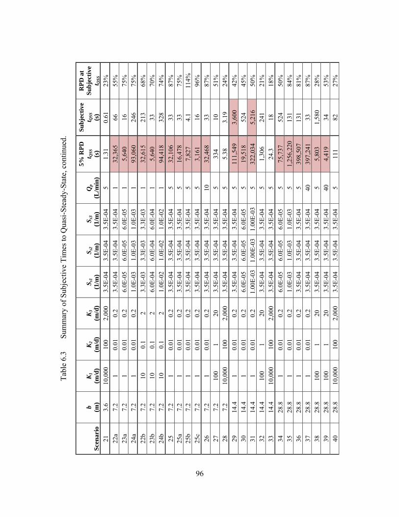
96
Tabl
e 6.
3 Su
mm
ary
of S
ubje
ctiv
e Ti
mes
to Q
uasi
-Ste
ady-
Stat
e, c
ontin
ued.
Scen
ario
b (m
) K
1 (m
/d)
K2
(m/d
) K
3 (m
/d)
S s1
(1/m
) S s
2 (1
/m)
S s3
(1/m
) Q
p (L
/min
)
5% R
PD
t QSS
(s
)
Subj
ectiv
e t Q
SS
(s)
RPD
at
Subj
ectiv
e t Q
SS
21
3.6
10,0
00
100
2,00
0 3.
5E-0
4 3.
5E-0
4 3.
5E-0
4 5
1.31
0.
61
23%
22
a 7.
2 1
0.01
0.
2 3.
5E-0
4 3.
5E-0
4 3.
5E-0
4 1
32,3
65
66
55%
23
a 7.
2 1
0.01
0.
2 6.
0E-0
5 6.
0E-0
5 6.
0E-0
5 1
5,64
0 16
75
%
24a
7.2
1 0.
01
0.2
1.0E
-03
1.0E
-03
1.0E
-03
1 93
,060
24
6 75
%
22b
7.2
10
0.1
2 3.
3E-0
3 3.
3E-0
3 3.
3E-0
3 1
32,6
15
213
68%
23
b 7.
2 10
0.
1 2
6.0E
-04
6.0E
-04
6.0E
-04
1 5,
640
33
70%
24
b 7.
2 10
0.
1 2
1.0E
-02
1.0E
-02
1.0E
-02
1 94
,418
32
8 74
%
25
7.2
1 0.
01
0.2
3.5E
-04
3.5E
-04
3.5E
-04
5 32
,106
33
87
%
25a
7.2
1 0.
01
0.2
3.5E
-04
3.5E
-04
3.5E
-04
5 16
,478
33
75
%
25b
7.2
1 0.
01
0.2
3.5E
-04
3.5E
-04
3.5E
-04
5 7,
827
4.1
114%
25
c 7.
2 1
0.01
0.
2 3.
5E-0
4 3.
5E-0
4 3.
5E-0
4 5
3,16
1 16
96
%
26
7.2
1 0.
01
0.2
3.5E
-04
3.5E
-04
3.5E
-04
10
32,4
68
33
87%
27
7.
2 10
0 1
20
3.5E
-04
3.5E
-04
3.5E
-04
5 33
4 10
51
%
28
7.2
10,0
00
100
2,00
0 3.
5E-0
4 3.
5E-0
4 3.
5E-0
4 5
5.38
3.
19
24%
29
14
.4
1 0.
01
0.2
3.5E
-04
3.5E
-04
3.5E
-04
5 11
1,54
9 3,
600
42%
30
14
.4
1 0.
01
0.2
6.0E
-05
6.0E
-05
6.0E
-05
5 19
,518
52
4 45
%
31
14.4
1
0.01
0.
2 1.
00E-
03
1.00
E-03
1.
00E-
03
5 32
2,03
4 5,
216
50%
32
14
.4
100
1 20
3.
5E-0
4 3.
5E-0
4 3.
5E-0
4 5
1,30
6 24
1 21
%
33
14.4
10
,000
10
0 2,
000
3.5E
-04
3.5E
-04
3.5E
-04
5 24
.3
18
18%
34
28
.8
1 0.
01
0.2
6.0E
-05
6.0E
-05
6.0E
-05
5 75
,737
52
4 50
%
35
28.8
1
0.01
0.
2 1.
0E-0
3 1.
0E-0
3 1.
0E-0
3 5
1,25
6,22
0 13
1 84
%
36
28.8
1
0.01
0.
2 3.
5E-0
4 3.
5E-0
4 3.
5E-0
4 5
398,
507
131
81%
37
28
.8
1 0.
01
0.2
3.5E
-04
3.5E
-04
3.5E
-04
40
397,
241
33
87%
38
28
.8
100
1 20
3.
5E-0
4 3.
5E-0
4 3.
5E-0
4 5
5,80
3 1,
580
28%
39
28
.8
100
1 20
3.
5E-0
4 3.
5E-0
4 3.
5E-0
4 40
4,
419
34
53%
40
28
.8
10,0
00
100
2,00
0 3.
5E-0
4 3.
5E-0
4 3.
5E-0
4 5
111
82
27%
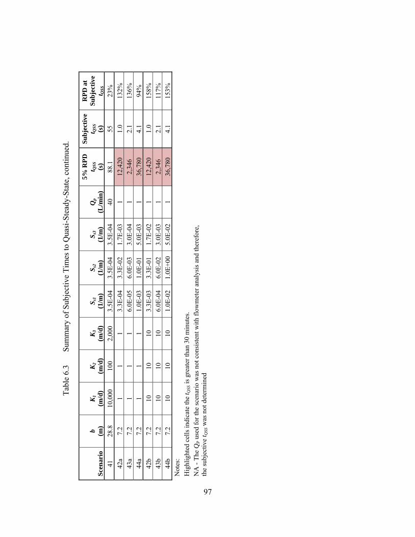
97
Tabl
e 6.
3 Su
mm
ary
of S
ubje
ctiv
e Ti
mes
to Q
uasi
-Ste
ady-
Stat
e, c
ontin
ued.
Scen
ario
b (m
) K
1 (m
/d)
K2
(m/d
) K
3 (m
/d)
S s1
(1/m
) S s
2 (1
/m)
S s3
(1/m
) Q
p (L
/min
)
5% R
PD
t QSS
(s
)
Subj
ectiv
e t Q
SS
(s)
RPD
at
Subj
ectiv
e t Q
SS
41
28.8
10
,000
10
0 2,
000
3.5E
-04
3.5E
-04
3.5E
-04
40
88.1
55
23
%
42a
7.2
1 1
1 3.
3E-0
4 3.
3E-0
2 1.
7E-0
3 1
12,4
20
1.0
132%
43
a 7.
2 1
1 1
6.0E
-05
6.0E
-03
3.0E
-04
1 2,
346
2.1
136%
44
a 7.
2 1
1 1
1.0E
-03
1.0E
-01
5.0E
-03
1 36
,780
4.
1 94
%
42b
7.2
10
10
10
3.3E
-03
3.3E
-01
1.7E
-02
1 12
,420
1.
0 15
8%
43b
7.2
10
10
10
6.0E
-04
6.0E
-02
3.0E
-03
1 2,
346
2.1
117%
44
b 7.
2 10
10
10
1.
0E-0
2 1.
0E+0
0 5.
0E-0
2 1
36,7
80
4.1
153%
N
otes
: H
ighl
ight
ed c
ells
indi
cate
the
t QSS
is g
reat
er th
an 3
0 m
inut
es.
NA
- Th
e Q
P use
d fo
r the
scen
ario
was
not
con
sist
ent w
ith fl
owm
eter
ana
lysi
s and
ther
efor
e,
the
subj
ectiv
e t Q
SS w
as n
ot d
eter
min
ed
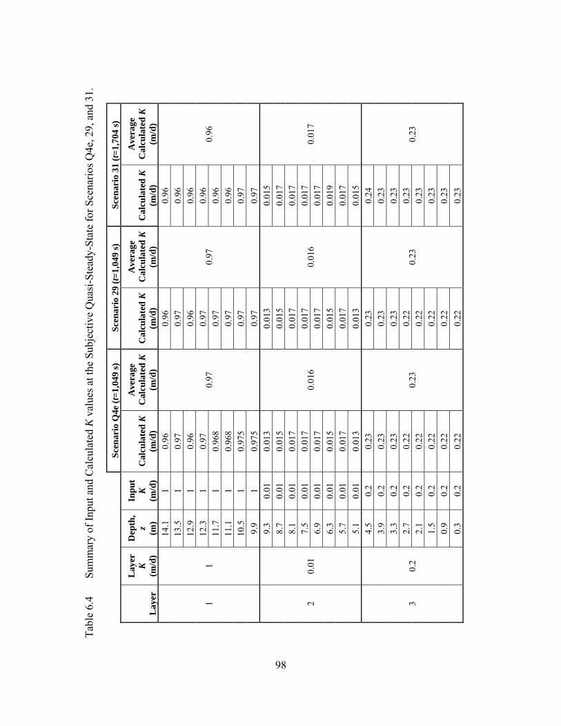
98
Tabl
e 6.
4 Su
mm
ary
of In
put a
nd C
alcu
late
d K
val
ues a
t the
Sub
ject
ive
Qua
si-S
tead
y-St
ate
for S
cena
rios Q
4e, 2
9, a
nd 3
1.
Scen
ario
Q4e
(t=1
,049
s)
Scen
ario
29
(t=1,
049
s)
Scen
ario
31
(t=1,
704
s)
Lay
er
Lay
er
K
(m/d
)
Dep
th,
z (m)
Inpu
t K
(m
/d)
Cal
cula
ted
K(m
/d)
Ave
rage
C
alcu
late
d K
(m/d
) C
alcu
late
d K
(m
/d)
Ave
rage
C
alcu
late
d K
(m/d
) C
alcu
late
d K
(m/d
)
Ave
rage
C
alcu
late
d K
(m/d
)
1 1
14.1
1
0.96
0.97
0.96
0.97
0.96
0.96
13.5
1
0.97
0.
97
0.96
12
.9
1 0.
96
0.96
0.
96
12.3
1
0.97
0.
97
0.96
11
.7
1 0.
968
0.97
0.
96
11.1
1
0.96
8 0.
97
0.96
10
.5
1 0.
975
0.97
0.
97
9.9
1 0.
975
0.97
0.
97
2 0.
01
9.3
0.01
0.
013
0.01
6
0.01
3
0.01
6
0.01
5
0.01
7
8.7
0.01
0.
015
0.01
5 0.
017
8.1
0.01
0.
017
0.01
7 0.
017
7.5
0.01
0.
017
0.01
7 0.
017
6.9
0.01
0.
017
0.01
7 0.
017
6.3
0.01
0.
015
0.01
5 0.
019
5.7
0.01
0.
017
0.01
7 0.
017
5.1
0.01
0.
013
0.01
3 0.
015
3 0.
2
4.5
0.2
0.23
0.23
0.23
0.23
0.24
0.23
3.9
0.2
0.23
0.
23
0.23
3.
3 0.
2 0.
23
0.23
0.
23
2.7
0.2
0.22
0.
22
0.23
2.
1 0.
2 0.
22
0.22
0.
23
1.5
0.2
0.22
0.
22
0.23
0.
9 0.
2 0.
22
0.22
0.
23
0.3
0.2
0.22
0.
22
0.23

99
The finding that it is possible to obtain representative K values for an aquifer
during the period when flow into the well is still transient is, on the surface, contradictory
to the findings of Ruud and Kabala [1996], who concluded that systems may be
persistently transient for individual layer flows. This study has found results analogous
to those of Ruud and Kabala [1996] in that the layer flows in many systems in this study
required longer than the tD of 1,000 defined by Javandel and Witherspoon [1969] for
individual layer flows to equilibrate. As will be demonstrated in the next discussion
topic, the use of this particular dimensionless time for the prediction of quasi-steady-state
is questionable; however, it is possible to evaluate the Ruud and Kabala [1996] results
with respect to the flowmeter methodology described above.
Figure 6.1 and Table 6.5 includes the input K values and individual layer flow
values from the Ruud and Kabala [1996] figure (Figure 6.1) as well as calculated K
values using the flowmeter methodology described earlier in this Chapter for the different
times shown in the figure. As can be seen from the calculated K values in Table 6.5, the
calculated flow rates for the lower-K layer are approximately an order of magnitude
different from the input value; however, by t=720 s, the calculated K value for this same
layer is now just a factor of two greater than the input value. For the purposes of most
applications, the real-world difference between 0.073 m/d (calculated value at t=720 s)
and 0.035 m/d (input value) is not significant. Furthermore, the calculated K of 3.4 m/d
for the dominant layer in the system (i.e., the high-K layer, with respect to transport or
productivity) is consistent with the input value (3.5 m/d) for even the earliest time
included (90 s).

100
Figure 6.1 Figure 5 from Ruud and Kabala [1996].

101
Tabl
e 6.
5 Su
mm
ary
of In
put a
nd C
alcu
late
d K
val
ues f
or th
e R
esul
ts fr
om R
uud
and
Kab
ala
[199
6] F
igur
e 5
t=90
s t=
720
s t=
10,8
00 s
Lay
er
Lay
er
K
(m/d
)
Dep
th,
z (m)
Inpu
t K
(m
/d)
ΔQ
(m3 /d
)
Cal
cula
ted
K
(m/d
)
Ave
rage
C
alcu
late
d K
(m
/d)
ΔQ
(m3 /d
)
Cal
cula
ted
K
(m/d
)
Ave
rage
C
alcu
late
d K
(m
/d)
ΔQ
(m3 /d
)
Cal
cula
ted
K
(m/d
)
Ave
rage
C
alcu
late
d K
(m
/d)
1 4
0.5
3.5
23
3.4
3.4
23
3.4
3.4
23
3.4
3.4
1.5
3.5
23
3.4
23
3.4
23
3.4
2.5
3.5
23
3.4
23
3.4
23
3.4
3.5
3.5
23
3.4
23
3.4
23
3.4
4.5
3.5
23
3.4
23
3.4
23
3.4
2 0.
035
5.5
0.03
5 0.
74
0.1
0.11
0.50
0.
07
0.07
3
0.36
0.
05
0.05
2
6.5
0.03
5 0.
74
0.1
0.50
0.
07
0.36
0.
05
7.5
0.03
5 0.
74
0.1
0.50
0.
07
0.36
0.
05
8.5
0.03
5 0.
74
0.1
0.50
0.
07
0.36
0.
05
9.5
0.03
5 0.
74
0.1
0.50
0.
07
0.36
0.
05
102
Flowmeter Analysis Performance
The ability of the flowmeter test and data analysis to resolve high-K layers at
early times is an important feature of this analysis. As has been shown throughout this
study, the hydraulic gradients at the well associated with high-K layers resort rapidly to
their steady-state values, with the lower-K layers requiring more time and in many cases,
the lowest-K layer may not resolve fully during a flowmeter test. More importantly, the
flowmeter test is able to reliably and reasonably predict layer K values far earlier than
quasi-steady-state as defined by hydraulic gradients or layer flows approaching their
steady-state values.
To understand why the flowmeter analysis (Eqn. 6-1) is able to obtain
representative K values prior to the hydraulic gradients or the layer flows are in quasi-
steady-state, it is important to understand the derivation of the equation. Javandel and
Witherspoon [1969] showed that flow at the wellbore rapidly becomes horizontal even
for large permeability contrasts between layers. Once the flows into the well are
horizontal, layer flow into the well is proportional to the transmissivity of the layer such
that (ignoring ambient flow):
iii KzQ Δ=Δ α (6-2)
where α is a constant determined by summing ΔQi over the aquifer thickness, b:
( ) ∑∑==
Δ==n
iiip
n
ii KzQQ
11α (6-3)
Solving Eqn. 6-3 for α yields:

103
KbQ p=α (6-4)
Substituting Eqn. 6-4 into Eqn. 6-2 and rearranging yields Eqn. 6-1. The incorporation of
the aquifer average K (<K>) is what lends the flowmeter application its flexibility and
robustness in terms of changing layer flows or hydraulic gradients at the wellbore. The
combined use of a proportion (ΔQi/ ΔQp) and the average K serves to smooth out small
variations in layer flows (ΔQi) occurring prior to the 5% RPD quasi-steady-state.
Additionally, the system arithmetic average K is determined independently from the
flowmeter test (i.e., via pumping tests), further smoothing out small variations in the
layer flows. These features of the analysis explain why the methodology is able to
accurately calculate K values for high-K layers at very short times as it has been
demonstrated through this and other studies that the highest-K layers in a system deviate
less from the Theis solution for the aquifer and rapidly attain quasi-steady-state within
the layer itself.
Definition of Dimensionless Time
In analyzing these results of the modeling performed for this study, it is helpful to
non-dimensionalize the time to quasi-steady-state using a transformation comprised of
the key parameters that govern flow behaviors in aquifers. Javandel and Witherspoon
[1969] employed the following dimensionless time in assessing their results for flow to a
well from multi-layer systems:

104
∑
∑
=
== n
iiSi
n
iii
D
bS
bK
rtt
1
12
(6-2)
The use of the well radius (rw) in Eqn. 6-2 was important for the presentation of
data throughout the radial domain. By converting time in this manner and examining
drawdown throughout the aquifer (also in dimensionless terms), Javandel and
Witherspoon concluded that deviations in drawdown from the Theis solution in different
layers was an early-time phenomenon and that by tD=1,000, these deviations were
negligible. This then became their definition for the time at which a system may be
considered to be at quasi-steady-state. However, they did not test this definition
rigorously.
For a dimensionless number to be useful as a predictive tool, the results of the
non-dimensionalization should collapse to a single number or a relatively small range of
numbers. If a large range of dimensionless numbers is achieved for a set of model
results, it should be concluded that the non-dimensionalization does not fully capture the
critical parameters governing system behavior. To further evaluate the use of Eqn. 6-2 as
a predictive tool of when a system may be expected to attain quasi-steady-state, Eqn. 6-2
was applied to the results from each of the systems modeled during this study. For the
purposes of this stage of the assessment, the time to quasi-steady-state defined by the
time where the hydraulic gradients are approximately 5% RPD was employed as this is a
more rigorous (i.e., mathematical) definition than the subjective time to quasi-steady-
state. Once the dimensionless time is well understood for the 5% RPD case, the

105
dimensionless time will be applied to the subjective time to quasi-steady-state. As shown
in Table 6.6 and Figure 6.2, rather than producing a relatively focused set of tD results,
this non-dimensionalization resulted in a large range of tD’s: 4.6E+03 to 5.7E+06. As
such, this non-dimensionalization by itself is a poor tool for predicting the time to quasi-
steady-state. Summary statistics included at the bottom of Table 6.6 also indicate that
this is a poor relationship for predictive purposes, given the large variance (1.1E+12) and
standard deviation (1.0E+06).
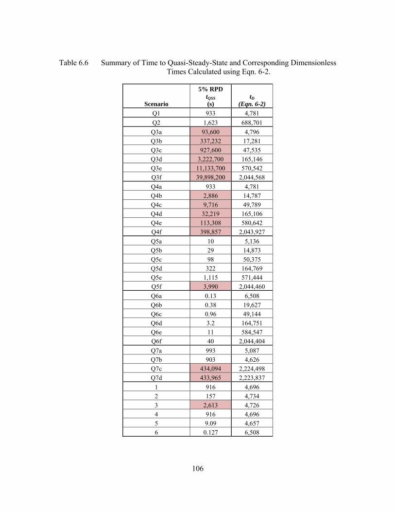
106
Table 6.6 Summary of Time to Quasi-Steady-State and Corresponding Dimensionless Times Calculated using Eqn. 6-2.
Scenario
5% RPD tQSS (s)
tD (Eqn. 6-2)
Q1 933 4,781 Q2 1,623 688,701 Q3a 93,600 4,796 Q3b 337,232 17,281 Q3c 927,600 47,535 Q3d 3,222,700 165,146 Q3e 11,133,700 570,542 Q3f 39,898,200 2,044,568 Q4a 933 4,781 Q4b 2,886 14,787 Q4c 9,716 49,789 Q4d 32,219 165,106 Q4e 113,308 580,642 Q4f 398,857 2,043,927 Q5a 10 5,136 Q5b 29 14,873 Q5c 98 50,375 Q5d 322 164,769 Q5e 1,115 571,444 Q5f 3,990 2,044,460 Q6a 0.13 6,508 Q6b 0.38 19,627 Q6c 0.96 49,144 Q6d 3.2 164,751 Q6e 11 584,547 Q6f 40 2,044,404 Q7a 993 5,087 Q7b 903 4,626 Q7c 434,094 2,224,498 Q7d 433,965 2,223,837
1 916 4,696 2 157 4,734 3 2,613 4,726 4 916 4,696 5 9.09 4,657 6 0.127 6,508
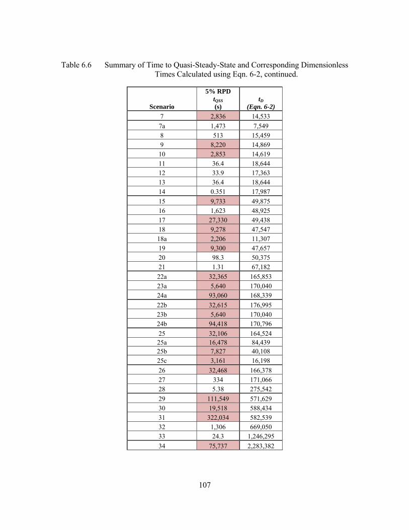
107
Table 6.6 Summary of Time to Quasi-Steady-State and Corresponding Dimensionless Times Calculated using Eqn. 6-2, continued.
Scenario
5% RPD tQSS (s)
tD (Eqn. 6-2)
7 2,836 14,533 7a 1,473 7,549 8 513 15,459 9 8,220 14,869
10 2,853 14,619 11 36.4 18,644 12 33.9 17,363 13 36.4 18,644 14 0.351 17,987 15 9,733 49,875 16 1,623 48,925 17 27,330 49,438 18 9,278 47,547 18a 2,206 11,307 19 9,300 47,657 20 98.3 50,375 21 1.31 67,182 22a 32,365 165,853 23a 5,640 170,040 24a 93,060 168,339 22b 32,615 176,995 23b 5,640 170,040 24b 94,418 170,796 25 32,106 164,524 25a 16,478 84,439 25b 7,827 40,108 25c 3,161 16,198 26 32,468 166,378 27 334 171,066 28 5.38 275,542 29 111,549 571,629 30 19,518 588,434 31 322,034 582,539 32 1,306 669,050 33 24.3 1,246,295 34 75,737 2,283,382
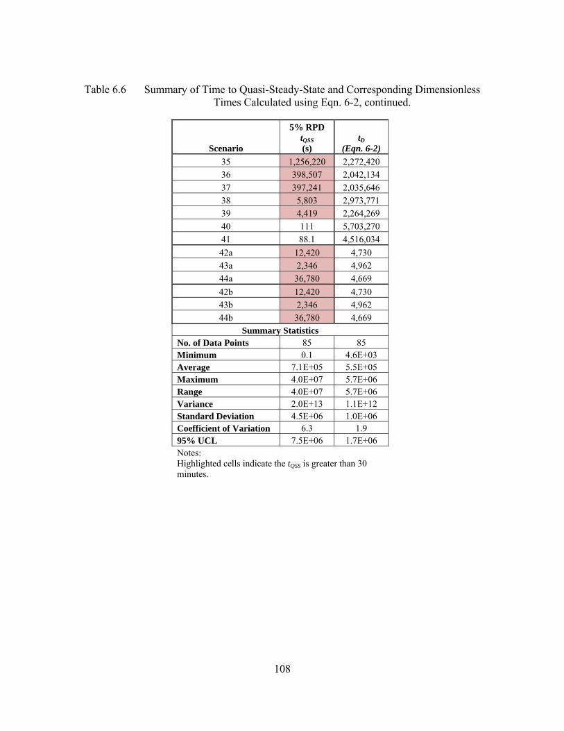
108
Table 6.6 Summary of Time to Quasi-Steady-State and Corresponding Dimensionless Times Calculated using Eqn. 6-2, continued.
Scenario
5% RPD tQSS (s)
tD (Eqn. 6-2)
35 1,256,220 2,272,420 36 398,507 2,042,134 37 397,241 2,035,646 38 5,803 2,973,771 39 4,419 2,264,269 40 111 5,703,270 41 88.1 4,516,034 42a 12,420 4,730 43a 2,346 4,962 44a 36,780 4,669 42b 12,420 4,730 43b 2,346 4,962 44b 36,780 4,669
Summary StatisticsNo. of Data Points 85 85 Minimum 0.1 4.6E+03 Average 7.1E+05 5.5E+05 Maximum 4.0E+07 5.7E+06 Range 4.0E+07 5.7E+06 Variance 2.0E+13 1.1E+12 Standard Deviation 4.5E+06 1.0E+06 Coefficient of Variation 6.3 1.9 95% UCL 7.5E+06 1.7E+06 Notes: Highlighted cells indicate the tQSS is greater than 30 minutes.

109
Figure 6.2 Relationship between tD as defined by Eqn. 6-2 and time to quasi-steady-state.
The visual representation of the relationship between tD and time to quasi-steady-
state provided in Figure 6.2 indicates that the aquifer thickness, b, is an important factor
in the time to quasi-steady-state (as evidenced by the clustering of results).
Careful examination of the results shown in Table 6.6 indicates a correlation
between the overall aquifer thickness (b) and time to quasi-steady-state as well as
between hydraulic conductivity (K) and time to quasi-steady-state, and possibly between
hydraulic diffusivity (D) and time to quasi-steady-state. Based on this observation, three
new non-dimensionalizations for time were considered:
∑
∑
=
== n
iiSi
n
iii
D
bS
bK
btt
1
12
(6-3)
1.E-02
1.E+00
1.E+02
1.E+04
1.E+06
1.E-01 1.E+01 1.E+03 1.E+05 1.E+07
t D(E
qn. 6
-2)
Time to Quasi-Steady-State (s)

110
∑
∑
=
== n
i i
i
n
i Si
i
D
KbSb
btt
1
12
(6-4)
min2 DbttD = (6-5)
The first of these non-dimensionalizations (Eqn. 6-3), is similar to Eqn. 6-2, with
b substituted for r, since it appears from observation of the results in Table 6.1 and Figure
6.2 that the time to quasi-steady-state is at least partially a function of b. The second
non-dimensionalization (Eqn. 6-4) is based on a harmonic average of the hydraulic
conductivities (K) for a given system; the harmonic average is often used to determine
equivalent K values for systems where flow is perpendicular to the system layers (e.g. as
with crossflow). The last non-dimensionalization (Eqn. 6-5) employs the minimum
hydraulic diffusivity (Dmin). The results of these non-dimensionalizations are included in
Table 6.7. The summary statistics for the non-dimensionalizations are also included in
Table 6.7.
The non-dimensionalization employing Dmin (Eqn. 6-5) exhibits the smallest range
of results (0.20 to 0.66), the smallest variance across the dataset (0.013), the smallest
standard deviation (0.12), and the smallest coefficient of variation (0.47), indicating that
of the non-dimensionalizations employed, this is the best mathematically for the purposes
of predicting time to quasi-steady-state. Looking at the dataset as a whole for the Dmin
non-dimensionalization (Eqn. 6-5), the average tD is 0.25. The 95% upper confidence
111
limit (UCL)1 for this dataset is tD=0.30. In theory, this value for tD defined by Eqn. 6-5
should reasonably serve as a predictive tool (in the absence of site-specific information)
for the time to quasi-steady-state (defined by the time where the hydraulic gradients are
approximately 5% RPD) in 95% of cases.
1 The UCL values were determined using the United States Environmental Protection Agency (USEPA) software ProUCL 4.0 (USEPA, 2008).
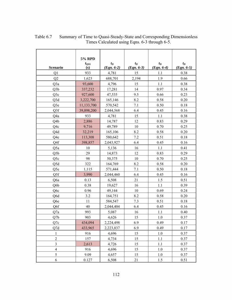
112
Table 6.7 Summary of Time to Quasi-Steady-State and Corresponding Dimensionless Times Calculated using Eqns. 6-3 through 6-5.
Scenario
5% RPD tQSS (s)
tD (Eqn. 6-2)
tD (Eqn. 6-3)
tD (Eqn. 6-4)
tD (Eqn. 6-5)
Q1 933 4,781 15 1.1 0.38 Q2 1,623 688,701 2,194 1.9 0.66 Q3a 93,600 4,796 15 1.1 0.38 Q3b 337,232 17,281 14 0.97 0.34 Q3c 927,600 47,535 9.5 0.66 0.23 Q3d 3,222,700 165,146 8.2 0.58 0.20 Q3e 11,133,700 570,542 7.1 0.50 0.18 Q3f 39,898,200 2,044,568 6.4 0.45 0.16 Q4a 933 4,781 15 1.1 0.38 Q4b 2,886 14,787 12 0.83 0.29 Q4c 9,716 49,789 10 0.70 0.25 Q4d 32,219 165,106 8.2 0.58 0.20 Q4e 113,308 580,642 7.2 0.51 0.18 Q4f 398,857 2,043,927 6.4 0.45 0.16 Q5a 10 5,136 16 1.1 0.41 Q5b 29 14,873 12 0.83 0.29 Q5c 98 50,375 10 0.70 0.25 Q5d 322 164,769 8.2 0.58 0.20 Q5e 1,115 571,444 7.1 0.50 0.18 Q5f 3,990 2,044,460 6.4 0.45 0.16 Q6a 0.13 6,508 21 1.5 0.51 Q6b 0.38 19,627 16 1.1 0.39 Q6c 0.96 49,144 10 0.69 0.24 Q6d 3.2 164,751 8.2 0.58 0.20 Q6e 11 584,547 7.3 0.51 0.18 Q6f 40 2,044,404 6.4 0.45 0.16 Q7a 993 5,087 16 1.1 0.40 Q7b 903 4,626 15 1.0 0.37 Q7c 434,094 2,224,498 6.9 0.49 0.17 Q7d 433,965 2,223,837 6.9 0.49 0.17
1 916 4,696 15 1.0 0.37 2 157 4,734 15 1.1 0.37 3 2,613 4,726 15 1.1 0.37 4 916 4,696 15 1.0 0.37 5 9.09 4,657 15 1.0 0.37 6 0.127 6,508 21 1.5 0.51
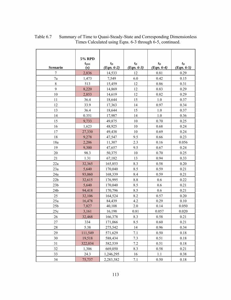
113
Table 6.7 Summary of Time to Quasi-Steady-State and Corresponding Dimensionless Times Calculated using Eqns. 6-3 through 6-5, continued.
Scenario
5% RPD tQSS (s)
tD (Eqn. 6-2)
tD (Eqn. 6-3)
tD (Eqn. 6-4)
tD (Eqn. 6-5)
7 2,836 14,533 12 0.81 0.29 7a 1,473 7,549 6.0 0.42 0.15 8 513 15,459 12 0.86 0.31 9 8,220 14,869 12 0.83 0.29
10 2,853 14,619 12 0.82 0.29 11 36.4 18,644 15 1.0 0.37 12 33.9 17,363 14 0.97 0.34 13 36.4 18,644 15 1.0 0.37 14 0.351 17,987 14 1.0 0.36 15 9,733 49,875 10 0.70 0.25 16 1,623 48,925 10 0.68 0.24 17 27,330 49,438 10 0.69 0.24 18 9,278 47,547 9.5 0.66 0.23 18a 2,206 11,307 2.3 0.16 0.056 19 9,300 47,657 9.5 0.67 0.24 20 98.3 50,375 10 0.70 0.25 21 1.31 67,182 13 0.94 0.33 22a 32,365 165,853 8.3 0.58 0.20 23a 5,640 170,040 8.5 0.59 0.21 24a 93,060 168,339 8.4 0.59 0.21 22b 32,615 176,995 8.8 0.6 0.22 23b 5,640 170,040 8.5 0.6 0.21 24b 94,418 170,796 8.5 0.6 0.21 25 32,106 164,524 8.2 0.57 0.20 25a 16,478 84,439 4.2 0.29 0.10 25b 7,827 40,108 2.0 0.14 0.050 25c 3,161 16,198 0.81 0.057 0.020 26 32,468 166,378 8.3 0.58 0.21 27 334 171,066 8.5 0.60 0.21 28 5.38 275,542 14 0.96 0.34 29 111,549 571,629 7.1 0.50 0.18 30 19,518 588,434 7.3 0.51 0.18 31 322,034 582,539 7.2 0.51 0.18 32 1,306 669,050 8.3 0.58 0.21 33 24.3 1,246,295 16 1.1 0.38 34 75,737 2,283,382 7.1 0.50 0.18
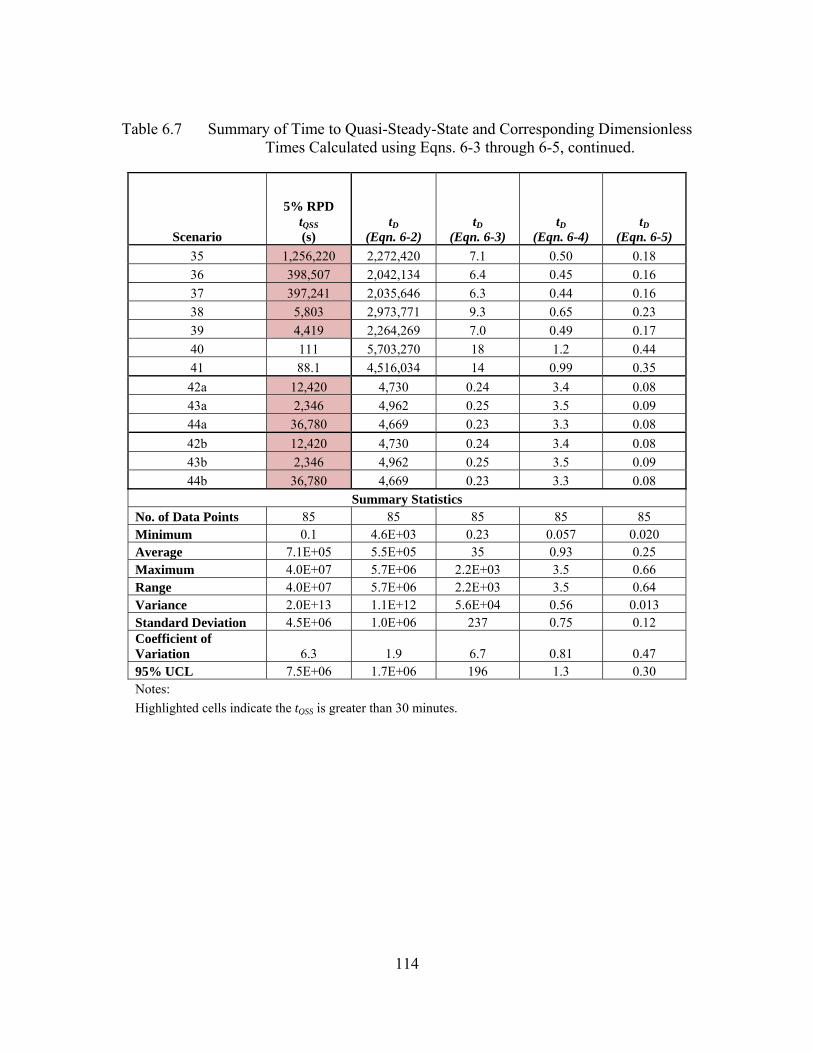
114
Table 6.7 Summary of Time to Quasi-Steady-State and Corresponding Dimensionless Times Calculated using Eqns. 6-3 through 6-5, continued.
Scenario
5% RPD tQSS (s)
tD (Eqn. 6-2)
tD (Eqn. 6-3)
tD (Eqn. 6-4)
tD (Eqn. 6-5)
35 1,256,220 2,272,420 7.1 0.50 0.18 36 398,507 2,042,134 6.4 0.45 0.16 37 397,241 2,035,646 6.3 0.44 0.16 38 5,803 2,973,771 9.3 0.65 0.23 39 4,419 2,264,269 7.0 0.49 0.17 40 111 5,703,270 18 1.2 0.44 41 88.1 4,516,034 14 0.99 0.35 42a 12,420 4,730 0.24 3.4 0.08 43a 2,346 4,962 0.25 3.5 0.09 44a 36,780 4,669 0.23 3.3 0.08 42b 12,420 4,730 0.24 3.4 0.08 43b 2,346 4,962 0.25 3.5 0.09 44b 36,780 4,669 0.23 3.3 0.08
Summary StatisticsNo. of Data Points 85 85 85 85 85 Minimum 0.1 4.6E+03 0.23 0.057 0.020 Average 7.1E+05 5.5E+05 35 0.93 0.25 Maximum 4.0E+07 5.7E+06 2.2E+03 3.5 0.66 Range 4.0E+07 5.7E+06 2.2E+03 3.5 0.64 Variance 2.0E+13 1.1E+12 5.6E+04 0.56 0.013 Standard Deviation 4.5E+06 1.0E+06 237 0.75 0.12 Coefficient of Variation 6.3 1.9 6.7 0.81 0.47 95% UCL 7.5E+06 1.7E+06 196 1.3 0.30 Notes: Highlighted cells indicate the tQSS is greater than 30 minutes.
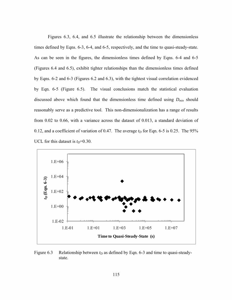
115
Figures 6.3, 6.4, and 6.5 illustrate the relationship between the dimensionless
times defined by Eqns. 6-3, 6-4, and 6-5, respectively, and the time to quasi-steady-state.
As can be seen in the figures, the dimensionless times defined by Eqns. 6-4 and 6-5
(Figures 6.4 and 6.5), exhibit tighter relationships than the dimensionless times defined
by Eqns. 6-2 and 6-3 (Figures 6.2 and 6.3), with the tightest visual correlation evidenced
by Eqn. 6-5 (Figure 6.5). The visual conclusions match the statistical evaluation
discussed above which found that the dimensionless time defined using Dmin should
reasonably serve as a predictive tool. This non-dimensionalization has a range of results
from 0.02 to 0.66, with a variance across the dataset of 0.013, a standard deviation of
0.12, and a coefficient of variation of 0.47. The average tD for Eqn. 6-5 is 0.25. The 95%
UCL for this dataset is tD=0.30.
Figure 6.3 Relationship between tD as defined by Eqn. 6-3 and time to quasi-steady-state.
1.E-02
1.E+00
1.E+02
1.E+04
1.E+06
1.E-01 1.E+01 1.E+03 1.E+05 1.E+07
t D(E
qn. 6
-3)
Time to Quasi-Steady-State (s)
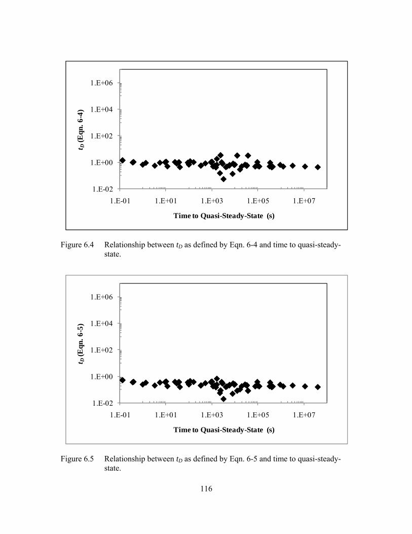
116
Figure 6.4 Relationship between tD as defined by Eqn. 6-4 and time to quasi-steady-state.
Figure 6.5 Relationship between tD as defined by Eqn. 6-5 and time to quasi-steady-state.
1.E-02
1.E+00
1.E+02
1.E+04
1.E+06
1.E-01 1.E+01 1.E+03 1.E+05 1.E+07
t D(E
qn. 6
-4)
Time to Quasi-Steady-State (s)
1.E-02
1.E+00
1.E+02
1.E+04
1.E+06
1.E-01 1.E+01 1.E+03 1.E+05 1.E+07
t D(E
qn. 6
-5)
Time to Quasi-Steady-State (s)
117
Now that a non-dimensionalization has been selected for time to quasi-steady-
state defined by the time where the hydraulic gradients are approximately 5% RPD, this
non-dimensionalization may be applied to the subjective time to quasi-steady-state (Table
6.8). The 95% UCL for this non-dimensionalized dataset is 0.11. As with the times at
5% RPD, this value should reasonably serve as a predictive tool for the subjective time to
quasi-steady-state in 95% of cases. It is important to note; however, that because this is a
UCL, this value may overshoot the actual pumping duration required to attain meaningful
flowmeter readings.

118
Table 6.8 Summary of Subjective Time to Quasi-Steady-State and Corresponding Dimensionless Times Calculated using Eqn. 6-5.
Scenario
Subjective tQSS (s)
tD (Eqn. 6-5)
Q1 18 0.0074 Q2 8.2 0.0033 Q3a NA NA Q3b NA NA Q3c NA NA Q3d NA NA Q3e NA NA Q3f NA NA Q4a 18 0.0074 Q4b 246 0.025 Q4c 1,049 0.027 Q4d 1,180 0.0075 Q4e 3,600 0.0057 Q4f 262 0.00010 Q5a 6.0 0.24 Q5b NA NA Q5c NA NA Q5d NA NA Q5e NA NA Q5f NA NA Q6a NA NA Q6b NA NA Q6c NA NA Q6d NA NA Q6e NA NA Q6f NA NA Q7a 63 0.025 Q7b 33 0.013 Q7c 262 0.00010 Q7d 262 0.00010
1 16 0.0066 2 6.0 0.014 3 123 0.018 4 31 0.013 5 0.54 0.022 6 0.015 0.061

119
Table 6.8 Summary of Subjective Time to Quasi-Steady-State and Corresponding Dimensionless Times Calculated using Eqn. 6-5, continued.
Scenario
Subjective tQSS (s)
tD (Eqn. 6-5)
7 63 0.0064 7a 13 0.0013 8 63 0.037 9 273 0.0097
10 153 0.015 11 2.0 0.021 12 2.0 0.021 13 2.0 0.021 14 0.13 0.13 15 1,049 0.027 16 63 0.0093 17 1,049 0.0094 18 262 0.0066 18a 8.2 0.0002 19 186 0.0047 20 8.2 0.021 21 0.61 0.15 22a 66 0.00041 23a 16 0.001 24a 246 0.0005 22b 213 0.0014266 23b 33 0.0012193 24b 328 0.0007316 25 33 0.00021 25a 33 0.00021 25b 4.1 0.00003 25c 16 0.00010 26 33 0.00021 27 10 0.0065 28 3.19 0.20 29 3,600 0.0057 30 524 0.0049 31 5,216 0.0029 32 241 0.038 33 18 0.29 34 524 0.0012
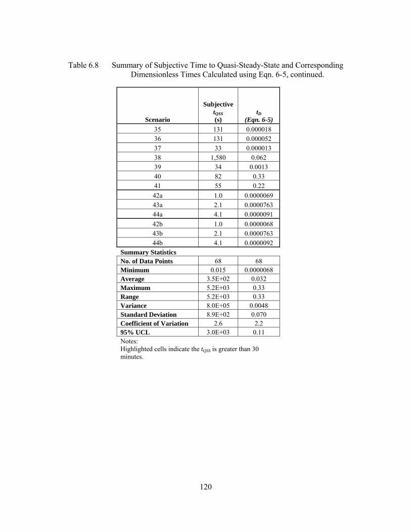
120
Table 6.8 Summary of Subjective Time to Quasi-Steady-State and Corresponding Dimensionless Times Calculated using Eqn. 6-5, continued.
Scenario
Subjective tQSS (s)
tD (Eqn. 6-5)
35 131 0.000018 36 131 0.000052 37 33 0.000013 38 1,580 0.062 39 34 0.0013 40 82 0.33 41 55 0.22 42a 1.0 0.0000069 43a 2.1 0.0000763 44a 4.1 0.0000091 42b 1.0 0.0000068 43b 2.1 0.0000763 44b 4.1 0.0000092
Summary Statistics No. of Data Points 68 68 Minimum 0.015 0.0000068 Average 3.5E+02 0.032 Maximum 5.2E+03 0.33 Range 5.2E+03 0.33 Variance 8.0E+05 0.0048 Standard Deviation 8.9E+02 0.070 Coefficient of Variation 2.6 2.2 95% UCL 3.0E+03 0.11 Notes: Highlighted cells indicate the tQSS is greater than 30 minutes.
121
CHAPTER 7
CONCLUSIONS
Resolution of Literature Findings
Through a comparison of the published models [Katz and Tek 1962; Javandel and
Witherspoon 1969; Ruud and Kabala 1996; Hemker 1999a, 1999b; Kabala and El-
Sayegh 2002] and the use of an independent model capable of accurately and reliably
reproducing the primary results of the published models while addressing the smaller
inconsistencies between them, meaningful and conclusive data regarding the hydraulic
gradient behavior for layered systems was obtained. Single-domain, multi-layer confined
aquifers with homogeneous and isotropic or anisotropic layers were evaluated for a
variety of aquifer parameters during this study.
To better understand the factors influencing hydraulic gradient behavior in multi-
layer, confined aquifers, the numerical model TMVOC was employed in this study. This
model makes no simplifying assumptions other than boundary condition assumptions and
successfully reproduced or resolved the primary results published by other researchers on
related topics. Whereas none of the four published studies discussed throughout this
report [Katz and Tek 1962; Javandel and Witherspoon 1969; Ruud and Kabala 1996,
1997; Hemker 1999a, 199b; Kabala and El-Sayegh 2002] focused solely on hydraulic
gradient behavior, qualitative statements were made regarding the effects of aquifer
properties on crossflow and other factors influencing the time required for a system to
reach quasi-steady-state.

122
The difference between the Ruud and Kabala [1997] and Javandel and
Witherspoon [1969] conclusions is the most significant theoretical difference between the
models examined in this study. The other differences in conclusions between the
published models involve small-scale boundary effects (Ruud and Kabala [1996, 1997]
and Hemker [1999a, 1999b]) and increases in error with increases in hydraulic diffusivity
[Kabala and El-Sayegh 2002]. Based on the comparison of the models and the results
obtained here, it is likely, given the small magnitude of these differences, that differences
in the approximation of the layer interfaces and grid formation are responsible. The
primary difference in implementation between the four published models is the solution
of the system at the layer interface. The differences in grid formulation can be
disregarded as insignificant compared to the solution at the layer interface, as each of the
models was analyzed for errors and a sufficiently dense grid was used to satisfy error
criteria.
The solution of the crossflow components has been handled implicitly [Javandel
and Witherspoon 1969], approximately using increases in grid density and employing
averages in K [Ruud and Kabala 1996, 1997; Hemker 1999a, 1999b], and by assuming
crossflow to be in pseudo-steady-state [Kabala and El-Sayegh 2000]. Only by using the
continuity equation at the layer interface or by implicitly solving the system using an
integral finite difference grid, can the crossflow component be solved exactly. These
approaches in-turn minimize the overall numerical error of the model by solving the term
directly. The scenarios assessed during this study were each modeled using TMVOC, an
integral finite difference model.
123
Ruud and Kabala [1996] and Javandel and Witherspoon [1969]
The results of Ruud and Kabala’s modeling efforts suggest that, contrary to the
Theis [1935] model and the results of Javandel and Witherspoon [1969] model, the flux
along the wellbore for some layers may be persistently transient or non-uniform. The
Theis [1935] model assumes that flows toward a well in layered aquifers are uniform and
quickly become horizontal, which is what the Javandel and Witherspoon [1969] model
confirms. The Ruud and Kabala [1996] model findings therefore deviate from the
Javandel and Witherspoon [1969] model findings and are inconsistent with the Theis
[1935] solution. Based on these findings, Ruud and Kabala [1996] conclude that the
Theis [1935] model may be inadequate and too simplistic in nature to accurately describe
the hydraulic behavior of layered aquifers. Another key finding of the Ruud and Kabala
[1996] study was the confirmation of the Kabala [1994] results indicating that the
hydraulic diffusivity contrast between adjacent layers, rather than the magnitude of the
corresponding K ratio, is the dominant factor for accurately estimating parameters in the
flowmeter analyses.
The seemingly conflicting statements of the time required for quasi-steady-state
from Javandel and Witherspoon [1969] (i.e., short times to quasi-steady-state) and Ruud
and Kabala [1997] (i.e., persistently transient conditions for some situation) have been
resolved here. This study has found results analogous to those of Ruud and Kabala
[1996] in that the layer flows in many systems in this study required longer than the
dimensionless time of 1,000 defined by Javandel and Witherspoon [1996] for individual
layer flows to equilibrate. As was demonstrated in the Section 6, the use of this particular
124
dimensionless time for the prediction of quasi-steady-state is not appropriate and a non-
dimensional time based on the aquifer Dmin was defined.
Additionally, data included in Figure 5 from Ruud and Kabala [1996] was
analyzed using the flowmeter methodology and equations. The finding of this analysis
was that, for the purposes of most applications, the real-world difference between the
calculated-K and input-K values was not significant. Furthermore, the calculated-K for
the dominant layer in the system (i.e., the high-K layer, with respect to transport or
productivity) is consistent with the input value for even the earliest time included in the
figure.
Ruud and Kabala’s [1996] assertion that the Theis solution was overly simplistic
was based in part on their findings that the layer flows into the well are persistently
transient. It has been demonstrated that while this is true mathematically, the transient
nature of the flows is not an issue except at very early times. This is based on the finding
of this study that representative K values may be obtained from the flowmeter test as
early in the pumping as when the hydraulic head gradients are within 64% RPD on
average.
Application of Findings to EBF Testing
The ability of the flowmeter test and data analysis to rapidly resolve high-K layers
is an important feature of the analysis. As has been shown throughout this study, the
hydraulic gradients at the well associated with high-K layers resolve rapidly to their
steady-state values, with the lower-K layers requiring more time and in many cases, the
lowest-K layer may not resolve during a flowmeter test. More importantly, the flowmeter
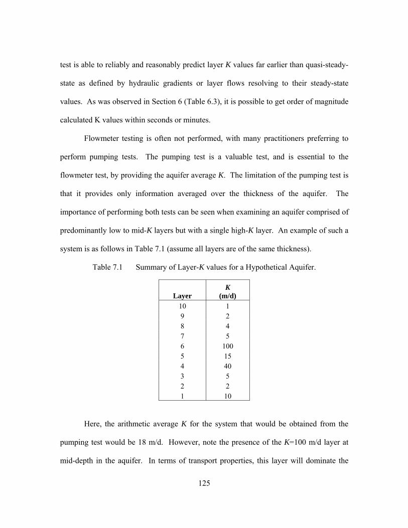
125
test is able to reliably and reasonably predict layer K values far earlier than quasi-steady-
state as defined by hydraulic gradients or layer flows resolving to their steady-state
values. As was observed in Section 6 (Table 6.3), it is possible to get order of magnitude
calculated K values within seconds or minutes.
Flowmeter testing is often not performed, with many practitioners preferring to
perform pumping tests. The pumping test is a valuable test, and is essential to the
flowmeter test, by providing the aquifer average K. The limitation of the pumping test is
that it provides only information averaged over the thickness of the aquifer. The
importance of performing both tests can be seen when examining an aquifer comprised of
predominantly low to mid-K layers but with a single high-K layer. An example of such a
system is as follows in Table 7.1 (assume all layers are of the same thickness).
Table 7.1 Summary of Layer-K values for a Hypothetical Aquifer.
Layer K
(m/d) 10 1 9 2 8 4 7 5 6 100 5 15 4 40 3 5 2 2 1 10
Here, the arithmetic average K for the system that would be obtained from the
pumping test would be 18 m/d. However, note the presence of the K=100 m/d layer at
mid-depth in the aquifer. In terms of transport properties, this layer will dominate the
126
system behavior, but is not reflected properly in the pumping test. In fact, the pumping
test could underestimate transport velocities by more than a factor of 5. Now, imagine
that this highest-K layer is thinner than the lower-K layers. The transport velocity
potential of the highest-K layer would be the same, but the average K obtained from the
pumping test would be biased even lower than the 18 m/d obtained for the all layers of
equal thickness scenario. This simple example illustrates the importance of performing
flowmeter tests in addition to pumping tests.
Summary of Findings
To summarize, the various influences of system parameters on hydraulic gradient
behavior in multi-layer confined aquifers in response to a pumping influence are:
1. Aquifer Thickness: The time to attain quasi-steady-state is a function of
the ratio of the hydraulic diffusivities (D) between the layers as well as the
overall aquifer thickness (b). As b is increased, the time to quasi-steady-
state increases according to a power relationship. The relationship is a
power relationship, indicating that the increase in the time required to
attain quasi-steady-state is small at smaller thicknesses and becomes larger
between successive increases in aquifer thickness. However, the results of
the scenarios modeled during this study show that representative K values
may be obtained far earlier (at 64% RPD) than the quasi-steady-state
defined by the time when the hydraulic gradients are within 5% RPD of
each other.
127
2. Layer Thickness: As the layer thickness is decreased, the time to quasi-
steady-state decreases in a linear fashion. However the times remain
greater than that for the minimum scenario (Scenario Q1, b=0.9 m) even
when the layers are the same thickness and arrangement as employed in
Scenario Q1. This reinforces the conclusions from the aquifer thickness
analysis that as the overall aquifer thickness is increased, the time to
quasi-steady-state increases.
3. Pumping Rate: In general, increasing the QP resulted in small differences
in the time required to attain quasi-steady-state. Therefore, pumping rate
is not considered to be a significant factor in the time needed to attain
quasi-steady-state, and the pumping rate should be selected based on the
study limitations (i.e., time, purge water disposal costs/options, etc.).
4. Layer Arrangement: The arrangement of layers in a system, all other
parameters being equal, does not significantly affect the time to subjective
quasi-steady-state for the thin systems analyzed. However, the thick
systems did experience differences in times to quasi-steady-state, where
the scenarios with largest times to quasi-steady-state are those where the
lower-K layers are adjacent to one another with the lowest-K layer located
adjacent to a boundary condition (Scenarios Q7a and Q7c). In both
thicknesses, the subjective times to quasi-steady-state were identical for
the three layer arrangements, however, indicating that the layer
arrangement will not influence the flowmeter results.

128
5. Hydraulic Diffusivity, Part 1: The time to quasi-steady-state as a function
of Ss is linear. All other parameters being equal, systems with larger Ss
take longer to reach quasi-steady-state than those with smaller Ss. This is
due to an increase in available water volume for release from storage and
the longer time period over which this release occurs.
6. Hydraulic Diffusivity, Part 2: Systems where D is constant over the
thickness of the system results in nearly instantaneous times to quasi-
steady-state. These results confirm in part the findings from Ruud and
Kabala [1994, 1996] that the ratio of D between layers (rather than the K
ratio between layers) is important in determining the transient behavior of
the hydraulic head gradients.
7. Hydraulic Diffusivity, Part 3: The times to quasi-steady-state for systems
with homogeneous K and variable Ss are, on average, half that of the non-
homogeneous K and constant Ss systems. Two conclusions may be draw
from these results:
a. Holding K uniform throughout the system results in no crossflow
between the three layers due to hydraulic head differences
resulting from K; the hydraulic head differences in these situations
must therefore be a function of a system’s D distribution. Again,
this supports in part the findings from Ruud and Kabala [1996].
b. The case of a homogeneous K appears to be a special case. Based
on this finding, it is not possible to say that D is the sole driving
129
force behind the time required to attain quasi-steady-state. Were
that the case, systems of the same configuration and with the same
D distribution should attain quasi-steady-state at the same time.
The results from this study show this to not be the case; rather,
both the Ss and K-distributions play a role. Crossflow influences
related to hydraulic head differences as a function of Ss play a
smaller role in the transient behavior of the hydraulic head
gradients than differences in K.
8. Hydraulic Diffusivity, Part 4: The sum of these conclusions is that
although D is important, it is not the sole parameter determining the
behavior of hydraulic gradients under pumping conditions. Aquifer
thickness and layer thickness also both play an important role in the
gradient behavior.
9. Anisotropy: As the vertical K of the layers is increased, the amount of
crossflow at early times increases, resulting in a smaller time to quasi-
steady-state. This behavior confirms the findings of Katz and Tek [1962]
who found that the upper limit for crossflow occurs when the vertical
hydraulic conductivity (Kz) approaches infinity compared to the horizontal
hydraulic conductivity (Kr). In other words, as the vertical hydraulic
conductivity (Kz) increases relative to the horizontal hydraulic
conductivity (Kr), resistance to crossflow decreases and the time over
130
which crossflow significantly affects the overall system behavior
decreases.
10. RPD: The initial hypothesis that systems should be considered to be in
quasi-steady-state when the maximum difference between hydraulic
gradients at the well were approximately 5% is found to be too stringent.
Given the large times to quasi-steady-state reflected by the 5% RPD
criteria, the data were evaluated to determine at what time did the
flowmeter analysis yield calculated K values representative of the input
values. These subjective times to quasi-steady-state yielded representative
K values as early in the pumping as when the hydraulic head gradients are
within 64% RPD on average and in many cases at larger RPDs. This is an
important finding because it demonstrates that it is possible to obtain
representative K values for an aquifer during the period when flow into the
well (which is directly proportional to the gradient at the well) is still
transient.
11. The non-dimensionalization of time developed by Javandel and
Witherspoon [1969] and employed by Ruud and Kabala [1996] was found
to be a poor tool for predicting time to quasi-steady-state. Rather, a
relationship incorporating Dmin and the aquifer thickness was found to be a
good predictor of subjective time to quasi-steady-state (Eqn 6-5):
min2 DbttD = (7-1)
131
The 95% UCL for the non-dimensionalization of the subjective time to
quasi-steady-state was determined to be tD=0.11. This value should
reasonably serve as a predictive tool for the subjective time to quasi-
steady-state in 95% of cases.
132
REFERENCES
Anderson, M. P. and Woessner, W. W. 1992. Applied Groundwater Modeling. Academic Press, San Diego, California.
Arnold, K. B. and Molz, F. J. 2000. In-well hydraulics of the electromagnetic borehole flowmeter: further studies. Ground Water Monitoring & Remediation. Winter:52-55.
Batu, V. 1998. Aquifer Hydraulics A Comprehensive Guide to Hydrogeologic Data Analysis. John Wiley & Sons, Hoboken, New Jersey.
Boggs, J. M.; Young, S. C.; Beard, L. M.; Gelhar, L. W.; Rehfeldt, K. R.; and Adams, E. E. 1990. Field study of dispersion in a heterogeneous aquifer 1: Overview and site description. Water Resources Research. 28:3281-3291.
Boman, G. K.; Molz, F. J.; and Boone, K. D. 1997. Borehole flowmeter application in fluvial sediments: methodology, results, and assessment. Ground Water. 35(3):443-450.
Cooley, R. L. 1971. A finite difference method for unsteady flow in a variably saturated porous media: application to a single pumping well. Water Resources Research. 7(6): 1607-1625.
Cooper, Jr., H. H. and Jacob, C. E. 1946. A generalized graphical method for evaluations of formation constants and summarizing well-field history. Transactions of the American Geophysical Union. 27:526-534.
Crisman, S. A.; Molz, F. J.; Dunn, D. L.; and Sappington, F. C. 2001. Application for the Electromagnetic Borehole Flowmeter in Shallow Unconfined Aquifers. Groundwater Monitoring & Remediation. Fall:96-100.
De Hoog, F. R., Knight, J. H., and Stokes, A. N. 1982. An improved method for numerical inversion of Laplace transforms. SIAM Journal on Scientific and Statistical Computing. 3:357-366.
Dinwiddie, C. L.; Foley, N. A.; and Molz, F. J. 1999. In-well hydraulics of the electromagnetic borehole flowmeter. Ground Water. 37(2):305-315.
Elci, A., Molz, F.J., and Waldrop, W. R. 2001. Implications of Observed and Simulated Ambient Flow in Monitoring Wells. Ground Water, v. 36, no. 6, pp. 853-862.
133
Finsterle, S.; Kowalsky, M.; Rutqvist, J.; and Xu, T. 2006. IAEA Technical Co-operation Project C7-INT 9.173.009 Numerical Simulation of Subsurface Processes; TOUGH Training Course. August 14-17, 2006. Report No. LBNL-60134. Lawrence Berkely Laboratory. Berkeley, California.
Flach, G. P., Sappington, F. C., Johnson, W. P., and Hiergesell, R. A. 2000. Electromagnetic Borehole Flowmeter (EBF) Testing in R-area (U). Westinghouse Savannah River Company, Report WSRC-2000-00170.
Hantush, M. S. 1964. Hydraulics of Wells. Advances in Hydroscience. Academic Press, New York, pp. 281-442.
Hemker, C. J. 1985. Transient well flow in leaky multiple-aquifer systems. Journal of Hydrology. 81:111-126.
Hemker, C. J. 1999a. Transient well flow in vertically heterogeneous aquifers. Journal of Hydrology. 225:1-18.
Hemker, C. J. 1999b. Transient well flow in layered aquifer systems: the uniform well-face drawdown solution. Journal of Hydrology. 225:19-44.
Hemker, C. J. and Maas, C. 1987. Unsteady flow to wells in layered and fissured aquifer systems. Journal of Hydrology. 90:231-249.
Hunt, B. 1985. Flow to a well in a multilayer aquifer. Water Resources Research. 21(11):1637-1641.
Jaquard, P. 1960. Etude mathematique du drainage d'un reservoir heterogene. Rev. Inst. Frr. Petrole Ann. Combust. Liquides. 15(10):1384.
Javandel, I. and Witherspoon, P. A. 1980. A semianalytical solution for partial penetration in two-layer aquifers. Water Resources Research. 16(6):1099-1106.
Javandel, I. and Witherspoon, P. A. 1983. Analytical solution of a partially penetrating well in a two-layer aquifer. Water Resources Research. 19(2):567-578.
Javandel, I. and Witherspoon, P. A. 1969. A method of analyzing transient fluid flow in multilayered aquifers. Water Resources Research. 5:856-869.
Kabala, Z. J. 1994. Measuring distributions of hydraulic conductivity and specific storativity by the double flowmeter test. Water Resources Research. 30(3):685-690.
Kabala, Z. J. and El-Sayegh, H. K. 2002. Transient flowmeter test: semi-analytic crossflow model. Advances in Water Resources. 25:103-121.
134
Katz, M. L. and Tek, M. R. 1962. A theoretical study of pressure distribution and fluid flux in bounded stratified porous systems with crossflow. Society of Petroleum Engineers Journal. 2(1):68-82.
Lee, T. C. 1998. Applied Mathematics in Hydrogeology. CRC Press.
Maas, C. 1987. Groundwater flow to a well in a layered porous medium 2. Nonsteady multiple-aquifer flow. Water Resources Research. 23(8):1683-1688.
Maidment, D.R. 1993. Handbook of Hydrology. McGraw-Hill Professional.
Molz, F. J.; Guven, O.; Melville, J. G.; and Cardone, C. 1989. Hydraulic conductivity measurement at different scales and contaminant transport modeling. Cushman, J. H., ed. Dynamics of fluids in hierarchal porous media. New York: Academic Press; pp. 35-79.
Molz, F. J. and Young, S. C. 1993. Development and application of borehole flowmeters for environmental assessment. The Log Analyst. 3:13-23.
Moridis, G.J., and Pruess, K. 1995. Flow and Transport Simulations UsingT2CG1, A Package of Preconditioned Conjugate Gradient Solvers for the TOUGH2 Family of Codes, LBL Report No. 36235. Lawrence Berkely Laboratory. Berkeley, California.
Neuman, S. P. and Witherspoon, P. A. 1969. Theory of flow in a confined two aquifer system. Water Resources Research. 5(4):803-816.
Pruess, K. and Battistelli, A. 2002. TMVOC, A Numerical Simulator for Three-Phase Non-isothermal Flows of Multicomponent Hydrocarbon Mixtures in Saturated-Unsaturated Heterogeneous Media. Report No. LBNL-49375. Lawrence Berkely Laboratory. Berkeley, California.
Pruess, K., Oldenburg, C. and Moridis, G. 1999. TOUGH2 User’s Guide, Version 2. Report No. LBNL-43134. Lawrence Berkely Laboratory. Berkeley, California.
Pruess, K., Simmons, A., Wu, Y. S. and Moridis, G. 1996. TOUGH2 Software Qualification. Report No. LBNL-38383. Lawrence Berkely Laboratory. Berkeley, California.
Press, W. H.; Teukolsky, S. A.; Vetterling, W. T.; and Flannery, B. P. 1992, Numerical Recipes in Fortran: The Art of Scientific Computing. Cambridge University Press; pp. 346-347.
135
Rehfeldt, K. R.; Hufschmied, P.; Gelhar, L. W.; and Schaefer, M. E. 1989. The borehole flowmeter techniques for measuring hydraulic conductivity variability: Electric Power Research Institute, Interim Report EM-6511, Palo Alto, California.
Russell, D. G. and Prats, M. 1962. Performance of layered reservoirs with crossflow - single-compressible-fluid case. Society of Petroleum Engineers Journal. 2(1):53-67.
Ruud, N. C. and Kabala, Z. J. 1996. Numerical evaluation of flowmeter test interpretation methodologies. Water Resources Research. 32(4):845-852.
Ruud, N. C. and Kabala, Z. J. 1997. Numerical evaluation of the flowmeter test in a layered aquifer with skin zone. Journal of Hydrology. 203:101-108.
Ruud, N. C.; Kabala, Z. J.; and Molz, F. J. 1999. Evaluation of flowmeter-head loss effects in the flowmeter test. Journal of Hydrology. 224:55-63.
Sen, Z. 1989. Radial flow in vertically graded hydraulic conductivity aquifers. Journal of Hydraulic Engineering. 115(12):1667-1682.
Szekely, F. 1995. Estimation of unsteady, three-dimensional drawdown in single, vertically heterogeneous aquifers. Ground Water. 33(4):669-674.
Theis, C. V. 1935. The relation between the lowering of the piezometric surface and the rate and duration of discharge of a well using ground-water storage. EOS Trans. AGU. 16:519-524.
Thiem, G. 1906. Hydrologishe Methoden (in German), J. M. Gebhardt, Leipzig, Germany.
United States Environmental Protection Agency (USEPA) 2008. ProUCL Version 4.0, a Statistical Software, National Exposure Research Lab, EPA, Las Vegas Nevada. ProUCL 4.0 can be freely downloaded from the USEPA website: http://epa.gov/esd/tsc/TSC_form.htm
Waldrop, W. R. 1995. A summary of hydrogeologic studies with the Electromagnetic Borehole Flowmeter. Report QEC T-102, Quantum Engineering Corporation, 112 Tigitsi Lane, Loudon, Tennessee, 37774, 615-458-0506.
Wolfram, S. 1999. The Mathematica Book, 4th Edition. Wolfram Media and Cambridge University Press, Champaign, Illinois.