an evaluation of current mass flux measurement practices ... · mipt and tcw) would be more ... 4.2...

AN EVALUATION AND IMPLEMENTATION

GUIDE FOR CURRENT GROUNDWATER MASS FLUX MEASUREMENT PRACTICES

THESIS

Jack Grierson Wheeldon III, Major, USAF

AFIT/GEM/ENV/08-M23

DEPARTMENT OF THE AIR FORCE AIR UNIVERSITY

AIR FORCE INSTITUTE OF TECHNOLOGY

Wright-Patterson Air Force Base, Ohio

APPROVED FOR PUBLIC RELEASE; DISTRIBUTION UNLIMITED

The views expressed in this thesis are those of the author and do not reflect the official

policy or position of the United States Air Force, Department of Defense, or the United

States Government.

AFIT/GEM/ENV/08-M23

AN EVALUATION AND IMPLEMENTATION GUIDE FOR CURRENT

GROUNDWATER MASS FLUX MEASUREMENT PRACTICES

THESIS

Presented to the Faculty

Department of Systems and Engineering Management

Graduate School of Engineering and Management

Air Force Institute of Technology

Air University

Air Education and Training Command

In Partial Fulfillment of the Requirements for the

Degree of Master of Science in Engineering Management

Jack Grierson Wheeldon III,

Major, United States Air Force

March 2008

APPROVED FOR PUBLIC RELEASE; DISTRIBUTION UNLIMITED.

AFIT/GEM/ENV/08-M23



Jack Grierson Wheeldon III, BS

Major, United States Air Force

Approved:

// Signed // 24 Mar 08

Dr. Mark N. Goltz (Chairman) date


Dr. Alfred E. Thal Jr. date


Major Sonia E. Leach date

AFIT/GEM/ENV/08-M23

Abstract

Contaminant mass flux is an important parameter needed for decision making at sites

with contaminated groundwater. New and potentially better methods for measuring mass flux

are emerging. This study looks at the conventional transect method (TM), and the newer passive

flux meter (PFM), modified integral pump test (MIPT), and tandem circulating well (TCW)

methods. In order to facilitate transfer and application of these innovative technologies, it is

essential that potential technology users have access to credible information that addresses

technology capabilities, limitations, and costs. This study provides such information on each of

the methods by reviewing implementation practices and comparing the costs of applying the

methods at 16 standardized “template” sites. The results of the analysis are consolidated into a

decision tree that can be used to determine which measurement method would be most effective,

from cost and performance standpoints, in meeting management objectives at a given site.

The study found that, in general: (1) the point methods (i.e. the TM and PFM) were less

expensive to use to characterize smaller areas of contamination while the pumping methods (the

MIPT and TCW) would be more economical for larger areas, (2) the pumping methods are not

capable of high resolution sampling, which may be required to characterize heterogeneous

systems or to design remediations, and (3) when high resolution is required, the PFM is more

economical then the TM. Finally, the study demonstrated that, arguably, test results of the newer

methods indicate that their accuracy is as good as, or better than, the accuracy of the TM, the

currently accepted method.

iv

Acknowledgments

I would like to convey my gratitude to my thesis advisor, Dr. Mark N. Goltz, for guiding me through this challenging and rewarding experience. His guidance provided the vectoring for my unwieldy efforts. Without his insight, patience, and instruction this thesis would not be possible. Additionally, I would like to thank Dr. Alfred E. Thal Jr. for his teachings and lightheartedness which provided me with the tools and a voice of reason when under the stresses of graduate school. I would also like to thank Major Sonia Leach for her professional guidance and overall support.

My sincerest thanks to Drs. Michael C. Brooks and A. Lynn Wood of the United States Environmental Protection Agency for their professional assistance in this study.

This study was partially supported by (1) an interagency agreement between the Air Force Institute of Technology (AFIT) and the Ground Water and Ecosystem Restoration Division (GWERD) of the U.S. Environmental Protection Agency National Risk Management Research Laboratory, and (2) Environmental Security Technology Certification Program (ESTCP) Project CU-0318, Diagnostic Tools for Performance Evaluation of Innovative In Situ Remediation Technologies at Chlorinated Solvent-Contaminated Sites. The support of GWERD and ESTCP is gratefully acknowledged.

Most importantly, I am deeply thankful to my family for their unconditional love and support. My wife and children provided me the encouragement and inspiration to persevere when times were tough. I am also extremely grateful to my parents for their support and confidence that have shaped who I am today.

Jack Wheeldon

v

Table of Contents

Page

Abstract……………………………………………………………….………..……..……..…...iv

Acknowledgements………………………………………………….…………………...............v

Table of Contents…………………………………………………………………….…….........vi

List of Figures…………………………………………………………….…………….………...x

List of Tables……………………………………………………………….……………...……xii

I. INTRODUCTION……………………………………………………….……….….…..1

1.1 Motivation………………………………………………………………..….….....…1

1.2 Background……………………………………………………………..…..…....…..4

1.2.1 Transect method (TM)……………..……………….…………….…...…….….5

1.2.2 Passive flux meter (PFM) ………………………………………….…....…….6

1.2.3 Modified integral pump test (MIPT) …………………………………......……7

1.2.4 Tandem Circulating Wells (TCWs) …………………………………..…...…...8

1.3 Research Objectives…………………………………………….…………..…..……9

1.4 Research methodology………………………………..………….………………..…9

1.5 Study Limitations…………………………………………..……………….………10

II. LITERATURE REVIEW…………………….………………………….………….…11 2.1 Introduction………………………………………………………….…..…...……..11

2.2 Mass flux………………………………………………………….……...……….....11

2.3 Flux Measurement Methods …………………………………………..……….….12

2.3.1 Transect method (TM)……………………………………...…………………12

2.3.1.1 Calculating Darcy velocity…………….………………….……....…..14

vi

3.1.1.1 Slug test…………………………………………..…...........14

2.3.1.1.2 Pump test………………………………………….………..15

2.3.1.1.3 Borehole dilution test (BDT)……………………...……….16

2.3.1.2 TM costs…………………………………….……..………………….17

2.3.1.3 TM regulatory concerns……………………….…….…………...…...18

2.3.1.4 TM Advantages and limitations……………………………………....18

2.3.2 Passive flux meters (PFMs)……………………………...…………..……..…20

2.3.2.1 Laboratory and field testing of the PFM…………………….……..…24

2.3.2.2 PFM costs…………………………………………………...………...29

2.3.2.3 Regulatory concerns……………………………………...…………...30

2.3.2.4 PFM Advantages and limitations………………………………...…...30

2.3.3 Tandem circulating wells (TCWs)………………………………………….....31

2.3.3.1 Laboratory testing of the TCW……………………………..………...34

2.3.3.2 TCW Costs…………………………………………………..……..…35

2.3.3.3 TCW regulatory concerns………………………………………….…36

2.3.3.4 TCW Advantages and limitations………………………………....….36

2.3.4 Modified Integral Pump Tests (MIPTs)…………………………………..….37

2.3.4.1 Laboratory and Field Testing of MIPT…………………………….…39

2.3.4.2 MIPT costs…………………………………………………...…….…42

2.3.4.3 MIPT regulatory concerns………………………………..…….….….43

2.3.4.4 MIPT Advantages and limitations…………………………..……..….43

2.4 Method comparison……………………………………………………….…....…..44

vii

5 Cost studies…………………………………………………………..……..……....48

III. METHODOLOGY……………………………………………………...……………...53

3.1 Introduction……………………………………………………...…………….....…53

3.2 Cost Analysis Assumptions………………………………………..…………....….53

3.3 Cost Analysis Methodology…………………………………………….……...…...55

3.3.1 Development of template sites………………………………………..….…...55

3.3.2 Reporting metrics……………………………………………………..….…...56

3.3.3 Application of measurement methods to the template sites…………........…58

3.3.4 Cost for each method………………………………………………..……..…60

3.3.4.1 TM with BDT…………………………………………..….……..….61

3.3.4.2 PFM…………………………………………………….…………....62

3.3.4.3 MIPT………………………………………………………………...64

3.3.4.4 TCW………………………………………………………....……....65

3.4 Decision tree development…………………………..………………..…………....68

IV. RESULTS AND DISCUSSION………………………………….……………..…...…69

4.1 Introduction……………………………………………………………..……….….69

4.2 Published data……………………………………………………...………….....…69

4.2.1 Performance………………………………………………………………...…69

4.2.2 Advantages and limitations………………………………………….……..….70

4.3 Cost comparison……………………………………………………………….....…73

4.3.1 Cost versus size of control plane…………………………………………..…73

viii

3.2 Cost versus required spatial resolution………………………………..….....75

4.3.3 Cost versus hydraulic conductivity…………………………………...…..….78

4.3.4 Cost comparison of all methods…………………………….……………..…80

4.4 Decision tree……………………………………………………………….…...…...87

4.4.1 Notes for decision tree……………………………………..…………………90

4.4.2 Examples for decision tree use………………………………………………93

V. CONCLUSIONS………………………..………………………………………..…..…95

5.1 Summary……………………………………………………………………..……...95 5.2 Conclusions………………………………………………………………………....96 5.3 Recommendations for future research……………………..…………...…...……99

References.………………………………………………………….………………….....100 Appendix A…………………………….…………………………………………………105

ix

List of Figures

Page

Figure 1.1 Groundwater contamination sources (Groundwater Foundation, 2007)………………2

Figure 1.2 Basic configuration of the transect method with multilevel sampling (API, 2003)…...5

Figure 1.3 Flow paths induced by TCW operation………………………………………………..8

Figure 2.1 Cross section showing PFM installation (after Hatfield et al., 2004)…...…...…....…21

Figure 2.2 Fractional flows between TCW screens………...……………………………………33 Figure 2.3 An example of the MIPT approach with multiple pumping wells and one

observation well down gradient…………………………………...…………………39

Figure 4.1 Cost comparisons of methods with varying transect width for 21.3m thick aquifer at low resolution……………………………………………………………..74

Figure 4.2 Point method costs for 21.3m thick aquifer of varying transect length………………76

Figure 4.3 Effect of additional MIPT wells on cost of treating and disposing extracted water…………………………………………….………………………..……….….77

Figure 4.4 Total MIPT cost for measuring contaminant flux for different values of hydraulic

conductivity………………..…………………………………………………………79 Figure 4.5 Influence of hydraulic conductivity on TCW costs…………………………………..80

Figure 4.6 Costs for all measurement methods versus transect width (7.6m thick aquifer)……..81

Figure 4.7 Costs for all measurement methods versus transect width (21.3m thick aquifer)…....81

Figure 4.8 Costs for all measurement methods versus transect width at medium spatial resolution (7.6m thick aquifer)…………………………………...………………….82

Figure 4.9 Costs for all measurement methods versus transect width at medium spatial resolution (21.3m thick aquifer)…………………………………...…………83

Figure 4.10 Costs for all measurement methods versus transect width at high spatial resolution (7.6m thick aquifer)……..………………………….……………………84 Figure 4.11 Costs for all measurement methods versus transect width at high spatial

resolution (21.3m thick aquifer) ..………………………….……………………….84

x

Page

Figure 4.12 Graph of methods applied to 7.6m thick aquifer with different hydraulic conductivities……….…………………………………………………………….…85

Figure 4.13 Graph of methods applied to 21.3 m thick aquifer with different hydraulic

conductivities ……………………………………………………………………….86 Figure 4.14 Decision tree…………………………………………………………………...……89

xi

xii

List of Tables

Page

Table 2.1 Comparison of mass discharge measurement methods at Hill AFB and Ft Lewis (after Brooks et al., 2007)………………………………………..………...................45

Table 2.2 Comparison of methods of measuring Darcy velocity (after USEPA, 2007)…………46

Table 2.3 Comparison of mass flux measurement methods (after USEPA, 2007)………...….…46

Table 2.4. Comparison of flux measurement methods (after Kim, 2005)…………..………..….47

Table 2.5 Comparison of groundwater contaminant flux measurement methods (after Goltz et al., 2007b)…………………..……………………………………..…..47 Table 2.6. Costs of applying various flux measurement methods to characterize a template site

(after Kim, 2005; Goltz et al., 2007b)………………..……………………………….49 Table 2.7. Detailed costs for PFM deployment (after ESTCP, 2007)……………………….…..50

Table 2.8 Detailed costs for TM with BDT deployment (after ESTCP, 2007)……………….…51

Table 3.1 Template site characteristics (after NRC, 1997)………………………………..…….55 Table 3.2 Template sites used in this study ……………………………………………….…….56 Table 3.3 Well installation cost categories (after Herriksen and Booth, 1995)………….……...57

Table 3.4 Spatial resolution defined …………………………………………………….………60 Table 3.5 MLS/BDT deployment and operation costs (after ESTCP, 2007) ……………..…….61 Table 3.6 PFM deployment and operation costs (after ESTCP, 2007)……………….…..….….63 Table 3.7 MIPT deployment and operation costs…………………………………….………….64 Table 3.8 TCW deployment and operation costs…………………………………………….….66 Table 4.1 Summary of field and laboratory evaluations of accuracy for the different flux

measurement methods……………...……………………………………………..…..70 Table 4.2 Subjective factors to consider when selecting a flux measurement method………….92

1



Introduction

1.1 Motivation

In the United States, 46 percent of the population depends on groundwater for their

drinking water supply. In fact, 83.2 billion gallons of groundwater is pumped daily from 15.9

million wells for public and private supply, irrigation, livestock, manufacturing, mining, and

other purposes (NGWA, 2007). Clearly, groundwater is an important resource that can pose

health and environmental risks if it is contaminated. Contamination of groundwater can result

from a wide range of sources, such as landfills, neglected hazardous waste sites, leaking

underground storage tanks, agricultural activities, and industrial spills (see figure 1.1).

Protecting groundwater from contamination is both technologically and economically

challenging. As an example of the immensity of the problem, the US Environmental Protection

Agency reports more than 460 thousand confirmed releases of petroleum and hazardous

materials from underground storage tanks (USTs) as of March 2007. Roughly 357 thousand of

these releases have been cleaned, leaving over 100 thousand yet to be remediated, in addition to

any new releases that are discovered (USEPA, 2008).

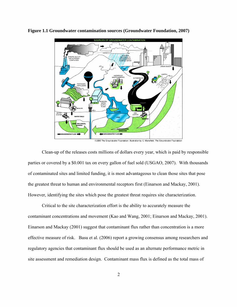
Figure 1.1 Groundwater contamination sources (Groundwater Foundation, 2007)

Clean-up of the releases costs millions of dollars every year, which is paid by responsible

parties or covered by a $0.001 tax on every gallon of fuel sold (USGAO, 2007). With thousands

of contaminated sites and limited funding, it is most advantageous to clean those sites that pose

the greatest threat to human and environmental receptors first (Einarson and Mackay, 2001).

However, identifying the sites which pose the greatest threat requires site characterization.

Critical to the site characterization effort is the ability to accurately measure the

contaminant concentrations and movement (Kao and Wang, 2001; Einarson and Mackay, 2001).

Einarson and Mackay (2001) suggest that contaminant flux rather than concentration is a more

effective measure of risk. Basu et al. (2006) report a growing consensus among researchers and

regulatory agencies that contaminant flux should be used as an alternate performance metric in

site assessment and remediation design. Contaminant mass flux is defined as the total mass of

2

3

contaminant passing a unit area of control plane that is perpendicular to the mean groundwater

flow direction per unit time (Basu et al., 2006). Mass flux is a key parameter needed to

characterize contaminant movement; it provides data that are essential to prioritizing

contaminated sites for remediation (Einarson and Mackay, 2001; USEPA, 2007). Contaminant

mass flux measurements integrated over a source area will produce estimates of the source

strength and generate critical data for optimizing design and assessing performance of source

remediation technologies (Annable et al., 2005)

Recent studies (Einarson and Mackay, 2001; USEPA, 2007; NRC, 2004; Basu et al.,

2006) have shown that contaminant mass flux is an important parameter to quantify in order to

assist remediation decision making at sites with contaminated groundwater. Mass flux

measurements may be used to 1) prioritize contaminated groundwater sites for remediation, 2)

evaluate the effectiveness of source removal technologies or natural attenuation processes, and 3)

define a source term for groundwater contaminant transport modeling, which can be used as a

tool to achieve the previous two objectives and to assist with remediation technology design

(Goltz et al., 2007a).

Current methods for measuring contaminant mass flux include the transect method (TM)

using multi-level sampling (MLS), the integral pump test (IPT, formerly known as the integral

groundwater investigation method (IGIM)), and passive flux meters (PFMs). In addition to the

above-mentioned methods, new groundwater contaminant mass flux measurement methods are

in development. The newer methods include modified integral pump tests (MIPTs) and tandem

circulating wells (TCWs). The introduction of new flux measurement methods offers the

potential of increased accuracy and decreased cost and time. The development of the new

methods has also created a knowledge gap between current field practices and the progress made

4

in academic research. In order to facilitate transfer and application of an innovative technology,

it is essential that potential technology users have access to credible information that addresses

the capabilities, limitations, and projected expenses of the new technology (NRC, 1997).

1.2 Background

The innovative flux measurement methods may be categorized by how they measure

flux. Some methods are so-called point methods, where the measurements are taken at particular

locations at particular instants in time. Other methods employ time-averaging, where samples

are taken at particular locations, but averaged over defined time intervals. Still other methods

employ a volume-averaging approach, where pumping is used to estimate flux averaged over a

large subsurface volume.

Depending on circumstances, each method has advantages and disadvantages in

comparison to the other methods. A number of studies have been conducted that have looked at

the performance of the new flux measurement technologies in both the laboratory and field

(Hatfield et al., 2004; ESTCP, 2007b; Brooks et al., 2007; Goltz et al., 2007a; 2007b; ESTCP,

2006; SERDP, 2004). Costs of applying the new technologies have been addressed to a smaller

degree. Not addressed at all is a side-by-side comparison of the different methods under varying

hydrogeologic conditions. In addition, past studies have not looked at how the choice of

measurement methodology is affected by the purpose of the measurement. As noted earlier, flux

measurement is essentially done for two reasons: (1) assess risk in order to develop cleanup

priorities or evaluate the efficacy of remediation and (2) design of a remediation technology. In

the sections below, we briefly describe each mass flux measurement method.

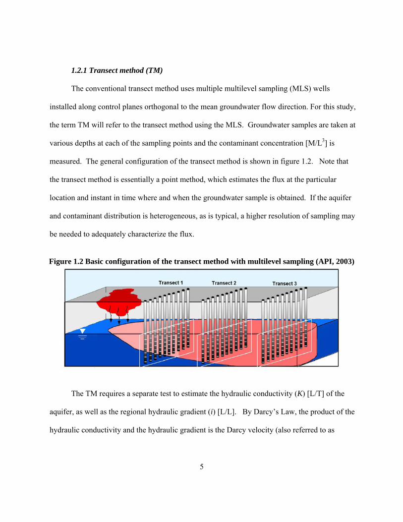
1.2.1 Transect method (TM)

The conventional transect method uses multiple multilevel sampling (MLS) wells

installed along control planes orthogonal to the mean groundwater flow direction. For this study,

the term TM will refer to the transect method using the MLS. Groundwater samples are taken at

various depths at each of the sampling points and the contaminant concentration [M/L3] is

measured. The general configuration of the transect method is shown in figure 1.2. Note that

the transect method is essentially a point method, which estimates the flux at the particular

location and instant in time where and when the groundwater sample is obtained. If the aquifer

and contaminant distribution is heterogeneous, as is typical, a higher resolution of sampling may

be needed to adequately characterize the flux.

Figure 1.2 Basic configuration of the transect method with multilevel sampling (API, 2003)

The TM requires a separate test to estimate the hydraulic conductivity (K) [L/T] of the

aquifer, as well as the regional hydraulic gradient (i) [L/L]. By Darcy’s Law, the product of the

hydraulic conductivity and the hydraulic gradient is the Darcy velocity (also referred to as

5

specific discharge or groundwater flux) (q0) [L3/L2T]. To calculate the contaminant mass flux

(J) [M/L2T], the following equation can then be used:

0J q C KiC= = − (1.1)

Slug and pump tests may be used to estimate K, while piezometers can be used to

determine the hydraulic gradient i. Another method of determining K is through the use of a

borehole dilution test (BDT). In this study, the method used in conjunction with the TM to

determine groundwater flux is the BDT test. The BDT test is a method designed to estimate a

time-averaged value of q0 at a particular point. A tracer is injected into a well and the rate at

which the tracer concentration is reduced due to dilution of the tracer by groundwater flowing

through the well is monitored (Pitrak et al., 2007). A plot of tracer concentration versus time

can be interpreted to produce an estimate of the Darcy velocity of the flowing groundwater.

1.2.2 Passive flux meter (PFM)

The PFM measures the time-averaged Darcy velocity and contaminant flux at a point in

space. This innovative method, developed by University of Florida and Purdue University

researchers (Klammler et al., 2007; Campbell et al., 2006; Annable et al., 2005; Hatfield et al.,

2004; Lee et al., 2006) uses a sorbent (e.g., granular activated carbon or GAC) impregnated with

known masses of so-called resident tracers. The sorbent is then packed in a cylindrical unit and

placed down the wells of a control plane in an aquifer to be characterized. The control plane

transect used for this method is similar to the TM used when applying the MLSs (figure 1-2)

except that the packed sorbent units are placed downwell rather than using the MLSs to obtain

samples at individual depths. As flowing groundwater passes by the PFM, the groundwater

contaminant partitions into the sorbent while the resident tracer in the sorbent is released into the 6

7

groundwater. After a specified time, the sorbent is removed from the well and analyzed to

determine the mass of contaminant captured and the mass of tracer released. The amount of

tracer released is used to estimate the groundwater Darcy velocity, averaged over the time the

PFM was in the well. Similarly, the mass of contaminant captured is used, in conjunction with

the Darcy velocity, to estimate the time-averaged contaminant concentration and contaminant

flux (Hatfield et al., 2005).

1.2.3 Modified integral pump test (MIPT)

The modified integral pump test is an innovative volume-averaging method for

estimating Darcy velocity and contaminant flux. The MIPT is a variation of an earlier method,

known as the IPT (Brooks et al., 2007; Bayer-Raich et al., 2006; Ptak et al., 2003). The IPT,

formerly called the integral groundwater investigation method (IGIM), uses concentration-time

series information from a series of pumping wells located across a control plane, along with a

separately obtained estimate of Darcy velocity, to calculate contaminant mass flux (Bockelmann

et al., 2001; Ptak et al., 2003; Bauer et al., 2004). The MIPT differs from the IPT in that the

MIPT directly obtains volume-averaged estimates of Darcy velocity and concentration by

pumping multiple wells and monitoring the hydraulic head at nearby piezometers (USEPA,

2007; Brooks et al., 2007). The differences in head that are measured as pumping is increased in

steps can be used to determine an estimate of the Darcy velocity. This, in conjunction with

sampling the wells during operation to determine the concentration of contaminant, will provide

an estimate of contaminant flux (Brooks et al., 2007).

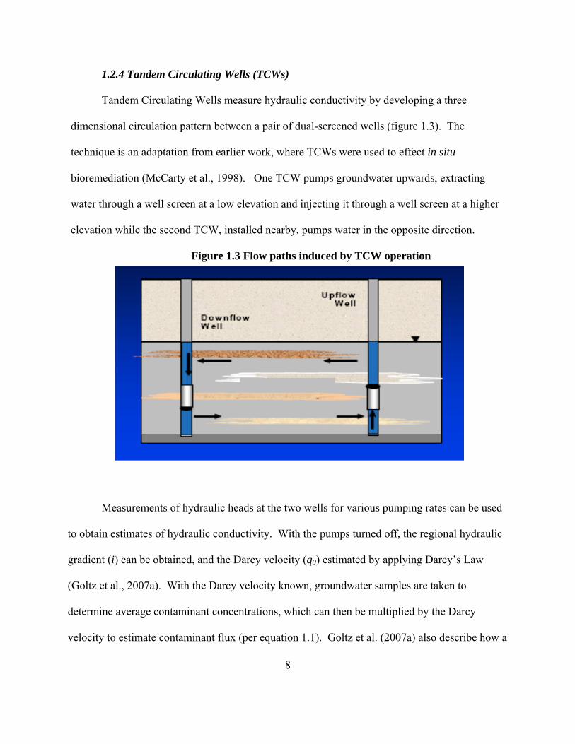
1.2.4 Tandem Circulating Wells (TCWs)

Tandem Circulating Wells measure hydraulic conductivity by developing a three

dimensional circulation pattern between a pair of dual-screened wells (figure 1.3). The

technique is an adaptation from earlier work, where TCWs were used to effect in situ

bioremediation (McCarty et al., 1998). One TCW pumps groundwater upwards, extracting

water through a well screen at a low elevation and injecting it through a well screen at a higher

elevation while the second TCW, installed nearby, pumps water in the opposite direction.

Figure 1.3 Flow paths induced by TCW operation

Measurements of hydraulic heads at the two wells for various pumping rates can be used

to obtain estimates of hydraulic conductivity. With the pumps turned off, the regional hydraulic

gradient (i) can be obtained, and the Darcy velocity (q0) estimated by applying Darcy’s Law

(Goltz et al., 2007a). With the Darcy velocity known, groundwater samples are taken to

determine average contaminant concentrations, which can then be multiplied by the Darcy

velocity to estimate contaminant flux (per equation 1.1). Goltz et al. (2007a) also describe how a

8

9

tracer test can be conducted using TCWs in order to obtain an estimate of hydraulic conductivity

(which can subsequently be used to determine Darcy velocity and contaminant flux as discussed

above).

1.3 Research Objectives

In order to facilitate transfer and application of an innovative technology, it is essential

that potential technology users have access to credible information that addresses the

capabilities, limitations, and costs of the technology. The purpose of this work is to critically

review the methods currently available to measure groundwater contaminant flux, and provide

guidelines for the implementation and use of those methods in the field.

1.4 Methodology

This study will consist of a background investigation of the aforementioned flux

measurement methods from both published and unpublished literature. When applicable,

interviews of flux measurement researchers will also be used to develop the technology review.

The review will include the following:

1. Laboratory, field, and commercial applications of conventional and innovative flux

measurement technologies. Included in the review will be:

a. A description of the measurement methods

b. Technology implementation details and costs

c. Quantification of measurements errors (accuracy, performance, etc.)

2. Information required by stakeholders to evaluate the applicability of a technology to

facilitate decision making

10

3. Cost estimation of subsurface investigation methods, considering methods for

extrapolating the results of small- and pilot-scale studies to predict full-scale costs.

Based on the literature review, we will prepare a critical analysis of the advantages and

disadvantages, costs, and measurement errors of the different methods. The analysis will include

a discussion of how hydrogeologic conditions and management objectives support application of

one method over another.

Finally, considering the requirements of decision makers that were elicited from the

literature review, we construct a “user-friendly” tool that can be used to facilitate information

transfer to potential technology users. The tool will help the technology users decide which flux

measurement method is most appropriate for given site conditions.

1.5 Study Limitations

1. Field testing

a. To date no attempt has been made to implement the TCW in the field

b. Modified IPT has not undergone validation in the field with known fluxes for

comparison

2. Cost data are limited (especially for the newer methods)

II. Literature Review

2.1 Introduction

This chapter reviews the current literature on the different flux measurement methods

briefly described in Chapter 1. We will start with a description and basic definition of flux along

with the elements required for its calculation in section 2.2. Knowing these elements will allow

us to explain the differences between the methods. Next, in section 2.3, we will systematically

describe each method, to include implementation information and a description of each method’s

advantages and disadvantages. In addition, laboratory and field tests, cost, and regulatory issues

will be reviewed for each method. In sections 2.4 and 2.5 comparisons of method performance

and costs, respectively, which have appeared in the literature, will be examined.

2.2 Mass Flux

Mass flux is the rate at which a dissolved contaminant passes through a cross-sectional

area perpendicular to the direction of flow (Basu et al., 2006). Flux therefore has units of mass

per area per time. Mass flux (J) can be calculated as the product of contaminant concentration

(C) and groundwater flux (or Darcy velocity) (q0):

0J q C= (2.1)

Since the Darcy velocity is, in accordance with Darcy’s Law, equal to the product of the

hydraulic conductivity of the porous media (K) and the hydraulic gradient (i), we may also

calculate mass flux as the product of concentration, hydraulic conductivity, and hydraulic

gradient:

J KiC= − (2.2)

11

12

Mass flux is sometimes confused with mass discharge, which has units of mass per time.

In fact, mass discharge is just the mass flux multiplied by the cross-sectional area through which

the dissolved contaminant plume is moving. Both mass discharge and mass flux are recognized

as important parameters to characterize contaminated groundwater and quantify the efficacy of

subsurface contaminant remediations (Basu et al., 2006).

Equations 2.1 and 2.2 offer different approaches to estimating contaminant mass flux.

Equation 2.1 uses q0 directly while in equation 2.2 K, i, and C are individually determined.

These parameters (q0, K, i, and C) can either be measured at a point or averaged over space

and/or time. A point measurement may not be representative of the larger cross sectional area

being considered. To decrease uncertainty, more points can be used in multiple wells at varying

depths (e.g., by using an MLS) to determine concentration and flux distribution across an area.

Though costly, this approach can provide detailed measurements of concentration and flux at

many points in a contaminant plume. A second approach is to obtain time- or space-averaged

concentration and flux measurements. This approach, in general, is less costly than a point

approach, particularly when concentrations and flux vary spatially (due, perhaps, to

heterogeneity of hydraulic conductivity or contaminant distribution) or temporally (for example,

due to hydrological fluctuations). The disadvantage of averaging is that the detailed spatial and

temporal definition of point measurements is lost.

2.3 Flux Measurement Methods

2.3.1 Transect method (TM)

The TM is a point approach to measuring concentration. From here on, TM will refer to

the transect method using the MLS unless otherwise stated. Additional tests are required to

measure K and i to calculate mass flux. Constructing the transect involves placing a control

plane perpendicular to the groundwater flow direction. Within the control plane, either

multilevel samplers or single-screen wells can be employed. To accomplish a total mass flux

calculation, it is imperative that the entire width and depth of the plume is captured by the

control plane. A transect can be placed at any distance down gradient of a contamination source.

Transects are normally placed to evaluate source strength, natural attenuation, or compliance at a

control plane. Figure 1.2 is an example of multiple transects at different locations down gradient

of a source of contamination.

The application of the transect method to determine contaminant mass flux and discharge

is relatively straightforward. Once the concentration at each of the n points across the control

plane is determined, the mass discharge, dM [M/T], at each point can be calculated by applying

equation 2.3 (API, 2003):

1

nd jj j jM C q A

== ∑ (2.3)

where Cj [M/L3] is the concentration at individual measurement point j and qj [L/T] is the

specific discharge (Darcy velocity) through the flow area associated with measurement point j

(Aj). The Aj for each measurement point j can be estimated by constructing Theissen polygons

about the points. Theissen polygons are constructed by connecting points that are located

halfway between measurement point j and adjacent measurement points. For sampling point j,

the area of the Theissen polygon around j defines Aj (Bockelmann et al., 2003).

The Darcy velocity at measurement point j (qj) can be determined directly or calculated

by Darcy’s Law:

jq Ki= − (2.4)

13

where K is the hydraulic conductivity (L/T) and i is the hydraulic gradient (L/L). In section

2.3.1.1 below, we discuss how qj, K, and i may be determined using the BDT, slug tests, and

pump tests.

To convert the mass discharge to mass flux, simply divide the total mass discharge from

equation 2.3 by the cross-sectional area of the plume across the control plane (A).

1

d df n

jj

M MMA A

=

= =∑

(2.5)

Equation 2.5 gives the average contaminant flux of the plume across the control plane.

2.3.1.1 Calculating Darcy velocity

The transect method offers the ability to measure concentrations at various points along

the transect. To complete the calculations for flux requires a value of Darcy velocity, either

measured directly or determined by Darcy’s Law (equation 2.4). The BDT provides a direct

estimate of q0 while the slug and pump test provide values for K. The hydraulic gradient is

obtained from piezometers. The difference in head measured at piezometers along the direction

of flow is divided by the distance between them to obtain the hydraulic gradient.

2.3.1.1.1The slug test

The slug test is a popular point method that is used to determine hydraulic conductivity in

both soil and rock. Slug tests are implemented by removing, adding, or displacing a known

quantity of water within a well and monitoring the changes in water level with respect to time

(Nielsen, 2006). The time it takes for the water level to reach its initial level is representative of

the horizontal hydraulic conductivity of the soil around the screened portion of the well. Data

14

15

loggers can often be used to facilitate data collection under high hydraulic conductivity

conditions where recovery takes place quickly (Nielsen, 2006). The simplest interpretation of

recovery data for hydraulic conductivity is that of Hvorslev (1951). Additionally, the Bouwer

and Rice (1976) method is also commonly used to calculate the hydraulic conductivity. For

details on conducting the slug test, refer to Nielsen (2006) or Fetter (1994).

2.3.1.1.2 The pump test

The pump test is the most popular method for investigating hydraulic properties of water-

bearing geological material (Nielsen, 2006). The test is volume-averaged and is typically

conducted using a central pumping well and one or more nearby observation wells. The

drawdown in the observation well(s) is monitored as the central well is pumped at either a

constant or variable rate. The position and configuration of the wells will depend on the aquifer

properties. Care should be taken to avoid proximity of the pumping well to boundaries (e.g.

recharging river or impervious zones). This will allow drawdown measurements to be taken

without the influence of the boundary (Nielsen, 2006). Before the pump test is started, initial

head measurements are taken at the observations well(s). These measurements will provide a

comparison for the drawdown measurements once pumping begins. Once pumping starts, the

drawdown measurements are taken and plotted for each well on a time-verses-drawdown semi

logarithmic chart. A horizontal line will indicate steady-state or near steady-state. Analysis of

the data depends on the type of aquifer and conditions. At steady-state, graphical and analytical

solutions can be applied to the well drawdown data to determine the hydraulic properties.

Details for determining hydraulic conductivity from pump tests for different aquifer conditions

may be found in Nielsen (2006).

2.3.1.1.3 Borehole dilution test (BDT)

The borehole dilution test is a time-averaged point method that is used to determine

Darcy velocity directly. The BDT is conducted by injecting a known amount of tracer into a

well and monitoring concentration levels as it dissipates due to the flow of groundwater through

the well screen (Lile et al., 1997). Salts, such as potassium bromide, are commonly used as

tracers. Concentrations of these salt tracers are easily measured by monitoring changes in

electrical conductivity or by using a specific ion electrode (USEPA, 2007). The rate at which the

tracer dissipates is a measure of the groundwater Darcy velocity. However, because the

hydraulic conductivity of the well and borehole are different than the conductivity of the aquifer

(typically the well and borehole conductivity is higher), flow lines will converge at the borehole.

The impact of this must be accounted for when calculating the Darcy velocity from BDT data.

Unfortunately, the degree of convergence (α) is difficult to quantify, resulting in either an over or

underestimate of Darcy velocity (Bernstein et al., 2007). Drost et al. (1968) and Bidaux and

Tsang (1991) have presented methods for approximating the convergence factor, α. Taking into

account the convergence factor α, q0 can be solved for directly by applying equation 2.6:

0 lno

V cqAt cα

⎡ ⎤= − ⎢ ⎥

⎣ ⎦ (2.6)

where c(t) and c0 [M/L3] are the tracer concentrations within the well at time t and initially, V

[L3] is the specific well volume, and A [L2] is the projected area of the well (Bernstein et al.,

2007). Darcy velocity can be determined by a linear plot of log concentration vs. time.

Note that the BDT method measures the sum of advective flux and diffusive flux.

Advective flux is due to the flow of the groundwater, and it is the measurement of interest.

Diffusive flux is due to Fickian diffusion of the tracer, which results from the concentration

16

17

difference between the tracer in the well and the tracer outside the well. In most cases, the

advective flux is much larger than the diffusive flux and the diffusion effect can be ignored.

However, in low conductivity and highly porous formations, where the advective flux is low,

diffusion may have an important effect on the observed tracer dilution. Not accounting for

diffusion under these low flow conditions may result in false readings of high groundwater

velocities (Bernstein et al., 2007).

2.3.1.2 TM costs

The costs associated with using the TM/BDT at a hypothetical site were evaluated

(ESTCP, 2007b). Using a transect of 10 wells at a depth of 10 feet and a vertical sampling

resolution of one foot (100 points total), the study found that costs of implementing the TM/BDT

method were $430 per linear foot of well. Details of the cost breakdown are in section 2.5. It is

important to note that the cost analysis included conducting a BDT for each of the 100 points in

order to quantify Darcy velocity. This amounted to a significant fraction of the overall cost

($160 of the $430/lf). Of course, these costs could perhaps be reduced if slug or pump tests were

used instead of the BDT, or if the BDT was used at a lower resolution.

A cost analysis developed by Kim (2005) for a template site in a confined sand aquifer

with a 200 m wide and 10 m deep plume, concluded that overall costs for implementing the TM

using the pump test would be $157,000. This cost included the installation of 9 wells, 18

contaminant sample analyses, and $2,000 for conducting the slug test.

18

2.3.1.3 TM regulatory concerns

There are no regulatory issues associated with installing MLSs to implement the TM.

However, use of BDTs or pump tests bring on regulatory concerns. The BDT typically involves

injection of a salt tracer into an aquifer. This may be of concern as bromide salts may lead to the

formation of bromates under certain conditions (Goltz et al., 1998). Recent studies have

investigated the use of other tracers (e.g., the food color “Brilliant Blue”) that could be used to

avoid the concerns of using salt tracers (Pitrak et al., 2007). The pumping test will involve the

extraction of potentially contaminated groundwater which will require proper handling and

treatment.

2.3.1.4 TM Advantages and Limitations

The main advantages of the transect method are its flexibility and simplicity. Flexibility

comes from the ability to increase or decrease the sampling resolution with little difficulty.

Being able to decrease the number of sample locations offers cost savings while the ability to

increase the number of locations allows for increased resolution or expansion of the transect

width. The spacing of monitoring points is a critical aspect of the MLS method (Guilbeault,

2005; Kubert and Finkel, 2006). An increase in spatial resolution may be required for effective

plume characterization since it has been noted that upwards of 75% of mass crossing the control

plane can pass through only 10% of the transect area (Guilbeault et al., 2005). Expansion of the

transect may be needed if it is found that more sampling wells are required to delineate the

plume boundaries (Kim, 2005). Another advantage of the method is its simplicity. The method

is well-understood and has been applied at numerous sites. Thus, finding personnel to

implement the method is relatively easy. Regulators are familiar with the method and readily

19

accept its results. When used in conjunction with the BDT or the slug test, the TM does not

require extraction and treatment of large volumes of groundwater.

The limitations of the transect method are mainly due to the fact that the concentration

measurements that are obtained using the TM are point measurements in space and time. Thus,

temporal variability (e.g., weather events) may result in an over or under estimation of flux

(Goltz et al., 2007b). Spatial heterogeneity can also cause difficulties in acquiring accurate and

representative measurements. Heterogeneity of the porous media or the contaminant distribution

will require a decrease in the spacing of the sampling points and therefore an increase in the

number of points required (Kao and Wang, 2001; Guilbeault et al., 2005; Kubert and Finkel,

2006). Kubert and Finkel (2006) propose that the TM not be used where heterogeneity requires

such a high resolution that use of an integrated pumping method would be a more cost-effective

approach. We will look at this more closely in Chapter 4.

Other advantages and limitations of the TM are associated with the use of pump, slug, or

borehole dilution tests to determine the Darcy velocity. The BDT can be conducted under a wide

variety of conditions. The technique has been refined for use in geologies varying from

unconsolidated to fractured consolidated material (Pitrak et al., 2007; Bernstein et al., 2007;

Wilson et al., 2001; Lile et al., 1997). Depending upon site heterogeneity, the method may be

applied at every MLS sampling location or at a lower spatial resolution. The accuracy of the

BDT estimate of Darcy velocity is dependent upon the degree to which the borehole and well

affect the groundwater flow field, as quantified by the convergence factor, α. Additionally,

studies show that for low conductivity and high porosity media, diffusive flux of the tracer can

be significant and must be accounted for. Ignoring tracer diffusion will result in the over

estimation of groundwater flux (Bernstein et al. 2007; Arnon et al., 2005).

20

The slug test is also a common method for estimating hydraulic conductivity. The test is

basically a point method, though the conductivity measurement is averaged over the relatively

small volume of water interrogated during the test. One of the advantages of the slug test is that

it is a short-term test. The test duration can be from less than a minute to several hours. A

shortcoming is that for high conductivity formations, drawdown may be so fast that

measurements would have to be recorded using electronic data loggers, and accuracy may be

degraded Additionally, for high conductivity formations, well screen head loss may have a

significant impact on the water-level measurements (Nielsen, 2006).

The pump test is the most common method for estimating conductivity, and it is well-

understood and accepted as a good way to make conductivity measurements. The test can run

from hours to days depending on conditions (Nielsen, 2006). In addition to the time it takes to

run a pump test, the test requires extraction of potentially contaminated groundwater that will

require treatment and disposal. This incurs additional costs.

2.3.2 Passive flux meters (PFMs)

A more recently developed device for measuring flux is the in situ passive flux meter.

The PFM is a point method which time-averages the contaminant concentration and Darcy

velocity. This method, like the transect method, requires establishing a control plane that

intercepts the contaminant plume (Hatfield et al., 2005). In contrast to the TM, which must be

supplemented by a pump test, slug test, BDT, or some other method of estimating Darcy

velocity, the PFM method simultaneously measures contaminant concentration and Darcy

velocity and therefore does not require a separate velocity measurement. The PFM is essentially

a self-contained permeable unit properly sized to fit in a screened well or borehole (Hatfield et

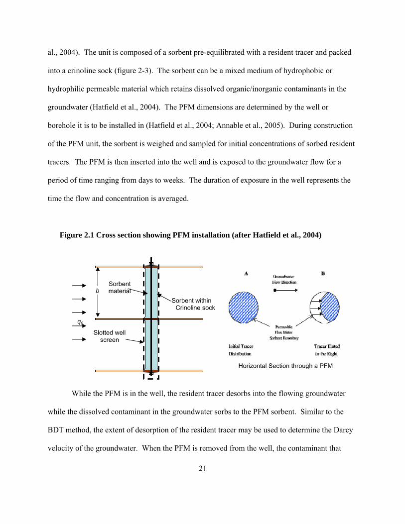
al., 2004). The unit is composed of a sorbent pre-equilibrated with a resident tracer and packed

into a crinoline sock (figure 2-3). The sorbent can be a mixed medium of hydrophobic or

hydrophilic permeable material which retains dissolved organic/inorganic contaminants in the

groundwater (Hatfield et al., 2004). The PFM dimensions are determined by the well or

borehole it is to be installed in (Hatfield et al., 2004; Annable et al., 2005). During construction

of the PFM unit, the sorbent is weighed and sampled for initial concentrations of sorbed resident

tracers. The PFM is then inserted into the well and is exposed to the groundwater flow for a

period of time ranging from days to weeks. The duration of exposure in the well represents the

time the flow and concentration is averaged.

Figure 2.1 Cross section showing PFM installation (after Hatfield et al., 2004)

21

While the PFM is in the well, the resident tracer desorbs into the flowing groundwater

while the dissolved contaminant in the groundwater sorbs to the PFM sorbent. Similar to the

BDT method, the extent of desorption of the resident tracer may be used to determine the Darcy

velocity of the groundwater. When the PFM is removed from the well, the contaminant that

Horizontal Section through a PFM

Sorbent material b

Sorbent within Crinoline sock

q0

Slotted well screen

sorbed to the sorbent, as well as the quantity of resident tracer that desorbed, are measured

(Campbell et al., 2006). The sorbed contaminant mass and desorbed resident tracer are used to

calculate a flux-averaged contaminant concentration and groundwater Darcy velocity,

respectively, at the location of the PFM. Equation 2.1 is then used to determine mass flux. By

using multiple PFMs across a control plane, an average mass flux and a total mass discharge

over the control plane may be obtained (Hatfield et al., 2005).

To determine the average groundwater specific discharge (Darcy velocity) qd [L/T]

through the PFM, without accounting for convergence or divergence of flow, apply the equation

(Hatfield et al., 2004):

1.67(1 )rd

r Rqt

dθ−Ω= (2.7)

where is the mass fraction of residual tracer remaining on the PFM after the device has been

exposed to flowing groundwater for time t, r is the radius of the borehole or well, θ is the

volumetric water content of the sorbent, and Rd is the retardation factor for the resident tracer

onto the sorbent.

rΩ

It is possible for ΩR values to fall outside the range of values (0.32-0.7) calculated

theoretically by Hatfield et al. (2004) and Basu et al. (2006) as the upper and lower limits of

residual tracer remaining to accurately calculate groundwater flux. However, it is proposed that

exceeding this theoretical range of values can be done without significant loss in accuracy, so

long as the remaining tracer mass is not excessively low (ESTCP, 2006; Hatfield et al., 2004)

To determine the ambient Darcy velocity, we must account for the convergence or

divergence of groundwater around the PFM. Since qd is linearly proportional to the ambient

groundwater flux, qo, then:

22

23

oqdq α= (2.8)

where α is the convergence/divergence factor and is a function of the difference in hydraulic

conductivity between the surrounding aquifer and that of the well and borehole. This is the same

factor discussed earlier during our explanation of the BDT calculations. Applying Equation 2.9,

the Darcy velocity can be determined:

1.67(1 )ro

r Rqt

dθα−Ω

= (2.9)

Having used the resident tracer to measure the groundwater Darcy velocity, we now use the

sorption of contaminant onto the PFM to estimate the flux-averaged dissolved contaminant

concentration. It is first necessary to measure the sorbed contaminant mass, mc. Then, the flux-

averaged contaminant concentration C [M/L3] can be estimated from Equation 2.10 (Hatfield et

al., 2004):

2c

RC DC

mCr bA Rπ θ

= (2.10)

where b is the length of the sorbent material, ARC is a dimensionless term which quantifies the

fraction of sorptive matrix containing contaminant (which can be estimated based on how much

resident tracer desorbed), θ is the volumetric water content of the sorbent, and RDC is the

retardation factor for the contaminant onto the sorbent. The time-averaged incremental

contaminant mass flux (averaged over the aquifer area interrogated by the PFM (dA) is

determined using equation 2.1. Spatial integration of the incremental measurements of

contaminant mass flux, J, yields a total time-averaged contaminant mass discharge (Md) [M/T]

across the control plane of area A:

24

odA A

M JdA q CdA= =∫ ∫ (2.11)

2.3.2.1 Laboratory and field testing of the PFM

To validate the PFM, multiple box-aquifer experiments were conducted using ethanol as

a resident tracer (Hatfield et al., 2004). These experiments measured water flux (Darcy velocity)

with relative errors of 4%. Subsequently, using 2,4 dimethyl-3-pentanol (DMP) as a

contaminant, flux (J) was calculated within 5% of known fluxes (Hatfield et al., 2004). More

recently, column tests of a new PFM configuration that used a granular anion exchange resin as

the sorbent and benzoate as the resident tracer were conducted. The granular anion exchange

resin was chosen in order to capture hexavalent chromium (Cr(VI)), an inorganic contaminant.

The contaminant was selected for study due to its high mobility and toxicity. The test, which

was also done to see if the PFM could determine the direction of groundwater flux as well as the

magnitude, measured the Darcy velocity direction with an error of 3±14º. The errors in

measuring groundwater flux magnitude and contaminant flux were -8% ±15% and -12% ± 23%,

respectively (Campbell et al., 2006).

In 2004, the PFM method was applied at a former electronic-part manufacturing facility

site that was contaminated with TCE. By using the PFM, it was determined that there were two

distinct zones, one shallow and one deep, where the groundwater flux was considerably

different: 2 cm/day and 15 cm/day in the shallow and deep zones, respectively. This finding was

significant, as previous site characterizations had not identified these zones, and the selected

remediation design did not account for them (Basu et al., 2006). Subsequent to the PFM

25

application at the site, the TM was applied and similar flux measurements were obtained (Basu et

al., 2006).

The PFM has been demonstrated at 25 sites in the US, Canada, Australia, and Wales in

an effort to gain regulatory and end-user acceptance and to stimulate transfer and

commercialization of this innovative technology (ESTCP, 2007). Field demonstrations and

comparisons with the TM/MLS were conducted at Canadian Forces Base (CFB) Borden,

NASA’s LC-34, Cape Canaveral, Florida; Naval Base Construction Base, California; and Naval

Surface Warfare Center at Indian Head, Maryland.

At CFB Borden, the PFM was compared to known (historical) groundwater fluxes as well

as fluxes measured using the BDT. These “known” fluxes were between 5 and 8 cm/day.

Deploying the PFM for 7.3 weeks, Darcy fluxes of 6.6 cm/day were measured. Also at Borden,

an experiment was conducted within a three–sided box that was constructed in the aquifer using

barrier technology. Groundwater flowed into the box at the upstream (open) end. At the

downstream end of the channel was a pumping well, pumping at 203 mL/min. Methyl tertiary

butyl ether (MTBE) was injected upstream. Within the box were three rows of three wells each.

The first row consisted of three MLS wells. The second row had three PFMs, installed without

sand packs. The third row had three PFMs with sand packs around the wells (Annable et al.,

2005). Mass discharge was measured at 0.54, 0.47, and 1.1 g/day for the MLS, PFM without

sand packs, and PFM with sand packs, respectively (Annable et al., 2005). Contaminant

(MTBE) fluxes measured by the PFMs were compared to fluxes calculated by multiplying the

induced specific discharge going into the channel by the average MTBE concentration measured

at the extraction wells and the MLSs in the channel. The results for the PFM (no sand packs)

26

were within 16.6% of the flux calculated from the MLS measurements and the PFM (sand pack)

measurements were within 1.2% of the MLSs’ (ESTCP, 2007).

NASA’s LC-34 site is contaminated with TCE due to use of the solvent in support of

rocket launch activities. An experimental flow cell was constructed at the site, consisting of

three injection and three extraction wells, along with five MLS wells within the cell. Flux

monitoring was conducted using PFMs and the MLSs before, during, and after a bioremediation

experiment at the site. The bioremediation experiment consisted of injecting ethanol as an

electron donor to stimulate biodegradation of TCE, followed by bioaugmentation, whereby

chlorinated solvent biodegrading microorganisms were injected into the aquifer. Groundwater

flux measured using the PFMs was compared to the groundwater flux that was calculated based

on flow between the injection and extraction wells. Contaminant flux measured using the PFMs

was compared to the contaminant flux estimated by applying the TM to the MLS concentration

data. In addition, contaminant mass discharge was estimated by integrating the PFM-estimated

fluxes over the flow cell cross-sectional area. This mass discharge estimate was compared to the

mass discharge measured at the extraction wells.

Prior to the bioremediation experiment, the groundwater flux measurements by the PFM

were within 6-19% of the calculated flux. After the injection of ethanol to stimulate

biodegradation, accuracy decreased, though the difference between the PFM estimate and the

calculated flux remained within 67%. Following bioremediation, the percent difference ranged

between 4 and 30% (ESTCP, 2007). It is believed that the biological activity induced during the

bioremediation resulted in some degradation of the ethanol resident tracer, resulting in the

27

observed loss of accuracy in the PFMs estimates of groundwater flux, which depend upon the

resident tracer (ESTCP, 2007).

The average contaminant flux prior to remediation was measured using both the MLS

and the PFM. Averaging over the transect planes, the difference between the PFM- and MLS-

measured fluxes prior to bioremediation ranged from 0 to 23%. During and after bioremediation,

the difference between the two methods ranged from 17 to 190%. The difference between the

mass discharge estimated by the PFM method with the “actual” discharge measured at the

extraction wells ranged from 32 to 190%. PFM estimates of vinyl chloride (VC) and ethene

fluxes (two compounds that are TCE degradation byproducts) were greater than the estimates

obtained from the MLSs and extraction wells. Project investigators speculate that TCE

degradation to VC and ethene might be occurring on the PFM sorbent, thus leading to

overestimates of VC and ethene fluxes (and an underestimate of TCE flux) (ESTCP, 2007).

At Port Hueneme, there is a contaminated site located downgradient from a Navy

Exchange Service Station. The service station reported a subsurface release of 10,800 gallons of

gasoline containing MTBE in 1984 and 1985. PFM testing was conducted in well clusters which

allowed for side-by-side comparison of PFM-measured groundwater discharges with

measurements made by the BDT and slug test methods. Although the methods were expected to

measure groundwater flux within 25%, the results varied by a factor of 2 to 3 (ESTCP, 2007).

Only the PFM was used to measure MTBE flux. However, due to natural aquifer

heterogeneities, contaminant flux measured in adjacent wells were not comparable (ESTCP,

2007)

The Indian Head site is located at the Naval Surface Warfare Center, Indian Head,

Maryland. At this facility, solid rocket propellant, containing ammonium perchlorate, was

28

cleaned out from devices such as spent rocket and ejection seat motors. This resulted in a

perchlorate plume near the facility. The groundwater gradient was 0.023 and average hydraulic

conductivity (based on slug testing) was 526 cm/day. Thus, groundwater flux based on the slug

test and the hydraulic gradient was 12 cm/day (ESTCP, 2007). In addition, groundwater flux

measured using a BDT was 3.5 cm/day (Lee et al., 2007). PFMs were installed in existing wells

with 10 ft screens. Two transects, one near the source and one further downgradient within the

plume, were established for deployment of the PFMs. Two separate deployments took place.

The first was for 3 weeks and the second for 7.3 weeks. The test focused on demonstrating the

applicability of surfactant modified silver impregnated GAC (SM-SI-GAC) in the PFM for use

in measuring groundwater and perchlorate fluxes (Lee et al., 2007; ESTCP, 2007). The

groundwater fluxes measured by the PFM for three wells were: 1.8 cm/day for MW1, 2.8 and 2.1

cm/day for MW4, and 7.6 and 4.9 cm/day for MW3. Wells MW1 and MW4 compared well to

the BDT and MW3 was within a factor of 2. The perchlorate fluxes measured at the three wells

ranged from 0.22 to 1.7 g/m2/day. Uncertainties in estimating the groundwater flow divergence

factor, as well as the proximity of well MW4 to an ongoing bioremediation study, may have

contributed to the variations in the flux measurements. The field test demonstrated that SM-SI-

GAC can be used as a sorbent for the PFM at sites with perchlorate concentrations ranging from

7 to 64 mg/L (ESTCP, 2007).

29

2.3.2.2 PFM costs

In their report, ESTCP (2007) set up a notional template site which consisted of 10 wells

spaced 10 ft apart in a transect, with each well screened over 10 ft depth in the saturated

subsurface. Thus, there was a total of 100 linear feet (lf) of screened well installed. It was

assumed that 20 five-foot long PFMs would be deployed in these wells. The vertical sampling

interval for the PFMs is assumed to be one foot; resulting in a total of 100 data points. The cost

of using the PFM to measure groundwater and contaminant flux was compared to the costs of

using the TM (with MLSs and a BDT at each MLS sampling point). The number of sampling

points for the MLS and BDT were assumed to be the same as the PFM (i.e., 100 sampling points

total). ESTCP (2007) estimated the PFM approach applied to the template site, using the one-

foot vertical resolution described above, would cost $303/lf, as compared to $430/lf for the TM.

The breakouts of the costs for the TM and PFM methods at the template site are shown in Tables

2.7 and 2.8, in section 2.5.

A cost analysis was conducted by Kim (2005) for a template site consisting of a 200 m

wide by 10 m deep contaminant plume in a confined sand aquifer. His analysis concluded the

costs for implementing the PFM method would be $155,000 or 99% of the cost of implementing

the transect method at the site (Goltz et al., 2007b). Note that the cost analysis for the PFM

method has considerable uncertainty, as only cost data to construct the PFMs and analyze the

tracer and contaminant concentrations are based upon research studies conducted at Purdue

University and the University of Florida (ESTCP, 2007; Annable et al., 2005; Basu et al., 2006).

It is unclear what costs will be once technology use is more widespread.

30

2.3.2.3 Regulatory concerns

Besides the concern that regulators may have with the accuracy of using this innovative

technology to measure groundwater contaminant flux, the only other concern might be with the

release of resident tracers into the groundwater. In some circumstances, approval to use the

resident tracer might require a permit, with the associated costs in time and money (ESTCP,

2007).

2.3.2.4 Advantages and limitations

The PFM method has no requirement for on-site electric power, making the method very

amenable for use at remote sites. PFMs are easy to install and little site labor is needed for the

duration of the test (ESTCP, 2007). The PFM also offers the same flexibility as the MLS and

becomes more economical when high spatial resolution monitoring is required (ESTCP, 2007).

In addition to contaminant and groundwater flux, the PFM can also be used to determine the

direction of groundwater flow (Campbell et al., 2004). The fact that the PFM provides a time-

averaged flux is also useful (Basu et al., 2006). Since the test duration is days to weeks long,

time-averaging avoids anomalies that may be seen from point sampling in time (Goltz et al.,

2007b). Of course, this means that a PFM measurement requires weeks, as compared with the

TM, that provides results quickly.

As a new technology, the PFM does require special expertise in selecting the appropriate

sorbent and resident tracer. As noted in the discussion of the PFM evaluation at LC-34, both the

sorbed contaminant and the resident tracer may be susceptible to bioactivity, which would skew

results (ESTCP, 2007).

31

Like the BDT, the PFM requires estimation of the convergence and divergence factor (α).

The error associated with estimating this factor directly affects the estimate of flux.

2.3.3 Tandem circulating wells (TCWs)

Goltz et al. (2007a) and Huang et al. (2004) proposed an innovative approach to

measuring contaminant mass flux through the use of tandem circulating wells (Kim, 2005). The

TCW technique uses two dual-screened wells (figure 1.3). One well extracts water from lower

depths of the aquifer and pumps the water upwards, injecting it at shallow depths, while the other

well operates in the opposite direction. This results in circulation of water between the two

wells. The extent of circulation is a function of pumping rate, hydraulic conductivity, distance

between the wells, well screen locations, and the regional hydraulic gradient. The TCW method

offers the advantage of obtaining volume-averaged measurements of contaminant concentration

(C) and hydraulic conductivity (K) by interrogating a large volume of subsurface water, without

the need to extract water from the subsurface. Knowing C and K, along with an independent

measurement of the regional hydraulic gradient (i) that can be determined by measuring the

piezometric surface at the two TCW wells (with pumps turned off) and a third piezometer,

contaminant mass flux can be calculated using equation 2.2 (Yoon, 2006; Goltz et al., 2007a).

The details of obtaining volume-averaged contaminant concentration and hydraulic conductivity

measurements are described below.

For concentration measurements, the samples are taken directly from the wells as water

circulates through them, providing a volume-averaged concentration. Calculating the hydraulic

conductivity using TCWs can be accomplished in one of two ways. One way is by application of

the multi-dipole technique (TCW-MD), which requires that the extent of drawdown (for the

downflow TCW) and mounding (for the upflow TCW) be measured for various TCW pumping

rates (Yoon, 2006). The second approach, the tracer test technique (TCW-T), uses tracers

injected in each of the two TCWs to quantify the extent of circulation (referred to as interflow)

between the two TCWs (Goltz et al., 2007a).

The multi-dipole technique is an adaptation of the single-well dipole flow test method to

simultaneously measure both horizontal and vertical hydraulic conductivity that was developed

by Kabala (1993) (Goltz et al., 2007a). To apply the method, the TCWs are operated at various

flow rates and the drawdown and mounding are measured at the downflow and upflow TCW,

respectively, for each flow rate. Goltz et al. (2004) presented a method that makes use of a

genetic algorithm to determine values for horizontal and vertical hydraulic conductivities that

result in a best fit of model-simulated (Hcalc) and measured (Hmeas) values of drawdown and

mounding. Model-simulated values of drawdown and mounding may be obtained by either

analytical (Goltz et al., 2007a) or numerical (Harbaugh and McDonald, 1996) modeling. The

best fit value for hydraulic conductivity will maximize the objective function in Equation 2.12

below.

2

1

1

1 ( )obj N

i imeas calc

i

FH H

=

=+ −∑

(2.12)

where and indicate the measured and calculated hydraulic heads at the ith flow rate,

respectively, and N is the total number of head measurements.

imeasH i

calcH

For cases where drawdown and mounding induced by the TCW are difficult to measure, due

to their relatively small magnitudes (which may occur in high hydraulic conductivity systems),

the tracer technique is an alternative method. This technique is based on determining the

32

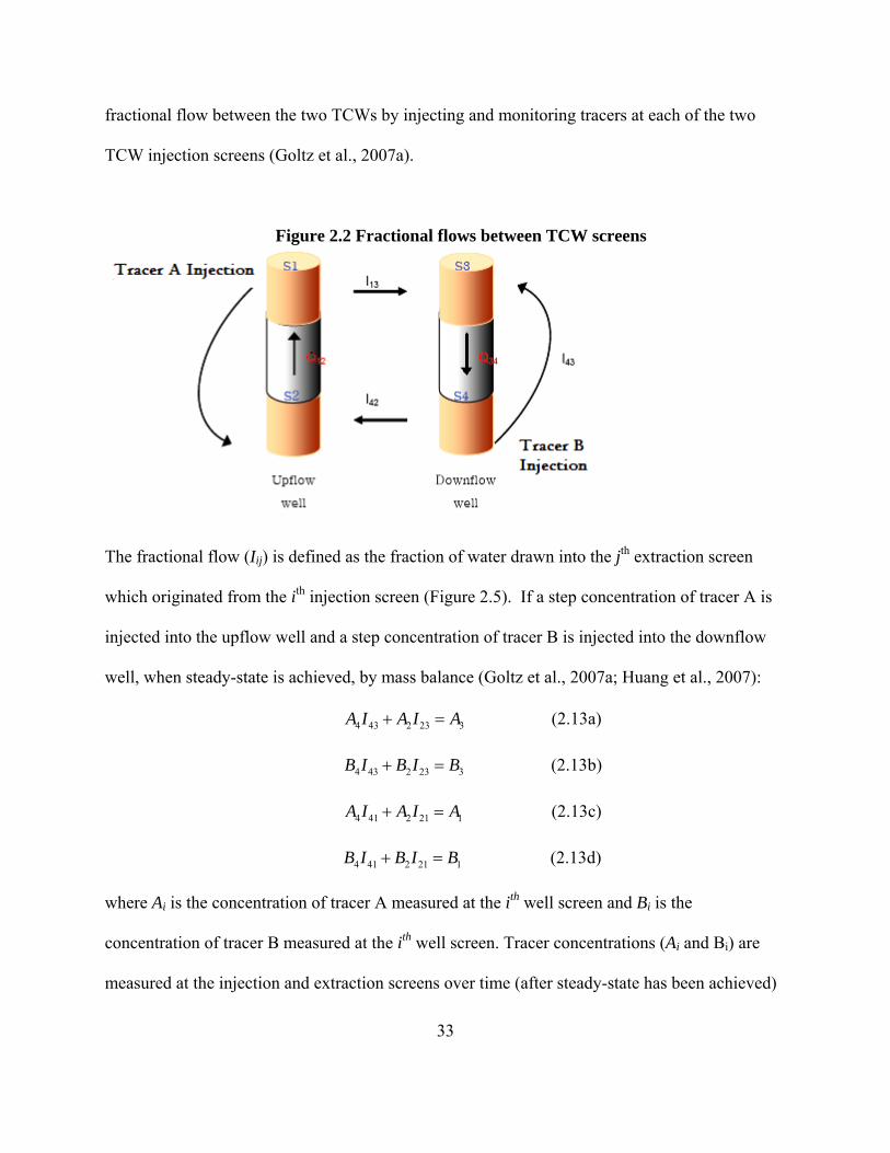
fractional flow between the two TCWs by injecting and monitoring tracers at each of the two

TCW injection screens (Goltz et al., 2007a).

Figure 2.2 Fractional flows between TCW screens

The fractional flow (Iij) is defined as the fraction of water drawn into the jth extraction screen

which originated from the ith injection screen (Figure 2.5). If a step concentration of tracer A is

injected into the upflow well and a step concentration of tracer B is injected into the downflow

well, when steady-state is achieved, by mass balance (Goltz et al., 2007a; Huang et al., 2007):

4 43 2 23 3A I A I A+ = (2.13a)

4 43 2 23 3B I B I B+ = (2.13b)

4 41 2 21 1A I A I A+ = (2.13c)

4 41 2 21 1B I B I B+ = (2.13d)

where Ai is the concentration of tracer A measured at the ith well screen and Bi is the

concentration of tracer B measured at the ith well screen. Tracer concentrations (Ai and Bi) are

measured at the injection and extraction screens over time (after steady-state has been achieved)

33

(Goltz et al, 2007). The measured concentrations may be averaged; Kim (2005) showed that the

calculation is not sensitive to the averaging method that is used.

Having values for Ai and Bi, Equation 2.13 may be solved for the four fractional flows

(Iijmeas). The numerical model MODFLOW (Harbaugh and McDonald, 1996) can then be

employed to calculate simulated values of fractional flow (Iijcalc) for the TCW flow rate used in

the test (Goltz et al., 2007a). The optimum hydraulic conductivity may then be found by using a

genetic algorithm to maximize the following objective function (Fobj):

2

1 1

1

1 (inj ext

obj N Nmeas calcij ij

i j

FI I

= =

=+ −∑∑ )

(2.14)

where Nij and Next are the number of injection and extraction well screens, respectively, and N is

the total number of well screens.

2.3.3.1 Laboratory testing of the TCW

TCW laboratory experiments were conducted in Canterbury, New Zealand, in a large

“meso-scale”, homogeneous sand aquifer. The aquifer was 9.5 m long, 4.7 m wide, and 2.6 m

deep and filled with sifted sand ranging in size from 0.6 to 1.2 mm in diameter. Constant head

tanks at either end of the aquifer provided a “regional” hydraulic gradient (Goltz et al., 2007a).

The target contaminant was chloride which was naturally present in the water. The actual mass

flux was calculated by multiplying the chloride concentration in the influent water by the flow

through the aquifer and dividing by the cross-sectional area. Both the tracer and multi-dipole

approaches were tested, and the results were compared with the TM. The results of the

experiments show relatively accurate results for the multi-dipole approach and for the tracer

34

35

approach. Goltz et al. (2007a) report the multi-dipole approach estimated a hydraulic

conductivity of 173 m/d. The measured hydraulic gradient was 0.00132 and contaminant

concentration was 10.5 g/m3. Applying equation 2.2, the estimated mass flux was 2.39 g/m2/d.

This compares very well with the actual flux of 2.41 g/m2/d.

The tracer test used bromide injected into the injection screen of the upflow well and

nitrate injected into the injection screen of the downflow well. The bromide and nitrate

injections continued for 240 and 336 hours, respectively, until steady-state concentrations were

reached at the extraction wells (Goltz et al., 2007a). Values for the hydraulic conductivity were

obtained by applying equations 2.13 and 2.14. The TCW tracer test resulted in a flux estimate of

2.53 g/m2/d, 13% greater than the actual flux. Unfortunately, although TCWs have been used in

the field to implement in situ remediation (McCarty et al., 1998), TCWs have never been

implemented to measure contaminant mass flux in the field.

2.3.3.2 TCW Costs

Kim (2005) estimated the costs of measuring flux at a template site using the TCW (see

template site description in Section 2.5). He calculated that the multi-dipole approach would

cost $84,000 and the tracer approach would cost $92,000. The cost estimates assumed

installation of two 8-inch wells plus a single 2-inch piezometer. The tracer test was conducted

for 12.5 days. The cost of the multi-dipole and tracer approach equated to 54% and 59%,

respectively, of the costs associated with implementing the TM with a single pump test for

estimating hydraulic conductivity.

36

2.3.3.3 TCW regulatory concerns

The TCW tracer method requires the use of tracers which may raise some regulatory

concerns (Goltz et al., 2007b) and may require permitting. There is also the issue of possible

contamination of clean groundwater due to circulating water between the lower and upper depths

of an aquifer. Additionally, the fact that the technology has never been field-tested will probably

lead regulators to question its accuracy.

2.3.3.4 TCW Advantages and limitations

The inherent advantage of the TCW method is that it is a volume-averaged approach,

eliminating the need for the extensive sampling (and associated costs) that is required when

applying point measurements in heterogeneous systems (USEPA, 2007). The TCW method

avoids the extraction and treatment of contaminated groundwater (Goltz et al., 2007a). Since the

TCW method does not require that groundwater be pumped to the surface, the test is economical

when characterizing deep plumes (Goltz et al., 2004). The TCW method can be of greater value

if conditions do not allow for the installation of many wells for a large control plane due to

geologic conditions or surface obstructions.

Although the TCW technique has been used in the past for remediation of contaminant

plumes, it has not been applied in the field to measure flux (Yoon, 2006). Depending on

hydraulic conductivity, pumping rate, and distance between the TCWs, the tracer technique may

require a relatively long time (perhaps weeks) to establish steady-state tracer concentrations

(USEPA, 2007). Another disadvantage is that the calculations for determining the flux (e.g.,

application of a genetic algorithm to estimate hydraulic conductivity) can be rather complex

(USEPA, 2007).

37

2.3.4 Modified Integral Pump Tests (MIPTs)

Like the TCW method, the MIPT method obtains a volume-averaged measurement by

interrogating a large volume of subsurface water (Brooks et al., 2007). The MIPT is a simplified

version of the IPT, requiring less time to implement and therefore having the potential to reduce

costs associated with labor and disposal of extracted water.

The original IPT was introduced as a flux measurement technique by Teutsch et al.

(2000). To apply the IPT to measure flux, one or more pumping wells are installed along a

control plane down gradient of a contamination source and orthogonal to the regional

groundwater flow direction (Brooks et al., 2005; SERDP, 2004). Enough wells are installed to

ensure capture of the entire contaminant plume (Bockelmann et al., 2001). The wells are

pumped simultaneously or sequentially for several days and contaminant concentration measured

as a function of time (Ptak et al., 2003). This concentration-time series information is used to

estimate average contaminant concentration based on a number of assumptions: (1) flow towards

the extraction wells is radially symmetric and regional flow can be ignored during the pumping

test, (2) the aquifer is homogeneous with regard to porosity, hydraulic conductivity, and

thickness, and (3) the concentration does not vary significantly within each streamtube at the

scale of the well capture zone (Goltz et al., 2007b; Bockelmann et al. 2001). Hydraulic

conductivity and gradient are measured separately, and Equations 2.2 and 2.3 are then used to

estimate contaminant mass flux and mass discharge, respectively (Bockelmann et al., 2003).

The IPT has had several field implementations at various European industrial areas

(megasites) to include Strausbourg, Linz, Stuttgart, and Milano. It was concluded that the IPT

was capable of quickly and with certainty estimating the average contaminant concentration,

spatial distribution of concentration, and mass discharge of contaminant down gradient of a

source (Ptak et al., 2003).

The MIPT method also uses pumping wells, along with monitoring wells, to measure

flux. The basis of the MIPT method is to determine the regional Darcy velocity, q0, by

measuring the head difference between the pumping wells and the monitoring well(s), when the

pumping wells are pumped at different flow rates. If we assume a homogeneous confined

aquifer of saturated thickness B and steady flow, the head difference between the pumping well

at the origin and the monitoring well a distance Δx directly downgradient (Figure 2.5) can be

expressed as a function of the sum of the flows in each of N pumping wells (Qi as i goes from 1

to N) (Yoon, 2006; USEPA, 2007).

2[ ]0

21 [ ]

1 ln4

Nobs i

ii w i

rq Bh x QT T rπ =

Δ = − Δ + ∑ (2.15)

where robs[i] is the distance to the observation well from the ith pumping well, rw[i] is the distance

between the ith pumping well and the origin, and T is the aquifer transmissivity, which is the

hydraulic conductivity multiplied by the aquifer saturated thickness. The head differences are

measured at different pumping rates, and plotted against the summation term on the right-hand-

side of Equation 2.15. A best-fit line is constructed from the Δh versus 2

[ ]2

1 [ ]

lnN

obs ii

i w i

rQ

r=∑ data. The

line crosses the x-axis when Δh = 0. The value of 2

[ ]2

1 [ ]

lnN

obs ii

i w i

rQ

r=∑ at the x-axis intercept allows

calculation of the regional Darcy velocity, q0, using equation 2.16:

2[ ]

0 21 [ ] 0

1 ln4

Nobs i

ii w i x

rq Q

B x rπ = =

⎡ ⎤= ⎢ ⎥

Δ ⎢ ⎥⎣ ⎦∑ (2.16)

38

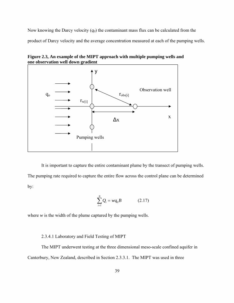
Now knowing the Darcy velocity (q0) the contaminant mass flux can be calculated from the

product of Darcy velocity and the average concentration measured at each of the pumping wells.

Figure 2.3, An example of the MIPT approach with multiple pumping wells and one observation well down gradient

qo

x

Pumping wells

Observation well

y

Δx

robs[i]

rw[i]

It is important to capture the entire contaminant plume by the transect of pumping wells.

The pumping rate required to capture the entire flow across the control plane can be determined

by:

01

N

ii

Q wq B=

=∑ (2.17)

where w is the width of the plume captured by the pumping wells.

2.3.4.1 Laboratory and Field Testing of MIPT

The MIPT underwent testing at the three dimensional meso-scale confined aquifer in

Canterbury, New Zealand, described in Section 2.3.3.1. The MIPT was used in three

39

40

experiments. In each experiment, the pumping wells were pumped at 5 different rates and head

measurements made for each rate. Experiments 1 and 3 employed a single pumping well and

experiment 2 employed three pumping wells. Experiments 1, 2, and 3 under estimated the actual

flux by 48, 42, and 61% respectively (Goltz et al., 2007b).

The MIPT was fielded at a contaminated site at Hill AFB, Utah, where degreasing

solvents, primarily TCE, had been released (Brooks et al., 2007). The site has been undergoing

remediation since the early 1990s. Before and after a source remediation effort in July 2002, the

MIPT was used to measure the contaminant flux change that resulted from the remediation.

Prior to the remediation effort, a transect of 10 wells spaced 10 feet apart was installed. The

primary contaminants in the groundwater were TCE and DCE. During the pre-remediation test,

4 pumping steps were applied; for the first post remediation test, three steps were used; while for

the second post remediation test, 5 steps were used (Brooks et al., 2007). Groundwater samples

were taken at 3 to 6 hour intervals during each MIPT. Hydraulic gradients were measured before

all the tests. Using historical data from previous studies (Meinardus et al., 2002; Rao et al.,

1997), the hydraulic conductivity was estimated at 17 m/d (Brooks et al., 2007). Applying

Equation 2.4, Darcy velocities of 3.4, 3.4, and 0.9 cm/day were estimated for each of the three

tests. Although the actual contaminant mass flux was not known, the test results were compared

to results obtained from the TM, which used previously measured values for hydraulic

conductivity and gradient (see equation 2.2). Based on the TM, transect-wide average Darcy

fluxes of 2.9, 1.7, and 3.2 cm/day were measured for the pre-remediation and two post-

remediation tests, respectively. This compares well with the groundwater flux estimated from

previously reported hydraulic conductivity and hydraulic gradient measurements. Based on the

MIPTs and measured hydraulic gradients, the following values of hydraulic conductivity were

41

calculated for each of the three tests: 19.0, 12.0, and 18.0 m/day. These three estimates of

hydraulic conductivity are averaged to obtain a value of 16 m/day, with a standard deviation of

0.40 m/day. This compares reasonably well with previously published estimates (Brooks et al.,

2007).

TCE mass discharge measurements using the MIPT yielded values of 76, 3.9, and 7.1

g/day for pre-remediation, first post-remediation, and second post-remediation tests,

respectively. Also measured was DCE mass discharge of 2.0 and 20 g/day for the first and

second post-remediation tests, respectively. This compares with TCE mass discharge

measurements using the transect approach of 78, 7.2, and 1.3 g/day for the pre-remediation, first

post-remediation, and second post-remediation tests, respectively, and DCE mass discharge

measurements of 3.8 and 4.2 g/day for the two post-remediation tests (Brooks et al., 2007). The

PFM was also tested at the site. Comparison of the PFM and MIPT methods is discussed in

Section 2.4.

At the Fort Lewis, Washington, East Gate Disposal Yard, a release of chlorinated

solvents (mostly TCE) had occurred from drums. The TCE plume is well established and

extends north for approximately 4 kilometers. A pump-and-treat system was installed in 1995

for hydraulic control purposes and the drums were removed in 2000 and 2001 (Brooks et al.,

2007). In 2003, thermal treatment was used to treat the source area. Before (Phase I) and after

(Phase II) the thermal treatment, the MIPT was used to measure flux. Hydraulic gradients were

measured during each of the two MIPTs. The MIPT used 10 wells spaced along a 60 m transect.

During Phase I, the MIPT pumping rates were not large enough to stress the aquifer for sufficient

drawdown, so groundwater flux was not directly measured. However, after Phase II was

complete, the Phase I flux was estimated by scaling the Phase II estimated groundwater flux by

42

using the ratio of hydraulic gradients of the two phases. The resulting groundwater fluxes were

then estimated to be 32 and 18 cm/day for Phases I and II, respectively (Brooks et al., 2007).

This compares well with the 34 and 19 cm/day estimates that were made based on multiplying

the measured hydraulic gradients by the average hydraulic conductivity at the site.

Based on the MIPT-measured groundwater fluxes, the TCE mass discharge was

calculated at 536 and 2.2 g/day for pre- and post-remediation tests, and the DCE discharge

calculated at 257 g/day for the pre-remediation test (DCE was not detected in the post-

remediation sample analysis). These mass discharge estimates compared well with pre-

remediation estimates made using the TM of 688 g/day for TCE and 288 g/day for DCE. The

post-remediation measurement from the MIPT for TCE (2.2 g/day) also compared well with the

estimate made using the TM (2.8 g/day) (Brooks et al., 2007). A summary of the mass discharge

measurements at Fort Lewis may be seen in Table 2.1 in section 2.4.

Field tests of the MIPT method have also been conducted at a tetrachloroethylene (PCE)-

contaminated dry-cleaning site in Jacksonville, FL, and a dense nonaqueous phase liquid

(DNAPL) spill site at Canadian Forces Base Borden. However, neither the Jacksonville nor

Borden site data have been published.

2.3.4.2 MIPT costs

There were no cost data found in literature. In Chapter 3, we develop a cost estimation

methodology for the MIPT method, which is subsequently applied in Chapter 4.

2.3.4.3 MIPT Regulatory issues

The extraction of potentially contaminated groundwater is of regulatory concern.

43

2.3.4.4 MIPT Advantages and limitations

Like the TCW method, the MIPT method obtains a volume-averaged measurement, thus

eliminating the need for the large number of sampling points which would be required to

characterize a heterogeneous site (SERDP, 2004). The fact that the MIPT is an active

measurement method enables varying the pumping rates to accommodate seasonal variations in

groundwater flow (Brooks et al., 2007). MIPT measurements have been shown to be consistent

with the PFM and TM methods (Brooks et al, 2006; SERDP, 2004).

In the MIPT, it is assumed that hydraulic steady-state is attained after pumping for 24

hours. The validity of this assumption will be site dependent. In addition to labor costs, the

extracted contaminated water must be treated and properly disposed of. This could increase

costs significantly; depending on location and site conditions, disposal costs can be as high as

$1/gal of extracted water (USEPA, 2007). Additionally, in order to obtain a steady concentration

measurement, pumping on the order of weeks to months may be required (USEPA, 2007).

Recently, modifications to the MIPT are being tested, with the goal of reducing the duration of

pumping (and therefore, reducing labor costs, as well as the costs associated with treating and

disposing of potentially contaminated groundwater) (SERDP, 2004).

44

2.4 Method comparison

Some comparisons where the different methods were applied at the same location and

time have appeared in the literature. Brooks et al. (2006; 2007) compared the TM with the MIPT

and PFM methods at Fort Lewis and Hill AFB. Although the actual flux was unknown,

application of the MIPT and PFM methods resulted in estimated fluxes that were within 8 to

38% of the TM estimate at Fort Lewis and within 15 to 40% of the TM estimate at Hill AFB. In

reference to the accuracy of application of the MIPT method at Hill AFB (see Section 2.3.4.1),

Brooks et al. (2006) has stated:

… it can be generally concluded that the uncertainty estimates as presented [Hill AFB] are comparable. Furthermore, in the work by Kubert and Finkel (2006), for a system comparable to the Hill AFB, transect error estimates associated with mass discharge were in the range of 15 to 40%. …Thus the conclusion that these methods are in general agreement is valid.

Table 2.1 reports results from the Hill AFB and Fort Lewis field tests, where the PFM, MIPT,

and TM were applied to measure contaminant mass discharge.

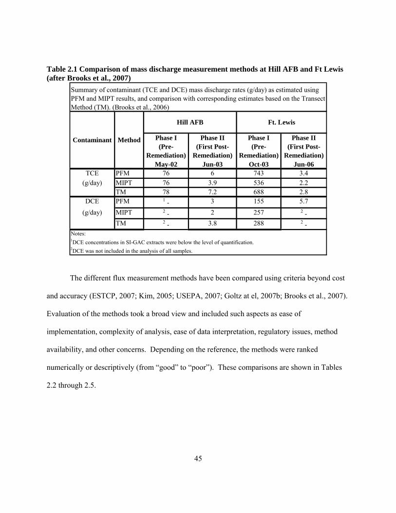
Table 2.1 Comparison of mass discharge measurement methods at Hill AFB and Ft Lewis (after Brooks et al., 2007)

Phase I Phase II Phase I Phase II(Pre-

Remediation)(First Post-

Remediation)(Pre-

Remediation)(First Post-

Remediation)May-02 Jun-03 Oct-03 Jun-06

TCE PFM 76 6 743 3.4(g/day) MIPT 76 3.9 536 2.2

TM 78 7.2 688 2.8DCE PFM 1 - 3 155 5.7

(g/day) MIPT 2 - 2 257 2 -TM 2 - 3.8 288 2 -

Notes: 1DCE concentrations in SI-GAC extracts were below the level of quantification.2DCE was not included in the analysis of all samples.

Summary of contaminant (TCE and DCE) mass discharge rates (g/day) as estimated using PFM and MIPT results, and comparison with corresponding estimates based on the Transect Method (TM). (Brooks et al., 2006)

Contaminant Method

Hill AFB Ft. Lewis

The different flux measurement methods have been compared using criteria beyond cost

and accuracy (ESTCP, 2007; Kim, 2005; USEPA, 2007; Goltz at el, 2007b; Brooks et al., 2007).

Evaluation of the methods took a broad view and included such aspects as ease of

implementation, complexity of analysis, ease of data interpretation, regulatory issues, method

availability, and other concerns. Depending on the reference, the methods were ranked

numerically or descriptively (from “good” to “poor”). These comparisons are shown in Tables

2.2 through 2.5.

45

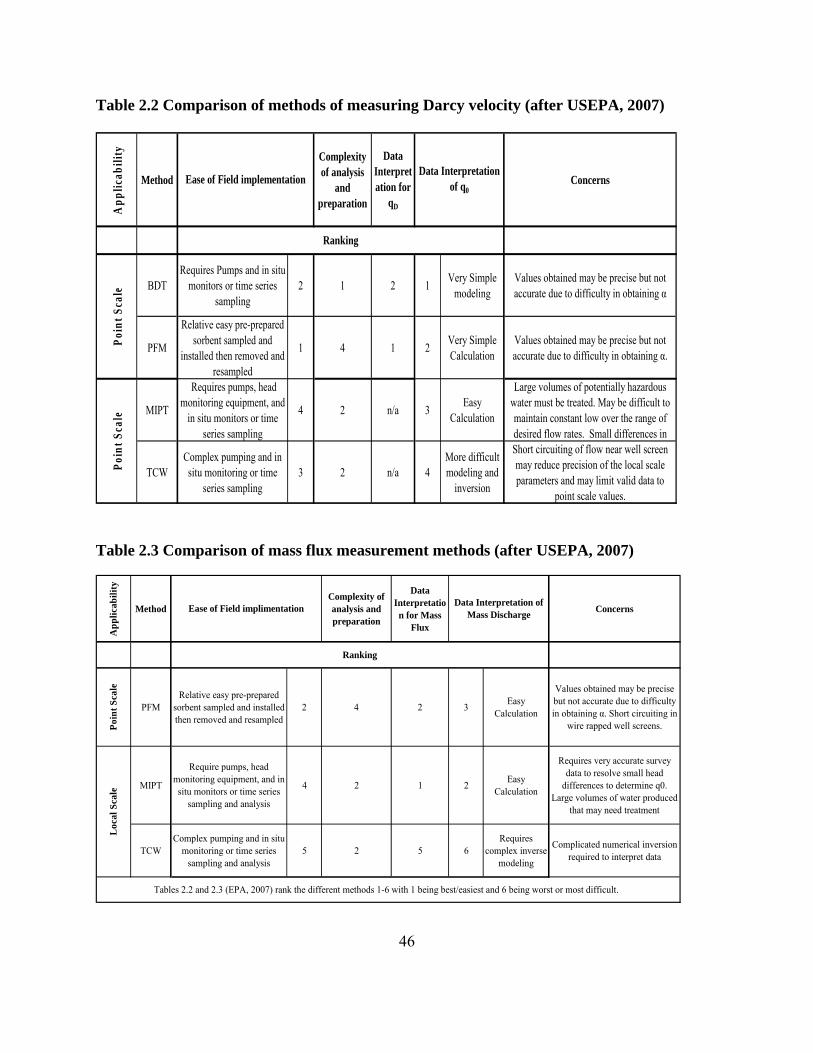
Table 2.2 Comparison of methods of measuring Darcy velocity (after USEPA, 2007) A

pplic

abili

ty

Method

Complexity of analysis

and preparation

Data Interpretation for

qD

Concerns

BDTRequires Pumps and in situ

monitors or time series sampling

2 1 2 1 Very Simple modeling

Values obtained may be precise but not accurate due to difficulty in obtaining α

PFM

Relative easy pre-prepared sorbent sampled and

installed then removed and resampled

1 4 1 2 Very Simple Calculation

Values obtained may be precise but not accurate due to difficulty in obtaining α.

MIPT

Requires pumps, head monitoring equipment, and

in situ monitors or time series sampling

4 2 n/a 3 Easy Calculation

Large volumes of potentially hazardous water must be treated. May be difficult to maintain constant low over the range of desired flow rates. Small differences in

TCWComplex pumping and in situ monitoring or time

series sampling3 2 n/a 4

More difficult modeling and

inversion

Short circuiting of flow near well screen may reduce precision of the local scale parameters and may limit valid data to

point scale values.

Poin

t Sca

le

Ease of Field implementationData Interpretation

of q0

Poin

t Sca

le

Ranking

Table 2.3 Comparison of mass flux measurement methods (after USEPA, 2007)

App

licab

ility

MethodComplexity of analysis and preparation

Data Interpretation for Mass

Flux

Concerns

PFMRelative easy pre-prepared

sorbent sampled and installed then removed and resampled

2 4 2 3 Easy Calculation

Values obtained may be precise but not accurate due to difficulty in obtaining α. Short circuiting in

wire rapped well screens.

MIPT

Require pumps, head monitoring equipment, and in situ monitors or time series

sampling and analysis

4 2 1 2 Easy Calculation

Requires very accurate survey data to resolve small head

differences to determine q0. Large volumes of water produced

that may need treatment

TCWComplex pumping and in situ

monitoring or time series sampling and analysis

5 2 5 6Requires

complex inverse modeling

Complicated numerical inversion required to interpret data

Loc

al S

cale

Tables 2.2 and 2.3 (EPA, 2007) rank the different methods 1-6 with 1 being best/easiest and 6 being worst or most difficult.

Ease of Field implimentation Data Interpretation of Mass Discharge

Poin

t Sca

le

Ranking

46

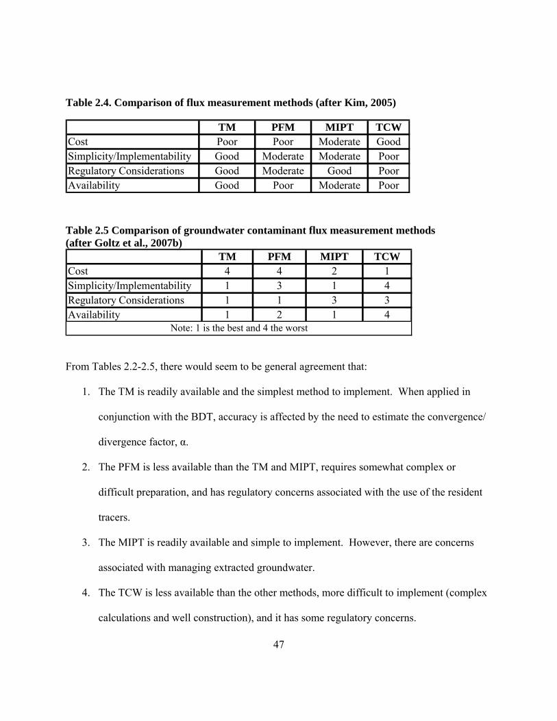
Table 2.4. Comparison of flux measurement methods (after Kim, 2005)

TM PFM MIPT TCWCost Poor Poor Moderate GoodSimplicity/Implementability Good Moderate Moderate PoorRegulatory Considerations Good Moderate Good PoorAvailability Good Poor Moderate Poor

Table 2.5 Comparison of groundwater contaminant flux measurement methods (after Goltz et al., 2007b)

TM PFM MIPT TCWCost 4 4 2 1Simplicity/Implementability 1 3 1 4Regulatory Considerations 1 1 3 3Availability 1 2 1 4

Note: 1 is the best and 4 the worst

From Tables 2.2-2.5, there would seem to be general agreement that:

1. The TM is readily available and the simplest method to implement. When applied in

conjunction with the BDT, accuracy is affected by the need to estimate the convergence/

divergence factor, α.

2. The PFM is less available than the TM and MIPT, requires somewhat complex or

difficult preparation, and has regulatory concerns associated with the use of the resident

tracers.

3. The MIPT is readily available and simple to implement. However, there are concerns

associated with managing extracted groundwater.

4. The TCW is less available than the other methods, more difficult to implement (complex

calculations and well construction), and it has some regulatory concerns.

47

48

2.5 Cost studies

The different flux measurement methods have considerable variation in cost and

comparing costs between methods is not straightforward. According to the NRC (1997), for a

variety of reasons, developing accurate cost comparisons is complicated and extremely difficult.

The leading reasons for these difficulties are:

1. Costs reported under a set of conditions at one site are very difficult to

extrapolate to another.

2. Vendors may report costs using a variety of metrics that cannot be directly

compared.

3. Technology providers do not always report all costs (such as the costs for

permitting and mobilization). They tend only to report the costs associated with

operating the system.

4. The category of cost that is reported can vary (e.g. reporting life cycle cost versus

initial capital cost).

The inherent uncertainties associated with investigating the subsurface present challenges

to comparing costs. Investigating sites is expensive and site characterization and selection of a

remediation technology can exceed the cost of the actual remediation (RS Means, 2003). To

overcome these challenges, certain steps can be employed to help evaluate and compare

technology options. One such step is to develop site templates that can be used to compare the

costs of implementing different site characterization or remediation technologies (NRC, 1997).

Another is to report costs in comparable units. The NRC (1997) suggests using template sites

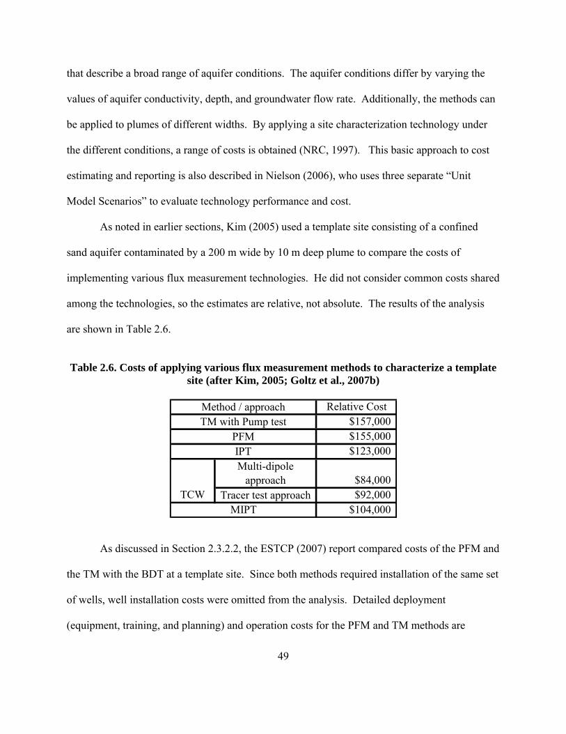
that describe a broad range of aquifer conditions. The aquifer conditions differ by varying the

values of aquifer conductivity, depth, and groundwater flow rate. Additionally, the methods can

be applied to plumes of different widths. By applying a site characterization technology under

the different conditions, a range of costs is obtained (NRC, 1997). This basic approach to cost

estimating and reporting is also described in Nielson (2006), who uses three separate “Unit

Model Scenarios” to evaluate technology performance and cost.

As noted in earlier sections, Kim (2005) used a template site consisting of a confined

sand aquifer contaminated by a 200 m wide by 10 m deep plume to compare the costs of

implementing various flux measurement technologies. He did not consider common costs shared

among the technologies, so the estimates are relative, not absolute. The results of the analysis

are shown in Table 2.6.

Table 2.6. Costs of applying various flux measurement methods to characterize a template

site (after Kim, 2005; Goltz et al., 2007b)

Relative Cost$157,000$155,000$123,000

Multi-dipole approach $84,000

Tracer test approach $92,000$104,000MIPT

TCW

Method / approachTM with Pump test

PFMIPT

As discussed in Section 2.3.2.2, the ESTCP (2007) report compared costs of the PFM and

the TM with the BDT at a template site. Since both methods required installation of the same set

of wells, well installation costs were omitted from the analysis. Detailed deployment

(equipment, training, and planning) and operation costs for the PFM and TM methods are

49

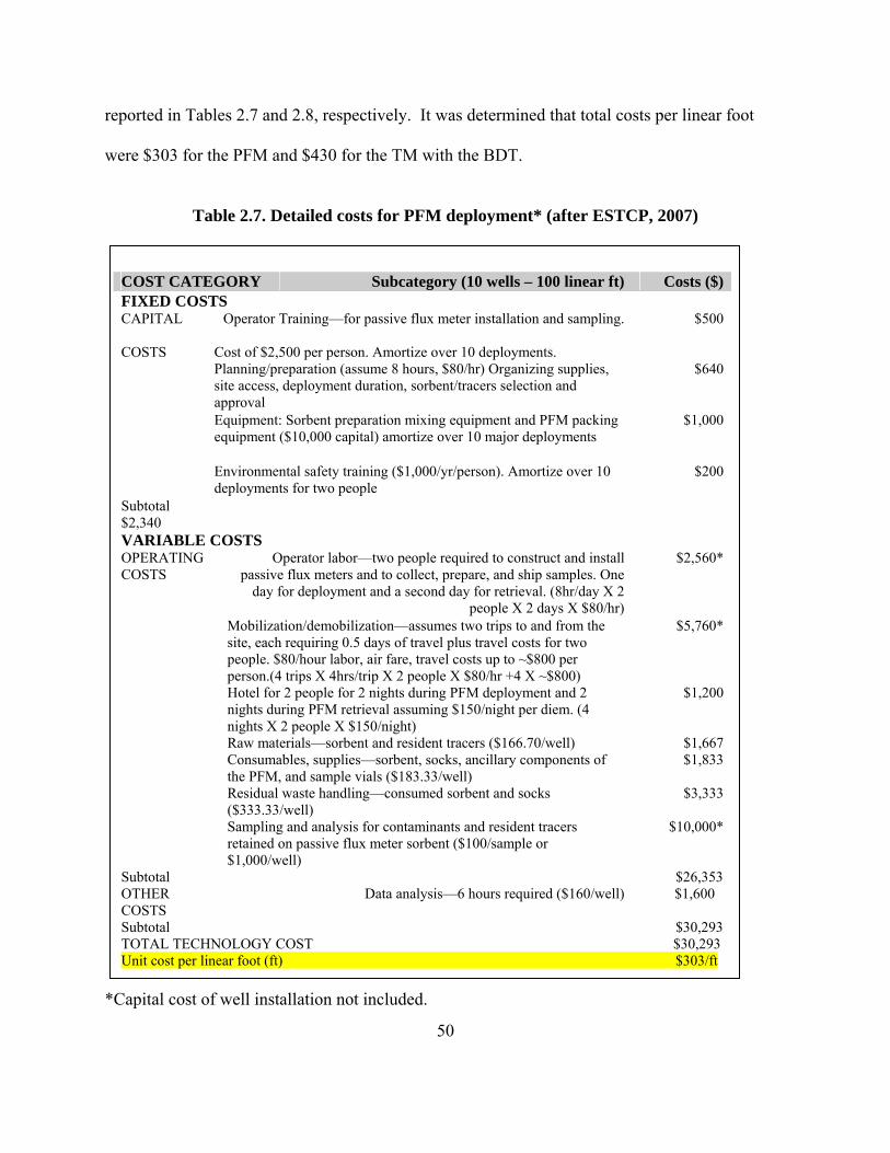
reported in Tables 2.7 and 2.8, respectively. It was determined that total costs per linear foot

were $303 for the PFM and $430 for the TM with the BDT.

Table 2.7. Detailed costs for PFM deployment* (after ESTCP, 2007)

50

*Capital cost of well installation not included.

COST CATEGORY Subcategory (10 wells – 100 linear ft) Costs ($) FIXED COSTS CAPITAL Operator Training—for passive flux meter installation and sampling. $500 COSTS Cost of $2,500 per person. Amortize over 10 deployments.

Planning/preparation (assume 8 hours, $80/hr) Organizing supplies, site access, deployment duration, sorbent/tracers selection and approval

$640

Equipment: Sorbent preparation mixing equipment and PFM packing equipment ($10,000 capital) amortize over 10 major deployments

$1,000

Environmental safety training ($1,000/yr/person). Amortize over 10 deployments for two people

$200

Subtotal $2,340 VARIABLE COSTS OPERATING COSTS

Operator labor—two people required to construct and install passive flux meters and to collect, prepare, and ship samples. One

day for deployment and a second day for retrieval. (8hr/day X 2 people X 2 days X $80/hr)

$2,560*

Mobilization/demobilization—assumes two trips to and from the site, each requiring 0.5 days of travel plus travel costs for two people. $80/hour labor, air fare, travel costs up to ~$800 per person.(4 trips X 4hrs/trip X 2 people X $80/hr +4 X ~$800)

$5,760*

Hotel for 2 people for 2 nights during PFM deployment and 2 nights during PFM retrieval assuming $150/night per diem. (4 nights X 2 people X $150/night)

$1,200

Raw materials—sorbent and resident tracers ($166.70/well) $1,667 Consumables, supplies—sorbent, socks, ancillary components of the PFM, and sample vials ($183.33/well)

$1,833

Residual waste handling—consumed sorbent and socks ($333.33/well)

$3,333

Sampling and analysis for contaminants and resident tracers retained on passive flux meter sorbent ($100/sample or $1,000/well)

$10,000*

Subtotal $26,353 OTHER COSTS

Data analysis—6 hours required ($160/well) $1,600

Subtotal $30,293 TOTAL TECHNOLOGY COST $30,293 Unit cost per linear foot (ft) $303/ft

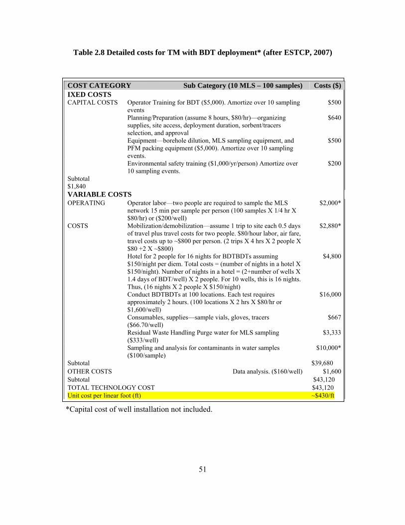
Table 2.8 Detailed costs for TM with BDT deployment* (after ESTCP, 2007)

COST CATEGORY

51

*Capital cost of well installation not included.

Sub Category (10 MLS – 100 samples) Costs ($) IXED COSTS

Operator Training for BDT ($5,000). Amortize over 10 sampling events

$500 CAPITAL COSTS

Planning/Preparation (assume 8 hours, $80/hr)—organizing supplies, site access, deployment duration, sorbent/tracers selection, and approval

$640

Equipment—borehole dilution, MLS sampling equipment, and PFM packing equipment ($5,000). Amortize over 10 sampling events.

$500

Environmental safety training ($1,000/yr/person) Amortize over 10 sampling events.

$200

Subtotal $1,840 VARIABLE COSTS

Operator labor—two people are required to sample the MLS network 15 min per sample per person (100 samples X 1/4 hr X $80/hr) or ($200/well)

$2,000* OPERATING

Mobilization/demobilization—assume 1 trip to site each 0.5 days of travel plus travel costs for two people. $80/hour labor, air fare, travel costs up to ~$800 per person. (2 trips X 4 hrs X 2 people X $80 +2 X ~$800)

$2,880* COSTS

Hotel for 2 people for 16 nights for BDTBDTs assuming $150/night per diem. Total costs = (number of nights in a hotel X $150/night). Number of nights in a hotel = (2+number of wells X 1.4 days of BDT/well) X 2 people. For 10 wells, this is 16 nights. Thus, (16 nights X 2 people X $150/night)

$4,800

Conduct BDTBDTs at 100 locations. Each test requires approximately 2 hours. (100 locations X 2 hrs X $80/hr or $1,600/well)

$16,000

Consumables, supplies—sample vials, gloves, tracers ($66.70/well)

$667

Residual Waste Handling Purge water for MLS sampling ($333/well)

$3,333

Sampling and analysis for contaminants in water samples ($100/sample)

$10,000*

Subtotal $39,680 OTHER COSTS Data analysis. ($160/well) $1,600 Subtotal $43,120 TOTAL TECHNOLOGY COST $43,120 Unit cost per linear foot (ft) ~$430/ft

52

The cost breakdowns in Tables 2.7 and 2.8 support the evaluation of PFM and TM costs

reported in Tables 2.4 – 2.6; that is, that the costs are very similar. Especially note that the TM

cost reported in Table 2.8 assumes an extremely high resolution of BDT measurements. If the

costs for the BDTs are reduced, by reducing the resolution of the BDTs, the overall cost

difference between the TM and PFM methods will also become significantly less. Not available

in the literature is a comprehensive comparison of all four flux measurement methods that

includes estimation of capital and operating costs over a variety of site conditions.

53

III. Methodology

3.1 Introduction

The purpose of this chapter is to present a methodology to objectively compare flux

measurement method costs, as well presenting an approach that may be used to assist a remedial

site manager in deciding which flux measurement method is most appropriate for use at his or

her site. In Section 3.2, the assumptions used in the cost analysis are presented. The details of

the cost analysis methodology itself are discussed in Section 3.3. Finally, in section 3.4, we

present the approach to developing a decision tree that may be used by stakeholders to select an

appropriate flux measurement method based on site characteristics and management goals.

3.2 Cost Analysis Assumptions

Comparing technologies is difficult for a variety of reasons. An underlying problem is

that sites may have very different geological conditions and contaminant distributions, resulting

in widely varying site characterization costs. Other issues are the metrics used to report costs

and the sources from which cost data are derived (NRC, 1997). Ultimately, to compensate for

varying site conditions, cost reporting methods, and data sources, it is necessary to develop

uniform conditions for comparison of the different technology costs. When possible, costs

common to each of the methods will be assumed equal and excluded from the analysis. Costs

associated with such things as a new road for site access or an on-site facility for

communications, equipment assembly, and sample packaging would fall into this category. It is

also assumed that the contractor implementing the method is local and perdiem will not be

necessary. When applicable, innovations that can reduce labor hours, such as auto sampling and

54

remote monitoring, will be included in the analyses. Initial site investigation will be considered

accomplished and data collected prior to selecting or implementing a flux measurement

technology. Data such as aquifer depth, plume size (required transect width), and source

characteristics will be generally defined. These data would also include an estimate of aquifer

heterogeneity, hydraulic conductivity, hydraulic gradient, source strength and groundwater flow

magnitude and direction.

In the cost analysis, we assume that each measurement method is capable of measuring

contaminant mass flux at the site under consideration and is not excluded due to any regulatory

or site constraints. Costs will be estimated for application of each method at various template

sites. The site templates are designed to provide a range of conditions, by varying the following:

1. Size of the control plane, which is a function of the aquifer depth and plume

width.

2. Required sampling resolution, which is driven by management objectives and/or

site heterogeneity.

3. Hydraulic conductivity, which may affect test duration and the volume of aquifer

that’s interrogated and water that’s extracted.

It is anticipated that depending on conditions, the costs of point and volume-averaged methods

will be very different. Thus, a survey of the methods using various template sites will serve to

give stakeholders a better picture of which method may be most applicable to their specific

management objectives and site conditions.

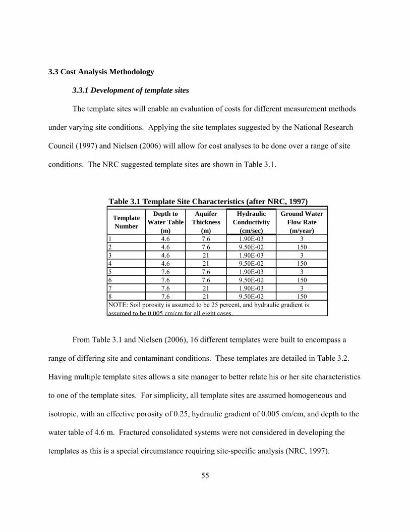
3.3 Cost Analysis Methodology

3.3.1 Development of template sites

The template sites will enable an evaluation of costs for different measurement methods

under varying site conditions. Applying the site templates suggested by the National Research

Council (1997) and Nielsen (2006) will allow for cost analyses to be done over a range of site

conditions. The NRC suggested template sites are shown in Table 3.1.

Table 3.1 Template Site Characteristics (after NRC, 1997)

Template Number

Depth to Water Table

(m)

Aquifer Thickness

(m)

Hydraulic Conductivity

(cm/sec)

Ground Water Flow Rate (m/year)

1 4.6 7.6 1.90E-03 32 4.6 7.6 9.50E-02 1503 4.6 21 1.90E-03 34 4.6 21 9.50E-02 1505 7.6 7.6 1.90E-03 36 7.6 7.6 9.50E-02 1507 7.6 21 1.90E-03 38 7.6 21 9.50E-02 150NOTE: Soil porosity is assumed to be 25 percent, and hydraulic gradient is assumed to be 0.005 cm/cm for all eight cases.

From Table 3.1 and Nielsen (2006), 16 different templates were built to encompass a

range of differing site and contaminant conditions. These templates are detailed in Table 3.2.

Having multiple template sites allows a site manager to better relate his or her site characteristics

to one of the template sites. For simplicity, all template sites are assumed homogeneous and

isotropic, with an effective porosity of 0.25, hydraulic gradient of 0.005 cm/cm, and depth to the

water table of 4.6 m. Fractured consolidated systems were not considered in developing the

templates as this is a special circumstance requiring site-specific analysis (NRC, 1997).

55

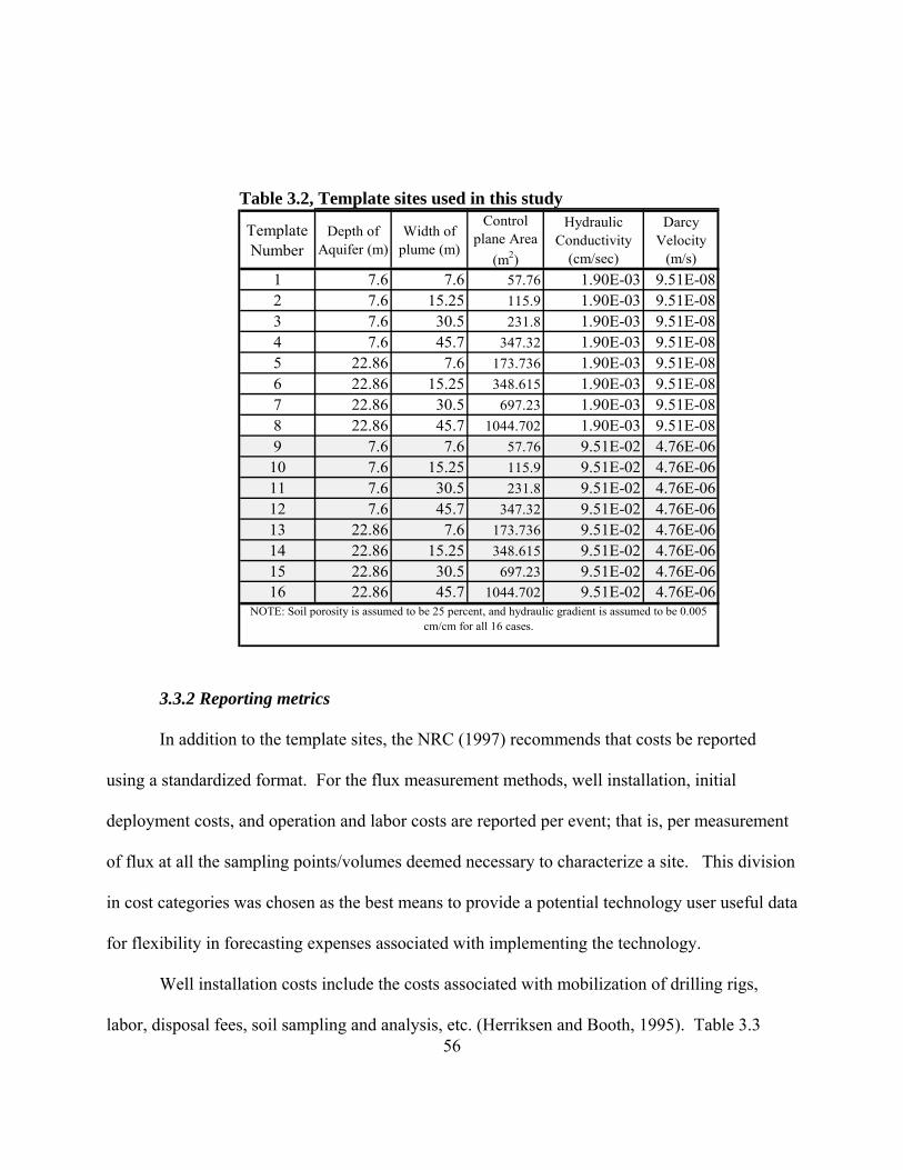
Table 3.2, Template sites used in this study

Template Number

Depth of Aquifer (m)

Width of plume (m)

Control plane Area

(m2)

Hydraulic Conductivity

(cm/sec)

Darcy Velocity

(m/s)1 7.6 7.6 57.76 1.90E-03 9.51E-082 7.6 15.25 115.9 1.90E-03 9.51E-083 7.6 30.5 231.8 1.90E-03 9.51E-084 7.6 45.7 347.32 1.90E-03 9.51E-085 22.86 7.6 173.736 1.90E-03 9.51E-086 22.86 15.25 348.615 1.90E-03 9.51E-087 22.86 30.5 697.23 1.90E-03 9.51E-088 22.86 45.7 1044.702 1.90E-03 9.51E-089 7.6 7.6 57.76 9.51E-02 4.76E-06

10 7.6 15.25 115.9 9.51E-02 4.76E-0611 7.6 30.5 231.8 9.51E-02 4.76E-0612 7.6 45.7 347.32 9.51E-02 4.76E-0613 22.86 7.6 173.736 9.51E-02 4.76E-0614 22.86 15.25 348.615 9.51E-02 4.76E-0615 22.86 30.5 697.23 9.51E-02 4.76E-0616 22.86 45.7 1044.702 9.51E-02 4.76E-06

NOTE: Soil porosity is assumed to be 25 percent, and hydraulic gradient is assumed to be 0.005 cm/cm for all 16 cases.

3.3.2 Reporting metrics

In addition to the template sites, the NRC (1997) recommends that costs be reported

using a standardized format. For the flux measurement methods, well installation, initial

deployment costs, and operation and labor costs are reported per event; that is, per measurement

of flux at all the sampling points/volumes deemed necessary to characterize a site. This division

in cost categories was chosen as the best means to provide a potential technology user useful data

for flexibility in forecasting expenses associated with implementing the technology.

56

Well installation costs include the costs associated with mobilization of drilling rigs,

labor, disposal fees, soil sampling and analysis, etc. (Herriksen and Booth, 1995). Table 3.3

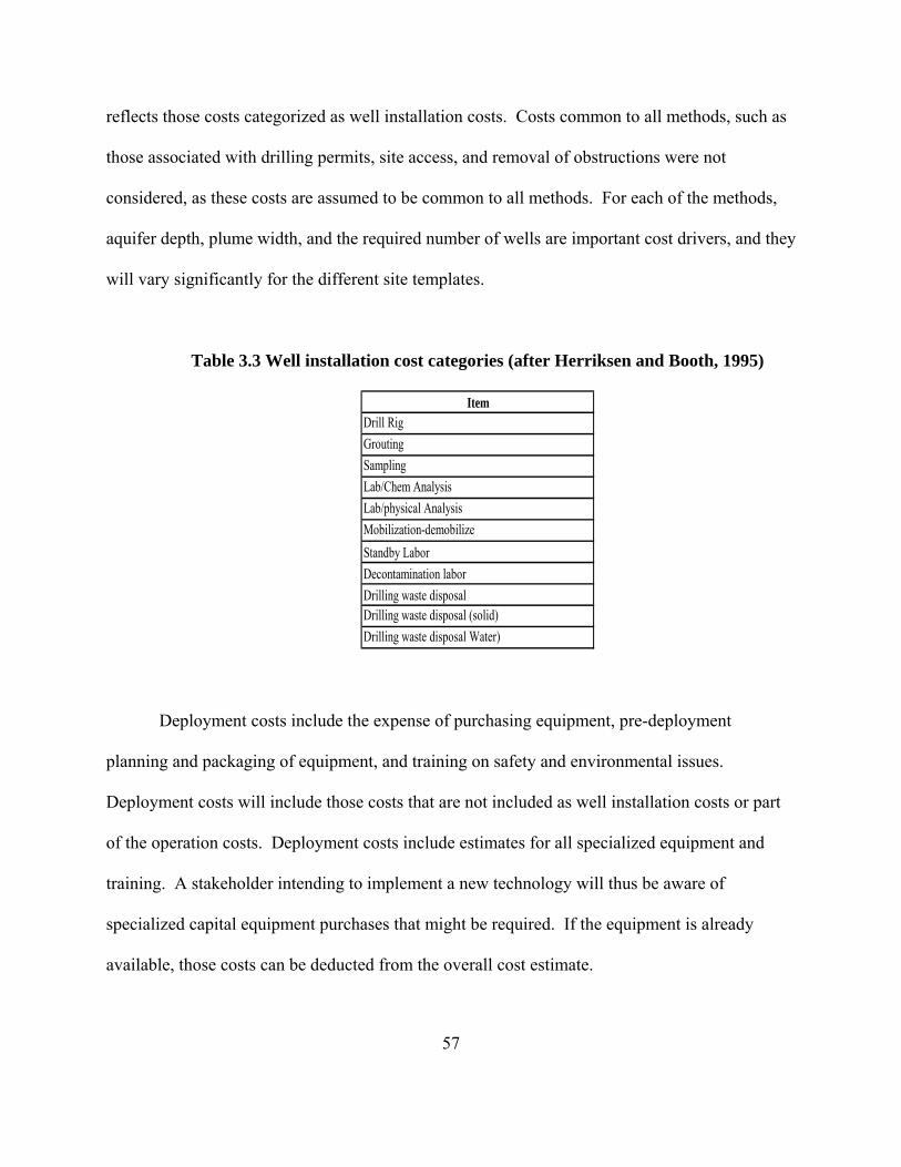
reflects those costs categorized as well installation costs. Costs common to all methods, such as

those associated with drilling permits, site access, and removal of obstructions were not

considered, as these costs are assumed to be common to all methods. For each of the methods,

aquifer depth, plume width, and the required number of wells are important cost drivers, and they

will vary significantly for the different site templates.

Table 3.3 Well installation cost categories (after Herriksen and Booth, 1995)

ItemDrill RigGroutingSamplingLab/Chem AnalysisLab/physical AnalysisMobilization-demobilizeStandby LaborDecontamination laborDrilling waste disposalDrilling waste disposal (solid)Drilling waste disposal Water)

Deployment costs include the expense of purchasing equipment, pre-deployment

planning and packaging of equipment, and training on safety and environmental issues.

Deployment costs will include those costs that are not included as well installation costs or part

of the operation costs. Deployment costs include estimates for all specialized equipment and

training. A stakeholder intending to implement a new technology will thus be aware of

specialized capital equipment purchases that might be required. If the equipment is already

available, those costs can be deducted from the overall cost estimate.

57

58

The operation costs include costs for sample testing, raw materials, waste handling,

consumed supplies, labor for site monitoring, and specific method operation requirements. This

cost will provide a potential technology user an estimate of costs associated with conducting the

method for one test episode. The labor for all monitoring, data analysis, and general site labor is

assumed to be $80 dollars per hour for all labor types. Raw material costs only pertain to the

PFM where the sorbent material is considered a raw material. Not included in operation costs is

electrical power. This cost is highly variable due to such factors as location and hydrogeological

conditions (depth to the water table, hydraulic conductivity). Additionally, in comparison with

other costs, power costs are assumed to be relatively small.

3.3.3 Application of measurement methods to the template sites

The cost to apply a flux measurement method to a particular template site depends on

more than just the site parameters listed in Table 3.2. In particular, the cost of method

application will depend greatly upon site heterogeneity as well as upon the management

objective in making the measurement. For instance, if flux measurements are being made in a

heterogeneous system with the objective of locating source zone “hot spots” (zones of high

contaminant concentration or flux), a very high spatial resolution for sampling will be required.

Conversely, for a homogeneous system, where the goal is to measure overall flux (perhaps to

determine the efficacy of natural attenuation processes in reducing contaminant concentration

and flux), a much lower sampling spatial resolution is needed.

In this study, three levels of spatial resolution, low, medium, and high, will be applied at

the template sites. Note that the impact of spatial resolution on cost will vary, depending on

whether a method is a point method or a volume-averaged method. For point methods, there is a

59

clear relation between resolution and cost. Additionally, point methods can be installed such that

resolution varies both vertically and horizontally. Variations in the resolution of volume-

averaged methods, where pumping wells are installed, are practically limited to the horizontal

direction. Examples of when low, medium, or high resolution sampling will be required are

given below.

1. Low spatial resolution may be used for initial site characterization, or to

characterize a relatively homogeneous aquifer.

2. Medium spatial resolution may be used when evaluating flux in a “typical”

aquifer.

3. High spatial resolution may be appropriate when attempting to locate a source

zone “hot spot” or evaluating the efficacy of a measurement method.

Quantitative definitions of the spatial resolution levels are included in Table 3.4. It was

assumed that research testing of the various methods was conducted at a high spatial resolution.

Therefore, the high spatial resolution values in Table 3.4 were based upon descriptions of those

tests (ESTCP, 2007; USEPA, 2007). The medium and low spatial resolution values were

developed based upon discussions with Wright-Patterson Air Force Base Environmental

Management personnel who oversee multiple contaminated site investigations.

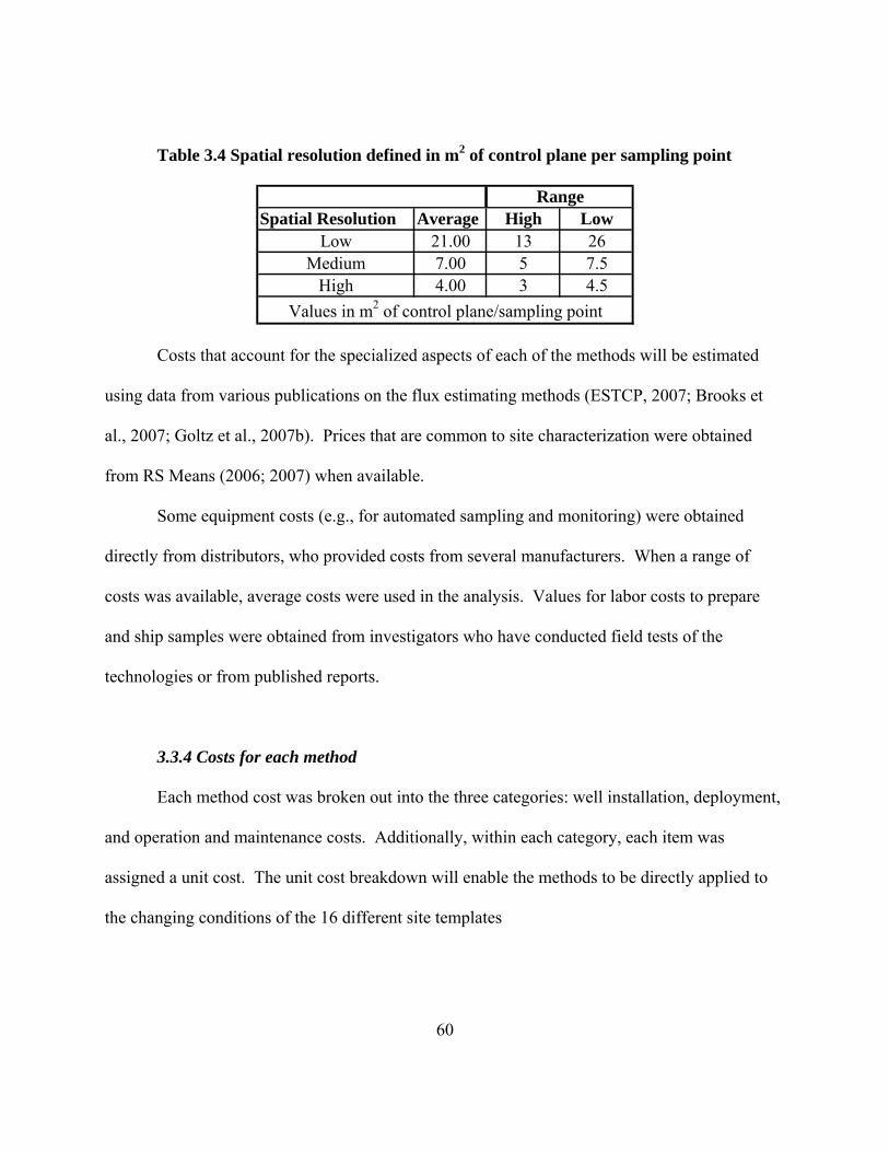
Table 3.4 Spatial resolution defined in m2 of control plane per sampling point

Spatial Resolution Average High LowLow 21.00 13 26

Medium 7.00 5 7.5High 4.00 3 4.5

Range

Values in m2 of control plane/sampling point

Costs that account for the specialized aspects of each of the methods will be estimated

using data from various publications on the flux estimating methods (ESTCP, 2007; Brooks et

al., 2007; Goltz et al., 2007b). Prices that are common to site characterization were obtained

from RS Means (2006; 2007) when available.

Some equipment costs (e.g., for automated sampling and monitoring) were obtained

directly from distributors, who provided costs from several manufacturers. When a range of

costs was available, average costs were used in the analysis. Values for labor costs to prepare

and ship samples were obtained from investigators who have conducted field tests of the

technologies or from published reports.

3.3.4 Costs for each method

Each method cost was broken out into the three categories: well installation, deployment,

and operation and maintenance costs. Additionally, within each category, each item was

assigned a unit cost. The unit cost breakdown will enable the methods to be directly applied to

the changing conditions of the 16 different site templates

60

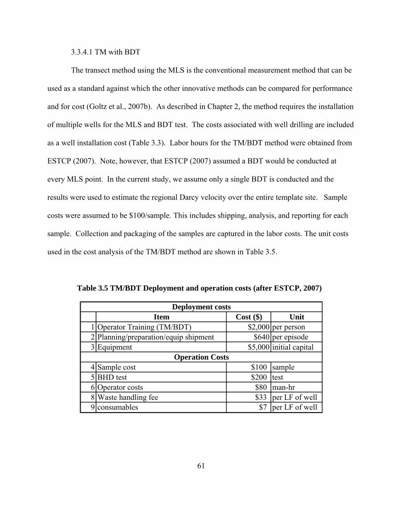
3.3.4.1 TM with BDT

The transect method using the MLS is the conventional measurement method that can be

used as a standard against which the other innovative methods can be compared for performance

and for cost (Goltz et al., 2007b). As described in Chapter 2, the method requires the installation

of multiple wells for the MLS and BDT test. The costs associated with well drilling are included

as a well installation cost (Table 3.3). Labor hours for the TM/BDT method were obtained from

ESTCP (2007). Note, however, that ESTCP (2007) assumed a BDT would be conducted at

every MLS point. In the current study, we assume only a single BDT is conducted and the

results were used to estimate the regional Darcy velocity over the entire template site. Sample

costs were assumed to be $100/sample. This includes shipping, analysis, and reporting for each

sample. Collection and packaging of the samples are captured in the labor costs. The unit costs

used in the cost analysis of the TM/BDT method are shown in Table 3.5.

Table 3.5 TM/BDT Deployment and operation costs (after ESTCP, 2007)

Item Cost ($) Unit1 Operator Training (TM/BDT) $2,000 per person2 Planning/preparation/equip shipment $640 per episode3 Equipment $5,000 initial capital

4 Sample cost $100 sample5 BHD test $200 test6 Operator costs $80 man-hr8 Waste handling fee $33 per LF of well9 consumables $7 per LF of well

Deployment costs

Operation Costs

61

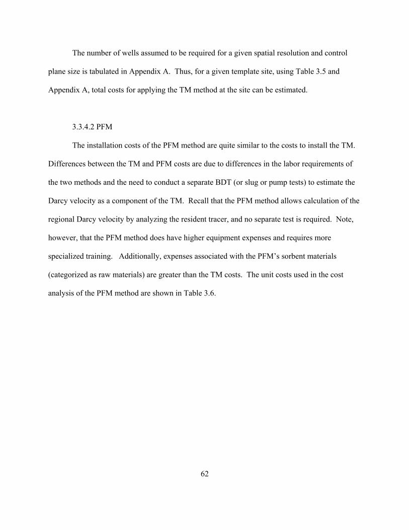
62

The number of wells assumed to be required for a given spatial resolution and control

plane size is tabulated in Appendix A. Thus, for a given template site, using Table 3.5 and

Appendix A, total costs for applying the TM method at the site can be estimated.

3.3.4.2 PFM

The installation costs of the PFM method are quite similar to the costs to install the TM.

Differences between the TM and PFM costs are due to differences in the labor requirements of

the two methods and the need to conduct a separate BDT (or slug or pump tests) to estimate the

Darcy velocity as a component of the TM. Recall that the PFM method allows calculation of the

regional Darcy velocity by analyzing the resident tracer, and no separate test is required. Note,

however, that the PFM method does have higher equipment expenses and requires more

specialized training. Additionally, expenses associated with the PFM’s sorbent materials

(categorized as raw materials) are greater than the TM costs. The unit costs used in the cost

analysis of the PFM method are shown in Table 3.6.

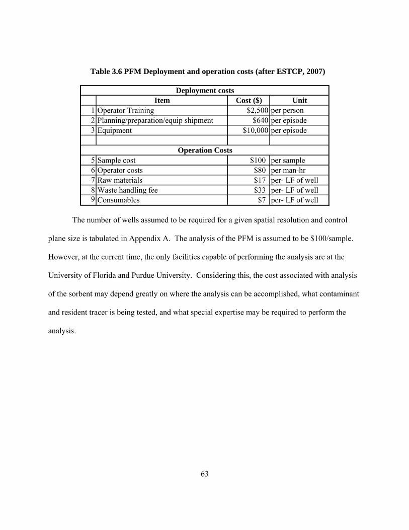
Table 3.6 PFM Deployment and operation costs (after ESTCP, 2007)

Item Cost ($) Unit1 Operator Training $2,500 per person2 Planning/preparation/equip shipment $640 per episode3 Equipment $10,000 per episode

5 Sample cost $100 per sample6 Operator costs $80 per man-hr7 Raw materials $17 per- LF of well8 Waste handling fee $33 per- LF of well9 Consumables $7 per- LF of well

Deployment costs

Operation Costs

The number of wells assumed to be required for a given spatial resolution and control

plane size is tabulated in Appendix A. The analysis of the PFM is assumed to be $100/sample.

However, at the current time, the only facilities capable of performing the analysis are at the

University of Florida and Purdue University. Considering this, the cost associated with analysis

of the sorbent may depend greatly on where the analysis can be accomplished, what contaminant

and resident tracer is being tested, and what special expertise may be required to perform the

analysis.

63

3.3.4.3 MIPT

The unit costs used in the cost analysis of the MIPT method are shown in Table 3.7.

Table 3.7 MIPT Deployment and operation costs

64

3

.6.25.25

Cost ($)

1 $1,0002 $1,2803 $1,5374 $1,1725 $

6 97 18 19 4

10 $20011 $26412 $100 per sample

per lf well

UnitItem

hr /dayhr/well/5xday

per episodeper m3

Sampling analysis-contaminants / tracers

Sample pack/shipConsumables, suppliesWaste handling—contaminated water disposal

Labor-flow monitoringhr/well/5xday

hr/well

Operator Training (MIPT) per personPlanning/preparation/ Equip shipment per episodeEquipment (Automated Monitoring) per well

Tubing per well

Site setup laborLabor-Sampling

Equipment (Pumping/sampling)

Operation Costs

Deployment Costs

An increase in the number of pumping wells will allow for better horizontal (though not

vertical) resolution. In addition, depending on aquifer conductivity, more wells may be needed

to ensure plume capture. Of course, the greater the number of wells, the greater the capital costs

to install the MIPT method. The number of wells assumed to be required for a given spatial

resolution and control plane size is tabulated in Appendix A.

To determine the volume of extracted water, two methods were used. The first method

involves calculating the pump rate and duration required to capture the entire plume width. This

was dependent on the number of wells used, the spacing of the wells, and the hydrologic

properties of the aquifer. Assuming the duration of the test would be five days, pump rates can

be determined from the hydrologic properties specified by the site templates. Results of this

65

method were within 1% of the results calculated using the second method. The second method

determined the volume extracted for a typical MIPT method application; pumping for 24 hours at

each of five predetermined rates. Extracted water disposal costs vary depending on proximity to

a treatment facility, permit requirements if any, and the particular contaminant. For the purpose

of this study, it will be assumed that the cost of contaminated water disposal is $1/gal or

$264/m3. This cost includes the cost for onsite storage, transportation, treatment, and disposal.

The value of $1/gal is a conservative estimate, encompassing costs for treating and disposing of

most non-radioactive materials. USEPA (2008) reports that they will fund up to $0.72/gal for

disposal, but this cost does not take into account the costs for on-site storage.

3.3.4.4 TCW

The TCW method is similar to the MIPT method in that it is a method that obtains a

volume-averaged measurement. The key advantage of the TCW method over the MIPT method

is that the TCW method does not require extraction of contaminated water from the subsurface,

thereby avoiding treatment, transport, and disposal costs. The costs for the TCW in Table 3.8

were largely obtained from a report that included a cost estimate for use of TCWs to treat

contaminated groundwater (AFRL, 1998). The unit costs used in the cost analysis of the TCW

method are shown in Table 3.8.

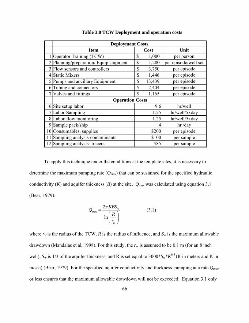
Table 3.8 TCW Deployment and operation costs

Item Cost Unit1 Operator Training (TCW) $ 1,000 per person2 Planning/preparation/ Equip shipment $ 1,280 per episode/well set3 Flow sensors and controllers 3,750$ per episode4 Static Mixers 1,446$ per episode5 Pumps and ancillary Equipment 13,439$ per episode6 Tubing and connectors 2,404$ per episode7 Valves and fittings 1,165$ per episode

6 Site setup labor 9.6 hr/well7 Labor-Sampling 1.25 hr/well/5xday8 Labor-flow monitoring 1.25 hr/well/5xday9 Sample pack/ship 4 hr /day

10 Consumables, supplies $200 per episode11 Sampling analysis-contaminants $100 per sample12 Sampling analysis- tracers $85 per sample

Deployment Costs

Operation Costs

To apply this technique under the conditions at the template sites, it is necessary to

determine the maximum pumping rate (Qmax) that can be sustained for the specified hydraulic

conductivity (K) and aquifer thickness (B) at the site. Qmax was calculated using equation 3.1

(Bear, 1979):

max2

ln

w

w

KBSQRr

π=

⎛ ⎞⎜ ⎟⎝ ⎠

(3.1)

where rw is the radius of the TCW, R is the radius of influence, and Sw is the maximum allowable

drawdown (Mandalas et al, 1998). For this study, the rw is assumed to be 0.1 m (for an 8 inch

well), Sw is 1/3 of the aquifer thickness, and R is set equal to 3000*Sw*K0.5 (R in meters and K in

m/sec) (Bear, 1979). For the specified aquifer conductivity and thickness, pumping at a rate Qmax

or less ensures that the maximum allowable drawdown will not be exceeded. Equation 3.1 only

66

accounts for extraction at the TCW, not injection. Thus, the calculation is conservative, as the

injection serves to minimize drawdown. Equation 3.2 makes use of the Qmax calculated in

equation 3.1 to determine the minimum numbers of well pairs.

max

( )(12N KBi PW f

Q)+

= (3.2)

where N/2 is the number of well pairs for single extraction and injection wells, PW is the capture

zone width, Qmax is the max allowable pump rate, and f is the fraction of recycle between wells.

From the Qmax calculated for the conditions in the different templates, it was determined that only

a single pair of wells is required to meet the template capture zone widths.

To calculate the duration of run time for the TCW test, equation 3.3 is used to calculate

the minimum time for a tracer to move from one TCW to the other (Kim, 2005; Cunningham et

al., 2004):

2

min43

ea HntQ

π= (3.3)

where a, H, ne, and Q represent the half distance between the injection/extraction wells, length of

screened section of wells, aquifer porosity, and the well pumping rates, respectively. To

determine the time required to reach steady-state, tmin will be multiplied by 20. This

approximates the time for the tracers to reach steady-state at the extraction screens (Kim, 2005).

For this study the variables a and H were held to 16.5% of the plume width and 12% of the

aquifer thickness, respectively, across multiple site templates. This is consistent with Kim’s

(2005) experiment design. In addition, the well pumping rate, Q, was held constant at ½Qmax.

67

68

3.4 Decision tree development

We want to develop a decision tree that will serve as a “user-friendly” tool that can be

used to facilitate information transfer to potential technology users. Development of a chart that

requires only initial site investigation data and management objective criteria to determine one or

two preferred flux measurement methods will greatly facilitate the decision making process. The

decision tree will be formatted as a flow chart. With an input of management objectives and

initial site estimates of control plane size, required spatial resolution of the measurements, and

hydraulic conductivity, the decision tree will output the two most economical methods of flux

measurement for application at the site. The user can then chose one of the two most economical

methods based on other subjective factors that have been discussed in this study (e.g., regulatory

acceptability, implementability).

69

IV. Results and Discussion

4.1 Introduction

In section 4.2, we will use data obtained from the literature review on the performance,

advantages, and limitations of the various flux measurement methods to present findings on

performance and ease of implementation. The costs associated with measuring mass flux using

the different methods at the various template sites will be presented in section 4.3. In Section

4.4, we will develop a decision tree and discuss the results obtained from application of the

decision tree methodology.

4.2 Published Data

4.2.1 Performance

To various degrees, all the innovative measurement methods have been tested and

evaluated. From the review in sections 2.3 and 2.4, we may conclude that all the methods have

the potential to effectively measure contaminant mass flux and are viable candidates for

commercial application. Table 4.1 displays comparable information on laboratory and field test

data.

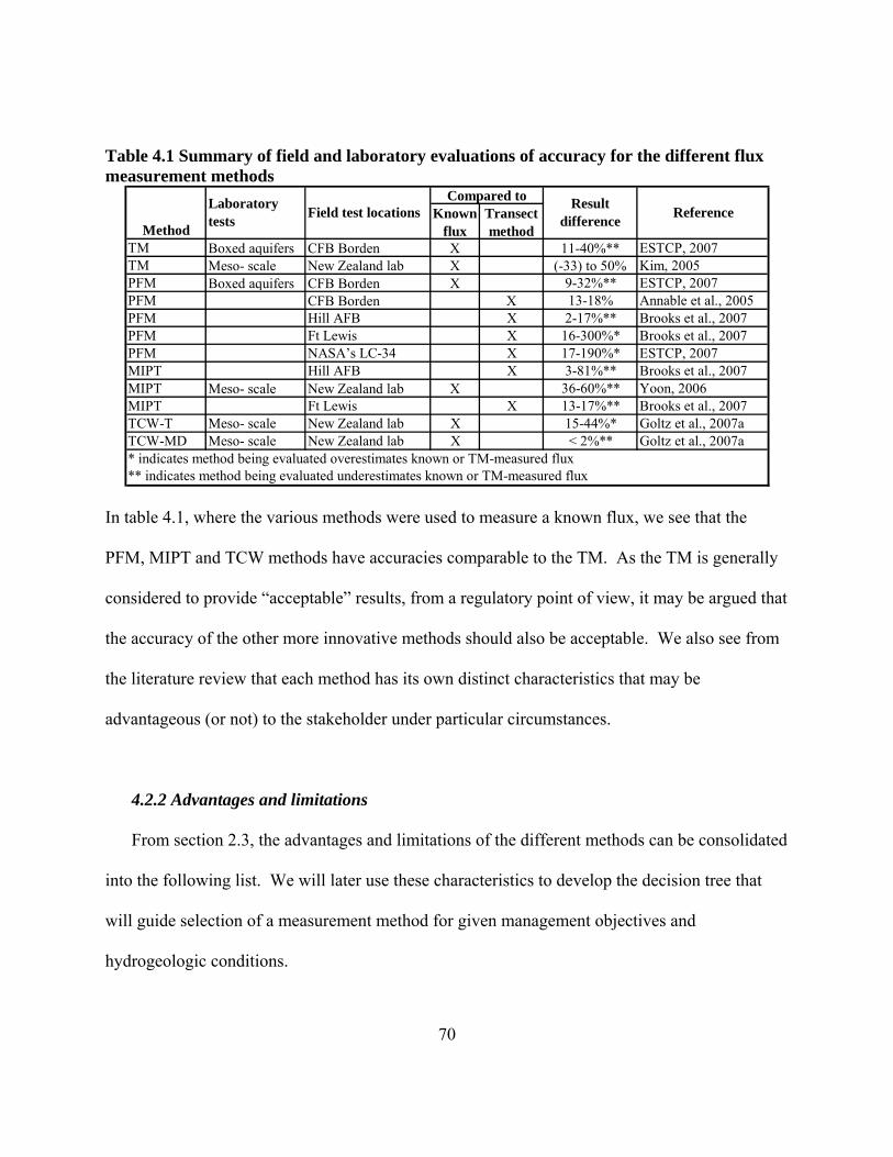
Table 4.1 Summary of field and laboratory evaluations of accuracy for the different flux measurement methods

Known flux

Transect method

TM Boxed aquifers CFB Borden X 11-40%** ESTCP, 2007TM Meso- scale New Zealand lab X (-33) to 50% Kim, 2005PFM Boxed aquifers CFB Borden X 9-32%** ESTCP, 2007PFM CFB Borden X 13-18% Annable et al., 2005PFM Hill AFB X 2-17%** Brooks et al., 2007PFM Ft Lewis X 16-300%* Brooks et al., 2007PFM NASA’s LC-34 X 17-190%* ESTCP, 2007MIPT Hill AFB X 3-81%** Brooks et al., 2007MIPT Meso- scale New Zealand lab X 36-60%** Yoon, 2006MIPT Ft Lewis X 13-17%** Brooks et al., 2007TCW-T Meso- scale New Zealand lab X 15-44%* Goltz et al., 2007aTCW-MD Meso- scale New Zealand lab X < 2%** Goltz et al., 2007a* indicates method being evaluated overestimates known or TM-measured flux ** indicates method being evaluated underestimates known or TM-measured flux

ReferenceMethod

Laboratory tests Field test locations

Compared to Result difference

In table 4.1, where the various methods were used to measure a known flux, we see that the

PFM, MIPT and TCW methods have accuracies comparable to the TM. As the TM is generally

considered to provide “acceptable” results, from a regulatory point of view, it may be argued that

the accuracy of the other more innovative methods should also be acceptable. We also see from

the literature review that each method has its own distinct characteristics that may be

advantageous (or not) to the stakeholder under particular circumstances.

4.2.2 Advantages and limitations

From section 2.3, the advantages and limitations of the different methods can be consolidated

into the following list. We will later use these characteristics to develop the decision tree that

will guide selection of a measurement method for given management objectives and

hydrogeologic conditions.

70

71

Transect Method

• Advantages o Able to provide high resolution definition of contaminant plume in vertical and horizontal

directions o Low costs under homogeneous conditions where high resolution is not required o Ease of use, simplicity of calculations, and short duration o Flexibility--additional wells can be added to locate “hot spots” o Minimal waste disposal

• Limitations o Requires additional tests to estimate flux (BDT to estimate q0 or pump/slug test to

estimate hydraulic conductivity along with piezometer soundings to estimate hydraulic gradient)

o High costs under heterogeneous conditions that require high resolution o Point sampling in time which can’t account for temporal hydrologic changes (e.g. rain

events, seasonal variation) o Potential to miss “hot spots” if sampling resolution is insufficient

Borehole Dilution Test (BDT)

• Advantages o Time-averaged measurement of q0 at a point in space o Low costs under homogeneous conditions where high resolution is not required o The test is of relatively short duration and can be applied under a variety of soil

conditions from unconsolidated to fractured consolidated material • Limitations

o Very sensitive to divergence and convergence factor (α), which is difficult to quantify o In the cases where low permeability and high porosity media are present, diffusion can

dominate and must be accounted for o Requires the use of tracers which may raise some regulatory concerns o Must be done in conjunction with another test (typically the transect method) to measure

concentration

Passive Flux Meter • Advantages

o Time averages both concentration and q0 o Able to provide high resolution definition of contaminant plume in vertical and horizontal

directions o Can also provide the direction of groundwater flow in addition to groundwater flux

magnitude o Doesn’t require electrical power on site, even for deep aquifers; attractive for austere

conditions • Limitations

72

o Very sensitive to divergence and convergence factor (α), which is difficult to quantify o Sensitive to biological activity which can degrade resident tracers (may be especially

problematic if engineered bioremediation is being used as a cleanup remedy) o Requires special knowledge to deploy method and interpret results o Deployment of method requires weeks o Requires the use of tracers which may raise some regulatory concerns

Tandem Circulating Wells • Advantages (Tracer )

o Volume averages both concentration and hydraulic conductivity measurements o Avoids the need to extract and treat contaminated groundwater o Can be conducted for a long time period, allowing for both temporal and spatial

averaging o Can interrogate deep plumes (does not require pumping to surface) o For high hydraulic conductivity systems, small number of wells can interrogate wide

plumes • Limitations (Tracer)

o May require a relatively long and expensive tracer test (days-weeks) o Does not provide the spatial resolution of the point methods, which may be required for

site characterization o Calculations for determining the flux can be rather complex o Has not been field tested o Requires the use of tracers which may raise some regulatory concerns o If contaminant is primarily in the upper or lower region of the aquifer, groundwater

circulation has the potential to spread contamination • Advantages (Multi- dipole)

o Potential for very short test durations o Volume averages both concentration and hydraulic conductivity measurements o Avoids the need to extract and treat contaminated groundwater o Can be conducted for a long time period, allowing for both temporal and spatial

averaging o Can interrogate deep plumes (does not require pumping to surface) o For high hydraulic conductivity systems, small number of wells can interrogate wide

plumes • Limitations (Multi-dipole)

o Small head differences may be difficult to measure o Does not provide the spatial resolution of the point methods, which may be required for

site characterization o If contaminant is primarily in the upper or lower region of the aquifer, circulation pattern

has the potential to spread the contamination

73

Modified Integral Pump Test

• Advantages o Volume averages concentration and q0 measurements o Variable pumping rates allow flexibility in accommodating seasonal flow events as the

wells within the transect can be pumped at varying rates to accommodate changing conditions

o Flexible in that additional wells can be placed without incurring large costs o Duration of test is relatively short (about a week) o Easy calculations

• Limitations o Extracts groundwater and therefore requires the treatment of contaminated water o May be difficult to measure small head differences o Does not provide the spatial resolution of the point methods, which may be required for

site characterization, although emplacement of additional wells will allow for increased resolution horizontally

4.3 Cost Comparison

4.3.1 Cost versus size of control plane

Holding the hydraulic conductivity, depth of aquifer, and spatial resolution constant, a

cost versus transect width plot shows how cost increases with increasing control plane width

(Figure 4.1). This analysis was conducted for all three spatial resolutions (low, medium, and

high). In addition, the analysis was conducted for different aquifer thicknesses. As would be

expected, costs generally increased with an increase in the width of the control plane or aquifer

thickness.

Cost increased for the point methods as width increased, as these methods require more

wells and sampling points for a given spatial resolution (Figure 4.1). This is not surprising, as

we assume that to obtain the same spatial resolution, these two point methods require the same

number of wells and the same number of samples. However, there are cost differences between

the two methods, though these differences lead to similar cost increases as transect width

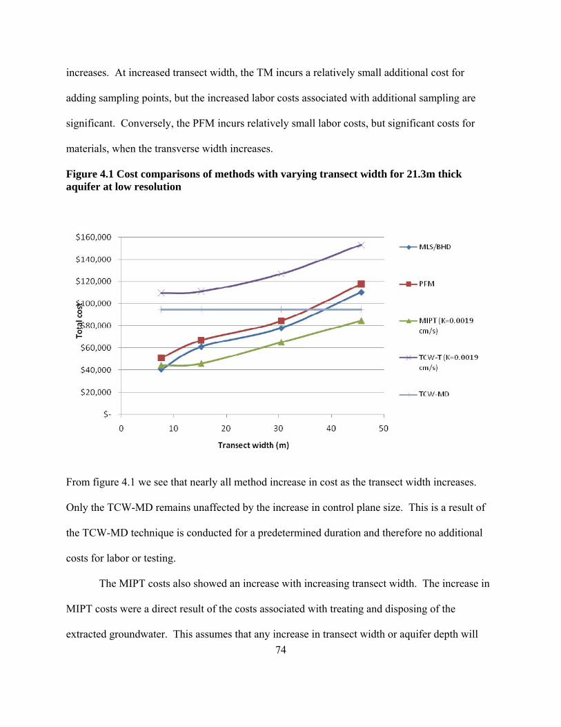
increases. At increased transect width, the TM incurs a relatively small additional cost for

adding sampling points, but the increased labor costs associated with additional sampling are

significant. Conversely, the PFM incurs relatively small labor costs, but significant costs for

materials, when the transverse width increases.

Figure 4.1 Cost comparisons of methods with varying transect width for 21.3m thick aquifer at low resolution

From figure 4.1 we see that nearly all method increase in cost as the transect width increases.

Only the TCW-MD remains unaffected by the increase in control plane size. This is a result of

the TCW-MD technique is conducted for a predetermined duration and therefore no additional

costs for labor or testing.

The MIPT costs also showed an increase with increasing transect width. The increase in

MIPT costs were a direct result of the costs associated with treating and disposing of the

extracted groundwater. This assumes that any increase in transect width or aquifer depth will 74

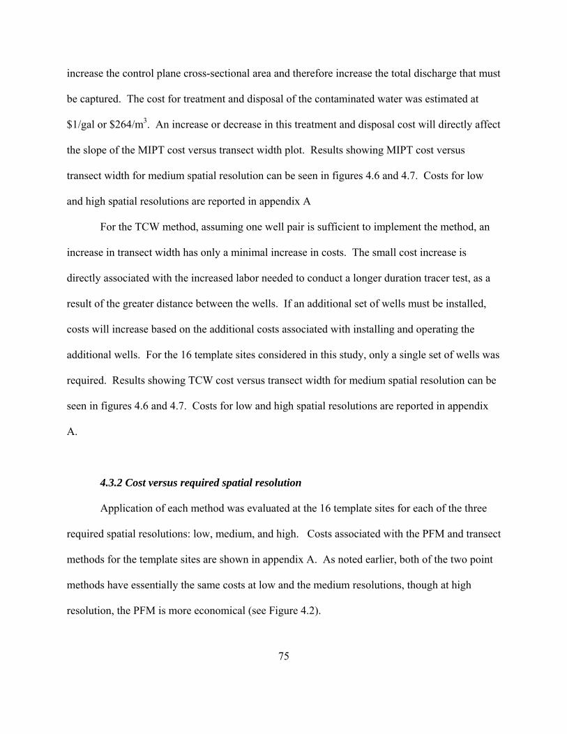
75

increase the control plane cross-sectional area and therefore increase the total discharge that must

be captured. The cost for treatment and disposal of the contaminated water was estimated at

$1/gal or $264/m3. An increase or decrease in this treatment and disposal cost will directly affect

the slope of the MIPT cost versus transect width plot. Results showing MIPT cost versus

transect width for medium spatial resolution can be seen in figures 4.6 and 4.7. Costs for low

and high spatial resolutions are reported in appendix A

For the TCW method, assuming one well pair is sufficient to implement the method, an

increase in transect width has only a minimal increase in costs. The small cost increase is

directly associated with the increased labor needed to conduct a longer duration tracer test, as a

result of the greater distance between the wells. If an additional set of wells must be installed,

costs will increase based on the additional costs associated with installing and operating the

additional wells. For the 16 template sites considered in this study, only a single set of wells was

required. Results showing TCW cost versus transect width for medium spatial resolution can be

seen in figures 4.6 and 4.7. Costs for low and high spatial resolutions are reported in appendix

A.

4.3.2 Cost versus required spatial resolution

Application of each method was evaluated at the 16 template sites for each of the three

required spatial resolutions: low, medium, and high. Costs associated with the PFM and transect

methods for the template sites are shown in appendix A. As noted earlier, both of the two point

methods have essentially the same costs at low and the medium resolutions, though at high

resolution, the PFM is more economical (see Figure 4.2).

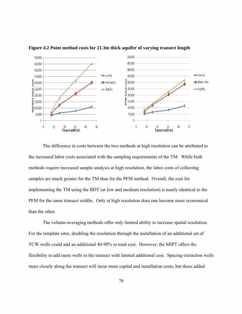
Figure 4.2 Point method costs for 21.3m thick aquifer of varying transect length

The difference in costs between the two methods at high resolution can be attributed to

the increased labor costs associated with the sampling requirements of the TM. While both

methods require increased sample analysis at high resolution, the labor costs of collecting

samples are much greater for the TM than for the PFM method. Overall, the cost for

implementing the TM using the BDT (at low and medium resolution) is nearly identical to the

PFM for the same transect widths. Only at high resolution does one become more economical

than the other.

The volume-averaging methods offer only limited ability to increase spatial resolution.

For the template sites, doubling the resolution through the installation of an additional set of

TCW wells could add an additional 40-90% to total cost. However, the MIPT offers the

flexibility to add more wells to the transect with limited additional cost. Spacing extraction wells

more closely along the transect will incur more capital and installation costs, but these added

76

costs will be reduced by cost savings in disposal. The more pumps along the transect, the less

volume of water needs to be extracted to capture the plume. The reduction in disposal cost for

the 16 different site templates for the addition of a single well ranged from 5-10% with

efficiency effects decreasing with increase of total number of wells. The addition of more wells

along the transect will permit greater horizontal resolution. Vertical spatial resolution would not

be increased for fully screened wells, such as are used in the MIPT method. Figure 4.3 shows

the influence on cost of adding wells to a control plane for the MIPT.

Figure 4.3 Effect of additional MIPT wells on cost of treating and disposing extracted water (a) K = 0.002 cm/s and (b) K = 0.095 cm/s (note different y-axis scales) a b

Where well installation to depths of 12 and 26 meters is roughly $4,000 and $9,000 per

well, respectively, it seems from Figure 4.3 that only at higher hydraulic conductivities and

larger control plane areas is the costs savings obtained by lower water treatment and disposal

costs great enough to compensate for the cost of installing additional wells. At lower hydraulic

77

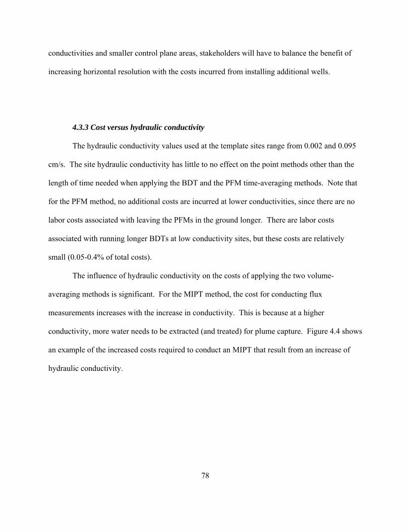
78

conductivities and smaller control plane areas, stakeholders will have to balance the benefit of

increasing horizontal resolution with the costs incurred from installing additional wells.

4.3.3 Cost versus hydraulic conductivity

The hydraulic conductivity values used at the template sites range from 0.002 and 0.095

cm/s. The site hydraulic conductivity has little to no effect on the point methods other than the

length of time needed when applying the BDT and the PFM time-averaging methods. Note that

for the PFM method, no additional costs are incurred at lower conductivities, since there are no

labor costs associated with leaving the PFMs in the ground longer. There are labor costs

associated with running longer BDTs at low conductivity sites, but these costs are relatively

small (0.05-0.4% of total costs).

The influence of hydraulic conductivity on the costs of applying the two volume-

averaging methods is significant. For the MIPT method, the cost for conducting flux

measurements increases with the increase in conductivity. This is because at a higher

conductivity, more water needs to be extracted (and treated) for plume capture. Figure 4.4 shows

an example of the increased costs required to conduct an MIPT that result from an increase of

hydraulic conductivity.

Figure 4.4 Total cost for measuring contaminant flux for a 21.3m thick aquifer at different values of hydraulic conductivity

Interestingly, TCW tracer technique costs decrease with increasing conductivity. This is

because a significant fraction of the cost of implementing the TCW method is the labor and

analytical costs associated with conducting the tracer test. The increase in conductivity will

result in a shorter tracer test (see Equations 3.1 and 3.2). With labor at $80/hour and duration

ranging from days to weeks, the cost savings for the TCW tracer technique at a high conductivity

site can be considerable. For the TCW multi-dipole technique, cost will generally not change

with changing hydraulic conductivity. However, high hydraulic conductivity will result in

smaller head differences which may produce inaccuracies. Figure 4.5 compares costs of

applying the TCW tracer technique at high and low conductivity sites for two aquifer

thicknesses.

79

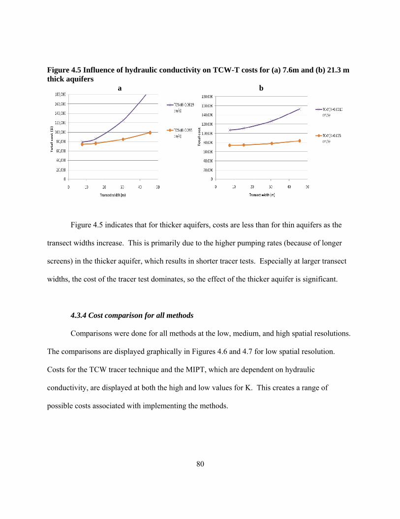
Figure 4.5 Influence of hydraulic conductivity on TCW-T costs for (a) 7.6m and (b) 21.3 m thick aquifers a b

Figure 4.5 indicates that for thicker aquifers, costs are less than for thin aquifers as the

transect widths increase. This is primarily due to the higher pumping rates (because of longer

screens) in the thicker aquifer, which results in shorter tracer tests. Especially at larger transect

widths, the cost of the tracer test dominates, so the effect of the thicker aquifer is significant.

4.3.4 Cost comparison for all methods

Comparisons were done for all methods at the low, medium, and high spatial resolutions.

The comparisons are displayed graphically in Figures 4.6 and 4.7 for low spatial resolution.

Costs for the TCW tracer technique and the MIPT, which are dependent on hydraulic

conductivity, are displayed at both the high and low values for K. This creates a range of

possible costs associated with implementing the methods.

80

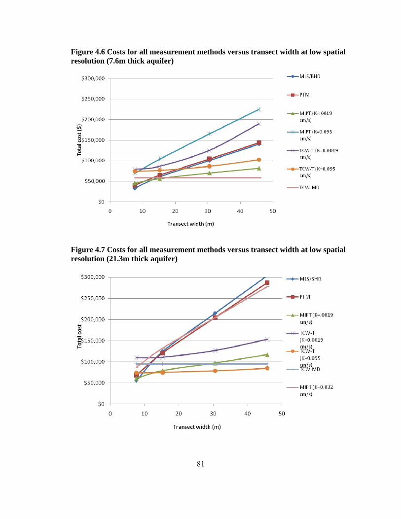
Figure 4.6 Costs for all measurement methods versus transect width at low spatial resolution (7.6m thick aquifer)

Figure 4.7 Costs for all measurement methods versus transect width at low spatial resolution (21.3m thick aquifer)

81

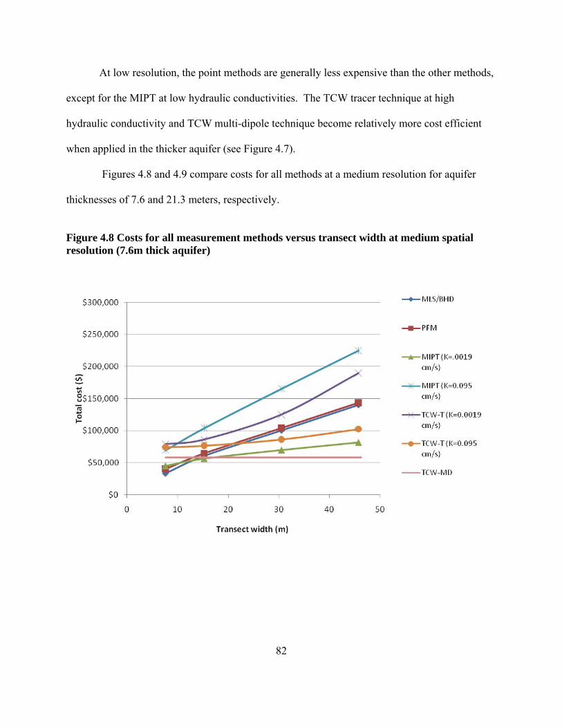
At low resolution, the point methods are generally less expensive than the other methods,

except for the MIPT at low hydraulic conductivities. The TCW tracer technique at high

hydraulic conductivity and TCW multi-dipole technique become relatively more cost efficient

when applied in the thicker aquifer (see Figure 4.7).

Figures 4.8 and 4.9 compare costs for all methods at a medium resolution for aquifer

thicknesses of 7.6 and 21.3 meters, respectively.

Figure 4.8 Costs for all measurement methods versus transect width at medium spatial resolution (7.6m thick aquifer)

82

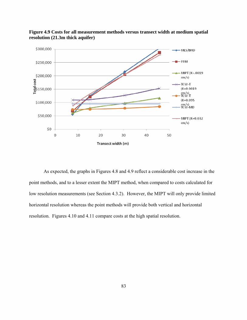
Figure 4.9 Costs for all measurement methods versus transect width at medium spatial resolution (21.3m thick aquifer)

As expected, the graphs in Figures 4.8 and 4.9 reflect a considerable cost increase in the

point methods, and to a lesser extent the MIPT method, when compared to costs calculated for

low resolution measurements (see Section 4.3.2). However, the MIPT will only provide limited

horizontal resolution whereas the point methods will provide both vertical and horizontal

resolution. Figures 4.10 and 4.11 compare costs at the high spatial resolution.

83

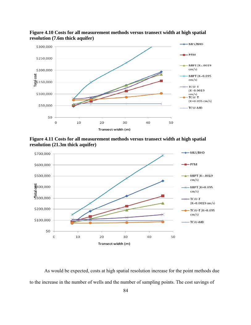
Figure 4.10 Costs for all measurement methods versus transect width at high spatial resolution (7.6m thick aquifer)

Figure 4.11 Costs for all measurement methods versus transect width at high spatial resolution (21.3m thick aquifer)

As would be expected, costs at high spatial resolution increase for the point methods due

to the increase in the number of wells and the number of sampling points. The cost savings of

84

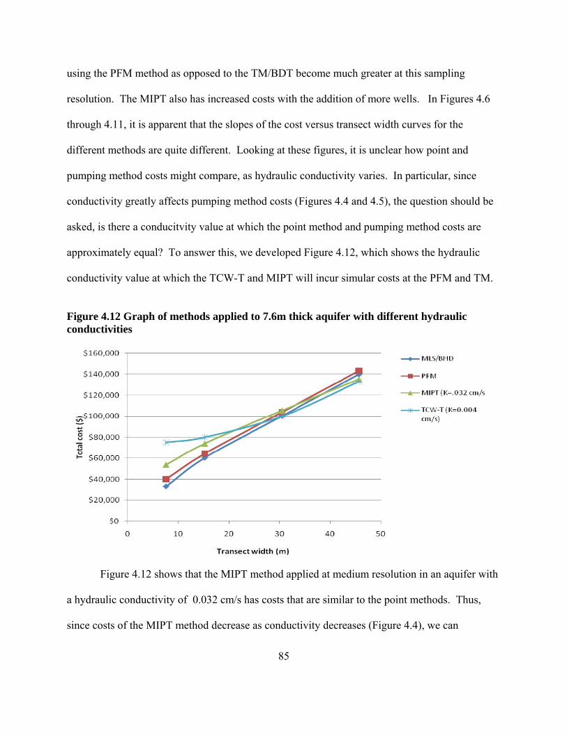
using the PFM method as opposed to the TM/BDT become much greater at this sampling

resolution. The MIPT also has increased costs with the addition of more wells. In Figures 4.6

through 4.11, it is apparent that the slopes of the cost versus transect width curves for the

different methods are quite different. Looking at these figures, it is unclear how point and

pumping method costs might compare, as hydraulic conductivity varies. In particular, since

conductivity greatly affects pumping method costs (Figures 4.4 and 4.5), the question should be

asked, is there a conducitvity value at which the point method and pumping method costs are

approximately equal? To answer this, we developed Figure 4.12, which shows the hydraulic

conductivity value at which the TCW-T and MIPT will incur simular costs at the PFM and TM.

Figure 4.12 Graph of methods applied to 7.6m thick aquifer with different hydraulic conductivities

Figure 4.12 shows that the MIPT method applied at medium resolution in an aquifer with

a hydraulic conductivity of 0.032 cm/s has costs that are similar to the point methods. Thus,

since costs of the MIPT method decrease as conductivity decreases (Figure 4.4), we can

85

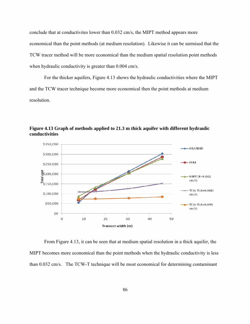
conclude that at conductivites lower than 0.032 cm/s, the MIPT method appears more

economical than the point methods (at medium resolution). Likewise it can be surmised that the

TCW tracer method will be more economical than the medium spatial resolution point methods

when hydraulic conductivity is greater than 0.004 cm/s.

For the thicker aquifers, Figure 4.13 shows the hydraulic conductivities where the MIPT

and the TCW tracer technique become more economical then the point methods at medium

resolution.

Figure 4.13 Graph of methods applied to 21.3 m thick aquifer with different hydraulic conductivities

From Figure 4.13, it can be seen that at medium spatial resolution in a thick aquifer, the

MIPT becomes more economical than the point methods when the hydraulic conductivity is less

than 0.032 cm/s. The TCW-T technique will be most economical for determining contaminant

86

87

mass flux at the full range of hydraulic conductivities. This is true for both the MIPT and the

TCW methods for the two aquifer thicknesses used in the template sites.

Having reviewed the factors that influence cost, we now develop a decision tree that can

be used by site managers to help them incorporate all factors relevant to the question of which

flux measurement technology to use at a site, with given management objectives and site

conditions.

4.4 Decision Tree

The decision tree is built with the assumption that basic information on site conditions

and management objectives is available (see figure 4.14). Initial investigation of the site should

provide the stakeholder with estimates of hydraulic conductivity, aquifer thickness and

contaminant plume width, hydraulic gradient, and mean flow direction. From these estimates, a

series of decision points will guide the stakeholder to the appropriate and most cost effective

approach to measuring contaminant mass flux.

The decision tree, in figure 4.14, is limited to the range of the variables used in the 16

template sites (e.g., hydraulic conductivities between 0.0019 and 0.095cm/s) and the assumptions

made in Chapter 3 (e.g., the cost for treating extracted groundwater is $1/gal).

Referring to section 1.2, the objective of the flux measurement may be to either: (1)

assess risk in order to develop cleanup priorities or evaluate remediation effectiveness or (2)

characterize the site to design a remediation technology. The management objective will drive

the required spatial resolution. For assessing risk or evaluating remediation methods, high

spatial resolution will typically not be required; however, high resolution may be necessary for

site characterization to support a remedial design.

88

In addition to the objective of the measurement, a second factor that affects the required

measurement resolution is the heterogeneity of the site and contaminant distribution. Another

factor that affects the decision is the scope of the measurement, as quantified by the control plane

area. The control plane area is calculated as the product of the plume width and the aquifer

saturated thickness. The control planes at the template sites range in area from 60m2 to nearly

1,000m2. Based on this range, we have chosen 300m2 as a convenient point to delineate large

and small control planes.

The last factor used in the decision tree is hydraulic conductivity. The hydraulic

conductivities at the template sites range from 0.002 to 0.095 cm/s. Based on this range, we

have chosen 0.032 cm/s as a convenient point to delineate low and high conductivities. Note that

this also happens to be the conductivity at which the MIPT becomes more economical than the

PFM and transect method.

The decision tree outputs the two most cost-effective measurement methods for the given

management objectives, spatial resolution, control plane size, and hydraulic conductivity. With

these two suggested methods in mind, the technology user must then consider additional factors

to ensure the method that is ultimately selected satisfies other requirements. These other factors

include regulatory considerations, whether or not the technology is readily available, and

complexity of method application and analysis.

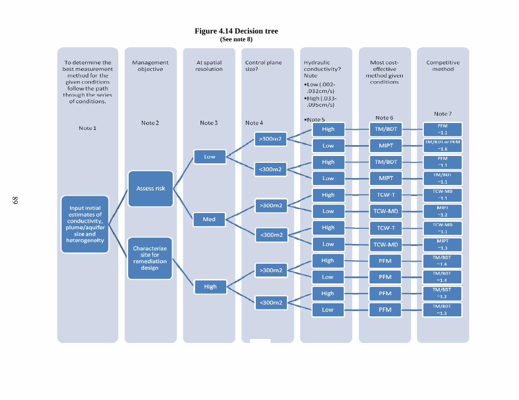
89

Figure 4.14 Decision tree (See note 8)

89

91

4.4.1 Notes for decision tree

This decision tree is a qualitative method of accounting for site conditions and

management objectives to help a technology user decide on what flux measurement

technology might be most suitable. If site conditions are well known and the required

spatial resolution defined, the cost comparison figures (Figures 4.6 through 4.13) might

be more useful in selecting the most cost-effective technology.

1. Preliminary site investigations should provide estimates of hydraulic conductivity,

aquifer depth, hydraulic gradient, plume size, and heterogeneity.

2. Management objects should provide direction on the type of mass flux

investigation to be conducted. Site characterization to support a remedial design,

particularly in support of a source zone cleanup, may require considerable spatial

detail while a risk assessment in a relatively homogeneous aquifer could be

accomplished with low resolution sampling.

3. Spatial resolution is driven by the management objective and level of

heterogeneity. Detail on the definition of low, medium, and high spatial

resolution can be found in Section 3.3.3.

4. For this decision tree to apply, the size of the control plane should be between 60

and 1000 m2. 300 m2 was chosen as the dividing area between large and small

control planes. This point is large enough to encompass both aquifer depth

templates yet small enough to allow for the illustrate advantages of the point

90

91

methods for small areas. This is also the point in which cost differences tend to

become more defined under the templates. For control plane areas that are about

300m2, both paths (large and small options) should be considered and potential

technologies confirmed using the cost comparison figures (Figures 4.6 through

4.13).

5. This decision tree only applies to hydraulic conductivities ranging from 0.002 to

0.095 cm/s. Hydraulic conductivity is separated into high and low ranges,

delineated by a value of 0.032 cm/s. This value was selected because it is also the

value below which the MIPT method becomes competitive with the point

methods. For hydraulic conductivities near 0.032 cm/s, both paths (high and low)

should be considered and potential technologies confirmed using the cost

comparison figures (Figures 4.6 through 4.13).

6. The end product are the two least expensive methods.

7. The second “competitive method” is provided with a relative cost increase. For

example, the annotation TCW-T, ~1.1 next to TM/BDT indicates that the TCW

tracer method is estimated to be 1.1 times as expensive as the TM method under

the specified conditions.

8. In addition to the criteria in the decision tree, the potential user should review

other subjective factors provided in Table 4.2 to ensure the method will meet

requirements and avoid possible regulatory or implementation problems.

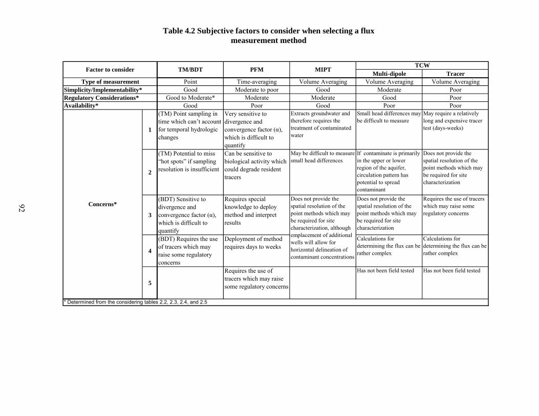
Table 4.2 Subjective factors to consider when selecting a flux measurement method

Multi-dipole TracerPoint Time-averaging Volume Averaging Volume Averaging Volume AveragingGood Moderate to poor Good Moderate Poor

Good to Moderate* Moderate Moderate Good PoorGood Poor Good Poor Poor

1

(TM) Point sampling in time which can’t account for temporal hydrologic changes

Very sensitive to divergence and convergence factor (α), which is difficult to quantify

Extracts groundwater and therefore requires the treatment of contaminated water

Small head differences may be difficult to measure

May require a relatively long and expensive tracer test (days-weeks)

2

(TM) Potential to miss “hot spots” if sampling resolution is insufficient

Can be sensitive to biological activity which could degrade resident tracers

May be difficult to measure small head differences

If contaminate is primarily in the upper or lower region of the aquifer, circulation pattern has potential to spread contaminant

Does not provide the spatial resolution of the point methods which may be required for site characterization

3

(BDT) Sensitive to divergence and convergence factor (α), which is difficult to quantify

Requires special knowledge to deploy method and interpret results

Does not provide the spatial resolution of the point methods which may be required for site characterization

Requires the use of tracers which may raise some regulatory concerns

4

(BDT) Requires the use of tracers which may raise some regulatory concerns

Deployment of method requires days to weeks

Calculations for determining the flux can be rather complex

Calculations for determining the flux can be rather complex

5

Requires the use of tracers which may raise some regulatory concerns

Has not been field tested Has not been field tested

TCW

Simplicity/Implementability*

Concerns*Does not provide the spatial resolution of the point methods which may be required for site characterization, although emplacement of additional wells will allow for horizontal delineation of contaminant concentrations

* Determined from the considering tables 2.2, 2.3, 2.4, and 2.5

Type of measurement

Regulatory Considerations*Availability*

Factor to consider TM/BDT PFM MIPT

92

92 91

4.4.2 Examples for decision tree use

Example 1:

• Aquifer thickness of 10 m

• Plume width of 40 m

• Hydraulic conductivity of 0.07 cm/s

• Low resolution required to assess risk (homogeneous conditions)

Given these conditions, the decision tree shows the TM with the BDT is the least

expensive method followed by the PFM, which is 10% more expensive. This can be seen

in figure 4.6 where the cost for implementing the TM is about $50K and the PFM about

$55K. From table 4.2, we see there are potential regulatory concerns with the use of the

BDT. In addition, at low resolution, the TM could possibly miss “hot spots” if the

contaminant distribution and aquifer are not homogeneous. If this is the case, it may be

necessary to use a higher sampling resolution or employ a pump method.

Example 2




• Medium resolution required to assess risk (homogeneous aquifer, different source

locations)

93

Using the decision tree for the given conditions, the TCW-MD is the least costly method

followed by the MIPT. Referencing table 4.2 there are no issues that would impact a

decision to employ either method.

Example 3




• High resolution required (site investigation for designing a remediation)

Using the decision tree, the optimum economic choice is the PFM with the next option

being the TM with an estimated cost of 40% over the cost of the PFM. Reviewing table

4.2, assistance and training may be required to design, assemble and deploy the PFM.

However the savings associated with using the PFM make the PFM more attractive.

When using the PFM, inaccuracies in estimating the convergence/divergence factor

should be considered.

94

V. Conclusions

5.1 Summary

This study examined methods for measuring contaminant mass flux in

groundwater. Mass flux measurements may be used to 1) prioritize contaminated

groundwater sites for remediation, 2) evaluate the effectiveness of source removal

technologies or natural attenuation processes, and 3) define a source term for

groundwater contaminant transport modeling, which can be used as a tool to achieve the

previous two objectives.

The following mass flux measurement methods, some in use and some emerging,

were discussed in detail: (1) the conventional transect method using multi-level sampling

(MLS), (2) the borehole dilution test (BDT) which complements the MLS by measuring

groundwater flux, (3) the modified integral pump test (MIPT), (4) passive flux meters

(PFMs), and (5) tandem circulating wells (TCWs). Discussion included the advantages

and limitations of each method, as well as the results of field and laboratory evaluations

on method accuracy.

Detailed cost analyses were conducted to quantify the relative costs of applying

the different measurement methods. In accordance with recommendations that have been

made to facilitate technology transfer, the costs of applying each method to 16 different

template sites, which spanned a broad spectrum of hydrogeological conditions, were

determined. The costs were then compared to determine which method was most

economical under which site condition. Finally, the results of the literature review and

95

the cost analysis provided the necessary information to develop a decision tree to aid

potential technology users in determining which method would best meet both

management objectives and economic constraints.

5.2 Conclusions

The results of the cost analysis offer insight as to how various factors, which are a

function of site conditions and management objectives, affect the costs for implementing

the different methods. Each variable affects the cost of methods differently. The results

of the analysis, which looks at the impact of these factors on cost, follows.

5.2.1 Spatial resolution

Spatial resolution has the greatest effect on the cost of the two point methods: the

TM and PFM methods. As the spatial resolution increases, so do the costs of applying

the methods. We found that at high resolution, the PFM will be less costly than the

TM/BDT method. The volume averaging MIPT and TCW methods do not offer the

same spatial resolution flexibility or capability as the point methods. The MIPT can

provide limited horizontal resolution without incurring large cost increases. The cost for

adding an additional well is tempered by a reduction in extracted groundwater treatment

costs as a result of more efficient pumping to meet the capture width. The TCW only

offers increased resolution by installing additional well pairs. This would increase costs

by 40 to 90% for only a limited increase in horizontal resolution.

96

5.2.2 Control plane area

The area of the control plane is driven by the plume width and the aquifer

thickness and both measurements have an influence on the costs of implementing the

methods. An increase in control plane area increases costs for the point methods, as more

sampling points and wells are required to maintain a specified level of sampling

resolution. Application of the MIPT will also become more costly as the control plane

area increases. This is because more water flows across the control plane, resulting in the

need for more contaminated groundwater to be captured and extracted, and therefore

treated and disposed of. In this study, the TCW method only used a single pair of wells.

Thus, the only additional TCW-T method costs associated with an increase in control

plane area are due to increases in tracer test time (thereby incurring additional labor and

analytical costs) as a result of having to locate the TCWs farther apart from each other.

The TCW multi-dipole method would not incur any additional costs.

5.2.3 Hydraulic conductivity

The hydraulic conductivity has little influence on the cost of the point methods.

The only effect that lower conductivity would have on the point methods is that the

duration of the PFM and BDT methods would increase. The MIPT and TCW method

costs are sensitive to changes in hydraulic conductivity. The MIPT, when treatment of

extracted groundwater is required, will sustain higher costs as conductivity increases.

Conversely, the TCW tracer technique will incur higher costs as conductivity decreases,

due to increases in the tracer test duration. Assuming additional TCWs are not required,

97

the cost of applying the TCW multi-dipole technique is not affected by conductivity

though method accuracy may be improved at low conductivities, due to larger head

differences to measure at the wells. Hydraulic conductivity can be a decisive element

when choosing between methods.

5.2.3 Conclusion on method costs

Field and laboratory test results of the newer methods indicate that their accuracy

is as good as, or better than, the accuracy of the TM, the currently accepted method.

Comparing test results with known fluxes and to that of the TM, under the same

conditions, provide the “apple to apples” comparison suited for stakeholder decision

making.

Based on the cost analysis, it can be concluded that for low spatial resolution the

point methods will be the least expensive. This is true for control plane sizes smaller

than 300 m2 and where the hydraulic conductivity is greater than 0.016 cm/s. If the

hydraulic conductivity is less than 0.016 cm/s, it is likely that the MIPT will be most cost

effective for larger control planes. Additionally, for control plane areas approaching or

exceeding 1,000 m2, the TCW-MD technique will provide the most economical means to

measure flux.

At a medium sampling resolution, cost comparisons of the methods illustrate how

the pumping methods can either exceed or be under the costs associated with the point

methods. At control plane areas lower than about 30 m2, the point methods prove least

expensive. It is also apparent that at low hydraulic conductivities, the MIPT will be least

98

expensive for a wide range of control plane sizes (200 to 600m2). At larger control

planes and low hydraulic conductivity, the TCW-MD will be the least expensive.

At high sampling resolutions, the pumping methods are necessarily excluded.

Aside from very small control planes (less than 70 m2), the PFM will prove to be less

costly than the TM. This difference increases as the size of the control plane increases.

5.3 Recommendations for future research

1. Define spatial resolution as a function of measurement objective and

heterogeneity (of both the aquifer and the contaminant) more rationally. This

study based the relationship (in Table 3.4) upon anecdotal reports of past

practices. Hopefully, a measure of heterogeneity (perhaps correlation length), in

concert with a specified measurement objective, can be used to obtain a

quantitative measure of spatial resolution.

2. Develop software to automate the decision tree. Produce a user-friendly interface

where initial site investigation parameters and management objectives are input

and the most applicable and economic measurement methods are output.

3. In the current study, we try to provide decision makers with credible cost

and performance information in order to facilitate transfer and commercialization

of an innovative measurement technology. How successful was this approach? Is

the information presented in a useable form? What else do potential measurement

technology users need to facilitate technology transfer?

99

References

AFRL, IRP, Aerobic cometabolic in situ bioremediation technology guidance manual and screening software user’s guide, Earth Tech, INC Alexandria VA., 1998

Annable MD, Hatfield K, Cho J, et al. Field-scale evaluation of the passive flux meter for

simultaneous measurement of groundwater and contaminant fluxes. Environmental Science & Technology, 39(18), 7194-7201. 2005.

API, Groundwater Remediation Strategies Tool. Regulatory Analysis and Scientific

Affairs Department, Publication No. 4730, American Petroleum Institute, Washington DC. 2003.

Arnon, S., Z. Ronen, E. Adar, A. Yakirevich, and R. Nativ. Two-dimensional distribution

of microbial activity and flow patterns within naturally fractured chalk. Journal of Contaminant Hydrology 79, no. 3–4: 165–186. 2005

Basu, N. B., Rao, P. S. C., Poyer, I. C., Annable, M. D., & Hatfield, K. Flux-based

assessment at a manufacturing site contaminated with trichloroethylene. Journal of Contaminant Hydrology, 86(1-2), 105-127. 2006.

Bauer, S., Bayer-Raich, M., Holder, T., Kolesar, C., Muller, D., and Ptak, T.,

Quantification of groundwater contamination in an urban area using integral pump tests. Journal of Contaminant Hydrology, 75(3-4), 183-213. 2004.

Bernstein, A., Adar., Yakirevich A., and Nativ R. Dilution Tests in a Low-Permeability

Fractured Aquifer: Matrix Diffusion Effect, Ground Water 45, no. 2: 235–241. 2007.

Bidaux, P., and Tsang, C.F., Fluid flow patterns around a well bore or an underground

drift with complex skin effects: Water Resources Research, v. 27, no. 11, p. 2,993–3,008. 1991.

Bockelmann, A., T. Ptak, and G. Teutsch, An analytical quantification of mass fluxes and

natural attenuation rate constants at a former gasworks site, Journal of Contaminant Hydrology, 53: 429-453, 2001.

Bockelmann, A., D. Zamfirescu, T. Ptak, P. Grathwohl, and G. Teutsch, Quantification of

mass fluxes and natural attenuation rates at an industrial site with a limited monitoring network: a case study, Journal of Contaminant Hydrology, 60: 97-121, 2003.

100

Brooks, M.C., Wood, A.L., Annable, M.D., Hatfield, K., Cho, J., Holbert, C., Rao,

P.S.C., Enfield, C.G., Lynch, K and Smith, R.E. Changes in Contaminant Mass Discharge from DNAPL Source Mass Depletion: Evaluation at two field sites, Journal of Contaminant Hydrology, In Review, Submitted September 2007.

Brooks M.C., A.L. Wood, US Environmental Protection Agency, Ground Water and

Ecosystems Restoration Research, Ada, Ok. Personal correspondence. 2008 Campbell, T. J., K. Hatfield, H. Klammler, M. D. Annable, and P.S.C. Rao. Magnitude

and directional measures of water and Cr(VI) fluxes by passive flux meter. Environmental Science and Technology, 40, 6392-6397. 2006.

Drost, W., Klotz, D., Koch, A., Moser, H., Neumaier, F., Rauert, W., Point dilution

methods of investigating groundwater flow by means of isotopes. Water Resources Research, 4 (1), 125– 146. 1968.

Einarson, M. D. and D. M. Mackay, Predicting impacts of groundwater contamination,

Environmental Science and Technology, 35(3):66A-73A, 2001. ESTCP Project CU-0114, 2006a University of Florida and Purdue University, Field

Demonstration and Validation of a New Device for Measuring Water and Solute Fluxes at CFB Borden, November 2006.

ESTCP Project CU-0114, 2006b University of Florida and Purdue University, Field

Demonstration and Validation of a New Device for Measuring Water and Solute Fluxes, December 2007.

Fetter C. W., Applied Hydrogeology. Prentice Hall Inc., Simon and Schuster, New

Jersey. 1994 Goltz, M. N., J. Huang, M. E. Close, M. Flintoft, and L. Pang, Use of horizontal flow

treatment wells to measure hydraulic conductivity without groundwater extraction, submitted Journal of Contaminant Hydrology, 2004.

Goltz M. N., J. Huang, M. E. Close, M. J. Flintoft, and L. Pang, Use of Tandem Wells To

Measure Hydraulic Conductivity, submitted Journal of Contaminant Hydrology, 2007a.

Goltz M. N., S. Kim, H. Yoon and J. Park, Review of Groundwater Contaminant Mass

Flux Measurement, Korean Society of Environmental Engineers, 2007b.

101

Guilbeault, M. A., B. L. Parker, and J. A. Cherry, Mass and flux distributions from DNAPL zones in sandy aquifers, Ground Water, 43(1): 70-86, 2005.

Groundwater foundation. (2008, March 10). The Groundwater Foundation. Retrieved

September 15, 2007, from The Groundwater Foundation: http://www.groundwater.org/gi/sourcesofgwcontam.html. 2008

Halevy, E., Moser, H., Zellhofer, O., and Zuber.A. Borehole dilution techniques: a critical review. Proceedings of the 1966 Symposium of the International Atomic Energy Agency, 531-564. 1967

Hatfield, K., Annable, M., Cho, J., Rao, P. S. C., & Klammler, H. A direct passive

method for measuring water and contaminant fluxes in porous media. Journal of Contaminant Hydrology, 75(3), 155-181. 2004.

Huang, J., M. E. Close, L. Pang, and M. N. Goltz, Innovative method to measure flux of

dissolved contaminants in groundwater, Fourth International Conference on Remediation of Chlorinated and Recalcitrant Compounds, Monterey California, 24-27 May 2004.

Huang, J., Goltz, M. N., & Roberts, P. V. Comment on ‘Analytical solution for solute

transport resulting from instantaneous injection in streams with transient storage’ by F. de smedt, W. brevis, and P. debels, 2005. Journal of Hydrology, 330(3-4), 759-760. 2006

Kabala, Z. J., Dipole flow test; a new single-borehole test for aquifer characterization,

Water Resource Research, 29(1): 99-107, 1993. Kao, C.M., Wang, Y.S. Field investigation of natural attenuation and intrinsic

biodegradation rates at an underground storage tank site. Environ. Geol., 40 (4–5), 622– 631. 2001.

Kim, S. J., Validation of an innovative groundwater contaminant flux measurement method,

MS thesis, AFIT/GES/ENV/05-02, Department of system and engineering management, Air Force Institute of Technology, Wright-Patterson AFB OH, 2005.

Klammler, H., Hatfield, K., and Annable, M. D. Concepts for measuring horizontal

groundwater flow directions using the passive flux meter. Advances in Water Resources, 30(4), 984-997, 2007.

Kubert M., and M. Finkel, Contaminant mass discharge estimation in groundwater based

on multi-level point measurements: A numerical evaluation of expected errors. Journal of Contaminant Hydrology, 2005.

102

Lee, J., Rao, P. S. C., Poyer, I. C., Toole, R. M., Annable, M. D., & Hatfield, K. Oxyanion flux characterization using passive flux meters: Development and field testing of surfactant-modified granular activated carbon. Journal of Contaminant Hydrology, 92(3-4), 208-229, 2007.

Lile O.B., M Morris, J.S. Ronning. Estimating groundwater flow velocity from changes

in contact resistance during a saltwater tracer experiment. Journal of Applied Geophysics, 38(2), 105-114, 1997.

Mandalas, G. C., Christ, J. A., & Goltz, M. N. Screening software for an innovative in

situ bioremediation technology. Bioremediation Journal, 2(1), 7-15, 1998. McCarty, P. L., M. N. Goltz, G. D. Hopkins, M. E. Dolan, J. P. Allan, B. T. Kawakami,

and T. J. Carrothers, Full-scale evaluation of in situ cometabolic Degradation of trichloroethylene in groundwater through toluene injection, Environmental Science and Technology, 32(1):88-100, 1998.

Meinardus, H. W., Dwarakanath, V., Ewing, J., Hirasaki, G. J., Jackson, R. E., Jin, M., et

al. Performance assessment of NAPL remediation in heterogeneous alluvium. Journal of Contaminant Hydrology, 54(3-4), 173-193. 2002.

National Research Council (NRC), Innovations in ground water and soil cleanup.

Washington DC. 1997. Nielsen David M., Practical Handbook of Environmental Site Characterization and

Ground-Water Monitoring, CRC press, 2006. Pitrak, M. (Department of Applied Geophysics, Charles University), Mares, S., & Kobr,

M. A simple borehole dilution technique in measuring horizontal ground water flow. Ground Water, 45(1), 89-92. 2007.

Ptak, T., L. Alberti, S. Bauer, M. Bayer-Raich, S. Ceccon, P. Elsass, T. Holder,

C.Kolesar, D. Muller, C. Padovani, G. Rinck, G. Schafer, M. Tanda, G. Teutsch, and A. Zanini, Integrated concept for groundwater remediation, Integral groundwater investigation, 2003.

Rao, P. S. C., Annable, M.D., Sillan, R.K., Dai, D., Hatfield, K., Graham, W.D., Wood,

A.L., Enfield, C.G., Field-scale evaluation of in situ cosolvent flushing for enhanced aquifer remediation, Water Resources Research, 33 (12), 2673-2686. 1997.

RS Means, Environmental remediation estimating methods. Construction publishers and

consultants, Kingston MA. 2003

103

RS Means, Heavy construction cost data, Construction publishers and consultants, Kingston MA. 2006

Wilson J. T., W. A. Mandell, F.L. Paillet, E.R. Bayless, and R.T. Hanson et al. An

evaluation of borehole flowmeters used to measure horizontal ground-water flow in limestones of Indiana, Kentucky, and Tennessee, 1999, Water-Resources Investigations Report 01-413. 2001.

SERDP. Annual Technical Report: Impacts of DNAPL source zone treatment:

Experimental and modeling assessment of the benefits of partial source removal, December, 2004.

Teutsch, G., Ptak, T., Schwarz, R. and Holder, T. (2000): A new integral procedure for

quantification of contaminant mass flow in groundwater. Ground Water 4(5), 170-175. 2000

Yoon, H. Validation of methods to measure mass flux of a groundwater contaminant ,

MS thesis, AFIT/GES/ENV/06-02, Department of system and engineering management, Air Force Institute of Technology, Wright-Patterson AFB OH, 2006.

NGWA. (n.d). National Groundwater Association. Retrieved Feb 7, 2008, from

Groundwater facts: http://www.ngwa.org/public/gw_use/faqs.aspx, 2008. USEPA, Ground Water and Ecosystems Restoration Division, Flux-Based Methods for

DNAPL Remediation Design and Assessment 2007 Draft USEPA. (2008, January 10). United States Environmental Protection Agency. Retrieved

08 08, 2007, from Under ground storage tanks: http://www.epa.gov/oust/cat/index.htm, 2008.

USGAO. Leaking Underground Storage Tanks. Washington, D.C. 20548: Government

Accountability Office. 2007.

104

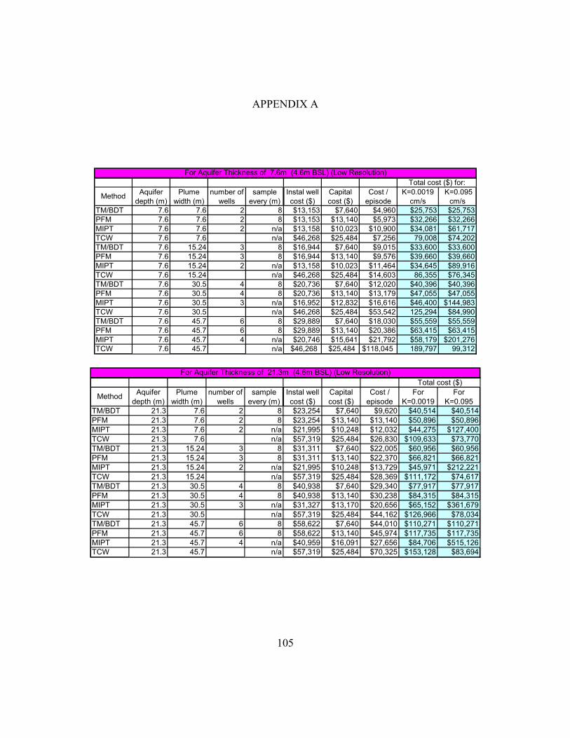
APPENDIX A

TM/BDT 7.6 7.6 2 8 $13,153 $7,640 $4,960 $25,753 $25,753PFM 7.6 7.6 2 8 $13,153 $13,140 $5,973 $32,266 $32,266MIPT 7.6 7.6 2 n/a $13,158 $10,023 $10,900 $34,081 $61,717TCW 7.6 7.6 n/a $46,268 $25,484 $7,256 79,008 $74,202TM/BDT 7.6 15.24 3 8 $16,944 $7,640 $9,015 $33,600 $33,600PFM 7.6 15.24 3 8 $16,944 $13,140 $9,576 $39,660 $39,660MIPT 7.6 15.24 2 n/a $13,158 $10,023 $11,464 $34,645 $89,916TCW 7.6 15.24 n/a $46,268 $25,484 $14,603 86,355 $76,345TM/BDT 7.6 30.5 4 8 $20,736 $7,640 $12,020 $40,396 $40,396PFM 7.6 30.5 4 8 $20,736 $13,140 $13,179 $47,055 $47,055MIPT 7.6 30.5 3 n/a $16,952 $12,832 $16,616 $46,400 $144,983TCW 7.6 30.5 n/a $46,268 $25,484 $53,542 125,294 $84,990TM/BDT 7.6 45.7 6 8 $29,889 $7,640 $18,030 $55,559 $55,559PFM 7.6 45.7 6 8 $29,889 $13,140 $20,386 $63,415 $63,415MIPT 7.6 45.7 4 n/a $20,746 $15,641 $21,792 $58,179 $201,276TCW 7.6 45.7 n/a $46,268 $25,484 $118,045 189,797 99,312

K=0.0019 cm/s

K=0.095 cm/s

For Aquifer Thickness of 7.6m (4.6m BSL) (Low Resolution)Total cost ($) for:

Method Aquifer depth (m)

Plume width (m)

number of wells

sample every (m)

Instal well cost ($)

Capital cost ($)

Cost / episode

TM/BDT 21.3 7.6 2 8 $23,254 $7,640 $9,620 $40,514 $40,514PFM 21.3 7.6 2 8 $23,254 $13,140 $13,140 $50,896 $50,896MIPT 21.3 7.6 2 n/a $21,995 $10,248 $12,032 $44,275 $127,400TCW 21.3 7.6 n/a $57,319 $25,484 $26,830 $109,633 $73,770TM/BDT 21.3 15.24 3 8 $31,311 $7,640 $22,005 $60,956 $60,956PFM 21.3 15.24 3 8 $31,311 $13,140 $22,370 $66,821 $66,821MIPT 21.3 15.24 2 n/a $21,995 $10,248 $13,729 $45,971 $212,221TCW 21.3 15.24 n/a $57,319 $25,484 $28,369 $111,172 $74,617TM/BDT 21.3 30.5 4 8 $40,938 $7,640 $29,340 $77,917 $77,917PFM 21.3 30.5 4 8 $40,938 $13,140 $30,238 $84,315 $84,315MIPT 21.3 30.5 3 n/a $31,327 $13,170 $20,656 $65,152 $361,679TCW 21.3 30.5 n/a $57,319 $25,484 $44,162 $126,966 $78,034TM/BDT 21.3 45.7 6 8 $58,622 $7,640 $44,010 $110,271 $110,271PFM 21.3 45.7 6 8 $58,622 $13,140 $45,974 $117,735 $117,735MIPT 21.3 45.7 4 n/a $40,959 $16,091 $27,656 $84,706 $515,126TCW 21.3 45.7 n/a $57,319 $25,484 $70,325 $153,128 $83,694

For K=0.0019

For K=0.095

For Aquifer Thickness of 21.3m (4.6m BSL) (Low Resolution)Total cost ($)


Plume width (m)

number of wells

sample every (m)


Capital cost ($)

Cost / episode

105

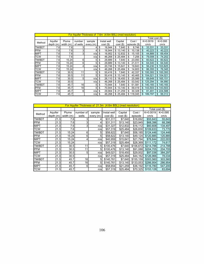
TM/BDT 7.6 7.6 3 4 16,944$ 7,640$ 8,746$ 33,331$ 33,331$ PFM 7.6 7.6 3 4 16,944$ 13,140$ 10,138$ 40,223$ 40,223$ MIPT 7.6 7.6 3 n/a 16,952$ 12,832$ 15,105$ 44,889$ 69,454$ TCW 7.6 7.6 n/a 46,268$ 25,484$ 7,256$ 79,008$ 74,202$ TM/BDT 7.6 15.24 6 5 29,889$ 7,640$ 23,093$ 60,622$ 60,622$ PFM 7.6 15.24 6 5 29,889$ 13,140$ 21,511$ 64,540$ 64,540$ MIPT 7.6 15.24 4 n/a 20,746$ 15,641$ 19,843$ 56,230$ 103,825$ TCW 7.6 15.24 n/a 46,268$ 25,484$ 14,603$ 86,355$ 76,345$ TM/BDT 7.6 30.5 11 5 50,416$ 7,640$ 42,337$ 100,393$ 100,393$ PFM 7.6 30.5 11 5 50,416$ 13,140$ 40,465$ 104,021$ 104,021$ MIPT 7.6 30.5 5 n/a 26,110$ 18,450$ 25,089$ 69,649$ 165,151$ TCW 7.6 30.5 n/a 46,268$ 25,484$ 53,542$ 125,294$ 84,990$ TM/BDT 7.6 45.7 16 5 70,944$ 7,640$ 61,581$ 140,165$ 140,165$ PFM 7.6 45.7 16 5 70,944$ 13,140$ 59,419$ 143,503$ 143,503$ MIPT 7.6 45.7 6 n/a 29,904$ 21,259$ 30,328$ 81,491$ 224,588$ TCW 7.6 45.7 n/a 46,268$ 25,484$ 118,045$ 189,797$ 99,312$

K=0.0019 cm/s

K=0.095 cm/s

For Aquifer Thickness of 7.6m (4.6m BSL) (med resolution)Total cost ($)


Plume width (m)

number of wells

sample every (m)


Capital cost ($)

Cost / episode ($)

TM/BDT 21.3 7.6 3 4 $31,311 $7,640 $16,692 $55,643 55,643PFM 21.3 7.6 3 4 $31,311 $13,140 $23,945 $68,396 68,396MIPT 21.3 7.6 3 n/a $31,327 $12,832 $16,112 $60,608 134,497TCW 21.3 7.6 n/a $57,319 $25,484 $26,830 $109,633 73,770TM/BDT 21.3 15.24 6 5 $58,622 $7,640 $58,185 $124,446 124,446PFM 21.3 15.24 6 5 $58,622 $13,140 $49,124 $120,885 120,885MIPT 21.3 15.24 4 n/a $40,959 $15,641 $21,794 $78,844 222,003TCW 21.3 15.24 n/a $57,319 $25,484 $28,369 $111,172 74,617TM/BDT 21.3 30.5 11 5 $100,476 $7,640 $106,672 $214,788 214,788PFM 21.3 30.5 11 5 $100,476 $13,140 $91,088 $204,705 204,705MIPT 21.3 30.5 5 n/a $49,021 $18,450 $29,002 $97,036 384,297TCW 21.3 30.5 n/a $57,319 $25,484 $44,162 $126,966 78,034TM/BDT 21.3 45.7 16 5 $140,761 $7,640 $155,159 $303,560 303,560PFM 21.3 45.7 16 5 $140,761 $13,140 $133,053 $286,954 286,954MIPT 21.3 45.7 6 n/a $58,654 $21,259 $36,192 $116,780 547,200TCW 21.3 45.7 n/a $57,319 $25,484 $70,325 $153,128 83,694

K=0.0019 cm/s

K=0.095 cm/s

For Aquifer Thickness of 21.3m (4.6m BSL) (med resolution)Total cost ($)


Plume width (m)

number of wells

sample every (m)


Capital cost ($)

Cost / episode

106

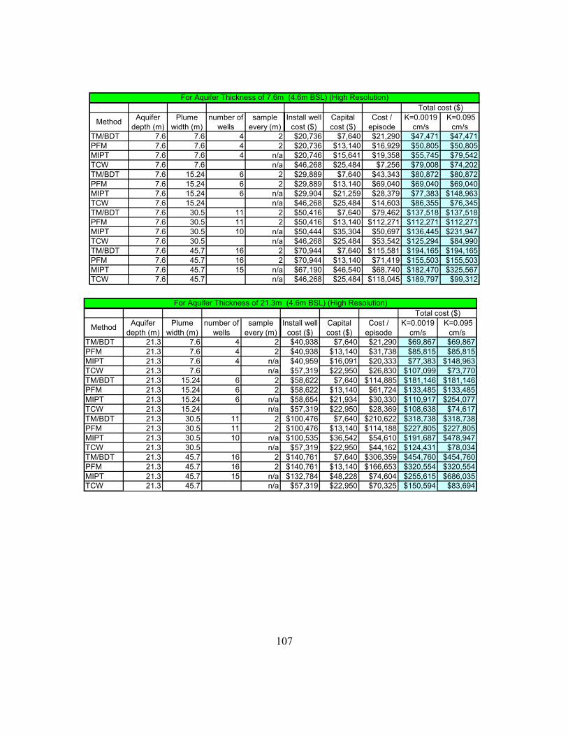
107


K=0.0019 cm/s

K=0.095 cm/s

For Aquifer Thickness of 7.6m (4.6m BSL) (High Resolution)Total cost ($)


Plume width (m)

number of wells

sample every (m)

Install well cost ($)

Capital cost ($)

Cost / episode


K=0.0019 cm/s

K=0.095 cm/s

For Aquifer Thickness of 21.3m (4.6m BSL) (High Resolution)Total cost ($)


Plume width (m)

number of wells

sample every (m)

Install well cost ($)

Capital cost ($)

Cost / episode

REPORT DOCUMENTATION PAGE Form Approved OMB No. 074-0188

The public reporting burden for this collection of information is estimated to average 1 hour per response, including the time for reviewing instructions, searching existing data sources, gathering and maintaining the data needed, and completing and reviewing the collection of information. Send comments regarding this burden estimate or any other aspect of the collection of information, including suggestions for reducing this burden to Department of Defense, Washington Headquarters Services, Directorate for Information Operations and Reports (0704-0188), 1215 Jefferson Davis Highway, Suite 1204, Arlington, VA 22202-4302. Respondents should be aware that notwithstanding any other provision of law, no person shall be subject to an penalty for failing to comply with a collection of information if it does not display a currently valid OMB control number. PLEASE DO NOT RETURN YOUR FORM TO THE ABOVE ADDRESS. 1. REPORT DATE (DD-MM-YYYY)

27-03-2008

2. REPORT TYPE Master’s Thesis

3. DATES COVERED (From – To) August 2007 – March 2008

5a. CONTRACT NUMBER 5b. GRANT NUMBER

4. TITLE AND SUBTITLE An Evaluation and Implementation Guide for Current Groundwater Mass Flux Measurement Practices

5c. PROGRAM ELEMENT NUMBER

5d. PROJECT NUMBER

5e. TASK NUMBER

6. AUTHOR(S) Wheeldon, Jack G., Major, USAF

5f. WORK UNIT NUMBER

7. PERFORMING ORGANIZATION NAMES(S) AND ADDRESS(S) Air Force Institute of Technology Graduate School of Engineering and Management (AFIT/EN) 2950 Hobson Way, Building 640 WPAFB OH 45433-8865

8. PERFORMING ORGANIZATION REPORT NUMBER AFIT/GEM/ENV/08-M23

10. SPONSOR/MONITOR’S ACRONYM(S) U.S. EPA, NRMRL, GWERD

9. SPONSORING/MONITORING AGENCY NAME(S) AND ADDRESS(ES) U.S. Environmental Protection Agency Ground Water and Ecosystem Restoration Division (GWERD) National Risk Management Research Laboratory 919 Kerr Research Drive, P.O. Box 1198 Ada, OK 74821

11. SPONSOR/MONITOR’S REPORT NUMBER(S)

12. DISTRIBUTION/AVAILABILITY STATEMENT APPROVED FOR PUBLIC RELEASE; DISTRIBUTION UNLIMITED.

13. SUPPLEMENTARY NOTES 14. ABSTRACT

Contaminant mass flux is an important parameter needed for decision making at sites with contaminated groundwater. New and potentially better methods for measuring mass flux are emerging. This study looks at the conventional transect method (TM), and the newer passive flux meter (PFM), modified integral pump test (MIPT), and tandem circulating well (TCW) methods. In order to facilitate transfer and application of these innovative technologies, it is essential that potential technology users have access to credible information that addresses technology capabilities, limitations, and costs. This study provides such information on each of the methods by reviewing implementation practices and comparing the costs of applying the methods at 16 standardized “template” sites. The results of the analysis are consolidated into a decision tree that can be used to determine which measurement method would be most effective, from cost and performance standpoints, in meeting management objectives at a given site.

The study found that, in general: (1) the point methods (i.e. the TM and PFM) were less expensive to use to characterize smaller areas of contamination while the pumping methods (the MIPT and TCW) would be more economical for larger areas, (2) the pumping methods are not capable of high resolution sampling, which may be required to characterize heterogeneous systems or to design remediations, and (3) when high resolution is required, the PFM is more economical then the TM. Finally, the study demonstrated that, arguably, test results of the newer methods indicate that their accuracy is as good as, or better than, the accuracy of the TM, the currently accepted method. 15. SUBJECT TERMS Groundwater mass flux evaluation, Implementation guide and decision analysis 16. SECURITY CLASSIFICATION OF:

19a. NAME OF RESPONSIBLE PERSON Goltz, Mark N., USAF

a. REPORT

U

b. ABSTRACT

U

c. THIS PAGE

U

17. LIMITATION OF ABSTRACT

UU

18. NUMBER OF PAGES

121

19b. TELEPHONE NUMBER (Include area code) (937) 255-3636, ext 4638 ([email protected])

Standard Form 298 (Rev. 8-98) Prescribed by ANSI Std. Z39-18

an evaluation of current mass flux measurement practices ... · mipt and tcw) would be more ... 4.2...

Documents