an estimation of the aggregate wheat supply function for
TRANSCRIPT

i
An estimation of the aggregate wheat supply function for
Zimbabwe
M.Sc. Thesis
Knowledge Gweru
February 2019

ii
An estimation of the aggregate wheat supply function for
Zimbabwe
Knowledge Gweru
February 2019
M.Sc. Thesis
Agricultural Economics and Rural Policy Group
Wageningen University
Supervisor: dr. J.H.M. (Jack) Peerlings

iii
Table of Contents Abstract ....................................................................................................................................... i
Acknowledgements .................................................................................................................... ii
Abbreviations ............................................................................................................................ iii
Chapter 1: Introduction ........................................................................................................... 1
Background and problem statement ........................................................................................ 1
Research Objective and questions ........................................................................................... 1
Research Questions ................................................................................................................. 1
Organization of thesis .............................................................................................................. 2
Chapter 2: Wheat ..................................................................................................................... 3
Introduction ............................................................................................................................. 3
2.1 Overview of Agriculture ................................................................................................... 3
2.2 Wheat sub-sector ............................................................................................................... 5
2.3 Policy issues .................................................................................................................... 10
Chapter 3: Theory .................................................................................................................. 13
Introduction ........................................................................................................................... 13
3.1 Conceptual Framework ................................................................................................... 13
3.2 Analytical technique ........................................................................................................ 14
3.4 Profit maximisation ......................................................................................................... 14
3.5 Price equations ................................................................................................................ 16
Chapter 4 - Data ...................................................................................................................... 18
Introduction ........................................................................................................................... 18
4.1 Data Sources .................................................................................................................... 18
4.2 Data.................................................................................................................................. 18
4.3 Description of variables ................................................................................................... 19
Chapter 5: Empirical Model and Estimation ...................................................................... 22
Introduction ........................................................................................................................... 22
5.1 Empirical Model .............................................................................................................. 22
5.2 Estimation ........................................................................................................................ 25
Chapter 6: Results .................................................................................................................. 26
Introduction ........................................................................................................................... 26
6.1 Stationarity testing results ............................................................................................... 26

iv
6.2 Chow-test results ............................................................................................................. 27
6.3 Wheat supply response results ......................................................................................... 28
6.4 Diagnostic tests ................................................................................................................ 29
6.5 Short and long-run price elasticities estimates ................................................................ 31
Chapter 7: Discussion and Conclusion ................................................................................. 33
Introduction ........................................................................................................................... 33
7.1 Major Findings ................................................................................................................ 33
7.2 Conclusion ....................................................................................................................... 35
7.3 Critical reflection and possible solutions ........................................................................ 35
References ............................................................................................................................... 37
Appendices .............................................................................................................................. 45
Appendix C: Soil status in Zimbabwe ................................................................................... 45
Appendix D: Water availability............................................................................................. 47
Appendix E: Money supply ................................................................................................... 48

v
List of tables
Table 2.1: Natural Regions of Zimbabwe and Farming Systems in each Region ..................... 4
Table 2.2: Land distribution in Zimbabwe ................................................................................. 5
Table 4.1: Variables ................................................................................................................. 18
Table 4.2: Correlation matrix ................................................................................................... 19
Table 6.1: ADF stationarity testing results before differencing. .............................................. 26
Table 6.2: ADF stationarity testing results at first differences ................................................ 27
Table 6.3: F-test results ............................................................................................................ 27
Table 6.4: Regression results for wheat output response from 1965-2018 .............................. 28
Table 6.5: Diagnostic tests results ............................................................................................ 29
Table 6.6: Correlation matrix after first differencing. .............................................................. 30
Table 6.7: Short and long-run price elasticities........................................................................ 32
Table A-1: Zimbabwe Wheat production, Consumption, Imports, Acreage, Yield /ha and
Exports ..................................................................................................................................... 42
Table C-1:Soil classification in Zimbabwe .............................................................................. 45

vi
List of figures
Figure 2.2: Wheat cropping calendar ........................................................................................ 6
Figure 2.3: Wheat value chain in Zimbabwe. ........................................................................... 7
Figure 2.4: Wheat production (%) by province in 2017. ........................................................... 8
Figure 2.5: Wheat production and consumption trend from 1960 to 2018.. .............................. 9
Figure 3.1: Factors affecting wheat supply and impacts of improved wheat supply. .............. 13
Figure 6.1: No sign of heteroscedasticity ................................................................................. 31
Figure 6.2: Residuals are normally distributed ........................................................................ 31
Figure 7.1:Wheat acreage trend from 1965 to 2018................................................................. 33
Figure B-1: Plots of the variables at levels, but in logarithms..................................................43
Figure C-1: Soil map of Zimbabwe ......................................................................................... 46
Figure D-2:Water catchment areas in Zimbabwe .................................................................... 47

i
Abstract
Wheat is the second most strategic food crop in Zimbabwe after maize. The main wheat
products include wheat flour and wheat bran. Wheat flour is the most used ingredient for
making bread and other bakery confectionaries which are now taken mostly by Zimbabweans
for everyday consumption. Wheat bran is also used for making stock feeds in the manufacturing
sector. Thus, the wheat industry contributes substantially to food security and employment.
However, wheat supply has declined over the years. The widening gap between wheat supply
and increasing demand led Zimbabwe to rely on wheat imports to meet domestic demand for
wheat products. Increased wheat imports have dampened domestic wheat prices, which
disincentives local production. This study was conducted to estimate the aggregate wheat
supply function for Zimbabwe from 1965 to 2018. The output response function derived from
profit-maximising was applied to determine the effect of price and non-price factors on wheat
production. All variables were in logarithmic form and were tested for stationarity. The function
was estimated using the Nerlovian partial adjustment model. Model results reveal that lagged
real prices of wheat, lagged wheat output, lagged rainfall and land reform policy were the major
factors significantly affecting wheat output. The results indicate that lagged real price had a
positive impact with an elasticity of 0.79 and 1.72 in the short-run and long-run respectively,
suggesting that wheat farmers are relatively unresponsive to output prices in the short-run but
more responsive in the long run. The results further confirm non-price factors such as lagged
wheat output and land reform policy had a negative impact on wheat production, but rainfall
from previous season had a positive effect on wheat produced in the next season. The study
recommends further research on other important variables which were not captured in this study
to draft policy conclusions.
Key words: Aggregate, Wheat supply, Elasticity, Short-run, Long-run.

ii
Acknowledgements
Most importantly, I would like to extend my sincere thanks to my supervisor dr. Jack Peerlings,
for accommodating me to be under his supervision. I express my humble gratitude to him for
unending support and encouragement. He inspired me at every opportunity through his
professional guidance, timely feedback, and constructive criticism.
I would also like to acknowledge all lecturers who taught me at Wageningen University, for
their helpful lectures that improve my knowledge and made me finish my study.
Heartfelt thanks also go to the Gweru and Sakutoro family for their support during this
programme.
May God bless you all

iii
Abbreviations
ADS Agricultural Diversification Scheme
CPI Consumer Price Index
FTLR Fast Track Land Reform
GDP Gross Domestic Product
GoZ Government of Zimbabwe
GMB Grain Marketing Board
IMF International Monetary Fund
OLS Ordinary Least Squares
RBZ Reserve Bank of Zimbabwe
R& D Research and Development
USDA United States Department Agricultural
UDI Unilateral Declaration Independence
ZAIP Zimbabwe Agriculture Investment Plan
ZESA Zimbabwe Electricity Supply Authority

1
Chapter 1: Introduction
Background and problem statement
In the expansion of the Zimbabwean economy agriculture plays a vital role through its impact
on overall economic growth, household’s income generation and food security (Mlambo and
Zitsanza, 1997; Juana and Mabugu, 2005; Toringepi, 2016).
Wheat is progressively becoming a key staple food in Africa due to rapid urbanization and
income growth. But the African countries produces only about 30% to 40% of what is required
for domestic consumption, leading to heavy reliance on imports and making the African region
to be exposed to global market and supply shocks (Negassa et al., 2013).
Although the demand for wheat has grown to about 450,000 metric tonnes per annum
(Zvinavashe and Mutambara, 2012), wheat production in Zimbabwe has dramatically declined
since 2000. The country’s production level fell from 340,000 metric tonnes in 2000 to about
20,000 metric tonnes in 2018 (Index Mundi, 2018). In which case, for the country to meet its
annual consumption level, it requires to import 430,000 metric tonnes of wheat. The country
has however been unable to meet this target.
Wheat is the second most essential strategic food crop in Zimbabwe after maize (Kapuya et al.,
2010, Mutambara et al., 2013). This shows its importance in ensuring that the country has
adequate food supply. The increase in demand for wheat products, especially as an important
food item in urban areas, makes it imperative to understand the reasons behind the fall in
production and factors that determine the aggregate wheat supply in Zimbabwe.
Research Objective and questions
The objective of this study is to estimate the aggregate wheat supply function for Zimbabwe.
Research Questions
1. What are the trends in wheat consumption, acreage and supply levels?
2. Which factors affect wheat supply in Zimbabwe and how large is their effect?
3. How can wheat supply be increased and what is the impact of increased wheat supply?

2
Organization of thesis
The first chapter introduces and outlines the research objective of the study and provides the
research questions. Chapter 2 presents an overview of agriculture in Zimbabwe and describes
the wheat sector, wheat consumption, acreage and supply levels. Chapter 3 derives the factors
that explain wheat supply and further expresses equations for exogenous variables as well as
market price equations for quasi fixed inputs. Chapter 4 discusses the data. Chapter 5 provides
the empirical model and discusses its estimation. The estimation results are presented in chapter
6. It also discusses the policy implications. Finally, in chapter 7 conclusions are drawn, caveats
of the study identified and areas of further research provided

3
Chapter 2: Wheat
Introduction
The purpose of this chapter is to give an insight of Zimbabwean agriculture. The first section
of the chapter presents an overview of agriculture in Zimbabwe and provides a summary of
land use. The second section discusses the wheat sub-sector highlighting the production, and
consumption patterns as well as the wheat value chain. Lastly, this chapter concludes by
synthesizing police issues emerging from the review provided in the first two sections.
2.1 Overview of Agriculture
Economic growth, household income generation, and food security are mainly determined by
the agricultural sector in Zimbabwe (Dzvimbo et al., 2017). This entails that Zimbabwean
development is based on agriculture (Maiyaki 2010). More than 70% of the population highly
depends on agriculture for a living. The country produces many agricultural products including
cereals (maize, wheat, barley, and sorghum), oilseed crops, (groundnut, soya beans and
sunflower), cash crops (tobacco, cotton, horticultural crops, and sugar cane) as well as livestock.
The agricultural sector provides inputs to the industrial sector which in turn provides inputs and
services to the agricultural sector through backward and forward linkages. In addition, the
sector contributes approximately 30% to export earnings and finally accounts for about 12.5%
of the country’s Gross Domestic Product (GDP) (Index Mundi, 2018)
Zimbabwe has a total land area of 39.6 million hectares, and 83.3% of the total land area (33
million ha) is devoted to agriculture whilst the rest is set aside for forests, national parks and
urban settlement (Lyons and Khadiagala, 2010; Mushunje and Belete, 2001). The total land
area can be categorised into five natural regions based on the land use potential and rainfall
patterns (Table 2.1 and Figure 2.1).

4
Table 1.1: Natural Regions of Zimbabwe and Farming Systems in each Region
Natural Region Province Spread Area(million ha) and
% of land area
Rainfall (mm per
year)
Farming System
I Manicaland 0.792 (2%) more than 1 000 Specialised and
diversified farming
II Mashonaland
Central,
Mashonaland-East,
Mashonaland-West,
Manicaland, Harare
5.94 (15%) 750-1000 Intensive farming
III Manicaland,
Midlands
7.524 (19%) 650 – 800 Semi-intensive farming
IV Masvingo,
Matebeleland-South,
Matebeleland-North,
Manicaland,
Midlands, Bulawayo
15.048 (38%) 450-650 Semi-extensive
farming
V Masvingo,
Matebeleland
South, Manicaland,
Bulawayo
10.692 (27%) Less than 450 Extensive farming
Source : Mlambo, 2014
Figure 2.1: Zimbabwe Agro-Ecological Regions. Source: adapted from ZAIP,2017

5
Figure 2.1 shows five different Agro-Ecological Regions which have also been mentioned in
Table 2.1. The figure gives an overview of how different farming systems are distributed
around the country.
The country experiences two distinct seasons that is the winter season (May to October) and
summer season (November to April). These seasons allow farmers to alternate between summer
crop production and winter crop production, which enables them to generate income throughout
the year. However, winter production is subject to the availability of irrigation. Except for
winter crops (wheat, barley, and horticultural crops), other major crops are grown in summer
when effective rains are received for plant development (Mutambara et al., 2013).
The land use is grouped into ten different categories (Table 2.2)
Table 2.2: Land distribution in Zimbabwe
Farmer Cluster Land Category Area (Million
hectares) % Number-of
Farmers
Smallholder
Farmers
Communal 16.4 41.9 1,100,000
Old resettlement 3.5 9.0 72,000 New resettlement A1
4.1 10.5 141,656
Small -
Medium Scale
Commercial
New resettlement A2 3.5 9 8,000
Small-scale commercial farms
1.4 3.6 14,072
Large-scale
Commercial
Large-scale
commercial farms 3.4 8.7 4,317
State farms 0.7 1.8
Urban land 0.3 0.8
National parks and forest land
5.1 13.0
Unallocated land 0.7 1.8
Source: (Mlambo 2014)
The land distribution process created new resettlement schemes A1and A2 which were set to
promote small scale farms and medium to large farms respectively (Maguranyanga and Moyo,
2006; Moyo, 2011).
2.2 Wheat sub-sector
Wheat is an important cereal crop which was introduced in Zimbabwe in the 19th century by
the European missionaries (Morris, 1988). Wheat is grown in winter between May and August
as shown in Figure 2.2 below. Cropping in winter is usually done under full irrigation because
the country receives almost no rainfall which hinders crop production (Kapuya et al., 2010).
Crops grown in winter require cold weather for successful crop development and high
productivity.

6
Figure 2.2: Wheat cropping calendar. Source: (Kapuya et al., 2010)
The crop is best grown in heavy loam soils and it is usually planted in rotation with soya beans
(Negassa et al., 2013). Barley and tobacco are the major crops which compete for land with
wheat production. Deliveries of wheat to the market are between September and February
(Mutambara et al., 2013).
Since winter cropping requires irrigation, it implies that the crop requires significant initial
capital investment for dams and water reservoirs construction, drilling boreholes, purchasing
water main-lines, and power reticulation (Mutambara et al., 2013). Given this significant capital
requirement wheat is mainly produced by medium and large-scale commercial farmers.
However, smallholder farmers under smallholder irrigation schemes and on wetlands also
produce wheat even though at subsistence levels (Anseeuw et al., 2011).
The agricultural sector and wheat sector more specifically is represented by the Commercial
Farmers Union (CFU), Zimbabwe Commercial Farmers Union (ZCFU), Crop Producers
Association (CPA) and Zimbabwe Farmers Union (ZFU). Wheat prices were controlled by the
state-owned Grain Marketing Board (GMB) up until 1994 (Mutambara et al., 2013). Even
though there was market deregulation after 1994, the GMB remains the major buyer of wheat
and possesses most of the wheat storage facilities. GMB works as a grain trade and processing
company. It sells wheat, maize, soya-beans etc. But also processed products such as wheat flour
and maize flour. GMB has been responsible for announcing minimum guaranteed producer
prices since 1980. Since, the introduction of dollarization in 2009, the producer price was higher
than the import price (Kapuya et al., 2010), (Chinyoka, 2013). Consequently, the local
processors opted to import cheaper wheat and this left local producers with no ready market to
sell their produce on except for GMB which is known for inconsistent and unreliable payment
arrangements to farmers.

7
Wheat value chain
The wheat value chain in Zimbabwe can be described by means of five different levels which
consist of input suppliers, producers, traders, processors, and end market consumers
(Mutambara et al., 2013). Figure 2.3 shows the different levels and summarises the structure of
the wheat value chain in Zimbabwe.
Figure 2.3: Wheat value chain in Zimbabwe. Source: Mutambara et al. 2013
From the producers, the crop is sold to the traders (GMB, Stay-well, and others), and processors
(GMB, Blue ribbon and National foods). The processors produce flour and bran which is then
used by the end markets in the baking industry, stock feeds industry and for household
consumption.
Wheat Production: Provincial contribution
As a result of the requirements for wheat production, the main wheat producing provinces are
Mashonaland West, Mashonaland Central, and Mashonaland East contributing on average 52%,
17%, and 10% respectively to the total output of wheat produced (Figure 2.4, numbers are for
2017). These provinces have favourable climatic conditions and potential irrigation facilities

8
which contribute to wheat production. Matebeleland North province produces the least wheat
in Zimbabwe, it contributes 1% of the total output (Ministry of Agriculture, 2017).
Figure 2.4: Wheat production (%) by province in 2017. Source: Ministry of Agriculture, 2017
Wheat grows and yields higher under cool conditions; hence wheat is grown in winter under
irrigation as it is a temperate crop. However, other climatic factors like temperature, frost,
moisture, early rain, and hail affect the yield of wheat. Temperature is the main climatic factor
affecting development and yield of wheat in Zimbabwe (Chawarika et al., 2017).
Production and Consumption Analysis
Wheat is a staple crop mainly used as human food in the form of bread, pasta products, and
cake. The crop consists of 20% bran and can then be sold to stock feed millers for the
manufacturing of livestock feed. Figure 2.5 shows the widening gap between wheat production
and wheat consumption in Zimbabwe from 1960 when the crop was commercially introduced
to present.
9
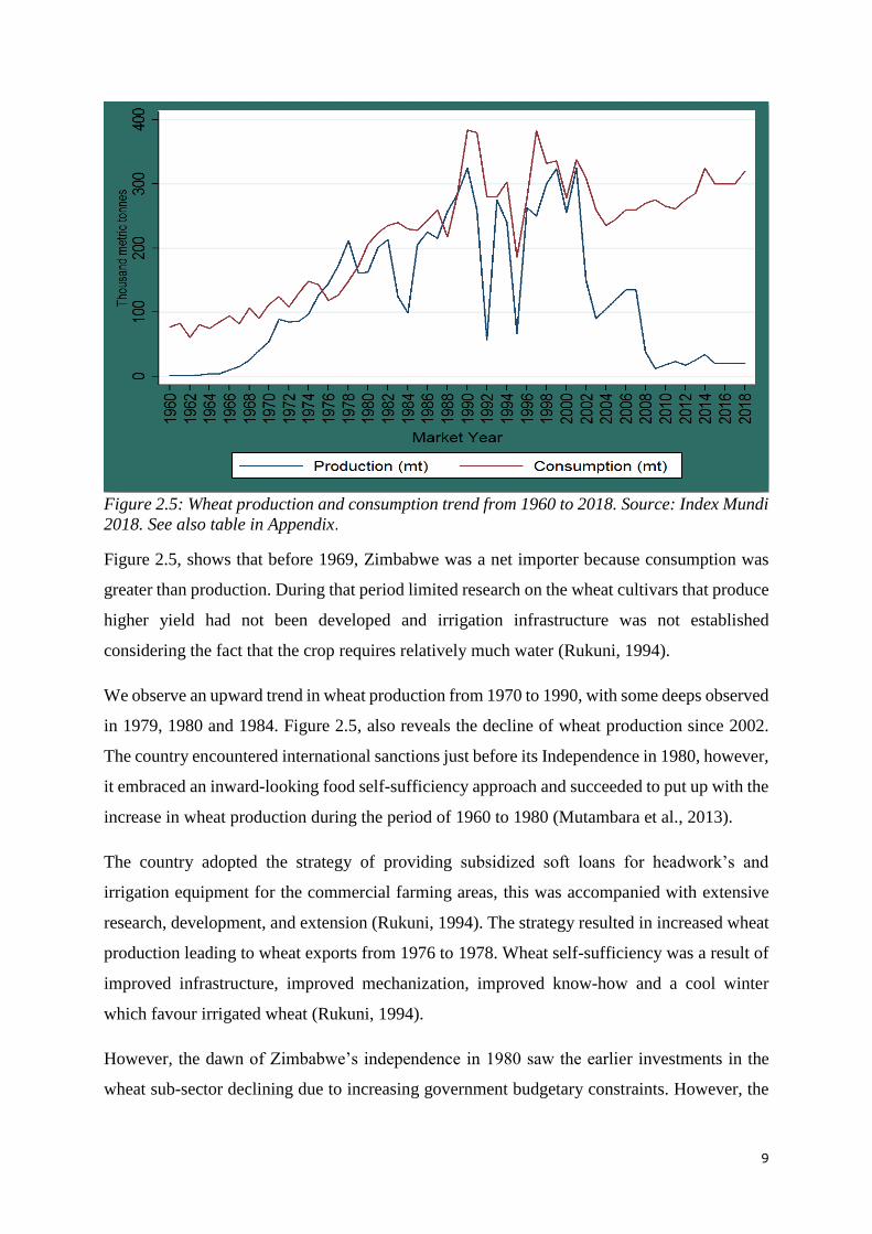
Figure 2.5: Wheat production and consumption trend from 1960 to 2018. Source: Index Mundi
2018. See also table in Appendix.
Figure 2.5, shows that before 1969, Zimbabwe was a net importer because consumption was
greater than production. During that period limited research on the wheat cultivars that produce
higher yield had not been developed and irrigation infrastructure was not established
considering the fact that the crop requires relatively much water (Rukuni, 1994).
We observe an upward trend in wheat production from 1970 to 1990, with some deeps observed
in 1979, 1980 and 1984. Figure 2.5, also reveals the decline of wheat production since 2002.
The country encountered international sanctions just before its Independence in 1980, however,
it embraced an inward-looking food self-sufficiency approach and succeeded to put up with the
increase in wheat production during the period of 1960 to 1980 (Mutambara et al., 2013).
The country adopted the strategy of providing subsidized soft loans for headwork’s and
irrigation equipment for the commercial farming areas, this was accompanied with extensive
research, development, and extension (Rukuni, 1994). The strategy resulted in increased wheat
production leading to wheat exports from 1976 to 1978. Wheat self-sufficiency was a result of
improved infrastructure, improved mechanization, improved know-how and a cool winter
which favour irrigated wheat (Rukuni, 1994).
However, the dawn of Zimbabwe’s independence in 1980 saw the earlier investments in the
wheat sub-sector declining due to increasing government budgetary constraints. However, the
0
50
100
150
200
250
300
350
400
450
196
0
196
2
196
4
196
6
196
8
197
0
197
2
197
4
197
6
197
8
198
0
198
2
198
4
198
6
198
8
199
0
199
2
199
4
199
6
199
8
200
0
200
2
200
4
200
6
200
8
201
0
201
2
201
4
201
6
201
8
Tho
usa
nd
(m
t)
Years
Production (mt)
Consumption (mt)

10
wheat sub-sector enjoyed price subsidy support from 1980 to 2000 to encourage investment in
irrigation and this led to a gradual increase in production (Rukuni et al., 2006).
From 2000 to present domestic consumption surpassed domestic supply (Figure 2.5). The
country shifted from being a net exporter to a net importer of wheat. The country last recorded
exports of 88 000 mt in year 1995, thereafter the production continuously decrease (Appendix
A-I). Domestic demand for wheat has stabilized around 450 000 mt per year, however,
production has dramatically declined from a peak of 325 000 mt in 2001 to 20 000 mt in 2018
(Index Mundi, 2018). Wheat consumption has increased due to an increase in urban population
and changing in preferences thereby widening the gap between production and consumption.
This ultimately enlarge the import demand of the commodity. Since 2000, following the fast-
track land reform program, the drop in production became particularly severe (Mutambara et
al. 2013). The loss of agricultural expertise as well as the decline in investment led to a further
decrease in wheat production (Rukuni, 2006).
The international “economic sanctions” in the 1990s had a negative impact on wheat
production. Economic sanctions are actions taken by foreign countries to limit or terminate their
economic relations with a targeted country for the purpose to persuade that country to change
its behaviour or policies (Chingono, 2010). The economic sanctions caused economic
instability, they also contributed to the isolation of the country from the International
Community. For example, the International Monetary Fund (IMF) withdrew its support to
Zimbabwe in 1999. In addition, the World Bank stopped supporting the infrastructure
development in 2001 (Ministry of Finance, 2003). This has seen an unexpected decline in wheat
production due to lack of funding for expanding the irrigation infrastructure and repairing the
deteriorated equipment. In addition, economic instability resulted in currency problems that
subsequently led the dollarization in 2009. This was an approved replacement of the
Zimbabwean dollar with the U.S. dollar as a result of high inflation (Mpofu, 2015). The
acceptance of the U.S dollar prevented many farmers from planting crops as they did not have
money to purchase seed because the previous year’s crop was sold in Zimbabwean dollars
(USDA, 2009). Hence, this led to the decrease in wheat production in the country.
2.3 Policy issues
From the previous sections plus literature some important policy issues can be identified. These
policy issues will be discussed here.

11
Competition with imports
The position of Zimbabwe of depending on wheat imports means that trade policies have a key
influence on the determination of domestic prices (Kapuya et al., 2010). The local wheat
producer’s performance has turned down due to stringent competition from imports. The
country import wheat from Canada, America, Poland, Turkey and Russia. Being a landlocked
country, imports are mainly delivered through Beira port in Mozambique and then conveyed to
Zimbabwe by rail. Transaction costs of importing are very high and the country faces a rise in
wheat import bills due to increased wheat imports (Mutambara et al., 2013). To lessen the total
reliance on wheat imports, domestic wheat production must be enhanced.
No clear property rights
Farmers in Zimbabwe lease the land from year to year (“A 99-year lease”). This is a legally
binding agreement between government and landholders. However, the lease is not transferable,
making it hard for the farmers to invest more on their farms. Moreover, the government
possesses the power to withdraw the lease from the farmers. This poses a high risk for the
farmer to develop infrastructure on the farm. Farmers have limited decision making powers
regarding the land property (Richardson, 2005).
Lack of credit
As aforementioned, the non- existence of land property rights hinders farmers to access loans
from financial institutions. Lack of international finance opportunities have restricted recovery
of the wheat sector. This led farmers failing to procure inputs in time and repairing irrigation
equipment. Availability of medium to long-term financial credits to farmers positively affect
wheat production (Ahmad et al., 2018). Therefore, a favourable environment is of greater
importance for the farmers to access loans easily and to develop their infrastructure.
Delayed payment by GMB
The GMB is entirely state-owned parastatal. The provision of funds for grain purchases relies
on the government treasury, however the government has fiscal problems and no funds are
being released to GMB (USDA, 2016). Consequently, this led to the delayed payment of
farmers. Because of the delayed payments by GMB, farmers are failing to prepare themselves
well for the next seasons. They cannot access enough funds for inputs procurement. As a result,
thousands of hectares remain unutilised (Richardson, 2005). This coupled with other challenges
has negatively affected wheat production in Zimbabwe.

12
Government Support
Currently, the government is assisting the agricultural sector by pursuing contract farming. To
restore self-sufficiency and to reduce wheat imports, the government intervenes through
Zimbabwe's agro-import substitution programme (Command Agriculture). The country is
driving and expanding the programme as one of its key policies to increase wheat production
(Marufu, 2017). Through the programme, the government supply wheat inputs and repairing
farm machinery hence encouraging more farmers to participate in wheat cropping.

13
Chapter 3: Theory
Introduction
The broad objective of this chapter is to presents the economic theory. The first section of the
chapter illustrates the conceptual framework which provides the theoretical underpinnings of
the research. The second section gives an insight into the analytical technique and production
function. The third section explains short-run profit maximisation and the derivation of the
shadow prices for quasi-fixed inputs. Finally, this chapter concludes by expressing the price
and shadow price equations.
3.1 Conceptual Framework
Figure 3.1 puts forward a number of constraints that influence the supply of wheat. The
framework highlights the cause and effect relationships between wheat supply and its
constraints. Determinants of wheat supply are macroeconomic factors (e.g. exchange rate),
institutional factors (e.g. policy), labour availability and quality, technology and price
expectations. Figure 3.1 shows besides various factors that affect wheat supply that
improvement in wheat supply can lead to wheat self-sufficiency, increase in foreign currency
earnings through a reduction of imports and improved welfare expressed in poverty reduction,
more employment and improved government budget.
Figure 3.1: Factors affecting wheat supply and impacts of improved wheat supply adopted
from (Mahofa 2007).

14
3.2 Analytical technique
Micro-economic theory states that price of a product is the main factor affecting supply. Output
prices play a vital role in the economic system, as it facilitates the allocation of farm resources,
income distribution and encourages farm investment as well as capital development in
agriculture (Chabane, 2002; Shoko et al., 2016). A general increase in the level of product’s
price, ceteris paribus, permits an intensive use of variable inputs, thereby improving crop
production in the country. However, price alone is not the only explanatory variable. Therefore,
price and non-price factors are of paramount importance in the supply function (David, 2013).
Therefore, following the conceptual framework (Figure 3.1), the supply function is made
dependent on macroeconomic factors, institutional factors, the environment, technology, and
weather. These encompasses both price and non-price factors related to production (Key et al.,
2000).
Production function
Taking the prices of the productive factors as given, the producer’s task is to determine the low-
cost combination of factors of production that can produce the anticipated output. This is best
understood in terms of a production function, that expresses the relationship between the
quantities of factors used and the output produced. This can be expressed mathematically as
𝑌 = 𝑓(𝑥1, 𝑥2, 𝐿, 𝐶, 𝐺, 𝑇) where the quantity produced is a function of the combined input
amounts of each factor. In the formula, Y denotes the quantity of output. The producer is
presumed to use 𝑥1𝑎𝑛𝑑 𝑥2 as variable factors of production (for reasons of simplicity we
assume here that there are only two variable inputs), that is, factors which can vary with the
level of production. The producer is also presumed to use quasi-fixed factors, that is, factors
which cannot be varied with the level production in the short run. These includes are 𝐿 labour,
𝐶 capital, 𝐺 land, and 𝑇 technology.
3.4 Profit maximisation
In the short run, costs for quasi-fixed inputs are not relevant for profit maximisation since the
producer cannot change their quantities as they are fixed.

15
Therefore,
max𝑥1,𝑥2
(𝑝 × 𝑓(𝑥1, 𝑥2, 𝐿, 𝐶, 𝐺, 𝑇) − ( 𝑤1𝑥1 + 𝑤2𝑥2)) .............................................................(1)
Where 𝑤1 denotes the price of variable input 𝑥1 and 𝑤2 represents the price of variable input
𝑥2.
To solve a maximisation problem with multiple choice variables:
1. Take the partial derivatives of the function with respect to each variable.
2. Set each partial derivative equal to zero and solve.
First Order Conditions for the variable factors:
𝑝 ×𝜕𝑓(𝑥1,𝑥2,𝐿,𝐶,𝐺,𝑇)
𝜕𝑥1= 𝑤1........................................................................................................(2)
𝑝 ×𝜕𝑓(𝑥1,𝑥2,𝐿,𝐶,𝐺,𝑇)
𝜕𝑥2= 𝑤2........................................................................................................(3)
At the optimal level of each input, the value of the marginal product will equal the price.
First Order Conditions for the fixed factors
𝑝 ×𝜕𝑓(𝑥1,𝑥2,𝐿,𝐶,𝐺,𝑇)
𝜕𝐿= 𝑃𝐿.........................................................................................................(4)
PL denotes the shadow price of labour. As the labour amount cannot be adjusted the shadow
price show the value of labour in the production.
𝑝 ×𝜕𝑓(𝑥1,𝑥2,𝐿,𝐶,𝐺,𝑇)
𝜕𝐶= 𝑃𝐶.........................................................................................................(5)
PC represents the shadow price of capital
𝑝 ×𝜕𝑓𝑥1,𝑥2,𝐿,𝐶,𝐺,𝑇
𝜕𝐺= 𝑃𝐺 .........................................................................................................(6)
PG signifies the shadow price of land
Technology indicates the way inputs are combined into output. we assume it is represented by
the functional relationship between output and inputs. So, we cannot explicitly calculate a
shadow price for it.

16
3.5 Price equations
𝑝 = 𝑝𝑤 × 𝐸𝑅 + 𝑡𝑟𝑝 + 𝑡𝑎𝑝 + 𝑠 .................................................................................................(7)
Where pw -world price of the product, ER- exchange rate, trp - transaction cost, tap-tariffs and s-
subsidies
𝑤1 = 𝑤1𝑤1 × 𝐸𝑅 + 𝑡𝑟𝑤1 + 𝑡𝑎𝑤1 + 𝑠𝑤1...................................................................................(8)
𝑤2 = 𝑤2𝑤2 × 𝐸𝑅 + 𝑡𝑟𝑤2 + 𝑡𝑎𝑤2 + 𝑠𝑤2...................................................................................(9)
Where 𝑤1𝑤1 and 𝑤2𝑤2 are the world prices of the variable factors 1 and 2 respectively, ER-
exchange rate trw1 and trw2 transaction costs, taw1 and taw2 tariffs and 𝑠𝑤1 and 𝑠𝑤2 subsidies on
variable input 1 and 2 respectively.
Therefore, having the prices of the variable inputs and shadow prices of quasi-fixed inputs, an
empirical model can be formulated and solved. Hence, the empirical model for this paper is
built from the above equations. However, to analyse the adjustment of the quasi-fixed factors,
in the long run, the difference between the market price and shadow price of the quasi-fixed
inputs can be determined. The bigger the difference the larger the incentive to adjust the amount
of quasi fixed inputs.
For example, the difference between the shadow price and market price of capital indicates the
incentive to invest or disinvest. If the shadow price is less than the acquisition cost (market
price in case of buying a capital good) this implies that the marginal revenue of a unit of quasi-
fixed input is less than the marginal costs at the acquisition (Drabik and Peerlings, 2018). For
that reason, it is not profitable to expand the use of quasi-fixed inputs.
Furthermore, it is not profitable to sell quasi-fixed inputs if the shadow price is higher than the
salvage value. Salvage value is an estimated resale price of a quasi-fixed input at the end of its
life, i.e. the market price in case of selling a capital good (Adnan and Iqbal, 2018). Conversely,
if the shadow price is higher than the acquisition costs this implies that the marginal revenue of
a unit of quasi-fixed input is higher than the marginal cost at the acquisition. Farmers are likely
to invest when the shadow price of an additional unit of quasi-fixed input surpasses the costs of
acquisition.
Therefore, in the long run, an adjustment in the amount of quasi-fixed inputs is profitable till to
the point where the market price equals the shadow price. Below I give equations for the market
price of labour, capital, and land.
17
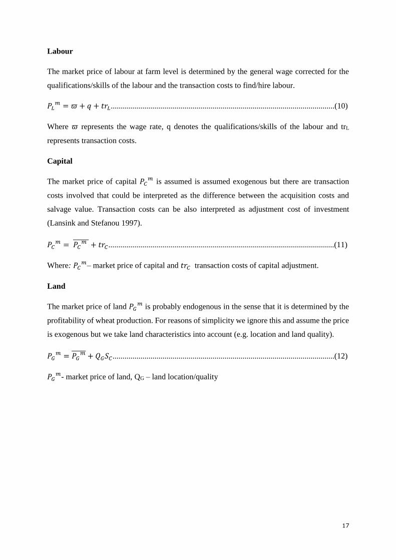
Labour
The market price of labour at farm level is determined by the general wage corrected for the
qualifications/skills of the labour and the transaction costs to find/hire labour.
𝑃𝐿𝑚 = 𝜛 + 𝑞 + 𝑡𝑟𝐿................................................................................................................(10)
Where 𝜛 represents the wage rate, q denotes the qualifications/skills of the labour and trL
represents transaction costs.
Capital
The market price of capital 𝑃𝐶𝑚 is assumed is assumed exogenous but there are transaction
costs involved that could be interpreted as the difference between the acquisition costs and
salvage value. Transaction costs can be also interpreted as adjustment cost of investment
(Lansink and Stefanou 1997).
𝑃𝐶𝑚 = 𝑃𝐶
𝑚 ̅̅ ̅̅ ̅̅ + 𝑡𝑟𝐶.................................................................................................................(11)
Where: 𝑃𝐶𝑚– market price of capital and 𝑡𝑟𝐶 transaction costs of capital adjustment.
Land
The market price of land 𝑃𝐺𝑚 is probably endogenous in the sense that it is determined by the
profitability of wheat production. For reasons of simplicity we ignore this and assume the price
is exogenous but we take land characteristics into account (e.g. location and land quality).
𝑃𝐺𝑚 = 𝑃𝐺
𝑚̅̅ ̅̅ ̅̅ + 𝑄𝐺𝑆𝐶...............................................................................................................(12)
𝑃𝐺𝑚- market price of land, QG – land location/quality

18
Chapter 4 - Data
Introduction
This chapter presents secondary data gathered from different sources. It describes the
variables, data sources and summary statistics.
4.1 Data Sources
Secondary data were collected from multiple sources. First, the domestic producer prices of
both wheat and barley were obtained from the Grain Marketing Board (GMB). Second, the
world prices of wheat were obtained from the United Nations Conference on Trade and
Development Statistics database (UNCTADSTAT). Third, exchange rates and inflation rate
were obtained from the International Monetary Fund through the Federal Reserve Economic
Database. Fourth, yearly data for wheat yield and acreage were obtained from the United States
Department of Agriculture (2017) through the Index Mundi website. Fifth, rainfall data was
obtained from the World Bank database.
4.2 Data
This study uses annual time series data for the period 1965 to 2018 to estimate the wheat supply
response function for Zimbabwe. Table 4.1 reports statistical summaries of the data included in
the study. Specifically, statistical calculations comprising the mean, standard deviation,
minimum and maximum values are presented for each variable.
Table 4.2: Variables
Variable Mean Std. Dev Min Max
Wheat yield (thousand tonnes) 133.87 100.91 4 325
Price of wheat (us$/tonne) 4.00 2.24 1.49 11.01
Price of barley(us$/tonne) 4.24 3.30 1.67 23.73
Exchange rate(zw$/us$) 25.51 111.53 0.57 698.22
World wheat price (us$/tonne) 2.52 0.80 1.61 5.98
Inflation rate (cpi) 568.87 3518.84 0.36 24411.03
Average annual rainfall (mm) 652.71 137.09 411.52 974.87
Acreage (thousand ha) 28.85 16.62 2 57
Land Reform 0.35 0.48 0 1

19
Table 4.2 presents a correlation matrix which shows the correlation coefficients between the
explanatory variables. All prices were converted to real prices using a GDP deflator obtained
from Index Mundi 2018. It is noted that acreage and wheat yield are highly correlated as well
as exchange rates and inflation (Table 4.2).
Table 4.2: Correlation matrix
Exchange
rate
World-
price
Rainfall Acreage Land
reform
Inflation Price of
barley
Price of
wheat
Wheat
yield
Exchange rate 1
World price 0.2483 1
Rainfall -0.0266 0.0835 1
Acreage 0.0107 0.2523 0.283 1
Land reform 0.5764 0.3653 0.1078 0.1388 1
Inflation 0.966 0.3486 -0.0837 0.0807 0.7031 1
Price of barley 0.2121 0.4327 -0.1933 0.2698 0.6642 0.4273 1
Price of wheat 0.3301 0.4176 -0.1361 0.3672 0.6928 0.495 0.8834 1
Wheat yield -0.0725 0.2294 0.2053 0.9549 0.136 0.0037 0.2655 0.4275 1
4.3 Description of variables
Annual domestic wheat yield measured in metric tonnes is used as the dependent (endogenous)
variable. The annual yield is used although winter wheat is harvested only once a year. For the
purpose of consistency and uniformity in the study an average annual wheat yield is used. The
use of wheat yield is besides economic variables influenced by the biological nature of
agricultural production as well as the influence of climate (Ozkan et al., 2011).
The annual domestic producer prices of wheat and barley are independent (exogenous)
variables, they are measured in US dollar per metric tonne. We take yearly prices for wheat and
barley despite that they are harvested only once a year. A positive relationship between wheat
production and price of wheat yield is expected. An increase in the price of a substitute (i.e.
barley) implies a reduction in wheat production (Becker, 2017). Therefore, a negative
relationship is expected between domestic barley prices and total wheat yield.

20
The nominal exchange rate is the price of the Zimbabwean dollar expressed in the US dollar.
US dollar is the main international trading currency in Africa, therefore, it was chosen. In
addition, the annual average was used for consistency and uniformity in the analysis. An
increase in the exchange rate implies a depreciation of the Zimbabwean dollar implying an
increase of the world prices expressed in Zimbabwean dollars. This makes exporting more
attractive and imports more expensive. The bulk of wheat inputs used in wheat production
becomes more expensive and forces farmers to reduce production.
The world price of wheat is another independent variable used in the study to explain the
domestic producer price of wheat in Zimbabwe. World price movements moderately affect
domestic wheat prices (Dasgupta et al., 2011). In order to accurately estimate the price
transmission between the world and domestic prices, the world prices were obtained in US
dollar per metric tonne. Moreover, for consistency, the annual average world prices were used
in the study. An increase in the world price of wheat is expected to put pressure on the country’s
foreign exchange requirements in case of imports, affecting the entire wheat value chain. An
increase in world price increases the import bill which strains foreign exchange more. Wheat
imports decrease consequently, and therefore increase demand for local wheat supply.
Depreciation of the Zimbabwean dollar increases import prices of wheat incentivizing domestic
production.
The annual inflation rate measured as the rate of change of prices (CPI) will be used as an
independent variable. Cost-push inflation occurs when a factor of production’s price increases.
Cost of production as well increases. Consequently, farmers curb their production which in turn
affects supply. Therefore, a negative relationship is expected between the annual inflation rate
and wheat production.
Total annual rainfall expressed in millimetres (mm) per annum and lagged annual average
rainfall recordings will be also used as independent variable. It is expected that annual rainfall
received previous season has a positive effect on total wheat produced. Thus, if abundant rain
is received in the previous year it means that there will be enough water to irrigate wheat in the
next season. The reverse is true in case of drought, which in turn affect wheat production.
Acreage measured in hectares is another independent variable included. This refers to the total
land area employed for wheat production annually. A positive relationship between wheat yield
and area devoted to wheat production is expected.

21
The final independent variable of the study is the dummy which captures the effect of structural
changes generated by the Fast Track Land Reform Programme (FTLRP). FTLRP started in
2000 hence the dummy variable separate two periods (before and after) (Waeterloos and
Rutherford, 2004). The dummy variable takes the value of 0 or 1 to indicate the absence or
presence of the land reform programme. The land invasion had images of theft and irrigation
equipment destruction which dominated the coverage (Scoones et al., 2011). The programme
interfered with normal farm operation in the commercial sector. Therefore, it is expected that
the programme will have a negative and significant effect on wheat yield.
A time trend is another explanatory variable. This variable acts as a proxy for technological
change. Occurrence of a technological change increases the productivity of labour, capital and
other factors of production (Doraszelski and Jaumandreu, 2018). Subsequently, this increases
crop production. Therefore, a positive relationship between wheat yield and technological
change is expected. Since, a rapid adoption of modern technology increases cereal production
(Montgomery and O’Sullivan, 2017).
22
Chapter 5: Empirical Model and Estimation
Introduction
The purpose of this chapter is to present the supply response equation. The first section explains
the empirical model derived from the profit maximising framework. The section further shows
the steps on how to formulate and estimate the reduced form equation. The second section
discusses and presents the final supply response equation.
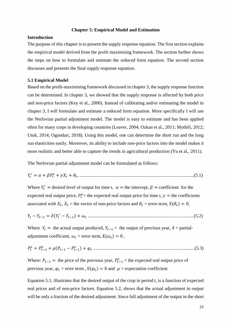
5.1 Empirical Model
Based on the profit-maximising framework discussed in chapter 3, the supply response function
can be determined. In chapter 3, we showed that the supply response is affected by both price
and non-price factors (Key et al., 2000). Instead of calibrating and/or estimating the model in
chapter 3, I will formulate and estimate a reduced form equation. More specifically I will use
the Nerlovian partial adjustment model. The model is easy to estimate and has been applied
often for many crops in developing countries (Leaver, 2004; Ozkan et al., 2011; Mythili, 2012;
Utuk, 2014; Ogundari, 2018). Using this model, one can determine the short run and the long
run elasticities easily. Moreover, its ability to include non-price factors into the model makes it
more realistic and better able to capture the trends in agricultural production (Yu et al., 2011).
The Nerlovian partial adjustment model can be formulated as follows:
𝑌𝑡∗ = 𝛼 + 𝛽𝑃𝑡
𝑒 + 𝛾𝑋𝑡 + 𝜃𝑡, ..................................................................................................(5.1)
Where 𝑌𝑡∗ = desired level of output for time t, 𝛼 = the intercept, 𝛽 = coefficient for the
expected real output price, 𝑃𝑡𝑒= the expected real output price for time t, 𝛾 = the coefficients
associated with 𝑋𝑡, 𝑋𝑡 = the vector of non-price factors and 𝜃𝑡 = error term, E(𝜃𝑡) = 0,
𝑌𝑡 − 𝑌𝑡−1 = 𝛿(𝑌𝑡∗ − 𝑌𝑡−1) + 𝜔𝑡 ...........................................................................................(5.2)
Where 𝑌𝑡 = the actual output produced, 𝑌𝑡−1 = the output of previous year, 𝛿 = partial-
adjustment coefficient, 𝜔𝑡 = error term, E(𝜔𝑡) = 0 ,
𝑃𝑡𝑒 = 𝑃𝑡−1
𝑒 + 𝜇(𝑃𝑡−1 − 𝑃𝑡−1𝑒 ) + 𝜑𝑡 .......................................................................................(5.3)
Where: 𝑃𝑡−1 = the price of the previous year, 𝑃𝑡−1𝑒 = the expected real output price of
previous year, 𝜑𝑡 = error term , E(𝜑𝑡) = 0 and 𝜇 = expectation coefficient.
Equation 5.1, illustrates that the desired output of the crop in period t, is a function of expected
real prices and of non-price factors. Equation 5.2, shows that the actual adjustment in output
will be only a fraction of the desired adjustment. Since full adjustment of the output in the short

23
run may not be feasible. Equation 5.3, specify an equation that explains formation of price
expectations based on actual and past prices. Producers may adjust their expectations as a
fraction (𝜇) of the difference between the actual price and the expected price in the last period
(t-1).The equation to be estimated is obtained through the following steps:
From equation 5.2
𝑌𝑡 − 𝑌𝑡−1 = 𝛿(𝑌𝑡∗ − 𝑌𝑡−1) + 𝜔𝑡
𝑌𝑡 = 𝑌𝑡−1 + 𝛿𝑌𝑡∗ − 𝛿𝑌𝑡−1 + 𝜔𝑡
𝑌𝑡 = 𝛿𝑌𝑡∗ + (1 − 𝛿)𝑌𝑡−1 + 𝜔𝑡...............................................................................................(5.4)
Then, substitute equation 5.1 into 5.4;
𝑌𝑡 = 𝛿[𝛼 + 𝛽𝑃𝑡𝑒 + 𝛾𝑋𝑡 + 𝜃𝑡] + (1 − 𝛿)𝑌𝑡−1 + 𝜔𝑡
𝑌𝑡 = 𝛿𝛼 + 𝛿𝛽𝑃𝑡𝑒 + 𝛿𝛾𝑋𝑡 + 𝛿𝜃𝑡 + (1 − 𝛿)𝑌𝑡−1 + 𝜔𝑡...........................................................(5.5)
From equation 5.3
𝑃𝑡𝑒 = 𝑃𝑡−1
𝑒 + 𝜇𝑃𝑡−1 − 𝜇𝑃𝑡−1𝑒 + 𝜑𝑡
𝑃𝑡𝑒 = 𝜇𝑃𝑡−1 + (1 − 𝜇)𝑃𝑡−1
𝑒 + 𝜑𝑡..........................................................................................(5.6)
Then, substitute equation 5.6 into 5.5
𝑌𝑡 = 𝛿𝛼 + 𝛿𝛽[𝜇𝑃𝑡−1 + (1 − 𝜇)𝑃𝑡−1𝑒 + 𝜑𝑡] + 𝛿𝛾𝑋𝑡 + 𝛿𝜃𝑡 + (1 − 𝛿)𝑌𝑡−1 + 𝜔𝑡
𝑌𝑡 = 𝛿𝛼 + 𝛿𝛽𝜇𝑃𝑡−1 + 𝛿𝛽(1 − 𝜇)𝑃𝑡−1𝑒 + 𝛿𝛽𝜑𝑡 + 𝛿𝛾𝑋𝑡 + 𝛿𝜃𝑡 + (1 − 𝛿)𝑌𝑡−1 + 𝜔𝑡...........(5.7)
We lag equation 5.5 by one period
𝑌𝑡−1 = 𝛿𝛼 + 𝛿𝛽𝑃𝑡−1𝑒 + 𝛿𝛾𝑋𝑡−1 + 𝛿𝜃𝑡−1 + (1 − 𝛿)𝑌𝑡−2 + 𝜔𝑡−1.........................................(5.8)
Multiply equation 5.8 by (1 − 𝜇)
𝑌𝑡−1(1 − 𝜇) = 𝛿𝛼(1- 𝜇) +𝛿𝛽𝑃𝑡−1𝑒 (1- 𝜇) +𝛿𝛾𝑋𝑡−1(1- 𝜇) +𝛿𝜃𝑡−1(1- 𝜇) +(1- 𝜇) (1 − 𝛿)𝑌𝑡−2 +
𝜔𝑡−1 (1- 𝜇) ...................................................................................................(5.9)

24
Then, subtract equation 5.9 from 5.7
𝑌𝑡 − 𝑌𝑡−1(1 − 𝜇)
= 𝛿𝛼 + 𝛿𝛽𝜇𝑃𝑡−1 + 𝛿𝛽(1 − 𝜇)𝑃𝑡−1𝑒 + 𝛿𝛽𝜑𝑡 + 𝛿𝛾𝑋𝑡 + 𝛿𝜃𝑡 + (1 − 𝛿)𝑌𝑡−1 + 𝜔𝑡 – [ 𝛿𝛼(1- 𝜇)
+𝛿𝛽𝑃𝑡−1𝑒 (1- 𝜇) +𝛿𝛾𝑋𝑡−1(1- 𝜇) +𝛿𝜃𝑡−1(1- 𝜇) +(1- 𝜇) (1 − 𝛿)𝑌𝑡−2 + 𝜔𝑡−1 (1- 𝜇)]..........(5.10)
𝑌𝑡 = 𝛿𝛼 + 𝛿𝛽𝜇𝑃𝑡−1 + 𝛿𝛽(1 − 𝜇)𝑃𝑡−1𝑒 + 𝛿𝛽𝜑𝑡 + 𝛿𝛾𝑋𝑡 + 𝛿𝜃𝑡 + (1 − 𝛿)𝑌𝑡−1 + 𝜔𝑡 –
𝛿𝛼 + 𝛿𝛼𝜇 - 𝛿𝛽𝑃𝑡−1𝑒 (1- 𝜇) −𝛿𝛾𝑋𝑡−1(1- 𝜇) −𝛿𝜃𝑡−1(1- 𝜇) −(1- 𝜇) (1 − 𝛿)𝑌𝑡−2 − 𝜔𝑡−1 (1- 𝜇)
+ 𝑌𝑡−1(1 − 𝜇)
𝑌𝑡 = 𝛿𝛼𝜇 + 𝛿𝛽𝜇𝑃𝑡−1 + (1 − 𝛿)(1 − 𝜇)𝑌𝑡−1 − (1 - 𝜇) (1 − 𝛿)𝑌𝑡−2 +𝛿𝛾𝑋𝑡 − 𝛿𝛾(1- 𝜇) 𝑋𝑡−1 +
𝛿𝛽𝜑𝑡 + 𝜔𝑡 −𝛿(1 − 𝜇)𝜃𝑡−1 − (1 − 𝜇)𝜔𝑡−1 + 𝛿𝜃𝑡............................................................(5.11)
The final expression is as follows;
𝑌𝑡 = 𝑏0 + 𝑏1𝑃𝑡−1 + 𝑏2𝑌𝑡−1 + 𝑏3𝑌𝑡−2 + 𝑏4𝑋𝑡 + 𝑏5𝑋𝑡−1 + 휀𝑡............................................(5.12)
Where
𝑏0 = 𝛿𝛼𝜇;
𝑏1 = 𝛿𝛽𝜇,
𝑏2 = ( 1- 𝛿) + ( 1- 𝜇);
𝑏3 = -( 1- 𝛿) (1- 𝜇);
𝑏4 = 𝛿𝛾;
𝑏5 = −𝛿𝛾(1- 𝜇) and
휀𝑡 = 𝜔𝑡 - ( 1- 𝜇) 𝜔𝑡−1+ 𝛿𝜃𝑡 - 𝛿( 1- 𝜇) 𝜃𝑡−1+ 𝛽𝛿𝜑𝑡
Equation 5.12 is a distributed lag model and it includes a lagged dependent variable. However,
it is mostly expressed in natural logarithms to interpret the coefficients easily as the elasticities
(Ogundari, 2018). From equation 5.12, using the coefficient of each independent variable, one
can estimate the short run price response directly, and to obtain the long run price response one
can divide the short run elasticities by adjusted coefficient (Leaver, 2004;Aksoy, 2012).

25
5.2 Estimation
Using the variables selected in the previous chapters, the following function will be estimated:
Supply = 𝑓 (exchange rates, inflation, world prices of wheat, price of barley, price of wheat (t-
1), wheat out-put (t-1) , wheat output (t-2), rainfall (t-1), acreage (t-1), land reform policy,
time trend)
The final equation used is expressed in logarithmic form, this is to ensure the normality of the
residuals. Logarithmic transformation ensures that the errors are normally distributed and
homoscedastic (Maddala, 2001). As highlighted previously, using the logarithmic form allows
also for an easy interpretation of the coefficients as elasticities.
From the correlation matrix in the previous chapter we noted that 𝑜𝑢𝑡𝑝𝑢𝑡𝑡−1 and
𝑎𝑐𝑟𝑒𝑎𝑔𝑒𝑡−1 are highly correlated (0.93) and this led 𝑎𝑐𝑟𝑒𝑎𝑔𝑒𝑡−1 variable to be dropped from
the final model.
Therefore, wheat supply response equation is expressed as:
𝐿𝑜𝑢𝑡𝑝𝑢𝑡𝑡 = 𝑏0 + 𝑏1𝐿𝑟𝑒𝑎𝑙𝑝𝑟𝑖𝑐𝑒𝑡−1 + 𝑏2𝐿𝑜𝑢𝑡𝑝𝑢𝑡𝑡−1 + 𝑏3𝐿𝑜𝑢𝑡𝑝𝑢𝑡𝑡−2 + 𝑏4𝐿𝑒𝑥𝑐ℎ𝑎𝑛𝑔𝑒𝑟𝑎𝑡𝑒𝑡 +
𝑏5𝐿𝑖𝑛𝑓𝑙𝑎𝑡𝑖𝑜𝑛𝑡 + 𝑏6𝐿𝑤𝑜𝑟𝑙𝑑𝑝𝑟𝑖𝑐𝑒𝑡 + 𝑏7𝐿𝑟𝑒𝑎𝑙𝑝𝑟𝑖𝑐𝑒𝑏𝑎𝑟𝑙𝑒𝑦𝑡 + 𝑏8𝐿𝑟𝑎𝑖𝑛𝑓𝑎𝑙𝑙𝑡−1 + 𝑏9𝑙𝑎𝑛𝑑𝑟𝑒𝑓𝑜𝑟𝑚𝑡 +
𝑏10𝑡𝑖𝑚𝑒 + 휀𝑡 .........................................................(5.13)
Where:
𝐿𝑜𝑢𝑡𝑝𝑢𝑡𝑡 = log of total wheat output produced in year t, and measured in tonnes
𝐿𝑟𝑒𝑎𝑙𝑝𝑟𝑖𝑐𝑒𝑡−1 = log of the real wheat price, measured in US dollar per tonne
𝐿𝑜𝑢𝑡𝑝𝑢𝑡𝑡−1 = log of total wheat output lagged by one year
𝐿𝑜𝑢𝑡𝑝𝑢𝑡𝑡−2 = log of total wheat output lagged by two years
𝐿𝑒𝑥𝑐ℎ𝑎𝑛𝑔𝑒𝑟𝑎𝑡𝑒𝑡 = log of the exchange rate in year t
𝐿𝑖𝑛𝑓𝑙𝑎𝑡𝑖𝑜𝑛𝑡 = log of the inflation rate in year t
𝐿𝑤𝑜𝑟𝑙𝑑𝑝𝑟𝑖𝑐𝑒𝑡 = log of the real world wheat price, measured in US dollar per tonne
𝐿𝑟𝑒𝑎𝑙𝑝𝑟𝑖𝑐𝑒𝑏𝑎𝑟𝑙𝑒𝑦𝑡 = log of the real barley price, measured in US dollar per tonne
𝐿𝑟𝑎𝑖𝑛𝑓𝑎𝑙𝑙𝑡−1 = log of the rainfall lagged by one year, expressed in mm
𝑙𝑎𝑛𝑑𝑟𝑒𝑓𝑜𝑟𝑚𝑡 = dummy variable for land reform ( 1 for the years when the policy was
implemented and 0 for the years with no policy)
𝑡𝑖𝑚𝑒 = simple time trend which captures technological change
휀𝑡 = error term

26
Chapter 6: Results
Introduction
The purpose of this chapter is to present the results of the model. The first section discusses
stationarity of the variables in the model. The second section explains if there was a significant
structural change due to the land reform policy. The third section presents and discusses the
estimation results. The fourth section displays the diagnostic tests carried out and their
conclusions. Lastly, this chapter concludes by presenting short and long-run price elasticities.
6.1 Stationarity testing results
The final equation of the Nerlovian model was estimated in Stata using the OLS method. All
variables were tested for stationarity for the period 1965 to 2018. For this test, the Augmented
Dickey-Fuller(ADF) unit root test was used. The stationarity test results are presented in Table
6.1 and 6.2.
Table 6.1: ADF stationarity testing results before differencing.
Variable ADF test
statistic
1% critical
value
5%
critical
value
Probability Conclusion
Acreage 3.441 4.141 3.497 0.057 Non-stationary
Land-reform 3.161 4.143 3.497 1.000 Non-stationary
Exchange rate 1.731 2.639 1.952 0.977 Non-stationary
Inflation 2.868 3.581 2.927 0.057 Non-stationary
Output 3.139 4.14 3.497 0.108 Non-stationary
Output(-1) 3.139 4.141 3.497 0.108 Non-stationary
Output(-2) 3.074 4.144 3.499 0.123 Non-stationary
Rainfall(-1) 6.390 3.563 2.919 0.000 Stationary
Real price of
barley
2.601 3.565 2.919 0.099 Non-stationary
Real price of
wheat (-1)
3.181 4.148 3.500 0.100 Non-stationary
Real-world
price
2.942 3.565 2.919 0.048 Non-stationary
: all variables are in logarithmic form except the dummy trend (land reform).

27
Table 6.2: ADF stationarity testing results at first differences
Variable Test
statistic
1% critical
value
5% critical
value
Probability Conclusion
Acreage 7.37 4.15 3.50 0.0000 Stationary
Inflation 8.67 2.62 1.95 0.0000 Stationary
Output 7.58 4.15 3.50 0.0000 Stationary
Output(-1) 7.58 4.15 3.50 0.0000 Stationary
Output(-2) 7.56 4.15 3.50 0.0000 Stationary
Rainfall(-1) 6.39 3.56 2.92 0.0000 Stationary
Real price of
barley
8.93 2.61 1.95 0.0000 Stationary
Real price of
wheat (-1)
8.54 2.61 1.95 0.0000 Stationary
Real-world
price
6.82 2.61 1.95 0.0000 Stationary
Exchange rate 2.21 4.27 3.56 0.4706 Non-
stationary
Exchange rate-
2nd Difference
6.47 4.263 3.55 0.0000 Stationary
: All variables are in logarithmic form and at first differences.
The results of stationarity tests show that all variables were non-stationary at levels except
rainfall (t-1)(Table 6.1). All other non-stationary variables became stationary after first
differencing apart from exchange rates which became stationary only after second differencing
(Table 6.2). The land reform variable was not corrected for stationarity since it is a dummy
trend.
6.2 Chow-test results
A F-test was used to check if there was a structural change after the implementation of a land
reform policy in year 2000. Land reform policy was treated as a dummy trend variable in this
model. In STATA, the F-test can be carried out using the testparm command. Table 6.3 shows
the results.
Table 6.3: F-test results
Year 2000
H0 : land reform = 0
F- statistic ( 1, 25) = 6.03 P- value = 0.0213
Table 6.3 shows that the outcome of the F-test is 6.03, with p-value 0.0213< 0.05, so it is shown
that we should not leave land reform out from the model. We can reject the null hypothesis.
Therefore, we can conclude that there was a structural change after the impementation of the
land reform policy in 2000 and afterwards.

28
6.3 Wheat supply response results
Table 6.4 presents the regression results of the wheat output response for the period 1965 to
2018. The results show that the R- squared is 0.62, which indicates that explanatory variables
in the model explain 62% of the variation in wheat output. The P-value of F-statistic for wheat
output is 0.0020< 0.05, this suggests overall significance of the relationships in the regression
at 5% level.
The coefficient of lagged output (t-1) had a negative sign with a value of -0.53 The coefficient
is significant at the 5% confidence level, implying that when the country obtains higher wheat
yields, producers tend to reduce the production in the next production season. The law of
demand supply might explains this negative sign. Higher yields may tend to lower the prices of
the crop instigating farmers to react negatively by reducing production in the next season. The
results were similar to those obtained by (Ozkan et al., 2011) who also concluded a negative
relationship between lagged output (t-1) and actual wheat output.
Moreover, the coefficient of lagged output (t-2) had also a negative sign but not significant at
the 10% confidence level, suggesting that the output for the past two years might not
significantly affect the wheat production.
Table 6.4: Regression results for wheat output response from 1965-2018
DEPENDENT VARIABLE: DLoutput
Variables Coefficients Std. Error t-statistic Probability
𝐶𝑜𝑛𝑠𝑡𝑎𝑛𝑡 -4.33 2.56 -1.69 0.103
𝑂𝑢𝑡𝑝𝑢𝑡𝑡−1 -0.53 0.16 -3.31 0.003**
𝑂𝑢𝑡𝑝𝑢𝑡𝑡−2 -0.23 0.15 -1.56 0.130
𝑅𝑒𝑎𝑙 𝑝𝑟𝑖𝑐𝑒 𝑜𝑓 𝑏𝑎𝑟𝑙𝑒𝑦𝑡 -0.04 0.24 -0.16 0.878
𝑅𝑒𝑎𝑙 𝑝𝑟𝑖𝑐𝑒 𝑜𝑓 𝑤ℎ𝑒𝑎𝑡𝑡−1 0.79 0.28 2.87 0.008**
𝑅𝑒𝑎𝑙 𝑤𝑜𝑟𝑙𝑑 𝑝𝑟𝑖𝑐𝑒𝑡 -0.33 0.48 -0.68 0.501
𝐸𝑥𝑐ℎ𝑎𝑛𝑔𝑒 𝑟𝑎𝑡𝑒𝑡 -0.42 0.31 -1.36 0.186
𝐼𝑛𝑓𝑙𝑎𝑡𝑖𝑜𝑛𝑡 -0.18 0.12 -1.52 0.141
𝑇𝑖𝑚𝑒 𝑡𝑟𝑒𝑛𝑑 -0.01 0.01 -1.18 0.249
𝐿𝑎𝑛𝑑𝑟𝑒𝑓𝑜𝑟𝑚𝑡 -0.35 0.14 -2.46 0.021**
𝑅𝑎𝑖𝑛𝑓𝑎𝑙𝑙𝑡−1 0.73 0.39 1.87 0.073*
R2 = 0.62
F-stat = 4.10 (p-value 0.0020 < 0.05)
Observations = 36
**Significant at the 5% level * significant at the 10 %level
As expected, the coefficient for the real price of barley had a negative value of -0.04, since they
are competitive crops. However, the coefficient was not significant at the 10% confidence level.
This implies that the real price of barley had no significant effect on wheat production.
The coefficient of the lagged real price of wheat had a positive sign with a value of 0.79. The
estimated coefficient is significant at the 5% confidence level, implying that the lagged real
price of wheat for the previous season positively influences the wheat production in the next

29
season. These results agree with (Bhatti et al. 2011; Huq et al. 2013) who concluded that there
was a positive relationship between the lagged real price of wheat and its output.
The exchange rate, real-world price, and inflation rate negatively affect wheat production but
they were insignificant at the 10% confidence level, indicating that they insignificantly
influence the production of wheat.
Time trend which was a proxy for technological change. It has a negative sign with the value
of -0.02. The coefficient is not significant at the 10% confidence level. This is not as expected.
However, the time trend may pickup a negative trend in technology for example disinvestment
in irrigation facilities, farm machinery, higher yielding varieties and worse infrastructure.
The dummy trend variable which captures the effect of the land reform policy in year 2000 had
a negative sign with the value of -0.35. The coefficient is significant at the 5% cofidence level.
During landreform process the country experienced high loss of agricultural expertise and the
policy led to the destruction of irrigation facilities and infrastructure (Scoones et al., 2011).
Finally, the results show that lagged rainfall is positively related to wheat output. The
coefficient is significant at the 10 % confidence level. This implies that when the country
recieves more rainfall in the previous season, water sources for example dams and water
resevoirs will have enough water for wheat production in the following season.
6.4 Diagnostic tests
Table 6.5 presents diagnostic tests which were employed to validate the quality of the model.
These tests include a White test for heteroskedasticity, Jarque- Bera test for normality, the
Ramsey RESET test for the stability of the model, and Breusch-Godfrey LM test for
autocorrelation. The table also shows the mean of the variance inflation factor which also shows
the sign of multicollinearity.
Table 6.5: Diagnostic tests results
Testisting for: Method Null-
hypothesis
Outcome P-
value
Conclusion
Heteroskedasticity White
test
Constant
variance
1.88 0.1709 No sign of
heteroskedasticty
Normality Jarque-
Bera test
Normality 0.36 0.8362 Shows residuals
are normally
distributed
Stability Ramsey
RESET
test
Model has no
omitted
variables
3.48 0.1332 No sign of
misspecification
of the model
Autocorelation Breusch
Godfrey
LM test
No serial
autocorrelation
8.38 0.0786 No sign of
autocorelation
Multicollinearrity Mean
VIF
1.98 No serious
problem of
multicollinearity

30
Multicollinearity
To check for severity of multicollinearity, the Variance Inflation Factor (VIF) was obtained
from the STATA output. When there is no collinearity among the explanatory variables VIF
will be equal to 1. VIF index ranges from 1 up to infinity. However, explanatory variables are
said to be highly collinear if their VIF exceeds 10 (Ketema and Kassa, 2016). Table 6.5 shows
that the computed VIF is 1.98 which is very small and the author concludes that there is no
serious problem of multicollinearity. Table 6.6 support that there is no serious correlation
among the explanatory varibles after taking their first differences. However, acreage and lagged
output(t-1) remain highly correlated hence it was dropped from the final model.
Table 6.6: Correlation matrix after first differencing.
Land-
refor
m
Exchange
-rates
Real
world
price
Real
price of
wheat
Real
price
of
barley
Outpu
t (-2)
Outpu
t (-1)
Outpu
t
Inflation Acreag
e
Land-reform 1
Exchange-
rates
0.625 1
Real world
price
0.020 -0.052 1
Real price of
wheat
0.259 -0.028 -0.289 1
Real price of
barley
-0.096 -0.543 0.278 -0.106 1
Output(-2) -0.037 0.0724 0.156 -0.316 0.135 1
Output(-1) -0.202 -0.256 -0.210 -0.092 -0.011 -0.301 1
Output -0.263 -0.101 -0.248 0.434 -0.122 -0.176 -0.277 1
Inflation 0.272 0.273 0.059 -0.075 -0.027 0.077 0.024 -0.307 1
Acreage -0.115 -0.084 -0.182 -0.149 -0.104 -0.295 0.956 -0.283 0.083 1
Figure 6.1 and 6.2 support that there was no sign of heteroskedasticity and also the residuals
were normally distributed.

31
Figure 6.1: No sign of heteroscedasticity
Figure 6.2: Residuals are normally distributed
6.5 Short and long-run price elasticities estimates
Chapter 5 showed that equation 5.12 had to be estimated. However, due to non-stationarity of
the variables, the equation was then estimated in first differences with all variables in
logarithms.
𝑌𝑡 − 𝑌𝑡−1 = 𝑏0 + 𝑏1(𝑃𝑡−1 − 𝑃𝑡−2) + 𝑏2(𝑌𝑡−1 − 𝑌𝑡−2) + 𝑏3(𝑌𝑡−2−𝑌𝑡−3) + 𝑏4𝑋𝑡 + 𝑏5𝑋𝑡−1 + 휀𝑡
𝑌𝑡 = 𝑏0 + 𝑌𝑡−1 + 𝑏1𝑃𝑡−1 − 𝑏1𝑃𝑡−2 + 𝑏2𝑌𝑡−1 − 𝑏2𝑌𝑡−2 + 𝑏3𝑌𝑡−2−𝑏3𝑌𝑡−3 + 𝑏4𝑋𝑡 + 𝑏5𝑋𝑡−1 + 휀𝑡
𝑌𝑡 = 𝑏0 + 𝑏1𝑃𝑡−1 + (1 + 𝑏2)𝑌𝑡−1 + (𝑏3 − 𝑏2)𝑌𝑡−2−𝑏3𝑌𝑡−3 + 𝑏4𝑋𝑡 + 𝑏5𝑋𝑡−1 + 휀𝑡 … … … … . (6.51)
Where 𝑏1 is the short-run price elasticity equalling 0.79, (1 + 𝑏2), (𝑏3 − 𝑏2) and 𝑏3 are the
elasticities of the Outputt−1, Outputt−2 and Outputt−3 respectively. Given that (1 + 𝑏2) = -
0.53 and (𝑏3 − 𝑏2) = -0.23 (Table 6.4). Therefore, 𝑏3 becomes 1.30.
Table 6.6 summaries the estimated short and long-run elasticities. The short-run supply
elasticity is measured by 𝑏1 and the long-run supply elasticity is obtained through dividing the
short run elasticity by the adjustment coefficient. The adjustment coefficient is obtained by
subtracting the coefficient of the lagged dependent variables from 1 (Aksoy, 2012): (Cowling
et al. 2013). Therefore, to calculate the long run elasticity this formula can be applied
𝑏1
(1−(1+𝑏2)−(𝑏3−𝑏2)−𝑏3 =
0.79
(1+0.53+0.23−1.3) =
0.79
0.46 = 1.72

32
The short-run and the long-run price elasticities are estimated as 0.79 and 1.72 respectively. It
is noted that wheat supply is price inelastic in the short run and price elastic in the long run.
This implies that wheat producers adjust their production relatively less than the price changes
in the short run but more than proportional to the price change in the long run.
Table 6.7: Short and long-run price elasticities
Independent variable Short-run elasticity Long-run elasticity
Real wheat price 0.79 1.72
Source: Authors calculation

33
Chapter 7: Discussion and Conclusion
Introduction
The purpose of this chapter is to present the major findings and critically discuss the research.
The first section discusses the major findings of the study. The second section draws the
conclusion of the study based on these findings. Lastly, the chapter provides a critical reflection
and possible solutions to the challenges faced in the study.
7.1 Major Findings
The first research question on describing wheat production and consumption trends has been
answered using literature search. Figure 2.5 in chapter 2, illustrates the trends, showing a
widening gap between production and consumption from the year 1960 to 2018.
From 1966-1974, 1980-1986, and from 1990 to the present domestic consumption surpassed
domestic supply (Figure 2.5). This ultimately increases the import demand of the commodity
which then increases the wheat import bills and further strains the country’s budget.
Figure 7.1, shows the area under wheat production for the period 1965 to 2018. The figure
shows that from 1966-1978 there was a substantial increase in the number of hectares devoted
to wheat production. Thereafter, the area under wheat production started to fluctuate from 1978
to 2006. From 2006 to 2008 the country experienced a sharp drop in the area under production.
It fluctuates again from 2010-2014 and lastly stabilises in 2016 onwards (Figure 7.1).
Figure 7.1:Wheat acreage trend from 1965 to 2018
The estimated supply function indicates that wheat production is affected by both price and
non-price factors. Therefore, this provides answers to the second research question of the study.
The results revealed that lagged real price is one of the factors which affects wheat production.

34
It has a positive impact on the wheat output with an elasticity of 0.79, suggesting that farmers
will venture into wheat production on the basis of the previous price. The results indicate that
a 10% increase in lagged real price of wheat results in 7.9 % and 17% increase in total wheat
output in the short and long run respectively. This concludes that wheat producers adjust their
production relatively more than the price changes in the long run than in the short run. These
results concur with the results from other studies such as (Yunus, 1993; Matin and Alam, 2004;
Begum et al., 2002). Short-run results are in agreement with the results obtained by (Bhatti et
al. 2011) and (Huq et al., 2013). But, the long-run price elasticity results differs.
The lagged output (t-1) is another factor affecting wheat production in Zimbabwe. It has a
negative effect on the wheat output with an elasticity of -0.53, implying that a 10 % increase in
lagged output (t-1) results in a 5.3 % decrease in actual output. Therefore, it is concluded that
the supply conditions of the previous season will affect the production of the next season.
However, these results are in disagreement with the results obtained by (Bhatti et al., 2011))
and (Mann and Warner, 2017)). They find that previous output has a positive impact on actual
wheat output.
The results show that land reform policy which was implemented in the year 2000 is another
determinant of wheat production in Zimbabwe. The results revealed that the policy had a
negative impact on wheat output. This implies that the policy disincentives wheat producers to
a great extent. The implementation of the land reform policy led to the destruction of irrigation
equipment and infrastructure. Moreover, during the land reform process, the land was
redistributed to smallholders farmers with no agricultural expertise and enough capital to
participate in wheat production.
Lastly, lagged rainfall is another important factor that determines wheat production. Rainfall
received in the previous season had a positive impact on wheat produced in the next season.
More rainfall received in the previous year suggests that water sources such as dams and water
reservoirs will be having sufficient water for irrigation in the next season. Similar findings were
obtained by (Mann and Warner, 2017) who concluded that yields are higher in areas with
moderate levels of available water for irrigation. However, in the study by (Huang and Khanna,
2010), their findings were uncertain, they cited that changes in rainfall could lead to an increase
or decrease in wheat yields.

35
7.2 Conclusion
The major objective of this study was to estimate the aggregate wheat supply function for
Zimbabwe from 1965 to 2018. The output response function derived from profit-maximising
was applied to determine the effect of price and non-price factors on wheat production. All
variables were in logarithmic form and were tested for stationarity except for the time trend and
dummy variable. The function was estimated using the Nerlovian partial adjustment model.
Different diagnostic tests applied confirmed the fitness of the model.
As a result, it was established that wheat supply is negatively affected by the output of the
previous season and the land reform programme which was implemented in the year 2000. The
results of the study showed that wheat supply depends on the rainfall of the previous year,
suggesting that sufficient water for wheat irrigation is available if the country receives more
rainfall in the previous season. The findings of the study also revealed that wheat supply is price
inelastic in the short run, implying that farmers are relatively unresponsive to output prices in
the short run, but more responsive in the long run. It is shown that in the long run, the short-run
supply limitations will be resolved and farmers can adjust their level of production to a greater
extent. This could suggest that domestic wheat price support and price stabilisation policy might
influence the wheat supply, but more research is needed to make concrete policy conclusions.
7.3 Critical reflection and possible solutions
This study estimates the aggregate wheat supply function for Zimbabwe using secondary data.
Even though the results are important to the policy makers, in themselves they do not command
policy conclusions. This is because of the limitations of the study. Firstly, the study could not
capture all important variables explained in the theoretical chapter (e.g. fertiliser, labour and
electricity costs) due to lack of data.
Secondly, the study uses aggregate data collected from different sources. Some sources display
different figures of the same variable for example in case of the exchange rates. In addition, the
study focuses only on the aggregate wheat response to price and non-price factors while
possibly there could be a difference in response between farm level and national level.
Thirdly, the effect of the transaction costs explained in the theoretical chapter was also not
captured in the empirical model. Transaction costs which play a key role in the trading of
commodities to determining the implicit and explicit costs of the transaction.

36
Therefore, considering the limitations of the study highlighted above, the following points for
further research were recommended. Instead of using the aggregate data, one can use farm-level
data, implying that primary data will be used in the analysis. By using primary data the author
gains control over the quality and accuracy of the data. Data can also be collected with the
research questions in mind. Moreover, using farm-level data more information can be collected,
thereby increasing the number of variables in the analysis. The effect of variables that differ on
regional and farm level can be investigated e.g. farmer’s expertise. This will enable to formulate
regional policies and target specific groups of farmers.
In addition, there is need to study whether Zimbabwe has a comparative advantage of producing
wheat. More research is clearly needed on specific aspects of this, such as (i) is it an efficient
use of resources for the country to produce wheat? (ii) If it is efficient to produce wheat, what
combination of policy incentives and technological change are needed to promote domestic
wheat production?

37
References
Adnan, M., and M. Iqbal. (2018). Field Performance Evaluation of Indigenous Tractor Mounted
Reaper. Paper read at 2018 ASABE Annual International Meeting.
Ahmad, D., M. Chani, and M. Afzal. (2018). Impact of formal credit on agricultural output:
empirical evidence from Pakistan. Sarhad Journal of Agriculture 34 (3): 640-648.
Aksoy, M. A. (2012). African agricultural reforms: The role of consensus and institutions: The
World Bank.
Anseeuw, W., T. Kapuya, and D. Saruchera. (2011). Draft Zimbabwe Agriculture
Reconstruction: Present state, on-going Projects and Prospects for reinvestment. Study
done for AFD and DBSA. CIRAD, University of Pretoria.
Becker, G. S. (2017). Economic theory: Routledge.
Begum, M., F. Islam, and S. Kamruzzaman. (2002). M., Kabir, MJ and Shiblee, SMA; Supply
Response of Wheat in Bangladesh: An Application of Partial Adjustment Model.
Pakistan Journal of Biological Sciences 5 (2): 225-229.
Bhatti, N., A. A. Shah, N. Shah, F. M. Shaikih, and K. Shafiq. (2011). Supply Response
Analysis of Pakistani Wheat Growers. International Journal of Business and
Management 6 (4): 64.
Chabane, N. (2002). An evaluation of the influences on price and production in the maize
market following liberalisation. Paper read at TIPS Forum.
Chawarika, A., J. Mutambara, and T. Chamboko. (2017). Competitiveness of wheat production
in Zimbabwe. African Journal of Science, Technology, Innovation and Development 9
(3): 263-268. http://dx.doi.org/10.1080/20421338.2017.1322349.
Chingono, H. (2010). Zimbabwe sanctions: An analysis of the Lingo guiding the perceptions
of the sanctioners and the sanctionees. African Journal of Political Science and
International Relations 4 (2): 066-074.
Chinyoka, U. (2013). Analysis of socio-economic factors affecting wheat production in
Zimbabwe: a case of Nyabira, Zvimba district.
Cowling, K., D. Metcalf, and A. Rayner. (2013). Resource structure of agriculture: An
economic analysis: Elsevier.
Dasgupta, D., R. Dubey, and R. Sathish. (2011). Domestic Wheat Price Formation and Food
Inflation in India.
David, B. (2013). Acreage response of rice in Côte D’ivoire: Macro-level response and some
policy implications. International Journal of Agricultural Policy and Research 1 (9):
288-297.

38
Doraszelski, U., and J. Jaumandreu. (2018). Measuring the bias of technological change.
Journal of Political Economy 126 (3): 1027-1084.
Drabik, D., and J. Peerlings. (2018). Economics of Agribusiness [Reader]. Wageningen
Uninversity.
Dzvimbo, M., M. Monga, and T. M. Mashizha. (2017). The link between rural institutions and
rural development: Reflections on smallholder farmers and donors in Zimbabwe.
Journal of Humanities and Social Science 22 (6): 46-53.
Firoozi, A. A., A. A. Firoozi, and M. S. Baghini. (2016). A Review of Clayey Soils. Asian
Journal of Applied Sciences (ISSN: 2321–0893) 4 (06).
Gosalamang, D., A. Belete, J. Hlongwane, and M. Masuku. (2012). Supply response of beef
farmers in Botswana: A Nerlovian partial adjustment model approach. African Journal
of Agricultural Research 7 (31): 4383-4389.
Hove, L., N. Mashingaidze, S. Twomlow, P. Nyathi, M. Moyo, W. Mupangwa, and E.
Masvaya. (2008). Micro Doses, Mega Benefits Promoting Fertilizer Use in Semi-Arid
Zimbabwe. International Crops Research Institute for the Semi-Arid Tropics.
Huang, H., and M. Khanna. (2010). An econometric analysis of US crop yield and cropland
acreage: implications for the impact of climate change. Paper read at AAEA annual
meeting, Denver, Colorado.
Huq, A. A., F. M. Arshad, and G. N. Islam. (2013). Supply response of wheat in Bangladesh:
Cointegration and vector error correction analysis. African Journal of Agricultural
Research 8 (44): 5440-5446.
Index Mundi, (2018), Zimbabwe wheat production by year. Retrieved from
https://www.indexmundi.com/agriculture/?country=zw&commodity=wheat&graph=pr
oduction
Juana, J. S., and R. E. Mabugu. (2005). Assessment of small-holder agriculture's contribution
to the economy of Zimbabwe: A social accounting matrix multiplier analysis. Agrekon
44 (3): 344-362.
Kapuya, T., D. Saruchera, A. Jongwe, T. Mucheri, K. Mujeyi, L. Ndobongo, and F. Meyer.
(2010). The grain industry value chain in Zimbabwe. Unpublished draft prepared for
the Food and Agricultural Organization (FAO). www. fao.
org/fileadmin/templates/est/AAACP/eastafrica/UnvPretoria_GrainChainZimbabwe_2
010_1_. pdf.
39
Ketema, M., and B. Kassa. (2016). Impact of Technology on Smallholder Wheat Production in
Bale Highlands of Ethiopia: Application of Output Decomposition Model. Turkish
Journal of Agriculture-Food Science and Technology 4 (6): 446-454.
Key, N., E. Sadoulet, and A. D. Janvry. (2000). Transactions costs and agricultural household
supply response. American journal of agricultural economics 82 (2): 245-259.
Lansink, A. O., and S. E. Stefanou. (1997). Asymmetric adjustment of dynamic factors at the
firm level. American Journal of Agricultural Economics 79 (4): 1340-1351.
Leaver, R. (2004). Measuring the supply response function of tobacco in Zimbabwe.
Lyons, T., and G. M. Khadiagala. (2010). Conflict management and African politics: ripeness,
bargaining, and mediation: Routledge.
Maddala, G. S.,(2001) Introduction to econometrics. John Willey and Sons Inc.
Maguranyanga, B., and S. Moyo. (2006). Land Tenure in Post FTLRP Zimbabwe: Key Strategic
Policy Development Issues: African Institute for Agrarian Studies Harare.
Mahofa, G. (2007). Economic Analysis of Factors Affecting Cotton Production In Zimbabwe.
Collaborative Masters Program in Agricultural and Applied Economics.
Maiyaki, A. A. (2010). Zimbabwes agricultural industry. African Journal of Business
Management 4 (19): 4159-4166.
Makurira, H. and Viriri, N. (2017). Water permit systems, policy reforms and implications for
equity in Zimbabwe [Report]. Retrieved from http://africa.iwmi.cgiar.org/wp-
content/uploads/sites/2/2017/04/Water-Permitting-Zimbabwe
Mann, M. L., and J. M. Warner. (2017). Ethiopian wheat yield and yield gap estimation: a
spatially explicit small area integrated data approach. Field crops research 201: 60-74.
Marufu, L. (2017 November 30). Command wheat could save country $100 million. The Herald
press. Retrieved from https://www.herald.co.zw/command-wheat-could-save-country-100m/
Matin, M., and S. Alam. (2004). Demand, supply estimation and projection of wheat situation
in Bangladesh. Bangladesh J. Agric. Econ 27 (2): 25-44.
Mlambo, A. S. (2014). A history of Zimbabwe: Cambridge University Press.
Mlambo, K., and N. Zitsanza. (1997). Economies of Scale, Capacity Utilisation and
Productivity Measurement in Zimbabwean Commercial Agriculture. African
Development Review 9 (2): 15-32.
Mohanty, S., S. K. Nayak, B. Kaith, and S. Kalia. (2015). Polymer nanocomposites based on
inorganic and organic nanomaterials: John Wiley & Sons.
Montgomery, J., and F. O’Sullivan. (2017). Spatial variability of tight oil well productivity and
the impact of technology. Applied Energy 195: 344-355.

40
Morris, M. L. (1988). Comparative advantage and policy incentives for wheat production in
Zimbabwe.
Moyo, S. (2011). Three decades of agrarian reform in Zimbabwe. Journal of Peasant Studies
38 (3): 493-531.
Mpofu, R. T. (2015). Dollarization and economic development in Zimbabwe: An interrupted
time-series analysis. Risk Governance & Control: Financial Markets & Institutions 5
(4): 38-48.
Mushunje, A., and A. Belete. (2001). Efficiency of Zimbabwean small scale communal farmers.
Agrekon 40 (3): 344-360.
Mutambara, J. and Zvinavashe, A. (2012). Wheat value chain and business environmental
factors in Zimabwe. University of Zimbabwe.
Mutambara, J., A. Zvinavashe, and E. Mwakiwa. (2013). A critical review of the wheat industry
in Zimbabwe. Global Journal of Biology, Agriculture and Health Sciences, GJBAHS 2:
23-33.
Mythili, G. (2012). Acreage and yield response for major crops in the pre-and post-reform
periods in India: A dynamic panel data approach.
Negassa, A., B. Shiferaw, J. Koo, K. Sonder, M. Smale, H. Braun, S. Gbegbelegbe. (2013). The
potential for wheat production in Africa: analysis of biophysical suitability and
economic profitability.
Nyamangara, J., L. Mugwira, and S. Mpofu. (2000). Soil fertility status in the communal areas
of Zimbabwe in relation to sustainable crop production. Journal of Sustainable
Agriculture 16 (2): 15-29.
Ogundari, K. (2018). Maize supply response to price and nonprice determinants in Nigeria:
bounds testing approach. International Transactions in Operational Research 25 (5):
1537-1551.
Ozkan, B., R. F. Ceylan, and H. Kizilay. (2011). Supply response for wheat in Turkey: A vector
error correction approach. New Medit 3: 34-38.
Richardson, C. J. (2005). The loss of property rights and the collapse of Zimbabwe. Cato J. 25:
541.
Rukuni, M. (1994). "Impact of smallholder irrigation in Zimbabwe." In.: Faculty of Agriculture,
University of Zimbabwe (UZ).
Rukuni, M. (2006). Revisiting Zimbabwe’s agricultural revolution. Zimbabwe’s Agricultural
Revolution Revisited, Harare, Zimbabwe: University of Zimbabwe Publications.

41
Rukuni, M., P. Tawonezvi, C. Eicher, M. Munyuki-Hungwe, and P. Matondi. (2006).
Zimbabwe’s agricultural revolution revisited. University of Zimbabwe Publications,
Harare: 119-140.
Scoones, I., N. Marongwe, B. Mavedzenge, F. Murimbarimba, J. Mahenehene, and C. Sukume.
(2011). Zimbabwe's land reform: challenging the myths. Journal of Peasant Studies 38
(5): 967-993.
Shoko, R., P. Chaminuka, and A. Belete. (2016). Estimating the supply response of maize in
South Africa: a Nerlovian partial adjustment model approach. Agrekon 55 (3): 237-253.
Toringepi, G. (2016). The contribution of smallholder agriculture production to food security
in rural Zimbabwe: a case study of Masvingo Province, University of Fort Hare.
USDA. (2009). Zimbabwe Gain Report. Retrieved from
https://ipad.fas.usda.gov/highlights/2009/06/zimbabwe/
Utuk, I. (2014). Aggregate Agricultural Output Supply Response in Akwa Ibom State of
Nigeria: An Application of the Nerlovian Adjustment Model. Journal of Agriculture
and Veterinary Science 7 (9): 22-33.
Waeterloos, E., and B. Rutherford. (2004). Land reform in Zimbabwe: challenges and
opportunities for poverty reduction among commercial farm workers. World
Development 32 (3): 537-553.
Yu, B., F. Liu, and L. You. (2011). Dynamic agricultural supply response under economic
transformation: a case study of Henan, China. American Journal of Agricultural
Economics 94 (2): 370-376.
Yunus, M. (1993). Farmers' Response to Price in Bangladesh. The Bangladesh Development
Studies 21 (3): 101-109.
World Bank. (2017). Zimbabwe Economic Update, June 2017 : The State in the Economy.
https://openknowledge.worldbank.org/handle/10986/27474 License: CC BY 3.0 IGO.”
ZAIP. (2017). A comprehensive framework for the development of Zimbabwe agriculture
sector.
ZINWA. (2014). Understanding the water permit and water agreement systems in Zimbabwe.
Retrieved from https://www.zinwa.co.zw/understanding-the-water-permit-and-water-
agreement-systems-in-zimbabwe/

42
APPENDIX A:
Table A-1:Zimbabwe Wheat production, Consumption, Imports, Acreage, Yield /ha and
Exports
Market YearProduction (1000 MT) Consumption(1000MT) Imports(1000 MT) Acreage (1000HA) Yield MT/HA) Exports(1000MT)
1960 1 77 79 1 1 3
1961 1 83 85 1 1 3
1962 1 61 64 1 1 4
1963 2 81 83 1 2 4
1964 4 75 73 1 4 2
1965 4 85 85 2 2 4
1966 10 94 84 5 2 0
1967 15 82 67 5 3 0
1968 25 107 82 7 4 0
1969 40 90 58 12 3 0
1970 54 112 77 15 4 0
1971 89 124 55 23 4 0
1972 85 108 20 24 4 0
1973 86 130 65 22 4 0
1974 97 148 42 26 4 0
1975 126 143 12 32 4 0
1976 145 118 10 34 4 0
1977 173 127 0 45 4 1
1978 212 148 0 48 4 2
1979 161 172 0 37 4 8
1980 162 206 3 35 5 5
1981 201 224 17 43 5 0
1982 213 235 30 37 6 0
1983 124 240 71 23 5 0
1984 99 230 104 20 5 0
1985 205 228 86 42 5 0
1986 225 243 53 43 5 0
1987 215 260 75 40 5 0
1988 257 217 14 47 5 20
1989 284 284 8 50 6 0
1990 325 384 65 55 6 11
1991 259 380 0 46 6 0
1992 57 280 170 12 5 0
1993 275 280 33 47 6 3
1994 240 303 78 43 6 1
1995 67 186 157 18 4 88
1996 263 278 75 48 5 0
1997 250 383 133 52 5 0
1998 300 332 32 50 6 0
1999 324 336 12 57 6 0
2000 255 278 23 46 6 0
2001 325 338 13 45 7 0
2002 150 310 110 38 4 0
2003 90 260 170 30 3 0
2004 105 235 130 35 3 0
2005 120 245 125 35 3 0
2006 135 260 125 35 4 0
2007 135 260 125 45 3 0
2008 38 270 200 9 4 0
2009 12 275 250 4 3 0
2010 18 265 250 5 4 0
2011 23 261 250 12 2 0
2012 17 275 250 9 2 0
2013 25 285 250 10 2 0
2014 34 325 300 15 2 0
2015 20 300 280 10 2 0
2016 20 300 280 10 2 0
2017 20 300 280 10 2 0
2018 20 320 300 10 2 0
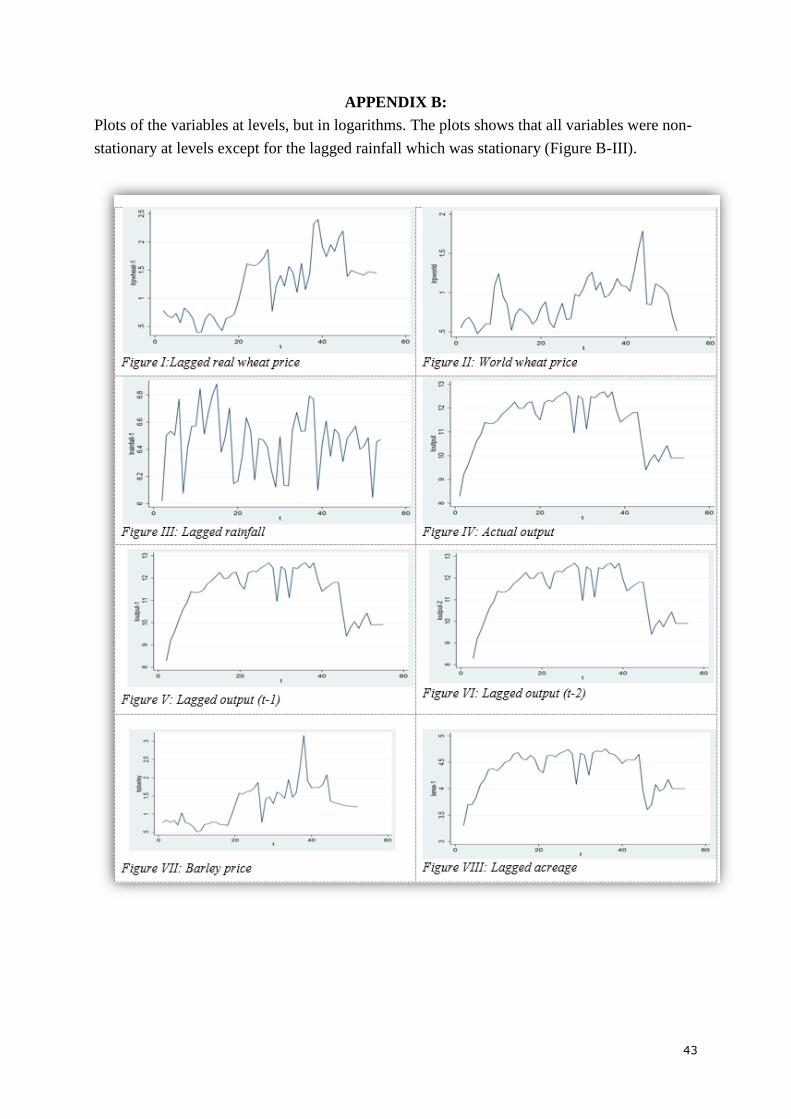
43
APPENDIX B:
Plots of the variables at levels, but in logarithms. The plots shows that all variables were non-
stationary at levels except for the lagged rainfall which was stationary (Figure B-III).

44

45
APPENDIX C
Soil status in Zimbabwe
By analysing Table I and Figure I, the country is dominated by soils of Order Kaolinitic. The
Order comprises Fersiallitic, Paraferrallitic and Orthoferrallitic soils. These soils are mainly
formed from granite rocks which is the parent material for the sandy soils. This implies that
sand to sandy loam soils mainly dominates the country (Hove et al., 2008). Sandy soils are
inherently infertile with low soil organic matter (SOM) and susceptible to leaching. The
kaolinite soils dominate in Natura region I, II, III, and IV. Kaolinite soils have low Cation
Exchange Capacity (CEC) (Mohanty et al., 2015). CEC refers to a soil chemical property which
acts as soil fertility indicator. It shows the ability of the soil to hold and supply plant nutrients.
Therefore, soils with high sand content have low CEC, implying that they supply less plant
nutrients (Firoozi et al., 2016).
The majority of the smallholder farmers are located in sandy soils and these farmers have
limited resources and limited agricultural expertise which hinders effective crop production in
the country (Nyamangara et al., 2000). As explained in chapter 2, wheat production is mainly
practiced in Mashonaland Central, Mashonaland East and Mashonaland West provinces, these
provinces fall in Natural region I,II and III mostly. But, these regions are dominated by sandy
to sandy loam soils with less organic content and susceptible to leaching (Hove et al., 2008).
Therefore, it is highly recommended to add organic and inorganic fertilisers to boost soil
fertility. Nitrogen (N) and phosphorus(P) are the nutrients identified to limit crop production in
Zimbabwe (Hove et al., 2008). Hence, to increase crop yields by smallholder farmers
appropriate amount of fertiliser or manure need to be applied.
Soil classification in Zimbabwe
Table 3:Soil classification in Zimbabwe
Order Description Group Typical soil
families
Agro
ecological
zone
dominated
AMORPHIC
Very little or no
horizon development
1. Lithosol-
very shallow
soils
2. Regosol-
deep and
extremely
low silt/clay
ratios
Derived
from mafic
rocks
Deep sands
derived
from
Kalahari
desert
Region IV
western and
Northern
parts
CALIMORPHIC Unleached soils with
large reserves of
weatherable minerals
3. Vertisols –
moderately
deep to deep
clay soils and
acidic
Derived
from basalt
and mafic
rocks
Region V
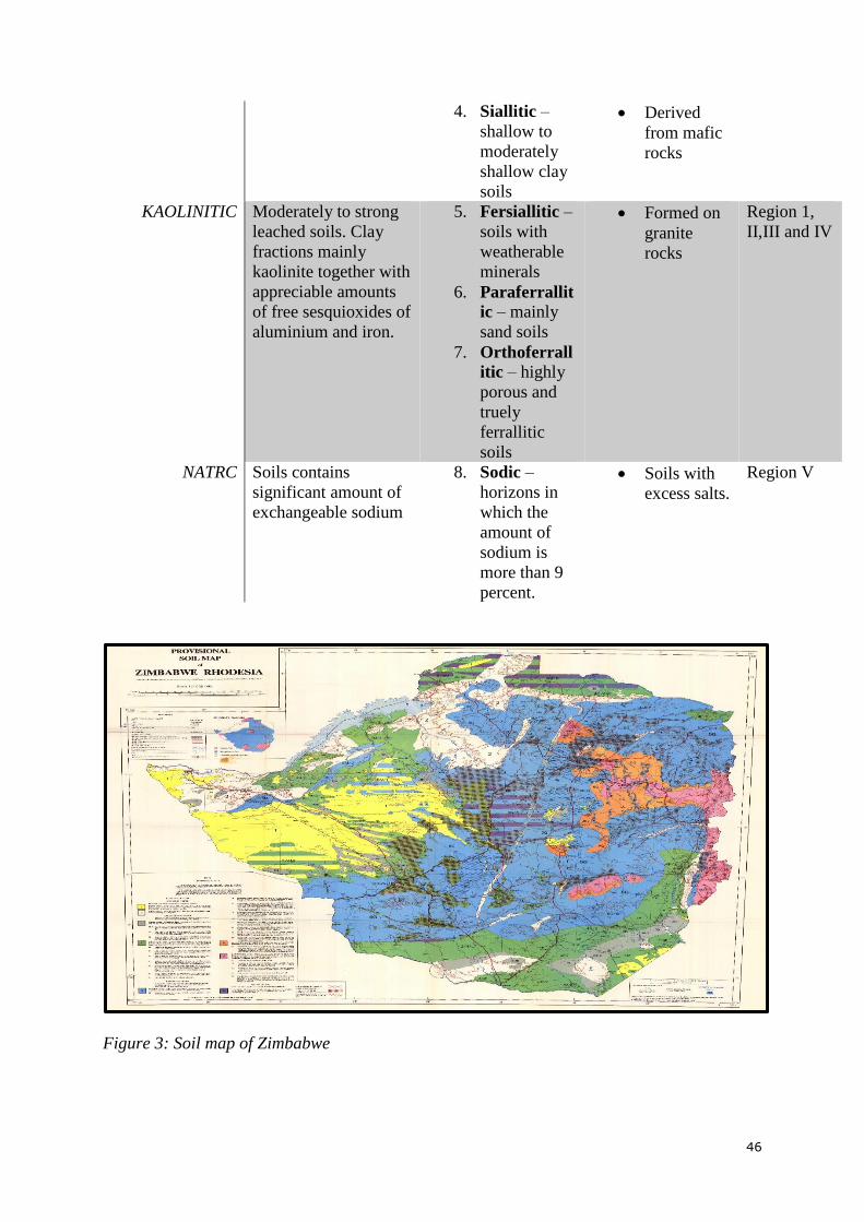
46
4. Siallitic –
shallow to
moderately
shallow clay
soils
Derived
from mafic
rocks
KAOLINITIC Moderately to strong
leached soils. Clay
fractions mainly
kaolinite together with
appreciable amounts
of free sesquioxides of
aluminium and iron.
5. Fersiallitic –
soils with
weatherable
minerals
6. Paraferrallit
ic – mainly
sand soils
7. Orthoferrall
itic – highly
porous and
truely
ferrallitic
soils
Formed on
granite
rocks
Region 1,
II,III and IV
NATRC Soils contains
significant amount of
exchangeable sodium
8. Sodic –
horizons in
which the
amount of
sodium is
more than 9
percent.
Soils with
excess salts.
Region V
Figure 3: Soil map of Zimbabwe

47
APPENDIX D
Water availability
Access to water is free only for basic use. Farmers who intend to use water from rivers and
dams for irrigation purposes (commercial use) are required to obtain water permits from the
Zimbabwe National Water Authority (ZINWA). Water permits help in safeguarding the
interests and allocations of permit holders. For example in times of water scarcity, farmers with
permits will be given priority to use water before new water users are taken. However, farmers
holding water permits are required to pay for the water use and this affect winter crop
production to a greater extent because most smallholder farmers are not able to pay for the water
bills for irrigation (ZINWA, 2014).
Figure 2 below shows the water catchment areas in Zimbabwe. ZINWA divided the country
into seven water catchment areas which includes; Gwayi, Mazoe, Mzingwane, Runde, Sanyati,
Save and Manyame. These are considered to be more effective accountability units for water
use. Each catchment area comprises of permanent rivers and dams which intend to supply water
to local farmers. The provinces where wheat production is mainly practiced are being water
supplied by Manyame, Mazoe, Sanyati, Save, and Runde (Figure 2).
Figure 4:Water catchment areas in Zimbabwe: (Makurira and Viriri, 2017)

48
APPENDIX E
Money supply
In 2009, Zimbabwe officially adopts the U.S. dollar as its currency. The introduction of the
U.S dollar shows a significant change in the stability of the economy (Mpofu, 2015). From
2009 to 2015 Zimbabwean economy started to normalise gradually. But, in the first quarter of
2016, cash shortages re-surfaced and the Reserve Bank of Zimbabwe introduced the bond notes
to solve the problem. Bond notes were given the same value as the U.S dollar. However, bond
notes were not legalised to be used outside Zimbabwe. The present situation implies that
Zimbabwe is trading with two types of currency; the foreign currency and the local currency.
The Government officials insisted that the two currency is at par, but, on the black market, they
have two different values. The foreign currency shortages worsened to the extent that it is only
found on the black market, suggesting hyper-inflation in the country. This causes prices of
inputs such as fertilizers, seed and agro-chemicals to rise as the currency loss value. Therefore,
this continue to hinder wheat production in the country.