An efficient algorithm for gene/species treesparsimonious reconciliation with losses,

duplications and transfers

Jean-Philippe Doyon1, Celine Scornavacca2, K. Yu. Gorbunov3, Gergely J.Szollosi4, Vincent Ranwez5, and Vincent Berry1

1 LIRMM, CNRS - Univ. Montpellier 2, France.2 Center for Bioinformatics (ZBIT), Tuebingen Univ., Germany.

3 Kharkevich IITP, Russian Academy of Sciences, Moscow.4 LBBE, CNRS - Univ. Lyon 1, France.

5 ISEM, CNRS - Univ. Montpellier 2, France.

Abstract. Tree reconciliation methods aim at estimating the evolution-ary events that cause discrepancy between gene trees and species trees.We provide a discrete computational model that considers duplications,transfers and losses of genes. The model yields a fast and exact algorithmto infer time consistent and most parsimonious reconciliations. Then westudy the conditions under which parsimony is able to accurately infersuch events. Overall, it performs well even under realistic rates, transfersbeing in general less accurately recovered than duplications. An imple-mentation is freely available at http://www.atgc-montpellier.fr/MPR.

1 Introduction

Duplications, losses and transfers are evolutionary events that shape genomesof eukaryotes and prokaryotes. They result in discrepancy between gene andspecies trees. Tree reconciliation methods aim at estimating the course of theseevents in order to explain the observed incongruence of gene and species trees.A reconciliation defines an embedding of a gene tree G into a species tree Straditionally represented as a set of tubes. Localized duplications, transfers andlosses are induced by the chosen embedding. These methods find applicationsin various areas such as identification of orthologous sequences for functionalannotation in genomics [3], coevolutionary studies in ecology [10], and studieson poputation areas in biogeography.

Probabilistic models have been proposed to reconcile trees [15, 13], but heavycomputing times still limit their use to relatively small sets of taxa and smallcollections of genes. An alternative approach relies on the more tractable com-binatorial principle of parsimony [4]. Yet, with the advent of next generationsequencing technologies, that flood molecular biology with new genomes, evencombinatorial methods might become too computationally expensive to han-dle phylogenomic databases, that regularly deal with several dozen thousandsof gene families [11]. In this paper, we propose a combinatorial reconciliationmethod that has the potential to keep pace with new sequencing technologies.

More formally, we consider the Most Parsimonious Reconciliation (MPR)problem: given a species tree S, a gene tree G and respective costs for duplication,transfer and loss events (respectively denoted D, T, and L events), compute atime-consistent reconciliation that has a minimum cost. Time consistency meansthat T events happen only horizontally, i.e. between coexisting species, and thecost of a reconciliation is the sum of the costs of the events implied by theembedding of G into S. For instance, when D, T, and L events have cost 5, 10, 1respectively, the reconciliation of Fig. 1 (left) costs 23.

When only DLS events are considered (S refers to a speciation), the MPRproblem can be solved in linear time w.r.t. the size of G for binary trees [17].The problem remains tractable when S is polytomous, and it can be solved inO(|G|·(dS +hS)) time, where hS is the height of S and dS is the size of its largestpolytomy [16]. However, when T events are also considered, the MPR problemhas been proven to be NP-complete, even for reconciling a single binary gene treewith a binary species tree [14]. This strong contrast in complexity is explainedby the difficulty of managing the chronological constraints among nodes of Sthat are induced by T events. When not constraining T events, time inconsistentscenarios can ensue, such as that of Fig. 1 (right), as remarked in [6]. A promisingapproach is to alter the definition of MPR to accept a dated tree S as input [9,1, 10, 5, 15]. Dates for nodes of S can be obtained by relaxed molecular clocktechniques working from gene trees and molecular sequences. For the purpose ofreconciliation, dates only need to be relative to one another, hence they are littlelimited by the possible absence of fossil records for the studied species [8]. Givena dated tree S, time consistency can be ensured locally by only considering T

events whose donor and receiver branches have intersecting time intervals [10].However, two locally consistent T events can be globally inconsistent (Fig. 1;right), which then needs to be fixed by altering afterwards the position of theproposed T [10], but this approach does not guarantee to solve MPR exactly.To ensure global consistency, branches of S can be subdivided into time slicestransversal to all edges. Then, slices are explored one after the other, and onlycombinations of T events in a same time slice are considered. This recently ledto exact algorithms running in O((|S| · |G|)4) [7] and O(|S|3 · |G|) [5], i.e. whosecomplexity still needs to be improved for phylogenomic purposes.

To that aim, we propose here a partially different modelization that leads toan exact algorithm solving the time consistent MPR problem for a dated speciestree in O(|S′|·|G|), where S′ is a subdivision of S in at most O(|S|2) nodes. Then,we rely on an implementation of this fast algorithm to obtain a first insight forthe question: Is parsimony relevant to infer the true evolutionary scenario of agene family?

2 Methods

2.1 Basic definitions and notations

Let T be a tree with nodes V (T ) and branches E(T ), and such that only itsleaves are labeled. Let r(T ), L(T ), and L (T ) respectively denote its root node,

the set of its leaf nodes, and the set of taxa labelling its leaves. We will adopt theconvention that the root is at the top of the tree and the leaves at the bottom.

An edge of T is denoted (u, v) ∈ E(T ), where u is the parent of v. For a nodeu of T , Tu denotes the subtree of T rooted at u, up its parent, (up, u) its parentedge, and T(up,u) denotes the subtree of T rooted at edge (up, u). Given a subsetof leaves K ⊆ L(T ), the homeomorphic tree of T connecting K, denoted TK , isthe smallest binary tree induced from T such that L(TK) = K.

An internal node u of T has one or two children, where {u1} and {u1, u2}respectively denote its child set. It is important to point out that because T isan unordered tree, the children u1 and u2 of u are interchangeable. Given twonodes u, u′ of T , u′ is said to be a (resp. strict) descendant of u if u is on thepath from u′ to r(T ) (resp. and u 6= u′). An internal node u of T is said to beartificial when it has a unique child. Contracting an artificial node means thatthe node is removed from the tree and that its two adjacent edges are merged.A tree T ′ is said to be a subdivision of a tree T if the recursive contraction ofall artificial nodes of T ′ yields T .

A species tree S is a rooted binary tree such that each element of L (S) repre-sents an extant species labeling exactly one leaf of S (there is a bijection betweenL(S) and L (S)). S is associated with a time stamp function θS : V (S) → R. Thisfunction ensures that ∀x ∈ L(S), θS(x) = 0 and for any two nodes x, x′ ∈ V (S),if x′ is a strict descendant of x then θS(x′) < θS(x). A gene tree G is a rootedbinary tree. From now on, we consider a species tree S and a gene tree G suchthat L (G) ⊆ L (S) and where L : L(G) → L(S) denotes the function that mapseach leaf of G to the unique leaf of S with the same label. To distinguish betweenG and S, the term edge refers to G and the term branch refers to S.

We introduce below the concept of a scenario describing the evolution of agene that starts at node r(S) and evolves along S according to DTLS events.Such a scenario generates a completed gene tree denoted Go, whose leaf set isformed of contemporary genes (denoted LC(Go)) but also of lost genes (denotedLL(Go)), see Fig. 1 and 2. Note that L(Go) = LC(Go) ∪ LL(Go).

Definition 1. Given an observed gene tree G and a species tree S, with its timestamp function θS, a DTLS scenario for G along S is denoted (Go, M, θo

G), whereGo is a completed gene tree, M : V (Go) → V (S) maps each node of Go to a nodeof S, and θo

G : V (Go) → [0, θS(r(S))] associates each node of Go to a time stamp

z

A B C D

x x′ x′′

yy′

a1 b1 c1 d1

u

w

t1

t2

z

A B C D

x x′ x′′

yy′

a1 b1 c1 d1

u

w

t1

t2

t3t4

Fig. 1: Two scenarios for a gene tree G (plain lines) along a species tree S (tubes),where the symbol ◦ represents loss. (Left) A time consistent scenario. (Right) Ascenario that is not time consistent: the transfer from the donor at t3 (resp. t4)to a receiver at t1 (resp. t2) implies that u predates (resp. follows) w.

of S. The scenario associates a DTLS event to each node u ∈ V (Go) \ LC(Go)as follows (denoting x = M(u)):

1. If u is a leaf of LL(Go), then it corresponds to an L event.2. If M(u1) = x1, and M(u2) = x2, then u is an S event happening at x in S′.3. If M(u1) = x and M(u2) = x, then u is a D event along the branch (xp, x).4. If M(u1) = x, M(u2) = y, and y is neither an ancestor nor a descendant of

x, then u is a T event, where (xp, x) and (yp, y) respectively correspond tothe donor and the receiver branches.

A DTLS scenario is said to be consistent if and only if the following con-straints are respected. First, the homeomorphic gene tree Go

LC(Go) is G. Second,

for a T event (described above in (4)), [θS(x), θS(xp)]∩[θS(y), θS(yp)] 6= ∅. Third,for each edge (up, u) ∈ E(Go), θo

G(up) > θoG(u).

The cost of such a scenario is denoted Cost(Go, M, θoG) = dδ+ tτ + lλ, where

d, t, and l respectively denote the number of D, T, and L events, and δ, τ , andλ are their respective costs.

Consider a species tree S with a time stamp function θS , an observed genetree G, the leaf-association function L : L(G) → L(S), and costs δ, τ , resp. λ forD, T resp. L events. Given these inputs, the optimization problem consideredin the present paper, called MPR, is to compute a consistent DTLS scenario(Go, M, θo

G) for G along S that minimizes Cost(Go, M, θoG).

2.2 A tractable model of reconciliation

To obtain a tractable model, we discretize time by subdividing the species treeinto time slices (see Fig. 3; similarly as done in [1, 13]), then define a limitednumber of cases for events to happen, that still allows us to infer a most parsi-monious scenario.

Definition 2. Given a species (binary) tree S and a time stamp function θS :V (S) → R, let S′ be the subdivision of S constructed as follows: for each nodex ∈ V (S) \L(S) and each branch (yp, y) ∈ E(S) s.t. θS(yp) > θS(x) > θS(y), an

r(G)

a1 b1c1 d1

u w

r(Go)

a1 b1c1 d1

u w

Fig. 2: (Left) An observed gene tree G with four leaves a1, b1, c1, and d1, re-spectively belonging to the contemporary species A, B, C, and D (see Fig. 1).(Right) A completed gene tree Go, with L(Go) = LC(Go) ∪ LL(Go), whereLC(Go) = {a1, b1, c1, d1}, and LL(Go) is formed of the two nodes labelled ◦.G is the homeomorphic tree Go

K , where K = LC(Go).

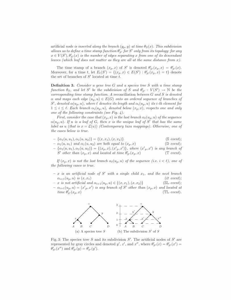
artificial node is inserted along the branch (yp, y) at time θS(x). This subdivisionallows us to define a time stamp function θ′S′ for S′ only from its topology: for anyx ∈ V (S′), θ′S′(x) is the number of edges separating x from one of its descendantleaves (which leaf does not matter as they are all at the same distance from x).

The time stamp of a branch (xp, x) of S′ is denoted θ′S′(xp, x) = θ′S′(x).Moreover, for a time t, let Et(S

′) = {(xp, x) ∈ E(S′) : θ′S′(xp, x) = t} denotethe set of branches of S′ located at time t.

Definition 3. Consider a gene tree G and a species tree S with a time stampfunction θS, and let S′ be the subdivision of S and θ′S′ : V (S′) → N be thecorresponding time stamp function. A reconciliation between G and S is denotedα and maps each edge (up, u) ∈ E(G) onto an ordered sequence of branches ofS′, denoted α(up, u), where ℓ denotes its length and αi(up, u) its i-th element for1 ≤ i ≤ ℓ. Each branch αi(up, u), denoted below (xp, x), respects one and onlyone of the following constraints (see Fig. 4).

First, consider the case that (xp, x) is the last branch αℓ(up, u) of the sequenceα(up, u). If u is a leaf of G, then x is the unique leaf of S′ that has the samelabel as u (that is x = L(u)) (Contemporary taxa mappings). Otherwise, one ofthe cases below is true.

– {α1(u, u1), α1(u, u2)} = {(x, x1), (x, x2)} (S event);– α1(u, u1) and α1(u, u2) are both equal to (xp, x) (D event);– {α1(u, u1), α1(u, u2)} = {(xp, x), (x′

p, x′)}, where (x′

p, x′) is any branch of

S′ other than (xp, x) and located at time θ′S′(xp, x) (T event).

If (xp, x) is not the last branch αℓ(up, u) of the sequence (i.e. i < ℓ), one ofthe following cases is true.

– x is an artificial node of S′ with a single child x1, and the next branchαi+1(up, u) is (x, x1) (∅ event);

– x is not artificial and αi+1(up, u) ∈ {(x, x1), (x, x2)} (SL event);– αi+1(up, u) = (x′

p, x′) is any branch of S′ other than (xp, x) and located at

time θ′S′(xp, x) (TL event).

A B C D

x

y

z

(a) A species tree S

A B C D0

1

2

3

x

y

z

x′ x′′

y′

(b) The subdivision S′ of S

Fig. 3: The species tree S and its subdivision S′. The artificial nodes of S′ arerepresented by gray circles and denoted y′, x′, and x′′, where θ′S′(x) = θ′S′(x′) =θ′S′(x′′) and θ′S′(y) = θ′S′(y′).

A reconciliation α between the gene tree G of Fig. 2 (left) and the subdivisionS′ of Fig. 3b is depicted in Fig 1(left), where the path α(w, b1) along S′ associatedto the edge (w, b1) is [(y, x′), (y′, x), (x, B)]. Observe that the extended gene treeGo (see Fig. 2; right) is a by-product of the reconciliation α.

Note that T events only happen between branches in a same time slice, henceonly time-consistent scenarios are generated by this model. We now argue thatthe model allows to infer most parsimonious scenarios (see Def. 1). First, notethat each loss is coupled with either a speciation (SL) or a transfer (TL). Indeed,any most parsimonious reconciliation embedding G into S′ only needs to use aloss when it meets a speciation node of S′ where G goes into only one descendingtube, or when leaving a tube due to a transfer, with no part of G remaining inthe donor tube. Considering a lone loss as a seventh event in Fig. 4 would lead toexamine reconciliations that are not most parsimonious, as this would only allowto replace – in a Go tree generated by the current model – a single l ∈ LL(Go) bya subtree with no extant species (as the structure of G is common to both thesecompleted gene trees). Such a subtree contains at least two losses and is henceless parsimonious than leaving leaf l in the Go proposed with the current model.Then, any combination of DTLS events resulting from a scenario (Def 1) can bereproduced by the model of Def. 3, safe for combinations that would obviouslynot lead to most parsimonious scenarios: a speciation of a gene where its twosons go extinct before reaching the leaves of S′; a gene duplication where at leastone of its sons goes extinct; a transfer where the transfered gene lineage goesextinct.

Last, remark that all cases considered in Def. 3 (see Fig. 4) allow to progresseither in the time slices of S′ or along the edges of G, safe for the TL case, but forwhich possible following events must be of a different kind in a most parsimoniousscenario (see Prop. 1 in appendix). Thus, the model offers all ingredients fora dynamic programming algorithm that finds a most parsimonious and timeconsistent scenario, while still running in time polynomial in |S′| and |G|. Inother words, this model allows to solve the MPR problem exactly and in atractable way.

Note that since the model places each loss immediately after another event(speciation or transfer), it is not able to generate a most parsimonious scenarioσ = (Go, M, θo

G) where a lineage is lost after being alive for several slices ina same tube (without meeting a speciation node). However, it can generate ascenario σ′ = (Go, M , θo

G) that can be seen as a canonical representative of σ:both scenarios share the same Go and have the same number and localization ofD, T, and L events in S (σ and σ′ only differ in the position of some L in thesubdivided species tree S′).

2.3 An efficient algorithm to solve MPR

In this section, we propose a polynomial time and space algorithm that usesthe tractable reconciliation model of Def. 3 to solve the MPR problem (seeAlgorithm 1).

PSfrag

u

u2u1

x1 x2

x

xp

(a) Speciation (S)

u

u2u1

x

xp

(b) Duplication (D)

u

u2u1

x

xp x′p

x′

(c) Transfer (T)

u

x

x1

xp

(d) ∅ event

u

x1 x2

x

xp

(e) Speciation + Loss (SL)

u

x

xpx′

p

x′

(f) Transfer+Loss (TL)

Fig. 4: The six DTLS events of Def. 3, where an edge (up, u) of Go is mapped ontoa branch (xp, x) of the sequence α(up, u). The extended gene tree Go is embeddedin the subdivision S′ of a species tree S, where an edge of G corresponds to aplain line, a branch of S′ corresponds to a dotted tube (white zone), and a nodeof S′ corresponds to a gray zone.

Consider an edge (up, u) ∈ E(G), a branch (xp, x) ∈ E(S′), and the timet = θ′S′(xp, x). Let Cost(u, x) denote the minimal cost over all reconciliationsbetween G(up,u) and the forest of subtrees of S′ rooted with a branch locatedat time t, and such that (xp, x) is the first branch in the sequence associatedto (up, u) (that is α1(up, u) = (xp, x); see Def. 3). Assuming that the gene treeG and the species tree S are rooted with an artificial branch, Cost(r(G), r(S′))corresponds to the minimal cost over all reconciliations between G and S. Thedynamic programming algorithm (see pseudo-code in Algorithm 1) fills the ma-trix Cost : V (G) × V (S′) → N through two embedded loops: one that visitsall edges according to a bottom-up traversal of G and one that visits all timestamps of S′ in backward time order (i.e. starting from 0). For the edge (up, u)and the time stamp t currently considered (respectively in lines 3 and 4), twoconsecutive loops over all branches (xp, x) ∈ Et(S

′) compute the minimal cost ofmapping (up, u) onto (xp, x) according to the six events S, D, T, ∅, SL, and TL

(see Fig. 4). For a branch (xp, x) ∈ Et(S′), the first loop (lines 5 to 20) computes

the minimal cost among the first five events, the second loop (lines 21 to 24)computes that for the TL event, and Cost(u, x) is the minimum of these twovalues.

The case of Fig. 4c is considered at lines 13 to 15 where the cost of a T eventstarting at (xp, x) is computed for edge (up, u). Assuming that (u, u1) (resp.(u, u2)) is the transfered gene lineage, a subroutine called BestReceiver computes

Algorithm 1 Computes Cost(r(G), r(S′)) according to the DTL costs, respec-tively denoted δ, τ , and λ.

1: Construct the subdivision S′ of S as described in Def. 22: The matrix Cost : V (G) × V (S′) → N is initialized as follows: if u ∈ L(G),

x ∈ L(S′), and L(u) = x, then Cost(u, x)← 0. Else, Cost(u, x)←∞.

3: for all (up, u) ∈ E(G) according to a bottom-up traversal do

4: for all t∈{0, 1, . . . , θ′S′(r(S′))} in backward time order do

5: for all branch (xp, x) ∈ Et(S′) do

6: if u ∈ L(G), x ∈ L(S′), and L(u) = x then

7: Skip lines 8 to 20 and go to the next iteration of the loop at line 5{Basecase}

8: Costg ←∞, for each g ∈ {S, D, T, ∅, SL}

9: if u has two children then

10: if x has two children then

11: CostS ← min{Cost(u1, x1)+Cost(u2, x2), Cost(u1, x2)+Cost(u2, x1)}

12: CostD ← Cost(u1, x) + Cost(u2, x) + δ

13: (yp, y)← BestReceiver((u, u1), t, (xp, x))

14: (zp, z)← BestReceiver((u,u2), t, (xp, x))

15: CostT ← min{ Cost(u1, x) + Cost(u2, z), Cost(u1, y) + Cost(u2, x) }+ τ

16: if x has a single child then

17: Cost∅ ← Cost(u, x1)

18: if u has two children then

19: CostSL ← min{Cost(u, x1), Cost(u, x2)}+ λ

20: Cost(u, x)← min{Costg : g ∈ {S, D, T, ∅, SL}}

21: for all branch (xp, x) ∈ Et(S′) do

22: (x′p, x′)← BestReceiver((up, u), t, (xp, x))

23: CostTL ← Cost(u, x′) + τ + λ

24: Cost(u, x)← min{ Cost(u, x), CostTL }

25: return Cost(r(G), r(S′))

the branch (yp, y) (resp. (zp, z)) that minimizes Cost(u1, y) (resp. Cost(u2, z))over all branches of S′ located at the same time t, other than (xp, x). The samesubroutine is used at line 22 for the TL case of Fig. 4f. A similar optimizationto compute the optimal receiver for a transfer was found independently in [13].

Algorithm 1 computes the cost of a most parsimonious reconciliation. Back-tracking in the computations of values in the dynamic programming table yieldsa most parsimonious reconciliation (in the sense of Def. 3), which readily allowsto obtain a most parsimonious scenario (see Def. 1), as we argued in Section. 2.2.See Appendix for details on the achievable complexity.

Theorem 1. The MPR problem can be solved in Θ(|S′| · |G|) time and space.

3 Experimental Results

To asses the performance of parsimony, we calculated the most parsimoniousreconciliations for a large scale simulated data set that was obtained using aprobabilistic model of duplication, transfer, and loss. In our simulations, westarted with a single gene at the root of the species tree and generated gene treesaccording to a Poisson process characterized by rates of duplication, transferand loss. We compiled two different data sets called ds1 and ds2, aiming bothto simulate a relatively large phylogenetic time scale (a bacterial or archeanphylum) with realistic loss rates as well as to explore a wide range of duplicationand transfer rates. For further details on ds1 and ds2, see the Appendix.

For each data set, we used a single cost per event corresponding to the inverseof the average rate of this event during the simulation process (i.e., for ds1

δ = 1/0.18). According to those costs and for each pair of gene and species trees,we used Algorithm 1 to compute one of the most parsimonious reconciliationsdenoted αp.

Note that the real reconciliation αR may contain the record of events thatcannot be recovered by a reconciliation for G, since no traces of them exist. Forinstance, subtrees whose leaves are all lost, D events followed straightaway by anL event, or several TL events in a row. Thus, we post-processed the DTL eventsof αR, removing hidden parts of αR of the above kinds, but potentially leavingother unrecoverable parts that are more complex to detect. This leads to obtaina reconciliation α′

R.We first study under which conditions the parsimony criterion can correctly

estimate the DTL events that lead to the obtention of an observed gene treeG. This can be simply achieved by comparing the costs of the real scenarioand that of a most parsimonious one. As soon as the two costs strongly differ,the parsimony is no longer a reasonable approach. Recall that the cost of areconciliation α can be computed as Cost(α) = dδ + tτ + lλ, where d, t and lare the number of D, resp. T, resp. L implied by α. The relative over cost ofα′

R in terms of parsimony score compared to that of a most parsimonious one isdefined below:

OverCost(α′R, αP ) =

Cost(α′R)− Cost(αP )

Cost(αP ).

Note that if Cost(α′

R) = Cost(αP ), this does not imply that αP = α′

R sinceseveral most parsimonious scenarios can exist. Fig. 5 shows the extent of thisover cost depending on the duplication and transfer rates and tree heights. Wecan see that the over cost is really small for all combinations of duplication andtransfer rates we investigated, but does increase with the height of the gene trees.This can be related to hidden events that we failed to identify and remove fromα′

R.We now proceed to investigate quantitatively whether parsimony is able to

correctly infer the position of DTL events.Recall that a reconciliation α of a gene tree G defines DTL events associated

to internal nodes and edges of G. As the position of duplication and transferevents in Go allow to locate losses, we only focus below on D and T events. Let

D(α) ⊆ V (G) \ L(G) denote the subset of internal nodes of G that correspondto a D event and T(α) ⊆ E(G) the subset of edges of G that correspond to a T

event. It is important to point out that D(α) and T(α) alone do not resolve wherein S the event has taken place, hence are not sufficient to determine whether aDTL event is common to two reconciliations. Let DS(α) denote the set of pairs(u, (xp, x)) ∈ D(α) × E(S) such that α places u on the branch (xp, x) of S. LetTS(α) denote the triplet set ((up, u), (xp, x), (yp, y)) ∈ T(α) × E(S)2 such that(up, u) is a T event from the donor (xp, x) to the receiver (yp, y) branches in S.

Given a most parsimonious reconciliation αP , its accuracy to retrieve the D

and T events of the real (simulated) reconciliation α′

R is evaluated by the ratiosof false positive and false negative events defined as follows:

FPE(α′R, αP ) =

|ES(αP )−ES(α′

R)|

|ES(αP )|

FNE(α′R, αP ) =

|ES(α′

R)−ES(αP )|

|ES(α′

R)|

,

where E = D, T. Figures 6 and 7 show those ratios for various combinationsof D, T rates and tree heights.

In Fig. 6, we can see that FPD is close to zero for all combinations of duplica-tion and transfer rates we investigated. This means that almost all parsimoniousduplications are correct (i.e., present in α′

R). The high values of FND can be ex-plained by several reasons. First, α′

R can contain hidden events that cannot bedetected by reconciliation approaches. Second, fixing δ = τ causes the misiden-tification of some D events replaced by T events in the inference. This wouldalso explain the high ratio of false positive transfers with such rates (see Fig. 7).Finally, this can be due to the fact that we chose the wrong most parsimoniousreconciliation among the several possible ones. This also explains the quite highlevel of false negatives for T events.

4 Conclusion

We presented a new model for reconciling gene and species trees. This modelleads to a fast and exact algorithm to compute a time consistent and most par-

0

0.1

0.2

0.3

0.4 0.5

0.6

0.05 0.1 0.15 0.2 0.25 0.3

0.2 0.4

0.8

1.6

0 0.1 0.2 0.3 0.4 0.5 0.6

TH 0.05

0.15 0.25

0.35 0.05

0.15 0.25

0.35

0 0.1 0.2 0.3 0.4 0.5 0.6

ove

r co

st

TD

(a) (b)

ove

r co

st

Fig. 5: Over cost of simulated scenarios compared to that of most parsimoniousones for combinations of heights, transfer and duplication rates, i.e. ds1 (a) andds2 (b). High values show cases where parsimony criterion is inadequate.

0.05 0.1 0.15 0.2 0.25

0.3

0.2

0.4

0.8

1.6

0 0.1 0.2 0.3 0.4 0.5 0.6

FN

D

TH

0 0.1 0.2 0.3 0.4 0.5 0.6

0.05 0.1 0.15 0.2 0.25 0.3

0.2

0.4

0.8

1.6

0 0.1 0.2 0.3 0.4 0.5 0.6

FP D

TH 0.05

0.15 0.25

0.35

0.05 0.15

0.25

0.35

0 0.1 0.2 0.3 0.4 0.5 0.6

FP D

TD

0.05 0.15

0.25 0.35

0.05

0.15

0.25

0.35

0 0.1 0.2 0.3 0.4 0.5 0.6

FN

D

TD

(a) (b)

(c) (d)

Fig. 6: Accuracy of parsimony to estimate reconciliations: ratios of false negative(a,b) and false positive (c,d) to estimate and localize D events, for combinationsof heights, transfer and duplication rates, i.e. ds1 (a,c) and ds2 (b,d).

(a) (b)

(c) (d)

0.05 0.15

0.25 0.35

0.05

0.15

0.25 0.35

0 0.1 0.2 0.3 0.4 0.5 0.6

FN

T

TD

0.05 0.15

0.25 0.35

0.05

0.15

0.25

0.35

0 0.1 0.2 0.3 0.4 0.5 0.6

FP T

TD 0.05 0.1 0.15 0.2 0.25 0.3

0.2

0.4

0.8

1.6

0 0.1 0.2 0.3 0.4 0.5 0.6

0 0.1 0.2 0.3 0.4 0.5 0.6

TH

TF

NT

FP

0.05 0.1 0.15 0.2 0.25 0.3

0.2

0.4

0.8

1.6

0 0.1 0.2 0.3 0.4 0.5 0.6

TH

Fig. 7: Accuracy of parsimony to estimate reconciliations: ratios of false negative(a,b) and false positive (c,d) to estimate and localize T events, for combinationsof heights, transfer and duplication rates, i.e. ds1 (a,c) and ds2 (b,d).

simonious reconciliation while accounting for duplications, losses and transfers.Simulations showed that the parsimony criterion performs satisfactorily underrealistic conditions at the phylum level. At the inter-phlyum level, transfers aremore difficult to recover and the existence of several most-parsimonious reconcil-iations might be a decisive factor there. This needs further scrutiny. Moreover,running times are on average 1.09s (resp. 1.38s) for low (resp. high) rates ofevents for trees on 100 species. This clearly scales the reconciliation approach upto the phylogenomic stage, where several tens of thousand genes are considered.

Many things remain to be done, among others to allow for multifurcating geneand species trees and to measure the accuracy of the reconciliation approach fororthology prediction (where the localization of events is not needed, increasingthe accuracy of the method w.r.t. results of Section 3) compared to other relevantmethods in this context.

References

1. C. Conow, D. Fielder, Y. Ovadia, and R. Libeskind-Hadas. Jane: a new tool for thecophylogeny reconstruction problem. Algorithms Mol Biol, 5:16, 2010.

2. M. Csuros and I. Miklos. Streamlining and Large Ancestral Genomes in Archaea Inferredwith a Phylogenetic Birth-and-Death Model. Mol Biol Evol, 26(9):2087–2095, 2009.

3. Toni Gabaldon. Computational approaches for the prediction of protein function in themitochondrion. Am J Physiol Cell Physiol, 291(6):C1121–1128, 2006.

4. M. Goodman, J. Czelusniak, G. W. Moore, Romero A. Herrera, and G. Matsuda. Fittingthe gene lineage into its species lineage, a parsimony strategy illustrated by cladogramsconstructed from globin sequences. Syst. Zool., 28:132–163, 1979.

5. K. I. Gorbunov and V. A. Lyubetsky. Reconstructing genes evolution along a species tree.Mol. Biol. (Mosk.), 43:946–958, 2009.

6. M. Hallett, J. Lagergren, and A. Tofigh. Simultaneous identification of duplications andlateral transfers. In RECOMB ’04, pp. 347–356, New York, NY, USA, 2004. San Diego,California, USA, ACM.

7. R. Libeskind-Hadas and M. A. Charleston. On the computational complexity of thereticulate cophylogeny reconstruction problem. JCB, 16(1):105–117, 2009.

8. S.P. Loader, D. Pisani, J.A. Cotton, D.J. Gower, J.J. Day, and M. Wilkinson. Relativetime scales reveal multiple origins of parallel disjunct distributions of african caecilianamphibians. Biol Lett., pp. 505–508, October 2007.

9. D. Merkle and M. Middendorf. Reconstruction of the cophylogenetic history of relatedphylogenetic trees with divergence timing information. Theory Biosci, 123(4):277–299,2005.

10. D. Merkle, M. Middendorf, and N. Wieseke. A parameter-adaptive dynamic programmingapproach for inferring cophylogenies. BMC Bioinformatics, 11(Suppl 1):S60, 2010.

11. S. Penel, A. M. Arigon, J. F. Dufayard, A. S. Sertier, V. Daubin, L. Duret, M. Gouy,and G. Perriere. Databases of homologous gene families for comparative genomics. BMCBioinformatics, 10 Suppl 6:S3, 2009.

12. A. Rambaut. Phylogen: phylogenetic tree simulator package, 2002.13. A. Tofigh. Using Trees to Capture Reticulate Evolution, Lateral Gene Transfers and

Cancer Progression. PhD thesis, KTH Royal Institute of Technology, Sweden, 2009.14. A. Tofigh, M. Hallett, and J. Lagergren. Simultaneous identification of duplications and

lateral gene transfers. IEEE/ACM TCBB, 99, 2010.15. A. Tofigh, J. Sjostrand, B. Sennblad, L. Arvestad, and J. Lagergren. Detecting LGTs

using a novel probabilistic model integrating duplications, lgts, losses, rate variation, andsequence evolution, Manuscript.

16. B. Vernot, M. Stolzer, A. Goldman, and D. Durand. Reconciliation with non-binaryspecies trees. J. Comput. Biol., 15:981–1006, 2008.

17. L. Zhang. On a mirkin-muchnik-smith conjecture for comparing molecular phylogenies.Journal of Computational Biology, 4(2):177–187, 1997.

A Author contributions

CS, JP, KG and VB discussed ideas in existing reconciliation algorithms. JP,VB, VR proposed the new reconciliation model. CS, JP, VB and VR designedthe algorithm. CS implemented the MPR algorithm and the reconciliation com-parisons. GS implemented the reconciliation simulator. CS and GS performedsimulations, designed and analyzed in collaboration with JP,VB and VR. CS,GS, JP, VB and VR wrote the manuscript.

B Some proofs

Property 1. Consider a parsimonious reconciliation α between G and S, an edge(up, u) of G and a time t. The sequence α(up, u) contains at most two branchesof S′ located at time t. If there are two such branches denoted αi(up, u) andαj(up, u), then they are adjacent in the sequence α(up, u) (i.e. |i − j| = 1).

Proof The adjacency of the two branches follows immediately from Def. 3(relying on the fact that both happen at time t).

Assume that α contains two TL events for (up, u) described as follows: thereare three adjacent branches αi(up, u), αi+1(up, u) and αi+2(up, u) in Et(S

′),which respectively corresponds (according to Def. 3) to the donor of the firstTL event, the receiver (resp. donor) of the first (resp. second) TL event, and thereceiver of the second TL event.

As the cost of a single TL event between αi(up, u) and αi+2(up, u) is smallerthan the cost for the previous two TL events, α is not a parsimonious reconcili-ation. �

Proof of the complexity of the algorithm

Proof of the time complexity. We claim the algorithm runs in O(n′m) wheren′ is the size of the subdivides species tree S′ and m is the size of G.

The loop over the edges of G (line 3) runs for Θ(m) iterations. The loop overthe times t of S′ (line 4) together with the two loops over branches Et(S

′) insequence (line 5 and 21) run for Θ(n′) iterations. Thus, lines 6 to 20 and lines22 to 24 are run Θ(n′m) time globally. For the nodes u ∈ V (G) and x ∈ V (S′)currently visited, we now have to prove that Cost(u, x) can be computed inconstant time, which is obviously the case for the cost associated to the S, D, ∅,and SL events (see lines 11, 12, 16, and 18, respectively). We prove below howthe cost associated to a T event (lines 13 to 15) can be computed in constanttime, considering that both genes are conserved (we omit the case for a TL

combination at lines 22 to 24, as it is solved using the same optimization idea).Consider a T event from a donor (xp, x) ∈ Et(S

′), assuming w.l.o.g. that(u, u1) is conserved in the lineage (xp, x) while (u, u2) is transfered. The algo-rithm needs to compute the optimal receiver (i.e. that leading to a minimum

cost) for (u, u2) in Et(S′) \ {(xp, x)}. As currently stated, i.e. in the most read-

able form, Algorithm 1 allows to compute the best receiver in Θ(|Et(S′)|) time

by a simple loop over the branch set Et(S′) (line 14; subroutine BestReceiver).

However, slightly modifying the statement of the algorithm allows to computethe best receiver in constant time at line 14 (and similarly lines 13 and 22). Toachieve this, immediately before the loop over the branch set Et(S

′) (line 5),add another loop on Et(S

′) to find the first and second optimal receivers for(u, u2) in Et(S

′) and denote (x′

p, x′) and (x′′

p, x′′) these respective receivers.

Second, when a donor (xp, x) ∈ Et(S′) is visited during the loop at line 5, the

optimal receiver for (u, u2) in Et(S′) \ {(xp, x)} is the first optimal receiver if

(xp, x) 6= (x′

p, x′), and the second one otherwise. Hence line 13 now requires con-

stant time, while adding the additional loop mentioned above doesn’t cost morethan the already existing loop of line 5. As a result, the overall time complexityof the algorithm is in Θ(n′m).

Proof of the space complexity. The size of the whole matrix Cost(u, x) is inΘ(n′m), all other variables used in the algorithm are constant in size, and thespace complexity is then immediate. �

Sketch of the proof for the correctness of the algorithm

Given a tree T , define the height of a node u ∈ V (T ), denoted h(u), as the lengthof the unique path from u to r(T ), and the height of T , denoted h(T ), is themaximal height over all its nodes.

Consider the edge (up, u) and the time stamp t examined at an iteration ofthe main loops (respectively in lines 3 and 4) in the algorithm. For any branch(xp, x) ∈ Et(S

′), we now explain how the two loops compute Cost(u, x) byconsidering all six events seperately. First, for the S and D events (lines 11and 12 resp.), the consistency of the corresponding cost is ensured because forany child u′ ∈ {u1, u2} and any branch (x′

p, x′) of S′, Cost(u′, x′) is previously

computed during the bottom-up traversal of G. Second, for the ∅ and SL events(lines 17 and 19 resp.), the optimality is verified because for any branch (x′

p, x′) ∈Et−1(S

′), Cost(u, x′) is computed during the iteration for the time (t− 1) of S′.The cases for the T and TL events use the optimal receivers for (up, u) and

its two descendant edges, all located at time t. The bottom-up traversal of G im-plies that Cost(u′, x′) is computed for all children u′ ∈ {u1, u2} and all branches(x′

p, x′) ∈ Et(S

′). Thus, for a donor (xp, x) ∈ Et(S′), BestReceiver

((u′

p, u′), t, (xp, x)) computes (in linear time in the size of Et(S

′)) the best re-ceiver for the transfered edge (u′

p, u′). For the two descendant edges (u, u1) and

(u, u2), the best receiver are respectively computed at lines line 13 and 14. For aT event (line 15) with (xp, x) as the donor, the consistency of the correspondingcost is ensured following the same reasons as for a D event together with theavailability of these two best receivers.

Considering a TL event with (xp, x) as the donor, Property 1 implies thatthe minimal cost of mapping (up, u) onto an optimal receiver (x′

p, x′) ∈ Et(S

′)\{(xp, x)} corresponds to any of the five events considered in the third loop (line

5). Thus, when BestReceiver computes such an optimal receiver (line 22), itsoptimality is ensured together with that for the cost of a TL event (line 23) andthe final cost (line 24).

This conclude the sketch to prove the correctness of Algorithm 1. Moreover,it is important to point out that a scenario in which a node u ∈ V (G) has itstwo descendant edges (u, u1) and (u, u2) both transfered is implicitly consideredby our combinatorial model of reconciliations. Indeed, given u ∈ V (G) and abranch (xp, x) ∈ Et(S

′) that is the last one of the sequence α(up, u), assumethat this association corresponds to a T event for u, where u1 is conserved bythe donor (xp, x) and u2 is given to a receiver (see T event in Def. 3). Giventhat the first branch α1(u, u1) equals (xp, x) in the sequence associated to u1, areconciliation allows the next branch of this sequence (i.e. α2(u, u1)) to be anybranch in Et(S

′) \ {(xp, x)} (see TL event in Def. 3).

C Simulated data sets

C.1 Simulated species trees

We generated a sets of 10 random ultrametric species trees with 100 speciesusing a standard birth death process with PhyloGen [12] (the ratio of birth todeath rate was 1.25). All species trees were normalized to a common height h,with time measured from the leaves of the species tree at t = 0 to its root att = h. The time order of the internal nodes (speciation events), and hence S,was uniquely determined by the branch lengths of the tree.

C.2 Simulated DTL scenarios

Starting with a single gene at time t = h at the root of S, we generated evolu-tionary scenarios according to a Poisson process characterized by rates of dupli-cation, transfer and loss. At time t, each extant gene underwent duplication withrate rδ or loss at rate rλ. Transfers to each branch of the species tree at time toccurred at rate rτ , with the donor gene drawn uniformly from genes extant attime t except the branch considered.

Instances of the above Poisson process correspond to a completed gene treeGo and a simulated reconciliation, denoted αR, that includes a complete recordof the DTLS events that gave rise to it. The gene tree G, obtained from Go

by removing the extinct subtrees of Go, is used as the input to the parsimonyalgorithm.

Csuros and Miklos recently provided estimates of the relative magnitude ofduplication, transfer and loss rates in the domain of Archaea. For our purposes,there results can be summarized by the average ratio of 23% duplication, 1%gain, and 76% loss, and an approximate loss rate of 1.5 (assuming a tree withunit height). As many transfer scenarios do not leave behind a clear signal in thephylogenetic profile of a gene family, the gain rate can potentially underestimatesthe rate of transfer and overestimates the rate of duplication.

To explore a wide as possible set of parameters we chose two different waysof varying the rates of duplication, transfer, and loss.

In the first data set, denoted ds1, we chose a fixed loss rate of rλ = 0.7 (withtree height h = 1) and varied values of both rδ and rτ in the interval [0.01, 0.35],choosing 11 values of each parameter, resulting in 11 × 11 sets of rates. Thischoice of parameters aims to simulate a relatively large phylogenetic time scale,corresponding to, e.g. a bacterial or archean phylum, with realistic loss rates,while making no assumption about the ratio of transfer and loss events, andonly requiring rδ + rτ ≤ rλ. We generated 5 gene trees per species tree and perparameter set (6,050 in total).

In the second data set, denoted by ds2, we chose to fix the ratio of rδ + rτ

to rλ as follows: rλ/(rδ + rτ + rλ) = 0.7 (motivated by the results of Csurosand Miklos [2]). This choice of parameters aims at investigating the accuracyof parsimony on different phylogenetic scales, using 4 different tree heights h =0.2, 0.4, 0.8 and 1.6. We varied the transfer rate rτ ∈ [0, 0.3] in 11 steps (withconsequently rδ = 0.3 − rτ ). We generated 20 gene trees, per species tree andper rate parameter set (8,800 in total).

D Complementary experimental results

In some context, such as sequence orthology prediction, only the tagging of thenodes of G is important. Thus another way to account for errors is to compare thetagging inferred by a parsimony reconciliation with the tagging due to the realscenario. Fig. 8 shows error ratios when false positive and negative are judged onthe fact that the internal nodes of the gene tree are assigned to the correct eventthey represent in the simulated scenario (i.e. one of DTLS). It can be noted thatboth error levels for transfers decrease remarkably when accounting for transfersin this way (compare with Fig. 7).

(a) (b)

(c) (d)

0 0.1 0.2 0.3 0.4 0.5 0.6

0.05 0.15 0.25

0.35 0.05

0.15

0.25

0.35

0 0.1 0.2 0.3 0.4 0.5 0.6

FP T

TD

0.05 0.15

0.25 0.35

0.05

0.15

0.25

0.35

0 0.1 0.2 0.3 0.4 0.5 0.6

FN

T

T

D

0.05 0.1 0.15

0.2 0.25 0.3

0.2

0.4

0.8

1.6

0 0.1 0.2 0.3 0.4 0.5 0.6

FP T

TH

0.05 0.1 0.15 0.2 0.25 0.3

0.2

0.4

0.8

1.6

0 0.1 0.2 0.3 0.4 0.5 0.6

FN

T

TH

Fig. 8: Ratios of false negative (a-b) and false positive (c-d) for T events, forvarious combinations of heights, transfer and duplication rates, i.e. ds1 (a-c)and ds2 (b-d) when considering a transfer to be common to αR′ and αP as soonas the same branch of G is transferred, i.e., without looking at place where thereceiver is in S.