ORIGINAL ARTICLE

An efficient algorithm for Kernel two-dimensionalprincipal component analysis

Ning Sun Æ Hai-xian Wang Æ Zhen-hai Ji ÆCai-rong Zou Æ Li Zhao

Received: 2 March 2006 / Accepted: 9 March 2007 / Published online: 4 April 2007

� Springer-Verlag London Limited 2007

Abstract Recently, a new approach called two-dimen-

sional principal component analysis (2DPCA) has been

proposed for face representation and recognition. The es-

sence of 2DPCA is that it computes the eigenvectors of the

so-called image covariance matrix without matrix-to-

vector conversion. Kernel principal component analysis

(KPCA) is a non-linear generation of the popular principal

component analysis via the Kernel trick. Similarly, the

Kernelization of 2DPCA can be benefit to develop the non-

linear structures in the input data. However, the standard

K2DPCA always suffers from the computational problem

for using the image matrix directly. In this paper, we

propose an efficient algorithm to speed up the training

procedure of K2DPCA. The results of experiments on face

recognition show that the proposed algorithm can achieve

much more computational efficiency and remarkably save

the memory-consuming compared to the standard

K2DPCA.

Keywords Eigenvalues decomposition � Feature

extraction � KPCA � K2DPCA

1 Introduction

Feature extraction is the key problem to the pattern

recognition task. The aim of feature extraction is to project

the high dimensional sample data onto the optimal pro-

jection matrix and yield the low dimensional feature data

as representative as possible. PCA [1, 2] is one of the most

famous technique of feature extraction, which maps the

sample vectors considered as a point in high dimensional

space into low dimensional subspace. Two-dimensional

PCA (2DPCA) method, firstly introduced by Yang et al.

[3], is based on the two-dimensional matrix without matrix-

to-vector conversion, by which eigenvectors are extracted

from the image covariance matrix directly constructed by

original image matrices. 2DPCA has three important

advantages over PCA. Firstly, the 2D spatial information of

the sample is well preserved by directly using original two-

dimensional image matrices rather than one-dimensional

vector. Secondly, the 2DPCA method is working on the

row direction of image, the dimension of which is much

smaller than that of covariance in PCA. The last one is that

2DPCA can effectively avoid the small sample size (SSS)

problem, which will achieve good recognition accuracy

when even only one sample is contained in each class.

However, PCA and 2DPCA are all linear techniques of

feature extraction, and the pattern recognition problems are

mostly non-linear classification tasks under real situation.

So, it is necessary to generalize the 2DPCA method for

modeling the non-linear structure.

KPCA [4] is the non-linear generalization of the con-

ventional PCA via the kernel trick, which is a powerful

method for classification and regression application [4–6].

The input data are mapped onto a higher or even infinite

dimensional Hilbert space F firstly, and then the standard

PCA is performed in the feature space F. Likewise, the

kernelization of 2DPCA can be benefit to develop the non-

linear structures in the input data. Because the 2DPCA is

working on the row of the sample image, the non-linear

generation of 2DPCA need map each row of samples onto

N. Sun � H.-x. Wang � Z.-h. Ji � L. Zhao

Research Center of Learning Science, Southeast University,

Nanjing 210096, China

N. Sun (&) � Z.-h. Ji � C.-r. Zou � L. Zhao

Department of Radio Engineering, Southeast University,

Nanjing 210096, China

e-mail: sunning@seu.edu.cn

123

Neural Comput & Applic (2008) 17:59–64

DOI 10.1007/s00521-007-0111-0

feature space via kernel trick. As a result, the dimension of

kernel matrix of training sample is very high, and the pro-

cedure of diagonalizing the kernel matrix is quite time-

consuming. Such as, the training set contains N images with

size of s · t, then the dimension of kernel matrix is sN · sN

and the computation complexity of diagonalizing the kernel

matrix is O((sN)3). To overcome the suffering of compu-

tation cost, we present an efficient algorithm for kernel two-

dimensional PCA (K2DPCA). Motivated by the Zheng’s

method [7], the proposed method divided the kernel matrix

into several sub matrices, and then performed dimension

reduction on each sub matrix to obtain the approximate new

kernel matrix with smaller size. Finally, we diagonalized

the new kernel matrix to extract the eigenvectors.

The remainder of this paper is organized as follows: in

Sect. 2, we introduce the standard K2DPCA. The efficient

method for K2DPCA is developed in Sect. 3. In Sect. 4,

experimental results are presented to demonstrate the per-

formance of the proposed method. Finally, the conclusions

are presented in Sect. 5.

2 Kernel 2DPCA

Given a set of samples xi, i = 1 ... N, let xi = (xi1, ... xi

s)T to

be s · t matrix, where xij, j = 1, ..., s is the j row of ith

samples. Suppose that u is an implicit nonlinear map

which maps the xij into a higher or even infinite dimensional

Hilbert space F:

/ : Rt ! F; xji ! /ðxj

iÞ; ði ¼ 1; . . . N; j ¼ 1; . . . ; sÞð1Þ

The implicit feature vector u does not need to compute

explicitly, which can just be obtained by computing the dot

product of two vectors in F. The dot product can be cal-

culated through a kernel function:

kðxi; xjÞ ¼ ð/ðxiÞ . . . /ðxjÞÞ ð2Þ

And the u-mapping sample is defined as following:

/ðxiÞ ¼ ð/ðx1i Þ; . . . ;/ðxs

i ÞÞT ; ði ¼ 1; . . . ;NÞ ð3Þ

where we assume that the mapping samples are centered in

F (see Appendix A).

The aim of kernel 2DPCA method is to perform the

2DPCA in the space F, and the image covariance matrix is

S/ ¼ 1

N

XN

i¼1

/ðxiÞT/ðxiÞ ¼1

N

Xs

j¼1

XN

i¼1

/ðxjiÞ/ðx

jiÞ

T ð4Þ

so the feature vectors b corresponding to the feature values

b „ 0 are obtained as:

S/b ¼ bb ð5Þ

We solve the (5) and extract the non-linear principal

component based on the Scholkopf’s method [4]. All

solutions b with b „ 0 lie in the span of u (x11), ..., u

(xN1 ),u (x2

1), ..., u (xNs ), and the coefficients are denoted as di

j

(i = 1, ..., N; j = 1, ..., s), so the b can be rewritten as

following forms

b ¼Xs

j¼1

XN

i¼1

dji/ðx

jiÞ ð6Þ

then the (5) is the same as the following equation:

ðS/b � /ðxjiÞÞ ¼ bðb � /ðxj

iÞÞ ð7Þ

Combined (6) and (7), we can get

Kd ¼ Nbd ð8Þ

where d = (d11, ..., dN

1 , d12, ..., dN

s ), so the kernel matrix is

K ¼ ð/ðx11Þ; . . . ;/ðx1

NÞ;/ðx21Þ; . . . ;/ðxs

NÞÞT

� ð/ðx11Þ; . . . ;/ðx1

NÞ;/ðx21Þ; . . . ;/ðxs

NÞÞ

Let b1 ‡ ... ‡ bsN to be the eigenvalues of K, and the

corresponding eigenvectors are d(1), ..., d(sN). From (6), the

eigenvector bm corresponding to bm is normalized as:

ðbm; bmÞ ¼ bmðdðmÞ; dðmÞÞ ¼ 1 ð10Þ

The projection of a test sample t = (t1, ..., ts)T onto the

eigenvectors bm can be calculated by

w/m ¼ /ðtÞbm ¼

/ðt1ÞT

..

.

/ðtsÞT

0BBB@

1CCCAXs

j¼1

XN

i¼1

djðmÞi /ðxj

iÞ

¼

Xs

j¼1

XN

i¼1djðmÞ

i kðt1; xjiÞ

..

.

Xs

j¼1

XN

i¼1djðmÞ

i kðts; xjiÞ

0BBBBB@

1CCCCCA

ð11Þ

where dj(m)i (i = 1, ..., N; j = 1, ..., s) is the element of

vector d(m).

The above algorithm is called standard K2DPCA for

two reasons. Firstly, it explicitly develops the model of

K2DPCA with analytic solution. Secondly, as concern as

the computation complexity, the model is primary. For the

size of kernel matrix K is the sN · sN, the complexity of

diagonalizing the kernel matrix K is O((sN)3). Because sN

60 Neural Comput & Applic (2008) 17:59–64

123

is always large in the real pattern recognition tasks, the

standard K2DPCA suffers from computational problem. In

the next section, we propose an efficient algorithm for

K2DPCA to reduce the computation complexity.

3 Efficient algorithm for K2DPCA

We divide the kernel matrix K into s · s block matrix

K(j,l)j,l=1, ..., s, where K(j,l) is N · N sub matrix:

Kðj; lÞ ¼ ð/ðxl1Þ; . . . ;/ðxl

NÞÞTð/ðxl

1Þ; . . . ;/ðxlNÞÞ: ð12Þ

Let S/ðjÞ ¼ ð1=NÞPN

i¼1 /ðxjiÞ/ðx

jiÞ

T ; ði ¼ 1; . . . ; sÞ :From (4) we obtain

S/ ¼ 1

N

Xs

j¼1

XN

i¼1

/ðxjiÞ/ðx

jiÞ

T ¼Xs

j¼1

S/ðjÞ ð13Þ

Suppose that b1ðjÞ � . . . � bnjðjÞ are the eigenvalues of

Su (j), and the corresponding eigenvectors are

b1ðjÞ; . . . ; bnjðjÞ; then we get

S/ðjÞ ¼Xnj

m¼1

bmðjÞbmðjÞbmðjÞT ¼Xnj

m¼1

b^m

ðjÞb^m

ðjÞT ð14Þ

b^m

ðjÞ ¼ffiffiffiffiffiffiffiffiffiffiffibmðjÞ

pbmðjÞ ¼

XN

i¼1dðmÞi ðjÞ/ðx

jiÞ ð15Þ

where d(m) (j) = (d(m)1 (j), ..., d(m)

N (j))T is the eigenvector

of eigenequation

Kðj; jÞdmðjÞ ¼ NbmðjÞdðmÞðjÞ ð16Þ

its corresponding eigenvalue is Nbm (j), which satisfied

NðdðmÞðjÞ � dðmÞðjÞÞ ¼ 1 ð17Þ

To each Su (j), we choose hj leading eigenvalue such

that

Xs

j¼1

Xnj

m¼hjþ1bmðjÞ\\

Xs

j¼1

Xnj

m¼1bmðjÞ ð18Þ

From (13) and (14), we obtain

S/ ¼Xs

j¼1

S/ðjÞ �Xs

j¼1

Xhj

m¼1

b^m

ðjÞb^m

ðjÞT ¼ S^/

ð19Þ

Thereby, we can turn to solve the eigenvalues problem of

matrix S^/

instead of diagonalizing Su since S^/

is

approximate to Su. Assume that k^

and v^

is the eigenvalue

and eigenvectors respectively, then the eigenequation is

S^/

v^ ¼ k

^

v^ ð20Þ

So, v^

can be denoted by

v^ ¼

Xs

j¼1

Xhj

m¼1

gjmb^m

ðjÞ¼Xs

j¼1

ð/ðxj1Þ; . . . ;/ðxj

NÞÞDðjÞgj ð21Þ

where the weights are gj = (gj1, ..., gj

h_j)T, (m = 1, ..., hj;

j = 1, ..., s) and the coefficients matrix is

DðjÞ ¼ ðdð1ÞðjÞ; . . . ; dðhjÞðjÞÞ: After that the (20) is equal to

K^

g ¼ k^

g ð22Þ

in which g¼ðg11; . . . ; g1

h1; g2

1; . . . ; gshsÞT ; K

^

¼ ðK^

ðj; lÞÞj;l¼1;...;s

is s� s block matrix, and the size of each sub matrix is

hj · hl

K^

ðj; lÞ ¼ DðjÞT Kðj; lÞDðlÞ ð23Þ

Let k^

1; . . . ; k^

Q are the Q leading eigenvalues of the K^

;

the corresponding eigenvectors are v^1; . . . ; v

^Q: And

the normalization of g(r) with nonzero k^

r are

k^

rðgðrÞ . . . gðrÞÞ ¼ 1: Then the projection of a test sample

t = (t1, ..., ts)T onto the eigenvectors v^r

can be obtained by

w/r ¼ /ðtÞv^r ¼

/ðt1Þ

..

.

/ðtsÞ

0BBBBB@

1CCCCCA

T

Xs

j¼1

ð/ðxj1Þ; . . . ;/ðxj

NÞÞDðjÞgjðrÞ

¼Xs

j¼1

KðjÞDðjÞgjðrÞ; ðr ¼ 1; . . . ;QÞ

ð24Þ

Hence, the nonlinear principal component matrix of t

corresponding to u is Au = (wu1, ..., wu

Q).

The efficient K2DPCA turns to solve the eigenvalue

problem of the new kernel matrix K^

and the diagonal sub

matrix K(j,j) (j = 1, ..., s). Thus the complexity of the

proposed method is max(OððPs

j¼1 hjÞ3Þ;OðsN3ÞÞ: In addi-

tion, the proposed approach just needs to store new kernel

matrix K^

with lower dimension rather than the standard

kernel matrix K.

The procedure of efficient algorithm for K2DPCA is

summarized in the following steps:

1. Divide the kernel matrix K into s · s block matrix

K(j,l)j,l=1, ..., s, where K(j,l) is N · N sub matrix.

2. Obtain the principal components of the sub matrix

K(j,j)j=1, ..., s.

Neural Comput & Applic (2008) 17:59–64 61

123

3. Select the leading principal components of K(j,l) to

compute the matrix K^

ðj; lÞ; and then construct the S^/:

4. Diagonalize S^/

to get eigenvalues k^

and eigenvectors v^

based on (20).

5. Compute projections of test points onto the eigenvec-

tors v^

using (24).

4 Experiments and discussion

In this section, we design experiments about face rec-

ognition to test the performance of the efficient K2DPCA

method on two benchmark face database. All the

experiments are carried out on a PC with P4 3.0G CPU,

1GMB memory and the MATLAB 7.0 software plat-

form.

4.1 Experiment on the ORL database

The ORL database contains total 400 images with 112 · 92

dimension from 40 individuals, each providing ten differ-

ent images. The images are taken with a tolerance for some

rotation of the face and facial details. To reduce the com-

putation complexity, each face image is downsampled to

28 · 23 in our experiments.

We select four images per class (individual) for training

and the rest images for testing. Thus, the total number of

training samples and testing samples is 160 and 240

respectively. From Sect. 2, the size of kernel matrix K of

the standard K2DPCA is sN · sN = 4,480 · 4,480 in our

experiment, we firstly divide K into an s · s = 28 · 28

block matrix K(j,l), where K(j,l) is N · N = 160 · 160

sub matrix. To each sub matrix K(j,j), we select the 98%

leading components to compute the D (j) and construct the

S^/: The polynomial kernel k(x,y) = (xT y)d is used in the

experiment, where d is the degree of the polynomial kernel.

Tables 1 and 2 show the experimental results of the stan-

dard K2DPCA and the efficient one. The first column of the

two tables means that we select the leading components of

S^/

just beyond the values. From the two tables, we can find

that the efficient K2DPCA method achieves the same best

results (=93.75%) as the standard K2DPCA method. And

the corresponding results of the two K2DPCA approach are

highly alike. So, the efficient K2DPCA is the approximate

version of the standard K2DPCA, and the difference be-

tween the two approaches is very small as concern as the

recognition accuracy. Moreover, the results of experiment

show that the K2DPCA method can achieve the better

recognition accuracy than 2DPCA method because the

K2DPCA is equal to 2DPCA when the degree of polyno-

mial kernel is 1.

To compare the training time and space needed of

standard K2DPCA and efficient K2DPCA, we run the two

methods with different training samples and different

kernel. Tables 3 and 4 list the experiment results using

polynomial kernel (k(x,y) = (x�y)d) and Gaussian kernel

(K(x,y) = exp (– |x – y|2/2r2)). We find that the efficient

approach can significantly reduce the training time and

Table 1 Recognition accuracy for degree on face recognition using

the standard K2DPCA

Components

(%)

Recognition accuracy for degree

1 (2DPCA) 2 3 4 5 6

95 90.83 93.33 93.33 93.33 92.91 92.08

90 90.83 93.33 93.75 93.33 92.50 92.08

85 90.83 92.91 93.75 92.91 92.50 91.67

80 88.75 91.67 92.91 92.50 89.17 88.75

75 88.33 90.00 90.83 91.25 88.33 87.50

70 87.50 87.92 88.33 88.75 86.92 86.67

Table 2 Recognition accuracy for degree on face recognition using

the efficient K2DPCA

Components

(%)

Recognition accuracy for degree

1 (2DPCA) 2 3 4 5 6

95 90.83 93.33 93.75 92.91 92.91 91.67

90 90.83 93.33 93.75 93.33 92.50 91.67

85 90.83 92.50 92.91 92.91 92.50 91.67

80 88.75 91.67 92.91 92.50 89.17 88.75

75 88.33 90.00 90.83 91.25 88.33 87.50

70 87.50 87.63 88.33 89.17 86.67 87.06

Table 3 Comparison of the

training time and space needed

with different samples and

polynomial kernel on ORL

database

Method Samples d Dimension Time (s) Space (Mb) Accuracy (%)

Standard K2DPCA 160 3 4480 · 69 6113 379 93.75

120 2 3360 · 48 2970 259 89.17

80 2 2240 · 33 911 217 80.94

Efficient K2DPCA 160 3 1577 · 15 648 54 93.75

120 3 1162 · 10 241 41 88.75

80 2 821 · 9 107 29 80.94

62 Neural Comput & Applic (2008) 17:59–64

123

space compared to the standard K2DPCA. From the above

two tables, the methods using Gaussian kernel can rec-

ognize more test samples accurately, but they need more

time and space. In addition, we only show the results of

training samples 160,120 and 80 because the higher

number of training samples may cause the out of memory

problem.

4.2 Experiment on the Yale A database

This experiment is performed on the Yale A face database,

including 165 face images with 144 · 116 dimension of 15

individuals. Each person has 11 different images under

various facial expressions and lighting conditions. Each

face image is downsampled to 36 · 29 in our experiments

for computational convenience. The comparison of the

training time and space needed of standard K2DPCA and

efficient K2DPCA with different training samples and

different kernel on Yale A database is displayed in Ta-

bles 5 and 6. The results also indicate that the proposed

efficient method can obviously speed up the training time

and save the memory.

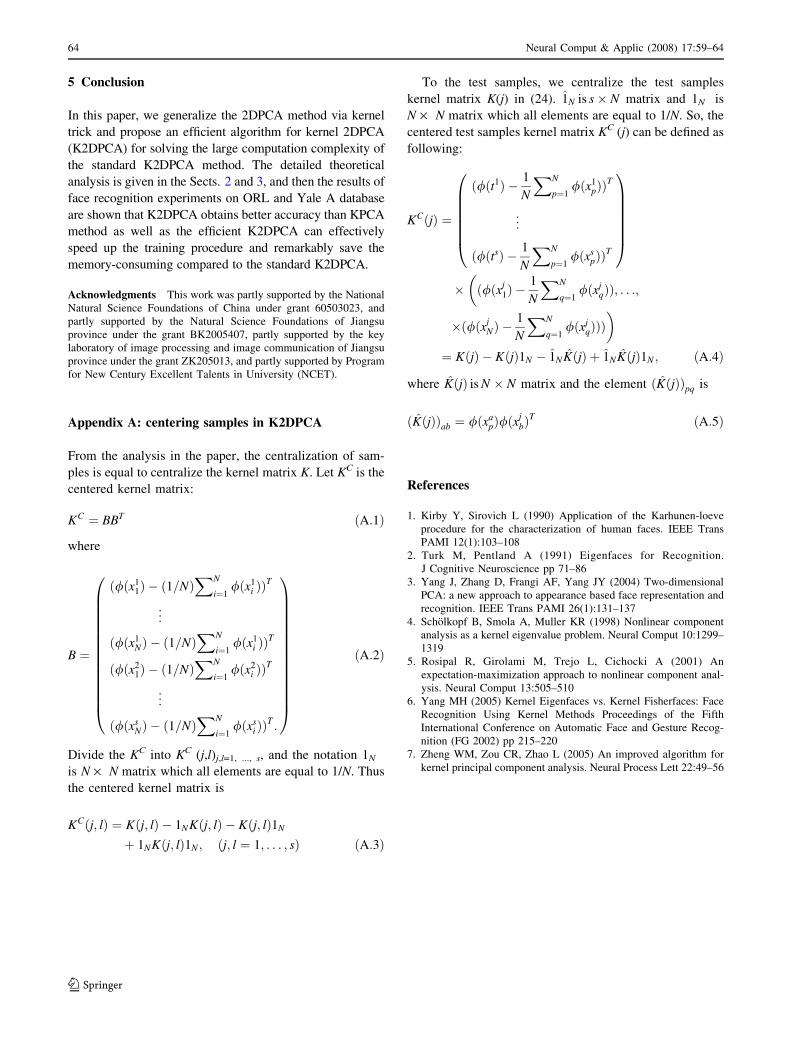
Furthermore, the recognition rate of K2DPCA and

KPCA under different database and different polynomial

kernel degree is sketched in Fig.1, which shows K2DPCA

obtains better accuracy than KPCA method.

Table 4 Comparison of the

training time and space needed

with different samples and

Gaussian kernel on ORL

database

Method Samples 2r2 Dimension Time (s) Space (Mb) Accuracy (%)

Standard K2DPCA 160 5 · 105 4480 · 2044 6340 486 94.58

120 5 · 105 3360 · 178 3,745 361 91.67

80 1 · 105 2240 · 126 2,046 304 84.58

Efficient K2DPCA 160 5 · 105 1774 · 25 800 89 94.17

120 5 · 105 1363 · 25 482 71 91.67

80 1 · 105 925 · 20 253 43 84.17

Table 5 Comparison of the

training time and space needed

with different samples and

polynomial kernel on Yale A

database

Method Samples d Dimension Time (s) Space (Mb) Accuracy (%)

Standard K2DPCA 105 3 3780 · 53 4760 322 94.91

90 2 3240 · 46 2815 245 94.67

75 3 2700 · 36 1890 230 93.33

Efficient K2DPCA 105 3 1272 · 12 585 44 94.91

90 2 980 · 12 225 42 94.67

75 2 860 · 10 162 34 93.33

Table 6 Comparison of the

training time and space needed

with different samples and

Gaussian kernel on Yale A

database

Method Samples 2r2 Dimension Time(s) Space(Mb) Accuracy(%)

Standard K2DPCA 105 5 · 105 3780 · 170 5877 430 96.67

90 5 · 105 3240 · 147 3657 344 96.00

75 5 · 105 2700 · 120 2646 312 94.44

Efficient K2DPCA 105 5 · 105 1511 · 20 760 62 96.67

90 5 · 105 1170 · 20 440 55 96.00

75 5 · 105 954 · 20 280 51 93.33

0 1 2 3 4 5 6 775

80

85

90

95

d−value

Rec

ogni

tion

rate

(%)

K2DPCA on ORL databaseKPCA on ORL databaseK2DPCA on Yale A databaseKPCA on Yale A database

Fig. 1 K2DPCA on ORL database KPCA on ORL database

K2DPCA on Yale A database KPCA on Yale A database

Neural Comput & Applic (2008) 17:59–64 63

123

5 Conclusion

In this paper, we generalize the 2DPCA method via kernel

trick and propose an efficient algorithm for kernel 2DPCA

(K2DPCA) for solving the large computation complexity of

the standard K2DPCA method. The detailed theoretical

analysis is given in the Sects. 2 and 3, and then the results of

face recognition experiments on ORL and Yale A database

are shown that K2DPCA obtains better accuracy than KPCA

method as well as the efficient K2DPCA can effectively

speed up the training procedure and remarkably save the

memory-consuming compared to the standard K2DPCA.

Acknowledgments This work was partly supported by the National

Natural Science Foundations of China under grant 60503023, and

partly supported by the Natural Science Foundations of Jiangsu

province under the grant BK2005407, partly supported by the key

laboratory of image processing and image communication of Jiangsu

province under the grant ZK205013, and partly supported by Program

for New Century Excellent Talents in University (NCET).

Appendix A: centering samples in K2DPCA

From the analysis in the paper, the centralization of sam-

ples is equal to centralize the kernel matrix K. Let KC is the

centered kernel matrix:

KC ¼ BBT ðA:1Þ

where

B ¼

ð/ðx11Þ � ð1=NÞ

XN

i¼1/ðx1

i ÞÞT

..

.

ð/ðx1NÞ � ð1=NÞ

XN

i¼1/ðx1

i ÞÞT

ð/ðx21Þ � ð1=NÞ

XN

i¼1/ðx2

i ÞÞT

..

.

ð/ðxsNÞ � ð1=NÞ

XN

i¼1/ðxs

i ÞÞT :

0

BBBBBBBBBBBBBB@

1

CCCCCCCCCCCCCCA

ðA:2Þ

Divide the KC into KC (j,l)j,l=1, ..., s, and the notation 1N

is N · N matrix which all elements are equal to 1/N. Thus

the centered kernel matrix is

KCðj; lÞ ¼ Kðj; lÞ � 1NKðj; lÞ � Kðj; lÞ1N

þ 1NKðj; lÞ1N ; ðj; l ¼ 1; . . . ; sÞ ðA:3Þ

To the test samples, we centralize the test samples

kernel matrix K(j) in (24). 1N is s� N matrix and 1N is

N · N matrix which all elements are equal to 1/N. So, the

centered test samples kernel matrix KC (j) can be defined as

following:

KCðjÞ ¼

ð/ðt1Þ � 1

N

XN

p¼1/ðx1

pÞÞT

..

.

ð/ðtsÞ � 1

N

XN

p¼1/ðxs

pÞÞT

0BBBBBB@

1CCCCCCA

� ð/ðxj1Þ �

1

N

XN

q¼1/ðxj

qÞÞ; . . .;

�

�ð/ðxjNÞ �

1

N

XN

q¼1/ðxj

qÞÞÞ�

¼ KðjÞ � KðjÞ1N � 1NKðjÞ þ 1NKðjÞ1N ; ðA:4Þ

where KðjÞ is N � N matrix and the element ðKðjÞÞpq is

ðKðjÞÞab ¼ /ðxapÞ/ðx

jbÞ

T ðA:5Þ

References

1. Kirby Y, Sirovich L (1990) Application of the Karhunen-loeve

procedure for the characterization of human faces. IEEE Trans

PAMI 12(1):103–108

2. Turk M, Pentland A (1991) Eigenfaces for Recognition.

J Cognitive Neuroscience pp 71–86

3. Yang J, Zhang D, Frangi AF, Yang JY (2004) Two-dimensional

PCA: a new approach to appearance based face representation and

recognition. IEEE Trans PAMI 26(1):131–137

4. Scholkopf B, Smola A, Muller KR (1998) Nonlinear component

analysis as a kernel eigenvalue problem. Neural Comput 10:1299–

1319

5. Rosipal R, Girolami M, Trejo L, Cichocki A (2001) An

expectation-maximization approach to nonlinear component anal-

ysis. Neural Comput 13:505–510

6. Yang MH (2005) Kernel Eigenfaces vs. Kernel Fisherfaces: Face

Recognition Using Kernel Methods Proceedings of the Fifth

International Conference on Automatic Face and Gesture Recog-

nition (FG 2002) pp 215–220

7. Zheng WM, Zou CR, Zhao L (2005) An improved algorithm for

kernel principal component analysis. Neural Process Lett 22:49–56

64 Neural Comput & Applic (2008) 17:59–64

123