Ann Oper ResDOI 10.1007/s10479-013-1341-4

An effective heuristic for the two-dimensional irregularbin packing problem

Eunice López-Camacho · Gabriela Ochoa ·Hugo Terashima-Marín · Edmund K. Burke

© Springer Science+Business Media New York 2013

Abstract This paper proposes an adaptation, to the two-dimensional irregular bin packingproblem of the Djang and Finch heuristic (DJD), originally designed for the one-dimensionalbin packing problem. In the two-dimensional case, not only is it the case that the piece’ssize is important but its shape also has a significant influence. Therefore, DJD as a selectionheuristic has to be paired with a placement heuristic to completely construct a solution to theunderlying packing problem. A successful adaptation of the DJD requires a routine to reducecomputational costs, which is also proposed and successfully tested in this paper. Results,on a wide variety of instance types with convex polygons, are found to be significantly betterthan those produced by more conventional selection heuristics.

Keywords 2D bin packing problem · Irregular packing · Heuristics · Djang and Finchheuristic

1 Introduction

The problem of finding an arrangement of pieces to cut from or pack inside larger objectsis known as the cutting and packing problem, which is NP-hard. The two-dimensional (2D)bin packing problem (BPP) is a particular case of the basic problem. It consists of finding

E. López-Camacho (�) · H. Terashima-MarínTecnológico de Monterrey, Av. E. Garza Sada 2501, Monterrey, NL, 64849, Mexicoe-mail: eunice.lopez@itesm.mx

H. Terashima-Maríne-mail: terashima@itesm.mx

G. Ochoa · E.K. BurkeComputing Science and Mathematics, University of Stirling, Stirling, Scotland, UK

G. Ochoae-mail: gabriela.ochoa@cs.stir.ac.uk

E.K. Burkee-mail: e.k.burke@stir.ac.uk

Ann Oper Res

an arrangement of pieces inside identical objects such that the number of objects requiredto contain all pieces is minimum. The case of rectangular pieces is the most widely stud-ied. However, the irregular case is seen in a number of industries where parts with irregularshapes are cut from rectangular materials. For example, in the shipbuilding industry, plateparts with free-form shapes for use in the inner frameworks of ships are cut from rectangu-lar steel plates, and in the apparel industry, parts of clothes and shoes are cut from fabric orleather (Okano 2002). Other direct applications include the optimization of layouts withinthe wood, metal, plastics, carbon fiber and glass industries. In these industries, small im-provements of the arrangement can result in a large saving of material (Hu-yao and Yuan-jun2006).

This paper proposes a heuristic for selecting the next pieces to be placed when solving the2D irregular BPP. The proposed heuristic is not only fast in execution, but it also producesexcellent results when compared against more conventional selection heuristics. A simplebut successful placement procedure is also presented, which produces outstanding resultswhen coupled with the proposed selection heuristic. The paper proceeds as follows. Thenext section presents the problem description and a literature review. Section 3 describes theDJD heuristic, which is the base for our approach. Section 4 describes the implementationdetails of the heuristic. Finally, Sects. 5 and 6 give the experimental results and conclusions,respectively.

2 The 2D irregular bin packing problem

The cutting and packing problem is among the earliest problems in the literature of oper-ational research. Wäscher et al. (2007) suggested a complete problem typology which isan extension of Dychoff (1990). In this paper, we consider the problem classified as the2D irregular single bin size bin packing problem in Wäscher, Haussner and Schumann’stypology. Given a set L = (a1, a2, . . . , an) of pieces to cut or pack and an infinite set ofidentical rectangular larger elements (called objects), the problem consists of finding an ar-rangement of pieces inside the objects such that the number of objects required to containall pieces is minimum. A feasible solution is an arrangement of pieces without overlaps andwith no piece outside the object limits. A problem instance or instance I = (L,x0, y0) con-sists of a list of elements L and object dimensions x0 and y0. The term 2D regular BPP ismainly used when all pieces are rectangular (although circles and other regular shapes couldfall under this name too Wäscher et al. 2007); otherwise, the problem is called 2D irregularBPP. The problem is offline, and therefore the list of pieces to be packed is static and givenin advance.

The strip packing problem is a popular variant of the 2D cutting and packing prob-lem which has only one large rectangular object with fixed width, its length is variable andhas to be minimized after placing all the small pieces (some approaches and reviews byDowsland and Dowsland 1995; Hopper and Turton 2001; Burke et al. 2006). A variationof this typical strip packing problem consists on nesting irregular pieces in one large irreg-ular object (examples by Lamousin and Dobson 1996; Lamousin and Waggenspack 1997;Whelan and Batchelor 1992; Ramesh 2001). The amount of research devoted to the strippacking problem has been larger when compared to the research about the 2D irregularBPP. We found that Okano (2002) studied a problem similar to our 2D irregular single binsize BPP but using variable bin sizes, where the problem solution involves finding appro-priate sizes of material objects (bins) among given standard sizes in order to reduce waste.As far as we know, there are no previous studies for, specifically, the 2D irregular single bin

Ann Oper Res

size bin packing problem. Therefore, all 2D irregular problem instances in the literature areintended for the strip packing problem; and there are not 2D irregular BPP instances avail-able. Also, since the strip packing problem is similar to the 2D irregular BPP, many heuristicimplementations may be similar; although, results for both kind of problems are not compa-rable. Nevertheless the lack of research in the 2D irregular BPP, there exist many practicalapplications where irregular pieces are cut from identical rectangular objects (Okano 2002).

For the 1D case, it is common to use the terms items and bins, regarding the small andlarge elements respectively; whereas, for the 2D case, a variety of terms has been used. Thesmall elements have been named pieces, shapes or items; and the large elements have beencalled objects, stock or sheets. Here, we use the terms items and bins regarding the 1D case,and pieces and objects when referring to the 2D case.

For many real-world problems, an exhaustive search for solutions is not a practical propo-sition due to the large size of the solution search space. Hence, many heuristic approacheshave been adopted. It is common that heuristic approaches for the bin packing problempresent at least two phases: first, the selection of the next piece to be placed and the cor-responding object to place it; and second, the actual placement of the selected piece in aposition inside the object according to some given criteria. Some approaches consider athird phase as a local search mechanism.

The placement procedure for irregular pieces has attracted more attention than the explo-ration of the selection criteria. There are several techniques to generate potential placementpositions for the next piece to be placed, and many of them are based on building the no-fitpolygon. The no-fit polygon gives the set of non-overlapping placements for a given pair ofpolygons. Good examples of this type of procedure that work well for the strip packing prob-lem are described by Hu-yao and Yuan-jun (2006), Gomes and Oliveira (2002), Dowslandet al. (2002), Burke and Kendall (1999b), Burke et al. (2007). While the no-fit polygon is apowerful geometric technique, there are several issues that limit its scalability for industrialapplications. No-fit polygon techniques are notorious for the large quantity of degeneratecases that must be handled to make it completely robust (Burke et al. 2006). Whilst thegeneration of the no-fit polygon is academically challenging, it is a tool and not a solution(Burke et al. 2007). After generating the possible placement positions, it is necessary to havesome criteria for choosing the best position. In 2D cutting and packing problems the mostcommonly used method for packing regular and irregular pieces involves the bottom-leftclass of heuristics. These methods involve simply placing the input list of pieces into thebottom-leftmost location on the packing sheet (Allen et al. 2011).

Regarding the selection criteria, most researchers have focused upon exploring differentways of finding good permutation of pieces. Okano (2002) obtains an ordering of pieceswith respect to their areas and the similarities among them. Dowsland et al. (2002) use eightstatic orderings, which have the common strategy of trying to place the difficult-to-placepieces first. Dynamic selection permits all pieces to be available to be placed next Bennelland Oliveira (2009), for example, Bennell and Song (2010) use beam search. This approachsearches the breadth first tree, and prunes the tree at each level according to two evaluationfunctions.

Several metaheuristic approaches have been applied to the strip packing problems, for ex-ample, tabu search (Bennell and Dowsland 2001), evolutionary computation (Bounsaythipand Maouche 1997) and ant algorithms (Burke and Kendall 1999a). Metaheuristic tech-niques are often very effective; however, there can be some reluctance to use them formoney-critical problems. Practitioners in industry often favor the use of very simple andreadily understandable methods even if they deliver relatively inferior results (Ross 2005).Among the main criticisms of stochastic-based problem solving techniques are: (1) the fact

Ann Oper Res

that they involve some randomness and unpredictability, so that identical runs may deliververy different results; (2) there is little understanding about their average- and worst-casebehavior (Ross and Marín-Blázquez 2005); (3) solutions quality greatly depend on a goodparameter choice; and (4) the parameter tunning task requires time, knowledge and ex-perience about the problem domain and properties which makes metaheuristics problem-specific solution methods that can be developed and deployed only by experts (Ross 2005;Bilgin et al. 2006).

3 The DJD heuristic

The proposed approach is based on the DJD heuristic, which is a selection heuristic designedfor the 1D case. In its original version, as explained by Ross et al. (2002), the DJD heuristicputs items into a bin, taking items largest-first until that bin is at least one third full. Itthen tries to find one, or two, or three items that completely fill the bin. If there is no suchcombination it tries again, but looking instead for a combination that fills the bin to within1 unit of its capacity. If that fails, it tries to find a combination that fills the bin to within2 units of its capacity; and so on. This routine is to be performed as long as there are piecesto place. DJD is a single-pass constructive heuristic. A popular variation of DJD is calledDJT (Djang and Finch, more tuples) which considers combinations of up to five items ratherthan three items.

Problems known to be hard have certain characteristics. In bin packing, especially inthe 1D case, instances with many small items are not hard, since the small items can beemployed as sand to fill up the remaining space when large items were packed. Difficultyarises when most of the pieces have an area that is a significant fraction of the total objectarea, for example at least 20 % of the object area, so that the challenge is to find the subsetamong a large number of pieces to be placed in a given object (Ross 2005). We hypothesizethat the DJD heuristic is intended for these kind of hard instances; because, exactly as stated,it works well in many problems known to be hard, but it fails in other types of problem. Forexample, consider a very easy problem in which the bins have capacity 1000 and there are10,000 items each of weight 1. Packing these items will need only 10 bins. However, DJDwill first fill a bin until it contains 334 items (just over one-third) and then add just threemore items into the bin, so the bin will contain 337 items. Thus, 30 bins will be needed(337 × 29 = 9773) (Ross 2005), a solution far from optimality. The obvious remedy to thissituation is to keep trying to place item combinations until no single item can be placed.Although, in the case when items are so small compared with the bin free space, there is noadvantage in trying every combination of items, since no combination would result in zerowaste in the first attempts.

Ross et al. (2002, 2003), Marín-Blázquez and Schulenburg (2006) and Pillay (2012)have implemented the DJD and its variation DJT for the 1D BPP as a part of procedures(hyper-heuristics) that learn to combine heuristics for solving the underlying problem. Inthese approaches, the idea is to automatically apply different heuristics to different states ofthe construction process. In this scenario, DJD and DJT were reported as the best heuris-tics considered. Also, the DJD heuristic was adapted to solve the problem of schedulingtransportation events for minimizing the number of vehicles used, while satisfying the cus-tomer demand (Terashima-Marín et al. 2005b). Kos and Duhovnik (2000) describe the sameheuristic but named it as Exact Fit in an approach for rod cutting optimization with remnantsutilization. Sim et al. (2012) present an evolutionary algorithm for evolving classifiers thatare used for predicting the best heuristic to solve each of a set of unseen 1D BPP instances.

Ann Oper Res

They present the Adaptive DJD which packs items into a bin in descending order until thefree space in the bin is less than or equal to three times the average size of the items re-maining to be packed. This recent version of the DJD heuristic obtains poorer results thanthe DJD and DJT when the metric is the percentage of instances solved using the optimumnumber of bins. When the metric is the fitness given in Eq. (2) or the percentage of extrabins required over the optimal, Adaptive DJD is better than DJD and worse than DJT whenaveraging 1320 instances.

Where pieces to be placed are rectangles, DJD and DJT have been adapted and imple-mented as a selection heuristic (Terashima-Marín et al. 2005a, 2006). For the 2D irregularBPP, where pieces to be placed are convex polygons, DJD has been implemented as a mem-ber of a heuristic repository in a hyper-heuristic approach (Terashima-Marín et al. 2010).To our knowledge, DJT has not been implemented for the 2D irregular BPP. In the previousstudies, the performance of DJD was not analyzed, nor reported separately and the authorsdid not report a routine for improving the running times. This is essential in the 2D case,because simply comparing the area of a 1, 2 or 3-piece combination against the free area ofthe object does not imply that the pieces can actually be placed. Indeed, several groups ofpieces may need to be tried before a given combination of pieces can be placed. Moreover,the same pieces may be tested several times in different combinations before the algorithmis successful in placing a 1, 2 or 3-piece group. Besides, to determine whether or not a piececan be placed in a given object is the most time-consuming task when solving a 2D binpacking problem. The placement task requires even more running time when pieces are ir-regular. In this paper, DJD is adapted to and thoroughly analyzed when solving a variety ofinstances of the 2D irregular BBP. Moreover, a routine for reducing redundant computationis proposed and successfully tested.

4 The proposed DJD heuristic for the 2D irregular BPP

The DJD algorithm for the 2D case works as a selection heuristic, but it alone does notsolve the problem completely. DJD has to be paired with a placement heuristic which willdetermine the exact position of each piece inside an object.

For the 2D case (regular and irregular), the general process of the DJD heuristic is out-lined in the pseudo code of Algorithm 1. In the 2D adaptation of the heuristic, DJD putspieces into an object, taking them by decreasing area, until at least one-third of its area iscovered. It then tries to find one, or two, or three pieces that completely fill the object. Ifthere is no such combination it tries again, but looks instead for a combination that fills thebin to within w of its capacity. If that fails, it tries to find such a combination that fills theobject to within 2w of its capacity; and so on. In the 1D case, the waste incremental sug-gested is 1 unit. Depending on the order of magnitude of the object and pieces sizes, in 2Dit would not be feasible to manage a 1-unit incremental. Therefore, the incremental shouldbe selected according to the total object area. For the 2D adaptation of the heuristic, theprocesses of reviewing groups of one, two or three pieces are modified to optimize runningtime. These processes mentioned in Algorithm 1, are described in Algorithms 2, 3 and 4respectively.

Pieces are placed sequentially when trying groups of 2 or 3 pieces. Only when the firstpiece is placed successfully, a next one is tried, and so on. If all possible second pieces failto fit, the first piece is unplaced and then we try a different group.

Every time a combination of 1, 2 and 3 pieces is placed, the checking process starts allover again in the same object (resetting the allowed waste to 0). Only when no more pieces

Ann Oper Res

Algorithm 1 The DJD heuristicInput: A list of pieces sorted by decreasing area; width and height of the rectangular ob-

jects.Output: All pieces placed in objects.

1: waste = 0; w [increment of allowed waste, w = 1 in the original version of the heuristic]

2: while there are pieces to place do3: Fill the object until at least one-third of its area is covered4: Register in memory every piece that does not fit

5: Try pieces one by one [see Algorithm 2]6: if a piece could be placed leaving a free area up to waste then7: reset waste = 0 and start again trying pieces one by one

8: Try groups of 2 pieces [see Algorithm 3]9: if a pair of pieces could be placed leaving a free area up to waste then

10: reset waste = 0 and start again trying pieces one by one

11: Try groups of 3 pieces [see Algorithm 4]12: if a group of 3 pieces could be placed leaving a free area up to waste then13: reset waste = 0 and start again trying pieces one by one

14: if no piece could be placed trying all possible 1, 2 or 3-piece groupsAND waste < object free area then

15: waste = waste + w

16: else17: open a new object

Algorithm 2 Trying pieces one by one1: for all pieces in decreasing size order do2: if object free area − area of piece > waste then3: break4: if area of piece > object free area OR piece has failed to fit then5: continue [with the next piece]6: Try to place the piece in the object7: if the piece could be placed then8: return9: else

10: register in memory that the piece does not fit

can be placed in an object, a new object is opened. The DJD heuristic works in one openobject at a time, there is no need to review previous open objects. Order is important in 2Dpacking; groups with the same pieces are revised considering all possible orderings. Whenexecuting a placement heuristic, a piece combination that cannot be placed in a particularorder could be placed in another piece order.

In order to reduce the computational effort, a record of what pieces have been tried so faras a first member of a 1, 2 or 3-pieces group is kept for each object, so the algorithm does

Ann Oper Res

Algorithm 3 Trying groups of 2 pieces1: for all pieces in decreasing size order do2: if object free area − piece’s area − largest piece’s area > waste then3: break4: if the piece has failed to fit OR piece’s area + smallest piece’s area > free space then5: continue [with the next piece in the list]6: Try to place the piece in the object7: if piece could not be placed then8: register it in memory9: else {select a second piece when a first piece succeeded to be placed}

10: for all remaining pieces do11: if object free area − area of the 2 pieces > waste then12: break13: if the piece or the pair of pieces has failed to fit OR 2 pieces’ area > free space

then14: continue [with the next piece]15: Try to place the second piece in the object16: if the piece could be placed then17: return18: else19: unplace first piece AND register that the pair of pieces does not fit

not try again the same piece in a different group. Additionally, a record is kept of all orderedpairs of pieces that failed to be placed in a particular object either as a 2-piece group or asthe first 2 pieces of a 3-piece group. These pairs of pieces are, therefore, not tried again inthe same order in the same object. Finally, all ordered 3-piece groups that fail to fit in anobject are recorded as well. These records help to reduce an important amount of redundantcomputation.

As it can be seen in Algorithms 2, 3 and 4, when DJD checks one, two or three-piecegroups, first it compares the pieces’ areas against the maximum waste allowed and againstthe available object area. Only then, does DJD try to place them. For the 2D BPP, checkingif a piece could or could not be placed, is computationally expensive. Pieces should be indescending order when the DJD heuristic starts, allowing the For cycles to break at somepoint when reviewing pieces; thus, reducing comparisons (see Algorithms 2, 3 and 4).

According to the placement procedures considered, when a piece cannot be placed in anobject at a given time, there is a slight possibility that it can actually be placed later when oneor more pieces had been placed. Considering this possibility in the implementation wouldincrease the algorithm running time. If time is not a constraint, the option would be to keepa record of pieces that fail to fit just until one piece or group is placed, and then clean up therecords.

5 Algorithms for geometric computation

The algorithms presented in this section are the building blocks for implementing the place-ment heuristics (Sect. 6.2). These algorithms are suited for dealing with convex and non-convex shapes (even though our testbed instances have only convex pieces). Each piece is

Ann Oper Res

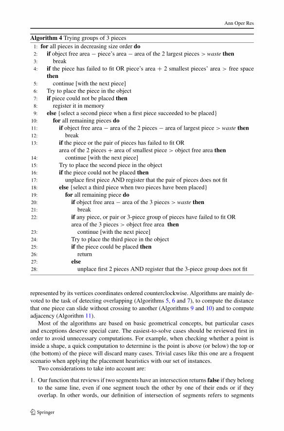
Algorithm 4 Trying groups of 3 pieces1: for all pieces in decreasing size order do2: if object free area − piece’s area − area of the 2 largest pieces > waste then3: break4: if the piece has failed to fit OR piece’s area + 2 smallest pieces’ area > free space

then5: continue [with the next piece]6: Try to place the piece in the object7: if piece could not be placed then8: register it in memory9: else {select a second piece when a first piece succeeded to be placed}

10: for all remaining pieces do11: if object free area − area of the 2 pieces − area of largest piece > waste then12: break13: if the piece or the pair of pieces has failed to fit OR

area of the 2 pieces + area of smallest piece > object free area then14: continue [with the next piece]15: Try to place the second piece in the object16: if the piece could not be placed then17: unplace first piece AND register that the pair of pieces does not fit18: else {select a third piece when two pieces have been placed}19: for all remaining piece do20: if object free area − area of the 3 pieces > waste then21: break22: if any piece, or pair or 3-piece group of pieces have failed to fit OR

area of the 3 pieces > object free area then23: continue [with the next piece]24: Try to place the third piece in the object25: if the piece could be placed then26: return27: else28: unplace first 2 pieces AND register that the 3-piece group does not fit

represented by its vertices coordinates ordered counterclockwise. Algorithms are mainly de-voted to the task of detecting overlapping (Algorithms 5, 6 and 7), to compute the distancethat one piece can slide without crossing to another (Algorithms 9 and 10) and to computeadjacency (Algorithm 11).

Most of the algorithms are based on basic geometrical concepts, but particular casesand exceptions deserve special care. The easiest-to-solve cases should be reviewed first inorder to avoid unnecessary computations. For example, when checking whether a point isinside a shape, a quick computation to determine is the point is above (or below) the top or(the bottom) of the piece will discard many cases. Trivial cases like this one are a frequentscenario when applying the placement heuristics with our set of instances.

Two considerations to take into account are:

1. Our function that reviews if two segments have an intersection returns false if they belongto the same line, even if one segment touch the other by one of their ends or if theyoverlap. In other words, our definition of intersection of segments refers to segments

Ann Oper Res

Algorithm 5 Decide if two pieces intersects each otherInput: A list of coordinates of two pieces P1 and P2.Output: A boolean value indicating whether the two pieces intersects each other.

1: if lowest end of P1 is above upper end of P2 OR lowest end of P2 is above upper end ofP1 then

2: return false3: if leftmost end of P1 is right of the rightmost end of P2 OR leftmost end of P2 is right

of the rightmost end of P1 then4: return false

5: for all edges e1 of P1 do6: for all edges e2 of P2 do7: if Intersects(e1, e2) then8: return true9: return false

Algorithm 6 Decide if a point is inside a shapeInput: A list of coordinates of a piece and a point (x, y).Output: A boolean value indicating whether the point is or not inside the piece.

1: if x ≤ the piece lowest part OR x ≥ the piece upper part then2: return false3: if y ≤ the piece leftmost part OR y ≥ the piece rightmost part then4: return false5: for all vertices of the piece do6: if the point (x, y) is equal to the vertex then7: return false8: for all sides of the piece do9: if the point (x, y) is along the side then

10: return false

11: Create the point (M,y), where M is a very large number.12: for all sides of the piece do13: if the side of the piece intersects the segment (x, y) to (M,y) then14: counter ++15: for all vertices i of the piece do16: if the vertex belong to the segment (x, y) to (M,y) then17: D1 ← Dfunction(segment, vertex i − 1) [see Eq. (1)]18: D2 ← Dfunction(segment, vertex i + 1)19: if D1 and D2 have different signs then20: counter ++

21: if counter is odd then22: return true23: else24: return false

Ann Oper Res

Fig. 1 Ray from point P to theright actually touches 4 times theshape boundaries. The raycrosses the shape at vertex B . Incontrast, the ray touches vertex A

only tangentially and does notcross the shape at this point.Therefore, the count for crossesis 3. Since 3 is an odd number,we conclude that P is inside theshape

Fig. 2 Interpretation of theD-function

that crosses but are not coincident. Note that this definition implies that reviewing forintersection of two segments that are exactly the same, the function will return false.

2. Our function that reviews if a point is inside a segment returns true if the point is one ofthe ends of the segment. When the sum of the distances from the point to the two endsof the segment is equal to the segment length, then we consider that the point belongs tothe segment.

To know whether two pieces intersects each other, a routine that checks intersection foreach pair of sides from both pieces was implemented (Algorithm 5). Initially, a revision isdone to confirm that the orthogonal rectangles that circumscribe both pieces intersect. Thisis used to discard the easiest non-intersection cases. This test does not work if one piece iscompletely inside the other, in which case no edges intersect but the pieces do intersect. Inconsequence, this algorithm is always followed by Algorithm 7 that reviews if one piece iscompletely inside another.

Algorithm 6 determines whether a point is inside a shape. If the point is along an edgeof the piece or one of its vertices, then the algorithm will return false. The basic idea is totrace a ray from the point to any fixed direction. If the ray cuts the shape an odd number oftimes, then the point is inside the shape; otherwise it is outside. If the ray touches a vertexof the shape; it is important to determine if the ray touches the shape tangentially or if itactually crosses the shape (see Fig. 1). This is done employing the D-function (Eq. (1)). Forline intersection, the D-function gives the relative position of a point P with respect to anoriented edge AB (see Fig. 2). The D-function is defined as follows:

DABP = (XA − XB)(YA − YP ) − (YA − YB)(XA − XP ) (1)

Depending if DABP is negative or positive, the point P is on the left or the right side ofthe edge AB . The definition of left and right is as follows: if an observer would stand atpoint A looking in the direction of B , point P would be at the observer’s left or right. IfDABP = 0, the point P is on the supporting line of edge AB (Bennell and Oliveira 2008).

Algorithm 7 is used to determine if a piece is completely inside another piece. Initially,a revision is done to confirm that the orthogonal rectangles that circumscribe both pieces

Ann Oper Res

Algorithm 7 Decide if a shape is completely inside another shapeInput: The two pieces P1 and P2.Output: A boolean value indicating whether one of the pieces is inside the other.

Part 11: if lowest end of P1 is above upper end of P2 OR lowest end of P2 is above upper end of

P1 then2: return false3: if leftmost end of P1 is right of the rightmost end of P2 OR leftmost end of P2 is right

of the rightmost end of P1 then4: return false5: if the 2 pieces intersect each other [see Algorithm 5] then6: return false

Part 2 [At this point we only have pieces that do not intersect each other]7: ymax ← max(maximum P1 y-coordinate, maximum P2 y-coordinate)8: ymin ← min(minimum P1 y-coordinate, minimum P2 y-coordinate)9: xmax ← max(maximum P1 x-coordinate, maximum P2 x-coordinate)

10: xmin ← min(minimum P1 x-coordinate, minimum P2 x-coordinate)11: if (ymax − ymin)(xmax − xmin) <(area of P1+ area of P2) then12: return true

Part 313: y1 ← average(maximum P1 y-coordinate, minimum P1 y-coordinate)14: x1 ← average(maximum P1 x-coordinate, minimum P1 x-coordinate)15: y2 ← average(maximum P2 y-coordinate, minimum P2 y-coordinate)16: x2 ← average(maximum P2 x-coordinate, minimum P2 x-coordinate)17: if point (x1, y1) is inside P1 and P2 or point (x2, y2) is inside P1 and P2 then18: return true

Part 419: for all vertices and edge midpoints and points near each vertex of P1 do20: if inside P2 then21: return true22: for all vertices and edge midpoints and points near each vertex of P2 do23: if inside P1 then24: return true

Part 525: if P1 is equal to P2 and in the same position then26: return true27: else28: return false

intersect and that the actual pieces do not intersect (part 1). If both pieces do not intersect,we find the orthogonal rectangle that circumscribe both pieces at the same time. If the areaof this rectangle is less than the sum of areas of both pieces, it means unequivocally that onepiece is inside the another (part 2). If the point in the middle of piece 1 is inside piece 1, then

Ann Oper Res

Fig. 3 Piece AEFG is inside piece ABCDEFG. In this case, checking if all vertices and edges midpointsof AEFG are inside ABCDEFG will return false. Only when a point very close to vertex E is found insideABCDEFG, the algorithm returns true to the question about if one of the pieces is inside the other. In thiscase, reviewing intersection of these two pieces with Algorithm 5 will return false because none of the sidescrosses another (although they coincide)

Fig. 4 Piece ABCDEFGH contains all area to the (a) left and (b) below a given piece

we check if this point is inside piece 2. The same is checked for the middle point of piece 2(part 3). If this is not the case, then, all vertices and edge midpoints from both pieces arechecked to know if they are inside the other piece. Checking vertices and edges midpoints isnot an infallible test with non-convex shapes. It is possible to find a case where all verticesedges midpoints of the inside shape are all along the contour of the larger piece. See forexample Fig. 3. Therefore, two points close to each vertex (one for each of the edges) arealso tested (part 4). Finally, it is convenient to check whether the two pieces are not equaland in the same position (part 5).

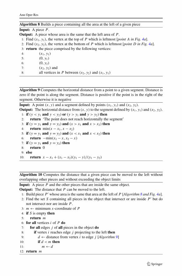
Algorithm 8 builds a piece that holds all the area in the object that is left of a given piece(see Fig. 4a). A similar procedure is done to build a piece containing all the area below agiven piece (see Fig. 4b). Algorithm 9 computes the distance by which a point can reachhorizontally a segment. An analogous procedure finds a vertical distance from a point to agiven segment.

Algorithms 8 and 9 are needed when executing Algorithm 10 which computes the dis-tance that a given piece can be moved to the left avoiding collision against other pieces inthe object and without exceeding the object limits. A similar procedure was implemented inthis investigation to find how much a given piece can be moved down. The implementationof this algorithm is basic for bottom-left moves that take place in all placement heuristics(Sect. 6.2).

Algorithm 11 returns the distance in which two segments coincide. This algorithm consti-tutes the basis for implementing the heuristic called Constructive Approach with MaximumAdjacency (Sect. 6.2).

Ann Oper Res

Algorithm 8 Builds a piece containing all the area at the left of a given pieceInput: A piece P .Output: A piece whose area is the same that the left area of P .

1: Find (x1, y1), the vertex at the top of P which is leftmost [point A in Fig. 4a].2: Find (x2, y2), the vertex at the bottom of P which is leftmost [point D in Fig. 4a].3: return the piece comprised by the following vertices:4: (x1, y1)

5: (0, y1)

6: (0, y2)

7: (x2, y2) and8: all vertices in P between (x2, y2) and (x1, y1)

Algorithm 9 Computes the horizontal distance from a point to a given segment. Distance iszero if the point is along the segment. Distance is positive if the point is in the right of thesegment. Otherwise it is negativeInput: A point (x, y) and a segment defined by points (x1, y1) and (x2, y2).Output: The horizontal distance from (x, y) to the segment defined by (x1, y1) and (x2, y2).

1: if (y < y1 and y < y2) or (y > y1 and y > y2) then2: return ‘The point does not reach horizontally the segment’3: if (y = y1 and y = y2) and (x > x1 and x > x2) then4: return min(x − x1, x − x2)

5: if (y = y1 and y = y2) and (x < x1 and x < x2) then6: return −min(x1 − x, x2 − x)

7: if (y = y1 and y = y2) then8: return 09: else

10: return x − x1 + (x1 − x2)(y1 − y)/(y1 − y2)

Algorithm 10 Computes the distance that a given piece can be moved to the left withoutoverlapping other pieces and without exceeding the object limitsInput: A piece P and the other pieces that are inside the same object.Output: The distance that P can be moved to the left.

1: Build piece P ′ whose area is the same that area at the left of P [Algorithm 8 and Fig. 4a].2: Find the set S containing all pieces in the object that intersect or are inside P ′ but do

not intersect nor are inside P .3: m ← minimum x-coordinate of P

4: if S is empty then5: return m

6: for all vertices i of P do7: for all edges j of all pieces in the object do8: if vertex i reaches edge j projecting to the left then9: d ← distance from vertex i to edge j [Algorithm 9]

10: if d < m then11: m ← d

12: return m

Ann Oper Res

Algorithm 11 Measures the distance in which two segments coincideInput: The two finite segments S1 and S2.Output: The distance in which S1 and S2 coincide.

1: if lowest end of S1 is above upper end of S2 OR lowest end of S2 is above upper end ofS1 then

2: return 03: if leftmost end of S1 is right of the rightmost end of S2 OR leftmost end of S2 is right of

the rightmost end of S1 then4: return 05: if slope of S1 �= slope of S2 then6: return 07: if y-intercept of S1 �= y-intercept of S2 then8: return 0 [segments are parallel]9: if S1 and S2 are both horizontal then

10: p1 ← rightmost point out of the leftmost ends of S1 and S2.11: p2 ← leftmost point out of the rightmost ends of S1 and S2.12: return distance from p1 to p2

13: else14: p1 ← upper point out of the lowest ends of S1 and S2.15: p2 ← lowest point out of the upper ends of S1 and S2.16: return distance from p1 to p2

6 Experiments and results

This section describes how the DJD is tested against seven other selection heuristics com-bined with four different placement heuristics. Characteristics of the problem instances aregiven as well as a way to measure the quality of the solution.

6.1 The other selection heuristics

The selection heuristics used for comparison against DJD are:

1. First Fit (FF). Considers the open objects in the order they were initially opened, andplaces the next piece in the first object where it fits. If the piece does not fit in any openobject, a new object is opened to place it. Pieces are processed in the order they arepresented in the instance being solved. This heuristic considers all partially filled objectsas candidates for the next piece to be packed.

2. First Fit Decreasing (FFD). Sorts pieces by decreasing area, and places the pieces ac-cording to FF.

3. First Fit Increasing (FFI). Sorts pieces by increasing area, and places the pieces accord-ing to FF.

4. Filler. Sorts the pieces in order of decreasing area and packs as many pieces as possiblewithin the open object. When no single piece can be placed in the open object, a newobject is opened to continue packing the pieces from largest to smallest. This heuristicworks with one open object at a time.

5. Best Fit (BF). Considers the open objects in the increasing order of free area, and placesthe next piece in the first object where it fits, that is, in the object that leaves minimumwaste. If the piece does not fit in any open object, a new object is opened to place it.

Ann Oper Res

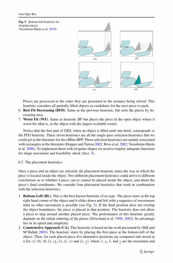
Fig. 5 Bottom-left heuristic forirregular pieces(Terashima-Marín et al. 2010)

Pieces are processed in the order they are presented in the instance being solved. Thisheuristic considers all partially filled objects as candidates for the next piece to pack.

6. Best Fit Decreasing (BFD). Same as the previous heuristic, but sorts the pieces by de-creasing area.

7. Worst Fit (WF). Same as heuristic BF but places the piece in the open object where itworst fits (that is, in the object with the largest available room).

Notice that the first part of DJD, when an object is filled until one-third, corresponds tothe FFD heuristic. These seven heuristics are all the single-pass selection heuristics that wecould get in the literature for the offline BPP. These selection heuristics are mainly associatedwith rectangles in the literature (Hopper and Turton 2002; Ross et al. 2002; Terashima-Marínet al. 2006). To implement them with irregular shapes we need to employ adequate functionsfor shape movement and feasibility check (Sect. 5).

6.2 The placement heuristics

Once a piece and an object are selected, the placement heuristic states the way in which thepiece is located inside the object. Two different placement heuristics could arrive to differentconclusions as to whether a piece can or cannot be placed inside the object, and about thepiece’s final coordinates. We consider four placement heuristics that work in combinationwith the selection heuristics:

1. Bottom-Left (BL). This is the best known heuristic of its type. The piece starts at the topright hand corner of the object and it slides down and left with a sequence of movementsuntil no other movement is possible (see Fig. 5). If the final position does not overlapthe object boundaries, the piece is placed in that position. The heuristic does not allowa piece to skip around another placed piece. The performance of this heuristic greatlydepends on the initial ordering of the pieces (Dowsland et al. 1998, 2002). Its advantagelies in its speed and simplicity.

2. Constructive Approach (CA). This heuristic is based on the work presented by (Hifi andM’Hallah 2003). The heuristic starts by placing the first piece at the bottom-left of theobject. Then, for each placed piece five alternative positions are computed and stored ina list: (x,0), (0, y), (x, y), (x, y) and (x, y), where x, x, y, and y are the maximum and

Ann Oper Res

Fig. 6 Positions to beconsidered in the ConstructiveApproach (Terashima-Marínet al. 2010)

Fig. 7 Constructive ApproachHeuristic (Terashima-Marín et al.2010)

minimum coordinates in x and y (see Fig. 6). Given that some positions might coincide,each position appears only once in the list. In our implementation, the four corners of theobject (the large sheet of stock material) were also added as candidate positions. Fromeach position in the list, the next piece slides vertically and horizontally following downand left movements as shown in Fig. 7. Positions with overlapping pieces, or exceedingthe object dimensions, are discarded. Among the remaining positions, the most bottom-left position is chosen. Using the corners as a departure point to slide the piece bottomand left, allows the method to reach certain gaps between pieces, which would not bereachable if only the five initial positions were considered.

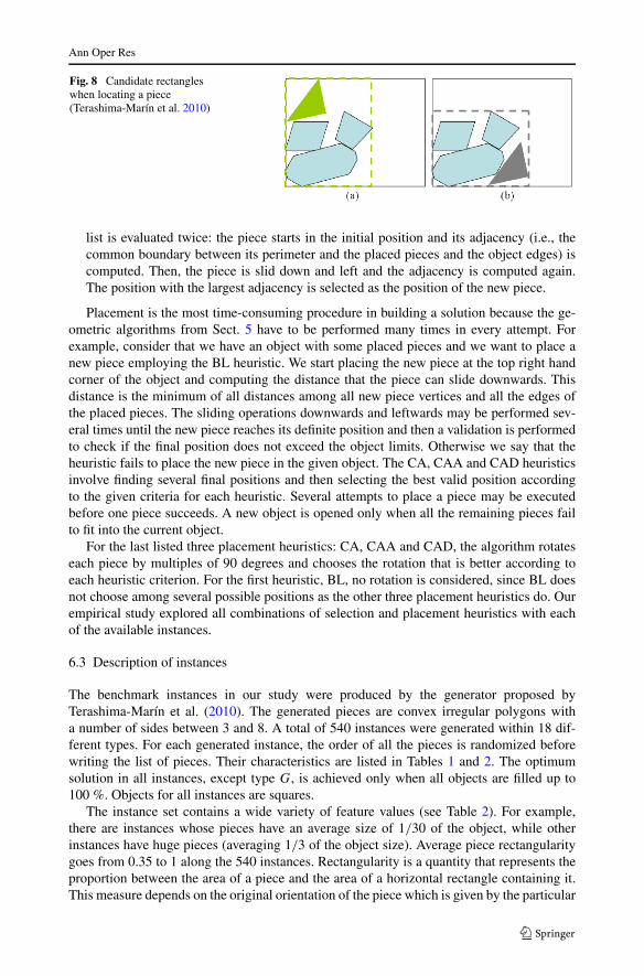
3. Constructive Approach (Minimum Area) (CAA). This is a modification of the previ-ous heuristic. The variation consists of selecting the best position from the list based onwhich one yields the bounding rectangle with minimum area, containing all pieces, andthat fits in the bottom left hand corner of the object. The bounding rectangle area is com-puted with the product of the maximum horizontal coordinate and the maximum verticalcoordinate of all pieces already placed plus the new piece to be located in the proposedposition. Figure 8 shows the rectangle with minimum area for two different positions fora single piece. This criterion was chosen based on the idea of selecting a point with whichall pieces, not only the last piece, are deepest (bottom and left).

4. Constructive Approach (Maximum Adjacency) (CAD). This heuristic is partiallybased on the approach suggested by Uday et al. (2001). However, when the first piece isto be placed, our implementation considers only the four corners of the object. For thesubsequent pieces, the possible points are the same as those in the constructive approach(CA, listed as our second placement heuristic), described above. Each position in the

Ann Oper Res

Fig. 8 Candidate rectangleswhen locating a piece(Terashima-Marín et al. 2010)

list is evaluated twice: the piece starts in the initial position and its adjacency (i.e., thecommon boundary between its perimeter and the placed pieces and the object edges) iscomputed. Then, the piece is slid down and left and the adjacency is computed again.The position with the largest adjacency is selected as the position of the new piece.

Placement is the most time-consuming procedure in building a solution because the ge-ometric algorithms from Sect. 5 have to be performed many times in every attempt. Forexample, consider that we have an object with some placed pieces and we want to place anew piece employing the BL heuristic. We start placing the new piece at the top right handcorner of the object and computing the distance that the piece can slide downwards. Thisdistance is the minimum of all distances among all new piece vertices and all the edges ofthe placed pieces. The sliding operations downwards and leftwards may be performed sev-eral times until the new piece reaches its definite position and then a validation is performedto check if the final position does not exceed the object limits. Otherwise we say that theheuristic fails to place the new piece in the given object. The CA, CAA and CAD heuristicsinvolve finding several final positions and then selecting the best valid position accordingto the given criteria for each heuristic. Several attempts to place a piece may be executedbefore one piece succeeds. A new object is opened only when all the remaining pieces failto fit into the current object.

For the last listed three placement heuristics: CA, CAA and CAD, the algorithm rotateseach piece by multiples of 90 degrees and chooses the rotation that is better according toeach heuristic criterion. For the first heuristic, BL, no rotation is considered, since BL doesnot choose among several possible positions as the other three placement heuristics do. Ourempirical study explored all combinations of selection and placement heuristics with eachof the available instances.

6.3 Description of instances

The benchmark instances in our study were produced by the generator proposed byTerashima-Marín et al. (2010). The generated pieces are convex irregular polygons witha number of sides between 3 and 8. A total of 540 instances were generated within 18 dif-ferent types. For each generated instance, the order of all the pieces is randomized beforewriting the list of pieces. Their characteristics are listed in Tables 1 and 2. The optimumsolution in all instances, except type G, is achieved only when all objects are filled up to100 %. Objects for all instances are squares.

The instance set contains a wide variety of feature values (see Table 2). For example,there are instances whose pieces have an average size of 1/30 of the object, while otherinstances have huge pieces (averaging 1/3 of the object size). Average piece rectangularitygoes from 0.35 to 1 along the 540 instances. Rectangularity is a quantity that represents theproportion between the area of a piece and the area of a horizontal rectangle containing it.This measure depends on the original orientation of the piece which is given by the particular

Ann Oper Res

Table 1 Description of problem instances

Type Objectsside

Pieces Num. ofinstances

Optimal(num. of objects)

A 1000 30 30 3

B 1000 30 30 10

C 1000 36 30 6

D 1000 60 30 3

E 1000 60 30 3

F 1000 30 30 2

G 1000 36 30 ≤ 15

H 1000 36 30 12

I 1000 60 30 3

J 1000 60 30 4

K 1000 54 30 6

L 1000 30 30 3

M 1000 40 30 5

N 1000 60 30 2

O 1000 28 30 7

P 1000 56 30 8

Q 1000 60 30 15

R 1000 54 30 9

Total 540

instance to solve. The lower the rectangularity, the more irregular the pieces are. As one cansee in Table 2, instances of type I have a rectangularity value of 1 which means that all ofthese instances are rectangular.

6.4 Measure of performance

The quality of a solution, produced by any pair of selection and placement heuristics for agiven instance, is based on the percentage of usage for each object, given by:

f =∑No

i=1 U 2i

No

(2)

where No is the total number of objects used and Ui is the fractional utilization for eachobject i. This measure of fitness rewards objects that are filled completely or nearly so, andavoids the problem of too many ties among different heuristics that occur when performanceis measured by the number of objects used.

6.5 Results

The value of the waste incremental w is an important choice in the DJD heuristic. As ob-served experimentally in our instance set, if the waste incremental is set to w = 1, many1-unit increments occur during the solution construction at a high computational cost with-out placing any single piece. We empirically found that a waste incremental of one-twentiethof the total object area is a good balance between fast and good solutions. Increments lower

Ann Oper Res

Table 2 Characteristics of problem instances

Averagepiecearea

Piece areastandarddeviation

Averagerectan-gularity

Percentageof rightangles

Percentage ofvertical/horizontalsides

Minimum 0.033 0.014 0.35 11 34

Total average 0.154 0.100 0.68 42 65

Maximum 0.354 0.280 1 100 100

Average of instances per type

A 0.100 0.069 0.70 42 68

B 0.333 0.162 0.87 67 84

C 0.167 0.124 0.68 36 63

D 0.050 0.036 0.57 23 51

E 0.050 0.035 0.41 12 38

F 0.067 0.050 0.59 29 57

G 0.332 0.156 0.87 67 83

H 0.333 0.158 0.86 67 83

I 0.053 0.017 1 100 100

J 0.067 0.034 0.83 68 83

K 0.154 0.150 0.63 34 60

L 0.100 0.075 0.51 23 50

M 0.125 0.102 0.55 28 55

N 0.033 0.024 0.62 32 60

O 0.250 0.223 0.57 27 58

P 0.143 0.173 0.49 18 43

Q 0.250 0.053 0.89 51 76

R 0.167 0.153 0.63 36 62

than w = 1/20 of the object total size have a high computational cost, without a significantimprovement in fitness, while increments higher than w = 1/20 of the object size lead toinferior results.

We explored the phenomenon of a piece that cannot fit into an object and it later fits (whenthere are one or more pieces in the object). This is rare for placement heuristics CA, CAAand CAD. Therefore, in this case, trying to fit pieces after they have failed to be placed,increases the running time. Results may be slightly better (or worse) in some cases, butgenerally speaking, the small improvement does not pay the huge excess of processing time(although this would depend on the particular application). For the BL placement heuristicthis phenomenon is less rare. Hence, when using BL in combination with any selectionheuristics, a record of pieces that fail to be placed is kept until a piece is successfully placed.After that, the records are cleaned.

We explored four different initial levels of fullness before trying to place combinationsof pieces within an allowed waste, namely, 1/4, 1/3, 1/2 and 2/3. DJD heuristics with theselevels are referred to as DJD1/4, DJD1/3, DJD1/2 and DJD2/3, respectively. Along with the 7selection heuristics described above, we have 11 different selection heuristics overall.

All instances were solved with all heuristics (11 selection heuristics × 4 placementheuristics = 44 ways to solve a given instance). Figure 9 shows the solution of an instancetype C with the selection heuristic DJD1/3 and the placement heuristic CAD.

Ann Oper Res

Fig. 9 DJD1/3 in combinationwith CAD heuristic solves aninstance of type C. This solutiongets one more object than theoptimal solution in which therewould be zero waste. In thissolution, fitness is 0.776measured with Eq. (2)

Table 3 Average fitness for all the combinations of selection and placement heuristics over the 540 instances

Selection heuristics

Placementheuristics

FF FFD FFI Filler BF BFD WF DJD DJD DJD DJD Average1/4 1/3 1/2 2/3

BL 0.347 0.422 0.302 0.426 0.348 0.423 0.306 0.485 0.472 0.435 0.429 0.400

CA 0.439 0.563 0.352 0.569 0.437 0.564 0.385 0.583 0.583 0.566 0.563 0.510

CAA 0.436 0.560 0.350 0.567 0.438 0.562 0.373 0.574 0.576 0.561 0.562 0.505

CAD 0.501 0.648 0.383 0.650 0.501 0.650 0.421 0.682 0.683 0.653 0.649 0.584

Average 0.431 0.548 0.347 0.553 0.431 0.550 0.371 0.581 0.578 0.554 0.551 0.500

Table 3 shows the average fitness for every possible combination of selection and place-ment heuristics along the 540 instances. Two variants of the DJD heuristic, DJD1/3 andDJD1/4, outperformed the other selection heuristics tried. The best combination of selectionand placement heuristic is DJD1/3 + CAD, closely followed by DJD1/4 + CAD. The place-ment heuristic CAD is clearly the best regardless of which selection heuristic it is pairedwith. For the different variations of the DJD tried, DJD1/4 is the best when used along withthe BL and CA placement heuristics and DJD1/3 is the best when used along with the CA,CAA and CAD placement heuristics. Therefore, we found that the one-third of the objectcapacity for the initial fullness before trying different combinations of pieces, as stated bythe original version of the DJD for 1D BPP, is also suitable for the 2D irregular BPP.

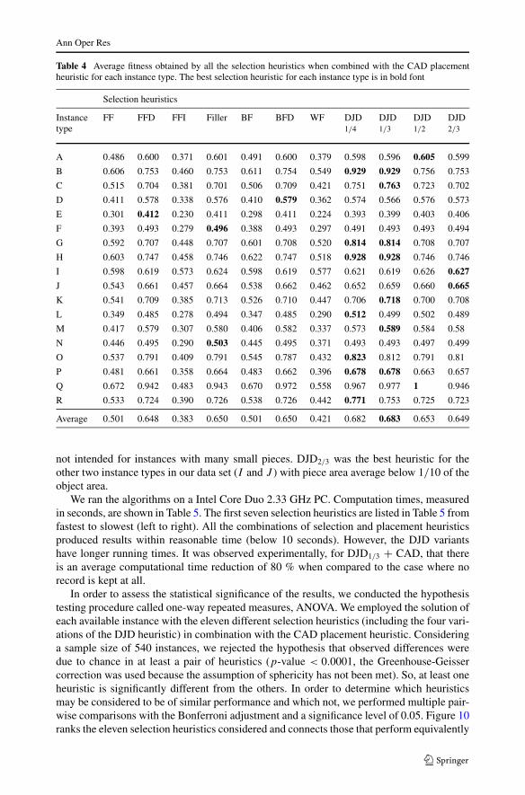
For all the problem instances types from A to R, the CAD heuristic produced better aver-age performance when combined with all the selection heuristics. Table 4 shows the averagefitness obtained by all the selection heuristics with the CAD placement heuristic. Resultsare reported for the CAD placement heuristic only as it produced the best performance.Type I and J are the only instance types where DJD2/3 outperformed all others, and type I

instances are the only ones where all pieces are regular (rectangles). Apart from type I ,type J instances have the highest percentage of right angles. It seems that DJD2/3 goes wellalong with rectangles. All type Q instances are solved to optimally by DJD1/2 using CADplacement heuristic, and 73 % of Q instances were solved to optimally by DJD1/3 + CAD.Optimum solutions of all type Q instances have exactly four pieces in each of 15 objects.Several instances of types B , H and O are also solved to optimally by several variations ofDJD.

Table 4 shows that only four instance types (D, E, F and N ) where solved better for aheuristic different from DJD. These four instance types have an average of piece area belowone-tenth of the object area. As we hypothesized above, it seems that the DJD heuristic is

Ann Oper Res

Table 4 Average fitness obtained by all the selection heuristics when combined with the CAD placementheuristic for each instance type. The best selection heuristic for each instance type is in bold font

Selection heuristics

Instancetype

FF FFD FFI Filler BF BFD WF DJD DJD DJD DJD1/4 1/3 1/2 2/3

A 0.486 0.600 0.371 0.601 0.491 0.600 0.379 0.598 0.596 0.605 0.599

B 0.606 0.753 0.460 0.753 0.611 0.754 0.549 0.929 0.929 0.756 0.753

C 0.515 0.704 0.381 0.701 0.506 0.709 0.421 0.751 0.763 0.723 0.702

D 0.411 0.578 0.338 0.576 0.410 0.579 0.362 0.574 0.566 0.576 0.573

E 0.301 0.412 0.230 0.411 0.298 0.411 0.224 0.393 0.399 0.403 0.406

F 0.393 0.493 0.279 0.496 0.388 0.493 0.297 0.491 0.493 0.493 0.494

G 0.592 0.707 0.448 0.707 0.601 0.708 0.520 0.814 0.814 0.708 0.707

H 0.603 0.747 0.458 0.746 0.622 0.747 0.518 0.928 0.928 0.746 0.746

I 0.598 0.619 0.573 0.624 0.598 0.619 0.577 0.621 0.619 0.626 0.627

J 0.543 0.661 0.457 0.664 0.538 0.662 0.462 0.652 0.659 0.660 0.665

K 0.541 0.709 0.385 0.713 0.526 0.710 0.447 0.706 0.718 0.700 0.708

L 0.349 0.485 0.278 0.494 0.347 0.485 0.290 0.512 0.499 0.502 0.489

M 0.417 0.579 0.307 0.580 0.406 0.582 0.337 0.573 0.589 0.584 0.58

N 0.446 0.495 0.290 0.503 0.445 0.495 0.371 0.493 0.493 0.497 0.499

O 0.537 0.791 0.409 0.791 0.545 0.787 0.432 0.823 0.812 0.791 0.81

P 0.481 0.661 0.358 0.664 0.483 0.662 0.396 0.678 0.678 0.663 0.657

Q 0.672 0.942 0.483 0.943 0.670 0.972 0.558 0.967 0.977 1 0.946

R 0.533 0.724 0.390 0.726 0.538 0.726 0.442 0.771 0.753 0.725 0.723

Average 0.501 0.648 0.383 0.650 0.501 0.650 0.421 0.682 0.683 0.653 0.649

not intended for instances with many small pieces. DJD2/3 was the best heuristic for theother two instance types in our data set (I and J ) with piece area average below 1/10 of theobject area.

We ran the algorithms on a Intel Core Duo 2.33 GHz PC. Computation times, measuredin seconds, are shown in Table 5. The first seven selection heuristics are listed in Table 5 fromfastest to slowest (left to right). All the combinations of selection and placement heuristicsproduced results within reasonable time (below 10 seconds). However, the DJD variantshave longer running times. It was observed experimentally, for DJD1/3 + CAD, that thereis an average computational time reduction of 80 % when compared to the case where norecord is kept at all.

In order to assess the statistical significance of the results, we conducted the hypothesistesting procedure called one-way repeated measures, ANOVA. We employed the solution ofeach available instance with the eleven different selection heuristics (including the four vari-ations of the DJD heuristic) in combination with the CAD placement heuristic. Consideringa sample size of 540 instances, we rejected the hypothesis that observed differences weredue to chance in at least a pair of heuristics (p-value < 0.0001, the Greenhouse-Geissercorrection was used because the assumption of sphericity has not been met). So, at least oneheuristic is significantly different from the others. In order to determine which heuristicsmay be considered to be of similar performance and which not, we performed multiple pair-wise comparisons with the Bonferroni adjustment and a significance level of 0.05. Figure 10ranks the eleven selection heuristics considered and connects those that perform equivalently

Ann Oper Res

Table 5 Average computational time (in seconds) for all the combinations of selection and placement heuris-tics over the 540 instances

Selection heuristics

Placementheuristics

WF BF FF FFI FFD BFD Filler DJD DJD DJD DJD Average1/4 1/3 1/2 2/3

BL 0.01 0.02 0.01 0.02 0.02 0.02 0.04 1.12 0.93 0.68 0.32 0.29

CA 0.41 0.76 0.83 0.85 1.20 1.18 5.77 10.04 9.72 7.83 6.61 4.11

CAA 0.44 0.81 0.80 0.86 1.12 1.22 5.45 9.89 9.54 7.89 6.62 4.06

CAD 0.47 0.95 0.94 0.90 1.33 1.42 6.18 12.52 12.37 10.4 9.02 5.14

Average 0.33 0.63 0.64 0.66 0.92 0.96 4.36 8.40 8.14 6.70 5.64 3.40

Fig. 10 Comparison of means for the 11 heuristics considered, using the Bonferroni adjustment. DJD1/4and DJD1/3 are the better heuristics and there is not significant difference between them

according to the Bonferroni procedure. The FFI heuristic produced the overall lowest fitness,and it is significantly different from the other heuristics. From lowest to highest fitness, thenext heuristic is WF; then, BF and FF form a group of similar heuristics since their fitness isnot significantly different. Two variations of the DJD heuristic (DJD2/3 and DJD1/2) alongwith FFD, Filler and BFD perform in a similar way along the set of considered instances.The heuristics DJD1/4 and DJD1/3 are the best, and are significantly different from the rest.Although DJD1/3 performs slightly better than DJD1/4, this difference is not statisticallysignificant.

7 Conclusions

This article proposed an adaptation, to the two-dimensional irregular bin packing problem,of the Djang and Finch heuristic originally designed for the one-dimensional bin packingproblem. Four variants of the DJD heuristic (with initial fullness of 1/4, 1/3, 1/2 and 2/3,before combinations of pieces are tried to be placed within an allowed waste) were exploredand compared with several alternative selection heuristics in the literature. Selection heuris-tics need to be paired with a placement heuristic to completely solve packing problems.Several placement heuristics were explored and the Constructive Approach with MaximumAdjacency (CAD) was found to outperform the others in our study. Also, the value of thewaste incremental is an important choice in the DJD heuristic. We found, empirically, thata waste incremental of one-twentieth of the total object area represents a good balance be-tween fast and good solutions.

Ann Oper Res

An extensive empirical study was conducted over 540 irregular convex instances of dif-ferent types and a wide range of characteristics. The proposed DJD heuristic was foundto statistically outperform the alternative selection heuristics. Moreover, the computationaltime, although longer for the DJD variants is still within reasonable bounds, which wasachieved by a routine keeping appropriate records to reduce the amount of redundant com-putation. The DJD variants with 1/4 and 1/3 initial fullness levels produced the best results.Therefore, the one-third of the object capacity for the initial fullness before trying differentcombinations of pieces, as stated by the original version of the DJD for the one-dimensionalcase, is also suitable in two dimensions. For further research, we plan to test this adaptationin instances with concave polygons which will increase the level of geometrical complexity.

Acknowledgements This research was supported in part by Instituto Tecnológico y de Estudios Superioresde Monterrey (ITESM) under the Research Chair CAT-144 and the Consejo Nacional de Ciencia y Tecnología(CONACYT) Project under grant 99695. Gabriela Ochoa gratefully acknowledges the British Engineeringand Physical Sciences Research Council (EPSRC) for financial support under grant number EP/D061571/1.

References

Allen, S. D., Burke, E. K., & Kendall, G. (2011). A hybrid placement strategy for the three-dimensionalstrip packing problem. European Journal of Operational Research, 209(3), 219–227. doi:10.1016/j.ejor.2010.09.023.

Bennell, J. A., & Dowsland, K. A. (2001). Hybridising tabu search with optimisation techniques for irregularstock cutting. Management Science, 47(8), 1160–1172.

Bennell, J. A., & Oliveira, J. F. (2008). The geometry of nesting problems: a tutorial. European Journal ofOperational Research, 184(2), 397–415.

Bennell, J. A., & Oliveira, J. F. (2009). A tutorial in irregular shape packing problems. Journal of the Opera-tional Research Society, 60(S1), S93–S105.

Bennell, J. A., & Song, X. (2010). A beam search implementation for the irregular shape packing problem.Journal of Heuristics, 16(2), 167–188.

Bilgin, B., Özcan, E., & Korkmaz, E. E. (2006). An experimental study on hyper-heuristics and examtimetabling. In Proceedings of the 6th international conference on practice and theory of automatedtimetabling (pp. 123–140).

Bounsaythip, C., & Maouche, S. (1997). Irregular shape nesting and placing with evolutionary approach. InIEEE international conference on systems, man and cybernetics (Vol. 4, pp. 3425–3430).

Burke, E. K., & Kendall, G. (1999a). Applying ant algorithms and the no fit polygon to the nesting problem.In Australian joint conference on artificial intelligence (pp. 453–464). London: Springer.

Burke, E. K., & Kendall, G. (1999b). Implementation and performance improvement of the evaluation of atwo dimensional bin packing problem using the no fit polygon (Tech. Rep.). University of Nottingham.Report ASAP99001.

Burke, E. K., Hellier, R. S. R., Kendall, G., & Whitwell, G. (2006). A new bottom-left-fill heuristic algorithmfor the two-dimensional irregular packing problem. Operations Research, 54(3), 587–601.

Burke, E. K., Hellier, R. S. R., Kendall, G., & Whitwell, G. (2007). Complete and robust no-fit polygongeneration for the irregular stock cutting problem. European Journal of Operational Research, 179(1),27–49.

Dowsland, K. A., & Dowsland, W. B. (1995). Solution approaches to irregular nesting problems. EuropeanJournal of Operational Research, 84, 506–521.

Dowsland, K. A., Dowsland, W. B., & Bennell, J. A. (1998). Jostling for position: local improvement forirregular cutting patterns. Journal of the Operational Research Society, 49(6), 647–658.

Dowsland, K. A., Vaid, S., & Dowsland, W. B. (2002). An algorithm for polygon placement using a bottom-left strategy. European Journal of Operational Research, 141(2), 371–381.

Dychoff, H. (1990). A typology of cutting and packing problems. European Journal of Operational Research,44, 145–159.

Gomes, A. M., & Oliveira, J. F. (2002). A 2-exchange heuristic for nesting problems. European Journal ofOperational Research, 141, 359–370.

Hifi, M., & M’Hallah, R. (2003). A hybrid algorithm for the two-dimensional layout problem: the cases ofregular and irregular shapes. International Transactions in Operational Research, 10, 195–216.

Ann Oper Res

Hopper, E., & Turton, B. C. H. (2001). A review of the application of meta-heuristic algorithms to 2D strippacking problems. Artificial Intelligence Review, 16(4), 257–300. doi:10.1023/A:1012590107280.

Hopper, E., & Turton, B. C. H. (2002). An empirical study of meta-heuristics applied to 2D rectangular binpacking—part II. Studia Informatica Universalis, 2(1), 93–106.

Hu-yao, L., & Yuan-jun, H. (2006). NFP-based nesting algorithm for irregular shapes. In Symposium onapplied computing (pp. 963–967). New York: ACM.

Kos, L., & Duhovnik, J. (2000). Rod cutting optimization with store utilization. In International design con-ference, Dubrovnik, Croatia (pp. 313–318).

Lamousin, H., & Waggenspack, J. (1997). Nesting of two-dimensional irregular parts using a shape reasoningheuristic. Computer-Aided Design, 29(3), 221–238. doi:10.1016/S0010-4485(96)00065-6.

Lamousin Jr., H. J., & Dobson, G. T. (1996). Nesting of complex 2-D parts within irregular boundaries.Journal of Manufacturing Science and Engineering, 118(4), 615–622. doi:10.1115/1.2831075.

Marín-Blázquez, J. G., & Schulenburg, S. (2006). Multi-step environment learning classifier systems appliedto hyper-heuristics. In Lecture notes in computer science. Conference on genetic and evolutionary com-putation (pp. 1521–1528). New York: ACM.

Okano, H. (2002). A scanline-based algorithm for the 2D free-form bin packing problem. Journal of theOperations Research Society of Japan, 45(2), 145–161.

Pillay, N. (2012). A study of evolutionary algorithm selection hyper-heuristics for the one-dimensional bin-packing problem. South African Computer Journal, 48, 31–40.

Ramesh, R. (2001). A generic approach for nesting of 2-D parts in 2-D sheets using genetic and heuristicalgorithms. Computer-Aided Design, 33(12), 879–891. doi:10.1016/S0010-4485(00)00112-3.

Ross, P. (2005). Hyper-heuristics. In E. K. Burke & G. Kendall (Eds.), Search methodologies: introductorytutorials in optimization and decision support techniques (pp. 529–556). New York: Springer.

Ross, P., & Marín-Blázquez, J. G. (2005). Constructive hyper-heuristics in class timetabling. IEEE Congresson Evolutionary Computation, 2, 1493–1500.

Ross, P., Schulenburg, S., Marín-Blázquez, J. G., & Hart, E. (2002). Hyper-heuristics: learning to combinesimple heuristics in bin-packing problems. In Lecture notes in computer science. Conference on geneticand evolutionary computation (pp. 942–948). San Francisco: Morgan Kaufmann

Ross, P., Marín-Blázquez, J. G., Schulenburg, S., & Hart, E. (2003). Learning a procedure that can solvehard bin-packing problems: a new GA-based approach to hyper-heuristics. In Lecture notes in com-puter science: Vol. 2724. Conference on genetic and evolutionary computation (pp. 1295–1306). Berlin:Springer.

Sim, K., Hart, E., & Paechter, B. (2012). A hyper-heuristic classifier for one dimensional bin packing prob-lems: improving classification accuracy by attribute evolution. In C. A. C. Coello, V. Cutello, K. Deb,S. Forrest, G. Nicosia, & M. Pavone (Eds.), Lecture notes in computer science: Vol. 7492. Parallelproblem solving from nature—PPSN XII (pp. 348–357). Berlin: Springer.

Terashima-Marín, H., Flores-Álvarez, E. J., & Ross, P. (2005a). Hyper-heuristics and classifier systems forsolving 2D-regular cutting stock problems. In Lecture notes in computer science. Conference on geneticand evolutionary computation (pp. 637–643). New York: ACM.

Terashima-Marín, H., Tavernier-Deloya, J. M., & Valenzuela-Rendón, M. (2005b). Scheduling transportationevents with grouping genetic algorithms and the heuristic DJD. In A. Gelbukh, L. De Albornoz, &H. Terashima-Marín (Eds.), Lecture notes in computer science: Vol. 3789. MICAI 2005: advances inartificial intelligence (pp. 185–194). Berlin: Springer.

Terashima-Marín, H., Farías-Zárate, C. J., Ross, P., & Valenzuela-Rendón, M. (2006). A GA-based method toproduce generalized hyper-heuristics for the 2D-regular cutting stock problem. In Lecture notes in com-puter science. Conference on genetic and evolutionary computation (pp. 591–598). New York: ACM.

Terashima-Marín, H., Ross, P., Farías-Zárate, C. J., López-Camacho, E., & Valenzuela-Rendón, M. (2010).Generalized hyper-heuristics for solving 2D regular and irregular packing problems. Annals of Opera-tions Research, 179, 369–392. doi:10.1007/s10479-008-0475-2.

Uday, A., Goodman, E. D., & Debnath, A. A. (2001). Nesting of irregular shapes using feature matching andparallel genetic algorithms. In E. D. Goodman (Ed.), Genetic and evolutionary computation conference.Late breaking papers (pp. 429–434).

Wäscher, G., Hausner, H., & Schumann, H. (2007). An improved typology of cutting and packing problems.European Journal of Operational Research, 183(3), 1109–1130. Forthcoming special issue on cutting,packing and related problems.

Whelan, P. F., & Batchelor, B. G. (1992). Development of a vision system for the flexible packing of randomshapes. In Machine vision applications, architectures, and systems integration, proc. SPIE (pp. 223–232).