Universidad Carlos III de Madrid

Repositorio institucional e-Archivo http://e-archivo.uc3m.es

Departamento de Economía DE - Working Papers. Economics. WE

1992-07

An econometric analysis of tourism in

Spain: implications for the sectoral study

of exports and some economic policy considerations

Espasa, Antoni

http://hdl.handle.net/10016/2842

Descargado de e-Archivo, repositorio institucional de la Universidad Carlos III de Madrid

Working Paper 92-33 Divisi6n de Economia July 1992 Universidad Carlos ITI de Madrid

Calle Madrid, 126 28903 Getafe (Spain) Fax: (341) 624-9849

AN ECONOMETRIC ANALYSIS OF TOURISM IN SPAIN: IMPLICATIONS FOR THE SECTORAL STUDY OF EXPORTS AND

SOME ECONOMIC POLICY CONSIDERATIONS

1

Antoni Espasa, Rosa G6mez-Churruca y Eduardo Morales·

Abstract _

This paper deals with the construction of econometric models to explain the external demand for Spanish tourist services. The models include as explanatory economic variables a tourist income index and two real exchange rate indices, one with respect to client countries and the other with respect to competitor countries.

The results obtained : a) support the hypothesis that the decision to expend on tourism is made in two stages with different price and income elasticities in each of them; b) show that the recent drop in demand is due to a -real exchange rate effect.

With the models constructed it is possible to evaluate to what extent the drop in demand is due purely to the effect of prices and to 'what extent it is determined by exchange rate movements. The latter have had an important effect, so that a policy of appreciating the peseta indeed has different sectoral effects. This different sectoral effect, as well as the importance of distinguishing between client countries and competitors, suggest that economic policy must not be based on just one index of the effective exchange rate of the peseta but on several.

Key words: Real exchange rates, relative prices, vectorial economic indicators, sectorial economic policy.

*Espasa, Departamento de EstadCstica y Econometrla, Universidad Carlos III de Madrid; G6mez-Churruca, Banco Hipotecario, Madrid; Morales, PREDYCO, Madrid.

JI i

, I , J

I

)iI

Summary

This paper deals with the construction of econometric models

to explain the external demand for Spanish tourist services. The

models include as explanatory economic variables a tourist income

index and two real exchange rate indices, one with respect to

client countries and the other with respect to competitor

countries.

Expenditure on tourism can be thought to be made in two

stages: first the country to which one is travelling is decided

and subsequently the amount of the expenditure. To deal with this

question, in the paper econometric models are estimated for two

endogenous variables -real revenue from tourism and the number

of tourists-. The results obtained: a) support the hypothesis

that the decision to expend on tourism is made in two stages with

different price and income elasticities in each of them; b) show

that the recent drop in demand is due to a real exchange rate

effect.

In each model the endogenous variable is not co-integrated

with the respective explanatory variables, so the models are

formulated on differences. The lack of co-integration could be

explained by the absence in the model of a variable which could

register changes occurring in the quality of tourism offered in

Spain. The drop in recent years of tourism demand in Spain is

explained as a combined effect of both relative prices. This

implies that the sector's recovery not only requires moderation

in costs and increases in productivity, but also enhanced

quality, creation of standards, diversification of supply, etc.

with the models constructed it is possible to evaluate to what

extent the drop in demand is due purely to the effect of prices

and to what extent it is determined by exchange rate movements.

The latter have had an important effect, so that a pOlicy of

appreciating the peseta indeed has different sectoral effects,

which can be alleviated by means of public investment, favouring

expenditure on infrastructure which might be of the greatest

benefit to the sectors most adversely affected by exchange rate

evolution. This different sectoral effect, as well as the

importance of distinguishing between client countries and

competitors, suggests that economic policy must not be based on

just one index of the effective exchange rate of the peseta but

on several. What is more, each of the important indicators for

economic policy, the effective exchange rate index, consumer

price index, efficacy of pUblic expenditure, etc., does not seem

to be scalar but vectorial.

)

)

)

)

)

) I

1. INTRODUCTION

In this paper, which follows a sequence of studies initiated

with the papers of Padilla (1987), Espasa et ale (1990) and

Espasa and Scheepens (1992), an analysis of tourism in Spain is

carried out on the basis of econometric models. Throughout the

paper, tour ism in spain and the concepts related to it are

understood in a restricted way, since they merely refer to

tourism in this country by non-residents.

On the importance of tourism in the Spanish economy it

suff ices to say that revenue from this area was 1.9 billion

pesetas in 1990, which represented 3.8% of that year's GDP, 18.6%

of revenue in the current account balance and 49.1% on the

services balance. The study of the evolution of tourism is

especially apt at this moment, since revenue from tourism in

current pesetas, that is, before correction for the effect of

inflation, has fallen 3.1% in 1989 and 2.4% in 1990, which is

something unknown in the sample used in this work, which began

in 1978. The aim of this study , given this negative nominal

growth situation in the sector, is to investigate the causes

which may be giving rise to it and to discover what type of

diagnosis is possible if it is desired to reactivate the sector

so that it once more has sustained real growth rates.

The remainder of the paper is organised as follows. In

1

)

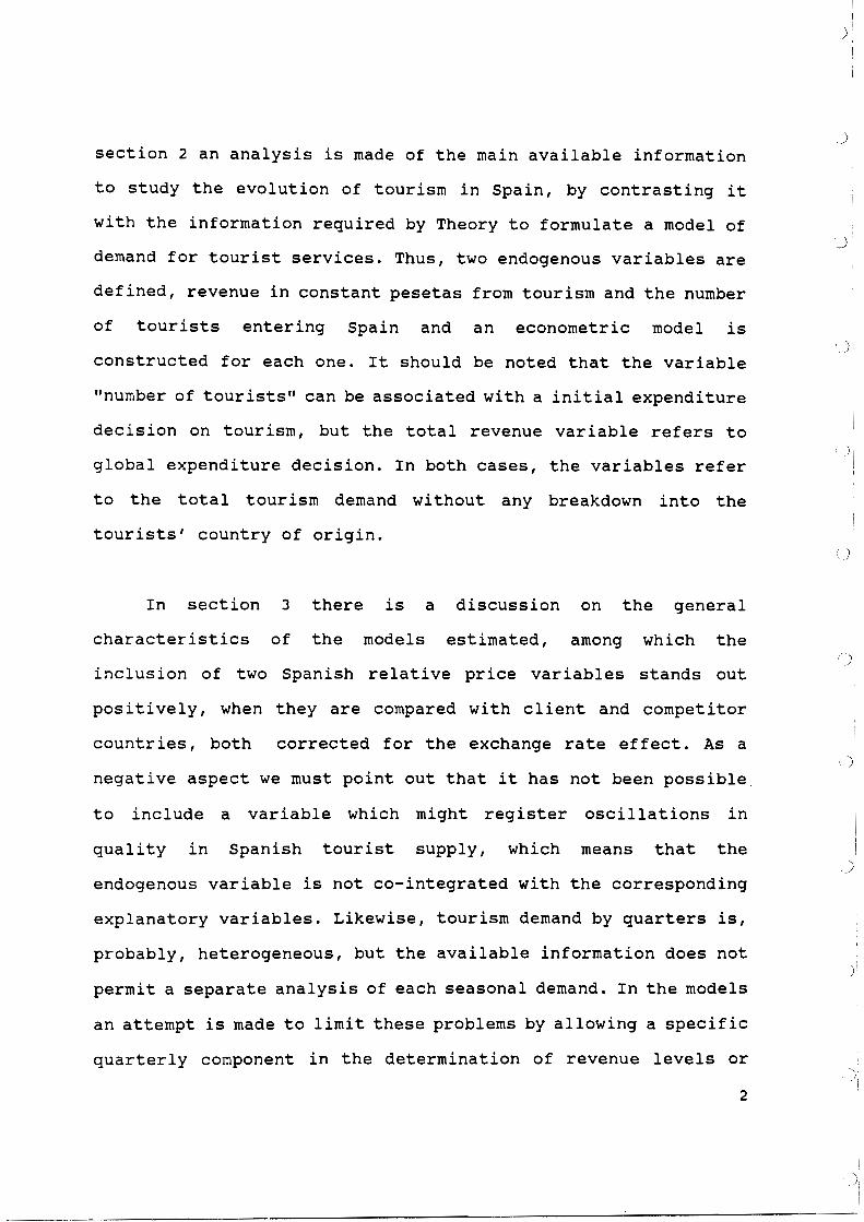
section 2 an analysis is made of the main available information

to study the evolution of tourism in Spain, by contrasting it

with the information required by Theory to formulate a model of

demand for tourist services. Thus, two endogenous variables are

defined, revenue in constant pesetas from tourism and the number

of tourists entering Spain and an econometric model is

constructed for each one. It should be noted that the variable

"number of tourists" can be associated with a initial expenditure

decision on tourism, but the total revenue variable refers to .. 1

global expenditure decision. In both cases, the variables refer

to the total tourism demand without any breakdown into the

tourists' country of origin. . )

In section 3 there is a discussion on the general

characteristics of the models estimated, among which the )

inclusion of two spanish relative price variables stands out

positively, when they are compared with client and competitor

countries, both corrected for the exchange rate effect. As a

negative aspect we must point out that it has not been possible

to include a variable which might register oscillations in

quality in Spanish tourist supply, which means that the

endogenous variable is not co-integrated with the corresponding

explanatory variables. Likewise, tourism demand by quarters is,

probably, heterogeneous, but the available information does not )

permit a separate analysis of each seasonal demand. In the models

an attempt is made to limit these problems by allowing a specific

quarterly component in the determination of revenue levels or

2

tourist numbers. In the case of revenue, this specific component

is deterministic though a certain evolution is allowed for the

component corresponding to winter. In the case of tourists, the

seasonal component is stochastic.

In section 4 there is a description of the econometric

model estimated for real revenue from tourism, and there are

comments on the problems encountered and a development of the

implications which such a model has. From this model several

points stand out: 1) the estimated lag structure for explanatory

variables is compatible with a two-stage spending decision; 2)

the drop in revenue in recent years is explained by a greater

price elasticity, in absolute terms, but it is not possible to

determine which factors have caused such a change in elasticity.

In section 5 a model is estimated for explaining the number

of tourists. The model confirms the possible two-stage aspect of

expenditure on tourism. The seasonal pattern of the endogenous

variable in this case has differentiated traits with regard to

the seasonal behaviour of revenue, which leaves a very important

question hanging in the air: to what extent does the uneven

seasonal evolution between both variables over the years have as

its cause a price policy on the part of the Spanish suppliers

and, if so, in which way is it affecting policy towards the

sector. Unfortunately the available information on prices does

not enable an answer to be given to these questions.

3

The main conclusions of the previous models are recorded in

section 6. There the most remarkable fact is that the income and

price elasticities are different in each stage of expenditure.

Price elasticity compared to competitors is important and acts

prior to elasticity compared to prices from the tourists' country

of origin. Oscillations in demand correspond more to oscillations

in prices than to tourist income.

Section 7 is devoted to recording a group of comments on the

tourism sector which is suggested by the previous econometric

analysis. Thus, the estimated effects of different prices

indicate that the recovery of the sector needs both moderation

in production costs and increased productivity, as well as an

improvement in quality, differentiated supply, etc. In fact, it

does not seem possible that Spain can compete with a massive low­

quality tourist supply. The effect of the appreciation of the

peseta on the evolution of the sector is important. Finally, a

higher number of tourists, does not seem to be possible without

seriously compromising future demand. In any case, this

econometric study of tourism has been seriously hampered by the

lack of available information and, in this sense, the best

recommendation that can be given as a result of it is to

undertake a wide-ranging and regular survey on tourism.

The econometric analysis carried out in this paper hinges

on two indices of relative prices compared to third countries and

corrected for the exchange rate effect. Thus, both prices are

4

)'

, ,

j

) I

i )

. i.

,)

)

-----------------------_._----_._.

merely two indices of the real effective exchange rate for the

tourist sector. This duality of exchange rate indices has been

shown to be of use in explaining the evolution of tourism in

Spain and, also, the estimated models indicate that both indices

have different elasticities and dynamic effects, so that their

aggregation is not recommended. Thus, in section 8, there arise

the implications that these results have when constructing

indices which could be useful in the design and control of

economic policy. The most outstanding of these implications is

that the construction of real effective exchange rate indices

compared to competitor countries is also important, especially

for those sectors of the Spanish economy where competition

largely springs from countries not belonging to the European

Economic Community. The reason is that, in a single market

situation where specialisation in production is favoured, the

sectors with strong outside competition must not rely on a set

of tariff barriers to maintain their competitiveness

artificially, but must pay close attention to the real evolution

shown by this competition and base progress in the sector on

production with differentiated quality in comparison with outside

competition, as well as on an improvement, wherever possible, in

the relative price index. All of the above indicates that, in

order to be able to evaluate the sectoral effects of

macroeconomic policy, the effective exchange rate indices,

consumer prices, etc, which are used in it must not be scalar

ones but vectorial, registering differences which it is

convenient not to ignore.

5

)

)\ 2. AVAILABLE INFORMATION FOR THE ANALYSIS OF FOREIGN

TOURISM IN THE SPANISH ECONOMY

There are basically two types of information: that for

foreign exchange receipts from tourism, which comes from the cash

basis of the Banco de Espana, and that referring to the number . )

• I

!of foreign visitors in Spain. The first type of information is

designed, fundamentally, to serve balance of payments analysis

aims and not to be used for an economic study on the causes )

behind this revenue. Even from the balance of payments viewpoint

the information from the cash basis of the Banco de Espana also

has problems, since revenue from tourism must be accounted for . )

with a downward bias. In fact, this sector is dominated by large

real estate companies with foreign links, which may favour

undeclared tourist revenue inflows being offset by outflows for , )

other reasons.

At the same time, tourist investment in the purchasing of

apartments and property for their own use means that the rents

that tourists must pay to themselves are not registered as

tourist revenue. To register this economic fact would imply

accounting for an outflow of currency for capital revenue (rents)

and an inflow of currency, for the same amount, for tourism. It

should be noted that if the owner of a flat is a foreigner and

he rents it to another foreigner then there should be an outflow

of real estate income and an inflow of the tourist revenue

mentioned.

6

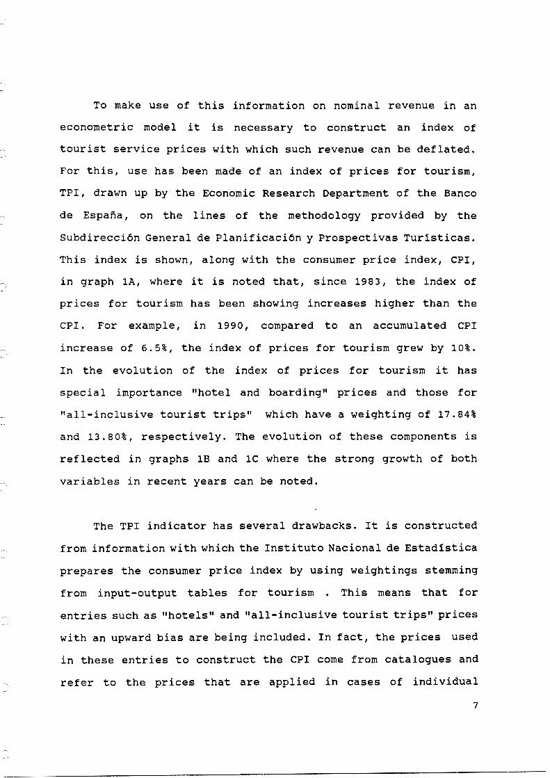
To make use of this information on nominal revenue in an

econometric model it is necessary to construct an index of

tourist service prices with which such revenue can be deflated.

For this, use has been made of an index of prices for tourism,

TPI, drawn up by the Economic Research Department of the Banco

de Espafla, on the lines of the methodology provided by the

Subdirecci6n General de Planificaci6n y prospectivas Turlsticas.

This index is shown, along with the consumer price index, CPI,

in graph lA, where it is noted that, since 1983, the index of

prices for tourism has been showing increases higher than the

CPl. For example, in 1990, compared to an accumulated CPI

increase of 6.5%, the index of prices for tourism grew by 10%.

In the evolution of the index of prices for tourism it has

special importance "hotel and boarding" prices and those for

"all-inclusive tourist tripsll which have a weighting of 17.84%

and 13.80%, respectively. The evolution of these components is

reflected in graphs 1B and 1C where the strong growth of both

variables in recent years can be noted.

The TPI indicator has several drawbacks. It is constructed

from information with which the Instituto Nacional de Estadlstica

prepares the consumer price index by using weightings stemming

from input-output tables for tourism This means that for

entries such as "hotels" and "all-inclusive tourist trips" prices

with an upward bias are being included. In fact, the prices used

in these entries to construct the CPI come from catalogues and

refer to the prices that are applied in cases of individual

7

PRICE INDICES Graph 1 A. Consumer Price Index (CPI)

Tourist Price Index (TPI)

............. 'I J =-1'.. C.P.'... [ [ [, I .. ­180

. . ...••. - ::: T.P.I. ~ 180 .....

.. -_ .... 140

140

120 ~

100 -----r- 120

100

80 I I I I I I I I '80 1.83 1885 ~::~ ;;~;1.84 1888 ---- ---- ----•• a. 1880

COMPONENTS OF TOURIST PRICE INDEX

B. Indices of prices of hotels and lodging C. Index of prices of "alJ.lncluslve

tourists trips" WEIGHTING 17,84'110 WEIGHTING 13,80'110

1nd•• 1.83-100 Ind.x 18.3-100 300 300 240 240

250

100

150

200

V-­/

~

v-~ V­

I~

250

200

100

150

220

120

200

180

180

140

100 -/ - 1/ I'..

v-V V­ 180

180

200

220

140

120

100

50 1883 18.4 1885 1888 1887 1888 1888

--'-------~

1890 50 80

1983 1884 1885 1888 1887 1888 1888 1880 80

~- -~ Iv'J '--- v '-.-­

demand, while a large number of tourists come with "tour

operators", who negotiate much lower prices. Furthermore, the

above-mentioned catalogues are usually revised once a year so

that prices of the entries quoted move in a step manner, without

this reflecting a real fact. With this way of collecting

information, the seasonal pattern of tourist prices is completely

ignored. All of this suggests that for the study of tourism it

would be highly advisable for the Instituto Nacional de

Estadistica to draw up a periodical tourist survey from Which,

among other things, a good price index for tourist services could

be prepared. Despite the above-mentioned drawbacks, and given

that there is no other alternative, in this work the index of

tourist prices described is used.

The study of tourism would require an approach broken down

by countries of origin, since the elasticities of income and

relative prices may be different for tourists originating in

different countries. From the cash basis information series of

receipts from tourism according to countries of origin are

obtained, but their reliability with regard to the country of

origin is very relative, so that the use of this information on

revenue does not enable an analytical study of tourism to be

carried out, and the user is compelled to work with aggregate

models. Finally, it must be mentioned that information on

revenue has a lead and lag problem with regard to the real fact

that it has to reflect, due to expectations of the appreciation

or depreciation of the peseta giving rise to displacements in the

9

) I

)

time of the payments, especially those concerning "tour

operators". Nevertheless, these displacements of payments can be

made only within certain time limits, which enables us to trust, .J

bearing in mind that in this work the information is used in an

aggregated quarterly form, that the above-mentioned problem of

leads and lags will scarcely have any effect upon this study. )

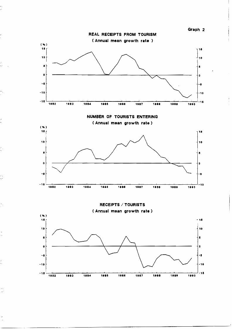
The series of foreign visitors has the advantage of being

a series in real terms and can be directly used as an endogenous

variable of a demand model. The problem arising from the use of

this information is that a study of tourism cannot end with the

econometric explanation of the number of tourists entering Spain,

since real per tourist expenditure is not stable at all, instead

it declines systematically, see graph 2. This means that the

latter must be explained by another econometric model, and, in )

that case, we need to use the information on revenue from the

cash records with the already-mentioned drawbacks. Nevertheless,

approaching the study of tourism through the explanation of two )

variables, the number of tourists entering and expenditure per

tourist, may be very accurate, since in this way one is better

able to register the fact that expenditure on tourism represents )

a decision by stages, firstly - some months before the trip - a

decision is taken as to spending or not, and subsequently, the

amount is decided. If this is true, it may well happen that the

elasticities of income and relative prices will be different in

each decision.

, )

10

( 'll> )

15

REAL RECEIPTS FROM TOURISM

(Annual mean growth rate )

Graph 2

15

10 10

5 5

0 0

-5 -5

-10 -10

-15 1182 1183 1184 1185 118. 1187 1188 1188 1UO

-15

( 'll> )

15

NUMBER OF TOURISTS ENTERING

(Annual mean growth rate)

15

10 10

5 5

0 0

-5 -5

-10 1182 1183 1184 1185 11 •• 1187 118. 1188 1UO

-10

( 'll> )

15

RECEIPTS / TOURISTS

(Annual mean growth rate)

15

10 10

5 5

o 0

-5 -5

1182

-15 L-~

-10

11841183

,-­__......... ~

18.5

"""'~_---I.

18.. '887

-'­'8..

...I....­

18.8

-10

-15 1"0

L...---J

In this paper it has been found that the variable for real

expenditure per tourist is explained much worse than the total

real expenditure (revenue) and it has been decided to limit

ourselves to econometric models on this latter variable. This

result may indicate that measurement errors in revenue and in the

number of visitors accumulate when the expenditure per tourist

variable is constructed. Nevertheless, given that in order to

establ ish diagnoses and recommendations on the sector it is

interesting to know if there are different elasticities in the

possible process of expenditure decision by stages, in the paper

a model is also constructed on the total number of tourists. with

both models real expenditure per tourist can be projected, and

this is a very significant variable, since, for example, a drop

in its value indicates that the same total revenue can only be

achieved with a greater number of tourists, which may mean higher

costs.

Moreover, the use of information on tourists entering allows

an analytical study by countries of origin which is also of

importance for sector planning, if significant differences are

seen in the elasticities of income and relative prices according

to the tourists' country of origin. Given that data on revenue

do not enable an analytical study of demand to be made, in this

paper we will refer basically to aggregate demand, although in

section 5, with the data of tourists according to country of

origin, comments are made on the conclusions of a preliminary

exercise on disaggregated demand.

12

, ) I,

),

)

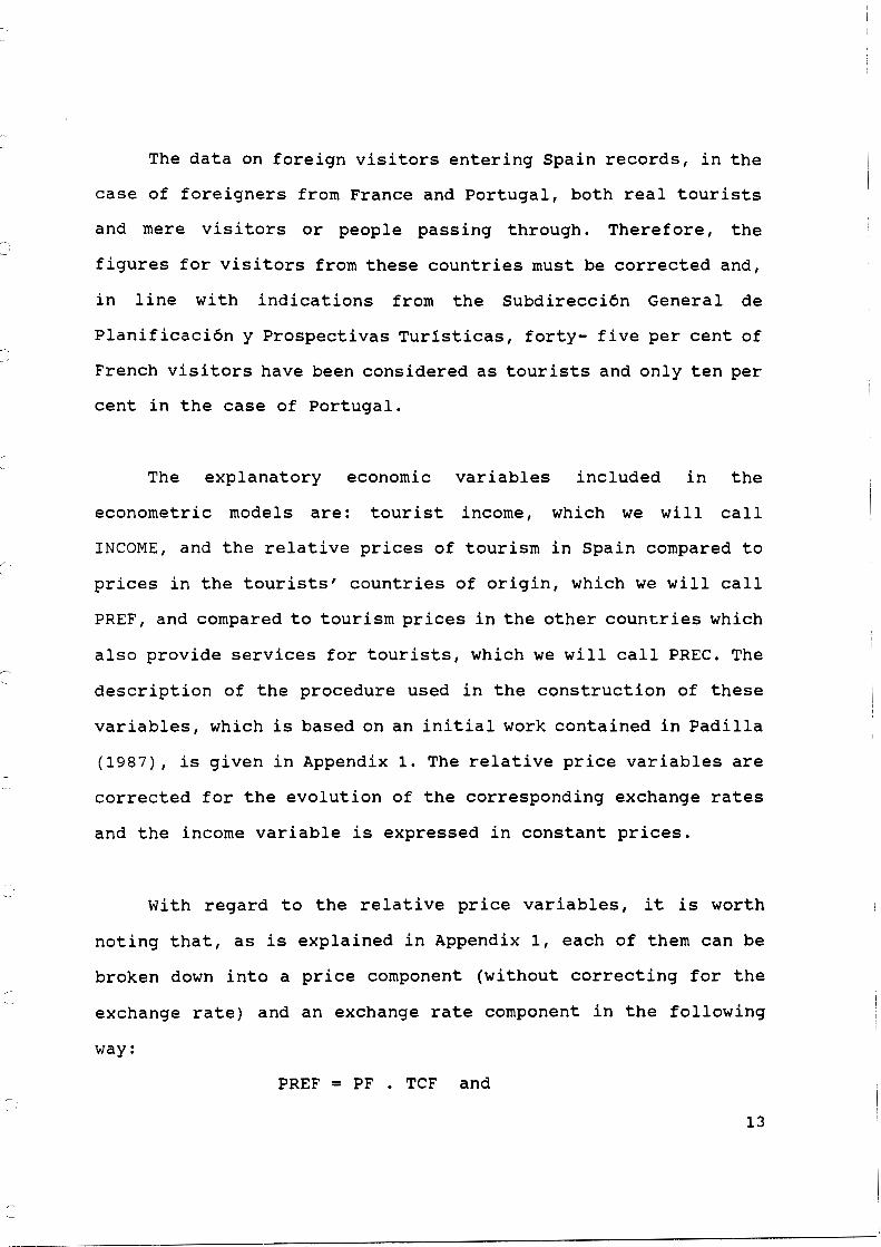
The data on foreign visitors entering Spain records, in the

case of foreigners from France and Portugal, both real tourists

and mere visitors or people passing through. Therefore, the

figures for visitors from these countries must be corrected and,

in line with indications from the SUbdirecci6n General de

Planificaci6n y Prospectivas Turisticas, forty- five per cent of

French visitors have been considered as tourists and only ten per

cent in the case of Portugal.

The explanatory economic variables included in the

econometric models are: tourist income, which we will call

INCOME, and the relative prices of tourism in spain compared to

prices in the tourists' countries of origin, which we will call

PREF, and compared to tourism prices in the other countries which

also provide services for tourists, which we will call PREC. The

description of the procedure used in the construction of these

variables, which is based on an initial work contained in Padilla

(1987), is given in Appendix 1. The relative price variables are

corrected for the evolution of the corresponding exchange rates

and the income variable is expressed in constant prices.

With regard to the relative price variables, it is worth

noting that, as is explained in Appendix 1, each of them can be

broken down into a price component (without correcting for the

exchange rate) and an exchange rate component in the following

way:

PREF = PF . TCF and

13

) I

)

PREC = PC . TCC

where PF and PC are price components and TCF and TCC are exchange )

rate components. Graphs 3 to 6 register these variables.

This breakdown of relative price variables (indices of real

effective exchange rate) is very illustrative since it enables

the contribution of the inflation differential to be separated

from the contribution due to the exchange rate. )

I

The PREF and PREC variables have similar evolutions, compare

graphs 5 and 6, though this is no longer the case at the end of )

the sample. Nevertheless, their corresponding price variables, i

PF and PC, and the exchange rate ones, TCF and TCC, have in each

case, very different behaviour. The latter point stresses a very , >I

important fact with regard to competitor countries. The Spanish

inflation differential compared to these countries has evolved

in a very unfavourable way for them, but the exchange rate )

policies applied have more than compensated for the loss of

competitiveness caused by inflation in those countries.

14

~-,~--~------------------------'------------

Graph 3

RECEIPTS FROM TOURISM IN REAL TERMS

Quarterly .erle. and annual mean

Thouund. of million. of p••• t.. of 1183

1100 r--"i--,..--,----;----r--.,.----,---r---;---;----,.--,...-...,

"00

300

200

1 0 0 L------.........-._._--'-........._"'"--"__.......I.__.............J...........__.....J......__..--.J ............J-.....................J-..................J-......._........J.__........-L............J

1878 1171 1180 1181 1182 1183 188" 18811 1881 1887 1888 1181 1810

Graph 4

REAL INCOME OF COUNTRIES OF ORIGIN

Index 1983. 100

1211 I

120 l-/ ~

1111

V /

/ 110

1011 ~

./l-/

--/ 100

I~\....­III V 10

1178 1171 1180 1181 1182 1183 118" 1185 1181 1187 1188 1181 1110

· )

Graph 5

RELATIVE PRICES COMPARED TO COMPETITOR COUNTRIES

Breakdown by price. and exchange rate.

RELATIVE PRICES COMPARED TO COMPETITORS (PREC)

'40 .------,.--.....,.....---,.--,...--..,.---.....,.....---,..--.---..,.----,----,..--.----. )

'30

120

"0

'00

80 L..-_..:.-_-J..._--l.__l...--_...l--_-J..._-..l.__I.--_...l--_-J..._-..l.__I.----I

'878 '878 '180 '18' '882 '183 '8" '888 '188 '187 '''8 '''8 '''0 )

PRICES (PC .. )

'20 I

"0 .--.1V- I'-----...

"'- ----­'00

80 --~ 80 ~ 70

80 '878 '878 '''0 ,.. , '182 '''3 '''4 '8U '188 '187 '188 '''8

~ '''0 --­

EXCHANGE RATES (TCC·)

2'0 v200 )

'80

/'80 '70 '80

V180

'40 '30 ) 120 /"0 v- ~ '00 to-­../ --­

8,0178 '178 '180 , .. , '''2 '''3 '''4 1888 '''8 '''7 '''8 '''8 '''0

Note: PREC = (PC T x TCC·)/100

The variable PC· and TCC- are the variables PC and TCC explained in the appendix, but on base 1983 = 100

Graph 6

RELATIVE PRICES COMPARED TO COUNTRIES OF ORIGIN

Breakdown by price. and exchange rate.

RELATIVE PRICES COMPARED TO COUNTRIES OF ORIGIN

(PREF)

130

120

110

100

80 1..---..!.:--...J...._.-.J...._--1._......J__.l.--_...J.-_...J...._.-.J...._--1.__I--_J..---J 1878 1878 1880 1881 1882 1883 1884 1885 18.. 1887 1888 1888 1880

PRICES (PF*)

150

140

130 - f-'"120

j../' 110 ~ j........-­100 L.---"

~ 80 J--~

80 V-~70

I 1878 1878 1880 1881 1882 1883 1884 1888 18.. 1887 1888 1888 1880

EXCHANGE RATES (TCF~

150

140 v ~ 130 ~ r-.....120

1\110

100 ~"- ~ -, ./ - - V­

~ 81°878 1878 1880 '88' '812 '813 ,.14 ,... ,.ee '817 ,... ,... '''0

Note: PREF = (PF* x TCF- )/100

The variable PF· and TCF· are the variable PF and TCF explained in the appendix, but on base 1983 = 100

I

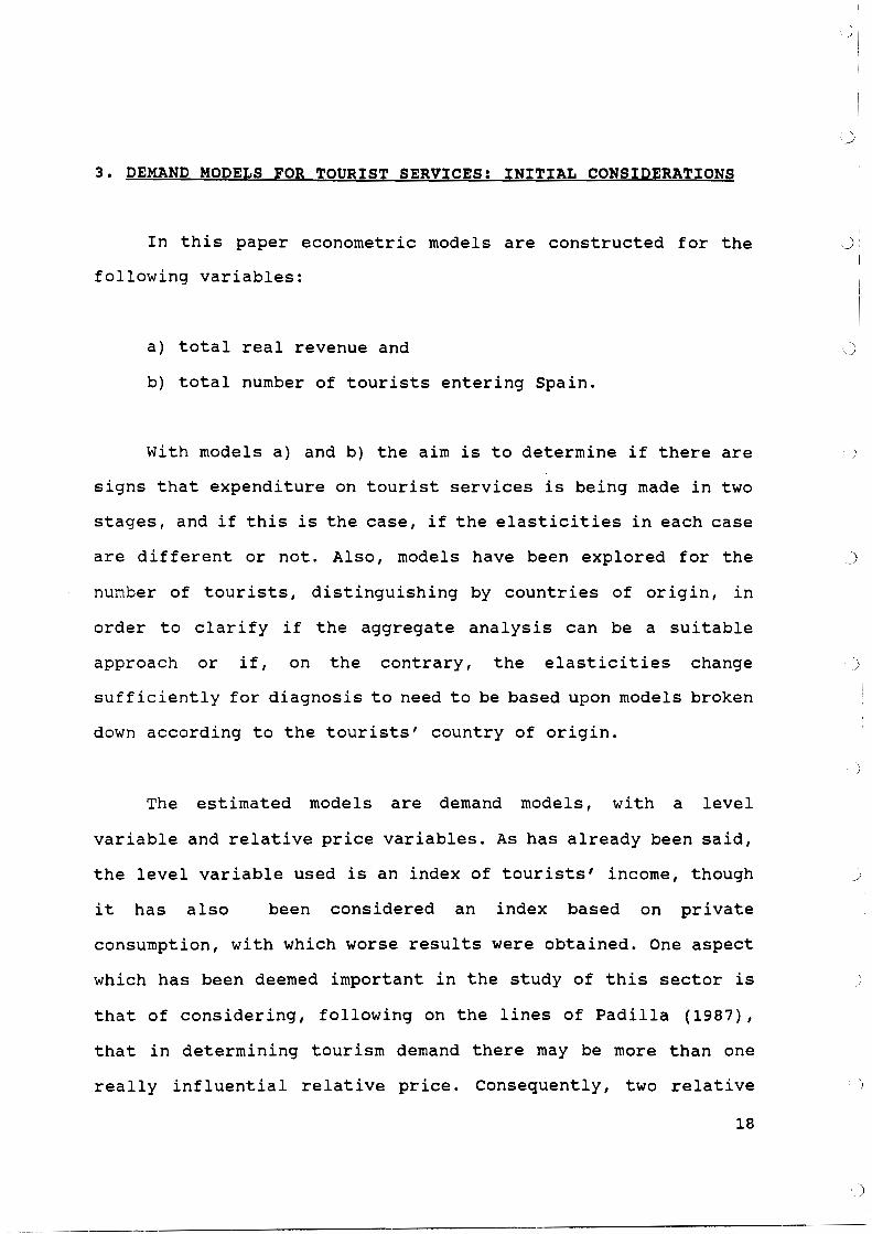
3. DEMAND MODELS FOR TOURIST SERVICES: INITIAL CONSIDERATIONS

In this paper econometric models are constructed for the

following variables:

a) total real revenue and

b) total number of tourists entering Spain.

With models a) and b) the aim is to determine if there are

signs that expenditure on tourist services is being made in two

stages, and if this is the case, if the elasticities in each case

are different or not. Also, models have been explored for the

number of tourists, distinguishing by countries of origin, in

order to clarify if the aggregate analysis can be a suitable

approach or if, on the contrary, the elasticities change

sUfficiently for diagnosis to need to be based upon models broken

down according to the tourists' country of origin.

The estimated models are demand models, with a level

variable and relative price variables. As has already been said,

the level variable used is an index of tourists' income, though

it has also been considered an index based on private

consumption, with which worse results were obtained. One aspect

which has been deemed important in the study of this sector is

that of considering, following on the lines of Padilla (1987),

that in determining tourism demand there may be more than one

really influential relative price. Consequently, two relative

18

._-------------------------------'--'

,)

)

price indices, one for Spain compared to competing countries in

the supply of tourist services and the other for Spain compared

to the tourists' countries of origin have been used. The evidence

in favour of the fact that both indices influence the

determination of tourism demand in Spain, will imply that the

improvement in Spain's competitiveness compared to the countries

of the European Community is not enough to maintain sustained

growth in tourist revenue, if it is not also accompanied by an

improvement in competitiveness compared to countries

traditionally providing tourist services and compared to new

countries which might add to the supply of world tourist

facilities. We will return to this point in the next section.

As is explained in Appendix 1, the relative price variables,

which have had to be constructed from consumer price indices in

the different countries, are corrected for variations in exchange

rates and are formulated as chained indices the weightings of

which change over time. Nevertheless, these indices do not take

into account the relative changes in quality in Spanish tourist

supply, from the one referring to the transport and

communications infrastructure, overcrowding in tourist centres,

care of the beaches, etc, to personal attention in hotels. Nor

has an indicator been found which might make an acceptable

approach to the evolution of this variable which we could call

"qua 1 i ty of spanish tourist supply". Therefore , it has been

assumed that this quality variable follows the type of

stochastic process called random walk, that is, quality in moment

19

I

t equals that of the previous moment, t-1, plus a change which

is unpredictable. This implies that tourism demand is not co­

integrated with tourists' income and the relative price indices

used, but that the possible co-integration relationship should

include a variable on tourist quality which is unknown. Given all

that, the model cannot be formulated to determine the level of

demand but has to be formulated on differenced variables.

As will be seen later on, there are signs that the quality

of spanish tourist supply could have been increasing during a

large part of the eighties, but it could have stagnated in the

final years of the decade. By accepting this type of information,

dummy variables of the ramp-type could be constructed, as was

done in Espasa et al. (1990). When this is done, worse

adjustments are obtained than those given here or the only

significant variables are the dummy ones. Therefore, in this

paper, as has been indicated, changes in quality are assumed to

be stochastic and the model is formulated with variables in

differences. 1

Tourism demand has a very marked seasonal oscillation.

Nevertheless, none of the explanatory economic variables contain

In Espasa et al.(1990) and Espasa and Scheepens (1992), adjustments with ramp-type variables were good and maintained the significant effect of the explanatory economic variables. That was due to errors in the construction of the income and relative price variable compared to competing countries, which have been eliminated from this work.

)

) !

~ ) ,

)

, 1 j

)

20

seasonal movements2 , so the seasonal pattern of the dependent

variable must be deterministically explained, by means of

seasonal dummy variables, or, stochastically, by means of a

residual component generated by an autoregressive process with

unit roots of seasonal periodicity. The latter, along with the

need to differentiate the variables due to the effect of changes

in quality, implies that modelmaking of tourism demand with a

stochastic seasonal behaviour requires formulating the variables

in seasonal differences.

~ Specifically, the relative price indices do not have a seasonal pattern, since they have been constructed from the consumer price indices of the corresponding countries which hardly show seasonal changes and the income index, for reasons of homogeneity in the availability of data, has been constructed from seasonally adjusted series of real income of different countries.

21

--------~---------------_._---

4. AN ECONOMETRIC MODEL FOR DETERMINING REAL REVENUE FROM FOREIGN

TOURISM

The dependent variable - which we shall call IRT -is defined

as nominal revenue deflated by the index of tourist prices

commented on in section 2. The explanatory economic variables are

the ones pointed out in that section, INCOME, PREF and PREC.

In model 1 in table 1 the dependent variable IRT is

explained on the basis of the above-mentioned variables and a set

of dummy variables. The elasticities have the expected signs,

both relative price indices enter, the one corresponding to

competitor countries with a four quarterly lag and that for

tourists' countries of origin in contemporaneous form, that is

with no lags.

In the construction of this model we began by testing

whether the endogenous variable and the explanatory ones were co­

integrated or not. When the co-integration relationship was

rejected, this being justified by the absence in the model of a

variable which could record movements in the quality of tourist

supply, we went on to construct the model by using the variables

in first differences. Initially, a model was formulated with the

most dynamic specification that the data allowed and,

sUbsequently, it was simplified until we concluded with the

indicated one.

22�

)

,) ..

)

)

)

)

( ") (" \, (' ,� ( f \ "\ \

Table 1

ECONOMETRIC MODELS ON EXTERNAL DEMAND FOR TOURIST SERVICES IN SPAIN

Model Dependent Number Variable EXPLANATORY VARIABLES RESIDUAL ELEMENT

AND INCOME PREC PREF Seasonal Impulse Other ADJUSTMENT

dummy dummy variables (In) (In) (In) variables variables

I

1 (l-L)lnIRT 1. 56 L3 -0.81 L4 -0.90 Appear with -0.l1D812 O.lWINTER White noise. Standard (2.53) (3.59 ) (4.10) restriction (4.11) (6.12) deviation of the in­

of� sum zero novations 0.034. The -0.08D841 Box-Ljung test does

(2.91)� not reject the hypothesis of white noise for the innovations. These are shown in graph 7.a. R2=0.99

2 (l-L)lnIRT 1. 75 L3 -0.77 L4 -0.69PREF Appear with -0. 11D812 O.lWINTER White noise. Standard (3.05) (3.69 ) (3.18) restriction (4.43) (7.07 ) deviation of the in­

of sum zero novations 0.0324. The -1. 69PREF89 -0.08D841 Box-Ljung test does (2.78)� (3.18 ) not reject the hypothesis

of white noise for the innovations. These are shown in graph 7.b. R2=0.99

Table 1 (Cont.)

ECONOMETRIC MODELS ON EXTERNAL DEMAND FOR TOURIST SERVICES IN SPAIN

Model Dependent Number Variable EXPLANATORY VARIABLES RESIDUAL ELEMENT

AND INCOME PREC PREF Seasonal Impulse other ADJUSTMENT

dummy dummy variables (In) (In) (In) variables variables

3 (1-L4) lnTUR 2.3 L2 -0. 5 6L4pREC 0.06EASTER AR(l) process with (4.3) (2.91) (3.3) coefficient 0.3 (2.1).

-1.06L4pRECBB Standard deviation of the innovations 0.055. The

(2.41) Box-Ljung test does not reject the hypothesis of white noise for the innovations. These are shown in graph 9.a. RZ=0.99

4 (1-L4) InTUR 2.4 L 2 -0. 56L4pREF 0.06EASTER AR(l) process with (4.6) (3.0) (3.6) coefficient 0.3 (2.1).

-1. 32L4pREFBB Standard deviation of the

innovations 0.054. The (2. B) Box-Ljung test does

not reject the hipothesis of white noise for the innovations. These are shown in graph 9.b. RZ=0.99

NOTES:

- All the explanatory variables, except the seasonal dummy variables, enter each model with the same differentiation applied to the corresponding endogenous variable.

- L is the lag operator and is such that VX. = X'.j In the columns corresponding to the explanatory variables the operator V appears, when the variable in question enters the model j periods lagged. When nothing is indicated, the effect is contemporaneous. Under the coefficients the statistics t appear. The impulse variables are defined as OAT, where A indicates the year, with two digits, and T the quarter, in which the corresponding variable takes the value unit. At all other moments, the values for an impulse variable are zero. The variables that appear in the "Other variables" column are dummy and are explained in the text.

o\---j ~"

'-.-'

In this model the INCOME variable has a three-term lag.

This lag effect, along with that for relative prices with

competing countries, is compatible with a two-stage spending

decision: in the first, some quarters before the trip, on the

basis of income and relative prices in spain compared to those

of competitors, it is decided whether to come to Spain or not,

and, subsequently, at a present time, mainly on the basis of

relative prices in Spain compared to those of the countries of

origin, the extent of the expenditure is decided.

The evolution of the two relative price indices, or indices

of the real effective exchange rate, has been quite similar

throughout the sample, except in the last two years. Thus, the

incorporation of both indices in the model is based fundamentally

on a different dynamic structure. In any case, the response

distributed in the time of the dependent variable with regard to

the real effective exchange rate enables an explanation to be

given for tourism demand as expenditure carried out in two

stages. Which is the most important real effective exchange rate

index at each stage, is rather more debatable, given the

similarity of both indices in the sample used. At the same time,

this similarity emphasises that both exchange rate indices are

important, so that none of them is to be ignored. Compared to the

alternative of grouping both indices in just one real effective

exchange rate index, which could consider both client and

competitor countries, in this paper it was decided to use both

separately. With this breakdown of competitiveness into an

25

I I

) I

indicator with regard to countries with tourism demand and those

with supply, it is possible, subsequently, as is done in graphs

5 and 6, to make, in each case, a separation of the effect due

to the inflation differential from the effect corresponding to

the nominal effective exchange rate. These effects have been

radically different in one index and another and it would appear

convenient to continue carrying out a detailed pursuit of the

differential effects of inflation and the exchange rate with the

two groups of countries.

This pursuit of the four components of the sector's

competitiveness, two for each group of countries, has an interest

that goes beyond the formulation of econometric models. The

decline of competitiveness compared to the other countries

offering tourist facilities, despite the favourable advantage for

spain with regard to the inflation differential with them, which

has been observed since 1984, could have greater subsequent

effects, if the peseta appreciates in comparison with client

countries' currency, without a reduction of the differential of

inflation compared to the latter being achieved. Such an

appreciation has been produced from 1988-89 and, as will be

discussed below and also in the following section, from these

years onwards elasticity of demand compared to relative prices

may be considered to have increased. That is to say, the demand

registered by the sector may be sUbject to non-linear structures

that might be less diff icult to detect and comprehend on the

basis of the four components defining the competitiveness of the

26

. )

)1i

\ , )

')

J� I I

sector.

In graph 7a the residuals of model 1 are recorded. There a

concentration of negative residuals, high in absolute value, can

be seen in 1989 and 1990; likewise, there is a concentration of

positive residuals from 1984 to 1986, except for 1985. The

interruption of the sequence of positive residuals during 1985

could be due to the fact that in the summer of that year the

international press gave fairly wide coverage to the terrorist

attacks which took place in Spanish tourist areas.

A model capable of registering the drop in tourism in 1989

and 1990 is difficult to obtain. One possible solution is that

elasticity of relative prices in Spain compared to tourist­

supplying countries is not constant, so that, when loss of

competitiveness goes beyond certain levels, it has greater

effects. Apart from what has been previously indicated on the

four components defining competitiveness in graph 6, it is noted

that between 1988-89 the PREF variable began to show values above

the historical maxima registered at the beginning of the sample.

Furthermore, by analysing the exchange rate indices - graphs 5

and 6- it can be seen that it is also from 1988-89 onwards that

the peseta began to appreciate both compared to competing

countries and those of the tourists' countries of origin, with

a huge appreciation compared to the former. To the extent that

exchange rate information is more accessible and more widely

pUblished, it could occur that this type of appreciation

27

Graph 7a

RESIDUALS OF MODEL 1

0.08 r-...,....--..,---r---r---.,.--...,..--...,....---,---,...----,-----,.--...,..------. 0.08

0.07 _.----­ _.----­ -.----­ -------­ ------­ ------­ ------­ -------­ ------­ ------­ -.--.-­ -.----­ 0.07

0.01 0.01

0.05 0.05

::: f\..! ~ I :::: ::: A· \ I \I[\ ~ I \ :::

-0.0:

-0.02 -0.03

-0.04

-0.05

-0.01

-0.07

-0.08

~ (\ ~ \ ,I \,... 7

~"/ _. ._ _ .___

V -----.­ -------1------­ -------­ ------­ ------­ ---_ .. ­ ----.--­ ------­ -.----­ ----­ - ------­

L..-~_~-'-...................l.._,,~~ ........._---'_.............l.~............J...........~...J-....................._ ................_ ........_........;i:...J.._..............J....---J

1171 1.. 0 1.. 1 1..2 1.. 3 1..4 1"11 1"1 1"7 1... 11'1 1..0

~o.o 1

-0.02 -0.03

-0.04

-0.05

-0.01

-0.07

-0.08

)

Graph 7b

RESIDUALS OF MODEL 2

0.08 .-----..,.....--.,......--,....---.,.---,..--..,...---,---..,..---,...---.,.----.---......---.

0.07 r­

0.08

0.08

0.07

0.01

0.02

0.01

-o.o~ -0.02

::_:: -0.01

-0.07

-0.08 1171

•

T \

, I .~.....

11.0 1.. 1

IV

1..2

~

1\ \1 ~

1"3

~

I1 ~ V .____

1..4 ,... 1..1 1"7

"\ I1 \

/-... ...1.....

11.. 11.. 1.. 0

0.02

0.01

~0.01 -0.02

:::: -0.01

-0.07

-0.0'

,i)

determines a period when tourists are more sensitive to relative

prices, with an increase, in absolute terms, of expenditure

elasticity related to these prices. Also, to the extent that

tourist summer overcrowding in Spain was historically the highest

in 1988 - see graph 8 -, and to the extent that overcrowding

means a loss of quality of service, it holds that greater

elasticity with regard to prices in the most recent years of the

sample can be justified by a loss in quality.

There are, consequently, various reasons for thinking that

elasticity with regard to prices may be greater in recent years.

This may be built into the model, by introducing the PREFX

variable, which takes zero values till the last quarter of the

year (X-I) and the value of PREF from the first quarter of year

X. This is done in model 2 in table 1, where it is observed

that, from an elasticity of -0.69 up to 1988, it moves to another

of -2.38 from 1989 onwards. Thus the adjustment is improved and

a more acceptable residual behaviour is obtained in the last

years (see graph 7b)3.

We tried putting the extra effect from 1989 onwards on the

PREC variable but the best result was the one obtained in model

2: in fact the extra effect is not significant with the PREC

variable. Model 2 indicates that the drop in tourism in recent

years can be explained by a greater elasticity with regard to

3� The PREFX variable has been introduced into the model so that, once it has been differentiated, it affects the dependent variable from the first quarter of 1989 onwards.

29

J.�

prices, although there may be several reasons for that changing

elasticity. Unfortunately, the sample is excessively limited for

discriminating as to which factors and to what extent determine

that change in elasticity.

If we add to model 2 a ramp-type dummy variable beginning

in 1980 or 1984 and ending in 1986, or a doubly ramp to take into

account the large drop in 1985, the adjustment is improved, all

the economic variables maintaining their significance, though

there are certain changes in the coefficients. Thus, income

elasticity may fall to 1.3 and that of PREF be of -0.25 until

1987, with the elasticities and coefficients of the dummy

variables remaining almost the same. This indicates that if the

model is omitting one or several important variables, such as,

perhaps, improvement in commercialisation and quality in Spanish

tourist supply in those years, which might allow an approach

through the above-mentioned dummy variables, that omission may

be giving an upward bias to income elasticity.

Nevertheless, these ramp-type effects may be considered

slightly arbitrary, so the models including them were rejected,

and model 2 from table 1 was chosen as the pattern to use in

formulating an approach to the behaviour of real revenue from

tourism.

All the previous models assume that tourism demand is

homogeneous in the different quarters of the year. This is hardly

30

: \

)

)

I

---------------------------

likely to be the case and, more probably, the tourist sector has

to deal with at least two different demands; summer and the rest

of the year. Thus, for example, as can be seen in graph 3,

revenue in the first quarters has fallen less in recent years

than revenue from the third quarters. This fact is not explained

by movements in income and relative prices, so it may be a

question of different demands, that is, with different

elasticities4 • Unfortunately, the number of observations

avai lable does not enable a reliable estimate of models with

di fferent elasticities of income and pr ices according to the

quarters of the year. To alleviate this imperfection, a WINTER

variable has been built into the model which takes value one in

the first quarters of 1988 and successive years and zeros at

other times. This variable appears as very significant and thus

records the fact that winter tourism has different

characteristics and, specifically, has shown less of a drop in

the last few years.

The model includes two impulse dummy variables to correct

outliers: those corresponding to the second quarter of 1981 and

the first quarter of 1984.

The specification of the model also contains highly�

significant seasonal dummy variables. The seasonal pattern in the�

variable (l-L)ln IRT which is derived from them is:�

4� Relative prices have been constructed by using the consumer price index of the corresponding countries� and these indices do not register possible seasonal changes in tourist prices.�

31

First quarter: -0.22�

Second quarter: 0.27�

Third quarter: 0.43�

Fourth quarter: -0.48.�

Nevertheless, seasonality is a cyclical oscillation which

has its main interest when calculated on the level of an economic

phenomenon. Therefore, it is important to calculate the

corresponding seasonal coefficients for tourist revenue in real

terms, which is derived from the seasonal coefficients estimated

in the econometric model on (l-L)lnIRT. Pierce (1978) calculates

the relationship between the seasonal coefficientsS of a variable

on levels and first differences. For quarterly series this

relationship is:

j 1 4 Bj = I: 0; + I: h j = 1, ... ,4

i=l 4 h=l

where (3 and 0 are seasonal coefficients corresponding to the

level and first differences, respectively. By applying such a

relationship to revenue from tourism we find that in the third

quarter there was a seasonal increase of 40.25%, while in the

first, second and fourth quarters there were cyclical falls of

29.75, 2.75 and 7.75%, respectively.

5� An application to Spanish data is found in Espasa (1989), pages 408 and 409, where on an ARIMA model for the monthly industrial production index, January 1965 - December 1982, the magnitude of the seasonal change is calculated from January 1975 onwards, a time when there was a confluence on the data of this brought about by change in the survey used for calculating it and the effects of the energy crisis.

32

)

)j

)

I

.. ). i

)

)

These quarterly seasonal coefficients do not, in any way,

reflect, except in the first quarters, a homogeneous seasonal

behaviour in the months of each quarter. In fact, in Espasa and

Scheepens (1992) a monthly seasonal IRT profile is calculated and

it is observed that the seasonal factors increased from April to

August and fell from September to December, rising once more,

almost to the April level, in the first three months of the year.

Over the years the seasonal factors of each month in real tourist

revenue has remained fairly constant, with a simple noteworthy

feature being a certain growth of the seasonal coefficient for

the month of May.

33

)

s. AN ECONOMETRIC

ENTERING SPAIN

MODEL FOR DETERMINING THE NUMBER OF TOURISTS

i

Ji I ,

In graph 8 the quarterly series of tourists entering Spain

from abroad, TUR, is shown. In the graph it can be seen that it

is a series which is dominated by the seasonal component. One can

also detect that, after ten years of continued growth in the

figures for tourists arriving in Spain -except for 1982 which,

from the present day point of view, can be considered episodic -

in 1989 that figure is stuck at 1988 levels and in 1990 began

to decline.

)

'.)

When estimating demand models such as those of the previous

section to explain the number of tourists, the following facts

are of the greatest significance:

1. The economic variables, number of tourists, tourists'

income index, relative price index, compared to client

countr ies and the relative pr ice index compared to

competitor countries, are not co-integrated either and

the model must be formulated on differences.

.J

2. The seasonal pattern of the dependent variable, as in the

previous section, cannot be explained by means of the

economic variables considered, but, unlike what occurred

wi th revenue, now this seasonal behaviour is better

recorded by means of a stochastic structure.

34

. )

~( ( )\ ,

Graph 8

( )(, !

TOURISTS

Thouaanda 0' people

18000 15000

14000 r- - 14000

13000 - - 13000

12000 ­ 12000

11000 f- - 11000

10000 f- - 10000

r- - 9000

8000 - - 8000

7000 ­

9000

- 7000

8000 - - 8000

- 50005000 ­ I ~ N I~

- - 40004000 \J ~ I\JU \j N 30003000 f­ ~ N ­

20002000� 1878 1878 1950 1881 1982 1883 1984 1985 1888 1987 1988 1989 1990�

)

Consequently,

differences.

the model is formulated on annual

3. Only one price effect is recorded, PREF or PREC, but

never both together. In any case, the data require

prices to appear in the model with a time lag of four

quarters.

4. Whatever price variable may be used, its corresponding

elasticity is not constant but increases, in absolute

value, at the end of the sample.

... )

5. The global adjustment is practically the same, regardless

of the price variable used. Likewise the elasticities

obtained are almost identical in both cases, the biggest

difference being in the elasticity compared to prices in

the final part of the sample, which with PREF is -1.3

and with PREC -1.1. The differences in adjustments are

given in the last three years, and the adjustment with

PREF is marginally higher.

I

),

. )

6. The number of tourists entering Spain each quarter is

sensitive to the fact that the Easter holiday falls in

the first or second quarter. Thus, it is necessary to

include a dummy variable to evaluate the influence of

the Easter holidays in the rise noted in tourist numbers

in those quarters when these holidays occur. For this

36

)

purpose, it has been considered that the "Easter effect"

covers the period running from the Friday prior to Holy

Week to Easter Sunday, both inclusive; in this way a

dummy variable is constructed, called EASTER, which

always takes value zero in the third and fourth quarters

every year and a value between zero and one in the first

and/or second quarters, depending upon the proportion of

days of the period mentioned belonging to those quarters

each year, so that the sum of the values this variable

takes in the first two quarters is equal to the unit.

7.� The residual element follows a first order autoregressive

process.

8.� Unlike the econometric models on expenditure in the

previous section, where the seasonal pattern was

modelled in a deterministic, stable manner, in the

models on the number of tourists seasonality is of a

stochastic type. As a result, its level evolves over the

years, though in the absence of future disturbances,the

seasonal coefficients would each tend towards a stable

level. The stability of the seasonal pattern of

expenditure and a relative seasonal evolution in the

number of foreign visitors appeared initially in Espasa

and Scheepens (1992), where both seasonal profiles are

illustrated and quantified. In that paper it is shown

that the seasonal peaks for the months of July and

37

J�

August in the number of tourists have been reduced in

the eighties, moving from coefficients slightly above I

150% in 1982 to values around 125% in 1989. This slight I i

Y Iflattening out of the summer peak for tourism6 is

something which in principle must be considered as

positive for permanent supply, that is, areas which do ,� ) ~

not close outside the summer, of tourist services.

Nevertheless, this reduction in the seasonal cycle of

visitors is not reflected in real revenue, which apart

from leads and lags problems, indicates that the

seasonal peak of real expenditure per tourist may be

rising in the months of July and August? To what extent

this effect is due to a greater increase in relative

tourist prices in the summer than in the other months of

the year, or to an income effect is, undoubtedly, an )

interesting subject for subsequent studies.

In table 1 two models are shown for explaining the number

of tourists entering Spain each quarter, one using relative

prices compared to competitors and the other compared to

tourists' countries of origin. As has been indicated before, the

data are not able to discriminate between the importance of one

6 It should be noted that the seasonal cycle is measured as a percentage of an annual level, so the reduction� summer peak does not necessarily indicate that the number of summer tourists has been falling in those� years. In fact, graph 8 indicates that this number has grown throughout the sample.�

7� Once more, the increase in this seasonal peak is in relative terms on average annual expenditure, so that� if the laller is falling, the seasonal rise may not imply an increase in real expenditure per person in the� summer months over the years.�

38

price index or another for this dependent variable. Therefore,

given that the only price variable in these models always enters

lagged four quarters, and given that in the model on revenue in

the previous section the prices showing this lag were the

competitors', it is proposed to use the model with relative

prices compared to competitors -model 3 in table 1-. The

residuals of both models 3 and 4 are recorded in graphs 9a y 9b,

respectively.

The model obtained for the number of tourists also favours

the explanation that expenditure on tourism takes place in two

stages, since all the economic variables which enter into the

determination of the number of tourists - a variable which can

be considered to correspond to the first stage in the expenditure

process- appear with lags.

With the information on the number of tourists an analysis

can be made of tourism demand broken down on the basis of

countries of origin. In this paper a certain exploratory analysis

has been made and from it it is deduced that elasticities and

even the lags with which the explanatory variables appear are

different according to the countries of origin. This suggests

that a recommendation for future works is to carry out an

analytical study according to countries of origin.

39

)

Graph 9a

RESIDUALS OF MODEL 3

0.12

0.1

0.08

0.01

0.04

0.02

o

-0.02

-0.04

-0.01

-0.08

-0.1

-0.12

-----­ ------­ -_.. ­ - -----­ ------­ -----­ ------­ -----­ ------­ ------­ -----­ ------­ -----­

-1

~ l /\ I1\ rJ I~ V

V ~ V/ I

V -----­ ------­ .. -­ ---­ -----­ ------­ -----­ ----- .. ­ -----­ ------­ ----_ .. - -----­ -... _---­ -----­

I

1178 1.7. 1880 1881 1882 1883 1884 1.88 1881 1887 1888 1181 1110

0.12

0.1

0.08

0.01

0.04

0.02

0

-0.02

-0.04

-0.01

-0.08

-0.1

-0.12

' )

Graph 9b

RESIDUALS OF MODEL 4

0.12

0.1

O.OB

0.06

0.04

0.02

o

-0.02

-0.04

-0.06

-O.OB

. !

------l-------~----- - -----­ ------­ -----­ ------­

NII /\ " I V

V ....

-----­ ------­ ------­ -----­ ------­

\

!'r\ I\..

V \ I

~ V

-----­

V -0.1 -----­ ------­ ------­ -----­ ------­ -----­ ------­ -----­ ------­ ------­ -----­ ------­ -----­

-0.12 117B 117. 1880 1881 1882 1183 1.... 1188 1181 1187 1188 1181 1110

)

) \

I

6.� MAIN CONCLUSIONS OF THE ECONOMETRIC MODELLING

1.� An econometric analysis of external demand for tourist

services in Spain can be made through a series of

receipts in foreign currency under this heading or

through the series of tourists entering. Both present

problems. To base a study on the first ser ies means

constructing a price index with which to deflate

revenue, but the systematic information on what tourists

pay via "tour operators" is not available, so the index

of tourist prices used in this work may have upward

biases. If the study is made only on the number of

tourists, it is found to be incomplete, since

expenditure per tourist is not at all constant (see

graph 2). From the above, it can be seen that, in order

to have a full knowledge of the tourist sector, model­

making of both variables is convenient. What is more,

the formulation of models both for the number of

tourists and for expenditure make~ it necessary to be

able to explain the demand for tourist services as

expenditure decided in two stages.

2.� In the demand models estimated, it is found that the

corresponding endogenous variable is not co-integrated

with explanatory ones: an income variable and two

relative prices in Spain compared to competitor

countries and compared to tourists' countries of origin.

41

That is, its long term evolution is not solely

determined by the above-mentioned economic variables.

Probably there are omitted variables and among them the

outstanding ones are the increase in supply and

oscillations in its quality. In this paper the absence

of co-integration among the variables is dealt with by

formulating the model in logarithmic differences.

3.� The results obtained are compatible with the explanation

that expenditure on tourist services takes place in two

stages. In the first, some months before the trip, on

the basis of the tourists' income and relative prices in

Spain compared to competitors, it is decided whether to

come to spain or not, and, in the second, on the basis

of income and relative prices in Spain compared to

countries of origin, the magnitude of the expenditure is

decided. Income elasticity in the first stage -2.3

(±a.5)-seems higher to that of the second. The global

elasticity which is estimated for the two stages is 1.75

(±a.6) .

These elasticities could be upwardly biased if in

the models the probable quality increases in Spanish

tourist supply in the first two thirds of the eighties

are not considered. A possibly more accurate value for

42

)

),

)

. )

)

the last mentioned elasticity may be 1.3 (±O.6)8. As far

as elasticity regarding prices is concerned, what is

obtained is better, in absolute terms, in the second

stage than in the first.

4.� Tourist income is highly dominated by a trend evolution,�

so oscillations in tourist service demand are basically�

linked to relative prices.�

5.� The drop in tourism in recent years can be explained with�

models of changing elasticity regarding prices, so that�

this has increased, in absolute terms, in recent years.�

Nevertheless, the causes of this greater elasticity are�

not easy to identify. Thus, the following can be pointed�

out:�

a) it is a non-linear type economic relationship;

b) given that information on exchange rates is more

widely and quickly made available, the huge appreciation

of the peseta compared to competitor countries along

with an appreciation compared to the tourists' countries

of . origin, which took place in recent years, has

increased price sensibility.

c) the quality of the Spanish tourist supply has not

increased at the previous rate or has even fallen in

8 This is the value which is obtained in models which include ramp-type dummy variables in the middle of the sample.

43

._--­

)

recent years, and, in the absence of a suitable

explanatory variable, this model records it as a greater

elasticity towards prices. If greater tourist

overcrowding is an indicator of lower quality of tourist

services, we would have that this quality must have

fallen from 1988 onwards, a time when the highest number

of foreign tourists was recorded.

In any case, all these explanations coincide in

assigning the recent fall in demand for Spanish tourist

services to the negative evolution of relative prices.

6.� Demand shows a very strong seasonal behaviour, while the

explanatory economic variables do not contain seasonal

oscillations. The seasonal pattern of demand possibly

means different elasticities of income and prices in the

summer compared to the rest of the year. Nevertheless,

there is not enough information to estimate all those

elasticities and the model approaches them by means of

dummy variables and/or seasonal autoregressive

processes.

Specifically, the result is obtained that winter

tourism (first quarters) has been less negatively

affected in recent years than tourism in the other

quarters.

44�

J

, )

.>

. )

)

)

I I

)

I )

I

7.� The exploratory study, which has been made of demand

models broken down into countries of origin, indicates

that dynamic effects and income and price elasticities

may be quite different according to the tourist's

country of origin. This indicates that a future research

analysing tourism in Spain, disaggregated by countries,

would be interesting.

45

I

._-------------------------_._-_._-------------'

7. SUGGESTIONS APPLYING TO THE SPANISH TOURIST SECTOR WHICH CAN

BE DERIVED FROM THE ECONOMETRIC ANALYSIS CARRIED OUT

Of the variables determining tourism demand there is one,

tourist income, which cannot be influenced by Spanish economic

agents and their action, consequently, is limited to relative

prices Which, furthermore, are the ones that have caused the

recent drop in tourism in Spain. In this sense, it is worth

making a series of clarifications and suggestions.

spanish tourism demand depends on two relative prices, so

improving only one, with regard to competitor countries, does not

completely solve the problem.

The price indices used are, obviously, corrected for

variations in the exchange rate and can be broken down into a

pure price component and another of corrections due to exchange

rate. On seeing this breakdown in the index compared to

competitor countries a highly favourable recent evolution

(negative) for Spain is observed in the price component - graph

5 -. Nevertheless, this evolution does not so much indicate a

policy of price restraint and productivity increases in the

Spanish tourist sector, but rather continuing periods of high

inflation in several competitor countries. Therefore, on seeing

the evolution of the peseta exchange rate index compared to those

countries it is noted that they have resorted to devaluation, not

just to maintain competitiveness but to increase it. That is, in

46

, '\

)

, .1!

! )

)

)

,)

c several of these countries what has happened is that high

inflation has brought about loss of competitiveness, and a bid

c to recover or even increase it has been made by devaluation,

which, sooner or later, has been translated into price increases

that lead to this spiral ~eaction being perpetuated.

c It is not easy to determine how long these countries can

continue with those policies, but perhaps long enough to cause

c serious damage to the sector in Spain. What is more, competition

for tourism is being joined increasingly by countries with a low

degree of development, who are going to be ready to enter the

c inflation-devaluation spiral. If the above is true, the Spanish

tourist sector can do very little in this respect, since all

increases in productivity and price restraint which may give it

an advantage in the pure price component may vanish if certain

competitor countries do not mind devaluing their currency by

however much in order to gain competitiveness. In that context,

c the type of action necessary on

sector is that leading to

the part of the Spanish tourist

differentiating the product,

establishing standards, increasing quality, offering a wider,

c more diversified service, etc. That is, industrial techniques in

these areas must be transferred and brought into line to be used

in this service sector.

c In the breakdown of the price index compared to tourists'

countries of origin - graph 6 - it can be noted that the pure

c price component has been continuously declining throughout the

47

c

whole of the sample, although the rate of decline has lessened

in recent years. Moreover, until 1987, the peseta has been

undergoing devaluation compared to those other countries, so that

competitiveness, measured by the global index, has not undergone

a systematic decline in that period, but merely oscillating

movements. Nevertheless, with the appreciation of the peseta

compared to these countries, especialy from the end of 1988

onwards, it holds that the appreciation is added to the decline

in prices and the global index is drastically worsened. This

means that the sector must make a great effort in productivity

increases, and cost limitation if an increase in competitiveness

is sought, since a part of that effort is needed simply to

neutralise the appreciation of the peseta.

Summing up, it can be argued that the fall in tourism demand

in recent years is to a large extent determined by the increase

of relative prices in Spain compared to other countries. Thus,

compared to the foreign visitors' countries of origin, the

Spanish tourist sector finds itself compelled to moderate its

costs and increase its productivity to gain in competitiveness.

This gain may be spoilt if the macroeconomic policy put into

practice leads to a certain revaluation of the peseta. In that

case, the negative effect should be offset with increases in

public investment leading to quality increases in the tourist

sector. The models given in this paper and the relative price

variables corrected for exchange rate, with their corresponding

breakdown into prices and exchange rate, may serve to quantify

48

)

,),

)

)

)

I.

)

I

---------------------------

c

c the effort which the sector must make if it does not wish to lose

competitiveness and the part of this effort required to offset

the losses of competitiveness due to appreciations of the peseta. c

Compared to competitor countries, the efforts of the Spanish

tourist sector to increase its competitiveness may be cancelled c

out by continued devaluation policies on the part of certain

countries traditionally supplying tourist services or on the part

of countries beginning to join the world tourist service supply. c

Thus, increases in productivity and cost restraint, though

necessary, are not enough for the sector to recover. For that a

policy of product differentiation is needed, leading to a wide­c

ranging, diversified and quality supply of tourist services. The

evolution shown by relative prices in Spain compared to

competitor countries which, due to huge devaluations on the part c

of some of these countries, has brought about a large loss of

competitiveness, leads one to assume that massive, low-quality

tourism can hardly be supplied in Spain on a competitive basis. c

Furthermore, expenditure per tourist at constant prices has

been falling since 1987, graph 2, which indicates that the same c

total revenue is being obtained with a higher number of visitors

which, apart from increasing the production costs that the

tourist supply is really incurring, represents a reduction of c

the quality of service which will increasingly have a negative

effect on demand.

c 49

c

,

\ i / I

The characteristics of demand and the competition of foreign i

supply show the Spanish tourist sector as a sector in which

increases in supply (greater number of visitors) do not seem

likely to occur without compromising future demand. Progress in

the sector must be based on increases in quality and product

diversification including seasonal diversification. )

Finally, it must be remembered that this research has been

restricted by not having enough data available on the tourist r )

sector, specifically, as to how the quality on offer has evolved

and what prices have been charged. Moreover, the exploratory

study carried out clearly shows that demand varies according to

the tourists' countries of origin and, possibly, depending on

whether it is winter tourism or during the rest of the year. All

of this implies that, if the evolution of the sector is a cause ,)

for concern, a very necessary investment, in order to be able to

make more accurate suggestions on what type of measures to adopt,

consists of initiating and carrying out from time to time a

tourist survey on expenditure of different types of tourists,

their degree of satisfaction with the services received, the

evolution of the prices applied, etc. : )

, )

50

8. SUGGESTIONS FOR FORMULATING QUANTITATIVE STUDIES ON EXPORTS

AND SOME CONSIPERATIONS FOR ECONOMIC POLICY

c Some of the results of this study on tourism (service

exports) enable a series of suggestions to be made when

formulating quantitative studies on exports, and we will comment

on these below.

1. Initially, it is worth pointing out that such studies

must begin by establishing a miniffium disaggregation level with

which to work. The breakdown which is frequently used for exports

of goods, tourism and others, is highly imperfect. In fact, each

of these three components incorporates different sets of goods

whose demand functions may have suff iciently different income and

price elasticities, so with their aggregation a type of behaviour ( is obtained that is so heterogeneous that an adequate diagnosis

cannot be made on it when based on economic principles. That is,

aggregation will be concealing important differences which must I

C be taken into consideration in order to understand the

corresponding sector.

c 2. In the study of tourism it has been useful to construct i , ~

two relative price indices: one compared to client countries and

the other compared to competitor countries. This result can be

extrapolated to the study of all types of exports where the

groups of client and competitor countries are fairly different.

It is to be noted that with the introduction of both prices there

51

c

) c.

)

is a better recording of the behaviour of those demanding

services when they make their two-stage spending decisions: a)

the choice of the supplying country and b) the determination of )

the level of expenditure. In such cases the differentiation of

both prices is important because its elasticities and/or dynamic

effects on demand will be, in general, different. ,)

From this we can deduce that, in dealing with situations

where sales are made to a group of countries but competition is

with another different group of countries, at least to a

substantial extent two relative price indices and, consequently

two exchange rate indices are needed. It should be noted that, )

for many economic sectors of the most developed countries of the

European Economic Community, their customers and competitors are

two groups which coincide to a considerable degree and,

therefore, just one exchange rate may be informative enough. In

the case of the Spanish economy and, particularly in the tourist

sector, the situation seems different. Therefore, in dealing with )

a single market situation in which each country tends to

specialise in that in which it has comparative advantage compared

to the other members, a country or a sector of a country,

competing with countries not belonging to the single market, must

not rely on, at best, a set of tariff barriers artificially to

maintain its competitiveness against third parties. On the

contrary, it must take measures to maintain this competitiveness

and, if devaluation policies in competitor countries prevent

competitiveness being maintained, it must establish the

52

C <::

c:

c

c

I

le I

I •

i (

c

c

c I

I

C

c

development of the sector on product differentiation and

diversification, based on increases in the quality of the service

being offered, which must be backed by investment, private and

pUblic, and an adaptation of the infrastructure.

One can conclude from the above that the use of just one

exchange rate index is not enough to design and follow up an

economic policy. In fact, the effective exchange rate indices

are, in general, different for the diverse exporting sectors and

in several of them it will be important to calculate an index

with regard to customers and another with regard to competitors.

The conclusion is that for economic pOlicy a small matrix of

effective exchange rates is necessary, in which the elements are

differentiated by the exporting sector and by the nature of the

customers or competitors of the countries included in the index.

This matrix is necessary to be able to evaluate the sectoral

implications of any exchange rate policy.

The above implies that it is not advisable to use scalar

indices, such as effective exchange rate ones, as reference

parameters in formulating economic policies. Adequate formulation

and the following of these policies it need vectorial or matrix

indices. In Espasa et al. (1987) and Espasa and Matea (1989) the

importance is highlighted of sUbstituting the scalar, consumer

price index (CPI) by a vector in which the two basic components

of the inflationary nucleus are differentiated from the rest, the

index of consumer prices of non-energy finished goods and the

-~---~----------------------'

53

index of consumer prices for services. In this paper the

importance has been stressed of formulating indices of the

effective exchange rate of the peseta by distinguishing between

competitor and client countries. In Maicas (1988) this concern

is found but he does not consider that competition for Spanish

sales in a particular country can come from third countries and,

in any case, he ends by aggregating the component of clientele

and competition.

In the construction of vectorial indices the statistical­

econometric analysis may be useful for determining the minimum

dimension of the vector. So, we have that both advances' in

Economic Theory and those in Econometrics allow economic pOlicy

increasingly to be based on vectorial indices. Scalar restriction

is undoubtedly dangerous and the econometric methods make it

unnecessary.

54�

J D I

)

)

) i

I

)

c

C'" ~ .

C !

BIBLIOGRAPHICAL REFERENCES

C i

I ,

c

Espasa, A. (1989), "Deterministic and Stochastic Seasonaliy: A

Univariate study of the spanish Industrial Production

Index" , en Statistic and Methods for cyclical and

Seasonal Analyses, Mentz et al. (eds.), Interamerican

Statistical Institute, pgs. 400-432.

c

Espasa, A. Y J. Scheepens (1992), "An Econometric Analysis of

Foreign Tourism in spain, 1978-1989", Working Paper,

Universidad Carlos III de Madrid.

<­

c

Espasa, A., M.C. Manzano, M. Ll. Matea y V.

Inflaci6n SUbyacente en la

Estimaci6n y Metodologla", Banco

Economico, March.

CatasQs (1987), "La

Economla Espanola:

de Espana, Boletln

c

Espasa, A., R. G6mez-Churruca y J. Jareno (1990), "Un An&lisis

Econom~trico de los Ingresos por Turismo en la Economla

Espanola", Banco de Espana, Wo~king Paper n g 9002.

Espasa, A. Y M. Ll. Matea (1989), "Tendencia Inflacionista:

Medici6n y Comparaciones Internacionales", Banco de

Espana, Boletln Econ6mico, February.

C I

I

55

'c

) ,,' I

!

)

Maicas, J. (1988), "Un Indice de la Posici6n Efectiva de la

Peseta, con la Consideraci6n de la competencia en

)Terceros Mercados. (Sistema de Doble Ponderaci6n) 11, I

Banco de Espana, Boletln Econ6mico, september.

Padilla, R. (1987), IlLa Demanda de Servicios Turlsticos en

Espana", Ph. D. thesis, Facultad de CCEE, Universidad

Complutense, Madrid.

Pierce, D. A. (1987), "Seasonal Adjustment When Both Deterministic

and Stochastic Seasonality Are Present", en Zellner " I

(ed. ), Seasonal Analysis of Economic Time Series, J,

Bureau of the Census, washington.

)

56

)

, ;

c APPENDIX 1

c VARIABLES USED IN THE ECONOMETRIC MODELS

c

The models prepared to explain the determining factors of

external demand for tourism in Spain relate the following

variables, all constructed with a quarterly periodicity:

c 1. Dependent variable in the real revenue model

c

(

The series of quarterly receipts from tourism in real terms

(IRT), which is obtained by deflating the corresponding nominal

receipts. The latter are a result of aggregating quarterly, as

a sum, the monthly series of receipts from tourism and trips, in

millions of pesetas, fom the cash basis of Banco de Espana. As

a deflator the quarterly geometric mean of an index of tourist

prices has been used, and in preparing it weightings from the

input-output table for tourism (T. I. O. T. 1982) are taken into

account in aggregating the components of the relevant consumer

price indices, by using a high level of disaggregation.

2. Explanatory variables

The relative price variables have been constructed from the

consumer price indices of the corresponding countries, because

tourist price indices were not available for the foreign

countries considered.

57

J I'.!

(A) Relative prices in Spain compared to tourists'

of origin (PREF)

countries )

have

The countries of origin of tourists visiting Spain which

been considered are:

- Germany

- France

- United Kingdom

- Holland (representative of Benelux)

- Sweden (representative of Scandinavian countries)

- U.S.A.

- Portugal

- Italy ),

Let:

CPI l = consumer price index in Spain in t

TC~ = number of pesetas per unit of currency in country i in t

CPI i1 = consumer price index of country i in t

w~ = indicator of the relative importance of country i in

tourism in Spain

i = 1 ... N countries of origin of tourists indicated

., ,

The calculation of the weightings w~ has been as follows:

58

-, '

(

Nh = number of tourists accumulated in the twelve months ending

in month t (sum of entries in t and in the previous eleven

months), coming from country i, except in the cases of

Holland and Sweden, for which Benelux and the Scandinavian

countries, respectively, are considered. Only 45% of the

French entering and 10% of the Portuguese have been

considered as tourists.

Yi~ = Per capita GDP for 1989 corresponding to country i, where

the unit of measurement is the dollar (the 1989 exchange

c rate of the different currencies against the dollar are

appl ied) .

nit = normalised number of tourists coming from country i, who ".

have entered Spain in month t and the previous eleven

months, that is,

nit = N I: Yi89

i=l

Thus, the weightings wh are calculated as follows:

nit�

=� Wit N I: nil

i==l

59

i

)

A chained index has been constructed, base 1983=100, as

follows:

)

)

The index has been constructed monthly, base 1983=100, and

subsequently it has been aggregated into quarters by applying

geometric means.

This indicator (PREF\) can be broken down into a price

evolution indicator (P~) and another exchange rate one (TC~) so

that:

PRE~ = P~ x TC~ (1)

Let

PF\ = x x x .•. x )E ' 0 E' 1 E ' 2 E ' \-1

where:

60

, \.

(, ,,'

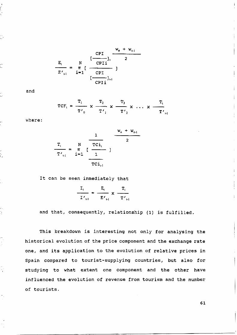
and

x x ---- x ... x T' 0 T' I T' 2 T't.1

where:

It can be seen inmediately that

= --- x I't_1 E't.) T't_1

and that, consequently, relationship (1) is fulfilled.

This breakdown is interesting not only for analysing the

historical evolution of the price component and the exchange rate

one, and its application to the evolution of relative prices in

Spain compared to tourist-supplying countries, but also for

studying to what extent one component and the other have

influenced the evolution of revenue from tourism and the number

of tourists.

61

(B) Relative prices in Spain compared to competitor countries )

from the Mediterranean area (PREe).

The countries providing tourist services, in competition )

I I

with Spain, which have been considered are:

- France

- Italy /!

I

- Greece

- Portugal

- Turkey

- Yugosla\:"ia

- Morocco

- Tunisia

I )! ,,v,

- Egypt

Let;

CPI t = consumer price index in Spain in t.

TC~ = number of pesetas per unit of currency of country i in t.

CPI~ = consumer price index of country i in t.

Wit = indicator of the relative importance of country i with

regard to countries competing with Spain in Mediterranean

area tourism.

"

/ I

I~ = annual data on revenue from tourism and trips, in

millions of dollars, corresponding to country i in the

year to which month t belongs.

i=l ..... N competitor countries indicated

62

!

') .-. ... I

I

c

Calculation of the weightings wb has been as follows:

:0 ,

Wit = N ~ lit

i=l

c As in the case of PREFtI a chained monthly index has been

built in the following manner:

\

C • \ r

PRECt = x--x-- x •.. x I l' ) I ' t-)!

where:

The breakdown in prices (P~) and exchange rates (TC~) is

, r, analagous to the one explained in above for relative prices f' v

compared to source countries.

The index has been constructed monthly, base 1983= 100, andc it has been aggregated quarterly by geometric means.

~c'

63

(C) Aggregate income of countries visiting Spain (INCOME)

since� quarterly accounting was not available, the number of )

countries considered in the construction of INCOME has been

reduced, leaving:

- Germany ,)

- France�

- United Kingdom�

- Holland�

- Sweden�

- U.S.A.�

- Italy�

Let:

; '..lYh =� indicator of real income of country i in the quarter

t, base 1983=100, obtained from the GDP or GNP series

(according to availability of information) at constant

1980 prices.

Wit =� relative importance in tourism in spain of country i

with regard to other countries visiting us. It has I

I

'] I -./ I

been calculated as in the case of PREF, but quarterly.�

i = 1 ... N source countries indicated in this section�

., The indicator of the evolution of aggregate real income in

the countries which traditionally visit us has been:

64

I '\,

, /,

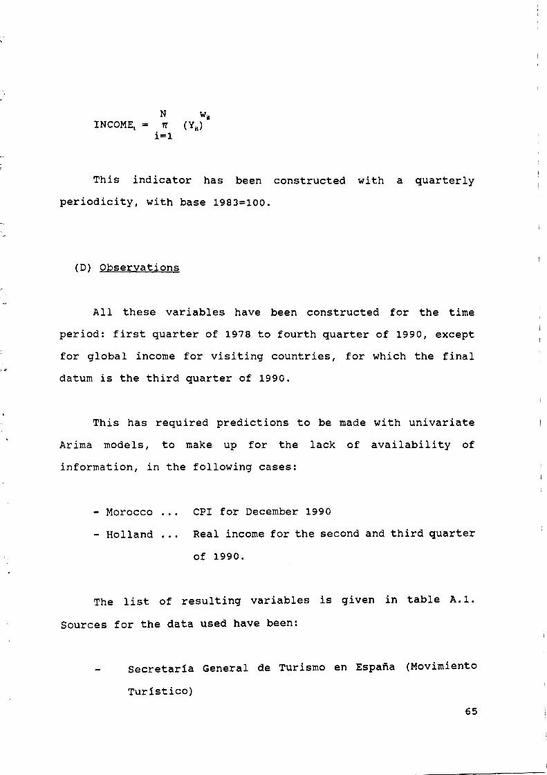
N Wit

INCOMEl = 1T (X'il) i=l

This indicator has been constructed with a quarterly

periodicity, with base 1983=100.

(D) Observations

All these variables have been constructed for the time

period: first quarter of 1978 to fourth quarter of 1990, except

for global income for visiting countries, for which the final ,"

datum is the third quarter of 1990.

This has required predictions to be made with univariate

Arima models, to make up for the lack of availability of

information, in the following cases:

- Morocco� CPI for December 1990

- Holland� Real income for the second and third quarter

of 1990.

The list of resulting variables is given in table A.l.

Sources for the data used have been:

Secretarla General de Turismo en Espana (Movimiento

Turlstico)

65

)Banco de Espana (Boletln Estadlstico)

World Tourist Organisation

O.E.C.D. (Main Economic Indicators)

I.M.F. (Balance of Payments, International Financial

statistics)

)

I )

.. '

66

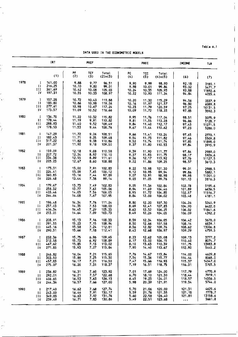
Table A.1

DATA USED IN THE ECONOMETRIC MODELS

IRT PREF PREC IMCOME TUR

(1) PF (2)

TCF (3)

Total (2)x(3>

PC (4)

TCC (5)

Total (4)x(5) (6) (7)

1978 I 11

III IV

141.00 216.25 361.69 197.31

9.88 10.10 10.42 10.55

9.77 9.80

10.08 10.33

96.51 99.01

105.03 108.97

9.90 9.98

10.24 10.22

9.99 10.01 10.35 10.90

98.90 99.84

105.93 111.34

92.18 93.32 93.88 94.84

3185.1 5471.7

11892.6 4055.4

, . 1979 I 11

111 IV

157.28 185.80 277.61 173.57

10.72 10.86 10.98 11.09

10.43 10.98 10.67 10.52

111. 88 119.26 117.24 116.66

10.20 10.16 10.23 10.09

11.30 11.97 11.79 11.72

115.29 121.57 120.59 118.33

94.56 96.80 97.25 97.85

3337.9 6089.8

10131.5 3592.3

(

1980 I 11

III IV

136.70 178.44 288.83 178.53

11.22 11.19 11.40 11.53

10.32 9.91 9.52 9.44

115.82 110.82 108.49 108.76

9.95 9.81 9.84 9.67

11.76 11.55 11.40 11.44

117.04 113.28 112.17 110.62

98.51 96.86 97.43 97.23

3075.9 5128.7

11271. 5 3286.0

1981 I 11

111 IV

147.29 182.43 317.22 201.37

11. 72 11.71 " .8211.92

9.26 9.35 9.38 9.18

108.51 109.48 110.86 109.50

9.66 9.54 9.52 9.37

11.41 11.73 11.74 11.80

110.24 111.82 111. 74 110.53

97.65 97.46 97.85 97.84

2770.1 5509.8

11898.0 3915.9

1982 1 11

111 IV

159.09 207.72 334.38 203.23

12.18 12.34 12.55 12.67

9.08 8.92 8.89 8.60

"0.58 110.10 111.61 108.88

9.39 9.37 9.36 9.22

11.90 11.93 12.17 11.86

111.77 111.75 113.92 109.35

97.84 98.17 97.76 98.37

2989.0 5926.6

11127.5 3613.3

1983 I 11

III IV

173.31 224.41 360.85 226.48

13.00 13.09 13 .16 13.44

7.91 7.65 7.44 7.38

102.83 100.12 97.89 99.14

9.22 9.12 9.07 9.03

10.98 10.95 10.91 11.05

101.30 99.94 98.98 99.76

99.01 99.86 99.98

101.13

2988.5 5882.1

11201.0 3816.3

1984 I 11

III IV

179.67 258.32 403.46 264.64

13.73 13.77 14.03 14.08

7.49 7.63 7.56 7.67

102.83 105.06 106.05 107.95

9.05 8.94 8.95 8.84

11.36 11.69 11.72 12.00

102.84 104.46 104.85 106.02

102.78 101.89 102.57 103.48

3195.6 6636.5

11516.7 4181.1

1985 1 11

III IV

196.48 257.03 406.34 253.05

14.34 14.35 14.45 14.64

7.76 7.53 7.29 7.09

111.24 108.03 105.33 103.73

8.80 8.69 8.63 8.49

12.20 12.41 12.32 12.26

107.30 107.83 106.25 104.05

104.26 104.90 106.02 106.09

3240.9 6422.0

11841.6 4392.2

1986 I 11

III IV

208.91 291.55 445.16 290.51

15.13 15.23 15.58 15.66

7.16 7.15 7.24 7.18

108.33 108.94 112.81 112.41

8.59 8.50 8.56 8.43

12.34 12.66 12.82 12.68

106.05 107.58 109.76 106.97

106.42 108.14 108.62 109.29

3678.0 6839.1

13006.8 4759.5

\'-'

1987 I 11

III IV

232.36 312.58 467.62 271.85

15.75 15.73 15.85 15.93

6.96 6.92 7.13 7.27

109.65 108.89 113.02 115.84

8.33 8.17 8.10 7.90

12.62 13.00 13.63 14.40

105.08 106.15 110.39 113.67

109.13 110.40 "'.75 112.90

3m.2 8074.7

13983.8 5445.2

1988 I 11

III IV

246.82 303.50 457.83 275.07

16.04 15.89 16.17 16.20

7.21 7.25 7.21 7.31

115.65 115.30 116.50 118.37

7.76 7.54 7.47 7.19

14.67 15.36 15.66 16.51

113.84 115.77 116.93 118.75

114.00 114.44 115.37 116.31

4629.8 8068.0

14547.0 5705.5

1989 I 11

III IV

236.82 292.01 406.65 244.36

16.31 16.21 16.53 16.57

7.60 7.57 7.63 7.66

123.92 122.68 126.13 127.00

7.01 6.70 6.45 5.98

17.69 18.10 19.23 20.39

124.00 121.30 124.01 121. 91

117.79 118.44 118.57 119.54

4770.9 7919.1

14356.5 5744.0

1990 I 11

111 IV

217.40 243.00 349.83 239.49

16.62 16.46 16.63 16.71

7.68 7.91 7.92 7.83

127.74 130.17 131.76 130.86

5.70 5.59 5.60 5.49

21.06 21.76 22.58 22.51

120.00 121.55 126.40 123.68

121.31 121.18 121.81

4625.6 m8.7

13158.6 5661.8