an econometric analysis of the tv advertising market ... › __data › assets › pdf_file › 0027...
TRANSCRIPT

Final report for Ofcom
An econometric analysis of the TV advertising market: final report
11 March 2010
Ref: 15880-275

Ref: 15880-275
Contents
0 Executive summary 1
1 Introduction 9 1.1 Background to the study 9 1.2 The UK TV advertising market 10 1.3 Objectives of the study 12 1.4 Structure of this report 12
2 Literature review 14
3 Data availability and channel groupings 16 3.1 Data used 16 3.2 Modelling period 25 3.3 Channel groupings 26
4 Approach to modelling the UK TV advertising market 28 4.1 The advertising demand model 28 4.2 The viewing demand model 39 4.3 Summary of approach 43
5 Results of the econometric analysis 45 5.1 Results from the advertising demand model 45 5.2 Results from the viewing demand model 55 5.3 Results from the robustness assessment 58 5.4 Summary of results 61
6 Conclusion 62
Annex A: Data sources used Annex B: List of channels Annex C: Further comparison between flexibilities and elasticities Annex D: Outputs from the econometric analysis Annex E: Analysis of policy options Annex F: Additional analyses Annex G: Robustness assessment

An econometric analysis of the TV advertising market: final report
Ref: 15880-275
Authors
Dr Mike Grant (Partner, Analysys Mason)
Mark Colville (Manager, Analysys Mason)
Marc Eschenburg (Consultant, Analysys Mason)
Sally Dickerson (Global Metrics Director, OmnicomMediaGroup, Global Managing Director, BrandScience)
Paul Sturgeon (Technical Director, BrandScience)
Neil Mortensen (Research Director, Omnicom Media Group)
Prof. Gregory Crawford (Professor, University of Warwick. Former Chief Economist at the FCC)
The authors would like to acknowledge the help and support of the Ofcom team.
In case of any queries on the contents of this report please contact either:
Mike Grant, Partner Analysys Mason Limited Bush House, North West Wing Aldwych London WC2B 4PJ UK Tel: +44 (0)20 7395 9000 Fax: +44 (0)20 7395 9001 [email protected]
Mark Colville, Manager Analysys Mason Limited St Giles Court 24 Castle Street Cambridge CB3 0AJ UK Tel: +44 (0)1223 460600 Fax: +44 (0)1223 460866 [email protected]
www.analysysmason.com
Registered in England No. 5177472
Confidentiality Notice: This document and the information contained herein are strictly private and confidential, and are solely for the use of Ofcom
Copyright © 2010. The information contained herein is the property of Analysys Mason Limited and its partners and is provided on condition that it will not be reproduced, copied, lent or disclosed, directly or indirectly, nor used for any purpose other than that for which it was specifically furnished.

An econometric analysis of the TV advertising market: final report | 1
Ref: 15880-275
0 Executive summary
This is the final report for Ofcom on the econometric modelling of the demand for TV advertising carried out by Analysys Mason, BrandScience and Professor Gregory Crawford. The report describes the methodology used, presents the results of our econometric analysis, and sets out the main conclusions from our work. We also provide analysis of several policy evaluation scenarios in the annexes. This study provides an analysis of the UK TV advertising market. Its aim is to conduct an econometric analysis which can be used by Ofcom as a tool in its regulatory decision-making process with respect to a change in the COSTA rules which define the maximum amount of advertising minutes allowed for public service broadcasters (PSBs) and non-PSBs.
One of the most distinguishing features of the TV advertising market is its two-sided nature (see Figure 0.1). On the one side, advertisers are buying airtime from broadcasters. On the other side, TV viewers are watching the programmes broadcast by the TV channels. In this market, advertising can be viewed as an implicit ‘price’ which viewers have to pay for consuming the content provided, and they will react to changes in the amount of advertising either by continuing to watch the same programme, switching to another channel, or switching off their TV.
Direct impact on supply of commercial
impacts
Demand and supply of commercial impacts
Direct impact on “price” paid by
viewers
Demand and supply of programming
Market 1: Advertising Market 2: Viewing
Ofcom
(COSTA rules)
Broadcasters ViewersAdvertisers
Direct impact on supply of commercial
impacts
Demand and supply of commercial impactsDemand and supply
of commercial impacts
Direct impact on “price” paid by
viewers
Demand and supply of programming
Demand and supply of programming
Market 1: Advertising Market 2: Viewing
Ofcom
(COSTA rules)
Broadcasters ViewersAdvertisers
Figure 0.1: The two-sided nature of the UK TV advertising market
We have reflected this double aspect of the market by developing two models:
• Advertising demand model: This looks at the demand and supply for advertising by advertisers and broadcasters. Given the dynamics of the TV advertising market, we have used an inverse demand framework to understand key dependencies between the price of

An econometric analysis of the TV advertising market: final report | 2
Ref: 15880-275
advertising and variables such as the quantity of impacts supplied, the share of commercial impacts (SOCI) of a channel, or external factors such as the prevalence of Internet advertising.
• Viewing demand model: Changing the COSTA rules implies new rules on the maximum number of advertising minutes broadcast. Advertising is seen as an implicit price paid by audiences to watch TV content, and so changes to the COSTA rules will impact the number of people watching a specific programme, and should be taken into account when evaluating the impact of regulatory changes. Our viewing demand model therefore estimates the reaction of viewers to a change in advertising minutes as a consequence of changes in the advertising rules.
Given the size and importance of advertising in the economy, there is a relatively low volume of academic work covering the topic. A primary reason for this scarcity is the difficulty in obtaining the data necessary to estimate advertising demand. Viewership, advertising minutes and advertising prices (as well as ancillary information about programming characteristics, viewer demographics and advertiser characteristics) are all needed in order to accurately model advertising demand. However, although viewership and advertising minutes are typically available from TV ratings organisations such as Nielsen in the USA and BARB in the UK, the prices paid by advertisers (or their ad agencies or media buyers) are typically commercially sensitive, and only some information is available on quarterly pricing for some of the major advertising sales houses.
Our study attempts to address some of these difficulties and thereby contribute to an improved understanding of the TV advertising market. Our model is broadly based on the approach taken by Wilbur (2008), but additionally uses more detailed data. With regard to the improvements in the data available to us:
• We have gained access to proprietary information from the Omnicom Media Group (OMG), and in particular can draw on monthly advertising pricing data on a channel-by-channel level. Given the seasonality of TV viewing (and hence advertising prices), this increased granularity of the data (compared to quarterly data on an industry level available in the public domain) constitutes a significant improvement over previous studies and allows us to address one of the major gaps in the academic literature.
• In addition, our use of extensive UK databases of viewership and advertising minutes (a combination of data available through BARB and in-house data from OMG) has allowed for very detailed viewing analyses, and provide a further improvement over previously available datasets.
Given the differentiation in COSTA rules between PSBs and non-PSBs on the one hand, and the significant differences between PSB channels on the other hand, we have defined a total of seven channel groupings which we have incorporated into our modelling framework.1
1 ITV1, C4, Five, Non-PSBs/Rest of the market, channels in ITV portfolio, C4 portfolio, and Five portfolio. These are shown as part of
our first results table in
Figure 0.3 below (page 5).

An econometric analysis of the TV advertising market: final report | 3
Ref: 15880-275
Based on the two-sided nature of the advertising market, the available data and existing TV advertising regulation, we have developed the final model specifications. The key characteristics of these model specifications are summarised in Figure 0.2 below.
Advertising demand model Viewing demand model
Underlying economic model Inverse demand system Logit market share model
Econometric method Ordinary Least Squares (OLS) Ordinary Least Squares (OLS)
Cross-equation restrictions Seven individual equations Four individual equations
Sample size 79-90 (depending on equation) 7540 – 198 583 (depending on equation)
Period under evaluation January 2002 – August 2009 January 2009 – June 2009
Applied time unit Month 30-minute blocks across the day
Dependent variable Cost per thousand (CPT) for an individual channel or a channel family
Market share of a programme
Independent variables Quantity of commercial impacts supplied by channels
Length of advertising break
Monthly lags of cost per thousand Programme (dummy)
Share of Commercial Impacts (SOCI) Hour of day (dummy)
Monthly dummy variables Month (dummy)
Online page impressions
FTSE index
Figure 0.2: Overview of key characteristics of the advertising and viewing demand models
Ofcom’s primary concern is to understand the effects of changes to the COSTA rules on advertising revenue streams. Rule changes are likely to result in a change in advertising minutage, and therefore the supply of impacts, by (at least some) channels. This will in turn directly affect the market prices for advertising impacts. The goal of our advertising demand model is therefore to capture the dynamics of supply and demand for TV advertising. The main outputs we have derived from this analysis are the own-price inverse elasticity and the cross-price inverse elasticity of TV advertising demand, for the seven channel groupings.2
In order to derive the relevant price inverse elasticities, we have used an ordinary least squares (OLS) approach. In Section
4.1 we justify in detail the use of this comparatively simple approach in the context of the UK TV advertising market. We have also run various robustness tests to support our assumption of perfectly inelastic supply, confirm the validity of our baseline OLS approach, and guard against endogeneity at the disaggregated level. The instrumental variables used and other details of these checks are discussed in Section 4.1.4.
2 See Section 4.1.2. Inverse elasticities describe the change in the price for advertising on channel i following a change in the supply
of commercial impacts either on the same channel i (own-price inverse elasticity), or on another channel j (cross-price inverse elasticity).

An econometric analysis of the TV advertising market: final report | 4
Ref: 15880-275
Given the dynamics in most economic markets, traditional economic analysis usually reports demand elasticities estimating how a change in price affects the demand for a good. However, demand elasticities are derived using a regular demand relationship. In our model, we relied on an inverse demand relationship, regressing the price for advertising on the quantity of impacts in the market. Based on our understanding of the advertising market, we feel that this is the most appropriate mechanism. Broadcasters select the quantities of commercial impacts supplied in the advertising market, with prices adjusting following a change in supply. Hence, the price for advertising is the adjusting mechanism following a change in the (fixed) supply of commercial impacts, and we are primarily interested in estimating this change in price following a change in the supply of commercial impacts.
Because we use an inverse demand framework, instead of elasticities we derive what are known in the technical literature as flexibilities. Flexibilities describe the change in the price for advertising on channel i following a change in the supply of commercial impacts either on the same channel i (own-price flexibility) or on another channel j (cross-price flexibility). This technical use of the term ‘flexibility’ may be unfamiliar to the general reader, although it is common in economics literature discussing the agricultural and natural resources sectors.3
The main outputs derived from our advertising demand model are own- and cross-price inverse elasticities for advertising for all seven channel groupings. We initially tested a model specification which included the quantities of all seven groupings in each equation. However, we were unable to derive significant results and therefore had to restrict our analysis to the main PSB flagship channels and the corresponding respective channel families. The parameters for the PSB ‘portfolio channels’, as depicted below were derived through a process of ‘backing out’ as described in Section
In order to avoid possible misunderstanding, in this report we refer to flexibilities by what we believe is the more intuitive term ‘inverse elasticities’.
5.1. Figure 0.3 presents a matrix summarising the estimated short-run inverse elasticities.4
3 See Park and Thurman (1999) and the references cited there.
4 Note that these figures represent point estimates and are therefore subject to standard errors.

An econometric analysis of the TV advertising market: final report | 5
Ref: 15880-275
ITV1 C4 Five Non PSBs
ITV Portfolio channels
C4 Portfolio channels
FIVE Portfolio channels
ITV1 -1.05 - -0.43 - - - -
C4 -0.41 -0.88 - -0.34 - - -
Five 0.28 - -0.75 0.32 - - -
Non PSBs -0.20 -0.18 - -1.10 - - -
ITV Portfolio channels
- - - - -0.14 - -
C4 Portfolio channels
- - - - - -0.45 -
FIVE Portfolio channels
- - - - - - 0.04
Figure 0.3: Summary of price inverse elasticities [Source: Analysys Mason, BrandScience]
In the matrix above we have only shown inverse elasticities for which the relevant coefficient of the regression analysis was significant at the 10% level In Figure 0.4 below we show the 95%confidence intervals surrounding these short-run own and cross-price inverse elasticities for the four main channel groupings.
ITV1 C4 Five Non-PSBs
ITV1 [ -1.361 : -0.736 ] - [ -0.678 : -0.172 ] -
C4 [ -0.628 : -0.185 ] [ -1.086 : -0.679 ] - [ -0.591 : -0.08 ]
Five [ 0.025 : 0.537 ] - [ -1.145 : -0.363 ] [ 0.041 : 0.602 ]
Non-PSBs / Rest of the market
[ -0.409 : 0.012 ] [ -0.384 : 0.019 ] - [ -1.388 : -0.809 ]
Figure 0.4: 95% confidence intervals surrounding short-run own and cross-price inverse elasticities
[Source: Analysys Mason, BrandScience]
The inverse elasticities describe the change in the price for advertising following a change in the supply of commercial impacts. For example the first cell in Figure 0.3 indicates that an increase in the supply of impacts on ITV1 by 1% would result in a -1.05% change in the price per impact for ITV1. Reading further along the row the same 1% increase in ITV1 impact supply would result in a -0.43% change in the price per impact on Five.
Our results indicate that the own-price inverse elasticities are generally higher than any cross-price inverse elasticities, and are negative for all channels save for the ‘Five portfolio channels’ grouping. The fact that for ITV1 and the non-PSBs the own-price inverse elasticities are larger than 1 indicates that demand is inelastic, which means that a 1% increase in impacts will lead to more than a 1% decrease in prices, and therefore result in lower revenues.

An econometric analysis of the TV advertising market: final report | 6
Ref: 15880-275
The viewing demand model estimates the reaction of viewers to a change in the advertising minutes provided. The main output we derive from this model is the viewing demand elasticities, which measure the reaction of viewers to a change in advertising minutes. (Note that, unlike the advertising demand model, in the context of the viewing demand model we talk about regular elasticities rather than inverse elasticities.)
The viewing demand model evaluates the change in market share that occurs between two episodes of the same programme. As highlighted in Section 3.1.3, the data available to us has shown that there is significant variation in the advertising minutes between shows, enabling such an evaluation. (It is important to note that the concept of market share used in our model implicitly takes into account the option of not viewing TV at all.) We have used an OLS logit model to estimate viewing demand elasticities. This model, and the robustness assessment carried out on our baseline specification, are described in Section 4.2.2. The calculated viewing demand elasticities are shown in Figure 0.5.
Viewing elasticity (off-peak)
Viewing elasticity (peak)
Figure 0.5: Summary of
viewing demand
elasticities [Source:
Analysys Mason,
BrandScience]
ITV1 -0.0022 -0.0041
C4 -0.0010 -0.0016
Five -0.0010 -0.0010
ITV portfolio channels -0.0004 -0.0013
C4 portfolio channels -0.0002 -0.0009
Five portfolio channels -0.0002 -0.0007
Non-PSBs -0.0003 -0.0013
Figure 0.6 below shows 95% confidence intervals surrounding these viewing demand elasticities.
95% confidence interval surrounding viewing demand elasticity (off-peak)
95% confidence interval surrounding viewing demand elasticity (peak)
Figure 0.6: 95%
confidence intervals
surrounding viewing
demand elasticities
[Source: Analysys
Mason, BrandScience]
ITV1 [ -0.0025 : -0.0018 ] [ -0.0054 : -0.0027 ]
C4 [ -0.0011 : -0.0008 ] [ -0.0021 : -0.001 ]
Five [ -0.0011 : -0.0008 ] [ -0.0014 : -0.0007 ]
ITV portfolio channels [ -0.0005 : -0.0004 ] [ -0.0015 : -0.0012 ]
C4 portfolio channels [ -0.0003 : -0.0002 ] [ -0.0009 : -0.0008 ]
Five portfolio channels [ -0.0002 : -0.0002 ] [ -0.0008 : -0.0007 ]
Non-PSBs [ -0.0003 : -0.0003 ] [ -0.0014 : -0.0012 ]
In Figure 0.5 above the first cell, by way of example, means that a 1% increase in advertising minutage on ITV1 at peak times would result in a 0.002% decrease in viewing demand for

An econometric analysis of the TV advertising market: final report | 7
Ref: 15880-275
programming on that channel. In a manner similar to the price inverse elasticities for advertising demand, the viewing demand elasticities are negative, indicating that an increase in the number of advertising minutes reduces the market share of a programme.
Our results show that viewing elasticities vary significantly between channels and periods. For example, ITV1’s viewing is by far the most elastic during peak and off-peak times. However, the elasticity is significantly higher in peak times, perhaps reflecting the greater choice of high-quality alternative programming that is available during these times.
Overall though, the main observation from these results is that the viewing elasticities are very low for all channels at all times. This means that the quantity of advertising minutes does not significantly affect viewer behaviour. (We note in passing that this is, of course, a separate issue from how advertising affects the surplus a consumer derives from watching a programme: this surplus is likely to be reduced by increases in the amount of advertising.)
The overall conclusions which can be drawn from our econometric analysis are that:
• Demand for advertising appears to be flexible (i.e. inelastic). This implies that an increase in the supply of commercial impacts will be likely to lead to a relatively larger fall in the prices for impacts and visa versa.
• Demand for programming by viewers is highly inelastic, and changes in advertising minutage do not lead to substantial changes in viewing habits.
Using our results, we have conducted a scenario-based evaluation of several policy options which we consider may be of interest to Ofcom. We have defined four scenarios, which are compared against a base case. Further details of this scenario-based analysis are provided in Annex E.

An econometric analysis of the TV advertising market: final report | 9
Ref: 15880-275
1 Introduction
This is the final report for Ofcom on the econometric modelling of the demand for TV advertising carried out by Analysys Mason, BrandScience and Professor Gregory Crawford. The report describes the methodology used, presents the results of our econometric analysis, and sets out the main conclusions from our work. We also provide analysis of several policy evaluation scenarios in the annexes.
1.1 Background to the study
As a result of its review of advertising regulation, Ofcom introduced the Code on the Scheduling of TV advertising (COSTA) on 1 September 2008, replacing the previous Rules on the Amount and Distribution of Advertising (RADA).5 The COSTA rules define a revised framework concerning advertising and teleshopping for two categories of TV channels. ITV1, Channel 46 and Five are defined as public service broadcasters (PSBs), while all remaining channels, including smaller channels from the PSB channel families (e.g. ITV2 or E4) are termed non-PSBs. Those COSTA rules which are particularly relevant to our study concern the maximum advertising minutage7
Ofcom further states in its decision on the new code for advertising that it intends to review the COSTA rules in Spring 2010. In particular, it wishes to evaluate the impact of “harmonising up” or “harmonising down” the advertising minutage allowed to PSBs and non-PSBs as defined in 2008. This process of harmonisation would create a level playing field with regard to the maximum amount of advertising minutes allowed in each hour. Harmonising up would allow an average of 9 minutes of advertising per hour for all channels (as in the current non-PSB rules) whilst harmonising down would allow an average of 7 minutes per hour (8 minutes in peak) for all channels (current PSB rules). Ofcom also states that it might consider alternative regulatory options.
allowed in peak hours (between 6pm and 11pm every day) and during off-peak hours to channels in both categories of channel. For PSBs, a maximum of 168 minutes per day are allowed, i.e. an average of 7 minutes per hour. For peak hours, an average of 8 minutes per hour is allowed over the 5 hour peak period, and within any specific hour the total must not exceed 12 minutes. Moreover, PSBs are required to sell all of their advertising airtime. In contrast, non-PSBs can sell up to an average of 9 minutes per hour, with a maximum of 12 minutes in any individual hour. Ofcom’s rules do not distinguish between peak and off-peak periods for non-PSBs.
5 http://www.ofcom.org.uk/consult/condocs/rada08/statement/
6 In addition, S4C which replaces Channel 4 across Wales has been defined as a PSB by Ofcom. Within our analysis, we do not explicitly differentiate between these two channels. We treat both channels together as “Channel 4”.
7 Defined as the maximum number of minutes of advertising permitted per hour of broadcast

An econometric analysis of the TV advertising market: final report | 10
Ref: 15880-275
Following the 2003 merger between the two sales houses for ITV airtime, Carlton and Granada, in January 2004 the Competition Commission had put in place the Contract Rights Renewal (CRR) framework. The CRR provides a rollback option for advertisers contracting with ITV to sign share deals for “Regional Channel 3 services” on the same contractual basis as in 2003.
The aim of our study is to contribute to Ofcom’s process of revising the COSTA rules by developing a rigorous econometric model of the UK TV advertising market. This report thereby aims to assist Ofcom in its regulatory decision making process, and to provide some of the relevant tools for an in-depth quantitative assessment of various potential regulatory remedies which are at Ofcom’s disposal.
1.2 The UK TV advertising market
In the TV advertising market, advertisers are placing advertisements on TV programmes to advertise products by reaching a previously defined target audience (usually specified by a certain demographic group). In order to reach this audience, advertisers buy airtime from channel-specific advertising sales houses. The key trading unit in this sales process which determines the reach and effectiveness of a campaign is called the commercial impact. Commercial impacts are defined as the number of individual viewings of a single advertising spot. Advertisers commit an overall budget to a campaign in exchange for the delivery of a target number of commercial impacts in a certain demographic over a fixed period of time. As the precise number of commercial impacts cannot be influenced by the broadcasters,8
This process of placing adverts and achieving commercial impacts involves three main market players – advertisers, broadcasters and viewers. All these players have different incentives and interests which need to be taken into account in an analysis of the TV advertising market.
the actual price per impact – termed cost per thousand impacts (CPT) or station average price (SAP) is only calculated retrospectively as a benchmark for future campaigns.
Figure 1.1 illustrates the interrelation between these three types of players.
8 Small variations in the number of commercial impacts can occur if a programme over- or under-performs in terms of the audience it
reaches for the target demographic.

An econometric analysis of the TV advertising market: final report | 11
Ref: 15880-275
Broadcasters Viewers
AdvertisersAccess point to potential
customers
Main source of income
Source of income
Source of entertainment
Advertising audience
Product information
Broadcasters Viewers
AdvertisersAccess point to potential
customers
Main source of income
Source of income
Source of entertainment
Advertising audience
Product information
Figure 1.1: Interaction between the main types of players in the advertising market
This complex interaction, with broadcasters effectively representing an intermediary between advertisers and viewers, has led to a “two sided” market for TV advertising. In the context of this study, the two-sided nature of the TV advertising market implies that changing the COSTA rules will affect two separate but interlinked markets:
• On the one side, advertisers are buying airtime from broadcasters. Any changes made to the COSTA rules affecting advertising minutage will directly affect the number of commercial impacts which can be supplied by channels. In that respect, our econometric analysis derives the price inverse elasticity9
• On the other side, TV viewers watch those programmes broadcast by the TV channels. Advertising can be viewed as an implicit “price” which viewers have to pay for consuming the content provided. Viewers will react to changes in the amount of advertising by either continuing to watch the same programme, switching between channels, or switching off. As a result, the effect of any change in the supply of commercial impacts through a change in the COSTA rules concerning advertising minutes is muted by the viewer’s decision on how much content to consume. In our model, we control for this effect by introducing a model of viewing demand that calculates the elasticity of demand for programming from viewers.
of advertisers for audiences, to understand how broadcasters’ revenues are affected by changes in supply.
9 It is standard economic practice to talk about “demand elasticities”, a term which describes the change in equilibrium quantity
following a change in the price for a product. Given the mechanics of the advertising market, where prices react to a change in the quantity of commercial impacts supplied, we have used an inverse demand relationship in our model. This has led us to use ‘inverse elasticities’ describing the change in the price for advertising following a change in the quantity of commercial impacts supplied. Our approach to deriving inverse elasticities is explained in more detail in Section 4.1.2.

An econometric analysis of the TV advertising market: final report | 12
Ref: 15880-275
Figure 1.2 below illustrates the two-sided nature of the advertising market and the impact of the COSTA rules.
Direct impact on supply of commercial
impacts
Demand and supply of commercial impacts
Direct impact on “price” paid by
viewers
Demand and supply of programming
Market 1: Advertising Market 2: Viewing
Ofcom
(COSTA rules)
Broadcasters ViewersAdvertisers
Direct impact on supply of commercial
impacts
Demand and supply of commercial impactsDemand and supply
of commercial impacts
Direct impact on “price” paid by
viewers
Demand and supply of programming
Demand and supply of programming
Market 1: Advertising Market 2: Viewing
Ofcom
(COSTA rules)
Broadcasters ViewersAdvertisers
Figure 1.2: The two-sided nature of the UK TV advertising market
1.3 Objectives of the study
The objectives of this study are therefore to:
• develop a robust methodology for an econometric analysis of the UK TV advertising market reflecting the two-sided nature of the TV advertising market
• carry out this econometric analysis and thereby estimate the impact that changing the rules concerning advertising minutage will have on the broadcaster’s ability to supply and charge for particular programme audiences
• develop this analysis further with a scenario-based policy evaluation which simulates the expected effects of changes in the COSTA rules on the advertising revenue streams in the UK TV market over a defined period of time
1.4 Structure of this report
The remainder of this document is structured as follows:
• Section 2 gives a short overview of the relevant academic literature in this field and positions our study within this set of publications.
• Section 3 summarises the available data as well as the channel groupings that were used for the modelling.

An econometric analysis of the TV advertising market: final report | 13
Ref: 15880-275
• Section 4 develops our methodology for the econometric analysis of the UK TV advertising market and specifies the relevant equations used in our advertising and viewing demand model.
• Section 5 provides the results of our econometric analysis.
• Section 6 summarises the main conclusions of this study.
The report also contains several Annexes:
• Annex A summarises the data sources we have drawn upon during our analysis.
• Annex B provides information on sales houses and channel groupings.
• Annex C explains the differences between inverse and regular demand systems.
• Annex D provides details of the outputs from our econometric analysis.
• Annex E discusses our scenario-based evaluation of changes in the COSTA rules.
• Annex F provides examples of some of the analysis carried out to derive coefficients and elasticities.
• Annex G provides details of the robustness assessments used.

An econometric analysis of the TV advertising market: final report | 14
Ref: 15880-275
2 Literature review
While there are volumes of academic literature analysing the impact of advertising on consumer behaviour,10 there is surprisingly little recent academic work analysing the demand and supply of advertising by advertisers.11 Goettler (1999) and Wildman, McCullough and Kieschnick (2004)12 estimate reduced-form relationships of the responsiveness of advertising prices to audience size, but do not estimate the demand for audiences. Bel and Domenech (2008) and Wilbur (2008)13 are notable exceptions. Bel and Domenech (2008) relate advertising prices to advertising minutes and channel audiences in the Spanish TV market, but unfortunately do not account for the possible endogeneity of either variable. Wilbur (2008) is notable, both for explicitly modelling both sides of the TV market (i.e. the demand for programming by households and the demand for audiences by advertisers) and for estimating aggregate advertiser demand for those audiences.14
Given the size and importance of advertising in the economy, this relatively low volume of academic work may seem surprising. A primary reason for this scarcity is the difficulty in obtaining the data necessary to estimate advertising demand. Viewership, advertising minutes, and advertising prices (as well as ancillary information about programming characteristics, viewer demographics, and advertiser characteristics) are all needed in order to accurately model advertising demand. However, although viewership and advertising minutes are typically available from TV ratings organisations such as Nielsen in the USA and BARB in the UK (see our table of data sources in Section
In both exercises, care is taken to account for potential endogeneity of viewership, advertising minutes, and/or advertising prices in the estimation. While the focus of Wilbur’s paper is limited to aggregate demand for advertising on US broadcast TV networks, the basic framework can be extended to allow for multiple channels, differentiated broadcasters (i.e. PSBs and non-PSBs), and advertising limits of the kind enforced by COSTA.
3.1), the prices paid by advertisers (or their ad agencies or media buyers) are typically considered sensitive,
10 Bagwell, K., “The Economic Analysis of Advertising,” in M. Armstrong and R. Porter, eds., Hand-book of Industrial Organization, Vol.
3, North-Holland, 2007, pp. 1701–1 844
11 Older work includes Hendry, David F., “An Econometric Analysis of TV Advertising Expenditure in the United Kingdom,” Journal of Policy Analysis, 1992, 14 (3), 281–311, Masih, R., “An Empirical Analysis of the Demand for Commercial TV Advertising,” Applied Economics, 1999, 31, 149–163, Goettler, R., “Advertising Rates, Audience Composition, and Competition in the Network Television Industry,” 1999. mimeo, Carnegie-Mellon University, and Ofcom’s previously commissioned study on this topic, PricewaterhouseCoopers, “Economic Analysis of the TV Advertising Market,” Technical Re-port, PricewaterhouseCoopers December 2004.
12 Wildman, S., B. McCullough, and R. Kieschnick, “The Market for Television Ad Time: Model and Evidence,” 2004. mimeo, Center for the Analysis of Property Rights and Innovation (CAPRI).
13 Bel, Germa and Laia Domenech, “What Influences TV Advertising Price? An Empirical Analysis on the Spanish Market,” 2008. forthcoming, Journal of Media Economics; Wilbur, Kenneth C., “A Two-Sided, Empirical Model of Television Advertising and Viewing Markets,” Marketing Science, 2008, 27 (3), 356–378.
14 In recent work, Wilbur, Goeree and Ridder (2009) extend the analysis in Wilbur (2008) to consider a more general demand structure and the effect of product placements on viewership.

An econometric analysis of the TV advertising market: final report | 15
Ref: 15880-275
competitive information and only some information is available on quarterly pricing data for some of the major advertising sales houses.
Our study attempts to address some of the shortcomings identified in the academic literature and thereby contribute to an improved understanding of the TV advertising market. Our model is broadly based on the approach taken by Wilbur (2008), but additionally uses more detailed data and takes into account several factors that are very different between the two markets under evaluation (US and UK).
With regard to the improvements in the data available to us:
• For the purpose of this study, we have gained access to proprietary information from the Omnicom Media Group (OMG). In particular, we can draw on monthly advertising pricing data on a channel-by-channel level. Given the seasonality of TV viewing (and hence advertising prices), this increased granularity of the data (compared to quarterly data on an industry level available in the public domain) constitutes a significant improvement over previous studies and allows us to address one of the major gaps in the academic literature.
• In addition, extensive UK databases of viewership and advertising minutes (a combination of data available through BARB and in-house data from OMG) have allowed for very detailed viewing analyses, and provide a further improvement over previously available datasets.
Regarding the second point (differences between the UK and US markets), the institutional rules in the UK suggest exogenous impacts:
• In the UK, PSBs are required to sell all their advertising minutes.
• The role of PSBs in the UK is significantly more pronounced than that of such broadcasters in the USA.
• In the UK, the BBC competes for audiences (and therefore for content) with other stations but, due to the regulatory framework in place, derives its funds through TV licence fees and is therefore not allowed to compete for advertising with other UK broadcasters.
• The Wilbur US-based study focussed solely on market interactions within the TV advertising market – our study is not constrained in this way and considers substitution effects with advertising platforms on other media.
We expect that our report may also stimulate a number of follow-on studies in other countries which could create a wider evidence base in the academic literature, facilitate international comparisons, and foster an improved understanding of the mechanics of the TV advertising market from an international perspective.

An econometric analysis of the TV advertising market: final report | 16
Ref: 15880-275
3 Data availability and channel groupings
Figure 1.1 illustrates the two-sided nature of the TV advertising market. In order to appropriately model this market and capture the mechanics underlying the interaction between viewers, advertisers and broadcasters, we have developed two independent models accounting for both sides of this market:
• an advertising demand model which models the (inverse) demand for commercial impacts by advertisers, by evaluating the effect of the volume of impacts on the price of impacts
• a viewing demand model which models the demand for programmes by viewers, and assesses the impact of broadcast advertising minutes on the amount of programme viewing.
As discussed in Section 2, one of the main issues faced by previous publications was the lack of availability of relevant data points. It is therefore important to understand how we have determined the final model specification based on the data available to us, the opportunities it offered and the constraints it imposed. This section discusses the data we have used, and is divided into three main sub-sections as follows:
• Data used – an overview of major data sources and inputs to the model.
• Modelling period – the appropriate time horizon for our analysis, which is dependent on the available data but also on recent market and regulatory trends in the TV advertising industry.
• Channel groupings – sufficiently granular channel groupings are important to conduct a thorough analysis of the impact of changes in the COSTA rules on advertising revenue streams within the TV industry.
3.1 Data used
We here provide relevant information for an evaluation of the main data sets underlying our econometric analysis. More specifically, we
• list the different data series used and the sources for this data • provide an overview of the available revenue data which has been used, • describe our findings from an analysis of the advertising minutage data • introduce the share of commercial impacts (SOCI) as an important parameter in our analysis • list potential demand shifters for the advertising model.
3.1.1 Data overview
As part of Omnicom Media Group (OMG), BrandScience has been able to draw on a wide range of relevant data for this study. In particular, we have been able to collect revenue data allowing for

An econometric analysis of the TV advertising market: final report | 17
Ref: 15880-275
a monthly split of revenue by channel. This allows us to develop unique insights compared to previous analyses which could only draw on revenue data available in the public domain. Figure 3.1 below provides a summary of the key data series used in the main models. We provide a more extensive list in Annex A: covering all the data sets which have been taken into account while developing the model and forecasts (but which might not have made their way into the final specification).
Variable Frequency Period available Source Used in…
Television
Individual station spot impacts Monthly (by demographic)
01/02 – 07/09
BARB/OMG Advertising model
Individual station spot impacts Commercial break by minute
01/09 – 07/09 BARB/OMG Viewing model
Individual station spot lengths Commercial break by minute
01/09 – 07/09 BARB/OMG Viewing model
Individual station programme TVRs*
Programme 01/02 – 07/09 BARB/OMG Advertising model
Individual station sponsorship impacts
Quarterly 01/02 – 07/09 BARB/OMG Advertising model
Individual station prices Monthly (by demographic)
01/02 – 07/09 OMG Advertising model
Other media
Total internet page impressions
Monthly 01/02 – 07/09 Comscore/ Nielsen/ OMG
Advertising model
Macroeconomic/external
FTSE Monthly 01/02 – 07/09 Reuters Advertising model
Major events – UK Monthly 01/02 – 07/09 BrandScience Advertising model
Major events – World Monthly 01/02 – 07/09 BrandScience Advertising model
Weather Monthly
Daily
01/02 – 07/09
01/07 – 07/09
Met Office
Met Office
Advertising model
Market size/technology/other
Legislative change affecting Advertising sector sizes
Monthly 01/02 – 07/09 BrandScience Advertising model
* TVRs – Television Viewer Ratings
Figure 3.1: Summary of key data used in the development on the advertising and viewing demand
model [Source: BrandScience]

An econometric analysis of the TV advertising market: final report | 18
Ref: 15880-275
As mentioned earlier, a common benchmark of prices in the advertising market is the cost per thousand impacts (CPT). For the purpose of our models, we derive this data by dividing monthly revenue for a channel by the number of impacts provided. This is analogous to calculations used within the advertising industry. The CPT is not an explicit price which is agreed in advance: negotiations are actually based on a target number of commercial impacts against which a fixed spend per campaign is agreed. As the precise number of impacts cannot be foreseen, broadcasters and TV buyers aim to deliver as close to the target number of impacts as possible, and the exact CPT is calculated ex post facto and forms a benchmark for future negotiations. Should the actual delivery of commercial impacts for a campaign differ significantly from the previously agreed target, compensation schemes are put into place to practically arrive at the implicitly agreed CPT.
In order to ensure a robust econometric analysis, the collected data has been formatted and tested. All data has been cleaned and checked for potential errors and outliers, and we have conducted a range of accuracy assessments. As a result, we are confident that it is appropriate to use the collected data for the purpose of our modelling.
3.1.2 Advertising revenue data
TV advertising revenue data is only readily available in the public domain at a quarterly frequency, and only at a broadcast level. This data is supplied by the Advertising Association and although it is a good indicator of top-line trends, it does not have the required sensitivity, accuracy and depth needed for this type of analysis. Our study utilises actual monthly data held by OMG, which possesses accurate monthly data from 2002 onwards, split out by major channels and sales houses. Following standard practice, we have deflated the data using a price index. We have used the headline inflation measure (RPIX)15
Figure 3.2 at the start of the modelling period, and we have re-based
so that figures are at 2002 real-term prices. gives an indication of the price trend over the period modelled (exact prices are redacted in order to maintain commercial confidentiality).
15 Retail prices index (RPI) excluding mortgage interest payments.

An econometric analysis of the TV advertising market: final report | 19
Ref: 15880-275
Jan-02 Jan-03 Jan-04 Jan-05 Jan-06 Jan-07 Jan-08 Jan-09
Cos
t per
thou
sand
(GB
P)
ITV1 C4 Five Sky-Non
Figure 3.2: Real January 2002 advertising prices for main channel categories [Source: OMG, 2009]
3.1.3 Advertising minutage data
We have gathered advertising minutage data at both aggregated and disaggregated levels. At the aggregate level, we consider the total advertising minutes broadcast by a channel in a monthly period. At a more disaggregated level, we consider data on the length of each individual commercial break during each programme across a representative sample of 28 channels This data is used in our viewer demand model in combination with minute-by-minute data on the number of viewers for a given programme.
Overall commercial minutage
Our analysis assesses the impact of changes in the rules regarding the permitted number of advertising minutes upon the net advertising revenue of individual stations. The approach is based upon the assumption that a change in the rules regarding the number of commercial minutes allowed actually results in a change in the amount of commercial minutage on TV.
An individual station consistently selling all available inventory is likely to increase the amount of commercial minutage if the rules allow this. The same station will be forced to sell less inventory if the opposite decision is made and a greater restriction is placed upon the amount of commercial minutage. However, if a station is not selling all available inventory, the effects are less clear. A station that is either unwilling or unable to sell all its inventory could be unaffected by a change in the rules regarding the amount of commercial minutes.

An econometric analysis of the TV advertising market: final report | 20
Ref: 15880-275
PSBs are under an obligation to sell all advertising minutes. Non-PSBs are not, although we assume that the non-PSB stations do utilise all of the available inventory – an assumption which is supported by our analysis of the data. Figure 3.3 shows that the available data on average daily advertising minutes by channels confirms our assumptions.
0
50
100
150
200
250
ITV1 C4 FIVE ITV3 E4 DISC MTV2 DAVE
Adv
ertis
ing
min
utes
per
day
Average daily minutes Maximum allowance (PSBs)
Maximum allowance (non-PSBs)
Figure 3.3: Daily number of broadcast advertising minutes by channel [Source: BARB/OMG]
The sample above covers average daily minutes in 2009. The sample may show slight deviations from the maximum permitted airtime due to channels not broadcasting 24 hours or the coverage of breaking news. Overall, though, we consider that there is strong evidence supporting our assumption that non-PSBs sell all available inventory.
This is further supported by the incentives created by the introduction of the Contract Rights Renewal (CRR) framework in 2004. TV airtime has historically been negotiated using a simple mechanism whereby broadcasters are often rewarded for audience improvements with a higher share of revenue commitment from clients and agencies. This basic relationship did not always hold true, however, as ITV1 often negotiated more revenue share than the audience it delivered would normally suggest – delivering a premium and therefore reducing the reward smaller channels could achieve through audience growth. It was felt that this could lead smaller channels to attempt to manipulate their airtime to improve yield in the face of no guaranteed increases in volume from annual negotiation.
CRR immediately changed the focus of the negotiation round. For the first time it legalised the relationship between revenue and audience. Advertisers and agencies were no longer under pressure from ITV1 to over-deliver for fear of losing (for example) access to quality programmes and particular day-parts. Each year there were now share gains to be had, as ITV1 (in decline due

An econometric analysis of the TV advertising market: final report | 21
Ref: 15880-275
to multi-channel penetration increases) began to lose audience and the power to ‘make’ the market continue to invest in ITV1. This made it an absolute imperative for all broadcasters to maximise delivery of commercial impacts to increase the level of revenue advertisers were now able to invest without detrimental effects to their overall TV campaigns. Essentially the fall in ITV1’s share of impacts entailed a lower revenue share for ITV1 due to the CRR ratchet mechanism. Other broadcasters recognised this and maximised impacts to ensure that their SOCI was as large as possible and they could thereby increase their revenue share. This shift placed further pressure on ITV1’s revenue.
Variation of minutage by programme
Our approach to analysing viewers’ demand for programming is based upon the existence of variations in the number of minutes of commercials within programmes. We are able to obtain minute-by-minute data from the start of 2007, but have restricted our analysis to 2009 due to the amount of data which would otherwise need to be processed (for 2009 alone our panel includes about 276 000 observations). From this data, we have constructed average ratings for each programme episode. We also have data on the length of each commercial break. It can be seen from Figure 3.4 below that there is variation both across programmes and across different episodes of a specific programme series. This will be important to our analysis as it provides audiences with alternative options for TV viewing in case advertising on a specific show is increased while advertising on other shows remains unchanged. In our viewer demand model we can therefore calculate the viewers’ elasticity of demand for programming by observing their reactions to changes in the amount of advertising. We are aware that the number of advertising minutes within a programme is likely to be endogenous, and account for this in our analysis.

An econometric analysis of the TV advertising market: final report | 22
Ref: 15880-275
0
2
4
6
8
10
12
1 6 11 16 21 26 31 36 41 4 9 14 19 24
Episode
Ave
rage
hou
rly a
dver
tisin
g m
inut
es
The X Factor Nightcops
Figure 3.4: Example of the variation in advertising minutage between different episodes of two
sample programmes (Nightcops on Sky1 and X-Factor on ITV1) [Source: BARB, OMG]
Sponsorship data
The logging of sponsorship bumpers (in order to split out and distinguish them from programme or commercial viewing) is not mandatory for any broadcaster in the UK. When we came to examine the data, it became apparent that the only broadcaster to historically log any sponsorship data was ITV1. We could therefore not gain an accurate view of the monthly volume of impacts within the sponsorship market. We were confident that we could estimate the volume of sponsorship impacts by month, provided that we were supplied a list of programmes sponsored by month from the broadcasters going back eight years; however, none of the broadcasters were able to supply this information to us with any accuracy within the timescale of the project.
A further issue arose in the apportioning of revenue across months, as broadcast sponsorship deals are often complex, encompassing not only broadcast TV rights, but also website placements and other elements of a deal. Furthermore, sponsorship revenue is not received per broadcast but over the run of a series of programmes. We have therefore not accounted for this particular type of advertising in our analysis.

An econometric analysis of the TV advertising market: final report | 23
Ref: 15880-275
3.1.4 Share of commercial impacts (SOCI)
In the majority of cases, TV airtime deals are agreed between advertisers and sales houses on an annual basis. These contracts generally have three key terms:
• the offer of either a share of the media buying point’s pool or the buying budget on TV advertising
• a volume guarantee to the sales house, or a subset of stations sold by that sales house • a discount granted by the sales house in exchange for the commitment from the advertiser.
The vast majority of airtime (over 90%) is sold on a share of broadcast revenue (SOB) basis: very little airtime is sold on volume alone. As a result, the deals impact the price for advertising significantly, and should to some extent flow into our analysis.
The share of commercial impacts is a key determinant in this negotiation of SOB commitment and discount granted. The SOCI expresses the market share of a particular channel in the provision of commercial impacts. A higher SOCI indicates that the relevant audience per advertising spot tends to be higher on a specific station and facilitates the delivery of a campaign over a shorter period of time with reduced duplication of audience. It also exposes an advertising spot to a large number of people in demographics which an advertiser does not pay for. This is likely to create positive externalities for advertisers. Due to these two reasons, we would expect, and it is observed that, a higher SOCI leads to a higher willingness to pay by advertisers for airtime on channels. For an increase in SOCI, advertisers are therefore likely to receive a lower discount given the same SOB commitment and we would hence expect a positive relationship between the price for advertising and the SOCI level for a channel.
Analysis of the development of SOCI levels over time indicates that ITV1 has lost a portion of its market share since 2004. Nevertheless, it continues to hold, by quite a distance, the highest SOCI of all channels.16 Figure 3.5 describes the development of the market share for the main UK TV channels since 2002.
16 Note that the SOCI for Sky and other non-PSB channels is a cumulative share for a large number of individual channels.

An econometric analysis of the TV advertising market: final report | 24
Ref: 15880-275
0%
10%
20%
30%
40%
50%
60%
70%
80%
90%
100%
2002 2003 2004 2005 2006 2007 2008 2009
Shar
e of
com
mer
cial
impa
cts
ITV1 C4 FiveSky & other non-PSBs ITV (portfolio channels) Channel 4 (portfolio channels)Five (portfolio channels)
Figure 3.5: SOCI for main channels in the UK [Source: BARB, OMG]
The CRR framework provides a rollback option for advertisers contracting with ITV to sign share deals for “Regional Channel 3 services” on the same contractual basis as in 2003. This means that they can always opt for the same trade-off between SOB commitment and discounts as in the final period before CRR was put in place. In addition, CRR includes a “ratchet mechanism” which requires a 1% decrease in the required SOB commitment necessary to receive the same discount as in 2003 in case of a 1% drop in SOCI. As a result of this regulatory decision and the fact that ITV SOCI has been falling since this time, we would actually expect the relation between SOCI level and prices for advertising on ITV1 to be very pronounced, as Figure 3.5 indicates that ITV1’s SOCI has decreased since 2004.
3.1.5 Other demand shifters
In general, factors that shift demand for a product include changes in the prices of related products, changes in income and changes in the number of potential buyers. These can all, in theory, apply in the market for TV advertising, and we have considered some of these factors in our analysis, as detailed in Section 4.1.
Other media channels are related to TV as they also deliver commercial impacts or impressions. We have analysed the effect of changes in the prices of alternative media channels upon advertiser demand for TV impacts. We have also considered factors representing (aggregate) corporate performance which are linked to the setting of advertising budgets.

An econometric analysis of the TV advertising market: final report | 25
Ref: 15880-275
Often CPTs are lower than expected during much-anticipated, high-profile sporting events. This is counterintuitive as many of the sports broadcasts are sold as a “special” and are therefore sold at a premium price. However, often other regular TV advertisers which do not particularly want to attract male-focused brands will be deterred by the high prices that are expected during a major sports event. This causes the regular advertisers to make alternative plans, using months either side of the event. Therefore the prices in the period of the event can decrease and the overall level of revenue in the tournament month is suppressed. The football World Cup in June and July 2006 had this effect, and this is accounted for in our analysis.
With regard to the number of TV advertisers, we consider that there is a clear segment of advertisers which can afford TV advertising. The potential for local and regional advertising has reduced as bigger macro areas are introduced, also raising the entry level. It would take a huge explosion in supply to reduce the price sufficiently for the next segment of advertisers to join the game (for example, advertising on the BBC).
3.2 Modelling period
In our study, we initially proposed to look at data from January 2000 onwards. However, during the data-gathering exercise, we came across several data reliability issues, which led us to restrict our analysis to begin in 2002. We excluded 2000 and 2001 for two reasons. Firstly, we are not confident of the accuracy of the data on Sky impacts which were gathered during this period. In addition to this, and perhaps more importantly, 2002 saw the introduction of a whole new BARB panel. The initial problems in the new panel are well documented, but what was not publicised was the condition of the old panel towards the end of the contract. That panel became worryingly imbalanced, which led to overt pressure on weighting structures. We therefore feel more confident about measurement and demographic data for smaller channel from 2002 onwards. A modelling period beginning in 2002 provides us with a sample of 90 monthly observations per channel. This sample is large enough to yield robust results, while also avoiding the issues relating to the BARB panel in earlier years.
Some attention has to be paid to the fact that CRR came into effect on 1 January 2004. However, we expect this to primarily affect the SOCI coefficient for any channel grouping including ITV1, but to otherwise not restrict the modelling period.

An econometric analysis of the TV advertising market: final report | 26
Ref: 15880-275
3.3 Channel groupings
The COSTA rules regulate the maximum minutage of advertising which channels are allowed to broadcast during different parts of the day, and make distinctions between public service broadcasters (PSBs) and non-PSBs. ITV1, Channel 417
The flagship PSB channels have added additional channels to extend their offering, for example ITV2-4, E4(+1) and so on. We refer to these additional channels as ‘portfolio channels’ – e.g. the ITV portfolio channels include all the channels in the ITV family except for ITV1. We wished to analyse the impact which changing the COSTA rules may have on the flagship PSB channels separately from the impact these changes may have on the other members of their portfolios or ‘families’. We have therefore based our analysis on the following seven channel groupings:
and Five are defined as PSBs, while all remaining channels, including smaller channels from the PSB channel families (e.g. ITV2 or E4) are termed non-PSBs.
Name of channel grouping Figure 3.6: Channel
groupings used in
modelling
ITV1
ITV portfolio channels
Channel 4
Channel 4 portfolio channels
Five
Five portfolio channels
Non-PSBs
We initially intended to evaluate the main non-PSB families (such as Sky) on an individual basis. However, the data available for the Sky sales house includes revenues from several third-party channels such as the Discovery Channel and Nickelodeon, which are sold via Sky’s platform. As it is not possible to gather sufficiently disaggregated data which would allow us to separate out the third-party channels from Sky’s own channels, we had to combine all non-PSB channels that are not part of the ITV, Channel 4 or Five families into a single channel grouping. As shown in Figure 3.7 below, our non-PSB channel grouping still contributes a relatively low SOCI despite containing a large number of individual channels.
17 In addition, S4C which replaces Channel 4 across Wales has been defined as a PSB by Ofcom because of its clearly defined
geographic reach and close link to Channel 4. Within our analysis, we do not explicitly differentiate between these two channels. We treat both channels together as “Channel 4” and have incorporated S4C into the data for the Channel Four Corporation.

An econometric analysis of the TV advertising market: final report | 27
Ref: 15880-275
0%
10%
20%
30%
40%
50%
60%
Jan-02 Jan-03 Jan-04 Jan-05 Jan-06 Jan-07 Jan-08 Jan-09
SOC
I
0
10
20
30
40
50
60
70
80
Mon
thly
com
mer
cial
impa
cts
(bill
ion)
Total market ITV family Channel 4 family
Five family Sky & other channels
Figure 3.7: TV advertising impact volumes and share of impacts, 1994–2008 [Source: BARB]
A mapping of all channels in the UK market to the different channel groupings defined above can be found in Annex B.
Ideally, the study would have evaluated PSB portfolio channels individually. However, our analysis has shown that it is not possible to derive statistically significant results for the PSB portfolio channels without the flagship PSB channel. Instead, we have derived significant results for the individual flagship channels and for the corresponding entire channel families. We have then ‘backed out’ results for the PSB portfolio channels by comparing the results of the analysis of the flagship channel with the results for the main channel group. This backing out process is explained in more detail in Section 5.1.3.
With regard to the treatment of the PSB portfolio channels, it should be noted that within our econometric modelling and scenario development, GMTV is treated as part of the ‘Non-PSB’ category. Although ITV took full ownership of GMTV in November 2009, advertising over the period modelled was sold through a separate sales house which fits more closely with the market dynamics of the ‘Non-PSB’ channel grouping. We note that GMTV has a small market share of commercial impacts (less than 1.5% last year) and therefore has only a very small effect on the econometric results and wider conclusions derived during this study.

An econometric analysis of the TV advertising market: final report | 28
Ref: 15880-275
4 Approach to modelling the UK TV advertising market
In Section 1.2 we described the two-sided nature of the TV advertising market, and the different effects that changes in the COSTA rules will have on different types of players (see Figure 4.1).
Direct impact on supply of commercial
impacts
Demand and supply of commercial impacts
Direct impact on “price” paid by
viewers
Demand and supply of programming
Market 1: Advertising Market 2: Viewing
Ofcom
(COSTA rules)
Broadcasters ViewersAdvertisers
Direct impact on supply of commercial
impacts
Demand and supply of commercial impactsDemand and supply
of commercial impacts
Direct impact on “price” paid by
viewers
Demand and supply of programming
Demand and supply of programming
Market 1: Advertising Market 2: Viewing
Ofcom
(COSTA rules)
Broadcasters ViewersAdvertisers
Figure 4.1: The two-sided nature of the UK TV advertising market
In order to reflect this two-sided nature of the market, our model structure is based on two main elements, which are described in more details in the following subsections:
• an advertising demand model which models the (inverse) demand for commercial impacts by advertisers, by evaluating the effect of the volume of impacts on the price of impacts
• a viewing demand model which models the demand for programmes by viewers, and assesses the impact of broadcast advertising minutes on the amount of programme viewing.
The model has been adapted to the data which is available to us, and we are confident that our approach makes optimal use of this data. In particular, our ability to draw on monthly advertising revenue data by channel has allowed us to gain detailed insights into the dynamics of the TV advertising market.
4.1 The advertising demand model
Ofcom’s primary concern is to understand the effects of changes to the COSTA rules on advertising revenue streams. Changing the rules is likely to result in a change in advertising

An econometric analysis of the TV advertising market: final report | 29
Ref: 15880-275
minutage, and therefore the supply of impacts, by (at least some) channels. This will in turn directly affect the market prices for advertising impacts. The goal of our advertising demand model is therefore to capture the dynamics of supply and demand for TV advertising. The main outputs we have derived from this analysis are the own-price inverse elasticity and cross-price inverse elasticity of TV advertising demand for the seven channel groupings.18
In order to derive the relevant price inverse elasticities, we have used an ordinary least squares (OLS) approach. In the following subsections we justify the use of this comparatively simple approach in the context of the UK TV advertising market by:
• defining the exact specification of the advertising demand baseline model (Section 4.1.1) • putting forward arguments supporting the use of OLS, particularly in the short run (Sections
4.1.2 and 4.1.3) • evaluating the robustness of the model (Section 4.1.4).
Having demonstrated that the use of OLS is appropriate in the short run, in Section 4.1.5 we describe how we extended our baseline model to address long-run effects of supply and demand in the market.
4.1.1 The baseline advertising demand model
Our baseline model estimates the aggregate inverse demand by advertisers for the commercial impacts provided by different channels. We assume that the price of advertising depends on the quantity of impacts supplied as well as other relevant variables. This baseline model looks at short-run demand for TV advertising – we will explore the implications of a longer time frame in more detail in Section 4.1.5.
Within the advertising market, impacts for a specific advertising campaign are measured and sold against a target demographic group. As such, demographics are a key component in determining prices within the advertising market. However, our data analysis shows that the demographics delivered by the channel families have not changed substantially over time (see Figure 4.2 below). We therefore believe that, although advertising is often purchased based on impacts to a particular demographic, we are able to model total impacts by channel grouping as a reasonable approximation to this. In other words, if the number of impacts to a particular demographic on a given channel were to change, this would be due to a change in the total impacts achieved by that channel rather than by a change in the proportion of total impacts reaching the particular demographic.
18 See Section 4.1.2. Inverse elasticities describe the change in the price for advertising on channel i following a change in the supply
of commercial impacts on the same channel i (own-price inverse elasticity) or another channel j (cross-price inverse elasticity).

An econometric analysis of the TV advertising market: final report | 30
Ref: 15880-275
Figure 4.2: Demographics of ITV1 and Five from January 2002 to May 2009 [Source: BrandScience]

An econometric analysis of the TV advertising market: final report | 31
Ref: 15880-275
Based on our channel groupings, we used a system of linear equations to estimate the following relationship:
tiititOtheriOthertFiveiFivetCiCtITViITViti qqqqp ,,,,,,,4,4,,, εγββββα +Χ′+++++=
Equation 1: Baseline OLS model for advertising demand for a channel i
In Equation 1, pi,t refers to the relevant price for TV advertising (cost per thousand) for a channel grouping i in month t, while qj,t refers to the quantity of impacts supplied by a channel grouping j in month t (more details below). The variable X’
i,t measures any other relevant demand shifters, including the number of page impressions and a measure of corporate performance, the FTSE100 index. Finally, εj,t specifies the error term.
Note that we have run two versions of Equation 1 for each channel grouping i. As we were unable to derive significant results by including the portfolio channels of the PSBs, we have defined two equations to estimate the difference in the effect on the flagship channel and on the entire channel family. This allowed us to calculate the incremental effect between these two quantities and derive the impact of the PSB portfolio channels through a ‘backing out’ process (described in detail in Section 5.1.3). Figure 4.3 provides an overview of this approach by listing the quantities of impacts taken into account in the two equations for ITV1. The same concept was repeated for all of the seven channel groupings. We hence evaluated 13 equations (two for each PSB flagship and family, and one for the non-PSB grouping).
Due to the significant processing time that would be required by a systems estimation, we have used an equation-by-equation approach.
Equation 1 – Flagship channel
Equation 2 - Figure 4.3: Definitions of
quantities in regression
equations for ITV1 qITV,t Impacts of ITV1 Impacts of ITV family
qC4,t Impacts of C4 Impacts of C4
qFive,t Impacts of Five Impacts of Five
qother,t Rest of market (excluding ITV family)
Rest of market (excluding ITV family)
Although this is an unusual approach for demand-system estimations, we consider the use of OLS to be adequate in the context of the UK TV advertising market. The following sections argue that our approach results in unbiased estimates for the key structural parameters of interest, βj,i .

An econometric analysis of the TV advertising market: final report | 32
Ref: 15880-275
4.1.2 The use of inverse demand and inverse elasticities (or flexibilities)
Given the dynamics in most economic markets, traditional economic analysis usually reports demand elasticities estimating how a change in price affects demand for a good. However, demand elasticities are derived using a regular demand relationship. In our model, we relied on an inverse demand relationship, regressing the price for advertising on the quantity of impacts in the market. Given our understanding of the advertising market, we feel that this is the most appropriate mechanism. Broadcasters select the quantities of commercial impacts supplied in the advertising market, with prices adjusting following a change in supply. Hence, the price for advertising is the adjusting mechanism following a change in the (fixed) supply of commercial impacts and we are primarily interested in estimating this change in price following a change in the supply of commercial impacts.
From an econometric perspective, in Equation 1, the error term εj,t represents surprise shocks to the advertisers’ marginal willingness to pay. If we were using a regular demand relationship, the error term would represent surprise shocks to quantities of impacts. This would represent changes in viewing behaviour rather than changes in advertisers’ behaviour, and is not what the advertising demand model intends to model.
Because we use an inverse demand framework, instead of elasticities we derive what are known in the technical literature as flexibilities. Flexibilities describe the change in the price for advertising on channel i following a change in the supply of commercial impacts either on the same channel i (own-price flexibility) or on another channel j (cross-price flexibility). This technical use of the term ‘flexibility’ may be unfamiliar to the general reader, although it is common in economics literature discussing the agricultural and natural resources sectors.19
More details on the differences between (regular) elasticities and flexibilities (or inverse elasticities) are provided in Annex C. We should note here that an own-price inverse elasticity is not simply the inverse of an own-price regular elasticity: rather, the whole matrix of own-price and cross-price inverse elasticities is the inverse of the whole matrix of own- and cross-channel regular elasticities for each channel grouping in our model. Due to this complexity, we do not attempt to convert our inverse elasticities to regular elasticities in the main body of this document.
In order to avoid possible misunderstanding, in this report we refer to flexibilities by what we believe is the more intuitive term ‘inverse elasticities’.
Based on the seven channel groupings, our main output will be a 7×7 matrix including all relevant own- and cross-price inverse elasticities. We derived these inverse elasticities with the help of the coefficients βj,i. All parameters βj,i where j=i are relevant for the derivation of own-price inverse elasticities, while the remainder are relevant for determining the various cross-price inverse elasticities.
19 See Park and Thurman (1999) and the references cited there.

An econometric analysis of the TV advertising market: final report | 33
Ref: 15880-275
Note that in our model specification, βj,i measures the absolute change in price following an absolute change in quantity, i.e. dp/dq. We estimate the price inverse elasticities by deriving the relative change in price dp/dq × q/p.
4.1.3 The effect of perfectly inelastic supply
Supply in the TV advertising market is measured in terms of the commercial impacts provided. Commercial impacts are defined as the number of individual viewings of one specific advertising spot. Hence, the supply of total impacts can be affected by a change in either the advertising minutes provided, or the audience size.20
Our analysis of the number of advertising minutes broadcast by channels has confirmed that practically all broadcasters supply the maximum amount of advertising permitted under the COSTA rules, as discussed in Section
3.1.3. This may either be due to regulation, as in the case of PSBs, or a market-driven decision to supply the maximum amount voluntarily, as for non-PSBs. We therefore consider that channels lack any real opportunities to increase or decrease the overall amount of impacts which could be supplied following a change in advertising minutage.
In addition to advertising minutes, the second factor influencing the volume of impacts supplied is audience size. Channels can attempt to influence the size of their audience by offering more attractive programming. However, programming decisions are made with a longer timeframe in mind and can only be changed significantly in the medium to long term. The main driver of changes in the supply of impacts may therefore come from the attractiveness of one broadcaster’s programming relative to its competitors. External shocks, such as unusual weather conditions, could potentially also have a small effect, though these factors are generally beyond the control of broadcasters. As a result, we conclude that the supply curve for TV advertising is perfectly inelastic in the short run.
There might be some leeway for broadcasters to change the potential supply of commercial impacts by allocating relatively more advertising within peak and off-peak hours to programmes attractive to the relevant demographics. These compositional effects could lead to supply becoming marginally more elastic. However, as shown in Section 3.1.3, it is a dominant strategy for non-PSBs to supply the maximum amount of advertising minutes over the day permitted under the COSTA rules. It would appear irrational if advertisers were not consequently distributing their advertising minutes in such a way that it maximises the supply of commercial impacts. Hence, we assume that these compositional effects are negligible. Furthermore even if these compositional effects were to exist we would expect little variation over time, thus any compositional effects will be picked up in the constant term.
20 The implicit assumption in this case is that more advertising minutes lead to a greater volume rather than a longer average duration
of advertising spots.

An econometric analysis of the TV advertising market: final report | 34
Ref: 15880-275
We derive our estimates of the price inverse elasticity by regressing price per impact on the quantity of impacts supplied and other variables as described in Equation 1 above (page 31). In order to arrive at a meaningful and unbiased interpretation of the parameter βj,k all data points should be corrected in such a way that, for each individual channel, they lie on a single demand curve. Our baseline OLS model controls for observable shifts in demand by introducing the appropriate independent variables in X’
jt.
Unobservable shifts in the demand curve (as covered within the error term εj,t) could, however, cause endogeneity. In a scenario where no restrictions are put on the elasticity of the demand and supply curves, the effects of unobservable demand shocks are hard to disentangle as they are influenced by the elasticity of both curves. Shocks to demand are therefore likely to lead to a change in both equilibrium prices and quantities, and thereby establish a correlation between the error term εj,t and the observed quantity of commercial impact qj,t. Using an OLS regression without further accounting for this correlation would lead to biased parameter estimates, and would therefore wrongly estimate the price inverse elasticities. Part (a) in Figure 4.4 below provides a simple example in which the price inverse elasticity is underestimated due to endogeneity.
In contrast, our assumption of perfectly inelastic supply ensures that unobserved demand shocks do not lead to a change in the equilibrium quantity (see part (b) of Figure 4.4). We can therefore conclude that there is no correlation between the error term εj,t and the observed quantities qj,t. This means that the expected value of the error over time is not conditional on the value of the independent variable, i.e. E(εj,t|qj,t)= E(εj,t). Given that we introduce a constant αj,t into Equation 1, the zero conditional mean assumption holds.

An econometric analysis of the TV advertising market: final report | 35
Ref: 15880-275
Unobserved demand shock (positive)
Biased estimate of demand curve
Unobserved demand shock (negative)
Unbiased demand curve
(a) Potential danger of endogeneity in case of imperfectly inelastic supply
Market outcomes
(unobserved demand shock causes change in equilibrium
quantity)
Unobserved demand shock (positive)
Biased estimate of demand curve
Unobserved demand shock (negative)
Unbiased demand curve
(a) Potential danger of endogeneity in case of imperfectly inelastic supply
Market outcomes
(unobserved demand shock causes change in equilibrium
quantity)
Unobserved demand shock (positive)
Unobserved demand shock (negative)
Unbiased demand curve
(b) No endogeneity in case of perfectly inelastic supply
Market outcomes
(unobserved demand shock causes no change in equilibrium quantity)
Perfectly inelastic supply curve
Unobserved demand shock (positive)
Unobserved demand shock (negative)
Unbiased demand curve
(b) No endogeneity in case of perfectly inelastic supply
Market outcomes
(unobserved demand shock causes no change in equilibrium quantity)
Perfectly inelastic supply curve
Figure 4.4: Endogeneity under varying assumptions regarding supply elasticity
We are therefore confident that it is appropriate to use an OLS regression in order to determine unbiased estimates of the relevant coefficients βj,t. In order to add quantitative support to this qualitative hypothesis, we have conducted several robustness tests, laid out in Section 4.1.4.

An econometric analysis of the TV advertising market: final report | 36
Ref: 15880-275
4.1.4 Robustness assessment
One of the main issues that could have been encountered in our advertising demand model is the endogeneity of parameters. As for any demand curve, we were concerned that there were elements in the error εj,t which were correlated with the independent variables described in Equation 1. In Section 4.1.3, we argued that due to the perfectly inelastic supply curve, we are confident that endogeneity is not an issue within our model. However, we considered it appropriate to test this important assumption. We have therefore run various robustness tests to support our assumption of perfectly inelastic supply, confirm the validity of our baseline OLS approach, and guard against endogeneity at the disaggregated level. These tests are described below.
Instrumental variables
As mentioned above, compositional effects in supplying impacts may have led to endogeneity concerns, i.e. the fact that our estimated coefficients are biased as they include variations caused by other, unobserved factors. To test this hypothesis, we have used instrumental variables. Instrumental variables are defined as variables which are correlated with a potentially endogenous independent variable but uncorrelated with the error term (exogenous). Instrumental variables should thereby remove an existing endogeneity bias by causing the explanatory variable to shift in ways that are uncorrelated with the error term. We investigated two approaches using general instruments and time-series instruments.
In practice it is difficult to find general instruments that are both relevant and exogenous. The use of economic theory suggested two candidate instruments for our advertising demand model:
• Significant deviations from seasonal weather trends: Such deviations might lead to spontaneous shocks in the potential audience size21
• BBC audience: Increases in BBC viewership attract potential viewers away from commercial stations, and these viewers therefore cannot be targeted by advertisers.
whilst having no effect on aggregate advertiser demand.
The potential endogeneity of impacts posed a challenge in the context of our model. Econometric theory states that the number of instruments required to consistently estimate βj,k must be at least equal to the number of potentially endogenous parameters in our framework. One approach to solving this problem in the academic literature is to restrict the number of estimated parameters in the demand system, reducing the number of required instruments. This approach obviously requires valid assumptions about the restrictions themselves.
We therefore simplified the baseline models to include (i) own channel impacts and (ii) all other channel impacts, and then introduced our aforementioned instruments. While this makes strong
21 For example, a rainy August would lead to a larger potential target audience while an unusually warm November will reduce the
number of potential viewers. General seasonal trends will be forecast by channels and covered in their estimate for the supply of impacts.

An econometric analysis of the TV advertising market: final report | 37
Ref: 15880-275
restrictions on the nature of advertiser demand for audiences, it was necessary to evaluate the (strong) assumption of the exogeneity of impacts. The results of this approach are summarised in Section 5.3.
In order to gain further support to our proposed approach, we have hence applied another set of instruments based on time-series analysis. Advertisers rely on forecasts of expected impacts in a specific period to place offers for TV advertising slots. As their forecasts rely on historical data, it can be assumed that there is a correlation between the potential supply of impacts in previous periods and those attracted in future periods. However, the impacts in those previous months would not be correlated to demand shocks in any subsequent month. Most likely we would expect there to be a one-year time lag, as advertisers are likely to base their expectations of this year’s impacts on the impacts observed in the same month last year. We also tested for other time-lag effects. In contrast to the general instrument approach, there is no need for direct parameter restrictions, as we have a sufficient number of instruments at our disposal.
While the first robustness check (general instruments) relies largely on the theoretical selection of valid instruments, this second method follows a pure time-series approach exploiting the correlation between the lagged terms of the suspected endogenous variables in period t. Lagged terms can effectively be used as instruments as they are correlated with the endogenous variable in period t, but they are not correlated with the error term in period t.
However, the fact that our medium-term analysis includes lagged prices (as described below) constitutes a problem for the approach, as these are surely related to the lagged impacts. In fact, the introduction of lagged impacts as an instrument made the coefficients for the vast majority of parameters insignificant. We were hence unable to develop conclusive proof that our assumption regarding the exogeneity of impacts holds. At the same time, we have not found strong evidence which would imply the existence of endogeneity. Given the fact that we could not find a conclusive setting on which to test our time series instruments, we have not further reported any outputs on this robustness assessment.
Structural stability
We also tested for the stability of our estimates, specifically looking for any significant changes following the introduction of CRR in 2004, and also any changes in the last two years of our sample. Post-CRR changes were tested in two ways. First, the equations were estimated over the full sample period with additional regressors added for SOCI and each channel’s impacts, multiplied by a dummy variable representing post-2007. Second, the equations were estimated over a reduced sample, excluding 2002 and 2003. Chow tests were also performed on each equation to test for structural breaks at either January 2004 or January 2008. More details on the results for the structural stability analysis can be found in Section 5.3.2 and Annex F.2.

An econometric analysis of the TV advertising market: final report | 38
Ref: 15880-275
Conclusion
The aim of these robustness tests was to assess whether our estimates for the inverse elasticity parameters derived from the baseline OLS are consistent with the equivalent parameters across the ‘robustness’ specifications, and therefore represent unbiased estimates of the true relation between the price for advertising and the quantity of commercial impacts supplied. Establishing this robustness would hence validate our estimates of the relevant price inverse elasticities.
While we have gathered significant support that our model is structurally sound, we have not been able to find conclusive evidence on the exogeneity of our variables. At the same time, we could not confirm the existence of endogeneity. With regard to the limited evidence that we have gathered and, in our opinion, a strong theoretical argument in favour of our approach, we have assumed that our baseline model constitutes an adequate and valid representation of the dynamics of the UK TV advertising market, and we have used it in our econometric analysis of that market.
4.1.5 Medium- and long-term considerations
Sections 4.1.1 to 4.1.4 discussed our baseline model and provided arguments as to why the use of OLS is appropriate, particularly in the short run, and how we have tested this assumption. We now describe how we extended this model to address the long-term effects of supply and demand in the TV advertising market through the use of time-lagged variables.
We would generally expect the long-run price inverse elasticity to be larger than the short-run inverse elasticity, as advertisers have the option to substitute a specific form of advertising when making decisions over a longer timeframe. In particular, we would expect that there are at least two factors which affect the long-run price inverse elasticity of advertisers:
• Current market developments – Negotiations about specific campaigns tend to be conducted up until around two months prior to airing. Hence, it may take a while for surprise price shocks to the average price level to manifest themselves. We therefore expect that prices for previous periods may have an impact on the price in the current period.
• Market share developments – Share deals, negotiated each year between advertisers and broadcasters, account for a significant part of an advertiser’s SOB commitment. Hence, we would expect that the SOCI of a channel grouping over the previous year has an impact on the price for advertising. In addition, a higher SOCI implies a larger average audience per advertising spot, and we would also expect this to have a positive impact on prices in the long term.
As a result, we included in our model two time-lagged variables for prices in the two previous months (pj, t-1 and pi,t-2). We tested for further relevant price lags but did not find convincing evidence. We have added the change in SOCI (i.e. a logarithmic parameter) to model the long-run effects of changes in the market share for commercial impacts on the advertising price for a specific channel grouping.

An econometric analysis of the TV advertising market: final report | 39
Ref: 15880-275
Note that we are aware that our definition of long-run (i.e. about 1 year) may deviate from the definition usually attached to this term in the academic literature (i.e. at least 5-10 years). We consider this to be an appropriate timeframe with regard to the dynamics of the advertising market, which are dictated by SOCI running on an annual cycle.
The inclusion of these two variables results in the following amended OLS model to estimate the medium and long-run effects of changes to the COSTA rules:
tiitiTiSOCIi
tititititPSBNoniPSBNontFiveiFivetCiCtITViITViti
SOCIppqqqqp
,,,,
2,2,1,1,,,,,,4,4,,,
)ln( εγβ
ββββββα
+Χ′++
++++++= −−−−−−
Equation 2: Amended OLS model for advertising demand
As before, pi,t refers to the relevant price for TV advertising (cost per thousand) for a channel grouping i (or the respective channel family) in period t, qi,t refers to the quantity of impacts supplied by channel grouping i, and pi,t-1 as well as pi,t-2 represent the lagged prices for each channel grouping i. The parameter ln(SOCIi,T) describes the change in SOCI since the previous year, and X’
j,t covers other relevant independent variable, as described for the baseline model in Section 4.1.1. Within the amended OLS model, we implicitly assume that the lagged variables are uncorrelated with the error term. We feel that this is a weaker assumption than in the baseline model, where we assume that contemporaneous quantities are uncorrelated with the error. In addition, we make a similar assumption when assessing the robustness of models by using instrumental variables, as described in Section 4.1.4.
Again, we ran these equations for two variations with regards to the impact parameters – one taking into account only the impacts of the flagship channel and one looking at impacts for the entire channel family.
4.2 The viewing demand model
The previous subsection has discussed our advertising demand model, which models the demand for commercial impacts by advertisers. In the present subsection we consider the second part of our econometric analysis, which evaluates the demand for programme viewing by TV audiences. We first present the rationale behind our modelling approach, then describe the model itself.
4.2.1 Rationale behind the viewing demand model
The viewing demand model estimates the reaction of viewers to a change in the advertising minutes provided. The main outputs we derive from this model are the viewing demand elasticities, which measure the reaction of viewers to a change in advertising minutes. (Note that unlike the advertising demand model, in the context of the viewing demand model we talk about

An econometric analysis of the TV advertising market: final report | 40
Ref: 15880-275
regular elasticities rather than inverse elasticities.) We might expect that advertising is a source of irritation to viewers and that the number of viewers will therefore decrease in response to an increase in advertising (and vice versa). Although we are unaware of any studies from the UK market, there is evidence of viewer aversion to advertising. Coverage of the FA Cup Final, where the BBC enjoyed significantly higher audience figures than ITV1, is often cited as an example. This particular example may be due to differences in the quality of the programmes, but studies exist from other markets, such as Wilbur (2008) and Wilbur et al. (2009), that provide empirical evidence of this relationship.
A change in viewers’ willingness to view a programme following a change in the number of advertising minutes will directly affect the potential supply of commercial impacts which can be provided by channels – Market 1 in Figure 4.1 above (page 28), which is covered by our advertising demand model. It thereby also affects the market price for commercial impacts, which is the key determinant of advertising revenue streams for the various channels. In order to understand the full implications of a change in COSTA rules, it is therefore important to also model this second side of the market.
The structure of the viewing demand model evaluates the change in market share between two episodes of the same programme at different points in time. As highlighted in Section 3.1.3, the data available to us has shown that there is significant variation in the advertising minutes between shows, enabling such an evaluation. It is important to note that the concept of market share in our model implicitly takes into account the option of not viewing TV at all. Figure 4.5 depicts the decision tree which underlies our model.
Viewer
(watching programme j in period t)
observes
Switch to programme k
Continue watchingprogramme j
Switch off TV
(outside option)
Length of advertising break
(for programme j in period t)
chooses
Viewer
(watching programme j in period t)
observes
Switch to programme k
Continue watchingprogramme j
Switch off TV
(outside option)
Length of advertising break
(for programme j in period t)
chooses
Figure 4.5: Decision tree
for viewing demand
model
In our model, a viewer of programme j in period t observes the length of the advertising break. At this point in time, the viewer has to choose between three options:
• Option 1: switch off the TV completely (the outside option) • Option 2: continue to watch the same programme • Option 3: switch to another programme.

An econometric analysis of the TV advertising market: final report | 41
Ref: 15880-275
Note that we do not explicitly model each of the three options as we are only interested in the likelihood of Option 2 versus the aggregate of Options 1 and 3. Given that, for each programme, we observe clear differences in the length of advertising breaks for different episodes over time, comparing the average market shares of programme j between the episodes allows us to estimate the effect of changes in the amount of advertising minutes on the audience for a specific programme.
4.2.2 Description of the general viewing demand model
Following the logic described in Figure 4.5 above, we looked at variations across different episodes of a programme over time. However, there were concerns that looking only at one particular programme might not provide a sufficiently large sample to derive statistically significant results. In addition, viewing behaviour might vary between channels, and the audiences of some specific programmes might display idiosyncratic behaviour that prevents the results from being valid across all programmes of the channel. We have therefore used a panel approach to estimate the effect that a change in advertising minutes would have on the market share of a specific programme.
The baseline OLS specification
We have tested the following logit model to estimate the effect of a change in advertising minutes on the change in market share for a specific programme:
tjtjtjttj peakbreakadbreakadss ,,2,1,0, *_*_*)/log( εββα +++=
Equation 3 : Baseline OLS logit model to estimate viewing demand
In Equation 3, j represents a programme, t a time period, sj,t is the share of the total audience watching j in t, while s0,t is the share of people not watching TV (the “outside good”), and ad_break,t are the number of minutes of non-programme material on programme j in time period t. Our modelling (as described in Figure 4.5) explicitly takes into account the option of not watching TV, as the utility of not watching TV can vary significantly between different times of the day and year (and hence, programmes). For example, we expect the month (and thereby implicitly the temperature and general weather conditions) to significantly affect the desire of people to watch TV: for example, audiences are significantly smaller in summer than in winter. In order to appropriately estimate the effect of a change in advertising on TV viewing, our model includes the coefficient iti γ,Χ′ incorporating variables for the time of the day as well as monthly dummy
parameters.
We would also expect that channels are very likely to react to the popularity of a show by ensuring that the maximum allowance for advertising minutes in this particular slot is utilised. Therefore, if we do not adjust for this potentially endogenous effect, we might observe counterintuitive results

An econometric analysis of the TV advertising market: final report | 42
Ref: 15880-275
showing a positive link between quantity of advertising minutes during a programme and the market share for this same programme. We have therefore included programme-specific dummies for each programme to account for this effect. The final term uj,t in Equation 3 is defined as the sum of the fixed cross-effect μj (which is effectively a programme dummy variable) and the error term υj,t. These fixed cross-effects imply that the reaction of viewers to a change in advertising, estimated through the coefficient β1, is identical across programmes. However, to reflect the different market shares between programmes, there is a fixed-level shift which is added to the constant represented by μj.
Introducing programme-specific fixed effects means that our model allows us to estimate individual viewing demand curves for each programme, which are parallel to one another. The key output we sought to derive, the viewing demand elasticities, vary depending on the current market share and advertising minutes for the respective programme. The outputs of the viewing demand model and the derived viewing elasticities are shown in Section 5.2.
We felt that it was also crucially important to establish whether there are different effects in peak and off-peak times, as average audience sizes differ significantly between these periods. One problem posed by any sample of TV programmes is that certain shows are aired in peak as well as off-peak hours (and sometimes even on both the PSB flagship channel and that PSB’s portfolio channels). To ensure that our model captures the effect that is specific to a particular channel (grouping), we have set up four individual equations, distinguishing between PSBs and Non-PSBs as well as peak and off-peak hours. Our sample size varied between these four specifications, ranging from 7540 observations (for PSBs in peak) to 198 583 observations (for Non-PSBs in off-peak). The sample includes 9260 individual programmes broadcast between January and July 2009, with the number of observations per programme varying strongly from one up to a maximum of around 4000.
However, as with the advertising demand model, the use of a comparatively simple OLS approach brings along concerns that there could be endogeneity issues with some of the parameters. Although our initial OLS equation showed intuitive outcomes, we have applied an instrumented approach to assess the robustness of the OLS specification, in order to understand whether we need to control for the existence of endogeneity. Our robustness assessment is described in the next subsection.
Robustness assessment of the OLS specification
To arrive at unbiased estimates for the impact of advertising minutes on the market share of a programme and to test for potential endogeneity in our coefficients, we have introduced two instrumental variables into the viewing demand model.22
22 For an explanation of instrumental variables, refer to Section
Within each of the two peak-hour
4.1.4 above.

An econometric analysis of the TV advertising market: final report | 43
Ref: 15880-275
systems, we have introduced an additional peak variable as an instrument. This is to account for specific peak viewing effects which might otherwise be absorbed in the other variables.
The COSTA rules create an implicit link between the number of advertising minutes that can be provided during different programmes within a given time period (e.g. peak), but the advertising minutes in one programme should not impact the viewer demand for another. To account for this, we have instrumented for ad break with the minutes of ad break later and/or earlier in the day across all four equations. This instrument includes all other minutes for the rest of the period (peak or day). We have adjusted both of these instruments for potential lead-in effects by removing the programmes immediately prior to the observed programme from the series. For example for a programme beginning at 8pm the peak minutes instrument counts total advertising minutes in each 30-minute block from 6pm (beginning of peak time) up to 7:30pm.
The idea behind introducing the instruments is that, in an attempt to maximise the supply of commercial impacts, channels will maximise advertising minutes in those shows with the highest market share. This could lead to a perceived positive link between the length of advertising minutes and the market share of a programme, which is a counterintuitive outcome.
We have used a two-stage least square (TSLS) regression to implement the instruments. In the first stage, although generally found to be significant within the regressions, most instruments have a very low coefficient, and for this reason are considered weak. They cause very little variation in advertising minutes.
The results of the second stage have introduced further doubt regarding the necessity of implementing an instrumenting approach. While the peak instrument was found to be significant in the first stage, we cannot reject the hypothesis that the coefficient for the effect of advertising minutes on the market share of a programme are the same for the OLS and TSLS regressions. In addition, for the off-peak equations, the results are counterintuitive as for Non-PSBs, they suggest a perceived positive link between advertising minutes and the market share of a programme. As a result, we have not introduced an instrumental variables approach to the viewing demand model, and instead have implemented the baseline OLS model as defined in Equation 3
4.3 Summary of approach
In order to model the mechanics of the UK TV advertising market, we have developed two econometric models. The advertising demand model estimates how the price for advertising varies depending on factors such as the quantity of impacts supplied by channels, using an inverse demand system. The viewing demand model estimates how the market share of a programme is affected by the length of advertising breaks, as well as other parameters.
Both final model specifications have been guided by the data available to us (described in Section 3) and the idiosyncrasies of the UK TV advertising market (discussed in this section). To give a summary of the models and allow for a better interpretation of the results presented in the next section, Figure 4.6 provides an overview of the key characteristics of each model.

An econometric analysis of the TV advertising market: final report | 44
Ref: 15880-275
Advertising demand model Viewing demand model
Underlying economic model Inverse demand system Logit market share model
Econometric method Ordinary Least Squares (OLS) Ordinary Least Squares (OLS)
Cross-equation restrictions 7 individual equations Four individual equations
Sample size 79-90 (depending on equation) 7540 – 198 583 (depending on equation)
Period under evaluation February 2002 – July 2009 January 2009 – June 2009
Applied time unit Month 30-minute blocks across the day
Dependent variable Cost per thousand (CPT) for an individual channel or a channel family
Market share of a programme
Independent variables Quantity of commercial impacts supplied by channels
Length of advertising break
Monthly lags of cost per thousand Programme (dummy)
Share of Commercial Impacts (SOCI) Hour of day (dummy)
Monthly dummy variables Month (dummy)
Online page impressions
FTSE index
Figure 4.6: Overview of the advertising and viewing demand models

An econometric analysis of the TV advertising market: final report | 45
Ref: 15880-275
5 Results of the econometric analysis
This section presents the results of our econometric analysis using the advertising and viewing demand models, and explains the underlying market mechanisms driving the results.
5.1 Results from the advertising demand model
Based on the system of linear equations defined in Section 4.1, the advertising demand model consists of a total of 13 channel-specific demand equations for the seven channel groupings. This subsection summarises the outputs for the seven main equations, which regress the price of advertising for each channel grouping on the quantity of impacts supplied by the main flagship channels and several other variables such as the change in SOCI or monthly dummy variables. Each equation can draw on about 90 observations.23
5.1.1 Derivation of the final model specification
The remaining six equations include the same independent variables except that we replace the quantity supplied by the flagship channel of the family in question with the impacts supplied by the entire channel family: for example, in a regression on prices for ITV1, the quantity of impacts supplied by ITV1 is replaced by the quantity of impacts supplied by the ITV family of channels. These results of these equations are presented in Annex D.
In Section 4.1, Equation 1 (on page 31) provided only a general definition of the variable X’j,t as a
measure of any other relevant demand shifter. Some examples of these potential demand shifters are given in Section 3.1.5. Following our econometric analysis, those demand shifters which have proven to positively influence the significance of the model are as follows:
• Online page impressions: As there are a number of alternative media platforms on which advertisers may place their campaigns (e.g. the Internet, radio stations or print media), we would expect a substitution effect between the growth on these platforms and the price of TV advertising. An online page impression is defined as the viewing of one web page by one user. We have found a significant effect of page impressions on the price for advertising for several channel groupings.
• FTSE 100: This parameter is used as an approximation for the general economic climate. As one might expect, our model estimates a positive (complementary) relationship with the price for advertising.
23 We have gathered data for all relevant variables ranging from January 2002 to July 2009. The number of observations for which
each equation is estimated depends on the number of lags of the dependent variable that have been used. Our full sample contains 91 observations. The equations with 2 lags have 89 observations (ITV1, C4 & Five) whilst the Non-PSBs has a lag of 1 and thus is estimated over 90 observations.

An econometric analysis of the TV advertising market: final report | 46
Ref: 15880-275
• Months: Given the seasonality of TV viewing (cold and wet months attract larger audiences and are therefore more attractive for advertisers), we would expect prices for advertising to vary significantly between certain months. The monthly coefficients can be interpreted as the variation from the average price over the modelled period of those months not included in the final specification described below.
• Years: To test for structural changes, we have also tested yearly variations in the price for advertising. However, we were unable to derive consistent results across the channel groups. This provides further support for our assumption that there is no significant structural change across the period modelled. Given the limited number of significant yearly coefficients and their lack of relevance to the interpretation of results, we have omitted the relevant coefficients from our summary in Figure 5.1. However, the results are included in the extensive model outputs as reported in Annex D.
• June–July 2006: Major events can draw attention from large audiences and therefore influence the price for advertising. Our final specification has shown that the FIFA World Cup in the summer of 2006 impacted advertising prices for all stations.
The final model specifications followed a general-to-specific modelling approach. The starting point is a general, unrestricted model which is then reduced in size and complexity by testing restrictions. A more parsimonious model is preferred in order to convey all of the same information in a simpler, more compact form. The tests focus on two areas: (a) whether the restrictions imposed by the model are correct; and (b) whether further restrictions not imposed by the model could be imposed. The first category involves mis-specification tests for omitted variables, auto-correlation and heteroscedasticity.24
A linear specification was chosen although alternative functional forms were considered. The procedure for testing alternative functional forms of the dependent variable followed the PE test proposed by MacKinnon, White & Davidson (1983).
The second category tests parametric restrictions e.g. that one or more explanatory variables have zero coefficients. Model selection criteria such as the Akaike Information Criterion and the Schwarz Bayesian Information Criterion were also taken into consideration.
25 The choice of the linear model naturally implies that inverse elasticities are non-constant and vary with quantity. As a result, we have taken the average CPT26
and quantity of commercial impacts to derive the inverse elasticities for each channel presented below.
24 Heteroscedasticity is defined as a non-constant variance of the error term given the explanatory variable. This usually indicates that
the current functional form of a regression equation is incorrect, e.g. an explanatory variable that is introduced as a linear term might be better explained by a quadratic term.
25 MacKinnon, J., White, H., & Davidson, R. “Test for Model Specification in the Presence of Alternative Hypotheses: Some Further Results, Journal of Econometrics, Vol. 21 (1), 1983, 53 - 70
26 The average CPT was calculated in real January 2002 terms and weighted by the number of commercial impacts in each period.

An econometric analysis of the TV advertising market: final report | 47
Ref: 15880-275
5.1.2 Main results
Figure 5.1 below provides a summary of the most important coefficients from our econometric analysis. A full summary of the results of our econometric analysis is provided in Annex D. Each column represents the effect on price for one of the main channel groupings. The rows represent the effect of a particular independent variable. All independent variables are measured in levels except for those clearly marked, such as the SOCI parameter, where we have applied a logarithmic transformation to the variable, indicating that we are interested in the impact of the change in the SOCI level rather than the absolute level. Note that the sixth row, “Impacts – rest of market/non-PSBs” is equivalent to the variable qother, t in Equation 1 and represents different values for each channel family. For example, for ITV1 and the ITV family these are all impacts excluding ITV1, its portfolio channels, Channel 4 and Five.
As an example, the cell highlighted in orange in the third row represents the effect that a change in the supply of commercial impacts of 1 million will have on the price for the non-PSB grouping. The second number in brackets in each cell represents the associated standard error.

An econometric analysis of the TV advertising market: final report | 48
Ref: 15880-275
Key outputs from advertising demand model
Dependent Variable: Cost per Thousand (CPT)
Method: Ordinary Least Squares (OLS)
CPT (ITV1) CPT (C4) CPT (Five) CPT (Non-PSB) CPT (ITV Family) CPT (C4 Corp.) CPT (Five Family)
Impacts - ITV1 (billion) -0.244 (0.037)
-0.060 (0.045)
-0.063 (0.019)
-0.021 (0.019)
-0.217 (0.035)
-0.078 (0.053)
-0.072 (0.021)
Impacts – C4 (billion) -0.226 (0.063)
-0.502 (0.059)
-0.017 (0.032)
-0.102 (0.04)
-0.193 (0.06)
-0.497 (0.093)
-0.001 (0.033)
Impacts – Five (billion) 0.234 (0.109)
-0.063 (0.126)
-0.397 (0.105)
0.147 (0.065)
0.171 (0.107)
0.021 (0.166)
-0.263 (0.083)
Impacts – Rest of market / Non-PSBs (billion)
-0.062 (0.033)
-0.058 (0.033)
-0.016 (0.021)
-0.187 (0.025)
-0.073 (0.031)
-0.069 (0.035)
-0.006 (0.019)
LN (SOCI) 3.488 (2.076)
2.650 (2.020)
2.061 (0.788)
2.156 (0.722)
3.174 (1.948)
1.704 (2.256)
2.387 (0.642)
Lagged prices (t-1) 0.319 (0.138)
0.176 (0.094)
0.236 (0.122)
0.608 (0.116)
0.364 (0.144)
0.282 (0.115)
0.321 (0.126)
Lagged prices (t-2) -0.294 (0.106)
-0.196 (0.090)
-0.169 (0.053)
- -0.323 (0.111)
-0.221 (0.118)
-0.179 (0.061)
LN (Online page impressions)
-0.494 (0.570)
-0.949 (0.332)
-0.011 (0.224)
0.071 (0.218)
-0.446 (0.537)
-1.162 (0.513)
-0.283 (0.206)
FTSE index – 100 points 0.024 (0.007)
0.023 (0.007)
0.013 (0.005)
0.001 (0.003)
0.021 (0.006)
0.018 (0.009)
0.012 (0.004)
Sample size 89 89 89 90 89 79 89
Figure 5.1: Results from advertising demand model [Source: Analysys Mason, BrandScience]
Note that the highlighted cells for the Non-PSB category use only the impacts of those channels as an independent variable, in contrast to the other channels, which include the portfolio channels of the PSB families as well. We have followed a general to specific approach to eliminate insignificant monthly dummy variables and have developed our lag structure accordingly. An alternative lag structure would be required to test the effect of including the insignificant monthly dummy variables. This has not been tested but we anticipate a small impact on the model outputs.

An econometric analysis of the TV advertising market: final report | 49
Ref: 15880-275
We would expect the relationship between an increase in impacts for any channel and the price for advertising on the same or another channel to be negative. The more impacts are supplied in the market, the less scarce advertising impacts become and the less advertisers will be willing to pay on a per-impact basis for advertising on a specific channel. Our results confirm this assumption: all coefficients are negative with the exception of some (mostly statistically insignificant) coefficients for the effect of an increase in impacts for the Five flagship channel.
We would also expect the relationship between a change in impacts and the price for advertising on the same channel to be more pronounced, and this is also confirmed by higher and more statistically significant parameters in our results.
As already discussed in Section 3.1.4, we would expect a positive relationship between the SOCI for a channel and its advertising impact price. This reflects the stronger market and bargaining position and the more attractive advertising slots, including the ability to draw large audiences. Our results generally confirm this assumption, as all SOCI coefficients are positive, although some of them are insignificant. In particular, our results highlight the strong link between the change in SOCI for ITV1 and the price for advertising. The results show that a 1% decrease in ITV1 SOCI will decrease the price (CPT) for ITV1 by GBP0.038.
0
5
10
15
20
25
30
Jan-02 Jan-03 Jan-04 Jan-05 Jan-06 Jan-07 Jan-08 Jan-09
Com
mer
cial
impa
cts
(Mill
ion)
3.00
4.00
5.00
6.00
7.00
8.00
9.00
Cos
t per
thou
sand
(GB
P)
Commercial impacts CPT
Figure 5.2: Trend for commercial impacts and the price for advertising on ITV1 [Source: BARB, OMG]
Figure 5.2 shows that the regression results for the SOCI effect on ITV1 are actually unsurprising. Data sets for both commercial impacts and CPT for ITV1 show a decreasing trend over the period modelled, resulting in a significant positive relationship between both variables. However, the data is unable to confirm that this trend would have been upheld for positive changes in SOCI, over and

An econometric analysis of the TV advertising market: final report | 50
Ref: 15880-275
above ITV1’s 2003 levels, after 2004, which could have been counteracted by the CRR ratchet mechanism.
Our results also indicate that prices from previous periods impact this month’s advertising price. For Five, 23.65% of the price from the previous period carries through to the current period, while there is a negative correlation with the price from two periods ago (-16.87%). This basically means that surprise shocks manifest themselves over the course of several periods, but their impact becomes weaker over time.
The results for the impact of page impressions and the FTSE trend are also unsurprising, as we would expect a negative relation due to substitution effects for the former, and a positive coefficient due to better market circumstances arising from a healthier macro-economic situation with the latter.
In summary, we are confident that the results of our analysis can be explained by the market dynamics of the UK TV advertising market, and have included the relevant coefficients into our policy evaluation in Section Annex E.
5.1.3 Moving from coefficients to inverse elasticities
The econometric analysis has provided us with coefficients for each channel estimating the absolute change in price for a change in the number of impacts supplied by the same or rival channels. We are now interested in deriving the price inverse elasticities describing the relative change in price for a 1% change in the quantity of impacts supplied. Equation 4 describes the formula we have used to move from the econometric coefficients to the price inverse elasticities, evaluated at average quantity and price levels over the period modelled.
i
j
j
iji price
QuantityQuantity
priceelasticityinverse ∗
∆∆
=,
Equation 4: Baseline OLS model for advertising demand for a channel i
Equation 4 derives the price inverse elasticity for channel i given a change in impacts on channel j. In case i = j, the calculated inverse elasticity is termed own-price inverse elasticity and for i ≠ j, we use the term cross-price inverse elasticities. Given that we have used an inverse demand relationship for the reasons described in Section 4.1.2, our econometric outputs provide the first term in Equation 4 (i.e. the effect of an increase in impacts on the price for advertising) and we can directly derive the relevant inverse elasticities. As inputs to this calculation, we have used the average number of impacts supplied over the period modelled as well as the average weighted price for advertising on each channel.

An econometric analysis of the TV advertising market: final report | 51
Ref: 15880-275
Backing out of coefficients
As mentioned in Section 4.1.1, we were unable to derive significant results from a set of equations which includes all seven channel groupings as listed in Figure 3.6. Basically, this results from the fact that the impacts for the PSB portfolio channels are highly correlated with the impacts for all other non-PSB channels, and an econometric analysis is unable to derive statistically significant results when evaluating these channels individually. We have therefore run similar sets of equations for the flagship channel on its own, and then for the aggregate of flagship channel and respective portfolio channels as a group. By comparing the differences in effects between these sets of equations, we aimed to derive some conclusions regarding the effect which a change in impacts for the various channel groupings would have on the price of advertising for the portfolio channels.
In order to estimate the parameters and coefficients corresponding to these channel groupings, we have had to use an method of approximation which we have termed “backing out”. Note that this represents only a rough estimate of the true effects for these channel groupings and is academically much less rigorous than our estimates for the four main channel groupings. However, we feel that this is the best approach given the lack of independence of the PSB portfolio channel groupings from the wider non-PSB category, and can provide some useful insights. We have therefore estimated own-price inverse elasticities for the PSB portfolio channel groupings through this backing-out process.
We have derived the backed-out coefficients by comparing the results for the baseline equation for the channel family (i.e. the one listed in Figure 5.1) to the results of a regression which replaces the impacts of the flagship channel by the impacts of the entire family. Subtracting the effect of the flagship channel weighted by its share of the total impacts in the family from the family coefficient provides us with our estimate of the residual effect of the portfolio channels. Annex F.1 provides an example of this mechanism.
The advertising inverse elasticity matrix
The resulting short-run inverse elasticities27
Figure 5.3 for each channel grouping are summarised in the
matrix in below. The corresponding long-run inverse elasticities are shown in Figure 5.4 below.
The diagonal of the matrix represents own-price inverse elasticities, while the remainder of the rows represents cross-price inverse elasticities. For example, the highlighted column in the second row represents the change in the price for advertising on ITV1 following a 1% change in the quantity of impacts delivered by Channel 4.
27 Note that these figures represent point estimates and are therefore subject to standard errors

An econometric analysis of the TV advertising market: final report | 52
Ref: 15880-275
In the matrix we have only shown inverse elasticities for which the relevant coefficient of the regression analysis was significant at the 10% level. Due to the lack of statistically significant data available to us, we have decided not to use the calculated values of any cross-price inverse elasticities involving the portfolio channels, but have only used our estimates of the own-price inverse elasticities calculated through the backing-out process. The results of these calculations are displayed in those cells highlighted in orange.
ITV1 C4 Five Non-PSBs
ITV portfolio channels
C4 portfolio channels
Five portfolio channels
ITV1 -1.05 - -0.43 - - - -
C4 -0.41 -0.88 - -0.34 - - -
Five 0.28 - -0.75 0.32 - - -
Non-PSBs / Rest of the market
-0.20 -0.18 - -1.10 - - -
ITV portfolio channels
- - - - -0.14 - -
C4 portfolio channels
- - - - - -0.45 -
Five portfolio channels
- - - - - - 0.04
Figure 5.3: Own- and cross-price short-run inverse elasticities for TV advertising [Analysys Mason,
BrandScience]
ITV1 C4 Five Non-PSBs
ITV portfolio channels
C4 portfolio channels
Five portfolio channels
ITV1 -1.08 - -0.46 -
C4 -0.42 -0.87 - -0.83
Five 0.29 - -0.81 0.80
Non-PSBs / Rest of the market -0.20 -0.18 - -2.73
ITV portfolio channels
-0.14 - -
C4 portfolio channels
- -0.45 -
Five portfolio channels
- - 0.04
Figure 5.4: Own- and cross-price long-run inverse elasticities for TV advertising [Analysys Mason,
BrandScience]

An econometric analysis of the TV advertising market: final report | 53
Ref: 15880-275
In the tables below we show the 95%confidence intervals surrounding these short-run and long-run own- and cross-price inverse elasticities for the four main channel groupings. Figure 5.5 shows the short-run confidence intervals and Figure 5.6 shows the long-run confidence intervals.
ITV1 C4 Five Non-PSBs
ITV1 [ -1.361 : -0.736 ] - [ -0.678 : -0.172 ] -
C4 [ -0.628 : -0.185 ] [ -1.086 : -0.679 ] - [ -0.591 : -0.08 ]
Five [ 0.025 : 0.537 ] - [ -1.145 : -0.363 ] [ 0.041 : 0.602 ]
Non-PSBs / Rest of the market
[ -0.409 : 0.012 ] [ -0.384 : 0.019 ] - [ -1.388 : -0.809 ]
Figure 5.5: 95% confidence intervals surrounding short-run own and cross-price inverse elasticities
[Source: Analysys Mason, BrandScience]
ITV1 C4 Five Non-PSBs
ITV1 [ -1.396 : -0.755 ] - [ -0.727 : -0.185 ] -
C4 [ -0.644 : -0.19 ] [ -1.065 : -0.665 ] - [ -1.466 : -0.198 ]
Five [ 0.025 : 0.551 ] - [ -1.228 : -0.39 ] [ 0.103 : 1.494 ]
Non-PSBs / Rest of the market
[ -0.419 : 0.012 ] [ -0.376 : 0.019 ] - [ -3.445 : -2.007 ]
Figure 5.6: 95% confidence intervals surrounding long-run own and cross-price inverse elasticities
[Source: Analysys Mason, BrandScience]
Our results indicate that the own-price inverse elasticities are generally higher than any cross-price inverse elasticities, and are negative for all channels save for the ‘Five portfolio channels’ grouping. The fact that for ITV1 and the non-PSBs these are larger than 1 indicates that demand is flexible, which means that a 1% increase in impacts will lead to more than a 1% decrease in prices and therefore result in lower revenues.
There are some counterintuitive results for Five, as two of the cross-price inverse elasticities as well as the own-price inverse elasticity for the Five portfolio channels are positive. Our view is that Five has a very specific and “sticky” audience, explaining this relative independence from other broadcasters. In particular when advertisers buy airtime on Five they are less likely to do so as a substitute for buying advertising on other channels. This is less true for the other channel groupings due to the size and diversity of programming offered by ITV1 and the Non-PSB grouping, and the fact that Channel 4 generally has a younger and more affluent audience. Moreover, if a greater number of commercial impacts are available on Five, enabling bigger campaigns to be run on that channel, advertisers are more likely to wish to complement this with extra airtime on other channels. Demand on these other channels therefore – in this scenario – increases, causing a price rise on ITV1 and the Non-PSB channel grouping

An econometric analysis of the TV advertising market: final report | 54
Ref: 15880-275
However, we do note that this result is surprising, and in Section E.5 we consider how results for our scenarios may vary without these positive cross-price inverse elasticities as part of our analysis. For example, our robustness assessment concerning the structural soundness of the model has shown that in an analysis taking into account a smaller sample or structural changes after 2007, the above-mentioned positive effects become smaller and less significant.
These demand inverse elasticities relate only to advertisers’ demand for commercial impacts, and do not incorporate the effects of changes in viewers’ demand for programming. Elasticities for viewers’ demand for programming are discussed in the next section.

An econometric analysis of the TV advertising market: final report | 55
Ref: 15880-275
5.2 Results from the viewing demand model
Using the viewing demand model, we have derived viewing elasticities at a programme level. This has allowed us to arrive at estimates for the viewing elasticities at a channel and hence channel grouping level through a process of aggregation, and without the need to back out coefficients. This section describes the outputs of the econometric analysis and presents the elasticities for each channel grouping.
5.2.1 Econometric outputs
Figure 5.7 presents the results of the viewing demand model for each of the four equations. These results are based on a panel of 9260 programmes, and sample sizes vary across the equations.
Key outputs from viewing demand model
Dependent variable: LN (Market share of a programme)
Method Ordinary Least Squares (OLS)
Programmes shown on Non-PSB channels in off-peak hours
Programmes shown on PSB channels in off-peak hours
Programmes shown on Non-PSB channels in peak hours
Programmes shown on Non-PSB channels in peak hours
Impact of a change in the length of an advertising break (in minutes)
-0.0236
(0.0012)
-0.0204
(0.0017)
-0.0411
(0.0017)
-0.0122
(0.0020)
Panel size 198 583 28 646 64 057 7 540
Figure 5.7: Outputs from the viewing demand analysis [Source: Analysys Mason, BrandScience]
Our results indicate that an increase in advertising minutes will decrease the market share of a programme. This result was to be expected, as a longer advertising break indicates a higher implicit price for viewing this content and more people will switch to different programmes the longer a break takes. In contrast, the coefficient of the peak interaction variable is positive which means that the impact of the length of an advertising break on the market share in peak hours is smaller than in off-peak hours. At first, this may seem surprising, as one might expect that attractive peak programming on other channels might induce stronger substitution effects across viewers in those hours. At the same time, peak hours also feature the most popular shows for which viewers will, on average, have very strong viewing preferences. For these shows, the length of the advertising break will be less of a critical decision factor and will induce fewer viewers to switch channels. The X Factor would be a prime example of this.

An econometric analysis of the TV advertising market: final report | 56
Ref: 15880-275
The fixed cross-effects are largest for those channels having the highest market share. We would expect there to be larger effects for shows with higher market shares, as they are likely to include a larger share of viewers with weaker viewing preferences and the effects of longer advertising breaks will hence be likely to be more pronounced for these shows.
5.2.2 Defining viewing elasticities
The coefficients derived from the viewing demand model allow us to estimate viewing elasticities at the programme level. However, we are not interested in elasticities at such a disaggregated level: we are aiming to derive elasticities for a channel grouping (as considered in the advertising demand model). In order to arrive at aggregate elasticities for the channel grouping as a whole, we hence need to aggregate our programme viewing elasticities. The majority of our channel groupings contains only a small number of channels. This facilitates the aggregation of programme elasticities to a single viewing elasticity for the channel grouping by using the elasticities for several key programmes covering the majority of the total audience for this channel.
However, the Non-PSB channel grouping comprises more than 50 channels. In order to arrive at an appropriate elasticity for the entire grouping, we have analysed a representative sample of non-PSB channels which each belong to a different content-based category (e.g. sports, movies, news, general entertainment). We have then assumed that the patterns observed for an individual channel are representative of all channels in that category. For example, we have assumed that viewer behaviour in relation to advertising on Sky Sports 2 and 3 is similar to that observed on Sky Sports 1 (which we have analysed at the programme level). The overall effect for this channel grouping has then been estimated by the average of the observations, each weighted by total viewing.
The list of channels included in our analysis is reported in Annex B and the derivation of the individual viewing elasticities is presented in Annex E.2.
Based on the outcomes of the analysis of the viewing demand model, we have derived the peak and off-peak viewing demand elasticities28
Figure 5.8
for each channel grouping. This allows us to estimate the change in the number of viewers (and hence, the supply of commercial impacts) that would occur following a change in advertising minutage (resulting from a change in COSTA rules).
displays the results of our analysis.
28 Note that these figures represent point estimates and are therefore subject to standard errors

An econometric analysis of the TV advertising market: final report | 57
Ref: 15880-275
Viewing elasticity (off-peak)
Viewing elasticity (peak)
Figure 5.8: Viewing demand elasticities [Source: Analysys Mason, BrandScience]
ITV1 -0.0022 -0.0041
C4 -0.0010 -0.0016
Five -0.0010 -0.0010
ITV portfolio channels -0.0004 -0.0013
C4 portfolio channels -0.0002 -0.0009
Five portfolio channels -0.0002 -0.0007
Non-PSBs -0.0003 -0.0013
In the above table the first cell, by way of example, means that a 1% increase in advertising minutage on ITV1 at peak times would result in a 0.002% decrease in viewing demand for programming on ITV1.
Figure 5.9 below shows 95% confidence intervals surrounding these viewer demand elasticities.
95% confidence interval surrounding viewing demand elasticity (off-peak)
95% confidence interval surrounding viewing demand elasticity (peak)
Figure 5.9: 95% confidence intervals surrounding viewing demand elasticities [Source: Analysys Mason, BrandScience]
ITV1 [ -0.0025 : -0.0018 ] [ -0.0054 : -0.0027 ]
C4 [ -0.0011 : -0.0008 ] [ -0.0021 : -0.001 ]
Five [ -0.0011 : -0.0008 ] [ -0.0014 : -0.0007 ]
ITV portfolio channels [ -0.0005 : -0.0004 ] [ -0.0015 : -0.0012 ]
C4 portfolio channels [ -0.0003 : -0.0002 ] [ -0.0009 : -0.0008 ]
Five portfolio channels [ -0.0002 : -0.0002 ] [ -0.0008 : -0.0007 ]
Non-PSBs [ -0.0003 : -0.0003 ] [ -0.0014 : -0.0012 ]
Similar to the price inverse elasticities for advertising demand, the viewing demand elasticities are negative, indicating that an increase in the number of advertising minutes reduces the market share of a programme.
Our results show that viewing elasticities vary significantly between channels and periods. For example, ITV1’s viewing is by far the most elastic, whether in peak or off-peak times. However, the elasticity is significantly higher in peak times, perhaps reflecting the greater choice of high-quality alternative programmes in peak times.
Overall though, the main observation from these results is that the viewing elasticities are very low for all channels at all times. This means that the quantity of advertising minutes does not significantly affect viewer behaviour. (We note in passing that this is, of course, a separate issue from how advertising affects the surplus a consumer derives from watching a programme: this surplus is likely to be reduced by increases in the amount of advertising.)

An econometric analysis of the TV advertising market: final report | 58
Ref: 15880-275
5.3 Results from the robustness assessment
This section presents some results from our robustness assessment, as discussed in Section 4.1.4.
5.3.1 Instrumental variables
The aim of the instrumental variables methodology is to test whether the instruments are significant predictors of the potentially endogenous dependent variable. As mentioned in Section 4.1.4, we only have two suitable instruments at our disposal (deviations from seasonal weather trends, and the size of BBC audiences). This has led us to introduce a reduced form of the advertising demand model for these robustness assessments. Using the instrumental variables, we have developed two equations for each of the four main channels: (a) an OLS regression excluding the instruments, and (b) a two-stage least square (TSLS) regression including the instruments. Comparing the OLS and TSLS results for the simplified models has allowed us to assess the potential endogeneity of impacts. Figure 5.10 provides an overview of the results of our analysis.
ITV1 C4 Five Non-PSBs
Impact of change in commercial impact (own-price – OLS – no instruments)
-0.201 (0.036)
-0.503 (0.054)
-0.386 (0.103)
-0.174 (0.023)
Impact of change in commercial impact (own-price – TSLS – with instruments)
-0.252 (0.084)
-0.725 (1.063)
0.963 (14.954)
-0.102 (0.096)
Figure 5.10: Results of instrumental variables robustness assessment [Source: Analysys Mason,
BrandScience]
From a qualitative point of view, these results confirm that the restricted OLS equations yield relatively consistent and intuitive results. Except for Five, the signs of all coefficients are identical and the differences between estimates are small. The positive result for Five under the TSLS regression is accompanied by a significantly larger standard error, which indicates that the coefficient is highly insignificant.
Using the two-stage methodology adopted, we have also quantitatively tested this hypothesis. In the first stage of the TSLS regression, we have initially run several first-stage regressions which involve regressing the two potential endogenous variables (the quantity of commercial impacts for (a) own channel impacts and (b) the rest of the market) on the two instruments (deviations from seasonal weather trends, BBC audience) and the exogenous variables (all other variables in the original advertising demand model). Figure 5.11 displays the outputs from the first-stage regressions.

An econometric analysis of the TV advertising market: final report | 59
Ref: 15880-275
Channel grouping Instrument First stage 1 (FS1): Regression on own-channel impacts
First stage 2 (FS2): Regression on commercial impacts provided by the rest of the market
ITV1 Temperature 0.000008191 0.000000062
BBC 0.005743785 0.865166133
C4 Temperature 0.023522251 0.000049818
BBC 0.893420762 0.176258768
Five Temperature 0.024820207 0.000007210
BBC 0.665364234 0.230597117
Non-PSBs Temperature 0.000000000 0.000000077
BBC 0.158205384 0.076456978
Figure 5.11: Results of first-stage regressions [Source: Analysys Mason, BrandScience]
These figures indicate the confidence with which we can reject the hypothesis that the instrument can be considered a significant predictor of the potentially endogenous variable. The results show that for all of the tested channel groupings, the significance level for the temperature instrument is larger than for BBC audiences. As a result, temperature is generally found to be a significant predictor of the potentially endogenous variable, whilst BBC viewer numbers can be considered a relatively weaker instrument.
The residuals obtained from the first-stage regressions are then included in the restricted equation and estimated by OLS. A t-test is carried out to determine whether the coefficient estimated for the residuals series is significantly different from zero. If this were the case, then there is some evidence that the results including the instruments are different from the OLS results excluding the instruments, and there might be endogeneity. Figure 5.12 indicates the coefficient and associated p-values for the included residuals.
Channel grouping Instrument Coefficient P-Value
ITV1 Residuals (FS1) 1.2028 0.233
Residuals (FS2) 0.1565 0.876
C4 Residuals (FS1) 0.2353 0.815
Residuals (FS2) -0.0354 0.972
Five Residuals (FS1) -0.2068 0.837
Residuals (FS2) 0.2895 0.773
Non-PSBs Residuals (FS1) 2.2227 0.029
Residuals (FS2) -1.8358 0.071
Figure 5.12: Outputs from Hausman test [Source: Analysys Mason, BrandScience]
Based on these figures, we are unable to reject the hypothesis that the TSLS estimates are significantly different from those obtained by OLS for ITV1, Channel 4 and Five. However, the

An econometric analysis of the TV advertising market: final report | 60
Ref: 15880-275
results for Channel 4 and Five are not as conclusive as for ITV1, as the TSLS approach renders the majority of coefficients insignificant (see Annex G.1 for further details). The restricted TSLS regression therefore supports the assumption of exogeneity for ITV1, while the results for all other channels are mainly inconclusive.
In general, we are confident that these results lend further support to our approach, as outlined in Section 4. The limited number of suitable instruments (only two instruments in total) and the resulting aggregation of other station impacts into a generic “rest of the market” variable could explain some of the idiosyncrasies observed above, in particular the lack of significance for a number of coefficients in the TSLS approach.
5.3.2 Structural stability analysis
For the two structural specifications carried out, it is more difficult to assess econometrically whether the outcome of the analysis provides support to our modelling assumptions. We have therefore carried out a qualitative test, by estimating the inverse elasticities resulting from these robustness assessments and comparing these to our baseline results. As we would expect when introducing additional regressors and/or changing the sample size, our parameter estimates vary slightly. Figure 5.13 highlights the difference in short-run inverse elasticities between the original advertising demand equation and the two structural specifications.
ITV1 Channel 4 Five Non-PSBs
Baseline model -1.05 -0.88 -0.75 -1.10
Reduced sample (post-2004)
-1.15 -0.96 -1.04 -0.76
Post-2007 dummy variable
-1.08 -0.41 -1.24 -1.29
Figure 5.13: Own-price short-run inverse elasticities in baseline model and structural tests [Source:
Analysys Mason, BrandScience]
To provide evidence that the differences in inverse elasticities observed in Figure 5.13 do not alter the qualitative conclusions from our policy analysis, we have analysed their economic effect under the harmonisation scenarios (described in Annex E). Our tests show that the qualitative results remain consistent with the baseline results, which lends further support to our chosen methodology. Moreover, the conclusion from the Chow tests indicate that our results can be considered stable over the sample period. A more extensive set of results of this analysis, as well as the results of the Chow tests, are reported in sections G.2 and G.3 of the Annexes.

An econometric analysis of the TV advertising market: final report | 61
Ref: 15880-275
5.4 Summary of results
Our econometric analysis has provided some very relevant insights which have shaped the design of our policy analysis. The advertising demand model has shown that, apart from the quantity of impacts supplied in the market, advertising prices react in particular to changes in the number of online page impressions, the channel’s own SOCI level and the wider macro-economic situation (which we have analysed using the value of the FTSE index). In addition, there are lagged price effects, as surprise price shocks require up to two months for the full price effects to flow through. There is also a clear seasonality effect across different months of the year. However, the model could only find very limited structural changes over the years modelled.
Our inverse elasticity matrix indicates that the majority of inverse elasticities are negative, as would be expected. Own-price inverse elasticities are higher than cross-price inverse elasticities for all channels, indicating a higher responsiveness to changes in the supply of own impacts.
Only for Five have we discovered some counterintuitive results. The cross-price inverse elasticities for the flagship channel with regard to the price for ITV1 and non-PSBs are positive. This could indicate that impacts on Five are considered as complements to, rather than substitutes for, impacts on ITV1 and non-PSBs. It is certainly the case that Five attracts a very particular audience, which might explain its results, which are partly independent from the other channels. In addition, the own-price inverse elasticity for the Five portfolio channels is small but positive, which would indicate that an increase in the supply of impacts on these portfolio channels would lead to an increase in the price for advertising. However, this parameters has been derived through backing out, and should be treated only as a high-level estimate of the true underlying effect. In any case this parameter is very close to being zero.
The viewing demand model has confirmed our assumption that an increase in the number of advertising minutes reduces audiences to a particular show. Our analysis has also shown that viewing in off-peak is generally more elastic than peak viewing, with the effect being particularly pronounced for ITV1. This is well in line with industry opinion that viewers have strong preferences for certain shows and, within such shows, the length of the advertising break is of secondary importance compared to the content itself.
Overall it is clear that viewing demand elasticities are very small. Potential regulatory changes may drive a change in advertising minutes, which will have a large effect on the number of commercial impacts. Changes in viewing behaviour will have a much smaller effect on impact volumes. This is discussed further in our analysis of potential policy options in Annex E.

An econometric analysis of the TV advertising market: final report | 62
Ref: 15880-275
6 Conclusion
Our study has provided an overview of the mechanics of the TV advertising market. Through the econometric analysis, we were able to determine several factors which have a significant effect on the price of advertising:
• the quantity of impacts supplied on the same and other channels • the change in SOCI compared to the previous year • the prices in the two previous periods • other external factors such as the Internet advertising market and macro-economic factors.
We have used the coefficients associated with the first of these factors (number of impacts supplied) to estimate own- and cross-price inverse elasticities for the price of advertising. These inverse elasticities provide a high-level view of the change in the price for advertising that will occur following a change in the supply of commercial impacts. The available data has allowed us to rigorously derive own- and cross-price inverse elasticities for the three PSB channels and the non-PSB channel grouping. These short-run inverse elasticities for the main channel groupings are summarised in Figure 6.1.29
ITV1 C4 Five Non- PSBs
Figure 6.1: Summary of
inverse elasticities
[Source: Analysys
Mason, BrandScience]
ITV1 -1.05 - -0.43 -
C4 -0.41 -0.88 - -0.34
Five 0.28 - -0.75 0.32
Non-PSBs / Rest of the market
-0.20 -0.18 - -1.10
The results show that, as could be expected, most inverse elasticities are negative. The oddities of some of the cross-price inverse elasticities for Five may be explained by that channel having a slightly different audience in terms of viewing behaviour. Although the demographics for Five do not differ significantly from other channels, as shown in Figure 4.2 (page 30 above), it is our view that Five viewers are “stickier” than viewers of other channels, leading to these results.
The inverse elasticities already indicate that an increase in the supply of impacts will have negative revenue implications due to the highly flexible (inelastic) demand. For example, if a 1% increase in the number of commercial impacts supplied by ITV1 leads to a 1.05% decrease in the price for ITV1 advertising and decreases in the prices on other channels, then it follows that revenues for both ITV1 and the market as a whole will decrease. Other factors such as the impact of a change in SOCI can compound this effect.
29 Note that these figures represent point estimates and are therefore subject to standard errors

An econometric analysis of the TV advertising market: final report | 63
Ref: 15880-275
As a second step in our econometric analysis, we have analysed viewing behaviour, to understand how changes in advertising minutes might affect viewership sizes. Figure 6.2 summarises our results.
Viewing elasticity (off-peak)
Viewing elasticity (peak)
Figure 6.2: Summary of
viewing demand
elasticities [Source:
Analysys Mason,
BrandScience]
ITV1 -0.0022 -0.0041
C4 -0.0010 -0.0016
Five -0.0010 -0.0010
ITV portfolio channels -0.0004 -0.0013
C4 portfolio channels -0.0002 -0.0009
Five portfolio channels -0.0002 -0.0007
Non-PSBs -0.0003 -0.0013
Again, the results are in line with our expectations, as we would expect negative coefficients across all the channel groupings. These elasticities are also generally small in magnitude across all channels at all times. This is probably an indication of strong user preferences for particular content, and for most programmes little changes to audience sizes occur even after a significant change in the amount of advertising broadcast during that programme.
The effect of the inclusion of the viewing demand model in our analysis is that it reduces the effect that might be expected from a change in the supply of advertising minutes (compared to considering the advertising demand model alone). However, this effect is very small. This is shown in detail in Annex E, where we analyse several potential policy options which we consider to be of interest. In scenarios where the amount of advertising allowed is increased, such as ‘Harmonising up’, a small number of viewers will turn off or switch channels, thereby leading to a slight decrease in the supply of commercial impacts which would have been observed without such viewer effects. By contrast, rules restricting the supply of advertising further, such as in the scenario ‘Harmonising down’, lead to less advertising being broadcast and therefore a lower amount of commercial impacts, but this effect is slightly counteracted by more viewers tuning in to watch programmes which now have less advertising.
The overall conclusions which can be drawn from our econometric analysis are as follows:
• Demand for advertising appears flexible (i.e. inelastic). This implies that an increase in the supply of commercial impacts will be likely to lead to a relatively larger fall in the prices for impacts and visa versa.
• Demand for programming by viewers is highly inelastic, and changes in advertising minutage will not lead to substantial changes in viewing habits.

An econometric analysis of the TV advertising market: final report | A–1
Ref: 15880-275
Annex A: Data sources used
Figure A.1 summarises the various data sources we have drawn upon during the course of our analysis. Although not all of the data may have been part of the final model specification, we have evaluated these sources according to their relevance to the UK advertising market.
Variable Frequency Period available Source
Television
Individual station spot impacts Monthly (by demographic)
Jan 2002 – Jul 2009
BARB /OMG
Individual station spot lengths Commercial break by minute
Jan 2009 – Jul 2009 BARB /OMG
Individual station sponsorship impacts
Quarterly Jan 2002 – Jul 2009 BARB /OMG
Individual station programme TVRs
Programme Jan 2002 – Jul 2009 BARB /OMG
Individual station prices Monthly (by demographic)
Jan 2002 – Jul 2009 OMG
Individual station net advertising revenue
Monthly Jan 2002 – Jul 2009 BARB /OMG
Digital / multichannel /PVR /VOD penetration
Monthly Jan 2002 – Jul 2009 BARB/OMG estimates
Major sporting and celebrity property contract changes
Monthly Jan 2002 – Jul 2009 OMG/Fuse databases
Other media
Average press price (CPT) Monthly Jan 2002 – Jul 2009 OMG
Average radio price (CPT) Monthly Jan 2002 – Jul 2009 OMG
Total press net advertising revenue
Monthly Jan 2002 – Jul 2009 OMG
Total radio net advertising revenue
Monthly Jan 2002 – Jul 2009 OMG
Total Internet net advertising revenue
Monthly Jan 2002 – Jul 2009 OMG
Total Internet page impressions Monthly Jan 2002 – Jul 2009 Comscore/Nielsen/OMG
Internet VOD impressions by site Monthly Jan 2008 – Jul 2009 Comscore/Nieslen/OMG
Internet VOD impressions (total market)
Monthly Jan 2007 – Jul 2009 Comscore/Nieslen/OMG
Total internet VOD pre-roll ad spend
Monthly Jan 2007 – Jul 2009 Broadcasters/OMG estimates

An econometric analysis of the TV advertising market: final report | A–2
Ref: 15880-275
Variable Frequency Period available Source
Macroeconomic / external
Consumer expenditure Quarterly 2002q1-2009q2 ONS
GDP Quarterly 2002q1-2009q2 ONS
CPI, RPI Monthly Jan 2002 – Jul 2009 ONS
Consumer confidence measures Monthly Jan 2002 – Jul 2009 Eurostat/GfK & Nationwide
Corporate earnings and profits Quarterly 2002q1-2009q2 Reuters
FTSE Monthly Jan 2002 – Jul 2009 Reuters
Major strikes/upheavals Monthly Jan 2002 – Jul 2009 ONS
Major events – UK Monthly Jan 2002 – Jul 2009 BrandScience
Major events – World Monthly Jan 2002 – Jul 2009 BrandScience
Market size/technology/other
Legislative change affecting Advertising sector sizes
Monthly Jan 2002 – Jul 2009 BrandScience events database
Internet TV penetration Monthly Jan 2002 – Jul 2009 OMG estimates
Mobile TV penetration/usage Monthly Jan 2002 – Jul 2009 OMG estimates
Internet TV platform launches Monthly Jan 2002 – Jul 2009 OMG estimates
Figure A.1: Summary of data (sources) used in developing the econometric and economic model

An econometric analysis of the TV advertising market: final report | B–1
Ref: 15880-275
Annex B: List of channels
B.1 List of channels by sales house
The tables below summarise the channels which are included in the different sales houses.
PSB sales houses
ITV sales house C4 sales house Five sales house
ITV1 Channel 4 Five
ITV2 Channel 4+1 Five US
ITV2+1 More 4 Five US+1
ITV3 More 4+1 Fiver
ITV3+1 E4 Fiver+1
ITV4 E4+1 Demand Five
ITV4+1 Film Four
ITV Play Film Four+1
ITV Sport Film Four Extreme
ITV Sport Select Film Four Weekly
Men & Motors Film Four World
itv.com 4OD
Figure B.1: Channels included in PSB sales houses [Source: OMG]
Sky sales house
Sky 1 Sky Sports 1 FX Discovery+1 Fashion TV
Sky Arts 1 Sky Sports 2 FX+ Discovery+1.5 Fox News
Sky Arts+1 Sky Sports 3 FX+1 Discovery Knowledge
Sky.com
Sky Arts 2 Sky Sports Active 1 Hallmark Discovery Knowledge+1
BET
Sky 2 Sky Sports Active 2 Hallmark+1 Discovery Home & Health BET+1
Sky 3 Sky Sports Active 3 History Channel Discovery Home & Health+1
E!
Sky Box Office Events
Sky Sports Active 4 History Channel+1 Discovery Kids MTV Two
Sky Movies Premiere Sky Sports Active 5 History HD
Discovery Real Time MTV
Sky Movies Premiere+1
Sky Sports Active 6 Investigation Discovery
Discovery Shed MTV+1

An econometric analysis of the TV advertising market: final report | B–2
Ref: 15880-275
Sky sales house
Sky Cinema 2 Sky Sports Active 7 Zone Horror Discovery Real Time+1
MTV Base
Sky Multistart 1 Sky Sports Active 8 Zone Horror+1 Discovery Science MTV Dance
Sky Multistart 2 Sky Sports Active Other
Military History Channel
Discovery Science+1 MTV Hits
Sky Multistart 3 Sky Sports Extra MUTV Discovery Travel and Living
MTV R
Sky Multistart 4 Sky Sports News National Geographic Wild
Discovery Turbo TMF
Sky Multistart 5 Sky Real Lives National Geographic DMAX VH1
Sky Multistart 6 Sky Real Lives+1 National Geographic+1
DMAX+1 VH1 Classic
Sky Multistart 7 Sky Real Lives 2 Nat Geo HD DMAX+1.5 Nick Jr 2
Sky Multistart 8 Sky Travel Races DMAX+2 Nickelodeon uk
Sky Movies Comedy
Sky Music Choice Zone Reality Box Nick Replay
Sky Movies Action/Thriller
Other Sky Int. Zone Reality Extra 4Music Nicktoons
Sky Movies Family Sky Active Zone Reality+1 Kerrang NickToons Replay
Sky Movies SciFi/Horror
Sky Box Office (Movies)
Zone Romantica Kiss TV Nicktoonsters
Sky Movies Classics
Sky EPG Bliss Magic TV Comedy Central
Sky Movies Indie Sky Gamestar Flava Q Channel Comedy Central+1
Sky Movies Modern Greats
Sky Moviemax 4 Chart Show TV Smash Hits Comedy Central Extra
Sky Movies Drama Sky News Active Flaunt Sci-Fi Channel Comedy Central Extra+1
Sky Movies 9 Premiership Plus Scuzz Sci-Fi+1 Nick Jr
Sky Movies 10 Biography Ch Vault CI Network The Style Network
Sky Movies Screen 1
Diva Animal Planet CI Network+1
Sky Movies Screen 2 Diva+1 Animal Planet+1 ESPN Classic
Sky News eat cinema Discovery Extreme Sports
Figure B.2: Channels included in Sky’s sales houses [Source: OMG]
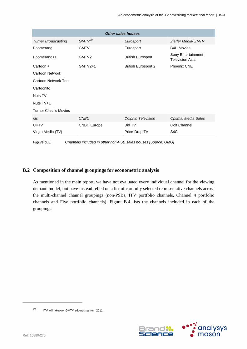
An econometric analysis of the TV advertising market: final report | B–3
Ref: 15880-275
Other sales houses
Turner Broadcasting GMTV30 Eurosport Zierler Media/ ZMTV
Boomerang GMTV Eurosport B4U Movies
Boomerang+1 GMTV2 British Eurosport Sony Entertainment Television Asia
Cartoon + GMTV2+1 British Eurosport 2 Phoenix CNE
Cartoon Network
Cartoon Network Too
Cartoonito
Nuts TV
Nuts TV+1
Turner Classic Movies
ids CNBC Dolphin Television Optimal Media Sales
UKTV CNBC Europe Bid TV Golf Channel
Virgin Media (TV) Price-Drop TV S4C
Figure B.3: Channels included in other non-PSB sales houses [Source: OMG]
B.2 Composition of channel groupings for econometric analysis
As mentioned in the main report, we have not evaluated every individual channel for the viewing demand model, but have instead relied on a list of carefully selected representative channels across the multi-channel channel groupings (non-PSBs, ITV portfolio channels, Channel 4 portfolio channels and Five portfolio channels). Figure B.4 lists the channels included in each of the groupings.
30 ITV will takeover GMTV advertising from 2011.

An econometric analysis of the TV advertising market: final report | B–4
Ref: 15880-275
ITV portfolio channels C4 portfolio channels Five portfolio channels Non-PSBs
CITV E4 Fiver DAVE
ITV2 Film 4 Five USA Discovery channel
ITV3 More 4 Eurosport
ITV4 FX
Men & Motors Living
M4usic
MTV2
Nickolodeon
Sky 1
Sky Movies Premiere
Sky News
Sky Sports 1
TCM
Virgin 1
Yesterday
DAVE
Figure B.4: List of the channels included in the channel groupings for the viewing demand model

An econometric analysis of the TV advertising market: final report | C–1
Ref: 15880-275
Annex C: Further comparison between flexibilities and elasticities
The advertising demand model estimated in this report is an inverse demand system that relates the station average price (CPT) received by the different channel groupings to the quantity of commercial impacts provided by these channels across the period modelled (January 2002 – July 2009). In this inverse demand system, the object of interest is the matrix of own- and cross-price flexibilities of demand.
Following Houck (1965)31
However, inverse demand estimations (and consequently flexibilities) are a common tool only in the agricultural and natural resource economics literature
, flexibilities are defined as “the percentage change in the price of a commodity associated with a 1 percent increase in the quantity demanded of that commodity..., all else remaining constant.” By contrast, the object of interest in a typical direct demand system is the matrix of own- and cross-price elasticities of demand, given by the percentage change in the quantity of a good associated with a 1 percent increase in the price of that good. As a consequence, for a single demand curve, there is an intuitive relationship between the true own-price flexibility and the true own-price elasticity: these are simply the inverse of each other.
32
The purpose of this Annex is to clarify the connection between inverse demand system estimation and “regular” demand system estimation, focusing on the distinction between flexibilities and elasticities and highlighting problems which do not allow for a direct conversion between the two concepts in the context of our study.
but are otherwise rarely used. Several peer reviewers to this study have therefore noted that flexibilities may be an unfamiliar concept to the typical reader. This has consequently led us to introduce the term ‘price inverse elasticity’ which should lead to a more intuitive understanding of the meaning underlying our estimates.
As noted by Huang (2005)33, the relationship between flexibilities and elasticities is complicated by the fact that we can only estimate the underlying parameters. By its very nature, an ordinary least squares (OLS) regression minimises the sum of squared residuals in the dimension of the dependent variable (in this report, prices).34
31 Houck, J., “The relationship of direct price flexibilities to direct price elasticities,” Journal of Farm Economics, 1965, 47 (3), 789–792.
Even for a single demand curve, the Cauchy-Schwarz
32 cf. Park, H. and W. Thurman, “On interpreting Inverse Demand Systems: A primal comparison of scale flexibilities and income elasticities,” American Journal of Agricultural Economics, 1999, 81, 950–958 and the references cited there
33 Huang, K., “How reliable is it to obtain price flexibilities from inverting price elasticities?,” 2005. Working Paper, Economic Research Service, U.S. Department of Agriculture.
34 As described in the body of the report, we argue that OLS yields consistent estimates of the own- and cross-price flexibilities in the advertising market. The same logic would apply, however, if we were using Instrumental Variables estimation to identify the key parameters.

An econometric analysis of the TV advertising market: final report | C–2
Ref: 15880-275
inequality can be used to show that the own-price elasticity, jjε , and the own-price flexibility, jjf ,
are therefore related as follows:
jjjjjjjj f
f ˆ1ˆ1ˆˆ ≥⇒≤ εε
Equation 5: Cauchy-Schwarz inequality describing the relationship between flexibilities and elasticities
It follows from Equation 5 that the estimated own-price flexibilities and elasticities will not necessarily be identical. In contrast, the above equation highlights that it the own-price elasticity will be less elastic than that implied by the inverse of the estimated own-price flexibility.
The comparability between elasticities and flexibilities is further complicated by the fact that our study is based on a demand system. For demand or inverse demand systems, the simple relationship between elasticities and flexibilities no longer holds. If Ω is the matrix of true own-price flexibilities, then Ω-1 is the matrix of true own-price elasticities. In order to derive the set of own-price elasticities Ω -1 corresponding to the own-price flexibility matrix Ω, the (non -diagonal) matrix Ω must be inverted. The values of the own-price elasticities are therefore influenced by the relevant cross-terms.
Another factor adding to the complexity of the situation is that, in an inverse demand system, the own-price flexibility holds constant the quantities of the other products while the own-price elasticity holds constant their prices. This differential conditioning destroys the simple relationship from the one-good case and doesn’t allow general conclusions.
Taking into account these constraints concerning the comparability of elasticities and flexibilities, Figure C.1 and Figure C.2 nonetheless present our system of estimated short-run flexibilities and the corresponding inverse set of short-run (regular) elasticities for the four main channel groupings. While not strictly correct, for the remainder of this annex, we refer to the latter as our “estimates” of the matrix of own- and cross-price elasticities.
ITV1 C4 Five Non PSBs
ITV1 -1.05 - -0.43 -
C4 -0.41 -0.88 - -0.34
Five 0.28 - -0.75 0.32
Non PSBs / Rest of the market
-0.20 -0.18 - -1.10
Figure C.1: Own- and cross-price short-run flexibilities for TV advertising [Analysys Mason,
BrandScience]

An econometric analysis of the TV advertising market: final report | C–3
Ref: 15880-275
ITV1 C4 Five Non PSBs
ITV1 -0.94 - 35 0.49 -35
C4 0.40 -1.29 -35 0.28
Five -0.33 -35 -1.12 -0.36
Non PSBs / Rest of the market 0.13 0.16 -35 -0.97
Figure C.2: Own- and cross-price short-run elasticities for TV advertising [Analysys Mason,
BrandScience]
While the diagonal elements are not the simple inverses, the general pattern between own-product flexibilities and elasticities follows our intuition. Inverse demand for products that are estimated to be flexible (i.e. jjf < −136
jjε) yield inelastic estimates of direct demand (i.e. > −137
Generally increases in prices lead to increases in revenues when demand is elastic (and vice versa). Note that these patterns come through for our scenarios using (as an approximation only) the implied elasticity matrix above. In the case of harmonising down, which implies an increase in price for non-PSBs, applying our estimates yields an estimated less-than-equal reduction in quantity and thus an increase in revenues (as demand for advertising on non-PSBs is “estimated” to be inelastic).
), and vice
versa.
Similarly, in the case of harmonising up, implying a reduction in prices for PSBs, yields an estimated less than-equal reduction in quantity, at least for ITV1, and thus also a reduction in revenue. This reduction is less pronounced for Channel 4 and Five as the demand curves for these channels are “estimated” to be elastic.
The part of the results which has raised concerns about the validity of this transformation process concerns the cross-price elasticities presented in Figure C.2. Several of the values for the cross-price elasticities have changed sign when inverting the flexibility matrix.
We would expect that these counter-intuitive results are mainly driven by a combination of the factors discussed above. This has led us to not present any regular elasticity estimates in the main body of this report. It should also be noted that the use of elasticities could constitute a slightly misleading concept in the context of the advertising market, as it neglects those market mechanisms which have led us to choose an inverse demand framework, i.e. the fact that it is rather the quantity of goods in the market which drives the price rather than the price driving the quantity of goods supplied.
35 Results for those flexibilities which have not been included in Figure C.1 have been deleted from the presentation of the elasticity matrix.
36 To avoid confusion we mean here that the absolute value of the flexibility is greater than 1
37 To avoid confusion we mean here that the value of the elasticity is between 0 and –1

An econometric analysis of the TV advertising market: final report | D–1
Ref: 15880-275
Annex D: Outputs from the econometric analysis
OLS Regression output
Dependent Variable:
Cost per Thousand (ITV1)
Method: Least Squares
Sample (adjusted): 2002M03 2009M07
Included observations: 89 after adjustments
Newey-West HAC Standard Errors & Covariance (lag truncation=3)
Coefficient Std. Error t-Statistic Prob.
Constant 26.143 12.036 2.172 0.033
June 2006 -0.452 0.179 -2.522 0.014
July 2006 -1.261 0.259 -4.866 0.000
January 0.849 0.257 3.307 0.001
June -0.504 0.198 -2.551 0.013
August -1.033 0.143 -7.222 0.000
October 0.794 0.249 3.188 0.002
November 1.135 0.166 6.843 0.000
LN (Internet impacts)
-0.494 0.570 -0.866 0.389
FTSE index 0.000 0.000 3.502 0.001
LN (SOC – ITV1) 3.488 2.076 1.681 0.097
Impacts (ITV1) -0.000000244 0.000 -6.583 0.000
Impacts (C4) -0.000000226 0.000 -3.596 0.001
Impacts (Five) 0.000000234 0.000 2.148 0.035
Impacts (Rest of market)
-0.000000062 0.000 -1.852 0.068
Lagged prices (t-1) 0.319 0.138 2.303 0.024
Lagged prices (t-2) -0.294 0.106 -2.777 0.007
R-squared 0.87 Mean dependent var 5.35
Adjusted R-squared
0.85 S.D. dependent var 1.06
S.E. of regression 0.42 Akaike info criterion 1.25
Sum squared resid 12.43 Schwarz criterion 1.73
Log likelihood -38.70 Hannan-Quinn criter. 1.44
F-statistic 31.25 Durbin-Watson stat 1.89
Prob(F-statistic) 0.00 Hannan-Quinn criter.
Figure D.1: OLS output for secondary ITV1 regression [Source: Analysys Mason, BrandScience]

An econometric analysis of the TV advertising market: final report | D–2
Ref: 15880-275
OLS Regression output
Dependent Variable:
Cost per Thousand (ITV1)
Method: Least Squares
Sample (adjusted): 2002M03 2009M07
Included observations: 89 after adjustments
Newey-West HAC Standard Errors & Covariance (lag truncation=3)
Coefficient Std. Error t-Statistic Prob.
Constant 31.786 10.404 3.055 0.003
June 2006 -0.404 0.201 -2.012 0.048
July 2006 -1.239 0.275 -4.498 0.000
January 0.791 0.252 3.142 0.002
June -0.528 0.203 -2.598 0.011
August -1.027 0.165 -6.223 0.000
October 0.823 0.243 3.387 0.001
November 1.173 0.171 6.844 0.000
LN (Internet impacts) -0.829 0.481 -1.723 0.089
FTSE index 0.000 0.000 2.919 0.005
LN (SOCI – ITV family) 1.595 2.523 0.632 0.529
Impacts (ITV family) -0.000000238 0.000 -5.313 0.000
Impacts (C4) -0.000000260 0.000 -3.697 0.000
Impacts (Five) 0.000000262 0.000 2.105 0.039
Impacts (Rest of market) -0.000000006 0.000 -0.135 0.893
Lagged prices (t-1) 0.359 0.137 2.623 0.011
Lagged prices (t-2) -0.256 0.103 -2.484 0.015
R-squared 0.86 Mean dependent var 5.35
Adjusted R-squared 0.83 S.D. dependent var 1.06
S.E. of regression 0.44 Akaike info criterion 1.36
Sum squared resid 13.81 Schwarz criterion 1.83
Log likelihood -43.36 Hannan-Quinn criter. 1.55
F-statistic 27.69 Durbin-Watson stat 1.85
Prob(F-statistic) 0.00
Figure D.2: OLS output for secondary ITV1 regression [Source: Analysys Mason, BrandScience]

An econometric analysis of the TV advertising market: final report | D–3
Ref: 15880-275
OLS Regression output
Dependent Variable:
Cost per Thousand (ITV family)
Method: Least Squares
Sample (adjusted): 2002M03 2009M07
Included observations: 89 after adjustments
Newey-West HAC Standard Errors & Covariance (lag truncation=3)
Coefficient Std. Error t-Statistic Prob.
Constant 24.147 11.283 2.140 0.036
June 2006 -0.523 0.168 -3.105 0.003
July 2006 -1.273 0.241 -5.283 0.000
January 0.872 0.257 3.390 0.001
June -0.511 0.190 -2.683 0.009
August -0.971 0.134 -7.230 0.000
October 0.707 0.246 2.873 0.005
November 1.028 0.163 6.319 0.000
LN (Internet impacts) -0.446 0.537 -0.830 0.409
FTSE index 0.000 0.000 3.374 0.001
LN (SOCI – ITV1) 3.174 1.948 1.629 0.108
Impacts (ITV1) -0.000000217 0.000 -6.139 0.000
Impacts (C4) -0.000000193 0.000 -3.210 0.002
Impacts (Five) 0.000000171 0.000 1.597 0.115
Impacts (Rest of market) -0.000000073 0.000 -2.366 0.021
Lagged prices (t-1) 0.364 0.144 2.531 0.014
Lagged prices (t-2) -0.323 0.111 -2.905 0.005
R-squared 0.88 Mean dependent var
Adjusted R-squared 0.86 S.D. dependent var
S.E. of regression 0.40 Akaike info criterion
Sum squared resid 11.34 Schwarz criterion
Log likelihood -34.59 Hannan-Quinn criter.
F-statistic 33.79 Durbin-Watson stat
Prob(F-statistic) 0.00
Figure D.3: OLS output for main ITV family regression [Source: Analysys Mason, BrandScience]

An econometric analysis of the TV advertising market: final report | D–4
Ref: 15880-275
OLS Regression output
Dependent Variable:
Cost per Thousand (ITV family)
Method: Least Squares
Sample (adjusted): 2002M03 2009M07
Included observations: 89 after adjustments
Newey-West HAC Standard Errors & Covariance (lag truncation=3)
Coefficient Std. Error t-Statistic Prob.
Constant 28.672 9.755 2.939 0.004
June 2006 -0.451 0.182 -2.477 0.016
July 2006 -1.261 0.254 -4.962 0.000
January 0.825 0.252 3.280 0.002
June -0.522 0.191 -2.739 0.008
August -0.970 0.153 -6.325 0.000
October 0.743 0.232 3.209 0.002
November 1.082 0.160 6.768 0.000
LN (Internet impacts) -0.699 0.456 -1.534 0.129
FTSE index 0.000 0.000 3.075 0.003
LN (SOCI – ITV family) 2.231 2.479 0.900 0.371
Impacts (ITV family) -0.000000218 0.000 -5.210 0.000
Impacts (C4) -0.000000224 0.000 -3.364 0.001
Impacts (Five) 0.000000218 0.000 1.828 0.072
Impacts (Rest of market) -0.000000019 0.000 -0.465 0.643
Lagged prices (t-1) 0.386 0.142 2.710 0.008
Lagged prices (t-2) -0.290 0.111 -2.626 0.011
R-squared 0.87 Mean dependent var 5.05
Adjusted R-squared 0.85 S.D. dependent var 1.05
S.E. of regression 0.41 Akaike info criterion 1.23
Sum squared resid 12.12 Schwarz criterion 1.70
Log likelihood -37.55 Hannan-Quinn criter. 1.42
F-statistic 31.33 Durbin-Watson stat 1.86
Prob(F-statistic) 0.00
Figure D.4: OLS output for secondary ITV family regression [Source: Analysys Mason, BrandScience]

An econometric analysis of the TV advertising market: final report | D–5
Ref: 15880-275
OLS Regression output
Dependent Variable:
Cost per Thousand (C4)
Method: Least Squares
Sample (adjusted): 2002M03 2009M07
Included observations: 89 after adjustments
Newey-West HAC Standard Errors & Covariance (lag truncation=3)
Coefficient Std. Error t-Statistic Prob.
Constant 39.829 8.437 4.721 0.000
June 2006 -1.023 0.169 -6.043 0.000
July 2006 -0.853 0.139 -6.152 0.000
January 0.484 0.225 2.151 0.035
March 0.410 0.155 2.654 0.010
May 0.522 0.132 3.961 0.000
June -0.615 0.208 -2.951 0.004
July -0.419 0.179 -2.337 0.023
August -1.011 0.176 -5.731 0.000
September 1.158 0.230 5.040 0.000
October 1.027 0.262 3.913 0.000
November 1.618 0.168 9.656 0.000
Year 2002 -1.272 0.309 -4.118 0.000
Year 2003 -0.979 0.238 -4.112 0.000
Year 2004 -0.320 0.186 -1.719 0.090
LN (Internet impacts) -0.949 0.332 -2.860 0.006
FTSE index 0.000 0.000 3.401 0.001
LN (SOCI – C4) 2.650 2.020 1.312 0.194
Impacts (ITV1) -0.000000060 0.000 -1.327 0.189
Impacts (C4) -0.000000502 0.000 -8.491 0.000
Impacts (Five) -0.000000063 0.000 -0.499 0.620
Impacts (Rest of market) -0.000000058 0.000 -1.776 0.080
Lagged prices (t-1) 0.176 0.094 1.868 0.066
Lagged prices (t-2) -0.196 0.090 -2.172 0.033
R-squared 0.94 Mean dependent var 5.64
Adjusted R-squared 0.92 S.D. dependent var 1.20
S.E. of regression 0.33 Akaike info criterion 0.86
Sum squared resid 7.15 Schwarz criterion 1.53
Log likelihood -14.09 Hannan-Quinn criter. 1.13
F-statistic 47.25 Durbin-Watson stat 1.90
Prob(F-statistic) 0.00
Figure D.5: OLS output for main C4 regression [Source: Analysys Mason, BrandScience]

An econometric analysis of the TV advertising market: final report | D–6
Ref: 15880-275
OLS Regression output
Dependent Variable:
Cost per Thousand (C4)
Method: Least Squares
Sample (adjusted): 2003M01 2009M07
Included observations: 79 after adjustments
Newey-West HAC Standard Errors & Covariance (lag truncation=3)
Coefficient Std. Error t-Statistic Prob.
Constant 40.020 9.478 4.222 0.000
June 2006 -0.781 0.178 -4.388 0.000
July 2006 -0.834 0.160 -5.206 0.000
January 0.632 0.209 3.032 0.004
March 0.467 0.156 3.000 0.004
May 0.595 0.161 3.691 0.001
June -0.641 0.249 -2.578 0.013
July -0.316 0.203 -1.558 0.125
August -0.997 0.176 -5.656 0.000
September 1.267 0.254 4.980 0.000
October 0.917 0.288 3.180 0.002
November 1.777 0.153 11.647 0.000
Year 2002 0.000 0.000 0.000 0.000
Year 2003 -0.817 0.227 -3.592 0.001
Year 2004 -0.420 0.171 -2.455 0.017
LN (Internet impacts) -0.983 0.352 -2.791 0.007
FTSE index 0.000 0.000 3.875 0.000
LN (SOCI – C4 family) 2.645 1.272 2.079 0.042
Impacts (ITV1) -0.000000115 0.000 -2.763 0.008
Impacts (C4 family) -0.000000362 0.000 -6.792 0.000
Impacts (Five) -0.000000089 0.000 -0.734 0.466
Impacts (Rest of market) -0.000000027 0.000 -0.911 0.366
Lagged prices (t-1) 0.242 0.104 2.337 0.023
Lagged prices (t-2) -0.245 0.081 -3.026 0.004
R-squared 0.94 Mean dependent var 5.56
Adjusted R-squared 0.92 S.D. dependent var 1.17
S.E. of regression 0.33 Akaike info criterion 0.89
Sum squared resid 6.28 Schwarz criterion 1.58
Log likelihood -12.09 Hannan-Quinn criter. 1.16
F-statistic 40.81 Durbin-Watson stat 1.93
Prob(F-statistic) 0.00
Figure D.6: OLS output for secondary C4 regression [Source: Analysys Mason, BrandScience]

An econometric analysis of the TV advertising market: final report | D–7
Ref: 15880-275
OLS Regression output
Dependent Variable:
Cost per Thousand (C4 family)
Method: Least Squares
Sample (adjusted): 2003M01 2009M07
Included observations: 79 after adjustments
Newey-West HAC Standard Errors & Covariance (lag truncation=3)
Coefficient Std. Error t-Statistic Prob.
Constant 42.860 12.853 3.335 0.002
June 2006 -0.612 0.260 -2.355 0.022
July 2006 -0.831 0.182 -4.571 0.000
January 0.623 0.266 2.346 0.023
March 0.427 0.188 2.270 0.027
May 0.328 0.173 1.895 0.063
June -1.076 0.274 -3.920 0.000
July -0.592 0.216 -2.746 0.008
August -1.113 0.236 -4.710 0.000
September 0.977 0.321 3.047 0.004
October 0.662 0.284 2.327 0.024
November 1.535 0.233 6.583 0.000
Year 2003 -0.867 0.363 -2.386 0.020
Year 2004 -0.234 0.264 -0.887 0.379
LN (Internet impacts) -1.162 0.513 -2.263 0.028
FTSE index 0.000 0.000 1.932 0.058
LN (SOCI – C4) 1.704 2.256 0.755 0.453
Impacts (ITV1) -0.000000078 0.000 -1.489 0.142
Impacts (C4) -0.000000497 0.000 -5.349 0.000
Impacts (Five) 0.000000021 0.000 0.128 0.898
Impacts (Rest of market) -0.000000069 0.000 -1.943 0.057
Lagged prices (t-1) 0.282 0.115 2.443 0.018
Lagged prices (t-2) -0.221 0.118 -1.870 0.067
R-squared 0.93 Mean dependent var 5.22
Adjusted R-squared 0.91 S.D. dependent var 1.23
S.E. of regression 0.38 Akaike info criterion 1.13
Sum squared resid 7.97 Schwarz criterion 1.82
Log likelihood -21.51 Hannan-Quinn criter. 1.40
F-statistic 34.98 Durbin-Watson stat 1.85
Prob(F-statistic) 0.00
Figure D.7: OLS output for main C4 family regression [Source: Analysys Mason, BrandScience]

An econometric analysis of the TV advertising market: final report | D–8
Ref: 15880-275
OLS Regression output
Dependent Variable:
Cost per Thousand (C4 family)
Method: Least Squares
Sample (adjusted): 2003M01 2009M07
Included observations: 79 after adjustments
Newey-West HAC Standard Errors & Covariance (lag truncation=3)
Coefficient Std. Error t-Statistic Prob.
Constant 45.205 9.451 4.783 0.000
June 2006 -0.326 0.202 -1.611 0.113
July 2006 -0.746 0.176 -4.247 0.000
January 0.756 0.204 3.697 0.000
March 0.471 0.168 2.812 0.007
May 0.403 0.155 2.608 0.012
June -0.919 0.254 -3.621 0.001
July -0.472 0.198 -2.381 0.021
August -1.086 0.199 -5.464 0.000
September 1.004 0.280 3.585 0.001
October 0.735 0.276 2.660 0.010
November 1.660 0.173 9.573 0.000
Year 2003 -0.772 0.227 -3.397 0.001
Year 2004 -0.356 0.178 -2.007 0.050
LN (Internet impacts) -1.123 0.359 -3.126 0.003
FTSE index 0.000 0.000 3.259 0.002
LN (SOCI – C4 family) 3.742 1.302 2.873 0.006
Impacts (ITV1) -0.000000131 0.000 -3.243 0.002
Impacts (C4 – C4 family) -0.000000410 0.000 -6.868 0.000
Impacts (Five) 0.000000036 0.000 0.293 0.771
Impacts (Rest of market) -0.000000029 0.000 -0.918 0.363
Lagged prices (t-1) 0.274 0.113 2.420 0.019
Lagged prices (t-2) -0.229 0.095 -2.406 0.019
R-squared 0.95 Mean dependent var 5.22
Adjusted R-squared 0.93 S.D. dependent var 1.23
S.E. of regression 0.33 Akaike info criterion 0.85
Sum squared resid 6.03 Schwarz criterion 1.54
Log likelihood -10.50 Hannan-Quinn criter. 1.12
F-statistic 47.05 Durbin-Watson stat 2.02
Prob(F-statistic) 0.00
Figure D.8: OLS output for secondary C4 family regression [Source: Analysys Mason, BrandScience]

An econometric analysis of the TV advertising market: final report | D–9
Ref: 15880-275
OLS Regression output
Dependent Variable:
Cost per Thousand (Five)
Method: Least Squares
Sample (adjusted): 2002M03 2009M07
Included observations: 89 after adjustments
Newey-West HAC Standard Errors & Covariance (lag truncation=3)
Coefficient Std. Error t-Statistic Prob.
Constant 11.714 5.233 2.239 0.028
June 2006 -0.744 0.107 -6.971 0.000
July 2006 -0.429 0.144 -2.969 0.004
February -0.234 0.096 -2.423 0.018
June -0.520 0.116 -4.466 0.000
July -0.420 0.100 -4.187 0.000
August -0.655 0.125 -5.249 0.000
September 0.578 0.158 3.663 0.000
October 0.621 0.195 3.175 0.002
November 0.896 0.182 4.929 0.000
December -0.291 0.225 -1.294 0.200
Year 2009 -0.730 0.152 -4.814 0.000
LN (Internet impacts) -0.011 0.224 -0.048 0.962
FTSE index 0.000 0.000 2.831 0.006
LN (SOCI - Five) 2.061 0.788 2.614 0.011
Impacts (ITV1) -0.000000063 0.000 -3.296 0.002
Impacts (C4) -0.000000017 0.000 -0.520 0.605
Impacts (Five) -0.000000397 0.000 -3.784 0.000
Impacts (Rest of market) -0.000000016 0.000 -0.799 0.427
Lagged prices (t-1) 0.236 0.122 1.939 0.057
Lagged prices (t-2) -0.169 0.053 -3.159 0.002
R-squared 0.92 Mean dependent var 3.45
Adjusted R-squared 0.90 S.D. dependent var 0.68
S.E. of regression 0.22 Akaike info criterion -0.02
Sum squared resid 3.20 Schwarz criterion 0.57
Log likelihood 21.76 Hannan-Quinn criter. 0.22
F-statistic 39.61 Durbin-Watson stat 1.81
Prob(F-statistic) 0.00
Figure D.9: OLS output for main Five regression [Source: Analysys Mason, BrandScience]

An econometric analysis of the TV advertising market: final report | D–10
Ref: 15880-275
OLS Regression output
Dependent Variable:
Cost per Thousand (Five)
Method: Least Squares
Sample (adjusted): 2002M03 2009M07
Included observations: 89 after adjustments
Newey-West HAC Standard Errors & Covariance (lag truncation=3)
Coefficient Std. Error t-Statistic Prob.
Constant -2.320 5.506 -0.421 0.675
June 2006 -0.770 0.124 -6.232 0.000
July 2006 -0.427 0.143 -2.996 0.004
February -0.205 0.098 -2.093 0.040
June -0.504 0.116 -4.358 0.000
July -0.382 0.089 -4.281 0.000
August -0.639 0.111 -5.757 0.000
September 0.557 0.165 3.370 0.001
October 0.577 0.174 3.317 0.001
November 0.864 0.155 5.558 0.000
December -0.241 0.192 -1.256 0.214
Year 2009 -0.719 0.143 -5.027 0.000
LN (Internet impacts) 0.348 0.247 1.408 0.164
FTSE index 0.000 0.000 2.577 0.012
LN (SOCI – Five family) -0.411 0.834 -0.493 0.623
Impacts (ITV1) -0.000000048 0.000 -2.769 0.007
Impacts (C4) -0.000000037 0.000 -1.147 0.255
Impacts (Five family) -0.000000403 0.000 -4.171 0.000
Impacts (Rest of market) -0.000000027 0.000 -1.433 0.156
Lagged prices (t-1) 0.239 0.110 2.164 0.034
Lagged prices (t-2) -0.152 0.050 -3.032 0.003
R-squared 0.92 Mean dependent var 3.45
Adjusted R-squared 0.90 S.D. dependent var 0.68
S.E. of regression 0.22 Akaike info criterion -0.03
Sum squared resid 3.17 Schwarz criterion 0.56
Log likelihood 22.18 Hannan-Quinn criter. 0.21
F-statistic 40.01 Durbin-Watson stat 1.82
Prob(F-statistic) 0.00
Figure D.10: OLS output for secondary Five regression [Source: Analysys Mason, BrandScience]

An econometric analysis of the TV advertising market: final report | D–11
Ref: 15880-275
OLS Regression output
Dependent Variable:
Cost per Thousand (Five family)
Method: Least Squares
Sample (adjusted): 2002M03 2009M07
Included observations: 89 after adjustments
Newey-West HAC Standard Errors & Covariance (lag truncation=3)
Coefficient Std. Error t-Statistic Prob.
Constant 17.832 4.753 3.752 0.000
June 2006 -0.677 0.118 -5.721 0.000
July 2006 -0.335 0.143 -2.343 0.022
February -0.201 0.089 -2.252 0.028
June -0.510 0.124 -4.120 0.000
July -0.411 0.116 -3.532 0.001
August -0.595 0.130 -4.568 0.000
September 0.634 0.149 4.239 0.000
October 0.545 0.181 3.013 0.004
November 0.745 0.154 4.823 0.000
December -0.422 0.207 -2.040 0.045
Year 2009 -0.569 0.136 -4.182 0.000
LN (Internet impacts) -0.283 0.206 -1.375 0.174
FTSE index 0.000 0.000 2.747 0.008
LN (SOCI - Five) 2.387 0.642 3.716 0.000
Impacts (ITV1) -0.000000072 0.000 -3.393 0.001
Impacts (C4) -0.000000001 0.000 -0.024 0.981
Impacts (Five) -0.000000263 0.000 -3.182 0.002
Impacts (Rest of market) -0.000000006 0.000 -0.325 0.746
Lagged prices (t-1) 0.321 0.126 2.554 0.013
Lagged prices (t-2) -0.179 0.061 -2.961 0.004
R-squared 0.93 Mean dependent var 3.34
Adjusted R-squared 0.91 S.D. dependent var 0.68
S.E. of regression 0.21 Akaike info criterion -0.12
Sum squared resid 2.89 Schwarz criterion 0.47
Log likelihood 26.24 Hannan-Quinn criter. 0.12
F-statistic 44.79 Durbin-Watson stat 1.96
Prob(F-statistic) 0.00
Figure D.11: OLS output for main Five family regression [Source: Analysys Mason, BrandScience]

An econometric analysis of the TV advertising market: final report | D–12
Ref: 15880-275
OLS Regression output
Dependent Variable:
Cost per Thousand (Five family)
Method: Least Squares
Sample (adjusted): 2002M03 2009M07
Included observations: 89 after adjustments
Newey-West HAC Standard Errors & Covariance (lag truncation=3)
Coefficient Std. Error t-Statistic Prob.
Constant 7.604 5.138 1.480 0.143
June 2006 -0.775 0.127 -6.103 0.000
July 2006 -0.357 0.145 -2.461 0.016
February -0.179 0.099 -1.820 0.073
June -0.537 0.117 -4.603 0.000
July -0.411 0.095 -4.349 0.000
August -0.594 0.121 -4.918 0.000
September 0.606 0.154 3.929 0.000
October 0.552 0.172 3.201 0.002
November 0.744 0.154 4.827 0.000
December -0.324 0.194 -1.670 0.099
Year 2009 -0.474 0.134 -3.549 0.001
LN (Internet impacts) 0.045 0.241 0.184 0.854
FTSE index 0.000 0.000 3.921 0.000
LN (SOCI – Five family) 1.220 0.676 1.805 0.076
Impacts (ITV1) -0.000000051 0.000 -2.707 0.009
Impacts (C4) -0.000000001 0.000 -0.032 0.974
Impacts (Five family) -0.000000366 0.000 -4.028 0.000
Impacts (Rest of market) -0.000000029 0.000 -1.499 0.138
Lagged prices (t-1) 0.311 0.120 2.591 0.012
Lagged prices (t-2) -0.155 0.060 -2.592 0.012
R-squared 0.93 Mean dependent var 3.34
Adjusted R-squared 0.91 S.D. dependent var 0.68
S.E. of regression 0.20 Akaike info criterion -0.14
Sum squared resid 2.84 Schwarz criterion 0.45
Log likelihood 27.07 Hannan-Quinn criter. 0.10
F-statistic 45.69 Durbin-Watson stat 1.88
Prob(F-statistic) 0.00
Figure D.12: OLS output for secondary Five family regression [Source: Analysys Mason,
BrandScience]

An econometric analysis of the TV advertising market: final report | D–13
Ref: 15880-275
OLS Regression output
Dependent Variable:
Cost per Thousand (Non PSBs)
Method: Least Squares
Sample (adjusted): 2002M02 2009M07
Included observations: 90 after adjustments
Newey-West HAC Standard Errors & Covariance (lag truncation=3)
Coefficient Std. Error t-Statistic Prob.
Constant 5.408 6.190 0.874 0.385
June 2006 -0.401 0.080 -4.992 0.000
July 2006 -0.475 0.076 -6.267 0.000
January 0.913 0.188 4.861 0.000
February 0.449 0.111 4.063 0.000
March 0.647 0.074 8.697 0.000
April 0.488 0.069 7.095 0.000
May 0.582 0.063 9.171 0.000
September 1.121 0.130 8.644 0.000
October 0.527 0.084 6.248 0.000
November 0.765 0.085 9.044 0.000
LN (Internet impacts) 0.071 0.218 0.327 0.745
FTSE index 0.000 0.000 0.304 0.762
LN (SOCI – Non PSBs) 2.156 0.722 2.985 0.004
Impacts (ITV1) -0.000000021 0.000 -1.099 0.276
Impacts (C4) -0.000000102 0.000 -2.573 0.012
Impacts (Five) 0.000000147 0.000 2.250 0.028
Impacts (Non PSBs) -0.000000187 0.000 -7.433 0.000
Lagged prices (t-1) 0.608 0.116 5.237 0.000
R-squared 0.95 Mean dependent var 3.16
Adjusted R-squared 0.94 S.D. dependent var 0.74
S.E. of regression 0.18 Akaike info criterion -0.37
Sum squared resid 2.40 Schwarz criterion 0.16
Log likelihood 35.43 Hannan-Quinn criter. -0.15
F-statistic 75.23 Durbin-Watson stat 2.10
Prob(F-statistic) 0.00
Figure D.13: OLS output for secondary Five family regression [Source: Analysys Mason,
BrandScience]
An econometric analysis of the TV advertising market: final report | E–1
Ref: 15880-275
Annex E: Analysis of policy options
Our econometric analysis has provided a quantitative tool to understand the mechanics of the UK TV advertising market, and to estimate channels’ reactions to a change in the regulatory environment. Based on our modelling, we have developed a set of scenarios which are intended to inform Ofcom on the potential effects that changes to the COSTA rules could have on the advertising revenues of the defined channel groupings. (Note that these scenarios have not been endorsed by Ofcom and do not necessarily reflect Ofcom’s views on potential policy options.) In order to develop this comparative analysis, this section commences by introducing the methodology behind the policy evaluation, discusses key assumptions underlying our analysis with regard to the future supply of commercial impacts, and then presents the results of our analysis.
E.1 Methodology used for the analysis of policy options
The aim of our econometric model is to describe how changes in the COSTA rules affect advertising revenue streams. We have built a model which is aimed at specifically explaining causal relations in the two markets we have considered. This allows us to derive the demand for TV advertising, but does not enable us to draw conclusions on the utility derived by consumers from watching TV, nor the cost structure of the industry, both of which would be required to conduct a total welfare analysis. Such an analysis is outside the scope of our present study.
As described in the main report, our analysis applies a two-stage model that includes an advertising demand model and a viewer demand model to reflect the nature of the TV advertising market. Here we describe how the two models are combined to forecast the net effect on the revenue streams of channels selling TV advertising in the UK. Under our assumption of a perfectly inelastic supply curve, consider a single broadcaster j. A change in the advertising minutes allowed under COSTA rules, leaving aside any reaction of viewers to the increase in the implicit ‘price’ of viewing, can be represented as an outward shift of the supply curve from Sj to Sj′ . Figure E.1 illustrates this effect.

An econometric analysis of the TV advertising market: final report | E–2
Ref: 15880-275
A
B C
S S’
Quantity of impacts
Pric
e of
impa
cts
qj qj’’
pj
pj’’
D
A
B C
S S’
Quantity of impacts
Pric
e of
impa
cts
qj qj’’
pj
pj’’
D
Figure E.1: Effect of an increase in the amount of commercial minutes (no viewing impact)
By holding viewing figures constant, an increase in the advertising minutage directly increases the quantity of commercial impacts qj supplied by channel grouping j. In our example, the quantity supplied shifts from qj to qj′. The increase in the supply of commercial impacts triggers a fall in price, and a subsequent rise in the demand for impacts from advertisers, until an equilibrium is reached and demand again matches supply.
We use our estimates of the price inverse elasticities as calculated from our advertiser demand model (Equation 1 on page 31) to calculate the revenue effect of a change in COSTA rules. In Figure E.1, prices change from pj to pj′. This allows us to directly derive the revenue effects for broadcaster j. Prior to the change in COSTA rules, revenue from advertising equalled A + B. Following the change in COSTA rules allowing for an increase in the amount of advertising airtime, revenue equals B + C. Whether this effect constitutes a net gain or a net loss depends critically on the price inverse elasticity of advertisers for commercial impacts from broadcaster j.
The two-sided nature of the advertising market introduces further complexity into this scenario. As outlined in Section 4.2, we model the way in which viewing demand depends on the number of advertising minutes broadcast. It is very likely that viewing will not remain constant following a change in the COSTA rules: viewers consider advertising breaks an implicit price for access to particular content, and will adjust their viewing accordingly based on their preferences for content and the price they have to pay. Our viewing demand model provides estimates of the reaction of viewers to an increase in advertising by broadcaster j. Users are likely to reduce their amount of viewing if broadcaster j increases the advertising minutes on its programming, as was shown in the results in Section 5.2. Figure E.2(below) incorporates this negative effect on the supply of

An econometric analysis of the TV advertising market: final report | E–3
Ref: 15880-275
commercial impacts, stemming from reduced viewing, which results from an increase in the number of advertising minutes.
B C1
S S’
Quantity of impacts
Pric
e of
impa
cts
qj qj’’
pj
pj’’
S’’
C2
C3
A1
A2
qj’’’
pj’’’
DB C1
S S’
Quantity of impacts
Pric
e of
impa
cts
qj qj’’
pj
pj’’
S’’
C2
C3
A1
A2
qj’’’
pj’’’
D
Figure E.2: Effect of an increase in the amount of commercial minutes (full viewing impact)
As before, we assume that an increase in the number of commercial minutes shifts the supply curve to the right. Initially this increase in minutage leads to an increase in the quantity of commercial impacts supplied: qj to qj′. Following the increase in the ‘price’ paid by viewers due to a greater number of commercials, the programme audience will decline and the number of impacts decrease. Depending on the viewing demand elasticity, the number of commercial impacts qj could then reduce from qj′ to qj′′. The overall effect is therefore a change in the number of commercial impacts supplied from qj to qj′′. This effect will be smaller than the simple effect considered in Figure E.1.
To illustrate our approach, we consider the following numerical example. Let us assume that we initially hold viewing constant. An increase in the number of minutes of commercials will therefore directly increase the quantity of impacts. For example, if we start with 8 minutes delivering 800 000 commercial impacts, an increase in the number of allowed minutes to 10, the number of commercial impacts increases to 1 000 000. This increase in the quantity of impacts is equivalent to a shift of qj to qj′ in Figure E.1. However, we are unlikely to observe the shift from qj to qj′ as we expect the extra 2 minutes of advertising to negatively impact viewing figures. If the increase in commercial minutage causes the audience to shrink by 10%, the actual quantity of impacts supplied is 910 000 (as represented by qj′′ in Figure E.2).

An econometric analysis of the TV advertising market: final report | E–4
Ref: 15880-275
This combined effect slightly complicates our revenue analysis. The broadcaster initially has advertising revenue equal to B + A1 + A2. Taking into account the dynamics of both the advertising and the viewing market, the combined revenue effect is a change to B + A2 + C1 + C3 compared to a change to B + C1 + C2 in the absence of viewing effects (as shown in Figure E.1). The difference in revenue clearly depends on the outputs of both our models, the advertisers’ price inverse elasticity and the viewers’ advertising elasticity of demand.
This example further illustrates the necessity to address both sides of the advertising market. We are confident that our approach appropriately addresses the idiosyncrasies of the respective markets, and has delivered unbiased estimates of the respective inverse elasticities and regular elasticities which allow for an appropriate assessment of potential changes to the COSTA rules as envisioned by Ofcom.
The scope of our study is to consider the direct impact of changes in the COSTA rules on the advertising market. To that end, we have developed our two demand models described in Section 4. However, a change in regulation for the TV advertising market can also have repercussions going beyond those markets modelled in our policy analysis:
• Significant changes in the revenue levels of broadcasters might trigger pricing reactions in other markets along the TV value chain to balance the change in revenue levels (be it positive or negative). For example, a channel might consider reducing its carriage fees in the case of higher advertising revenues to reach a wider audience, thereby strengthening its own position in the market for commercial impacts. Another potential strategic consideration could concern a revision of investment in programme quality. However, our understanding of the advertising market does not suggest that there are areas which are obvious prime targets for such a strategic move. As a result, it would be difficult to conduct a meaningful analysis at this stage, and we have not considered this aspect any further in our analysis.
• The policy might also affect areas outside the TV value chain. First, there might be substitution effects with other media, in particular with print and internet advertising. Second, changes in the amount of advertisement shown on TV might impact other industries. For example, if less advertising is shown, this is likely to benefit companies holding a large share in their respective market. These larger players will be able to continue to dedicate a significant part of their budget for advertising in a scarcer (i.e. more expensive) market. This will allow them to continue raising awareness for their brands. As a result, changing the COSTA rules may impact the competitiveness in various secondary markets. While such an analysis is beyond the scope of this study.
In addition, this study is not intended to consider changes in surplus for advertisers or viewers. In particular a reduction in advertising minutes may increase the surplus of viewers, even if the elasticity of viewers’ demand for programming has been shown to be small. Similarly an increase in advertising minutes is likely to increase surplus for advertisers. To consider these effects in full it would also be necessary to look in detail at other advertising markets, such as print and the Internet, which is beyond the scope of this study.

An econometric analysis of the TV advertising market: final report | E–5
Ref: 15880-275
E.2 Market developments and the supply of commercial impacts
The advertising industry in general – and the TV advertising market in particular – are currently undergoing a significant amount of change. It is important that our model takes into account the most relevant market developments to arrive at an appropriate estimate of the overall change in revenue streams. We have defined the relevant time frame for our policy analysis to be three years. We feel that this provides an appropriate time frame to take into account long-run effects such as the change in SOCI and provide a meaningful analysis of the implications of a change in the regulatory framework. It is nonetheless straightforward to extend this analysis over a longer period within the scenario planner Excel tool which will be supplied to Ofcom.
Looking at the role of TV advertising in the entire advertising market, the advent of the Internet as a widespread and versatile platform for targeted marketing has recently threatened the dominant position of TV within the industry. The effect of this threat might be a reduction in the willingness to pay for TV advertising, and we have accounted for this by introducing a corresponding variable into our equations.
A key parameter underlying our policy analysis is the forecast of commercial impacts in future periods. Several important market developments have influenced the supply of commercial impacts over recent years, and these have played a key role in determining our forecasts:
• Multi-channel penetration: With cable and satellite platforms penetrating larger parts of the population, the number of channels available in each household has increased significantly. This uptake in multi-channel penetration has led to more dispersed viewing, with viewers substituting away from the flagship channels (as seen in Figure 3.5). It may also have contributed to some growth in the total number of commercial impacts. The digital switchover will reinforce this trend over the following years, as it will make available a much larger number of channels to the majority of households still relying on DTT.
• Secondary and tertiary viewing: The number of TV sets in households has significantly increased over recent years, and many families now have several TVs. This has a direct positive effect on the supply of commercial impacts. Again, this trend is expected to continue over the coming years.
• Change in the composition of households: The number of single households in the UK has grown steadily over the last few years. This has led to more people watching TV on their own and has thereby positively influenced the supply of commercial impacts.
• Non-linear TV viewing: The BBC iPlayer has been immensely successful, and many other channels are following suit. We can therefore expect on-demand viewing to play an increasingly important role over the coming years. Given that there are currently no advertising breaks in such content, the number of commercial impacts supplied by the industry may decrease following the take-up of these services.

An econometric analysis of the TV advertising market: final report | E–6
Ref: 15880-275
• Increased use of PVRs: Personal video recorders allow users to easily store a large number of shows in a significantly more convenient format than VHS did previously, and these devices have been widely taken up by consumers over recent years. In addition, TV platforms such as Sky offer more sophisticated set-top boxes which include PVR functionality and are better integrated into the programming schedule, allowing for even easier recording of shows. As a result, viewers can skip past advertising breaks relatively easily. This could have a significant negative impact on the supply of commercial impacts in the long run, although research to date has shown that this effect is more or less cancelled out by an opposite effect whereby viewers with PVRs tend to watch more TV shows.
Given that these developments could influence the supply of commercial impacts both positively and negatively, we have developed three cases for the supply of future commercial impacts to reflect this uncertainty:
• Strong growth: In this case, the growth in single households, secondary viewing and the increased attractiveness of the wider channel portfolio lead to a strong increase in commercial impacts. At the same time, the growth in multi-channel penetration leads to a more fragmented market, with the SOCI for the flagship channels decreasing over time.
• Intermediate growth: This case reflects the view that the take-up of VoD and PVRs will undermine some of the growth assumed in the strong growth case. At the same time, it is assumed that the flagship channels will be able to prevent some of the substitution towards the smaller channels.
• Flat market: This case assumes zero growth over the coming years, with market shares between channels staying at their 2009 levels. While this appears to be an unlikely case given all the market influences mentioned above, this scenario has the advantage of allowing an evaluation of the “untainted” policy effects, as the results are not affected by changes in the market environment.
Figure E.3 illustrates how the three cases impact the total supply of commercial impacts in the UK TV advertising market.

An econometric analysis of the TV advertising market: final report | E–7
Ref: 15880-275
50
55
60
65
70
75
80
85
90
Oct-06 Apr-07 Oct-07 Apr-08 Oct-08 Apr-09 Oct-09 Apr-10 Oct-10 Apr-11 Oct-11
Com
mer
cial
impa
cts
(Bill
ion)
Historic data Forecast (high) Forecast (medium) Forecast (low )
Figure E.3: Forecast for development of commercial impacts [Source: Analysys Mason, OMG]
E.3 Definition of scenarios
We have developed a total of four scenarios in addition to the base case, which we consider to be of interest to Ofcom in its evaluation of potential changes to the COSTA rules:
• Base case: This scenario is purely comparative and assumes that no changes are made to the COSTA rules. This means that the restrictions of 7 minutes on average per day and 8 minutes on average in peak for PSBs, and 9 minutes on average per day for non-PSBs, remain intact.
• 1 – Harmonising up: In this scenario, the allowed advertising minutage for PSBs is increased to the level allowed to non-PSBs, i.e. an average of 9 minutes per hour without further peak restrictions.
• 2 - Harmonising down: This scenario assumes stricter rules for non-PSBs, which have to follow the same restrictions as currently apply to PSBs, i.e. an overall average of 7 minutes per day and an average of 8 minutes over the peak period.
• 3 -Meeting midway: This represents an intermediate solution between the two scenarios above, with rules for PSBs being somewhat relaxed and rules for non-PSBs slightly tightened. We have assumed an average of 8 minutes per hours for all channels, with peak hours being restricted to an average of 10 minutes.
• 4 – Harmonising ‘a bit’ down: This scenario represents a less strict version of the initial harmonising down scenario in which the rules for non-PSBs are only somewhat tightened,

An econometric analysis of the TV advertising market: final report | E–8
Ref: 15880-275
while the rules for PSBs remain the same. We have assumed an average of 8 minutes per hour for non-PSBs, with all other rules remaining unchanged compared to the base case.
Based on these scenario definitions, Figure E.4 summarises the effective advertising minutes allowed in each scenario for the seven channel groupings
(Total minutes / Peak minutes)
ITV1 C4 Five Non-PSB ITV portfolio channels
C4 portfolio channels
Five portfolio channels
Base case (7/8) (7/8) (7/8) (9/12) (9/12) (9/12) (9/12)
Harmonising up (9/12) (9/12) (9/12) (9/12) (9/12) (9/12) (9/12)
Harmonising down
(7/8) (7/8) (7/8) (7/8) (7/8) (7/8) (7/8)
Meeting midway (8/10) (8/10) (8/10) (8/10) (8/10) (8/10) (8/10)
Harmonising a bit down
(7/8) (7/8) (7/8) (8/12) (8/12) (8/12) (8/12)
Figure E.4: Summary of advertising minute allowance per scenario [Source: Analysys Mason,
BrandScience]
E.4 Viewing demand analysis
To understand the impact of the scenario definitions in Annex E.3 on the supply of commercial impacts for each of the channel groupings, we have conducted a detailed analysis of viewing of different channels across the different hours in a day.
At first, this may seem like a straightforward exercise. For example, in the case of harmonising up, the minutage allowance for PSBs in peak increases from 8 to 12 minutes. This represents a net increase of 50% and could therefore be expected to directly translate into a 50% increase in the supply of commercial impacts by each PSB (leaving aside any considerations of the viewing elasticity and the off-peak effects). However, deriving estimates in such a way would oversimplify the situation with most broadcasters. The example of ITV1, depicted in Figure E.5, shows that the distribution of TV viewing ratings and advertising minutes is highly correlated and varies significantly across the day.

An econometric analysis of the TV advertising market: final report | E–9
Ref: 15880-275
0
2
4
6
8
10
12
6:00:00 10:00:00 14:00:00 18:00:00 22:00:00 2:00:00
Adv
ertis
ing
min
utag
e
0%
5%
10%
15%
20%
Shar
e of
TVR
s
Ad Minutes (off-peak) Ad Minutes (peak) TVRs
Figure E.5: Distribution of TVRs and advertising minutes over the day for ITV138
Figure E.5
[Source: BARB]
illustrates that broadcasters are very close to the maximum advertising minutage allowance (12 minutes per hour) in practically all ‘busy hours’ of the day. ITV1 shows more than 10 minutes of advertising in 12 hours of the day, which account for more than 70% of its total TVRs. In peak times, 3 of the 5 hours show about 11 minutes of advertising per hour covering about 75% of all peak viewers. It can be assumed that, due to news coverage and other constraints, there is little room for increasing the advertising minutes in these busier hours of the day and there will consequently be limited scope to increase the supply of commercial impacts.
We have used the data set underlying Figure E.5 to verify this hypothesis for each PSB channel and a representative sample of channels for the other channel groupings. Our scenario definitions in Figure E.4 have shown that a change in COSTA rules triggers a change in the amount of advertising which can be shown on certain channels. The analysis redistributes these additional advertising minutes over the day to maximise the incremental number of commercial impacts (or, depending on the scenario, to minimise the loss in commercial impacts) which can be achieved given the current distribution of TVRs and advertising minutes over the day. Hours which are already close to the maximum amount of advertising shown are assumed to be ‘maxed out’ and have not been allocated any additional minutes. Figure E.6 illustrates the mechanics of our methodology using the example of ITV1 in the case of Scenario 3 (‘Meeting midway’).
38 Figure E.5 includes advertising minutes and TVRs broadcast on GMTV (between 6am and 9.25am). However, this time has been
excluded from our viewing analysis.

An econometric analysis of the TV advertising market: final report | E–10
Ref: 15880-275
0.00
2.00
4.00
6.00
8.00
10.00
12.00
6:00 10:00 14:00 18:00 22:00 2:000%
5%
10%
15%
20%
Existing minutes (off-peak) Existing minutes (peak)
Incremental minutes (off-peak) Incremental minutes (peak)
TVRs
Figure E.6: Assumed distribution of advertising minutes over the day for ITV1 under Scenario 3
(‘Meeting midfway’)39
The results show that our analysis first maximises advertising in those hours which have the highest share of TVRs. Looking at peak hours, advertising is assumed to be ‘maxed out’ between 7pm and 10pm and cannot be increased further. Advertising is therefore first allocated to the slot between 6pm and 7pm, as the share of TVRs is significantly higher than in the final period between 10pm and 11pm. It is only the remaining minutes of the peak allowance which are consequently allocated to the final peak hour. The same methodology is applied for off-peak hours. As a result of this analysis, the supply of impacts in peak increases by about 14% (compared to an increase in minutes of 25%) and by 6% in off-peak (compared to an increase in minutes of 8.5%).
To arrive at an aggregate change in the supply of commercial impacts, both of these categories have then been weighted by the share of viewing in the respective period. Figure E.7 below provides an overview of the share of viewing in peak hours across the channel groupings. The total weighted increase in the supply of commercial impacts for ITV1 in Scenario 3 is therefore about 11% compared to an increase in the maximum minutage allowance of about 14%.
39 Viewing between 6:00 and 10:00 has been excluded from our analysis, as GMTV broadcasts its breakfast programme in these
hours.

An econometric analysis of the TV advertising market: final report | E–11
Ref: 15880-275
ITV1 C4 Five Non PSBs
ITV portfolio channels
C4 portfolio channels
Five portfolio channels
Share of TVRs in peak hours
61% 52% 53% 42% 45% 54% 58%
Figure E.7: Peak viewing shares for channel groupings [Source:BARB]
The results of this viewing demand analysis are summarised in Figure E.8 below. These confirm that the magnitude of the relative effect on the supply of commercial impacts will be significantly smaller in absolute terms than the relative change in the minutage allowance. For example, a 28% increase in the total allowed advertising minutage for ITV1 (from 7 minutes on average across the day to 9 minutes) in the case of harmonising up will only lead to an 15% increase in the supply of commercial impacts.
ITV1 C4 Five Non PSBs
ITV babies
C4 babies
FIVE babies
Base case 100.00% 100.00% 100.00% 100.00% 100.00% 100.00% 100.00%
Harmonising up 115.35% 121.12% 115.02% 100.00% 100.00% 100.00% 100.00%
Harmonising down 100.00% 100.00% 100.00% 89.66% 87.14% 85.58% 85.64%
Meeting midway 111.04% 115.60% 111.03% 96.13% 95.78% 94.29% 93.44%
Harmonising "a bit" down 100.00% 100.00% 100.00% 97.77% 97.65% 97.11% 95.18%
Figure E.8: Change in commercial impacts across scenarios, without taking viewing effects into
account [Source: Analysys Mason, BrandScience]
These results are in line with expectations. Most scenarios result in an increase in the relative share of supply of commercial impacts for the PSBs, while for all non-PSB channels the share decreases. The most extreme scenarios are the ‘complete’ harmonisation scenarios: the other two represent intermediate solutions which effect the overall supply of impacts to a lesser degree.
One of the key issues which our analysis aims to address is the two-sided nature of the TV advertising market. Hence, our analysis takes into account the viewers’ reaction to a change in advertising minutes, which has not yet been factored into the figures presented in Figure E.8. We have therefore applied the viewing elasticities for peak and off-peak hours as listed in Section 5.2.1 to the intermediate results of the viewing demand analysis. The results are presented in Figure E.9 below.

An econometric analysis of the TV advertising market: final report | E–12
Ref: 15880-275
ITV1 C4 Five Non PSBs
ITV babies
C4 babies
FIVE babies
Base case 100.00% 100.00% 100.00% 100.00% 100.00% 100.00% 100.00%
Harmonising up 115.18% 121.06% 114.98% 100.00% 100.00% 100.00% 100.00%
Harmonising down 100.00% 100.00% 100.00% 89.68% 87.15% 85.59% 85.66%
Meeting midway 110.96% 115.56% 111.01% 96.14% 95.79% 94.30% 93.45%
Harmonising "a bit" down 100.00% 100.00% 100.00% 97.77% 97.65% 97.11% 95.19%
Figure E.9: Change in commercial impacts across scenarios including viewing effects [Source:
Analysys Mason]
The results in Figure E.9 are as expected. Compared to the change in commercial impacts without accounting for viewing effects, the results are generally closer to the base case as viewers will react to more advertising by switching off or to another channel, and will respond to less advertising by watching more TV or at least more of that channel.
The viewing elasticities reported in Section 5.2.2 were very small. Therefore as expected the effect on the supply of commercial impacts of the viewing elasticities is also very small.
Note that there are differences in the change in supply between individual channels although the change in the number of allowed minutes is the same. For example, harmonising up is expected to lead to a net increase of 21% for Channel 4, but only 15% for ITV1 and for Five. The differences are mainly caused by some channels (such as Five) currently using less advertising minutes in comparatively busy hours, or having their TVRs distributed more evenly over the day. Following a change in COSTA rules, we would expect channels to increase advertising firstly in those hours where they can maximise the number of commercial impacts, as taken into account by our viewing demand analysis. The results indicate that Channel 4’s supply of commercial impacts would be likely to increase the most from a change in COSTA rules.
E.5 Results of scenario analysis
This subsection presents the results of our policy evaluation exercise. We have conducted a comparative analysis, assessing the relative change in revenues between the scenario in question and the base case. This approach facilitates the comparison of the results between channels and across scenarios.
E.5.1 Key assumptions and parameters
Our model derives monthly revenues for the seven channel groupings over a three-year period. The starting point is the month that changes to the COSTA rules come into effect. This is assumed

An econometric analysis of the TV advertising market: final report | E–13
Ref: 15880-275
to be July 2010, but this can be changed easily in the underlying model and has a limited effect on the overall results.
For reasons of consistency between the policy analysis and the econometric model, prices are expressed in real 2002 terms. Given that our model is only deriving relative deviations from the base case, we feel that this is a reasonable assumption. Our forecast for the monthly price in the first year modelled is derived from the equivalent month in the most recent year for which historical data is available (i.e. 2009). As a result, our monthly price data already includes seasonal trends and we have not taken the monthly coefficients derived in the econometric analysis further into account.
In our econometric analysis, we have identified four main factors which have a significant impact on the price for advertising. Our model includes these parameters in the following manner:
• Year-on-year changes in the supply of commercial impacts: In the first year of our analysis, the main shock in the supply of commercial impacts is derived from the change in COSTA rules. In addition, we take into account the market effects modelled by our forecasts for the supply of commercial impacts. We then apply the inverse elasticities derived in Figure 5.3 to estimate the total impact on the TV advertising price.
• Year-on-year change in SOCI: Changes in COSTA rules will affect the market composition quite significantly. Therefore, each January we evaluate the annual change in SOCI and the effect this will have on the price for advertising for each channel grouping. Note that for ITV1, we only account for changes in SOCI which do not result in a SOCI greater than ITV1’s 2003 share, as the CRR ratchet mechanism is likely to prevent that channel from significantly increasing its price following such a positive change in its SOCI levels.
• Change in online page impressions: Our analysis has shown that there is a substitution threat from online advertising. We have therefore evaluated the change in online page impressions and included the impact of this on the price for advertising in a month.
• Lagged pricing effect: There are some medium-term price effects in the sense that short-term price shocks only carry through to the final price for advertising over a period of several months. For most channel groupings, our econometric analysis has determined these effects and we have therefore accounted for this in our policy analysis.
The cumulative price effect of these four factors is then added to our forecast of the monthly price, and multiplied by our forecasts of commercial impacts to arrive at monthly revenues for each channel grouping.
In Section 5.1.3, we highlighted that there was a significant level of uncertainty associated with our estimates of those coefficients which have been backed out. As a result, this subsection presents the results for the PSBs and the non-PSBs, as well as aggregate results for the non-PSB channels in each of the PSB channel families.

An econometric analysis of the TV advertising market: final report | E–14
Ref: 15880-275
In each of the scenarios we have included parameters significant at the 10% level. However, the overall conclusions are stable at other significance levels which our model allows us to easily test. The scenario results at a 100% significance level are shown in Annex F.2.
E.5.2 Scenario 1 – Harmonising up
The first scenario represents a situation in which PSBs are required to sell the same amount of advertising minutes with the same restrictions as non-PSBs. This scenario creates a level playing field between PSBs and non-PSBs by enabling all channels to broadcast an average of 9 minutes of advertising per hour and 12 minutes in peak. This scenario will lead to a significant increase in the number of commercial impacts on PSB channels and therefore in the overall market. As shown in Figure E.9, our viewing analysis suggests that on an individual channel basis, there can be net increases in the supply of commercial impacts of up to 21%. Overall, the supply of commercial impacts in the market increases by approximately 7.8% in the intermediate growth case. Figure E.10 illustrates the revenue impact broken down by channel and supply forecast case.
-10%
-8%
-6%
-4%
-2%
0%Total
marketITV1 C4 Five Non
PSBsITV
familyC4 family Five
family
Cha
nge
in re
venu
es
Low market growth Intermediate market growth Strong market growth
Figure E.10: Results for Scenario 1 – Harmonising up [Source: Analysys Mason, BrandScience]
As a result of the increase in the supply of commercial impacts, we would expect a decrease in the price level. Prior to the analysis, it was unclear whether the aggregate effect between the increase in commercial impacts and the decrease in price would be negative for all channels. The fact that most own-price inverse elasticities were close to or larger than 1 suggested that this might be the expected outcome, though other effects such as the increase in SOCI could have led to positive net results. However, our results strongly suggest that overall demand for commercial impacts is

An econometric analysis of the TV advertising market: final report | E–15
Ref: 15880-275
inelastic (i.e. flexible): despite the significant increase in the number of commercial impacts supplied, the net revenue effect for all PSBs is negative, compared to the base case.
For non-PSBs, the outcome had to be expected to be negative, as their supply of commercial impacts remains constant, while market prices decrease due to the larger supply. In total, the decrease in the average price across all channels for advertising compared to the base case is equal to about 11.4% for the intermediate growth case.
E.5.3 Scenario 2 – Harmonising down
The second scenario is the opposite of Scenario 1. In the case of harmonising down, Ofcom would significantly tighten the COSTA rules for non-PSBs and enforce the same advertising minute constraints as for PSBs. In this scenario, we expect a significant decrease in the quantity of commercial impacts supplied, as PSBs have no means to increase their supply while non-PSBs have to severely restrict the amount of their advertising. Our viewing analysis suggested that, taking into account viewers’ behaviour, we can expect decreases in commercial impacts of more than 10% for the non-PSB channel groupings. The net decrease of commercial impacts in the market is therefore just over 6%. Following this market development, we would expect to see an increase in prices and revenues across the channel groupings. The scenario results confirm our expectations (Figure E.11).
-2%
0%
2%
4%
6%
8%
10%
Totalmarket
ITV1 C4 Five NonPSBs
ITVfamily
C4 family Fivefamily
Cha
nge
in re
venu
es
Low market growth Intermediate market growth Strong market growth
Figure E.11: Results for Scenario 2 – Harmonising down [Source: Analysys Mason, BrandScience]

An econometric analysis of the TV advertising market: final report | E–16
Ref: 15880-275
As expected, revenues for the PSB channels increase compared to the base case. With the supply of commercial impacts being restricted, the ensuing price increase leads to higher revenues due to the magnitude of the calculated inverse elasticities.
It can be seen that the net revenue effects for the various channel groupings are only marginally different across all growth forecast cases. Note again that our results compare the base case and the current scenario against each other (for a given growth scenario). This does not allow us to draw conclusions on the ranking of the absolute revenue levels against each other. To explain the slight differences between growth cases, by way of example the reason ITV1 does not profit as much in the low market growth case is due to the stronger market share it has in the flat market case under the base-case scenario compared to the other market growth cases. Hence the increase in revenues may actually be higher in absolute terms in the flat market case compared to the intermediate growth case, but it represents a lower delta when compared to the base case.
E.5.4 Scenario 3 – Meeting midway
As mentioned in Section E.3, this scenario represents an intermediate solution between the two previous scenarios: the same set of rules applies to all channels, but these rules are a hybrid of the two previous sets of rules: an average allowance of 8 minutes across the day and a 10 minute average in peak hours. The impact on the total supply of commercial impacts is less clear-cut than in the previous scenarios. We would expect a significant increase for PSBs and an overall decrease for non-PSBs. Given that PSBs continue to account for the majority of commercial impacts, we observe a net increase of about 3.4% in the intermediate growth case. Figure E.12 summarises the revenue effects on the individual channel groupings.
-8%
-7%
-6%
-5%
-4%
-3%
-2%
-1%
0%
1%
2%
3%
Totalmarket
ITV1 C4 Five NonPSBs
ITVfamily
C4 family Fivefamily
Cha
nge
in re
venu
es
Low market growth Intermediate market growth Strong market growth
Figure E.12: Results for Scenario 3 – Meeting midway [Source: Analysys Mason, BrandScience]

An econometric analysis of the TV advertising market: final report | E–17
Ref: 15880-275
Given that we have observed a net increase in the supply of commercial impacts in the intermediate growth case, there is a net decrease of 5.8% in the average market price for TV advertising. Total market revenues are actually consistently below those of the base case for all growth cases. Interestingly, Five actually profits from Scenario 3 in the intermediate and strong market growth cases, while ITV1 is worst off of the PSBs in all cases. The increase for Five is a combined effect of the lower price inverse elasticities (which lead to a lower net decrease in prices) and the increase in SOCI (which allows the channels to generate higher revenues).
E.5.5 Scenario 4 – Harmonising a bit down
Scenario 4 aims for a situation where every channel grouping are able to (marginally) increase revenues relative to the base case following a change in the COSTA rules. Our results indicate the demand for advertising is inelastic (i.e. flexible) and that an increase in the number of commercial impacts reduces revenues for all channel groupings compared to the base case. On the other hand, Scenario 2 showed a net positive revenue effect for the total market driven by substantial revenue growth across most channel groupings particularly the PSBs.
As a result of this analysis, we have tested a restricted harmonisation down scenario with the aim of finding a revenue increase across all channel groupings. This turns out to not quite be possible but our scenario shows an overall increase in market revenues with at worst only very small decreases for any individual channel grouping. We have left the rules for PSBs identical to the base case, but have limited the amount of advertising non-PSBs are allowed to broadcast to an average of 8 minutes per hour, while leaving the restrictions for non-PSBs in peak hours at 12 minutes. As shown in Figure E.13, there is a slightly positive net revenue effect for almost all channel groupings except for the Non-PSBs and the Channel 4 portfolio channel grouping, which have a net revenue effect of almost zero.

An econometric analysis of the TV advertising market: final report | E–18
Ref: 15880-275
-0.5%
0.0%
0.5%
1.0%
1.5%
2.0%
Totalmarket
ITV1 C4 Five NonPSBs
ITVfamily
C4 family Fivefamily
Cha
nge
in re
venu
es
Low market growth Intermediate market growth Strong market growth
Figure E.13: Results for Scenario 4 – Harmonising a bit down [Source: Analysys Mason,
BrandScience]
In the intermediate growth case, the total supply of commercial impacts decreases by 1.3% while the average market price increases by about 1.5%. Scenario 4 shows that a small regulated decrease in advertising minutage on non-PSBs gets very close to being beneficial for all channel groupings.
E.5.6 Comparison of results
Figure E.14 compares the relative change in revenues following a change in COSTA rules as compared to the base case (and assuming the intermediate growth case).
Harmonising up Harmonising down Meeting midway Harmonising "a bit" down
ITV1 -5.09% 6.79% -0.55% 1.44%
C4 -2.75% 2.17% -0.37% 0.47%
Five -2.63% 3.66% 0.09% 0.76%
Non PSBs -9.03% -2.56% -7.24% -0.38%
ITV family -3.92% 2.65% -1.25% 0.65%
C4 family -2.03% -0.60% -1.09% -0.06%
Five family -2.29% 1.26% -0.81% 0.01%
Total market -4.54% 0.56% -2.58% 0.19%
Figure E.14: Relative change in revenues compared to base case [Analysys Mason, BrandScience]

An econometric analysis of the TV advertising market: final report | E–19
Ref: 15880-275
Our results show that from a total revenue perspective, harmonising down actually generates the most revenues. However, there might be distributional concerns, as ITV1 profits the most from the scenario.
At the same time, in the case of harmonising up, ITV1 suffers more than all other PSB channels. Interestingly, the total effect could be even larger if we were to ignore the slightly counter-intuitive positive cross-price inverse elasticity with Five. This inverse elasticity causes an increase in the price for ITV1 following the increase in impacts for Five and thereby reduces the net negative revenue effect for ITV1 and the market as a whole in the Harmonising up scenario.
In our evaluation of the structural differences over time, we have particularly looked at the development of this factor. In all structural robustness specifications (see Annex F.2), the coefficient for an increase in impacts for Five on the price for ITV1 becomes smaller but stays positive while its significance level decreases. We therefore caution that we cannot state with certainty that this effect will become visible following a change in COSTA rules. While this would lead to a more intuitive inverse elasticity matrix, as shown in Figure 5.3, it might also lead to lower net revenues for ITV1 in Scenarios 1 and 3 and a less equitable revenue distribution.
As shown from the results of the robustness specification looking at a reduced sample starting in January 2004 (see in Annex G.3), the revenue impact for ITV1 in the Harmonising up scenario decreases from -5.09% to -11.06% and the total market revenue40
Figure E.14
impact decreases from -5.50% to -7.77%. This shift is not only due to the insignificance of the cross-price inverse elasticity from Five on ITV1, but a high-level analysis shows that this does account for most of the difference. Hence it is possible that the Harmonising up scenario may result in a decrease of up to 3% more than indicated in across the overall market. Smaller incremental decreases may also occur for Scenario 3.
Scenario 4, a reduced version of Harmonising down, appears to represent one of the most equitable outcomes. Most channel groupings are able to generate a revenue increase following a change in COSTA rules, although from a practical viewpoint this of course does not generate equality of regulation between the PSBs and non-PSBs and may therefore be of limited interest to Ofcom.
All scenarios involving a harmonisation upwards generate net decreases in revenues, on a market level as well as for most channel groupings. These results indicate that demand for advertising is inelastic (flexible). Advertisers’ willingness to pay decreases significantly for an incremental change in the supply of impacts, such that the overall net effect on revenues is negative. Figure E.15 summarise the overall development in the supply of commercial impacts and the change in the average price for advertising across all scenarios under the intermediate market growth case.
40 Given that we have run our robustness tests only for the PSB channels and the non PSB category, the results for the total market
exclude the PSB portfolio channels and therefore deviate from the results reported in E.5.

An econometric analysis of the TV advertising market: final report | E–20
Ref: 15880-275
Harmonising up Harmonising down
Meeting midway Harmonising “a bit” down
Change in commercial impacts 7.77% -6.15% 3.39% -1.31%
Change in average price -11.42% 7.14% -5.77% 1.52%
Figure E.15: Summary data for policy scenarios compared to base case [Source: Analysys Mason,
BrandScience]
The results in Figure E.15 nicely highlight the fact that demand is inelastic. In those scenarios where the supply of commercial impacts increase, the relative decrease in the average price is higher, thereby leading to a net decrease in revenues. In cases where the supply of commercial impacts decreases, the change in price outweighs those losses and therefore leads to a positive net revenue effect.
E.6 Conclusion
Based on these results, we draw the following conclusions:
• Demand for advertising appears inelastic (i.e. flexible). All scenarios tested which increase the supply of commercial impacts in the market lead to decreases in market revenues.
• In contrast, scenarios which decrease the supply of commercial impacts generally lead to net increases in revenues. However, those increases are likely to be unevenly distributed amongst market participants.
• Given that changes in the COSTA rules are likely intended to create a more level playing field between PSBs and non-PSBs in terms of regulatory restrictions, the results for non-PSBs are likely to be worse than for any of the PSBs. This follows from the current higher levels of restrictions placed on the advertising minutage of the PSBs. Ofcom may therefore wish to consider introducing a change that does not disadvantage non-PSBs unduly.
Overall, harmonising up appears to disadvantage both the industry and consumers. Certain other policy actions, such as harmonising down or harmonising a bit down, are likely to increase market revenues to a certain degree. At a time when the industry is under revenue pressure, this may be an interesting approach to consider. Given that the SOCI structure and CRR combine to encourage the industry to maximise advertising minutage, policy action to limit inventory and provide a stimulus to revenue growth would appear appropriate.
However, one should take into account that there is inherent uncertainty in our forecasts due to the nature of our econometric model.

An econometric analysis of the TV advertising market: final report | F–1
Ref: 15880-275
Annex F: Additional analyses
F.1 An example for the backing out of coefficients
In the following, we use the example of the effect of an increase in the impacts of ITV portfolio channels on the price for the ITV portfolio channels to illustrate our approach to deriving the backed out coefficients.
In order to estimate the coefficients, we require the following two outputs:
• the coefficient for an increase in ITV family impacts on the price of the ITV1. As shown in Figure D.2, the coefficient is equal to -0.000000238
• the coefficient for an increase in ITV family impacts on the price of the ITV family. As shown in Figure D.4, the coefficient is equal to -0.000000218
ITV1’s impacts account for 86.1% of the total impacts for the ITV family. We therefore subtract the weighted effect of the impact on the price of ITV1 (86.1% * -0.000000238) from the total coefficient (-0.000000218) to estimate the residual impact of the ITV family on the ITV portfolio channels. Following these steps results in a weighted effect of the ITV family’s impacts on the price for the ITV family of -0.000000012.
We then divide by the share of ITV portfolio channels (13.9%) to arrive at the unweighted effect of the ITV family on the ITV portfolio channels (-0.0000000889). We have repeated the same steps for the C4 and Five families to derive the coefficients for the C4 portfolio channels and the Five portfolio channels. With the help of these estimates, we then derive the respective own-price inverse elasticities for all channels.
F.2 Derivation of aggregate viewing demand elasticities
We have carried out the viewing analysis for a representative sample of channels for the multi-channel groupings (Non-PSB, ITV portfolio channels, C4 portfolio channels, Five portfolio channels) as described in Annex B.2. Figure F.1 summarises the individual viewing elasticities for this subset of channels, as well as the respective weight of each channel in its channel grouping. This weight is based on the average market share of each of the programme at the time it is aired..

An econometric analysis of the TV advertising market: final report | F–2
Ref: 15880-275
Channel name Off-peak viewing elasticity
Weight (off-peak) Peak viewing elasticity
Weight (peak)
CITV -0.00006 2.19% 0.00000 0.00%
ITV2 -0.00061 38.50% -0.00169 38.64%
ITV3 -0.00038 32.08% -0.00133 27.17%
ITV4 -0.00033 26.86% -0.00097 33.75%
MM -0.00001 0.36% -0.00004 0.44%
ITV portfolio channels
-0.00045 100.00% -0.00134 100.00%
E4 -0.00026 17.68% -0.00100 19.89%
Film4 -0.00024 57.82% -0.00080 49.39%
MORE4 -0.00019 24.50% -0.00083 30.72%
C4 portfolio channels
-0.00023 100.00% -0.00085 100.00%
FIVER -0.00016 21.68% -0.00061 39.66%
FIVEUSA -0.00024 78.32% -0.00081 60.34%
Five portfolio channels
-0.00023 100.00% -0.00073 100.00%
Dave -0.00020 8.39% -0.00084 7.35%
DISC -0.00003 2.87% -0.00017 2.44%
EURO -0.00001 2.42% -0.00004 1.88%
FX -0.00003 0.77% -0.00034 0.66%
LIVI -0.00025 3.00% -0.00076 4.36%
M4USIC -0.00006 11.53% -0.00016 6.89%
MTV2 -0.00001 0.39% -0.00003 0.20%
NICK -0.00003 0.55% -0.00006 0.20%
SKY1 -0.00021 16.97% -0.00237 36.38%
SKYMP -0.00005 5.85% -0.00006 6.92%
SKYNEW -0.00049 3.41% -0.00164 1.32%
SKYSPT -0.00066 31.25% -0.00107 21.02%
TCM -0.00001 2.67% -0.00005 2.68%
VIR1 -0.00020 4.18% -0.00053 6.57%
YDAY -0.00013 5.76% -0.00009 1.13%
Non-PSB -0.00031 100.00% -0.00126 100.00%
Figure F.1: Peak and Off-peak viewing elasticities for multi-channel groupings [Source: Analysys
Mason, BrandScience]

An econometric analysis of the TV advertising market: final report | G–1
Ref: 15880-275
Annex G: Robustness assessment
G.1 Instrumental variables
In this section, we list the outputs for the general instruments specification. Note that, in contrast to the outputs presented in Annex D, we had to aggregate the impacts for all remaining channels to account for the fact that we only have two instruments at our disposal. The outputs are presented for each of the 4 most relevant channel groupings – ITV1, Channel 4, Five and non-PSBs. For each of the groupings, we present two sets of equations – one without the instruments and one including the instrument

An econometric analysis of the TV advertising market: final report | G–2
Ref: 15880-275
ADJUSTED EQUATION (ITV1)
Dependent Variable: Cost per Thousand (ITV1)
Method: Least Squares
Sample (adjusted): 2002M03 2009M07
Included observations: 89 after adjustments
Newey-West HAC Standard Errors & Covariance (lag truncation=3)
Coefficient Std. Error t-Statistic Prob.
Constant 20.8116 13.804 1.5076 0.1359
June 2006 -0.5311 0.1525 -3.4815 0.0008
July 2006 -1.1493 0.2528 -4.5467 0
January 0.6247 0.2373 2.6328 0.0103
June -0.5156 0.2061 -2.5016 0.0146
August -0.9905 0.132 -7.5012 0
October 0.8442 0.258 3.2719 0.0016
November 1.1519 0.1832 6.2877 0
LN (Internet page impressions) -0.2324 0.6601 -0.352 0.7258
FTSE 100 0.0003 0.0001 4.2198 0.0001
LN (SOCI) 4.2294 2.2928 1.8447 0.0691
Impacts (ITV1) -0.0000002 0 -5.6067 0
Impacts (Rest of market) -0.00000008 0 -3.2896 0.0015
Price lag (t-1) 0.26592308 0.147 1.8093 0.0745
Price lag (t-2) -0.33218697 0.1081 -3.0732 0.003
R-squared 0.8604 Mean dependent var 5.3473
Adjusted R-squared 0.8339 S.D. dependent var 1.0595
S.E. of regression 0.4318 Akaike info criterion 1.3106
Sum squared resid 13.7948 Schwarz criterion 1.73
Log likelihood -43.3221 Hannan-Quinn criter. 1.4797
F-statistic 32.5651 Durbin-Watson stat 1.8747
Prob(F-statistic) 0
Figure G.1: General IV approach for ITV1 – excl. instruments [Source: Analysys Mason,
BrandScience]

An econometric analysis of the TV advertising market: final report | G–3
Ref: 15880-275
INSTRUMENTING EQUATION (ITV1) - Weather and Viewing
Dependent Variable: Cost per Thousand (ITV1)
Method: Two-Stage Least Squares
Sample (adjusted): 2002M03 2009M07
Included observations: 89 after adjustments
Newey-West HAC Standard Errors & Covariance (lag truncation=3)
Coefficient Std. Error t-Statistic Prob.
Constant 25.64 24.21 1.06 0.29
June 2006 -0.54 0.23 -2.35 0.02
July 2006 -1.43 0.42 -3.42 0.00
January 0.75 0.21 3.65 0.00
June -0.63 0.24 -2.67 0.01
August -1.11 0.15 -7.42 0.00
October 0.94 0.32 2.93 0.00
November 1.28 0.30 4.26 0.00
LN (Internet page impressions) -0.39 1.07 -0.37 0.72
FTSE 100 0.00 0.00 3.76 0.00
LN (SOCI) 4.36 2.40 1.82 0.07
Impacts (ITV1) -0.000000252 0.00 -2.94 0.00
Impacts (Rest of market) -0.000000070 0.00 -0.69 0.49
Price lag (t-1) 0.25 0.13 1.94 0.06
Price lag (t-2) -0.32 0.12 -2.81 0.01
Residuals FS1 (instrumenting on ITV1 impacts)
0.000000098 0.00 1.20 0.23
Residuals FS2 (instrumenting on rest of the market)
0.000000018 0.00 0.16 0.88
R-squared 0.87 Mean dependent var 5.35
Adjusted R-squared 0.84 S.D. dependent var 1.06
S.E. of regression 0.43 Akaike info criterion 1.32
Sum squared resid 13.29 Schwarz criterion 1.79
Log likelihood -41.65 Hannan-Quinn criter. 1.51
F-statistic 28.96 Durbin-Watson stat 1.87
Prob(F-statistic) 0.000000
Figure G.2: General IV approach for ITV1 – incl. instruments [Source: Analysys Mason,
BrandScience]

An econometric analysis of the TV advertising market: final report | G–4
Ref: 15880-275
ADJUSTED EQUATION (C4)
Dependent Variable: Cost per Thousand (C4)
Method: Least Squares
Sample (adjusted): 2002M03 2009M07
Included observations: 89 after adjustments
Newey-West HAC Standard Errors & Covariance (lag truncation=3)
Coefficient Std. Error t-Statistic Prob.
Constant 39.494 4.94 8.00 0.000
June 2006 -1.024 0.14 -7.30 0.000
July 2006 -0.851 0.12 -7.22 0.000
January 0.481 0.19 2.55 0.013
March 0.409 0.15 2.73 0.008
May 0.521 0.13 4.04 0.000
June -0.614 0.20 -3.09 0.003
July -0.417 0.16 -2.56 0.013
August -1.007 0.14 -7.15 0.000
September 1.160 0.22 5.18 0.000
October 1.026 0.26 4.00 0.000
November 1.616 0.16 10.10 0.000
Year 2002 -1.263 0.21 -6.13 0.000
Year 2003 -0.976 0.19 -5.13 0.000
Year 2004 -0.320 0.15 -2.18 0.033
LN (Internet page impressions) -0.941 0.27 -3.52 0.001
FTSE 100 0.000 0.00 3.81 0.000
LN (SOCI) 2.594 1.82 1.43 0.158
Impacts (C4) -0.000000503 0.00 -9.37 0.000
Impacts (Rest of market) -0.000000059 0.00 -3.80 0.000
Price lag (t-1) 0.176 0.09 1.89 0.063
Price lag (t-2) -0.196 0.09 -2.22 0.03
R-squared 0.94 Mean dependent var 5.64
Adjusted R-squared 0.93 S.D. dependent var 1.20
S.E. of regression 0.33 Akaike info criterion 0.81
Sum squared resid 7.15 Schwarz criterion 1.43
Log likelihood -14.09 Hannan-Quinn criter. 1.06
F-statistic 53.34 Durbin-Watson stat 1.8985
Prob(F-statistic) 0.00
Figure G.3: General IV approach for C4 – excl. instruments [Source: Analysys Mason, BrandScience]

An econometric analysis of the TV advertising market: final report | G–5
Ref: 15880-275
INSTRUMENTING EQUATION (C4) - Weather and Viewing
Dependent Variable: Cost per Thousand (C4)
Method: Two-Stage Least Squares
Sample (adjusted): 2002M03 2009M07
Included observations: 89 after adjustments
Newey-West HAC Standard Errors & Covariance (lag truncation=3)
Coefficient Std. Error t-Statistic Prob.
Constant 42.07 23.19 1.81 0.07
June 2006 -0.93 0.63 -1.47 0.15
July 2006 -0.84 0.27 -3.14 0.00
January 0.69 0.80 0.86 0.39
March 0.49 0.25 2.00 0.05
May 0.47 0.22 2.19 0.03
June -0.50 1.19 -0.42 0.68
July -0.27 1.16 -0.23 0.82
August -1.07 0.22 -4.94 0.00
September 0.98 0.79 1.25 0.22
October 1.07 0.30 3.50 0.00
November 1.52 0.32 4.83 0.00
Year 2002 -1.25 0.20 -6.28 0.00
Year 2003 -0.98 0.22 -4.36 0.00
Year 2004 -0.26 0.30 -0.87 0.39
LN (Internet page impressions) -0.96 0.59 -1.61 0.11
FTSE 100 0.00 0.00 2.46 0.02
LN (SOCI) 3.11 4.59 0.68 0.50
Impacts (C4) -0.000000725 0.00 -0.73 0.47
Impacts (Rest of market) -0.000000048 0.00 -0.37 0.71
Price lag (t-1) 0.13 0.27 0.46 0.65
Price lag (t-2) -0.12 0.24 -0.51 0.61
Residuals FS1 (instrumenting on C4 impacts)
0.000000232 0.00 0.24 0.81
Residuals FS2 (instrumenting on rest of the market)
-0.000000005 0.00 -0.04 0.97
R-squared 0.94 Mean dependent var 5.64
Adjusted R-squared 0.92 S.D. dependent var 1.20
S.E. of regression 0.33 Akaike info criterion 0.85
Sum squared resid 7.11 Schwarz criterion 1.52
Log likelihood -13.81 Hannan-Quinn criter. 1.12
F-statistic 47.56 Durbin-Watson stat 1.87
Prob(F-statistic) 0.000000
Figure G.4: General IV approach for C4 – incl. instruments [Source: Analysys Mason, BrandScience]

An econometric analysis of the TV advertising market: final report | G–6
Ref: 15880-275
ADJUSTED EQUATION (Five)
Dependent Variable: Cost per Thousand (Five)
Method: Least Squares
Sample (adjusted): 2002M03 2009M07
Included observations: 89 after adjustments
Newey-West HAC Standard Errors & Covariance (lag truncation=3)
Coefficient Std. Error t-Statistic Prob.
Constant 5.514 3.04 1.81 0.074
June 2006 -0.719 0.10 -7.42 0.000
July 2006 -0.314 0.13 -2.42 0.018
February -0.227 0.09 -2.40 0.019
June -0.466 0.11 -4.37 0.000
July -0.355 0.09 -3.75 0.000
August -0.591 0.11 -5.39 0.000
September 0.591 0.15 3.96 0.000
October 0.581 0.20 2.97 0.004
November 0.855 0.18 4.72 0.000
December -0.273 0.22 -1.26 0.214
Year 2009 -0.707 0.16 -4.38 0.000
LN (Internet page impressions) 0.206 0.16 1.25 0.214
FTSE 100 0.000 0.00 3.43 0.001
LN (SOCI) 1.705 0.74 2.31 0.024
Impacts (Five) -0.000000386 0.00 -3.74 0.000
Impacts (Rest of market) -0.000000037 0.00 -2.61 0.011
Price lag (t-1) 0.240 0.12 2.03 0.046
Price lag (t-2) -0.172 0.05 -3.19 0.00
R-squared 0.92 Mean dependent var 3.45
Adjusted R-squared 0.90 S.D. dependent var 0.68
S.E. of regression 0.22 Akaike info criterion -0.02
Sum squared resid 3.33 Schwarz criterion 0.51
Log likelihood 19.98 Hannan-Quinn criter. 0.19
F-statistic 43.37 Durbin-Watson stat 1.79
Prob(F-statistic) 0.00
Figure G.5: General IV approach for Five – excl. instruments [Source: Analysys Mason,
BrandScience]

An econometric analysis of the TV advertising market: final report | G–7
Ref: 15880-275
INSTRUMENTING EQUATION (Five) - Weather and Viewing
Dependent Variable: Cost per Thousand (Five)
Method: Two-Stage Least Squares
Sample (adjusted): 2002M03 2009M07
Included observations: 89 after adjustments
Newey-West HAC Standard Errors & Covariance (lag truncation=3)
Coefficient Std. Error t-Statistic Prob.
Constant -30.27 152.97 -0.20 0.84
June 2006 -0.36 1.67 -0.22 0.83
July 2006 -0.44 0.24 -1.81 0.08
February -0.12 0.79 -0.15 0.88
June -0.62 0.26 -2.44 0.02
July -0.38 0.44 -0.87 0.39
August -0.43 1.39 -0.31 0.76
September 0.86 1.90 0.45 0.65
October 0.37 1.53 0.24 0.81
November 0.61 1.47 0.42 0.68
December -0.14 0.33 -0.43 0.67
Year 2009 -0.46 1.61 -0.28 0.78
LN (Internet page impressions) 0.98 2.61 0.38 0.71
FTSE 100 0.00 0.00 0.61 0.55
LN (SOCI) -4.40 29.45 -0.15 0.88
Impacts (Five) 0.000000959 0.00 0.15 0.88
Impacts (Rest of market) -0.000000165 0.00 -0.34 0.74
Price lag (t-1) 0.47 1.62 0.29 0.77
Price lag (t-2) 0.02 0.59 0.04 0.97
Residuals FS1 (instrumenting on Five impacts)
-0.000001346 0.00 -0.21 0.84
Residuals FS2 (instrumenting on rest of the market)
0.000000142 0.00 0.29 0.77
R-squared 0.92 Mean dependent var 3.45
Adjusted R-squared 0.90 S.D. dependent var 0.68
S.E. of regression 0.22 Akaike info criterion -0.01
Sum squared resid 3.22 Schwarz criterion 0.58
Log likelihood 21.40 Hannan-Quinn criter. 0.23
F-statistic 39.26 Durbin-Watson stat 1.75
Prob(F-statistic) 0.000000
Figure G.6: General IV approach for Five – incl. instruments [Source: Analysys Mason, BrandScience]

An econometric analysis of the TV advertising market: final report | G–8
Ref: 15880-275
ADJUSTED EQUATION (Non PSBs)
Dependent Variable: Cost per Thousand (Non PSBs)
Method: Least Squares
Sample (adjusted): 2002M02 2009M07
Included observations: 90 after adjustments
Newey-West HAC Standard Errors & Covariance (lag truncation=3)
Coefficient Std. Error t-Statistic Prob.
Constant -0.478 0.08 -5.75 0.000
June 2006 -0.500 0.06 -8.01 0.000
July 2006 0.771 0.17 4.47 0.000
January 0.455 0.11 4.13 0.000
February 0.694 0.09 8.11 0.000
March 0.549 0.07 7.42 0.000
April 0.643 0.07 8.83 0.000
May 1.190 0.12 9.81 0.000
September 0.651 0.08 8.42 0.000
October 0.831 0.08 9.90 0.000
November -0.190 0.18 -1.03 0.306
LN (Internet page impressions) -0.000 0.00 -0.49 0.628
FTSE 100 2.948 0.71 4.14 0.000
LN (SOCI) -0.000000011 0.00 -0.79 0.432
Impacts (Non PSBs) -0.000000174 0.00 -7.42 0.000
Impacts (Rest of market) 0.570 0.11 4.98 0.000
Price lag (t-1) 0.000 0.00 0.00 0.00
R-squared 0.94 Mean dependent var 3.16
Adjusted R-squared 0.93 S.D. dependent var 0.74
S.E. of regression 0.19 Akaike info criterion -0.27
Sum squared resid 2.76 Schwarz criterion 0.20
Log likelihood 29.18 Hannan-Quinn criter. -0.08
F-statistic 75.15 Durbin-Watson stat 2.09
Prob(F-statistic) 0.00
Figure G.7: General IV approach for non-PSBs – excl. instruments [Source: Analysys Mason,
BrandScience]

An econometric analysis of the TV advertising market: final report | G–9
Ref: 15880-275
INSTRUMENTING EQUATION (Non PSBs) - Weather and Viewing
Dependent Variable: Cost per Thousand (Non PSBs)
Method: Two-Stage Least Squares
Sample (adjusted): 2002M02 2009M07
Included observations: 90 after adjustments
Newey-West HAC Standard Errors & Covariance (lag truncation=3)
Coefficient Std. Error t-Statistic Prob.
Constant 1.99 5.94 0.34 0.74
June 2006 -0.67 0.12 -5.40 0.00
July 2006 -0.32 0.12 -2.73 0.01
January -0.14 0.54 -0.25 0.80
February 0.05 0.26 0.21 0.83
March 0.40 0.19 2.06 0.04
April 0.46 0.09 4.98 0.00
May 0.60 0.08 7.07 0.00
September 1.08 0.14 7.48 0.00
October 0.70 0.08 8.53 0.00
November 0.62 0.14 4.54 0.00
LN (Internet page impressions) 0.31 0.25 1.26 0.21
FTSE 100 0.00 0.00 1.21 0.23
LN (SOCI) 4.19 1.00 4.19 0.00
Impacts (Non PSBs) 0.000000102 0.00 1.65 0.10
Impacts (Rest of market) -0.000000342 0.00 -3.99 0.00
Price lag (t-1) 0.18 0.26 0.68 0.50
Residuals FS1 (instrumenting on Non-PSB impacts)
0.000000195 0.00 2.22 0.03
Residuals FS2 (instrumenting on rest of the market)
-0.000000122 0.00 -1.84 0.07
R-squared 0.95 Mean dependent var 3.16
Adjusted R-squared 0.93 S.D. dependent var 0.74
S.E. of regression 0.19 Akaike info criterion -0.32
Sum squared resid 2.50 Schwarz criterion 0.20
Log likelihood 33.55 Hannan-Quinn criter. -0.11
F-statistic 72.00 Durbin-Watson stat 1.91
Prob(F-statistic) 0.000000
Figure G.8: General IV approach for non-PSBs – incl. instruments [Source: Analysys Mason,
BrandScience]

An econometric analysis of the TV advertising market: final report | G–10
Ref: 15880-275
G.2 Structural analysis
G.2.1 Robustness specifications and model outputs
We have run two additional model specifications to test whether the parameters change significantly post 2004. First, we have run a reduced sample specification, which evaluates data from January 2004 onwards. The results are shown in Figure G.9 – Figure G.12. Second, we have run a revised model specification which introduces dummy variables to assess whether there are discernible trends post 2007 (shown in Figure G.13 - Figure G.16)
REDUCED SAMPLE EQUATION (ITV1)
Dependent Variable: Cost per Thousand (ITV1)
Method: Least Squares
Sample (adjusted): 2004M01 2009M07
Included observations: 67 after adjustments
Newey-West HAC Standard Errors & Covariance (lag truncation=3)
Coefficient Std. Error t-Statistic Prob.
Constant 36.21193 12.68644 2.85438 0.00626
June 2006 -0.33988 0.23081 -1.47256 0.14714
July 2006 -1.28635 0.32968 -3.90177 0.00029
January 1.10377 0.23584 4.68017 0.00002
June -0.60754 0.26376 -2.30338 0.02545
August -1.16924 0.21664 -5.39706 0.00000
October 0.55035 0.25171 2.18644 0.03349
November 1.18978 0.25874 4.59828 0.00003
LN (Internet page impressions) -0.78149 0.58474 -1.33648 0.18744
FTSE 100 0.00026 0.00008 3.03842 0.00378
LN (SOCI) 5.56446 3.03421 1.83390 0.07262
Impacts (ITV1) -0.000000267 0.00000 -4.72085 0.00002
Impacts (C4) -0.000000256 0.00000 -3.16516 0.00264
Impacts (Five) 0.000000058 0.00000 0.35276 0.72575
Impacts (Rest of market) -0.000000004 0.00000 -0.07413 0.94120
Price lag (t-1) 0.33768 0.13753 2.45539 0.01759
Price lag (t-2) -0.39094 0.10742 -3.63928 0.00065
R-squared 0.8604 Mean dependent var 5.3473
Adjusted R-squared 0.8339 S.D. dependent var 1.0595
S.E. of regression 0.4318 Akaike info criterion 1.3106
Sum squared resid 13.7948 Schwarz criterion 1.73
Log likelihood -43.3221 Hannan-Quinn criter. 1.4797
F-statistic 32.5651 Durbin-Watson stat 1.8747
Prob(F-statistic) 0.00000
Figure G.9: Reduced sample regression – ITV1 [Source: Analysys Mason, BrandScience]

An econometric analysis of the TV advertising market: final report | G–11
Ref: 15880-275
REDUCED SAMPLE EQUATION (C4)
Dependent Variable: Cost per Thousand (C4)
Method: Least Squares
Sample (adjusted): 2004M01 2009M07
Included observations: 67 after adjustments
Newey-West HAC Standard Errors & Covariance (lag truncation=3)
Coefficient Std. Error t-Statistic Prob.
Constant 50.42419 9.22440 5.46639 0.00000
June 2006 -0.85627 0.18316 -4.67498 0.00003
July 2006 -0.98786 0.17346 -5.69518 0.00000
January 0.73997 0.25038 2.95544 0.00495
March 0.53605 0.17936 2.98875 0.00453
May 0.51091 0.15508 3.29440 0.00193
June -0.71274 0.23502 -3.03264 0.00401
July -0.46552 0.20048 -2.32202 0.02482
August -1.20219 0.20796 -5.78079 0.00000
September 1.07204 0.31447 3.40908 0.00138
October 1.03879 0.24255 4.28281 0.00010
November 1.76328 0.21310 8.27427 0.00000
Year 2004 -0.23836 0.19013 -1.25364 0.21645
LN (Internet page impressions) -1.17001 0.39846 -2.93633 0.00522
FTSE 100 0.00021 0.00008 2.63820 0.01141
LN (SOCI) 4.79256 2.11267 2.26849 0.02815
Impacts (ITV1) -0.00000011 0.00000 -1.98694 0.05304
Impacts (C4) -0.00000054 0.00000 -5.96867 0.00000
Impacts (Five) -0.00000009 0.00000 -0.52605 0.60144
Impacts (Rest of market) -0.00000002 0.00000 -0.69315 0.49178
Price lag (t-1) 0.13951 0.08481 1.64490 0.10696
Price lag (t-2) -0.21631 0.08742 -2.47426 0.01719
R-squared 0.95 Mean dependent var 5.53
Adjusted R-squared 0.92 S.D. dependent var 1.21
S.E. of regression 0.34 Akaike info criterion 0.94
Sum squared resid 5.20 Schwarz criterion 1.66
Log likelihood -9.46 Hannan-Quinn criter. 1.23
F-statistic 37.96 Durbin-Watson stat 1.80
Prob(F-statistic) 0.00000
Figure G.10: Reduced sample regression – C4 [Source: Analysys Mason, BrandScience]

An econometric analysis of the TV advertising market: final report | G–12
Ref: 15880-275
REDUCED SAMPLE EQUATION (Five)
Dependent Variable: Cost per Thousand (Five)
Method: Least Squares
Sample (adjusted): 2004M01 2009M07
Included observations: 67 after adjustments
Newey-West HAC Standard Errors & Covariance (lag truncation=3)
Coefficient Std. Error t-Statistic Prob.
Constant 20.72805 7.75624 2.67243 0.01038
June 2006 -0.70719 0.10920 -6.47591 0.00000
July 2006 -0.42060 0.14630 -2.87491 0.00610
February -0.30773 0.08531 -3.60742 0.00076
June -0.63398 0.12971 -4.88775 0.00001
July -0.46152 0.08909 -5.18032 0.00000
August -0.78991 0.13006 -6.07356 0.00000
September 0.58721 0.16160 3.63373 0.00070
October 0.64912 0.21526 3.01554 0.00417
November 1.03866 0.19236 5.39942 0.00000
December -0.22431 0.25273 -0.88755 0.37940
Year 2009 -0.64950 0.19912 -3.26186 0.00209
LN (Internet page impressions) -0.40944 0.32730 -1.25094 0.21728
FTSE 100 0.00015 0.00006 2.42131 0.01947
LN (SOCI) 1.37769 1.44875 0.95095 0.34660
Impacts (ITV1) -0.00000006 0.00000 -2.10199 0.04106
Impacts (C4) -0.00000001 0.00000 -0.16366 0.87072
Impacts (Five) -0.00000055 0.00000 -4.19271 0.00012
Impacts (Rest of market) -0.00000001 0.00000 -0.42786 0.67075
Price lag (t-1) 0.19910 0.12484 1.59480 0.11760
Price lag (t-2) -0.21564 0.05437 -3.96623 0.00025
R-squared 0.94 Mean dependent var 3.44024
Adjusted R-squared 0.918048598 S.D. dependent var 0.73
S.E. of regression 0.21 Akaike info criterion -0.03
Sum squared resid 2.03 Schwarz criterion 0.66
Log likelihood 22.01 Hannan-Quinn criter. 0.24
F-statistic 37.97 Durbin-Watson stat 1.75
Prob(F-statistic) 0.00
Figure G.11: Reduced sample regression – Five [Source: Analysys Mason, BrandScience]

An econometric analysis of the TV advertising market: final report | G–13
Ref: 15880-275
REDUCED SAMPLE EQUATION (Non PSBs)
Dependent Variable: Cost per Thousand (Non PSBs)
Method: Least Squares
Sample (adjusted): 2004M01 2009M07
Included observations: 67 after adjustments
Newey-West HAC Standard Errors & Covariance (lag truncation=3)
Coefficient Std. Error t-Statistic Prob.
Constant 4.09266 5.77590 0.70858 0.48201
June 2006 -0.25630 0.08680 -2.95271 0.00486
July 2006 -0.48160 0.06612 -7.28369 0.00000
January 0.84596 0.20081 4.21276 0.00011
February 0.54910 0.08875 6.18728 0.00000
March 0.72089 0.08192 8.80009 0.00000
April 0.57941 0.07118 8.14010 0.00000
May 0.66201 0.07230 9.15583 0.00000
September 1.11573 0.13589 8.21054 0.00000
October 0.67699 0.12500 5.41591 0.00000
November 0.86786 0.10753 8.07122 0.00000
LN (Internet page impressions) -0.04303 0.20952 -0.20536 0.83816
FTSE 100 0.00005 0.00004 1.11992 0.26832
LN (SOCI) -1.07076 1.20180 -0.89096 0.37739
Impacts (ITV1) -0.00000004 0.00000 -2.17829 0.03433
Impacts (C4) -0.00000003 0.00000 -0.61746 0.53985
Impacts (Five) -0.00000004 0.00000 -0.43263 0.66722
Impacts (Non PSBs) -0.00000013 0.00000 -6.36591 0.00000
Price lag (t-1) 0.45281 0.13417 3.37489 0.00147
R-squared 0.96503 Mean dependent var 2.96188
Adjusted R-squared 0.951919167 S.D. dependent var 0.70010
S.E. of regression 0.15351 Akaike info criterion -0.67638
Sum squared resid 1.13119 Schwarz criterion -0.05117
Log likelihood 41.65878 Hannan-Quinn criter. -0.42898
F-statistic 73.59380 Durbin-Watson stat 2.10778
Prob(F-statistic) 0.00000
Figure G.12: Reduced sample regression – Non PSBs [Source: Analysys Mason, BrandScience]

An econometric analysis of the TV advertising market: final report | G–14
Ref: 15880-275
POST 2007 DUMMY EQUATION (ITV1)
Dependent Variable: Cost per Thousand (ITV1)
Method: Least Squares
Sample (adjusted): 2002M03 2009M07
Included observations: 89 after adjustments
Newey-West HAC Standard Errors & Covariance (lag truncation=3)
Coefficient Std. Error t-Statistic Prob.
Constant 19.83714 14.12994 1.40391 0.16496
June 2006 -0.59028 0.22917 -2.57574 0.01221
July 2006 -1.31000 0.28642 -4.57377 0.00002
January 0.81998 0.28142 2.91374 0.00485
June -0.43296 0.21742 -1.99137 0.05052
August -1.05785 0.15686 -6.74390 0.00000
October 0.73140 0.29146 2.50945 0.01452
November 1.07137 0.19136 5.59861 0.00000
LN (Internet page impressions) -0.18484 0.68371 -0.27034 0.78773
FTSE 100 0.00017 0.00011 1.62049 0.10983
LN (SOCI) 3.54295 2.42688 1.45988 0.14900
Impacts (ITV1) -0.00000025 0.00000 -6.67812 0.00000
Impacts (C4) -0.00000026 0.00000 -4.29458 0.00006
Impacts (Five) 0.00000022 0.00000 1.65930 0.10173
Impacts (Rest of market) -0.00000008 0.00000 -2.02838 0.04650
Price lag (t-2) 0.31930 0.14564 2.19248 0.03182
Price lag (t-1) -0.27508 0.10213 -2.69339 0.00893
LN (SOCI) - Post 2007 DUMMY 2.50096 0.96303 2.59697 0.01155
Impacts (ITV1) - Post 2007 DUMMY 0.00000012 0.00000 1.28932 0.20172
Impacts (C4) - Post 2007 DUMMY 0.00000007 0.00000 0.70049 0.48604
Impacts (Five) - Post 2007 DUMMY 0.00000003 0.00000 0.11098 0.91196
Impacts (Rest) - Post 2007 DUMMY -0.00000001 0.00000 -0.11577 0.90818
R-squared 0.88503 Mean dependent var 0.00000
Adjusted R-squared 0.848994832 S.D. dependent var 0.00000
S.E. of regression 0.411716201 Akaike info criterion 0.00000
Sum squared resid 11.35719 Schwarz criterion 0.00000
Log likelihood -34.66956 Hannan-Quinn criter. 0.00000
F-statistic 24.56007 Durbin-Watson stat 0.00000
Prob(F-statistic) 0.00000
Figure G.13: Structural test with Post 2007 dummy variables – ITV1 [Source: Analysys Mason,
BrandScience]

An econometric analysis of the TV advertising market: final report | G–15
Ref: 15880-275
POST 2007 DUMMY EQUATION (C4)
Dependent Variable: Cost per Thousand (C4)
Method: Least Squares
Sample (adjusted): 2002M03 2009M07
Included observations: 89 after adjustments
Newey-West HAC Standard Errors & Covariance (lag truncation=3)
Coefficient Std. Error t-Statistic Prob.
Constant 34.40899 9.47299 3.63233 0.00058
June 2006 -1.24429 0.18618 -6.68322 0.00000
July 2006 -0.87714 0.15989 -5.48593 0.00000
January 0.29471 0.19008 1.55044 0.12629
March 0.36644 0.15692 2.33513 0.02290
May 0.59958 0.15900 3.77098 0.00037
June -0.53147 0.21867 -2.43044 0.01809
July -0.36426 0.19296 -1.88779 0.06389
August -0.92789 0.18591 -4.99094 0.00001
September 1.20137 0.20136 5.96630 0.00000
October 1.11687 0.26713 4.18102 0.00010
November 1.63029 0.18159 8.97800 0.00000
Year 2002 -1.25633 0.38770 -3.24050 0.00195
Year 2003 -1.02004 0.25770 -3.95825 0.00020
Year 2004 -0.42177 0.18341 -2.29963 0.02496
LN (Internet page impressions) -0.90844 0.36002 -2.52335 0.01429
FTSE 100 0.00034 0.00009 3.72133 0.00044
LN (SOCI) 0.32878 3.12767 0.10512 0.91663
Impacts (ITV1) -0.00000002 0.00000 -0.34837 0.72878
Impacts (C4) -0.00000054 0.00000 -8.38718 0.00000
Impacts (Five) -0.00000005 0.00000 -0.37709 0.70744
Impacts (Rest of market) -0.00000011 0.00000 -3.33311 0.00148
Price lag (t-2) 0.14805 0.09751 1.51827 0.13420
Price lag (t-1) -0.17637 0.08879 -1.98647 0.05155
LN (SOCI) - Post 2007 DUMMY 2.00294 0.59642 3.35825 0.00137
Impacts (ITV1) - Post 2007 DUMMY -0.00000007 0.00000 -0.82272 0.41392
Impacts (C4) - Post 2007 DUMMY 0.00000031 0.00000 2.71023 0.00875
Impacts (Five) - Post 2007 DUMMY -0.00000016 0.00000 -0.62995 0.53112
Impacts (Rest) - Post 2007 DUMMY 0.00000014 0.00000 2.21716 0.03041
R-squared 0.95175 Mean dependent var 5.63587
Adjusted R-squared 2.00294 S.D. dependent var 1.20000
S.E. of regression -0.00000 Akaike info criterion 0.81162
Sum squared resid 0.00000 Schwarz criterion 1.62252
Log likelihood -0.00000 Hannan-Quinn criter. 1.13847
F-statistic 0.00000 Durbin-Watson stat 2.05250

An econometric analysis of the TV advertising market: final report | G–16
Ref: 15880-275
Prob(F-statistic) 0.00000
Figure G.14: Structural test with Post 2007 dummy variables – C4 [Source: Analysys Mason,
BrandScience]

An econometric analysis of the TV advertising market: final report | G–17
Ref: 15880-275
POST 2007 DUMMY EQUATION (Five)
Dependent Variable: Cost per Thousand (Five)
Method: Least Squares
Sample (adjusted): 2002M03 2009M07
Included observations: 89 after adjustments
Newey-West HAC Standard Errors & Covariance (lag truncation=3)
Coefficient Std. Error t-Statistic Prob.
Constant 11.46086 5.48947 2.08779 0.04087
June 2006 -0.67519 0.14278 -4.72898 0.00001
July 2006 -0.37848 0.16739 -2.26107 0.02722
February -0.21480 0.09487 -2.26416 0.02702
June -0.48850 0.13721 -3.56030 0.00071
July -0.41090 0.11616 -3.53744 0.00076
August -0.64062 0.12789 -5.00905 0.00000
September 0.61692 0.16829 3.66579 0.00051
October 0.58361 0.19810 2.94603 0.00451
November 0.85480 0.16541 5.16774 0.00000
December -0.37106 0.23141 -1.60350 0.11383
Year 2009 -0.72406 0.13304 -5.44255 0.00000
LN (Internet page impressions) -0.11967 0.23653 -0.50593 0.61467
FTSE 100 0.00008 0.00008 0.98476 0.32851
LN (SOCI) 1.03196 1.10501 0.93390 0.35392
Impacts (ITV1) -0.00000007 0.00000 -3.61434 0.00060
Impacts (C4) -0.00000001 0.00000 -0.13475 0.89324
Impacts (Five) -0.00000032 0.00000 -2.82558 0.00631
Impacts (Rest of market) 0.00000000 0.00000 0.10794 0.91439
Price lag (t-2) 0.25965 0.12708 2.04322 0.04522
Price lag (t-1) -0.18758 0.06073 -3.08880 0.00299
LN (SOCI) - Post 2007 DUMMY -0.61174 0.37440 -1.63394 0.10726
Impacts (ITV1) - Post 2007 DUMMY 0.00000008 0.00000 1.86897 0.06628
Impacts (C4) - Post 2007 DUMMY -0.00000012 0.00000 -1.74481 0.08589
Impacts (Five) - Post 2007 DUMMY -0.00000034 0.00000 -1.87864 0.06492
Impacts (Rest) - Post 2007 DUMMY -0.00000001 0.00000 -0.32195 0.74856
R-squared 0.92808 Mean dependent var 3.45453
Adjusted R-squared 0.89954 S.D. dependent var 0.67774
S.E. of regression 0.21481 Akaike info criterion 0.00067
Sum squared resid 2.90712 Schwarz criterion 0.72769
Log likelihood 25.97000 Hannan-Quinn criter. 0.29371
F-statistic 32.51846 Durbin-Watson stat 1.87413
Prob(F-statistic) 0.00000
Figure G.15: Structural test with Post 2007 dummy variables – Five [Source: Analysys Mason,
BrandScience]

An econometric analysis of the TV advertising market: final report | G–18
Ref: 15880-275
POST 2007 DUMMY EQUATION (Non PSBs)
Dependent Variable: Cost per Thousand (Non PSBs)
Method: Least Squares
Sample (adjusted): 2002M02 2009M07
Included observations: 90 after adjustments
Newey-West HAC Standard Errors & Covariance (lag truncation=3)
Coefficient Std. Error t-Statistic Prob.
Constant 12.33682 7.68006 1.60634 0.11297
June 2006 -0.49364 0.11562 -4.26950 0.00006
July 2006 -0.51778 0.08692 -5.95724 0.00000
January 0.73603 0.24636 2.98762 0.00394
February 0.35546 0.14436 2.46230 0.01642
March 0.58222 0.09589 6.07193 0.00000
April 0.45059 0.07991 5.63853 0.00000
May 0.59478 0.06237 9.53644 0.00000
September 1.09024 0.13673 7.97341 0.00000
October 0.59191 0.09838 6.01681 0.00000
November 0.78350 0.08311 9.42709 0.00000
LN (Internet page impressions) -0.11255 0.26881 -0.41868 0.67681
FTSE 100 0.00002 0.00005 0.43294 0.66647
LN (SOCI) 3.64570 0.94765 3.84710 0.00027
Impacts (ITV1) -0.00000002 0.00000 -0.54852 0.58519
Impacts (C4) -0.00000007 0.00000 -1.94590 0.05593
Impacts (Five) 0.00000014 0.00000 1.63497 0.10682
Impacts (Rest of market) -0.00000022 0.00000 -5.14944 0.00000
Price lag (t-2) 0.52972 0.14283 3.70888 0.00043
Price lag (t-1) 1.56334 0.75188 2.07924 0.04149
LN (SOCI) - Post 2007 DUMMY -0.00000001 0.00000 -0.22032 0.82630
Impacts (ITV1) - Post 2007 DUMMY 0.00000005 0.00000 1.21394 0.22910
Impacts (C4) - Post 2007 DUMMY -0.00000005 0.00000 -0.37121 0.71167
Impacts (Five) - Post 2007 DUMMY 0.00000009 0.00000 1.57208 0.12071
Impacts (Rest) - Post 2007 DUMMY 0.95250 Mean dependent var -0.30159
Adjusted R-squared 0.93595 S.D. dependent var 0.36503
S.E. of regression 0.18613 Akaike info criterion -0.03277
Sum squared resid 2.28647 Schwarz criterion 2.07667
Log likelihood 37.57152 Hannan-Quinn criter. 0.00000
F-statistic 57.54148 Durbin-Watson stat 0.00000
Prob(F-statistic) 0.00000
Figure G.16: Structural test with Post 2007 dummy variables – Five [Source: Analysys Mason,
BrandScience]

An econometric analysis of the TV advertising market: final report | G–19
Ref: 15880-275
G.2.2 Results of Chow tests
As a further test of the structural stability of our model, we have conducted Chow tests for two potential breaking points in the model data – January 2004 (pre and post CRR) and January 2008 (potential market developments). Figure G.17 summarises the probability with which we reject the hypothesis that there is a structural break.
Chow Breakpoint Test
Null Hypothesis: No breaks at specified breakpoints
Varying regressors: All equation variables
Equation Sample: 2002M03 2009M07
January 2004 January 2008
ITV1 64.94% 74.88%
C4 20.35% 68.80%
Five 17.29% 0.86%
Non-PSBs 0.98% 66.08%
Figure G.17: Probability (F-Statistic) of rejecting the hypothesis of a structural break
G.3 Economic results for various specifications
We have run a variety of different qualitative tests to assess whether our results are stable across different model specifications and parameter assumptions. Figure G.18 repeats the results from our original analysis, as reported in Section E.5.6. All results are presented for the intermediate growth forecasts. As our robustness tests are only carried out for the 4 main channel groupings (ITV1, C4, Five and Non PSBs), the term “total market” excludes the PSB portfolio channels. This explains the variation from the results reported in Section E.5.6.
Harmonising up Harmonising down Meeting midway Harmonising "a bit" down
Total market -5.50% 2.89% -2.35% 0.66%
ITV1 -5.09% 6.79% -0.55% 1.44%
C4 -2.75% 2.17% -0.37% 0.47%
Five -2.63% 3.66% 0.09% 0.76%
Non PSBs -9.03% -2.56% -7.24% -0.38%
Figure G.18: Results of the original policy analysis [Source: Analysys Mason, BrandScience]

An econometric analysis of the TV advertising market: final report | G–20
Ref: 15880-275
G.3.1 The impact on changes on variations in key parameters
We have conducted a range of sanity checks to understand how sensitive our results are to variations in our key assumptions. Figure G.19 reports the results in case we set the accept all econometric parameters regardless of their significance, while Figure G.20 reports the results if we replace the monthly lagged impact by the long run inverse elasticities.
Harmonising up Harmonising down Meeting midway Harmonising "a bit" down
Total market -6.56% 3.61% -2.76% 0.81%
ITV1 -5.20% 6.83% -0.60% 1.45%
C4 -3.25% 5.20% 0.72% 1.10%
Five -3.83% 4.71% -0.35% 0.97%
Non PSBs -11.79% -2.57% -9.17% -0.38%
Figure G.19: Results for policy analysis when accepting all parameters regardless of significance
[Source: Analysys Mason, BrandScience]
Harmonising up Harmonising down Meeting midway Harmonising "a bit" down
Total market -5.37% 3.26% -2.12% 0.74%
ITV1 -5.17% 6.78% -0.60% 1.44%
C4 -2.74% 2.17% -0.37% 0.47%
Five -2.71% 3.63% 0.01% 0.75%
Non PSBs -8.45% -1.25% -6.33% -0.09%
Figure G.20: Results of the policy when replacing lagged monthly effects by long run inverse elasticities
[Source: Analysys Mason, BrandScience]
G.3.2 Results from the structural analysis
We have also qualitatively tested the results of our structural analysis by inserting the results into our scenario analysis.

An econometric analysis of the TV advertising market: final report | G–21
Ref: 15880-275
Harmonising up Harmonising down Meeting midway Harmonising "a bit" down
Total market41 -7.77% 3.33% -3.72% 0.73%
ITV1 -11.06% 7.05% -4.79% 1.46%
C4 -3.14% 5.44% 1.05% 1.13%
Five -10.67% 0.00% -7.16% 0.00%
Non PSBs -5.37% -2.51% -4.48% -0.40%
Figure G.21: Results of the scenario analysis for the reduced sample regression [Source: Analysys
Mason, BrandScience]
Harmonising up Harmonising down Meeting midway Harmonising "a bit" down
Total market41 -7.65% -0.15% -5.10% 0.02%
ITV1 -16.23% 3.12% -9.86% 0.69%
C4 9.90% -0.85% 7.32% -0.18%
Five -6.67% 0.00% -4.41% 0.00%
Non PSBs -8.18% -4.58% -7.45% -0.83%
Figure G.22: Results of the scenario analysis for the structural analysis taking into account Post 2007
dummies [Source: Analysys Mason, BrandScience]
41 The term ‘total market’ excludes the PSB portfolio channels due to the focus on the main channel groupings for the purpose of the
robustness tests.