an econometric analysis of oil price movements: the … · an econometric analysis of oil price...
TRANSCRIPT

*Kathleen King, PhD, Principal, Bates White Economic Consulting, Washington, DC; Ai Deng, PhD, Manager, Bates White Economic Consulting, Washington, DC; David Metz, MSc, Associate, Industrial Economics, Inc., Cambridge, MA. The authors would like to thank Leonardo Giacchino for his leadership role in the early phases of this work, Emma Nicholson for her research contributions and helpful comments, and Warren Carnow and Kiman Choe for their research assistance. This document is a preliminary draft. Our research is on-going. We reserve the right to revise the results reported below as new evidence emerges.
An Econometric Analysis of Oil Price Movements:
The Role of Political Events and Economic News, Financial Trading, and Market Fundamentals
May 23, 2011
Kathleen King, Ai Deng, and David Metz*
© 2011 Bates White, LLC

Page i
Table of Contents
I. Introduction and Summary ................................................................................................................................... 1
II. Background Summary: The Political, Economic, Financial, and Natural Factors that Affect the Oil Market ....... 6 II.A. The Supply of Oil Depends upon Political Decisions ................................................................................ 7
II.A.1. Decisions by State-Run Companies Determine Oil Production and Investment ............................. 7 II.A.2. In Major Oil Producing Countries, Political Instability and Violence Reduce Output ..................... 14
II.B. As a Nonrenewable Resource, Natural Factors Affect the Total Supply of Oil ....................................... 15 II.C. The Demand for Oil is Dependent upon Both Political Decisions and Economic Factors ...................... 16 II.D. Foreign Exchange Fluctuations Affect the Dollar-Denominated Price of Oil ........................................... 18 II.E. Changes in Investment in Oil Futures and Options ................................................................................ 20
III. Econometric Analysis of Events Affecting Daily Changes in Oil Prices ............................................................ 24 III.A. Data and Methodology .......................................................................................................................... 25 III.B. Results .................................................................................................................................................. 28
IV. The Role of Financial Trading .......................................................................................................................... 32 IV.A. Data ...................................................................................................................................................... 32 IV.B. Methodology and Results ...................................................................................................................... 34
IV.B.1. Preliminary Tests for Nonstationarity .......................................................................................... 35 IV.B.2. Estimation of the relationships between price and positions ....................................................... 37 IV.B.3. Nonparametric Granger Causality Tests ..................................................................................... 41
V. Econometric Analysis of the Impact of OPEC Decisions on Oil Prices ............................................................. 42 V.A. Data and Methodology ........................................................................................................................... 43 V.B. Results ................................................................................................................................................... 45
VI. Econometric analysis of the effect of inventory surprises on oil prices ............................................................ 48 VI.A. Data and methodology .......................................................................................................................... 48 VI.B. Results .................................................................................................................................................. 50
VII. Conclusions .................................................................................................................................................... 52
© 2011 Bates White, LLC

Page 1 of 53
I. Introduction and Summary
Between 1986 and 2003, the annual average real price of crude oil remained below $41 per barrel.1
Between 2003 and 2008, however, oil prices increased by 23% on an average annual basis (measured
in real dollars). The NYMEX prompt month futures price of light sweet crude oil peaked above $145
per barrel in the first half of July 2008.2 This surge in crude oil prices, accompanied by gasoline
prices that rose to over $4 per gallon, prompted extensive public discussion and investigations by
Congress and the Commodity Futures Trading Commission (CFTC). Various participants in the
public debate cast a number of entities (including “speculators,” OPEC, and large oil companies) as
culprits responsible for the oil and gasoline price increases. Others pointed to the role of fundamental
supply and demand factors as drivers of oil price movements. These factors included (1) the
constraints on access to resources, (2) the continuing depletion of lower-cost resources, (3) the
increased cost of developing new resources, (4) increasing demand driven by economic growth, (5)
government price subsidies, and (6) market reactions to geopolitical risks.
More recently, the increase in oil prices that has accompanied tensions in the Middle East in the
spring of 2011 has renewed discussions of the reasons for oil price movements. The spring 2011 oil
price increases were originally attributed to tensions in the Middle East, including the possibility of
delays in the transit of oil tankers through the Suez Canal during the unrest in Egypt, the shut-off of
oil from Libya (which had been exporting 1.3 million barrels of oil per day before the uprising)3 as
well as unrest in Syria, Yemen, Bahrain, as well as Saudi Arabia, the world’s largest oil producer.
OPEC members had announced their commitment to meet any shortfalls in demand the resulted from
this unrest and had increased production. However, Saudi Arabia subsequently announced that, as a
result of the lack of global demand, it had reduced production by 800,000 barrels per day in March,
and it blamed speculative trading and security concerns for the increase in the price of oil .4 In
addition, President Obama and Attorney General Eric Holder announced the formation of the Oil and
Gas Price Fraud Working Group to examine the role of speculators and index traders, including fraud
or manipulation, as well as supply and demand factors.5 Other factors cited by commentators included
1 In 2008 US dollars. BP Statistical Review of World Energy, June 2009 (citing Platts), West Texas Intermediate (WTI)
spot price deflated by the CPI. 2 NYMEX light sweet crude oil futures are often referred to as WTI. 3 Jonathan Saul and Humeyra Pamuk, “Oil Tanker Leaves Libyan Rebel Held Port: Sources,” Reuters, April 6, 2011,
http://www.reuters.com/article/2011/04/06/us-tanker-libya-rebels-idUSTRE7354SE20110406. 4 “NYMEX-Crude Down on US Credit Outlook, Saudi Move,” Reuters, April 18, 2011,
http://www.reuters.com/article/2011/04/18/markets-energy-nymex-idUSN1823547620110418; “Naimi Says Saudi Arabia Cuts Output in Oversupplied Market,” Platts, April 18, 2011; “Saudi Slashes Oil Output, Says Market Oversupplied,” Reuters, April 17, 2011, http://www.reuters.com/article/2011/04/17/us-saudi-oil-idUSTRE73G14020110417.
5 “New US Task Force Will Look at Speculators in Oil Futures Markets,” Platts, April 21, 2011.
© 2011 Bates White, LLC

Page 2 of 53
growing world demand in emerging economies and economic recovery in developed economies, the
weak dollar, new rules for offshore drilling following the Deepwater Horizon oil spill, and OPEC
itself.
In this paper, we analyze the impact of key factors on the price of crude oil in the 2006 to 2009 time
period with a focus on the 2007−2008 period that occasioned public concern about the increase in oil
prices to over $145 per barrel. Our econometric analysis examines separately the individual events
associated with day-to-day price changes, the role of financial trading, and two key indicators of
physical supply and demand factors, including OPEC decisions, that affect longer-term price trends.
First, we begin with an analysis of the impact of news events on large daily oil prices movements
during 2007 and 2008. Second, we examine the relationship between changes in NYMEX prompt
month oil prices and changes in positions held by three categories of investors. Third, we analyze the
longer-term price impact of OPEC production decisions. And, finally, we analyze the impact on oil
prices of changes in underlying market fundamentals that are reflected in weekly reports of crude oil
inventory levels.
Our econometric analysis of day-to-day price changes (detailed in section III) examined events that
occurred on days in 2007 and 2008 during which substantial price changes occurred.6 We classified
news events into the following categories: political events, economic events, natural events (weather-
related events), and other events. Within each of these categories are subcategories. We classified
political events into the following subcategories: OPEC decisions and announcements, Federal
Reserve Board decisions and announcements,7 and acts or threats of violence (such as terrorism or
war) that threaten oil-producing regions or countries, including the Middle East, Nigeria, and
Venezuela. We classified economic events into the following subcategories: news about the economy,
news about oil inventory levels, and news about financial investing (or “speculation”). The only
natural events that occurred in the short day-to-day time frame of our analysis were weather-related
events.
Based on the results of our econometric model, we conclude that political events, particularly acts or
threats of violence, were major drivers of upward price movements during the run-up in oil prices that
ended in mid-July 2008. We also conclude that these events were also major drivers of short-term
price increases that occurred during the mid-July through December 2008 period, when the overall
price trend was downward. Political events were also the largest source of downward daily price
movements during the 2007 through mid-July 2008 period. During the second half of 2008, however,
6 The data set consisted of all days with one-day price changes of over 2% in absolute value. These days accounted for
74% of the daily price variation during this period and 39% of all trading days. 7 Federal Reserve Board actions affect the value of the dollar. Because oil prices are denominated in US dollars, but the
marginal suppliers are foreign, any change in the value of the dollar results in an offsetting change in the price of oil so that foreign suppliers receive a similar value in payment.
© 2011 Bates White, LLC

Page 3 of 53
news about the economy had the largest effect on downward price changes. Considering both upward
and downward price movements as a whole, we find that political events dominated oil price changes
from 2007 through mid-July 2008, and we find that news about the economy dominated oil price
changes during the last half of 2008.
Next, we analyzed the impact of oil investors, whose traded futures and options positions are reported
by the CFTC. Using publicly available aggregate data, we examined the relationships among oil
prices and the financial positions of three categories of traders during four different periods. Our key
findings are given below and explained in more detail in section IV.8
During the part of the 2007–2008 period in which prices increased the most quickly and about which
the most concern was expressed (which we term the “price run-up” period), we are unable to find
statistical support for causation (known as “Granger” causation)9 of oil prices by financial traders or
“speculators” (a label often applied to trader categories of commodity swap dealers and managed
money traders).
We do find, however, that the producer-merchant category of traders (also known as commercial
traders and generally considered distinct from “speculators”) had a positive long-run Granger
causality relationship with price during the run-up period and a negative long-run Granger causality
relationship with price during the period before the price run-up period, which we term the “stable”
period.
We also find evidence of nonlinear Granger causality of price by swap dealer positions during the
“stable” period, and we find long-run Granger causality during the “recovery” period in 2009 that
followed the downturn at the end of 2008. In addition, during the price recovery period of 2009, there
were short-run relationships among the oil price and swap dealer and managed money positions.
By contrast, we find that managed money trader positions adjusted to (or followed or were Granger
caused by) deviations from the long-run equilibrium relationship between oil prices and other trader
groups’ net positions in both the “run-up” and “recovery” periods.10
To analyze fundamental drivers of longer-term trends in oil prices, in this paper we focus on the
impact of two indicators of fundamental market factors. The first supply factor we consider is the 8 It is important to note that our analysis uses publicly available weekly data aggregated into a limited number of trader
categories. Thus, no conclusions can be drawn regarding actions of specific traders. 9 The statistical concept of causality that we use is known as Granger causality. It refers to precedence in time as opposed
to structural causality, as is discussed in more detail in section IV. 10 During the “run-up” period, managed money positions adjusted to deviations from the long-run equilibrium relationship
between oil prices and producer merchant positions. During the “recovery” period, managed money positions followed prices, swap dealer, and producer merchant net positions in the short run, as well as deviations from the long-run equilibrium relationship between oil price and swap dealer net positions.
© 2011 Bates White, LLC

Page 4 of 53
impact of OPEC production decisions on oil prices. The second factor we consider is unexpected
news about inventory levels released in EIA storage reports. Inventory levels reflect the weekly
impact of a multitude of physical supply and demand factors. In our short-term analysis of day-to-day
price changes, we found that news events about both of these factors had a significant impact on day-
to-day price changes, although the impact on prices was not as large as it was from other types of
news events. Because of differences in the time periods over which these data were reported, we
analyzed each of these two factors separately.11
We find that both OPEC actions and unexpected news about inventory levels had significant effects
on oil prices. Over the time period between 2003 and mid-2008, there was a general upward trend in
oil prices, OPEC member target production allocations (quotas), and surplus production (measured as
deviations of actual production from quotas). Thus, not surprisingly, our econometric model captured
the fact that over the long run, oil prices, OPEC quotas, and deviations of production from quotas all
moved together. We find also that, whenever the relationship among these three variables departed
from the long-run relationship, both oil prices and deviations from quotas responded to restore the
long-run relationship between them. In other words, if prices moved above the long-run relationship
in one time period, then they tended to return to the long-run level in the next time period. In the
short-run, we also find that an increase in quotas was associated with a decrease in oil prices and that
an increase in both oil prices and deviations from quotas was associated with an increase in quotas.
Thus, while OPEC decisions affected oil prices, as was evident in our day-to-day analysis of the
drivers of short-term oil price changes, the underlying relationship between OPEC decisions and oil
prices was complex.
With respect to our econometric analysis of the impact of inventory surprises on oil price changes, we
find that the average price return on inventory report days was statistically larger in absolute
magnitude than on nonreport days and that there was a statistically significant negative impact of
storage surprises on daily price returns. We find that, on average, a positive one million barrel
surprise (i.e., the new inventory level is larger than expected) caused a 0.123% reduction in oil prices,
and a negative one million barrel surprise (i.e., the new inventory level is smaller than expected)
caused a 0.123% increase in oil prices. We conclude from all these analyses that physical measures of
supply and demand fundamentals had a significant impact on oil prices.
In summary, we find that fundamental supply and demand factors, including OPEC decisions and the
multiple factors reflected in inventory levels, influenced oil prices. We find that political events
including violence and threats of violence in oil producing regions were associated with the largest
11 The OPEC data are monthly. The EIA storage reports are of changes in inventory levels over the previous week.
However, our analysis is of the impact of the surprise in the inventory report compared to expectations. Because previous analyses indicated that news about inventory reports was absorbed by the market in minutes or hours, we used the daily change in prices as the measure of price impact in this analysis.
© 2011 Bates White, LLC

Page 5 of 53
share of day-to-day oil price changes during the 2007–2008 price run-up period. Finally, we do not
find evidence that changes in aggregate positions of managed money traders or commodity swap
dealers (categories often labeled “speculators”) caused changes in oil prices during the “price run-up”
period in mid-2007 to mid-2008. However, we do find that changes in aggregate positions of the
producer-merchant category of traders (also called commercial traders and not generally placed in the
“speculator” category) preceded oil price changes during the “price run-up” period. In addition, we
find that changes in aggregate positions of commodity swap dealers preceded oil price changes during
the price recovery period in 2009.12
The remainder of this paper is organized as follows. Section II provides background on global oil
markets and the factors that influence oil prices. Section III discusses our econometric analysis of the
causes of day-to-day oil price changes. Section IV discusses our econometric analysis of the
relationship between changes in positions of three categories of investors and NYMEX oil prices.
Sections V and VI discuss our econometric analysis of the influence on oil prices of OPEC actions
and EIA storage report surprises. Section VII provides a summary.
12 We also found, using a nonparametric Granger causality test described in more detail in section IV, that there was a
nonlinear Granger causality relationship between commodity swap dealer positions and oil prices in the “stable” period before the price run up.
© 2011 Bates White, LLC

Page 6 of 53
II. Background Summary: The Political, Economic, Financial, and Natural Factors that Affect the Oil Market
The market for oil is a global market. Increases in world demand are met by increases in production
outside the United States, and increases in US demand for oil and refined products are met by
increases in imports. For example, as prices continued to rise in the spring and early summer 2008,
Saudi Arabia, one of the few countries in the world with excess production capacity, increased its
production.13 In part, because the substantial majority of oil production and proved reserves are
government controlled, the global oil market is heavily politicized, and its functioning is far from that
of a competitive market.
The global supply of oil is also affected by the fact that oil is a nonrenewable natural resource. The
location of reserves, the amount and physical properties of oil found in different reservoirs, the
geological formation in which the oil is found, and thus the costs of extraction, are all determined by
physical factors. Physical factors significantly affect the cost of supplying oil from a particular
reserve. In addition, it takes time and substantial investment to discover new reservoirs and to develop
them.14 Thus, the factors that affect the global production of oil from existing fields by the often state-
run oil companies in oil-exporting countries drive near-term oil prices. Because the substantial
majority of reserves are in countries in which oil companies are state run, political imperatives have
an important influence on decisions regarding investments in new productive capability that will
affect future prices.
Even though the functioning of the market is far from that of a competitive market, it is useful to
discuss the factors that determine the price of oil in terms of their impact on supply and demand. In
the region at which the demand curve intersects the supply curve, the supply curve for oil is
determined by political and natural factors that are described in subsections A and B. Both the slope
and the location of the demand curve are highly influenced by political factors, in particular,
government subsidies or government-determined prices, as is described in subsection C. Subsection D
notes that exchange rate fluctuations also affect the dollar-denominated price of oil.
In addition to the factors that affect the physical supply and demand for oil, different grades of oil are
traded on a number of financial markets. As oil and gasoline prices rose in 2007 and the first half of
13 See, e.g., discussion of Saudi Arabia’s increases in production in “Debate on High Oil Prices Moves to Madrid,” Platts
Oilgram Price Report 86, no. 126 (July 1, 2008). See also, Platts, “OPEC Production;” and Platts, “Libya Says OPEC to Keep Output Unchanged,” Aug. 7, 2008.
14 Frank Jahn, Mark Cook, and Mark Graham, Hydrocarbon Exploration & Production, vol. 55, 2d ed. (Oxford, UK: Elsevier, 2008) Ch. 1, 1–5. The field life cycle for an oil reservoir involves several multiyear planning stages, including gaining access, exploration, appraisal, and development. The production phase typically begins 9 to 10 years after the commencement of the initial stage of field development.
© 2011 Bates White, LLC

Page 7 of 53
2008, questions were raised about whether the allocation of investment funds to commodities was
driving the upward trend in prices or whether specific changes in positions or trading strategies of
noncommercial traders were contributing to price volatility. Section E discusses changes in the
NYMEX futures market for light sweet crude oil.
II.A. The Supply of Oil Depends upon Political Decisions
II.A.1. Decisions by State-Run Companies Determine Oil Production and Investment
Most of the world’s proved oil reserves and production are controlled by state-run companies, as
shown in Figure 1 and Figure 2.
© 2011 Bates White, LLC

Page 8 of 53
Figure 1 shows the percentage of oil reserves located in countries in which state-run (shown in red)
versus private companies (shown in blue) controlled a significant share of the reserves in 2008. The
top ten countries, in which 80.6% of the world’s oil reserves were located, were countries in which
state-run companies controlled the reserves and production. These countries included OPEC
countries, the Russian Federation, and Kazakhstan. In 2008, less than 5% of the world’s proved oil
reserves were located in the United States and Canada, which, respectively, contained the eleventh
and twelfth largest shares of world oil reserves.15, 16
Figure 1. Proved oil reserves (top 30 countries) in 2008
Source: BP Statistical Review 2009
15 These numbers do not include the Canadian oil sands, which are estimated to contain 150.7 thousand million barrels of
oil compared with Saudi Arabia’s 264.1 thousand million barrels and Iran’s 137.6 thousand million barrels. Including the Canadian oil sands, the top ten countries contain 72.0% of the world’s proved reserves, while Canada and the United States together contain 14.9%. It is also worthy of note that, even in the United States, which allows private control of reserves, the federal government controls access to a large portion of the oil reserves.
16 The picture remains the same if one looks at share of reserves controlled by companies instead of countries. Based on 2007 data, the 13 largest oil companies (based on their proved oil and gas reserves) were state-run companies, the largest of which was Saudi Aramco. The largest private company, ExxonMobil, controlled only slightly more than 1% of the proved reserves, while all the private companies controlled only 5.6% of the reserves. Credit Suisse First Boston quoted by Steve Forbes, “Will We Rid Ourselves of This Pollution?” Forbes, April 16, 2007.
21.0
%
10.9
%
9.1%
8.1%
7.9%
7.8%
6.3%
3.5%
3.2%
2.9%
2.4%
2.3%
2.2%
1.2%
1.1%
1.0%
1.0%
0.9%
0.6%
0.6%
0.5%
0.5%
0.4%
0.4%
0.4%
0.3%
0.3%
0.3%
0.3%
0.3%
0.3%
0.0%
5.0%
10.0%
15.0%
20.0%
25.0%
Sau
di A
rabi
a
Iran
Iraq
Kuw
ait
Ven
ezue
la
Un
ited
Ara
b E
mir
ates
Rus
sian
Fed
erat
ion
Liby
a
Kaz
akh
stan
Nig
eria
US
Can
ada*
Qat
ar
Ch
ina
An
go
la
Bra
zil
Alg
eria
Mex
ico
No
rway
Aze
rbai
jan
Sud
an
Ind
ia
Om
an
Mal
aysi
a
Vie
tnam
Eg
ypt
Aus
tral
ia
Ecu
ado
r
Ind
one
sia
Un
ited
Kin
gdom
Gab
on
Pe
rce
nta
ge
of W
orl
d P
rove
d O
il R
ese
rve
s
97.6% of World Proved Reserves
*Excludes Canadian Oil Sands State-Owned Privately-Owned
© 2011 Bates White, LLC

Page 9 of 53
Figure 2 shows that production in 2008 was also concentrated in countries in which the production
was controlled by state-run companies. Of the 30 countries shown, in which 93.8% of world
production was concentrated, production was predominately carried out by privately owned
companies in just seven countries that accounted for only 17.3% of crude oil production. Thus,
approximately 80% of world production was controlled by state-run companies.
Figure 2. Crude oil production by country (top 30 countries) in 2008
Source: BP Statistical Review 2009
13.3
%
12.1
%
8.2%
5.3%
4.6%
4.0%
3.9%
3.6%
3.4%
3.1%
3.0%
3.0%
2.7%
2.4%
2.3%
2.3%
2.3%
1.9%
1.9%
1.7%
1.2%
1.1%
0.9%
0.9%
0.9%
0.9%
0.8%
0.8%
0.7%
0.6%
0.0%
2.0%
4.0%
6.0%
8.0%
10.0%
12.0%
14.0%
16.0%
Sau
di A
rabi
a
Rus
sian
Fed
erat
ion
US
Iran
Ch
ina
Can
ada
Mex
ico
Un
ited
Ara
b E
mir
ates
Kuw
ait
Ven
ezue
la
No
rway
Iraq
Nig
eria
Alg
eria
Bra
zil
An
go
la
Liby
a
Kaz
akh
stan
Un
ited
Kin
gdom
Qat
ar
Ind
one
sia
Aze
rbai
jan
Ind
ia
Mal
aysi
a
Om
an
Eg
ypt
Arg
entin
a
Co
lom
bia
Aus
tral
ia
Ecu
ado
r
Pe
rce
nta
ge
of W
orl
d C
rud
e O
il P
rod
uct
ion
93.8% of World Production
State-Owned Privately-Owned
© 2011 Bates White, LLC

Page 10 of 53
Furthermore, as illustrated in Figure 3, in 2008, approximately 75% of US imports came from
countries in which oil production and reserves were government controlled. Of the countries in which
private companies controlled reserves and production, only Canada provided sizeable imports to the
United States. This left US prices subject to the same political factors that drive world oil prices.
These influences also included political decisions specific to the United States regarding oil exports
by individual oil-producing countries. For example, during 2007 and 2008, two of the top ten
exporters to the United States—Venezuela and Ecuador—nationalized the production and reserves of
oil. In the case of Venezuela, the resulting conflict with ExxonMobil led to concerns that President
Hugo Chávez would cut off oil exports to the United States, and this contributed to oil price
increases.17
Figure 3. US oil imports by country (top 30 countries) in 2008
Source: Energy Information Administration
As a result of the dominance of production by state-run companies, decisions about short-run changes
in output are made by top government officials. During the 2006 to 2008 period, OPEC nations made
17 See Richard Valdmanis, “Oil Posts Biggest Gain in Two Months,” Reuters, Feb. 8, 2008, and other references in section
III.
20.0
%
15.4
%
12.1
%
10.6
%
9.4%
6.4%
5.2%
3.2%
2.4%
2.2%
2.1%
1.8%
1.2%
1.0%
0.8%
0.8%
0.7%
0.7%
0.7%
0.6%
0.3%
0.3%
0.3%
0.3%
0.2%
0.2%
0.2%
0.2%
0.1%
0.1%
0.0%
4.0%
8.0%
12.0%
16.0%
20.0%
24.0%
Can
ada
Sau
di A
rabi
a
Mex
ico
Ven
ezue
la
Nig
eria
Iraq
An
go
la
Alg
eria
Bra
zil
Ecu
ado
r
Kuw
ait
Co
lom
bia
Rus
sia
Ch
ad
Un
ited
Kin
gdom
Eq
uato
rial
Gui
nea
Aze
rbai
jan
Liby
a
Co
ngo
(Bra
zzav
ille)
Gab
on
Aus
tral
ia
No
rway
Vie
tnam
Arg
entin
a
Tri
nid
ad a
nd T
oba
go
Om
an
Ind
one
sia
Gua
tem
ala
Th
aila
nd
Ch
ina
Pe
rce
nta
ge
of T
ota
l U.S
. Im
po
rts
99.5% of U.S. Imports
State-Owned Privately-Owned
© 2011 Bates White, LLC

Page 11 of 53
several key production decisions, as shown in Figure 4. Monthly OPEC production and real crude oil
prices*
Figure 4. Monthly OPEC production and real crude oil prices*
* Excluding Iraq
Source: Bloomberg
In the fall of 2006, OPEC decided to reduce production quotas. It has been argued, in fact, that the
reduction in OPEC production allocations agreed to at the October 19–20, 2006, Doha conference,
with further reductions agreed to at the December 14, 2006, Abuja conference, led to the dramatic
increases in oil prices that occurred in 2007 and 2008.18 As the world price of oil increased
dramatically in 2008, Saudi Arabia increased its production from 9.1 million of barrels per day (b/d)
in April to 9.45 million b/d in July. Saudi King Abdullah, announcing an increase to 9.7 million b/d at
a June summit in Jeddah, indicated that it was Saudi Arabia’s policy to achieve a “fair price” for oil.
Over the same time frame, Libya decreased production from 1.75 to 1.65 million b/d, rejecting OPEC
production increases at the Jeddah meeting.19 In August 2008, as oil prices were retreating from
18 See Brian O’Keefe, “OPEC’s Empty Toolkit,” Fortune Magazine, July 16, 2008. OPEC “Member Countries’ Crude Oil
Production Allocations,” http://www.opec.org/home/, shows the 1.2 million b/d production allocation reduction for November 2006 to January 2007, followed by an additional 500,000 b/d reduction for February 2007 to October 2007.
19 “Platts OPEC Guide” provides the production numbers, and Platts Oilgram Price Report discusses the positions of
0
5
10
15
20
25
30
35
$0.00
$20.00
$40.00
$60.00
$80.00
$100.00
$120.00
$140.00
19
86
19
87
19
88
19
89
19
90
19
91
19
92
19
93
19
94
19
95
19
96
19
97
19
98
19
99
20
00
20
01
20
02
20
03
20
04
20
05
20
06
20
07
20
08
Mill
ion
s o
f ba
rre
ls p
er d
ay
NY
ME
X C
rud
e O
il F
utu
res
Pri
ce (
20
08
$U
S)
Average Crude Oil Price (2008 $US, L-axis) Quota (Mlns, R-axis) Production (Mlns, R-axis)
© 2011 Bates White, LLC

Page 12 of 53
record high levels, Iranian oil minister Nozari was quoted as referring to “OPEC, as the responsible
body for controlling the market” and saying that “[i]f the oil price continues its downward trend, one
of the topics in the next OPEC meeting will definitely be the issue of respecting quotas so that
countries that have increased their [production] capacity are controlled.”20 As the price of oil tumbled
in the last half of 2008, OPEC reduced quotas and production. On October 24, 2008, at an emergency
meeting in Vienna, Austria, OPEC members agreed to cut production by 1.5 million barrels per day,
or 5% of OPEC supply. This was the first reduction in production targets in nearly two years.21
In addition to the influence of oil ministers over production, the supply of oil that is available in the
long run is also heavily dependent on earlier political decisions. The amount of oil that can be
supplied from reserves at a given point in time depends on production capacity. Production capacity,
in turn, is determined by investments made years earlier. Thus, the ability to increase oil production
today is a function of investment decisions made years ago. For privately owned companies, the price
of oil (and current perceptions about what that price will be in the future) affects investment
decisions. However, because about 94% of the world’s proved reserves are controlled by
governments, the maximum supply of oil that can be made available today is determined in large part
by political decisions made years ago, and political imperatives have an important influence on the
investments in exploration and production that will influence prices in the future.
Among oil exporting countries, spending for investment in oil production capacity must compete with
a number of other priorities, including spending on social programs and investments to diversify the
economy away from dependence on oil production.22 These other priorities reduce revenue available
for investment in oil production capacity.23 Illustrative of the impact of these competing priorities and
other influences on investment is the fact that, as oil prices rose in 2007, ExxonMobil, the fourteenth
largest oil company, was investing $20 billion annually in capital and exploration projects,24 while
OPEC members. (“NYMEX Up Despite Saudi Pledge to Hike Output; Main Outcome of Jeddah Meeting, No Other Progress,” Platts Oilgram Price Report 86, no. 121 (June 24, 2008)).
20 “Libya says OPEC to Keep Output Unchanged,” Platts, Aug. 7, 2008. 21 Maher Chmaytelli and Margot Habiby, “OPEC Agrees to Cut Production Quotas as Price Slumps,” Bloomberg, Oct. 24,
2008. 22 For example, in Mexico (one of the largest exporters of oil to the United States), the Mexican government finances, with
royalties collected from its state-owned company, one out of every three dollars spent. Pemex pays 74% of its oil revenues as royalties to the Mexican government; Pemex, “Reporte Semanal,” Sept. 14, 2007.
As another example, there are proposals in Brazil to deal with the revenues from the production of oil from the sub-salt layer of the Santos Basin discovered in ultradeep waters offshore Brazil. One of the outcomes might be the channeling of more of the revenue to programs to combat poverty. See Denise Olivera, “Brazil’s President Wants Oil Money to Fight Poverty,” Energy Law360, Aug. 19, 2008.
In Iraq, discussions of the use of oil revenue include financing health care, food, housing, security forces, and the next political campaign, as well as the country’s oil infrastructure. See Daveed Gartenstein-Ross, “Special Report: What Do High Oil Prices Mean for Iraq’s Future?” Middle East Times, July 28, 2008.
23 Continuing with the Mexico example, the level of investment by Pemex is not adequate, according to S&P Latinoamérica, “Fundamento: Petróleos Mexicanos (PEMEX).”
24 ExxonMobil, Annual Report (2007) and John Porretto, “Exxon Plans Investment in New Global Projects,” Desert News,
© 2011 Bates White, LLC
Page 13 of 53
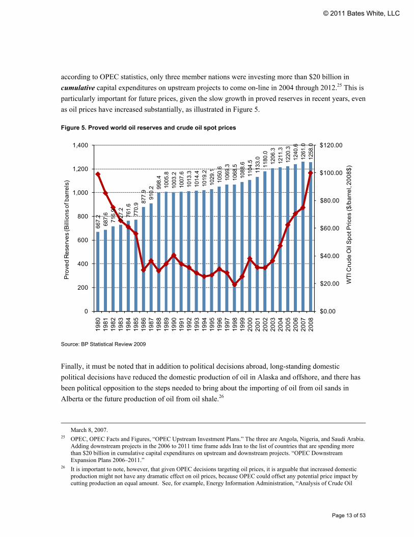
according to OPEC statistics, only three member nations were investing more than $20 billion in
cumulative capital expenditures on upstream projects to come on-line in 2004 through 2012.25 This is
particularly important for future prices, given the slow growth in proved reserves in recent years, even
as oil prices have increased substantially, as illustrated in Figure 5.
Figure 5. Proved world oil reserves and crude oil spot prices
Source: BP Statistical Review 2009
Finally, it must be noted that in addition to political decisions abroad, long-standing domestic
political decisions have reduced the domestic production of oil in Alaska and offshore, and there has
been political opposition to the steps needed to bring about the importing of oil from oil sands in
Alberta or the future production of oil from oil shale.26
March 8, 2007.
25 OPEC, OPEC Facts and Figures, “OPEC Upstream Investment Plans.” The three are Angola, Nigeria, and Saudi Arabia. Adding downstream projects in the 2006 to 2011 time frame adds Iran to the list of countries that are spending more than $20 billion in cumulative capital expenditures on upstream and downstream projects. “OPEC Downstream Expansion Plans 2006–2011.”
26 It is important to note, however, that given OPEC decisions targeting oil prices, it is arguable that increased domestic production might not have any dramatic effect on oil prices, because OPEC could offset any potential price impact by cutting production an equal amount. See, for example, Energy Information Administration, “Analysis of Crude Oil
667.
268
7.6
716.
972
7.2
761.
677
0.9 87
7.9
910.
2 998.
410
05.8
1003
.210
07.6
1013
.310
14.4
1019
.210
29.1
1050
.610
69.3
1068
.510
88.6
1104
.511
33.0
1180
.012
06.3
1211
.312
20.3
1240
.612
61.0
1258
.0$0.00
$20.00
$40.00
$60.00
$80.00
$100.00
$120.00
0
200
400
600
800
1,000
1,200
1,400
19
80
19
81
19
82
19
83
19
84
19
85
19
86
19
87
19
88
19
89
19
90
19
91
19
92
19
93
19
94
19
95
19
96
19
97
19
98
19
99
20
00
20
01
20
02
20
03
20
04
20
05
20
06
20
07
20
08
WT
I Cru
de
Oil
Sp
ot P
rice
s ($
/ba
rre
l, 2
00
8$
)
Pro
ved
Re
serv
es
(Bill
ion
s o
f ba
rre
ls)
© 2011 Bates White, LLC

Page 14 of 53
II.A.2. In Major Oil Producing Countries, Political Instability and Violence Reduce Output
In addition to its dependence on the political decision-making process in oil exporting nations, the
world supply of oil is reduced by war, terrorism, and guerrilla activity that are the result of political
instability or conflict. During the time period we analyzed, political instability and conflict in the
Middle East and in Nigeria, in particular, had a significant impact on oil production and the world
price of oil.
Tensions involving Iran have been associated with some of the highest oil prices in history, and the
easing of these tensions has been associated with the reduction in oil prices from their record high
levels. For example, the largest nominal increase in oil prices prior to the peak in 2008, $10.75 per
barrel, occurred on June 6, 2008,27 following the remark by an Israeli cabinet minister that Israel
might attack Iran.28 Other events involving Iran, ranging from a missile test to the easing of political
tensions, were associated with both increases and decreases in oil prices in July 2008, as is discussed
in the following section.
With respect to Iraq, extended periods of war over the past several decades have been associated with
dramatic reductions in Iraqi production of oil. The intervening years of relative peace were associated
with recovery in the levels of production. This is illustrated in Figure 6. Iraq’s 2008 production of
2,423 thousand b/d, following years of recovery from its low in 2003, is still only approximately 69%
of Iraq’s peak production of 3,489 thousand b/d in 1979 prior to the Iran-Iraq war.
As is discussed in more detail in the next section, politically motivated violence in the Niger Delta
reduced exports of Nigerian oil, and the news of such unrest was associated with increases in the
price of oil. The recurring violence, abductions of foreign workers, and sabotage of oil infrastructure
reduced output by 20%.29
Finally, in the spring of 2011, oil prices have risen amid concerns about the impact of unrest in Arab
countries on oil production and transportation.
Production in the Arctic National Wildlife Refuge,” May 2008.
27 It was the largest increase in relative terms since June 1996. 28 Another event on that day included comments by the head of Libya’s National Oil Corporation that the price of oil
would rise to $140 per barrel. A number of reports also cited a research note by Morgan Stanley that oil prices might spike to $150 per barrel as a result of strong demand in Asia (which as discussed below is fueled by government subsidies) and tight supplies in the United States. However, the Morgan Stanley forecast actually came out on May 28, 2008. See references in section IV, and Mark Shenk, “Oil Rises after Morgan Stanley Says Brent Oil May Reach $150,” Bloomberg, May 28, 2008. The price increase on May 28 was not large enough to be included in our analysis in section III.
29 Austin Ekeinde, “Three Foreign Oil Workers Kidnapped in Nigeria,” Reuters, Feb. 19, 2007.
© 2011 Bates White, LLC

Page 15 of 53
Figure 6. Iraqi oil production
Source: BP Statistical Review 2009
II.B. As a Nonrenewable Resource, Natural Factors Affect the Total Supply of Oil
While political decisions affect oil production in both the short term and the long term, oil is a
nonrenewable natural resource. As such, even though additional reserves no doubt remain to be
discovered, the total supply of oil is virtually fixed. The quantity of oil that can be extracted from a
given reservoir and the cost of extraction depend on the physical characteristics of the oil and the
reservoir, as well on as the available extraction technology.
The cost of developing new sources has increased dramatically in recent years, and new sources often
produce heavier grades of oil. New reserves of oil are expensive to bring to market; they tend to
consist of heavy oil and are more difficult to extract, because these new reserves are located in remote
areas, deep waters, or ultradeep waters. For example, at the Madrid World Petroleum Congress, BP’s
0
500
1,000
1,500
2,000
2,500
3,000
3,500
4,0001
96
5
19
67
19
69
19
71
19
73
19
75
19
77
19
79
19
81
19
83
19
85
19
87
19
89
19
91
19
93
19
95
19
97
19
99
20
01
20
03
20
05
20
07
Th
ou
san
ds
of b
arr
els
pe
r da
y
Start of Iran-Iraq War (September 1980)
Start of Persian Gulf War(August 1990)
Start of the Iraq War(March 2003)
© 2011 Bates White, LLC

Page 16 of 53
CEO Tony Hayward stated that the OECD will have to rely more on frontier areas such as oil sands,
heavy oil, and deepwater Mexico.30
Examples of such new sources include Alberta’s heavy oil sands, the Guará discovery in ultradeep
waters offshore Brazil, and Mexico’s deepwater offshore fields (which provide Pemex with many
financial and technological challenges).31 The largest addition to world reserves in this century has
been, as noted above, the heavy oil from the oil sands of Alberta. The EIA’s International Energy
Outlook 2009 reference case projects unconventional sources of oil, such as oil sands, oil shale,
ultraheavy crude, biofuels, and gas- or coal-to-liquids will account for 13 million barrels per day or
approximately 12% of world liquids production in 2030.32
At the same time that heavy oil is making up a larger share of world reserves and production, demand
for light and middle distillates has been growing faster than the demand for all grades of crude oil in
total.33 Refining heavy crude oil requires expensive investment in new refineries or upgrades to
existing refineries that require years to complete.34
II.C. The Demand for Oil is Dependent upon Both Political Decisions and Economic Factors
The discussion above has focused on the political and natural factors that affect the supply of oil. In
recent years, political events have contributed to an increase in demand for oil as well. As recent
events have shown, economic factors have also affected the demand for oil.
Many governments around the world provide subsidies for transport, agriculture, and other sectors to
spur economic activity or to curb inflation.35 These subsidies shield certain sectors from oil price
increases—notably in countries in which demand was growing most rapidly through mid-2008. As a
result, demand in these countries failed to respond to higher world prices.
Governments that currently or recently subsidized gasoline are predominantly in the Middle East and
Southeast Asia. These include China and countries in the former Soviet Union, along with some oil-
30 “Debate on High Oil Prices Moves to Madrid,” Platts Oilgram Price Report 86, no. 126, July 1, 2008. 31 See discussion in Energy Information Administration, International Energy Outlook 2009, Chapter 2, “Liquid Fuels.” 32 Id. 33 Jeff Mower, “Lots of Crude Available on Market, but Most of It Is Wrong Kind; Lack of Light, Sweet Barrels a
Fundamental Reason Behind Price Surge,” Platts Oilgram News, Nov. 1, 2007; and BP Statistical Review of World Energy, June 2009.
34 See, e.g., “Shell Scraps Plans for Refinery at Sarnia,” Toronto Star, July 9, 2008; “Marathon Detroit Heavy Upgrade Project;” or Mohan S. Rana, J. Ancheyta, S.K. Maity, G. Marroquin, “Comparison Between Refinery Processes for Heavy Oil Upgrading: A Future Fuel Demand,” International Journal of Oil, Gas, and Coal Technology 1, no. 3 (2008): 250–82.
35 Kevin Grey, “Chile Cenbank Says Fuel Subsidy Will Curb Inflation,” Reuters, June 19, 2008.
© 2011 Bates White, LLC

Page 17 of 53
producing countries in Africa and South America. The countries that currently or until recently have
subsidized gasoline and diesel fuel include: Algeria, Angola, Argentina, Azerbaijan, Bahrain,
Bangladesh, Belarus, Bolivia, Brunei, Burma (Myanmar), Chile, China, Cuba, Ecuador, Egypt,
Eritrea, Ethiopia, Gabon, Ghana, India, Indonesia, Iran, Jordan, Kuwait, Libya, Malaysia, Nepal,
Nigeria, North Korea, Oman, Pakistan, the Philippines, Qatar, Russia, Saudi Arabia, Singapore, Sri
Lanka, Syria, Taiwan, Trinidad and Tobago, Turkmenistan, United Arab Emirates, Venezuela,
Vietnam, and Yemen.36, 37 As recently as November 2006, more than 60% of the world’s population
was living in countries that subsidized the price of gasoline and diesel fuel.38 The largest countries
that subsidize fuel, in terms of their annual spending on fuel subsidies, have included China ($40
billion) and Indonesia ($20 billion).39, 40
In countries without subsidies, crude oil demand become stagnant or fell as global crude oil prices
climbed in 2007 and 2008. But in countries with subsidies, demand was largely unresponsive to price
changes. These political decisions maintain artificially high demand for crude oil. BP estimates that
countries with subsidies accounted for 96% of the world’s increase in oil consumption in 2007.41
It was not until the surge in crude oil prices that governments began to eliminate fuel subsidies as
they faced enormous budget shortfalls and mounting levels of public debt. China announced on June
19, 2008, that it would allow fuel prices to rise. According to press reports, this announcement
prompted a one day $4.75 (or 3.5%) decline in the WTI crude oil spot price.42 Between May and July
2008, a number of other governments, including India, Indonesia, and Iran scaled back subsidies and
allowed fuel prices to rise.43
The differences between countries in the pattern of demand growth and decline are consistent with
these observations. The demand for oil began falling in 2006 in the United States and in the OECD as
36 Federal Ministry for Economic Cooperation and Development, International Fuel Prices 2007, 5th ed. 37 Other countries not on this list have subsidies. For example, the United States has subsidized heating oil in the Northeast
for poor families, although this subsidy is not funded by the US government, but by the government of Venezuela. “Venezuela’s Chávez Promises Oil for Paraguay,” International Herald Tribune, Associated Press, Aug. 17, 2008.
38 US Census Bureau, International Data Base (IDB), 2008. 39 Keith Bradsher, “Fuel Subsidies Overseas Take a Toll on U.S.,” New York Times, July 28, 2008. 40 In addition, governments purchase and maintain fuel stockpiles. The US government held approximately 725 million
barrels of crude oil (as of October 19, 2009) in the Strategic Petroleum Reserve, http://www.spr.doe.gov/dir/dir.html. The US government temporarily suspended government purchases of crude oil to replenish the Strategic Petroleum Reserve in May 2008 in an attempt to slow rising fuel prices. “Bush Freezes Nation’s Emergency Oil Supply,” CNN Money, May 19, 2008, http://money.cnn.com/2008/05/19/news/economy/bush_spr/index.htm?section=money_news_economy.
41 Keith Bradsher, “Fuel Subsidies Overseas Take a Toll on U.S.,” New York Times, July 28, 2008. 42 Don Lee, “China to Raise Fuel, Electricity Prices; Global Oil Markets Take Notice,” Los Angeles Times, June 20, 2008. 43 Steve Hargreaves, “Bye-Bye Gas Subsidies,” CNNMoney, July 7, 2008,
http://money.cnn.com/2008/07/02/news/international/gas_subsidies/index.htm.
© 2011 Bates White, LLC

Page 18 of 53
a whole.44 World consumption of oil, however, did not decrease until the third quarter of 2008, when
it fell by 1.3% compared to the third quarter of the previous year. In that quarter, US demand for oil
fell by 8.8%, OECD demand as a whole fell by 4.5%, and demand by non-OECD countries continued
to rise by 2.9%.
Economic factors, including the price of oil and the overall state of the economy, have also affected
the demand for oil. The CFTC has pointed to the expansion of world economic activity by 5%
between 2004 and 2008, including robust economic growth in developing nations as well as
government oil subsidies, as reasons for growing global oil demand.45 Even before commodity prices
began falling in late summer 2008, prolonged high oil prices were a drag on consumer spending, as
heating and transportation costs became a larger share of total expenditures, resulting in a reduction in
demand. This phenomenon—termed “demand destruction”—was widely discussed in the first half of
2008.46
In fall 2008, the meltdown of financial markets diminished demand for oil. The collapse of stock
prices and housing prices and the rise in unemployment caused real and perceived wealth effects that
led to a substantial slowdown in consumer spending that was accompanied by falling energy prices.
The largest oil price declines ever recorded were fueled by concerns of a severe economic recession
and weak economic reports, as shown in the next section.
II.D. Foreign Exchange Fluctuations Affect the Dollar-Denominated Price of Oil
The discussion above has focused on some of the determinants of the physical supply and demand for
crude oil. Monetary factors, however, also affect the price of oil.
A key traded energy commodity is West Texas Intermediate (WTI) crude oil delivered to Cushing,
Oklahoma, and traded on the NYMEX as Light Sweet Crude Oil. It is the price of WTI that is used in
the analyses in the remainder of this paper, and this was the primary oil price that was referenced in
public discussions and CFTC investigations. The price of WTI is denominated in dollars. When the
value of the dollar falls, imported oil, which is the marginal source of supply for the United States,
becomes more expensive in dollars. The impact of the depreciating dollar is shown in Figure 7, which
44 EIA Short Term Energy Outlook, October 2009 and BP Statistical Review of World Energy, June 2009. 45 Interagency Task Force on Commodity Markets, “Interim Report on Crude Oil,” July 2008, (“Task Force, 2008”). 46 See, e.g., Alex Lawler, “Oil Slides Below $92 on U.S. Economic Concerns,” Reuters, Jan. 15, 2008,
http://www.reuters.com/article/2008/01/15/us-markets-oil-idUST3904820080115; Christian Weissner, “Oil Slumps on Dollar, Easing Supply Fears,” Reuters, April 29, 2008, http://uk.reuters.com/article/2008/04/29/us-markets-oil-idUKSYD3274320080429. For definition, see, Jerry Garrett, “Big Oil’s Tipping Point: Demand Destruction,” New York Times, Oct. 21, 2008.
© 2011 Bates White, LLC
Page 19 of 53
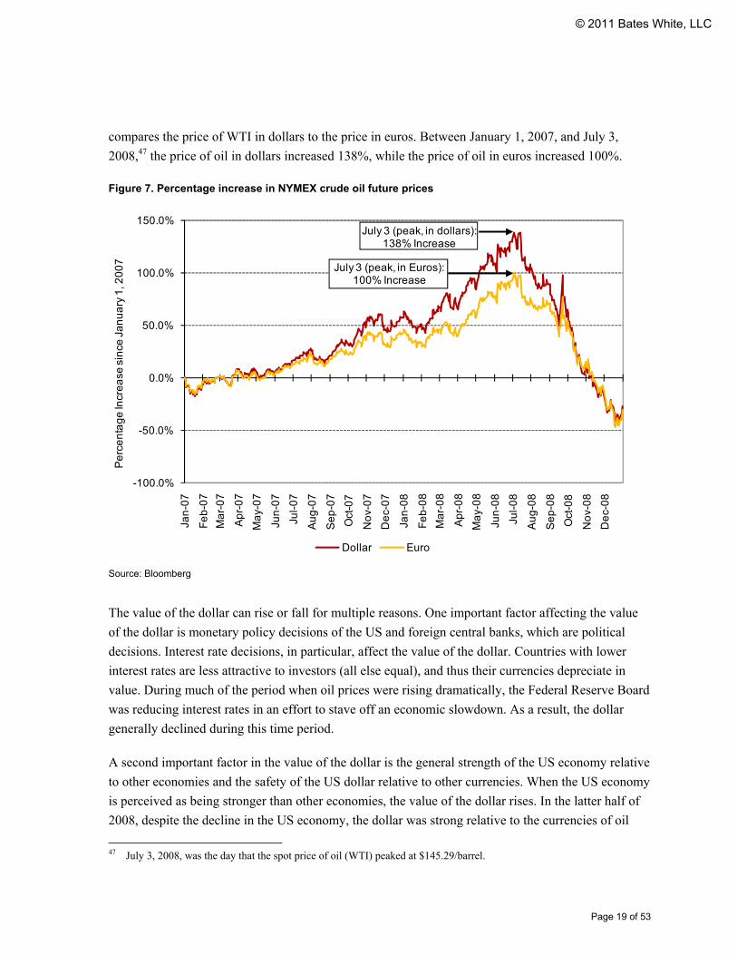
compares the price of WTI in dollars to the price in euros. Between January 1, 2007, and July 3,
2008,47 the price of oil in dollars increased 138%, while the price of oil in euros increased 100%.
Figure 7. Percentage increase in NYMEX crude oil future prices
Source: Bloomberg
The value of the dollar can rise or fall for multiple reasons. One important factor affecting the value
of the dollar is monetary policy decisions of the US and foreign central banks, which are political
decisions. Interest rate decisions, in particular, affect the value of the dollar. Countries with lower
interest rates are less attractive to investors (all else equal), and thus their currencies depreciate in
value. During much of the period when oil prices were rising dramatically, the Federal Reserve Board
was reducing interest rates in an effort to stave off an economic slowdown. As a result, the dollar
generally declined during this time period.
A second important factor in the value of the dollar is the general strength of the US economy relative
to other economies and the safety of the US dollar relative to other currencies. When the US economy
is perceived as being stronger than other economies, the value of the dollar rises. In the latter half of
2008, despite the decline in the US economy, the dollar was strong relative to the currencies of oil
47 July 3, 2008, was the day that the spot price of oil (WTI) peaked at $145.29/barrel.
-100.0%
-50.0%
0.0%
50.0%
100.0%
150.0%
Jan
-07
Fe
b-0
7
Ma
r-0
7
Ap
r-0
7
Ma
y-0
7
Jun
-07
Jul-
07
Au
g-0
7
Se
p-0
7
Oct
-07
No
v-0
7
De
c-0
7
Jan
-08
Fe
b-0
8
Ma
r-0
8
Ap
r-0
8
Ma
y-0
8
Jun
-08
Jul-
08
Au
g-0
8
Se
p-0
8
Oct
-08
No
v-0
8
De
c-0
8
Pe
rce
nta
ge
Incr
ea
se s
ince
Ja
nu
ary
1, 2
00
7
Dollar Euro
July 3 (peak, in dollars):138% Increase
July 3 (peak, in Euros):100% Increase
© 2011 Bates White, LLC

Page 20 of 53
exporting countries. Thus, the strength of the US dollar was one factor in the decline of oil prices in
late 2008.
II.E. Changes in Investment in Oil Futures and Options
As crude oil and gasoline prices climbed in 2007 and the first half of 2008, questions were raised in
public debates about the relationship between these price increases and financial investment in oil and
refined products. Similar questions were raised about the relationship between financial investment in
agricultural commodities and increases in the prices of these commodities. And more recently, in
2011, questions are being raised about the role of financial traders in the recent increase in oil prices.
In this section, we describe changes in commodity futures markets and we illustrate the extent to
which participation in the NYMEX oil market by financial investors has increased since 2000. The
CFTC has historically classified traders into two main categories: commercial (including commodity
swap dealers) and noncommercial traders. Until September 2009, the only reports that were publicly
available were for these two main classifications of traders, as well as the small nonreportable
positions category. As shown in Figure 8, commercial traders typically maintained a net short
position, consistent with hedging a long position, while over most periods, noncommercial traders
maintained a net long position.
© 2011 Bates White, LLC

Page 21 of 53
Figure 8. NYMEX crude oil futures price vs. reportable trader positions (January 2001–December 2008)
Source: CFTC, Commitments of Traders Reports
In addition to short or long outright positions, the spread positions of noncommercial traders in the
CFTC’s Large Trader Reporting System (LTRS) are also reported. Spread positions are comprised of
a long position in one contract month offset by a short position in another contract month. As open
interest in WTI futures and options has increased, noncommercial spread positions have increased
more than either commercial or noncommercial outright positions, as shown in Figure 8. Commercial
and noncommercial outright positions increased by approximately 100% between 2004 and 2008,
while noncommercial spread positions increased by more than 400%.48 The growth in spread
positions has been linked to the growth in hedge fund positions.49 According to the CFTC, the “vast
majority” of noncommercial traders entered into spread positions instead of taking either outright
long or outright short positions. Spread trading accounted for roughly 10% of the WTI market in 1995
and over 40% in 2008.50
48 The commercial and noncommercial outright positions are measured as the average of long and short positions. The
growth rate is calculated based on the average of all reported weeks during 2004 and 2008. 49 Michael S. Haigh, Jeffrey H. Harris, James A. Overdahl, and Michel A. Robe, “Market Growth, Trader Participation and
Derivative Pricing,” April 27, 2007, Working Paper, 2. 50 CFTC, “Staff Report on Commodity Swap Dealers & Index Trades with Commission Recommendations,” Sept. 2008,
0
200,000
400,000
600,000
800,000
1,000,000
1,200,000
1,400,000
1,600,000
1,800,000
$0
$20
$40
$60
$80
$100
$120
$140
$1602
00
1
20
02
20
03
20
04
20
05
20
06
20
07
20
08
Co
ntr
act
s o
f 1,0
00
Ba
rre
ls
Cru
de
Oil
Fu
ture
s P
rice
($
/bb
l)
NYMEX Futures Price ($/bbl, L-axis) Commercial Long (R-axis)Commercial Short (R-axis) Noncommercial Long (R-axis)Noncommercial Short (R-axis) Noncommercial Spread (R-axis)
© 2011 Bates White, LLC

Page 22 of 53
Within the commercial and noncommercial trader classifications, there are additional categories. The
four main categories of commercial traders historically have been: (1) Dealer/Merchants, (2)
Manufacturers, (3) Producers, and (4) Commodity Swap Dealers.51 The three most active categories
of noncommercial traders are: (1) Floor Brokers and Traders, (2) Hedge Funds (included in the
Managed Money Trader category), and (3) Non-registered Participants (NRPs).52 The
Dealer/Merchant, Manufacturer, and Producer categories are regarded as “traditional” commercial
traders, and swap dealers often hedge over-the-counter (OTC) transactions related to commodity
index funds.
The allocation of NYMEX crude oil positions between trader categories has changed in recent years,
with growth heavily concentrated in the noncommercial trader categories and commodity swap
dealers. For example, futures and futures-equivalent options positions held by hedge funds and
nonregistered participants grew from approximately 68,000 in 2000 to over 1 million in 2008, an
increase of 1,442%.53 The quantity of futures and futures-equivalent options contracts held by two
other categories of traders also increased significantly during this time period: contracts held by floor
brokers/traders increased by 454%, and contracts held by commodity swap dealers increased by
354%.
Part of the growth in swap dealer positions was attributed to investor interest in commodity index
funds (CIFs), which generally invest to track a particular commodity index and thus are long the
commodities in that index. Commodity swap dealers often serve as market makers on behalf of CIFs
and then hedge the risk that they have taken on in the futures markets. In 2008, it was estimated that
almost $9 out of every $10 of CIF investments were conducted through dealers that belonged to the
International Swaps and Derivatives Association.54
Institutional investors, such as pension and endowment funds, added CIFs to their portfolios in the
1990s and 2000s. For example, Netherlands-based Stichting Pensioenfonds ABP, the world’s largest
retirement fund, began investing in commodities in 1991. CalPERs, the California Public Employees
at 9.
51 The CFTC first published disaggregated COT reports in September 2009. The disaggregated reports include open interest for the following five categories: producer/merchant/processor/user, swap dealers, managed money, and other reportables, and nonreportable positions. In late October 2009, the CFTC made available publicly historical disaggregated reports that went back to June 13, 2006. However, the now-publicly available COT reports do not include the level of disaggregation that is available to the CFTC. Thus, much of the discussion in the remainder of this section is drawn from reports by researchers, including CFTC staff, with access to reports that are not public. Our analysis of the publicly available data is given in section IV.
52 Büyükşahin, Bahattin, Michael S. Haigh, Jeffrey H. Harris, James A. Overdahl, Michel A. Robe, “Fundamentals, Trader Activity, and Derivative Pricing,” EFA 2009 Bergen Meetings Paper, Dec. 4, 2008 (Büyükşahin, et al.), at 15.
53 Büyükşahin, et al. (2008), table 5. Büyükşahin, et al. classifies hedge funds (which aggregate Commodity Pool Operators, Commodity Trading Advisors, Associated Persons, and other Managed Money traders) and nonregistered participants as the primary financial trader categories.
54 Gene Epstein, “Commodities: Who’s Behind the Boom?” Barron’s, March 31, 2008.
© 2011 Bates White, LLC

Page 23 of 53
Retirement fund, began investing in commodities in 2007.55 CIFs were seen as a way to diversity
investment portfolios. CIFs were attractive because, historically, the growth in commodity returns has
been negatively correlated with the stock market, and in recent years, investors have sought exposure
to commodities to balance their portfolios. In addition, because commodity prices generally rise with
inflation, investors use CIFs as an inflation hedge.56
Work by Büyükşahin et al. (2008), using disaggregated CFTC data that is not publicly available,
shows substantial growth in NYMEX crude oil futures and futures-equivalent option open interest in
most trader categories. In particular, the growth in open interest between 2000 and 2008 was largest
for the noncommercial trader categories. Commodity swap dealers open interest increased from less
than 250,000 contracts in 2008 to well over 750,000 contracts in 2008. Hedge funds increased their
open interest from a very small amount in 2000 to between 500,000 and 750,000 contracts in 2008,
constituting the second large position among investor categories.57
In addition to the change in allocation between trader categories and the growth of spread positions,
the composition of maturities traded has changed. This is also illustrated in Büyükşahin et al.
(2008).The volume of trading in contracts with longer maturities increased substantially over the
2000–2008 period. The fastest growth rates occurred in the longer maturity categories. The growth in
longer-term maturities has been shown by Büyükşahin, et al. (2008) to be associated with increases in
the prices of nearby and longer maturity contracts. These enhance liquidity and price discovery as
well as the ability of traders to use longer-term positions to hedge.58
55 “CalPERS Gets Lured by the Sheen Of Oil, Gold and Timber,” Sept. 16, 2006, Financial Express,
http://www.financialexpress.com/news/calpers-gets-lured-by-the-sheen-of-oil-gold-and-timber/177827/0; “Calpers Jumps In, Commodity Rush Intensifies,” Bloomberg, Dec. 19, 2005, http://www.mosler.org/wwwboard/messages/3065.shtml; and “Capital Gold Group Report: Calpers - Largest U.S. Pension Fund - Bullish on Hard Assets,” Bloomberg, Feb. 28, 2008, http://www.thecapitalgoldgroup.com/2008/02/capital-gold-group-report-calp.html.
56 Interagency Task Force on Commodity Markets, “Interim Report on Crude Oil,” July 2008, at 9, 13. 57 See Büyükşahin, et al. (2008), table 5. 58 The econometric term for this comovement is cointegration. In particular, Büyükşahin, et al. found that the size of
positions held by commodity swap dealers, as well as hedge funds and nonregistered participants, led to increased cointegration between short-term and long-term oil futures prices. (Büyükşahin, et al. (2008), at 23, 28.)
© 2011 Bates White, LLC

Page 24 of 53
III. Econometric Analysis of Events Affecting Daily Changes in Oil Prices
In section II, we described the impact of factors that have a long- as well as a short-term impact on oil
prices. At any given point in time, however, specific events or new information might change
perceptions about the impact of these forces on oil supply and demand in both the short and long
terms, causing fluctuations in both the spot price and futures prices for oil. Given the availability of
storage, even changes in perceptions about supply and demand in the medium and long term will
affect near-term prices.
In section III, we examine whether new market information and specific world events were associated
with major changes in the price of oil during 2007 and 2008. While there has been much debate over
causes of the historic movements in oil prices before and after the peak of oil prices in 2008, to our
knowledge, there has not been an examination on a day-by-day basis of the events associated with oil
price increases and decreases during this period.
Based on our econometric analysis, we find that, during approximately the year and a half that oil
prices were trending upward (through July 14, 2008), political instability and acts of violence were
the dominant fundamental events associated with daily oil price changes. In particular, peak oil prices
and the largest daily price increases coincided with escalating nuclear tensions with Iran, including a
threat by an Israeli cabinet minister to attack Iranian enrichment facilities. Furthermore, during the
period through July 14, 2008, while negative economic news temporarily reduced oil prices,
perceptions of weaker energy demand did not result in a sustained decrease in oil prices. In addition,
we find that news reports of speculative activity or financial trading did not have a significant impact
on large price movements during the period through July 14, 2008.
Beginning on July 15, 2008, tensions with Iran began to subside as the United States entered into
diplomatic talks with Iran. This period was marked by a significant reduction in oil prices—the
largest three-day decline in our sample ($15.89 per barrel). The decline in oil prices during the
summer of 2008 also coincided with the beginning of a decrease in violence in Iraq.59 Importantly, by
late summer and fall 2008, it was widely recognized that the world economy had entered into the
most severe downturn since the Great Depression. It is not surprising that during the late-July to
December 2008 time frame, economic factors dominated the fundamental events associated with
daily oil price changes. Nonetheless, even during this period of severe economic contraction, political
instability and violence—such as acts of warfare between Israel and Hamas in late December—were
as important as in the prior period in explaining large upward movements in oil prices.
59 “Pentagon: Violence Down in Iraq Since ‘Surge,’” CNN, June 23, 2008, http://articles.cnn.com/2008-06-
23/world/iraq.security_1_troop-deaths-sadr-city-iraqi-troops?_s=PM:WORLD.
© 2011 Bates White, LLC

Page 25 of 53
III.A. Data and Methodology
To identify events associated with oil price movements in 2007 and 2008, we examined trade and
business press reports for the 197 days oil prices increased or declined by 2% or more.60 These days
account for 39% of the trading days during this two-year period and 74% of the variation in crude oil
prices.61 We divide the events into three major categories—political, economic, and natural events—
with the following subcategories:62
Political events and governmental decisions
Announcements by OPEC officials and other governmental decisions impacting oil
ownership and production
Monetary policy actions
Other political events, including political instability, acts of violence, and changes in demand
subsidies abroad63
Economic factors
Inventory announcements
News about financial trading, including speculation or alleged market manipulation
Other economic events
Natural events that have the potential to temporarily affect the price of oil
Extreme weather events, such as hurricanes, that damage or disrupt offshore production or
refinery processing
Changes in temperature that impact heating demand
We divided the 2007 and 2008 time frame into the pre- and post-July 14, 2008, periods.64 In the pre-
July 14, 2008, period, there were 66 days with price increases of 2% or more and 53 days with
60 The primary news sources we relied on were Bloomberg, CNN Money, the Guardian, the New York Times, and Reuters.
Cutler, Poterba, and Summers (1989) used several approaches to examine the impact of news events and macroeconomic news on stock market prices. One of their approaches was to identify the New York Times accounts of fundamental factors that affected stock prices on the 50 days with the largest one-day returns on the S&P Composite Stock Index between 1946 and 1989. David Cutler, James Poterba, and Lawrence Summers, “What Moves Stock Prices?” Journal of Portfolio Management, Spring 1989; 15, 3; 4.
61 The variation is measured as the sum of the absolute value of daily oil price movements. The 74% of variation is comprised of 71% of price increases and 77% of price decreases. The one-day price change is the percentage change in the NYMEX futures crude oil price. When we compare the analysis for the 197 days with changes of 2% or more with the 148 days with changes of 2.5% and the 114 days with 3% or more, the results are similar.
62 The remaining events, listed as “Other,” generally include news about refinery or pipeline availability. 63 This category is dominated by political instability and violence or warfare. However, the few instances in which
countries reduced demand subsidies did contribute to a reduction in world oil prices.
© 2011 Bates White, LLC

Page 26 of 53
decreases of 2% or more. In the post-July 14, 2008, period there were 26 days with price increases
and 52 days with decreases of 2% or more. It is not surprising that there were more days with price
increases than decreases in the period up until July 14, 2008, while the opposite was true for the
period after July 14, 2008.
The types of events that dominated the news and that were associated with large changes in oil prices
in the two periods differed in a manner that was not unexpected. During the earlier period, escalating
political conflict in the Middle East and other oil producing regions contributed to numerous price
increases that were not offset by subsequent price declines. While there was weak economic news, its
downward impact only temporarily lowered oil prices. During the later period, the collapse of
financial markets and the global economy combined with political uncertainty domestically over the
US bailout package was associated with the largest price declines ever, which were not offset by price
increases.
For example, on April 23, 2007, oil prices increased by $2.51. This increase was associated with
political events that raised global supply concerns. Venezuela prepared to nationalize four large heavy
oil projects to the detriment of private oil companies, and this was expected to reduce investment and
lead to a decline in production. On the same day, international observers disputed election results in
Nigeria, highlighting the threat of instability in the world’s eighth largest exporter after attacks by
militants had shut about one-fifth of oil production.65 By contrast, on July 31, 2008, oil prices fell by
$2.69. This decline was attributed to weak economic news bolstering concerns about shrinking US
energy demand. On that morning, a US Labor Department report showed a large increase in jobless
claims, and a US Bureau of Economic Analysis report showed that GDP grew at a weaker-than-
expected pace in the second quarter of 2008.66 Both of these reports were consistent with a reduction
in energy demand. The events that occurred on these two days illustrate the differences between the
general types of events driving oil price movements before and after July 14, 2008.
Even the news associated with large price increases differed in the two time periods. The largest
single day increase in oil prices pre-July 14, 2008—which occurred on June 6, 2008—was associated
with a falling dollar and a threat by an Israeli Cabinet minister of an “unavoidable” attack on Iranian
64 We used a Chow Test to detect the presence of a structural break across time periods in the model, selecting July 15,
2008, to mark the easing of political tensions in the Middle East and the transition period into the global economic recession.
65 Brian Ellsworth, “Venezuela Takeover May Harm Orinoco Oil Projects,” Reuters, April 23, 2007, http://uk.reuters.com/article/2007/04/23/uk-orinoco-venezuela-takeover-idUKN2328733320070423; Janet McBride, “Oil Climbs Above $67 after Nigeria Poll,” Reuters, April 23, 2007, http://www.reuters.com/article/2007/04/23/us-markets-oil-idUSSYD33365520070423.
66 Matthew Robinson, “Oil Drops 2 Percents, Caps Biggest Monthly Loss Since ’04,” Reuters, July 31, 2008, http://www.reuters.com/article/2008/07/31/us-markets-oil-idUST14048520080731; Catherine Clifford, “Stocks Take a Tumble,” CNNMoney, July 31, 2008, https://www.ccmg.com/Newsroom/cnn%20money%207.31.08.pdf.
© 2011 Bates White, LLC

Page 27 of 53
nuclear sites.67 This day also coincided with a perceived reduction in demand as a result of a bearish
unemployment report, which would have been likely to reduce the price of oil or limit the upward
price movement attributable to other events. In the post-July 14, 2008 period, the largest single-day
increase in oil prices—which occurred on September 22, 2008—was associated with reported
expectations of stronger demand, a weaker dollar, and inflation as a consequence of the bailout plan
announced over the weekend, as well as falling stock prices. Events on this day also included the
expiry of the October 2008 NYMEX futures contract, the reported launching of an investigation by
the CFTC into the possibility of market manipulation, reported moves by an unidentified hedge fund
to cover short positions, and increases in other commodity prices.68
The econometric methodology we used to estimate the proportion of oil price movements that can be
attributed to different types of news events is as follows. We regress the one-day percentage change
in the NYMEX crude oil futures price on a set of dummy variables that correspond to the
subcategories of events that occurred on a given day:
1 2 3 4 5 6
7 8 9 10 11 12
13 14 15 16 17
Price Return = FED FED OPEC OPEC POL POL
EXTR EXTR ECO ECO INV INV
SPC SPC NAT NAT OT
t t t t t t t
t t t t t t
t t t t
α α α α α αα α α α α αα α α α α
+ − + − + −
+ − + − + −
+ − + −
+ + + + +
+ + + + + +
+ + + + + 18H OTHt t tα ε+ −+ +
where FED denotes announcements or monetary policy actions by the Federal Reserve, OPEC
announcements by OPEC officials, POL political events, EXTR extreme political events, ECO
economic factors, INV inventory announcements, SPC events related to speculation or financial
trading, NAT natural or weather events, and OTH other events. Each independent variable is given a
value of one if an event in that particular subcategory occurred on that day, and it is given a zero
otherwise.69 We allow more than one type of event to affect oil prices on any given day, and we allow
for those events to have either a positive or negative effect. The estimated parameters are allowed to
vary depending on whether particular events would be expected to increase or decrease prices. We
estimated the regression separately for the pre- and post-July 14, 2008, periods. The coefficients
67 Dan Williams, “Israel to Attack Iran Unless Enrichment Stops: Minister,” Reuters, June 6, 2008,
http://www.reuters.com/article/2008/06/06/us-israel-iran-mofaz-idUSL0625195820080606. 68 Stevenson Jacobs, “Oil Makes Biggest Single-Day Price Jump Ever,” Associated Press, Sept. 22, 2008,
http://thehour.com/register/?storyid=421389. 69 In addition to the subcategories listed above, we found that in each time period there was one extremely large price
movement associated with unusual news events of war or threats of war. In the earlier time frame, the extreme event was the threat described above by an Israeli cabinet minister to attack Iran. It occurred during a time of heightened tensions between Iran and other nations over Iran’s nuclear program. In the later time frame, the extreme event was the war between Israel and Hamas in the Gaza strip. Source: Julia Kollewe, “Oil and Gold Prices Sharply Higher on Gaza Fighting,” Guardian, Dec. 29, 2008. These events had a much larger affect on oil prices than other events in the “Other Political” event subcategory, and thus they were given their own dummy variable.
© 2011 Bates White, LLC

Page 28 of 53
represent the average change in oil prices associated with each subcategory of events, taking into
account the other events occurring on each day.
III.B. Results
We applied the model, which included all the categories of fundamental events we identified, to both
time periods. The results are given in Figure 9. Figure 9 is divided into two panels. The first panel
provides results for the first period (January 1, 2007, through July 14, 2008) in which oil prices were
generally increasing. The second panel provides results for the second period (July 15 through
December 31, 2008) in which oil prices were generally decreasing.
The first two lines in each panel (labeled “Price Response (%)”) give the parameter estimates, which
can be interpreted as the average percentage price increase or decrease associated with each
subcategory of event, taking into account the other types of events that occurred.70 The second two
lines (labeled “Number of News Events”) give the number of times the dummy variable for each type
of event took on the value one. The calculations are differentiated by whether the event would have
been expected to increase or decrease prices. The third three lines (labeled “Percentage of Predicted
Price Change Explained”) give the percentage of price changes explained by the model that were
attributable to each subcategory, again differentiated by whether the event was expected to have
increased or decreased prices, and combined.71 The last line in each panel (labeled “Percentage of
Actual Price Change Explained by Model”) gives the percentage of the actual price change that was
explained by the model.72
During the period from January 1, 2007, to July 14, 2008, while oil prices were generally increasing,
the model explains 87% of the price movements on large price change days. Of the categories of
events, political events had the largest effect. Based on the explained price movement, 56% of price
changes were attributable to political events. Of this 56%, the majority was attributable to political
70 The significance of the parameters is denoted by the number of asterisks (*). Three asterisks denote significance at the
1% level, two at the 5% level, and one at the 10% level. 71 The percentage of predicted price change explained was calculated as the total dollar amount of oil price changes
attributed to each subcategory divided by the sum of all price movements predicted by the model. The price change in dollars for a given day attributed to each subcategory was estimated by multiplying the subcategory coefficient α by the lagged price if an event in that subcategory occurred on a particular day, because the estimated parameters can be interpreted percentage changes. The total dollar amount attributed to each subcategory was calculated as the sum of individual daily price changes.
72 The percentage of actual price change explained by the model was calculated as the sum of the absolute value of all price movements predicted by the model divided by the sum of the absolute value of all one-day price changes in the sample—the period from 2007 to 2008.
© 2011 Bates White, LLC

Page 29 of 53
instability or acts or threats of violence or war, which were included in the “Other Political” or
“Extreme” event categories. This was particularly true of the upward price movements.73
Approximately 31% of price movements can be explained by economic events (including inventory
reports), and 12% can be explained by natural events. During this time period, all the subcategories
except for the “Speculation” and “Other” subcategories were significant in explaining either upward
or downward price movements. 74
73 The lifting of or reduction in demand subsidies that were included in the “Other Political” category had some impact to
reduce prices. If the model is estimated without the five instances of reduction of demand subsidies, the percentage of price reduction explained by the “Other Political” subcategory falls from 28% to 21%.
74 We also estimated a model in which only the variables that were significant in the base model were retained. The same general results regarding the percentage of price movements explained by subcategory and overall were maintained.
© 2011 Bates White, LLC

Draft—Preliminary work product
Page 30 of 55
Figure 9. Effect of Events on Day-to-Day Price Changes
Natural OtherFed Policy OPEC Other Political Extreme Economy Inventory Speculation Weather Uncategorized
+ Events 0.949* 1.312** 2.269*** 10.147*** 1.634*** 1.761*** 0.693 1.121*** -0.026 - Events -0.839 -1.735*** -1.944*** -1.735*** -2.257*** -0.217 -1.885*** -0.700
+ Events 14 9 39 1 11 17 13 14 10 - Events 11 10 20 0 16 10 6 16 4
+ Events 7.4% 5.3% 43.5% 7.5% 9.3% 15.5% 4.3% 7.3% -0.1% - Events 6.6% 11.6% 27.6% 0.0% 20.4% 13.0% 0.8% 18.6% 1.4%All Events 7.1% 8.0% 36.5% 4.2% 14.2% 14.4% 2.7% 12.2% 0.7%
Percent of Actual Price Change Explained by Model
All Events 87.0%
Natural OtherFed Policy OPEC Other Political Extreme Economy Inventory Speculation Weather Uncategorized
+ Events 1.816 2.645* 3.123*** 6.126*** 3.145* 2.689** 10.719*** 0.404 7.847*** - Events 1.419 -2.017 -2.990** -4.279*** -2.536* -1.706
+ Events 5 14 25 1 7 6 1 5 2 - Events 2 6 14 0 44 10 0 5 0
+ Events 4.5% 15.1% 42.9% 1.6% 11.7% 9.0% 7.9% 1.5% 5.7% - Events -1.9% 4.8% 20.6% 0.0% 64.3% 7.9% 0.0% 4.2% 0.0%All Events 2.9% 8.7% 28.8% 0.6% 42.4% 8.1% 3.1% 3.1% 2.2%
Percent of Actual Price Change Explained by Model
All Events 89.3%
Political Economic
Political Economic
Price Response (%)
Number of News Events
Percent of Predicted Price Change Explained
Jan 1, 2007 to Jul 14, 2008
Jul 15, 2008 to Dec 31, 2008
Price Response (%)
Number of News Events
Percent of Predicted Price Change Explained
© 2011 Bates White, LLC

Page 31 of 53
In the second half of 2008, after July 14, oil prices fell as political tensions in the Middle East eased
and the global economic downturn began to reduce energy demand. The events in this time period
that were associated with large daily oil price changes were predominately economic events
(including inventory reports and allegations of speculation). Overall, the model explains 89% of the
large daily price changes. Of the explained price changes, 54% were attributable to economic events.
Political events explained approximately 41% of price movements, and natural events explained only
3% of large daily price changes.
Not surprisingly, political events had more of an upward than downward influence, and economic
events had more of a downward than upward influence. As a result, when looking at events expected
to cause an upward movement, approximately 64% of upward movements were attributable to
political events during both the first and second period. However, because 72% of downward price
movements were attributable to news about economic events during the last half of 2008, economic
events explained the majority of positive and negative price movements considered together—
approximately 54% of the total.
The only categories that were not significant in explaining either upward or downward price
movements were Federal Reserve policy and weather events. The category “Speculation” was
significant in the second half of 2008 but not in the pre-July 14, 2008, period. The only event during
the post-July 14, 2008, time period that was categorized as “Speculation” occurred on September 22,
2008, and included the settlement of the October 2008 NYMEX futures contract, the reported
launching of an investigation by the CFTC into the possibility of market manipulation, and reported
moves by an unidentified hedge fund to cover short positions.
© 2011 Bates White, LLC

Page 32 of 53
IV. The Role of Financial Trading
As crude oil and gasoline prices climbed in 2007 and the first half of 2008, questions were raised in
public debates about the relationship between these price increases and financial investment in oil and
refined products. Similar questions were raised about the relationship between financial investment in
agricultural commodities and increases in the prices of these commodities. In 2011, as oil prices
climb above $100/bbl and gasoline prices exceed $4 per gallon, the same concerns are being raised.
In this section, we examine the relationships among oil prices and the financial positions of three
groups of traders over four different periods. We are unable to find support for Granger causation of
oil prices by financial traders or “speculators” (trader categories of swap dealers and managed money
traders) during the “price run-up” period during which most concern was expressed. We find,
however, that the producer-merchant category of traders had positive a long-run Granger causality
relationship with price during the run-up period. We find evidence of nonlinear Granger causality of
price by swap dealer positions during the “stable” period of 2006 and 2007 and long-run Granger
causality during the “recovery” period of 2009. In addition, particularly during the price recovery
period, we find that there were complex relationships among the positions of trader groups and with
the price of oil. Finally, during both the “run-up” and “recovery” period, we find that managed money
positions adjusted to (or are Granger caused by) deviations from the long-run equilibrium relationship
between price and other trader group positions.
IV.A. Data
As described in more detail in section II, the CFTC has historically classified traders into two main
categories: commercial (including commodity swap dealers) and noncommercial traders. Until
September 2009, the only reports that were publicly available were for these two main classifications
of traders, as well as the small nonreportable positions category. As shown in section II, commercial
traders typically maintained a net short position, consistent with hedging a long position, while over
most periods, noncommercial traders maintained a net long position.
In addition to short or long outright positions, the spread positions of noncommercial traders in the
CFTC’s Large Trader Reporting System (LTRS) were also reported. Spread positions are comprised
of a long position in one contract month offset by a short position in another contract month. As open
interest in WTI futures and options increased, noncommercial spread positions increased more than
either commercial or noncommercial outright positions, as shown in section II. Commercial and
noncommercial outright positions increased by approximately 100% between 2004 and 2008, while
© 2011 Bates White, LLC

Page 33 of 53
noncommercial spread positions increased by more than 400%.75 The growth in spread positions has
been linked to the growth in hedge fund positions.76 According to the CFTC, the “vast majority” of
noncommercial traders enter into spread positions instead of taking either outright long or short
positions. Spread trading accounted for roughly 10% of the WTI market in 1995, and over 40% in
2008.77
Within the commercial and noncommercial trader classifications, there are additional categories. The
CFTC first published disaggregated COT reports in September 2009. The disaggregated reports
included open interest for the following five categories: producer/merchant/processor/user, swap
dealers, managed money, and other reportables, and nonreportable positions. In late October 2009,
the CFTC made available to the public historical disaggregated reports that went back to June 13,
2006. However, the COT reports made public in 2009 did not include the level of disaggregation that
is available to the CFTC.
In our analysis reported below, we analyze the relationship between and among the price of oil78 and
the corresponding net positions of the three main categories of traders: producer-merchant, swap
dealers, and managed money traders. These variables for the period of analysis are shown in Figure
10. In our analysis, we applied a logarithmic transformation to the oil price series.79 Thus, the change
in prices should be interpreted as a percentage change.
75 The commercial and noncommercial outright positions are measured as the average of long and short positions. The
growth rate is calculated based on the average of all reported weeks during 2004 and 2008. 76 Michael S. Haigh, Jeffrey H. Harris, James A. Overdahl, and Michel A. Robe, “Market Growth, Trader Participation and
Derivative Pricing,” April 27, 2007, Working Paper, 2. 77 CFTC, “Staff Report on Commodity Swap Dealers & Index Trades with Commission Recommendations,” Sept. 2008,
at 9. 78 The NYMEX prompt-month futures price, reported by Bloomberg. 79 This is a standard transformation and is consistent with the methods used in sections III and V as well. In addition, the
logarithmic transformation removes the nonlinearity in the oil price series that increased nearly exponentially over the course of our sample period.
© 2011 Bates White, LLC

Page 34 of 53
Figure 10. Crude oil futures and options combined net positions of disaggregated traders
Source: COT Reports, CFTC
IV.B. Methodology and Results
We employed Granger causality tests to analyze the lead and lag relations among oil prices and the
financial positions in a multivariate system. Büyükşahin and Harris (2011) studied similar issues and
used similar econometric techniques .80 These authors used CFTC proprietary data that broke
noncommercial positions into more detailed trader groups. Their data were also at a higher frequency
(daily) than the publicly available data that we analyzed here. These authors performed an extensive
series of Grange causality tests and were unable to detect any evidence that the financial positions
Granger caused oil prices.
In addition to different data sources and sample periods, our analysis differs from Büyükşahin and
Harris (2011) in other major aspects. First, they reported on only the bivariate relationships between
oil prices and financial positions; our multivariate models allowed us to also examine the 80 Bahattin Büyükşahin and Jeff Harris, “Do Speculators Drive Crude Oil Futures Prices?” Energy Journal 32, no. 2
(2011): 167–202.
-250,000
-200,000
-150,000
-100,000
-50,000
0
50,000
100,000
150,000
200,000
250,000
$0
$20
$40
$60
$80
$100
$120
$140
$160Ju
n-0
6
Au
g-0
6
Oct
-06
De
c-0
6
Fe
b-0
7
Ap
r-0
7
Jun
-07
Au
g-0
7
Oct
-07
De
c-0
7
Fe
b-0
8
Ap
r-0
8
Jun
-08
Au
g-0
8
Oct
-08
De
c-0
8
Fe
b-0
9
Ap
r-0
9
Jun
-09
Au
g-0
9
Oct
-09
Co
ntr
act
s o
f 1,0
00
ba
rre
ls
$/b
bl
Oil Price (L-axis) MM net (R-axis)
© 2011 Bates White, LLC

Page 35 of 53
relationships among financial positions of different trader groups. Second, we split our samples into
four different subperiods, according to the behavior of the oil prices, and we analyzed each period
separately. While sample splitting necessarily reduces the amount of data for analysis, the results we
find suggest that there were meaningful differences across these subperiods. Third, in addition to the
standard linear Granger causality tests, we also applied a nonparametric Granger causality test to
detect potentially nonlinear lead and lag relationship. To the best of our knowledge, no such tests
have been performed in our context before.
It is important to point out that Granger causality is not equivalent to a structural causal relation. It is
rather a statistical measure of whether the movements in one variable lead the movements in the
others. The concept of Granger causality is still useful, however, because without Granger causality
(precedence in time), it is generally acknowledged that a causal relation does not exist.81
Because Granger causality is known to be sensitive to the choice of variables in the system, we
believe that our multivariate system approach allowed us to better detect and understand the complex
relations between oil prices and financial variables. But, consistent with previous studies, we focused
only on the so-called one-step-ahead Granger causality in this paper. It is well known that Granger
causality is more intricate in a multivariate system, because one-step-ahead Granger causality does
not imply multiple-step-ahead Granger causality. Dufour and Renault (1998)82 and Lütkepohl and
Burda (1997)83 provide discussions on this topic, which we leave for future research.
IV.B.1. Preliminary Tests for Nonstationarity
Visually it is evident that oil prices have experienced four major episodes in our sample. In our
analysis, we divided the sample in the following way, as illustrated in Figure 11:
1. A period of relatively stable prices from June 13, 2006, to June 19, 2007 (the “stable period”)
2. A price run-up period from June 19, 2007, to July 15, 2008 (the “run-up period”)
3. A downturn period from July 15, 2008, to February 17, 2009 (the “downturn period”)
4. A recovery period from February 17, 2009, to October 31, 2009 (the “recovery period”)
81 See Halbert White and Xun Lu, “Granger Causality and Dynamic Structural Systems,” Journal of Financial
Econometrics 8, no. 2 (2010): 193–243 for a recent advance regarding the relation between Granger causality and structural causality.
82 J. M. Dufour and E. Renault, “Short Run and Long Run Causality in Time Series: Theory,” Econometrica 66 (1998): 1099–1125.
83 H. Lütkepohl and M. M. Burda, “Modified Wald Tests under Nonregular Conditions,” Journal of Econometrics 80 (1997): 223–39.
© 2011 Bates White, LLC

Page 36 of 53
It is of interest to determine whether the relationship between the positions of the major trader groups
and the price of oil differed within each of these time periods. Thus, we conducted our analysis on
these four subsamples.
Figure 11. Subperiod definition
Source: COT Reports, CFTC
We performed the DF-GLS test proposed by Elliott et al. (1994) 84 over these subsamples. Figure 12
contains the results of these tests. Except for the fact that the MM and SD net positions were
stationary over the stable period, the position series and oil price were nonstationary in all other cases.
84 Graham Elliott, et al., “Efficient Tests for an Autoregressive Unit Root,” Econometrica 64, 1996, 813–36. This
procedure is equivalent to a t-test in a standard ADF (Augmented Dickey Fuller) regression of the “GLS-detrended” time series. To select the lag order to construct the test, we used the modified Akaike Information Criterion (MAIC) proposed by Serena Ng and Pierre Perron, “Lag Length Selection and the Construction of Unit Root Tests with Good Size and Power,” Econometrica 69, 2001, 1519–1554. It has been shown in the literature that these procedures jointly provide both power and size improvement over the traditional ADF test. Standard textbooks provide details of these methods.
-250,000
-200,000
-150,000
-100,000
-50,000
0
50,000
100,000
150,000
200,000
250,000
$0
$20
$40
$60
$80
$100
$120
$140
$160
Jun
-06
Au
g-0
6
Oct
-06
De
c-0
6
Fe
b-0
7
Ap
r-0
7
Jun
-07
Au
g-0
7
Oct
-07
De
c-0
7
Fe
b-0
8
Ap
r-0
8
Jun
-08
Au
g-0
8
Oct
-08
De
c-0
8
Fe
b-0
9
Ap
r-0
9
Jun
-09
Au
g-0
9
Oct
-09
Co
ntr
act
s o
f 1,0
00
ba
rre
ls
$/b
bl
Oil Price (L-axis) MM net (R-axis)
Stable period Run-up period Downturn period
Recovery period
© 2011 Bates White, LLC
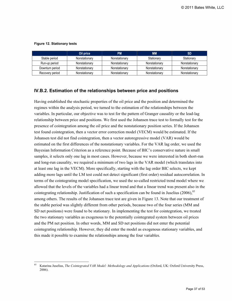
Page 37 of 53
Figure 12. Stationary tests
Oil price PM MM SD Stable period Nonstationary Nonstationary Stationary Stationary Run-up period Nonstationary Nonstationary Nonstationary Nonstationary
Downturn period Nonstationary Nonstationary Nonstationary Nonstationary Recovery period Nonstationary Nonstationary Nonstationary Nonstationary
IV.B.2. Estimation of the relationships between price and positions
Having established the stochastic properties of the oil price and the position and determined the
regimes within the analysis period, we turned to the estimation of the relationships between the
variables. In particular, our objective was to test for the pattern of Granger causality or the lead-lag
relationship between price and positions. We first used the Johansen trace test to formally test for the
presence of cointegration among the oil price and the nonstationary position series. If the Johansen
test found cointegration, then a vector error correction model (VECM) would be estimated. If the
Johansen test did not find cointegration, then a vector autoregressive model (VAR) would be
estimated on the first differences of the nonstationary variables. For the VAR lag order, we used the
Bayesian Information Criterion as a reference point. Because of BIC’s conservative nature in small
samples, it selects only one lag in most cases. However, because we were interested in both short-run
and long-run causality, we required a minimum of two lags in the VAR model (which translates into
at least one lag in the VECM). More specifically, starting with the lag order BIC selects, we kept
adding more lags until the LM test could not detect significant (first order) residual autocorrelation. In
terms of the cointegrating model specification, we used the so-called restricted trend model where we
allowed that the levels of the variables had a linear trend and that a linear trend was present also in the
cointegrating relationship. Justification of such a specification can be found in Juselius (2006),85
among others. The results of the Johansen trace test are given in Figure 13. Note that our treatment of
the stable period was slightly different from other periods, because two of the four series (MM and
SD net positions) were found to be stationary. In implementing the test for cointegration, we treated
the two stationary variables as exogenous to the potentially cointegrated system between oil prices
and the PM net position. In other words, MM and SD net positions did not enter the potential
cointegrating relationship. However, they did enter the model as exogenous stationary variables, and
this made it possible to examine the relationships among the four variables.
85 Katarina Juselius, The Cointegrated VAR Model: Methodology and Applications (Oxford, UK: Oxford University Press,
2006).
© 2011 Bates White, LLC

Page 38 of 53
Figure 13. Results of Johansen tests
Sample Cointegrating rank VAR Lag order Stable period 1 2 Run-up period 1 2 Downturn period 0 2 Recovery period 1 3
We find that there was one cointegrating vector among these variables over the run-up and the
recovery period, and that there was no cointegration over the downturn period.
Based on the Johansen tests, we estimated the lead-lag or Granger causality relationships between the
variables by using a VEC model, except for the downturn period. For the downturn period, we used a
stationary VAR model in which nonstationary variables were first differenced. More specifically, a
typical equation for the oil price in a VEC system is the following:
1 0 1 1 2 1 3 1 4 1 5
1 11 1 1 1
Oil ( Oil PM MM ( 1))
Oil PM MM SD ,
t t t t t
p p p p
i t i i t i i t i t ti i i i
SD tφ α δ δ δ δ δ δ
θ β λ γ ε
− − − −
− − − −= = = =
Δ = + + + + + + −
+ Δ + Δ + Δ + Δ +
where Δ is the first difference operator (i.e., Oilt – Oilt-1).
0 1 1 2 1 3 1 4 1 5Oil PM MM ( 1)t t t tSD tδ δ δ δ δ δ− − − −+ + + + + − is the so-called error correction term. It
measures the deviations from the long-run equilibrium among these variables. The parameters of the
error correction term describe the long-run equilibrium relationship among the variables.86 The
coefficient α describes the response of oil prices to long-run disequilibrium among these variables.
The response of oil prices to the short-run movements of the explanatory variables is given by θ, β, λ,
and γ .
Figure 14 illustrates graphically the direction of statistically significant Granger causality among the
variables.
86 δ4 is the slope of the time trend in the cointegration vector; this assumes that trends in the levels of the data are linear.
© 2011 Bates White, LLC

Page 39 of 53
Figure 14. Illustration of Granger causality results
Stable Period (VECM)
Run-up Period (VECM)
Downturn (VAR)
No relationships are found to be significant.
Recovery (VECM)
Notes
The dotted arrows describe the significant short-run relationships identified in the VAR-in-difference and VECM models. The dashed arrows describe the significant relationship between the equilibrium error (the error correction term) and the variable. The solid arrows describe the significant long-run cointegration relationships identified in VECM models.
The directions of the dotted arrows indicate the direction of short-run Granger causality in the VAR and VECM models. The directions of the solid arrows in ECM are determined by which variables are weakly exogenous. The negative/positive signs are determined by whether two variables have the same/different signs in cointegrating vectors. For example, in a four-variate model, if the cointegration vector of Price, MM, PM, and SD is [1 0.1 0.2 -0.3] and Price is weakly exogenous, then the solid arrows go from Price toward MM, PM and SD with negative, negative, and positive signs, respectively.
MM
Price
SD PM
- _
+
+ _
+
_
_ _
_
MM
Price
PM
+
_
SD +
+
MM
Price
SD
PM
_ _
+
_
© 2011 Bates White, LLC

Page 40 of 53
Over the stable period, the oil price and the PM net positions Granger caused each other. The results
show that they moved in opposite directions. This is consistent with a visual inspection of their
behavior over that time period. We also find that while oil prices “error corrected” to their long-term
relationship, the PM net positions tended to “overshoot.” Deviations of either oil prices or the PM net
positions from their equilibrium relationship also Granger caused the SD net positions, with a
negative sign (the dashed arrow). This indicates that SD traders reduced positions when price went up
to the point that it deviated from equilibrium with the PM net position. There were also two short-run
Granger causality relations: the MM net position Granger caused the PM net position and the PM net
position Granger caused the SD net position.
Over the run-up period, PM net positions and oil prices Granger caused each other and, as a result,
had a long-term feedback relationship. The results also show that both “error corrected” to each other
and that they moved in the same direction. In other words, an increase (decrease) in price was
associated with an increase (decrease) in the PM net position (or a decrease in the size of the PM net
short position).87 This was in contrast to their behavior over the stable period. Interestingly, in this
period the deviation of either oil prices or the PM net positions Granger caused the MM net positions
but not the SD positions. In particular, a positive price deviation tended to lead reductions in the MM
net positions, and a positive PM position deviation tended to lead increases in MM net positions. The
MM positions “trend followed” both the oil prices and the PM positions.
Over the downturn period, we were unable to detect any statistically significant lead or lag
relationship. Possible reasons for this finding include macroeconomic factors that dominated the
relationship among oil prices and trader positions and possibly the small sample size.
The relationships within the recovery period were more complicated. First, the results show that the
SD net position Granger caused oil prices in the same direction. But that was the only long-term
relation we discovered in the model. Second, both MM and SD net positions Granger caused the oil
prices in the short run. Third, the equilibrium error between SD net positions and the oil price
Granger caused the changes in MM. More specifically, when either SD or oil price deviated from
their long-run equilibrium level, that tended to have a negative effect on the changes of MM net
position. This indicates that MM traders reduced positions when price went up to the point that it
deviated from equilibrium with the SD net position. Fourth, over this time period, unlike the run-up
period, PM did not appear to be directly related to the oil price.
The sequential testing procedure proposed by Toda and Phillips (1994) allowed us to use the
parameters and their significance levels in the VECM to perform a Granger causality test of lead-lag 87 While multiple explanations of this relationship are possible, one is that, to the extent that the PM net short financial
position was a hedge of their long physical position, the reduction in their net short financial position could have been associated with a reduction in their long physical position, which would be expected to have caused prices to rise.
© 2011 Bates White, LLC

Page 41 of 53
relationships between variables.88 We find over the stable and the run-up period, oil prices and PM
net positions Granger caused each other; and SD net positions Granger caused oil prices over the
recovery period.
IV.B.3. Nonparametric Granger Causality Tests
The linear regression models discussed above can detect only linear causality. They might fail to
reveal lead-lag relationships when there is a nonlinear relationship among the variables. To address
this question, we applied the nonparametric Granger causality tests proposed by Diks and Panchenko
(2006)89 to the residuals of the linear regressions reported above. Intuitively, these residuals can be
thought of as the same set of variables in which any linear causality has been filtered out. We applied
the tests to up to five lags. The tests did not detect any Granger causality relationship among these
variables, with one exception. During the stable period, the SD net position had a positive effect on
the oil price at the second lag. The direction and sign of this nonlinear relationship was the same as
the linear long-run relationship between the SD net positions and the oil price in the recovery period.
In summary, we find that the oil price had a long-run relationship with PM net positions over the run-
up period and with SD net positions over the recovery period. All the other relationships we find
described only short-run behavior (week-to-week changes). In particular, through this exercise, we
are unable to find support for the well-publicized concern that trading by financial traders (the so-
called speculators, MM or SD) Granger-caused the movements in the oil prices during the price run-
up period.
88 Hiro Y. Toda and Peter C. B. Phillips, “Vector Autoregressions and Causality,” Econometrica 61, 1993, 1367–1393 and
Hiro Y. Toda and Peter C. B. Phillips, “Vector Autoregression and Causality: A Theoretical Overview and Simulation Study,” Econometric Reviews 13, 1994, 259–85. We follow their testing procedure (P3) that takes advantage of the fact that there is only one cointegration relationship, and we are looking at the causality from one variable to another. The procedure starts with a joint test on the significance of the short-run parameters. If the null hypothesis that the parameters are zero is rejected, then Granger noncausality is rejected in favor of the finding of causality. If Granger causality is not found in the first step, the next step is to test whether the coefficient attached to the error correction term is significantly different from zero and whether the coefficient attached to the variable inside the error correction term is significantly different from zero. We reject the noncausality hypothesis in favor of the alternative hypothesis of causality if both hypotheses are rejected, because there is only one cointegration relationship. Toda and Phillips show in simulations that if the nominal size of each subtest is set to 2.5%, the overall size of the series of tests is about 5%. For details see, Toda and Phillips (1994), 269–70. For all the relationships described in the text, the significance levels of the tests are better than 2.5%. Examining the question of whether oil Granger causes quotas, we find that the significance level of the short-run parameter is 4% and the significance level of the parameter on the error correction term is 3%. This suggests that if Toda and Phillips simulation results were to hold in our analysis, any such Granger causality would not be significant at the 5% level. Future research can explore the effect of using other testing procedures for Granger causality in this framework.
89 Cees Diks and Valentyn Panchenko, “A New Statistic and Practical Guidelines for Nonparametric Granger Causality Testing,” Journal of Economic Dynamics & Control 30 (2006): 1647–1669.
© 2011 Bates White, LLC

Page 42 of 53
V. Econometric Analysis of the Impact of OPEC Decisions on Oil Prices
As we noted in section II, OPEC controlled 78% of the world’s proved oil reserves and 46% of its
production.90, 91 OPEC is generally recognized as having a significant impact on the global oil
market.92 The events examined in section III for 2007 and 2008 indicated that specific announcements
by OPEC officials had a significant effect on prices during the time period that prices were increasing
substantially, but the influence of OPEC was less well-defined during the second half of 2008, when
oil prices were declining as the world economy contracted.
While announcements could be pinpointed to particular days, there was broad speculation about
pending OPEC decisions prior to their announcement, and OPEC decisions could affect the market
well into the future. In addition, there were major differences in the timing between the
announcements of production or quota changes preceding the implementation of the changes. For
example, OPEC announced quota reductions for the first time in two years starting in November
2006,93 but it took several months for production to drop significantly, eventually setting the stage for
the increases in oil prices that followed in 2007 and 2008.94 Furthermore, increases in OPEC
production, particularly by Saudi Arabia in the spring of 2008, might also have played a role in the
decline in prices that occurred beginning in midsummer.
In this section, we develop an econometric model to analyze the relationship between real oil prices,
OPEC production decisions, and global oil supplies. We examined monthly changes in real oil prices
from the beginning of 2003 through the peak in oil prices in July 2008. We examined the
comovement of OPEC production decisions and NYMEX crude oil futures prices. OPEC decisions
are defined in two ways: (1) quotas collectively set for individual countries by the OPEC members
through their Board of Governors and (2) the collective tendency of countries to deviate from those
established quotas, often resulting in surplus production.
90 OPEC, “OPEC Facts and Figures: OPEC Share of World Crude Oil Reserves (2007),”
http://www.opec.org/home/powerpoint/reserves/opec%20share.htm. 91 OPEC, “Frequently Asked Questions: How Does OPEC Oil Production Affect Oil Prices?”
http://www.opec.org/library/FAQs/aboutOPEC/q14.htm. 92 See, e.g., James Hamilton, “Understanding Crude Oil Prices,” National Bureau of Economic Research Working Paper
14492, 2008; Robert K Kaufmann, et al., “Does OPEC Matter? An Econometric Analysis of Oil Prices,” The Energy Journal, Oct. 1, 2004; Alan Greenspan, Statement before the Committee on Foreign Relations, United States Senate, June 7, 2006.
93 Steven Mufson, “OPEC Says It Will Cut 1.2 Million Barrels a Day,” Washington Post, Oct. 20, 2006. 94 See section II.A.
© 2011 Bates White, LLC

Page 43 of 53
In interpreting the results in this section and comparing them to the results in section III, we need to
be aware of the differences in the data (daily versus monthly price changes) and the timing issues
discussed above. As noted in section III, we showed that daily oil prices did react to OPEC decisions
and that prices moved inversely to the announced changes in quotas and production. The
announcement effect that was shown to be significant in section III, however, would not necessarily
be picked up in the analysis in this section that uses the relationship between monthly average oil
prices and the lagged monthly quota and deviation variables.
Kaufmann et al. found that OPEC played an important role in determining oil prices between 1986
and 2000—rejecting the claim that OPEC’s ability to influence oil prices has diminished since the
early 1980s.95 We find that indeed OPEC continued to significantly influence oil prices during the
upward price trend through the summer of 2008.96 We find a significant relationship between
production quotas, the extent to which members tended to deviate from those quotas, oil stocks in
OECD countries, and real oil prices.
V.A. Data and Methodology
For the data used in our econometric analysis, we primarily relied on monthly statistics published by
OPEC on production and quotas.97 It is commonly observed that OPEC members tend to deviate from
those quotas.98 Thus, the variables included in our regression were quotas and the deviation of OPEC
production from these quotas. In addition, in some of the analyses, we used the number of days of
crude oil consumption in OECD stocks as a measure of the influence of demand on oil prices.99 Crude
oil prices were calculated as the monthly average NYMEX prompt month futures price obtained from
Bloomberg in real-dollar terms. 100 Consistent with section IV, we applied a logarithmic
transformation to the oil price series. Thus, again, the change in prices should be interpreted as a
percentage change.
95 Robert K. Kaufmann, et al., “Does OPEC Matter? An Econometric Analysis of Oil Prices,” The Energy Journal 25, no.
4 (2004): 67–90. 96 Because the data is monthly and is published with a long lag, there are insufficient observations to separately model the
influence of OPEC in the last half of 2008. Future research might examine over a longer time frame whether OPEC’s influence differed in the post-July 2008 time period.
97 Bloomberg and OPEC Annual Statistical Bulletin. 98 See, e.g., Maytaal Angel, “Oil Prices to Remain High Even if OPEC Members Exceed Output Quotas,” Forbes, May 7,
2007. 99 Source: EIA Monthly Energy Review (Tables 11.2 and 11.3). The measure used in our analysis is the amount of crude
oil in OECD stocks (in millions of barrels) divided by consumption (in millions of barrels per day) in OECD countries. 100 In interpreting our results, it is also important to note that announcements of changes in OPEC quotas or production
preceded the actual implementation of these changes.
© 2011 Bates White, LLC

Page 44 of 53
We tested the variables for unit roots by using the DF-GLS test proposed by Elliott et al. (1994). We
find that oil prices, OPEC quotas, and deviations from the quotas all were nonstationary (i.e., had a
unit root), and we find that the OECD stocks series was stationary around a linear time trend. Based
on these findings, we then used Johansen’s method to study if the oil price series was cointegrated
with OPEC quotas and the deviations. The finding of cointegration among these variables suggests
that we can estimate a vector error correction model (VECM) that explains the short-run and long-run
relationships between real monthly oil prices and the explanatory variables that characterized OPEC
behavior and government decisions. The oil price equation in a general VECM model, excluding the
oil stocks, is the following:
1 0 1 1 2 1 3 1 4
11 1 1
Oil ( Oil Dev Quota ( 1))
Oil Quota Dev ,
t t t t
p p p
i t i i t i i t ti i i
tφ α δ δ δ δ δ
θ β λ ε
− − −
− − −= = =
Δ = + + + + + −
+ Δ + Δ + Δ +
where Δ is the first difference (i.e., Oilt – Oilt-1). Oil is the monthly average NYMEX crude oil
prompt month futures price measured in year 2000 US dollars per barrel. Quota is the sum of
individual OPEC production allocations measured in millions of barrels per day. Dev is the difference
between total OPEC production and Quota, or the deviation from the quota, measured in millions of
barrels per day.101
The term 0 1 1 2 1 3 1 4Oil Dev Quota ( 1)t t t tδ δ δ δ δ− − −+ + + + − is the so-called error correction term. It
measures the deviations from the long-run equilibrium among these variables. The parameters of the
error correction term describe the long-run equilibrium relationship among the variables.102 The
coefficient α describes the response of oil prices to long-run disequilibrium among these variables.
The response of oil prices to the short-run movements of the explanatory variables is given by θ, β,
and λ.
We estimate the relationship between the variables in the same way as section IV. First, we determine
the lag order for the right-hand side variables, denoted p in the equation above, in a similar way as our
analysis in section IV. That is, we use the Bayesian Information Criterion (BIC) as a starting point
and proceed to test for the significance of residual autocorrelation by augmenting the model with
additional lags. Our results show that a VECM with one lag is significant and sufficient to remove
any significant dynamics left in the residuals. This leads us to use a 1-lag model for the VECM.103
101 Iraq is excluded as a result of production disruptions during the US-led invasion in 2003 and subsequent periods of
conflict; furthermore, Iraq did not have formal quotas during this time period. 102 δ4 is the slope of the time trend in the cointegration vector; this assumes that trends in the levels of the data are linear
but not quadratic. 103 We get a similar result when we apply the LM test to the VAR model underlying the VECM or to the VECM model
© 2011 Bates White, LLC

Page 45 of 53
Second, we test if the three variables are cointegrated by using Johansen’s trace statistic. The trace
tests indicate that the number of independent cointegration relations is one.
V.B. Results
The regression estimates are reported below.104
Oil price equation:
*** *** *** *** ***1 1 1 1
*1 1 1 1
Oil 0.023 0.304 (0.241 Oil 0.143 Dev 0.134 Quota 0.012 Trend )
0.177 Oil 0.034 Quota 0.020 Dev
t t t t t
t t t tε
− − − −
− − −
Δ = − + − − −
+ Δ − Δ − Δ +
Deviations-from-quotas equation:
* *** *** *** ***1 1 1 1
*1 1 1 2
Dev 0.005 2.86 (0.241 Oil 0.143 Dev 0.134 Quota 0.012 Trend )
-1.35 Oil 0.216 Quota 0.289 Dev
t t t t t
t t t tε
− − − −
− − −
Δ = + + − − −
Δ − Δ − Δ +
Quotas equation:
** *** *** ***1 1 1 1
** *** ***1 1 1 3
Quota 0.005 1.316 (0.241 Oil 0.143 Dev 0.134 Quota 0.012 Trend )
2.015 Oil 0.558 Quota 0.567 Dev
t t t t t
t t t tε
− − − −
− − −
Δ = − + − − −
+ Δ + Δ + Δ +
Looking first at the long-run equilibrium relationship between the variables, the signs of the
coefficients in the cointegration relation imply that oil prices, deviations, and quotas moved in the
same direction in long-run equilibrium. This is descriptive of the five-and-a-half year period used in
our analysis, in which all three series generally trended upward.105
directly.
104 The significance of the parameters is denoted by the number of asterisks (*). Three asterisks denote significance at the 1% level, two at the 5% level, and one at the 10% level. As noted above, we find that there is one cointegration relation among these variables. In the cointegrating vector, the coefficient on the oil price is imposed to be 1 as the identifying condition.
105 Our finding that all three of these variables moved in the same direction in the long run differs from findings from an earlier time period in Kaufmann et al. (Robert K. Kaufmann, et al., “Does OPEC Matter? An Econometric Analysis of Oil Prices,” The Energy Journal 25 no. 4 (2004): 67-90) Kaufmann, et al. found that prices tended to move in the opposite direction from quotas and deviations, both in the long run as well as in the short run. However, oil prices behaved in a very distinct manner over the different time periods analyzed in the two studies. In Kaufmann, et al.’s earlier sample covering the third quarter of 1986 through the third quarter of 2000, prices were more stable. An additional key difference between these time periods was that OPEC’s capacity utilization was higher during the period we examined (above 90% between 2003 and 2008). It is possible that during our time period, all three variables were responding to an underlying disequilibrium. Future research might explore the change in the relationships among these variables.
© 2011 Bates White, LLC

Page 46 of 53
Second, turning to the VECM, we find that all three variables responded to deviations from their
equilibrium levels. This is evidenced by the significance of the coefficients attached to the error
correction term in all three equations.106 Specifically, the oil prices “error corrected,” that is, they
tended to “pull back” to their long-run equilibrium level determined by quotas and deviations
whenever they deviated from it.107 The same applied to the deviations variable.
The OPEC quotas, however, exhibited some “overshooting” behavior.108 Instead of “error
correcting,” the results indicate that the quotas tended to move further away from the equilibrium. At
first glance, this might seem a counterintuitive result. It is, however, important to realize that OPEC
quotas did not change as often as prices or deviations. The finding of overshooting might have been
caused by the fact that, as the price or deviation variables started to change from the long-run
relationship, quotas responded with a substantial lag. When looking at the data at a monthly
frequency, it was as if the OPEC quota variable was moving further away from the long-run
equilibrium. The cointegrated system, however, was still stable, because the results show that oil
prices and the deviations were sufficiently “error correcting” to compensate for the slower
movements in the quotas in the long run.
Third, turning to the short-run relationship among these variables, we see that the oil price tended to
move in the opposite direction from deviations and quotas. This finding was as expected. We see that
the deviations variable did not respond to short-run changes in the oil price and the quota—it was
only significantly related to departures from long-run equilibrium as noted above. We see that quotas
responded positively and significantly to both oil prices and deviations. An increase in oil prices led
to an increase in quotas, and an increase in deviations led to quotas being raised. This was as
expected.
When we included the supply of crude oil in OECD stocks in the model (not reported), we find that it
was also inversely related to real oil prices in the short run. This is consistent with the hypothesis that
net storage injections tend to lead declines in real oil prices. The other estimates were virtually the
same as reported above.
Again, by applying the sequential testing procedure proposed by Toda and Phillips (1994), we find
that both deviations and quotas Granger caused oil prices. Quotas and deviations both Granger caused
each other. Oil prices Granger caused deviations.
106 In the VECM, because all the variables are stationary, standard inference can be applied. 107 This can be seen from the fact that in the oil price equation, the coefficient on the EC term has the opposite sign as the
coefficient of the oil price in the cointegration relation. 108 The relationship between the explanatory variable ΔQuotat and Quotat-1 in the cointegration relationship is positive. In
other words, when Quotat-1 is higher than its equilibrium relationship to the other variables, the change in quotas will be positive; and the reverse is true.
© 2011 Bates White, LLC

Page 47 of 53
Furthermore, we find that the estimated coefficients on quotas and deviations were not statistically
different in magnitude either in the long-run relationship or in the short run.109 This implies that
global oil prices responded to changes in OPEC production whether as a result of changes in member
quotas or as a result of deviations of members from their quotas.
109 We used the standard Wald test for coefficients in the VECM and a likelihood ratio test for those in the cointegration
relation.
© 2011 Bates White, LLC

Page 48 of 53
VI. Econometric analysis of the effect of inventory surprises on oil prices
In section III, we demonstrated that inventory announcements significantly influenced crude oil price
changes in 2007 and 2008. In this section, we explore these findings in greater detail. In particular, we
analyze the effect of surprises or shocks in the amount of crude oil in storage on changes in the levels
of oil prices from 2003 through 2008. The EIA Weekly Petroleum Status Report (WPSR) publishes
the level of crude oil and refined products in storage and the change in level from the previous
week.110 Changes in crude oil in storage reflect the impact of weather, energy demand, global events,
and any other factors on inventory accumulation.
To the extent that the information in the EIA inventory report diverged from market expectations, we
expected the price of crude oil to change with the release of the report as the market incorporated the
new information. If it had been the case either that inventory reports had little impact on prices or that
inventory changes were predictable and surprises were trivial, then storage reports would not have
been expected to have had any significant impact on prices. On the other hand, if the amount of crude
oil in inventory affected prices and if the market was imperfect in anticipating inventory changes,
surprises might have been large and have had a significant impact on prices. Indeed, other authors
have found that storage information does impact prices.111
Our results show that inventory surprises had a significant effect on crude oil prices during the 2003–
2008 time period. We find a statistically significant and inverse relationship between inventory
surprises and crude oil futures prices. We observe that surprise net injections tended to lower futures
prices, while surprise net withdrawals tended to increase futures prices.
VI.A. Data and methodology
Our analysis relied on weekly crude oil storage reports released by the EIA, consensus expectations
of inventory changes based on weekly surveys reported by Bloomberg,112 and daily NYMEX futures
prices obtained from Bloomberg.
110 The WPSR is released by the EIA Wednesdays at 10:30 a.m. EST (except for some weeks that include holidays, when
releases are delayed by one day) and reports storage data for the week ending the prior Friday. 111 For example, in a study of the impact of storage reports on natural gas prices, Chiou-Wei, Linn, and Zhou find that new
natural gas storage information is completely incorporated into the natural gas futures price on the day the EIA report is released. Song Zan Chiou-Wei, Scott Linn, Zhen Zhu, “Fundamental News and the Behavior of Commodity Prices: Price Discovery and Jumps in U.S. Natural Gas Futures and Spot Prices,” July 24, 2007.
112 Since June 2003, Bloomberg has reported estimates for the change in crude oil stocks from a weekly survey of economists. Estimates are reported in the days ahead of and the morning of the EIA storage report prior to the 10:30
© 2011 Bates White, LLC

Page 49 of 53
We investigated the relationship between daily changes in the NYMEX crude oil futures price and
storage surprises. Inventory surprises were measured as the difference between the actual weekly
change and the consensus forecast of the change in the level of crude oil inventories, which is the
median response of the Bloomberg survey. A positive surprise was one that resulted in a greater than
expected inventory level (i.e., a greater than expected storage injection or a less than expected
withdrawal), and a negative surprise is one that resulted in a smaller than expected inventory level
(i.e., a less than expected storage injection or a greater than expected withdrawal).
As shown in Figure 15, over the time period analyzed, we observed that inventory surprises were
significantly larger in 2007 and 2008 than they were in the 2004–2006 period.113 We attribute some of
the largest surprises in the data to the volatile geopolitical and economic events seen later in the
period. These events accounted for several of the largest single-day price gains and losses ever, and
these gains and losses are described in section III. Further research might test the extent to which
anticipated and unexpected changes in storage levels during this time reflected the impact of some of
the same political, natural, and economic events that were associated with oil prices rising above
$145/bbl and subsequently declining to below $40/bbl.
Figure 15. Inventory surprises were larger from 2007 to 2008 than from 2004 to 2006
Year Surprise (millions of barrels)
Mean Standard deviation
2003 2.701 1.934 2004 2.252 1.811 2005 1.982 1.216 2006 1.959 1.641 2007 2.538 2.018 2008 2.762 2.066
We also used daily NYMEX natural gas futures prices to control for any underlying supply and
demand factors not included in the model that influenced both commodity prices.114 In addition to
supply and demand factors, some of the contemporaneous price movements might have been due to
NYMEX oil and natural gas futures trading in proximity to one another as well as through similar
a.m. release. Chiou-Wei, Linn, and Zhou (2007) write that the Bloomberg survey is generally regarded as “the best available amongst practitioners and represents the forecasts that are most readily available to the market.”
113 We also note that surprises were atypically large in 2003, which had an unusually long hurricane season with major tropical storm activity occurring outside the start and end dates of the official hurricane season. See, the National Hurricane Center, a division of NOAA: http://www.nhc.noaa.gov/2003ana.shtml, http://www.nhc.noaa.gov/2003odette.shtml, and http://www.nhc.noaa.gov/2003peter.shtml. The year 2003 was the first time since 1887 that two tropical storms formed in December.
114 This is consistent with the Chiou-Wei, Linn, and Zhou (2007) approach, which uses oil futures prices to control for underlying factors in their study of natural gas prices.
© 2011 Bates White, LLC

Page 50 of 53
electronic platforms, or they might have been due to related trading strategies by some market
participants. We also controlled for the impact of the most damaging hurricanes to make landfall in
the United States during the period of analysis.
We estimate the model:
0 1 21
OR NGR SurpriseP
t t t p p tp
Xα α α β ε=
= + + + +
where OR is the one-day oil price return measured as the log of the price change in the NYMEX
crude oil futures price. NGR is the log of the price change in the natural gas futures price. Surprise is
measured as the difference (in millions of barrels) between the actual storage change and the
consensus forecast storage change. X is a vector of hurricane variables that takes a value of 1 if the
storage report includes the date of US landfall in the coverage period.115
VI.B. Results
We began by performing a simple statistical test to compare price changes on EIA petroleum storage
report days with price changes on nonreport days.116 We find that the average price return on storage
report days was statistically larger than the mean absolute value of daily price changes on nonreport
days in the preceding week, i.e., storage report days tended to have the largest price movements. This
suggests that the EIA storage report was one of the major sources of fundamental news that affected
price discovery in the crude oil futures market.
We then estimated the relationship between crude oil price returns and inventory surprises given in
the equation above. The regression results are reported below:117
*** ** ***
*** *** ***
OR 0.029 0.234 NGR 0.123 Surprise 2.302 Ivan
1.157 Katrina 1.477 Rita 4.122 Ike +
t t t t
t t t tε= − + − +
− − +
We find an inverse and statistically significant relationship between inventory surprises and changes
in crude oil futures prices. We find, as expected, that larger surprises were associated with larger price
returns. Unanticipated changes associated with a surplus tended to correspond with price declines,
115 We included variables for the following tropical storms: Ivan (2004), Katrina (2005), Rita (2005), and Ike (2008). The
US landfall date is reported by the National Hurricane Center, http://www.nhc.noaa.gov/pastall.shtml. 116 We performed a t-test that examined whether the price return on the inventory report day were larger in absolute value
than the average price return during the trading days since the preceding report. 117 The significance of the parameters is denoted by the number of asterisks (*). Three asterisks denote significance at the
1% level, two at the 5% level, and one at the 10% level.
© 2011 Bates White, LLC

Page 51 of 53
while surprises associated with current or future scarcity tended to correspond with price increases.
An unexpected increase in inventories of one million barrels was estimated to cause about a 0.123%
reduction on average in the price level.
Hurricanes were associated with large price movements, but the direction of price movement was not
uniform, as is shown by the hurricane variables in our model. We note two separate effects.
Hurricanes tended to reduce crude oil supplies and raise prices because they damaged offshore
platforms, disrupted refining capacity, or delayed the arrival of new imports—particularly when the
extent of the destruction was worse than expected. However, producers, refiners, and traders tended
to anticipate these effects and built a risk-premium into near-term crude oil prices to bring them into
line with higher expected future prices. If a risk premium was already built into crude oil futures
prices, then prices might have fallen back to “normal” levels after the damage had been assessed,
particularly if a tropical storm changed course or was less destructive than anticipated.
Further, we find that storage reports conveying information about highly unpredictable weather
events during the coverage period tended to produce a greater variance of analyst estimates, which
highlights the large and uncertain extent to which hurricanes could have disrupted offshore
production, refinery capacity, and imports—and therefore affected changes in inventory.118
An additional finding is that, unlike in the natural gas market,119 domestic variation in heating and
cooling demand had no significant impact on inventory surprise. The absence of significant seasonal
variation is consistent with crude oil prices being determined in a global market. Specifically, we do
not find that crude oil price responses to inventory surprises varied with heating and cooling degree
days or the difference between degree days and their historical averages.
118 A t-test revealed that the average standard deviation of analyst estimates in the months of October and September, when
hurricane activity tended to be at its peak during our sample, was greater than the average standard deviation in other months. Furthermore, the report associated with the largest standard deviation of analyst estimates in our sample was the week for which the change in inventories included the landfall of Hurricane Rita.
119 Previous research has indicated that storage surprises in the natural gas market are conditional upon domestic heating demand and the winter inventory drawdown period. Gerald D. Gay, Betty J. Simkins, and Marian Turac, “Analyst Forecasts and Price Discovery in Futures Markets: The Case of Natural Gas Storage,” Journal of Futures Markets 29, no. 5 (2009): 451–77.
© 2011 Bates White, LLC

Page 52 of 53
VII. Conclusions
As suggested by the title of this paper, our econometric analysis finds that political events and
economic news, as well as two key indicators of physical supply and demand factors, had a
significant effect on crude oil prices. By contrast, we find limited evidence that financial trading by
noncommercial traders (or “speculators”) had a significant effect on oil prices, and we find that
significant effect did not occur during the price run-up period that occasioned the most public debate
on this topic. The analyses discussed above yield the following principal findings.
First, based on our analysis of the relationship between day-to-day price changes and reported events,
we find that political events were major drivers of large upward price movements throughout 2007
and 2008. They were also the largest source of downward price movements from 2007 through mid-
July 2008. However, during the last half of 2008, the primary driver of downward price movements
was economic news.
Second, we examined the relationships among oil prices and the aggregate financial positions of three
groups of traders over four different periods. We are unable to find support for Granger causation of
oil prices by financial traders or “speculators” (trader categories of swap dealers and managed money
traders) during the “price run-up” period. We find, however, that the producer-merchant category of
traders had a positive long-run Granger causality relationship with price during the run-up period. We
find evidence of nonlinear Granger causality of price by swap dealer positions during the “stable”
period and long-run Granger causality during the “recovery” period. In addition, during the price
recovery period of 2009, oil prices and net positions had a more complex relationship than in the
other periods. In addition to the positive long-run Granger causality of the oil price by swap dealer net
positions, there were short-run relationships between the oil price and swap dealer and managed
money positions.
Furthermore, we find that managed money trader positions adjusted to (or followed or were Granger
caused by) deviations from the long-run equilibrium relationship between oil prices and other trader
groups’ net positions in both the “run-up” and “recovery” periods. During the “run-up” period,
managed money positions adjusted to deviations from the long-run equilibrium relationship between
oil prices and producer merchant positions. During the “recovery” period, managed money positions
followed prices, swap dealer and producer-merchant net positions in the short run, as well as
deviations from the long-run equilibrium relationship between oil price and swap dealer net positions.
Third, we find a statistically significant relationship between oil prices and OPEC decisions. During
the 2003 to mid-2008 time frame, the long-run movement of oil prices and OPEC production
© 2011 Bates White, LLC

Page 53 of 53
(measured as quotas and deviations from quotas) was a joint upward movement. In the short run, oil
prices responded negatively to both quotas and deviations, significantly so to quotas.
Fourth, we find that surprises in EIA inventory reports had a significant effect on oil prices. The
average daily price return on inventory report days was statistically larger in absolute magnitude than
on nonreport days. As expected, there was a statistically significant inverse relationship between
inventory surprises and oil price returns. This latter finding is found consistently both in our section
III analysis of the impact of reported events and in our section VI analysis that focuses on inventory
reports.
© 2011 Bates White, LLC