November 1992

t ....

=

An Approach to _nst -raan,C_ed

Aerodyna_c Design With _Application__to Airfoils " " ---

Richard L. Campbell

(NASA-TP-3260) AN APPROACH TO

CgNSTRAINED- AEROOYNAMIC OESIGN WITH

,, APPLICATIPN TQ AIRFOILS (NASA)

24 p

W

-.-" --IS

N93-12321

Uncl as IHI/02 0128403

_ n _

. .- -_ ....

NASATechnical

Paper3260

1992

National Aeronautics and

Space Administration

Office of Management

Scientific and Technical

Information Program

An Approach to ConstrainedAerodynamic Design WithApplication to Airfoils

Richard L. Campbell

Langley Research Center

Hampton, Virginia

Summary

An approach has been developed for incorporat-

ing flow and geometric constraints into the Direct It-

erative Surface Curvature (DISC) design method. Inthis approach, an initial target pressure distribution

is developed using a set of control points. The chord-

wise locations and pressure levels of these points are

initially estimated either from empirical relationships

and observed characteristics of pressure distributionsfor a given class of airfoils or by fitting the points to

an existing pressure distribution. These values are

then automatically adjusted during the design pro-

cess to satisfy the flow and geometric constraints.

The flow constraints currently available are lift, wave

drag, pitching moment, pressure gradient, and local

pressure levels. The geometric constraint options in-clude maximum thickness, local thickness, leading-

edge radius, and a "glove" constraint involving inner

and outer bounding surfaces. This design methodhas also been extended to include the successive

constraint release (SCR) approach to constrainedminimization.

A number of test cases have been included to il-

lustrate the two automated approaches to generating

the initial target pressures as well as to demonstrate

the various constraint options. Unconstrained de-

sign results using just the initial target distributions

indicate that the automated target generation proce-dures can yield airfoils that have flow and geometric

parameters that are fairly close to tile desired val-

ues. Invoking the constrained design capability then

provides a very close match to these target values in

general. Becausc of a good initial target distribution

and the use of a simultaneous flow, design, and target

convergence approach, a constrained design requiresabout the same amount of computer time as a de-

sign using just the basic DISC method. Although theDISC design method was used for the cases in this

study, the target generation and modification proce-

dures can be used with any design method that uses

a specified pressure distribution as its objective.

Introduction

In the last few years, advanced ComputationalFluid Dynamics (CFD) analysis methods have begun

shifting from the domain of code development to

the arena of applied aerodynamics. Both Eulcr and

Navier-Stokes codes are being used routinely in thedesign and analysis of configurations ranging from

airfoils to complete aircraft. Although their use is

still somewhat limited because of the large computer

resource requirement, the continued progress in both

algorithm efficiency and computer speed will soon

make them a viable option for many research and

design applications.

A natural extension of these analysis capabilitiesis the development of related automated design meth-

ods. These design methods may be divided into two

general categories: (1) methods that employ an in-

verse solver in at least part of the computational

domain, and (2) methods that utilize direct analy-ses in an iterative manner. Classical inverse codes,

such as those of Giles and Drela (1986) and Volpe

and Melnik (1985), and the fictitious-gas method ofSobieczky et al. (1979) are examples of the first cat-

egory. Numerical optimization (Hicks, Murman, and

Vanderplaats 1974) and the Direct Iterative Surface

Curvature (DISC) method of Campbell and Smith

(1987a, 1987b) fall into the second category. Thesedirect approaches can be coupled with any analysis

method and thus take advantage of the experience

and confidence levels already established for the cho-

sen code. Since they are also relatively easy to couple

with existing analysis codes, a designer can utilize the

latest computational technology. Good overviews aswell as many individual examples of the state of the

art of automated design methods are given in Anon.

(1990a) and in Anon. (19905).

As noted by Dulikravich (1990), the design prob-

lem most often addressed by automated design meth-

ods is that of obtaining the geometry that will yield

a specified surface pressure or velocity distribution.

Two exceptions to this are the fictitious-gas methodand the optimization to a global objective function

such as drag. In the fictitious-gas approach, a shock-

free supercritical flow is obtained; however, no direct

control is available over either the surface pressuresor geometry. The use of a global objective function

in optimization (to minimize wave drag, for example)

is attractive in that it deals directly with the param-

eters of interest for design. Unfortunately, the globalparameter most often used (drag) is also the one that

is generally the least accurately calculated and is slow

to converge. This means that long run times may

be required to get sufficiently accurate sensitivityderivatives for use in the optimizing routines. Also,

the results obtained are very dependent on the shape

functions used as design variables, and problems with

uniqueness and unrealistically high pressure gradi-

ents in some regions have been reported (Van denDam, Van Egmond, and Slooff 1990). These diffi-

culties are largely alleviated by specifying the sur-

face pressures, although problems such as "hang-

ing" shocks and physically unrealistic airfoils may

still occur unless appropriate constraints are enforced

(Volpe and Melnik 1985).

In developingan airfoil or wing, considerationmustbegivennot only to theaerodynamiccharac-teristicsthat yieldgoodperformance,stability,andcontrolbut alsoto the geometricconstraintsaris-ing fromstructuralor manufacturingconsiderationsaswellasfromoveralldesignrequirementssuchasfuel volume.Forthe inversedesignproblemwheresurfacepressuresarespecified,the main taskthusbecomesthat of defininga "good" targetpressuredistribution,that is, onethat satisfiesboth theflowandgeometricobjectivesandconstraints.Generat-ingatargetpressuredistributionthat hasagivenliftandpitchingmomentis straightforward,sincethesequantitiesarecloselyapproximatedby simpleinte-grationsof the pressuresovertile chord.Also,rea-sonableestinmtesof thedraglevelsmaybeobtainedfromapproximationsfor thewave,skinfriction,andinduced-dragcomponents.Althoughit isnot atriv-ial task,a targetpressuredistributionthat satisfiesall theseflowrequirementscanbedetermined,usu-allybytrial anderror. (A moreinterestingapproachistheuseofnumericaloptimizationto generateatar-getpressuredistribution(VanEgmond1990).)Thedifficultythat thenarises,however,is that the geo-metriccharacteristicscorrespondingto thispressuredistributionarenot knownpriorto thedesign,thusresultingin the needto alter the target pressuresto matchboth the flowand geometricconstraints.Thesemodificationsto thetargetpressuresarealsousuallynotautomated,andevenwith agoodknowl-edgeof pressure-geometryrelationships,themodifi-cations often require a number of attempts before a

satisfactory target distribution is achieved.

An approach to constrained aerodynamic design

is presented in this report. With this approach, the

initial target pressures are automatically generated

and subsequently modified to meet global and local

flow constraints (such as lift, wave drag, and localpressure gradients) as well as geometric requirements

(such as maximum or local thickness). A method for

systematically releasing some of these constraints inorder to minimize an objective function is also de-

scribed. This method has many of the advantages of

classical numerical optimization using global param-

eters, but it is much less time intensive and thus less

expensive than optimization. Although the DISC de-

sign method was used in this study to illustrate the

constrained design approach, the technique should

bc applicable to any design method that uses a giventarget pressure distribution as its objective. After a

brief review of the basic DISC design method, a de-

scription of the constrained design approach is given,

which is followed by a discussion of the minimiza-

tion technique. In each section, airfoil design exam-

ples are included to illustrate the capabilities of themethods.

Symbols

C

@c

Cp,o

C

Cd,w

_d

Cl

C_,ll

J

&

M

M1

m_

N

tie

t

t/c

Z,x

Y,y

Abbreviations:

L.S.

U.S.

surface curvature, nondimcn-

sionalized by chord

nondimensional surface curva-

ture at leading edge

pressure coefficient

sonic pressure coefficient

stagnation pressure coefficient

local chord

section wave-drag coefficient

composite drag objectivefunction

section lift coefficient

section pitching-momentcoefficient

grid-point index in normaldirection

grid-point index to begin

perturbation decay

local Mach number

shock Mach number

free-stream Mach number

outermost grid-point index innormal direction

leading-edge radius, nondimen-

sionalized by chord

thickness

maximum airfoil thickness-

chord ratio

streamwise coordinates

vertical coordinates

lower surface

tipper surface

Basic DISC Design Method

The basic DISC design method consists of two

components: a flow solver and the DISC designmodule. The specific flow analysis code chosen for

this study is described in the next section. The

subsequent section contains a discussion of the DISC

designmoduleandhowit is coupledto theanalysiscode.

Flow Solver

The flow solver selected for use in this study is a

code developed by Hartwich (1990). This code (laternamed the GAUSS2 code) uses a fast implicit upwind

procedure to solve the two-dimensional, nonconser-

vative Euler equations on a structured mesh. The

meshes used in this study were 161 by 33 C-type grids

developed using a separate grid-generation code. A

floating shock-fitting approach is employed that gives

sharply defined shocks even on coarse grids. Inregions away from a shock, a second-order, split-

coefficient-matrix upwinding method is used. Con-

vergence to steady state is accelerated by a diagonal-ized approximate factorization technique.

Viscous effects have been incorporated into thecode using a boundary-layer displacement-thickness

approach. Two boundary-layer options are available:

the Nash and Macdonald (1967) method, and a

modified version of the approach of Stratford and

Beavers (1961). The second option is not quite asaccurate as the Nash method, but it is far more stable

for flows with small regions of separation. For both

approaches, the viscous drag is estimated using the

Squire-Young (1938) technique.

For the results in this study, the lift and pitching-

moment coefficients were obtained by pressure inte-gration. The total drag coefficient was determined

by adding the viscous drag component from the

boundary-layer calculation to a wave-drag coefficient

computed using the far-field entropy-based approach

derived by Oswatitsch (1956). The GAUSS2 code is

especially well suited to this form of wave-drag com-putation since one of the dependent variables in the

flow solver is entropy which, because of the shock-

fitting approach, is generated only at shocks. The

airfoil design code developed by coupling this flowsolver with the DISC design module described in thenext sectiola is referred to as the DGAUSS code.

DISC Design Module

The basic DISC design method is an iterative

procedure that links the design module with a CFD

analysis code to modify an initial aerodynamic sur-face geometry so that it produces a specified pressure

distribution. A flowchart illustrating this method is

given in figure 1. The process begins by analyzing the

initial geometry at the design conditions in the flowcode to obtain the surface pressure distribution. The

current pressures are then compared with the targetpressure distribution in the design module, and the

surface geometry is modified using a hybrid design

algorithm that depends on the local Math number.

I'oitia' eome'ryan lIIoi'ia''ar e'hflow conditions pressures

I I ewlAerodynamic ge°_ etry I ]

analysis module

Pressure distribution I I Design L,Jfor current geometry module ]-

2)Yes

No

Figure 1. Flowchart of basic DISC design method.

For subsonic and low-supersonic Mach numbers

(M _< 1.1), the required change in surface curvature

(AC) is related to the difference between target and

analysis pressure coefficients (ACp) by the equation

AC = ACp A(1 + C2) B (1)

where A is a relaxation factor that is positive for theupper surface and negative for the lower surface. The

exponent B may vary between 0 and 0.5 (a typical

value is 0.2), with higher values yielding faster designconvergence but less stability in the nose region of an

airfoil. When the local Mach number is above 1.1, theequation initially used is

AC- d(ACp) A_- 1 1

dx 2 [1 + (dy/dx)2] 1.5 (2)

When the streamwise slopes of the analysis pressures

are close to the corresponding slopes of the targetdistribution, equation (1) is used in combination with

equation (2) to adjust the analysis pressure levels

more quickly. Since equation (2) is not technicallyvalid when the free-stream Mach number is less than

1.0, an effective free-stream Mach number of 1.01

is used for the subsonic cases. Detailed derivations

of these design algorithms are given by Campbell

and Smith (1987a, 1987b) and Smith and Campbell(1991).

These equations are applied at each point I alongboth airfoil surfaces, marching from the leading edge

to the trailing edge. The local curvature changes are

made by shearing the points aft of the current one

3

throughagivenangle.(Seefig.2(a).)Thisapproachresultsin minimalchangesto the curvaturesat theotherpoints;however,at theendofthedesignsweep,theairfoilwill typicallyhaveeitheranopenorcrossedtrailingedge.Toremedythis situation,thesurfaceis rotatedaboutthe leadingedgebackto the orig-inal trailing-edgelocation(fig. 2(b).) Smoothingisappliedto boththeairfoilsurfaceandthenosecam-ber lineto ensurethat a reasonableairfoilgeometryis maintainedthroughoutthe designprocess.Thesmoothingtechniqueis basedon a least-squaresfitof a polynomial curve through the surface or cam-ber line coordinates and is described in Smith and

Campbell (1991).

I-1 1 1+1--

(a) Shear surface segment to change curvature at a point.

(b) Rotate entire surface to recover original trailing-edgepoints.

Figure 2. Procedure for modifying airfoil geometry.

Once a new surface is obtained, a grid must be de-

veloped that incorporates the modified geometry. Al-

though a few codes have an internal grid-generationcapability that can be used for this task, the major-

ity of the advanced CFD codes require the grid to be

supplied from an external source. A simple method

to modify the original grid has been developed and

incorporated into the basic DISC design module. Inthis approach (see fig. 3)i the perturbation at a sur:

face grid point is added in a linearly decaying fash:ion to each successive point along a grid line thatis normal to the airfoil surface, with the result that

the grid points at the outer boundary of the grid

block remain unchanged. This method works well

for Euler grids that have a fairly coarse spacing be-

tween points in the normal direction. For the highly

stretched Navier-Stokes grids with many points near

the surface, the method was modified to keep a con-

stant perturbation for the grid points near the sur-face and to begin the linear decay at some point (Js)

away from the surface. This point is typically se-lected to include the inner third of the grid points,

but it may include the entire field grid if the outer

boundary does not need to stay fixed. To maintain

grid quality, an additional routine was developed to

reestablish grid orthogonality in the vicinity of theairfoil surface.

_N • Inviscid grids:N N

__xs-, rt + art) ° Vis_o.s grids:

(xj, Yj) "_ For ] <_t s,

A t=Ar,

(xl,Yl+ah) AY =ay N-+]

f (XI' YI )

Figure 3. Grid perturbation approaches,

Although an airfoil has been used in this descrip-tion of the DISC design method, the basic approach

is applicable to any external aerodynamic surface

having primarily attached flow. Three-dimensional

surfaces may be designed by applying the methodto sections of a component in a strip fashion. Even

though a section is not restricted to be planar, it

must be approximately aligned with the local flow

direction. A number of examples of Wing design us-

ing this approach are given by Campbell and Smith

(1987a, 1987b) and Smith and Campbell (1991).Other aircraft components that have been designed

using this method include winglets (Lin, Chen, and

Tinoco 1990) and nacelles ((Lin, Chen, and Tinoco

1990), (Wie, Collier, and Wagner 1991), and (Bell,and Cedar 1991)). For applications involving inter-

nal flow, including flow channeling between aircraft

components, the method would have to be modified

to account for changes in channel area.

Constrained Design Approach

Even though the aerodynamic design process is

primarily focused on the aerodynamic characteristics

that relate to the performance of an aircraft (such

as lift, drag, or pitching moment), the requirementsimposed by other disciplines must also be taken into

account. These requirements can often be translated

into geometric constraints such as airfoil thicknesses

at certain locations for structural strength or wingvolume for fuel.

In the basic DISC design approach, the aerody-namic constraints are addressed by the formulation

4

of the inverse design problem. Once a target pressure

distribution over the chord of an airfoil has been spec-

ified, the lift and pitching-moment coefficients may

be determined with sufficient accuracy by simple in-

tegration if the angle of attack is small. The drag co-

efficient cannot be determined a priori from pressure

integration since the airfoil ordinates are not known.

However, this pressure integration method of deter-mining the drag coefficient is often not very accurate,

and other approaches for calculating the total drag or

various components of the drag are often used. Some

of these methods can be used to obtain a good ap-

proximation of the drag without knowing the details

of the airfoil geometry. (These will be discussed in a

subsequent section of this paper.)

A target pressure distribution can thus be gen-

erated that will match the aerodynamic design ob-

jectives. However, this distribution is not unique;many different distributions can be developed that

will satisfy these design constraints, each of which

will have a unique geometry associated with it. These

airfoil shapes may or may not meet the geometric

constraints imposed by the other disciplines. Thedesign task is then to obtain a target pressure dis-

tribution that will simultaneously satisfy both the

aerodynamic and geometric design constraints.

%

-1.2 m

-.8 m

-,4

0m

.4

.8

1.2

m

m "*

®1

D []l

I0

2@....

. "'.°... 3*, ÷'* o,1._1_

5. 4 °,,

5 **

., ,,÷ o .i,_ _. ÷_'o¢

,,°" 3,4 °°°,. °°, 6÷ °°_:t" ° _. ° .* °_

I._'° ÷'*°,, *a.

. .g 2 -_...._ 7. 6

O U.S. control point[] L.S. control point°°° Detailed target

I I I I J.2 .4 .6 .8 1.0

xlc

Figure 4. Control points used to develop target pressuredistribution.

A procedure has been developed that will au-

tomatically perform this task. This procedure in-

cludes (1) two approaches for generating initial tar-

get pressure distributions based on the aerodynamicand geometric constraints, and (2) a method for it-

eratively modifying the target pressures during the

design process. In order to manipulate the detailed

target pressures during both the generation and mod-

ification phases, the pressure distribution is divided

into regions bounded by control points, as shown infigure 4. This procedure is similar to that used by

Malone, Narramore, and Sankar (1990) and

Van Egmond (1990) in that the locations of the con-

trol points are determined, in general, by the flow

characteristics. The philosophy used in the current

procedure to locate each control point is describedbelow.

Unless specifically noted, the locations of the cor-

responding points on the upper and lower surfacesare determined in the same manner. Point 1 on each

surface corresponds to the leading edge, or to the

stagnation point location if it is aft of the leading

edge. This is followed by a leading-edge accelera-

tion region that ends at point 2. The segment be-

tween points 2 and 3 is usually a region of fairly mildpressure gradients, especially at cruise design con-

ditions. For example, this would correspond to the

flat rooftop region on a supercritical airfoil. Point 4 is

used to represent the jump in pressure across a shockwhen a shock is present; otherwise, point 4 is coinci-

dent with point 3. The location of point 5 is selected

to correspond approximately with the location of the

maximum airfoil thickness (instead of being based on

a flow criterion). Currently, point 5 is restricted to

being aft of the shock location (point 4). Althoughthe actual location of maximum airfoil thickness may

be ahead of this point, it is usually close enough for

the changes in pressure level at point 5 to have the de-sired effect on the airfoil thickness. Point 6 is placed

between the maximum-thickness control point and

the trailing edge (point 7) according to the following

criteria. For airfoils with little aft camber, the loca-

tion of point 6 corresponds with the beginning of the

final pressure recovery region on both the upper andlower surfaces. For supercritical airfoils with high aft

camber, point 6 is placed at the maximum pressure

coefficient in the cove region on the lower surface, and

also near the beginning of the main recovery gradienton the upper surface.

Target Pressure Generation

As mentioned in the previous section, the goal of

the procedure for automated target pressure gener-ation is to define an initial detailed target distribu-

tion for use in the DISC method by using just the

aerodynamic and geometric constraints as input. In

ordertoaccomplishthis,theproceduremustnotonlybeableto determinethechordwisclocationandpres-surelevelassociatedwitheachcontrolpointbutmustalsobe ableto describethe shapeof the pressuredistributionbetweenthecontrolpoints.Approachesfor accomplishingbothof thesetasksaredescribedbelow.

Two approaches for determining the control point

values have been implemented. In the first ap-proach, the initial values are determined from em-

pirical pressure-geometry relationships and charac-

teristics observed for existing airfoils. The second

approach involves fitting the control points to an

existing pressure distribution, often generated by

analyzing the airfoil to be modified. For both ap-

proaches, several initial pressure levels are system-atically adjusted to meet the flow constraints while

maintaining the pressure levels associated with the

geometric constraints. The details of these two ap-

proaches, along with examples that illustrate thetechniques, are given in the following sections. Thus

far, these approaches have been applied only to air-foils at moderate lift coefficients and subsonic free-

stream Mach numbers. In principle, however, the

approaches should be valid for high lift or supersonic

flows as long as the flow is attached and the pressure-

geometry relationships used are developed fromsimilar flows.

Empirical Estimation Approach

In the empirical estimation approach, the initial

locations and pressure levels of the control points are,

in general, determined from empirically derived equa-

tions with global flow and geometric parameters as

the independent variables. The specific formulas foreach point used in this paper are given below. One

should note that these formulas are not rigorously

derived but are developed either by curve fitting ex-perimental data or by modifying simple analytical

relationships. The intent of this section is not to pre-

scribe the best pressure-geometry relationships avail-

able but to illustrate that this approach for defining

target pressures can produce good results, even when

fairly crude approximations for the relationships be-tween the target pressures and the flow and geometric

parameters are used. To simplify the equations for

thcse relationships in the following sections, a chord

of 1.0 is assumed, with the result that x/c becomes x.

Determination of control point locationsand levels. The formulas for the locations and

levels of the first control point on each surface are

empirically defined from studies of experimental data

and CFD results. For airfoils at cruise conditions, the

stagnation point is generally very close to the leadingedge on the lower surface. Thus, the location of the

first control point on the lower surface is obtained

from the following estimate for the location of the

stagnation point at lifting conditions:

(Xl)lower = 0.01(c/+ 4era)41 - M 2 (3)

with the corresponding pressure coefficient estimatedfrom

(Cp,1)lower = Cp,o _ 1 + 0.27M_ (4)

which is an approximation to the isentropic stagna-

tion pressure relationship. The location of point 1 onthe upper surface is set to x = 0, and tile pressure

coefficient is specified by

0.015(Cp,1)upper = Cp,o - (c I + 4Cm)-- (5)

tie

The chordwise locations of the second control

points are used in meeting the leading-edge-radius

constraint. For airfoils with the stagnation point at

the leading edge, a steeper acceleration region (i.e.,

control point 2 farther forward for a given Cp level)will give a blunter airfoil, whereas a milder pressure

gradient between points 1 and 2 will tend to reduce

the nose radius. The initial location of control point 2on the upper surface is defined by using the empiricalrelation

x2 = o.5t/c (6)For the lower surface, this value is reduced by 0.02 to

account for the fact tha L in general, less acceleration

is required to meet tile lower surface pressure levels.

The initial values for the pressure coefficients at

points 2 and 3 are determined by using both thelift coefficient and the thickness constraint. The

equation used to compute these initial values is

Cp,2 or Cp,3 = Cp,t :k Cp, l (7)

where Cp,t is the contribution due to airfoil thicknessand is given by

At/cCp, t =

V/1 - M£

(8)

and Cp, l is given by

Cp, = -0.5c (9)

to provide an initial uniform chordwise distribution

of lift. Based on computational results for airfoils,

the coefficient A in equation (8) was assigned a

value of -a.3. In equation (7), the positive and

6

negativesignsare usedfor the upper and lowersurfaces,respectively.Increasingthe magnitudeofCp, l will tend to increase the amount of camber inthe midchord region for a constant airfoil incidence.

The third control point on each surface is initially

located at x = 0.4. When a shock is present, this

point is moved to

x3 -- M 2 (10)

based on observations of pressure distributions for

current supercritical airfoils at transonic speeds.This location represents a nominal value with ac-

tual shock locations varying by about =L0.1c from

this value, depending on the airfoil thickness and liftcoefficient.

For cases involving supercritical flow, control

point 3 represents the termination of the initial su-

personic flow region and is affected by the wave-dragconstraint. This constraint is implemented by relat-

ing the wave-drag coefficient to the pressure level justahead of the shock. Lock (1985) derives an expression

for estimating the wave drag from the free-stream

Mach number, the shock Mach number M1, and thesurface curvature at the shock. Unfortunately, this

formula cannot be used for generating the initial tar-

get pressures since the local surface curvatures are

not known until the design is completed. A similar

equation has therefore been empirically developed us-

ing results from the GAUSS2 code for several airfoils

from the NACA 4-digit series, and this equation is

given as

Cd,w = AI(M1 - 1) 4 (11)

where the coefficient A1 is given by

0.04

A1- (t/c)l.5 (12)

With this approach, the surface curvature at theshock location has been implicitly accounted for by

the global parameter t/c. In figure 5, the wave-drag

coefficients "estimated from equation (11) are com-

pared with the values cgmputed by the GAUSS2code. The correlation is good in general, especially

for the larger values of thickness that would corre-

spond to subsonic transport airfoils. By specifyinga desired wave-drag coefficient and maximum airfoil

thickness, the maximum allowable shock Mach num-ber can be determined. This value is then converted

to a minimum pressure-coefficient constraint imposedat point 3 on the upper surface. To improve the ac-

curacy of equation (11), the coefficient A1 can be re-

calibrated during a design run to reflect the current

values of Cd,w and ]1//1.

,010

.008

.0O6

Cd, w

.004

.002

tic (CFD) /_

o 0.06_ [] .09

.12A ,15

-- Equation (1 I)

SI I I , I l

1.0 1.1 1.2

M 1

I

1.3

Figure 5. Correlation between empirical and CFD wave-dragcoefficients for NACA 4-digit series airfoils.

Control point 4 is coincident with point 3 for

subcritical flow. For supercritical flow, the pres-sure coefficient at point 4 is computed using the

Rankine-Hugoniot equation with an empirical modi-fication that reduces the shock jump and more ac-

curately matches results from the GAUSS2 code

as well as experimental values. The maximum-

thickness control point (point 5) is located 0.01c aft

of point 4. The pressure coefficient is calculated us-

ing equation (7) with the restriction that the valuecannot be more negative than the sonic pressurecoefficient.

Control point 7 is located at the trailing edge with

a pressure coefficient given by

Cp,v=2t/c (13)

The values for control point 6 are determined bydifferent methods, depending on the specified value

of the pitching moment. The chordwise locations

of the upper and lower surface points are initially

set to x = 0.9. For aft-loaded airfoils (Cm _ -0.1),

the upper surface point is moved to midway between

point 5 and point 7 at the trailing edge. The pressurecoefficient is computed using an equation similar to

equation (7), with a thickness and a lift component.For both types of airfoils, the thickness part is given

by the nonlinear interpolation formula

2 6 -- x 5

cp, ,6= cp,t + (cp,7- cp,,) 7 (14)

where 26 is the average of the locations of the upper

and lower control points and Cp,t is the value from

7

equation(8). The lift componentat point 6 iscomputedusinglinearinterpolationfrom

x7 --x6

cp,,,6= cp, xT- (15)

where Cp, l is determined from equation (9).

Generation of detailed target pressure dis-

tribution. Once the initial control point values areselected, a detailed target distribution is developed

by first connecting the control points with simple

analytic functions and then computing the pressure

levels at points corresponding to the initial airfoil sur-

face grid. These functions can be specified to matchthe general shape of pressure distributions for differ-

ent classes of airfoils and different design conditions

(e.g., cruise condition versus low-speed, high-lift con-

dition). The functions are typically either straight

lines or parabolas except at the leading edge wherefourth-order and third-order polynomials are used for

the upper and lower surfaces, respectively. When

the first control point on the lower surface is aft of

the leading edge, a linear segment is placed between

the first control point on the upper surface (leadingedge) and the first one on the lower surface (stagna-

tion point). The values near the control points are

smoothed using a three-point, weighted, linear aver-

aging technique to reduce any slope discontinuitiesthat may occur at segment junctions.

Integrating this detailed target pressure distribu-

tion will yield lift and pitching-moment coefficients.

If the value of Cp, l from equation (9) is applied toall the control points, this lift coefficient will match

the desired lift coefficient exactly. Since this is not

the case for the leading- and trailing-edge pressures,where the respective upper and lower surface pres-

sures are identical, the resulting lift is less than the

constraint value. Also, since the desired value of

pitching moment is not used in any expressions that

determine pressure levels, satisfying the pitching-moment constraint would only be fortuitous. The

pressure levels of control points 2 and 6 are there-

fore iteratively adjusted so that both the lift and

pitching-moment constraints are met. In order tomaintain reasonable pressure gradients between con-

trol points 2 and 3 on each surface, a minimum pres-

sure coefficient level is established for point 2 on the

upper surface and a maximum level is set for point 2on the lower surface. An additional constraint is that

the pressure coefficient at point 6 on the upper sur-

face should be less than the corresponding value onthe lower surface. Because of these restrictions, the

problem is possibly overconstrained and the iteration

on the lift and pitching moment will not converge

to the required values. Since the lift coefficient is

typically an inflexible requirement, a mechanism has

been included to release either the pitching-moment

or the wave-drag constraint until the target lift coef-ficient can be matched. This mechanism is the basis

of the minimization approach that is discussed in a

later section of this report.

Example using the empirical estimation ap-

proach. A target pressure d-istribution has been gen-erated for a supercritical airfoil at a transonic cruise

design point to illustrate the empirical estimation

approach. The flow constraints for this case are a

free-stream Mach number of 0.75, a lift coefficientof 0.6, a wave-drag coefficient less than or equal to

0.0005, and a pitching-moment coefficient no more

negative than -0.15. The geometric constraints in-clude a maximum thickness-chord ratio of 0.120 and

a leading-edge radius of 0.016c. The latter value wasobtained from the desired thickness and the radius-

thickness relationship for the NACA 4-digit airfoil

series. Note that both two-s{ded (equality) and one-

sided (inequality) constraints are specified and canbe used for any variables in this case.

-1.2

cp

-.8

-.4

.4

0 B

÷

m

#

i

I0

.8

1.2

#

.c+_+'; ..... "0@

0 U.S. control pointrl L.S. control point• " Detailed target

I I l I I.2 .4 .6 .8 1.0

x/c

Figure 6. Control points and detailed target pressures fromempirical estimation approach for M_¢ --- 0.75 andcz = 0.6.

The control points and the associated detailedtarget distribution developed using the above con-

straints are shown in figure 6. The distribution has

the flat supersonic rooftop and aft loading typical of

supercriticalairfoils.Thedetailedtargetdoesnotex-actlymatchthecontrolpointsbecauseofthesmooth-ing appliedat thesegmentjunctures.

-1.2-

Cp 0

• .... Target distribution-- Final design

I I I I I.2 .4 .6 .8 1.0

x/c

.08 m

.04--

y/c 0

-.04

-.08 --

(a) Pressure distribution.

- - Initial airfoilFinal airfoil

I I I I I I0. .2 .4 .6 .8 1.0

X/C

(b) Airfoil.

Figure 7. Basic DISC design results from empirical estimationapproach for M_c = 0.75 and q = 0.6.

An airfoil was developed from this target using

the DGAUSS code in the basic DISC design mode.An NACA 0012 airfoil was used to start the design

process at an angle of attack of 0°. Although no

design constraints relative to viscous drag are cur-

rently available, the modified Stratford boundary-

layer computation was included in the flow solver

module with the Reynolds number set to 10 × 106

based on the airfoil chord. The pressures from the

final design cycle are compared with the target dis-tribution in figure 7(a). The design pressures match

the target values fairly well except near the trail-

ing edge on the lower surface, where the design pro-

cess was still slowly converging to the targets. The

slight roughness in the design pressures just ahead

of the trailing edge on each surface is attributableto the flow solver rather than to the design process.

The resulting lift and pitching-moment coefficients

of 0.602 and -0.148, respectively, meet the speci-

fied flow constraints. Although a weak shock is ev-

ident in the pressure distribution, it generates less

than half a count (0.00005) of wave drag, thus sat-

isfying the wave-drag constraint. The final airfoil

geometry is plotted in figure 7(b). The maximumthickness-chord ratio of 0.118 is very close to the de-

sired value of 0.120, whereas the leading-edge-radius

value of 0.013 is about 20 percent below the targetof 0.016. The airfoil resembles current supercritical

airfoils with mild aft camber.

Since the method for automatically generating

target pressures was developed primarily for airfoilsat transonic speeds, this good agreement is not sur-

prising. For more conventional airfoils or for lower

speeds, the initial targets developed may not yield

as close a match to the geometric constraints. This

possibility emphasizes the need for a method to auto-matically modify the target pressures during a design

run, and this is discussed in a subsequent section of

this paper.

Control Point Fitting Approach

The control point fitting approach is especiallyuseful when the design problem involves the modi-

fication of an initial configuration to satisfy a set ofconstraint values. This approach differs from the em-

pirical estimation approach in that the initial levelsand, in general, the positions for the control points

are based on the pressure distribution for the original

airfoil at the design conditions rather than on empir-

ical relationships for a class of airfoils. The criteria

for determining the locations of the control points aredescribed below.

Determination o.1' control point locationsand levels. Control point 1 corresponds to the

leading edge of the airfoil, or to the stagnation point

if it does not occur at the leading edge. Its location

is determined by finding the beginning of the first

favorable pressure gradient on each surface. The

location of point 2 corresponds to the end of thisinitial rapid acceleration region (defined as the first

9

point wheredCp/dx > -10) or where x > 0.1,whichever occurs first. Control points 3 and 4 are

arbitrarily located at x = 0.3 unless a shock is

detected. A shock is defined to be present when

dCp/dx _> 5 in a region of supersonic flow overthe airfoil. In this case, control point 3 is moved

to the location at the beginning of this advcrsc

pressure gradient, representing the head of the shock.

Point 4 is then placed at the foot of the shock,

which for the DGAUSS shock-fitting code is always

the next grid point. For shock-capturing codes,which have a tendency to smear shocks, an alternate

criterion could be used such as the next point with

a subsonic local Mach number. Control point 5 is

located at x = 0.4 or at the next analysis point pastpoint 4, whichever is farther aft. Control point 6

corresponds approximately to the beginning of the

final pressure-recovery region. Since there can be

a wide variety of pressure gradients in this region,

including a favorable gradient on the lower surface

for a supercritical airfoil, no attempt was made todefine a flow criterion for locating this point; instead,

control point 6 was placed at x = 0.85 based on theobserved characteristics of supereritical airfoils. The

final control point on each surface is always located

at the trailing edge.

Although the method described above generally

gives satisfactory results, certain pressure distribu-

tions may require manual adjustments to some of

the control point locations to provide a better matchwith the initial pressure distribution. An example of

this would be shifting control point 6 on the lower

surface to coincide with the maximum cove pressure

on a supercritical airfoil. Also, the pressure distribu-tion from the initial analysis may be altered before

the fitting procedure is applied in order to obtaincharacteristics such as an alternate shock location.

The pressure levels at these control points are

initially set to the values of the corresponding points

on the analysis pressure distribution for the original

airfoil. Since this pressure distribution was obtainedfor an airfoil with a known maximum thickness, the

coefficient A in equation (8) can be recalibrated

by using the average pressure level at point 5 for

the current case. Designing for a desired airfoil

thickness then involves only a small perturbationfrom a known value rather than an estimate based

on general airfoil characteristics, as in the empirical

estimation approach,

The detailed target values between the control

points can be specified either by using analytic time-tions as in the empirical estimation approach or by

simply retaining the values of the analysis pressures.

The latter method tends to preserve the character-

10

istics of the original airfoil, and for small changes it

is the preferred approach. To satisfy the flow con-

straints, the pressure levels at selected control points

are automatically adjusted as in the empirical esti-

mation approach. The detailed target values betweencontrol points are then recomputed if analytic func-

tions are used, or they are simply adjusted using lin-

ear shearing if the original pressures were retained in

the initial target distribution.

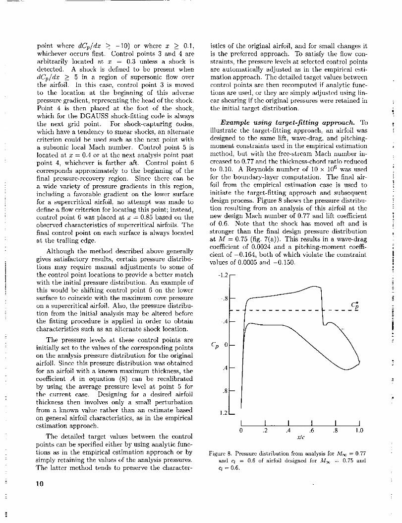
Example using target-fitting approach. To

illustrate the target-fitting approach, an airfoil was

designed to the same lift, wave-drag, and pitching-

moment constraints used in the empirical estimationmethod, but with the free-stream Mach number in-creased to 0.77 and the thickness-chord ratio reduced

to 0.10. A Reynolds numbcr of 10 x 106 was used

for the boundary-layer computation. The final air-foil from the empirical estimation case is used to

initiate the target-fitting approach and subsequent

design process. Figure 8 shows the pressure distribu-

tion resulting from an analysis of this airfoil at thenew design Mach number of 0.77 and lift coefficientof 0.6. Note that the shock has moved aft and is

stronger than the final design pressure distribution

at M = 0.75 (fig. 7(a)). This results in a wave-dragcoefficient of 0.0024 and a pitching-moment coeffi-

cient of -0.164, both of which violate the constraintvalues of 0.0005 and -0.150.

-1.2 --

Cp

-.8

-.4 --

0--

.4 --

.8--

1.2_

I I I I I I0 .2 .4 .6 .8 1.0

x/c

Figure 8. Pressure distribution from analysis for Aloe = 0.77and cl = 0.6 of airfoil designed for /ll_c = 0.75 andcl = 0.6.

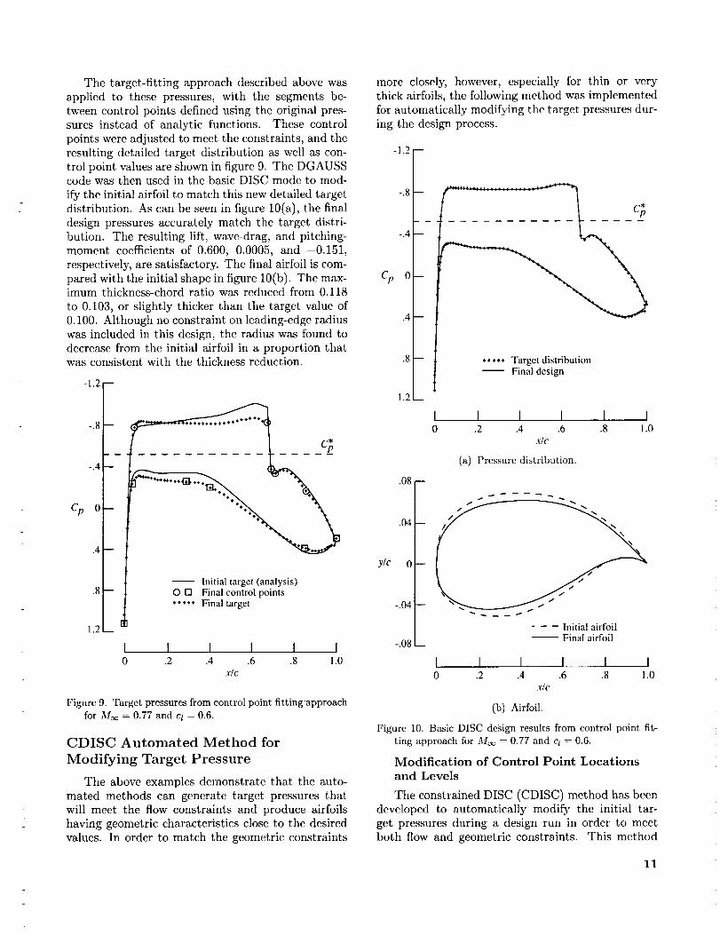
Thetarget-fittingapproachdescribedabovewasappliedto thesepressures,with the segmentsbe-tweencontrolpointsdefinedusingtheoriginalpres-suresinsteadof analyticfunctions. Thesecontrolpointswereadjustedto meettheconstraints,andtheresultingdetailedtargetdistributionaswellascon-trol pointvaluesareshownin figure9. TheDGAUSScodewasthenusedin thebasicDISCmodeto mod-ify theinitial airfoilto matchthisnewdetailedtargetdistribution.Ascanbeseenin figure10(a),thefinaldesignpressuresaccuratelymatchthe targetdistri-bution. Theresultinglift, wave-drag,andpitching-momentcoefficientsof 0.600,0.0005,and -0.151,respectively,aresatisfactory.Thefinalairfoiliscom-paredwith theinitial shapein figure10(b).Themax-imumthickness-chordratiowasreducedfrom0.118to 0.103,or slightlythickerthan thetargetvalueof0.100.Althoughnoconstraintonleading-edgeradiuswasincludedin thisdesign,theradiuswasfoundtodecreasefromtheinitial airfoil in a proportionthatwasconsistentwith thethicknessreduction.

-1.2--

cp

-g --

-.4 --

0--

.4 --

.8 --

1.2_

I0

-- Initial target (analysis)

O [] Final control points

.... * Final target

I I I I I.2 .4 .6 .8 1.0

x/c

Fignlre 9. Target pressures from control point fittingapproachfor Mo_ = 0.7T and q = 0.6.

CDISC Automated Method for

Modifying Target Pressure

The above examples demonstrate that the auto-mated methods can generate target pressures that

will meet the flow constraints and produce airfoils

having geometric characteristics close to the desired

values. In order to match the geometric constraints

more closely, however, especially for thin or verythick airfoils, the following method was implemented

for automatically modifying the target pressures dur-

ing the design process.

-1.2 --

-,8 --

-.4 --

Cp 0-

,4 --

,8 --

1.2_

.08 --

.04 --

y/c 0--

-.04 --

-.08 --

..... Target distribution

Final design

I I I I I I0 .2 .4 .6 .8 1.0

X/C

(a) Pressure distribution.

j f f _

- - - Initial airfoil

-- Final airfoil

I I I I I I0 .2 .4 .6 .8 1.0

xlc

(b) Airfoil.

Figure 10. Basic DISC design results from control point fit-ting approach for -_Ioc = 0.77 and q = 0.6.

Modification of Control Point Locations

and Levels

The constrained DISC (CDISC) method has been

developed to automatically modify the initial tar-

get pressures during a design run in order to meetboth flow and geometric constraints. This method

11

for targetpressuremodificationissimilarto theem-pirical estimationapproachfor targetgenerationinthat it utilizesspecifiedpressure-geometryrelation-ships:The maindifferenceis that whenmodifyingthetargetpressures,perturbationformsof theequa-tionsareusedinsteadof the absoluterelationshipsdevelopedfor target generationsincethe geomet-ric parameterscorrespondingto the currenttargetpressuresareknown.Forexample,therelationshipbetweenmaximumairfoil thicknessandthe averagepressurelevelat controlpoint5giveninequation(8)becomes

A(At/c) (16)

acp-

where At/c is the difference between the desired andcurrent airfoil maximum thickness-chord ratios and

ACp is the required change to the pressure coefficientof control point 5 on each surface. Although a di-

rect differentiation of equation (8) yields A = -3.3,a value of -6.0 has been found to result in faster

convergence. Equation (16) is generally valid exceptin the immediate vicinity of the leading and trailing

edges. In addition to controlling the global parame-

ter of maximum thickness, equation (16) is used toenforce a minimum local thickness constraint at the

average chord location for control point 6.

The leading-edge radius of the airfoil is altered

by changing the chordwise locations rather than thepressure levels of control point 2. A forward shift of

the points will result in a blunter airfoil, whereas alocation farther aft will reduce the nose radius. The

required movement for the points is estimated from

the equation

ax = 0.0002 (17)

where Cle is the magnitude of the leading-edge cur-

vature (the reciprocal of the radius) and ACle is thedifference between the desired and current values.

After the new control point locations for meet-

ing the thickness and radius constraints have beendetermined, the detailed target distributions must

be adjusted accordingly. If the pressures betweencontrol points have been defined using analytic func-

tions, the new levels are simply recomputed by using

the new end points for the same functions. If the

target-fitting approach is used, the new levels asso-ciated with the thickness changes are obtained by

using a linear shearing as in the target generation.For the leading-edge-radius adjustment, the detailed

pressures are modified in a two-step process. First,

the x's for the points between control points 1 and 3

are linearly incremented, based on the change at con-

trol point 2, while the pressure level associated with

each point is held constant. Since the current imple-

mentation of the DISC design method expects the

target pressures to be specified at the grid point lo-cations, a second step is required in which the pres-

sure coefficients at the original streamwise locations

are interpolated from the new distribution. Afterall these geometry-related modifications have been

made, the pressure levels at control points 2, 3, 4,

and 6 are adjusted to satisfy the flow constraints.

Figure 11 illustrates how the CDISC method for

modifying the target pressures has been incorporated

into the basic DISC design method. After everythird call to the DISC design module, the geomet-

ric parameters for the curr_ent airfoil are determinedand passed to the target modification module where

the appropriate adjustments are made to the control

points and detailed target pressures. The new de-

tailed target is then passed back to the design mod-ule for use in the next design update. This approach

allows the flow solution, airfoil design, and target

specification to converge in parallel, thus reducing

the computer resources required.

Initial geometry andflow conditions

y_

I Aerodynamicanalysis module

Pressure distributionfor current geometry

Initial target L_

Design [4]module I-

IlI Compute geometry

parameters. [Modify target pressures I

Figure 11. Flowchart of CDISC design method.

Example Using CDISC TargetModification Approach

As an illustration of this approach, the CDISC

method was applied to the target from the target-

fitting design example (see fig. 10) in an effort tomatch the geometric constraints more closely. As the

design proceeds, this distribution is adjusted based

on the current geometric parameters, and it even-

tually arrives at the final target shown in figure 12.The final design pressures match this target very well

(fig. 13(a)) and all the flow constraints are met. The

initial and final airfoils from the design are compared

in figure 13(b). The maximum airfoil thickness-chordratio was reduced from 0.103 to the desired value

12

of 0.100,andtheleading-edgeradiuswasincreasedfrom0.0073to 0.0107,closeto theconstraintvalueof 0.0110.A third geometricconstraintwasimposedto maintainthe thicknessof the initial airfoilat thelocationof controlpoint 6, that is, x = 0.85. Thefinal thickness at this location was within +0.0004c

of the specified value. Since relatively minor changes

to the initial target distribution were required, the

CDISC design process required the same amount of

computer time as the basic DISC design in the target-

fitting example (approximately 143 cpu seconds on aCray Y-MP computer).

-!.2 --

cp

-.8 m

-.4 m

0--

.4 --

.8 --

1.2m

I0

- - - Initial targetModified target

I I I I I.2 .4 .6 .8 1.0

x/c

Figure 12. Target pressures from CDISC design case forM_c = 0.77 and ct = 0.6.

Glove Constraint Option and Example

An additional geometric constraint implementedin the CDISC approach is the "glove" option. In this

option, the design surface geometry is required to re-main between inner and outer bounding surfaces over

a specified chordwise region. This capability would

be used, for example, in the design of a wing glove

for flight research where the new geometry must lieoutside the existing wing shape or spar box, or for

developing an efficient external shape that encloses

an internal aircraft component such as an antenna.

Although this set of constraints could be addressed

directly by restricting the aerodynamic surface coor-dinates from penetrating the bounding surfaces, this

approach would allow little, if any, control over the

resulting flow characteristics. Therefore, an indirect

approach involving target pressure alteration was

developed.

The detailed target pressures are modified using

a pressure-geometry relationship similar to that of

equation (16), except that a desired change in surfaceordinate is used instead of a change in thickness, and

the coefficient A changes sign for the lower surface of

an airfoil. Although strictly valid only for subsonicflow, this relationship has also been used successfully

in mildly supercritical flow.

-1.2 -

Cp 0

..... Target distributionFinal design

I I I I 1•2 .4 .6 .8 1.0

X/C

(a) Pressure distribution.

.08 m

.04--

y/c 0

-.04

-.08

- - - Initial airfoilFinal airfoil

I I I I I I0 .2 .4 .6 .8 1.0

x/c

(b) Airfoil.

Figure 13. CDISC design results for M_ = 0.77 and cl = 0.6.

13

Threeapproachesfor alteringthedetailedtargetpressuredistributionareinvestigated.Thefirst ap-proachsimplychecksfor penetrationof the bound-ing surfaceat eachpoint in the constraint,regionandadjuststhepressurecoefficientlocallybasedonthe magnitudeof the penetration.An alternativeapproachis to determinethe maximumpenetrat{ondistanceandadjustall thetargetpressuresovertheconstraintregionby a constantincrementbasedonthat distance.Thisapproachisusefulforcaseswheremaintaininga specifiedgradientin the targetpres-suresis desirable,as in laminarflowdesigns.Thethird approachis a modificationof theconstantin-crementprocedurethat usesalinearlyvaryingincre-ment.With thisapproach,oneendofthesegmentofthepressuredistributionovertheconstraintregionisfixedandtherestof thesegmentis linearlyshearedto meetthe no-penetrationcriteria. Thisapproachcanyield themaximumfavorablegradientthat sat-isfiesboth thegeometricconstraintanda wave-dragconstraint.

Toillustratetheseapproaches,a naturallaminarflow (NLF) glovewasdesignedfor anairfoil. Thiseaserepresentsanautomatedapproachto theVari-ableSweepTransitionFlight Experiment(VSTFE)designexerciseusinganF-14reportedbyWaggoner,Campbell,andPhillips (1985),whichrequirednu-merousmanualmodificationsto thetargetpressuresaswellasairfoilgeometriesto developgloveshapesthat metboththeflowandgeometricconstraints.Atthewingstationselectedfor thiscase,theglovebe-gan0.02caheadof the leadingedgeof thebaselineairfoilandextendedto x/c = 0.58 on the upper sur-

face and to x/c = 0.30 on the lower surface. Since theactual glove on the upper surface terminated in an

aft-facing step, a computational fairing was included

by extending the upper surface design region to x/c-- 0.70.

In addition to tile chordwise extent of the de-

sign region, geometric constraints were imposed by

the existing airfoil shape and allowable glove thick-

nesses. These constraints were used to develop innerand outer bounding surfaces for constrained design.

Tile baseline airfoil coordinates comprised the inner

bounding surface except on the upper surface ahead

of x/c = 0.50 where 0.0065c was added to the ordi-nates to allow for installation of pressure measure-

ment tubes. The original design constraints required

that the glove thickness at x/c = 0.58 on the upper

surface be no more than 0.01c to reduce any adverse

effects caused by the aft-facing step. A more conser-

vative maximum glove thickness of 0.005c was used

from x/c = 0.58 to 0.70 in order to demonstrate the

outer bounding surface capability.

14

The main flow constraint for this case was to avoid

an adverse pressure gradient over the front half of the

upper surface so that natural laminar flow could be

maintained in this region. This constraint was to be

met at the design lift coefficient with no shock de-velopment. A target pressure distribution was gen,

crated by first analyzing the initial airfoil at the two-

dimensional design conditions of Moc = 0.65 and

cI = 0.6. This distribution was then modified on

the upper surface by specifying a quartie distribu-

tion of pressure coefficients between the leading edgeand x/c = 0.01, followed by a pressure coefficient

gradient of -0.05 aft to x/c = 0.50. (See fig. 14.)

This favorable gradient was deliberately chosen to

represent a design case that was more difficult than

the neutral gradient cases reported by Waggoner,

Campbell, and Phillips (1985). The initial pressurelevels in this region were adjusted to match the orig-inal lift coefficient of 0.6.

-1.2

-.8

-.4

Cp 0

.4

.8

1.2

I0

-- Analysis of baseline airfoil

..... Initial glove target

I I I I I.2 .4 .6 .8 1.0

x/c

Figure 14. Pressure distribution of initial glove target forMo_ = 0.65. "_

The initial airfoil for the design was developed

by linearly shearing the coordinates of the baseline

airfoil in the design region on each surface to extend

forward to the leading edge of the glove. This airfoilwas then translated and nondimensionalized so that

the leading and trailing edges were again at x/c =

0 and 1.0, respectively. Finally, these coordinateswere smoothed to blend the stretched regions into

the original airfoil.

-I.2--

-.8 i

-.4 --

Cp 0-

.4 --

.8 --

t.2_

.08 --

.04 --

y/c 0 --

-.04

-.08 --

..... Target distributionFinal design

I I I I l j0 .2 .4 .6 .8 1.0

X/C

(a) Pressure distribution.

I I0 .2

- - Initial airfoil-- Final airfoil,-rvm Constraint surfaces

I I I I.4 .6 .8 1.0

x/c

(b) Airfoil.

Figure 15. Results of basic (unconstrained) DISC design forinitial glove target for M_ = 0.65.

The code was first run in the basic DISC designmode to match the initial target pressure distribu-

tion. As shown in figure 15(a), the final pressures

match the target values fairly well on the lower sur-

face and over the constant gradient portion of the

upper surface. On the upper surface, slight over-shoots of the targets occur at the beginning and end

of the constant gradient region. The steep recoverygradient near midchord has been reduced as a result

of the airfoil smoothing done during the design. A

mismatch between target and design pressures also

occurs at the end of the design region (x/c = 0.70),thus indicating a discontinuity in curvature at this

point. Again, since the actual flight glove would end

at x/c = 0.58, this discrepancy is not significant. "A

comparison of the resulting design geometry with the

bounding surfaces (fig. 15(b)) shows that the innersurface constraint is violated on the upper surfaceover most of the front half of the chord.

The design was therefore repeated by using the

glove constraint option. All three pressure modifi-cation approaches were used in this example. On

the upper surface, the constant gradient method was

used ahead of x/c = 0.50, with smoothing used to

blend the steep leading-edge acceleration into the

mild favorable gradient as the level was adjusted.

Between x/c = 0.50 and 0.70, the linearly varying

increment approach (with the aft end of the target

segment fixed) was used to ensure that the pressuresmatched those for the initial target at the end of

the design region. On the lower surface, the individ-

ual point adjustment technique was used, again with

smoothing employed to fair into the fixed portion of

the target distribution.

-1.2 --

-.4 i

Cp 0-

.4 --

.8 i

1.2--

- - Initial targetModified target

I I I I I I0 .2 .4 .6 .8 1.0

x/c

Figure 16. Target pressures from CDISC glove design forMoc = 0.65.

The modifications made by the design code to the

initial target pressures are shown in figure 16. The in-ner surface constraint drove the level of the constant

gradient section on the upper surface toward more

15

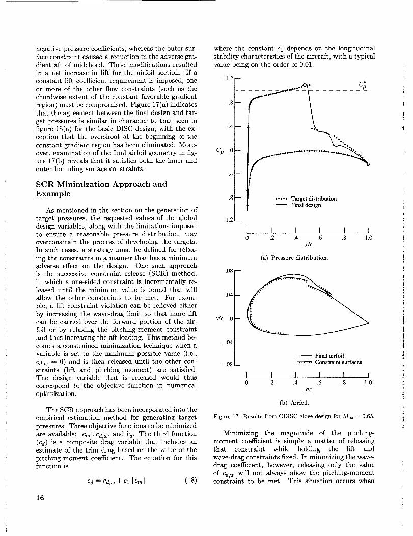
negativepressurecoefficients,whereastheoutersur-faceconstraintcausedareductionin theadversegra-dientaft of midchord.Thesemodificationsresultedin a net increasein lift for the airfoil section,if aconstantlift coefficientrequirementis imposed,oneor moreof the other flowconstraints(suchasthechordwiseextentof the constantfavorablegradientregion)mustbecompromised.Figure17(a)indicatesthat theagreementbetweenthefinaldesignandtar-getpressuresis similarin characterto that seeninfigure15(a)for thebasicDISCdesign,with theex-ceptionthat the overshootat the beginningof theconstantgradientregionhasbeeneliminated.More-over,examinationof thefinalairfoilgeometryin fig-ure17(b)revealsthat it satisfiesboththeinnerandouterboundingsurfaceconstraints.

SCR Minimization Approach and

Example

As mentioned in the section on the generation of

target pressures, the requested values of the global

design variables, along with the limitations imposedto ensure a reasonable pressure distribution, may

overconstrain the process of developing the targets.

In such cases, a strategy must be defined for relax-

ing the constraints in a manner that has a minimumadverse effect on the design. One such approach

is the successive constraint release (SCR) method,

in which a one-sided constraint is incrementally re-leased until the minimum value is found that will

allow the other constraints to be met. For exam-

ple, a lift constraint violation can be relieved eitherby increasing the wave-drag limit so that more lift

can be carried over the forward portion of the air-

foil or by relaxing the pitching-moment constraint

and thus increasing the aft loading. This method be-comes a constrained minimization technique when a

variable is set to the minimum possible value (i.e.,

Cd,w ---- 0) and is then released until the other con-straints (lift and pitching moment) are satisfied.

The design variable that is released would thus

correspond to the objective function in numericaloptimization.

The SCR approach has been incorporated into the

empirical estimation method for generating target

pressures. Three objective functions to be minimized

are available: lCml, Cd,w, and Cd. The third function(Sd) is a composite drag variable that includes anestimate of the trim drag based on the value of the

pitching-moment coefficient. The equation for thisfunction is

Cd = Cd,w + Cl [Crn[ (18)

16

where the constant Cl depends on the longitudinal

stability characteristics of the aircraft, with a typical

value being on the order of 0.01.

cr

y/c

-1.2 --

-.8--

-.4 m

0--

.4--

.8 --

1.2--

÷¢

..... Target distribution-- Final design

[ I I I I I0 .2 .4 .6 .8 1.0

x/c

(a) Pressure distribution.

.08 --

-.04

-.08

.04--

0--

-- Final airfoilConstraint surfaces

I I I I I I0 .2 .4 .6 .8 1.0

X/C

(b) Airfoil.

Figure 17. Results from CDISC glove design for Mc¢ = 0.65.

Minimizing the magnitude of the pitching-

moment coefficient is simply a matter of releasing

that constraint while holding the lift and

wave-drag constraints fixed. In minimizing the wave-

drag coefficient, however, releasing only the value

of Cd,w will not always allow the pitching-momentconstraint to be met. This situation occurs when

the shocklocation(controlpoint 3) is at or aft ofx _ 0.5 - (X2)uppe r. For this shock location, the in-crease in lift between points 2 and 3 on the upper sur-

face due to releasing the wave-drag constraint is bal-

anced about the moment reference center (x = 0.25),

with the result that no change in pitching momentoccurs. For these cases, the pitching-moment con-

straint must also be relaxed. In minimizing the third

objective function (cd), the wave drag and pitching

moment are initially set to 0, and then the pitching-

moment coefficient is released until the remainingconstraints are satisfied. The wave-drag coefficient is

then incremented and the pitching moment is again

minimized. This process continues as long as the re-

sulting values of _d are decreasing. This termina-tion criterion assumes that the first minimum en-

countered is an absolute minimum. This criterion

has also been altered to explore a broader matrix of

wave drag and pitching moment to ensure that the

true minimum is found, but experience thus far has

indicated that the original assumption is valid.

-2.4 --

-2.0

-1.6

-1.2

-.8

-.4

.4

.8

1.2

m

I I I0 .2 .4

x/c

I.6

I,8

I1.0

Figure 18. Analysis of NACA 0025 airfoil at Mc_ = 0.6 andcl -= 0.6.

The procedures described above minimize the ob-

jective functions for a given shock location. In order

to provide a more general minimization capability, an

option has been included for automatically determin-

ing the minimum value of the functions over a rangeof shock locations. A default range is defined as 0.1c

forward and aft of the estimated shock location given

by equation (10).

To illustrate the constrained minimization capa-

bility, a 25-percent-thick airfoil was designed at Moo

= 0.6 and c I = 0.6 with the objective of minimizing

Cd. (For this case, c 1 was arbitrarily set to 0.01.)The airfoil thickness was selected as being repre-

sentative of an advanced-technology, high-altitude,

long-endurance aircraft (Hall 1990), and therefore it

should provide a good indication of the generalityof the empirical relationships used to generate the

initial target pressures. Although wave drag would

not ordinarily be a concern at this design Mach num-

ber, the large thickness-chord ratio and moderate lift

coefficient could easily result in transonic flow. Forexample, analysis of an NACA 0025 airfoil at the de-

sign Mach number and lift coefficient shows that a

strong shock is present near x/c = 0.3 (fig. 18), thus

resulting in a wave-drag coefficient of 0.0057.

.0005 -

.0004

.0003

.0002

.0001-

Default shock /

_-- Default search range _

I I I i I , I.2 .3 .4 .5

(x/c)shock

Figure 19. Minimum values of composite drag function forvarious shock locations for a 25-percent-thick airfoil atMo_ = 0.6 and et = 0.6.

The SCR method was used to generate the initial

target pressures for this case. Figure 19 shows thevalues of Cd obtained by this minimization process

for shock locations ranging from x/c = 0.2 to 0.5.

The minimum value for Cd of about 0.0001 was found

to occur near x/c = 0.3. The curve has a veryshallow character, however, so that the shock can be

placed anywhere between x/c = 0.25 and 0.40 andstill be within +0.0001 of the minimum. Note that

17

thedefaultshocklocationof x/c = 0.36 determinedfrom equation (10) is within this region, and that this

region would be included ill the default shock-search

range of x/c = 0.26 to 0.46.

-1.2

-2.0 --

-1.6 --

-.8 --

0--

.4 --

.8 --

1.2_

Io

Cp -.4

Initial targetModified target

I I I I I.2 .4 .6 .8 1.0

x/c

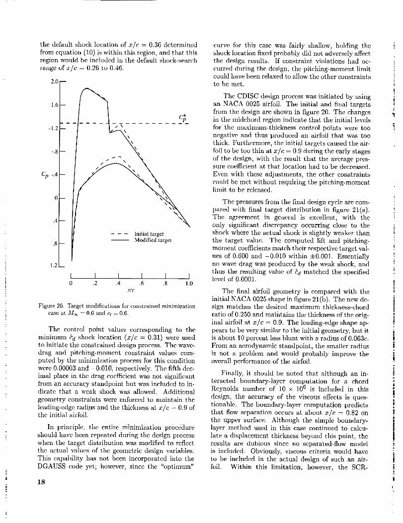
Figure 20. Target modifications for constrained minimization

case at M_c = 0.6 and ct = 0.6.

The control point values corresponding to the

minimum Cd shock location (x/c = 0.31) were usedto initiate the constrained design process. The wave-

drag and pitching-moment constraint values com-puted by the minimization process for this condition

were 0.00003 and -0.010, respectively. The fifth dec-

imal place in the drag coefficient was not significant

from an accuracy standpoint but was included to in-dicate that a weak shock was allowed. Additional

geometry constraints were enforced to maintain the

leading-edge radius and the thickness at x/c = 0.9 ofthe initial airfoil.

In principle, the entire mlnimization procedureshould have been repeated during the design process

when the target distribution was modified to reflect

the actual values of the geometric design variables.

This capability has not been incorporated into the

DGAUSS code yet; however, since the "optimum"

18

curve for this case was fairly shallow, holding the

shock location fixed probably did not adversely affectthe design results. If constraint violations had oc-

curred during the design, the pitching-moment limitcould have been relaxed to allow the other constraintsto be met.

The CDISC design process was initiated by using

an NACA 0025 airfoil. The initial and final targets

from the design are shown in figure 20. The changesin the midchord region indicate that the initial levels

for the maximum-thickness control points were toonegative and thus produced an airfoil that was too

thick. Furthermore, the initial targets caused the air-

foil to be too thin at x/c = 0.9 during the early stagesof the design, with the result that the average pres-sure coefficient at that location had to be decreased.

Even with these adjustments, the other constraints

could be met without requiring the pitching-momentlimit to be released.

The pressures from the final design cycle are com-pared with final target distribution in figure 21(a).

The agreement in general is excellent, with the

only significant discrepancy occurring close to theshock where the actual shock is slightly weaker than

the target value. The computed lift and pitching-

moment coefficients match their respective target val-

ues of 0.600 and -0.010 within ±0.001. Essentiallyno wave drag was produced by the weak shock, and

thus the resulting value of Cd matched the specifiedlevel of 0.0001.

The final airfoil geometry is compared with the

initial NACA 0025 shape in figure 21(b). The new de-sign matches the desired maximum thickness-chord

ratio of 0.250 and maintains the thickness of the orig-

inal airfoil at x/c = 0.9. The leading-edge shape ap-

pears to be very similar to the initial geometry, but itis about 10 percent less blunt with a radius of 0.063c.

From an aerodynamic standpoint, the smaller radius

is not a problem and would probably improve theoverall performance of the airfoil.

Finally, it should be noted that although an in-

teracted boundary-layer computation for a chordReynolds number of l0 × 106 is included in this

design, the accuracy of the viscous effects is ques-

tionable. The boundary-layer computation predicts

that flow separation occurs at about x/c = 0.82 onthe upper surface. Although the simple boundary-layer method used in this case continued to calcu-

late a displacement thickness beyond this point, theresults are dubious since no separated-flow model

is included. Obviously, viscous criteria would have

to be included in the actual design of such an air-

foil. Within this limitation, however, the SCR-

constrainedminimizationapproachdid succeedinproducinga very reasonableairfoil geometrythat,in general,met the constraintsandobjectivesandrequiredonlyglobaldesignparametersasinput.

-2.0--

-1.6-

-1.2-

-.8 --

Cp -.4 --

0--

,4 --

.8 --

1.2__

I0

.... * Target distributionFinal design

I I I I I.2 .4 .6 .8 1.0

x/c

(a) Pressure distribution.

.16 --

-.08

-.16

.08 --

yh" 0 --

- - Initial airfoil-- Final airfoil

I I I I I I0 .2 .4 .6 .8 1.0

x/c

(b) Airfoil.

Figure 21. CDISC design results for constrained minimizationease at _,I_ = 0.6 and ct = 0.6.

Concluding Remarks

An approach has been developed for incorporat-

ing flow and geometric constraints into the basicDirect Iterative Surface Curvature (DISC) design

method. In this approach, an initial target pres-

sure distribution was developed using a set of control

points. The chordwise locations and pressure levels

of these points were initially estimated either from

empirical relationships and observed characteristics

of pressure distributions for a given class of airfoils or

by fitting the points to an existing pressure distribu-tion. These values were then automatically adjusted

during the design process to satisfy the flow and geo-metric constraints. The constraint options currently

available include flow parameters such as lift, wave

drag, and pitching moment, and also geometric pa-rameters such as maximum thickness, local thickness,

and leading-edge radius. This approach has also bccnextended to include the successive constraint release

(SCR) approach to constrained minimization.

Test cases were included to illustrate both the em-

pirical estimation and the control point fitting ap-proaches to target pressure generation. Basic DISC

design results for each approach indicated that the

flow parameters for the final design met the require-

ments and that the geometric parameters were fairlyclose to the desired values. Thus, either method

could be used to generate a good initial targetdistribution.

The constrained DISC (CDISC) method which

adjusts the target pressures during the design pro-cess was then applied to tile control point fitting ap-

proach listed above. In this example, the constraineddesign procedurc produced an airfoil that accurately

matched the desired geometric values while main-

taining good agreement with the flow constraints.

Since relatively minor changes to the initial targetdistribution were required and a simultaneous flow,

design, and target convergence approach was used,

the CDISC design process required about the sameamount of computer time as the basic DISC design.

An example of a second constrained design was

given to illustrate a "glove" constraint capability.The results showed that the specified favorable pres-

sure gradient over the front half of the upper surfaceof the airfoil was maintained and that the inner and

outer bounding surface constraints were not violated.

The final example of a constrained design demon-strated the SCR minimization approach applied to

the design of a thick airfoil. The SCR approach was

used in conjunction with the empirical estinmtion ap-proach to define an initial target distribution with

a shock location, wave drag, and pitching moment

19

that yielded the minimum value of a composite drag

objective function. The constrained dcsign process

did not make large changes to the target prcssures,

thus indicating that the empirical relationships used

to generate the initial target may be used for a wide

range of airfoil thickncsses. The final design met all

the constraintsl

The CDISC design method in combination with

the SCR minimization approach thus offers an effi-

cient and accurate approach to aerodynamic design.

Since the target pressure generation and modifica-

tion are automated and require only global param-

eters as input, the amount of manual intervention

needed is greatly reduced. Also, the simultaneous

convergence of the flow field, design geometry, and

target pressures allows the constrained designs to be

obtained very efficiently. This efficiency, along with

the use of global design variables, makes the CDISC

approach an attractive alternative to numerical opti-

mization. Finally, although this report demonstrates

only tile capabilities for airfoil design, the concepts

are amenable to three-dimensional design problems.

NASA Langley Research Center

Hampton, VA 23681-0001

September 30, 1992

References

Anon. 1990a: Computational Methods for Aerodynamic De-

.sign (Inverse) and Optimization. AGARD-CP-463.

Anon. 1990b: Special Course on Inverse Methods for Air-

foil Design for Aeronautical and Turbomachinery Appli-cations. AGARDiR-780.

Bell, R. A.; and Cedar, R. D. 1991: An Inverse Method

for the Aerodynamic Design of Three-Dimensional Air-

craft Engine Nacelles. Proceedings Third International

Conference on Inverse Design Concepts and Optimiza-

tion in Engineering Sciences ICIDES-HI, George S.

Dulikravich, ed., Pennsylvania State Univ., pp. ,105 417.

Campbell, Richard L.; and Snfith, Leigh A. 1987a: Designof Transonic Airfoils and Wings Using a Hybrid Design

Algorithm. SAE Tech. Paper Set. 871756.

Campbell, Richard L.; and Smith, Leigh A. 1987b: A Hy-

brid Algorithm for _ans0n_c Airfoil and Wing Design. A

Collection of Technical Papers AIAA 5th Applied Aero-

dynamics Conference, American Inst. of Aeronautics and

Astronautics, pp. 527 538. (Available a.s AIAA-87-2552.)

Dulikravich, George S. 1990: Aerodynamic Shape Design.

Special Course on Inverse Methods for AiTfoil Design for

Aeronautical and Turbomaehinery Applications, AGARD-

R-780, pp. 1-1 1-10.

Giles, Michael; and Drela, Mark 1986: A Two-

Dimensional Transonic Aerodynamic Design Method. A

Collection of Technical Papers, AIAA _th Applied Aero-

dynamics Conference, American Inst. of Aeronautics and

Astronautics, pp. 197 204. (Available as AIAA-86-1793.)

Hall, Douglas R. 1990: Thick Airfoil Designs for a Hale

Vehicle. A Collection of Technical Papers, Part 1

AIAA 8th Applied Aerodynamics Conference, pp. 323

331. (Available as AIAA-90-3036-CP.)

Hartwich, Peter-M. 1990: Fresh Look at Floating Shock

Fitting. AIAA-90-0108.

Hicks, Raymond M.; Murman, Earll M.; and Vanderplaats,

Garret N. 1974: An Assessment of Airfoil Design by

Numerical Optimization. NASA TM X-3092.

Lin, W. F.; Chen, A. W.; and Tinoco, E. N. 1990: 3D Tran-

sonic Nacelle and Winglet Design. A Collection of Tech-

nical Papers, Part 2 AIAA 8th Applied Aerodynamics

Conference, pp. 582 591. (Available as AIAA-90-3064.)

Lock, R. C. 1985: Prediction of the Drag of Wings at Sub-

sonic Speeds by Viscous/Inviscid Interaction Techniques.

Aircraft Drag Prediction and Reduction, AGARD-R-723,

pp. I0-1 10-71.

Malone, J. B.; Narramore, J. C.; and Sankar, L. N. 1990: An

Efficient Airfoil Design Method Using the Navier-Stokcs

Equations. Computational Method_ for Aerodynamic De-

sign (Inverse) and Optimization, AGARD-CP-463, pp. 5-1 5-18.

Nash, J. F.; and Macdonald, A. G. J. I967: The Calculation

of Momentum Thickness in a Turbulent BoundaT'y Layer

at Mach Numbers up to Unity. C.P. No. 963, British

Aeronautical Research Council.

Oswatitsch, Klaus (English version by Gustav Kuerti) 1956:

Gas" Dynamics. Volume I of Applied Mathematics and

Mechanics, Academic Press, Inc., pp. 447 497.

Smith, Leigh Ann; and Campbell, Richard L. 1991: A Method

for the Design of Transonic Flexible Wings. NASA TP-

3045.

Sobieczky, H.; Yu, N. J.; Fung, K.-Y.; and Seebass, A. R.

1979: New Method for Designing Shock-Free Transonic

Configurations. AIAA J., vol. 17, no. 7, pp. 722-729.

Squire, H. B.; and Young, A. D. 1938: The Calculation of

the Profile Drag of Aerofoils. R. & M. No. 1838, BritishAeronautical Research Council.

Stratford, B. S.; and Beavers, G. S. 1961: The Calculation of

the Compressible Turbulent Boundary Layer in an Arbi-

trary Pressure Gradient A Correlation of Certain Pre-

vious Methods. R. & M. No. 3207, British Aeronautical

Research Council.

Van den Dam, R. F.; Van Egmond, J. A.; and Slooff, J. W.

1990: Optimization of Target Pressure Distributions. Spe-

cial Course on Inverse Methods for Airfoil Design for

Aeronautical and Turbomachinery Applications, AGARD-

R-780, pp. 3-1 3-13.

20

VanEgmond,J.A.1990:NumericalOptimizationofTargetPressureDistributionsforSubsonicandTransonicAirfoilDesign.Computational Methods for Aerodynamic Design

(Inverse) and Optimization, AGARD-CP-463, pp. 17-1-

17-11.

Volpe, G.; and Melnik, R. E. 1985: A Method for Designing

Closed Airfoils for Arbitrary Supercritical Speed Distri-

butions. AIAA-85-5023.

Waggoner, Edgar G.; Campbell, Richard L.; and Phillips,

Pamela S. 1985: Computational Wing Design in Support

of an NLF Variable Sweep Transition Flight Experiment.

AIAA-85-4074.

Wie, Y. S.; Collier, F. S., Jr.; and Wagner, R. D. 1991: Ap-

plication of Laminar Flow Control to High-Bypass-Ratio

Turbofan Engine Nacelles. SAE Tech. Paper Ser. 912114.

21

Form ApprovedREPORT DOCUMENTATION PAGEOMB No 0704 0188

Public reporting burden for this corlection of information is estimated to average I hour per response, including the time for reviewing instructions, searching existing data sources.gathering and maintaining the data needed, and completing and reviewing the collection of information Send comments regarding this burden estimate or any other aspect of thiscollection of information, including suggestions for reducing this burden, to Washington Headquarters Services, Directorate for Information Operations and Reports, 1215 JeffersonDavis Highway, Suite 1204, Arlington, VA 22202 4302, and to the Office of Management and Budget, Paperwork Reduction Project (0704-0t88), Washington, DC 20503

1. AGENCY USE ONLY(Leave blank) 2. REPORT DATE 3. REPORT TYPE AND DATES COVERED

November 1992 Technical Paper

4. TITLE AND SUBTITLE 5. FUNDING NUMBERS

An Approach to Constrained Aerodynamic Design WithApplication to Airfoils WU 505-59-10-03

6. AUTHOR(S)

Richard L. Campbell

7. PERFORMING ORGANIZATION NAME(S) AND AOORESS(ES)

NASA Langley Research Center

Hampton, VA 23681-0001

9. SPONSORING/MONITORING AGENCY NAME(S) AND ADDRESS(ES)

National Aeronautics and Space Administration

Washington, DC 20546-0001

8. PERFORMING ORGANIZATION

REPORT NUMBER

L-17108

10. SPONSORING/MONITORING

AGENCY REPORT NUMBER

NASA TP-3260

11. SUPPLEMENTARY NOTES

12a. DISTRIBUTION/AVAILABILITY STATEMENT

Unclassified Unlimited

Subject. Category 02

12b. DISTRIBUTION CODE

13. ABSTRACT (Maximum 200 words)

An approach has been developed for incorporating flow and geometric constraints into the Direct Iterative

Surface Curvature (DISC) design method. In this approach, an initial target pressure distribution is developedusing a set of control points. The chordwise locations and pressure levels of these points are initially estinmted

either from empirical relationships and observed characteristics of pressure distributions for a given class of

airfoils or by fitting the points to an existing pressure distribution. These values are then automatically adjustedduring the design process to satisfy the flow and geometric constraints. The flow constraints currently available

are lift, wave drag, pitching moment, pressure gradient, and local pressure levels. The geometric constraint

options include maximum thickness, local thickness, leading-edge radius, and a "glove" constraint involvinginner and outer bounding surfaces. This design method has also been extended to include the successive

constraint release (SCR) approach to constrained minimization.

14. SUBJECT TERMS

Airfoil design; Design method

17. SECURITY CLASSIFICATION

OF REPORT

Unclassified

'NSN 7540-01-280-5500

18. SECURITY CLASSIFICATIOI_

OF THIS PAGE

Unclassified

19. SECURITY CLASSIFICATION

OF ABSTRACT

15. NUMBER OF PAGES

22

16. PRICE CODE

A03

20. LIMITATION

OF ABSTRACT

Standard Form 298(Rev. 2-89)Prescribed by ANSI Std Z39-18298-102

NASA-Langley, 1992

JZ

L

i

J

z