An Anthropometric History

of the Postbellum US,

1847-1894

Inaugural-Dissertation

zur Erlangung des Grades

Doctor oeconomiae publicae (Dr. oec. publ.)

an der Ludwig-Maximilians-Universität München

2010

vorgelegt von

Matthias Zehetmayer

Referent: Prof. John Komlos, Ph.D. Korreferent: Prof. Dr. Ekkehart Schlicht

Promotionsabschlussberatung: 17. November 2010

Mündliche Prüfung am 2. November 2010

Berichterstatter:

Prof. John Komlos, PhD (vertreten durch Prof. Ray Rees, PhD)

Prof. Dr. Ekkehart Schlicht

Prof. Dr. Joachim Winter

i

ACKNOWLEDGEMENTS

I am extremely grateful for the advice and support of Prof. John Komlos, for being such a

dedicated and enthusiastic mentor, and for awakening my interest in economic and

anthropometric history.

I thank Takeshi Amemiya, Olga Arnold, Jörg Baten, Ariane Breitfelder, Ted and Diane

Bright, Francesco Cinnirella, Timothy Cuff, Özgür Ertac, Michael Haines, Martin Hiermeyer,

Daniel Koch, Michal Masika, Ruth and Steve Nash, Linda Rousova, Michael Specht, Martin

Spindler, Marco Sunder, Marianne Wanamaker, Martin Watzinger, Tom Weiss, Andreas

Widenhorn, Gordon Winder, Dong Woo Yoo, Michael Zabel, and Barbara and Simon

Zehetmayer for helpful comments and conversations.

I would like to thank Prof. Ray Rees, Prof. Ekkehart Schlicht, and Prof. Joachim Winter for

agreeing to be on my doctoral committee.

I am also grateful to the seminar participants at the Economic History Association’s 2009

meeting and the faculty research seminar participants at the University of Munich for valuable

comments and suggestions. All remaining errors are solely mine.

I am very grateful for the support and encouragement of my parents who have made all this

possible.

ii

TABLE OF CONTENTS

Introduction 1

References 7

1. The Postbellum Continuation of the Antebellum Puzzle:

Stature in the US, 1847 - 1894 9

1.1 Introduction 10

1.1.1 Historical Background 10

1.2 Data and Methodology 13

1.3 Results 20

1.3.1 Time Trends in Height 20

1.3.2 County and State Level Determinants of Height 32

1.4 Conclusion 41

References 44

2. Decomposing the Urban American Height Penalty, 1847-1894 48

2.1 Introduction 49

2.2 Data and Methodology 50

2.3 Results 54

2.4 Conclusion 68

References 71

3. Who is Your Daddy and What Does He Do?

Stature and Family Background in the US, 1847-1880 75

3.1 Introduction 76

3.2 Data and Methodology 77

3.3 Linkage Process 81

iii

3.4 Intergenerational Occupational Mobility 84

3.5 Re-estimating the Occupational Height Premiums 88

3.6 Family-Level Correlates of Height 92

3.7 Conclusion 96

References 98

1

Introduction

Stature is an important measure of the standard of living, supplementing as it does other, more

conventional economic measurements, such as Gross Domestic Product (GDP) and personal

income. It is an invaluable resource when it comes to times and places in which such

measurements cannot be made because the data are either unavailable or unreliable. In

contrast, height data from more or less distant times and places are plentiful, waiting to be

gleaned from documents featuring vital statistics on military recruits, students, convicts, oath

takers, passport applicants, runaway slaves, and even skeletal remains (Steckel, 1995).

Height is determined by a mixture of genetic and environmental factors - about 80

and 20%, respectively (Silventoinen, 2003) - but the genetic component’s preponderance

disappears when average heights of (homogeneous) populations are analyzed (Steckel, 1995).

Height summarizes an individual’s history of net nutrition. Since physical labor as well as ill

health take their tolls on the body’s energy, and the residual energy is used for growth, not

only nutritional intake but also energy expenditure matters (Fogel, 1994; Steckel, 1995).

Macronutrients and micronutrients that have a direct impact on stature include protein,

calcium, vitamin D, and zinc (Waterlow, 1994). Whenever a diet is deficient in calories in

general and in these nutrients in particular, an individual’s growth rate declines. However, if

provided with adequate net nutrition following periods of deprivation the human body is

capable of catch-up growth, and the normal growth period can even be extended by several

years. However, if deprivation prevails then stunting results (Waterlow, 1994; Steckel, 1995).

The most severe consequences of short stature are an increase in the risk of chronic diseases

and a decrease in life expectancy (Waaler, 1984; Fogel, 1994). Since height has an upper limit

and nutrient intake produces diminishing returns, stature is an excellent measure of inequality

as well (Steckel, 1995; Komlos, 2009).

2

Human height has been studied since the 18th-century, but it is only in the past 30

years that, thanks to research in the field of anthropometric history its status as an accurate

indicator of the biological standard of living has been established (Steckel, 1995; Steckel,

2009; Komlos, 2009). Between the late 1970s and 1994 papers dealing with human height

appeared at the rate of about five a year, most of the authors approaching the issue from the

vantage point of economic history or development economics; five were published in the four

most highly rated economics journals. Between 1995 and 2008 the number increased more

than fourfold, to 23.3 per year, among them 13 in those four journals (Steckel, 2009). Such a

dramatic increase clearly indicates that the study of stature is an increasingly significant

tributary to mainstream economics.

For economic historians, interested as they are in the economic forces that affect

stature, the United States during the second half of the 19th-century - with the Civil War

(1861-65) as the pivot of an extended period of exceptional economic growth, urbanization,

and market integration - is a particularly fertile field of research. During the period under

consideration here (1847-94) GDP per capita grew 105% and industrial production grew

600% despite the war (Davis, 2004; Johnston and Williamson, 2008). A national economy

emerged as railroad and telegraph networks reduced transportation and communication costs

(Rosenbloom, 1990). Produce, lumber, and coal could now be shipped long distances, a

development that facilitated regional specialization and market integration (James, 1983). The

composition of the labor force changed from nearly 60% agricultural workers in 1850 to

fewer than 40% in 1899 (Lewis, 1979; Weiss, 1992). Farmers in the North and especially in

the Midwest had already begun to shift from self-sufficiency to commercial agriculture,

marketing their surplus (Atack and Bateman, 1984). There was also a shift from home

manufacturing and agriculture to factory production, which, with its crowded and unsanitary

working conditions, facilitated the spread of diseases (Costa and Steckel, 1997). Over the

3

course of the 19th-century American cities grew dramatically, their share of the nation’s total

population increasing from about 6 to 40% (Haines, 2001), but public sanitation, water, and

sewage systems were rudimentary throughout much of the period (Preston and Haines, 1991).

It is therefore not surprising that urban death rates were 1.4 times that of rural ones (Condran

and Crimmins-Gardner, 1980; Haines, 2001). From the 1820s to the 1850s urban inequality,

as measured by Williamson’s (1975, 1976) urban inequality index of pay differentials by skill,

grew by over 60%; it then declined for about a decade, recovering only after the Civil War.

It is not surprising that such an eventful century has prompted a number of noteworthy

discoveries, chiefly that of the Antebellum Puzzle (Margo and Steckel, 1983; Komlos, 1987):

a pattern of declining heights despite rising per capita income, indicating that the biological

standard of living was not in conformity with the conventional welfare indicators in the first

half of the 19th-century - despite an annual 1.4% increase in per capita output between 1830

and 1860 (Weiss, 1992). Exempt from this decline were an odd couple: the upper classes

whose wealth permitted them to eat well despite rising food prices; and male slaves, because

their owners had a financial incentive to feed them well: so that they could work with

maximum efficiency (Komlos and Coclanis, 1995; Sunder, 2007).

In the three essays presented here we draw on anthropometric data to better understand

this crucial transition period. Nationwide data on US Army recruits permit us to pinpoint, for

the first time, the trends, levels, and determinants of height in the general population1. To shed

further light on height correlates, we supplement this broad military sample with data at three

lower levels: county, city, and family.

1 So far, trends have been mostly based on extrapolation of local trends derived from Ohio (Steckel and Haurin, 1994).

4

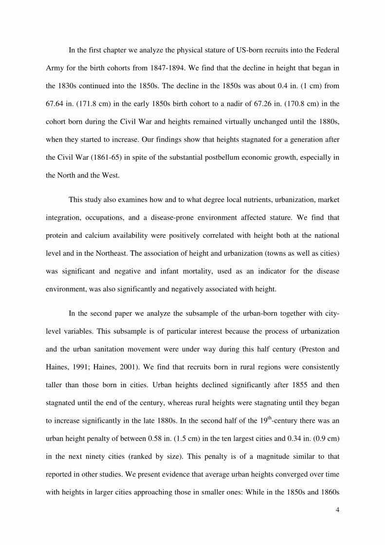
In the first chapter we analyze the physical stature of US-born recruits into the Federal

Army for the birth cohorts from 1847-1894. We find that the decline in height that began in

the 1830s continued into the 1850s. The decline in the 1850s was about 0.4 in. (1 cm) from

67.64 in. (171.8 cm) in the early 1850s birth cohort to a nadir of 67.26 in. (170.8 cm) in the

cohort born during the Civil War and heights remained virtually unchanged until the 1880s,

when they started to increase. Our findings show that heights stagnated for a generation after

the Civil War (1861-65) in spite of the substantial postbellum economic growth, especially in

the North and the West.

This study also examines how and to what degree local nutrients, urbanization, market

integration, occupations, and a disease-prone environment affected stature. We find that

protein and calcium availability were positively correlated with height both at the national

level and in the Northeast. The association of height and urbanization (towns as well as cities)

was significant and negative and infant mortality, used as an indicator for the disease

environment, was also significantly and negatively associated with height.

In the second paper we analyze the subsample of the urban-born together with city-

level variables. This subsample is of particular interest because the process of urbanization

and the urban sanitation movement were under way during this half century (Preston and

Haines, 1991; Haines, 2001). We find that recruits born in rural regions were consistently

taller than those born in cities. Urban heights declined significantly after 1855 and then

stagnated until the end of the century, whereas rural heights were stagnating until they began

to increase significantly in the late 1880s. In the second half of the 19th-century there was an

urban height penalty of between 0.58 in. (1.5 cm) in the ten largest cities and 0.34 in. (0.9 cm)

in the next ninety cities (ranked by size). This penalty is of a magnitude similar to that

reported in other studies. We present evidence that average urban heights converged over time

with heights in larger cities approaching those in smaller ones: While in the 1850s and 1860s

5

heights decreased with city size at a decreasing rate, in the late 19th-century we find this

relationship to be inversely U-shaped with largest heights in cities of about 250,000

inhabitants.

City dwellers’ height was positively correlated with expansion of the railroad network

because it led to increased market integration, which decreased the price and increased the

quality of the food that city dwellers purchased and consumed, and this improvement in their

nutrition soon translated into a height increase. Since real wages determined one’s quality of

life (the quality of one’s food and shelter, chiefly), their level was positively, and the death

rate negatively, correlated with height. Industrialization, too, as measured by the share of the

urban population working in the manufacturing sector, was negatively correlated with stature

because the working conditions and disease environment in factories compared unfavorably

with those of small-scale, rural manufacturing (Costa and Steckel, 1997).

The third paper investigates occupational mobility, occupational height premiums, and

family-level correlates of height. Drawing on the North Atlantic Population Project’s 1880

manuscript census, which enabled us to link data on recruits with data on their families, we

find that occupational mobility was on the rise during the period under consideration. Sons of

farmers were most likely to hold the same job as their father, followed by laborers, skilled

workers, upper-level white-collar workers, and semi-skilled workers compared with lower-

level white-collar workers.

We find that when controlling for the son’s instead of the father’s occupation we

overestimate the heights of all occupational categories except for that of skilled workers, but

only by at most 0.5%, or about 0.40 in. (1.0 cm). In the absence of information on the father’s

occupation, using the son’s as a proxy leads to a very small bias; the signs and significance of

all other coefficients remain unchanged. This finding should come as good news to

researchers who use this son-for-father proxy in anthropometric studies.

6

Our analysis of family-level correlates of height reveals that the number of siblings in

a household and being born in an urban area was negatively associated with height, whereas

having a father who was a farmer conveyed a height premium. These results (with the

exception of occupational categories) corroborate our findings in the preceding two papers

even when we control for family-level variables. The fact that the average height of recruits

whose parents were foreign-born did not differ significantly from that of other recruits (who

had native-born parents) suggests that living standards in the US at that time were so

beneficial for growth that it took just one generation for heights to reach American levels.

While these three papers compose a single dissertation, it was the author’s intention

that each of the three be independent of the others. This approach obliges a certain amount of

repetition in the data and methodological sections; those who read more than any one of the

three are therefore encouraged to skip passages rendered redundant by preceding discussions

of the same materials. In any case, it is recommended that these readers begin with the first

paper, because it draws on the full sample of recruits in order to present an overview of height

trends and levels, whereas the second and third papers use subsamples linked with city-level

and family-level data.

7

References

Atack, Jeremy, and Fred Bateman. 1984. “Self-Sufficiency and the Marketable Surplus in

the Rural North, 1860.” Agricultural History, 58 (3): 296-313.

Condran, Gretchen A., and Eileen Crimmins-Gardner. 1980. “Mortality differentials

between rural and urban areas of states in the northeastern United States 1890–1900.” Journal

of Historical Geography, 6 (2): 179-202.

Costa, Dora, and Richard Steckel. 1997. “Long-Term Trends in Health, Welfare, and

Economic Growth in the United States.” In: Health and Welfare during Industrialization, ed.

Richard Steckel and Roderick Floud, 47-90. Cambridge, MA: National Bureau of Economic

Research, Inc.

Davis, Joseph H. 2004. “An Annual Index of U.S. Industrial Production, 1790-1915.”

Quarterly Journal of Economics, 119: 1177-1215.

Fogel, Robert. 1994. “Economic Growth, Population Theory, and Physiology: the Bearing of

Long-term Processes on the Making of Economic Policy.” American Economic Review, 84:

369–395.

Haines, Michael. 2001. “The Urban Mortality Transition in the United States, 1800-1940.”

Annales de démographie historique, 101 (1): 33-64.

James, John. 1983. “Structural Changes in American Manufacturing, 1850-1890.” The

Journal of Economic History, 43 (2): 433-459.

Johnston, Louis D., and Samuel H. Williamson. 2008. "What Was the U.S. GDP Then?"

Measuring Worth. http://www.measuringworth.org/usgdp/ (accessed September 27, 2009).

Komlos, John. 1987. “The Height and Weight of West Point Cadets: Dietary Change in

Antebellum America.” The Journal of Economic History, 47: 897-927.

Komlos, John. 2009. “Anthropometric history: an overview of a quarter century of research.”

Anthropologischer Anzeiger; Bericht über die biologische-anthropologische Literatur, 67 (4):

341-356.

Komlos, John, and Peter A. Coclanis. 1995. “Nutrition and Economic Development in Post-

Reconstruction South Carolina: An Anthropometric Approach.” Social Science History, 19

(1): 91-115.

Lewis, Frank. 1979. “Explaining the Shift of Labor from Agriculture to Industry in the

United States: 1869 to 1899.” The Journal of Economic History, 39 (3): 681-698.

8

Margo, Robert, and Richard Steckel. 1983. “Heights of Native Born Northern Whites

during the Antebellum Period.” Journal of Economic History, 43: 167-184.

Preston, Samuel H., and Michael Haines. 1991. Fatal Years: Child Mortality in the Late

Nineteenth-Century America. Princeton, NJ: Princeton University Press.

Rosenbloom, Joshua. 1990. “Labor Market Institutions and the Geographic Integration of

Labor Markets in the Late Nineteenth-Century United States.” The Journal of Economic

History, 50 (2): 440-441.

Silventoinen, Karri. 2003. “Determinants of variation in adult body height.” Journal of

Biosocial Science, 35: 263-285.

Steckel, Richard. 1995. “Stature and the Standard of Living.” Journal of Economic

Literature, 33 (4): 1903-1940.

Steckel, Richard. 2009. “Heights and human welfare: Recent developments and new

directions.” Explorations in Economic History, 33 (4): 1-23.

Steckel, Richard, and Donald Haurin. 1994. “Health and Nutrition in the American

Midwest: Evidence from the Height of Ohio National Guardsmen, 1850-1910.” In: Stature,

Living Standards, and Economic Development: Essays in Anthropometric History, ed. John

Komlos, 117-128. Chicago: The University of Chicago Press.

Sunder, Marco. 2007. “Passports and Economic Development: An Anthropometric History

of the U.S. Elite in the Nineteenth Century.” PhD diss. University of Munich.

Waaler, Hans. 1984. “Height, Weight and Mortality: The Norwegian Experience.” Acta

Medica Scandinavica, Supplement, 679: 1-51.

Waterlow, John. 1994. “Summary of Causes and Mechanisms of Linear Growth

Retardation.” European Journal of Clinical Nutrition, 48: (Suppl 1): S210.

Weiss, Thomas. 1992. “U.S. Labor Force Estimates and Economic Growth, 1800-1860,” In:

American Economic Growth and Standards of Living Before the Civil War, ed. Robert

Gallman and John Wallis, 19-75. Chicago: University of Chicago Press.

Williamson, Jeffrey G. 1975. “The Relative Costs of American Men, Skills, and Machines:

A Long View.” Discussion Paper, No. 289-75. Institute for Research on Poverty, University

of Wisconsin-Madison.

Williamson, Jeffrey G. 1976. “American Prices and Urban Inequality Since 1820.” The

Journal of Economic History, 36 (2): 303-333.

9

1. The Postbellum Continuation of the Antebellum Puzzle:

Stature in the US, 1847 - 1894

ABSTRACT

This paper explores whether the antebellum decline in heights continued in the post-Civil War

period by using a data set of more than 58,000 US Army recruits born between 1847 and

1894. The main finding is that heights continued to decline during the Civil War by about 0.4

in. (1.0 cm) and stagnated for an extended period of time before they began to increase among

the birth cohorts of the late 1880s. Height was positively correlated with proximity to protein-

rich nutrients during childhood and with geographic mobility and was negatively correlated

with urbanization, and infant mortality rates.

10

1.1 Introduction

Economic historians, using height as an indicator of the biological standard of living, have

discovered anomalies in history such as the Antebellum Puzzle: a pattern of declining stature

among American men despite a growing economy in the years before the Civil War (Komlos,

1987; Fogel, 1994; Steckel, 1995). Much work has been done in order to understand the

causes of the decline in the biological standard of living prior to the Civil War, but the post-

bellum epoch has received less attention with the exception of Steckel and Haurin (1994) on

Ohio National Guardsmen, Komlos and Coclanis (1995) on Citadel students, Sunder (2007)

on passport applicants, Maloney and Carson (2008) on Ohio prison inmates, and Hiermeyer’s

(2008) continuation of Komlos’s (1987) analysis of West Point Cadets. Therefore it is to this

period that we have turned our attention. We analyze the physical stature of 58,512 US Army

recruits who enlisted between 1898 and 1912 and were born from 1847 to 1894, together with

explanatory variables from the US aggregate census of 1880.

1.1.1 Historical Background

The period from 1850 to 1890 is of great interest not only because of the Civil War but

because it was a time of rapid growth in Gross National Product (GNP), industrial production,

urbanization, transportation, and communication, all of which dramatically changed the US

economy. The history of physical stature enables us to assess the Civil War’s impact on the

US population, because height data supplement the scanty evidence derived from

conventional measures of the standard of living.

Civil War and Spanish American War

The Civil War, which lasted from April of 1861 to April of 1865 and its burden manifested

itself in the destruction of property, inflation, a rise in foreign-exchange prices (declining

greenbacks making imports more expensive), and falling cotton prices all of which hurt the

11

South more than the North (Hughes and Cain, 2002). By the end of the war wealth in the

South had fallen by 30% while wealth in the North had increased by 50% (between 1860 and

1870). Between 1860 and 1866 farm real estate fell by 50% and the number of livestock had

dropped between 32 and 42% in the South (Sellers, 1927).

Our enlistment period ranges from 1898 to 1912 including the Spanish American War

which lasted from April until August of 1898. Congress passed the Mobilization Act in 1898,

thereby increasing the size of the Army and when President McKinley called for volunteers,

the Army’s ranks soon swelled by 182,687 men (Smith, 1994; Crawford, Hayes, and

Sessions, 1998).

Conventional Economic Indicators

Conventional economic indicators were constructed and periodically refined by Robert

Gallman for the period from 1834 to 1909 (Gallman, 1960, 1966, 2000; Rhode, 2002). We

use Rhode’s (2002) corrected and revised estimates of Gallman’s (1966) annual GNP figures.

Between 1847 and 1894 GNP (excluding inventory changes in 1860 dollars) grew more than

fourfold, from $2.4 to $13.6 billion dollars. GNP per capita increased by 74% with the US

population more than doubling. The decade ending in 1869, which included the Civil War,

shows a 4% decline in output per capita with a hiatus from 1860 to 1868 which was especially

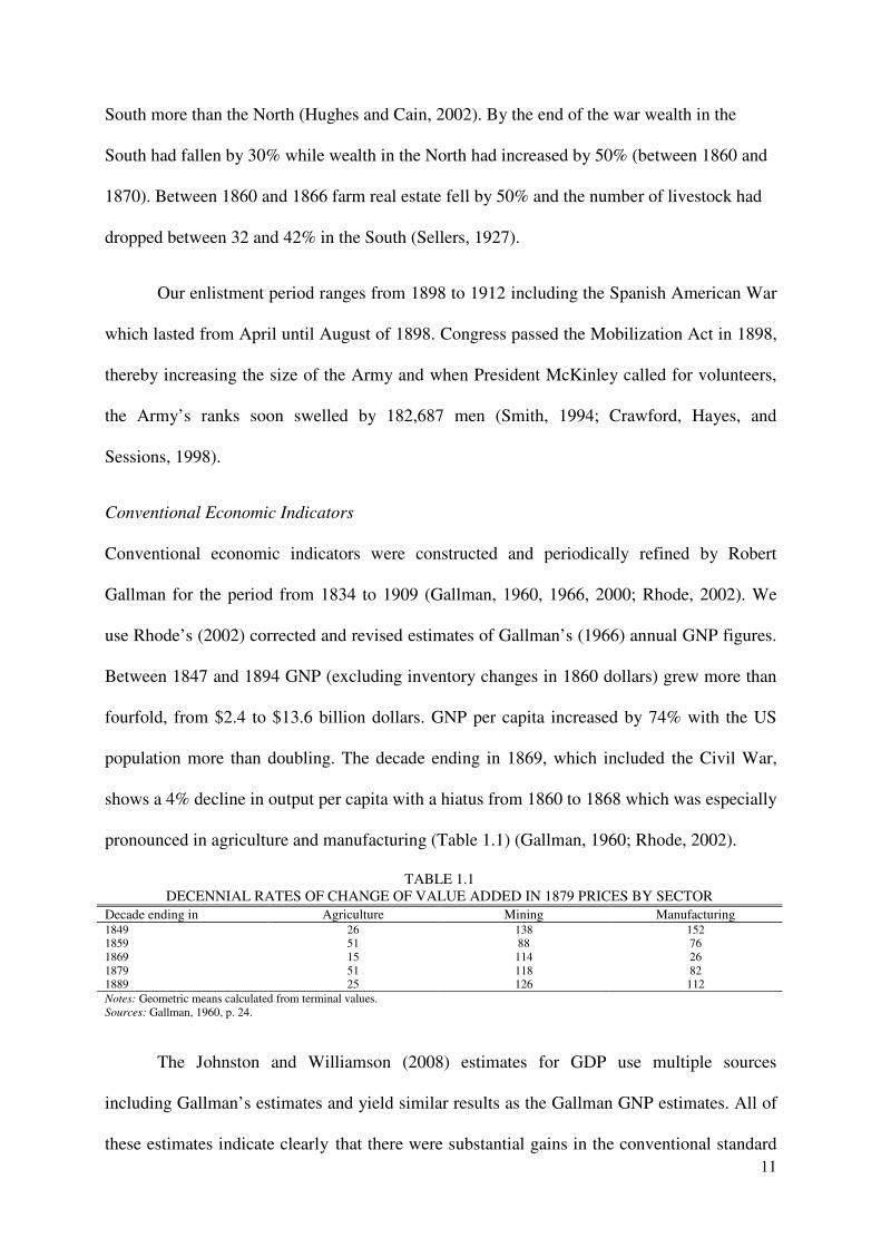
pronounced in agriculture and manufacturing (Table 1.1) (Gallman, 1960; Rhode, 2002).

TABLE 1.1 DECENNIAL RATES OF CHANGE OF VALUE ADDED IN 1879 PRICES BY SECTOR

Decade ending in Agriculture Mining Manufacturing 1849 26 138 152 1859 51 88 76 1869 15 114 26 1879 51 118 82 1889 25 126 112 Notes: Geometric means calculated from terminal values. Sources: Gallman, 1960, p. 24.

The Johnston and Williamson (2008) estimates for GDP use multiple sources

including Gallman’s estimates and yield similar results as the Gallman GNP estimates. All of

these estimates indicate clearly that there were substantial gains in the conventional standard

12

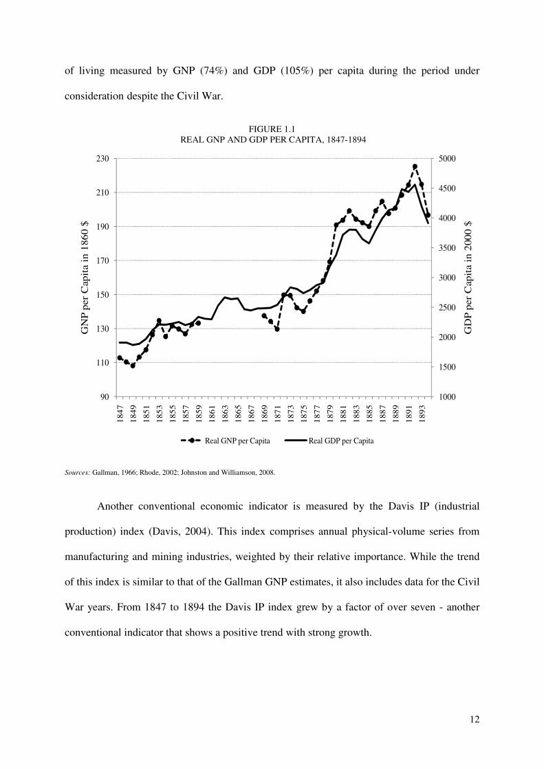
of living measured by GNP (74%) and GDP (105%) per capita during the period under

consideration despite the Civil War.

FIGURE 1.1 REAL GNP AND GDP PER CAPITA, 1847-1894

1000

1500

2000

2500

3000

3500

4000

4500

5000

90

110

130

150

170

190

210

230

184

7

184

9

185

1

185

3

185

5

185

7

185

9

186

1

186

3

186

5

186

7

186

9

187

1

187

3

187

5

187

7

187

9

188

1

188

3

188

5

188

7

188

9

189

1

189

3

GD

P p

er C

apit

a in

200

0 $

GN

P p

er C

apit

a in

186

0 $

Real GNP per Capita Real GDP per Capita

Sources: Gallman, 1966; Rhode, 2002; Johnston and Williamson, 2008.

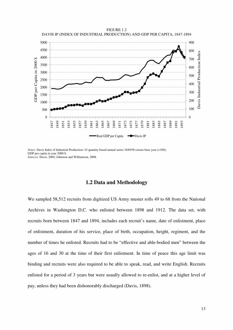
Another conventional economic indicator is measured by the Davis IP (industrial

production) index (Davis, 2004). This index comprises annual physical-volume series from

manufacturing and mining industries, weighted by their relative importance. While the trend

of this index is similar to that of the Gallman GNP estimates, it also includes data for the Civil

War years. From 1847 to 1894 the Davis IP index grew by a factor of over seven - another

conventional indicator that shows a positive trend with strong growth.

13

FIGURE 1.2 DAVIS IP (INDEX OF INDUSTRIAL PRODUCTION) AND GDP PER CAPITA, 1847-1894

0

100

200

300

400

500

600

700

800

900

0

500

1000

1500

2000

2500

3000

3500

4000

4500

5000

18

47

18

49

18

51

18

53

18

55

18

57

18

59

18

61

18

63

18

65

18

67

18

69

18

71

18

73

18

75

18

77

18

79

18

81

18

83

18

85

18

87

18

89

18

91

18

93

Dav

is I

ndu

stri

al P

rod

uct

ion

In

dex

GD

P p

er C

apit

a in

20

00

$

Real GDP per Capita Davis IP

Notes: Davis Index of Industrial Production: 43 quantity based annual series 1849/50 census base year (=100); GDP per capita in year 2000 $. Sources: Davis, 2004; Johnston and Williamson, 2008.

1.2 Data and Methodology

We sampled 58,512 recruits from digitized US Army muster rolls 49 to 68 from the National

Archives in Washington D.C. who enlisted between 1898 and 1912. The data set, with

recruits born between 1847 and 1894, includes each recruit’s name, date of enlistment, place

of enlistment, duration of his service, place of birth, occupation, height, regiment, and the

number of times he enlisted. Recruits had to be “effective and able-bodied men” between the

ages of 16 and 30 at the time of their first enlistment. In time of peace this age limit was

binding and recruits were also required to be able to speak, read, and write English. Recruits

enlisted for a period of 3 years but were usually allowed to re-enlist, and at a higher level of

pay, unless they had been dishonorably discharged (Davis, 1898).

14

All recruits born outside of the continental US and those for whom there is no record

of the state where they were born were excluded from our analysis (N=68) because we cannot

control for their net-nutritional experience while they were growing up. This exclusion also

applies to observations above a physiologically plausible maximum height of 78 in. (198.1

cm) (N=41). We also excluded recruits under the age of 18 (N=56); although the Army

permitted boys as young as 16 to enlist if they had parental consent, it was likely that they

were too far from their maximal adult height2 for our purposes (Davis, 1898; Tanner, 1978).

Also excluded were recruits over the age of 50 (N=102), because by that age there is usually

some loss of height, and therefore inclusion of these data would have biased our estimation

(Komlos, 2004b). These exclusions reduced the sample to 58,512 US-born recruits, between

the ages of 18 and 50, with a minimum height of 63.79 in. (162.0 cm) and a maximum height

of 78 in. (198.1 cm).

The recruits were assigned state and county National Historical Geographic

Information System (NHGIS) codes that identify a county. This geo-coding process allowed

us to combine the enlistment records with county-level statistics from the 1880 US Census in

order to relate information on agriculture, demographics, and wages to the recruits’ places of

birth (Minnesota Population Center, 2004). For county-level analysis we excluded all those

recruits for whom the county of birth could not be identified (38.2%, N=22,362), but we

included them in our estimate of national height trends. These recruits were on average 0.27

in. (0.7 cm) taller than those who could be geo-coded (1% level of significance). This height

advantage could be explained by the fact that those who could not be geo-coded tend to have

been born in remote rural regions, and in such regions nutrition was often better than in more

populated areas (Komlos, 1987). In order to combine information from the US Census with

the recruit data set it was necessary to correct the spelling of place names in about 8.1%

2 In the 19th century, maximal adult height was often not reached until about the age of 23 (Komlos, 2004b).

15

(N=3,772) of the cases. Recruits born in counties that merged with other counties or changed

names were assigned to the successor counties. At the time of enlistment a recruit had a

choice between identifying the town or the county of his birth; this latitude complicated our

task when a town and a county shared the name in question, but where the town was not

located in the county by the same name. These cases therefore could not be county-coded, and

were used only in our state-level analysis.

County-level census data are problematic because height reflects the long-term

environmental conditions during periods of growth, whereas census data, being decadal, can

provide only a snapshot of conditions at one particular time. We assume that county-level

census variables follow an autocorrelated process: for instance, that in 1880 each county’s

agricultural output is correlated with its past output. Since data from the 1880 census are more

satisfactory than those of any previous census year and since about 98% of our county-coded

recruits were still growing in 1880, we chose this census year for our analysis. We must

further assume that the county of birth had an effect on the height of recruits because there is

no information in the muster rolls on places other than those of birth and enlistment. Further

hindering our analysis is the fact that county-level statistics on most of the variables of

interest say little about the distribution of food or wages among individuals or about their

choice of consumption bundles. Data on these variables just indicate the potential availability

of nutrients in a given county.

Adult heights of a homogenous population are, as a rule, asymptotically normally

distributed (Tanner, 1978; Bogin, 1999). The Army’s minimum height requirements (MHR)

could introduce an upward bias in our sample heights, if we were to analyze the data using

OLS. Visual inspection of the height distribution permits one to identify the MHR, which is

crucial to estimate regressions consistently. The distribution above the MHR should resemble

16

a truncated normal distribution, whereas the existence of an underrepresented range, called

the shortfall, means that the truncation is imperfect (Komlos, 2004b).

A measurement error in the height variable is very likely, on account of heaping not

only at the MHR, where there was probably an upward bias due to rounding but also at

integer heights3. Signs of heaping are abnormally high frequencies of integer heights (Figure

1.3), whereas the distribution of non-integer heights is much smoother. In any case,

symmetric heaping would not seriously bias our results (Komlos, 2004a).

Figure 1.3 indicates that there was a minimum height requirement (MHR) of 64 in.

(162.6 cm) to join the military, therefore truncated maximum likelihood estimation (TMLE) is

used for consistent estimates and all regression analysis is carried out with TMLE (Komlos,

2004b). Some models are estimated with a constrained standard deviation of today’s adult

population, which is 2.7 in. (6.86 cm), according to Frisancho (1990) and Cole (2000). The

advantage of restricting the standard deviation of height is increased precision and reduced

variance, but it might bring about a trade-off between bias and precision of the estimator. That

is why we present estimation both ways, with and without constraining the standard deviation

of the height distribution. Simulations show that the restriction’s effect on time trends in

heights and explanatory variables is minimal but the effect on levels can be substantial

(A’Hearn, 2004; Komlos, 2004a).

The spatial distribution of our sample is different from the distribution of white males

between the ages of 15 and 49 in the 1880 census: the West is underrepresented by 3.5

percentage points, the Midwest by 2.3 percentage points, the South by 6.1 percentage points,

whereas the Northeast is overrepresented by 12.6 percentage points (Figure 1.4). This is

factored in by the use of weights in the calculation of national height levels.

3 Only 2% of the heights in enlistment records were reported in fractions smaller than a quarter inch.

17

FIGURE 1.3 RELATIVE FREQUENCY OF HEIGHTS:

ENLISTMENT YEARS 1898-1912

0,0

1,0

2,0

3,0

4,0

5,0

6,0

7,0

63

63

,5 64

64

,5 65

65

,5 66

66

,5 67

67

,5 68

68

,5 69

69

,5 70

70

,5 71

71

,5 72

72

,5 73

73

,5 74

Rel

ati

ve

Fre

qu

enci

es o

f H

eigh

ts

Height in Inches

Sources: See the text.

FIGURE 1.4 DISTRIBUTION OF RECRUITS BY CENSUS REGION

Notes: Census white males is the number of white males aged between 15 and 49 in each census region divided by the number of white males between 15 and 49 nationwide in 1880. Sources: Minnesota Population Center, 2004.

0

0,05

0,1

0,15

0,2

0,25

0,3

0,35

0,4

0,45

West Midwest South Northeast

Rel

ativ

e F

requ

ency

Census White Males Sample

18

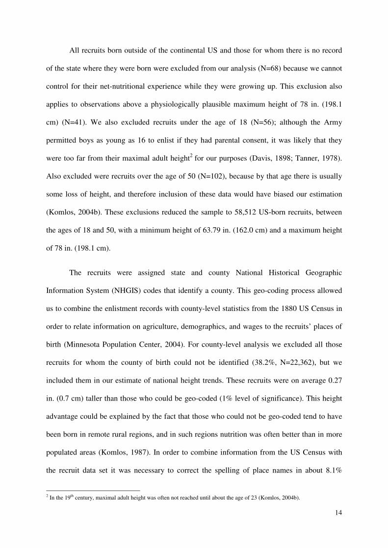
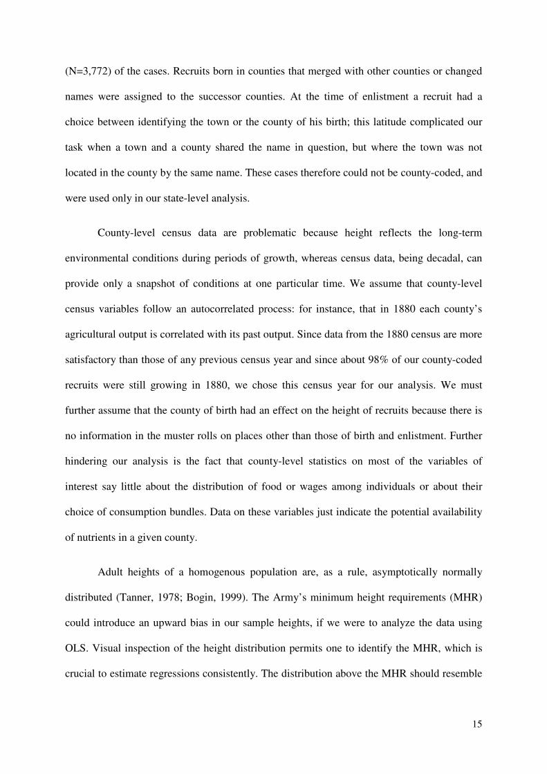
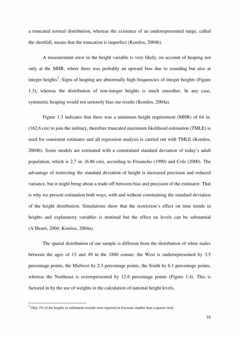
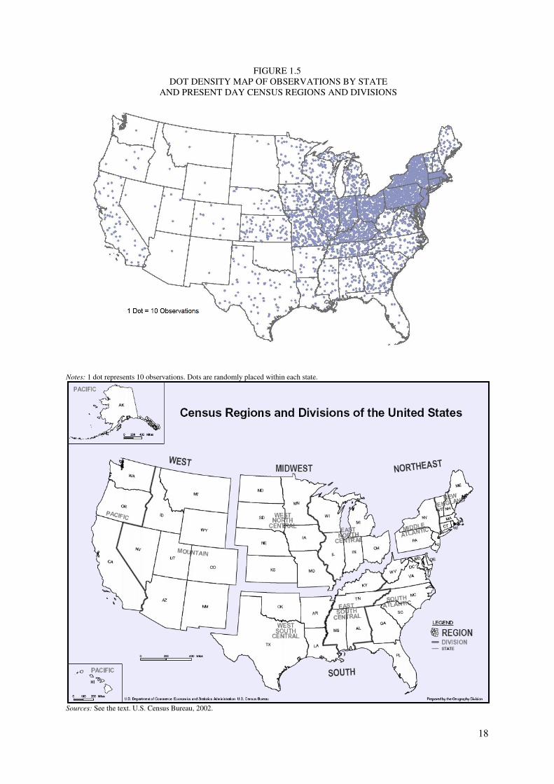
FIGURE 1.5 DOT DENSITY MAP OF OBSERVATIONS BY STATE

AND PRESENT DAY CENSUS REGIONS AND DIVISIONS

Notes: 1 dot represents 10 observations. Dots are randomly placed within each state.

Sources: See the text. U.S. Census Bureau, 2002.

19

TABLE 1.2 DESCRIPTIVE STATISTICS

Full Data Set Geo-coded Data Set Variable µ σ Min Max N µ σ Min Max N

Birth Cohorts 1847-1854 0.01 0.08 0.00 1.00 381 0.01 0.08 0.00 1.00 296

1855-1859 0.01 0.10 0.00 1.00 545 0.01 0.10 0.00 1.00 415 1860-1864 0.02 0.15 0.00 1.00 1,415 0.03 0.16 0.00 1.00 1,121 1865-1869 0.08 0.27 0.00 1.00 4,699 0.09 0.28 0.00 1.00 3,636 1870-1874 0.22 0.41 0.00 1.00 12,842 0.24 0.43 0.00 1.00 9,935 1875-1879 0.50 0.50 0.00 1.00 29,048 0.52 0.50 0.00 1.00 21,608 1880-1884 0.12 0.32 0.00 1.00 6,742 0.09 0.27 0.00 1.00 3,787

1885-1889 0.04 0.18 0.00 1.00 2,062 0.02 0.13 0.00 1.00 720 1890-1894 0.01 0.11 0.00 1.00 778 0.01 0.07 0.00 1.00 312 West 0.02 0.14 0.00 1.00 1,215 0.02 0.14 0.00 1.00 798 Midwest 0.34 0.47 0.00 1.00 19,919 0.34 0.47 0.00 1.00 14,158 South 0.26 0.44 0.00 1.00 15,080 0.22 0.41 0.00 1.00 9,150 Northeast 0.38 0.49 0.00 1.00 22,160 0.42 0.49 0.00 1.00 17,720

Pacific 0.02 0.12 0.00 1.00 893 0.02 0.13 0.00 1.00 665 Mountain 0.01 0.07 0.00 1.00 322 0.00 0.06 0.00 1.00 133 West North C. 0.10 0.30 0.00 1.00 5,991 0.09 0.29 0.00 1.00 3,973 West South C. 0.03 0.16 0.00 1.00 1,631 0.02 0.15 0.00 1.00 948 East North C. 0.24 0.43 0.00 1.00 13,928 0.24 0.43 0.00 1.00 10,185 East South C. 0.11 0.32 0.00 1.00 6,613 0.1 0.31 0.00 1.00 4,349 Middle Atlantic 0.28 0.45 0.00 1.00 16,177 0.31 0.46 0.00 1.00 12,984

South Atlantic 0.12 0.32 0.00 1.00 6,836 0.09 0.29 0.00 1.00 3,853 New England 0.10 0.30 0.00 1.00 5,983 0.11 0.32 0.00 1.00 4,736 Laborer 0.21 0.41 0.00 1.00 12,309 0.21 0.41 0.00 1.00 8,821 Semi-skilled 0.37 0.48 0.00 1.00 21,393 0.37 0.48 0.00 1.00 15,304 Skilled 0.20 0.40 0.00 1.00 11,751 0.21 0.41 0.00 1.00 8,823 Farmer 0.12 0.33 0.00 1.00 7,211 0.11 0.31 0.00 1.00 4,498

Lower w. c. 0.07 0.26 0.00 1.00 4,301 0.08 0.27 0.00 1.00 3,219 Upper w. c. 0.03 0.16 0.00 1.00 1,586 0.03 0.17 0.00 1.00 1,180 Mover 0.54 0.50 0.00 1.00 31,595 0.51 0.50 0.00 1.00 21,205 Age 24.18 4.94 18.0 50.0 58,512 24.17 4.92 18.00 50.00 41,830 Age 18 0.05 0.22 0.00 1.00 3,064 0.05 0.22 0.00 1.00 2,139 Age 19 0.05 0.21 0.00 1.00 2,733 0.05 0.21 0.00 1.00 2,029

Age 20 0.03 0.18 0.00 1.00 2,008 0.04 0.19 0.00 1.00 1,506 Age 21 0.23 0.42 0.00 1.00 13,672 0.23 0.42 0.00 1.00 9,627 Age 22-50 0.63 0.48 0.00 1.00 37,054 0.63 0.48 0.00 1.00 26,529 Enlistment Years 1898 0.45 0.50 0.00 1.00 20,191 0.45 0.50 0.00 1.00 16,680 1899 0.28 0.45 0.00 1.00 12,439 0.27 0.45 0.00 1.00 10,082

1900 0.28 0.45 0.00 1.00 12,395 0.28 0.45 0.00 1.00 10,189 1901 0.09 0.29 0.00 1.00 5,516 0.04 0.21 0.00 1.00 1,855 1902 0.05 0.23 0.00 1.00 3,191 0.03 0.17 0.00 1.00 1,231 1909 0.03 0.17 0.00 1.00 1,656 0.01 0.12 0.00 1.00 612 1910 0.02 0.13 0.00 1.00 983 0.01 0.09 0.00 1.00 359 1911 0.03 0.18 0.00 1.00 1,968 0.02 0.13 0.00 1.00 753 1912 0.01 0.05 0.00 1.00 173 0.00 0.04 0.00 1.00 69

Census Variables Rural 0.57 0.37 0.00 1.00 41,830 Town 0.12 0.17 0.00 0.92 41,830 Urban 0.31 0.40 0.00 1.00 41,830 Wheat p.c. 7.80 13.02 0.00 345.90 41,830 Milk cows p.c. 0.19 0.18 0.00 2.18 41,830

Pigs p.c. 0.70 0.89 0.00 7.30 41,830 Wages 315.95 95.50 25.00 1112.27 41,830 Infant mortality 12.04 2.57 6.63 17.05 41,713 Railroad miles 391,137.40 207,823.40 20,998.00 756,239.00 41,713

Notes: North C. is North Central. South C. is South Central. Laborer includes those with unknown occupations. w. c. is white-collar. Skilled is skilled worker. Semi-skilled is semi-skilled worker. A mover enlisted in a state other than his state of birth. P.c. is per capita. Wheat is measured in 100 bushels. Wages are annual manufacturing wages per manufacturing worker. Infant mortality is measured in deaths per 1,000 births. Railroad miles are miles in a state completed as of June 1st 1880.Those in the geo-coded data set could be assigned to their counties of birth. Rural is the proportion of county inhabitants living in places with fewer than 2,500, Town with more than 2,500 and fewer than 25,000, and Urban with more than 25,000 inhabitants. Sources: See the text.

20

We begin by estimating time trends of height in the sample with controls for standard

census regions and divisions of birth. Thereafter we estimate trends in individual census

regions and divisions separately in order to account for spatial differences in levels and trends.

In the second section we include county-level variables to control for nutrient availability,

urbanization, socio-economic background, geographic mobility, transportation access, infant-

mortality rates, and manufacturing wages.

1.3 Results

1.3.1 Time Trends in Height

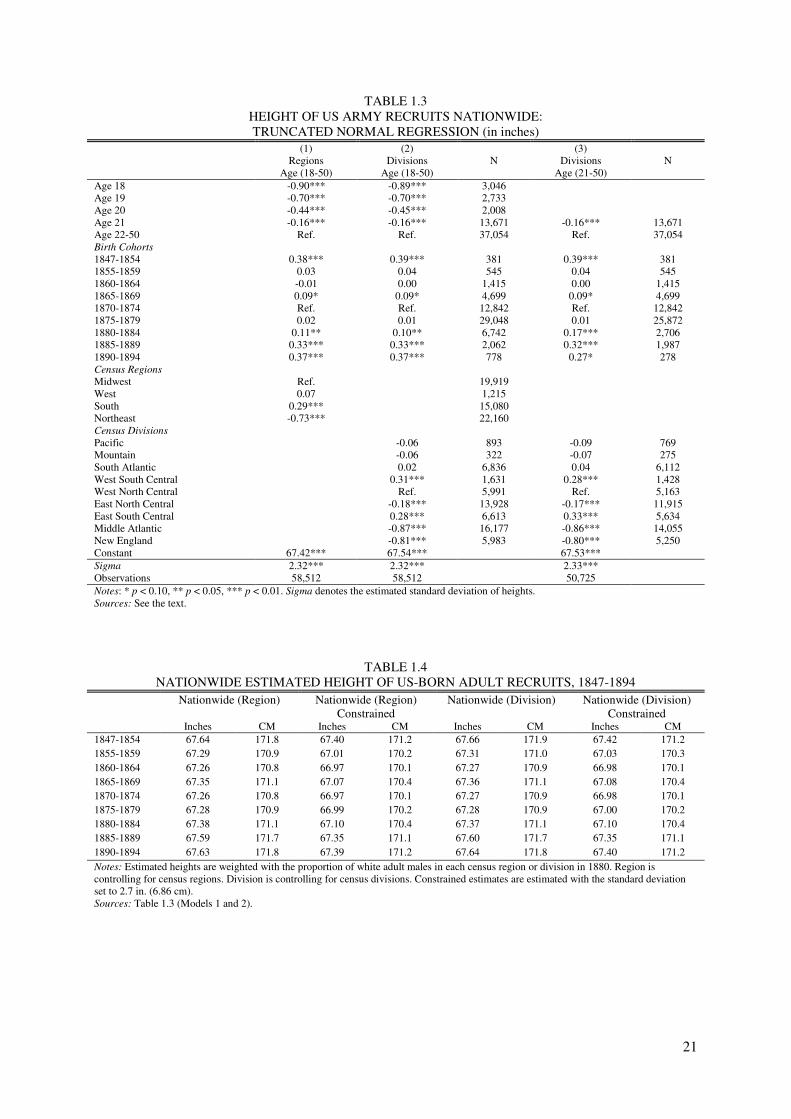
Heights declined in the 1850s, leveled off and stagnated until they increased in the 1880s.

This trend is identical when the sample is restricted to adults only and there is a height

gradient from the Northeast towards the South and the West4.

4 Those that enlisted during the Spanish American War were by 0.11 in. (0.3 cm) significantly shorter than recruits who

enlisted in times of peace. Estimating separate regressions by different precisions of reported height (quarter, half, and integer

inch) did not change results in Table 1.3.

21

TABLE 1.3 HEIGHT OF US ARMY RECRUITS NATIONWIDE: TRUNCATED NORMAL REGRESSION (in inches)

(1)

Regions Age (18-50)

(2) Divisions

Age (18-50) N

(3) Divisions

Age (21-50) N

Age 18 -0.90*** -0.89*** 3,046 Age 19 -0.70*** -0.70*** 2,733 Age 20 -0.44*** -0.45*** 2,008 Age 21 -0.16*** -0.16*** 13,671 -0.16*** 13,671 Age 22-50 Ref. Ref. 37,054 Ref. 37,054 Birth Cohorts 1847-1854 0.38*** 0.39*** 381 0.39*** 381 1855-1859 0.03 0.04 545 0.04 545 1860-1864 -0.01 0.00 1,415 0.00 1,415 1865-1869 0.09* 0.09* 4,699 0.09* 4,699 1870-1874 Ref. Ref. 12,842 Ref. 12,842 1875-1879 0.02 0.01 29,048 0.01 25,872 1880-1884 0.11** 0.10** 6,742 0.17*** 2,706 1885-1889 0.33*** 0.33*** 2,062 0.32*** 1,987 1890-1894 0.37*** 0.37*** 778 0.27* 278 Census Regions Midwest Ref. 19,919 West 0.07 1,215 South 0.29*** 15,080 Northeast -0.73*** 22,160 Census Divisions Pacific -0.06 893 -0.09 769 Mountain -0.06 322 -0.07 275 South Atlantic 0.02 6,836 0.04 6,112 West South Central 0.31*** 1,631 0.28*** 1,428 West North Central Ref. 5,991 Ref. 5,163 East North Central -0.18*** 13,928 -0.17*** 11,915 East South Central 0.28*** 6,613 0.33*** 5,634 Middle Atlantic -0.87*** 16,177 -0.86*** 14,055 New England -0.81*** 5,983 -0.80*** 5,250 Constant 67.42*** 67.54*** 67.53*** Sigma 2.32*** 2.32*** 2.33*** Observations 58,512 58,512 50,725 Notes: * p < 0.10, ** p < 0.05, *** p < 0.01. Sigma denotes the estimated standard deviation of heights. Sources: See the text.

TABLE 1.4 NATIONWIDE ESTIMATED HEIGHT OF US-BORN ADULT RECRUITS, 1847-1894

Nationwide (Region) Nationwide (Region)

Constrained Nationwide (Division) Nationwide (Division)

Constrained Inches CM Inches CM Inches CM Inches CM 1847-1854 67.64 171.8 67.40 171.2 67.66 171.9 67.42 171.2 1855-1859 67.29 170.9 67.01 170.2 67.31 171.0 67.03 170.3

1860-1864 67.26 170.8 66.97 170.1 67.27 170.9 66.98 170.1 1865-1869 67.35 171.1 67.07 170.4 67.36 171.1 67.08 170.4 1870-1874 67.26 170.8 66.97 170.1 67.27 170.9 66.98 170.1 1875-1879 67.28 170.9 66.99 170.2 67.28 170.9 67.00 170.2 1880-1884 67.38 171.1 67.10 170.4 67.37 171.1 67.10 170.4 1885-1889 67.59 171.7 67.35 171.1 67.60 171.7 67.35 171.1

1890-1894 67.63 171.8 67.39 171.2 67.64 171.8 67.40 171.2

Notes: Estimated heights are weighted with the proportion of white adult males in each census region or division in 1880. Region is controlling for census regions. Division is controlling for census divisions. Constrained estimates are estimated with the standard deviation set to 2.7 in. (6.86 cm). Sources: Table 1.3 (Models 1 and 2).

22

FIGURE 1.6 NATIONWIDE ESTIMATED HEIGHT OF US-BORN ADULT RECRUITS, 1847-1894

169,7

170,2

170,7

171,2

171,7

172,2

66,8

66,9

67,0

67,1

67,2

67,3

67,4

67,5

67,6

67,7

67,8

CM

Inch

es

Unconstrained Constrained

Notes: Estimated heights from Table 1.3 Model 2 weighted with the proportion of white adult males in each census division in 1880. Constrained estimates are estimated with the standard deviation set to 2.7 in. (6.86 cm). Sources: Table 1.4.

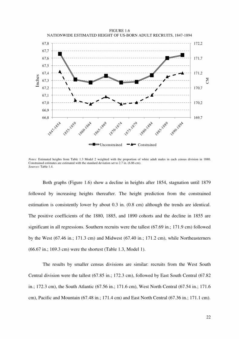
Both graphs (Figure 1.6) show a decline in heights after 1854, stagnation until 1879

followed by increasing heights thereafter. The height prediction from the constrained

estimation is consistently lower by about 0.3 in. (0.8 cm) although the trends are identical.

The positive coefficients of the 1880, 1885, and 1890 cohorts and the decline in 1855 are

significant in all regressions. Southern recruits were the tallest (67.69 in.; 171.9 cm) followed

by the West (67.46 in.; 171.3 cm) and Midwest (67.40 in.; 171.2 cm), while Northeasterners

(66.67 in.; 169.3 cm) were the shortest (Table 1.3, Model 1).

The results by smaller census divisions are similar: recruits from the West South

Central division were the tallest (67.85 in.; 172.3 cm), followed by East South Central (67.82

in.; 172.3 cm), the South Atlantic (67.56 in.; 171.6 cm), West North Central (67.54 in.; 171.6

cm), Pacific and Mountain (67.48 in.; 171.4 cm) and East North Central (67.36 in.; 171.1 cm).

23

The two shortest divisions were New England (66.73 in.; 169.5 cm) and Middle Atlantic

(66.67 in.; 169.3 cm) (Table 1.3, Model 2). The difference between the shortest and tallest

region was 1.02 in. (2.6 cm) and 1.18 in. (3.0 cm) among divisions.

Recruits from the South and in particular from the East South Central and the West

South Central divisions remained the tallest, despite the Civil War. This pattern corresponds

to the findings of Komlos (1987) that Southern-born West Point cadets were the tallest group

until the 1870s. Hiermeyer (2008) finds the Upper South, West, and (lower) South to be the

tallest and the Northeast to be the shortest regions. A’Hearn (1998) and Margo and Steckel

(1983) also find Westerners and Southerners to be taller than Northeasterners.

24

FIGURE 1.7 ESTIMATED HEIGHT OF US-BORN ADULT RECRUITS BY CENSUS DIVISION

AND REGION OF BIRTH, 1847-1894

Notes: Estimated heights from Models 1 and 2 (Table 1.3) averaged over birth cohorts 1847-1894. Sources: See the text.

25

TABLE 1.5 HEIGHT OF US ARMY RECRUITS BY CENSUS REGION:

TRUNCATED NORMAL REGRESSION (in inches) (1)

West N

(2) Midwest

N (3)

South N

(4) Northeast

N

Age 18 -0.59 66 -0.83*** 1,174 -1.09*** 688 -0.80*** 1,110 Age 19 -0.42 58 -0.57*** 933 -0.82*** 700 -0.71*** 1,039 Age 20 -0.03 47 -0.41*** 737 -0.57*** 518 -0.38*** 706 Age 21 0.33* 281 -0.14*** 4,900 -0.18*** 3,471 -0.18*** 4,992 Age 22-50 Ref. 763 Ref. 12,211 Ref. 9,703 Ref. 14,313 Birth Cohorts 1847-1864 0.85* 26 1865-1879 Ref. 1030 1880-1894 0.51** 159 1847-1854 0.14 76 -0.06 118 0.87*** 187 1855-1859 -0.13 137 0.13 154 0.11 247 1860-1864 0.10 430 0.13 358 -0.14 603 1865-1869 0.09 1,570 0.06 1,153 0.14* 1,886 1870-1874 Ref. 4,209 Ref. 3,214 Ref. 5,113 1875-1879 0.04 10,065 0.05 7,350 -0.04 10,958 1880-1884 0.06 2,522 0.17* 1,811 -0.02 2,277 1885-1889 0.35*** 708 0.37*** 675 0.16 622 1890-1894 0.49** 238 0.35** 247 0.25 267 Mountain -0.04 322 Pacific Ref. 893 Iowa 0.07 1,266 Nebraska 0.21 307 Kansas 0.20 968 Missouri -0.17 2,811 Wisconsin -0.05 896 Michigan -0.44*** 1,716 Illinois -0.22** 3,427 Indiana 0.08 3,154 Ohio -0.32*** 4,735 Minnesota Ref. 599 Dakota -0.11 76 Oklahoma 1.04*** 44 Arkansas 0.88*** 349 Texas 1.01*** 970 Louisiana 0.46** 268 Kentucky 0.78*** 3,662 Tennessee 1.03*** 1,923 Mississippi 0.89*** 343 Alabama 0.89*** 685 West-Virginia 0.89*** 668 Virginia 0.69*** 1,309 North Carolina 1.13*** 1,138 South Carolina 0.72*** 568 Georgia 0.69*** 1,358 Florida 0.70** 158 D.C. Ref. 340 Delaware -0.46 114 Maryland -0.20 1,093 New York 0.08* 7,635 Vermont 0.54*** 299 New Hampshire -0.03 271 Massachusetts -0.03 3,471 Connecticut 0.15 830 Rhode Island 0.14 503 Maine 0.52*** 609 New Jersey 0.03 1,626 Pennsylvania Ref. 6,916 Constant 67.32*** 67.57*** 66.97*** 66.66*** Sigma 2.28*** 2.28*** 2.30*** 2.34*** N 1,215 19,955 15,080 22,160 Notes: * p < 0.10, ** p < 0.05, *** p < 0.01. Sigma denotes the estimated standard deviation of heights. D.C. is Washington D.C. Dakota corresponds to North and South Dakota. Sources: See the text.

26

TABLE 1.6 ESTIMATED HEIGHT OF US-BORN ADULT RECRUITS BY CENSUS REGION, 1855-1894

Midwest South Northeast Inches CM Inches CM Inches CM

Unconstrained Estimation

1855-1859 67.26 170.8 67.87 172.4 66.79 169.6 1860-1864 67.48 171.4 67.86 172.4 66.54 169.0 1865-1869 67.48 171.4 67.8 172.2 66.82 169.7 1870-1874 67.38 171.1 67.73 172.0 66.68 169.4 1875-1879 67.42 171.2 67.79 172.2 66.64 169.3 1880-1884 67.44 171.3 67.9 172.5 66.66 169.3 1885-1889 67.74 172.1 68.11 173.0 66.84 169.8 1890-1894 67.87 172.4 68.08 172.9 66.93 170.0

Constrained Estimation

1855-1859 66.94 170.0 67.64 171.8 66.46 168.8 1860-1864 67.20 170.7 67.64 171.8 66.17 168.1 1865-1869 67.19 170.7 67.57 171.6 66.49 168.9 1870-1874 67.09 170.4 67.49 171.4 66.33 168.5 1875-1879 67.13 170.5 67.55 171.6 66.28 168.4 1880-1884 67.15 170.6 67.69 171.9 66.31 168.4 1885-1889 67.50 171.5 67.91 172.5 66.51 168.9 1890-1894 67.65 171.8 67.89 172.4 66.62 169.2

Notes: Estimated heights are weighted with the proportion of white adult males in each state in 1880. Constrained estimates are estimated with the standard deviation set to 2.7 in. (6.86 cm). Sources: Table 1.5.

FIGURE 1.8 ESTIMATED HEIGHT OF US-BORN ADULT RECRUITS BY CENSUS REGION,

1855-1894

167,6

168,1

168,6

169,1

169,6

170,1

170,6

171,1

171,6

172,1

172,6

173,1

66,0

66,2

66,4

66,6

66,8

67,0

67,2

67,4

67,6

67,8

68,0

68,2

1855 -1859

1860 -1864

1865 -1869

1870 -1874

1875 -1879

1880 -1884

1885 -1889

1890 -1894

CM

Inch

es

South South Constrained Midwest

Midwest Constrained Northeast Northeast Constrained

Notes: Estimated heights from Table 1.5 weighted with the proportion of white adult males in each state in 1880. Constrained estimates are estimated with the standard deviation set to 2.7 in. (6.86 cm). Sources: Table 1.6.

27

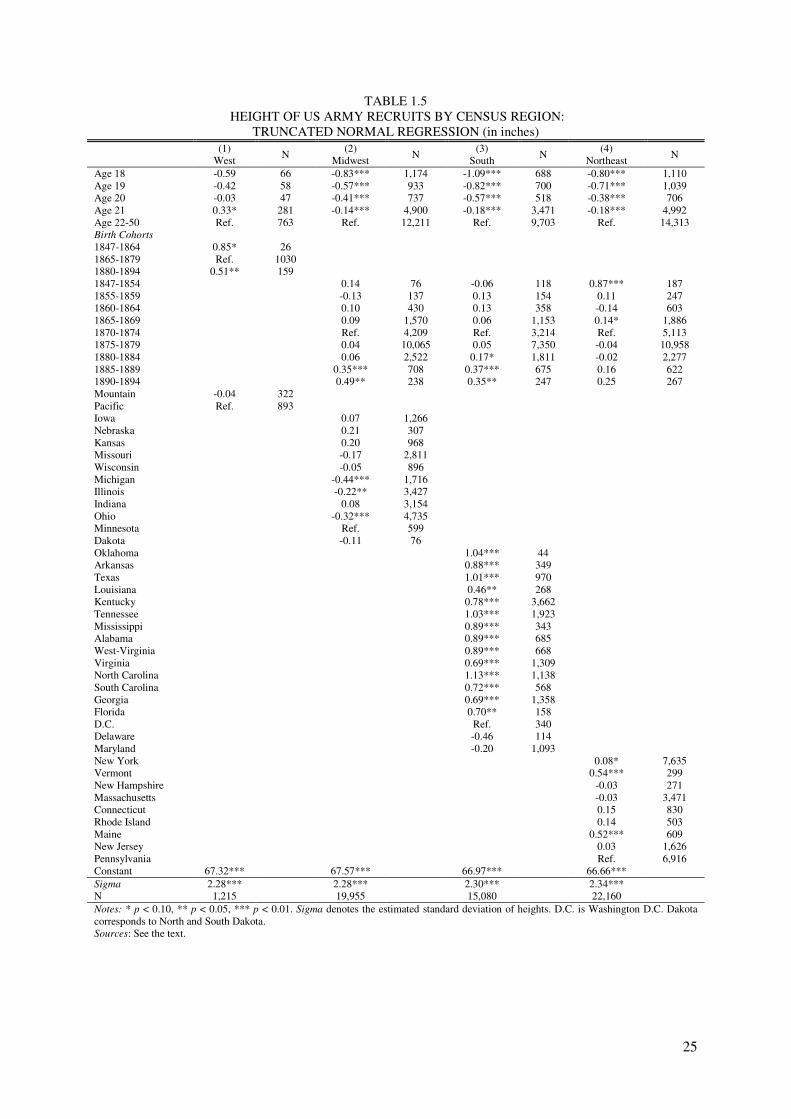
The trends over time differ by region: The South is the tallest region and experiences

stagnation until 1880, the Midwest is second with stagnation until 1885, trailed by the

Northeast with declines in the 1850s followed by stagnation (Table 1.5 and Figure 1.8). The

trends by census division are very heterogeneous (Tables 1.7 and 1.8; Figures 1.9 and 1.10).

The time dummy variables are divided into decades instead of quinquennia as above in order

to attain an adequate sample size for each period. The Pacific and Mountain divisions were

excluded because of their small sample size.

TABLE 1.7 HEIGHT OF US ARMY RECRUITS BY CENSUS DIVISION IN NORTHEAST AND MIDWEST:

TRUNCATED NORMAL REGRESSION (in inches) (1)

East North Central

N (2) Middle Atlantic

N (3) West North

Central

N (4) New

England

N

Age 18 -0.88*** 837 -0.92*** 832 -0.91*** 337 -0.72*** 278 Age 19 -0.53*** 664 -0.87*** 763 -0.79*** 269 -0.48** 276 Age 20 -0.48*** 512 -0.41*** 527 -0.32* 225 -0.48** 179 Age 21 -0.12** 3,330 -0.30*** 3,735 -0.19** 1,570 0.01 1,257 Age 22-50 Ref. 8,585 Ref. 10,320 Ref. 3,626 Ref. 3,993 Birth Cohorts 1847-1864 -0.07 476 0.05 749 0.26 167 0.28* 1865-1879 Ref. 11,041 Ref. 13,124 Ref 4,803 Ref. 1880-1894 0.12 2,411 0.10 2,304 0.20** 1,057 -0.01 Michigan -0.38*** 1,716 Illinois -0.16* 3,427 Wisconsin Ref. 896 Indiana 0.13 3,154 Ohio -0.27*** 4,735 New York 0.09* 7,635 Pennsylvania Ref. 6,916 New Jersey 0.03 1,626 Iowa 0.07 1,266 Minnesota Ref 599 Dakota -0.13 76 Nebraska 0.22 307 Kansas 0.2 968 Missouri -0.17 2,811 Vermont 0.02 299 New Hampshire -0.57*** 271 Maine Ref. 609 Massachusetts -0.56*** 3,471 Connecticut -0.38*** 830 Rhode Island -0.40** 503 Constant 67.54*** 66.67*** 67.62*** 67.15*** Sigma 2.30*** 2.35*** 2.25*** 2.31*** N 13,928 16,177 6,027 5,983 Notes: * p < 0.10, ** p < 0.05, *** p < 0.01. Sigma denotes the estimated standard deviation of heights. Dakota corresponds to North and South Dakota. Sources: See the text.

28

FIGURE 1.9 ESTIMATED HEIGHT OF US-BORN ADULT RECRUITS BY CENSUS DIVISION

IN NORTHEAST AND MIDWEST, 1847-1894

168,7

169,2

169,7

170,2

170,7

171,2

171,7

172,2

172,7

66,4

66,6

66,8

67,0

67,2

67,4

67,6

67,8

68,0

1847-1864 1865-1879 1880-1894

CM

Inch

es

West North Centra l East North Central

New England Middle Atlantic

Notes: Estimated heights from Table 1.7 weighted with the proportion of white adult males in each state in 1880. Sources: Table 1.9.

FIGURE 1.10 ESTIMATED HEIGHT OF US-BORN ADULT RECRUITS BY CENSUS DIVISION

IN THE SOUTH, 1847-1894

171,2

171,4

171,6

171,8

172,0

172,2

172,4

172,6

172,8

173,0

173,2

67,4

67,5

67,6

67,7

67,8

67,9

68,0

68,1

68,2

1847-1864 1865-1879 1880-1894

CM

Inch

es

East South Central West South Central South Atlantic

Notes: Estimated heights from Table 1.8 weighted with the proportion of white adult males in each state in 1880. Sources: Table 1.9.

29

TABLE 1.8 HEIGHT OF US ARMY RECRUITS BY CENSUS DIVISION IN THE SOUTH:

TRUNCATED NORMAL REGRESSION (in inches)

(1) South

Atlantic N

(2) West South

Central N

(3) East South

Central N

Age 18 -1.06*** 257 -0.59* 66 -1.29*** 365 Age 19 -0.80*** 280 -0.51* 78 -0.95*** 342 Age 20 -0.42** 187 0.06 59 -0.83*** 272 Age 21 -0.18** 1,496 0.04 404 -0.22** 1,571 Age 22-50 Ref. 4,616 Ref. 1,024 Ref. 4,063 Birth Cohorts 1847-1864 0.35** 368 -0.30 47 -0.33* 215 1865-1879 Ref. 5,352 Ref. 1,264 Ref. 5,101 1880-1894 0.20* 1,116 0.20 320 0.22** 1,297 West Virginia 0.93*** 668 Virginia 0.70*** 1,399 D. C. Ref. 340 Maryland -0.20 1,093 Delaware -0.48 114 North Carolina 1.16*** 1,138 South Carolina 0.75*** 568 Georgia 0.72*** 1,358 Florida 0.73** 158 Texas 0.12 970 Oklahoma 0.15 44 Arkansas Ref. 349 Louisiana -0.35* 268 Mississippi 0.00 343 Alabama Ref. 685 Tennessee 0.14 1,923 Kentucky -0.10 3,662 Constant 66.94*** 67.83*** 67.95*** Sigma 2.35*** 2.18*** 2.28*** N 6,836 1,631 6,613 Notes: * p < 0.10, ** p < 0.05, *** p < 0.01. Sigma denotes the estimated standard deviation of heights. D.C. is Washington D.C. Sources: See the text.

TABLE 1.9 ESTIMATED HEIGHT OF US-BORN ADULT RECRUITS BY CENSUS REGION,

1847-1894 Midwest & Northeast: East North Central Middle Atlantic West North Central New England Cohorts Inches CM Inches CM Inches CM Inches CM 1847-1864 67.27 170.9 66.68 169.4 67.82 172.3 67.04 170.3 1865-1879 67.34 171.0 66.64 169.3 67.56 171.6 66.75 169.6 1880-1894 67.46 171.3 66.74 169.5 67.75 172.1 66.75 169.5 South: South Atlantic West South Central East South Central Cohorts Inches CM Inches CM Inches CM 1847-1864 67.91 172.5 67.50 171.5 67.53 171.5 1865-1879 67.55 171.6 67.81 172.2 67.87 172.4 1880-1894 67.75 172.1 68.01 172.8 68.08 172.9

Notes: Estimated heights are weighted with the proportion of white adult males in each state in 1880. Sources: Tables 1.7 and 1.8.

30

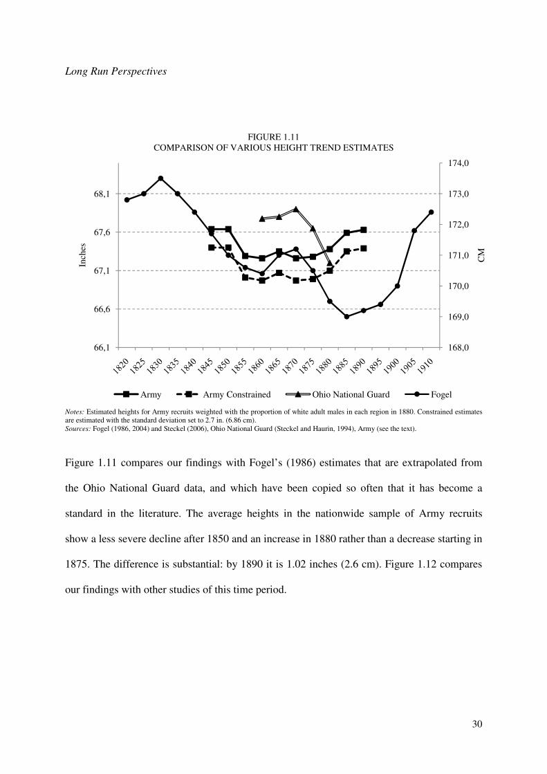
Long Run Perspectives

FIGURE 1.11 COMPARISON OF VARIOUS HEIGHT TREND ESTIMATES

Notes: Estimated heights for Army recruits weighted with the proportion of white adult males in each region in 1880. Constrained estimates are estimated with the standard deviation set to 2.7 in. (6.86 cm). Sources: Fogel (1986, 2004) and Steckel (2006), Ohio National Guard (Steckel and Haurin, 1994), Army (see the text).

Figure 1.11 compares our findings with Fogel’s (1986) estimates that are extrapolated from

the Ohio National Guard data, and which have been copied so often that it has become a

standard in the literature. The average heights in the nationwide sample of Army recruits

show a less severe decline after 1850 and an increase in 1880 rather than a decrease starting in

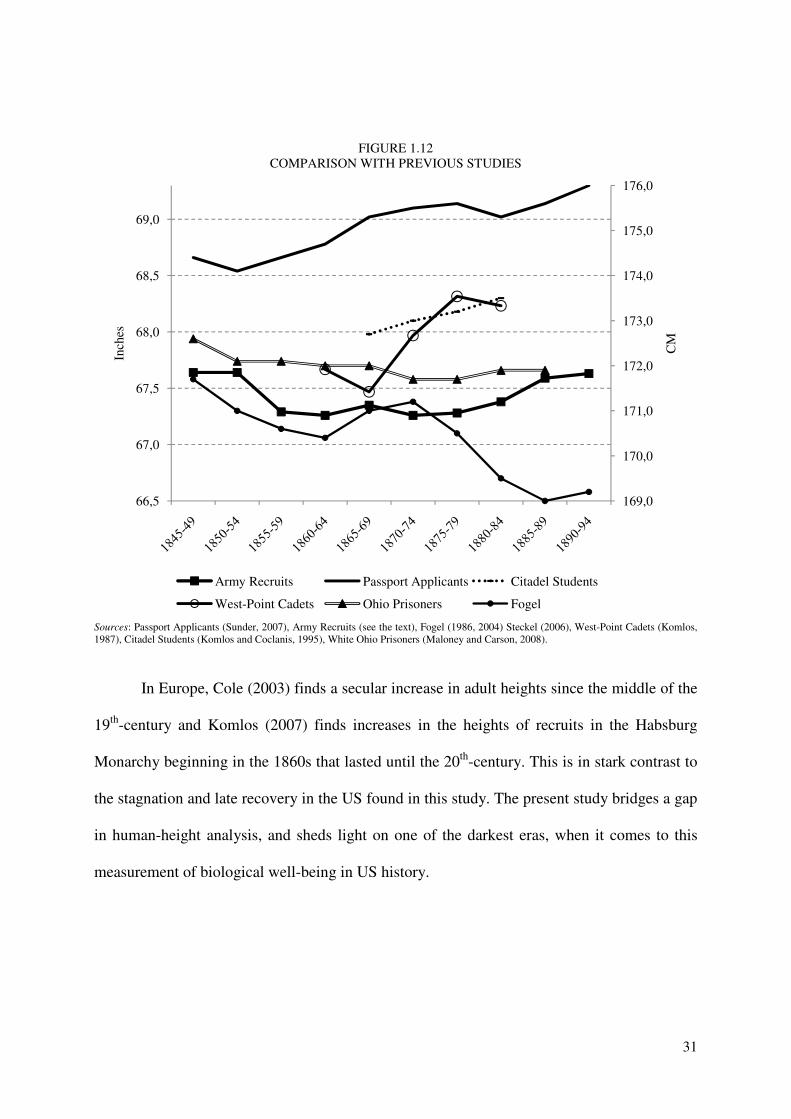
1875. The difference is substantial: by 1890 it is 1.02 inches (2.6 cm). Figure 1.12 compares

our findings with other studies of this time period.

168,0

169,0

170,0

171,0

172,0

173,0

174,0

66,1

66,6

67,1

67,6

68,1

CM

Inch

es

Army Army Constrained Ohio National Guard Fogel

31

FIGURE 1.12 COMPARISON WITH PREVIOUS STUDIES

Sources: Passport Applicants (Sunder, 2007), Army Recruits (see the text), Fogel (1986, 2004) Steckel (2006), West-Point Cadets (Komlos, 1987), Citadel Students (Komlos and Coclanis, 1995), White Ohio Prisoners (Maloney and Carson, 2008).

In Europe, Cole (2003) finds a secular increase in adult heights since the middle of the

19th-century and Komlos (2007) finds increases in the heights of recruits in the Habsburg

Monarchy beginning in the 1860s that lasted until the 20th-century. This is in stark contrast to

the stagnation and late recovery in the US found in this study. The present study bridges a gap

in human-height analysis, and sheds light on one of the darkest eras, when it comes to this

measurement of biological well-being in US history.

169,0

170,0

171,0

172,0

173,0

174,0

175,0

176,0

66,5

67,0

67,5

68,0

68,5

69,0

CM

Inch

es

Army Recruits Passport Applicants Citadel Students

West-Point Cadets Ohio Prisoners Fogel

32

1.3.2 County and State Level Determinants of Height

We include county-level variables in order to test how urbanization, the availability of

nutrients, wages, transportation, geographic mobility, and the epidemiological framework

affected stature as in Craig and Weiss (1998), Haines, Craig, and Weiss (2003), and Sunder

(2007). The sample is reduced to 41,830 recruits because 16,682 recruits could not be

assigned to their counties of birth. For state-level data the sample is further reduced to 41,713

because data on infant mortality and the railroad network were not available for all states.

We begin by examining the hypothesis that population density affected exposure to

diseases and nutrition, and consequently height. During the period of US history under

consideration, urban food prices were more expensive than in rural areas, because of

transportation costs, and of inferior quality, because of deterioration in the course of

transportation (refrigeration was just beginning) (Komlos, 1987, 2003; Craig, Goodwin, and

Grennes, 2004). Furthermore, poor sanitation, a large immigrant population, and overcrowded

living conditions facilitated the transmission of diseases, and thereby stunted growth (Preston

and Haines, 1991; Steckel, 1995; Lee, 1997; Craig and Weiss, 1998; Haines, Craig, and

Weiss, 2003). In order to distinguish varying degrees of urbanization, three census categories

are adopted5. The reference category is “rural,” that is, agglomerations of no more than 2,500

inhabitants. The other categories are towns with populations between 2,500 and 25,000 and

urban areas with more than 25,000 inhabitants.

The agricultural-output variables reflect the local availability of nutrients. For

instance, those living in counties with dairy and livestock operations faced lower prices for

these products insofar as they did not have to pay transportation costs or for the profits of

middlemen. As a consequence they would consume more calcium and protein and thereby

5 The categories measure the proportion of county inhabitants in each group.

33

grow taller than those less fortunate in their location: thus one can infer that there should be a

height premium for nutrient propinquity. Indeed many studies have documented such a

premium (Komlos, 1987; Craig and Weiss, 1998; Haines, Craig, and Weiss, 2003). Because

milk could not be transported over long distances, milk cows per capita influenced height

locally (Baten, 1999). Since butter and cheese, unlike milk, could be shipped, dairy farmers

near cities supplied those cities with milk, whereas dairy farmers in more remote areas

produced butter and cheese. Beginning in the 1870s, improvements in transportation and

refrigeration meant that milk could be transported over longer distances (Bateman, 1968). The

meat industry, too, was transformed by these improvements. Dressed beef could be

transported; previously, livestock had to be transported close to the market in question and

only then slaughtered and dressed (Yeager Kujovich, 1970). Hence, market integration, which

in turn depended upon good transportation networks, was important for nutritional status. In

other words, height is in part a function of nutrient availability, which is in part a function

both of its distribution and of market integration. Equal distribution and easy access to locally

produced nutrients would have a positive effect on local height. Market integration, made

possible by improvements in transportation, would affect the height of agricultural

populations because nutrients would be shipped to distant markets rather than consumed

locally.

The nominal annual wage per manufacturing worker is the best proxy available for

non-farm incomes in the census at the county level. Higher income was accompanied by

higher meat consumption, and animal protein promotes growth (Cuff, 2005). Furthermore, a

rise in income permits a move to better housing, which is associated with a decline in illness

and in infant mortality (Preston and Haines, 1991). Categories for civilian occupations were

included to control for the socio-economic background of the recruits. A simplifying

assumption is that there was little intergenerational mobility: a recruit’s occupation prior to

34

joining the service is a valid predictor of his parent's occupations6. These occupations were

coded into the following categories: farmers, laborers (including those temporarily

unemployed or with no reported occupation), lower-level white-collar workers, upper-level

white-collar workers, semi-skilled blue-collar workers, and skilled blue-collar workers.

Recruits from higher socio-economic strata are expected to be taller than the others, in line

with findings by Komlos (1987), Steckel (1995), Sunder (2007), and Hiermeyer (2008).

Higher socio-economic status would have a positive effect on stature; well-to-do families

could afford more and better quality food and better housing (Preston and Haines, 1991). On

the other hand, it is possible that those who were taller and healthier than average were also

more productive and therefore had better-paying jobs in adulthood, so the direction of the

causality is not clear (Lee, 1997). A recruit who enlisted out of state is classified as a mover.

There are two hypotheses regarding movers: that they were mostly poor and malnourished

(and therefore shorter than average), and moved to another state in the hope of improving

their lot; or that moving was costly and therefore movers were also well-nourished (and taller

than average) (Craig and Weiss, 1998; Haines, Craig, and Weiss, 2003).

Data for transportation and the disease environment, both important variables, cannot

be analyzed at the county level because there are no such data in the 1880 census. We remedy

this problem by supplementing this analysis with variables aggregated at the state-level. State

infant mortality rates7 serve as a proxy variable for the disease environment. The effect of

infant mortality on height is expected to be negative through the channel of diseases because

energy normally channeled into growth is lost to the fight against diseases (Preston and

Haines, 1991). The length of railroad lines completed in a state as of June 30, 1880 (measured

in 1,000 miles) is used as a proxy for access to transportation. Transportation promotes access

6 For an analysis of this assumption see Chapter 3.

7 The number of deaths of infants - that is, children under the age of 1 year -per 1000 births.

35

not only to markets but also to diseases, so its effect on (rural) height should be negative

(Sunder, 2007). Market integration could either lead to a better and more balanced diet,

promoting growth because healthy food would become more available and affordable

especially in cities, or it could lead to a substitution away from protein- and calcium-rich

foods to a carbohydrate-based diet especially for nutrient exporting regions (Komlos, 1987,

1996). To test these hypotheses we estimate regressions on the national and regional level

with county-level data (Tables 1.10 and 1.11) and on the national level with county- and state-

level data (Table 1.12).

Results from Table 1.10 confirm that the proportion of a given county population

living in towns with more than 2,500 inhabitants was negatively correlated with adult height,

which is significant only in Model 3 (a ten percentage point increase in the county share of

those living in towns was associated with 0.02 in. / 0.1 cm lower heights). However, in all

models the proportion of people living in urban areas with more than 25,000 people was

negatively associated with stature of almost twice the magnitude of the town category (here a

ten percentage point increase in the county share of those living in cities was associated with

0.04 in. / 0.1 cm lower heights). In other words, a high population density brought about by

urbanization was correlated with short stature.

Milk cows and pigs per capita were significantly and positively correlated with height

confirming the propinquity thesis, whereas wheat per capita and height were not significantly

correlated8 (Table 1.10). Although grain provides energy, in the form of carbohydrates, it

contains much less calcium and protein than meat, essential for growth (Waterlow, 1994).

8 See Baten’s (1999) finding that in Bavaria between 1730 and 1880 recruits from wheat-producing regions were shorter than

those from dairy regions.

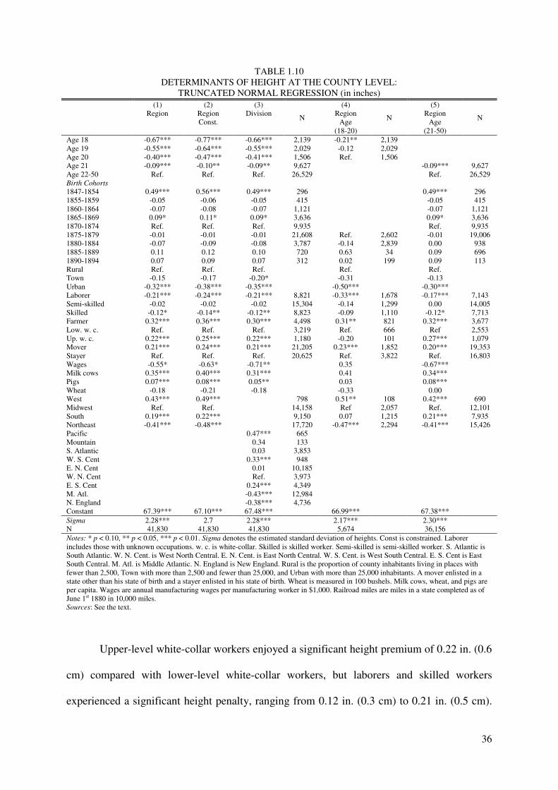
36

TABLE 1.10 DETERMINANTS OF HEIGHT AT THE COUNTY LEVEL:

TRUNCATED NORMAL REGRESSION (in inches)

(1) Region

(2) Region Const.

(3) Division

N

(4) Region

Age (18-20)

N

(5) Region

Age (21-50)

N

Age 18 -0.67*** -0.77*** -0.66*** 2,139 -0.21** 2,139 Age 19 -0.55*** -0.64*** -0.55*** 2,029 -0.12 2,029 Age 20 -0.40*** -0.47*** -0.41*** 1,506 Ref. 1,506 Age 21 -0.09*** -0.10** -0.09** 9,627 -0.09*** 9,627 Age 22-50 Ref. Ref. Ref. 26,529 Ref. 26,529 Birth Cohorts 1847-1854 0.49*** 0.56*** 0.49*** 296 0.49*** 296 1855-1859 -0.05 -0.06 -0.05 415 -0.05 415 1860-1864 -0.07 -0.08 -0.07 1,121 -0.07 1,121 1865-1869 0.09* 0.11* 0.09* 3,636 0.09* 3,636 1870-1874 Ref. Ref. Ref. 9,935 Ref. 9,935 1875-1879 -0.01 -0.01 -0.01 21,608 Ref. 2,602 -0.01 19,006 1880-1884 -0.07 -0.09 -0.08 3,787 -0.14 2,839 0.00 938 1885-1889 0.11 0.12 0.10 720 0.63 34 0.09 696 1890-1894 0.07 0.09 0.07 312 0.02 199 0.09 113 Rural Ref. Ref. Ref. Ref. Ref. Town -0.15 -0.17 -0.20* -0.31 -0.13 Urban -0.32*** -0.38*** -0.35*** -0.50*** -0.30*** Laborer -0.21*** -0.24*** -0.21*** 8,821 -0.33*** 1,678 -0.17*** 7,143 Semi-skilled -0.02 -0.02 -0.02 15,304 -0.14 1,299 0.00 14,005 Skilled -0.12* -0.14** -0.12** 8,823 -0.09 1,110 -0.12* 7,713 Farmer 0.32*** 0.36*** 0.30*** 4,498 0.31** 821 0.32*** 3,677 Low. w. c. Ref. Ref. Ref. 3,219 Ref. 666 Ref 2,553 Up. w. c. 0.22*** 0.25*** 0.22*** 1,180 -0.20 101 0.27*** 1,079 Mover 0.21*** 0.24*** 0.21*** 21,205 0.23*** 1,852 0.20*** 19,353 Stayer Ref. Ref. Ref. 20,625 Ref. 3,822 Ref. 16,803 Wages -0.55* -0.63* -0.71** 0.35 -0.67*** Milk cows 0.35*** 0.40*** 0.31*** 0.41 0.34*** Pigs 0.07*** 0.08*** 0.05** 0.03 0.08*** Wheat -0.18 -0.21 -0.18 -0.33 0.00 West 0.43*** 0.49*** 798 0.51** 108 0.42*** 690 Midwest Ref. Ref. 14,158 Ref 2,057 Ref. 12,101 South 0.19*** 0.22*** 9,150 0.07 1,215 0.21*** 7,935 Northeast -0.41*** -0.48*** 17,720 -0.47*** 2,294 -0.41*** 15,426 Pacific 0.47*** 665 Mountain 0.34 133 S. Atlantic 0.03 3,853 W. S. Cent 0.33*** 948 E. N. Cent 0.01 10,185 W. N. Cent Ref. 3,973 E. S. Cent 0.24*** 4,349 M. Atl. -0.43*** 12,984 N. England -0.38*** 4,736 Constant 67.39*** 67.10*** 67.48*** 66.99*** 67.38*** Sigma 2.28*** 2.7 2.28*** 2.17*** 2.30*** N 41,830 41,830 41,830 5,674 36,156 Notes: * p < 0.10, ** p < 0.05, *** p < 0.01. Sigma denotes the estimated standard deviation of heights. Const is constrained. Laborer includes those with unknown occupations. w. c. is white-collar. Skilled is skilled worker. Semi-skilled is semi-skilled worker. S. Atlantic is South Atlantic. W. N. Cent. is West North Central. E. N. Cent. is East North Central. W. S. Cent. is West South Central. E. S. Cent is East South Central. M. Atl. is Middle Atlantic. N. England is New England. Rural is the proportion of county inhabitants living in places with fewer than 2,500, Town with more than 2,500 and fewer than 25,000, and Urban with more than 25,000 inhabitants. A mover enlisted in a state other than his state of birth and a stayer enlisted in his state of birth. Wheat is measured in 100 bushels. Milk cows, wheat, and pigs are per capita. Wages are annual manufacturing wages per manufacturing worker in $1,000. Railroad miles are miles in a state completed as of June 1st 1880 in 10,000 miles. Sources: See the text.

Upper-level white-collar workers enjoyed a significant height premium of 0.22 in. (0.6

cm) compared with lower-level white-collar workers, but laborers and skilled workers

experienced a significant height penalty, ranging from 0.12 in. (0.3 cm) to 0.21 in. (0.5 cm).

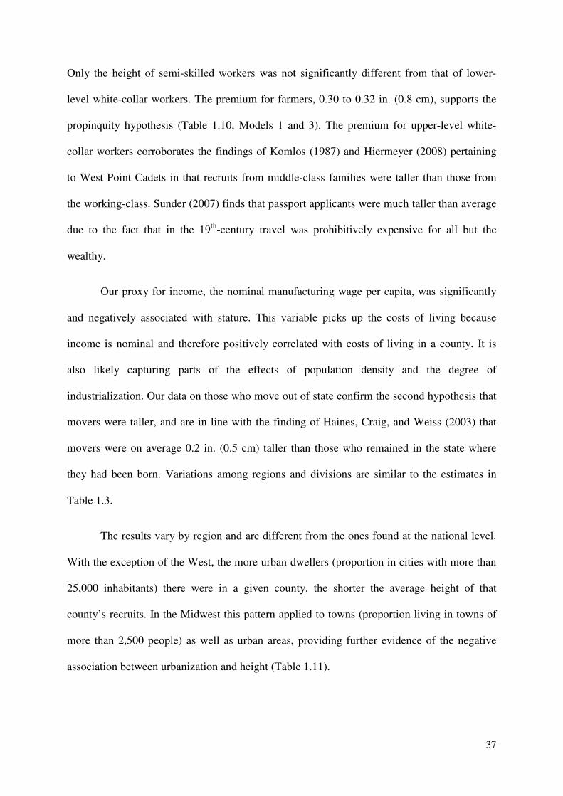
37

Only the height of semi-skilled workers was not significantly different from that of lower-

level white-collar workers. The premium for farmers, 0.30 to 0.32 in. (0.8 cm), supports the

propinquity hypothesis (Table 1.10, Models 1 and 3). The premium for upper-level white-

collar workers corroborates the findings of Komlos (1987) and Hiermeyer (2008) pertaining

to West Point Cadets in that recruits from middle-class families were taller than those from

the working-class. Sunder (2007) finds that passport applicants were much taller than average

due to the fact that in the 19th-century travel was prohibitively expensive for all but the

wealthy.

Our proxy for income, the nominal manufacturing wage per capita, was significantly

and negatively associated with stature. This variable picks up the costs of living because

income is nominal and therefore positively correlated with costs of living in a county. It is

also likely capturing parts of the effects of population density and the degree of

industrialization. Our data on those who move out of state confirm the second hypothesis that

movers were taller, and are in line with the finding of Haines, Craig, and Weiss (2003) that

movers were on average 0.2 in. (0.5 cm) taller than those who remained in the state where

they had been born. Variations among regions and divisions are similar to the estimates in

Table 1.3.

The results vary by region and are different from the ones found at the national level.

With the exception of the West, the more urban dwellers (proportion in cities with more than

25,000 inhabitants) there were in a given county, the shorter the average height of that

county’s recruits. In the Midwest this pattern applied to towns (proportion living in towns of

more than 2,500 people) as well as urban areas, providing further evidence of the negative

association between urbanization and height (Table 1.11).

38

TABLE 1.11 DETERMINANTS OF HEIGHT AT THE COUNTY LEVEL BY CENSUS REGION:

TRUNCATED NORMAL REGRESSION (in inches) (1)

West N

(2) Midwest

N (3)

South N

(4) Northeast

N

Age 18 -0.86 38 -0.52*** 830 -0.85*** 409 -0.68*** 862 Age 19 -0.18 40 -0.42*** 673 -0.63*** 463 -0.64*** 853 Age 20 -0.14 30 -0.38** 554 -0.53*** 343 -0.35** 579 Age 21 0.33 180 -0.01 3,415 -0.15* 2,042 -0.15* 3,989 Age 22-50 Ref. 510 Ref. 8,686 Ref. 5,893 Ref. 11,437 Birth Cohorts 1847-1864 0.63 22 1865-1879 Ref. 726 1880-1894 0.68 50 1847-1854 0.26 64 0.29 77 0.81*** 155 1855-1859 -0.26 101 0.05 112 0.03 200 1860-1864 0.03 354 0.00 254 -0.17 493 1865-1869 0.17* 1,215 0.02 796 -0.11 1,554 1870-1874 Ref. 3,225 Ref. 2,226 Ref. 4,270 1875-1879 0.02 7,429 0.00 4,745 -0.02 8,990 1880-1884 -0.13 1,430 -0.11 730 -0.06 1,587 1885-1889 0.25 251 0.04 136 0.03 325 1890-1894 0.33 89 -0.01 74 -0.04 146 Rural Ref. Ref. Ref. Ref. Town -0.52 -0.42* -0.50 -0.11 Urban -0.37 -0.54*** -0.32 -0.62*** Laborer 0.62* 130 -0.08 2,857 -0.11 1,997 -0.40*** 3,835 Semi-skilled 0.16 292 0.07 4,652 0.26* 3,285 -0.23** 7,075 Skilled 0.29 171 -0.05 2,894 0.19 1,394 -0.35*** 4,364 Farmer 0.79 40 0.27** 2,179 0.59*** 1,643 0.05 636 Low. w. c. Ref. 134 Ref. 1,151 Ref. 563 Ref. 1,370 Up. w. c. 1.57*** 32 0.17 427 0.33 271 0.09 449 Mover 0.22 313 0.18*** 7,701 0.12* 5,187 0.21*** 8,001 Stayer Ref. 485 Ref. 6,457 Ref. 3,963 Ref. 9,719 Wages -0.11 -0.10* -0.26 1.40** Milk cows p.c. -0.10 -0.05 0.30 0.56** Pigs p.c. 0.39 0.03 0.08 -0.22 Wheat p.c. 0.30 -0.54*** -1.00* -0.01 Mountain 0.06 133 Pacific Ref. 665 Iowa -0.32 813 Nebraska -0.14 167 MN,SD,ND Ref. 373 Kansas -0.10 551 Missouri -0.56*** 2,069 Wisconsin -0.18 495 Michigan -0.61*** 1,162 Illinois -0.39** 2,244 Indiana -0.26 2,373 Ohio -0.51*** 3,911 OK,AR 0.68** 206 Texas 1.15*** 569 Louisiana 0.82*** 173 Kentucky 0.84*** 2,458 Tennessee 1.01*** 1,242 Mississippi 1.04*** 185 Alabama 0.93*** 464 West Virginia 0.93*** 304 Virginia 0.90*** 780 Delaware -0.04 103 North Carolina 1.11*** 571 South Carolina 0.86*** 381 DC, Maryland Ref. 776 Georgia 0.85*** 875 Florida 0.47 63 New York 0.04 6,238 Pennsylvania Ref. 5,455 Vermont -0.06 227 New Hampshire -0.28 176 Massachusetts -0.04 2,823 Connecticut -0.15 638 Rhode Island 0.13 456 Maine 0.23 416 New Jersey -0.02 1,291 Constant 67.05*** 68.14*** 66.61*** 66.62*** Sigma 2.14*** 2.26*** 2.27*** 2.30***

39

TABLE 1.11 CONTINUED N 798 14,158 9,150 17,720 Notes: * p < 0.10, ** p < 0.05, *** p < 0.01. Sigma denotes the estimated standard deviation of heights. Laborer includes those with unknown occupations. w. c. is white-collar. Skilled is skilled worker. Semi-skilled is semi-skilled worker. Rural is the proportion of county inhabitants living in places with fewer than 2,500, Town with more than 2,500 and fewer than 25,000, and Urban with more than 25,000 inhabitants. A mover enlisted in a state other than his state of birth and a stayer enlisted in his state of birth. Wheat is measured in 100 bushels. p.c. is per capita. Wages are annual manufacturing wages per manufacturing worker in $1,000. MN= Minnesota. SD=South Dakota. ND=North Dakota. OK=Oklahoma. AR=Arkansas. Sources: See the text.

The average height within a given occupation differed from region to region. While

farmers and upper-level white-collar workers were significantly taller in the nationwide

regression, farmers were only significantly taller in the South and Midwest and upper-level

white-collar workers only in the West. In the South semi-skilled workers were significantly

taller, while they were significantly shorter in the Northeast. Skilled workers suffered from a

height penalty in the nationwide regression, yet there was no significant effect on the regional

level. Laborers, significantly shorter at the national level, were significantly taller than lower-

level white-collar workers in the West, yet shorter in the Northeast. With the exception of the

West, those recruits who enlisted in a state other than the one in which they were born had a

significant height advantage (Table 1.11).

The aggregate variables at the regional level differ somewhat from those at the

national level. It is only in the Northeast that milk cows per capita and height were

significantly and positively correlated, whereas pigs per capita were not significantly

correlated, and it is only in the Midwest and the South that the correlation of wheat production

was significant and negative. In the Northeast the annual manufacturing wage per capita was

significant and positive, whereas it was significant and negative in the Midwest and in the

nationwide regression (Table 1.11).

40

TABLE 1.12 DETERMINANTS OF HEIGHT AT THE STATE AND COUNTY LEVEL:

TRUNCATED NORMAL REGRESSION (in inches) (1)

Region Age

(18-50)

(2) Region

Constrained Age (18-50)

(3) Division

Age (18-50)

N

(4) Region

Age (18-20)

N

(5) Region

Age (21-50)

N

Age 18 -0.67*** -0.77*** -0.66*** 2,133 -0.21** 2,133 Age 19 -0.55*** -0.64*** -0.55*** 2,026 -0.12 2,026 Age 20 -0.40*** -0.46*** -0.40*** 1,498 Ref. 1,498 Age 21 -0.09** -0.11** -0.09** 9,589 -0.09** 9,589 Age 22-50 Ref. Ref. Ref. 26,467 Ref. 26,467

Birth Cohorts 1847-1854 0.49*** 0.56*** 0.49*** 296 0.49*** 296 1855-1859 -0.04 -0.05 -0.04 414 -0.04 414 1860-1864 -0.07 -0.08 -0.07 1,121 -0.07 1,121 1865-1869 0.09* 0.10* 0.09* 3,630 0.09* 3,630 1870-1874 Ref. Ref. Ref. 9,914 Ref. 9,914

1875-1879 -0.01 -0.01 -0.01 21,528 0.14* 2,592 -0.01 18,936 1880-1884 -0.08 -0.09 -0.08 3,779 Ref 2,832 -0.01 937 1885-1889 0.11 0.13 0.11 719 0.76* 34 0.10 695 1890-1894 0.07 0.09 0.08 312 0.16 199 0.09 113 Rural Ref. Ref. Ref. Ref. Ref. Town -0.17 -0.19 -0.21* -0.27 -0.15 Urban -0.31*** -0.37*** -0.34*** -0.47** -0.29***

Infant mortality -0.02** -0.02*** -0.02*** -0.02 -0.02*** Laborer -0.22*** -0.25*** -0.22*** 8,796 -0.35*** 1,674 -0.18*** 7,122 Semi-skilled -0.02 -0.03 -0.02 15,262 -0.16 1,295 0.00 13,967 Skilled -0.12** -0.14** -0.12** 8,805 -0.10 1,108 -0.11* 7,697 Farmer 0.31*** 0.36*** 0.30*** 4,490 0.30* 820 0.32*** 3,670 Lower w. collar Ref. Ref. Ref. 3,199 Ref. 660 Ref. 2,539

Upper w. collar 0.22*** 0.25** 0.22*** 1,176 -0.22 101 0.27*** 1,075 Mover 0.20*** 0.23*** 0.21*** 21,118 0.23*** 1,840 0.19*** 16,778 Stayer Ref. Ref. Ref. 20,595 Ref. 3,817 Ref. 19,278 Wages -0.52** -0.59** -0.68*** 0.28 -0.63** Milk cows p.c. 0.36*** 0.41*** 0.32*** 0.45 0.34*** Pigs p.c. 0.07*** 0.08*** 0.05** 0.03 0.08***

Railroad miles 0.00 0.00 0.00 0.00 0.00 Wheat p.c. -0.19 -0.22 -0.19 -0.29 -0.18 West 0.38*** 0.44** 707 0.60* 94 0.35*** 613 Midwest Ref. Ref. 14,136 Ref. 2,054 Ref. 12,082 South 0.17*** 0.19*** 9,150 0.10 1,215 0.18*** 7,935 Northeast -0.38*** -0.44*** 17,720 -0.42*** 2,294 -0.37*** 15,426

Pacific 0.44*** 649 Mountain 0.26 58 South Atlantic 0.04 3,853 West South C. 0.32*** 948 East North C. -0.01 10,185 West North C. Ref. 3,951 East South C. 0.24*** 4,349

Middle Atlantic -0.41*** 12,984 New England -0.34*** 4,736 Constant 67.61*** 67.36*** 67.63*** 66.98*** 67.62***

Sigma 2.28*** 2.70 2.28*** 2.17*** 2.30*** N 41,713 41,713 41,713 5,657 36,056

Notes: * p < 0.10, ** p < 0.05, *** p < 0.01. Sigma denotes the estimated standard deviation of heights. Constrained estimates are estimated with the standard deviation set to 2.7 in. (6.86 cm). Laborer includes those with unknown occupations. w. collar = white-collar. Skilled is skilled worker. Semi-skilled is semi-skilled worker. North C. = North Central, South C. =South Central. Rural is the proportion of county inhabitants living in places with fewer than 2,500, Town with more than 2,500 and fewer than 25,000, and Urban with more than 25,000 inhabitants. A mover enlisted in a state other than his state of birth and a stayer enlisted in his state of birth. Wheat is measured in 100 bushels. p.c. is per capita. Wages are annual manufacturing wages per manufacturing worker in $1,000. Infant mortality is measured in deaths per 1,000 births. Railroad miles are miles in a state completed as of June 1st 1880 in 10,000 miles. Sources: See the text.

41

The state infant-mortality rates were significantly and negatively associated with

stature, confirming the hypothesis that the above-average disease rate in an unhealthy

environment that accounted for an above-average infant-mortality rate also accounted for

below-average adult heights (Table 1.12). There was no significant correlation between the

number of miles of state rail lines and average height, even though railroads facilitated the

spread of disease and the trading away of growth-enhancing nutrients. A valid explanation

could be technical: that the high level of aggregation fails to capture the county-by-county

variation in railroad access. The results from Table 1.10 are robust to the inclusion of state

level data (Table 1.12).

1.4 Conclusion

This study of the physical stature of US-born recruits into the Federal Army for the birth

cohorts circa 1850-1890 fills a lacuna in the literature. The anthropometric studies that were

done on this period tended to be either regionally limited (Ohio, South Carolina) or were

limited to the elite segment of the population (West Point Cadets, passport applicants). This is

the first study of a national data set based on a large sample of US Army recruits. In addition

to estimating the trend for the nation as a whole in this period, the study also examines how

and to what degree local nutrients, urbanization, market integration, occupations, and a

disease-prone environment affected stature.

This study finds that the decline in physical stature that began in the 1830s continued

into the 1850s. The decline in the 1850s was about 0.4 in. (1.0 cm) from 67.64 in. (171.8 cm)

in the early 1850s birth cohort to a nadir of 67.26 in. (170.8 cm) in the cohort born during the

Civil War and heights remained virtually unchanged until the 1880s, when they started to

increase.

42

Average regional heights ranged from a high of 67.69 in. (171.9 cm) in the South to a

low of 66.67 in. (169.3 cm) in the Northeast. Despite the Civil War the South was consistently

the tallest region, with no significant changes in stature between the early 1850s and the late

1870s, while the Northeast remained the shortest region just like before the war.

We find that protein and calcium availability were significantly and positively

correlated with height both at the national level and in the Northeast similar to findings by

Craig and Weiss (1998). The correlation with urbanization (towns as well as cities) was

significant and negative both at the national level (controlling for divisions) and in the

Midwest and South at the regional level. Infant mortality, used as an indicator for the disease

environment, was significantly and negatively associated with height. As for height

differences according to occupation, the tallest were upper-level white-collar workers, who

could afford better than average food and housing, and farmers, who enjoyed lower relative

prices and greater than average proximity to food sources (Komlos, 1987; Lee, 1997)

While this study confirms the conclusions of previous studies concerning the effect of

certain established variables on height, it also reveals considerable regional variability. The

rapid economic growth that accompanied urbanization, industrialization, and market

integration brought 19th-century America many benefits, but they came at a high price: the

stagnation in height that translates as stagnation in biological well-being. This study puts the

national trend in height on a solid evidential basis. So far trends have mostly been based on

extrapolation of local trends derived from Ohio. Our findings show that heights stagnated for

a generation after the Civil War in spite of the substantial economic growth especially in the

North and the West. Not until the birth cohorts of the 1890s did the benefits of economic

growth filter down to affect the biological standard of living of the common people. In

contrast, the height of the elite, both men and women, were increasing rapidly beginning with

the 1850s. Hence, quite a considerable gulf developed between the common man and the elite

43

segments of the society: In 1850 passport applicants were 0.91 in. (2.3 cm) taller than Army

recruits and in 1890 the gap had widened to 1.65 in. (4.2 cm). In 1890 the common man had

reached the 1850 level again after decades of stagnation, while the elite continually grew.

44

References

Data:

Minnesota Population Center. 2004. National Historical Geographic Information System

(NHGIS): Pre-release Version 0.1. Minneapolis, MN: University of Minnesota.

http://www.nhgis.org

National Archives and Records Administration. 7th and Pennsylvania Ave., NW

Washington DC 20408-0001. Microfilm ID M233. Record Group 094. Register of

Enlistments in the U.S. Army, 1798-1914. Vol 94 (96%), Vol 96 (100%), Vol 97(10%), Vol

98 (93%), Vol 100 (88%),Vol 102 (100%), Vol 103 (80%), Vol 104 (100%), Vol 105 (100%).

Literature:

A’Hearn, Brian. 1998. “The Antebellum Puzzle Revisited: A New Look at the Physical

Stature of Union Army Recruits during the Civil War.” In: The Biological Standard of Living

in Comparative Perspective, ed. John Komlos and Joerg Baten, 250-267. Stuttgart: Franz

Steiner.

A’Hearn, Brian. 2004. “A restricted maximum likelihood estimator for truncated height

samples.” Economics and Human Biology, 2: 5-19.

Bateman, Fred. 1968. “Improvement in American Dairy Farming, 1850-1910: A

Quantitative Analysis.” The Journal of Economic History, 28: 255-273.

Baten, Jörg. 1999. “Ernährung und wirtschaftliche Entwicklung in Bayern (1730-

1880).” In: Beiträge zur Wirtschafts-und Sozialgeschichte. Stuttgart: Steiner Verlag.

Bogin, Barry. 1999. Patterns of Human Growth. Cambridge: Cambridge University Press.

Cole, T. J. 2000. “Galton’s midparent height revisited.” Annals of Human Biology, 27 (4):

401-405.

Cole, T. J. 2003. “The secular trend in human physical growth: a biological view.”

Economics and Human Biology, 1: 161-168.

Craig, Lee A., and Thomas Weiss. 1998. “Nutritional Status and Agricultural Surpluses in

the Antebellum United States.” In: The Biological Standard of Living in Comparative

Perspective, ed. John Komlos and Joerg Baten, 190-207. Stuttgart: Franz Steiner.

Craig, Lee A., Barry Goodwin, and Thomas Grennes. 2004. “The Effect of Mechanical

Refrigeration on Nutrition in the United States.” Social Science History, 28: 325-336

Cuff, Timothy. 2005. The Hidden Cost of Economic Development. The Biological Standard

of Living in Antebellum Pennsylvania. Hampshire, UK: Ashgate.

45

Davis, George B. 1898. The Military Laws of the United States. Washington, D.C.:

Government Printing Office.

Crawford, Michael J., Mark L. Hayes, and Michael D. Sessions. 1998. “The Spanish-

American War: historical overview and select bibliography.” Naval History Bibliographies;

no. 5. Washington DC: Government Printing Office.

Davis, Joseph H. 2004. “An Annual Index of U.S. Industrial Production, 1790-1915.”

Quarterly Journal of Economics, 119: 1177-1215.

Fogel, Robert. 1986. “Nutrition and the Decline in Mortality: Some Preliminary Findings.”

In: Long-Term Factors in American Economic Growth, 439-555. Chicago: University of

Chicago Press (for NBER).

Fogel, Robert. 1994. “Economic Growth, Population Theory, and Physiology: the Bearing of

Long-term Processes on the Making of Economic Policy.” American Economic Review, 84:

369–395.

Fogel, Robert. 2004. The Escape from Hunger and Premature Death, 1700-2100 Europe,

America, and the Third World. Cambridge: Cambridge University Press.

Frisancho, Robert. A. 1990. Anthropometric Standards for the Assessment of Growth and

Nutritional Status. Ann Arbor: University of Michigan Press.

Gallman, Robert E. 1960. “Commodity Output, 1839-1899.” In: Trends in the American

Economy in the Nineteenth Century, Studies in Income and Wealth Vol. 24, ed. William N.

Parker, 13-72. Princeton: Princeton University Press.

Gallman, Robert E.1966. ”Gross National Product in the United States, 1834-1909.” In:

Output, Employment, and Productivity in the United States after 1800, Studies in Income and

Wealth Vol. 30, ed. Dorothy S. Brady,1-90. New York: Columbia University Press.

Gallman, Robert E. 2000. “Economic Growth and Structural Change in the Long Nineteenth

Century,” In: Cambridge Economic History of the United States, Vol. II, ed. Stanley

Engerman and Robert E. Gallman, 1-56. Cambridge: Cambridge University Press.

Haines, Michael, Lee A. Craig, and Thomas Weiss. 2003. “The Short and the Dead:

Nutrition, Mortality, and the ‘Antebellum Puzzle’ in the United States.” Journal of Economic

History, 63: 382-413.

Hiermeyer, Martin. 2008. “Four Empirical Essays on the Economics of Height.” PhD diss.

University of Munich.

Hughes, Jonathan, and Louis P. Cain. 2002. American Economic History. 6th ed. New

York: Addison-Wesley.

Johnston, Louis D., and Samuel H. Williamson. 2008. “What Was the U.S. GDP Then?”

Measuring Worth. http://www.measuringworth.org/usgdp/ (accessed September 27, 2009).

46

Komlos, John. 1987. “The Height and Weight of West Point Cadets: Dietary Change in

Antebellum America.” The Journal of Economic History, 47: 897-927.

Komlos, John. 1996. “Anomalies in economic history: Reflections on the antebellum

puzzle.” Journal of Economic History, 56: 202-214.

Komlos, John. 2003. “Access to Food and the Biological Standard of Living: Perspectives on

the Nutritional Status of Native Americans.” American Economic Review, 93: 252-255.

Komlos, John. 2004a. “Improvements in Maximum Likelihood Estimators of Truncated

Normal Samples with Prior Knowledge of σ. A Simulation Based Study with Application to

Historical Height Samples.” Discussion Paper LMU Munich.

Komlos, John. 2004b. “How to (and How Not to) Analyze Deficient Height Samples.”

Historical Methods, 37 (4): 160-173.

Komlos, John. 2007. “Anthropometric evidence on economic growth, biological well-being

and regional convergence in the Habsburg Monarchy, c. 1850-1910.” Cliometrica, 1: 211-

237.

Komlos, John, and Peter A. Coclanis. 1995. “Nutrition and Economic Development in Post-

Reconstruction South Carolina: An Anthropometric Approach.” Social Science History, 19

(1): 91-115.

Lee, Chulhee. 1997. “Socioeconomic Background, Disease, and Mortality among Union

Army Recruits: Implications for Economic and Demographic History.” Explorations in

Economic History, 34: 27-55.

Maloney, Thomas N., and Scott Alan Carson. 2008. “Living Standards in Black and White:

Evidence from the heights of Ohio Prison Inmates, 1829-1913.”.Economics and Human

Biology, (6): 237-251.

Margo, Robert, and Richard Steckel. 1983. “Heights of Native Born Northern Whites

during the Antebellum Period.” Journal of Economic History, 43: 167-184.

Preston, Samuel H., and Michael Haines. 1991. Fatal Years: Child Mortality in the Late

Nineteenth-Century America. Princeton, NJ: Princeton University Press.

Rhode, Paul W. 2002. Gallman’s Annual Output Series for the United States, 1834-1909.

NBER Working Paper No. W8860.

Sellers, James L. 1927. “The Economic Incidence of the Civil War in the South.” The

Mississippi Valley Historical Review, 14 (2): 179-191.

Smith, Joseph. 1994. The Spanish-American War: Conflict in the Caribbean and the Pacific

1895-1902. Singapore: Longman.

47

Steckel, Richard, and Donald Haurin. 1994. “Health and Nutrition in the American

Midwest: Evidence from the Height of Ohio National Guardsmen, 1850-1910.” In: Stature,

Living Standards, and Economic Development: Essays in Anthropometric History, ed. John

Komlos, 117-128. Chicago: The University of Chicago Press.

Steckel, Richard. 1995. “Stature and the Standard of Living.” Journal of Economic

Literature, 33 (4): 1903-1940.

Steckel, Richard. 2006. “Health, Nutrition and Physical Well-Being” In: Historical Statistics

of the United States, Earliest Times to the Present: Millennial Edition, ed. Susan B. Carter,

Scott Sigmund Gartner, Michael R. Haines, Alan L. Olmstead, Richard Sutch, and Gavin

Wright. Bd 653-654. New York: Cambridge University Press.

Sunder, Marco. 2007. “Passports and Economic Development: An Anthropometric History

of the U.S. Elite in the Nineteenth Century.” PhD diss. University of Munich.

Tanner, James M. 1978. Foetus into Man: Physical Growth from Conception to Maturity.

Cambridge: Cambridge University Press.

U.S. Census Bureau. 2002. Geography Division.

http://www.census.gov/geo/www/us_regdiv.pdf (accessed December 2009).

Waterlow, John. 1994. “Summary of Causes and Mechanisms of Linear Growth

Retardation.” European Journal of Clinical Nutrition, 48: (Suppl 1): S210.

Yeager Kujovich, Mary. 1970. “The Refrigerator Car and the Growth of the American

Dressed Beef Industry.” Business History Review, 44 (4): 460-482.

48

2. Decomposing the Urban American Height Penalty, 1847-1894

ABSTRACT

We analyze trends and determinants of the height of men born in American cities during the

second half of the 19th-century. In a sample of 21,704 US Army recruits we find an urban

height penalty of between 0.34 in. (0.9 cm) and 0.58 in. (1.5 cm). An increment in urban-

population of 100,000 is associated with a height decrease of about 0.31 in. (0.8 cm). We find

that urban heights were positively correlated with the extent of the railroad network, the real

wage rate in the manufacturing sector, and socio-economic status, while they were negatively

correlated with the death rate, and the percentage of the city’s population employed in

manufacturing. We also find a decline in urban heights after 1855 followed by stagnation until

the early 1890s, whereas rural heights stagnated from the late 1840s until 1885. Urban recruits

from the Northeast were 0.46 in. (1.2 cm) shorter than urban Midwestern recruits. There is

some evidence of a height convergence between large and small cities towards the end of the

century and of an inverted U-shaped relationship between height and city size.

49

2.1 Introduction

Over the course of the 19th-century American cities grew dramatically, their share of the

nation’s total population having increased from about 6% to 40% (Haines, 2001) but public

sanitation, water, and sewage systems were rudimentary throughout much of the period

(Preston and Haines, 1991). There was also a shift from home manufacturing and agriculture

to factories, where the density of the employee population facilitated the spread of diseases

(Costa and Steckel, 1997). It is therefore not surprising that urban death rates were 1.4 times

higher than rural ones (Condran and Crimmins-Gardner, 1980; Haines, 2001). Many studies

have found a corresponding height penalty insofar as disease encounters decrease the

nutritional status of a population (Margo and Steckel, 1983; Steckel and Haurin, 1994;

Steckel, 1995; Komlos 1998; Haines, Craig, and Weiss, 2003; Sunder, 2007). Already in the

18th-century urban heights were 0.90 in. (2.3 cm) less than their rural counterparts (Fogel et.

al., 1982; Sokoloff and Villaflor, 1982). Even among the free blacks of antebellum Maryland

the rural-urban difference was 1.46 in. (3.7 cm) (Komlos, 1992).

In order to clarify the nature of this height penalty at the end of the 19th-century, at the

time when sanitary improvements were under way, we estimate time trends in height for

urban- and rural-born recruits and investigate height determinants unique to urban areas.

While many studies analyze urban penalties, with the exception of Sunder (2007), this is the

first study that investigates these city-level determinants of 19th-century urban height. We

shall limit our analysis to the 100 largest urban places by population in 1880. At that time the

populations of these cities ranged from 19,743 in Springfield, IL, to New York, at 1,206,299

(US Bureau of the Census, 1975). Of these cities 49 were located in the Northeast, 27 in the

Midwest, 19 in the South, and 5 in the West.

50

We begin with an analysis of height trends and levels and of occupational patterns. We

then decompose the urban penalty in terms of factors associated with urban height patterns.

Key variables include the crude death rate, the connection to transportation networks, the real-

wage in the manufacturing sector, the percentage of the population employed in

manufacturing (as a proxy for industrialization), and the percentage of foreign-born

inhabitants (as a proxy for immigration).

2.2 Data and Methodology

We use a sample of 21,704 urban recruits born between 1847 and 1894 and enlisted in the US

Army between 1898 and 1912 (37% of the total sample)9. Recruits are classified as urban if

they were born in a county that included a city that was listed in 1880 among the nation’s 100

largest municipalities10.

Because the Army had a minimum height requirement of 64 in. (162.6 cm), we carry

out our analysis by means of truncated maximum likelihood estimation (TMLE) both with

unconstrained and constrained standard deviations. In the case of a constrained estimation, we

estimate the coefficients but not the standard deviation, which we assume to be 2.7 in. (6.86

cm) found among contemporary male adults (Frisancho, 1990; Komlos, 2004). We do so

because A’Hearn (2004) has shown that under certain circumstances constrained estimates

provide a more accurate estimate of the true mean.

9 Our data are obtained from US Army enlistment records rolls 46 to 68 for the years 1898 - 1912 from the National Archives in Washington, D.C. and from Volumes 11, 12, 18, and 19 of the 1880 10th US Census of Population and Housing (Report on the Social Statistics of the Cities). For a more detailed description of the full sample see Chapter 1.

10 This limitation to counties of birth is necessary because at the time of enlistment recruits often provided the name of a county and not of a town or city as their place of birth.

51

TABLE 2.1 DESCRIPTIVE STATISTICS

Variable µ σ Min Max N

Age at Enlistment

Age 18 0.05 0.21 0.00 1.00 999 Age 19 0.05 0.21 0.00 1.00 1,013 Age 20 0.04 0.18 0.00 1.00 760 Age 21 0.22 0.41 0.00 1.00 4,780 Age 22–50 0.65 0.48 0.00 1.00 14,152

Birth Cohort

1847-1854 0.01 0.09 0.00 1.00 171 1855-1859 0.01 0.10 0.00 1.00 231 1860-1864 0.03 0.16 0.00 1.00 585 1865-1869 0.08 0.28 0.00 1.00 1,842 1870-1874 0.24 0.43 0.00 1.00 5,156 1875-1879 0.50 0.50 0.00 1.00 10,763 1880-1884 0.10 0.29 0.00 1.00 2,070 1885-1889 0.03 0.17 0.00 1.00 642 1890-1894 0.01 0.11 0.00 1.00 244

Region of Birth

West 0.02 0.14 0.00 1.00 454 Midwest 0.23 0.42 0.00 1.00 4,935 South 0.12 0.33 0.00 1.00 2,678 Northeast 0.63 0.48 0.00 1.00 13,637

Occupations

Laborer 0.21 0.41 0.00 1.00 4,582 Semi-skilled 0.42 0.49 0.00 1.00 9,129 Skilled 0.26 0.44 0.00 1.00 5,536 Lower white-collar 0.09 0.28 0.00 1.00 1,890 Upper white-collar 0.03 0.16 0.00 1.00 571

City Level Variables (10th Census, Chapters 11, 12, 18, and 19)

City population 336210.10 402352.50 19743.00 1206299.00 21,704 10 largest cities 0.46 0.50 0.00 1.00 9,910 11th-100th cities 0.54 0.50 0.00 1.00 11,794 Death rate per 1,000 22.02 2.52 18.08 35.80 15,272 Railroad lines 7.04 4.79 1.00 21.00 21,704 Real wages 368.73 58.03 215.95 694.86 13,485 Foreign-born 27.59 9.36 1.60 45.00 21,704 Manufacturing 16.02 7.60 1.76 42.68 21,704 Notes: Laborer includes those with unknown occupations. Skilled is skilled worker. Semi-skilled is semi-skilled worker. 10 largest cities are the ten largest and Cities 11-100 the 11th to 100th largest by population. Railroad lines are the number of railroad lines touching a city. Real wages are county manufacturing wages divided by county manufacturing workers divided by Haines’ (1989) food-price index in $100. Foreign-born is the percentage of the city population born outside of the US. Manufacturing is the percentage of the city population employed in manufacturing. Sources: See the text.

Birth cohorts comprise quinquennia or decades of birth unless noted otherwise. We

also include dummy variables for recruits under the age of 22 at the time of enlistment

because one can safely assume that they had not reached their terminal height. To account for

spatial variation we include dummy variables for regions of birth.

Because we assume that intergenerational occupational mobility was limited, the

recruits’ occupations, prior to enlistment, are used as proxies of their parents’ socio-economic

status. Insofar as parents who earned a higher income could afford better housing and better

nourishment for their children, their offspring would become taller (Komlos, 1987; Preston

52

and Haines, 1991; Lee, 1997). At mid-century, height differences according to occupation

were about 0.8 - 1.2 in. (2 - 3 cm) (Sokoloff and Villaflor, 1982; Margo and Steckel, 1983).

The real-wage rate prevailing in a county is calculated according to county-level

records of manufacturing wages per worker divided by a food-price index constructed by

Haines (1989). These wages reflect the purchasing power of city dwellers. Higher real wages

translated into better nutrition and housing conditions for urban dwellers and consequently

greater stature (Preston and Haines, 1991).

We shall create a subsample of 31 cities for which we have information on death rates.

The crude death rate, obtained from the 1880 death registers, is presented as the ratio of

deaths per 1,000. The relatively high disease rate of urban environments is assumed to be

correlated with death rates that were above and average heights that were below those

recorded in rural areas11 (Costa and Steckel, 1997).

The connection to transportation networks, by which food, among other products, was

delivered to urban areas, is proxied by the number of railroad connections of a city. We

assume that more connections implied that the quality as well as the quantity of the food

supplied was better, and the lower was its relative price; In turn, affordable and nutritious

food lead to taller stature in cities than without food imports from rural areas. The conjecture

that market integration benefited urban populations complements the hypothesis (Komlos,

1987) that it had negative nutritional consequences for rural populations, by inducing them to

substitute grains for meat, and thereby lowering their protein intake. Using geographically

weighted regression to account for these spatial effects, Yoo (2009) finds that access to water

transportation increased crude death rates in the Midwest but lowered those in the Northeast.

11 The limitation is, however, that the crude death rate used here depends on the demographic structure of the city. The older

the population in a city, the higher the crude death rate irrespective of the disease environment. However, infant mortality,

another indicator of the disease environment, is only available at the state level.

53

The effect of water transportation on height was similar: heights increased in urban areas and

decreased in rural ones.

Our proxy for immigration is the foreign-born percentage of the urban population.

Because most immigrants were poor upon arrival in the US, the percentage of immigrants in a

given city would be correlated with the living conditions there. On account of unsanitary

living conditions in general and a high disease rate in particular a high percentage of

immigrants in a city was likely to be correlated with short stature (Bodnar, 1987). Moreover,

since immigrants tended to be shorter than native-born Americans, their children (who may be

in the sample) are expected to be shorter as well12 (Steckel, 1995).

The percentage of the urban population working in the manufacturing sector is a proxy

for the degree of industrialization. A high degree of industrialization was correlated with

substandard living conditions and therefore with below-average heights. The channel between

industrialization and height is the greater intensity of factory work and the higher disease risk

in the unsanitary urban environment, relative to small-scale rural manufacturing and

agriculture, as well as the low wages earned by urban laborers (Rosen, 1944; Steckel, 1995).

Moreover, factory workers were deprived of sunlight and therefore of vitamin D, for bone

growth (Holick, 2004; Carson, 2008). This is especially relevant because children who were

still growing constituted a considerable share of the manufacturing sector’s work force

(Goldin and Sokoloff, 1982).

12 For a more detailed analysis of this relationship see Chapter 3.

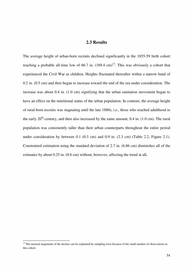
54

2.3 Results

The average height of urban-born recruits declined significantly in the 1855-59 birth cohort

reaching a probable all-time low of 66.7 in. (169.4 cm)13. This was obviously a cohort that

experienced the Civil War as children. Heights fluctuated thereafter within a narrow band of

0.2 in. (0.5 cm) and then began to increase toward the end of the era under consideration. The

increase was about 0.4 in. (1.0 cm) signifying that the urban sanitation movement began to

have an effect on the nutritional status of the urban population. In contrast, the average height

of rural-born recruits was stagnating until the late 1880s, i.e., those who reached adulthood in

the early 20th-century, and then also increased by the same amount, 0.4 in. (1.0 cm). The rural

population was consistently taller than their urban counterparts throughout the entire period

under consideration by between 0.1 (0.3 cm) and 0.9 in. (2.3 cm) (Table 2.2, Figure 2.1).

Constrained estimation using the standard deviation of 2.7 in. (6.86 cm) diminishes all of the

estimates by about 0.25 in. (0.6 cm) without, however, affecting the trend at all.

13 The unusual magnitude of the decline can be explained by sampling error because of the small number of observations in

this cohort.

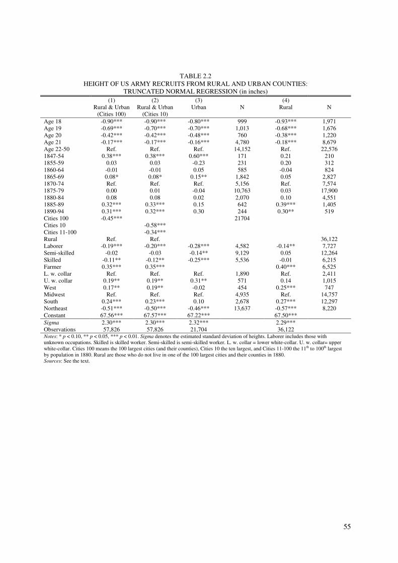
55

TABLE 2.2 HEIGHT OF US ARMY RECRUITS FROM RURAL AND URBAN COUNTIES:

TRUNCATED NORMAL REGRESSION (in inches) (1) (2) (3) (4) Rural & Urban

(Cities 100) Rural & Urban

(Cities 10) Urban N Rural N

Age 18 -0.90*** -0.90*** -0.80*** 999 -0.93*** 1,971 Age 19 -0.69*** -0.70*** -0.70*** 1,013 -0.68*** 1,676 Age 20 -0.42*** -0.42*** -0.48*** 760 -0.38*** 1,220 Age 21 -0.17*** -0.17*** -0.16*** 4,780 -0.18*** 8,679 Age 22-50 Ref. Ref. Ref. 14,152 Ref. 22,576 1847-54 0.38*** 0.38*** 0.60*** 171 0.21 210 1855-59 0.03 0.03 -0.23 231 0.20 312 1860-64 -0.01 -0.01 0.05 585 -0.04 824 1865-69 0.08* 0.08* 0.15** 1,842 0.05 2,827 1870-74 Ref. Ref. Ref. 5,156 Ref. 7,574 1875-79 0.00 0.01 -0.04 10,763 0.03 17,900 1880-84 0.08 0.08 0.02 2,070 0.10 4,551 1885-89 0.32*** 0.33*** 0.15 642 0.39*** 1,405 1890-94 0.31*** 0.32*** 0.30 244 0.30** 519 Cities 100 -0.45*** 21704 Cities 10 -0.58*** Cities 11-100 -0.34*** Rural Ref. Ref. 36,122 Laborer -0.19*** -0.20*** -0.28*** 4,582 -0.14** 7,727 Semi-skilled -0.02 -0.03 -0.14** 9,129 0.05 12,264 Skilled -0.11** -0.12** -0.25*** 5,536 -0.01 6,215 Farmer 0.35*** 0.35*** 0.40*** 6,525 L. w. collar Ref. Ref. Ref. 1,890 Ref. 2,411 U. w. collar 0.19** 0.19** 0.31** 571 0.14 1,015 West 0.17** 0.19** -0.02 454 0.25*** 747 Midwest Ref. Ref. Ref. 4,935 Ref. 14,757 South 0.24*** 0.23*** 0.10 2,678 0.27*** 12,297 Northeast -0.51*** -0.50*** -0.46*** 13,637 -0.57*** 8,220 Constant 67.56*** 67.57*** 67.22*** 67.50*** Sigma 2.30*** 2.30*** 2.32*** 2.29*** Observations 57,826 57,826 21,704 36,122 Notes: * p < 0.10, ** p < 0.05, *** p < 0.01. Sigma denotes the estimated standard deviation of heights. Laborer includes those with unknown occupations. Skilled is skilled worker. Semi-skilled is semi-skilled worker. L. w. collar = lower white-collar. U. w. collar= upper white-collar. Cities 100 means the 100 largest cities (and their counties), Cities 10 the ten largest, and Cities 11-100 the 11th to 100th largest by population in 1880. Rural are those who do not live in one of the 100 largest cities and their counties in 1880. Sources: See the text.

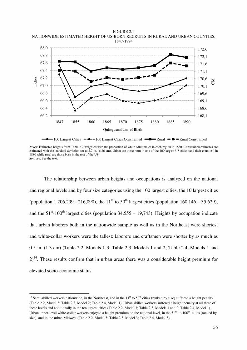
56

FIGURE 2.1 NATIONWIDE ESTIMATED HEIGHT OF US-BORN RECRUITS IN RURAL AND URBAN COUNTIES,

1847-1894

Notes: Estimated heights from Table 2.2 weighted with the proportion of white adult males in each region in 1880. Constrained estimates are estimated with the standard deviation set to 2.7 in. (6.86 cm). Urban are those born in one of the 100 largest US cities (and their counties) in 1880 while rural are those born in the rest of the US. Sources: See the text.

The relationship between urban heights and occupations is analyzed on the national

and regional levels and by four size categories using the 100 largest cities, the 10 largest cities

(population 1,206,299 - 216,090), the 11th to 50th largest cities (population 160,146 – 35,629),

and the 51st-100th largest cities (population 34,555 – 19,743). Heights by occupation indicate

that urban laborers both in the nationwide sample as well as in the Northeast were shortest

and white-collar workers were the tallest: laborers and craftsmen were shorter by as much as

0.5 in. (1.3 cm) (Table 2.2, Models 1-3; Table 2.3, Models 1 and 2; Table 2.4, Models 1 and

2)14. These results confirm that in urban areas there was a considerable height premium for

elevated socio-economic status.

14 Semi-skilled workers nationwide, in the Northeast, and in the 11th to 50th cities (ranked by size) suffered a height penalty

(Table 2.2, Model 3; Table 2.3, Model 2; Table 2.4, Model 1). Urban skilled workers suffered a height penalty at all three of

these levels and additionally in the ten largest cities (Table 2.2, Model 3; Table 2.3, Models 1 and 2; Table 2.4, Model 1).

Urban upper-level white-collar workers enjoyed a height premium on the national level, in the 51st to 100th cities (ranked by

size), and in the urban Midwest (Table 2.2, Model 3; Table 2.3, Model 3; Table 2.4, Model 3).

168,1

168,6

169,1

169,6

170,1

170,6

171,1

171,6

172,1

172,6

66,2

66,4

66,6

66,8

67,0

67,2

67,4

67,6

67,8

68,0

1847 1855 1860 1865 1870 1875 1880 1885 1890

CM

Inch

es

Quinquennium of Birth

100 Largest Cities 100 Largest Cities Constrained Rural Rural Constrained

57

TABLE 2.3 HEIGHT OF US ARMY RECRUITS BY DIFFERENT CITY SIZES:

TRUNCATED NORMAL REGRESSION (in inches) (1) (2) (3) Cities

1-10 N Cities

11-50 N Cities

51-100 N

Age 18 -0.64*** 423 -0.79*** 318 -0.82*** 278 Age 19 -0.65*** 423 -0.69*** 347 -0.70*** 263 Age 20 -0.37** 314 -0.45*** 261 -0.67*** 193 Age 21 -0.13* 2,216 -0.15 1,606 -0.17 1,037 Age 22-50 Ref. 6,534 Ref. 4,753 Ref. 3,382 1847-59 0.23 189 -0.11 136 0.90*** 100 1860-64 -0.36* 275 0.48** 194 0.18 151 1865-69 0.04 828 0.27** 604 0.21 471 1870-74 Ref. 2,324 Ref. 1,772 Ref. 1,255 1875-79 -0.01 5,032 0.00 3,577 -0.13 2,437 1880-84 -0.07 837 0.04 701 0.02 577 1885-94 0.28* 425 0.18 301 -0.14 162 Laborer -0.31*** 1,888 -0.53*** 1,623 0.06 1,172 Semi-skilled -0.10 4,246 -0.33** 3,063 -0.01 2,085 Skilled -0.25** 2,504 -0.47*** 1,874 0.00 1,345 L. w. collar Ref. 991 Ref. 548 Ref. 416 U. w. collar 0.24 282 0.19 179 0.47* 136 West -0.03 321 -0.64 53 0.47* 80 Midwest Ref. 2,349 Ref. 1,324 Ref. 766 South -0.17 740 0.12 1,289 0.02 649 Northeast -0.54*** 6,500 -0.39*** 4,619 -0.70*** 3,658 Constant 67.14*** 67.47*** 67.28*** Sigma 2.30*** 2.30*** 2.34*** Observations 9,910 7,285 5,153

Notes: * p < 0.10, ** p < 0.05, *** p < 0.01. Sigma denotes the estimated standard deviation of heights. Laborer includes those with unknown occupations. Skilled is skilled worker. Semi-skilled is semi-skilled worker. L. w. collar is lower white-collar. U. w. collar is upper white-collar. Cities 1-10 means the ten largest cities by population (and their counties), Cities 11-50 the 11th to 50th, and Cities 51-100 the 51st to 100th largest in 1880. Sources: See the text.

FIGURE 2.2 NATIONWIDE ESTIMATED HEIGHT OF US-BORN RECRUITS IN THE 100 LARGEST URBAN

COUNTIES, 1847-1894

Notes: Estimated heights from Table 2.3 weighted with the proportion of white adult males in each region in 1880. 1 to 10 are the 10 largest, 11 to 50 are the 11th- 50th largest, and 51 to 100 are the 51st- 100th largest cities by population and their counties in 1880. Sources: See the text.

167,6

168,6

169,6

170,6

171,6

172,6

173,6

66,0

66,5

67,0

67,5

68,0

68,5

1847-59 1860-64 1865-69 1870-74 1875-79 1880-84 1885-94

CM

Inch

es

Birth Cohort

1 to 10 11 to 50 51 to 100

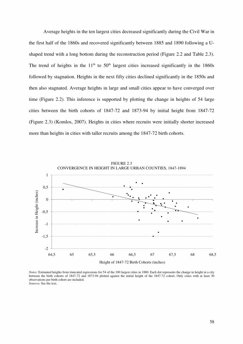
58

Average heights in the ten largest cities decreased significantly during the Civil War in

the first half of the 1860s and recovered significantly between 1885 and 1890 following a U-

shaped trend with a long bottom during the reconstruction period (Figure 2.2 and Table 2.3).

The trend of heights in the 11th to 50th largest cities increased significantly in the 1860s

followed by stagnation. Heights in the next fifty cities declined significantly in the 1850s and

then also stagnated. Average heights in large and small cities appear to have converged over

time (Figure 2.2). This inference is supported by plotting the change in heights of 54 large

cities between the birth cohorts of 1847-72 and 1873-94 by initial height from 1847-72

(Figure 2.3) (Komlos, 2007). Heights in cities where recruits were initially shorter increased

more than heights in cities with taller recruits among the 1847-72 birth cohorts.

FIGURE 2.3 CONVERGENCE IN HEIGHT IN LARGE URBAN COUNTIES, 1847-1894

Notes: Estimated heights from truncated regressions for 54 of the 100 largest cities in 1880. Each dot represents the change in height in a city between the birth cohorts of 1847-72 and 1873-94 plotted against the initial height of the 1847-72 cohort. Only cities with at least 30 observations per birth cohort are included. Sources: See the text.

-2

-1,5

-1

-0,5

0

0,5

1

64,5 65 65,5 66 66,5 67 67,5 68 68,5

Incr

ease

in H

eigh

t (in

ches

)

Height of 1847-72 Birth Cohorts (inches)

59

TABLE 2.4 HEIGHT OF US ARMY RECRUITS BY CENSUS REGION:

TRUNCATED NORMAL REGRESSION (in inches)

(1) (2) (3) (4) (5) (6) Northeast Urban N Northeast Rural N Midwest Urban N Midwest Rural N South Urban N South Rural N Age 18 -0.91*** 600 -0.78*** 474 -0.56*** 280 -0.98*** 870 -1.10*** 93 -1.15*** 580 Age 19 -0.63*** 626 -0.91*** 391 -0.72*** 221 -0.59*** 700 -1.14*** 140 -0.78*** 550 Age 20 -0.46*** 439 -0.27 254 -0.73*** 216 -0.27** 508 -0.26 92 -0.61*** 424 Age 21 -0.22*** 3,052 -0.14 1,843 -0.07 1,152 -0.17*** 3,660 -0.24* 492 -0.21*** 2,956 Age 22-50 Ref. 8,920 Ref. 5,258 3,066 Ref. 9,019 Ref. 1,861 Ref. 7,787 1847-54 0.89*** 112 0.82*** 75 1855-59 0.00 156 0.27 91 1860-64 -0.19 373 -0.16 227 1865-69 0.16 1,121 0.05 751 1870-74 Ref. 3,300 Ref. 1,768 1875-79 -0.02 6,777 -0.08 4,017 1880-84 0.02 1,298 -0.06 921 1885-89 0.10 352 0.24 261 1890-94 0.36 148 0.04 109 1847-64 -0.37 178 0.12 463 0.66*** 156 -0.19 471 1865-79 Ref. 3,963 Ref. 11,672 Ref. 2,211 Ref. 9,424 1880-94 -0.01 794 0.18*** 2,622 0.29 311 0.19*** 2,402 Laborer -0.40*** 2,874 -0.44*** 1,943 -0.10 1,062 -0.10 3,078 -0.19 593 -0.09 2,527 Semi-skilled -0.24*** 5,803 -0.24** 3,110 -0.04 1,985 0.09 4,576 -0.02 1,170 0.17 4,265 Skilled -0.38*** 3,520 -0.21 1,799 -0.14 1,286 -0.11 2,626 -0.05 616 0.18 1,614 L. w. collar Ref. 1,090 Ref. 559 Ref. 471 Ref. 1,062 Ref. 235 Ref. 686 U. w. collar 0.18 353 -0.03 182 0.43* 132 -0.05 423 0.29 64 0.37** 381 Farmer 0.22 645 0.27*** 2,996 0.62*** 2,836 City pop. -0.03*** -0.04* -0.22*** Constant 67.00*** 67.19*** 67.22*** 67.55*** 67.45*** 67.69*** Sigma 2.32*** 2.34*** 2.30*** 2.27*** 2.37*** 2.28*** Observations 13,637 8,220 4,935 14,757 2,678 12,297 Notes: * p < 0.10, ** p < 0.05, *** p < 0.01. Sigma denotes the estimated standard deviation of heights. Laborer includes those with unknown occupations. Skilled is skilled worker. Semi-skilled is semi-skilled worker. L. w. collar is lower white-collar. U. w. collar is upper white-collar. Urban are those living in one of the 100 largest cities (and their counties). Rural are all those living outside of the 100 largest cities (and their counties) in 1880. City pop. is the population living in cities (in 100,000 people). Sources: See the text.

60

FIGURE 2.4 ESTIMATED HEIGHT OF URBAN RECRUITS BY CENSUS REGIONS, 1847-1894

Notes: Estimated heights from Table 2.4. Quinquennia of birth used in Northeast and decades of birth used in Midwest and South. Sources: Table 2.4.

Spatial analysis indicates that while average height of urban recruits from the

Northeast declined significantly in the late 1850s and then stagnated conforming to the

national pattern, that of Midwesterners only stagnated, whereas that of Southern recruits, who

were tallest, dipped between 1865 and 1879 (Table 2.4 and Figure 2.4).

We also estimate height trends separately in those cities (within the 100 largest cities)

with more than 30 observations per birth cohort per city in the sample (Figure 2.5). Heights in

all these cities did not change significantly over time with the exception of a decrease in

Boston. Height differences among cities were considerable. In the 1865-79 cohort recruits

from St. Louis were 0.67 in. (1.7 cm) taller than recruits from Philadelphia and 0.59 in. (1.5

cm) taller than those from New York (Tables 2.5, 2.6, and Figure 2.5). Average heights in the

largest cities were shortest while heights in Midwestern cities were tallest. For instance, the

tallest recruits were natives of St. Louis, MO, and Cincinnati, OH, the 6th and 8th cities,

respectively, in terms of size, while the shortest (born between 1865 and 1879) were from the

two largest cities, New York and Philadelphia (Figure 2.5).

168,1

168,6

169,1

169,6

170,1

170,6

171,1

171,6

172,1

66,2

66,4

66,6

66,8

67,0

67,2

67,4

67,6

67,8

1847 1855 1860 1865 1870 1875 1880 1885 1890

CM

Inch

es

Quinquennium of Birth

Northeast Midwest South

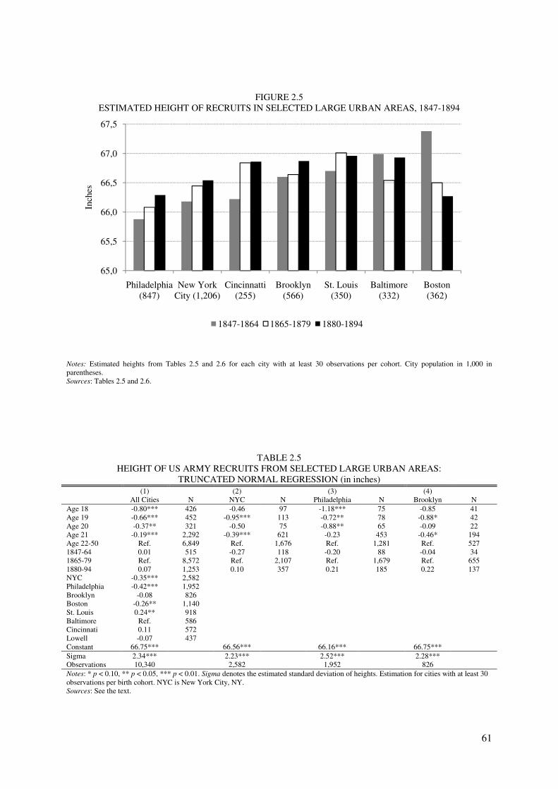
61

FIGURE 2.5 ESTIMATED HEIGHT OF RECRUITS IN SELECTED LARGE URBAN AREAS, 1847-1894

Notes: Estimated heights from Tables 2.5 and 2.6 for each city with at least 30 observations per cohort. City population in 1,000 in parentheses. Sources: Tables 2.5 and 2.6.

TABLE 2.5 HEIGHT OF US ARMY RECRUITS FROM SELECTED LARGE URBAN AREAS:

TRUNCATED NORMAL REGRESSION (in inches) (1) (2) (3) (4) All Cities N NYC N Philadelphia N Brooklyn N Age 18 -0.80*** 426 -0.46 97 -1.18*** 75 -0.85 41 Age 19 -0.66*** 452 -0.95*** 113 -0.72** 78 -0.88* 42 Age 20 -0.37** 321 -0.50 75 -0.88** 65 -0.09 22 Age 21 -0.19*** 2,292 -0.39*** 621 -0.23 453 -0.46* 194 Age 22-50 Ref. 6,849 Ref. 1,676 Ref. 1,281 Ref. 527 1847-64 0.01 515 -0.27 118 -0.20 88 -0.04 34 1865-79 Ref. 8,572 Ref. 2,107 Ref. 1,679 Ref. 655 1880-94 0.07 1,253 0.10 357 0.21 185 0.22 137 NYC -0.35*** 2,582 Philadelphia -0.42*** 1,952 Brooklyn -0.08 826 Boston -0.26** 1,140 St. Louis 0.24** 918 Baltimore Ref. 586 Cincinnati 0.11 572 Lowell -0.07 437 Constant 66.75*** 66.56*** 66.16*** 66.75*** Sigma 2.34*** 2.23*** 2.52*** 2.28*** Observations 10,340 2,582 1,952 826 Notes: * p < 0.10, ** p < 0.05, *** p < 0.01. Sigma denotes the estimated standard deviation of heights. Estimation for cities with at least 30 observations per birth cohort. NYC is New York City, NY. Sources: See the text.

65,0

65,5

66,0

66,5

67,0

67,5

Philadelphia (847)

New York City (1,206)

Cincinnatti (255)

Brooklyn (566)

St. Louis (350)

Baltimore (332)

Boston (362)

Inch

es

1847-1864 1865-1879 1880-1894

62

TABLE 2.6 HEIGHT OF US ARMY RECRUITS FROM SELECTED LARGE URBAN AREAS:

TRUNCATED NORMAL REGRESSION (in inches)

(1) (2) (3) (4) Boston N St. Louis N Baltimore N Cincinnati N Age 18 -0.39 55 -0.66 56 -2.26*** 25 -0.89 28 Age 19 -0.27 48 -0.83* 40 -0.43 26 -0.49 30 Age 20 -0.28 30 -0.26 46 0.92* 16 -0.24 17 Age 21 0.23 212 -0.04 219 -0.21 105 0.48* 121 Age 22-50 Ref. 795 Ref. 557 Ref. 414 Ref. 376 1847-64 0.88*** 68 -0.30 36 0.45 30 -0.62 48 1865-79 Ref. 948 Ref. 763 Ref. 491 Ref. 459 1880-94 -0.24 124 -0.05 119 0.40 65 0.03 65 Constant 66.47*** 67.03*** 66.55*** 66.74*** Sigma 2.21*** 2.27*** 2.37*** 2.36*** Observations 1,140 918 586 572 Notes: * p < 0.10, ** p < 0.05, *** p < 0.01. Sigma denotes the estimated standard deviation of heights. Estimation for cities with at least 30 observations per birth cohort. Sources: See the text.

Scatter plots of city size against height exhibit no clear relationship. However, if one

excludes the four largest cities (with more than 400,000 inhabitants), there emerges a negative

relationship for the 1847-64 and the 1880-94 birth cohorts (Figure 2.6). Estimates from a

polynomial regression with height regressed on population in linear, quadratic, and cubic

form paint a clearer picture of the relationship (Table 2.7). In the middle of the 19th-century

the best place to live in terms of height were small cities, while in the end of the 19th-century

it was in larger cities with about 250,000 inhabitants, but not in the largest cities. In the 1847-

64 birth cohort the relationship can be described by a downward sloping curve that is

flattening out implying that heights decreased with increases in city population, but at a

decreasing rate. This relationship is fundamentally different in the 1880-94 birth cohort where

there was an inverse U-shaped relationship between height and city size with a maximum

height in cities with about 250,000 inhabitants and declining heights thereafter (Figure 2.6).

This suggests that this relationship was non-linear and that circumstances in larger cities

relative to small cities had improved by the end of the 19th-century. However, recruits from

the largest cities remained the shortest.

63

FIGURE 2.6 SCATTERPLOTS OF HEIGHT AND ESTIMATED HEIGHT BY CITY SIZE

Scatter plot of height by city size for 100 largest urban counties, 1847-64

Scatter plot of height by city size for urban counties with cities of up to 400,000 inhabitants, 1847-64

Scatter plot of height by city size for 100 largest urban

counties, 1880-94 Scatter plot of height by city size for urban counties with

cities of up to 400,000 inhabitants, 1880-94

Estimated heights by city size (1847-64),

with quadratic population from polynomial regression Estimated heights by city size (1847-64),

with quadratic and cubic population from polynomial regression

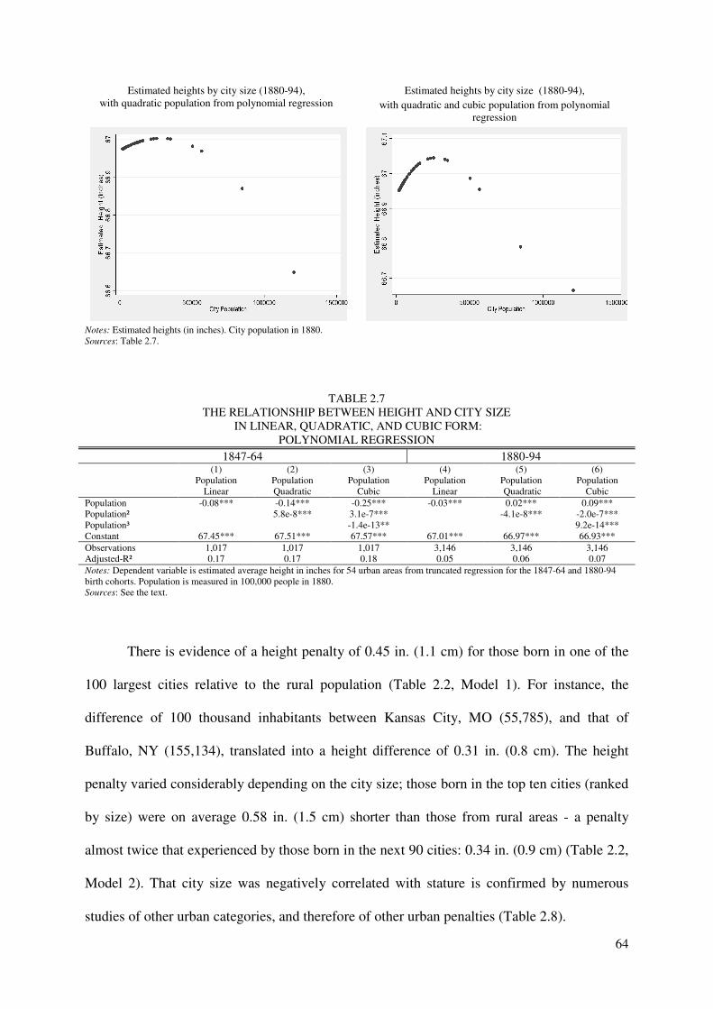
64

Estimated heights by city size (1880-94), with quadratic population from polynomial regression

Estimated heights by city size (1880-94),

with quadratic and cubic population from polynomial regression

Notes: Estimated heights (in inches). City population in 1880. Sources: Table 2.7.

TABLE 2.7 THE RELATIONSHIP BETWEEN HEIGHT AND CITY SIZE

IN LINEAR, QUADRATIC, AND CUBIC FORM: POLYNOMIAL REGRESSION

1847-64 1880-94 (1) (2) (3) (4) (5) (6) Population

Linear Population Quadratic

Population Cubic

Population Linear

Population Quadratic

Population Cubic

Population -0.08*** -0.14*** -0.25*** -0.03*** 0.02*** 0.09*** Population² 5.8e-8*** 3.1e-7*** -4.1e-8*** -2.0e-7*** Population³ -1.4e-13** 9.2e-14*** Constant 67.45*** 67.51*** 67.57*** 67.01*** 66.97*** 66.93*** Observations 1,017 1,017 1,017 3,146 3,146 3,146 Adjusted-R² 0.17 0.17 0.18 0.05 0.06 0.07 Notes: Dependent variable is estimated average height in inches for 54 urban areas from truncated regression for the 1847-64 and 1880-94 birth cohorts. Population is measured in 100,000 people in 1880. Sources: See the text.

There is evidence of a height penalty of 0.45 in. (1.1 cm) for those born in one of the

100 largest cities relative to the rural population (Table 2.2, Model 1). For instance, the

difference of 100 thousand inhabitants between Kansas City, MO (55,785), and that of

Buffalo, NY (155,134), translated into a height difference of 0.31 in. (0.8 cm). The height

penalty varied considerably depending on the city size; those born in the top ten cities (ranked

by size) were on average 0.58 in. (1.5 cm) shorter than those from rural areas - a penalty

almost twice that experienced by those born in the next 90 cities: 0.34 in. (0.9 cm) (Table 2.2,

Model 2). That city size was negatively correlated with stature is confirmed by numerous

studies of other urban categories, and therefore of other urban penalties (Table 2.8).

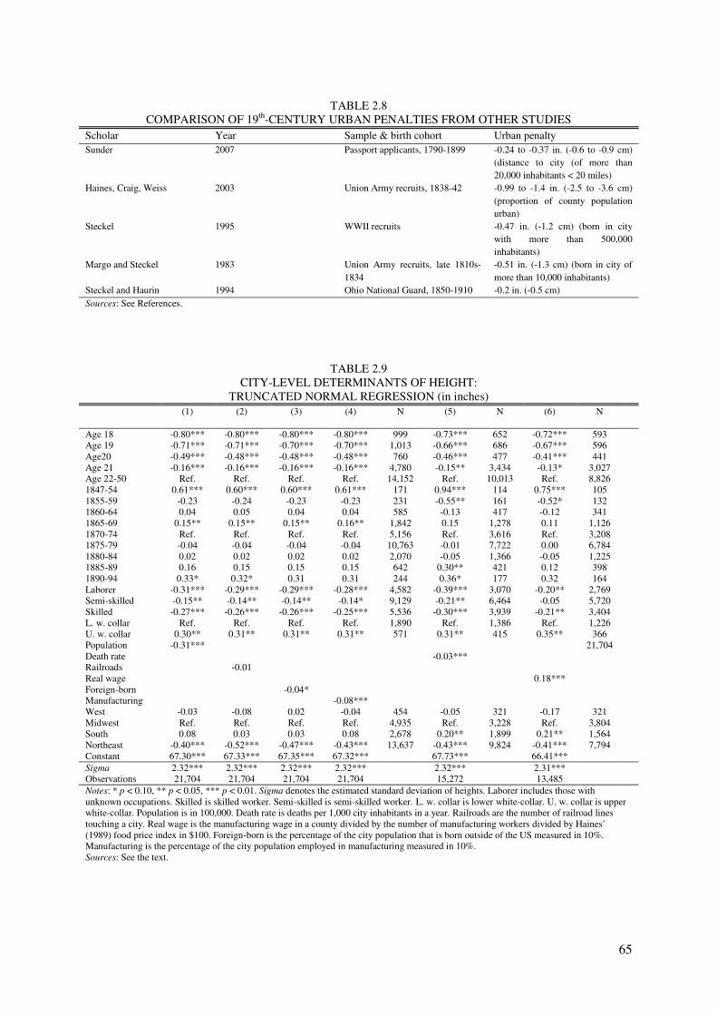
65

TABLE 2.8

COMPARISON OF 19th-CENTURY URBAN PENALTIES FROM OTHER STUDIES

Scholar Year Sample & birth cohort Urban penalty Sunder 2007 Passport applicants, 1790-1899 -0.24 to -0.37 in. (-0.6 to -0.9 cm)

(distance to city (of more than 20,000 inhabitants < 20 miles)

Haines, Craig, Weiss 2003 Union Army recruits, 1838-42 -0.99 to -1.4 in. (-2.5 to -3.6 cm)

(proportion of county population urban)

Steckel 1995 WWII recruits -0.47 in. (-1.2 cm) (born in city with more than 500,000 inhabitants)

Margo and Steckel 1983 Union Army recruits, late 1810s-

1834

-0.51 in. (-1.3 cm) (born in city of

more than 10,000 inhabitants) Steckel and Haurin 1994 Ohio National Guard, 1850-1910 -0.2 in. (-0.5 cm)

Sources: See References.

TABLE 2.9 CITY-LEVEL DETERMINANTS OF HEIGHT:

TRUNCATED NORMAL REGRESSION (in inches)

(1) (2) (3) (4) N (5) N (6) N Age 18 -0.80*** -0.80*** -0.80*** -0.80*** 999 -0.73*** 652 -0.72*** 593 Age 19 -0.71*** -0.71*** -0.70*** -0.70*** 1,013 -0.66*** 686 -0.67*** 596 Age20 -0.49*** -0.48*** -0.48*** -0.48*** 760 -0.46*** 477 -0.41*** 441 Age 21 -0.16*** -0.16*** -0.16*** -0.16*** 4,780 -0.15** 3,434 -0.13* 3,027 Age 22-50 Ref. Ref. Ref. Ref. 14,152 Ref. 10,013 Ref. 8,826 1847-54 0.61*** 0.60*** 0.60*** 0.61*** 171 0.94*** 114 0.75*** 105 1855-59 -0.23 -0.24 -0.23 -0.23 231 -0.55** 161 -0.52* 132 1860-64 0.04 0.05 0.04 0.04 585 -0.13 417 -0.12 341 1865-69 0.15** 0.15** 0.15** 0.16** 1,842 0.15 1,278 0.11 1,126 1870-74 Ref. Ref. Ref. Ref. 5,156 Ref. 3,616 Ref. 3,208 1875-79 -0.04 -0.04 -0.04 -0.04 10,763 -0.01 7,722 0.00 6,784 1880-84 0.02 0.02 0.02 0.02 2,070 -0.05 1,366 -0.05 1,225 1885-89 0.16 0.15 0.15 0.15 642 0.30** 421 0.12 398 1890-94 0.33* 0.32* 0.31 0.31 244 0.36* 177 0.32 164 Laborer -0.31*** -0.29*** -0.29*** -0.28*** 4,582 -0.39*** 3,070 -0.20** 2,769 Semi-skilled -0.15** -0.14** -0.14** -0.14* 9,129 -0.21** 6,464 -0.05 5,720 Skilled -0.27*** -0.26*** -0.26*** -0.25*** 5,536 -0.30*** 3,939 -0.21** 3,404 L. w. collar Ref. Ref. Ref. Ref. 1,890 Ref. 1,386 Ref. 1,226 U. w. collar 0.30** 0.31** 0.31** 0.31** 571 0.31** 415 0.35** 366 Population -0.31*** 21,704 Death rate -0.03*** Railroads -0.01 Real wage 0.18*** Foreign-born -0.04* Manufacturing -0.08*** West -0.03 -0.08 0.02 -0.04 454 -0.05 321 -0.17 321 Midwest Ref. Ref. Ref. Ref. 4,935 Ref. 3,228 Ref. 3,804 South 0.08 0.03 0.03 0.08 2,678 0.20** 1,899 0.21** 1,564 Northeast -0.40*** -0.52*** -0.47*** -0.43*** 13,637 -0.43*** 9,824 -0.41*** 7,794 Constant 67.30*** 67.33*** 67.35*** 67.32*** 67.73*** 66.41*** Sigma 2.32*** 2.32*** 2.32*** 2.32*** 2.32*** 2.31*** Observations 21,704 21,704 21,704 21,704 15,272 13,485 Notes: * p < 0.10, ** p < 0.05, *** p < 0.01. Sigma denotes the estimated standard deviation of heights. Laborer includes those with unknown occupations. Skilled is skilled worker. Semi-skilled is semi-skilled worker. L. w. collar is lower white-collar. U. w. collar is upper white-collar. Population is in 100,000. Death rate is deaths per 1,000 city inhabitants in a year. Railroads are the number of railroad lines touching a city. Real wage is the manufacturing wage in a county divided by the number of manufacturing workers divided by Haines’ (1989) food price index in $100. Foreign-born is the percentage of the city population that is born outside of the US measured in 10%. Manufacturing is the percentage of the city population employed in manufacturing measured in 10%. Sources: See the text.

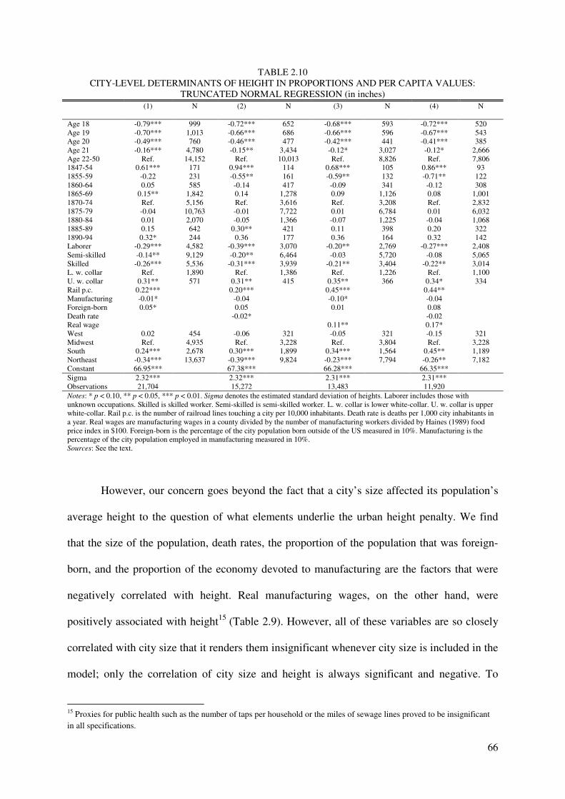
66

TABLE 2.10 CITY-LEVEL DETERMINANTS OF HEIGHT IN PROPORTIONS AND PER CAPITA VALUES:

TRUNCATED NORMAL REGRESSION (in inches)

(1) N (2) N (3) N (4) N Age 18 -0.79*** 999 -0.72*** 652 -0.68*** 593 -0.72*** 520 Age 19 -0.70*** 1,013 -0.66*** 686 -0.66*** 596 -0.67*** 543 Age 20 -0.49*** 760 -0.46*** 477 -0.42*** 441 -0.41*** 385 Age 21 -0.16*** 4,780 -0.15** 3,434 -0.12* 3,027 -0.12* 2,666 Age 22-50 Ref. 14,152 Ref. 10,013 Ref. 8,826 Ref. 7,806 1847-54 0.61*** 171 0.94*** 114 0.68*** 105 0.86*** 93 1855-59 -0.22 231 -0.55** 161 -0.59** 132 -0.71** 122 1860-64 0.05 585 -0.14 417 -0.09 341 -0.12 308 1865-69 0.15** 1,842 0.14 1,278 0.09 1,126 0.08 1,001 1870-74 Ref. 5,156 Ref. 3,616 Ref. 3,208 Ref. 2,832 1875-79 -0.04 10,763 -0.01 7,722 0.01 6,784 0.01 6,032 1880-84 0.01 2,070 -0.05 1,366 -0.07 1,225 -0.04 1,068 1885-89 0.15 642 0.30** 421 0.11 398 0.20 322 1890-94 0.32* 244 0.36 177 0.36 164 0.32 142 Laborer -0.29*** 4,582 -0.39*** 3,070 -0.20** 2,769 -0.27*** 2,408 Semi-skilled -0.14** 9,129 -0.20** 6,464 -0.03 5,720 -0.08 5,065 Skilled -0.26*** 5,536 -0.31*** 3,939 -0.21** 3,404 -0.22** 3,014 L. w. collar Ref. 1,890 Ref. 1,386 Ref. 1,226 Ref. 1,100 U. w. collar 0.31** 571 0.31** 415 0.35** 366 0.34* 334 Rail p.c. 0.22*** 0.20*** 0.45*** 0.44** Manufacturing -0.01* -0.04 -0.10* -0.04 Foreign-born 0.05* 0.05 0.01 0.08 Death rate -0.02* -0.02 Real wage 0.11** 0.17* West 0.02 454 -0.06 321 -0.05 321 -0.15 321 Midwest Ref. 4,935 Ref. 3,228 Ref. 3,804 Ref. 3,228 South 0.24*** 2,678 0.30*** 1,899 0.34*** 1,564 0.45** 1,189 Northeast -0.34*** 13,637 -0.39*** 9,824 -0.23*** 7,794 -0.26** 7,182 Constant 66.95*** 67.38*** 66.28*** 66.35*** Sigma 2.32*** 2.32*** 2.31*** 2.31*** Observations 21,704 15,272 13,483 11,920 Notes: * p < 0.10, ** p < 0.05, *** p < 0.01. Sigma denotes the estimated standard deviation of heights. Laborer includes those with unknown occupations. Skilled is skilled worker. Semi-skilled is semi-skilled worker. L. w. collar is lower white-collar. U. w. collar is upper white-collar. Rail p.c. is the number of railroad lines touching a city per 10,000 inhabitants. Death rate is deaths per 1,000 city inhabitants in a year. Real wages are manufacturing wages in a county divided by the number of manufacturing workers divided by Haines (1989) food price index in $100. Foreign-born is the percentage of the city population born outside of the US measured in 10%. Manufacturing is the percentage of the city population employed in manufacturing measured in 10%. Sources: See the text.

However, our concern goes beyond the fact that a city’s size affected its population’s

average height to the question of what elements underlie the urban height penalty. We find

that the size of the population, death rates, the proportion of the population that was foreign-

born, and the proportion of the economy devoted to manufacturing are the factors that were

negatively correlated with height. Real manufacturing wages, on the other hand, were

positively associated with height15 (Table 2.9). However, all of these variables are so closely

correlated with city size that it renders them insignificant whenever city size is included in the

model; only the correlation of city size and height is always significant and negative. To

15 Proxies for public health such as the number of taps per household or the miles of sewage lines proved to be insignificant

in all specifications.

67

compensate for this effect while also countering multicollinearity, we use proportions and per

capita values of variables (Table 2.10).

We find robust positive associations for the real (manufacturing) wage per capita in all

specifications. A $100-per-annum (27% of average income) increase in real wages translated

into better housing and nutrition, which in turn translated into a height increase of between

0.11 and 0.17 in. (0.3-0.4 cm), between 24% and 38% of the urban penalty16. A decrease in

the death rate by 10 deaths per 1,000 people (45% of average death rate) was correlated with a

height increase of 0.20 in. (0.5 cm) or 49% of the urban penalty: i.e., the worse the disease

environment, the lower the population’s average height17. The percentage of foreign-born

residents changes the sign (compared with Table 2.9) and is significant and positive only in

Model 1 (Table 2.10). The percentage in manufacturing is significant only in Models 1 and 3,

but always negative: a ten percentage point (63% of average) increase in employment in the

manufacturing sector yielded a height decrease of 0.01-0.10 in. (0.03-0.3 cm) or between 2

and 22 percent of the urban penalty, confirming that there was a negative association between

manufacturing work and height.

The number of railroad connections of a city per 10,000 inhabitants was positively

correlated with height; every additional railroad line per 10,000 inhabitants (250% of average)

meant a height increase of 0.20 to 0.45 in. (0.5-1.1 cm), between 44 and 100 percent of the

urban penalty. The railroad-height correlation therefore supports the theory that railroads, by

facilitating the importing of foodstuffs from agricultural regions, led to an improvement in

city dwellers’ nutrition, because this positive correlation still holds when controlling for death

16 The urban penalty from Table 2.2, Model 1 for living in one of the 100 largest urban counties is used. Averages from Table

2.1 are used

17 The death rate ceases being significant when real wage is included. This could be because including the variable real wage

greatly reduces the sample size.

68

rates, real wages, the share of foreign-born, and the percentage in manufacturing that proxy

diseases and living conditions.

Evidently, of all the elements considered, it was the size of a city that always had a

negative impact on height. However, this effect was indirect, channeled through net nutrition

and diseases. On the individual level, superior social status measured by occupations

constituted a height advantage roughly equivalent to an additional railroad line or a 100,000-

person decrease in the size of the city’s population.

2.4 Conclusion

This study finds that recruits born in rural regions were consistently taller than those born in

cities. Urban heights declined significantly after 1855 and then stagnated, in the main,

whereas rural heights were stagnating until the late 1880s, at which point they began to

increase significantly. In the second half of the 19th-century there was an urban height penalty

of between 0.58 in. (1.5 cm) in the ten largest cities and 0.34 in. (0.9 cm) in the next ninety

cities (ranked by size). This penalty is of a similar magnitude as in other studies. We find

evidence that average urban heights converged over time with heights in larger cities

approaching those in smaller ones: While in the 1850s and 1860s heights decreased with city

size at a decreasing rate, in the late 19th-century we find this relationship to be inversely U-

shaped with largest heights in cities of about 250,000 inhabitants. Above-average socio-

economic status, in the form of upper-level white-collar occupations, was correlated with

above-average height in cities.

However, it was not a city’s size itself that mattered but the quality of the environment

that correlated with city size. A large number of factors contributed including sanitation,

canalization, and running water, rather than the fact that railroad access and height were

69

positively correlated. This is because expansion of the transportation network meant increased

market integration, which decreased the price and increased the quality of the food that city

dwellers purchased and consumed, and this improvement in their nutrition led to their

enjoying a height advantage18. Since real wages determined the affordability of food and

housing, their level was positively correlated with height, as opposed to death rates, which

were negatively correlated with height. Industrialization, too, as measured by the share of the

urban population working in the manufacturing sector, was negatively correlated with stature

because the working conditions and disease environment in factories compared unfavorably

with those of small-scale, rural manufacturing.

An interesting question is how much each of these factors contributed to the height

difference between large and small cities and between urban and rural regions: the difference

in real wages between the ten largest cities and the next 90 amounts to 8 percent of the height

difference between these two groups of cities. The difference between the average number of

railroads per capita in the ten largest cities (0.24) and in the next 90 (0.99) amounts to 0.15 in.

(0.4 cm), or about 58% of the height penalty between these two groups of cities19. The

difference between the crude death rate in urban areas (24.7) and rural areas (18.8) accounts

for a height difference of 0.18 in. (0.5 cm), or about 40 percent of the urban penalty20 (Haines,

2001). The difference between the share of the work force in manufacturing nationwide (6%)

and in cities (16%) accounts for 18 percent of the urban penalty (U.S. Bureau of the Census,

1975; Lebergott, 1984).

Unlike data from the French and Indian War (1754-63), data from the Revolutionary

War (1775-83) reveal an urban height penalty, of 0.9 in. (2.3 cm), which continued not only

18 A similar pattern for water transportation in urban areas has been identified by Yoo (2009).

19 Using sample averages and coefficients from Table 2.10 in relation to the height penalty from Table 2.2.

20 Using 1890 values from registration states that reported death rates (Haines, 2001) with coefficients from Table 2.9 in

relation to the height penalty from Table 2.2.

70

through the Civil War but on into the late 19th-century (Fogel et. al., 1982; Sokoloff and

Villaflor, 1992). In fact, population density continues to be negatively correlated with height

(Komlos and Lauderdale, 2007). Researchers have confirmed that there is an urban penalty in

developed economies such as the UK, too, even when they have controlled for socio-

economic characteristics (Foster, Chinn, and Rona, 1983; Reading, Raybould, and Jarvis,

1993). The significance of this urban height penalty is that it is correlated with elevated

morbidity and mortality risks (Waaler, 1984; Fogel, 1994).

It has been established that the mortality rates of urban and rural populations in the US

during the late-19th and early-20th centuries converged (Condran and Crimmins-Gardner,

1978, 1980, 1983). We find some evidence of a parallel convergence in terms of heights;

however, the difference between urban and rural heights did not decrease in the second half of

the 19th-century but we find that heights in large cities relative to small cities did increase as

sanitary improvements began to affect urban living conditions. A growing railroad network

that was detrimental for rural heights benefitted heights of urban dwellers because food from

rural areas was easily accessible at lower relative prices. In spite of the beginning of a secular

trend that was to last till the middle of the next century, the biological standard of living of

American men, as proxied by their height had still not reached the level they had in the 18th-

century. This is an indication that industrialization even in the New World exerted costs on

the population that were hitherto hidden from view. It took a long time indeed before heights

again reached their pre-industrial level.

71

References

Data:

Minnesota Population Center. 2004. National Historical Geographic Information System

(NHGIS): Pre-release Version 0.1. Minneapolis, MN: University of Minnesota.

http://www.nhgis.org

National Archives and Records Administration. 7th and Pennsylvania Ave., NW,

Washington, DC 20408-0001. Microfilm ID M233. Record Group 094. Register of

Enlistments in the U.S. Army, 1798-1914. Vol 94 (96%), Vol 96 (100%), Vol 97(10%), Vol

98 (93%), Vol 100 (88%),Vol 102 (100%), Vol 103 (80%), Vol 104 (100%), Vol 105 (100%).

U. S. Bureau of the Census. “1880 Census of Population and Housing, Vol. 11, 12, 18, 19.”

http://www.census.gov/prod/www/abs/decennial/1880.htm (accessed February 15th, 2010).

U. S. Bureau of the Census. 1975. Historical Statistics of the United States, Colonial Times

to 1970. Washington, DC: U.S. Government Printing Office.

Literature:

A’Hearn, Brian. 2004. “A restricted maximum likelihood estimator for truncated height

samples.” Economics and Human Biology, 2: 5-19.

Bodnar, John. 1987. The Transplanted: A History of Immigrants in Urban America.

Bloomington, IN: Indiana University Press.

Carson, Scott Alan. 2008. “Nineteenth Century Black and White US Statures: The Primary

Sources of Vitamin D and Their Relationship with Height.” CESifo Working Paper Series No.

2497.

Condran, Gretchen A., and Eileen Crimmins-Gardner. 1978. “Public health measures and

mortality in U.S. cities in the late nineteenth century.” Human Ecology, 6 (1): 27-54.

Condran, Gretchen A., and Eileen Crimmins-Gardner. 1980. “Mortality differentials

between rural and urban areas of states in the northeastern United States 1890–1900.” Journal

of Historical Geography, 6 (2): 179-202.

Crimmins-Gardner, Eileen M., and Gretchen A. Condran. 1983. “Mortality Variation in

U.S. Cities in 1900: A Two-Level Explanation by Cause of Death and Underlying Factors.”

Social Science History, 7 (1): 31-59.

72

Costa, Dora, and Richard Steckel. 1997. “Long-Term Trends in Health, Welfare, and

Economic Growth in the United States.” In: Health and Welfare during Industrialization, ed.

Richard Steckel and Roderick Floud, 47-90. Cambridge, MA: National Bureau of Economic

Research, Inc.

Fogel, Robert W., Stanley L. Engerman, Roderick Floud, Richard H. Steckel, and James

Trussell. 1982. “Changes in American and British Stature since the Mid-Eighteenth Century:

A Preliminary Report on the Usefulness of Data on Height…” NBER Working Papers 0890,

National Bureau of Economic Research, Inc.

Fogel, Robert. 1994. “Economic Growth, Population Theory, and Physiology: the Bearing of

Long-term Processes on the Making of Economic Policy.” American Economic Review, 84:

369–395.

Foster, J. M., S. Chinn, and R.J. Ronja. 1983. “The relation of height of primary school

children to population density.” International Journal of Epidemiology, 12: 199-204.

Frisancho, Robert A. 1990. Anthropometric Standards for the Assessment of Growth and

Nutritional Status. Ann Arbor: University of Michigan Press.

Goldin, Claudia, and Kenneth Sokoloff. 1982. “Women, Children, and Industrialization in

the Early Republic: Evidence from the Manufacturing Censuses.” The Journal of Economic

History, 42: 741-774.

Haines, Michael. 2001. “The Urban Mortality Transition in the United States, 1800-1940.”

Annales de démographie historique, 101 (1): 33-64.

Haines, Michael. 1989. “A State and Local Consumer Price Index for the United States in

1890.” Historical Methods, 22 (3): 97-105.

Haines, Michael, Lee A. Craig, and Thomas Weiss. 2003. “The Short and the Dead:

Nutrition, Mortality, and the ‘Antebellum Puzzle’ in the United States.” Journal of Economic

History, 63: 382-413.

Holick, Michael, 2004. “Sunlight and Vitamin D for Bone Health and Prevention of

Autoimmune Diseases, Cancers, and Cardiovascular Diseases.” American Journal of Clinical

Nutrition, supplement: 1678S-1688S.

Komlos, John. 1987. “The Height and Weight of West Point Cadets: Dietary Change in

Antebellum America.” The Journal of Economic History, 47: 897-927.

73

Komlos, John. 1992. “Toward an Anthropometric History of African-Americans: The Case

of the Free Blacks in Antebellum Maryland.” In: Strategic Factors in Nineteenth Century

American Economic History: A Volume to Honor Robert W. Fogel, ed. Claudia Goldin and

Hugh Rockoff, 297 - 392. Cambridge, MA: National Bureau of Economic Research, Inc.

Komlos, John. 1998. “Shrinking in a Growing Economy? The Mystery of Physical Stature

during the Industrial Revolution.” The Journal of Economic History, 58: 779-802.

Komlos, John. 2004. “Improvements in Maximum Likelihood Estimators of Truncated

Normal Samples with Prior Knowledge of σ. A Simulation Based Study with Application to

Historical Height Samples.” Discussion paper LMU Munich.

Komlos, John. 2007. “Anthropometric evidence on economic growth, biological well-being

and regional convergence in the Habsburg Monarchy, c. 1850–1910.” Cliometrica, 1 (3): 211-

237.

Komlos, John, and Benjamin Lauderdale. 2007. “Underperformance in Affluence: The

Remarkable Relative Decline in U.S. Heights in the Second Half of the 20th Century.” Social

Science Quarterly, 88 (2): 283-305.

Lebergott, Stanley. 1984. The Americans, an economic record. New York City, NY: W.W.

Norton.

Lee, Chulhee. 1997. “Socioeconomic Background, Disease, and Mortality among Union

Army Recruits: Implications for Economic and Demographic History.” Explorations in

Economic History, 34: 27-55.

Margo, Robert, and Richard Steckel. 1983. “Heights of Native Born Northern Whites

during the Antebellum Period.” Journal of Economic History, 43: 167-184.

Preston, Samuel H., and Michael Haines. 1991. Fatal Years: Child Mortality in the Late

Nineteenth-Century America. Princeton, NJ: Princeton University Press.

Reading, Richard, Simon Raybould, and Stephen Jarvis. 1993. “Deprivation, low birth

weight, and children’s height: a comparison between rural and urban areas.” British Medical

Journal, 307: 1458-1462.

Rosen, George. 1944. “The Medical Aspect of the Controversy over Factory Conditions in

New England, 1840-1850.” Bulletin of the History of Medicine, 15 (5): 483-497.

Sokoloff, Kenneth, and Georgia Villaflor. 1982. “The Early Achievement of Modern

Stature in America.” Social Science History, 6 (4): 453-481.

74

Steckel, Richard, and Donald Haurin. 1994. “Health and Nutrition in the American

Midwest: Evidence from the Height of Ohio National Guardsmen, 1850-1910.” In: Stature,

Living Standards, and Economic Development: Essays in Anthropometric History, ed. John

Komlos, 117-128. Chicago: The University of Chicago Press.

Steckel, Richard. 1995. “Stature and the Standard of Living.” Journal of Economic

Literature, 33 (4): 1903-1940.

Sunder, Marco. 2007. “Passports and Economic Development: An Anthropometric History

of the U.S. Elite in the Nineteenth Century.” PhD diss. University of Munich.

Waaler, Hans. 1984. “Height, Weight and Mortality: The Norwegian Experience.” Acta

Medica Scandinavica, Supplement, 679: 1-51.

Yoo, Dong Woo. 2009. “Height and Death in the Antebellum United States: A View through

the Lens of Geographically Weighted Regression.” Unpublished.

75

3. Who is Your Daddy and What Does He Do?

Stature and Family Background in the US, 1847-1880

ABSTRACT

Using a sample of 2,918 Army recruits that we linked with the digitized 1880 manuscript

census, we analyze occupational height premiums, intergenerational occupational mobility,

and family-level correlates of height in the US during the second half of the 19th-century. We

find that, despite the existence of occupational mobility, the son’s occupation prior to

enlistment is a reliable proxy variable for the father’s occupation, particularly in the case of

farmers. When we used the son’s and not the father’s occupation, height estimates by

occupation differed by no more than 0.5% of average height. Using Duncan’s Socioeconomic

Index one finds that the scores of fathers and sons were positively correlated and that having

foreign-born parents lowered the son’s socio-economic status. We also find that an

individual’s height was negatively correlated with living in an urban area, living in the

Northeast, and the number of siblings in the household, whereas it was positively correlated

with living in the South and having a father who was a farmer. Finally, the Army data reveal

that the average height of first-generation Americans caught up with that of those whose

parents had been born in the US.

76

3.1 Introduction

Many sources of height data, such as military-enlistment records, prison records, and passport

applications, provide few other vital statistics concerning the individuals measured, much less

anything about their backgrounds. Since adult height is the result of net nutrition during

periods of growth, researchers in the field of anthropometry seek to learn as much as possible

about the circumstances in which the individuals in question matured (Fogel, 1994; Steckel,

1995). In the case of this study, we were able to compensate for the shortcomings of military-

recruitment data by linking them to data recorded in the 1880 manuscript census, thanks to the

North Atlantic Population Project (NAPP). In order to analyze height data, Costa (1993) and

Wilson and Pope (2003) link census records to antebellum muster rolls, and Sunder (2007)

links them to 19th-century passport applications. Muster rolls, the database of many height

studies, provide only one control for socio-economic status during childhood: the recruit’s

occupation prior to recruitment. However, his occupation at the time of recruitment most

likely reflects his socio-economic status in late adolescence or early adulthood, when he was

at the start of his career: a drawback for the researcher. Fortunately the manuscript census

provides information on the recruits’ parents, including their occupations, providing us with

some idea of the circumstances in which the recruits lived during their growth years.

While this study is not the first to link muster rolls and census records in order to study

height, it is the first to use data from the second half of the 19th-century to shed light on the

family-level correlates of height among the lower and middle classes, primarily. Using a

smaller sample of recruits, born in the Northeast during the first half of the 19th-century, Costa

(1993) finds height premiums for sons of farmers and for those who had not moved from their

county of birth, and height penalties correlated with the number of siblings in the household

and with having a father who was poor. Like Haines, Craig, and Weiss (2003), Wilson and

77

Pope (2003) use data on Federal Army recruits born in the first half of the 19th-century, but

they supplement these data with family-level information from the 1850 census. They find

negative correlations between height and urbanization, but no significant correlations between

height and the number of siblings or with having foreign-born parents. Sunder (2007)

analyzes the 19th-century American upper classes by linking passport applicants with family-

level information from the 1880 census. He finds the following height premiums: for sons of

farmers, between 0.53 in. (1.3 cm) and 0.80 in. (2.0 cm); for sons of professionals, between

0.45 in. (1.1 cm) and 0.64 in. (1.6 cm); for there being servants in the household, between

0.25 in. (0.6 cm) and 0.32 in. (0.8 cm); and he finds a height penalty for having foreign-born

parents, between 0.45 in. (1.1 cm) and 0.69 in. (1.8 cm).

After an analysis of how military and census records are linked, we examine the issue

of whether a recruit’s occupation prior to enlistment was a reliable predictor of his father’s

occupation, and then present estimates of the error introduced into height estimates by the use

of the recruit’s, and not his father’s, occupation. In the last section we turn our attention to

family-level correlates of height.

3.2 Data and Methodology

We have linked the enlistment records of recruits born in the US between 1847 and 1880, and

who joined the Army between 1898 and 1912, with the digitized 1880 manuscript census

from the North Atlantic Population Project (NAPP)21, which provides information on their

family backgrounds. In the absence of any information on household income, occupation

serves as a proxy for the socio-economic status of the household. As for occupations, instead

21 North Atlantic Population Project and Minnesota Population Center (2008)

78

of the terms used in our two sources we use those of the Historical International Standard

Classification of Occupations (Roberts et al., 2003). The father’s occupation, like the son’s, is

then categorized as one of the following: laborer, semi-skilled worker, skilled worker, lower-

level white-collar worker, upper-level white-collar worker, or farmer. (We focus on the

occupation of the father since 97% of the women in the linked sample reported housekeeping

as an occupation or reported no occupation at all.) High-level occupations on the part of the

fathers were positively correlated with household income and consequently with their sons’

stature, since the higher the household income the better their housing and nutrition (Komlos,

1987; Preston and Haines, 1991; Lee, 1997). As for the sons of farmers, the proximity to

nutrients meant that they could eat better at lower relative prices than could others: hence the

sons’ above-average stature (Komlos, 1987). We also use Duncan’s Socioeconomic Index

(SEI), which is constructed from the occupations in the manuscript census and in the

enlistment records, as an alternative proxy for socio-economic status. Duncan’s SEI, which

ranges from 0 to 100, uses income and years of education to predict socio-economic status for

occupations in 1950 (Duncan, 1961; Sobek, 1996; Nam and Boyd, 2004).

We can account for the immigration history of the parents by including variables for

parental nativity: only father foreign-born, only mother foreign-born, both foreign-born, both

native-born, or any parent foreign-born. We use these dummy variables to determine whether

the fact of being foreign-born had an effect on the height of one’s US-born children. During

the second half of the 19th-century Americans were taller than any other nationality (Steckel,

1995), so foreign-born parents would necessarily be shorter than native-born parents22, and

their below-average height would predict their children’s, through the intergenerational

transmission of their own short stature, unless their children caught up with average American

heights. We also have information on the number of siblings living in a household at the time

22 Unless the tallest from each country immigrated into the US, which is unlikely because the majority of immigrants were

poor and socio-economic status was positively correlated with height in other countries, too (Bodnar, 1987; Steckel, 1995).

79

the census was taken: the more siblings living in a household, the smaller the share of income

that could be spent on each child (assuming that all other variables, such as socio-economic

status, remain constant). We therefore assume that the height of siblings in a given household

was in inverse proportion to their number.

In addition, we use a number of dummy variables to investigate the association

between height and age as well as between height and place of birth: we use five- and ten-year

birth cohorts to capture changes over time and variables for enlistment between the ages of 18

and 21 to take into account the fact that these recruits had not yet attained their maximal

height. To account for spatial variation we include census regions and divisions. We also

control for the degree of urbanization in the linked sample by including variables for the

following birthplace categories: rural (fewer than 2,500 inhabitants), town (2,500 to 25,000

inhabitants), and city (for places with more than 25,000 inhabitants). In the enlistment records

we control for recruits who were born in a county in which was located at least one of the 100

largest cities in 1880. A high population density meant an above-average disease rate and

above-average food prices, and consequently below-average stature (Komlos, 1987; Preston

and Haines, 1991; Lee, 1997). In order to take the Army’s minimum-height requirement of 64

in. (162.6 cm) into account, we estimate heights by means of truncated maximum likelihood

estimation instead of ordinary least squares. Some models are estimated with a constrained

standard deviation of today’s adult population, 2.7 in. (6.86 cm) (Frisancho, 1990; Cole,

2000). The advantage of restricting the standard deviation of height is increased precision and

reduced variance; the disadvantage is that it may bring about a trade-off between bias and

precision of the estimator. We therefore estimate both with and without constraining the

standard deviation of the height distribution (A’Hearn, 2004; Komlos, 2004).

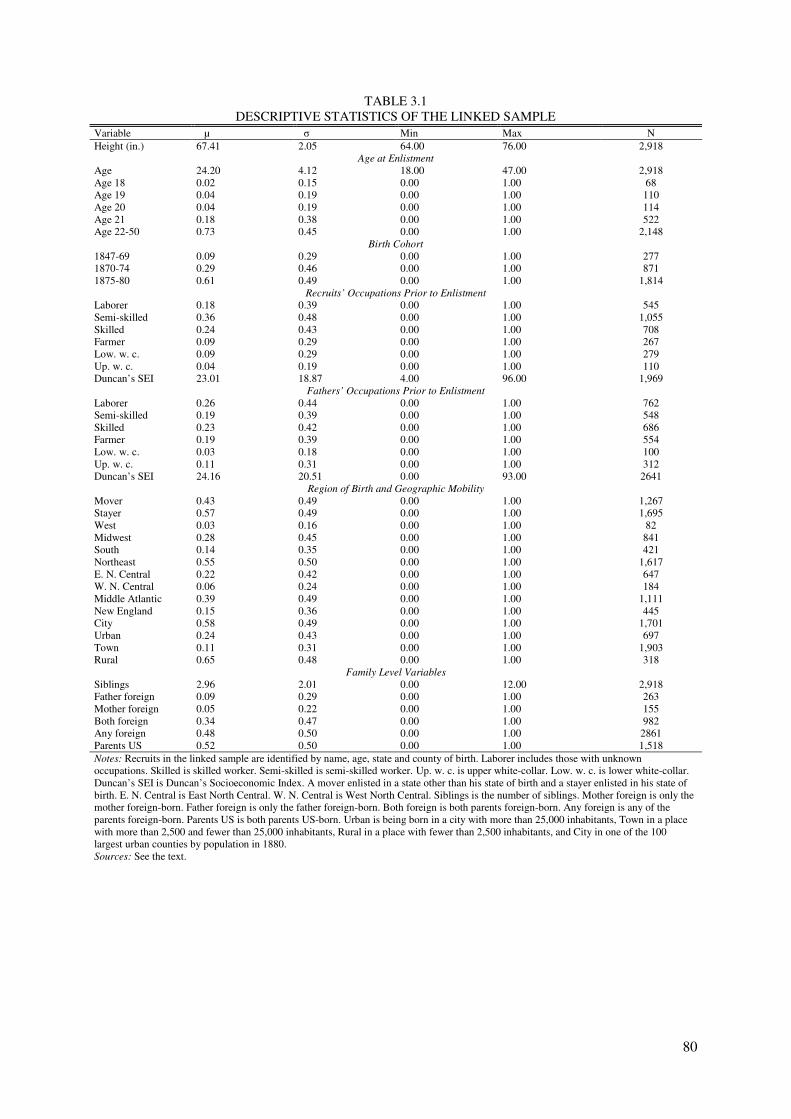
80

TABLE 3.1 DESCRIPTIVE STATISTICS OF THE LINKED SAMPLE

Variable µ σ Min Max N Height (in.) 67.41 2.05 64.00 76.00 2,918

Age at Enlistment

Age 24.20 4.12 18.00 47.00 2,918 Age 18 0.02 0.15 0.00 1.00 68 Age 19 0.04 0.19 0.00 1.00 110 Age 20 0.04 0.19 0.00 1.00 114 Age 21 0.18 0.38 0.00 1.00 522 Age 22-50 0.73 0.45 0.00 1.00 2,148

Birth Cohort

1847-69 0.09 0.29 0.00 1.00 277 1870-74 0.29 0.46 0.00 1.00 871 1875-80 0.61 0.49 0.00 1.00 1,814

Recruits’ Occupations Prior to Enlistment

Laborer 0.18 0.39 0.00 1.00 545 Semi-skilled 0.36 0.48 0.00 1.00 1,055 Skilled 0.24 0.43 0.00 1.00 708 Farmer 0.09 0.29 0.00 1.00 267 Low. w. c. 0.09 0.29 0.00 1.00 279 Up. w. c. 0.04 0.19 0.00 1.00 110 Duncan’s SEI 23.01 18.87 4.00 96.00 1,969

Fathers’ Occupations Prior to Enlistment

Laborer 0.26 0.44 0.00 1.00 762 Semi-skilled 0.19 0.39 0.00 1.00 548 Skilled 0.23 0.42 0.00 1.00 686 Farmer 0.19 0.39 0.00 1.00 554 Low. w. c. 0.03 0.18 0.00 1.00 100 Up. w. c. 0.11 0.31 0.00 1.00 312 Duncan’s SEI 24.16 20.51 0.00 93.00 2641

Region of Birth and Geographic Mobility Mover 0.43 0.49 0.00 1.00 1,267 Stayer 0.57 0.49 0.00 1.00 1,695 West 0.03 0.16 0.00 1.00 82 Midwest 0.28 0.45 0.00 1.00 841 South 0.14 0.35 0.00 1.00 421 Northeast 0.55 0.50 0.00 1.00 1,617 E. N. Central 0.22 0.42 0.00 1.00 647 W. N. Central 0.06 0.24 0.00 1.00 184 Middle Atlantic 0.39 0.49 0.00 1.00 1,111 New England 0.15 0.36 0.00 1.00 445 City 0.58 0.49 0.00 1.00 1,701 Urban 0.24 0.43 0.00 1.00 697 Town 0.11 0.31 0.00 1.00 1,903 Rural 0.65 0.48 0.00 1.00 318

Family Level Variables Siblings 2.96 2.01 0.00 12.00 2,918 Father foreign 0.09 0.29 0.00 1.00 263 Mother foreign 0.05 0.22 0.00 1.00 155 Both foreign 0.34 0.47 0.00 1.00 982 Any foreign 0.48 0.50 0.00 1.00 2861 Parents US 0.52 0.50 0.00 1.00 1,518 Notes: Recruits in the linked sample are identified by name, age, state and county of birth. Laborer includes those with unknown occupations. Skilled is skilled worker. Semi-skilled is semi-skilled worker. Up. w. c. is upper white-collar. Low. w. c. is lower white-collar. Duncan’s SEI is Duncan’s Socioeconomic Index. A mover enlisted in a state other than his state of birth and a stayer enlisted in his state of birth. E. N. Central is East North Central. W. N. Central is West North Central. Siblings is the number of siblings. Mother foreign is only the mother foreign-born. Father foreign is only the father foreign-born. Both foreign is both parents foreign-born. Any foreign is any of the parents foreign-born. Parents US is both parents US-born. Urban is being born in a city with more than 25,000 inhabitants, Town in a place with more than 2,500 and fewer than 25,000 inhabitants, Rural in a place with fewer than 2,500 inhabitants, and City in one of the 100 largest urban counties by population in 1880. Sources: See the text.

81

3.3 Linkage Process

By means of PASW Statistics 17, we link a sample of 53,198 recruits with about 15.9 million

observations from the 1880 manuscript census. To ensure that our results are more accurate

than many previous ones, we restrict our data set to those recruits whose first name, last name,

state of birth, county of birth, and age in 1880 match data in the census of the same year23. As

an additional precaution, we also estimate regressions with a larger sample, which we linked

by dropping the county-of-birth (but not the state-of-birth) criterion (Tables 3.9 and 3.10).

First, we reduced the census data set to white males born between 1847 and 1880, and

then calculated the age of the recruits in 1880 from their age at enlistment and the date of their

enlistment as recorded in the military records. We excluded duplicates of those recruits who

enlisted more than once, and we eliminated those who could not be identified with sufficient

accuracy by their name, age, state, and county of birth. In the linked sample we used

information from the manuscript census to eliminate recruits who were foreign-born but who

had reported at the time of their enlistment that they were native-born (N=51) and recruits

who had claimed to have more than 21 siblings (N=29).

Like all other historical military data, these are not representative of the entire

population because they are limited not only to men but almost exclusively to lower- and

middle-class ones. Since linking this sample with census data makes it all the less

representative, the linkage procedure itself merits attention. When using name, age, state of

birth, and county of birth, we have a linkage rate of about 5%, defined as the number of

recruits successfully linked with records from the 1880 manuscript census divided by the total

number of recruits in our sample of enlistment records. This linkage rate is lower than those

found in other studies, such as Sunder’s (2007) and Ferrie’s (1996) (38 and 19%,

23 Other studies use phonetic algorithms or allow some leeway regarding self-reported age because of poor numeracy of the

recruits thereby trading of accuracy for greater sample size (Steckel, 1983; Ferrie, 1996).

82

respectively), but when we reduce our linkage criteria to name, age, and state of birth, the rate

increases to 23%. There are many possible reasons for these relatively low linkage rates: for

instance, a recruit’s name may have been misspelled, his age may not have been correctly

recorded, or he may have been living elsewhere than his place of birth at the time of the

census. Other studies have found that the poor, illiterate, and unskilled were less likely than

others’ to be correctly recorded in the census, thereby systematically diminishing the

probability of their being included in our linked sample (Ferrie, 1996). Since we used the

exact age in 1880 calculated from enlistment records to link individuals, those with below-

average numeracy skills were also likely to be underrepresented in the linked sample. To

estimate which individual characteristics influence the linkage probability, we use a probit

model (Table 3.2).

TABLE 3.2 DETERMINANTS OF LINKAGE OF THE CONSCRIPT SAMPLE

WITH THE 1880 MANUSCRIPT CENSUS: PROBIT REGRESSION

(1) (2) (3) (4) Matched with

Census (1=yes,0=no)

Marginal Effects of Model 1

Matched with Census

(1=yes,0=no)

Marginal Effects of Model 3

N

Age -0.004** -0.00 Mover -0.13*** -0.01 -0.13*** -0.01 27,984 Stayer Ref. Ref. Ref. Ref. 25,214 Laborer -0.18*** -0.02 -0.18*** -0.02 10,957 Semi-skilled -0.12*** -0.01 -0.12*** -0.01 19,849 Skilled -0.06* -0.01 -0.07** -0.01 10,728 Farmer -0.09** -0.01 -0.09** -0.01 6,327 Low. w. c. Ref. Ref. Ref. Ref. 3,873 Up. w. c. 0.06 0.01 0.05 0.00 1,500 West 0.13** 0.02 0.13** 0.01 1,120 Midwest Ref. Ref. Ref. Ref. 18,012 South -0.17*** -0.02 -0.17*** -0.02 13,385 Northeast 0.14*** 0.02 0.14*** 0.02 20,608 City 0.31*** 0.04 0.31*** 0.03 20,814 Rural Ref. Ref. Ref. Ref. 32,384 Birth Cohorts

1847-54 -0.65*** -0.04 393 1855-59 -0.28*** -0.02 556 1860-64 -0.35*** -0.03 1,435 1865-69 -0.19*** -0.02 4,756 1870-74 Ref. Ref. 12,981 1875-79 -0.10*** -0.01 29,411 1880 -0.21*** -0.02 3,666 Constant -1.57*** -1.58*** Observations 53,198 53,198 Pseudo-R² 0.03 0.04 Notes: * p < 0.10, ** p < 0.05, *** p < 0.01. Laborer includes those with unknown occupations. Skilled is skilled worker. Semi-skilled is semi-skilled worker. Up. w. c. is upper white-collar. Low. w. c. is lower white-collar. City is being born in one of the 100 largest urban counties by population in 1880. Sources: See the text.

83

With higher age the probability of having moved away from one’s county of birth

increases, and therefore the probability of a successful linkage decreases. A recruit’s

registering in a state other than that of his birth is a measure of his above-average mobility; it

also means that he is less likely to be linked than are those who did not move thus: 1

percentage point less 24 . Comparing recruits’ linkage rates according to occupation, the

probability of being successfully linked is 2 percentage points lower for average laborers and

1 percentage point lower for semi-skilled workers, farmers, and skilled workers compared

with lower-level white-collar workers. Regions, too, are a major factor: Southerners are 2

percentage points less likely to be linked while Northeastern and Western recruits are 2

percentage points more likely to be linked than Midwestern recruits. Being born in one of the

urban counties among the 100 that were the most populous in 1880 gives a recruit a 3-to-4-

percentage-point greater chance of being successfully linked, whereas Wilson and Pope

(2003) find it easier to link rural than urban households. The probability of any of the birth

cohorts’ being linked is between 1 and 4 percentage points below that of the 1870-74 birth

cohort (Table 3.2).

This means that the linked sample slightly better represents urban recruits and those

who were among the less geographically mobile. In addition, those born in the Northeast and

West are overrepresented, whereas the opposite is the case for Southerners. Blue-collar

workers and farmers are underrepresented, yet in absolute terms they compose the largest

group in the linked sample. These examples of discrepancies indicate how difficult it is to

control for the selection bias that arises through the linkage process because the variables used

in the selection equation for the determinants of a successful linkage are also used as

correlates of stature (Wilson and Pope, 2003).

24 All interpretation of binary choice models is done by using marginal effects evaluated at the sample mean of all continuous

independent variables, whereas for binary independent variables the marginal effect is calculated for a discrete change from 0

to 1.

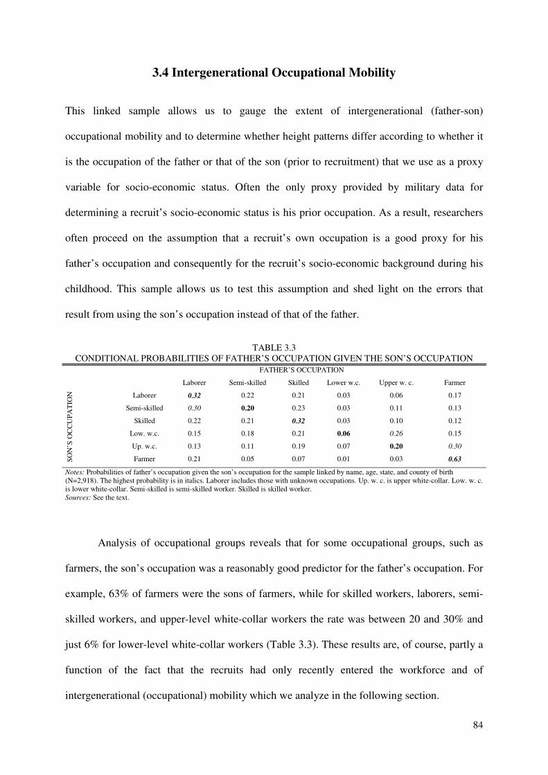
84

3.4 Intergenerational Occupational Mobility

This linked sample allows us to gauge the extent of intergenerational (father-son)

occupational mobility and to determine whether height patterns differ according to whether it

is the occupation of the father or that of the son (prior to recruitment) that we use as a proxy

variable for socio-economic status. Often the only proxy provided by military data for

determining a recruit’s socio-economic status is his prior occupation. As a result, researchers

often proceed on the assumption that a recruit’s own occupation is a good proxy for his

father’s occupation and consequently for the recruit’s socio-economic background during his

childhood. This sample allows us to test this assumption and shed light on the errors that

result from using the son’s occupation instead of that of the father.

TABLE 3.3 CONDITIONAL PROBABILITIES OF FATHER’S OCCUPATION GIVEN THE SON’S OCCUPATION

SO

N’S

OC

CU

PA

TIO

N

FATHER’S OCCUPATION

Laborer Semi-skilled Skilled Lower w.c. Upper w. c. Farmer

Laborer 0.32 0.22 0.21 0.03 0.06 0.17

Semi-skilled 0.30 0.20 0.23 0.03 0.11 0.13

Skilled 0.22 0.21 0.32 0.03 0.10 0.12

Low. w.c. 0.15 0.18 0.21 0.06 0.26 0.15

Up. w.c. 0.13 0.11 0.19 0.07 0.20 0.30

Farmer 0.21 0.05 0.07 0.01 0.03 0.63

Notes: Probabilities of father’s occupation given the son’s occupation for the sample linked by name, age, state, and county of birth (N=2,918). The highest probability is in italics. Laborer includes those with unknown occupations. Up. w. c. is upper white-collar. Low. w. c. is lower white-collar. Semi-skilled is semi-skilled worker. Skilled is skilled worker. Sources: See the text.

Analysis of occupational groups reveals that for some occupational groups, such as

farmers, the son’s occupation was a reasonably good predictor for the father’s occupation. For

example, 63% of farmers were the sons of farmers, while for skilled workers, laborers, semi-

skilled workers, and upper-level white-collar workers the rate was between 20 and 30% and

just 6% for lower-level white-collar workers (Table 3.3). These results are, of course, partly a

function of the fact that the recruits had only recently entered the workforce and of

intergenerational (occupational) mobility which we analyze in the following section.

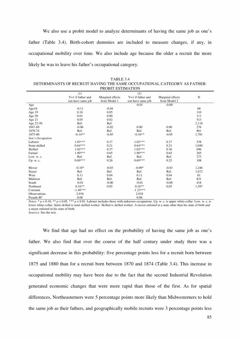
85

We also use a probit model to analyze determinants of having the same job as one’s

father (Table 3.4). Birth-cohort dummies are included to measure changes, if any, in

occupational mobility over time. We also include age because the older a recruit the more

likely he was to leave his father’s occupational category.

TABLE 3.4 DETERMINANTS OF RECRUIT HAVING THE SAME OCCUPATIONAL CATEGORY AS FATHER:

PROBIT ESTIMATION (1) (2) Y=1 if father and

son have same job Marginal effects

from Model 1 Y=1 if father and son have same job

Marginal effects from Model 2

N

Age -0.01 -0.00 Age18 -0.11 -0.04 68 Age 19 0.16 0.05 110 Age 20 0.01 0.00 111 Age 21 0.05 0.02 513 Age 22-50 Ref. Ref. 2,118 1847-69 -0.06 -0.02 0.00 0.00 276 1870-74 Ref. Ref. Ref. Ref. 861 1875-80 -0.14** -0.05 -0.16** -0.05 1,781 Son’s Occupation Laborer 1.03*** 0.37 1.02*** 0.37 538 Semi-skilled 0.64*** 0.21 0.64*** 0.21 1,040 Skilled 1.02*** 0.37 1.02*** 0.36 696 Farmer 1.90*** 0.65 1.90*** 0.65 265 Low. w. c. Ref. Ref. Ref. Ref. 273 Up. w. c. 0.69*** 0.26 0.69*** 0.25 108 Mover -0.10* -0.03 -0.09* -0.03 1,246 Stayer Ref. Ref. Ref. Ref. 1,672 West 0.11 0.04 0.11 0.04 81 Midwest Ref. Ref. Ref. Ref. 831 South -0.01 -0.00 -0.01 -0.00 418 Northeast 0.16** 0.05 0.16** 0.05 1,587 Constant -1.48*** -1.23*** Observations 2,918 2,918 Pseudo-R² 0.08 0.08 Notes: * p < 0.10, ** p < 0.05, *** p < 0.01. Laborer includes those with unknown occupations. Up. w. c. is upper white-collar. Low. w. c. is lower white-collar. Semi-skilled is semi-skilled worker. Skilled is skilled worker. A mover enlisted in a state other than his state of birth and a stayer enlisted in his state of birth. Sources: See the text.

We find that age had no effect on the probability of having the same job as one’s

father. We also find that over the course of the half century under study there was a

significant decrease in this probability: five percentage points less for a recruit born between

1875 and 1880 than for a recruit born between 1870 and 1874 (Table 3.4). This increase in

occupational mobility may have been due to the fact that the second Industrial Revolution

generated economic changes that were more rapid than those of the first. As for spatial

differences, Northeasterners were 5 percentage points more likely than Midwesterners to hold

the same job as their fathers, and geographically mobile recruits were 3 percentage points less

86

likely to do so than those who enlisted in their state of birth. These results corroborate the

pattern reported in Table 3.3: Farmers were most likely to hold the same jobs as their fathers

(by 65 percentage points), followed by laborers and skilled workers (by 37 percentage points),

upper-level white-collar workers (by 26 percentage points), and semi-skilled workers (by 21

percentage points) compared with lower-level white-collar workers (Table 3.4, Model 1).

We use Duncan’s SEI of fathers and sons to examine the correlation between their SEI

scores: an analysis similar to that of intergenerational income inequality or mobility (Becker

and Tomes, 1986; Solon, 1992). We include age at enlistment to control for potential work

experience (Mincer, 1958). Geographic mobility may have had an impact on SEI, but - since

we define a mover simply as a recruit who enlisted elsewhere than in his birth state - we

cannot determine whether it was he or his father who made the decision to move. Perhaps

movers were more willing than others to take risks, their motivation being to improve their

lot; in this case, one would assume that their SEI scores were higher than average. We control

for the nativity of the recruits’ parents to determine whether it had a negative effect on the

recruits’ socio-economic status even when we control for the socio-economic status of their

fathers. We also include the height of the recruits as an independent variable (Table 3.5,

Model 2) to determine whether height was associated with own SEI when controlling for the

fathers’ SEI. Finally, we test whether a recruit’s own or his father’s SEI influenced his height

(Table 3.5, Models 3 and 4).

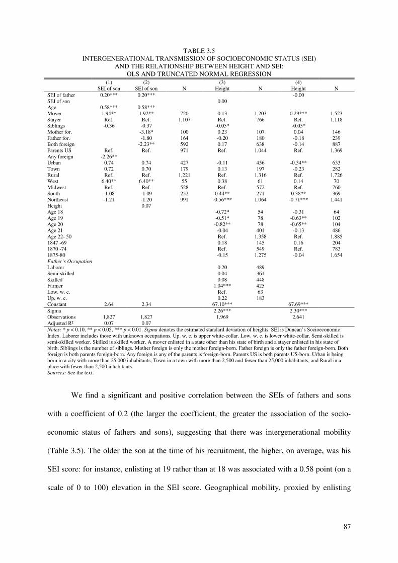
87

TABLE 3.5 INTERGENERATIONAL TRANSMISSION OF SOCIOECONOMIC STATUS (SEI)

AND THE RELATIONSHIP BETWEEN HEIGHT AND SEI: OLS AND TRUNCATED NORMAL REGRESSION

(1) (2) (3) (4) SEI of son SEI of son N Height N Height N SEI of father 0.20*** 0.20*** -0.00 SEI of son 0.00 Age 0.58*** 0.58*** Mover 1.94** 1.92** 720 0.13 1,203 0.29*** 1,523 Stayer Ref. Ref. 1,107 Ref. 766 Ref. 1,118 Siblings -0.36 -0.37 -0.05* -0.05* Mother for. -3.18* 100 0.23 107 0.04 146 Father for. -1.80 164 -0.20 180 -0.18 239 Both foreign -2.23** 592 0.17 638 -0.14 887 Parents US Ref. Ref. 971 Ref. 1,044 Ref. 1,369 Any foreign -2.26** Urban 0.74 0.74 427 -0.11 456 -0.34** 633 Town 0.72 0.70 179 0.13 197 -0.23 282 Rural Ref. Ref. 1,221 Ref. 1,316 Ref. 1,726 West 6.40** 6.40** 55 0.38 61 0.14 70 Midwest Ref. Ref. 528 Ref. 572 Ref. 760 South -1.08 -1.09 252 0.44** 271 0.38** 369 Northeast -1.21 -1.20 991 -0.56*** 1,064 -0.71*** 1,441 Height 0.07 Age 18 -0.72* 54 -0.31 64 Age 19 -0.51* 78 -0.63** 102 Age 20 -0.82** 78 -0.65** 104 Age 21 -0.04 401 -0.13 486 Age 22- 50 Ref. 1,358 Ref. 1,885 1847 -69 0.18 145 0.16 204 1870 -74 Ref. 549 Ref. 783 1875-80 -0.15 1,275 -0.04 1,654 Father’s Occupation

Laborer 0.20 489 Semi-skilled 0.04 361 Skilled 0.08 448 Farmer 1.04*** 425 Low. w. c. Ref. 63 Up. w. c. 0.22 183 Constant 2.64 2.34 67.10*** 67.69*** Sigma 2.26*** 2.30*** Observations 1,827 1,827 1,969 2,641 Adjusted R² 0.07 0.07 Notes: * p < 0.10, ** p < 0.05, *** p < 0.01. Sigma denotes the estimated standard deviation of heights. SEI is Duncan’s Socioeconomic Index. Laborer includes those with unknown occupations. Up. w. c. is upper white-collar. Low. w. c. is lower white-collar. Semi-skilled is semi-skilled worker. Skilled is skilled worker. A mover enlisted in a state other than his state of birth and a stayer enlisted in his state of birth. Siblings is the number of siblings. Mother foreign is only the mother foreign-born. Father foreign is only the father foreign-born. Both foreign is both parents foreign-born. Any foreign is any of the parents is foreign-born. Parents US is both parents US-born. Urban is being born in a city with more than 25,000 inhabitants, Town in a town with more than 2,500 and fewer than 25,000 inhabitants, and Rural in a place with fewer than 2,500 inhabitants. Sources: See the text.

We find a significant and positive correlation between the SEIs of fathers and sons

with a coefficient of 0.2 (the larger the coefficient, the greater the association of the socio-

economic status of fathers and sons), suggesting that there was intergenerational mobility

(Table 3.5). The older the son at the time of his recruitment, the higher, on average, was his

SEI score: for instance, enlisting at 19 rather than at 18 was associated with a 0.58 point (on a

scale of 0 to 100) elevation in the SEI score. Geographical mobility, proxied by enlisting

88

outside the state of birth, was associated with a 2-point increase in the SEI (Table 3.5, Models

1 and 2).

Even when we controlled for the father’s SEI score, having foreign-born parents

translated into a 2.2-point lower score. Having a foreign-born mother but a native-born father

was associated with an even greater difference, as much as 3.2 points25 (Table 3.5, Models 1

and 2): a pattern consistent with the intergenerational persistence of occupations and therefore

of socio-economic status. In contrast, we find no significant correlation either between one’s

height and one’s SEI (Table 3.5, Model 2) or between a son’s height and his father’s SEI

(Table 3.5, Models 3 and 4).

3.5 Re-estimating the Occupational Height Premiums

The linked sample allows us to estimate height differentials by socio-economic status using

the occupation of the father rather than that of the recruit and to investigate the differentials.

When Lantzsch and Schuster (2009) did this, in their study of 19th-century Bavarian

conscripts, they found that the tallest were the sons of farmers, upper-level white-collar

workers, and public officials and that the shortest were the sons of laborers, blue-collar

workers, and apprentices. As for the correlation between the recruit’s own occupation and his

height, they found the same correlation: the shortest had blue-collar jobs, the tallest white-

collar ones.

Our results indicate that using the recruit’s, as opposed to his father’s, occupation

accounts for a certain inaccuracy in estimated heights, but one that is very small; nor does

constraining the standard deviation to 2.7 in. (6.86 cm) substantially alter the results. We find

25 Including the mother’s socioeconomic status proved to be insignificant and did not change the results in Table 3.5.

89

that controlling for the recruit’s occupation translates into a significant height penalty for

skilled workers, whereas controlling for the father’s occupation translates into a significant

height premium for farmers’ sons (Table 3.6, Models 1 and 2). When both the father’s and the

son’s occupations are considered, being a farmer’s son offers the greatest height advantage

(Table 3.6, Model 3). Thus those who entered the farming sector, being on average less well

nourished and therefore shorter than those born in it, must have lowered the average heights

therein. That farmers enjoyed a height premium (an idea substantiated by many studies of the

19th-century US) is in line with Komlos’s (1987) propinquity hypothesis, because this height

premium remains significant even when we control for the size and socio-economic status of

the recruit’s family and his parents’ birth status (foreign or native) (Table 3.8). It follows that

sons of farmers who became upper-level white-collar workers were the tallest and that sons of

semi-skilled workers who became skilled workers were the shortest (Tables 3.6 and 3.7).

Evidently only the tallest from each occupational category entered white-collar occupations,

perhaps because they were also the best educated. Previous studies have failed to link recruits

with family-level data; this study fills that gap in showing that coefficients for birth cohorts

and regions have identical signs and significance, with only minor differences in magnitude

when controlling for the son’s rather than the father’s occupation (Table 3.6).

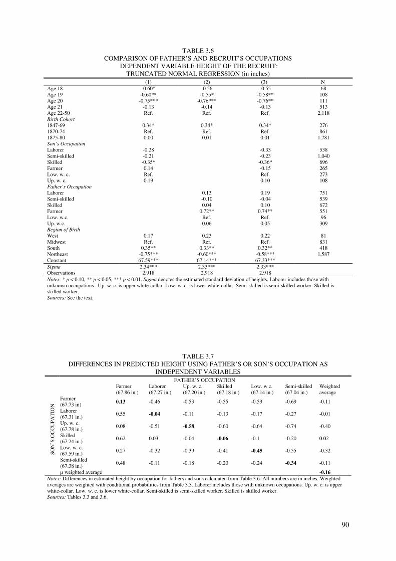
90

TABLE 3.6 COMPARISON OF FATHER’S AND RECRUIT’S OCCUPATIONS

DEPENDENT VARIABLE HEIGHT OF THE RECRUIT: TRUNCATED NORMAL REGRESSION (in inches)

(1) (2) (3) N Age 18 -0.60* -0.56 -0.55 68 Age 19 -0.60** -0.55* -0.58** 108 Age 20 -0.75*** -0.76*** -0.76** 111 Age 21 -0.13 -0.14 -0.13 513 Age 22-50 Ref. Ref. Ref. 2,118 Birth Cohort

1847-69 0.34* 0.34* 0.34* 276 1870-74 Ref. Ref. Ref. 861 1875-80 0.00 0.01 0.01 1,781 Son’s Occupation

Laborer -0.28 -0.33 538 Semi-skilled -0.21 -0.23 1,040 Skilled -0.35* -0.36* 696 Farmer 0.14 -0.15 265 Low. w. c. Ref. Ref. 273 Up. w. c. 0.19 0.10 108 Father’s Occupation

Laborer 0.13 0.19 751 Semi-skilled -0.10 -0.04 539 Skilled 0.04 0.10 672 Farmer 0.72** 0.74** 551 Low. w.c. Ref. Ref. 96 Up. w.c. 0.06 0.05 309 Region of Birth West 0.17 0.23 0.22 81 Midwest Ref. Ref. Ref. 831 South 0.35** 0.33** 0.32** 418 Northeast -0.75*** -0.60*** -0.58*** 1,587 Constant 67.59*** 67.14*** 67.33*** Sigma 2.34*** 2.33*** 2.33*** Observations 2,918 2,918 2,918 Notes: * p < 0.10, ** p < 0.05, *** p < 0.01. Sigma denotes the estimated standard deviation of heights. Laborer includes those with unknown occupations. Up. w. c. is upper white-collar. Low. w. c. is lower white-collar. Semi-skilled is semi-skilled worker. Skilled is skilled worker. Sources: See the text.

TABLE 3.7 DIFFERENCES IN PREDICTED HEIGHT USING FATHER’S OR SON’S OCCUPATION AS

INDEPENDENT VARIABLES

FATHER’S OCCUPATION

SO

N’S

OC

CU

PA

TIO

N

Farmer (67.86 in.)

Laborer (67.27 in.)

Up. w. c. (67.20 in.)

Skilled (67.18 in.)

Low. w.c. (67.14 in.)

Semi-skilled (67.04 in.)

Weighted average

Farmer (67.73 in)

0.13 -0.46 -0.53 -0.55 -0.59 -0.69 -0.11

Laborer (67.31 in.)

0.55 -0.04 -0.11 -0.13 -0.17 -0.27 -0.01

Up. w. c. (67.78 in.)

0.08 -0.51 -0.58 -0.60 -0.64 -0.74 -0.40

Skilled (67.24 in.)

0.62 0.03 -0.04 -0.06 -0.1 -0.20 0.02

Low. w. c. (67.59 in.)

0.27 -0.32 -0.39 -0.41 -0.45 -0.55 -0.32

Semi-skilled (67.38 in.)

0.48 -0.11 -0.18 -0.20 -0.24 -0.34 -0.11

µ weighted average -0.16

Notes: Differences in estimated height by occupation for fathers and sons calculated from Table 3.6. All numbers are in inches. Weighted averages are weighted with conditional probabilities from Table 3.3. Laborer includes those with unknown occupations. Up. w. c. is upper white-collar. Low. w. c. is lower white-collar. Semi-skilled is semi-skilled worker. Skilled is skilled worker. Sources: Tables 3.3 and 3.6.

91

We compare differences in predicted heights by occupation (using the coefficients

estimated in Table 3.6), between using the occupation of the father and that of the recruit

(Table 3.7 and Figure 3.1). For the two occupations associated with the shortest heights (when

the recruit’s occupation is used), those of laborers and skilled workers, estimates were

virtually identical. While upper-level white-collar workers were taller than farmers (when the

recruit’s occupation is used), sons of farmers were taller than sons of lower-level white-collar

workers. Having an upper-level white-collar father was associated with approximately the

same height as having a father who was a lower-level white-collar or skilled worker (Figure

3.1). For recruits who were white-collar workers heights are overestimated by no more than

about 0.5% and for semi-skilled workers, farmers, and laborers by even less (Table 3.7). The

(weighted) average error when using the son’s occupation rather than that of his father is

-0.16 in. (-0.4 cm), implying that occupational height premiums are on average overestimated

by 0.16 in. (0.4 cm) when the son’s, and not the father’s, occupation is used (Table 3.7). The

largest absolute differences in height when controlling, instead, for the father’s occupation are

between upper-level white-collar workers whose fathers were semi-skilled workers and

skilled workers whose fathers were farmers: -0.74 in. (-1.9 cm) and 0.62 in. (1.6 cm). The two

largest (weighted) average differences are overestimations: 0.40 in. (1.0 cm) for upper-level

white-collar sons and 0.32 in. (0.8 cm) for lower-level white-collar sons26 (Table 3.7).

26 However, these results may not be true for all samples.

92

FIGURE 3.1 ESTIMATED HEIGHTS BY FATHER’S AND SON’S OCCUPATION

66,6

66,8

67,0

67,2

67,4

67,6

67,8

68,0

Up. w.c. Farmer Low. w.c. Semi-skilled Laborer Skilled

Inch

es

Son

Father

Notes: Estimated heights from Tables 3.6 and 3.7. Son is recruit’s occupation prior to enlistment. Father is father’s occupation from 1880 manuscript census. Up. w. c. is upper white-collar. Low. w. c. is lower white-collar. Semi-skilled is semi-skilled worker. Skilled is skilled worker. Laborer includes those with unknown occupations. Sources: Tables 3.6 and 3.7.

3.6 Family-Level Correlates of Height

Family-level correlates of height reveal that the number of siblings in a household was

negatively associated with a recruit’s height, whereas foreign-born parents conveyed no

height penalty. The number of siblings had a significant and negative association with height

at the national level, in rural areas, and in the Midwest, but not in urban areas. The effect was

fairly small: an additional child in the household would decrease average height by between

0.05 (0.1 cm) and 0.09 in. (0.2 cm) (Tables 3.8 and 3.9): results similar to Costa’s (1993).

That there was no association with height if either of the parents was foreign-born confirms

Costa’s (1993) and Wilson and Pope’s (2003) findings for the antebellum period. This

suggests that in the US the intergenerational transmission of shorter stature was offset through

relatively high living standards (Tables 3.8 and 3.9). Komlos (2008), using data on US Army

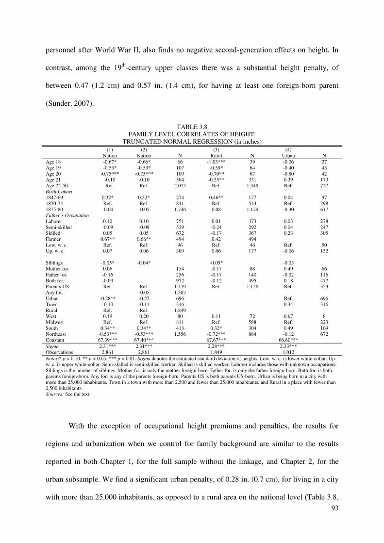
93

personnel after World War II, also finds no negative second-generation effects on height. In

contrast, among the 19th-century upper classes there was a substantial height penalty, of

between 0.47 (1.2 cm) and 0.57 in. (1.4 cm), for having at least one foreign-born parent

(Sunder, 2007).

TABLE 3.8 FAMILY LEVEL CORRELATES OF HEIGHT:

TRUNCATED NORMAL REGRESSION (in inches) (1) (2) (3) (4) Nation Nation N Rural N Urban N Age 18 -0.67* -0.66* 66 -1.03*** 39 -0.06 27 Age 19 -0.53* -0.53* 107 -0.59* 64 -0.40 43 Age 20 -0.75*** -0.75*** 109 -0.70** 67 -0.80 42 Age 21 -0.10 -0.10 504 -0.35** 331 0.39 173 Age 22-50 Ref. Ref. 2,075 Ref. 1,348 Ref. 727 Birth Cohort

1847-69 0.32* 0.32* 274 0.46** 177 0.04 97 1870-74 Ref. Ref. 841 Ref. 543 Ref. 298 1875-80 -0.04 -0.05 1,746 0.08 1,129 -0.30 617 Father’s Occupation

Laborer 0.10 0.10 751 0.01 473 0.03 278 Semi-skilled -0.09 -0.09 539 -0.24 292 0.04 247 Skilled 0.05 0.05 672 -0.17 367 0.23 305 Farmer 0.67** 0.66** 494 0.42 494 Low. w. c. Ref. Ref. 96 Ref. 46 Ref. 50 Up. w. c. 0.07 0.06 309 0.06 177 -0.06 132

Siblings -0.05* -0.04* -0.05* -0.03 Mother for. 0.06 154 -0.17 88 0.49 66 Father for. -0.16 256 -0.17 140 -0.02 116 Both for. -0.03 972 -0.12 495 0.18 477 Parents US Ref. Ref. 1,479 Ref. 1,126 Ref. 353 Any for. -0.05 1,382 Urban -0.28** -0.27 696 Ref. 696 Town -0.10 -0.11 316 0.34 316 Rural Ref. Ref. 1,849 West 0.19 0.20 80 0.11 72 0.67 8 Midwest Ref. Ref. 811 Ref. 588 Ref. 223 South 0.34** 0.34** 413 0.32* 304 0.49 109 Northeast -0.53*** -0.53*** 1,556 -0.72*** 884 -0.12 672 Constant 67.39*** 67.40*** 67.67*** 66.60*** Sigma 2.31*** 2.31*** 2.28*** 2.33*** Observations 2,861 2,861 1,849 1,012 Notes:* p < 0.10, ** p < 0.05, *** p < 0.01. Sigma denotes the estimated standard deviation of heights. Low. w. c. is lower white-collar. Up. w. c. is upper white-collar. Semi-skilled is semi-skilled worker. Skilled is skilled worker. Laborer includes those with unknown occupations. Siblings is the number of siblings. Mother for. is only the mother foreign-born. Father for. is only the father foreign-born. Both for. is both parents foreign-born. Any for. is any of the parents foreign-born. Parents US is both parents US-born. Urban is being born in a city with more than 25,000 inhabitants, Town in a town with more than 2,500 and fewer than 25,000 inhabitants, and Rural in a place with fewer than 2,500 inhabitants. Sources: See the text.

With the exception of occupational height premiums and penalties, the results for

regions and urbanization when we control for family background are similar to the results

reported in both Chapter 1, for the full sample without the linkage, and Chapter 2, for the

urban subsample. We find a significant urban penalty, of 0.28 in. (0.7 cm), for living in a city

with more than 25,000 inhabitants, as opposed to a rural area on the national level (Table 3.8,

94

Model 1). In the Midwest the penalty for living in a town was 0.66 in. (1.7 cm) (Table 3.9,

Model 3). These urban penalties are comparable with the results reported in Chapter 2, where

we find an urban penalty of 0.58 in. (1.5 cm) for being born in one of the ten largest urban

areas in 1880 (population 1,206,299 – 216,090) and a penalty of 0.34 in. (0.9 cm) for being

born in one of the next 90 urban areas (population 160,146 – 19,743) as opposed to a rural

area27 (Table 2.2, Model 2).

We find only sons of farmers at the national level (Table 3.8, Models 1 and 2) to be

about 0.67 in. (1.7 cm) taller than sons of lower-level white-collar workers; as for the other

occupational groups in this sample, there was no significant correlation with stature. As we

reported in Chapter 1, there were significant height premiums both for recruits who were

farmers prior to their recruitment, of 0.30 in. (0.8 cm), and for upper-level white-collar

workers, of 0.22 in. (0.6 cm), and there were significant height penalties both for laborers, of

0.21 in. (0.5 cm), and for skilled workers, of 0.12 in. (0.3 cm), relative to lower-level white-

collar workers (Table 1.10, Model 3).

Growing up in the South conveyed a height premium of about 0.34 in. (0.9 cm),

whereas growing up in the Northeast was associated with a height penalty of between 0.53

(1.3 cm) and 0.72 in. (1.8 cm), relative to the Midwest (Table 3.8). As for regions within the

Midwest, living in the East North Central rather than in the West North Central census

division was associated with a height penalty of 0.41 in. (1.0 cm) (Table 3.9). The results

reported in Chapter 1 are almost identical: a height premium of 0.29 in. (0.7 cm) for

Southerners and a height penalty of 0.73 in. (1.9 cm) for Northeasterners. In Chapter 1 the

height penalty for living in the East North Central rather than the West North Central division

was reported to be 0.18 in. (0.5 cm) (Table 1.3, Models 1 and 2). In the much larger sample of

27 The magnitude of the penalties differs because the definition of rural in this study is a place with less than 2,500 inhabitants, whereas it is

a county with towns of less than 19, 743 inhabitants in Chapter 2.

95

those linked only according to name, age, and state of birth the results are similar, but the

height premium for farmers at the national level becomes insignificant (Table 3.10, Model 1).

TABLE 3.9 FAMILY LEVEL CORRELATES OF HEIGHT BY REGION,

TRUNCATED NORMAL REGRESSION (in inches) (1) (2) (3) (4) Northeast

(County) N Northeast

(State) N Midwest

(County) N Midwest

(State) N

Age 18 -0.73 40 -0.64** 138 -0.38 16 -0.76** 78 Age 19 -0.42 59 -0.68*** 199 -0.22 29 -0.38* 110 Age 20 -0.74* 62 -0.75*** 192 -0.70 31 -0.31 134 Age 21 -0.16 273 -0.04 1,194 -0.02 154 -0.11 811 Age 22-50 Ref. 1,153 Ref. 4,014 Ref. 601 Ref. 2,531 1847-69 0.23 167 0.14 753 0.72** 60 0.35** 445 1870-74 Ref. 459 Ref. 1,538 Ref. 258 Ref. 935 1875-80 0.06 961 -0.07 3,446 -0.18 513 0.03 2,284 Laborer -0.17 455 -0.30 1,876 0.21 175 -0.00 811 Semi-skilled -0.22 402 -0.28 1,233 0.02 100 -0.14 338 Skilled -0.26 427 -0.24 1,414 0.45 156 -0.13 558 Farmer 0.34 86 -0.07 630 0.63 280 0.02 1,596 Low. w. c. Ref. 61 Ref. 157 Ref. 18 Ref. 59 Up. w. c. -0.28 156 0.05 427 0.26 102 0.11 302 Siblings -0.05 -0.03 -0.09* -0.03 Mother for. 0.07 105 -0.18 307 0.11 31 -0.07 116 Father for. -0.03 154 -0.28** 582 -0.06 69 0.14 317 Parents for. 0.11 726 -0.02 2,428 -0.02 189 -0.08 707 Parents US Ref. 602 Ref. 2,420 Ref. 542 Ref. 2,524 Urban -0.14 515 -0.13 1,238 -0.50 99 -0.22 341 Town 0.38 159 0.01 678 -0.66** 124 -0.43*** 381 Rural Ref. 913 Ref. 3,821 Ref. 604 Ref. 2,942 N. England 0.19 454 0.27*** 1,318 M. Atlantic Ref. 1,133 Ref. 4,419 East N. C. -0.41* 647 -0.17* 2,626 West N. C. Ref. 184 Ref. 1,038 Constant 66.74*** 66.97*** 67.87*** 67.75*** Sigma 2.41*** 2.32*** 2.22*** 2.25*** Observations 1,587 5,737 831 3,664 Notes: * p < 0.10, ** p < 0.05, *** p < 0.01. Sigma denotes the estimated standard deviation of heights. County is linked by name, age, state, and county. State is linked by name, age, and state. Up. w. c. is upper white-collar. Low. w. c. is lower white-collar. Semi-skilled is semi-skilled worker. Skilled is skilled worker. Laborer includes those with unknown occupations. A mover enlisted in a state other than his state of birth and a stayer enlisted in his state of birth. Siblings is the number of siblings. Mother for. is only the mother foreign-born. Father for. is only the father foreign-born. Parents for. is both parents foreign-born. Parents US is both parents US-born. Urban is being born in a city with more than 25,000 inhabitants, Town in a town with more than 2,500 and fewer than 25,000 inhabitants, and Rural in a place with fewer than 2,500 inhabitants. N. England is New England. M. Atlantic is Middle Atlantic. East N. C. is East North Central. West N. C. is West North Central. Sources: See the text.

96

TABLE 3.10 FAMILY LEVEL CORRELATES OF HEIGHT: LINKAGE BY NAME, AGE, AND STATE;

TRUNCATED NORMAL REGRESSION (in inches) (1) (2) (3) Nation N Rural N Urban N Age 18 -0.64*** 270 -0.73*** 211 -0.42 59 Age 19 -0.56*** 406 -0.58*** 296 -0.48* 110 Age 20 -0.56*** 414 -0.57*** 312 -0.54 102 Age 21 -0.05 2,562 -0.11 1,973 0.17 589 Age 22-50 Ref. 8,401 Ref. 6,401 Ref. 2,000 1847-69 0.20** 1,504 0.18* 1,154 0.27 350 1870-74 Ref. 3,147 Ref. 2,367 Ref. 780 1875-80 -0.02 7,402 0.03 5,672 -0.18 1,730 Laborer -0.10 3,332 -0.05 2,481 -0.28 851 Semi-skilled -0.15 1,690 -0.20 1,017 -0.11 406 Skilled -0.11 2,246 -0.11 1,371 -0.13 506 Farmer 0.09 3,653 0.10 3,643 0.28 10 Low. w. c. Ref. 255 Ref. 135 Ref. 120 Up. w. c. 0.13 877 0.16 546 0.06 331 Siblings -0.03* -0.04* -0.01 Mother for. -0.10 458 -0.12 291 -0.04 167 Father for. -0.08 992 -0.08 647 -0.05 345 Parents for. -0.03 3,290 0.01 1,978 -0.09 1,303 Parents US Ref. 7,313 Ref. 6,268 Ref. 1,045 Urban -0.17** 1,705 Ref. 1,705 Town -0.19** 1,155 -0.01 1,155 Rural Ref. 9,193 West 0.01 180 -0.04 165 0.50 15 Midwest Ref. 3,664 Ref. 2,942 Ref. 722 South 0.31*** 2,472 0.32*** 2,264 0.13 208 Northeast -0.74*** 5,736 -0.81*** 3,821 -0.54*** 1,915 Constant 67.60*** 67.60*** 67.38*** Sigma 2.33*** 2.33*** 2.29*** Observations 12,053 9,193 2,860 Notes: * p < 0.10, ** p < 0.05, *** p < 0.01. Sigma denotes the estimated standard deviation of heights. Up. w. c. is upper white-collar. Low. w. c. is lower white-collar. Semi-skilled is semi-skilled worker. Skilled is skilled worker. Laborer includes those with unknown occupations. A mover enlisted in a state other than his state of birth and a stayer enlisted in his state of birth. Siblings is the number of siblings. Mother for. is only the mother foreign-born. Father for. is only the father foreign-born. Parents for. is both parents foreign-born. Parents US is both parents US-born. Urban is being born in a city with more than 25,000 inhabitants, Town in a town with more than 2,500 and fewer than 25,000 inhabitants, and Rural in a place with fewer than 2,500 inhabitants. Sources: See the text.

3.7 Conclusion

We find that occupational mobility was increasing during the period under consideration and

that Northeasterners were more likely to have the same occupation as their fathers, whereas

geographic mobility lowered this probability. Sons of farmers were most likely to hold the

same job as their fathers, followed by laborers, skilled workers, upper-level white-collar

workers, and semi-skilled workers relative to lower-level white-collar workers. Using

Duncan’s Socioeconomic Index (SEI), we find a significant and positive correlation between

fathers’ and sons’ SEI scores, implying mobility.

97

We find that when controlling for the son’s instead of the father’s occupation we

overestimate the heights of all occupational categories except for that of skilled workers, but

only by at most 0.5%, or about 0.40 in. (1.0 cm). In the absence of information on the father’s

occupation, the bias that results from using the son’s occupation is small, and the signs and

significance of all other coefficients remain unchanged. This finding will come as good news

to researchers who use the son’s occupation as a proxy for the father’s in anthropometric

studies.

Our analysis of family-level correlates of height reveals that the number of siblings in

a household and an urban place of birth were negatively associated with height, whereas

having a father who was a farmer conveyed a height premium. In the Northeast, family-level

correlates had no significant association with height, whereas being born in the South was

associated with a height premium. Even when we control for family-level variables, all of the

categories with the exception of occupations corroborate the findings described in Chapters 1

and 2. There are only minor differences between the results derived from the large sample of

recruits linked by, among other data, state of birth and those from the small sample linked by

county of birth. Of particular interest are the results indicating that those with foreign-born

parents must have experienced substantial growth: enough to catch up with the average height

of those with native-born parents. Evidently living standards in the US during the second half

of the 19th-century were sufficiently high that it took only one generation to eliminate the

stature discrepancy between newcomers and other Americans.

98

References

Data:

National Archives and Records Administration. 7th and Pennsylvania Ave., NW,

Washington, DC 20408-0001. Microfilm ID M233. Record Group 094. Register of

Enlistments in the U.S. Army, 1798-1914. Vol 94 (96%), Vol 96 (100%), Vol 97(10%), Vol

98 (93%), Vol 100 (88%),Vol 102 (100%), Vol 103 (80%), Vol 104 (100%), Vol 105 (100%).

North Atlantic Population Project and Minnesota Population Center. 2008. NAPP:

Complete Count Microdata. NAPP Version 2.0. Minneapolis, MN: Minnesota Population

Center, 2008. http://www.nappdata.org

Literature:

A’Hearn, Brian. 2004. “A restricted maximum likelihood estimator for truncated height

samples.” Economics and Human Biology, 2: 5-19.

Becker, Gary, and Nigel Tomes. 1986. “Human Capital and the Rise and Fall of Families.”

Journal of Labor Economics, 4 (3): S1-39.

Bodnar, John. 1987. The Transplanted: A History of Immigrants in Urban America.

Bloomington, IN: Indiana University Press.

Costa, Dora. 1993. “Height, Wealth, and Disease among the Native-born in the Rural,

Antebellum North.” Social Science History, 17 (3): 355-383.

Cole, T. J. 2000. “Galton’s midparent height revisited.” Annals of Human Biology, 27 (4):

401-405.

Duncan, Otis D. 1961. “A Socioeconomic Index for All Occupations.” In: Occupations and

Social Status, ed. A. J. Reiss, 109-161. Glencoe, NY: Free Press of Glencoe.

Ferrie, Joseph. 1996. “A New Sample of Males Linked from the Public Use Micro Sample

of the 1850 US Federal Census of Population to the 1860 US Federal Census Manuscript

Schedules.” Historical Methods, 29: 141-156.

Fogel, Robert. 1994. “Economic Growth, Population Theory, and Physiology: the Bearing of

Long-term Processes on the Making of Economic Policy.” American Economic Review, 84:

369–395.

99

Frisancho, Robert A. 1990. Anthropometric Standards for the Assessment of Growth and

Nutritional Status. Ann Arbor: University of Michigan Press.

Haines, Michael, Lee A. Craig, and Thomas Weiss. 2003. “The Short and the Dead:

Nutrition, Mortality, and the ‘Antebellum Puzzle’ in the United States.” Journal of Economic

History, 63: 382-413.

Komlos, John. 1987. “The Height and Weight of West Point Cadets: Dietary Change in

Antebellum America.” The Journal of Economic History, 47: 897-927.

Komlos, John. 2004. “Improvements in Maximum Likelihood Estimators of Truncated

Normal Samples with Prior Knowledge of σ. A Simulation Based Study with Application to

Historical Height Samples.” Discussion Paper LMU Munich.

Komlos, John. 2008. “Stagnation of Heights Among Second-Generation U.S.-Born Army

Personnel.” Social Science Quarterly, 89 (2): 445-455.

Lantzsch, Jana, and Klaus Schuster. 2009. “Socioeconomic status and physical stature in

19th-century Bavaria.” Economics and Human Biology, 7 (1): 46-54.

Lee, Chulhee. 1997. “Socioeconomic Background, Disease, and Mortality among Union

Army Recruits: Implications for Economic and Demographic History.” Explorations in

Economic History, 34: 27-55.

Mincer, Jacob. 1958. “Investment in Human Capital and Personal Income Distribution.” The

Journal of Political Economy, 66 (4): 281-302.

Nam, Charles, and Monica Boyd. 2004. “Occupational Status in 2000; Over a Century of

Census-Based Measurement.” Population Research and Policy Review, 23 (4): 327-358.

Preston, Samuel H., and Michael Haines. 1991. Fatal Years: Child Mortality in the Late

Nineteenth-Century America. Princeton, NJ: Princeton University Press.

Roberts, Evan, Matthew Woollard, Chad Ronnander, Lisa Y. Dillon, and Gunnar

Thorvaldsen. 2003. “Occupational Classification in the North Atlantic Population Project.”

Historical Methods, 36 (2): 89-96.

Sobek, Matthew. 1996. “Work, Status, and Income: Men in the American Occupational

Structure since the Late Nineteenth Century.” Social Science History, 20 (2): 169-207.

Solon, Gary. 1992. “Intergenerational Income Mobility in the United States.” American

Economic Review, 82 (3): 393-408.

Steckel, Richard. 1983. “The economic foundations of East-West migration during the 19th

century.” Explorations in Economic History, 20 (1): 14-36.

100

Steckel, Richard. 1995. “Stature and the Standard of Living.” Journal of Economic

Literature, 33 (4): 1903-1940.

Sunder, Marco. 2007. “Passports and Economic Development: An Anthropometric History

of the U.S. Elite in the Nineteenth Century.” PhD diss. University of Munich.

Wilson, Sven, and Clayne Pope. 2003. “The Height of Union Army Recruits: Family and

Community Influences.” In: Health and Labor Force Participation over the Life Cycle:

Evidence from the Past, ed. Dora Costa, 113-146. Chicago: The University of Chicago Press.

101

Lebenslauf

Matthias Zehetmayer

Geburtsdatum: 10. 3. 1983

Geburtsort: München

Ausbildung

1989-1993 Grundschule Lochhausen 1993-1999 Gymnasium Gröbenzell 1999-2002 Ludwigsgymnasium München 2003-2008 Volkswirtschaftslehre (Diplom)

LMU München Beschäftigung

2009 - 2011 Wissenschaftlicher Mitarbeiter am Seminar für Wirtschaftsgeschichte, LMU München