Estudios Gerenciales 32 (2016) 208–220

ESTUDIOS GERENCIALES

www .e lsev ier .es /es tudios gerenc ia les

Article

An analysis on operational risk in international banking: A Bayesianapproach (2007–2011)

José Francisco Martínez-Sánchez a, María Teresa V. Martínez-Palacios a, Francisco Venegas-Martínezb,∗

a Profesor-Investigador, Escuela Superior de Apan, Universidad Autónoma del Estado de Hidalgo, Apan, Mexicob Profesor-Investigador, Escuela Superior de Economía, Instituto Politécnico Nacional, México D.F., Mexico

a r t i c l e i n f o

Article history:

Received 16 January 2016

Accepted 27 June 2016

Available online 13 September 2016

JEL classification:

D81

C11

C15

Keywords:

Operational risk

Bayesian analysis

Monte Carlo simulation

a b s t r a c t

This study aims to develop a Bayesian methodology to identify, quantify and measure operational risk

in several business lines of commercial banking. To do this, a Bayesian network (BN) model is designed

with prior and subsequent distributions to estimate the frequency and severity. Regarding the subsequent

distributions, an inference procedure for the maximum expected loss, for a period of 20 days, is carried

out by using the Monte Carlo simulation method. The business lines analyzed are marketing and sales,

retail banking and private banking, which all together accounted for 88.5% of the losses in 2011. Data

was obtained for the period 2007–2011 from the Riskdata Operational Exchange Association (ORX), and

external data was provided from qualified experts to complete the missing records or to improve its poor

quality.

© 2016 Universidad ICESI. Published by Elsevier Espana, S.L.U. This is an open access article under the

CC BY license (http://creativecommons.org/licenses/by/4.0/).

Un análisis del riesgo operacional en la banca internacional: un enfoquebayesiano (2007-2011)

Códigos JEL:

D81

C11

C15

Palabras clave:

Riesgo operacional

Análisis bayesiano

Simulación Monte Carlo

r e s u m e n

Esta investigación tiene como propósito desarrollar una metodología bayesiana para identificar, cuan-

tificar y medir el riesgo operacional en distintas líneas de negocio de la banca comercial. Para ello se

disena un modelo de red bayesiana con distribuciones a priori y a posteriori para estimar la frecuencia y

la severidad. Con las distribuciones a posteriori se realiza inferencia sobre la máxima pérdida esperada,

para un período de 20 días, utilizando el método de simulación Monte Carlo. Las líneas de negocio anali-

zadas son comercialización y ventas, banca minorista y banca privada, que en conjunto representaron el

88,5% de las pérdidas en 2011. Los datos fueron obtenidos de la Asociación Riskdata Operacional Exchange

(ORX) para el período 2007-2011, y la información externa fue proporcionada por expertos calificados

para completar los registros faltantes o mejorar los datos de mala calidad.

© 2016 Universidad ICESI. Publicado por Elsevier Espana, S.L.U. Este es un artıculo Open Access bajo la

licencia CC BY (http://creativecommons.org/licenses/by/4.0/).

∗ Corresponding author at: Cerro del Vigía 15, Col. Campestre Churubusco, Del. Coyoacán, 04200 México D.F., Mexico.

E-mail address: fvenegas1111@yahoo.com.mx (F. Venegas-Martínez).

http://dx.doi.org/10.1016/j.estger.2016.06.004

0123-5923/© 2016 Universidad ICESI. Published by Elsevier Espana, S.L.U. This is an open access article under the CC BY license (http://creativecommons.org/licenses/by/4.

0/).

J.F. Martínez-Sánchez et al. / Estudios Gerenciales 32 (2016) 208–220 209

Uma análise do risco operacional no sistema bancário internacional:uma abordagem bayesiana (2007-2011)

Classificac ões JEL:

D81

C11

C15

Palavras-chave:

Risco operacional

Análise bayesiana

Simulac ão de Monte Carlo

r e s u m o

Esta pesquisa tem como objetivo desenvolver uma metodologia Bayesiana para identificar, quantificar e

medir o risco operacional em diversas linhas de negócio da banca comercial. Isso requer (e é projetado)

um modelo de Rede Bayesiana (RB), com distribuic ões anteriores e posteriores para estimar a frequência e

a severidade. Com as distribuic ões posteriores é realizada una inferência sobre a perda máxima esperada

por um período de 20 dias, usando o método de simulac ão de Monte Carlo. As linhas de negócio analisadas

são marketing e vendas, banca de retalho e banca privada, que juntos representaram 88,5% das perdas

em 2011. Os dados foram obtidos a partir da Associac ão Riskdata Operacional Exchange (ORX) para

o período 2007-2011, e a informac ão externa foi fornecida por peritos qualificados para completar os

registros ausentes ou melhorar os dados de má qualidade.

© 2016 Universidad ICESI. Publicado por Elsevier Espana, S.L.U. Este e um artigo Open Access sob uma

licenc a CC BY (http://creativecommons.org/licenses/by/4.0/).

1. Introduction

While in 2004 regulators focused on market, credit and liquid-ity risk, in 2011 attention was mainly placed on the high-profileloss events affecting several major financial institutions, whichrenewed operational risk management and corporate governance.For global markets, the significance of loss events (measured, insome cases, in billions of dollars) showed that the lack of anappropriate operational risk management may affect even majorfinancial institutions.

The current challenge is how to manage proactively operationalrisk in a business environment characterized by sustained volatil-ity. Needless to say financial organizations need advanced tools,models, techniques and methodologies that combine internal datawith external data across industry. For example, organizations inthe banking and insurance sectors can provide critical insightsfrom self-assessment and scenario modeling from the combina-tion of internal data with external data on loss events that triggersacross the industry. External loss event data not only providesinsights from the experiences of industry peers, but also allows amore effective identification of potential risk exposure. For increas-ing effectiveness in analyzing potential risk exposure, predictiveindexes and indicators combining internal and external data maybe developed for a more effective operational risk management.These predictions will lead to a more accurate evaluation of poten-tial future losses.

The Bayesian approach may be an appropriate alternative foroperational risk analysis when initial and/or complementary infor-mation from qualified consultants is available. By construction,Bayesian models incorporate initial or complementary informa-tion about parameter values of a sampling distribution through aprior probability distribution, which includes subjective informa-tion provided by expert opinions, analyst judgments or specialistbeliefs. Subsequently, a posterior distribution is estimated to carryout inference on the parameter values. This paper develops aBayesian Network (BN) model to examine the relationships amongoperational risk (OR) events in the three lines of business withgreater losses in the international banking sector. The proposedBN model is calibrated with observed data from events occurredin these lines of business and/or with information obtained fromexperts or from external sources.1 In this case, experts mainly com-plete missing records or improve data of poor quality. The analysis

1 When referring to experts, they are banking officials who have the experience

and knowledge of the operation and management of the bank business lines.

period for this research is from 2007 to 2011 on the basis of atwenty-day frequency. This period starts one year before the finan-cial crisis generated by subprime mortgages.

OR usually involves a small part of total annual losses fromcommercial banks; however, at the time an extreme event of oper-ational risk occurs, it can cause significant losses. For this reason,major changes in the worldwide banking industry are aimed at hav-ing better policies and recommendations concerning operationalrisk. It is noteworthy that exist in the literature various statisticaltechniques to identify and quantify OR, which have the under-lying assumption of independence between risk events; see, forexample: Degen, Embrechts, and Lambrigger (2007), Moscadelli(2004), Embrechts, Furrer, and Kaufmann (2003). However, asshown in Aquaro et al. (2009), Supatgiat, Kenyon, and Heusler(2006), Carrillo-Menéndez and Suárez-González (2015), Carrillo-Menéndez, Marhuenda-Menéndez, and Suárez-González (2007),Cruz (2002), Cruz, Peters, and Shevchenko (2002), Neil, Marquez,and Fenton (2004) and Alexander (2002) there is a causal relation-ship between OR factors.

Despite the research from Reimer and Neu (2003, 2002), Kartikand Reimer (2007), Aquaro et al. (2009), Neil et al. (2004) andAlexander (2002), that apply the BN scheme in OR management,there is no a complete guide on how to classify, identify, quantify ORevents, and how to calculate economic capital consistently.2 Thiswork aims to close these gaps. First, establishing OR event informa-tion structures so that it is possible to quantify the OR events andthen changing the assumption of independence of events in orderto model more realistically the causality relationship of OR events.

The possibility of using conditional distribution (discrete or con-tinuous), calibrating the model with both objective and subjectiveinformation sources, and establishing causal relationships amongrisk factors, is precisely what distinguishes our research comparedwith classical statistical models. Under this framework, this paper isaimed at calculating, with several confidence levels, the maximumexpected loss over a period of 20 days for the group of internationalbanks associated to the ORX regarding the studied lines of busi-ness of commercial banks, which has to be considered to properlymanage operational risk in ORX.

This paper is organized as follows. Section 2 presents thetypology to be used for OR management in accordance withthe Data Operational Riskdata eXchange Association (ORX). Sec-tion 3, briefly, reviews the main methods, models and tools for

2 Usually, to measure the maximum expected loss (or economic capital) by OR

value it is used the Conditional Value at Risk (CVaR).

210 J.F. Martínez-Sánchez et al. / Estudios Gerenciales 32 (2016) 208–220

measuring OR. Section 4 discusses the theoretical frameworkneeded for the development of this research, emphasizing on theadvantages and benefits of using BNs. Section 5 provides two BN,one for frequency and other for severity. In order to quantify the ORat each node of the network, we fit prior distributions by using the@Risk software. Once the prior probabilities of both networks areestimated, we proceed to calculate posterior probabilities and, sub-sequently, we use the junction tree algorithm to eradicate cycleswhen the directionality is eliminated (See Appendix). Section 6combines prior and posterior distributions to compute the loss dis-tribution by using Monte Carlo simulation. Here, the maximumexpected loss arising from operational risk events for a period of20 days is calculated. Finally, we present conclusions andacknowledge limitations.

2. Operational risk events in the international bankingsector

This section describes, in some detail, the operational risk eventsrelated to the international banking sector according with the DataOperational Riskdata eXchange Association (ORX).

• External frauds

We describe now the operational risk events related to externalfraud according to ORX:a) Fraud and theft: these are losses due to a fraudulent act, misap-

propriate property, or law circumvent, by a third party withoutthe assistance of the bank staff.

b) Security systems: this applies to all events related to unautho-rized access to electronic data files.

• Internal frauds

The operational risk events related to internal fraud aredescribed below:a) Fraud and theft: losses due to fraudulent acts, improper appro-

priations of goods, or evasion of regulation or company policy,that involves the participation of internal staff.

b) Unauthorized activities: losses caused from unreportedintentional and unauthorized operations, or intentionallyunregistered positions.

c) Security systems: this previous category applies to all eventsinvolving unauthorized access to electronic data files for per-sonal profit with the assistance of employee’s access.

• Malicious damage

Losses caused by acts of badness or hatred, in others wordsmalicious damage.a) Deliberate damage: this is concerned with acts of vandalism,

excluding events in security systems.b) Terrorism: ill-intentioned damage caused by terrorist acts

excluding events related to security systems.c) Security systems (external): these events include security

events with deliberate damage in external systems made bya third party without the assistance of internal staff (e.g., thespread of software viruses).

d) Security systems (internal): this includes deliberate events inthe security of internal systems with the participation of inter-nal staff (e.g., the spread of software viruses).

• Labor practices and workplace safety

Labor practices and safety at workplace are losses derivedfrom actions not in agreement with labor, health or safetyregulation. Payment claims for bodily injury or loss of dis-criminatory events. Mandatory insurance programs for workersand regulation on safety in the workplace are included in thiscategory.

• Customers, products and business practice

Business practices, these events consider losses arising from anunintentional or negligent breach of a professional obligation tospecific clients or the design of a product, including fiduciary andsuitability requirements.

• Disasters and accidents

Disasters and accidents reflects losses resulting from damage tophysical assets from natural disasters, or other events like trafficaccidents.

• Technology and infrastructure failure

Losses caused by failures in systems or management.a) Failures in technology and infrastructure, such as hardware,

software and telecommunications malfunctioning.b) Failures in management processes.

3. Operational risk measurement in the internationalbanking sector

Operational risk management usually involves a small part oftotal annual losses from international banks; however, when anunexpected extreme event, that occasionally occurs, may causesignificant losses. For this reason, major changes in the world-wide banking industry are aimed at obtaining better policiesand/or recommendations concerning with operational risk man-agement. Financial globalization and local regulation leads us alsoto rethink and reorganize operational risk associated to interna-tional banking, including those too big to fail. In this sense, asuitable operational management in the international banking sec-tor may avoid possible bankruptcy and contagion and, therefore,systemic risk. The available approaches to deal with this issuevary from simple to highly complex methods with very sophis-ticated statistical models. Now, we briefly describe some of theexisting methods in the literature for measuring OR; see, for exam-ple, Heinrich (2006) and Basel II (2001a, 2001b). It will be alsoemphasized in this subsection on the advantages and benefits ofusing BN.

1) The “top-down” single indicator methods. These methods werechosen by the Basel Committee as a first approach to opera-tional risk measurement. A single indicator of the institution astotal income, volatility of income, or total expenditure, can beconsidered as the functional variable to manage the risk.

2) The “bottom-up” models including expert judgment. The basisfor an expert analysis is a set of scenarios. In this case, expertsmainly complete missing records or improve data of poor qualityof the identified risks and their probabilities of occurrence inalternative scenarios.

3) Internal measurement. The Basel Committee proposes the inter-nal measurement approach as a more advanced method forcalculating the regulatory capital.

4) The classical statistical approach. This framework is similar towhat is used in the quantification methods for market risk, andmore recently the credit risk. However, contrary to what hap-pens with market risk, it is difficult to find a widely acceptedstatistical method.

5) Causal models. As an alternative to the classical statistical frame-work, causal models assume dependence in the occurrenceof OR events. Under this approach, each event represents arandom variable (discrete or continuous) with a conditionaldistribution function. In case that the events have no histori-cal records or data has poor quality, it is required the opinionor judgment of experts to determine the conditional probabil-ities of occurrence. The tool for modeling this causality is justthe BN, which is based on Bayes’ theorem and the networktopology.

J.F. Martínez-Sánchez et al. / Estudios Gerenciales 32 (2016) 208–220 211

4. Theoretical framework for Bayesian network

In this section the theory supporting the development of theproposed BN is presented. It begins with a discussion of the condi-tional value at risk (CVaR) as a coherent risk measure in the senseof Artzner, Delbaen, Eber, and Heath (1999). The CVaR will be usedto compute the expected loss. Afterward, the main concepts of theBN approach are introduced.

Acording to Panjer (2006), the CVaR or Expected Shortfall (ES)is an alternative measure to Value at Risk (VaR) that quantifies thelosses that can be found in the distributions tails. Specifically, let X

be the random variable representing the losses, the CVaR of X witha (1 − p) × 100% confidence level, denoted by CVaR(X), representsthe expected loss given that the total losses exceed the 100 × pquantile of the distribution of X. Thus, CVaRp (X) can be written as:

CVaRp(X) = E[X|X > xp] =

∫ ∞

xpx dF(x)

1 − F(xp)(1)

where F(x) is the cumulative distribution function of X. Hence, theCVaR(X) can be seen as the average of all the values of VaR with a p ×

100% confidence level. Finally, notice that CVaR(X) can be rewrittenas:

CVaRp(X) = E[X|X > xp] = xp +

∫ ∞

xp(x − xp) dF(x)

1 − F(xp)=VaRp(x) + e(xp).

(2)

where e(xp) is the average excess of loss function.3

• The Bayesian framework

In statistical analysis there are two main paradigms, the fre-quentist and the Bayesian. The main difference between them isthe definition of probability. The frequentist states that the prob-ability of an event is the limit of its relative frequency in the longrun. While the Bayesian argue that probability is subjective. Thesubjective probability (degree of belief) is based on knowledgeand experience and is represented through a prior distribution.The subjective beliefs are updated by adding new informationto the sampling distribution through Bayes’ theorem obtaininga posterior distribution, which is used to make inferences onthe parameters of the sampling model. Thus, a Bayesian deci-sion maker learns and revises its beliefs based on new availableinformation.4 Formally, Bayes’ theorem states that

P(�|y) ∝ L(�|y)�(�) (3)

where � is a vector of unknown parameters to be estimated, y isa vector of observations recorded, �(�) is the prior distribution,L(�|y) is the likelihood function for �, and P(�|y) is the posterior

distribution of �. Two main questions arise, how to translate prior

information in an analytical form, �(�), and how to assess thesensitive of the posterior with respect to the prior selection.5

A BN is a graph representing the domain of decision variables,its quantitative and qualitative relations and their probabilities.A BN may also include utility functions that represent the pre-ferences of the decision maker. An important feature of a BN isits graphical form, which allows a visual representation of com-plicated probabilistic reasoning. Another relevant aspect is thequalitative and quantitative parts of a BN, allowing incorporatesubjective elements such as expert opinion. Perhaps the most

3 For a complete analysis on the non coherence of VaR see Venegas-Martínez

(2006).4 For a review of issues associated with Bayes’ theorem see Zellner (1971).5 These questions are a very important topic Bayesian inference; see, in this

regard, Ferguson (1973).

important feature of a BN is that it is a direct representation ofthe real world and not a way of thinking. Each node is associatedwith a set of tables of probabilities in a BN. The nodes stand for therelevant variables, which can be discrete or continuous.6 A causalnetwork according to Pearl (2000) is a BN with the additionalproperty that the “parent” nodes are the directed causes.7

A BN is used primarily for inference by calculating conditionalprobabilities given the information available at each time for eachnode (beliefs). There are two classes of algorithms for the infer-ence process: the first generates an exact solution and the secondproduces an approximate solution with high probability to bein close proximity to the exact solution. Among the exact infer-ence algorithms, we have for example: polytree, clique tree, treejunction, algorithms of variable elimination and Pear’s method.

The use of approximate solutions is based on the exponentialgrowth of the processing time required to obtain exact solutions.According to Guo and Hsu (2002) such algorithms can be groupedin: stochastic simulation methods, model simplification meth-ods, search based methods, and loopy propagation methods. Thebest known is the stochastic simulation, which is, in turn, dividedin sampling algorithms and Markov Chain Monte Carlo (MCMC)methods.

5. Building a Bayesian network for the internationalbanking sector

In what follows, we will be concerned with building the BN forthe international banking sector. The first step is to define the prob-lem domain where the purpose of the NB is specified. Subsequently,the important variables and nodes are defined. Then, the interrela-tionships between nodes and variables are graphically represented.The resulting model must be validated by experts in the field. Incase of disagreement between them, we return to one of the abovesteps until reaching consensus. The last three steps are: incorporateexpert opinion (referred to as the quantification of the network),create plausible scenarios with the network (network applications),and finally network maintenance.

The main problems that a risk manager faces when using a BNare: how to implement a Bayesian network, how to model the struc-ture, how to quantify the network, how to use subjective data (fromexperts) and/or objective (statistical data), what tools should beused for best results, and how to validate the model. The answersto these questions will be addressed in the development of our pro-posal. Moreover, one of the objectives of this paper is to develop aguide for implementing a NB to manage operational risk in inter-national banking associated with ORX. We also seek to generate aconsistent measurement of the minimal capital requirements formanaging OR.

We will be concerned with the analysis of operational risk eventsoccurring in the following lines of business: marketing and sales,retail banking and private banking of international banks joinedto the Operational Riskdata eXchange Association. Once the riskfactors linked with each business line are identified, the nodesthat will be part of the Bayesian network have to be defined.They are random variables that can be discrete or continuous andhave associated probability distributions. One of the purposes ofthis research is to compute the monthly maximum expected loss

6 The following definitions will be needed for the subsequent development of

this research: Definition 1, Bayesian networks are directed acyclic graph (DAGs);

Definition 2, a graph is defined as a set of nodes connected by arcs; Definition 3, if

between each pair of nodes there is a precedence relationship represented by arcs,

then the graph is directed; Definition 4, A cycle is a path that starts and ends at the

same node; and Definition 5, A path is a series of contiguous nodes connected by

directed arcs.7 See Jensen (1996) for a review of the BN theory.

212 J.F. Martínez-Sánchez et al. / Estudios Gerenciales 32 (2016) 208–220

Table 1

Network nodes for severity.

Node Description States (loss D )

Failure in ICT and

disaster

Failure in information

technologies (ICT) and

disaster

0–500

500–1000

1000–1500

1500–2000

2000–2500

2500–3000

More than 3000

People Human mistakes 0–5000

5000–10,000

10,000–15,000

15,000–20,000

20,000–25,000

25,000–30,000

30,000–35,000

More than 35,000

Processes Failure in processes 0–20,000

20,000–40,000

40,000–60,000

60,000–80,000

80,000–100,000

100,000–120,000

120,000–140,000

More than 140,000

Loss (severity) Expected loss for

operational risk events

0–20,000

20,000–40,000

40,000–60,000

60,000–80,000

80,000–100,000

100,000–120,000

More than 120,000

Source: Own elaboration.

associated to transnational banks belonging to ORX. The frequencyof the available data is every twenty days, ranging from 2007through 2011.

• Building and quantifying the model

The nodes are connected with directed arcs (arrows) to forma structure that shows the dependence or causal relationshipbetween them. The BN is divided into two networks, one formodeling the frequency and the other for the severity. Oncethe results are obtained separately, they are aggregated throughMonte Carlo simulation to estimate the loss distribution. Usually,the severity network requires a significant amount of probabil-ity distributions. In what follows, the characteristics and statesof each node of the networks for severity and frequency aredescribed in Tables 1 and 2, respectively.

In the Bayesian approach, the parameters of a sample modelare treated as random variables. The prior knowledge about thepossible values of the parameters is modeled by a specific prior

distribution. Thus, when initial is vague or has little importance auniform, maybe improper, distribution will allow the data speakfor itself. The information and tools for the design and construc-tion of the NB constitute the main input for Bayesian analysis;therefore, it is necessary to keep sources of reliable informationbe consistent with best practices and international standards onquality of information systems, such as ISO/IEC 73: 2000 and ISO72: 2006.

• Statistical analysis of the Bayesian network for frequency

In this section, each node of the network for frequency will bedefined. In the case of nodes in which historical data is available,we fit the corresponding probability distribution to data. While innodes with available prior information useful to complete missingrecords or improve data of poor quality, the Bayesian approachwill be used. Regarding the node labeled “In Fraud Labor Pr”

Table 2

Network nodes for frequency.

Node Description States

Internal fraud and

employment practices

Internal fraud and bad

practices that lead to

operational risk events

0–120

120–170

170–220

220–270

270–320

More than 320

Failure in ICT and

disaster

Failure in information

technologies (ICT) and

disaster

0–30

30–50

50–70

70–90

More than 90

External fraud External events that

are not likely to

prevent or manage

0–425

425–550

550–675

675–800

800–925

925–1050

More than 1050

Management processes Performance in

banking business

processes

0–150

150–300

300–450

450–600

600–750

750–900

More than 900

Failure frequency Number of failures

over a period of time

0–1000

1000–1250

1250–1500

1500–1750

1750–2000

2000–2250

2250–2500

More than 2500

Source: Own elaboration.

(Internal Fraud and Labor Practices), the prior distribution thatbest fit the available information is shown in Fig. 1.

With respect to the node labeled “Disaster ICT” the associatedrisks are in database managing, online transactions, batch pro-cesses, and external disasters, among others. We are concernedwith determine the probabilities that information systems fail orthat uncontrollable external events affect the operation of auto-mated processes. In this case, the prior distribution that best fitthe available information is shown in Fig. 2.

With regard to the probabilities of the labeled node “PractBusiness” (Business Practices), these are associated with events

related to actions and activities in the banking sector thatgenerate losses from malpractice and that directly impact thefunctioning of the banking. In this case, the distribution that bestfit the data reported to the ORX is shown in Fig. 3.

External frauds are exogenous operational risk events for whichthere is no control but there is a record of their frequency andseverity. In this case, the probabilities of occurrence are estimatedby fitting a Negative Binomial distribution as shown in Fig. 4.

The proper functioning of banking institutions depends on theperformance of their processes. The maturity of these systems isassociated with quality management process and product level.The distribution of the node labeled as “Process Management” isshown in Fig. 5.

Finally, for the target node “Frequency”, it is fitted a negativebinomial distribution with success probability p = 0.012224, anequal number of successes, 20, is assumed. This assumption isconsistent with the financial practice and studies of operationalrisk by assuming that the number of failures usually follows aPoisson or negative Binomial.

J.F. Martínez-Sánchez et al. / Estudios Gerenciales 32 (2016) 208–220 213

0.06

0.05

0.04

0.03

0.02

0.01

0.00

–50 50 100 200 300 150 250 3500

5.0%

4.4% 87.4%

90.0% 5.0%

8.2%

258.0126.0

Risk Negbin (22,0.10136)

Input

Min

Min

Max

Max

AveStd

AveStd

Values

123.00339.00195.0544.92

80

NegBin

0 000+∞

195.0543.87

Fig. 1. Distribution of internal fraud and labor practices.

Source: Own elaboration by using @Risk.

0.00

0.02

0.03

0.04

0.05

0.06

0.07

0.01

10–10 20 30 40 50 60 70 80 900

Input

Min

Min

Max

Max

AveStd

AveStd

Values

32 00088 00050 48811 751

80

NegBin

0 000+∞

50 48711 638

5.0%

32.0 67.0

4.8%5.0%8.0%

90.0%87.2%

Risk Negbin (30,0.37273)

Fig. 2. Distribution of disaster and failures in ICT.

Source: Own elaboration by using @Risk.

0.07

0.06

0.05

0.04

0.03

0.02

0.01

0.00

–50 50 100 200 300150 250 3500

5.0%

4.7% 86.9%

90.0% 5.0%

8.4%

230.0113.0

Risk Negbin (22,0.11218)

Input

Mín

Mín

Máxi

Máxi

AveStd

AveStd

Value

110.00302.00174.1139.96

80

Negbin

0.00+∞

174.1139.40

Fig. 3. Conditional distribution of business practices.

Source: Own elaboration by using @Risk.

214 J.F. Martínez-Sánchez et al. / Estudios Gerenciales 32 (2016) 208–220

0.06

5.0%4.4%

5.0%

893436

Risk Negbin (20,0.028778)

8.5%

Input

NegBin

MinMaxAveStdValues

425.001171.00674.98154.99

80

MinMaxAveStd

0.00+∞

674.98153.15

90.0%87.1%

0.05

0.04

0.03

0.02

0.01

0.00

–200 0

200

400

600

800

1000

1200

Fig. 4. Distribution of “external fraud”.

Source: Own elaboration by using @Risk.

0.06

5.0%

337 690

Risk Negbin (20,0.036937)

4.5%

90.0%

87.0%

5.0%

Input

NegBin

MinMaxAveStdValues

328.00905.00521.46119.76

80

MinMaxAveStd

0.00+∞

521.46118.82

8.6%

0.05

0.04

0.03

0.02

0.01

0.00

–100 0

100

200

300

400

500

600

700

800

900

1000

Fig. 5. Distribution of “process management”.

Source: Own elaboration by using @Risk.

• Statistical analysis of the severity network

In this section, each node of the severity network is analyzed.For each node with available historical information the distri-bution that best fit the data is determined. The node “DisasterTIC” has the following exponential density that best fit the losses

caused by failure of not controllable systems and external events.The distribution for disaster and ICT Failure is shown in Fig. 6.

In order to determine the goodness of fit the Akaike’s test isused. Moreover, a comparison of theoretical and sample quantilesis shown in Fig. 7.

In what follows, a proper fit is seen in most data and infor-mation. Thus, the null hypothesis that the sampling distributionis described from a Weibull is accepted. This network node forseverity constitutes a prior distribution. Also, for the “People”node the density that best fit available information is an extremevalue Weibull density, and it is shown in Fig. 8.

As before, we carry out a test for goodness of fit, and a compara-tive analysis of quantiles for the theoretical sampling distributionis shown in Fig. 9.

The distribution that best fit the available information for lossescaused by events related to the administrative, technical andservice processes performed in the various lines of business of

the international banking sector is described with an extremevalue Weibull distribution as shown in Fig. 10. Also, a compara-tive analysis of quantiles for the theoretical sampling distributionis shown in Fig. 11.

Finally, the target node “Severity” represents the losses associ-ated with the nodes “People”, “Disaster CIT” and “Processes”. Toestimate the parameters of the distribution of severity, a Weibulldistribution is adjusted to the severity data. The parameters foundare = 1.22 and ˇ = 42,592, representing the location and scale,respectively. In the next section, the posterior probabilities willbe computed.

• The posterior distributions

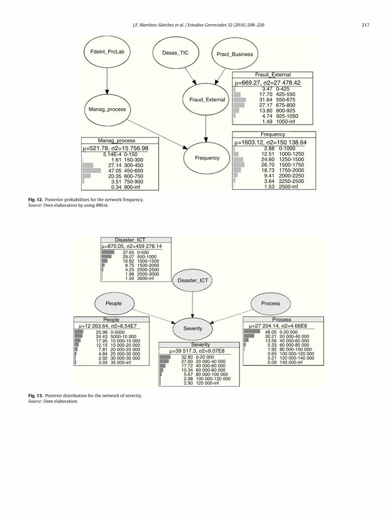
After analyzing each of the networks for frequency and severity,and assigning the corresponding probability distribution func-tions, the posterior probabilities will be now generated. To do this,inference techniques for the Bayesian Networks will be applied.Particularly, we will be using the junction tree algorithm (Guo &Hsu, 2002). The posterior probabilities for nodes of the networkfrequency having at least one parent are shown in Fig. 12.

The results of the node “process management” show that thereis an approximate 2% chance of failures in a segment consid-ering between 150 and 300 events related to the management

J.F. Martínez-Sánchez et al. / Estudios Gerenciales 32 (2016) 208–220 215

9

5.0%

4.5%

5.0%

7.0%

Entrace

Weibull

MinMaxAveStdValues

174.234062.741036.41724.77

80

MinMaxAveStd

169.69+∞

1035.88713.62

245 2229Risk Weibull (1.2199,924.65,RiskShift(169.69))

90.0%

88.4%

8

7

6

5

Va

lue

s in

× 1

0-4

4

3

2

1

0

0

500

1000

1500

2000

2500

3000

3500

4000

4500

Fig. 6. Distribution for disaster and ICT failure.

Source: Own elaboration by using @Risk.

4000

3500

3000

2500

2000

1500

1000

500

Weibull

Risk Weibull (1.2199,924.65,RiskShift(169.69))

0

0

500

1000

1500

2000

2500

3000

3500

4000

4500

Fig. 7. Comparison of quantiles.

Source: Own elaboration by using @Risk.

60 000

50 000

40 000

30 000

20 000

10 000

0

0

10 0

00

20 0

00

30 0

00

40 0

00

50 0

00

60 0

00

Weibull

Risk Weibull (1221,13 372,RiskShift(2441.3))

Fig. 9. Comparison of quantiles.

Source: Own elaboration by using @Risk.

6

5.0%

3533 32 208Risk Weibull (1221,13 372,RiskShift(2441.3))

4.6%

5.0%

7.0%

Input

MinMaxAveStdValues

2517.4458 992.5814 971.5910 476.36

80

Weibull

MinMaxAveStd

2441.30+∞

14 965.0510 309.07

90.0%

88.4%

5

4

3

2

1

0

0

10 0

00

20 0

00

30 0

00

40 0

00

50 0

00

60 0

00

Valu

es in ×

10

-5

Fig. 8. Distribution for losses in human factor.

Source: Own elaboration by using @Risk.

216 J.F. Martínez-Sánchez et al. / Estudios Gerenciales 32 (2016) 208–220

3.0

7477 68 166

5.0%

7.0%

Input

Weibull

MinMaxAveStdValues

5327.97124 853.44

31 683.0222 175.82

80

MinMaxAveStd

5165.60+∞

31 668.4921 828.09

90.0%

88.4%

2.5

2.0

1.5

1.0

0.5

0.0

0

20 0

00

40 0

00

60 0

00

80 0

00

100 0

00

120 0

00

140 0

00

Va

lue

s in

× 1

0-5

Fig. 10. Distribution for losses due to faulty processes.

Source: Own elaboration by using @Risk.

120 000

80 000

60 000

40 000

20 000

0

0

20 0

00

40 0

00

60 0

00

80 0

00

100 0

00

120 0

00

140 0

00

100 000

Weibull

Risk Weibull (1.2203,28 294,RiskShift(5165.6))

Fig. 11. Comparison of quantiles.

Source: Own elaboration by using @Risk.

process over a period of 20 days; a 27% chance of occurrences in asegment considering between 300 and 450 events; a probabilityof 0.47 of having failure occurrences in an interval consideringbetween 450 and 600 events, and a 20% chance in a segmentconsidering between 600 and 750 events associated with theadministration of banking processes. The calculated probabili-ties are conditioned by the presence of events related to internalfraud and work processes.

Regarding the node “external fraud” the occurrences between425 and 550 external frauds over a period of 20 days have anapproximate probability of 0.17; between 550 and 675 eventsa probability of 0.3; between 675 and 800 external fraud theprobability is 0.27; and for more than 800 frauds the probabil-ity is about 0.2. All these probabilities are conditional on theexistence of events related disasters, failures in ICT, and laborpractices.

Finally, the probability distribution of the node “Frequency”shows an approximate 15% chance, over a period of 20 days,that failures occur up to 1250; a probability of 25% in a segmentconsidering between 1250 and 1500; a probability of 0.26 in aninterval considering between 1500 and 1750 failures; an approx-imate 19% chance in a segment considering between 1750 and2000 events; a probability of 0.9 in a segment containing between2000 and 2250 failures, and approximately 5% chance that 2250failures occur over a period of 20 days. These are the conditional

probabilities to risk factors such as external fraud, process effi-ciency and people reliability.

Finally, it is important to point out that for determining theprobabilities of each node in the frequency network, the negativebinomial plays an important role since there is significant empir-ical evidence that the frequency of operational risk events havean adequate fit under this distribution. In the case of the networkof severity, it has the posterior distribution shown in Fig. 13.

The losses caused by human errors on average are 12,263 Eurosin periods of 20 days. With regard to losses for catastrophic eventssuch as demonstrations, floods, and ICT failure, among others, areon average 870 Euros. In terms of process failures on average theyhave a loss every 20 days of 27,204 Euros. The probability distri-bution of the node “Severity” shows that there is a probabilityof 0.33 of the occurrence of a loss between 0 and 20,000 Euros;a probability of 0.2 between 20,000 and 40,000, a 10% chancebetween 60,000 and 80,000 Euros, a 6% chance between 80,000and 100,000 Euros, and approximately a 6% chance that the lossbe greater than 100,000 Euros in a period of 20 days.

6. Value at operational risk

Once we have carried out the Bayesian inference process toobtain posterior distributions for the frequency of OR events and theseverity of losses in the previous section, we now proceed to inte-grate both distributions through Monte Carlo8 simulation by usingthe “Compound” function of @Risk. To achieve this goal, we gener-ate the distribution function of potential losses by using a negativebinomial for frequency and an extreme value Weibull distributionfor severity.9 It is worthy to mention that Monte Carlo simula-tion method has the disadvantage that it requires high processingcapacity and, of course, is based on a random number genera-tor. For the calculation of OpVar the values obtained are arrangedfor expected losses in descending order and the correspondingpercentiles are calculated in Table 3. Accordingly, if we calculatethe OpVaR with a confidence level of 95%, we have a maximumexpected loss of D 88.4 million over a period of 20 days for the groupof international banks associated to the ORX.10

8 The simulation results are available via e-mail request marzan67@gmail.com.9 Other alternative statistical method is the copula approach, though not always

a closed solution can be found.10 For a complete list of banks associated see http://www.orx.org/orx-members.

J.F. Martínez-Sánchez et al. / Estudios Gerenciales 32 (2016) 208–220 217

Fdelnt_PrcLab Desas_TIC Pract_Business

Fraud_External

Frequency

Fraud_External

Manag_process

Manag_process

5.14E-41.61

27.1447.0520.353.510.34

0-150150-300300-450450-600600-750750-900900-inf

µ=521.78, σ2=15 756.98 2.8812.5124.6026.7018.739.413.641.53

0-425425-550550-675675-800800-925925-10501050-inf

3.4717.7031.6427.1713.804.741.49

µ=669.27, σ2=27 478.42

Frequency

0-10001000-12501250-15001500-17501750-20002000-22502250-25002500-inf

µ=1603.12, σ2=150 138.64

Fig. 12. Posterior probabilities for the network frequency.

Source: Own elaboration by using @Risk.

Disaster_ICT

Disaster_ICT

37.6529.0716.828.754.251.961.50

0-500500-10001000-15001500-20002000-25002500-30003000-inf

µ=870.05, σ2=459 278.14

People

People

25.9824.4317.9512.157.814.842.923.93

0-50005000-10 00010 000-15 00015 000-20 00020 000-25 00025 000-30 00030 000-35 00035 000-inf

µ=12 263.64, σ2=8.54E7

Severity

Severity

32.8027.6017.7210.34

5.672.982.90

0-20 00020 000-40 00040 000-60 00060 000-80 00080 000-100 000100 000-120 000120 000-inf

µ=39 517.3, σ2=9.07E8

Process

Process

48.0530.2113.56

5.331.920.650.210.09

0-20 00020 000-40 00040 000-60 00060 000-80 00080 000-100 000100 000-120 000120 000-140 000140 000-inf

µ=27 204.14, σ2=4.66E8

Fig. 13. Posterior distribution for the network of severity.

Source: Own elaboration.

218 J.F. Martínez-Sánchez et al. / Estudios Gerenciales 32 (2016) 208–220

Table 3

Percentiles for Bayesian model.

Position Losses (D ) Percentage

9622 135,413,727.38 100.00%

8982 131,176,038.11 99.90%

9435 130,218,813.55 99.90%

6995 129,793,806.36 99.90%

6645 124,593,969.74 99.90%

6487 124,470,160.96 99.90%

1516 122,407,799.73 99.90%

8881 118,657,656.06 99.90%

771 117,984,437.39 99.90%

7645 117,606,673.03 99.90%

2305 116,262,949.32 99.80%

5024 115,407,667.31 99.80%

6449 115,283,482.79 99.80%

999 114,692,910.29 99.80%

2060 114,195,679.10 99.80%

3720 113,461,486.17 99.80%

4120 113,391,200.37 99.80%

5088 113,293,233.82 99.80%

1789 113,079,925.31 99.80%

64 112,978,179.49 99.80%

. . .

2559 96,082,951.45 98.10%

2607 96,036,899.87 98.00%

8393 96,036,097.99 98.00%

3877 95,957,705.18 98.00%

5895 95,901,765.22 98.00%

8329 95,865,557.01 98.00%

1213 95,858,547.94 98.00%

7940 95,847,089.05 98.00%

5866 95,696,438.40 98.00%

4608 95,696,191.31 98.00%

7151 95,632,162.12 98.00%

5939 95,455,846.07 97.90%

6161 95,409,510.44 97.90%

622 95,367,523.21 97.90%

6899 95,311,650.62 97.90%

3771 95,304,390.04 97.90%

3042 95,265,269.48 97.90%

1256 95,261,114.91 97.90%

9712 95,256,473.11 97.90%

1943 95,139,840.10 97.90%

1038 95,132,874.12 97.90%

. . .

9618 88,408,111.80 95.10%

2989 88,406,427.34 95.10%

8131 88,400,173.73 95.00%

8446 88,396,425.98 95.00%

7811 88,293,244.91 95.00%

940 88,288,312.72 95.00%

7655 88,285,525.53 95.00%

4666 88,207,565.35 95.00%

4654 88,165,650.42 95.00%

9973 88,152,913.81 95.00%

6944 88,149,275.18 95.00%

9940 88,146,575.13 95.00%

7528 88,110,981.98 94.90%

2222 88,095,871.13 94.90%

2657 88,075,028.67 94.90%

3163 88,064,696.68 94.90%

9360 88,057,973.00 94.90%

7694 88,053,418.86 94.90%

9256 88,048,859.73 94.90%

7542 88,044,642.79 94.90%

3059 88,025,745.60 94.90%

Source: Own elaboration.

7. Conclusions

Transnational banks generate large amounts of informationfrom the interaction with customers, with the industry and withinternal processes. However, the interaction with the individualsinvolved in the processes and systems also required some attention

and this considered by the Operational Riskdata eXchange Asso-ciation that has stated several standards for the registration andmeasurement of operational risk.

This paper has provided the theoretical elements and practi-cal guidance necessary to identify, quantify and manage OR in theinternational banking sector under the Bayesian approach. Thisresearch uses elements more attached to reality such as: spe-cific probability distributions (discrete or continuous) for each riskfactor, additional data and information updating the model, andrelationships (causality) of risk factors. It was shown that the BNframework is a viable option for managing OR in an environmentof uncertainty and scarce information or with questionable quality.The capital requirement is calculated by combining statistical datawith opinions and judgments of experts, as well as, external infor-mation, which is more consistent with reality. The BNs as a toolfor managing OR in lines of business of the international bankingsector have several advantages over other models:

• The BN is able to incorporate the four essential elements ofAdvanced Measurement Approach (AMA): internal data, exter-nal data, scenario analysis and factors reflecting the businessenvironment and the control system in a simple model.

• The BN can be built into a “multi-level” model, which can displayvarious levels of dependency between the various risk factors.

• The BN running on a network of decision can provide a cost-benefit analysis of risk factors, where the optimum controls aredetermined within a scenario analysis.

• The BN is a direct representation of the real world, not a way ofthinking as neural networks. Arrows or arcs in networks standfor the actual causal connections.

It is important to point out that the CVaR used in the Bayesianapproach is consistent in the sense of Artzner et al. (1999), butalso summarizes the complex causal relationships between the dif-ferent risk factors that result in operational risk events. In short,because the reality is much more complex than independent eventsidentically distributed, the Bayesian approach is an alternative tomodel a complex and dynamic reality.

Finally, among the main empirical results, it is worth mention-ing that after calculating the OpVaR, with a confidence level of 95%,the maximum expected loss over a period of 20 days for the groupof international banks associated to the ORX was D 88.4 million,which is a significant amount to be considered to manage opera-tional risk in ORX for the studied lines of business of commercialbanks.

Conflict of interests

The authors declare no conflict of interest.

Appendix. An exact algorithm for Bayesian inference

Among the accurate inference algorithms, we have: Pearl’s(1988) polytree; Lauritzen and Spiegelhalter (1988) clique tree, andCowell, Dawid, Lauritzen, and Spiegelhalter’s (1999) junction tree.Pearl’s method is one of the earliest and most widely used. Thespread of beliefs according to Pearl (1988) follow the following pro-cess. Let e be the set of values for all observed variables. For anyvariable X, e can be divided into two subsets: e−

X representing allthe observed variables descending from X, and e+

X correspondingto all other observed variables. The impact of the observed vari-ables on the beliefs of X can be represented by the following twovalues:

�(X) = P(e−

X |X) (A1)

J.F. Martínez-Sánchez et al. / Estudios Gerenciales 32 (2016) 208–220 219

�(X) = P(e+

X |X). (A2)

That is, �(X) and �(X) are vectors whose elements are associatedwith the values of X:

�(X) = [�(X = x1), �(X = x2), . . ., �(X = xl)] (A3)

�(X) = [�(X = x1), �(X = x2), . . ., �(X = xl)] (A4)

The posterior distribution is obtained by using (A1) and (A2),thus

P(X|e) = ˛�(X)�(X) (A5)

where = 1/P(e). In order to infer new beliefs, Eq. (A5) is used. Thevalues of �(X) and �(X) are calculated as follows: �(Y1, Y2, . . ., Ym)where Y1, Y2, . . ., Ym are children of X. When X takes the value x0,the elements of vector �(X) are assigned as follows:

�(xi) =

{

0 si xi /= x0.1 si xi = x0.

In the case in which X has no value, we have e−

X =⋃m

i=1e−

yi. Hence,

by using (A1), �(X) expands as:

�(X) = P(e−

X |X) (A6)

= P(e−y1

, e−y2

, . . ., e−ym

|X) (A7)

= P(e−y1

|X)P(e−y2

|X)· · ·P(e−ym

|X) (A8)

= �y1(X)�y2

(X). . .�ym (X), (A9)

By using the fact that e−y1

, e−y2

, . . ., e−ym

are conditionally inde-pendent, and defining

�yi(X) = P(e−

X |X),

it follows that

�yi(X) = P(e−

Y |X) (A10)

=

∑

yi

P(e−yi

, yi|X) (A11)

=

∑

yi

P(e−yi

|yi, X)P(yi|X) (A12)

=

∑

yi

P(e−yi

|yi)P(yi|X) (A13)

=

∑

yi

�yiP(yi|X). (A14)

The last expression shows that in calculating the value of �(X)the values of � and conditional probabilities of all children X arerequired. Therefore, vector �(X) is calculated as:

�(X) = ˘c ∈ children (X)

∑

v ∈ c

�(v)P(v|X). (A15)

For the calculation of �(X) it is used the father Y of the X values.Indeed, by using (A2), it follows

�(X) = P(X|e+

X ) (A16)

=

∑

yi

P(X, yi|e+

Xi) (A17)

=

∑

yi

P(X|yi, e+

Xi)P(yi|e

+

X ) (A18)

=

∑

yi

P(X|yi)P(yi|e+

X ) (A19)

=

∑

yi

P(X|yi, e+

Xi) �(yi). (A20)

This shows that when calculating �(X), the values of � of thefathers X and their conditional probabilities are necessary.

There might be some difficulties in dealing with Pearl’s infer-ence method due to the generated cycles when the directionalityis eliminated. Cowell et al. (1999) junction tree algorithm mayovercome this situation. First, it converts a directed graph intoa tree whose nodes are closed to proceed to spread the valuesof � and � through the tree. The summarized procedure is asfollows:

1. “Moralize” the BN.2. Triangulate the moralized graph.3. Let the cliques of the triangulated graph be the nodes of a tree,

which is the desired junction-tree.4. Propagate � and � values throughout the junction-tree to make

inference. Propagation will produce posterior probabilities.

References

Aquaro, V., Bardoscia, M., Belloti, R., Consiglio, A., De Carlo, F., & Ferri, G. (2009). ABayesian networks approach to operational risk. Physica A: Statistical Mechanicsand its Applications, 389(8), 1721–1728.

Alexander, C. (2002). Operational risk measurement: Advanced approaches. UK:ISMA Centre. University of Reading. Retrieved from: http://www.dofin.ase.ro/Lectures/Alexander%20Carol/Oprisk Bucharest.pdf

Artzner, P., Delbaen, F., Eber, J., & Heath, D. (1999). Coherent measures of risk. Math-ematical Finance, 9(3), 203–228.

Basel II. (2001a). Operational risk. Consultative document. Retrieved from:https://www.bis.org/publ/bcbsca07.pdf

Basel II. (2001b). Working paper on the regulatory treatment of operational risk.Retrieved from: http://www.bis.org/publ/bcbs wp8.pdf

Carrillo-Menéndez, S., & Suárez-González, A. (2015). Challenges in operational riskmodelling. In International Model Risk Management Conference. Retrieved from:http://imrmcon.org/wp-content/uploads/2015/06/CS-5B Model-Risk-Within-Operational-Risk1.pdf

Carrillo-Menéndez, S., Marhuenda-Menéndez, M., & Suárez-González, A.(2007). El entorno AMA (Advanced Model Approach). Los datos ysu tratamiento. In Ana Fernández-Laviada (Ed.), La gestión del riesgooperacional: de la teoría a su aplicación. Santander: Universidad deCantabria.

Cowell, R., Dawid, G., Lauritzen, A. P., & Spiegelhalter, D. J. (1999). Probabilisticnetworks and expert systems. Berlin: Springer-Verlag.

Cruz, M. G. (2002). Modeling, measuring and hedging operational risk. In Series WileyFinance. West Sussex, UK: John Wiley & Sons.

Cruz, M. G., Peters, G. W., & Shevchenko, P. V. (2002). Fundamental aspects of opera-tional risk and insurance analytics: A handbook of operational risk. New York: JohnWiley & Sons.

Degen, M., Embrechts, P., & Lambrigger, D. (2007). The quantitative model-ing of operational risk: Between g-and-h and EVT. Switzerland: Depart-ment of Mathematics, ETH Zurich, CH-8092 Zurich. Retrieved from:https://people.math.ethz.ch/∼embrecht/ftp/g-and-h May07.pdf

Embrechts, P., Furrer, H., & Kaufmann, O. (2003). Quantifying regulatory cap-ital for operational risk. Derivatives Use, Trading and Regulation, 9(3),217–233.

Ferguson, T. S. (1973). A Bayesian analysis of some nonparametric problems. Annalsof Statistics, 2(4), 615–629.

Guo, H., & Hsu, W. (2002). A survey of algorithms for real-time Bayesian net-work inference. In Join Workshop on Real Time Decision Support and DiagnosisSystems.

Heinrich, G. (2006). Riesgo operacional, pagos, sistemas de pago y aplicación de BasileaII en América Latina: evolución más reciente. Boletín del CEMLA. Retrieved from:https://www.bis.org/repofficepubl/heinrich riesgo operacional a.pdf

Jensen, F. V. (1996). An introduction to Bayesian networks (1st ed.). London: UCL Press.Kartik, A., & Reimer, K. (2007). Phase transitions in operational risk. Physical Review

E, 75(1 part 2), 1–14.Lauritzen, S. L., & Spiegelhalter, D. J. (1988). Local computations with probabilities

on graphical structures and their application to expert systems. Journal of RoyalStatistical Society, Series B, 50(2), 157–224.

Moscadelli, M. (2004). The modelling of operational risk: Experience with theanalysis of the data collected by the Basel committee. Bank of Italy, WorkingPaper, N◦157. Retrieved from: https://www.bancaditalia.it/pubblicazioni/temi-discussione/2004/2004-0517/tema 517.pdf?language id=1

Neil, M., Marquez, D., & Fenton, N. (2004). Bayesian networks to model expected andunexpected operational losses. Risk Analysis, 25(4), 675–689.

Panjer, H. (2006). Operational risk. Modeling analytics (1st ed.). Hoboken, NJ: Wiley-Interscience.

Pearl, J. (1988). Probabilistic Reasoning in Intelligent Systems: Networks of PlausibleInference (first edition). San Francisco, CA, USA: Morgan Kaufmann Series inRepresentation and Reasoning.

Pearl, J. (2000). Causality, models, reasoning, and inference. London: Cambridge Uni-versity Press.

220 J.F. Martínez-Sánchez et al. / Estudios Gerenciales 32 (2016) 208–220

Reimer, K., & Neu, P. (2003). Functional correlation approach to operational riskin banking organizations. Physica A: Statistical Mechanics and its Applications,322(1), 650–666.

Reimer, K., & Neu, P. (2002). Adequate capital and stress testing for operational risks.Physical Review E, 75(1), 016111.

Supatgiat, C., Kenyon, C., & Heusler, L. (2006). Cause-to-effect operational risk quan-tification and management. Risk Management, 8(1), 16–42.

Venegas-Martínez, F. (2006). Riesgos financieros y económicos. Productos derivadosy decisiones económicas bajo incertidumbre (1a. Ed.). México D.F.: InternationalThomson Editors.

Zellner, A. (1971). An Introduction to Bayesian inference in econometrics. New York:Wiley.