operational risk management { implementing a bayesian
TRANSCRIPT

Operational Risk management –
Implementing a Bayesian Network for
Foreign Exchange and Money Market
Settlement
Dissertation
Presented for the Degree of Doctor of Philosophy at the Faculty of Economics
and Business Administration of
the University of Gottingen
by
Kwabena Adusei-Pokufrom Kumasi, Ghana.
Gottingen, 2005

First Examiner: Prof. Dr. Walter Zucchini
Second Examiner: Prof. Dr. Wolfgang Benner
Date of oral exams: 26.08.2005

To Edith,
for all the sacrifices you made.


Acknowledgements
This work was completed during my stay at the Institute of Statistics and Econo-
metrics of the Faculty of Economics and Business Administration, University of
Goettingen while participating in the Ph.D program of the Center of Statistics.
Like all major endeavours, one receives help, guidance and encouragement, which
must be acknowledged.
I wish to thank my advisor Prof. Dr. Walter Zucchini for the guidance and en-
couragement he gave me throughout my stay at the Institute. I particularly ap-
preciate his patience and willingness to help at all times without which this work
would not have been completed. Many thanks to Marcelo G. Cruz of RiskMaths
Consulting and Jack L. King of Genoa (UK) Limited for the comments and sug-
gestions they provided during the initial stages of the work. Gerrit van den Brink
and Helmut Heiming of Dresdner Bank deserve special thanks for helping with
the supervision of the work and providing the needed practical insights as well as
helping me appreciate operational risk the more. Particular thanks are also due
to Patricia Licht and Edgar Peters.
Special thanks to Oleg Nenadic of the Institute of Statistics and Econometrics
for the numerous help he provided in statistical programing and LaTex. Thanks
to Prof. Dr. Wolfgang Benner and PD. Dr. Andreas Nickel for accepting to be
my second and third examiners respectively. I also wish to thank Prof. Manfred
Denker of the Center for Statistics for arranging the funding for this work.
Finally and most importantly, my most sincerest thanks to my wife, Edith, for her
love, support and understanding, which I have greatly benefited from. Thank you
Edith for proof reading the script and especially, caring for our children (Serwa
and Kwame) during this major endeavour.


Contents
1 Introduction and Motivation 1
1.1 Introduction . . . . . . . . . . . . . . . . . . . . . . . . . . . . . . 1
1.2 Motivation and Problem Description . . . . . . . . . . . . . . . . 2
1.3 Objectives of Research . . . . . . . . . . . . . . . . . . . . . . . . 3
1.4 Outline of the Thesis . . . . . . . . . . . . . . . . . . . . . . . . . 3
2 Operational Risk, Foreign Exchange and Money Market 5
2.1 Basel II, Operational Risk and Sarbanes-Oxley . . . . . . . . . . . 5
2.2 The Foreign Exchange and Money Markets . . . . . . . . . . . . . 8
2.3 Operational Risk in Foreign Exchange and Money Market . . . . 10
2.4 Review of Operational Risk Methods . . . . . . . . . . . . . . . . 13
2.4.1 Models for Quantification and Capital Allocation . . . . . 13
2.4.1.1 Loss Distribution Approach . . . . . . . . . . . . 14
2.4.1.2 The Scorecard or Risk Drivers and Controls Ap-
proach . . . . . . . . . . . . . . . . . . . . . . . . 17
2.4.1.3 Scenario-Based Approach . . . . . . . . . . . . . 18
2.4.2 Models for Managing OR . . . . . . . . . . . . . . . . . . . 19
2.5 Assessment of Bayesian Networks for Operational Risk Management 22
2.5.1 Prospects of Bayesian Networks for Operational Risk . . . 22
2.5.2 Criticisms of Bayesian Networks in Operational Risks Ap-
plication . . . . . . . . . . . . . . . . . . . . . . . . . . . . 23
3 Bayesian Networks 25

ii CONTENTS
3.1 Introduction on Bayesian Networks . . . . . . . . . . . . . . . . . 25
3.2 Areas of Application . . . . . . . . . . . . . . . . . . . . . . . . . 27
3.3 Theory of Bayesian Networks . . . . . . . . . . . . . . . . . . . . 27
3.3.1 The Chain Rule for Bayesian Networks . . . . . . . . . . . 28
3.3.2 Algorithms for Evaluating Bayesian Networks . . . . . . . 28
3.3.2.1 Exact Inference Algorithms . . . . . . . . . . . . 29
3.3.2.2 Approximate Inference Algorithms . . . . . . . . 32
3.4 Realization of Bayesian Network . . . . . . . . . . . . . . . . . . 33
3.4.1 Nodes, Network and Structural Validation . . . . . . . . . 34
3.5 Quantifying the Network . . . . . . . . . . . . . . . . . . . . . . . 36
3.5.1 Probability Elicitation . . . . . . . . . . . . . . . . . . . . 36
3.5.2 Protocols and Bias . . . . . . . . . . . . . . . . . . . . . . 37
3.5.3 Validation of Estimates . . . . . . . . . . . . . . . . . . . . 39
3.6 Strengths and Limitations of Bayesian Networks . . . . . . . . . . 40
3.6.1 Concluding Remarks . . . . . . . . . . . . . . . . . . . . . 41
4 Introduction to the Case Study 43
4.1 Introduction . . . . . . . . . . . . . . . . . . . . . . . . . . . . . . 43
4.2 Problem Description . . . . . . . . . . . . . . . . . . . . . . . . . 43
4.3 Specific Objectives in this Case Study . . . . . . . . . . . . . . . . 44
4.4 Scope of Modeling and Decisions . . . . . . . . . . . . . . . . . . 44
5 Construction of a Bayesian Network for Foreign Exchange Set-
tlement 47
5.1 The Foreign Exchange and Money Market Settlement Process . . 47
5.2 Building the Network . . . . . . . . . . . . . . . . . . . . . . . . . 48
5.3 Structural Model Building . . . . . . . . . . . . . . . . . . . . . . 49
5.3.1 Risk, Process Mapping and Nodes Identification . . . . . . 49
5.3.2 Network Structure . . . . . . . . . . . . . . . . . . . . . . 51
5.3.3 Conditional Probability and Node Description Tables . . . 54

CONTENTS iii
5.3.4 Model Structure Validation . . . . . . . . . . . . . . . . . 57
5.4 Quantifying the Network . . . . . . . . . . . . . . . . . . . . . . . 58
5.4.1 Objective Data . . . . . . . . . . . . . . . . . . . . . . . . 58
5.4.2 The Elicitation Process . . . . . . . . . . . . . . . . . . . . 59
5.4.3 Protocol, Instruments and Procedures . . . . . . . . . . . 60
5.4.4 Conducting the Elicitation . . . . . . . . . . . . . . . . . . 64
5.4.5 Validating the Estimates . . . . . . . . . . . . . . . . . . . 67
5.5 Data Processing . . . . . . . . . . . . . . . . . . . . . . . . . . . . 69
5.5.1 Frequency Data . . . . . . . . . . . . . . . . . . . . . . . . 69
5.5.2 Loss Severity Data . . . . . . . . . . . . . . . . . . . . . . 70
5.5.3 Loss Severity - Probability Computations . . . . . . . . . . 75
5.6 Aggregating the Frequency and Severity Outputs through Monte-
Carlo Simulation . . . . . . . . . . . . . . . . . . . . . . . . . . . 78
5.7 Maintaining the network . . . . . . . . . . . . . . . . . . . . . . . 80
6 Results, Validation and Applications 81
6.1 Model Results . . . . . . . . . . . . . . . . . . . . . . . . . . . . . 81
6.1.1 Results – Frequency of Failure and Severity of Losses . . . 81
6.1.2 Results – Aggregated Potential Losses . . . . . . . . . . . 83
6.1.3 Results – Operational Value at Risk . . . . . . . . . . . . . 84
6.2 Model Validation . . . . . . . . . . . . . . . . . . . . . . . . . . . 85
6.2.1 Comparison of Results – Frequency of Failures . . . . . . . 86
6.2.2 Comparison of Results – Severity of Losses . . . . . . . . . 87
6.2.3 Comparison of Results – Potential Losses . . . . . . . . . . 89
6.3 Managing Operational Risk with the Model . . . . . . . . . . . . 94
6.3.1 Managing the Drivers of Loss Severity . . . . . . . . . . . 95
6.3.2 Managing the Drivers of Frequency of Failures . . . . . . . 101
6.3.3 Prediction of Operational Value at Risk . . . . . . . . . . 107
7 Summary and Conclusions 109

iv CONTENTS
7.1 Summary of Work . . . . . . . . . . . . . . . . . . . . . . . . . . 109
7.2 Further Work . . . . . . . . . . . . . . . . . . . . . . . . . . . . . 111
7.3 Conclusion . . . . . . . . . . . . . . . . . . . . . . . . . . . . . . . 112
A Questionnaire 113
B Prior Probabilities 123

List of Figures
2.1 Economic capital, unexpected and expected loss . . . . . . . . . . 16
3.1 An example of a Bayesian network . . . . . . . . . . . . . . . . . 26
3.2 A BN flow diagram . . . . . . . . . . . . . . . . . . . . . . . . . . 34
5.1 FX process flow. Source: The Foreign Exchange Committee, Fed-
eral Reserve Bank of New York . . . . . . . . . . . . . . . . . . . 48
5.2 Frequency of failure network . . . . . . . . . . . . . . . . . . . . . 53
5.3 Loss severity network . . . . . . . . . . . . . . . . . . . . . . . . . 54
5.4 Typical questionnaire format . . . . . . . . . . . . . . . . . . . . . 63
5.5 Exploratory graphs of some trade values . . . . . . . . . . . . . . 72
5.6 Kernel density estimation . . . . . . . . . . . . . . . . . . . . . . 74
5.7 Assessing goodness of fit . . . . . . . . . . . . . . . . . . . . . . . 75
5.8 Aggregating frequency and severity distributions . . . . . . . . . . 78
6.1 Frequency network showing some posterior probabilities . . . . . . 82
6.2 Severity network showing some posterior probabilities . . . . . . . 83
6.3 Histogram of potential losses . . . . . . . . . . . . . . . . . . . . . 84
6.4 Comparison of frequency of failure . . . . . . . . . . . . . . . . . . 87
6.5 Commulative distribution function of losses (logscale) . . . . . . . 88
6.6 QQ plots of losses with truncations at 100, 500 and 1000 EUR . . 89
6.7 Potential loss - cdf comparison . . . . . . . . . . . . . . . . . . . . 91
6.8 Potential loss - qq plots I (model versus historical data) . . . . . . 92
6.9 Potential loss - qq plots II (model versus historical data) . . . . . 93

2 LIST OF FIGURES
6.10 Illustration SI - largest loss amount . . . . . . . . . . . . . . . . . 96
6.11 Illustration SI - loss with days delay . . . . . . . . . . . . . . . . . 97
6.12 Illustration SII - stop loss with most likely combination of states . 98
6.13 Probability curves for various days delays (daysdelay = 1 is solid
line, 2 is dash, 3 is longdash, 4 is dotdash and 5 is dotted). Vertical
line is the 50m EUR trade value . . . . . . . . . . . . . . . . . . . 100
6.14 Illustration SIII - days delay scenario . . . . . . . . . . . . . . . . 101
6.15 Illustration FI - back office system failure . . . . . . . . . . . . . . 102
6.16 Illustration FI - effect of trade volume on systems . . . . . . . . . 103
6.17 Illustration FII - causes of vulnerability to failure . . . . . . . . . 104
6.18 Illustration FII - effect of quality of SSI . . . . . . . . . . . . . . . 105
6.19 Illustration FIII - most sensitive nodes . . . . . . . . . . . . . . . 105
6.20 Illustration FIII - most sensitive nodes . . . . . . . . . . . . . . . 107
A.1 Questionnaire introduction . . . . . . . . . . . . . . . . . . . . . . 114
A.2 Questionaire introduction - bias . . . . . . . . . . . . . . . . . . . 115
A.3 Questionnaire introduction - interview information . . . . . . . . . 115
A.4 Sample Questionaire - trade volume . . . . . . . . . . . . . . . . . 116
A.5 Sample Questionnaire - gross or netting settlement . . . . . . . . 117
A.6 Sample Questionnaire - days delay (1) . . . . . . . . . . . . . . . 118
A.7 Sample Questionnaire - days delay (2) . . . . . . . . . . . . . . . 119

List of Tables
5.1 Risk and process mapping . . . . . . . . . . . . . . . . . . . . . . 50
5.2 Node description table - frequency of failures . . . . . . . . . . . . 56
5.3 Node Description Table - severity of losses . . . . . . . . . . . . . 57
5.4 Currency distribution and interest rates . . . . . . . . . . . . . . . 71
5.5 Monte-Carlo simulations . . . . . . . . . . . . . . . . . . . . . . . 79
6.1 Summary statistics of potential loss . . . . . . . . . . . . . . . . . 83
6.2 Operational risk unexpected loss . . . . . . . . . . . . . . . . . . . 85
6.3 Operational risk unexpected loss . . . . . . . . . . . . . . . . . . . 90
A.1 Matrix format questionnaire - Confirmation matching . . . . . . . 120
A.2 Matrix format questionnaire - Number of settlement failure . . . . 121
B.1 Elicited probabilities - frequency of failure I . . . . . . . . . . . . 124
B.2 Elicited probabilities - frequency of failure II . . . . . . . . . . . . 125
B.3 Elicited probabilities - loss severity network . . . . . . . . . . . . 126
B.4 Days delay node probabilities - with logit adjustments for illustra-
tion SIII in chapter 6 . . . . . . . . . . . . . . . . . . . . . . . . . 126


List of Abbreviations
ACI International Financial Markets Association
AIB Allied Irish Bank
AMA Advanced Measurement Approach
BIS Bank for International Settlement
BN Bayesian Network
CFP Committee for Professionalism – ACI
CLS Continuously Linked Settlement
CPT Conditional Probability Tables
CSA Control Self Assessment
DAG Directed Acyclic Graph
FX Foreign Exchange
KRI Key Risk Indicator
LDA Loss Distribution Approach
MCMC Markov Chain Monte - Carlo Simulation
MM Money Market
NAB National Australian Bank
NDT Node Description Table
OpVaR Operational Value at Risk
OR Operational Risk
OTC Over The Counter
SI Settlement Instructions
SOX Sarbanes Oxley Act
STP Straight Through Process
VaR Value at Risk

Currencies
AUD Australian dollar
BRL Brazilian real
CAD Canadian dollar
CHF Swiss franc
CZK Czech koruna
DKK Danish krone
EUR Euro
GBP Great Britain Pound Sterling
HKD Hong Kong dollar
HUF Hungarian forint
JPY Japanese yen
MXN Mexican peso
NOK Norwegian krone
NZD New Zealand dollar
PLN Polish zloty
RUB Russian ruble
SEK Swedish krona
SGD Singapore dollar
SKK Slovak koruna
TRL Turkish Lira
USD American dollar
ZAR South African rand

Chapter 1
Introduction and Motivation
1.1 Introduction
Recent financial scandals in the banking industry have caused considerable at-
tention to be focused on operational risk. This is because an analysis of some of
these scandals reveals that the underlying causes of these huge financial losses are
due to Operational Risk (OR) and not to credit or market risk, as might initially
appeared to be the case.
The Foreign Exchange (FX) market has had its fair share of these recent scandals.
Two most recent examples of operational risk losses in the FX markets are the
National Australia Bank’s 227 million USD loss in 2004 and Allied Irish Bank’s
750 million USD loss in 2002. These losses have had serious negative impact
on the firms’ profitability and reputation. Besides scandalous losses in the FX
market, trade processing and settlement errors, as well as incorrect settlement,
if not controlled, may lead to indirect costs such as compensation payments to
counterparties, or to the development of large losses in a firm’s portfolio due to
managing the wrong position. Operational risk losses in the financial industry
usually occur at the business unit level and are due to weak management over-
sight, weak internal controls or the lack of it, or to breakdown of proceedures
among others. Operational risk therefore has to be managed at the business unit
level.
This thesis is about managing OR at the business unit (micro) level. It concen-
trates on FX and Money Market (MM) settlement processes and uses Bayesian
belief networks (BN) as a tool to model the causal relationships between risk fac-
tors and Key Risk Indicators (KRI) within the FX and MM settlement process.

2 CHAPTER 1. INTRODUCTION AND MOTIVATION
Such a causal model is able to help risk managers understand the drivers of losses,
to make predictions and also to assess the effects of possible interventions.
1.2 Motivation and Problem Description
The development of operational risk models has evolved rapidly over recent years.
There are basically two reasons to this. One is external; banking regulatory
compliance (Basel II Accord is coming into effect in late 2006) and the other is
internal; most banks are realising that good operational risk management is a
sound business practice. The influence of regulatory compliance is currently the
greater of the two. Consequently, managing OR as done in banks is presently at
the ”macro”, or top level and banks are more concerned, as it were, with getting
their operational risk capital models approved by banking regulators. This trend
is expected to continue for some time.
It is envisaged that after banks have achieved their first target of capital compu-
tation, their attention will be turned to managing operational risk at the ”micro”
or business unit level. It is at the micro level that operational risk losses actually
occur. This makes managing OR at the business unit level the next logical stage
of OR development. With this shift, emphasis will consequently be placed on
models used for managing OR at the business unit level. Presently, models for
managing operational risk at the business unit level are the Key Risk Indica-
tors and causal models (for example, multifactor models and Bayesian networks)
among others. Key Risk Indicators are the most widely used whereas the causal
models are not well studied and documented.
A Bayesian belief network, is a tool which can relate and show the causal relation-
ship among risk factors, key risk indicators and some operational risk attributes.
Such a causal model is very useful in managing OR at the business unit level
since it can perform predictions under various scenarios, that is, perform ”what-
if-analysis” and show the results of possible interventions immediately. Alexander
(2003), King (2001) and Ramamurthy et al. (2005) have made some attempts at
demonstrating the usefulness of BN in managing OR at the business unit level.
Other researchers like Giudici (2004) and Neil et al. (2005) however, emphasize
BN as a tool for computing economic capital.
Significantly missing in the available literature on OR is a complete practical guid-
ance on how a BN can be implemented in a real-world situation from the point
of realising the network structure, through probability elicitations and managing
OR with the model to maintain the BN. The absence of this detailed procedural

CHAPTER 1. INTRODUCTION AND MOTIVATION 3
guide has lead to OR practioners, who might agree on the usefulness of BN, to
conclude that BNs are too complex to construct and maintain, and that gives
insufficient return for the effort. This is what has contributed to the under uti-
lization of Bayesian network technology in operational risk management although
BNs have had great successes in other fields of study. This thesis addresses these
issues and, in particular, provides an illustration of how one can go about applying
Bayesian networks in a practical setting.
1.3 Objectives of Research
The objectives of this thesis are
1. to provide a complete practical procedural guidance on how a BN can be
implemented as a causal model for the purpose of managing operational
risk in a specific business line or business unit.
2. to re-affirm the usefulness of a BN and also to demonstrate how a BN can
be used to manage OR in a real - world situation.
These objectives are achieved through 1) the construction of a BN for FX and
MM settlement process in a bank. The BN establishes the causal relationship
between the necessary risk factors, key risk indicators and other operational risk
attributes; and 2) the application of the network to FX and MM process to assist
in understanding the drivers of operational risk and the effects of possible inter-
ventions, and to compute an economic capital for OR for internal management
purposes.
1.4 Outline of the Thesis
This thesis is divided into two parts; Part I and Part II. Part I is captioned
”Background, Literature and Available Approaches” and includes Chapters 1, 2,
and 3. Chapter 1 introduces and motivates the thesis, and sets out the objectives
of the thesis. Chapter 2 provides the background to operational risk, foreign ex-
change and money markets, and reveiws the available approaches to quantifiying
and managing operational risk. It ends with the assertion that Bayesian net-
works provide a powerful tool for managing operational risk. The theory behind
Bayesian networks, and how they are realized (including the elicitation of expert
opinion) is presented in Chapter 3.

4 CHAPTER 1. INTRODUCTION AND MOTIVATION
Part II is a case study titled ”Application of BN to FX and MM settlement”. It
shows a practical application of BN to FX and MM settlement. It starts with
defining and establishing the objectives of the BN in Chapter 4 and proceeds to
how the BN model is constructed and quantified in Chapter 5. Chapter 6 shows
the results of applying BN model to FX settlement and also illustrates how the
model can be used to manage operational risk. The summary and conclusions of
the thesis is given in Chapter 7.

Chapter 2
Operational Risk, Foreign
Exchange and Money Market
2.1 Basel II, Operational Risk and Sarbanes-
Oxley
The Basel Committee on Banking Supervision (The Committee) of the Bank of
International Settlement has been working for several years on the New Basel
Accord, known as Basel II to replace the old Accord, known as Basel I, which
was published in 1988. In June 2004, the Committee published the much awaited
”Basel II” framework for bank capital adequacy. The basic framework will become
available for implementation by national banking supervisors towards the end of
2006, and the advanced versions of the rules will be implemented by the end of
2007.
The Basel Accords sets standards on how risk is measured and the capital which
regulators require banks to hold for the risks they take. The current consensus
is that banks face three types of risks - market, credit and operational. Basel I
focused on market risk and some specifications for credit risk. It did not recog-
nise credit risk mitigation among others. Significantly, Basel I did not have any
Operational Risk requirements. Basel II is an improvement of Basel I and also
a reflection of the current consensus. It is also seen as a response to the huge
financial losses that some banks, like Barings, Sumitomo, National Westminster
and Bank of New York among others, have suffered within the last two decades.
Basel II hinges on three pillars:
• Pillar 1 concentrates on the minimum capital requirements of Basel I and

6CHAPTER 2. OPERATIONAL RISK, FOREIGN EXCHANGE AND
MONEY MARKET
introduces a new specific charge for Operational Risk;
• Pillar 2 - Supervisory review processs; supervisors should review banks’
internal capital adequacy, take actions where necessary, ensure that banks
operate above the minimum regulatory capital ratios, and require rapid
remedial actions if capital is not maintained or restored.
• Pillar 3 - More public disclosure to the market; banks must disclose their
strategies and processes for managing risk, risk management structure and
organization, scope and nature of risk reporting, policies for hedging and
mitigating risk, monitoring of effectiveness of risk mitigants and their ap-
proaches to regulatory capital assessments.
Operational Risk has been defined by the Basel Committee on Banking Supervi-
sion as
the risk of loss resulting from inadequate or failed internal procedures,
people, systems or from external events (Basel Committee on Banking
Supervision, 2001).
This definition includes legal risk, but excludes strategic and reputational risk.
Operational Risks, unlike market and credit risk are specific to the factors and
circumstances of each institution. The factors that drive Operational Risk are
internal in nature, which includes a firms specific processes, culture, personel, and
technology. In addition Operational Risk is dynamic - it continuously changes
with business strategy, processes, technology and competition.
A firm’s Operational Risk exposure can increase as a result of poorly trained,
overworked or unmotivated employees, complex or poorly designed systems or
processes, which are either unfit for use, or malfunction, and also external events
like the attack on the World Trade Centre on September 11, 2001. Failure to
adequately manage Operational Risk can lead to the disruption and continuity of
a firm’s business activities. It is a known fact that the real underlying causes of
losses that lead to failures of many financial firms are operational, even though
the immediate cause of these losses appeared market or credit related.
Basel II provides three approaches: the Basic Indicator Approach, the Stan-
dardized Approach, and the Advanced Measurement Approach for calculating
Operational Risk capital charge in a continuum of increasing sophiscation and
risk sensitivity. Banks are encouraged to move along the spectrum of available

CHAPTER 2. OPERATIONAL RISK, FOREIGN EXCHANGE ANDMONEY MARKET 7
approaches as they develop more sophiscated Operational Risk measurement sys-
tems and practices. These approaches, as contained in the Committee’s 2003 Op-
erational Risk-Rules Language (Basel Committee on Banking Supervision, 2003)
are summarized below.
The Basic Indicator Approach calculates the required capital on the basis of a
fixed percentage (denoted alpha) of average annual gross income over the previ-
ous three years. Alpha is currently set at 15% by the Committee. No qualifying
criteria are set out in the rules for usage of this approach. However banks us-
ing this approach are encouraged to comply with the Committee’s guidance on
Sound Practices for the Management and Supervision of Operational Risk (Basel
Committee on Banking Supervision, 2002)
The Standardized Approach also calculates the required capital on the basis of a
fixed percentage of average annual gross income but uses different indicators (de-
noted betas) for each predefined business line. A banks activities are divided into
eight business lines, namely corporate finance, trading and sales, retail banking,
commercial banking, payment and settlement, agency services, asset management
and retail brokerage. Gross income here refers to the gross income of the business
line and the total charge is a simple summation of the regulatory capital charge
across each of the business lines. The various betas so far proposed range between
12% to 18% (Basel Committee on Banking Supervision, 2003).
The Advanced Measurement Approach is based on a risk measure generated by
a bank’s own internal Operational Risk measurement systems using some quali-
tative and quantitative criteria set out by the Committee. This approach gives
banks the flexibility to develop their own Operational Risk measurement systems,
which may be verified and accepted for regulatory purposes. Some of the quali-
fying criteria for the use of this approach include tracking of internal loss data,
the use of relevant external data, the use of scenario analysis or expert opinion in
conjunction with external data to evaluate exposure to high severity events, and
assessment of key business envrionment and risk control that changes the Oper-
ational Risk profile. Under this approach the risk mitigation impact of insurance
is recognised.
Sarbanes-Oxley
The new Sarbanes-Oxley (SOX) Act of 2002 is concerned with corporate gover-
nance and is intended to restore investor confidence, protect investors and safe-
guard public interest, especially after some of the recent scandals, for example
the Enron scandal in 2001. SOX applies to all public corporations in the USA.

8CHAPTER 2. OPERATIONAL RISK, FOREIGN EXCHANGE AND
MONEY MARKET
Some sections of the Act (Sections 404 and 409) like the Basel II Accord, deals
with assessment of internal controls and real-time issuer disclosures.
Section 404, for example requires each annual report to contain an internal con-
trol report. The idea behind the report is to state management’s responsibility
for creating and maintaining an adequate control structure and proceedures for
financial reporting, and also to assess the structure and procedures in place. Like
Pillar II of the new Basel Accord, Section 409 of SOX also requires the timely
public disclosure of material changes in financial conditions or operations.
SOX and Basel II have some similar objectives, and most financial institutions
are using a common type of framework and governance model to respond to these
regulatory requirement. It is thus common that the same unit within a bank is
responsible for Operational Risk and corporate governance.
2.2 The Foreign Exchange and Money Markets
The Foreign Exchange Market (FX) is the largest and most liquid financial market
in the world. The FX market has a turnover that averages 1.9 trillion USD per
day in the cash exchange and an additional 2.4 trillion USD per day in the over-
the-counter (OTC) FX and interest rate derivatives market in April 2004 (Bank
for International Settlement, 2005). The importance of the FX market cannot
be overemphasied. It has an enormous impact on the global economy and affects
trading of goods, services and raw materials throughout the world.
Although the FX market is arguably the largest market (it’s average volume of
trading is larger than the combined volumes of all the world’s stock markets)
it is the least regulated since it cuts across every boarder, and regulating it is
nearly impossible. Unlike the stock market, currencies are traded without the
constraints of a central physical exchange. Much of the trading is conducted
via telephone, computer networks and other communication means. It is a 24-
hour-per-day market during the business week all around the world and spans all
continents.
There are four major types of participants in FX market: banks, commercial
dealers, private investors and central banks. Approximately two-thirds of all FX
transactions are handled by banks trading with each other. The major centers
of FX inter-bank trading are London, New York, Tokyo, Singapore, Frankfurt
and Zurich (Bank for International Settlement, 2002). Commercial dealers are
primarily institutions involved in international trade that require foreign curren-

CHAPTER 2. OPERATIONAL RISK, FOREIGN EXCHANGE ANDMONEY MARKET 9
cies in the course of their businesses. Private investors are those who find the
market attractive and thus capitalize on the market traits. Central banks, rep-
resenting their government, buy and sell currencies as they seek to control the
money supply in their respective countries.
FX transactions come in various forms. Spot transactions are usually based on
currency rates quoted for two-day settlement. Eceptions are the US dollar and
Canadian dollar that are traded for one-day settlement. Forward FX agreement
specifies a currency exchange rate used for delivery at a stated time or value
date, in the future. Other forms are currency swap transactions and options on
inter-bank FX transactions. In 2004 Spots accounted for about 35% of the global
turnover, Outright forwards 10%, and FX swaps 50%, the rest being estimated
gaps (Bank for International Settlement, 2005).
Currencies are traded in pairs. This involves the simultaneous purchase of one
currency while selling another currency. The most heavily traded currencies,
which accounts to about 85% of the toal transactions, are the so called ”ma-
jor” currencies including the US dollar, Euro, Japanese yen, British pounds,
Swiss franc, Canadian dollar and the Austrialian dollar. In 2004 USD/Euro
accounted for 28% of global turnover followed by USD/Yen 17%, USD/Sterlin
14%, USD/Swiss Franc 4%, USD/Canadian dollar 4%, USD/Australian dollar
5%, USD/other 16% and Emerging currencies 5% (Bank for International Settle-
ment, 2005).
The Money Market (MM) generally refers to borrowing and lending for periods
of a year or less. Like the FX market, the money market has no specific location
and is primarily a telephone market. It emcompases a group of short-term credit
market instruments, future market instruments, and the central banks’ discount
window. MM instruments are generally characterized by a high degree of safety
of principal and are most commonly issued in units of 1 million USD or more.
Maturities ranges from one day to one year; the most common being three months
or less.
Money markets arise because receipts of economic units do not usually coincide
with their expenditures. Holding enough balances to cushion this difference comes
with a cost in the form of foregone interest. To minimize this cost, economic units
prefer to hold the minimum money balances needed for the day-to-day transac-
tions and supplement these balances with holding MM instruments that can be
converted to cash quickly at relatively low cost. Short-term cash demands are
also met by maintaining access to the MM and raising funds when required. The

10CHAPTER 2. OPERATIONAL RISK, FOREIGN EXCHANGE AND
MONEY MARKET
principal players in MM are commercial banks, governments, corporations, MM
mutual funds, brokers, dealers, government sponsored enterprises, and futures
market exchanges.
Transactions involving FX and MM need to be settled (exchange of value between
the parties of the trade) after they have been made. A detailed description of
FX and MM settlement process is given in Chapter 5. There are several risks
involved in the settlement process. Prominent among them are settlement risk
and Operational Risk. Operational Risk is addressed in the next Section.
Settlement risk, also referred to as Herstatt risk, in FX transactions is the risk of
loss when a party to a trade pays out the currency it sold but does not receive the
currency it bought. This is on the premise that FX trades are usually settled by
making two separate payments. The separation of the two currency legs creates
settlement risks. Industrial efforts have recently been made to eliminate the
prinicipal risk associated with FX settlement. One such effort is the establishment
of the Continuously Linked Settlement (CLS) Bank1. CLS eliminates settlement
risk by simultaneously settling the two currency legs of a transaction across the
books of CLS Bank. Both sides of a trade are either settled or neither side is
settled.
2.3 Operational Risk in Foreign Exchange and
Money Market
Operational Risk in FX and MM usually involves problems with processing, prod-
uct pricing and valuation. It may also come from poor planning and procedures,
inadequate systems, failures to properly supervise staff, fraud and human error
(Foreign Exchange Committee, 2001). To manage OR in the FX market, firms
must plan and implement procedures, processes and systems that will ensure that
proper controls are in place and constantly monitored.
Operational Risk in FX, if not managed, can have serious negative impact on
a firms profitability and reputation. FX trade processing and settlement errors
as well as incorrect settlement may lead to indirect costs, such as compensation
payments to counterparties or the development of large losses in a firm’s portfolios
due to managing the wrong position. Additional cost may also be incured from
investigating or negotiating a solution with a counterparty (Foreign Exchange
1see www.cls-group.com

CHAPTER 2. OPERATIONAL RISK, FOREIGN EXCHANGE ANDMONEY MARKET 11
Committe, 2003).
Two most recent scandals in the FX and MM market that resulted in huge losses
are the 1) U.S unit of Allied Irish Bank (AIB) with losses amounting to 750 mil-
lion USD uncovered in February 20022 and 2) National Australia Bank’s (NAB)
rogue deal, uncovered in January 2004, that cost the Bank 277 million USD
losses3. These two scandals, although surpassed in magnitude by Nick Leeson’s
1.2 billion USD loss that collapsed Barings bank in 1995, and Yasuo Hamanaka’s
2.6 billion USD loss uncovered in 1996 at Sumitomo, may stand out to the largest
so far in the FX market. A detailed description of the AIB and NAB scandals is
given below.
Allied Irish Bank’s 750 million USD Scandal
The AIB scandal involved a currency trader in the person of John Rusnak who
executed a large number of foreign exchange transactions involving spot and
forward contracts. The trader appeared to have offset the risk involved in the
trasaction by taking out option contracts, which is the usual practice. The bank
later discovered that the losses on the spot and forward contracts had not been
offset by profits from the options deals. In addition he created fake options and
found ingenious ways of getting these fiticious orders into the banks books.
Although the scandal did not cause AIB to collapse, it was large enough to cause
AIB to lose 60% of it’s 2001 earnings. The scandal subsequently resulted in a
takeover of AIB by M and T Bank Corporation in April 2003. The major question
about this scandal, like many others, is why the bank’s internal controls failed to
spot the fraud.
According to an independent report commissioned by the AIB board commonly
referred to as the ”Ludwig report” (see Ludwig, 2002) Rusnak took advantage of
a gap in the control environment, namely a failure in the back office to consis-
tently obtain transaction confirmations. There were also flaws in the architecture
of Allfirst’s trading operations and a lack of good oversight from senior manage-
ment in Dublin and Baltimore on Allfirst’s proprietary trading operations.
National Australian Bank’s 277 million USD Scandal
In the NAB scandal, four of the bank’s traders, three in Melbourne and one
in London, had mistakenly speculated that the Australian and New Zealand
2see http://news.bbc.co.uk/2/hi /business/1807497.stm, visited 19.07.20053see http://edition.cnn.com/2004/BUSINESS/01/26/nab.forex /index.html, visited
19.07.2005

12CHAPTER 2. OPERATIONAL RISK, FOREIGN EXCHANGE AND
MONEY MARKET
currencies would fall against the U.S dollar. These traders not only guessed
wrongly but also exploited the weaknesses in the bank’s internal procedures and
breached trading limits that led to the losses.
The Committee for Professionalism (CFP) of the International Financial Market
Association (ACI) made an important statement after these two scandals which
can be broken down into two parts. The first is to the effect that frauds and
misdemeanors are usually perpetrated through a simple exploitation of lax con-
trols throughout the transaction flow process, such as poor confirmation details
checking, or poor oversight by a firm’s management. The second stresses that
ultimate responsibility for frauds and misdemeanors must rest with senior man-
agement who should ensure that the systems and controls in place within their
organisations are robust enough to swiftly identify erroneous trades or employee
wrongdoing.
These two events are the sensational ones that made the headlines but there are
several instances of million dollar losses which were not reported so prominently.
An analysis of these two incidents shows the need for effective controls and tight
procedures in the 1.9 trillion a day FX market. Effective controls and strong
management oversight are needed, not only for the big investment banks but
most importantly for the mid-sized banks that have often been overlooked. Con-
trols and management oversight should span the entire FX transaction process of
pre-trade preparation, trade capture, confirmation, netting, settling and nostro
reconciliation.
Attempts to Manage Operational Risk in Foreign Exchange
Some attempts have been made to reduce the incidence of Operational Risk within
the FX markets both before and after these debacles. One of such attempt is
the Foreign Exchange Committee of the Federal Reserve Bank of New York’s
best practices for managing Operational Risk in foreign exchange (see Foreign
Exchange Committe, 2003). This document was first published in 1996.
The document is a collection of best practices that may help to mitigate some of
the Operational Risk specific to the FX industry. It provides best practices for
each of the seven steps of FX trade process flow 1) pre-trade preparation 2) trade
capture 3) confirmation 4) netting 5) settlement 6) nostro reconciliation and 7)
accounting/financial control processes. It concentrates on the most vulnerable
areas to Operational Risk and provides a list of best practices specific to that
area. Most of the best practices in the document is already in use by the working

CHAPTER 2. OPERATIONAL RISK, FOREIGN EXCHANGE ANDMONEY MARKET 13
group members responsible for the document. Some electronic trading platforms4
have been developed on the basis of the Federal Reserve Bank of New York’s best
practices for managing Operational Risk in foreign exchange.
2.4 Review of Operational Risk Methods
The development of techniques for the measurement and management of OR
is very dynamic. There are, however, some common emerging practices among
several banks. The dynamic nature of the techniques involved may be due to
two reasons: the fact that formal Operational Risk management is at its infant
stages and the fact that the Basel Accord permits a substantial degree of flexibility
(within the context of some strict qualifying criteria) in the approach used to asses
capital requirements, especially within the Advanced Measurement Approach.
Measurement and management of OR faces many challenges, which include: the
relative short time span of historical loss data, the role of internal control en-
vironment and its ever changing nature, (which makes the historical loss data
somehow ”irrelevant”) and the important role of infrequent, but very large loss
events. These challenges are the drivers of the various approaches in practice.
The review of OR methods tries to separate models that are used for quanti-
fying OR and calculating Economic capital from those that are used for solely
management purposes. This demarcation is however, very difficult to do since
the models that are used for quantifying OR can also be used for managing OR.
What is actually done is to rather separate models that are used for managing
OR internally from those that are used for calculation of economic capital for
regulatory purposes. We call the first group of models ”models for managing
OR” and the second group ”models for quantification and capital allocation”.
2.4.1 Models for Quantification and Capital Allocation
There are basically three different models for quantifying and allocating capital
within the Advanced Measurement Approach. These are the Loss Distribution
Approach (LDA), the Scorecard or Risk Drivers and Control Approach, and the
Scenario-based Approach. The different measurement approaches have common
elements among them since all are structured around the four basic elements
of an Advanced Measurement Approach, namely internal data, external data,
4see for example FXall at www.fxall.com

14CHAPTER 2. OPERATIONAL RISK, FOREIGN EXCHANGE AND
MONEY MARKET
scenario analysis and factors reflecting the business environment and internal
control system.
The main differences among these approaches are the differences in emphasis of
the common elements. The Loss distribution approach emphasizes the use of
internal loss data, the Scorecard approach emphasizes the assessment of business
environment and internal control systems, and the Scenario-based approach uses
various scenarios to evaluate an organisation’s risk. In spite of the differences
in emphasis, in practice most banks are attempting to use elements of all three
approaches.
One common feature of these methods is the way external data is sourced and
used. External data is used to supplement internal data, especially at the tails
of the loss distribution. Banks are either internally collecting external data,
using commercial vendors or industry data pools. In order to use only relevant
external data in their models, banks segment external data into peer groups and
use corresponding data from groups to which they belong. In addition, expert
judgement on individual data point is sought to determine if, from the perspective
of the bank, the point is an outlier to be excluded. Furthermore, external data
is scaled before usage in a particular bank. This is based on the assumption that
OR is dependent on the size of a bank. A way of dealing with scalability is the use
of regression analysis to determine the relationship between size and frequency,
and also the relationship between severity of losses and size.
2.4.1.1 Loss Distribution Approach
The Loss Distribution Approach (LDA) starts on the knowledge that loss data
is the most objective risk indicator currently available, which is also reflective
of the unique risk profile of each financial institution. Loss data is thus used
as the primary input to creation of a loss distribution. LDA is cognisant of
the inherent weaknesses of internal loss data and addresses these weaknesses.
These include the fact that loss data provides only a ”backward looking” measure
and thus does not necessarily capture changes to the current risk and control
environment and secondly loss data is not always available in sufficient quantities
in any one financial institution to permit a reasonable assessment of exposure.
The LDA addresses these weaknesses by integrating other AMA elements like
external data, scenario analysis and factors reflective of the business environment
and the internal control system.
The LDA uses standard actuarial techniques to model the behaviour of a firm’s
operational losses through frequency and severity estimation to produce an objec-

CHAPTER 2. OPERATIONAL RISK, FOREIGN EXCHANGE ANDMONEY MARKET 15
tive estimate of both expected and unexpected losses. It starts with the collection
of loss data and then partitions loss data into categories of losses and business
activities, which share the same basic risk profile or behavoiour patterns. This
is followed by modeling the frequency of losses and severity of losses separately,
and then aggregating these distributions through Monte Carlo simulations, or
other statistical techniques to obtain a total loss distribution for each loss type
or business activity combination for a given time horizon.
Some common statistical distributions in use are the Poisson, negative binomial,
Weibull and Gumbel distributions for frequency of failure and lognormal, lognor-
mal gamma and gamma distributions for the severity of losses. The last step is
to fit a curve to the total loss distribution obtained and to check the goodness
of fit through standard statistical techniques like the Pearson’s Chi-Squared test
and the Kolmogorov-Smirnov test. Further details of the LDA approach is given
in Industry Technical Working Group (2003).
Under the new Accord, banks are required to calculate the economic capital. This
is true for all three approaches under the AMA. The difference between the loss
value corresponding to the percentile in the tail and the mean of the total loss
distribution is the Economic Capital for the chosen percentile. The new Accord
presently sets the percentile at 99.9%. The mean is called the expected potential
loss and the difference between the percentile value and the expected loss is called
the unexpected loss (see Figure 2.1). It is this loss that banks are required to
cushion themselves against.

16CHAPTER 2. OPERATIONAL RISK, FOREIGN EXCHANGE AND
MONEY MARKET
Frequency distribution Severity distribution
Aggregated distribution (potential loss)
Mean of the distribution
99.9th percentile
+
No. Loss events per period Loss given envent
Unexpected loss Expected losss Loss
Figure 2.1: Economic capital, unexpected and expected loss
As mentioned earlier, scenario analysis as an element of the AMA is incorporated
into the LDA. The purpose of incorporation is to 1) supplement insufficient loss
data, 2) provide a forward-looking element in the capital assessment and 3) stress
test the capital assessment.
Supplementing insufficient loss data is usually done at the tails of the distribution.
One way of doing this is to create some scenarios such as Expected loss (optimistic
scenario), Unexpected serious case loss (pessimistic scenario), Unexpected worst
case loss (catastrophic scenario) for a potential loss event. Experts are then
asked to estimate the probability of occurrence and the severity of losses for each
of these scenarios. The weighted average loss of the potential event under the
three scenarios, where the weights are corresponding probability of occurrence is
computed and added as a data point to the historical loss data. Another way is
to derive distribution parameters from the scenarios that can be combined with
similar parameters from historical data to generate the capital level.
To provide a forward looking element in the capital assessment, distribution pa-
rameters of the historical data are modified by the estimates given by the experts

CHAPTER 2. OPERATIONAL RISK, FOREIGN EXCHANGE ANDMONEY MARKET 17
in the scenario analysis. The weighting given to the parameters from the histori-
cal data and scenarios are a reflection of the degree of confidence attached to each
of them. Bayesian methods can also be used to combine the two sets of informa-
tion. In stress testing experts are basically asked to provide estimates for ”stress
scenarios” and the estimates are used as inputs to calibrate the parameters of the
capital quantification model.
2.4.1.2 The Scorecard or Risk Drivers and Controls Approach
The scorecard approach also known as the Risk Drivers and Controls approach
directly connects risk measurement and the Operational Risk management pro-
cess. Within the financial industry, the scorecard methodology refers to a class
of diverse approaches to Operational Risk measurement and capital determina-
tion. The core of these approaches is the assessment of specific Operational Risk
drivers and controls. These approaches not only quantify the risk faced by or-
ganisations but also quantifies the controls used to mitigate those risks. The
scorecard approach has the advantage of providing an increased understanding
and transparency of OR exposure and the control environment.
The Scorecard approach is questionnaire based and focuses on the principal
drivers and controls of Operational Risk across an Operational Risk category.
The questionnaires are designed to probe for information about the level of ma-
terial risk drivers and quality control. Other key features of this approach are
transparency to line managers, responsiveness to change (risk profile and business
mix), behavorial incentives for improved risk management (for line managers),
and forward looking.
Although the Scorecard approach relies heavily on control self assessment, his-
torical loss data do play a role in this approach. Historical data can be used in
1) identifying drivers and mitigants of risk categories, which is necessary for for-
mulating specific questions and responses, 2) determining the initial level of OR
capital, 3) generating OR scenarios for high impact events and 4) cross checking
the accuracy of questions in the responses and challenging the existing scorecards
in terms of impact and likelihood.
A capital amount is generated with the Scorecard approach by either running
simulations or using the approach of initial capital determination. To run simula-
tions, values are given (through the risk and control assessments) to the elements
of the scorecard such as the percentage of occurrence of the risk likelihood, a
monetary value for the risk impact and percentage of control failures. With this
information, and incorporating some correlation values, three kinds of simulations

18CHAPTER 2. OPERATIONAL RISK, FOREIGN EXCHANGE AND
MONEY MARKET
can be run: simulate the control first and if a control fails, then simulate the risk;
simulate the risk first and, if a risk happens, then simulate the controls; simulate
both risk and controls. Details of these simulations can be found in Blunden
(2003).
The initial capital determination approach starts with establishing an OR captial
level or pool for a business unit or the entire organisation. Methods used to estab-
lish this level include the LDA, Standardized approach or the use of Benchmarks
(proportion of total capital, peer institutions, capital for other risk types). Hav-
ing determined the initial capital, there are two ways of distributing the capital.
The first is termed ”initial capital distribution” and the second ”on-going capital
distribution”.
In initial capital distribution, the initial capital established earlier is distributed
in a ”top-down” process. It is allocated to the risk categories by a process which
takes into account the historical data and qualitative information from the risk
drivers and control obtained from the administered quesitionnaire. The quesition-
naire assesses both a risk score (profile) and appropriate scalar for a particular
risk within each risk category for each business unit. The risk score and scalar
are then used as factors for the capital distribution.
On-going capital distribution is a ”bottom-up” process. Here the new capital
allocation for each business unit is determined as a direct result of the changes
in the risk score and risk scalars. That is to say, as the business progresses, the
risk scores and scalars may change with time. These new (changed) factors are
then used as distribution factors. The new OR capital for each business unit is
therefore the sum of each risk category’s new amount (due to changes in the risk
scores and scalars) and the new OR capital for the entire organisation is the sum
of all the capital amounts in all business units taking into account the relevant
correlations that may be present.
2.4.1.3 Scenario-Based Approach
The Scenario-Based Approach of the AMA places scenarios at its center. It
also draws on other available information such as expert experience, internal and
relevant external historical loss data, key Operational Risk indicators and the
quality of the control environment. This approach is sometimes seen as one that
bridges the gap between the loss distribution and scorecard approaches.
The scenario based approach creates a forward-looking risk management frame-
work, which is able to respond quickly to the business environment. Additionally,

CHAPTER 2. OPERATIONAL RISK, FOREIGN EXCHANGE ANDMONEY MARKET 19
there is an important flow of management information during the assessment of
various scenarios. This approach has been argued to be conceptually sound since
only information relevant to the Operational Risk profile of a firm is input into the
capital computation model. Additionally, the process is supported by a sound and
structured organisational OR framwork and by an adequate IT infrastructure.
There are six key features involved in the Scenario-based approach. These include
scenario generation, scenario assessment, data quality assessment, determination
of the parameter values, model application and model output. Scenario gener-
ation deals with determining the scenarios for the assessments. The scenarios
should be such that they capture all material risk and can be applied consistently
across the firm. Scenario generation is done through the identification of risk
factors by experts. Scenario assessment deals with estimating the loss frequency
and severity for a specific scenario. The assessment is carried out by experts
based on a combination of their industrial experience, insurance cover in place,
key risk indicators, historical losses, and the quality of the relevant risk factors
and the control environment.
The quality of the scenario assessment estimates is checked to ensure that it re-
flects the Operational Risk profile. Checking may be done by comparing actual
losses against the experts’ estimates. This is usually done by the internal audit
department. The parameter values of the distributions to be used in the model
are determined from the scenario assessments. This is done separately for the fre-
quency and severity distributions across risk categories and business units. Model
application is usually carried out by using Monte-Carlo simulation techniques to
combine all the individual distributions per scenario class, across risk categories
and business units to obtain an overall aggregated total loss distribution. The
level of capital is derived from this total distribution. Further details of the
Scenario-based AMA is given in Scenario Based AMA Working Group (2003).
2.4.2 Models for Managing OR
Apart from the models used for quantifying (sometimes also used for managing)
OR described earlier, there are certain groups of models which are used specif-
ically for managing OR internally within an organisation. Key Risk Indicators
(KRIs) and causal models belong to this group.
The factors that drive an organisation’s Operational Risk are mostly internal
(people, process, systems) unlike those that drive market or credit risk. The in-
ternal nature of these factors mean that an organisation can control them to some

20CHAPTER 2. OPERATIONAL RISK, FOREIGN EXCHANGE AND
MONEY MARKET
extent. An organisation can therefore construct models that link the risk factors
to certain Operational Risk attributes and either use these models to track occur-
rence of Operational Risk events for prompt actions, as done in KRIs or establish
a cause-effect relationship (causal modeling) for managing OR. KRIs and causal
models usually complement the quantification models thus giving an organisation
a complete set of tools for quantifying and managing OR.
Key Risk Indicators
Key Risk Indicators are a part of the risk self assessment approaches and are used
to manage OR. KRIs are regular measurements based on data, which indicate the
operational risk profile of a particular activity or activities. They are selected to
track near-real-time objective data on bank operations and also provide a forward
looking measure of risk that is tied to managment. KRIs serve as early warning
systems that can signal management when to act. They are used in the context
of both ”preventive” and ”detective” controls. Some Operational Risk analysts
are of the view that if KRIs had been in place, they could have raised a red flag
for senior management in NAB’s 360 million AUD loss in early 2004 since there
were some 750 currency option limit breaches in just one month before the loss
event.
The challenge with KRIs is the selection of the most relevant statistics to con-
struct the KRIs. KRIs should be easily quantifiable measures (for example, trans-
action volume or growth in the number of unconfirmed trades in settlement) and
threshold levels should be set for them to facilitate management response. Se-
lection of KRI is usually done through self assessments, and interviewing execu-
tives and managers. Thresholds could be set at green, yellow and red with each
threshold associated with some measurable quantity. Green could indicate risk
are properly controlled, yellow that risks are approaching unacceptable levels,
and red that risks have exceeded the acceptable level.
KRIs should be updated periodically to maintain their relevance because some
become obsolete after some time; since a KRI is often selected because it tracks
operational weakness so management is able to correct the weakness it tracks.
At the moment there are countless potential KRIs in the industry and there is
an on-going exercise to develop a KRI framework for the banking industry5. The
aim of the exercise is to achieve standardization, completeness and consistency, in
order to create comparability and to enable aggregation, analysis, and reporting
at the corporate level, which in turn will set the stage for real improvements in
5see www.kriex.com

CHAPTER 2. OPERATIONAL RISK, FOREIGN EXCHANGE ANDMONEY MARKET 21
the effectiveness of KRIs.
Causal Models
Operational Risk causal models include Multifactor models, Bayesian or Causal
networks, Fuzzy logic and Neural networks. OR causal models are management
tools used for predicting various courses of action and intervention.
Multifactor modeling, as applied to OR is essentially a regression model in which
the explained variable is an Operational Risk attribute being monitored and the
explanatory variables are risk factors. With such a model one can track the ef-
fect that changes in the risk factors (causal factors) has on the Operational Risk
attribute in question. Cruz (2002) applied multifactor modeling to explain Oper-
ational Risk losses. In this model the explained variable is operational losses and
the explanatory variables are control environment factors, namely system down-
time, number of employees, data quality and the total number of transactions.
The model can be used to predict the Operational Risk value by varying any of
the control environment factors.
Multifactor modeling, as described, is able to model the cause-effect relationship
only at a single level (for example, A depends on B and C) and not several levels
(for example, A depends on B which depends on C and so on). Care should be
taken not only in constructing or defining the relations between the explained and
explanatory variables but also in using multifactor models. This is because it is
possible to interprete associations as causalities and base actions or interventions
on these associations. Some formal definitions of association and causality can
be found in Pearl (2000).
Bayesian or causal networks (BN) have been used for quantifying and allocating
capital in Operational Risk (Neil et al., 2005). Commercial software packages
based on Bayesian networks for quantifying and allocating Operational Risk cap-
ital are also available6. Alexander (2003) and King (2001) illustrated the use
of Bayesian networks for managing Operational Risk. Alexander (2003) further
illustrated how the cost-benefit analysis of risk controls and interventions can
be assessed by augmenting Bayesian networks with decision and utility nodes
(Bayesian decision networks).
A BN is able to tie all the four essential elements of the AMA (internal data,
external data, scenario analysis and control environment) together. Using a BN
to determine causal relationships and managing Operational Risk offers many
advantages over traditional methods of determining causal relationships. These
6see some examples at www.agena.co.uk and www.algorithmics.com

22CHAPTER 2. OPERATIONAL RISK, FOREIGN EXCHANGE AND
MONEY MARKET
advantanges are discused in the next Section.
Some attempts have been made to use fuzzy logic and neural networks to quan-
tify and manage Operational Risk (see, e.g, Cruz, 2002; Perera, 2000). These
approaches, in contrast to BNs are representations of reasoning processes. The
arrows or arcs in fuzzy logic and neural networks represent the flow of information
during reasoning as opposed to Bayesian networks, which represents real causal
connections (Pearl and Russel, 2001). Perhaps it is this reason that has made
fuzzy logic and neural networks less attractive to Operational Risk practioners.
2.5 Assessment of Bayesian Networks for Oper-
ational Risk Management
The changing emphasis of Operational Risk from economic capital computation
to managing at the business unit level is likely to cause efforts to be concentrated
on causal modeling. BN stands out as the model of choice for causal modeling
at the business unit level and can be seen as an extention of the widely used
KRI since it is able to relate KRIs to risk factors and other Operational Risk
attributes. Despite BN’s enormous potential it is also subject to criticism. An
outlook of the prospects and criticism of BN in the context of OR management
is given below.
2.5.1 Prospects of Bayesian Networks for Operational Risk
As a tool for managing OR at the business unit level, BN enjoys several advan-
tages over other models. These include the following:
1. A BN is able to incorporate all the three essential elements of the AMA
outlined earlier (internal data, external data, scenario analysis, and factors
reflecting the business environment and control systems) into one simple
model that is easy to understand. Unlike the other models reviewed earlier,
a BN is able to place equal emphasis on all the essential AMA elements.
2. A BN can be constructed into a ”multi-level” model which can show several
levels of dependency among several risk factors (e.g. frequency of failure
could depend on the IT systems in place which inturn depends on the
transaction volume). In contrast, multifactor models can show only one

CHAPTER 2. OPERATIONAL RISK, FOREIGN EXCHANGE ANDMONEY MARKET 23
level of dependency. This means that a BN can be used to manage the risk
involved in the detailed process of a business unit
3. When extended into a decision network a BN can provide a cost-benefit
analysis of risk controls, where the optimal controls are determined within
a scenario analysis framework (Alexander, 2003)
4. BNs present a natural way of linking OR risk factors to OR risk measures
for monitoring and managing OR at the business level
5. A BN is a direct representation of the world as seen by the modeler, and
not of reasoning processes as in neural networks. The arrows or arcs in the
network represent real causal connections, not flow of information during
reasoning. This makes them naturaly suited for predictions (Pearl and
Russel, 2001)
2.5.2 Criticisms of Bayesian Networks in Operational Risks
Application
The initial greatest criticism of BN application in OR was philosophical in nature
and concerns the use of subjective data. However, in OR modelling the use of
such data in the form of Control Self Assessment is now generally accepted, which
thus weakens this criticism. Indeed, it is hardly possible to avoid subjective
assessments in the context of OR.
Some Operational Risk practitioners find BNs fairly complex to establish and
maintain. Some critics are of the opinion that the networks demand too much
effort and give too little in return; still others regard the issue of obtaining the
required numerical probabilities as a major obstacle.
Bayesian networks may appear complex to model, but in reality they are just a
structure that represents one’s understanding of a process and its dependencies
(causes and effects). Representing one’s understanding of a process with its de-
pendencies graphically does not seem to be an enormous task. BN application in
OR appears difficult to establish and maintain because there is not much guid-
ance in the literature on how OR practioners can implement them. The problem
of eliciting numerical probabilities is essentially the same as that encountered in
carrying out a Control Self Assessment in Operational Risk.
One can argue however, that the number of probabilities required in an OR BN
is larger than what is usually elicited in CSA. This is true in a way, but use of

24CHAPTER 2. OPERATIONAL RISK, FOREIGN EXCHANGE AND
MONEY MARKET
methods like sensitivity analysis in focused elicitation and elicitation of paramet-
ric distributions are able to reduce the number of probabilities substantially. The
theory behind BNs is set forth in the next chapter.

Chapter 3
Bayesian Networks
3.1 Introduction on Bayesian Networks
Bayesian networks (BN) (also generally referred to as Probabilistic networks,
Causal Probability networks, Probabilistic cause-effect models) help us to model
a domain containing uncertainty. Simply put, Bayesian networks are probabilistic
networks derived from Bayes theorem, which allows the inference of a future event
based on prior evidence. A Bayesian network consists of a graphpical structure,
encoding a domain’s variables, the qualitative relationships between them, and
a quantitative part, encoding probabilities over the variable (Pearl, 1988). A
BN can be extended to include decisions as well as value or utility functions,
which describe the preferences of the decision-maker. Such models are known as
Influence Diagrams.
One important aspect of BNs is its graphical structure, which enables us to repre-
sent the components of complex probabilistic reasoning in an intuitive graphical
format, making understanding and communicating easy for the mathematically
unsophiscated. Another important aspect is the quantitative part of BNs, which
is able to accomodate subjective judgements (expert opinions) as well as prob-
abilities based on objective data. Perhaps the most important part of a BN is
that they are direct representations of the world, not of reasoning processes. The
arrows in the network represents real causal connections and not the flow of in-
formation during reasoning (as in rule based systems and neural networks) (Pearl
and Russel, 2001).
Bayesian networks are Directed Acyclic Graphs (DAGs). A graph is defined as a
set of nodes (vertices) and a set of edges (arcs) with each arc being a pair of nodes

26 CHAPTER 3. BAYESIAN NETWORKS
(Brauldi, 1992). If the two nodes within each arc (Xi, Xj) are ordered, then the
arcs have a direction assigned to them. This is called a Directed Graph. A cycle
within a graph is a path that starts and ends at the same node. A path is a series
of nodes where each successive node is connected to the previous node by an arc
and each connecting arc has a directionality going in the same direction as the
series of nodes. A DAG is therefore a directed graph that has no cycles.
The relationships in a graph is usually described as it’s done in human genealogies.
A parent-child relationship is present when there is an arc (X1, X2) from X1 to
X2. In Figure 3.1, X1 is the parent of X2 and X2 is the child of X1. The parent-
child relationship is also extended to an ancestor-descendent relationship. X1 is
the ancestor of X3 and X4 and X3 and X4 are the descendents of X1.
X1
X2
X3 X4
X5
X6
Figure 3.1: An example of a Bayesian network
Each node in a Bayesian network is associated with a set of probability tables.
The nodes represent proposition variables of interest and can be either discrete
or continuous. The links or arcs in a Baysian network specify the independence
assumptions that must hold between the random variables. The network has
built-in independent assumptions that are implied in the graphical representation.
A causal network according to Pearl (2000), is a Bayesian network with the added
property that the parents of each node are its directed causes.

CHAPTER 3. BAYESIAN NETWORKS 27
3.2 Areas of Application
Bayesian networks have had considerable applications in many fields both in
academia and industry. The major application area in both fields has been diag-
nosis, which lends itself very naturally to the modelling techniques of Bayesian
networks. In the academic field, Nikovski (2000) applied it to problems in medi-
cal diagnosis, Hansson and Mayer (1989) in heuristic search, Ames et al. (2003);
Marcot et al. (2001) in ecology, Heckermann (1997) in data mining and Breese
and Heckerman (1999) in intelligent trouble shooting systems.
Industrial application of Bayesian technology spans several fields including med-
ical and mechanical diagnosis, risk and reliability assessment, and financial risk
management. An example of medical diagnosis is the Heart Diseas Program de-
veloped by the MIT laboratory for Computer Science and Artificial Intelligence.
This program assists physicians in the task of differential therapy in the domain
of cardiovascular disorders (Long, 1989). One mechanical diagnostic application
is the computer trouble shooting SASCO project by University of Aalborg, Den-
mark and Hewlett Packard (see Jensen et al., 2000). This system is used in several
of Hewlett Packard’s printers.
In risk and reliability assessment, Philips Consumer Electronics uses BN technol-
ogy to predict software defects in its consumer electronics (Fenton et al., 2001).
Some examples in financial risk management include the credit risk prediction
tool BayesCredit1 and the iRisk tool for operational risk prediction (Neil et al.,
2005).
3.3 Theory of Bayesian Networks
A mathematical definition of BN (Jensen, 2001) comprises
• A set of variables and a set of directed edges between the variables.
• Each variable has a finite set of mutually exclusive states.
• The variables together with the directed edges form a DAG.
• To each variable A with parents B1, ...., Bn, there is attached the potential
table P (A|B1, ...., Bn).
1see http://www.hugin.com/cases, visited 27.06.05

28 CHAPTER 3. BAYESIAN NETWORKS
Note that if A has no parents, then the table reduces to unconditional probabilities
P(A).
3.3.1 The Chain Rule for Bayesian Networks
For any given complete probabilistic model, the joint probability distribution (the
probability of every possible event as defined by the values of all the variables)
can be specified. Let X = {x1, x2, ....xn}. The joint probability distribution can
be specified as P (X) = P (x1, ....., xn). P (X) however, grows exponentially with
the number of variables. Bayesian networks gives a compact representation of
P (X) by factoring the joint distributions into local, conditional distributions for
each variable given its parents. If we let pa(xi) denote a set of values for Xi’s
parents, then the full joint distribution is the product of all
P (x1, x2, ....xn) = ΠP (xi | pa(xi))
For the example given in Figure 3.1, the full joint probability is given as
P (x1, x2, x3, x4, x5, x6)
= P (x1)P (x2 | x1)P (x3 | x2)P (x4 | x2)P (x5 | x3, x4)P (x6 | x5)
The independence structure is seen in the network as
P (x5 | x4, x3, x2, x1) = P (x5 | x3, x4)
This means that when the independence assumption is respected in the con-
struction of a Bayesian network, the number of conditional probabilities to be
evaluated can be reduced substantially.
3.3.2 Algorithms for Evaluating Bayesian Networks
A Bayesian network is basically used for inference; computing the belief (condi-
tional probability) of every node given the evidence that has been observed so
far. There are essentially two kinds of inference in Bayesian networks: 1) belief
updating and 2) belief revision (Pearl, 1988). In belief updating the posterior
probability P (Y | E) of query node Y given some observed values of evidence E
is computed. In belief revision the most probable instantiation of some hypoth-
esis variables, given the observed evidence, is computed. When the hypothesis

CHAPTER 3. BAYESIAN NETWORKS 29
variables are all non-evidence nodes in belief revision, the computation is known
as computing the Most Probable Explanation (MPE). This means there is no
other explanation that has a higher probability of occurring than that computed.
Inference computation in Bayesian networks is NP-hard (that is, a mathematical
way to indicate that it is impossible to compute within reasonable time) (Cooper,
1990; Dagum and Luby, 1993). At the moment, there exist two classes of inference
algorithms - one that gives exact solutions and the other that gives approximate
solutions (the solution is within some small distance of the correct answer with
high probability).
3.3.2.1 Exact Inference Algorithms
The are several classes of exact inference algorithms. These include the polytree
algorithm (Pearl, 1988), the clique-tree (Lauritzen and Spiegelhalter, 1988) and
junction-tree algorithms (Cowell, 1999). The Clique tree and Junction tree are
also known as the clustering algorithms. Others are the arch reversal and node
reduction algorithm (Shacter, 1986, 1990), the variable elimination algorithm
(Zhang and Poole, 1994), the symbolic probability inference algorithm (Shacter
et al., 1990; Li and D’Ambrosio, 1994) and the differential approach algorithm
(Darwiche, 2000). A recent survey of these alternative methods is found in Guo
and Hsu (2002). Pearl’s method is one of the earliest algorithms which has been
improved upon. The following simplified description of Pearl’s method is taken
from Stephenson (2000).
Belief propagation, according to Pearl (1988) proceeds as follows: Let e be the set
of values for all the observed variables. For any variable X, e can be split into two
subsets: e−X, which represents all of the observed variables that are descendants
of X (including X itself if it is observed), and e+X, which represents all of the
other observed variables. The impact of the observed variables on the beliefs of
X can then be represented using the following two values:
λ(X) = P (e−X | X) (3.1)
π(X) = P (X | e+X) (3.2)
λ(X) and π(X) are vectors. This is because x has multiple values. The elements
of λ(X) and π(X) are associated with each of the discrete values for X:
λ(X) = [λ(X = x1), λ(X = x2), ..., λ(X = xl)] (3.3)

30 CHAPTER 3. BAYESIAN NETWORKS
π(X) = [π(X = x1), π(X = x2), ..., π(X = xl)] (3.4)
The following posterior distribution is obtained using (3.1) and (3.2)
P (X | e) = α.λ(X).π(X) (3.5)
with α = 1P (e)
, and with pairwise multiplication of the items in λ(X) and π(X).
To find the new beliefs, equation (3.5) has to be computed. The λ(X) and π(X)
values are then passed between variables in an orderly fashion. λ(X) and π(X)
are computed as follows:
Computing λ.
λ(X) is computed using λ(Y1), λ(Y2),...,λ(Ym), where Y1, Y2, ..., Ym are all chil-
dren of X. First, when X is observed as x0, the elements of the vector λ(X) are
assigned as follows:
λ(xi) = 0 if xi 6= x0
λ(xi) = 1 if xi = x0
For the case where X is not observed, we have e−X =⋃m
i=1 e−Yi. Using (3.1) λ(X)
is expanded as:
λ(X) = P (e−X | X) (3.6)
= P (e−Y1, e−Y2
, ..., e−Ym| X) (3.7)
= P (e−Y1| x).P (e−Y2
| X)....P (e−Ym| X) (3.8)
= λY1(X).λY2(X)....λYm(X), (3.9)
using the fact that e−Y1, e−Y2
, ..., e−Ymare conditionally independent of each other,
and defining the following:
λYi(X) = P (e−Y | X)
For each λYi(X), its computation proceeds as follows:

CHAPTER 3. BAYESIAN NETWORKS 31
λYi(X) = P (e−Y | X) (3.10)
= ΣyiP (e−Yi
, yi | X) (3.11)
= ΣyiP (e−Yi
| yi, X).P (yi | X) (3.12)
= ΣyiP (e−Yi
| yi).P (yi | X) (3.13)
= Σyiλ(yi).P (yi | X) (3.14)
The final equation shows that to compute the value λ(X), we only need the λ′sfrom all of X’s children, as well as the conditional probabilities from all of X’s
children. This means that to compute a variable’s λ’s we need to first compute
its children’s λ ’s. In a compact form, the vector λ(X) is computed by:
λ(X) = Πc∈children(X)Σv∈cλ(v).P (v | X) (3.15)
Computing π.
π(X) is computed using X’s parent Y . Now using (3.2):
π(X) = P (X | e+X) (3.16)
= ΣyiP (X, yi | e+
Xi) (3.17)
= ΣyiP (X, | yi, e
+Xi
).P (yi | e+X) (3.18)
= ΣyiP (X, | yi).P (yi | e+
X) (3.19)
= ΣyiP (X, | yi).π(yi) (3.20)
The foregoing shows that to compute the value π(x), we need the π’s from X’s
parents as well as the conditional probabilities from X. It also means that to
compute a variable’s π, we need to first compute its parent’s π.
There are potential problems in doing inference with Pearl’s method due to the
cycles when the directionalities are removed (see Pearl, 1988, chap. 4.4). Con-
sequently, the junction-tree algorithm (Cowell, 1999) has become more popular
and useful. In this algorithm, a DAG is first transformed into a tree whose nodes
are cliques. The λ and π values are then propagated throughout the junction-
tree. Propagation may be done by Pearl’s method or any other method. The
junction-tree algorithm proceeds as follows:

32 CHAPTER 3. BAYESIAN NETWORKS
1. Moralize the Bayesian network
2. Triangulate the moralized graph
3. Let the cliques of the triangulated graph be the nodes of a tree, which is
the desired ”junction-tree”
4. Propagate the λ and π values throughout the junction-tree to do inference.
Propagation will produce the posterior probabilities.
From graph theory, moralizing a graph is done by marrying the parents for each
node in a DAG. This is achieved by adding an undirected edge between each
parent and going furher to remove the directionalities from all the original edges,
resulting in an undirected graph. A triangulated graph is an undirected graph
where any simple cycle with at least four nodes also has at least one chord. For a
given path, a chord is an edge that does not appear in the path which is between
two nodes that occur in the path. A clique in a graph is a subset of nodes which
is complete and cannot be made larger while still being complete.
3.3.2.2 Approximate Inference Algorithms
Approximate solutions have been developed because of the running time expo-
nential (exponential time limitations) of exact solutions. According to Guo and
Hsu (2002) approximate inference algorithms can be grouped into stochastic sim-
ulation algorithms, model simplification methods, search based methods, and loopy
propagation methods. The most well-known of these methods are the stochastic
simulation algorithms, which can be subdivided into importance sampling algo-
rithms, and Markov Chain Monte Carlo (MCMC) methods. What these algo-
rithms do is to randomly posit values for some of the nodes and use them to pick
values for the other nodes. The main difference between the importance sampling
methods and MCMC methods is that samples used in the former are independent
whereas those used in the later are dependent.
Logic sampling (Henrion, 1989) is the simplest of the importance sampling meth-
ods. A simple illustration of this approach by Charniak (1991) proceeds as follows:
1. Guess the root nodes in accordance with the prior probabilities. For exam-
ple, if v is a node, and P (v) = 0.2, one randomly chooses a value for this
node but in such a way that it is true about 20% of the time.

CHAPTER 3. BAYESIAN NETWORKS 33
2. Work your way down the network, guessing the value of the next lower node
on the basis of the values of the higher nodes. Thus if say, the nodes a and
b, which are above c, have been assigned true and false respectively, and
P (c | ¬b) = 0.8, then we pick a random number between 0 and 1, and if it
is less than 0.8, we assign c to true, otherwise, false.
3. Continue the procedure all the way down the network and track how often
each of the nodes is assigned to each of its values.
This simple procedure works well when no evidence has been observed. When
evidence is observed most samples generated will be inconsistent and wasted.
Various improvements to this simple procedure includes the likelihood weighting
method (Fung and Chang, 1989; Shacter and Peot, 1990) the backward sampling
method (Fung and Favero, 1994), the self and heuristic importance method(Shacter
and Peot, 1990), and the adaptive importance sampling method (Cheng and
Druzdzel, 2000).
The MCMC methods work well when there are no extreme probabilities in the
Conditional Probabilities Tables. These methods rely on Gibbs sampling, Metropo-
lis sampling and Hybrid Monte Carlo sampling. A good overview of the other
approximate methods; model simplification methods, search based methods and
loopy belief propagation can be found in (Guo and Hsu, 2002).
3.4 Realization of Bayesian Network
Galan Caballero (2005) provides a simple flow diagram (Figure 3.2) for realizing
a BN. The first step is to define the domain problem that specifies the purpose of
the BN. This is followed by identifying the variables or nodes that are important
for the domain problem. Next, the relationships among the variables or nodes are
identified and represented in a graphical structure. The model structure obtained
is then validated with the experts. If there is no agreement among the experts on
the model structure, the process goes back to the previous step until an agreement
is reached. The last three steps include eliciting expert opinion (also refered to as
quantifying the network), running plausible scenarios with the network (network
application), and fine tuning the estimates over time (maintaining the network).
Building a Bayesian network is an iterative process and also a trade off between
a very detailed and rich model to obtain ”accurate” results on the one hand, and
the cost and complexity of obtaining the detailed probabilities and maintaining
the network afterwards on the other hand.

34 CHAPTER 3. BAYESIAN NETWORKS
Determine domain problem (with experts)
Select candidate variables (with experts)
Fine tune estimates over time No
Build model with selected nodes
Validate model with experts
Yes Data elicitation with experts
Run plausible scenarios
Figure 3.2: A BN flow diagram
3.4.1 Nodes, Network and Structural Validation
The nodes or variables in a Bayesian network are usually of three types: 1) hy-
pothesis variables - variables of interest (target variables), 2) information variables
- variables whose state can be observed, and 3) mediating variables - variables
introduced for a special purpose, for example, to either reflect the independence
properties in the domain or to facilitate the aquisition of conditional probabilities.
The various nodes are connected by arrows or arcs into a network that reflects
the domain problem. The network also shows the various relationships among
the variables. There is no unique network for a given domain problem since the
network is a representation of the understanding of the modeler and experts of
the process being modeled.
The definition of Bayesian networks and the chain rule for Bayesian networks
given earlier requires that the independence assumptions are respected. Theo-
retically, there are two ways of checking that these assumptions hold. The first
method, known as d-separation, is due to Pearl (1988). The second, based on set
theory, is due to Lauritzen et al. (1990).
The rules of d-separation are based on the three fundamental connections in
Bayesian networks;
1. Serial Connection X −→ Y −→ Z: Information may be transmitted through
the connection unless the state of Y is known. Example: If we observe the

CHAPTER 3. BAYESIAN NETWORKS 35
rain falling (Y ), any knowledge that there is a dark cloud (X) is irrelevant
to any hypothesis (or belief) that the lawn is wet (Z). On the other hand, if
we do not know whether it rains or not, observing a dark cloud will increase
our belief about rain, which in turn will increase our belief about the lawn
being wet.
2. Diverging Connection X ←− Y −→ Z: Information may be transmitted
through the connection unless the state of Y is known. Example: If we
observe the rain falling (Y ) and then that the lawn is wet (X), the added
knowledge that the lawn is wet (X) will tell us nothing more about the
type of weather report to expect from the radio (Z) than the information
gained from observing the rain alone. On the other hand, if we do not know
whether it rains or not, a rain report in the radio will increase our belief
that it is raining, which in turn will increase our belief about the lawn being
wet.
3. Converging Connection X −→ Y ←− Z: Information may be transmitted
through the connection only if information about the state of Y or one of
its descendants is available. Example: If we know the lawn is wet (Y ) and
that the sprinkler is on (X), then this will effect our belief about whether
it has been raining or not (Z), as the wet lawn leads us to believe that this
was wet by the sprinkler, rather than the rain. On the other hand, if we
have no knowledge about the state of the lawn, then observing that it rains
will not affect our belief about whether the sprinkler has been on or not.
Two variables X and Z are d-separated if for all paths between X and Z there
is an intermediate variable Y such that either
• the connection is serial or diverging and Y is instantiated (i.e., its value is
known), or
• the connection is converging and neither Y nor any of its descendants have
received evidence.
If X and Z are not d-separated, they are d-connected. Dependence and indepen-
dence depends on what you know (and do not know). In other words, available
evidence plays a significant role when determining the dependence and indepen-
dence relations.
The second equivalent criteria due to Lauritzen et al. (1990) is described below.
Let A, B, and C be disjoint sets of variables. Then

36 CHAPTER 3. BAYESIAN NETWORKS
• identify the smallest sub-graph that contains A, B, C and their ancestors,
• add undirected links between nodes having a common child, and
• drop directions on all directed links.
Now, if every path from a variable in A to a variable in B contains a variable in
C, then A is conditionally independent of B given C.
3.5 Quantifying the Network
Quantifying the network basically means assessing the probability distributions
for each of the nodes represented in the network. The information for assessing
the probability distributions can either be obtained from objective past data, if
available, or elicitation of probabilities from domain experts. Both types of data
can be used separately or in combination with each other.
Objective data are often not available for use in most Bayesian networks. Al-
though some information can be obtained from historical data bases most of these
are either insufficient for analysis or not in a form that can be easily encoded into
a Bayesian network. An example is the fact that most of the probabilities to
be estimated in a BN are conditional probabilities. The difficulties with objec-
tive data thus make the use of subjective data more attractive but elicitation of
subjective information has its own unique problems.
3.5.1 Probability Elicitation
Expert judgement can be used to provide estimates on new, rare, complex or oth-
erwise poorly understood phenomena, or to forecast future events. The process
of gathering and encoding expert judgement, or knowledge, into probability or
uncertainty distributions through special methods of verbal or written communi-
cation is what is known as elicitation of expert opinion, or probability elicitation.
In constructing a Bayesian network, it is a well known fact that elicitation of
probabilities is the most difficult aspect of the entire process. There are, however,
some means of making the task easier. One such method is to make changes
to the graphical structure of the network. This is based on the principle of
divorcing parents by introducing intermediate variables (Olesen et al., 1989) or
the removal of arcs representing weak dependencies (Kjaerulff, 1994; van Engelen,
1997). Divorcing parents becomes useful when we have a list of variables say,

CHAPTER 3. BAYESIAN NETWORKS 37
A1, ...A4 all of which are causes of B. To specify the distribution P (B|A1, ...., A4)
would be a difficult task for an expert or would require a large set of cases if the
data were extracted from a database. The parents of B, A1, ...A4 can be divorced
by introducing an intermediary variable, C such that C becomes a child of A1, A2
and a parent of B with A3, A4 also being parents of B.
Another method is based on the use of parametric probability distributions with
the aim of reducing the probabilities that have to be assessed directly as well
as providing some rules for the computation of the other required probabilities
(Heckermann and Breese, 1996; Henrion, 1989; Pearl, 1988). Specifically, instead
of eliciting point probabilities estimates, we rather elicit probability distributions
over the states of nodes from the experts. This is quite straightforward if we have
some prior knowledge, or if the nature of quantities to be assessed suggest they
follow a particular class of probability distributions.
The method of focused elicitation based on sensitivity analysis (van der Gaag
et al., 1999) is an approach of shortening the time spent by experts in providing
probability estimates. Sensitivity analysis in general is a method to investigate
the effects of systematically varying a model’s parameters on its predictions.
When applied to Bayesian networks, it focuses probability elicitation on the most
influential nodes of a network structure. It starts with using the elicitation of
crude probabilities to quantify the network, and then use sensitivity analysis
to uncover the most influential as well as the uninfluential or redundant nodes
within the network. The influential probabilities are then refined using some of
the conventional elicitation methods. The procedure is done iteratively, each time
refining the probabilities until satisfactory results are obtained. This method
can also be used to refine the structure of the network by iteratively deleting
uninfluential nodes.
3.5.2 Protocols and Bias
Eliciting probabilities from experts is a rather difficult task to carry out. It
involves both statistical and psychological issues. This was pointed out by de
Fenetti (1969) when he stated that
....the true subjective probability problem consists in the investiga-
tions concerning the ways in which probabilities are assessed by more
or less educated people, and the way in which such abilities may be im-
proved. This seems to me the field in which the cooperation between
all specialists concerned is most wanted, and that is particularly true

38 CHAPTER 3. BAYESIAN NETWORKS
for the expected contributions from psychologists.
— B. deFinetti
Fortunately, over the years some protocols that incorporate psychological theory
have evolved. Although there are no universally accepted protocols for this task,
there are a few that are accepted by most analysts. The three most common
ones are Standford/SRI protocol, the Morgan and Henrion’s protocols and the
Wallsten/EPA protocol (Morgan and Henrion, 1990).
The Stanford/SRI and Morgan and Henrion’s protocol include 5 phases:
1. motivating the expert with the aims of the elicitation process,
2. structuring the uncertain quantities in an unambiguous way,
3. conditioning the expert judgement to avoid cognitive bias,
4. encoding the prob distributions, and
5. verifying the consistency of the elicited distributions.
The Wallsten/EPA protocol includes:
1. preparation of documents that outline the objective of the process
2. description of cognitive heuristics, biases and other relevant issues. The
expert reads the document before the elicitation process.
Cooke and Goossens (2000) also developed a guide for elicitation of expert judge-
ment that has a three part structure: preparation of elicitation, elicitation and,
post-elicitation.
For every elicitation process there are certain pitfalls or biases that one has to
be aware of, and to counter. Bias is an aspect of how people solve problems.
It is a deviation from reality, or what we consider desirable, and can degrade
the quality of the data, contributing to the problem of garbage-in-garbage-out
(Meyer and Booker, 2001). The scientific literature contains two views of bias,
with their distinctions based on the reference point from which they are judged.
The reference point for one is the concept of objective criteria for reality (cognitive
bias) and the other is what the expert knows or does (motivational bias).
Motivational bias is driven by our human needs, like social pressure, management
impression and wishful thinking among others. Cognitive bias is due to the way

CHAPTER 3. BAYESIAN NETWORKS 39
human process information and occurs when experts’ estimates fail to follow nor-
mative statistical or logical rules. Some signs of cognitive bias and other pitfalls
are 1) availability bias - experts link their estimates to the frequency with which
they can recall an event (Tversky and Kahneman, 1974), 2) adjustment and an-
choring – judgements are anchored at a starting value and adjusted outwards
usually insufficiently (Winkler, 1967; Alpert and Raiffa, 1982), 3) inconsistency
– occurs when experts become inconsistent in their reasoning during the elicita-
tion process, 4) overconfidence – difficulty in assessing the tails of a distribution
(Wallsten and Budescu, 1983), and 5) handsight bias – if the expert has seen the
sample data, the elicited opinion may have already been updated on the basis of
the data (Morgan and Henrion, 1990). Methods of dealing with bias are treated
in Chapter 5.
3.5.3 Validation of Estimates
Expert opinion belongs to the domain of inductive probability. The statistics
literature distinguishes between statistical, or objective probability, and inductive
or subjective probability (Carnap, 1950; Bulmer, 1979). An objective probability
is a statistical probability that is grounded in a concrete reality and can be verified
by repeated trials. Statistical probabilities or relative frequencies, are usually
associated with some ex-post calculation and or a complete knowledge of a data-
generating process; and may therefore have little to do with fundamental forms
of uncertainty emerging from incomplete knowledge.
Inductive probability, on the other hand, represents the degree of belief in an un-
certain and unrepeatable event. It acts as a guide to life and is formed even when
an anticipated event is unprecedented. Subjective probability mostly deals with
ex-ante predictions; they are formed in the face of uncertainty and incomplete
knowledge. Inductive probability has found greater importance in some appli-
cations than statistical probability because either knowledge of an underlying
reality is limited, or a particular anticipated event is unprecedented.
Validations of inductive probability becomes difficult because of its belief-based
nature. Two common elements that are used to validate expert opinion are
coherency (Lindley et al., 1979) and reliability (Wallsten and Budescu, 1983).
Kandane and Wofson (1998) are of the opinion that any attempts at validation
should only use other statements of belief by that person as data.
The validation problem can also be approached differently. One can assess the
effectiveness of an elicitation process prior to conducting the real elicitation and

40 CHAPTER 3. BAYESIAN NETWORKS
thus would not have to validate the estimates afterwards. This approach is based
on the assumption that the degree of closeness of the elicited estimates to what is
in the expert’s head, is dependent on the effectiveness of the elicitation scheme.
With this approach the effectiveness of various elicitation schemes must be eval-
uated. Comparisons of elicitation schemes in the literature follow three lines
of reasoning: 1) expert’s preference, 2) benchmark mode, and 3) performance
measure. The expert’s preference method is based on the assumption that an
elicitation method preferred by an expert will yield better quality estimates. The
benchmark model (see Lichtenstein et al., 1978; Price, 1998) compares the re-
sults of elicitation using various schemes against an existing benchmark (gold
standard) model of a domain (or a correct answer that is assumed to be widely
known). The last approach, performance measure (see Lichtenstein et al., 1982;
van der Gaag et al., 1999) compares the predictive performance of models derived
using various methods.
3.6 Strengths and Limitations of Bayesian Net-
works
Some strengths or advantages of BNs are as follows:
1. The graphical nature of BN makes it a powerful communication tool. The
relationships (causal) among the variables or nodes can be seen easily with-
out the need to compute probabilities.
2. Ability to combine subjective data (expert knowledge) and objective data.
This is a great advantage especially when objective data is scarce or when
there is the need to incorporate expert opinion in the model
3. BNs are capable of modeling highly complex systems. The areas of appli-
cation mentioned earlier attest to that.
4. The network or model can be easily updated, or modified in the light of
new information such as poor performance.
5. BNs can be used to perform sensitivity or ”what-if” analyses to examine
the sensitivity of predictions, or conclusions against initial assumptions.
6. BNs are based on efficient evidence propagation algorithms that dynami-
cally update the model given all current data.

CHAPTER 3. BAYESIAN NETWORKS 41
7. Lastly, BNs contain algorithms that handle missing observations in an exact
way, since basic axioms of probability are used to compute the probabilities.
Bayesian networks do have some limitations. One of such limitations is the fact
that a BN model is only as good as the modeler and experts who produced it,
since it is a representation of the modeler and the experts’ perceptions of reality.
There is therefore no wrong or correct model, but a best fit given the modeler
and experts.
Another limitation centers on the extent of the quality of the prior beliefs used in
Bayesian inference processing. The usefulness of a BN is based on the reliability
of its prior knowledge. An excessively optimistic or pessimistic expectation of the
quality of these prior beliefs will either distort the entire network or invalidate
the results. Related to this concern is the selection of the statistical distributions
induced in modeling the data. Selecting the proper distribution model to describe
the data has a notable effect on the quality of the resulting network.
3.6.1 Concluding Remarks
Bayesian belief networks have established themselves as a valuable and useful
tool for reasoning under uncertainty. The limitations of BNs can be addressed
through careful modeling. The ability of BNs to perform scenario or ”what- if”
analyses puts it far above other operational risk causal models. Scenario analysis
is at the core of operational risk management especially at the tails of distribution
where data is always sparse. BNs are therefore a natural choice for operational
risk management.
An Operational Risk Bayesian model will enable risk or business managers to
manage the day-to-day operational risk and measure the required economic cap-
ital at the same time. As a tool, it is possible to predict what might happen
(severity) if something goes wrong, so that efforts can be concentrated to prevent
or to reduce the chances of repeated failures.


Chapter 4
Introduction to the Case Study
4.1 Introduction
This part of the work (Part II) is a case study that outlines the issues involved
in implementing a Bayesian network (BN)for the Foreign Exchange (FX) and
Money Market (MM) settlement department in a bank. It shows how a BN for
managing operational risk in FX settlement is implemented. The entire section
is composed of three chapters. This Chapter, introduces the problem, sets out
the specific objectives, the scope of the modeling and finally some decisions made
before the start of the modeling exercise. Chapter five then deals with how the BN
was built and quantified. Chapter seven is on model application – model results,
model validation, and lastly, how the model can be used to manage operational
risk in Foreign Exchange and Money Market settlement.
4.2 Problem Description
The literature on operaional risk contains some writings on the advantages of
managing operational risk with Bayesian belief networks (see Alexander, 2003;
King, 2001; Ramamurthy et al., 2005). Some few illustrative but simplistic exam-
ples on managing Operational Risk with BNs are also given. There is, however,
insufficient documentation giving a detailed procedural guide on how a risk or
business unit manager can implement a BN to model a desired process.
The main problem that a risk or business manager faces here are how to go about
implementing a BN in general, how to model the network structure and quantify
the network. Should subjective or objective data be used? If I subjective data

44 CHAPTER 4. INTRODUCTION TO THE CASE STUDY
is used, how should one go about the elicitation process? What are the biases
involved in the elicitation process and how can one counter them? What are the
statistical issues involved in implementing a BN and how can one validate the
model? These are some of the issues that the case study seeks to address.
4.3 Specific Objectives in this Case Study
The primary objective of our case study is to develop procedures for implementing
a Bayesian belief network for the management of operational risk in FX and MM
settlement. Secondary to this is to apply the Bayesian network to a real-world
situation and demonstrate its capabilities in managing operational risk within
the FX and MM settlement process.
The first step in the construction of a BN is to establish the objective or purpose
of the network. An Operational risk Bayesian network can be used for several
purposes. These may include the use of the network to 1) manage operational
risk at the business line level or, 2) calculate economic or regulatory capital
charge and 3) a combination of the above. Most Operational risk practitioners
are of the view that operational risk Bayesian networks should either be used
for managing operational risk, or used for quantifying operational risk internally
(not for regulatory purposes). This view is shared by the author. Thus the main
objective of the BN developed in this work is to assist in managing operational
risk and also to compute economic capital, but solely for internal management
purposes.
4.4 Scope of Modeling and Decisions
Foreign exchange and money market settlement process includes the following
sub-process: 1)pre-trade preparation, 2) trade capture, 3) confirmation, 4) net-
ting, 5) settlement and 6) nostro reconciliation. The case study covers only four
of these sub-processes being; trade capture, confirmation, netting and settlement.
Within these sub-processes, further emphasis is placed heavily on confirmation
and settlement because that was the sub-processes of primary interest to the bank
in question.
Some decisions were made prior to the modeling of the FX and MM settlement
process. These decisions have to do with the use of either subjective or objective
data and the choice of Bayesian modeling shell for realizing the networks.

CHAPTER 4. INTRODUCTION TO THE CASE STUDY 45
Bayesian networks can be quantified with either subjective or objective data or
both. Objective data is usually used if available and can easily be encoded into the
network. Our modeling domain does indeed have some objective data available.
However, the network was developed with subjective data (expert opinion) and
the available objective data (historical loss data) was used only as a means of
”validating” the developed model. The statistical analysis of the work was done
using the ”R” statistical software package.
There are several software packages for realizing a Bayesian network. The Hugin
Lite free trial version 1 was chosen as the modeling shell for this work. This shell
is very user friendly, which is a good thing for business line managers with no
specific expertise in Bayesian networks. This trial version, which is free, handles
a maximum of 100 states. It has an expression builder for specifying known
distributions and also allows the use of continuous nodes.
1see www.Hugin.com


Chapter 5
Construction of a Bayesian
Network for Foreign Exchange
Settlement
5.1 The Foreign Exchange and Money Market
Settlement Process
After Foreign Exchange (FX)and Money Market(MM) transactions are made,
there is the necessity for clearing and settling the transactions. Clearing and
settlement are known as back office operations. Clearing refers to processing a
trade and establishing what the parties to the trade owe each other. Settlement
refers to the transfer of value between the parties so the trade is completed (Group
of Thirty, 1989).
There are several steps involved in the clearance and settlement process. The
first is to transmit the trade instructions from the traders (front office) to the
back office. This is usually done straight through. The second is comparing and
matching of trade details between the buyer and the seller to ensure that both
agree on what is to be traded and on the terms. The third step is the trans-
mission of trade details to the payment systems which then generates payment
transfer notes for final payment into the designated accounts. In case of money
market trades confirmations are normally not used. If the bank takes money,
the counterparty normally transfers the money within two days. The payment
itself is the best confirmation the bank can receive. Figure 5.1 shows a schmatic
presentation of the entire FX and MM trade process. The thesis concentrates

48CHAPTER 5. CONSTRUCTION OF A BAYESIAN NETWORK FOR
FOREIGN EXCHANGE SETTLEMENT
more on the back office pre- and actual settlement, and the payment processing.
Since the other activities of trade capture in the front office and reconciliation do
have an effect on these two, they are also included in the modeling.
Figure 5.1: FX process flow. Source: The Foreign Exchange Committee, Federal
Reserve Bank of New York
5.2 Building the Network
Constructing the BNs used for the FX and MM settlement processes comprised
two stages: 1) obtaining the network structure, which can also be termed as
structural model building and 2) quantifying the obtained structure. The pro-
cesses involved in the two stages follow the flow diagram (Figure 3.2) given in
Chapter 3. It will be recalled that the flow diagram shows an iterative process
with components for the structural model building part such as establishing the
domain problem (already covered in Chapter 4), selecting candidate variables
(node identification), building the model structure, and validating the structure.
The components of the quantitative part includes data elicitation and running of
plausible scenarios.

CHAPTER 5. CONSTRUCTION OF A BAYESIAN NETWORK FORFOREIGN EXCHANGE SETTLEMENT 49
5.3 Structural Model Building
The processes involved in obtaining the structure of the BN for FX and MM
settlement process starts with what is termed risk and process mapping. This
is followed by node identification and ends with putting them all together and
detailing out the dependencies to obtain the network structure.
5.3.1 Risk, Process Mapping and Nodes Identification
The purpose of risk and process mapping is to identify the risk drivers or causal
factors in the entire FX and MM settlement process. Risk drivers or causal factors
are measures that drive the inherent risk profile of the organisation. Changes in
these measures would usually indicate that the risk profile is changing. Examples
of risk drivers include transaction volumes and level of automation. Risk drivers
are more forward-looking and therefore predictive of future issues (Haubenstock,
2003). In operational risk, risk drivers and causal factors are simply the under-
lying reasons giving rise to an OR event. The terms risk factors, risk drivers and
causal factors are usually used interchangeably.
The process of mapping and identification of risk factors is done with the help of
the business managers and the operational risk experts responsible for the partic-
ular business line. This exercise helps the modeler to get a deeper understanding
of the settlement process in place. In addition, business managers may be con-
fronted for the first time with a detailed analysis of the settlement process and
the drivers of operational risk.
To identify the risk drivers or causal factors, the entire value chain is broken down
into sub-processes: 1) Trade capture in the front office 2) Processing in the back
office 3) Payment and settlement, and 4) Accounting and nostro reconciliation.
For each of these sub-processes the activities involved and what these particular
activities depend on are outlined. The possible risk that could occur within the
various activities and the factors that drive these risks are also identified. For
example, the activities involved in trade capture are: make trade, book trade and
transmit trade instructions. These activities depend on the front office system,
and the employees (personnel) at the front office. The possible risks are erroneous
booking, system transmission failure or error and untimely trade entry. The
risk drivers are trade volume, availability of supporting system and the level of
employee skills. A complete coverage of the entire value adding process is given
in Table 5.1.

50CHAPTER 5. CONSTRUCTION OF A BAYESIAN NETWORK FOR
FOREIGN EXCHANGE SETTLEMENT
The Risk and process mapping produces a list of activities, dependencies, possible
risks, causal factors, and KRIs which are all candidates for use as nodes in the
construction of the BN. From this list the important variables, which represent the
KRIs, causal factors and internal control environment that are deemed relevant
for our domain problem are selected for use in the Bayesian network. Some of the
variables that describe the same thing are lumped together and given a common
name. It is these variables, now called nodes, that are connected together to
obtain the network structure.
Trade capture in Front Office
Back Office processing
Payment / settlement process
Acct / nostro recociliation
Activities make trade receive trade instruct. generate transfer notes prediction of cash movements
book trade validate trade transmit to recieve settled info from nostro agent
transmit trade instruct. matching German Bundesbank reconcile/compare expected cash-
confirm with counterparty Nostro agent for exec movements with actual
transmit trade disposition-nostro acct mgt
Dependency Front office system Back office system Paymentsystem
Human System ECART Nostro Agent
- System GAB (system)
- (manual handling) RTGS systems
- Human Human
- -
Possible risk erroneous booking validation error payment delays reconciliation errors
syst transmission failure confirmation error duplicate payment
untimely acct reconciliation
untimely trade entry - misdirected settlement (leads to underfunding
- - wrong payments(buy/sell) and overdraft to cash acc)
- - none payment oversight
Risk/Causal
trade volume
validation/confirm method
inaccurate/incorrect instruct
reconciliation method
factors system availability (manual/automated) validation errors (automated/manual)
- system availability confirmation errors system downtime
- trade type (settling before confirmat)
external errors (nostro bank)
- forward/same day system downtime
- NEWT, AMND, CANC currency (euro/others)
- - foward/same day trade
- - untimely trade entry(cut off)
- - gross/netting settlement - -
Table 5.1: Risk and process mapping

CHAPTER 5. CONSTRUCTION OF A BAYESIAN NETWORK FORFOREIGN EXCHANGE SETTLEMENT 51
5.3.2 Network Structure
The selected nodes are connected with arrows to form a structure that shows
the dependencies or causal relationships among them. There are basically two
methods of doing this: 1) through Bayes learning, where the network structure
is learnt from the data if available and 2) manually connecting the nodes with
arrows. Giudici (2004) used the former approach in modeling operational risk.
The latter method, which is used in this study is preferred since it shows the
analyst’s understanding of the process. Typical questions asked at this stage are
what could cause this, and how is this cause manifested? With answers to these
questions the causal relationships are expressed in graphical terms by the arrows
linking the various variables.
Building the network structure is an iterative process, which is carried out with
the business managers. The process starts with a simple network, which is it-
erated by the addition and deletion of nodes continuously until an acceptable
network is obtained. The network is a trade-off between detail and feasibility.
A very detailed network will require several probabilities for quantification and
maintenance, making it practically expensive. Parents are divorced, where nec-
essary, to make subsequent elicitation of conditional probabilities less difficult.
Since the number of probabilities increase exponentially with the number of par-
ents, the network is kept as simple as possible. The structure of the network
represents a modeler’s understanding and knowledge of the problem domain and
may differ from one modeler to the other, even though they might be working
on the same domain problem. That is to say there is no unique solution to the
problem but a best fit given the experts, and it is only as good as the experts
who produced it.
The settlement process network consists of two separate networks modeling the
frequency of failure and the loss given failure (severity). The decision to separate
the networks is due to ease of construction and capacity constraints of the mod-
eling shell (evaluation version) being used. Additionally, it was found proper to
model the frequency of failure and severity separately and later aggregate through
Monte-Carlo simulation methods.
Frequency
The overall structure of the frequency network shown in Figure 5.2 follows the
essential elements of FX settlement as detailed in the risk and process mapping.
The structure places a heavy emphasis on back office processing since that is the
domain of interest to settlement department. Account reconciliation is excluded

52CHAPTER 5. CONSTRUCTION OF A BAYESIAN NETWORK FOR
FOREIGN EXCHANGE SETTLEMENT
from the model and trade capture is included for the sake of completeness. The
underlying idea behind the network is that front office makes the trades and back
office checks and confirms the trades before settlement. If the front office makes
an error, it is the responsibility of the back office to detect the errors before the
trades are settled. The IT systems, on which the entire process depends, are also
included in the network. The network is modeled on a time span of one week.
This network developed can also be used for MM settlement with a few modifi-
cations. For example, deleting the node confirmation matching (confirmation is
normally not done in MM settlement) and changing the states of the node trade
type to the appropriate names, since these are different for money market trades.
The frequency network has a total of 14 chance nodes; three belong to trade
capture, seven to back office processing and four to transmission for settlement.
The node labeled fail-settlement, showing the number of failed settlement is the
hypothesis variable - with a state that is of interest. It represents the KRI that we
want to monitor. The mediating variable - variable introduced for a special pur-
pose specifically (in our case) to reflect the acquisition of conditional probabilities
is the node labeled vulnerability-to-failure. All the other nodes in the network
are information variables - variables with a state that can be observed. Some
information variables can however, serve as hypothesis variables, for the purpose
of managing operational risk. These are the nodes trade capture, confirmation-
matching, and payment-system-input-method.
Decision and utility nodes are not included in the network since, without them,
our network is still able to meet our intended objective. The network indicates, for
example, that the causal factors for settlement failure are the quality of settlement
instructions in place, the method of transmission to the payment system and
vulnerability to failure (caused by confirmation matching and trade capture). The
nodes in the frequency network requires a total of 615 probabilities for encoding.
A description of the individual nodes is given in Table 5.2.

CHAPTER 5. CONSTRUCTION OF A BAYESIAN NETWORK FORFOREIGN EXCHANGE SETTLEMENT 53
Trans_paymentsystem
Trade_volume
Backofficesysystem_fail_time
Vulnerability_to_failure
Quality_of_SI
Trade_capture Paymentsystem_input_method
Gross_Netting
Fail_Settlement
Backofficesystem_slow_downt...
Frontoffice_system
Trade_type
SSI_inplace
Confirm_matching
Figure 5.2: Frequency of failure network
Severity
The severity network shown in Figure 5.3 comprises four chance nodes but re-
quires about 10,500 probabilities for encoding. The loss severity node is the
terminal node. This is the hypothesis variable. All other nodes: trade value,
days delay, and interest rate regime in the network are information variables.
The severity of losses depends on the trade value, the number of days delay
in correcting a settlement failure and the applicable interest rate (interest rate
regime). A detailed description of each node is given in Table 5.3.
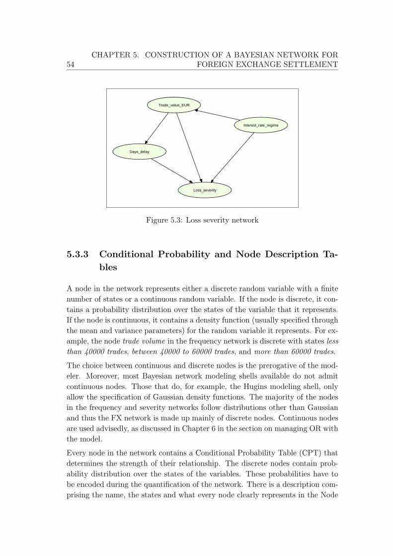
54CHAPTER 5. CONSTRUCTION OF A BAYESIAN NETWORK FOR
FOREIGN EXCHANGE SETTLEMENT
Trade_value_EUR
Interest_rate_regime
Loss_severity
Days_delay
Figure 5.3: Loss severity network
5.3.3 Conditional Probability and Node Description Ta-
bles
A node in the network represents either a discrete random variable with a finite
number of states or a continuous random variable. If the node is discrete, it con-
tains a probability distribution over the states of the variable that it represents.
If the node is continuous, it contains a density function (usually specified through
the mean and variance parameters) for the random variable it represents. For ex-
ample, the node trade volume in the frequency network is discrete with states less
than 40000 trades, between 40000 to 60000 trades, and more than 60000 trades.
The choice between continuous and discrete nodes is the prerogative of the mod-
eler. Moreover, most Bayesian network modeling shells available do not admit
continuous nodes. Those that do, for example, the Hugins modeling shell, only
allow the specification of Gaussian density functions. The majority of the nodes
in the frequency and severity networks follow distributions other than Gaussian
and thus the FX network is made up mainly of discrete nodes. Continuous nodes
are used advisedly, as discussed in Chapter 6 in the section on managing OR with
the model.
Every node in the network contains a Conditional Probability Table (CPT) that
determines the strength of their relationship. The discrete nodes contain prob-
ability distribution over the states of the variables. These probabilities have to
be encoded during the quantification of the network. There is a description com-
prising the name, the states and what every node clearly represents in the Node

CHAPTER 5. CONSTRUCTION OF A BAYESIAN NETWORK FORFOREIGN EXCHANGE SETTLEMENT 55
Description Table (NDT)as given in Tables 5.2 and 5.3.
The idea behind the NDT is to avoid any ambiguity in the meaning of the node.
This is to prevent experts from assigning their own possibly different meanings
and interpretations during the elicitation process. For example, the node front-
office-system has three states: proper functioning (available and working cor-
rectly), malfunctioning (system errors, slow down, or working incorrectly), and
not available or down. The accompanying description reads– the node refers to
the availability and correct working of the front office. The proper functioning of
this system implies the use of Straight Through Process (STP). Not available, or
down, implies the use of manual methods to transmit the trade. The interface
between the front-office-system and the back-office-system is considered part of
the back-office-system.

56CHAPTER 5. CONSTRUCTION OF A BAYESIAN NETWORK FOR
FOREIGN EXCHANGE SETTLEMENT
INTERBANK SERVICES
Frequency Nodes Node Name
Node Description States
Trade volume
Refers to the volume of trade transacted per week. Less than 40,000 40,000 to 100,000 More than 100,000
Frontoffice_system
Refers to the availabil ity and correct working of the front officesystem. Proper functioning implies use of STP and not available or down implies manual transmission or intervention. The interface between frontoffice_system and backoffice_system is considered part of frontoffice_system.
Proper functioning (available + working correctly) Mal functioning (system errors, slow down or working incorrectly) Not available/down
Backoffice_system_slow_downtime
Backoffice_system downtime comprises both slow and downtime before some major currency cut off times. The slow down time are the uncontrolled ones. Controlled ones are not considered here.
Less than 5 minutes (includes non downtime) 5 to 30 minutes ( slow time, downtime, unavailable or working incorrectly) More than 30 minutes.
Backoffice_system_ fail time Refers to the time of backoffice_system failure. Failure can occur at a critical time (some hours or minutes) before cut off times of some major currency or non critical time.
Not Critical Critical
Trade Capture
Refers to whether trade input was done in a correct and timely manner or incorrectly or untimely. Errors include wrong counterparty, wrong side of trade, value date, and rate.
Correct + timely Incorrect or untimely
SSI_in place Whether there is a Standing Settlement Instruction in place or not.
Yes No
Trade type
Whether trade is of type standard or non standard Standard (Spot, Forward, Swaps) Non standard (Options, NDFs etc)
Gross or Netting Refers to whether trade transactions are to settle Gross or should be Netted
Gross Netting
Confirm matching Deals with the activity of confirmation matching before trades are settled. Note, if SSIs are in place, confirmation matching is done automatically and if not in place they are done manually, which may introduces some errors.
Not done (not sent, sent with no feedback etc) Done incorrectly (especially those done manually e.g. phone etc) Done correctly (matched)
Quality of SI Refers to the ratio of Settlement Instructions which are correct and current to the total number of settlement instructions for a typical week.
Excellent (100%) Average (98-100%) Bad (less than 98%)
Paymentsystem_input_ method Refers to the method (manual or automatic) of trade payment instruction input into the paymentsystem after they have been processed.
Straight Through (STP) Manual
Trans_paymentsystem Refers to whether transmission to paymentsystem was done correctly or incorrectly
Correct and timely Incorrect or untimely
Vulnerability to failure Refers to the level to which a trade is liable to fail. It depends on the trade capture and confirmation matching.
Low Medium High
Fails settlement Number of settlement failures in a typical week. Failure here means delays, wrong payments, misdirected payments, non payments and duplicate payments. It depends on the vulnerability to failure, quality of SI, and the input method into the transmission system
0 1 2 3 4 “ “ 16 17
Table 5.2: Node description table - frequency of failures

CHAPTER 5. CONSTRUCTION OF A BAYESIAN NETWORK FORFOREIGN EXCHANGE SETTLEMENT 57
INTERBANK SERVICES
Loss Event Severity Nodes
Node Name
Node Description States
Trade value Refers to the value (amount in EUR) of a trade transaction.
Less than 200,000 200,000 to 500,000 500,000 to 1 mill 1 mill to 5 mill 5 mill to 10 mill 10 mill to 50 mill 50 mill to 100 mill 100 mill to 500 mill 500 mill to 2000 mill
Days delay Refers to the days of delay in re-settling a trade transaction after it has failed.
1 day 2 days 3 days 4 days 5 or more days
Interest rate regime Refers to the environment in which the trade is to settle. The amount of compensation that has to be paid depends on the settlement environment.
USD, Euro zone, GBP, JPY, CHF,etc
Loss severity Refers to the severity of losses attributed to and payment processing failures. This amount is given in EUR.
Less than 1,000 1,000 to 5,000 5,000 to 10,000 10,000 to 50,000 50,000 to 100,000 100,000 to 250,000 250,000 to 500,000 500,000 to 750,000 750,000 to 1 mill 1 mill to 5 mill More than 5 mill
Table 5.3: Node Description Table - severity of losses
5.3.4 Model Structure Validation
After the structure of the model has been determined, the model needs to be
validated structurally. Two approaches are available for use 1) structural valida-
tion with experts and 2) structural validation due to Lauritzen et al.’s (1990) set
theory or due to Pearl’s (1988) d-separation principles (see Chapter 4).
Validation with the experts was carried out in an iterative process. Nodes were
added and deleted during the process until some agreement was reached between
the experts and the modeler that the model was an accurate reflection of the
settlement process. Structural validation according to either the set theory or d-
separation principle was not carried out here. This is because there is a built-in
independence assumption, since the network was modelled in terms of causalities
(causal network). Since the parents of the network were selected as direct causes
of a given variable the local conditional independence conditions are automatically

58CHAPTER 5. CONSTRUCTION OF A BAYESIAN NETWORK FOR
FOREIGN EXCHANGE SETTLEMENT
satisfied (Pearl and Russel, 2001).
5.4 Quantifying the Network
In general a combination of both subjective and objective is used in quantifying
BNs. The emphasis here however, is on subjective data, since the historical data
available was either found to be insufficient, unavailable or not in a form that can
be easily encoded into the networks for some of the nodes. Subjective data was
used for the entire frequency network although the terminal node, fail settlement
has some objective data available. This data was set aside and later compared
to the posterior probabilities of the terminal node during the model validation
process. On the other hand, the severity network was quantified with objective
data, with the exception of the days delay node, which had no historical objective
data available. The objective data used and the process of obtaining subjective
data are described in the next sections.
5.4.1 Objective Data
The structure of the severity network shows that the terminal node, loss severity
depends on trade value, interest rate regime and days delay. The nodes trade value
and interest rate regime are encoded directly with data from the trading books.
The raw data consists of about 40,000 individual trades and 23 significantly dif-
ferent trading currencies, representing a trading period of one week. Details of
these data include the trade date, value date, buy currency, buy amount, and sell
currency. For confidential reasons, the raw data set is not provided in the Ap-
pendix. Processing of these data for final encoding into the network is described
in Section 6.4.2.
Data for encoding the terminal node, loss severity was not directly elicited from
the experts, but was computed according to European Interbank Compensation
Guidelines (European Banking Federation, 2001). The reason is that during the
testing of the elicitation process, the test expert actually computed the various
losses quantities in accordance with European Interbank Compensation Guide-
lines. It was thus deemed reasonable that the experts be spared this enormous
task, when the same computations could be done by the modeler. Details of this
computation is also given in Section 5.5.3

CHAPTER 5. CONSTRUCTION OF A BAYESIAN NETWORK FORFOREIGN EXCHANGE SETTLEMENT 59
5.4.2 The Elicitation Process
Probability elicitation, as already mentioned in Chapter 4, is the process of ob-
taining estimates from domain experts. Our entire bayesian network requires
about 11,155 individual probabilities. Fortunately, about 10,500 probabilities
belonging to the severity network, are from the trade data (objective data) ob-
tained from the trading books. The remaining probabilities (about 650) had to
be elicited from the experts. These probabilities comprise both marginal and
conditional probabilities.
Eliciting conditional probabilities is more difficult, especially if the probability is
conditioned on several states. By applying the principle of divorcing of parents
due to Olesen et al. (1989), described in Chapter 4, the number of states that
the probabilities are conditioned on was reduced, which thus made the process
easier for the experts. It should however be pointed out that in as much as
divorcing parents and introducing intermediate variables lessens the difficult in
eliciting conditional probabilities, it also increases the number of probabilities to
be elicited.
A combined application of parametric elicitation, sensitivity analysis and removal
of weak dependencies (see Chapter 4 for details) was able to further reduce the
number of probabilities to be elicited from 650 to about 190. The use of paramet-
ric elicitation alone, for example, reduced the initial number of estimates from
486 to 27 for the terminal node, fails settlement of the frequency network. Sen-
sitivity analysis uncovered the nodes days delay, quality of SI and vulnerability
to failure as the most influential nodes of the severity and frequency networks
respectively. A greater emphasis was therefore placed on these nodes during the
elicitation process.
The elicitation of expert judgement followed a process which includes designing
the instruments and procedures, testing of the instrument, conducting the real
elicitation and finally editing and validating the estimates elicited. The compo-
nents of the elicitation process are described below.

60CHAPTER 5. CONSTRUCTION OF A BAYESIAN NETWORK FOR
FOREIGN EXCHANGE SETTLEMENT
5.4.3 Protocol, Instruments and Procedures
This subsection describes the protocol followed and the instruments used in our
elicitation.
Protocol
The protocol used, referred to as Composite Protocol is a combination of some
elements of the Stanford or SRI, Morgan and Henrion, Wallsten/EPA, and Cooke
and Goosens protocols presented in Chapter 4. The Composite Protocol was
formulated in order to have a comprehensive protocol that details out the various
steps involved from start to end of the entire elicitation process. The essential
elements are as follows:
• Identification and selection of experts (those for dry run and those for the
real run),
• Preparation of a document that outlines the objective of the process and
motivating the expert with the aims of the elicitation process,
• Structuring the uncertain quantities in an unambiguous way,
• Description of cognitive heuristics, biases and other relevant issues. The
expert reads the document before the elicitation process.
• Definition of elicitation format document describing the exact questions and
format for the expert’s elicitation
• Dry run exercise describing the try out of the elicitation format document
to a few experts ( This dry run may not foresee all the problems. However,
since all in-house experts may share the same view, it is likely to bring out
some interesting issues, which can be addressed during the real run)
• Expert training sessions describing the ingredients of training experts in
preparing probabilistic assessments (describing for example, the elicitation
technique and the quantities to be elicited)
• Expert elicitation sessions
• Feedback communication with the experts
• Documentation of the results

CHAPTER 5. CONSTRUCTION OF A BAYESIAN NETWORK FORFOREIGN EXCHANGE SETTLEMENT 61
Questionnaire
The main component of the instrument used in the elicitation process is a paper
based questionnaire that was developed specifically for this purpose. Certain
decisions were made prior to designing the elicitation questionnaire. One such
decision is the type of information to be collected and the form (response mode)
in which the experts’ answers should be given. The type of information to be
collected could be answers only, or answers plus the problem solving process. Our
questionnaire collects answers only together with ancillary expert data since this
is enough to encode our Bayesian network. Issues regarding the respond mode is
discussed later in this section.
Another decision is whether simple probabilities or parametric distributions should
be elicited. A combination of both was used. Simple probabilities were elicited
for nodes where the burden on the experts was deemed to be minimal. Paramet-
ric distributions on the other hand was elicited for nodes where the burden on
the experts was judged to be heavy. This is against the background that para-
metric elicitations is able to reduced the number of probabilities to be elicited
drastically (see Section 5.4.2). Parametric distributions elicitation is usually used
when the nature of quantities to be assessed suggest they follow a particular class
of probability distributions. As indicated earlier in this section, parametric dis-
tribution elicitation is used for the terminal node of the frequency network. Here
we assumed the ”number of failures” follow a Poisson distribution and thus the
parameters of this distribution were elicited. The assumption of Poisson distri-
bution conforms to the industrial practice of describing the number of failures
with either a Poisson or a negative binomial distribtion.
Having made these decisions, the questionnaire is developed to follow a structure
which is consistent with the composite protocol. The questionnaire comprises the
following elements: introduction; interview information; questions and answers
or response mode; and experts background or ancillary information. These are
described below.
Introduction and Interview Information
The introduction covers the purpose and objective of the elicitation exercise, de-
tails and instructions of the task for the experts and an explanation of the concept
of cognitive heuristics and biases, and motivational biases. A typical introduction
used for our elicitation is given in Appendix A. Interview information included
the date of the interview, the place where the interview took place, the duration
of the interview, and lastly, a description of the interview environment. Experts’
ancillary information was also collected at the concluding part of the question-

62CHAPTER 5. CONSTRUCTION OF A BAYESIAN NETWORK FOR
FOREIGN EXCHANGE SETTLEMENT
naire. This information deals with experts’ background such as job position, the
nature and type of work, previous work experience and how long the expert has
been working at the present job.
The Response Mode
In the field of decision analysis, there are various methods for eliciting proba-
bilities from experts. These methods include probability scales for marking as-
sessments, frequency formats and gambles (see Morgan and Henrion, 1990; von
Winterfeldt and Edwards, 1986). One method found particularly suitable in this
context was that developed by van der Gaag et al. (2002) for eliciting probabili-
ties in a cancer diagnosis study. This method was adopted, modified and used for
this study. It combines ideas such as transcribing the probabilities to be assessed
as fragments of text and providing a scale with both numerical and verbal an-
chors for marking the assessments. The fragments of text are stated in terms of
likelihood rather than in terms of frequency, to prevent difficulties in assessments
for conditioning context that is quite rare. The vertical response scale, with both
numerical and verbal anchors is placed next to the fragment of text. Probabilities
from the same conditional distribution are grouped together so as to encourage
the experts to consider them simultaneously during the elicitation process.
One particular modification made to this method was to format the fragements
of text (questions) so that contrasts among various variable states of a particular
node becomes obvious. This helps the experts to clearly see the differences in
change of state and thus to enable them to give appropriate answers. In addition,
the format is such that similar themes are grouped at the top and the changing
contrast are put at the bottom. The idea is to prevent wearing out the experts
with too much reading load since reading the same scenario before answering
every question on the same node would be repetitive, which might cause fatigue
and irritation. Figure 5.4 gives an example of a typical questionnaire format.

CHAPTER 5. CONSTRUCTION OF A BAYESIAN NETWORK FORFOREIGN EXCHANGE SETTLEMENT 63
This section comprises two sheets – S1 for the state “ not critical” and S2” for the state “ critical” . Please spread both sheets on your table and read all four questions before giving your answers. Not Critical Time
Payment details can be transmitted from the Back office system to the Payment transmission system either Straight Through (auto) or through manual input. Consider a typical working day, where the Back office system has experienced a slowdown or failure at a time that is not critical and the duration of the slowdown or failure is less than 5 minutes. How likely, is it that trade payment details will be input STP into the payment transmission system?
manually into the payment transmission system?
100
85
75
50
25
15
0
Certain (almost)
(almost) impossible
probable
expected
Fifty-fifty
uncertain
improbable
100
85
75
50
25
15
0
Certain (almost)
(almost) impossible
probable
expected
Fifty-fifty
uncertain
improbable
Transmission_payment system_ method (S1)
Figure 5.4: Typical questionnaire format
A further modification made was the use of a matrix format for nodes having
several probabilities from the same conditional distribution. Samples of the ma-
trix format are provided in Appendix A. The matrix table essentially contains
questions covering all probabilities from the same conditional distribution and
the various scenarios for a particular node. The advantage of the matrix format
is that it gives the experts a one shot look at all the probabilities to be elicited
from the same conditional distribution and the different scenarios. This affords
them the opportunity to easily make comparisons among the various scenarios
and to review their estimates without the difficulty of having to turn pages back
and forth. Indeed, the test expert found this approach easier to use and recom-
mended it for the real run.

64CHAPTER 5. CONSTRUCTION OF A BAYESIAN NETWORK FOR
FOREIGN EXCHANGE SETTLEMENT
The matrix format was used for eliciting both point probabilities and probability
distributions. Examples of the format is also given in Appendix A. For the
elicitation of probability distributions, experts were asked to estimate a typical
value and a range within which the typical value falls. An explanation of the
terms typical value and range was provided on the matrix sheet. The typical value
was interpreted as the frequently occurring number, and the range as the 5th and
95th percentile. Experts were also asked to give their estimates in absolute values
instead of percentages. This was to cater for the difficulties and inherent errors in
estimating small probabilities. For example, on average, 2 out of the 8000 daily
number of trades fail. It would have been much more difficult for the experts to
have quantified the corresponding probability of a trade failure, namely 0.00025.
5.4.4 Conducting the Elicitation
Conducting the elicitation involved testing the elicitation procedure, doing the
real run and countering bias during the real run. Experts had to be selected both
for the testing and real run. The elicitation situation and mode of communcation
also had to be defined.
Three experts with considerable experience and training in the domain were iden-
tified. One of the experts was used for the test run and the other two for the real
run. These two experts provided estimates for FX and MM settlement networks
separately. An expert is a person who has background in the subject area and
is recognized by his or her peers, or those conducting the study, as qualified to
answer questions. Questions are usually posed to the experts because they cannot
be answered by other means. The experts’ judgement is more than a guess. It is
an informed opinion, based on the expert’s training and experience (Meyer and
Booker, 2001).
The elicitation situation adopted was a mixture of individual and interactive
group. Individual because the two experts interviewed at the same time worked
on separate networks and were also allowed to interact with each other. Personal
interview (face-to-face) was chosen as the mode of communication in preference
to mail or telephone. This mode was considered best for clarifying some ambi-
guity or misunderstanding with respect to some of the questions asked. Indeed,
some modification was made to the structure of the network during the personal
interviews because the experts found some variables difficult to quantify. This al-
ludes to some of the advantages of doing personal interviews where such issues can
be clarified and settled immediately. Mail or distant interviews do not afford that.

CHAPTER 5. CONSTRUCTION OF A BAYESIAN NETWORK FORFOREIGN EXCHANGE SETTLEMENT 65
Testing
The purpose of the test run is twofold: to obtain feedback information that can
be used to revise the real elicitation and to give training to the project personnel
(elicitor). Testing was carried out on one expert as mentioned earlier. Three
components of the elicitation process were tested. These are introduction given
to the experts, the elicitation procedures, and lastly the entry of data into the
model for analysis or end use.
The first component familiarized the experts with the general steps and schedule
to be followed, the questions and problems to be addressed, the response scale to
use and the biases to which they may be prone. The second was to establish the
duration for the elicitation, the appropriateness of the communication mode, the
ease of understanding of the response mode, the clarity of the questions and the
overall structure of the elicitation procedure among others. The last component
was used to rehearse the entry of the collected data into the model. It also
specifically revealed whether there was any discrepancy between the form of the
elicited data and that necessary for the model.
A few observations made during the test run are: the need to give some form
of training to the experts with regards to estimating probabilities and the use of
the matrix format response mode; the need to provide clear and unambiguous
meanings to some probabilities associated with certain nodes, which the test
expert found difficult to estimate. This led to some nodes being modified or
deleted outright. It was also observed that the test expert guessed probability
estimates for sections where the expert’s knowledge was limited.
The test expert had some initial difficulty with the matrix format, especially in
formulating the questions in each cell. The test expert however, noted that with
some initial training this format would be convenient, accurate and easy to use,
since it emphasises the contrast in each scenario easily. Interestingly, it was ob-
served that the expert was anchoring his estimates on recent events. This is not
however a problem with the design of the elicitation process per se but an issue
of anchoring bias. These observations were addressed during the real run.
Real Run
The real run consisted of six interviews scheduled over a period of eight weeks.
Each interview lasted approximately 2 hours and focused on a small coherent
part of the Bayesian network. The first interview was considered as a training
session, which gave an introduction to the entire elicitation process and allowed
the experts to work on sample questions. Working on sample questions made

66CHAPTER 5. CONSTRUCTION OF A BAYESIAN NETWORK FOR
FOREIGN EXCHANGE SETTLEMENT
use of the element of learning in the sense that an expert would understand a
technique much better after having used it once or twice in the assessment of
different probabilities.
The training session reviewed the network and its probability tables, the basic
ideas underlying the elicitation method (assessment techniques), the basics of
probability theory, and the concept of bias and its effect on the results. Although
the experts had been involved in the construction of the network structure, it was
necessary to go through the network and its probability tables with them again.
The general format of the fragments of text of the questions, the intended use of
the response scale (marking of answers and writing of estimates), as well as the
matrix format of questions were explained and demonstrated to the experts. The
experts were also instructed to simultaneously take into account the different
probabilities of the various states belonging to the same node when providing
their estimates. In addition, they were also made aware of the fact that the
elicitation is not only concerned about events that have occurred before but also
about potential events that can occur under the described scenarios. Finally, they
were informed that their estimates would be subject to analysis that will reveal
the sensitivity of the network behaviour and if necessary the most influential
probabilities will be refined later.
The subsequent interviews were quite straightforward. Each started with a short
briefing by the elicitor and a reading of the introduction by the experts. The pur-
pose was to help the experts refresh their memories about the elicitation process.
Experts were then asked to mark the response scale and write a number close
to their marks or to fill in the spaces provided where appropriate. The process
was interactive with considerable dialogue between the experts and the project
personnel, especially in sections where clarifications were needed. For those sec-
tions, where experts had limited information, they were encouraged to ask for
help from other colleagues.
Bias and Counters
Bias, as mentioned in Chapter 4 is a deviation from reality or what we consider
desirable. If not monitored and controlled in an elicitation process it can have an
impact on the credibility of a project. Some bias tendencies can be anticipated
before the process begins while others occur during the elicitation. Either way,
both have to be monitored and countered. Bias was countered by following a
protocol by Meyer and Booker (2001). The protocol has the following elements:
1) anticipate which biases are likely to occur in the planned elicitation processes,
2) redesign the planned elicitation to make it less prone to the anticipated bi-
CHAPTER 5. CONSTRUCTION OF A BAYESIAN NETWORK FORFOREIGN EXCHANGE SETTLEMENT 67
ases, 3) make the expert aware of the potential intrusion of particular biases and
familiarize them with the elicitation process, 4) monitor the elicitation process
for the occurrence of biases, 5) adjust in real time to counter the occurrence of
biases, and 6) analyse the data for the occurrence of particular biases. However,
not all these elements were needed.
Biases considered relevant to this work were Motivational and Cognitive (incon-
sistency, availability and anchoring). Motivational bias is driven by our human
needs. This was anticipated and countered during the introduction stages by
repeatedly assuring the experts that their answers would neither be subjected
to scrutiny by supervisors, nor would they be used against them in anyway.
Inconsistency may be due to fatigue leading to a faulty memory. To counter
inconsistency, frequent breaks were scheduled during each interview session. In
addition, definitions and assumptions used in the elicitation process, as well as
the response scale, were reviewed at the start of each session. The presentation of
questions and information in our questionnaire was structured hierarchically so
that questions flow from general to the specific. This strategy, which stimulates
and fires the experts memory associations (see Meyer and Booker, 2001) was used
to counter availability bias.
Anchoring bias, the tendency to start with a first impression and then make
only minor adjustments, was dealt with in three different ways: 1) experts were
asked about extreme judgements before obtaining likely ones (see Cleaves, 1986),
2) experts were occassionally asked to describe how other experts might disagree
with their responses, and 3) experts were asked to temporarily forget about recent
events (see Boose and Shaw, 1989). Consistently asking experts to temporarily
forget about recent events was found effective in dealing with the problem of
anchoring responses on recent events. The experts found this approach very
helpful.
5.4.5 Validating the Estimates
It is a known fact that validating an expert’s opinion is a difficult thing to do.
Any attempt should first seek to answer the question ”what exactly do we intend
to validate?” Is it to see 1) whether the elicited probability is the same as or
close to the objective probability that is unknown, or 2) whether the elicited
probability given by the expert is the same as the expert’s knowledge?
There is a fundamental problem in attempting to address the first question. This
is due to the fact that there is no objective distribution or probability to be esti-

68CHAPTER 5. CONSTRUCTION OF A BAYESIAN NETWORK FOR
FOREIGN EXCHANGE SETTLEMENT
mated. The implication is that a particular subjective probability or distribution
cannot be judged to be true or untrue, except of course, in some extreme cases
where elicited probabilities are just unreasonable. One attempt in the literature
(see Lindley et al., 1979) to deal with this problem requires that there be an
objective assessor who will consolidate the results derived from the subjective
experts. This model is currently being used by several banks in their operational
risk self assessments, where the line manager provides probability estimates and a
superior to the line manager, or the internal audit (assessor), validates the self as-
sessments. The problem, however, with this approach is the implied assumption
that the assessor is more objective than the expert.
The writer agrees with the opinion of Kandane and Wofson (1998) that since
elicitation purports to represent the opinions of the person being elicited, and
only that, any attempts at validation should use only other statements of belief
by that person as data. A compromise to the method of elicitor and objective
assessor, which seems useful is to elicit a quantity from a number of experts
and then to aggregate these quantities into a single estimator and corresponding
distribution through Bootstrap sampling and simulation (see Meyer and Booker,
2001). This is based on the premise that more than one person is a repository
of the knowledge within a particular domain that is being elicited. This model
unfortunately, can not be implemented if there are only a few experts in the
domain being investigated, as was in the case study described here. However,
a comparison of the estimates obtained from the two experts in the case study
showed a high degree of consistency.
In OR self assessments, it is widely believed that experts may for obvious reasons,
underestimate the frequency and severity of losses. This belief then transforms
the problem of how close the elicited probability to the objective probability to a
question of managing motivational bias - how can line managers be motivated to
give a true and objective assessment of their risk? Managing motivational bias is
therefore seen as a way to improve the quality of probabilities elicited, especially
in operational risk. Managing motivational bias has already been addressed in
earlier sections.
The question on whether probabilities elicited from the experts are the same as
the expert’s knowledge was dealt with by using the elements of validation (co-
herency, consistency and reliability checks) mentioned in Chapter 4. The specific
approach used was to confront the experts with their estimates. Confronting the
experts periodically with their answers for each coherent section of the network
helps check the consistency or coherency and reliability of their estimates. This
allows the experts to compensate for their natural biases and ensures the reli-

CHAPTER 5. CONSTRUCTION OF A BAYESIAN NETWORK FORFOREIGN EXCHANGE SETTLEMENT 69
ability of the estimates by way of the experts giving their overall statement of
satisfaction. The approach is similar to the user-friendly JAVA interface created
by Lau and Leong (1999), that checks possible biases and any inconsistencies in
elicited probabilities by entering into dialogue with the expert until consistency is
achieved. Besides confronting the experts with their estimates, the overall math-
ematical and statistical consistency (for example, probabilities adding up to one)
of the estimates were also checked by the elicitor.
5.5 Data Processing
The data elicited from the experts, as well as those collected from historical
sources had to be put in a form that can be encoded into the Bayesian network.
This section describes how the data was prepared. It first looks at the data used
for the frequency network and later that used for the severity network.
5.5.1 Frequency Data
As indicated earlier, expert judgement was elicited for all nodes in the frequency
network. The quantities elicited include both probability estimates and para-
metric distributions (see Appendix B)1. The probability estimates were directly
encoded into the frequency network. This is possible because the questionnaire
were structured on the basis of the network.
The parametric distribution elicited for the terminal node (frequency of failure)
has to be transformed before encoding into the network. To carry out the trans-
formation, some assumptions were first made - the number of failures is assumed
to follow a Poisson distribution and also our typical value is interpreted as the
mean of the assumed Poisson distribution. This assumption is consistent with in-
dustrial practice and studies in operational risk that show that number of failures
usually follow either a Poisson or Negative binomial distribution. The Poisson
distribution is chosen over the negative binomial because the negative binomial
was found to be overly dispersed for the elicited data (typical value, and the 5th
and 95th percentile).
A Poisson distribution has only one parameter, λ (mean) and it is not always pos-
sible to satisfy both conditions of a prescribed mean and the two elicited quantiles
(5th and 95th). It is however, possible to satisfy the condition of a prescribed
1the elicited data presented in Appendix B has been transformed for confidentiality reasons

70CHAPTER 5. CONSTRUCTION OF A BAYESIAN NETWORK FOR
FOREIGN EXCHANGE SETTLEMENT
mean and one quantile by dropping the exactness requirement and using a con-
dition ”as close as possible” with respect to a predefined metric by determining
λ0 such that
A ∗ (λ− λ0)2 + B ∗ (P (Xλ0 > Y )− 95%)2 is minimized.
A and B are weights emphasising the importance of the mean and the quantile
value. Y is the value that corresponds to the 95 % quantile.
An application of this condition with various weights to the elicited data showed
that the result is not very different from simply fitting a Poisson with its λ equal
to the typical value without any conditions (placing all emphasis on λ). The
insignificant difference may be due to the fact that our data is somehow ”under
dispersed”. This is true upon critical examination. Placing of full emphasis on
the typical value is also consistent with the fact that when faced with the task of
estimating statistics intuitively from data, subjects have been shown to be fairly
accurate at guessing values of central tendency but not the variance of the data
(Spencer, 1963; Swanson, 1966).
Having fitted a Poisson distribution to the elicited data, the various probabili-
ties as specified in network were computed and encoded into the network. Some
Bayesian network modeling shell (for example Hugins Expert) allows the specifi-
cation of parameters of known distributions. This significantly lessens the burden
on the modeler. The prior probabilities used for encoding the network are given
in Appendix B2.
5.5.2 Loss Severity Data
The historic data used for encoding the severity network consists of trade infor-
mation for 23 significantly different trading currencies. The various trade values
were first converted to one common currency, the Euro (EUR), using the ex-
change rate that prevailed at each individual trade date. Data preparation for
each of the individual nodes (days delay, interest rate regime, trade value and
loss severity) are given below.
2the prior probabilities presented in Appendix B has also been transformed for confidentialityreasons

CHAPTER 5. CONSTRUCTION OF A BAYESIAN NETWORK FORFOREIGN EXCHANGE SETTLEMENT 71
Interest Rate Regime
Each trade in the data base has two sides; a buy side and a sell side. The sell
side currency is the currency that has to be delivered and settled. The interest
rate prevailing at the country where the sell side currency has to settle is chosen
as the interest rate regime. For example, a trade with buy side EUR and sell side
US dollar (USD) is represented as USD and is assumed to settle in the United
States of America with its corresponding interest rate. Currencies that have some
similarities in their exchange rate to the EUR and interest rates were grouped
together and their interest rate was represented by a weighted average. Examples
are the Australian dollar (AUD) and New Zealand dollar (NZD) represented as
AUD/NZD and the the Russian rubble (RUB), Czeck krone (CZK) and the
Swedish krone represented as RUB/CZK/SKK. The representative interest
rates were obtained from the internet websites of the corresponding Central Banks
posted on 21.08.04. Table 5.4 shows the probability distribution of the various
currencies and their interest rates.
Currency Percentage share
Interest rate (%) as at 21.08.04
USD 37.95 2.000 EUR 28.22 3.000 JPY 9.62 0.002 GBP 7.61 4.750 CHF 5.05 2.000 AUD/NZD 2.62 5.375 CAD 1.83 2.000 RUB/CZK/SKK 1.04 3.267 SGD 1.02 1.100 SEK 0.84 2.750 NOK 0.69 1.750 TRL 0.67 25.000 PLN 0.63 6.000 HKD 0.49 3.000 HUF 0.46 18.000 DKK 0.33 2.200 ZAR 0.29 7.500 MXN 0.15 7.100 BRL 0.07 16.000
Table 5.4: Currency distribution and interest rates

72CHAPTER 5. CONSTRUCTION OF A BAYESIAN NETWORK FOR
FOREIGN EXCHANGE SETTLEMENT
Trade Value
To encode the various trade values into the network, the probability distribution
of each currency was first determined. Two approaches were possible; use of
parametric or non-parametric methods. Both methhods have their advantages
and disadvantages. The later approach was used since the various trade values
have fat tails and it was found expedient to let the data speak for itself, especially
at the tails. An exploratory data analysis is given in Figure 5.5. Kernel density
methods were used to estimate the various densities.
Histogram of EUR trades on logscale
Log of trade values
Den
sity
0 5 10 15 20
0.00
0.10
0.20
0.30
Histogram of NOK trades on logscale
Log of trade values
Den
sity
5 10 15
0.00
0.10
0.20
Histogram of HKD trades on logscale
Log of trade values
Den
sity
5 10 15
0.00
0.05
0.10
0.15
Histogram of BRL trades on logscale
Log of trade values
Den
sity
13.0 14.0 15.0 16.0
0.0
0.4
0.8
Figure 5.5: Exploratory graphs of some trade values
Kernel Density Estimates
In kernel density estimation there is always the issue of bias-variance trade off that
has to be addressed. Two components that significantly affect this trade off are
the bandwidth and the degree of local polynomial used. If the chosen bandwidth
is too small, insufficient data will fall within the smoothing window and a large
variance will result. If it is too large, some important features of the data may
be distorted or lost. For any estimation problem, one may decide to either 1)
apply a constant bandwidth to all observations, 2) choose a separate bandwidth

CHAPTER 5. CONSTRUCTION OF A BAYESIAN NETWORK FORFOREIGN EXCHANGE SETTLEMENT 73
for each fitting point or, 3) use a nearest neighbour bandwidth. Option two and
three are classified as adaptive bandwidth selection.
A constant bandwidth for all fitting points is the simplest approach. Although
simple, it may lead to problems of empty neighbour, which is most severe in tail
regions. Choosing a separate bandwidth for each fitting point (see Brewer, 2000)
is therefore preferable but computationally expensive, especially with numerous
data points . The use of nearest neighbourhood bandwidth (see Loader, 1999)
ensures that local neighbourhood always contains a specified number of points
(solves the problem of empty neighbour) and also assigns different bandwidths to
neighbourhood of points (adaptive bandwidth selection).
The degree of the local polynomial chosen also affects the bias-variance trade off.
A higher polynomial degree will provide a better estimate, meaning less bias,
but at the same time increases the variability of the estimates since the number
of coefficient to estimate increases. This is in direct opposite to the effect of
bandwidth. Experience shows that it is better to choose a low degree polynomial
and rather concentrate on choosing a bandwidth. A local linear estimate usually
produces a better fit, especially at the boundaries; a local quadratic reduces the
bias but increases the variance, which can be a problem at the boundaries, and
local cubic and higher orders hardly produce much benefit (Loader, 1999).
Application
The distributions of trade values data have fat tails. When the constant band-
width approach was applied to the data set, the problem of empty neighbour
was very pronounced for all the individual currencies with the exception of the
Turkish Lire (TKL)and Brazilian Real (BRL). The use of separate bandwidths
for each fitting point of our data was found to be computationally expensive
(for example, Euro currency has over 17,000 observations). Use of locally adap-
tive fitting methods together with the nearest neighbour bandwidth method (see
Loader, 1999, chp. 11) produced the most satisfactory results for the data set
and was therefore used on all currencies except the TKL and BRL. For these two
the constant bandwidth approach was used with an additional technique of cut-
ting off the negative values of the estimate and rescaling the density to provide a
positive support for the estimates. Figure 5.6 shows some examples of the kernel
density estimates.

74CHAPTER 5. CONSTRUCTION OF A BAYESIAN NETWORK FOR
FOREIGN EXCHANGE SETTLEMENT
0 10 20 30 40 50 60
0.0
0.1
0.2
0.3
MXN (nearest neighbour method)
trade value in millions of EUR
dens
ity
0 20 40 60 80
0.00
0.10
0.20
0.30
ZAR (nearest neighbour method)
trade value in millions of EUR
dens
ity
0 5 10
0.00
0.10
0.20
BRL (constant bandwidth method)
trade value in millions of EUR
Den
sity
0 2 4 6 8 10 12 14
0.00
0.10
0.20
BRL (const bw with cutoff)
trade value in millions of EUR
Den
sity
Figure 5.6: Kernel density estimation
Goodness of fit tests were carried out as follows: For a variety of smoothing
parameters the density was estimated. A graphical comparison was then made
between the empirical distribution function and the integrated density estimates.
The emphasis of the comparison is at the tails, which is of much interest in op-
erational risk. Quantile-quantile (qqplots) of the residuals obtained from the fit
were also examined to assess the extent of lack of fit. For cases where there were
competing models, and in which the graphs did not show clear distinctions, the
Kulbach-Leibler (K-L) empirical discrepancy criteria was used. The essential part
of the K-L empirical discrepancy criteria, which emphasises the fit in the tails of
the density is given as
θ = argmin{− 1n
∑ni=1 log gθ(xi), θ ∈ Θ}
Some examples of goodness of fit tests are shown in Figure 5.7.

CHAPTER 5. CONSTRUCTION OF A BAYESIAN NETWORK FORFOREIGN EXCHANGE SETTLEMENT 75
0.5 1.0 2.0 5.0 10.0 20.0 50.0
0.0
0.4
0.8
Cdf of MXN trades, fitted (step) vrs empirical
trade value in millions of EUR
cum
ulat
ive
dens
ity
−2 −1 0 1 2
1.5
2.5
3.5
Normal Q−Q Plot
Theoretical Quantiles
Sam
ple
Qua
ntile
s
Figure 5.7: Assessing goodness of fit
5.5.3 Loss Severity - Probability Computations
Having obtained the estimated density of the various currencies, the probabilities
needed for encoding the network are computed for the bin sizes pre-defined in
the severity network. The computations are made in particular for two nodes:
trade value and the loss severity nodes. Computations for the node trade value
are quite straightforward (finding the proportional area under the curve covered
by the defined bins) and will not be treated here. Computations of probabilities
for the terminal node (loss severity) are discussed below.
Loss Severity Node
According to the severity network, loss severity depends on the trade value, the
days delay, and the interest rate regime. The loss incurred if a trade fails to settle
correctly, is computed as the product of the trade value, the days delay and the
interest rate pertaining at the interest rate regime all divided by 360 days. This
conforms with the European Interbank Compensation Guidelines (see European
Banking Federation, 2001). Three points from the Guidelines are relevant for the

76CHAPTER 5. CONSTRUCTION OF A BAYESIAN NETWORK FOR
FOREIGN EXCHANGE SETTLEMENT
computations: 1) compensations less or equal to 100 Euros are considered ”de
minimum” and not claimed, 2) an administration cost of 100 Euros is payable for
failed trades and 3) in situations where the product of the trade value and the
days delay is greater or equal to 200 million Euros, the compensation to be paid
can be negotiated between the parties concerned.
The first provision is catered for in the network by cutting off losses less than
100 euros and normalizing the loss distributions. The last two provisions, for
simplicity reasons, are not considered in the model. The interbank FX and MM
market is a highly regulated market, unlike client FX market. As a result, the
principal amount cannot be lost when banks trade with each other. The losses
computed in the model is based on all currencies and corresponding interest rates,
trade values, and an assessment of the days delay for a one-week trading period.
The computed losses can therefore be considered as the universe of all possible
losses that can occur for a one week trading period. The computations of the
probabilities are given below.
Let L represent the Loss severity, Int the interest rate in percentage, V the trade
or monetary value, D the days delay, which takes values d = 1, 2, 3, 4, 5, ... and
k be a value representing Int360∗100
. Further, let, lrL be the lower bound of loss
severity, urL the upper bound of loss severity, lrV the lower bound of trade
value, and urV be the upper bound of trade value. The basic equation is
L = V.D.k (5.1)
According to the severity Conditional Probability Tables (CPT ), we are looking
for
P (lrL ≤ L ≤ urL | lrV ≤ V ≤ urV ) (5.2)
The conditional probability in Equation (5.2) can be expanded to
P (lrL ≤ L ≤ urL ∩ lrV ≤ V ≤ urV )
P (lrV ≤ V ≤ urV )(5.3)
The denominator P (lrV ≤ V ≤ urV ) of equation (5.3) can be computed as
∫ urV
lrV
fv(V )dv. (5.4)

CHAPTER 5. CONSTRUCTION OF A BAYESIAN NETWORK FORFOREIGN EXCHANGE SETTLEMENT 77
and the numerator P (lrL ≤ L ≤ urL | lrV ≤ V ≤ urV ) of equation (5.3) is
expanded as
5∑
d=1
P (lrL ≤ V.d.k ≤ urL ∩ lrV ≤ V ≤ urV | D = d)P (D = d) (5.5)
=5∑
d=1
P (lrL
d.k≤ V ≤ urL
d.k∩ lrV ≤ V ≤ urV )P (D = d) (5.6)
=5∑
d=1
P{max[(lrL
d.k), lrV ] ≤ V ≤ min[(
url
d.k), urV ]}P (D = d). (5.7)
The first part of equation (5.7) can be written as
∫ min(urLd.k
,urV )
max( lrVd.k
,lrV )
fv(V )dv. (5.8)
Putting it all together we obtain the final equation
∫ min(urLd.k
,urV )
max( lrVd.k
,lrV )fv(V )dv
∫ urV
lrVfv(V )dv
.P (D = d). (5.9)
The second part of the final equation P (D = d) is catered for by the way the
CPTs in the Bayesian network is constructed.

78CHAPTER 5. CONSTRUCTION OF A BAYESIAN NETWORK FOR
FOREIGN EXCHANGE SETTLEMENT
5.6 Aggregating the Frequency and Severity Out-
puts through Monte-Carlo Simulation
The Bayesian networks developed produces two set of results (from the terminal
nodes): 1) frequency of failures and 2) severity of losses. These two distribu-
tions are compounded through Monte-Carlo simulations to obtain a potential loss
distribution, which shows the potential losses that can occur in the settlement
process with its likelihood (see Figure 5.8). This section outlines the basic idea
underlying the Monte-Carlo simulations. The results from the Bayesian networks
and the Monte-Carlo simulations are described in Chapter 6.
Figure 5.8: Aggregating frequency and severity distributions

CHAPTER 5. CONSTRUCTION OF A BAYESIAN NETWORK FORFOREIGN EXCHANGE SETTLEMENT 79
The idea underlining Monte-Carlo simulation is rather simple. To start the simu-
lation, a decision is made on the number of iterations, say 100,000. The simulation
proceeds as follows:
1. Generate a number of loss frequencies from the frequency distribution. Let’s
call this number fd[1] for the first iteration.
2. Generate loss severities from the severity distribution for this iteration. The
quantity of loss severity generated should be the same as the number of loss
frequency generated above. That is, if the number of loss frequencies gener-
ated fd[1] is 3, we generate 3 loss severities from the severity distribution.
3. Add up the loss severities generated in 2) above for this particular iteration
4. Repeat the process for the total number of iterations, say 100,000.
Iterations
Loss frequency
Loss severity
Potential loss
1 2 3 . . . . n
1 4 2 . . . .
24.0 12.4 3.7 . . . .
- 17.2 5.3 . . . .
- 3.1 - . . . .
- 25.2 - . . . .
24.0 57.9 9.0 . . . .
Table 5.5: Monte-Carlo simulations
Another way of executing this algorithm is by generating all frequencies and all
the losses separately and later sorting and summing the generated losses into
their various iterations. A random number generator is needed to generate the
frequency and losses from the respective distributions.

80CHAPTER 5. CONSTRUCTION OF A BAYESIAN NETWORK FOR
FOREIGN EXCHANGE SETTLEMENT
5.7 Maintaining the network
The Bayesian network constructed has to be maintained and periodically updated
to reflect current conditions. The network structure and the initial probabili-
ties should be updated periodically. Updating the network structure is particu-
larly useful in operational risk management where the domain drifts over time
(changing control environment and process flow). When the control environment
changes, nodes can be added, deleted or modified to relect the current changes.
New set of probabilities will also have to be elicited for the modified nodes.
Updating the initial probabilities used for encoding the network will require the
establishment of a database based on the network structure. The database should
have the same format as the CPTs so that historical data collected can be readily
encoded into the Bayesian network periodically. In Bayesian networks, periodi-
cally updating the conditional probability distributions for a domain as observa-
tions are made is called sequential updating, adaptation or sequential learning.
One of the most common adaptation algorithms was developed by Spiegelhalter
and Lauritzen (1990), who also introduced the notion of experience. Readers are
referred to Cowell and Dawid (1992) and Olesen et al. (1992) for a mathematical
treatment of adaptation. Experience is central to the process of adaptation. It is
quantitative memory which can be based both on quantitative expert judgment
and past cases. Experience can be formulated to either give equal weights to
recent and older experiences or formulated to consider new observations more
important than older ones and thus given more weight in the adaptation process.
The later process is usually achieved by specifying a fading factor, which is the
rate at which previous observations are forgotten. The algorithms for adaptation
is implemented in most Bayesian network modeling shells.

Chapter 6
Results, Validation and
Applications
6.1 Model Results
The Bayesian network model developed and encoded in Chapter 5 was compiled
to obtain some sample results. Compilation in the Hugin Expert modeling shell
used was achieved through the junction tree algorithm described in Chapter 3.
That is, the BN was first transformed into a junction tree and messages are then
propagated through the tree to obtain the posterior probabilities. This chapter
describes the results obtained from the frequency and severity networks. The
aggregation of these results to obtain a potential loss distribution is also shown
in this chapter. Included in this chapter is the assessment of the performance of
the model. The last part of the chapter shows how the model can be used to
manage operational risk in FX and MM settlement.
6.1.1 Results – Frequency of Failure and Severity of Losses
The frequency network with some posterior probabilities is shown in Figure 6.1.
The probability distribution for the terminal node (hypothesis node) fails set-
tlement shows that for a period of one week, the probability of having no trade
failure is about 11%, one failure is about 23%, two failures is about 24% and
three failures is about 18%. These results are later compared to historical data.
Figure 6.2 shows the severity network with some posterior probabilities. The
distribution of the node of interest, loss severity indicates that the most likely

82 CHAPTER 6. RESULTS, VALIDATION AND APPLICATIONS
Figure 6.1: Frequency network showing some posterior probabilities
loss amount should given a settlement failure in a week is less than 1000 EUR.
The corresponding probability of occurrence is 90%. Other features are lossess of
between 5,000 EUR to 10,000 EUR, 100,000 EUR to 250,000 EUR and 750,000
EUR to 1 million EUR occuring with probabilities of 1.46%, 0.129% and 0.005%
respectively.

CHAPTER 6. RESULTS, VALIDATION AND APPLICATIONS 83
Figure 6.2: Severity network showing some posterior probabilities
6.1.2 Results – Aggregated Potential Losses
A summary of the results obtained from the aggregation through Monte-Carlo
simulation is given in Table 6.1. A histogram of the potential loss is shown in
Figure 6.3. The results indicate that the mean loss that can occur within a trading
week is about 11,290 EUR with a variance of 136 EUR. The maximum potential
loss that can be experienced is 3,142,000 EUR. The potential loss distribution
like the loss severity distribution also has a fat tail.
Min 1st quartal Median Mean
3rd quartal Max
Standard deviation
Model results 0.050 760 1,400 11,300 3,000 3,142,000 130,438
Table 6.1: Summary statistics of potential loss

84 CHAPTER 6. RESULTS, VALIDATION AND APPLICATIONS
Histogram of potential loss
log of potential loss
Den
sity
0 5 10 15
0.0
0.2
0.4
Figure 6.3: Histogram of potential losses
6.1.3 Results – Operational Value at Risk
Value at Risk (VaR) measures the worst expected loss under normal market
conditions over a specific time at a given confidence level. It normally answers
the question how much can be lost with x% probability over a preset horizon (J.P.
Morgan and Reuters, 1996). It is normally denoted as V aR at holding period t
and confidence level 100(1 − α)%. For example, a weekly V aR of 500,000 EUR
at 5% (α = 5%) means only 5 chances in a 100 that a weekly loss bigger than
500,000 EUR occurs under normal market conditions.
Usually when the primary goal is to satisfy external regulatory requirements, the
(α) or quantile is typically very small, for example 1%. However, for an internal
risk management model used by a firm to control its risk exposure, the typical
number is around 5%. In operational risk the regulatory value is fixed at 0.1%,
that is, the confidence level is at 99.9%. Since the FX model is primarily for
management purposes, the operational value at risk (OpVaR) is also evaluated
at 95%. A simple way of computing the OpVaR is to order the values obtained
from the aggregated distribution (Monte-Carlo simulations) in descending order.
The quantiles are then obtained by dividing the position of each value by the
number of runs. Table 6.2 shows some OpVaR values. The significant difference
between the OpVaR value at 99.5% and 99.9% also confirms the fat tail of the
distribution.
The operational risk expected loss is the mean of the aggregated potential loss
distribution and the unexpected loss at the ith percentile is the difference between
the upper ith percentile and the mean of the potential loss distribution. The
expected loss and the unexpected loss at both 99.9% and 95% are given in Table

CHAPTER 6. RESULTS, VALIDATION AND APPLICATIONS 85
6.2. The unexpected loss of 2,823,000 EUR at 0.1% (99.9 quantile) means there
is only a 0.1 chance in a 100 that a weekly loss bigger than 2,823,295 EUR occurs
under normal trading or settlement conditions.
i th percentile Mean Unexpected loss at ith
percentile
95.0 99.5 99.9 - 95.0 99.5 99.9
Loss (EUR)
13,900
175,000
2,834,000
11,300
2,600
163,000
2,823,000
Table 6.2: Operational risk unexpected loss
6.2 Model Validation
The FX and MM settlement model developed is validated through a series of
comparisons carried out in this sections. The model’s output – distribution of
frequency of failure and severity of losses are compared with historical data. The
aggregated potential loss distributions simulated through Monte-Carlo methods
for both the model and historical data are also compared. The historical data
used for the comparison are first described.
Historical Loss Data
The historical loss data used for comparison is actually simulated from a banks
real loss data for FX and MM settlement processes. The simulation was done in
order to respect data privacy laws. It is however believed that the integrity of
the data was somehow kept during the simulation process to enable a reasonable
comparison to be carried out. The data covers a total period of about two years
(2002 - 2004).
The historical data is truncated. As indicated earlier in Chapter five, the Euro-
pean Interbank Compensation Guidelines stipulates that settlement losses less or
equal to 100 Euros are not claimed. This gives a truncation point of 100 EUR.
There are however a few data points with loss values less than 100 EUR found
in the data set. Additionally, the experts indicated during the elicitation process
that at the beginning of the historical data collection exercise, losses less than
1000 EUR where not recorded. This amount was later reduced to 500 EUR at
some point in time. Unfortunately, the time for this change is not documented.

86 CHAPTER 6. RESULTS, VALIDATION AND APPLICATIONS
Thus the dataset could possibly be truncated at 100, 500 or 1000 EUR. To sim-
plify the comparison, the model results are also truncated at 100, 500 and 1000
EUR for the loss severity data before comparing them with the historical loss
data.
6.2.1 Comparison of Results – Frequency of Failures
The frequency of failures from the model results have a weekly time span. In
view of this, the historical frequency of failure data is first regrouped to also have
a weekly time span. For ease of comparison, a Poisson distribution was fitted to
the historical data. The graphical comparisons are shown in Figure 6.4
From Figure 6.4 the chances of experiencing one or zero number of failures in
a trading week are higher for the historical data (about 30 and 40 percent re-
spectively) than for the model results (about 10% and 25% respectively). On
the other hand, the chances of experiencing two or more failures are higher for
the model results than the historical data. Additionally, whereas the probable
number of failures for the historical data terminates at five, that of the model
results terminate at seventeen, but with a small chance of occurrence (0.028%).
These results are not surprising but confirm the fact that the model includes
various scenarios, which might not have occured before but do have the potential
of occurring. An example is the estimation of probabilities for rare events like
the number of failures exceeding 10 failures per week when the historical loss
data has never recorded more than 10 failures per week. Another example is the
estimation of probabilities for the states ”proper functioning”, ”mal function” and
”not available” for the node ”front office system” under the scenario of ”trade
volume” between 100,000 and 150,000. Such a weekly trade volume has never
been recorded in history. These probabilities although small do influence the final
results. The inclusion of such scenario analysis prevents estimating as zero the
inherent operational risk within certain process with little or no available history
of losses (see van den Brink, 2002, chp. 2).

CHAPTER 6. RESULTS, VALIDATION AND APPLICATIONS 87
0 5 10 15
0.0
0.1
0.2
0.3
Historical failures
# of failures
prob
abili
ty
0 5 10 15
0.00
0.10
0.20
Model results
# of failures
prob
abili
ty
0 5 10 15
0.0
0.1
0.2
0.3
Model results vrs historical
# of failures
prob
abili
ty
0 5 10 15
0.0
0.2
0.4
0.6
0.8
1.0
CDF of model vrs hist (step),
# of failures
dens
ity
Figure 6.4: Comparison of frequency of failure
6.2.2 Comparison of Results – Severity of Losses
Comparisons are made for both data sets truncated at 100, 500 and 1000 EUR.
To help with the comparison, a lognormal distribution was fitted to the historical
loss data. Thereafter, a comparison of the commulative density function (cdf) of
the model results and the historic data is made (see Figure 6.5). Furthermore,
quantile-quantile plots (qq plots) of the two data sets (see Figure 6.6) is also
made. The idea behind the qq plot is to first obtain corresponding values of the
same quantiles for both cdfs and later plot them against each other. If both are
comparable, they should follow a 45 degree inclined straight line.
The cdf plots show that losses from our model results are higher than those from
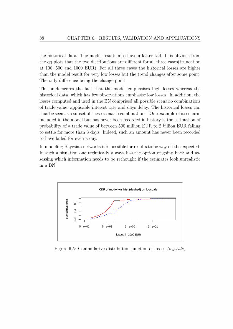
88 CHAPTER 6. RESULTS, VALIDATION AND APPLICATIONS
the historical data. The model results also have a fatter tail. It is obvious from
the qq plots that the two distributions are different for all three cases(truncation
at 100, 500 and 1000 EUR). For all three cases the historical losses are higher
than the model result for very low losses but the trend changes after some point.
The only difference being the change point.
This underscores the fact that the model emphasises high losses whereas the
historical data, which has few observations emphasise low losses. In addition, the
losses computed and used in the BN comprised all possible scenario combinations
of trade value, applicable interest rate and days delay. The historical losses can
thus be seen as a subset of these scenario combinations. One example of a scenario
included in the model but has never been recorded in history is the estimation of
probability of a trade value of between 500 million EUR to 2 billion EUR failing
to settle for more than 3 days. Indeed, such an amount has never been recorded
to have failed for even a day.
In modeling Bayesian networks it is possible for results to be way off the expected.
In such a situation one technically always has the option of going back and as-
sessing which information needs to be rethought if the estimates look unrealistic
in a BN.
5 e−02 5 e−01 5 e+00 5 e+01
0.0
0.4
0.8
CDF of model vrs hist (dashed) on logscale
losses in 1000 EUR
cum
ulat
ive
prob
Figure 6.5: Commulative distribution function of losses (logscale)

CHAPTER 6. RESULTS, VALIDATION AND APPLICATIONS 89
0 200 400 600 800 1000
010
025
0QQplots−truncated at 100
model results (in 1000s)
hist
oric
al lo
sses
(in
100
0s)
0 200 400 600 800 1000
010
025
0
QQplots−truncated at 500
model results (in 1000s)
hist
oric
al lo
sses
(in
100
0s)
0 200 400 600 800 1000
010
025
0
QQplots−truncated at 1000
model results (in 1000s)
hist
oric
al lo
sses
(in
100
0s)
Figure 6.6: QQ plots of losses with truncations at 100, 500 and 1000 EUR
6.2.3 Comparison of Results – Potential Losses
Comparisons are made again for the three truncation points. First the summary
statistics of the two distributions (model results and historical data) are provided
in Table 6.3. These results are obtained through the Monte-Carlo simulations
mentioned in section 6.4 (for the historical data, the simulation is generated from
the Poisson and lognormal distribution fitted to the historical frequency of failure
and historical losses respectively). We compare the cdfs plots on logscale followed

90 CHAPTER 6. RESULTS, VALIDATION AND APPLICATIONS
by a qq plot of the two distributions. The qq plots are broken up into two quantile
ranges so that we do not miss some of the fine features of the plots.
The summary statistics show that for all three truncation cases, the model results
have a higher maximum potential loss, 99.5% and 99.9% quantile values than the
historic potential losses. In addition, the first three quartals (1st, median, 3rd
quartal) of the model results, except the 100 EUR truncated data set are higher
than the historical results. In general, the cdf plots in Figure 6.7 show that the
model results have fatter tails than the historical results. A careful look at the
cdfs of the three truncation cases indicate indicates that the model results and
historical data for truncation at 1000 EUR compares most favourably than the
others. This is not surprising especially when our model emphasises high losses.
Trancation at 100 EUR
Min 1st quartal Median Mean
3rd quartal Max
Standard deviation
99.5 percentile
99.9 percentile
Model results 100 789 1,461 11,570 3,047 3,142,000 132,096 174,753 2,834,584
Historical simulation 100 1038 2,910 7,150 7,493 1,084,000 15,282 71,921 146,771
Trancation at 500 EUR
Min 1st quartal Median Mean
3rd quartal Max
Standard deviation
99.5 percentile
99.9 percentile
Model results 500 825 1,518 13,630 3,363 3,142,000 145,310 174,181 2,834,267
Historical simulation 500 1,557 3,655 8,160 8,660 1,084,000 16,182 71,694 146,771
Trancation at 1000 EUR
Min 1st quartal Median Mean
3rd quartal Max
Standard deviation
99.5 percentile
99.9 percentile
Model results 1,002 2,845 4,598 42,730 11,100 3,142,000 267,342 173,116 2,833,333
Historical simulation 1000 2,190 4,537 9,354 10,000 1,084,000 17,250 71,663 146,771
Table 6.3: Operational risk unexpected loss

CHAPTER 6. RESULTS, VALIDATION AND APPLICATIONS 91
0 5 10 15
0.0
0.2
0.4
0.6
0.8
1.0
CDF−model vrs hist.(dashed), No trunc.
log of losses
cum
ulat
ive
prob
abili
ty
6 8 10 12 14
0.0
0.2
0.4
0.6
0.8
1.0
CDF−model vrs hist.(dashed), 100 EUR trunc.
log of losses
cum
ulat
ive
prob
abili
ty
6 8 10 12 14
0.0
0.2
0.4
0.6
0.8
1.0
CDF−model vrs hist.(dashed), 500 EUR trunc.
log of losses
cum
ulat
ive
prob
abili
ty
8 10 12 14
0.0
0.2
0.4
0.6
0.8
1.0
CDF−model vrs hist.(dashed), 1000 EUR trunc.
log of losses
cum
ulat
ive
prob
abili
ty
Figure 6.7: Potential loss - cdf comparison
The qq plots in Figures 6.8 and 6.9 show that overall (quantile 0 - 1), the model
compares badly with the historical results for all cases of truncation. A detailed
look at quantile plots (quantile 0 - 0.97) however, indicates a better comparison
– meaning the main body of the two distributions up to about the 0.97 quantile
are comparable. The significant difference is really at the tails of the distribution,
where the model results are significantly higher than the historical distribution.
A critical examination of the quantile 0 - 0.97 plots indicate that potential loss
from historical simulation are higher than the model results only up to a par-
ticular loss amount. After this amount there is a change in the trend and the
models results become higher than the historical losses. That is, as one moves
further away from the body of the distribution, the model results become higher
than the historical results. The change points are different for each of the cases,
for example, about 10,000 EUR for truncation at 1000 EUR, 20,000 EUR for
truncation 500 EUR and 25,000 EUR truncation at 100 EUR.

92 CHAPTER 6. RESULTS, VALIDATION AND APPLICATIONS
0 500 1000 1500 2000 2500 3000
020
060
010
00
QQplots, no trunc. (quantile 0 − 1.0)
model results (in 1000 EUR)
hist
oric
al (
in 1
000
EU
R)
0 10 20 30 40
05
1525
35
QQplots, no trunc. (quantile 0 − 0.97)
model results (in 1000 EUR)
hist
oric
al (
in 1
000
EU
R)
0 500 1000 1500 2000 2500 3000
020
060
010
00
QQplots, 100 EUR trunc. (quantile 0 − 1)
model results (in 1000 EUR)
hist
oric
al (
in 1
000
EU
R)
0 10 20 30 40
05
1525
35
QQplots, 100 EUR trunc. (quantile 0 − 0.97)
model results (in 1000 EUR)
hist
oric
al (
in 1
000
EU
R)
Figure 6.8: Potential loss - qq plots I (model versus historical data)

CHAPTER 6. RESULTS, VALIDATION AND APPLICATIONS 93
0 500 1000 1500 2000 2500 3000
020
060
010
00QQplots, 500 EUR trunc. (quantile 0 − 1)
model results (in 1000 EUR)
hist
oric
al (
in 1
000
EU
R)
0 10 20 30 40
010
2030
40
QQplots, 500 EUR trunc. (quantile 0 − 0.97)
model results (in 1000 EUR)
hist
oric
al (
in 1
000
EU
R)
0 500 1000 1500 2000 2500 3000
020
060
010
00
QQplots, 1000 EUR trunc. (quantile 0 − 1.0)
model results (in 1000 EUR)
hist
oric
al (
in 1
000
EU
R)
0 20 40 60 80 100 120
010
2030
40
QQplots, 1000 EUR trunc. (quantile 0 − 0.97)
model results (in 1000 EUR)
hist
oric
al (
in 1
000
EU
R)
Figure 6.9: Potential loss - qq plots II (model versus historical data)
Two clear observations can be made from the comparisons made so far. The first
is that the model emphasises (unexpected) high loss severity as compared to the
historic losses that emphasises expected (low) losses. The second observation is
that the body of the two distributions (quantile 0 - 0.97) compares favourably.
Three reasons can be adduced for the first observation. Firstly, the model’s
initial loss distribution before aggregation is a ”universe” of all losses possible.
Secondly, the model’s frequency of failure also includes forward-looking scenarios
which might not have been experienced before and lastly, the experts might have
been more pessimistic and given high probabilities to extreme scenarios.
We conclude that the combination of the favourable comparison of the body of
the two distributions and the emphasis of the model on extreme losses (fat tail)
validates the model especially for operational risk management, which is more
concerned with high unexpected losses. Expected losses is always considered to
be the cost of doing business. The next sections describe how the model is used

94 CHAPTER 6. RESULTS, VALIDATION AND APPLICATIONS
to manage operational risk in FX and MM settlement.
6.3 Managing Operational Risk with the Model
The BN developed, like all other BNs propagate information and evidence in both
forward and backward direction. This interesting feature enables our network to
be used for both predictions and interventions. Scenario and causal analyses, and
sensitivity analysis are the basis of managing operational risk with the FX and
MM network. With scenario analysis, the value of any variable(s) can be set,
the probabilities are then updated and the results of predictions are immediately
known. Management can also simulate what can happen if controls are always
in place, not in place or working inefficiently. The probable causes of losses can
also be determined for interventions to be put in place.
Sensitivity analysis refers to analysing how sensitive the conclusions (probabil-
ities of the hypothesis variables) are to minor changes. These changes may be
variations of the parameters of the model or may be changes of the evidence also
known as sensitivity to evidence – how sensitive is the conclusion to small changes
in the evidence (Jensen, 2001).
Sensitivity analysis is performed, in our case, by making changes to the evidence
and observing the target node. The target nodes in question are the number-
of- failures and severity-of-losses for the frequency and loss severity networks
respectively. Changes to evidence are made successively from node to node and
each time observing how sensitive the target node is to these changes. The nodes
nodes quality-of-SI and days delay were uncovered as the most sensitive nodes
for the frequency and severity networks respectively.
The results from sensitivity analysis, help management to prioritize monitoring
activities. Sensitivity analysis can also provide an assessment of which man-
agement options will have the greatest impact on the target nodes. One specific
application of sensitivity analysis is the setting up of trigger levels with the initial
state of the network for a specific KRI. When the KRI is triggered questions like
”what actions should be taken and how effective can the actions be?” can all be
answered with the Bayesian network. As new evidence are gathered (historically)
new sensitivity testing should be run to determine the next important factors to
monitor.
The separation of the frequency of failure network from the severity of losses
network in the FX and MM BNs makes it possible for us to manage the drivers

CHAPTER 6. RESULTS, VALIDATION AND APPLICATIONS 95
of frequency of failures and the drivers of loss severity separately. The results of
predictions or interventions from the two sub nets can subsequently be aggregated
to obtain a potential loss value. The following sections give some examples on
how these are realized. These illustrations are not exhaustive but indicative of
how the network can be used to manage operational risk.
6.3.1 Managing the Drivers of Loss Severity
In this section, an illustration is given on how the model can be used to manage
the severity of losses. We commence with simple illustrations and proceeds to
more complex illustrations.
Illustration SI
We are able to find out the greatest amount that can possibly be lost for each cur-
rency with the corresponding probability of occurrence. This is simply done by
compiling the model, entering the evidence for the respective currency, and prop-
agating the information through the network. For example, the largest amounts
we can lose for USD, EUR and JPY are 250,000 - 500,000, 750,000 - 1,000,000,
and less than 1000 EUR respectively. The corresponding probabilities of occur-
rence in percentages are 0.003, 0.019, and 1.0 respectively (see Figure 6.10). Such
information will help the business line manager to know which currency to pay
particular attention to. In this scenario EUR should receive the greatest attention
and JPY the least.

96 CHAPTER 6. RESULTS, VALIDATION AND APPLICATIONS
Figure 6.10: Illustration SI - largest loss amount
Addditionally, we can also find the loss distribtion for each currency under the
various scenarios of days delay. This is done by instantiating (entering evidence)
the desired currency and also instantiating one of the states of ”days delay” and
propagating the information through the network. This can be done for all the
five states of days delay. Figure 6.11 gives the loss distribution for USD with the
days delay state instantiated at three days.

CHAPTER 6. RESULTS, VALIDATION AND APPLICATIONS 97
Figure 6.11: Illustration SI - loss with days delay
Illustration SII
In this illustration we create a scenario that the business line manager does not
want to experience a single loss event (stop loss) of value more than 100,000 EUR
and ask the question ”which variables should be monitored?” To realize this, we
instantiate the state ”100 - 250k” of the loss severity node and propagate the
information. Reading the probabilities from the first picture in Figure 6.12 show
that it is likely to be an EUR trade (0.57) and should fail for either 3 days (0.38)
or 5 or more days (0.36). The possible trade value for such a trade are 5 - 10
million EUR with probability 0.19, 100 - 500 million EUR with probability 0.312
and 500 - 2000 million EUR with probability 0.389. Clearly, there is no unique
most likely combination of states for this scenario.
In order to obtain one unique combination of states being the most likely, we
rather do belief updating with Most Probable Explanation (MPE) instead of the
normal propagation. MPE simply means there is no other explanation that has
a higher probability of occurring than that computed (see Section 3.3). In the
Hugins modeling shell being used, this is done through maximum propagating
the evidence. In each node a state having a value 100.00 belongs to the most
likely combination of states (see second picture in Figure 6.12. The most likely
combination of states for this case gives the trade as an EUR trade, with amount
of 5-10 million EUR, and days delay of 5 or more days. The managerial implica-

98 CHAPTER 6. RESULTS, VALIDATION AND APPLICATIONS
tion is that if we want to avoid a single loss of more than 100,000 EUR, we should
monitor EUR trades of value more than 5 million and put in place mechanisms
so that these trades do not remain unsettled for 5 or more days.
Figure 6.12: Illustration SII - stop loss with most likely combination of states
Monitoring EUR trades of value more than 5 million will mean the business
manager will have to monitor almost 10 percent of all the EUR trades. This is
not practical since a typical week has about 15,000 EUR trades in number! A 5

CHAPTER 6. RESULTS, VALIDATION AND APPLICATIONS 99
day delay as obtained in our analysis is rather unlikely for high trade values. So
we modify our scenario and say the most realistic worst days delay is three days.
This is implies for example, that trades fail to settle on Friday but are re-settled
on Monday. The three days failure information is incorporated by instantiating
the state 3 days of the the node days delay.
Having done this, we maximum propagate the information through the network.
The results suggest that we monitor USD trades more than 500 million EUR
since these have the highest probability. A good risk management practice would
however be to monitor USD, EUR and GBP trades with values more than 100
million EUR since all these three currencies with values above 100 million EUR
have high probabilities of producing the target loss as shown in the last picture
from the left in Figure 6.12.
Illustration SIII
This illustration is based on sensitivity analysis, which uncovered days delay as
the most influential to the target node, loss severity. We create the following
scenario: A mechanism is put in place to ensure that trades of value 50 million
EUR or more are not allowed to fail for more than 1 day. We then want to
investigate the affect on this mechanism on the loss distribution.
First, we need to revise the input probabilities (Conditional Probability Table) for
days delay to reflect this scenario before compiling the network. We could simply
input the probability value zero for trades more than 50 million EUR with days
delay more than 1 day. This will produce a step function. We however adopt a
more realistic approach that uses a function that produces a smooth curve. This
function ensures that for days delay equals to one day, the probabilities increase
with an increase in the trade value above 50 million EUR. For days delay more
than one day the probabilities rather decreases with an increase in trade value
above 50 million EUR. The function is given as follows:
Let the resulting probability of a delay of k days, given the monetary value V be
of the form
πk(V ) =
αk for V ≤ V t
eαk+β(V−V t)
1+eαk+βk(V−V t) for V ≥ V t
where V t is the monetary value above which we restrict the days delay.
This function is very closely related to a logistic regression and has the required

100 CHAPTER 6. RESULTS, VALIDATION AND APPLICATIONS
property that
limV→∞
πk(V ) = 0 for all k ≥ 2
The parameter value αk is elicited and βk can be selected to reflect the anticipated
change in the probabilities πk(V ). (See Figure 6.13).
12 14 16 18 20
0.0
0.2
0.4
0.6
0.8
1.0
Probability curves
log of trade values
prob
abili
ty o
f day
s de
lay
Figure 6.13: Probability curves for various days delays (daysdelay = 1 is solid
line, 2 is dash, 3 is longdash, 4 is dotdash and 5 is dotted). Vertical line is the
50m EUR trade value
Re-compiling the loss severity network with this new set of probabilities (see
appendix B) produces the scenario results (right picture) compared with the
initial (baseline) probabilities in Figure 6.14 below. Notice the significant changes
in the tails of the distribution. For a loss value of between 750,000 - 1 million
EUR, our scenario has a reduced probability of occurrence by a factor of about
100 (5 in 100,000 as against 500 in 100,000). For a loss value between 500,000
- 750,000 EUR the probability is reduced by more than one-half (8 in 1000 as
against 18 in a 1000). These are very interesting observations for operational
risk, where our focus is on managing the tails of the loss distribution.

CHAPTER 6. RESULTS, VALIDATION AND APPLICATIONS 101
Figure 6.14: Illustration SIII - days delay scenario
6.3.2 Managing the Drivers of Frequency of Failures
Three illustrative examples are provided on how the model can be used to manage
the drivers of frequency of failures. As already mentioned, the Bayesian network
has two purposes: 1) managing OR in FX settlement and 2) calculating Economic
Capital for internal purposes. For managing the drivers of frequency of failure,
we first replace the terminal node of the frequency network, which is discrete
with a continuous node. The simple reason is that with a continuous node, we
gain a single overview of the number of failures, represented by its mean and
variance instead of the discrete node that gives bar chart results. The added
advantage is that we are able to set trigger levels by simply entering evidence into
the continuous number-of-failures node. Entering evidence is done by altering the
mean and variance of the continuous node. The integrity of the nework is however,
still maintained in this adjustment.
The continuous node has to be quantified with a mean and variance. The initial
assumption made that the elicited number of failures follows a Poisson distribu-
tion is still maintained. We therefore use the typical number of failures elicited as
the mean and variance for the continuous node. The illustrative examples follow:
Illustration FI
This example concentrates on the front and back office systems in place. Here,
we seek to find the effect the node backoffice-system-downtime has on the number

102 CHAPTER 6. RESULTS, VALIDATION AND APPLICATIONS
of failures and also the effect an increase in trade volume has on the front office
system and trade capture.
To see the effect of a backoffice system failure, the model is first run in its initial
state and the relevant outputs (number of failures and paymentsystem-input-
method) are noted. We instantiate the node backoffice-system-slow-downtime
to the state more than 30 mins and the node backoffice-system-failtime to the
state critical. This set of information is propagated through the network and
the new set of results are also noted. Both results are shown in Figure 6.15.
The probability of a manual input into the payment system increases from 4%
to 70% and the subsequent mean and variance of the number of Failures increase
respectively from (2.3,3.0) to (3.0,4.0). The effect of a back office system failure
on the number of failures does not appear to be substantial.
Figure 6.15: Illustration FI - back office system failure
The effect of an increase in trade volume on the front office system and trade
capture can also be investigated. Going through the same process but this time
instantiating the node trade volume to the state 100,000 - 150,000 the results
in Figure 6.16 is obtained. The output shows that the probability of the front
office system malfunctioning or not available doubles and that for incorrect or
untimely trade capture triples. The managerial implication is that, once the
volume of trades increase above its usual operating level, the front office system
should be monitored. Trade capturing acitivities like inputing of trade details
should be done carefully since the propensity to capture trades incorrectly or in
an untimely manner increases. The increase of risk is also significant (double) at

CHAPTER 6. RESULTS, VALIDATION AND APPLICATIONS 103
a trade volume level of between 40,000 to 100,000 (not shown).
Figure 6.16: Illustration FI - effect of trade volume on systems
Illustration FII
The illustrations in this section is about causal analysis and concentrates on the
part of the network that deals with back office processing. We specifically examine
issues involving confirmation matching and the quality of standing settlement
instructions (SI).
We first examine the likely causes of trades being highly vulnerable to failure.
Before proceeding any further, we remark that the network is designed such that
back office process confirmation matching is considered as a control of the front
office processes. That is, should there be an incorrect trade, back office is expected
to detect it before the trade settles. Going back to our scenario, the state high
of the node vulnerability-to-failure is instantiated. We assume we know that the
front office system is functioning properly. This evidence is included by also
instantiating the state proper functioning of the node front-office-system.
The output of this scenario is shown in Figure 6.17. The most probable expla-
nation (by normal propagation) is that confirmation matching is not being done
and trades are either captured incorrectly or in an untimely manner. Note also
the significant change in the probabilities of the node confirmation matching. For
example, probability for the state done incorrectly increases from 2% to 10%.
What this means is that for a typical trading week, where the front office system
is functioning properly, trades will have a high vulnerability to fail if confirmation
matching is done only 40% of the time.

104 CHAPTER 6. RESULTS, VALIDATION AND APPLICATIONS
Figure 6.17: Illustration FII - causes of vulnerability to failure
The use of Standing Settlement Instructions (SI) is very important in FX and
MM settlement. Counterparties to trades do change their SI occassionally and
are required to announce to all parties the changes that have been made. Back
office is supposed to ensure that the SIs in place are current and accurate. We
investigate the effect of the quality of the SIs in place on the number of failures.
This is done by instantiating the node Quality-of-SI and observing the effects
at the node number-of-failures. The results as shown in Figure 6.18 indicates
that the number of failures is very sensitive to the quality of SI. The mean and
variance of number of failures increase from (2, 2.3) of the initialized state to
(4.0, 5.5) when the node Quality-of-SI is instantiated at the state bad. This is
a clear indication that maintaining the quality of SI is a very important activity
that should be constantly monitored.
Illustration FIII
There are two parts to this illustrative example. The first part seeks to find
the most important nodes to monitor under the scenario that a zero number of
failures is desired for a period of one week. The second part deals with the setting
of trigger levels to help manage OR.
To determine the important nodes under the zero mean number of failures sce-
nario, we run a sensitivity analysis to determine how sensitive our nodes are to
changes made to the number of failures node. To do this the model is first com-

CHAPTER 6. RESULTS, VALIDATION AND APPLICATIONS 105
Figure 6.18: Illustration FII - effect of quality of SSI
piled in its initial state and the node probabilities are noted. We then enter the
new evidence (mean number of failures is zero) into the network and propagate
this information through the network. The results show (we present only the
relevant nodes) that the most sensitive nodes in order of importance are Quality-
of-SI, trade-capture, and confirmation-matching (see Figure 6.19). This kind of
analyses provide a first hand assessment of which managerial options will have
the greatest impact on the target node number-of-failures. In this case, manage-
ment might want to prioritize efforts on these influential nodes in order of their
importance.
Figure 6.19: Illustration FIII - most sensitive nodes

106 CHAPTER 6. RESULTS, VALIDATION AND APPLICATIONS
The Bayesian network can be used to set trigger levels, which when exceeded
should prompt some action from management (Alexander, 2003). A trigger level
is set with an initial state of a KRI. Before setting the trigger levels, we first create
the scenario that management does not want the mean number of failures in a
week to exceed 6 failures (mean + 1 std). The illustration begins by first compiling
the network in its initial state and noting particularly the value of the state not
done of the node confirmation-matching to be 9%. We proceed by entering the
evidence (mean number of failures = 6) and propagate this information through
the network. The problem can further be isolated by setting the node payment-
system-input-method to the state STP and the node front-office-system to the
state proper functioning. This will ensure that we do not attribute the number
of failures to system failures. After re-running the model, the results show that
the value of the state not done of the node confirmation-matching has increased
from 9% to 12% as shown in Figure 6.20.
We can now decide to use the state not done of the node confirmation-matching
as the trigger KRI, with a trigger value of 12%. The implication is that, if
about 12% of the time, confirmation matching is not done (that is, not done, not
sent or sent with no response) we risk experiencing a number of failures not less
than 6. Whenever our chosen KRI (confirmation matching not done) exceeds 12
percent, this KRI is triggered and management would have to act. The possible
actions management can take are clear from the probability Tables in Figure 6.20
– reassess the quality of SIs in place and confirm trades before they are settled!

CHAPTER 6. RESULTS, VALIDATION AND APPLICATIONS 107
Figure 6.20: Illustration FIII - most sensitive nodes
6.3.3 Prediction of Operational Value at Risk
The effects of the various scenario analyses done on both the frequency and
severity network can be aggregated or combined through Monte-Carlo simulations
to obtain an operational Value at Risk number. The aggregation through Monte-
Carlo simulations is no different from that described earlier and will therefore not
be repeated. Prediction of operational Value at Risk is important for management
purposes since the potential loss under various interventions and scenarios can be
obtained. These results can help management judge, for example, if interventions
are necessary or not.
The output of illustration SIII for example, may be combined with the output
from the frequency network in its initial state to obtain an operational VaR for
the case where trade values of more than 50 million EUR are not allowed to
fail for more than 1 day. The potential loss due to an increase in trade volume
and also the quality of Standing Settlement Instructions can all be investigated by
combining their respective illustrations (FI and FII) with outputs from the initial

108 CHAPTER 6. RESULTS, VALIDATION AND APPLICATIONS
state of the loss severity network. Other combinations are possible depending on
the desired objective.

Chapter 7
Summary and Conclusions
7.1 Summary of Work
This work has argued that the current emphasis of operational risk management
is expected to shift from the macro (top) level to the micro (business unit) level
where operational risk losses are actually experienced. This anticipated shift
in emphasis will require models that can be used for managing the details of a
desired process. Of the present models available for managing operational risk,
Bayesian networks stands out as the model of choice.
The usefulness of Bayesian networks for managing operational risk at the busi-
ness unit level has been demonstrated with a real-world case study. Through the
application of a BN to a bank’s Interbank Foreign Exchange settlement process,
the case study has been able to model the causal relationships among the oper-
ational risk attributes, such as causal factors, Key Risk Indicators, frequency of
settlement failure and the loss given settlement failure. The Bayesian network
developed showed the several levels of dependencies among the risk factors. This
allowed the model to be used for a detailed analysis of the risk and causal factors
within the settlement process.
Results from our Bayesian model compared well with historical data for quantile
values from 0 to 0.97. Above this value, the model showed higher losses than
the historical data. The significant difference in the tails of the two distributions
was expected since our model included some scenarios which has not been expe-
rienced in the past. Using the model as a management tool, we have adequately
demonstrated, with several real-world illustrations the day-to-day management
of operational risk within the process. In addition, practical guidance on how

110 CHAPTER 7. SUMMARY AND CONCLUSIONS
to implement an operational risk Bayesian network from start to finish for a de-
sired process has also been provided in the study. The essential elements of this
guidelines are summarised as follows:
1. Establish the domain problem as well as the specific objectives for the BN.
The domain problem could be for example, FX settlement process and the
objectives may be managing a specific operational risk attribute(s) within
the process;
2. Conduct a risk and process mapping for the business process being modeled.
The risk and process mapping has two advantages: 1) it gives a better
understanding of the process being modeled and 2) it uncovers the causal
or risk factors and KRIs relevant to the desired operational risk attribute(s)
to be managed;
3. Construct the BN structure by causal or risk factors, KRIs and the opera-
tional risk attribute(s) with arcs to establish the causal relationships among
these elements. This is an iterative process and should be done together
with the domain experts, who will later validate the structure of the net-
work. It must be emphasised that there is no unique BN structure to a
particular process but a best fit given the modeler and experts. A trade-off
should be made between detailed causal modeling and the practicallity of
implementing the network. A very detailed BN may be desirable for man-
aging the fine details of operational risk but could be difficult to quantify
and maintain;
4. Quantify the BN. Quantification can be done with either subjective, ob-
jective data or a combination of subjective and objective data. The use
of either subjective or objective data will depend on the particular process
being modeled and the availability of data. This decision should also be
guided by a decision on how the network will be validated for use;
5. Follow a well defined elicitation protocol when conducting probability elici-
tation to obtain subjective data. A well defined protocol will help anticipate
and mitigate biases that might be present in the elicitation process. The
protocol should also provide details on how the experts’ estimates are val-
idated. A BN is only as good as its prior probabilities. A suggestion is to
elicit estimates from several experts (if available) and use bootstrap meth-
ods to aggregate the estimates (Meyer and Booker, 2001);

CHAPTER 7. SUMMARY AND CONCLUSIONS 111
6. Check the performance of the BN model before using it as an operational
risk management tool. Some ways of doing this includes 1) making realistic
comparisons with available historical data, 2) running plausible scenarios
of the model and making realistic judgement on the scenario results, and
3) validating the model results with the internal audit department;
7. Maintain the network by making periodic adjustments to the sturcture of
the network and the initial prior propabilities. The initial prior probabilities
can also be updated when objective data becomes available. These adjust-
ments are supposed to track changes in the business process and control
environment. This ensures that the BN model is up to date and reflects
reality at all times.
7.2 Further Work
In the elicitation of probability distribution, the usual approach is to assume, a
priori, that the quantity to be elicited follows a certain prescribed distribution.
Another approach may be to rather elicit some qantiles (for example, 5%, 25%,
50%, 75% and 95%) values of the estimate and then fit the best distribution to
the estimates. That is, the problem is translated into that of model selection,
where we use some model selection criteria to find the best fitting model to the
data. This approach needs to be further investigated.
Operational risk loss distributions have fat tails. In practice certain known dis-
tributions (for example, lognormal) are fitted to the loss data before aggregating
with the frequency distribution to obtain the aggregated potential loss distribu-
tion. This approach together with kernel density estimation methods was used
in the case study. The use of kernel density methods with adaptive bandwidth
selection was able to capture the tails of the distribution reasonably well. Further
investigations with several different data sets are needed to assess the performance
of using kernel density estimation methods in capturing the tails of operational
risk loss data. A comparison of this approach with the parametric distributions
used in practice could also be investigated. Investigating the effect of this ap-
proach on the aggregated potential loss distribution would be of interest.
It was suggested during the elicitation process that several experts, if available,
should be used to estimate the desired quantity and their estimates aggregated
through bootstrap methods. This approach is in contrast to the present practice
in industry where there is an assessor and a superior to this assessor who evaluates
the estimate given by the assessor. Although, the merit of the former approach

112 CHAPTER 7. SUMMARY AND CONCLUSIONS
is obvious, a comparative analysis of the two approaches should be carried out in
the context of operational risk.
In managing operational risk with a BN, one may be interested in estimating the
cost and benefits of certain actions and interventions. Utility and decision nodes
are needed in such situations. An investigation in extending the usefulness of the
BN by incorporating utility and decision nodes in a real-world application would
be useful. A BN with decision and utility nodes is called an Influence diagram.
7.3 Conclusion
We conclude by maintaining the initial assertion that Bayesian networks are po-
tentially powerful tools for managing operational risk at the business unit level.
The objective of this study has been to substantiate this contention. The present
practice of managing operational risk with KRIs, risk drivers and control ap-
proaches can be extended further by combining the essential elements of these
approaches into one Bayesian network structure. Such a Bayesian network struc-
ture has two advantages: 1) the ability to model the causal relationships among
the risk drivers, KRIs and a desired operational risk attribute and 2) the ability
to combine and make use of the advantages of the essential elements of the Ad-
vanced Measurement Approach (internal and external loss data, scenario analysis
or expert judgement, business and risk control environment).
It is hoped that the practical guidance provided in this work will contribute
to position Bayesian networks as the preferred tool for managing Operational
Risk at the micro (business unit) level, particularly, the managing of operational
risk within Foreign Exchange and Money Market settlement process, which has
experience huge financial losses recently.
The thesis is also intended to challenge the view held by some operational risk
practitioners that Bayesian networks are too complex to maintain, too difficult
to construct and give little return for the effort put in. To be sure, the effort
involved in the development of a Bayesian network is substantial. That is mainly
owing to the lack of experience in dealing with the practical details of it’s imple-
mentation. There is currently also a lack of guidance on how to overcome the
practical problem. It is hoped that this thesis provides a contribution in this
respect. Certainly there is a clear need to qunatify and manage Operational Risk
and Bayesian networks provide a theoretically sound base to meet this need.

Appendix A
Questionnaire

114 APPENDIX A. QUESTIONNAIRE
Introduction to Questionnaire This questionnaire is part of the on-going work to construct a model that can be used to manage; reduce the incidence and severity of operational risk within the FX settlement process of the bank. Because of your considerable knowledge and expertise in the FX settlement process within the bank, I would like you to participate in this risk assessment study of the foreign exchange settlement process. Your role will consist of two parts: 1) giving your opinion on the rate of occurrence and magnitude of certain defined incidence within the causal network that has been built with substantial input from you and 2) reviewing or refining your input. Your knowledge is of interest no matter how general or vague it is. You will probably be more knowledgeable about some characteristics than about others. Some of the questions concerns events that might have happened already whiles others concern potential events with no historical occurrence whatsoever. The scenarios given in the questions are supposed to help you estimate the likelihood of occurrence of some of these rare events. It is important, however, that you be very careful in answering the questions. Think over each question carefully and if it is not clear to you, ask for further explanation. Also if at any time you wish to change a previous answer after further thought, fell free to do so. The questionnaire is designed to aid you in communicating your knowledge to the experimenter, so any comments regarding the clarity of the questions are most welcome. On the question sheets, you are required to mark your answers on the response scale and if possible write a number next to your mark. In addition, some questions will also require you to give a numerical estimate of your answer in the boxes provided. The quality of the model and its ability to be used to manage operational risk within the FX settlement process will depend very much on the accuracy of the answers you provide. The answers you provide will not under any circumstances be used to evaluate your performance at the Bank. It is anticipated that the entire elicitation process will comprise six interviews of approximately two hours each over a period of 6 weeks starting in the third week of April. There are two networks (interbank, money market) and each has been divided into three coherent sections. Each of the two hour interviews will focus on one section of the two networks. Elicitation processes are always subjected to some form of biases. These biases are explained on the next page.
Figure A.1: Questionnaire introduction

APPENDIX A. QUESTIONNAIRE 115
Bias Bias is a deviation from reality or what we consider desirable. There are basically two kinds of bias that may be present within the elicitation process. These are motivational bias and cognitive bias.
1. Motivational bias is driven by our human needs for example social pressure, impression management or wishful thinking. A particular example may be giving estimates to impress supervisors.
2. Cognitive bias occurs when your estimates fail to follow normative statistical or
logical rules due to the way human beings process information. Cognitive bias includes:
a. Inconsistency - when you become inconsistent in your reasoning. This may be for example, due to fatigue
b. Availability – when you forget certain details and are not able to provide them
c. Anchoring – when you start with a first impression and you stick to this impression and only later make minor adjustments.
Figure A.2: Questionaire introduction - bias
Interview information: Please provide the following information Date……. ……… Time………. Place………….. Duration……………….. Expert’s name…………………………………………………………………….. Job responsibility…………………………………………………………………. Number of years you have worked at your present job……………........................
Figure A.3: Questionnaire introduction - interview information

116 APPENDIX A. QUESTIONNAIRE
Please read all three questions on this sheet before giving your answers.
between 40,000 to 100,000 trades?
more than 100,000 trades?
Trade volume
Consider a typical trading week, how likely is it that the volume of trades transacted would be less than 40,000 trades?
100
85
75
50
25
15
0
Certain (almost)
(almost) impossible
probable
expected
Fifty-fifty
uncertain
improbable
100
85
75
50
25
15
0
Certain (almost)
(almost) impossible
probable
expected
Fifty-fifty
uncertain
improbable
100
85
75
50
25
15
0
Certain (almost)
(almost) impossible
probable
expected
Fifty-fifty
uncertain
improbable
Figure A.4: Sample Questionaire - trade volume

APPENDIX A. QUESTIONNAIRE 117
Please read through all the questions carefully before giving your answers.
Gross/Netting Settlement
Consider a particular day with a trade volume of about 8000 trades. What percentage (typical value and range) of these trades will be Settled Gross?
to
Settled on a Netting basis? to
Figure A.5: Sample Questionnaire - gross or netting settlement

118 APPENDIX A. QUESTIONNAIRE
This section consists of two sheets – days delay (1) and days delay (1). Please spread both Sheets on your table and read all five questions before giving your answers.
Days delay (1)
Consider a typical settlement day; a particular trade has failed to settle correctly. How likely is it that the trade will remain unsettled after 1 day
2 days
100
85
75
50
25
15
0
Certain (almost)
(almost) impossible
probable
expected
Fifty-fifty
uncertain
improbable
100
85
75
50
25
15
0
Certain (almost)
(almost) impossible
probable
expected
Fifty-fifty
uncertain
improbable
Figure A.6: Sample Questionnaire - days delay (1)

APPENDIX A. QUESTIONNAIRE 119
This section consists of two sheets – days delay (1) and days delay (2). Please spread both sheets on your table and read all five questions before giving your answers.
Days delay (2)
Consider a typical settlement day; a particular trade has failed to settle correctly. How likely is it that the trade will remain unsettled after 3 days
4 days
100
85
75
50
25
15
0
Certain (almost)
(almost) impossible
probable
expected
Fifty-fifty
uncertain
improbable
100
85
75
50
25
15
0
Certain (almost)
(almost) impossible
probable
expected
Fifty-fifty
uncertain
improbable
5 or more days
100
85
75
50
25
15
0
Certain (almost)
(almost) impossible
probable
expected
Fifty-fifty
uncertain
improbable
Figure A.7: Sample Questionnaire - days delay (2)

120 APPENDIX A. QUESTIONNAIRE
SSI in place
Gross/Netting settle
Trade TypeStandard (Spot/Fwd/Swaps)
Non Stand/Struct (NDF, Options, etc)
Standard (Spot/Fwd/Swaps)
Non Stand/Struct(NDF, Options, etc)
Done correctly
Done incorrectly
Not done
Total 100% 100% 100% 100%
SSI in placeGross/Netting settle
Trade TypeStandard (Spot/Fwd/Swaps)
Non Stand/Struct(NDF, Options, etc)
Standard (Spot/Fwd/Swaps)
Non Stand/Struct(NDF, Options, etc)
Done correctlyDone incorrectlyNot doneTotal 100% 100% 100% 100%
NoGross settlement Netting settlement
Yes
Gross settlement Netting settlement
Response scale
Confirmation Matching
Please fill in the probability tables with your answers. The probability tables should be intepreted asshown in example ( * ) below. The response scale is to guide you estimate your probabilities.
Example *
Consider a typical day where a particular trade of type a) Standard (Spot/Fwd/Swap) or b) Non Stand/Struct, NDF or Options is to settlea) Gross or b) Netting . This particular trade has a) Standing Settlement Instructions (SSI) in place or b) No SSI in place .
How likely is it that confirmation matching for this particular tradeunder the above scenarios will a) be done correctly (matched) , b) done incorrectly , and c) not be done (not sent, no feedback etc) ?
100
85
75
50
25
15
0
Certain(almost)
(almost)impossible
probable
expected
Fifty-fifty
uncertain
improbable
Table A.1: Matrix format questionnaire - Confirmation matching

APPENDIX A. QUESTIONNAIRE 121
Quality of SIVulnerability to FailureTrade Volume (weekly)Typical # of failuresRange
Quality of SIVulnerability to FailureTrade Volume (weekly)Typical # of failuresRange
Quality of SIVulnerability to FailureTrade Volume (weekly)Typical # of failuresRange
Quality of SIVulnerability to FailureTrade Volume (weekly)Typical # of failuresRange
Quality of SIVulnerability to FailureTrade Volume (weekly)Typical # of failuresRange
Quality of SIVulnerability to FailureTrade Volume (weekly)Typical # of failuresRange
Number of settlement failure
Excellent (100%)
Fair (98 - 100%)
Poor (less than 98%)
Excellent (100%)
Low Medium
< 40,000 > 100,000
High
< 40,000 40,000 to 100,000 > 100,000
Poor (less than 98%)
< 40,000
< 40,000 40,000 -100,000
40,000 to 100,000
> 100,000
> 100,000
< 40,000 > 100,000
High
< 40,000
High
40,000 -100,000 > 100,000 < 40,000 40,000 -100,000
< 40,000
Low Medium
Low Medium
> 100,000
< 40,000 40,000 to 100,000 > 100,000
40,000 to 100,000
40,000 to 100,000 > 100,000
40,000 to 100,000
Meaning of terms.1. The term "Typical value" means the most likely or most frequent number.2. The term "range" can be interpreted as two values (5th and 95th percentile) around your estimate (typicalvalue) such that you are confident 90% of the time that it covers the typical value.
The matrix table should be interpreted as given in the example below.
Example Consider a typical working week with a trade volume of a) less than 40,000, b) 40,000 to 100,000 trades,and c) more than 100,000 trades . The vulnerability of failure of a trade is either a) Low, b) Medium or c) High. Consider in addition the situation where the quality (ratio of # of correct to total # ) of Settlement Instructions (SI) is either a) Excellent (100%), or b) Fair or c) Poor.
What is the typical number of trades you will expect to fail under the above scenarios? Please give a range of values for your estimate.
Table A.2: Matrix format questionnaire - Number of settlement failure

122 APPENDIX A. QUESTIONNAIRE

Appendix B
Prior Probabilities

Quality of SI
Backoffice system slow or down time
SSI in place Yes No Trade volume/week < 40,000
40,000 to 100,000
> 100,000
Excellent 0.85 0.60 < 5 mins 0.97 0.93 0.9 Fair 0.10 0.25 5 to 30 mins 0.02 0.05 0.06 Poor 0.05 0.15 > 30 mins 0.01 0.02 0.04
Backoffice-system-failtime Front office system
Not critical 0.35 Trade volume/week < 40,000
40,000 to 100,000
> 100,000
Critical 0.65 Proper function 0.85 0.70 0.60
Mal function 0.10 0.20 0.25 Not available 0.05 0.10 0.15
SSI in place Trade volume/week
Yes No less than 40,000 0.75
Typical value 0.95 0.05 40,000 to 100,000 0.20 Range 0.9 0.98 0.02 0.1 more than 100,000 0.05
Trade Type Trans_ipos
Standard Non Standard
Transmission from payment syst STP Manual
Typical value 0.95 0.05 Correct + timely 0.99 0.80 Range 0.9 0.99 0.01 0.1 Incorrect + untimely 0.01 0.20
Gross Netting Gross Netting Typical value 0.9 0.1 Range 0.85 0.95 0.02 0.2
Payment system input method Backoffsys failtime Critical Not Critical Duration < 5 mins 5 to 30 > 30 min < 5 mins 5 to 30 > 30 min STP 0.95 0.80 0.30 1.0 0.95 0.80 Manual 0.05 0.20 0.70 0.0 0.05 0.20
Vulnerability to failure Confirmation matching Done correctly Done incorrectly
Not done (not sent, no feedback, etc)
Trade capture
Correct and timely
Incorrect Correct and timely
Incorrect Correct and timely
Incorrect
Low 0.99 0.85 0.99 0.0 0.98 0.0 Medium 0.01 0.10 0.01 0.10 0.01 0.15 High 0.0 0.05 0.0 0.90 0.01 0.85
Confirmation Matching SSI in place Yes No Gross/Netting settle Gross settlement Netting settlement Gross settlement Netting settlement
Trade Type Standard Non Stand/Stru Standard
Non Stand/Stru Standard
Non Stand/Stru Standard
Non Stand/Stru
Done correctly 0.89 0.85 0.87 0.80 0.85 0.82 0.77 0.75 Done incorrectly 0.01 0.07 0.05 0.14 0.07 0.12 0.18 0.2 Not done 0.1 0.08 0.08 0.06 0.08 0.06 0.05 0.05
Trade capture Trade volume/day < 8,000 8,000 to 20,000 >100,000 System kondor
prop funct mal funct not avail prop funct mal funct not avail
prop funct mal funct
not avail
Correct+timely 0.98 0.90 0.70 0.95 0.85 0.60 0.90 0.80 0.55 Incorrect or untime 0.02 0.10 0.30 0.05 0.15 0.40 0.10 0.20 0.45
Table B.1: Elicited probabilities - frequency of failure I

Node: “Fail Settlement” - Number of settlement failure Quality of SI Excellent (100%)
Vulnerability to Failure Low Medium
Trade Volume (weekly) <
40,000 40,000 to 100,000
> 100,000
< 40,000
40,000 - 100,000 > 100,000
Typical # of failures 2 2 4 2 3 5
Range 0 2 1 3 3 5 1 3 2 5 4 7
Quality of SI Excellent (100%)
Vulnerability to Failure High
Trade Volume (weekly) < 40,000
´ 40,000 - 100,000
> 100,000
Typical # of failures 2 4 6
Range 1 4 2 6 4 8
Quality of SI Fair (99 - 100%)
Vulnerability to Failure Low Medium
Trade Volume (weekly) <
40,000 40,000 - 100,000
> 100,000
< 40,000
40,000 - 100,000 > 100,000
Typical # of failures 2 4 6 3 5 7
Range 1 4 2 6 4 8 1 5 3 7 5 10
Quality of SI Fair (99 - 100%)
Vulnerability to Failure High
Trade Volume (weekly) < 40,000
40,000 - 100,000
> 100,000
Typical # of failures 5 7 9
Range 2 7 5 9 7 12
Quality of SI Poor (less than 99%)
Vulnerability to Failure Low Medium
Trade Volume (weekly) <
40,000
40,000 - 100,000
> 100,000
< 40,000
40,000 - 100,000 > 100,000
Typical # of failures 5 7 9 5 8 10
Range 2 7 5 9 7 12 3 7 8 9 9 12
Quality of SI Poor (less than 99%)
Vulnerability to Failure High
Trade Volume (weekly) < 40,000
40,000 - 100,000
> 100,000
Typical # of failures 10 15 18
Range 3 11 12 17 15 20
Table B.2: Elicited probabilities - frequency of failure II

Days Delay Trade value in millions of EUR
> 0.2 0.2 - 0.5
0.5 -1.0 1.0 - 5.0 5.0 - 10.0 10.0 - 50 50 - 100 100 - 500 500 - 2000
day1 0.5 0.5 0.5 0.5 0.5 0.5 0.5 0.5 0.5
day2 0.15 0.15 0.15 0.15 0.15 0.15 0.15 0.15 0.15
day3 0.25 0.25 0.25 0.25 0.25 0.25 0.25 0.25 0.25
day4 0.06 0.06 0.06 0.06 0.06 0.06 0.06 0.06 0.06
day5 0.04 0.04 0.04 0.04 0.04 0.04 0.04 0.04 0.04
Table B.3: Elicited probabilities - loss severity network
Days Delay (with logit adjustment for illustration S III) Trade value in millions of EUR
< 0.2 0.2 - 0.5 0.5 -1.0 1.0 - 5.0 5.0 - 10.0 10.0 - 50 50 - 100 100 - 500 500 - 2000
day1 0.5 0.5 0.5 0.5 0.5 0.5 0.83458 0.99029 0.99920
day2 0.15 0.15 0.15 0.15 0.15 0.15 0.04823 0.00279 0.00023
day3 0.25 0.25 0.25 0.25 0.25 0.25 0.08736 0.00526 0.00044 day4 0.06 0.06 0.06 0.06 0.06 0.06 0.01800 0.00101 0.00008
day5 0.04 0.04 0.04 0.04 0.04 0.04 0.01182 0.00066 0.00005
Table B.4: Days delay node probabilities - with logit adjustments for illustration
SIII in chapter 6

Bibliography
C. Alexander. Operational Risk, regulation analysis and management. Pearson
Education, London, 2003.
M. Alpert and H. Raiffa. A progress report on the training of probability assessors.
In D. Kahnemann, P. Slovic, and A. Tverski, editors, Judgement under Un-
certainty, Heuristics and Biases, pages 294–305. Cambridge University Press,
Cambridge, 1982.
D.P. Ames, B.T. Neilson, D.K. Stevens, and U. Lall. Using Bayesian networks
to model watershed management decisions: an East Canyon creek case study.
World Wide Web, http://www.hydromap.com/papers/ames_ecc.pdf, 2003.
Visited July, 2005.
Bank for International Settlement. Triennial Central Bank Survey: foreign ex-
change and derivatives market activity in 2001. Bank for International Settle-
ments, Basel, 2002.
Bank for International Settlement. Triennial Central Bank Survey: foreign ex-
change and derivatives market activity in 2004. Bank for International Settle-
ments, Basel, 2005.
Basel Committee on Banking Supervision. Operational Risk, Consultative paper
2. Bank for International Settlements, Basel, 2001.
Basel Committee on Banking Supervision. Sound Practices for the management
and supervision of Operational risk. Bank for International Settlements, Basel,
2002.
Basel Committee on Banking Supervision. Operational risk - Rules language
(draft). Bank for International Settlements, Basel, 2003.
T. Blunden. Scorecard approaches. In C. Alexander, editor, Operational risk,
regulation, analysis and management, London, 2003. Pearson Education.

128 BIBLIOGRAPHY
J.H. Boose and M. Shaw. Knowledge acquisition for knowledge based systems. In
Eleventh International Conference on Artificial Intelligence, Detroit, Mechigan,
1989.
R.A. Brauldi. Introductory Combinatories. Elsevier Science Publishing Co.,Inc.,
New York, 1992.
J.S. Breese and D. Heckerman. Decision theoretical troubleshooting. IEEE Trans-
actions on Systems, Man and Cybernetics, Part A (Systems and Human), 26
(6):838–842, 1999.
M.J. Brewer. A model-based approach for variable bandwidth selection in kernel
density estimation. Journal of Statistics and Computing, 10:229–310, 2000.
M.G. Bulmer. Principles of Statistics. Dover, New York, 1979.
R. Carnap. Logical Foundations of Probabilities. Routledge and Kegan Paul,
1950.
E. Charniak. Bayesian networks without tears. Artificial Intelligence Magazine,
12(4):50–60, 1991.
J. Cheng and M.J. Druzdzel. Ais-bn: An adaptive importance sampling algo-
rithm for evidential reasoning in large bayesian networks. Journal of Artificial
Intelligence Research, 13:155–188, 2000.
D.A Cleaves. Cognitive biases and corrective techniques: Proposals for improv-
ing elicitation procedures for knowledge-based systems. In Proceedings from
the AAAI sponsored 2nd Annual Knowledge Acquisition for Knowledge- Based
Systems Workshop, pages 9–0–9–11, 1986.
R.M. Cooke and L.H. Goossens. Procedures guide for structured expert judge-
ment in accident consequence modelling. Radiation Protection Dosimetry, 90
(3):303–309, 2000.
G.F. Cooper. The computational complexity of probabilistic inference using
bayesian belief networks. Artificial Intelligence, 42:393–405, 1990.
R. Cowell. Introduction to inference for bayesian networks. In Jordan, pages
9–26, 1999.
R.G. Cowell and A.P. Dawid. Fast retraction of evidence in a probabilistic expert
system. Statistics and Computing, 2:37–40, 1992.

BIBLIOGRAPHY 129
M.G. Cruz. Modeling, measuring and hedging operational risk. John Wiley and
Sons, West Sussex, England, 2002.
P. Dagum and M. Luby. Approximating probabilistic inference in bayesian belief
networks is np-hard. Artificial Intelligence, 60:141–153, 1993.
A. Darwiche. A differential approach to inference in bayesian networks. In Un-
certainty in Artificial Intelligence 2000, 2000.
B. de Fenetti. The true SP problem (subjective probability problem) versus
various more or less related side problems. In Proceedings of a Research Con-
ference on Subjective Probability and Related Fields, Psychological Institute of
the University of Hamburg, pages 33–42, 1969.
European Banking Federation. European interbank compensation guidelines.
World Wide Web, http://www.bba.org.uk/content/1/c4/35/56/45900.
pdf, 2001. Visited July, 2005.
N.E. Fenton, P. Krause, and M. Neil. A probabilistic model for software defect
prediction. IEEE Trans Software Engineering, 2001.
Foreign Exchange Committe. Management of Operational Risk in Foreign Ex-
change. Federal Reserve Bank of New York, New York, 2003.
Foreign Exchange Committee. Guidelines for the management of FX trading
activities. In The Foreign Exchange Committee 2000 Annual Report, pages
69–70, New York, 2001. Federal Reserve Bank of New York.
R. Fung and K.C. Chang. Weighting and integrating evidence for stochastic
simulation in bayesian networks. Uncertainty in Artificial Intelligence, 5:209–
219, 1989.
R. Fung and B.D Favero. Backward simulation in bayesian networks. In R. Lopez
de Mantaras and D. Poole, editors, Proceedings of the Tenth Conference on
Uncertainty in Artificial Intelligence, pages 227–234, 1994.
J.L. Galan Caballero. Measuring the effect of organisational factors using
Bayesian Networks. PhD thesis, Queen Mary University, part of the University
of London, 2005. draft.
P. Giudici. Integrating quantitative and qualitative operational risk data. In
M. Cruz, editor, Operational risk modeling and Analysis. Risk Books, London,
2004.

130 BIBLIOGRAPHY
Group of Thirty. Clearance and Settlement Systems in the World’s Securities
Markets. Group of Thirty, Washington, D.C., 1989.
H. Guo and W. Hsu. A survey on algorithms for real-time bayesian network infer-
ence. In the joint AASI-02/KDD-02/UAI-02 workshop on Real-Time Decision
Support and Diagnosis Systems, 2002.
O. Hansson and A. Mayer. Heuristic search as evidential reasoning. In Proceedings
of the 5th Workshop on Uncertainty in Artificial Intelligence, 1989.
M. Haubenstock. The operational risk management framework. In C. Alexander,
editor, Operational risk, regulation, analysis and management, London, 2003.
Pearson Education.
D. Heckermann. Bayesian networks for data mining. Data mining and knowledge
discovery, 1:79–119, 1997.
D. Heckermann and J.S. Breese. Causal independence for probability assessment
and inference using bayesian networks. IEEE Transactions on Systems, Man
and Cybernetics, 26:826–831, 1996.
M. Henrion. Some practical issues in constructing belief networks. In Uncertainty
in Artificial Intelligence 3. 1989.
Industry Technical Working Group. An LDA based AMA for the measurement of
operational risk– ideas issues and emerging practice. World Wide Web, address
= http://www.gloriamundi.org/picsresources/con0529p\_1.pdf, 2003.
Visited July, 2005.
F.V. Jensen. Bayesian networks and decision graphs. Springer, New York, 2001.
F.V. Jensen, C. Skaanning, and U. Kjaerulff. The sacso system for troubleshoot-
ing of printing systems. Technical report, University of Aalborg, Denmark,
2000.
J.P. Morgan and Reuters. Riskmetrics – Technical Document. World Wide Web,
http://www.riskmetrics.com/rmcovv.html, 1996. Visited July, 2005.
J.B Kandane and L.J. Wofson. Experiences in elicitation. The Statistician, 47
(1):3–9, 1998.
J.L. King. Operational Risk: measurement and modeling. John Wiley and Sons,
West Sussex, England, 2001.

BIBLIOGRAPHY 131
U. Kjaerulff. Reduction of computational complexity in bayesian networks
through removal of weak dependencies. In Proceedings of the Tenth Conference
on Uncertainty in Artificial Intelligence, 1994.
A.H. Lau and T.Y. Leong. Probes: A framework for probability elicitation from
experts. pages 301–305, 1999.
S.L. Lauritzen and D.J. Spiegelhalter. Local computations with probabilities on
graphical structures and their applications to expert systems. In Proceedings
of the Royal Statistical Society, volume 50, pages 154–227, 1988.
S.L. Lauritzen, A.P. Dawid, B.N Larsen, and H.G. Leimer. Independence prop-
erties of directed markov fields. Networks, 20:491–505, 1990.
Z. Li and B. D’Ambrosio. Efficient inference in bayes networks as a combinatorial
optimization problem. International Journal of Approximate Reasoning, 11:55–
81, 1994.
S. Lichtenstein, P. Slovic, B. Fischhoff, M. Layman, and B. Combs. Judge fre-
quency of lethal events. Experimental Psychology: Human Learning and Mem-
ory, 4(6):551–578, 1978.
S. Lichtenstein, B. Fischhoff, and L. Philips. Calibration of probabilities: The
state of the art to 1980. In Judgement under uncertainty: Heuristics and biases.
Cambridge University Press, Cambridge, 1982.
D. V. Lindley, A. Tversky, and R.V. Brown. On the reconciliation of probability
assessments (with discussions). Royal Statistics Society, A, 142:146–180, 1979.
C. Loader. Local Regression and Likelihood. Springer, New York, 1999.
W. Long. Medical diagnosis using a probabilistic causal network. Applied Artifi-
cial Intelligence, 3:367–383, 1989.
E. Ludwig. The Ludwig Report. World Wide Web, http://www.allfirst.com/
Ludwigreport.pdf, 2002. Visited March, 2002.
B.G. Marcot, R.S. Holthausen, M.G. Raphael, M. Rowland, and M. Wisdom.
Using bayesian belief networks to evaluate fish and wildlife population viability
under land management alternatives from an environmental impact statement.
Forest Ecology and Management, 153:29–42, 2001.

132 BIBLIOGRAPHY
M. A. Meyer and J.M. Booker. Eliciting and Analyzing Expert Judgement: A
Practical Guide. American Statistical Society and the Society for Industrial
and Applied Mathematics, United States of America, 2001.
M.G. Morgan and M. Henrion. Uncertainty: A guide to Dealing with Uncer-
tainty in Quantitative Risk and Policy Analysis. Cambridge University Press,
Cambridge, 1990.
M. Neil, N.E. Fenton, and M. Tailor. Using bayesian networks to model ex-
pected and unexpected operational losses. Risk Analysis, 2005. Accepted for
publication.
D. Nikovski. Constructing bayesian networks for medical diagnosis from incom-
plete and partially correct statistics. IEEE Transactions on Knowledge and
Data Engineering, 12(4):509–516, 2000.
K.G. Olesen, U. Kjaerulff, F.V. Jensen, F. Jensen, B. Falck, S. Andreassen, and
S.K. Andersen. A munin network for the median nerve - a case study on loops.
Applied Artificial Intelligence, 3:385–404, 1989.
K.G. Olesen, S.L. Lauritzen, and F.V. Jensen. aHugin: A system creating adap-
tive causal probabilistic networks. In The Eighth Conference on Uncertainty
in Artificial Intelligence, pages 223–229, 1992.
J. Pearl. Causality: Models, Reasoning and Inference. Cambridge University
Press, Cambridge, 2000.
J. Pearl. Probabilistic reasoning in Intelligence Systems: Networks of Plausible
Inference. Morgan Kaufman Publishers, San Mateo, CA, 1988.
J. Pearl and S. Russel. Bayesian networks. In M. Arbib, editor, Handbook of
Brian Theory and Neural Networks. MIT Press, 2001.
J. Perera. Operational risk models – Neural networks do all the work. Operational
Risk – Supplement to Risk Magazine, 2000.
P.C. Price. Effects of a relative-frequency elicitation question on likelihood judge-
ment accuracy: The case of external correspondence. Organisational Behaviour
and Human Decision Processes, 76(3):277–297, 1998.
S. Ramamurthy, H. Arora, and A. Ghosh. Operational risk and probabilistic net-
works - an application to corporate actions processing. World Wide Web, ad-
dress = http://www.hugin.com/cases/Finance/Infosys/oprisk.article,
2005. Visited July, 2005.

BIBLIOGRAPHY 133
Scenario Based AMA Working Group. Scenario based AMA. World Wide
Web, address = http://www.gloriamundi.org/picsresources/con0529d\
_1.pdf, 2003. Visited July, 2005.
R. Shacter. Intelligent probabilistic inference. Uncertainty in Artificial Intelli-
gence, pages 371–382, 1986.
R. Shacter. Evidence absorption and propagation through evidence reversals.
Uncertainty in Artificial Intelligence, 1990.
S.D. Shacter and M. Peot. Simulation approaches to general probabilistic infer-
ence on belief networks. In Proceedings of the Conference in Artificial Intelli-
gence, 1990.
S.D. Shacter, B. D’Ambrosio, and B.D. Del Favero. Symbolic probabilistic infer-
ence in belief networks. In Proceedings of the Eighth National Conference on
Artificial Intelligence, 1990.
J.A. Spencer. A further study of estimating averages. Economics, 6:255–265,
1963.
D.J. Spiegelhalter and S.L. Lauritzen. Sequential updating of conditional proba-
bilities on directed graphical structures. Networks, 20:579–605, 1990.
T.A. Stephenson. An introduction to bayesian network theory and usage. Re-
search report, idiap-rr 00-03, Dalle Molle Institute for Perceptual Artificial
Intelligence (IDIAP), 2000.
R.G Swanson. Intuitive estimates of means. Psychonomic Science, 5(4):161–162,
1966.
A. Tversky and D. Kahneman. Judgement under uncertainty: Heuristics and
biases. Management Science, 185:1124–1131, 1974.
G.J. van den Brink. Operational Risk, new challenges for banks. Palgrave, New
York, 2002.
L.C. van der Gaag, S. Renooij, C.L.M Witteman, B.M.P Aleman, and B.G.
Tall. How to elicit many probabilities. In Proceedings of the Fifteenth Annual
Conference on Uncertainty in Artificial Intelligence, 1999.
L.C. van der Gaag, S. Renooij, and C.L. Witteman. Probabilities for a probabilis-
tic network: a case study in oesophageal cancer. Artificial Intelligence Med, 25
(2):123–148, 2002.

134 BIBLIOGRAPHY
R.A van Engelen. Approximating bayesian networks by arc removal. IEEE Trans-
actions on Pattern Analysis and Machine Intelligence, 19:916–920, 1997.
D. von Winterfeldt and W. Edwards. Decision Analysis and Behavioural Re-
search. Cambridge University Press, Cambridge, 1986.
T.S. Wallsten and D.V. Budescu. Encoding subjective probabilities: A psycho-
logical and psychometric review. Management Science, 29:151–173, 1983.
R.L. Winkler. The assessment of prior distributions in bayesian analysis. Journal
of American Statistical Association, 1967.
N.L. Zhang and D. Poole. A simple approach to bayesian network computations.
In Proceedings of the Tenth Canadian Conference on Artificial Intelligence,
page 171, 1994.

Curriculum VitaePersonal Data
Name: Kwabena ADUSEI-POKU
Address: Albrecht-Thaer-Weg 22A/01
37075 Goettingen
Date/place of birth: 17.11.1969, Kumasi, Ghana
Nationality: Ghanaian
Educational Record
Oct.2002-Sept.2005: Ph.D at the Institute of Statistics and Econometrics
Faculty of Economics and Business Administration of
the University of Goettingen.
Sept.2000-May 2002: MBA-International Management, Stuttgart Institute of
Management and Technology, Stuttgart, Germany
Sept. 1998-2000: M.Sc. Water Resources Engineering and Management
University of Stuttgart, Germany
Oct. 1991-1996: B.Sc. (Honours) Civil Engineering, University of
Science and Technology, Kumasi, Ghana
Sept.1988-June 1990 G.C.E Advanced level, Presby Boys Secondary
School, Accra, Ghana
Sept 1983-June 1988 G.C.E Ordinary Level, Accra Academy, Accra, Ghana
Experience Record
Oct.2001-April 02 Student Project with Deutsche Bank
International Risk Management - Assessment and
Analysis of Risk Management systems of some selected
Medium Sized Enterprises in South West Germany for
Deutsche Bank South West.
May 2001-Aug 2001 Student Worker
HypoVereins Bank-Global Project Finance
(Water, Regenerative Energy, Transportation
and PFI Teams), Munich, Germany
1996-1998 Water Supply Engineer, Colan Consult and
Burgeap consulting, Accra Ghana.
Civil and Site Engineer, Colan Consult.
September 2005
