an analysis of tropospheric aerosol concentration … · teknologi malaysia dengan syarat-syarat...
TRANSCRIPT

AN ANALYSIS OF TROPOSPHERIC AEROSOL CONCENTRATION AND
DISTRIBUTION USING NOAA AVHRR
(ANALISIS KEPEKATAN DAN TABURAN AEROSOL MENGGUNAKAN
NOAA AVHRR)
WAN HAZLI WAN KADIR
AB LATIF BIN IBRAHIM
ABD WAHID BIN RASIB
MAZLAN HASHIM
RESEARCH VOT NO:
75102
Jabatan Remote Sensing Fakulti Kejuruteraan dan Sains Geoinformasi
Universiti Teknologi Malaysia
2007

UNIVERSITI TEKNOLOGI MALAYSIA
UTM/RMC/F/0024 (1998)
BORANG PENGESAHAN
LAPORAN AKHIR PENYELIDIKAN TAJUK PROJEK : AN ANALYSIS OF TROPOSPHERIC AEROSOL CONCENTRATION AND
DISTRIBUTION USING NOAA AVHRR
WAN HAZLI BIN WAN KADIR
Saya _______________________________________________________________________ (HURUF BESAR)
Mengaku membenarkan Laporan Akhir Penyelidikan ini disimpan di Perpustakaan Universiti Teknologi Malaysia dengan syarat-syarat kegunaan seperti berikut :
1. Laporan Akhir Penyelidikan ini adalah hakmilik Universiti Teknologi Malaysia.
2. Perpustakaan Universiti Teknologi Malaysia dibenarkan membuat salinan untuk tujuan rujukan sahaja.
3. Perpustakaan dibenarkan membuat penjualan salinan Laporan Akhir
Penyelidikan ini bagi kategori TIDAK TERHAD.
4. * Sila tandakan ( / )
SULIT (Mengandungi maklumat yang berdarjah keselamatan atau Kepentingan Malaysia seperti yang termaktub di dalam AKTA RAHSIA RASMI 1972). TERHAD (Mengandungi maklumat TERHAD yang telah ditentukan oleh Organisasi/badan di mana penyelidikan dijalankan). TIDAK TERHAD TANDATANGAN KETUA PENYELIDIK
Nama & Cop Ketua Penyelidik Tarikh : _________________
CATATAN : * Jika Laporan Akhir Penyelidikan ini SULIT atau TERHAD, sila lampirkan surat daripada pihak berkuasa/organisasi berkenaan dengan menyatakan sekali sebab dan tempoh laporan ini perlu dikelaskan sebagai SULIT dan TERHAD.

1
UTM/RMC/F/0014 (1998)
UNIVERSITI TEKNOLOGI MALAYSIA Research Management Centre
PRELIMINARY IP SCREENING & TECHNOLOGY ASSESSMENT FORM
(To be completed by Project Leader submission of Final Report to RMC or whenever IP protection arrangement is required) 1. PROJECT TITLE IDENTIFICATION :
AN ANALYSIS OF TROPOSPHERIC AEROSOL CONCENTRATION AND
DISTRIBUTION USING NOAA AVHRR Vote No:
2. PROJECT LEADER :
Name: WAN HAZLI BIN WAN KADIR
Address: DEPARTMENT OF REMOTE SENSING, FACULTY OF GEOINFORMATION
SCIENCE AND ENGINEERING ,UNIVERSITI TEKNOLOGI MALAYSIA SKUDAI,
JOHOR____________________________________________________________
Tel : 5530668_____ Fax : _5566163_________ e-mail : [email protected]________
3. DIRECT OUTPUT OF PROJECT (Please tick where applicable)
4. INTELLECTUAL PROPERTY (Please tick where applicable)
Not patentable Technology protected by patents
Patent search required Patent pending
Patent search completed and clean Monograph available
Invention remains confidential Inventor technology champion
No publications pending Inventor team player
No prior claims to the technology Industrial partner identified
Scientific Research Applied Research Product/Process Development Algorithm Method/Technique Product / Component Structure Demonstration / Process Prototype Data Software
Other, please specify Other, please specify Other, please specify ___________________ __________________ ___________________________ ___________________ __________________ ___________________________
/
75102
Lampiran 13

2
UTM/RMC/F/0014 (1998)
5. LIST OF EQUIPMENT BOUGHT USING THIS VOT
a. HP notebook
b. NOAA satellite data
6. STATEMENT OF ACCOUNT
a) APPROVED FUNDING RM : 18 000
b) TOTAL SPENDING RM : 18000
c) BALANCE RM : 0
7. TECHNICAL DESCRIPTION AND PERSPECTIVE
Please tick an executive summary of the new technology product, process, etc., describing how it works. Include brief analysis that compares it with competitive technology and signals the one that it may replace. Identify potential technology user group and the strategic means for exploitation. a) Technology Description
This research presented the potential of extracting AOT map from low resolution data, NOAA-16
over Malaysia region. The high correlation is found between AOT values and PM10 measurement,
which suggest that the application of DTA algorithm is best used on available and cloud free
AVHRR imagery. In fact, the daily AOT maps indicate air quality information which are somehow
minimizing the cost and time compared to the conservative observation.
b) Market Potential
The findings are extremely usèful to all Government agencies, particulary those in charge
of environment monitoring such as Malaysian Departmrnt of Meteorlogy Malaysian Centre of
Remote Sensing (MACRES) and Department of Fisheries.
c) Commercialisation Strategies
This work needs no commercialisation. Nevertheless, a monograph if published may be the
only way to gain from this work.

3
Signature of Projet Leader :- Date :- ______________________ __________________
8. RESEARCH PERFORMANCE EVALUATION
a) FACULTY RESEARCH COORDINATOR Research Status ( ) ( ) ( ) ( ) ( ) ( ) Spending ( ) ( ) ( ) ( ) ( ) ( ) Overall Status ( ) ( ) ( ) ( ) ( ) ( ) Excellent Very Good Good Satisfactory Fair Weak
Comment/Recommendations : _____________________________________________________________________________
_____________________________________________________________________________
_____________________________________________________________________________
_____________________________________________________________________________
_____________________________________________________________________________
_____________________________________________________________________________
………………………………………… Name : ………………………………………
Signature and stamp of Date : ……………………………………… JKPP Chairman
UTM/RMC/F/0014 (1998)

4
RE
b) RMC EVALUATION
Research Status ( ) ( ) ( ) ( ) ( ) ( ) Spending ( ) ( ) ( ) ( ) ( ) ( ) Overall Status ( ) ( ) ( ) ( ) ( ) ( ) Excellent Very Good Good Satisfactory Fair Weak
Comments :- _____________________________________________________________________________
_____________________________________________________________________________
_____________________________________________________________________________
_____________________________________________________________________________
_____________________________________________________________________________
_____________________________________________________________________________ Recommendations :
Needs further research
Patent application recommended
Market without patent
No tangible product. Report to be filed as reference
……………………………………….. Name : ……………………………………………
Signature and Stamp of Dean / Date : …………………………………………… Deputy Dean Research Management Centre
UTM/RMC/F/0014 (1998)

AN ANALYSIS OF TROPOSPHERIC AEROSOL
CONCENTRATION AND DISTRIBUTION USING
NOAA AVHRR
WAN HAZLI WAN KADIR
AB LATIF BIN IBRAHIM
ABD WAHID BIN RASIB
MAZLAN HASHIM,
Report submitted to Research Management Centre as Fulfilment of
Research Funding Vot no. 75102
UNIVERSITI TEKNOLOGI MALAYSIA
FACULTY OF GEOINFORMATION SCIENCE & ENGINEERING
Nov 2007

ii
ACKNOWLEDGEMENT
We would like to thank Ministry of Science Technology and Innovation
(MOSTI) for the funding that have make this study possible. This fund would be a
huge opportunity given by MOSTI for new technology such as Remote Sensing in
Malaysia. Assistance rendered by Research Management Centre (RMC), of Universiti
Teknologi Malaysia (UTM) is also highly acknowledged. We also like to thank Alam
Sekitar Malaysia Berhad (ASMA) for their kindness in contributing in situ data in this
research work.
In preparing this research, we made a contact and approach with many people,
researchers, academicians and practitioners. They have contributed towards our
understanding and thoughts.

iii
ABSTRACT
The air quality indicator approximated by satellite measurements is known as
atmospheric particulate loading, which is evaluated in terms of columnar optical
thickness of aerosol scattering. The effect brought by particulate pollution has gained
interest after recent evidence on health effects of small particles. This study presents
the potentiality of using NOAA AVHRR data to obtain tropospheric aerosol
distribution over Malaysian land area. Contrast reduction technique is used in order to
extract the aerosol optical thickness (AOT). Differential textural analysis (DTA)
algorithm is applied on the geometrically corrected images of NOAA AVHRR. The
algorithm is applied onto three sequence years of NOAA AVHRR data. Correlation as
high as 0.9567, 0.8633 and 0.8361 for respectively three sequence years, 2002, 2003
and 2004 are found between the retrieved AOT values and PM10 data. The results
suggests that the application of DTA algorithm on NOAA AVHRR imagery
whenever available and cloud free could be used as an indicator to air quality
assessment for this region.

iv
ABSTRAK
Aktiviti penganggaran kualiti udara yang diukur dari satelit atau dalam
terma saintifiknya pengukuran muatan zarah di atmosfera, ditaksir daripada
ketebalan optikal secara vertical oleh serakan aerosol. Beberpakajian di dalam
bidang perubatan telah menunjukkan bukti kukuh tentang kesan negatif partikal
ini kepada kesihatan manusia, seterusnya telah menarik minat ramai penyelidik
untuk melakukan kajian tentang aerosol dengan lebih mendalam. Kajian ini
telah dijalankan untuk mengetahui potensi data NOAA untuk mengukur jumlah
taburan aerosol troposfera bagi kawasan darat di Malaysia. Teknik contrast
reduction digunakan untuk mengekstrak nilai ketebalan optikal aerosol (AOT).
Differential Textural Analysis (DTA) telah dijalankan ke atas imej National
Oceanic and Atmospheric Administration (NOAA) A Very High Resolution
Radiometer (AVHRR) yang telah dibetulkan geometrinya. Algoritma ini telah
diaplikasikan ke atas 3 siri data NOAA AVHRR. Nilai korelasi yang tinggi iaitu
0.9567, 0.8633 dan 0.8361 telah diperolehi merujuk kepada 3 siri data yang
berturutan iaitu 2002, 2003 dan 2004. analisis regressi ini telah dijalankan ke
atas nilai AOT yang diekstrak dari imej satelit NOAA AVHRR dan data
sokongan dari kerja lapangan, PM10. Hasil kajian ini secara optimis telah
membuktikan bahawa algoritma DTA amat praktikal untuk digunakan ke atas
data NOAA AVHRR yang bebas dari pengaruh awan dan seterusnya boleh
digunakan sebagai kayu ukur kualiti udara bagi kawasan kajian ini.

v
CONTENTS
CHAPTER CONTENS PAGE
TITLE
ACKNOWLEDGEMENT
ABSTRACT
ABSTRAK
CONTENTS
LIST OF FIGURES
LIST OF TABLES
i
ii
iii
iv
v
viii
x
CHAPTER I INTRODUCTION
1.1. Background
1.2. Problem Statement
1.3. Objectives
1.4. Scopes
1.5. Study Area
1.6. Significance of study
1
4
5
5
6
7
CHAPTER II LITERATURE REVIEW
2.1. Introduction
2.2. Conceptualization of Aerosol Retrievals
2.3. Determination of the Aerosol Optical
Thickness Using the Path Radiance
8
11
12

vi
2.4. Determination Based on Atmospheric
Transmission (Contrast Reduction)
2.5. Derivation of Aerosol
2.6. Aerosol Retrieval Using Remote Sensing
12
14
16
CHAPTER III METHODOLOGY
3.1.Introduction
3.2.Data Collection
3.3.Pre-Processing
3.3.1. Geometric Correction
3.3.2. Radiometric Correction
3.3.3. Masking Out Water Bodies
3.4.Processing
3.4.1. Differential Textural Analysis (DTA)
21
23
24
25
26
26
27
28
CHAPTER IV RESULT AND ANALYSIS
4.1. Introduction
4.2. Aerosol Optical Thickness (AOT)
Distribution From NOAA-16
4.3. Correlation of AOT Correlate With PM10
33
33
38
CHAPTER V CONCLUSION
5.1.Conclusion
5.2.Recommendation
REFERENCES
40
41
42

vii
LIST OF FIGURES
FIG NUM TITLE PAGE
1.1
1.2
1.3
2.1
2.2
2.3
2.4
2.5
3.1
3.2
3.3
3.4
3.5
3.6
3.7
Sources of aerosols; (a) Volcano; (b) Fossil
burning from vehicle
Cloud and aerosols as seen from satellite imagery
Area of study
Industrial pollution and fossil burning from vehicle
contribute to high aerosol concentration in the
atmosphere.
Distribution of AERONET station
Aerosol condition from Earth Probe TOMS on 8
February 2005
Aerosol optical thickness derived from Landsat TM
over Athens using contrast reduction approach
AOT distribution over Athens of NOAA using
contrast reduction technique
Research operational framework
(a) Original NOAA-16 data on 18 May 2004 with
combination of Channel 1, 2 and 4.
(b) Geometrically corrected image.
(a) Geometrically corrected images.
(b) Calibrated images
(a) Calibrated images of NOAA AVHRR data.
(b) Masked of water images
Local standard deviation images from 3x3 windows
of Reference 3.
Structure of DTA model
Thermal band difference images of Reference 3 and
Polluted 3 images
2
3
6
9
15
16
18
20
22
25
26
27
29
30
32

viii
4.1
4.2
4.3
4.4
4.5
4.6
4.7
4.8
4.9
AOT maps derived from ‘Reference’ and ‘Polluted’
images of 17/05/2002 and 20/07/2002, respectively
Partition of AOT value on 20/07/2002
AOT maps derived from ‘Reference’ and ‘Polluted’
images of 08/06/2003 and 18/06/2003, respectively
Partition of AOT distribution derived on
08/06/2003.
AOT maps derived from ‘Reference’ and ‘Polluted’
images of 18/05/2004 and 26/05/2004, respectively
Partition of AOT distribution derived on
26/05/2004.
Retrieved AOT distribution vs PM10 value for
20/07/2004
Retrieved AOT distribution vs PM10 value for
18/06/2003
Retrieved AOT distribution vs PM10 value for
26/05/2004
34
34
35
36
37
37
38
39
39

ix
LIST OF TABLES
TABLE NUM TITLE PAGE
2.1
3.1
3.2
3.3
Present remote sensing satellite sensors applicable
for remote sensing of tropospheric aerosol.
List of data used as Reference
List of data used as Polluted
RMS error value for each image.
10
23
23
25

1
CHAPTER I
INTRODUCTION
1.1 Background
Aerosols are solid particles and remain suspended in the atmosphere at various
sizes from 10-3mm to 103mm (Ortiz et al., 2003). All liquid or solid particles in the
air that are not consisting of water are called aerosol. They were originated from
natural and man-made sources. Natural aerosol contains coarse dust particles,
widespread fine aerosol from volcano as in Figure 1.1(a), oceanic and continental
sources. While man-made aerosol particles are produced from industrial activities and
in urban areas by automobiles, cooking and vegetation fires as shown in Figure 1.1
(b).
The impact of aerosol in global climate system through the direct and indirect
forces is one of the major uncertainties in presenting climate model (Hansen and
Lacis, 1990; Charlson et al, 1992; Lacis and Mishchenko, 1995). Furthermore,
aerosol plays an important role in atmospheric chemistry and hence effects the
concentration of other key-role atmospheric constituents, such as ozone. Therefore
knowledge of aerosol in physical and chemical properties is critically important for
climate change and environmental studies.

2
(a) (b)
Figure 1.1: Sources of aerosols (a) Volcano; (b) Fossil burning from vehicle.
Aerosol particles scatter and absorb sun radiation. Absorption properties result
in heating of the atmospheric layer that contains the aerosol, while scattering
properties cause a redistribution of radiation including losses back to space. The direct
radiative effect of aerosol depends on the single scattering albedo defined as the ratio
of scattering to extinction coefficient of these particles. Haze and smog over
megacities are caused by radiative effect of aerosol. The most commonly observed
consequences of atmospheric aerosols are the blueness of the sky and the redness of
sunset or sunrise. These phenomena result from the more highly efficient scattering of
blue light than red light by small particles, as formulated by Rayleigh in 1871. In a
sunset or sunrise, the red at end of the visible spectrum of the sun remains unscattered
as it approaches an observer, while the blue at end of the spectrum is scattered and not
observed.
Aerosols are categorized by their mode of size. There are three size modes,
which is the nuclei mode for particles less than 0.04µm in diameter, the accumulation
mode for particles between 0.04µm and 0.5µm in diameter, and the coarse mode for
particles larger than 1.0µm in diameter. In determining the impact of aerosol particles
on human health, the size of these particles is considered to be the primary

3
determining factor. Ultra fine particles, which are less than 1.0µm in diameter have a
high potential to penetrate deeply into the respiratory tract causing inflammation and
irritation (Reid and Sayer, 2002). While particulate matter that less than 10.0µm in
diameter acts to increase the number of respiratory diseases, pulmonary diseases and
cardio vascular diseases.
Acid rain was recognized as early as in the middle of 1950, which caused by
combustion of fossil fuels. Usually, the pH of cloud droplets in clean unpolluted air
could be as low as 5. However, atmospheric water in polluted air has pH of 5.6 due to
dissolved carbon dioxide and the formation of weak acid, carbonic acid (Cofala et al.,
2004).
Daily satellite observation and continuous in situ measurement are needed to
observe the emission and transportion of dense aerosol plumes downwind in
populated and polluted region. Satellite sensors quantify atmospheric and surface
properties by measuring the wavelength, angular and polarization properties of radiant
energy that reflected from the earth. Aerosol can be seen clearly in high resolution
satellite as shown in Figure 1.2.
Figure 1.2: Cloud and aerosol in satellite imagery. (Source: http://www.nasa.gov ).

4
1.2 Problem Statement
Aerosols such as sulfur compounds resulted from emissions by fuel burning
and other industrial processes. They are typically found at the lowest three to four
kilometres above the earth’s surface. It precipitates out of the atmosphere typically in
about a week because of its physical nature that could only remain shortly in
atmosphere. Because of this short residence time, aerosols become highly variable as
a function of location and time. This characteristic has made measuring the aerosol
concentration as a big challenge.
Aerosol composition varies with respect to the geographical distribution. The
highest concentration are usually found in urban areas, reaching up to 108 and 109 per
cc. Conventional techniques to measure aerosol composition are only covered in a
small areas. Accurate retrievals of aerosol concentration, size distribution, optical
properties in its spatial also temporal variability over land surfaces from surface
based, aircraft and space-based measurements remain a difficult problem.
Large uncertainty in the aerosol forcing of climate needs to be resolved to
improve accuracy in predicting future climate change. Aerosol also affected the
mankind by changing the radiation balance of the earth and consequently causing
health problems of respiratory ducts. Hence, it is desirable to obtain information on
aerosol properties. By using remote sensing technique, aerosol concentrations are
measured frequently by the temporal resolution of the satellite. A large area is
available to be observed by remote sensing instead of conventional technique which
covered a small area in specific location.

5
1.3 Objectives
Objectives of the study are divided into two:
i. To define the sensitivity of NOAA AVHRR data on land tropospheric
aerosol, and
ii. To analyse land tropospheric aerosol concentration and distribution over
Malaysian environment using NOAA AVHRR.
1.4 Scopes
The limitations in this study are:
i. Tropospheric aerosol over land are extracted from radiance value of NOAA
AVHRR imagery which covered Malaysian area.
ii. Aerosol optical thickness (AOT) are extracted through contrast reduction
technique of channel 1 (visible) and channel 4 (thermal).
iii. Tropospheric aerosol concentration are mapped over Malaysian area
iv. The accuracy of the results were tested against PM10 (particulate matter less
than 10 microns) ground based measurements provided by Alam Sekitar
Malaysia Berhad (ASMA).

6
1.5 Study Area
The study area is in Malaysia region and located at 2o 30’ N and 112o 30’ E, as
shown in Figure 1.3. It has total of 328 550 km2 land area. As a develop country,
Malaysian economy is almost exclusively driven by industrial activities. In this area,
population of 23 522 482 people continue to grow at a rate of 24% per annum. From
the statistics given by Jabatan Pengangkutan Jalan (2005), there are 12 021 929
vehicles on the road in this country which contributed to fossil and fuel burning
everyday. With rapid urbanization and industrialization rate, the establishment of
aerosol monitoring system is on demand in this area.
Figure 1.3: Area of study.

7
1.6 Significance of the study
Aerosol optical thickness measurement is a very important task for monitoring
the quality of atmosphere. Various of technique can be used to extract the
measurement, but priority is given to the easiest, fastest and low cost method. Hence,
remote sensing is the first option to used along with the advance technology in this
new millennium.
Aerosol particles have an important impact on many biogeochemical processes
by serving as the surfaces for speeding chemical reaction (Kaufman). Biomass
burning is an important source of organic particles, while in arid and semiarid regions
are sources of mineral dust (Pye, 1987). Aerosol particles also play an important role
in tropospheric chemistry by serving as the liquid phase that stimulates chemical
reaction (Crutzen, 1983). To fully understand these processes, the aerosol
characteristics namely spatial and vertical concentration, temporal evolution, size
distribution, composition and optical properties, have to be determined at global scale.
Only a remote sensing approach based on routine analysis of satellite data, together
with detailed aerosol characterization derived from ground-based stations and in situ
instrumentation can supply such needed information.
This research will produce a map that will help the Malaysia Centre for
Remote Sensing (MACRES), Malaysia Meteorological Service Department (MMS)
and Malaysia Environmental Department in managing Malaysia environment more
properly. The result of this study also help Ministry of Health to aware the public on
the air quality level in Malaysia.

CHAPTER II
LITERATURE REVIEW
2.1 Introduction
Each year, increasing amounts of aerosol particles are released into the
atmosphere due to biomass burning, forest fires, dust storms, volcanic activity, urban and
industrial pollution (Figure 2.1). Indeed, biomass burning is a major source of aerosol
particles (Crutzen et al. 1985, Andreae et al. 1988).
Aerosol could only remain shortly of time in atmosphere, but the direct and
indirect effects of smoke aerosol is comparable to that of sulphate aerosol and may add
up globally to a cooling effect as large as 2Wm-2 (Penner et al., 1992).

9
Figure 2.1: Industrial pollution and fossil burning from vehicle contribute to high aerosol
concentration in the atmosphere.
Satellite remote sensing for aerosol optical thickness (AOT) studies has a history
of about 20 years. The major objective of these remote sensing sensors is to study the
aerosol effect on global climate change. The information of some major satellite remote
sensing applicable for tropospheric aerosol studies are listed in Table 2.1.

10
Table 2.1: Present remote sensing satellite applicable for remote sensing tropospheric aerosol.
Sensor Launching
year Spectral channels (µm) Pixel size (km2) Remote sensing application
TOMS-Nimbus 7
1978 2 bands ( 0.34; 0.38) 1.00 x 1.00 Presence of absorbing aerosols
AVHRR 1979 4 bands (0.64; 0.83; 3.75; 11.5)
1.00 x 1.00 or 4.00 x 4.00
Operational remote sensing of AOT over oceans; Angstrom coefficient over ocean. AOT over land using dense vegetation or contrast effects.
Landsat-TM 1982 6 bands (0.47-2.20) 0.03 x 0.03 AOT over oceans; AOT of dust over land using contrast effect.
Landsat MSS 1971 4 bands (0.55-0.90) 0.08 x 0.08 AOT and Angstrom coefficient. POLDER-ADEOS
1996 8 bands (0.41-0.91) -3 polarized bands -multi-view angles
6.00 x 7.00 AOT, Angstrom coefficient and aerosol model.
SeaWiFS 1997 8 bands (0.41-0.86) 1.00 x 1.00 AOT and Angstrom coefficient over ocean MODIS 1999 12 bands (0.41-2.10,
3.96) 0.25 x 0.25 or 1.00 x 1.00
AOT and size distribution over ocean, AOT over land.
MISR 1999 4 bands (0.47-0.86) 0.25 x 0.25 or 1.00 x 1.00
AOT, size distribution and phase function over water; AOT over land.
AOT = Aerosol of thickness

11
2.2 Conceptualization of Aerosol Retrieval
The methods for aerosol retrieval are based on concentration of atmospheric
aerosols, or in other word the aerosol optical thickness, τ, from radiance taken from the
satellite image itself (Tanre et al., 1992), described by:
L (τa, µs, µv, Φ) = Lo (τa, µs, µv, Φ) + Fd (τa, µs)T (τa, µv) ρ/[1-s(τa) ρ] … (2.1)
where;
L = radiance
Lo = atmospheric path radiance
τ = aerosol optical thickness (AOT)
µs = satellite zenith illumination
µv = viewing zenith illumination
Φ = azimuth illumination
Fd = downward flux
T = upward transmission
ρ = surface reflectance
s = spherical albedo
From algorithm (2.1), the atmospheric effect is composed of two parts, namely
the atmospheric path radiance, Lo, due to photons scattered by the atmosphere to the
sensor without being reflected by the surface, and the atmospheric effect on the
transmission of the downward flux, Fd, and the upward transmission, T. µs, µv, Φ
describes the zenith illumination, viewing and azimuthal conditions respectively. [1-s(τa)
ρ] describes the multiple interaction between the ground and atmosphere where s(τa) is
the spherical albedo and ρ is the surface reflectance. Both of the atmospheric effects were
used in the past to determine the aerosol optical thickness and reviewed as below.

12
2.3 Determination of the Aerosol Optical Thickness Using the Path Radiance
In order to determine the aerosol optical thickness from the path radiance, the
second term in algorithm (2.1) most be small, so that the uncertainty in the surface
reflectance, ρ, will have a minimal effect on the aerosol determination of aerosol. The
method was applied over dark surfaces such as oceans and inland water bodies (Griggs,
1975).
Accuracy of the aerosol optical thickness determination by path radiance depends
on the accuracy of assumed reflectance on dark objects and the ability to estimate the
aerosol scattering phase function and single scattering albedo. The method can be applied
to satellite imagery for which it is a priori known that densed vegetation are present,
accounting on its geographic location and occurrence season in which the image was
taken.
2.4 Determination Based on Atmospheric Transmission (Contrast Reduction)
Determination of aerosol optical thickness from atmospheric transmission is
based on ratio of transmission between several images and it is known as contrast
reduction. Tanre (1988) has suggested and applied the method TM images taken over arid
region. The variation in the transmission is determined from the variation of the
difference between radiance from pixels located a specified distance apart. The contrast
reduction expressed by
∆L*ij (τa, µs, µv) ≈ ∆ ρij T (τa, µv) Fd (τa, µs) … (2.2)
1.-< ρ > s(τa) . 2
13
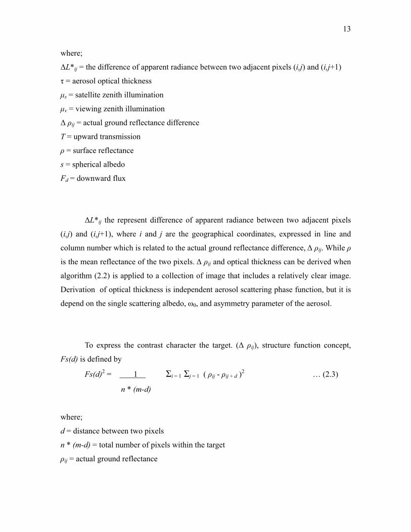
where;
∆L*ij = the difference of apparent radiance between two adjacent pixels (i,j) and (i,j+1)
τ = aerosol optical thickness
µs = satellite zenith illumination
µv = viewing zenith illumination
∆ ρij = actual ground reflectance difference
T = upward transmission
ρ = surface reflectance
s = spherical albedo
Fd = downward flux
∆L*ij the represent difference of apparent radiance between two adjacent pixels
(i,j) and (i,j+1), where i and j are the geographical coordinates, expressed in line and
column number which is related to the actual ground reflectance difference, ∆ ρij. While ρ
is the mean reflectance of the two pixels. ∆ ρij and optical thickness can be derived when
algorithm (2.2) is applied to a collection of image that includes a relatively clear image.
Derivation of optical thickness is independent aerosol scattering phase function, but it is
depend on the single scattering albedo, ω0, and asymmetry parameter of the aerosol.
To express the contrast character the target. (∆ ρij), structure function concept,
Fs(d) is defined by
Fs(d)2 = 1 Σi = 1 Σj = 1 ( ρij - ρij + d )2 … (2.3)
n * (m-d)
where;
d = distance between two pixels
n * (m-d) = total number of pixels within the target
ρij = actual ground reflectance

14
d is the distance between two pixels and n * (m-d) is the total number of pixels
within the target in composing structure function F*s(d). The structure function in
satellite observation is F*s(d) and the actual structure of the surface Fs(d) are related by
F*s(d) ≈ Fs(d) T (τa, µv) Fd (τa, µs) … (2.4)
1 – A * s(τa)
where;
A = mean albedo of the target
As provided that Fs(d) is known and invariant, the satellite measurements allow
us to estimate the aerosol optical thickness by means of the transmissions functions of
(2.4).
2.5 Derivation of Aerosol
Initially, distribution of aerosol always been monitored from ground-based
station. Many programmes have been developed in local and global scale. These
programmes provide aerosol monitoring services a well as validate the satellite
measurements.
Aerosol measurements began at the Climate Monitoring and Diagnostic
Laboratory (CMDL) baseline observatory in the mid-1970's apart of the Geophysical
Monitoring for Climate Change (GMCC) program. Since the inception of the program,
scientific understanding on the behavior of atmospheric aerosols has improved
considerably. One lesson has learned is that human activities primarily moreinfluence

15
aerosols in regional and continental scales rather than global scales. The goals of
regional-scale monitoring program are to characterize means, variability, and trends of
climate-forcing properties in different types of aerosols, and to understand the factors that
control these properties. CMDL's measurements also provide ground-truth observation
for satellite measurements and global models, as well as dominant aerosol parameters for
global-scale models. CMDL has various ground control station distribute across the
European region.
The Aerosol Robotic Network (AERONET) program is an inclusive federation of
ground-based remote sensing aerosol networks established by multi agency that are
related to aerosol studies. This program is distributed at hundred of stations around the
world purposely for monitoring global aerosol behaviour as shown in Figure 2.2. Their
goals are to assess aerosol optical properties and validate the network imposes standard
on instrument installation, sensor calibration and data processing. In this collaboration,
data of spectral aerosol optical depth and perceptible water and collected globally in
diverse aerosol regimes.
Figure 2.2: Distribution of AERONET station.

16
2.6 Aerosol Retrieval Using Remote Sensing
Decoupling the atmospheric effects such as water vapour, ozone absorption,
aerosol and molecular scattering from the terrestrial surface signal have been fairly
andsuccessfully achieved (Tanre et al., 1992). Unlike all, aerosols can be distinguished
accurately from ancillary data sources and used for satellite correction. This has led to the
development of aerosol retrieval in which the radiance from over ocean is inverted to an
appropriate aerosol model for obtaining the correct aerosol optical thickness at such
surface reflectance.
Aerosol remote sensing was developed using a single wavelength and single angle
of observation (Kaufman et al., 2002). TOMS (Total Ozone Mapping Spectrometer) has
flown since 1978, and it two channels that are sensitive to ultraviolet light that were
discovered to be excellent for observation of elevated smoke or dust layers above
scattering atmosphere observation. TOMS is among the first instrument to allow
observation of aerosols as the particles always spread across the land and sea boundary.
From TOMS data as in Figure 2.3, it is possible to observe a wide range of phenomena
such as desert dust storms, forest fires and biomass burning.

17
Figure 2.3: Aerosol condition from Earth Probe TOMS on 8 February 2005.
One of the first instrument designed for aerosol measurements is POLDER
(Polarization and Directionality of the Earth’s Reflectances). It relies on spectral channels
in a range wider than human vision ability (0.44 - 0.86µm). The instrument comprises a
wide-angle camera that observes similar target on the earth at different angles and up to
zenith angle of 65o. POLDER also measures light polarization to detect fine aerosols over
land, taking advantage of the difference between the spectrally neutral polarized light
reflected from the earth’s surface and the spectrally decreasing polarized light reflected
by fine aerosols.

18
Virtually, all procedures for retrieving aerosols from satellite data over land areas
require a priori knowledge of the surface and require a change detection procedure
(Holben et al., 1992). Typically, these have been developed using high resolution Landsat
and SPOT data. A complimentary technique was developed using TM data (Figure 2.4)
which selects invariant targets and relates the change in contrast between the invariant
targets to the aerosol optical thickness on a reference day (Sifakis et al., 1988). In a more
simplified approach, in term of brightness method, the apparent changes in reflectance
above a pixel from one day to another is related to the difference in optical thickness
between the two days assuming the surface reflectance did not has changes.
Figure 2.4: Aerosol optical thickness derived from Landsat TM over
Athens using contrast reduction approach (source: Sifiakis et al., 2002)
Two instruments, MODIS (Moderate Resolution Imaging Spectroradiometer) and
MISR (Multi-angle Imaging Spectroradiometer) on the Terra satellite have measured
global aerosol concentrations and properties since 2000. MODIS measures aerosol
optical thickness over land with an estimated error of ± 0.05 to ± 0.20 (Kaufman et al.,

19
2002). In land application, MODIS uses the 2.1µm channel to observe surface cover
properties, estimate surface reflectance at visible wavelength and derive aerosol optical
thickness from the residual reflectance at the top of atmosphere.
The amount of light penetrating the top of atmosphere is affected by the angle
where the light was reflected by the surface or atmosphere. MISR took advantage of this
fact by detecting the reflected light at different viewing angles (nadir 70o in forward and
backward motion) along the satellite’s track in a narrow spectral range (0.44-0.86µm). It
is thus able to separate the aerosol signal from that of surface reflectance and then
determine the aerosol properties. A mixed approach using two viewing directions but in a
wider spectral range (0.55-1.65µm) is used by ATSR (Along Track Scanning Radiometer)
to derive the aerosol concentration and type.
Over bright desert, the magnitude of dust absorption is determined if dust has
brightens or darkens the image. This property is very useful to estimate the aerosol
optical thickness. Such satellite measurements, in agreement with in situ, aircraft and
radiation network measurement of dust absorption, helped to solve a long standing
uncertainty in desert dust absorption of sunlight.
Advanced Very High Resolution Radiometer (AVHRR) instrument has been used
by numerous researches to detect aerosol optical thickness over land and oceans (e.g.,
Stowe et. al., 1997, Husar et. al., 1997, Hindman et. al., 1984, Paronis and Sifakis, 2003).
Unlike the nearest satellite sensors, AVHRR enables to provide a temporal coverage
which is not accessible since the past twenty years.
Atmospheric effect in NOAA depends on the position of spectral bands and
instantaneous field of view (IFOV) of the instrument. Sifakis et al. (2003) has studied the

20
potentiality of using NOAA-15 observations for obtaining AOT maps over the
metropolitan area of Athens through Differential Textural Analysis (DTA) algorithm. The
result from this study is presented in Figure 2.5. Correlation as high as 0.78 to 0.95 are
retrieved between the AOT values and PM10 measurements.
Figure 2.5: AOT distribution over Athens from NOAA imagery contrast
reduction technique (Sifakis et al., 2002)
CHAPTER 3
METHODOLOGY
3.1 Introduction
In this chapter will discuss about the methodology involved in this study. The
methodology is divided into three major parts: data acquisition, data pre-processing
and data processing. In this study, a pair of NOAA AVHRR (National Oceanic and
Atmospheric Administrator Advanced Very High Resolution Radiometer) imagery
were represent as fine day data and pollution occurrence data, PM10 (particulate
matter smaller than 10µm) also used in the processing. In preprocessing radiometric
correction, geometric correction and water masking routine were implemented
initially on both satellite images
Contrast reduction technique is used in order to extract the aerosol optical
thickness (AOT). Contrast reduction technique is divided into two major processing
schemes. Differential Textural algorithm is applied to the calibrated channel 1 NOAA
data. After that, Thermal Band Difference is applied to thermal channel in order to
allow a cross-checking on the results from contrast reduction procedure. Figure 3.1
shows the workflow of the study.

21
Figure 3.1: Research operational framework.
Data
acquisition D
ata Pre-processing
Data
Processing A
nalysis R
esult PM10 data Reference
image
Radiometric Correction
Geometric Correction
Water Masking
Pollution image
Map of Aerosol composition
Differential Textural Analysis algorithm
Thermal Band Difference algorithm
Correlation with in situ data

22
3.2 Data Collection
A series of NOAA 16 data are used in this study. Each series is composed by:
i. A ‘reference image’, which is ideally, represented as pollution-free image, and.
ii. A ‘pollution image’, which corresponds to a representative or characteristic
pollution level.
Data selection is necessary for the reliability of results. Images are selected
according to the availability of pollution measurement by a maximum number of
monitoring stations and representativeness of the pollution levels recorded by local
monitoring networks, or by the standard criteria for image quality and cloud cover.
Table 3.1 tabulated the date of three images used as Reference Image in this study.
The data are taken from three different dates in years from 2002 to 2004.
Table 3.1: List of data used as Reference Image.
Reference Data Date
1 Reference 1 17/05/2002
2 Reference 2 18/06/2003
3 Reference 3 18/05/2004
The data represented polluted day are listed in table 3.2. Both of the reference and
polluted data were taken at 3.00 p.m. in local time. These data set are considered
suitable for this study by assuming that the atmosphere is stable to active industrial
event at data acquisition time.
Table 3.2: List of data used as Polluted Image
Polluted Data Date
1 Polluted 1 20/07/2002
2 Polluted 2 08/06/2003
3 Polluted 3 26/05/2004

23
Accuracy assessment is carried out by taking a collection of in situ data into
the processing. In situ data as PM10 ground based measurement provided by Alam
Sekitar Malaysia Berhad (ASMA). These data were collected at 5 monitoring stations
evenly distributed over Peninsular Malaysia namely, Kuala Lumpur (101° 42.274' E,
03° 08.286' N), Prai (100° 24.194’ E, 05° 23.890’ N), Pasir Gudang (103° 53.637' E, 01°
28.225' N), Bukit Rambai (102° 10.554' E, 02° 15.924' N) and Bukit Kuang (103° 25.826'
E, 03° 16.260' N).
3.3 Pre-processing
In data pre-processing, three major process namely geometric correction,
radiometric correction and masking of water area were applied to the image before
further processing is carried out.
3.3.1 Geometric Correction
Firstly, pre-processing started at which the processing concerns the
geometrical control on both images. It is proposed to super-impose the images
to a topographic map. The images are rectified relatively according to a map
projection by with the least-square regression method and resampled relative
pixel by the nearest-neighbour algorithm in order to maintain distribution
patterns of the pixels and avoid any error on the raw radiometric values.
Corrected images were projected to Geographic Lat/Long Projection with
Everest (Malaysia and Singapore, 1948) Datum. The reference points used to
resample the satellite images were taken from vector layer representing
Malaysia boundary. The RMS error for each images are shown in Table 3.3.
Generally, the RMS error is lower and considered accurate enough to be used in

24
further processing. At least 12 to 20 points were used to correct each images in
its proper geometry.
Table 3.3: RMS error value for each image.
Images Control point error in x
(pixel)
Control point error in y
(pixel)
Total RMS error (pixel)
Reference 1 0.0200 0.0669 0.0698
Reference 2 0.0262 0.0082 0.0275
Reference 3 0.0293 0.0386 0.0484
Polluted 1 0.0170 0.0091 0.0193
Polluted 2 0.0696 0.0271 0.0747
Polluted 3 0.0640 0.1044 0.1224
The effect of geometry correction process is shown in figure 3.2(a) and (b). The
corrected imageis shown in figure 3.2 (b) and it has the same coordinate in the real
world.
(a) (b)
Figure (3.2): (a) Original NOAA-16 datataken on 18 May 2004 in Channel 1, 2 and 4.
(b) Geometrically corrected image.

25
3.3.2 Radiometric Correction
Radiometric correction is applied by transforming the values of digital number
(DN) to radiance or reflectance values through the algorithm as follows:
A = S + I … (3.1)
where;
A = Reflectance factor or scale of radiance (albedo)
S = Slope value
I = Intercept value
The result of radiometrically corrected process is shown in figure 3.3.
(a) (b)
Figure 3.3: (a) Geometrically corrected image. (b) Calibrated image.
3.3.3 Masking Out Water Bodies
Masking image is an image with two representating the land area and water
surface. In order to extract aerosol information over land area, all the information

26
related to sea surface and water bodies must be isolated and excluded out from the
calibrated images, as in figure 3.4 (a). This study area is consisted of 328 550 km2 of
land area and 1 200 km2 of water area. Water bodies were found along South China
Sea and Straits of Malacca as well as within lake, river and other water bodies as
shown in figure 3.4 (b). This process is applied to each image used in the study.
(a) (b)
Figure 3.4: (a) Calibrated NOAA data. (b) Masked of water images.
3.4 Satellite Data Processing
After pre-processing procedure, further processing is applied in order to extract
aerosol optical thickness distribution over land area. The processing, namely contrast
reduction maps the AOT by comparing the fine day data with polluted day data.
Contrast reduction is carried out by performing Differential Textural Analysis (DTA)
and temperature attenuation procedure on channel 1and 4 calibrated of NOAA data,
respectively.

27
3.4.1 Differential Textural Analysis (DTA)
Differential Textural Analysis (DTA) uses two images namely a ‘Reference’
and a ‘Polluted’ image that have been acquired on a low pollution and a high pollution
day. The underlying surface between the two acquisition images must be relatively
unchanged and taken in same observation geometry. Hence, it has minimized the
uncertainties due to both the seasonal variations of the ground reflectance and the
surface bi-directionality effect (Paronis and Sifakis, 2003).
The main part of DTA calculates the local standard deviation of radiance in
both images as follows:
σ = Σ ( ρ – µ )2 … (3.2) n
Where;
σ = Local standard deviation of radiance values
ρ = Radiance of Channel 1
µ = Local mean of radiance values
n = pixels of 3x3 local window
Sifakis et al (2003) used 7 x 7 pixels window to measure out the standard
deviation due to availability of huge number of ground-based data. Therefore, it is
sufficient enough to used 3 x 3 pixels window in small number of ground-based data.
The result presented in figure 3.5.

28
Figure 3.5 : Local standard deviation image from 3x3 windows .
The presence aerosol layer in the atmosphere has reducing effect in image
contrast. The contrast reduction is directly related to the optical thickness of the layer
(Tanre et al. , 1993). The ratio of contrast between two different day images on two
different days is expressed as:
τ = ln σ ( ρ reference ) … (3.3)
σ ( ρ pollution )
where;
τ = optical thickness values
σ = Local standard deviation of radiance values
ρ reference = radiance values of Channel 1of reference image
ρ pollution = radiance values of Channel 1of pollution image

29
Figure 3.6: Structure of DTA model.
In order to cross-checking on the result, temperature attenuation procedure is
applied to the reference and pollution image by maintaining only land areas from
calibration of thermal band. Thermal band values are converted to radiance by
formula of:

30
NE = a0 + a1CE + a2CE2 … (3.4)
where;
NE = radiance value in mW/(m2-sr -cm-1)
a0, a1, a2 = thermal operational coefficient of channel 4
CE = DN value of channel 4
To convert radiance value into an equivalent blackbody temperature, two
processing steps as follows have to be defined
TE* = C2Vc . (3.5)
C1Vc3
NE
TE = TE* - A … (3.6) B
where;
TE = Equivalent blackbody temperature
C1 = 1.1910427 x 10⁻⁵ mW/(m2 -sr-cm-4 )
C2 = 1.4387752 cm-K
Vc = 917.2289 (for NOAA-16)
A = 0.332380 (for NOAA-16)
B = 0.998522 (for NOAA-16)
Temperature attenuation is applied to estimate the observed relative
temperature variation with the result shown in Figure (3.7). TBDF or thermal band
difference are carried out through the following algorithm
TBDF = ( TE reference ) – ( TE pollution ) … (3.7)
where;
TE reference = Equivalent blackbody temperature for reference image
TE pollution = Equivalent blackbody temperature for polluted image
ln 1 +

31
Figure 3.7: Thermal band difference image of Reference 3 and Polluted 3 images.
Finally, information related to water bodies are excluded from the result cross-
checking the DTA images and TBDF images. DTA images that have TBDF value
lower than 1 are replaced by 0.

CHAPTER IV
RESULT AND ANALYSIS
4.1 Introduction
This chapter discussed and analyzed the output obtained through this study. The
discussions are divided into final map analysis and regression analysis from
correlation graph.
4.2 Aerosol Optical Thickness (AOT) Distribution From NOAA-16
Figure 4.1 shows the distribution of aerosol optical thickness (AOT) over land
of Malaysia on 20/07/2002. It is shown clearly by the figure that the AOT value over
Malaysia are low. It should be noted that ‘Unclassified’ pixels over the northern part
of Peninsular Malaysia were due to the presence of cloud appearing in Reference 1
image. This situation is consequent to cloud presence in the reference images,
indicating the importance of choosing the appropriate cloud-free reference images.
Aerosols concentration are indicated through the colour of red for high AOT value
and blue for low AOT value.

34
Figure 4.1: AOT maps derived from ‘Reference’ and ‘Polluted’ images of 17/05/2002
and 20/07/2002, respectively
Pixels distribution is shown in Figure 4.2. The pie chart show that 75% of the
pixels in the image are represent ‘Unclassified’ pixels. This is due to the presence a lot
of cloud especially in the Reference 1 image. The cloud can be identified in almost
half of Peninsular Malaysia area. The ‘Unclassified’ pixel also represent water body
area whish is cover almost 60% of the study area. The highest concentration of AOT
indicated by red colour represent 1573 pixels from the whole image. This red pixel
can be found in Pulau Borneo and Johor Bahru. While the lowest AOT values indicate
by dark blue in colour is represent 11% of the pixels from the image.
Figure 4.2: Partition of AOT value on 20/07/2002.

35
Figure 4.3 shows the distribution of aerosol optical thickness (AOT) over land
of Malaysia derived on 18/06/2003. Aerosols concentration are indicated through
temperature aggregation which the colour of red for high AOT value while blue for
low AOT value. It is shown clearly by the figure that the AOT value over Malaysia
are low. High AOT value can be found in Pulau Pinang, along West Peninsular
Malaysia, Johor Bahru, Singapore and some places in Sarawak. Most of this places
are industrial and high population area.
Figure 4.3: AOT maps derived from ‘Reference’ and ‘Polluted’ images of 08/06/2003
and 18/06/2003, respectively.
Figure (4.4), show a pie chart with the percent distribution of AOT pixels. The
aerosol distribution over Malaysia on 18/06/2003 are higher compare to Figure (4.1).
1% of the region gain a high aerosol measurement which is represent 11368 pixels
from total of 2226560 pixels per image.

36
The DTA algorithm applied on a series of AVHRR data over Malaysia region.
From the study, aerosol distribution over Malaysia on 26/05/2004 (as shown in Figure
4.5) is relatively low. Only Penang shows a high value of AOT. Some places with high
population, namely Kuala Lumpur and Johor Bahru also gain high aerosol
concentration.
High AOT values (depicted in red) over sea area were due to the presence of
clouds appearing and has to be ignored because the algorithm used in this study is
only valid for extraction of AOT value over land and not effective for water surface.
Figure 4.4: Partition of AOT distribution derived on 08/06/2003.

37
Figure 4.5: AOT maps derived from ‘Reference’ and ‘Polluted’ images of
18/05/2004 and 26/05/2004, respectively.
AOT distribution derived from 26/05/2004 is shown in Figure 4.6. The pie
chart show that 83% of the pixels in the image are represent ‘Unclassified’ pixels.
‘Unclassified’ pixels are covered cloud and water area. The highest concentration of
AOT indicated by red colour represent 2535 pixels from the whole image.
Figure 4.6: Partition of AOT distribution derived on 26/05/2004.

38
4.3 Correlation of AOT With PM10
The accuracy of the results was correlated against PM10 ground based
measurements provided by Alam Sekitar Malaysia Berhad (ASMA). PM10 is referred
to particulate matter that has a size less than 10 microns. These data were collected at
5 monitoring stations evenly distributed in Malaysia namely, Kuala Lumpur, Prai,
Pasir Gudang, Bukit Rambai and Bukit Kuang. The respective scatter plots are
presented in Figure 4.7, Figure 4.8 and Figure 4.9.
Figure 4.7: Retrieved AOT distribution vs PM10 value for 20/07/2004.
All the data reveal a good relationship with PM10 measurements where the r2 is
exceeding 0.8. It is noteworthy that the correlation coefficients are high for 2002,
2003 and 2004 (0.9567, 0.8633 and 0.8361, respectively). From the study, Bukit
Kuang recorded the lowest aerosol distribution both from the PM10 measurement and
AOT retrieval from satellite. This is maybe because it is located in non-urban area.
Kuala Lumpur and Pasir Gudang used to gain the highest aerosol measurement.
AOT Distribution of 20/07/2002
R2 = 0.9567
0100200300400500600700800
0 20 40 60 80 100
PM10 (µgr/m3)
AO
T (*
1000
)

39
AOT Distribution of 18/06/2003
R2 = 0.8633
0
100
200
300
400
500
600
700
800
0 20 40 60 80 100 120
PM10 (µgr/m3)
AO
T (*
1000
)
Figure 4.8: Retrieved AOT distribution vs PM10 value for 18/06/2003.
This agreement suggests that the application of the DTA algorithm on NOAA-
16 AVHRR images whenever available and cloud free could be used to provide daily
AOT maps, depicting air quality information for Malaysia region.
AOT Distribution of 26/05/2004
R2 = 0.8361
0100200300400500600700800
0 10 20 30 40 50
PM10 (µgr/m3 )
AO
T (*
1000
)
Figure 4.9: Retrieved AOT distribution vs PM10 value for 26/05/2004.

CHAPTER V
CONCLUSION
5.1 Conclusion
This research presented the potential of extracting AOT map from low
resolution data, NOAA-16 over Malaysia region. The high correlation is found
between AOT values and PM10 measurement, which suggest that the application of
DTA algorithm is best used on available and cloud free AVHRR imagery. In fact, the
daily AOT maps indicate air quality information which are somehow minimizing the
cost and time compared to the conservative observation.
However, the method is usually restricted due to its low spatial resolution.
This could be possibly alleviated by the synergistic ue of high spatial resolution
images (i.e Landsat TM and SPOT XS. Cloud presence also could be one of the great
limitation for the result reliability a tropical area as Malaysia. Cloud cover is a major
problem and in thus limit the accuracy of the results.limitation is a very common
problem.

41
5.2 Recommendation
The dynamic movement of aerosol over land and oceans requires frequent
monitoring from the space. In fact the dynamic range and out sources of aerosols are
mostly generated from the land. Likely, the remote sensing of aerosol is particularly
important to digest human understanding on transformation of aerosol in atmosphere
on transformations of aerosol in atmosphere. In comparison, aerosol above the ocean
regions is more accurate to be retrieved and much informative due to dark `
and uniform ocean reflectance. Ocean occupies 2/3 of the earth surfaces and naturally
interacts with 2/3 of the solar radiation. By relying with remote sensing in routine
observation, the behavior of aerosol in the atmosphere could be exposed and
consequently, initial prediction of corresponding human activity involved in the
aerosol formation will be determine.
The addition of active sensors such as lidar, makes it possible to measure thin
aerosol layers which are not easily observed by multispectral scanners. The well
calibrated radiometers in conjunction with lidar measurement which observed at the
same accuracy of tropospheric aerosol level, particularly in low optical thickness
conditions.
Remote observation from space has discovered aerosol in term of its physical
and optical properties. The combination spaceborne with ground based measurement
permits the observation comprehensive description of aerosol impact on the earth
climate. Finally, both measurements are useful to derive the solid aerosol optical
properties over the world.

REFRENCES
Andreae, M. O.,Browell, E. V., Garstang, M., Gregory, G. L., Harris,R. C., Hill, G. F.,
Jaqcob, D. J.,Pereira, M. C., Sachse, G. W., Setzer, A. W., Silva Dias, P. L.,
Tablot, R. W., Torres, A. L, and Wofsky, S. C., (1988). Biomass burning
emissions and associated haze layers over Amazonia. Journal Geophysical
Research, 93, 1509-1527.
Charlson, R. J., Schwartz, S. E., Hales, J. M., Cess, R. D., Coakley, J. A., Hansen, J.
E., and Hoffman, D. J. (1992). Climate Forcing By Anthropogenic Aerosols.
Science, 255, 423-430.
Cofala, J., Amann, M., Gyarfas, F., Schoepp, W., Boudri, J. C., Hordijk. L., Kroeze,
C., Junfeng, L., Dai Lin, Panwar, T. S. and Gupta, S. (2004). Cost-effective
Control of SO2 Emission in Asia. Journal of Environmental Mangement 72, 149-
161.
Crutzen, P. J., Delany, A. C., Greenberg, J., Haagenson, P., Heidt, L., Leub, R.
Pollock, W., Seiler, W., Wartburg, A. and Zimmerman, P. (1985). Tropospheric
chemical composition measurements in Brazil during the dry season. Journal
Atmospheric Chemistry, 2, 233-256.
Griggs, M. (1975). Measurements of the atmospheric aerosol optical thickness over
water using ERTS-1 data. J. Air Pollution Control Assessment, Vol. 25, 622-626.
Hansen, J. E. and Lacis, A. A. (1990). Sun and Dust Versus Greenhouse Gaseous: An
Assessment of Their Relative Roles in Global Climate Change. Nature, 346,
713-719.
43
Holben, B. N., Eric Vermote, Kaufman, Y. J., Tanre, D., and Kalb, V. (1992). Aerosol
Retrieval over Land from AVHRR Data-Application for Atmospheric
Correction. IEEE Transaction on Geoscience and Remote Sensing, Vol. 30, No.
2, 212-221.
Isakov, V. Y., Feind, R. E., Vasilyev, O. B. and Welch, R. M. (1996). Retrieval of
Aerosol Spectral Optical Thickness from AVIRIS Data. IEEE.
Kaufman, Y. J., Tanre, D., Boucher, O. (2002). A Satellite View of Aerosols in the
Climate System. Nature, Vol. 419, 215-223.
Lacis, A. A. and Mishchenko, M. I. (1995). Climate forcing, climate sensitivity, and
climate response: A Radiative Modeling Perspective on Atmospheric Aerosols.
Aerosol Forcing Climate. Pp 11-42, John Wiley, New York.
Ortiz, V., Figueroa, M., Picon, A. (2003). Aerosol and Cloud Properties Retrieval
Using MODIS and MISR. NOAA-CREST/NASA-EPSCoR Joint Symposium
for Climate Studies.
Paronis, D. and Sifakis N. (2003). Satellite Aerosol Optical Thickness Retrieval Over
Land With Contrast Reduction Analysis Using A Variable Window Size. IEEE
Penner, J. E., Dickinson, R. E., and O’Neill, C. A., (1992). Effects of aerosol from
biomass burning on the global radiation budget. Science, 256, 1432-1433.
Reid, J. P. and Sayer, R. M. (2002). Chemistry In The Clouds: The Role of Aerosols In
Atmospheric Chemistry. Science Progress(2002), 85(3), 263-296.
Sifakis, N., Soulakellis, N. Gkoufa, A. (1988). Manual of EO Image Processing
Codes.
Sifakis, N., Soulakellis, N., Paronis, D. and Mavrantza, R. (2002). Manual of EO
Image Processing Codes, Revised Reference Manual V.1.1.

44
Tanre, D., Deschamps, P. Y., Devaus, C. and Herman, M. (1993). Estimation of the
Saharan Aerosol Optical Depth From Blurring Effects in Thematic Mapper Data.
Journal of Geophysical Research, 15955-15964.
Tanre, D., Holben, B. N., Kaufman, Y. J. (1992). Atmospheric Correction Algorithm
for NOAA-AVHRR Products: Theory and Application. IEEE Transaction on
Geoscience and Remote Sensing, Vol. 30, No. 2, 231-248.