AN ANALYSIS OF FINANCIAL MANAGEMENT

STRATEGIES FOR NEW GENERATION COOPERATIVES

UNDER CONDITIONS OF RISK

A Thesis Submitted to the Graduate Faculty

of the North Dakota State University

of Agriculture and Applied Science

By

Bradley James Streifel

In Partial Fulfillment of the Requirements for the Degree of

MASTER OF SCIENCE

Major Department: Agribusiness and Applied Economics

March 2002

Fargo, North Dakota

ii

This page is to get the page numbers correctly aligned

iii

ABSTRACT

Streifel, Bradley James, M.S., Department of Agribusiness and Applied Economics, College of Agriculture, North Dakota State University, March 2002. An Analysis of Financial Management Strategies for New Generation Cooperatives Under Conditions of Risk. Major Professor Dr. William Nganje. The objective of this study is to analyze the effects of different income

allocation strategies on New Generation Cooperatives (NGC’s) given different levels of

risk inherent in their industries. A stochastic simulation model is used to capture the

input and output price risk along with the uncertainty in demand.

A utility maximization framework is employed to find the solvency (equity to

asset) level that maximizes the NGC’s membership utility as a function of expected

return on equity, variance of return on equity, and member’s risk aversion. Next, the

effects that changes in business and financial risk have on the optimal solvency ratios

are examined. Then, allocation strategies are introduced to the model as a way to

adjust their solvency levels to maximize the member’s utility.

The results of this study show that each NGC will have unique optimal solvency

levels. For example, at a risk aversion of 6, Dakota Growers has an optimal solvency

level of 61%; American Crystal has an optimal solvency of 18%; Min Dak has an

optimal solvency of 46%; and NGC Bean Cooperative has an optimal solvency of 58%.

While each of the NGCs displayed large differences in their optimal solvency, they all

displayed similar reaction to changes in return on assets, variability of return on assets,

interest rates, and variability of interest rates. The NGCs were also found to have

similar reactions to changes in allocations strategies, but effectiveness of these changes

was different across NGCs.

iv

ACKNOWLEDGMENTS

I would like to thank my adviser, Dr. William Nganje, for his guidance and

motivation. I appreciate the committee members, Dr. Cheryl DeVuyst, Dr. William

Nelson, and Dr. Matthew Walker, for their constructive suggestions and comments.

I would also like to thank Mr. Frayne Olson and Mr. Edward Janzen for their

valuable contribution with the deterministic model and for their efforts throughout the

completion on this study.

I really appreciate my precious family and friends for their love and

encouragement. Special appreciation goes to my wife, Renae, for all her hours

proofreading and patience on many long nights of work.

v

TABLE OF CONTENTS

ABSTRACT…………………………………………………………………….. iii

ACKNOWLEDGMENTS………………………………………………………. iv

LIST OF TABLES………………………………………………………………. vii

LIST OF FIGURES……………………………………………………………... viii

CHAPTER I. INTRODUCTION…………………………………….…………. 1

Description of the Problem…...…………………………………………. 1

Current Allocation Strategies…………………………………………….. 3

History of NGCs……………………………………………………….. 5

Importance of NGCs……………………………………………………. 8

Contribution of the Study……………………………………………….. 10

Objectives of the Study…………………………………………………. 10

Methodology……………………………………………………………. 11

Organization of the Thesis……………………………………………….. 12

CHAPTER II. LITERATURE REVIEW………………………………………… 13

Risk Identification and Measurement…………………………………… 13

Optimal Solvency Studies………………………………………………. 18

Dividend Policy as an Effective Financial Management Strategy for NGCs…….…………………………………... 19

Unique Characteristics and Tax Implications of NGCs….……………… 23

CHAPTER III. METHODOLOGY AND DATA………………………………… 36

Theoretical Model……………..…………………………………………. 36

Optimal Solvency and Allocation Decision Model………………………. 40

CHAPTER IV. DATA AND RESULTS……………………….………………… 48

vi

Data Sources….……….…………………………………………………. 48

Results………………………………………………….………………… 56

CHAPTER V. SUMMARY AND CONCLUSIONS…………..………………… 67

Purpose of the Study…………………………………..………………… 67

Objectives of the Study…………………………………………...……… 67

Methods Used in the Study……………………………………………….. 68

Results and Conclusions.…………………………….…………………… 69

Implications for Management……………………………………………. 79

Suggestions for Further Research………………………………………... 80

REFERENCES…………………………………………………………………... 82

APPENDIX A. PERCENT OF ALL EQUITIES MODEL………………………. 86

APPENDIX B. OPTIMAL SOLVENCY CALCULATOR.…………………….. 89

APPENDIX C. DESCRIPTION OF NET INCOME BEFORE TAX AND DEBT…………………………….……………………….. 90

vii

LIST OF TABLES

Table Page

1.1 Industries Where NGCs are Present………….……………………………... 7 2.1 Business Risk Comparison of Dakota Growers Pasta and

American Crystal Sugar Cooperative………………………………………. 14 4.1 Summary Statistics by Year for Each NGC (in Thousands)..……………… 55 4.2 Empirically Determined Solvency Ratios and Sensitivity

Analysis of Each NGC ……………………………………………………... 57 4.3 Probability of Negative Rate of Return on Equity for Each NGC…………... 60 4.4 Effects of Allocation Strategies on Solvency and the Probability

of a Negative Rate of Return on Equity for Each NGC……………………... 62 4.5 Effects of Revolvment Cycle Length Changes on the Solvency and

Probability of Equity Loss for NGC Bean Cooperative……………………. 63 4.6 Value at Risk Extension for NGCs at Different Risk Aversion

Coefficients………………………………………………………………… 65 4.7 Value at Risk Extensions for NGCs at Different Income Allocation

Percentages…………………………………………………….…………… 66 B.1 Calculation of Optimal Solvency…………………………………………… 89

viii

LIST OF FIGURES

Figure Page

1.1 The Percentage of Net Income Retained for Dakota Growers Pasta, American Crystal Sugar, and Minn-Dak Sugar……………………. 4 1.2 Trend in the Number of Farmer Marketing Cooperatives from

1962-1996………………………………………………………….. …….. 9 5.1 Behavior of Optimal Solvency Levels for NGCs when the Risk

Aversion Coefficient is Varied from One to Ten…………………………. 70 5.2 Behavior of Return of Equity for NGCs when the Risk Aversion

Coefficient is Varied from One to Ten…………………………………… 70 5.3 The Changes in the Standard Deviation of ROE for NGCs as the

Risk Aversion Coefficient is Varied from One to Ten………………….... 72 5.4 The Probability of a Negative ROE at Different Risk Aversion Coefficients.……………………………………..……………... 73 5.5. Solvency Positions of the NGCs when the Income Retained

is Varied from 0 Percent to 100 Percent…………………….……….…….. 74 5.6 The Probability of Equity Loss for NGCs at Different

Allocation Percentages……………………………………………………. 75 5.7 Solvency Level of NGC Bean Cooperative at Different Income

Allocation Percentages when the Revolvment of Retained Income is Varied from One to Ten Years…...……………………………………... 76

5.8 Value at Risk of the NGCs when the Risk Aversion Coefficient

is Varied from One to Ten……………………...…………………..…….. 78 5.9 The Change in the Value at Risk for the NGCs when the Income

Retained is Varied from 0 Percent to 100 Percent for NGC's at Different Allocation Strategies………………………………………..….. 78

1

CHAPTER I

INTRODUCTION

Description of the Problem

In the 1970s New Generation Cooperatives (NGCs) broke new ground with their

financial and business structure. Stefanson and Fulton (1997) stated that the primary

reason for newly forming cooperatives to employ the NGC structure is the necessity to

have substantial equity capital before debt funding will be made available. NGCs are able

to fill this need because their closed-contract structuring allows for participation in the

business based directly on the members’ investment in membership stock. By doing so, the

NGC structure ties the ability to benefit from patronizing the cooperative to the amount

members invest. Thus, the NGC structure has made it easier for cooperatives to sell large

amounts of shares and raise large sums of money for up front investment.

A second reason that NGC structuring is being used is that members of traditional

cooperatives have been dissatisfied with the low percentages of cash allocations and long

revolving times for the payment of the remainder of their dividends. This dissatisfaction of

cooperative members has motivated the developers of new cooperatives to apply radically

different financial management strategies to their businesses. For example, many NGCs

have returned a large percentage of their profits to the members/investors in the year

earned. Then, they will return to the membership using equity drives for additional

investments when more capital is needed for a planned expansion. Also, many NGCs have

maintained a goal to revolve the retained portion of the dividends in a relatively short time-

2

frame of five to ten years. This strategy is quite radical in comparison to the traditional

cooperatives that have established retention periods of much longer, often until retirement.

These financial management strategies are still in formation due to the relatively short

history of NGCs. Therefore, the full implications of these financial strategies are not

known at this time as many of the NGCs are learning as they go.

For the NGCs, the decision on how to allocate net income has both short-term

(current year) as well as long-term (five to twenty years) ramifications on membership

satisfaction. Since the members have made a direct equity investment, there is an

expectation that the NGC will return a significant portion of the net income in the form of

cash (rather than being retained by the cooperative as additional equity). In the short term,

cash dividends are beneficial for the membership and have a tendency to increase the value

of the limited NGC stock because stock value is derived mainly from current and future

dividend payment expectations. Increasing stock values also bring distinct advantages to

the NGC. For example, if new equity stock sales are planned for expansion, high stock

values will attract people to invest as they can see how well the investment has been for the

current membership.

Over the long term, returning a high percentage of the cooperative's net income in

cash may leave the cooperative in a vulnerable financial position where it is unable to

handle adverse fluctuations in income. In fact, inaccurate projections, adopting uniform

financial strategies, and ineffective planning have been cited as major reasons that about 40

percent of NGCs fail (Stefanson et al., 1995). In Minnesota and North Dakota, the

vulnerability of NGCs is quite apparent in the large number that have either failed or went

through a financial restructuring process. The failure of these NGCs has a devastating

3

impact on both their producer members, who have invested in these companies, and the

communities, that depend on the production facility for workforce employment and income

tax revenue. This study aims to increase the successfulness of NGCs by exploring

allocation strategies that incorporate risk and have the potential to lower the probability of

NGC failures.

Current Allocation Strategies

For many of the newly formed NGCs, adopting the appropriate strategies has

proven to be a difficult task. There has been a strong temptation for newer NGCs to look

to the more established businesses for models of income allocation and equity

management. This strategy can be very dangerous since each cooperative is unique. That

is, each NGC will face different industry conditions, competitive environments, strategic

goals, and risks. In addition, each NGC will have its own financial conditions.

Two examples of the vast differences between NGCs can be seen in the pricing

structures of American Crystal Sugar and Dakota Growers Pasta. American Crystal Sugar

and the other sugar cooperatives of the Red River Valley use a delayed pricing system

combined with a per-ton retain to build owner equity and to minimize debt capital. To

clarify, a per-ton retain is a reduction in the payment price of the commodity to the member

at the time of delivery. This payment reduction effectively lowers the cooperative’s cost of

raw materials, which leads to increased net income distributed to the members at a later

date. This system has worked well for the sugar beet growers who have no secondary

market for their product and, until recently, a fairly stable government supported price.

Dakota Growers Pasta, however, operates in a highly competitive market for both

4

processing inputs (durum) and finished product. It pays the current market price to the

growers and returns most of its profits in the form of a cash refund. This strategy has

provided members with a stable source of income along with a generally strong return on

their investment.

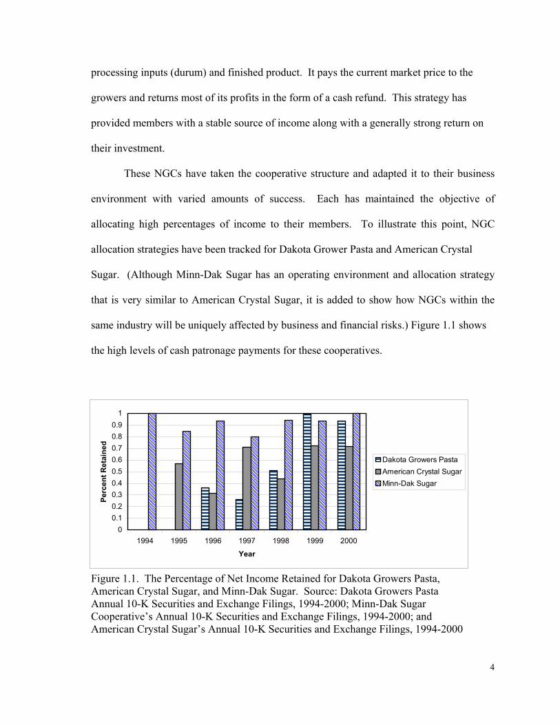
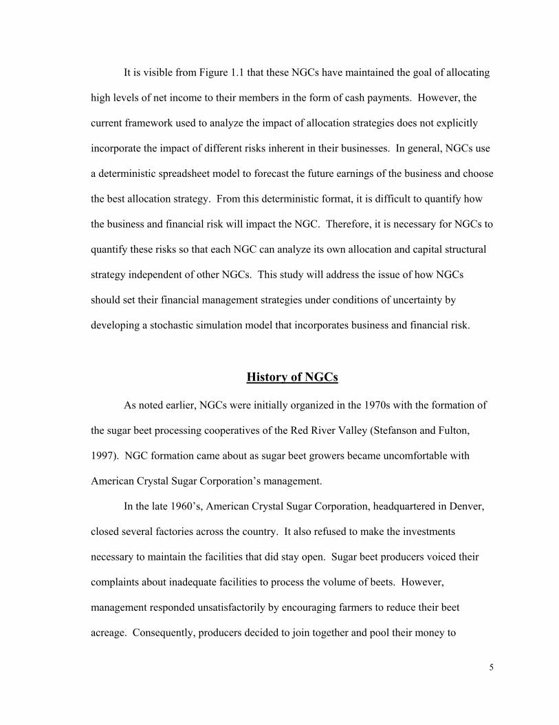
These NGCs have taken the cooperative structure and adapted it to their business

environment with varied amounts of success. Each has maintained the objective of

allocating high percentages of income to their members. To illustrate this point, NGC

allocation strategies have been tracked for Dakota Grower Pasta and American Crystal

Sugar. (Although Minn-Dak Sugar has an operating environment and allocation strategy

that is very similar to American Crystal Sugar, it is added to show how NGCs within the

same industry will be uniquely affected by business and financial risks.) Figure 1.1 shows

the high levels of cash patronage payments for these cooperatives.

Figure 1.1. The Percentage of Net Income Retained for Dakota Growers Pasta, American Crystal Sugar, and Minn-Dak Sugar. Source: Dakota Growers Pasta Annual 10-K Securities and Exchange Filings, 1994-2000; Minn-Dak Sugar Cooperative’s Annual 10-K Securities and Exchange Filings, 1994-2000; and American Crystal Sugar’s Annual 10-K Securities and Exchange Filings, 1994-2000

�������������������������

������������������������

�����������������������������������

������������������������������������������������������������

������������������������������������������������������������������

������������������������������������������������������������

������������������������������������������������������������

�������������������������������������������������������

��������������������������������������������������

������������������������������������������������������������������

�������������������������������������������������������

������������������������������������������������������������

00.10.20.30.40.50.60.70.80.9

1

1994 1995 1996 1997 1998 1999 2000

Year

Perc

ent R

etai

ned ����

����Dakota Growers PastaAmerican Crystal Sugar����

����Minn-Dak Sugar

5

It is visible from Figure 1.1 that these NGCs have maintained the goal of allocating

high levels of net income to their members in the form of cash payments. However, the

current framework used to analyze the impact of allocation strategies does not explicitly

incorporate the impact of different risks inherent in their businesses. In general, NGCs use

a deterministic spreadsheet model to forecast the future earnings of the business and choose

the best allocation strategy. From this deterministic format, it is difficult to quantify how

the business and financial risk will impact the NGC. Therefore, it is necessary for NGCs to

quantify these risks so that each NGC can analyze its own allocation and capital structural

strategy independent of other NGCs. This study will address the issue of how NGCs

should set their financial management strategies under conditions of uncertainty by

developing a stochastic simulation model that incorporates business and financial risk.

History of NGCs

As noted earlier, NGCs were initially organized in the 1970s with the formation of

the sugar beet processing cooperatives of the Red River Valley (Stefanson and Fulton,

1997). NGC formation came about as sugar beet growers became uncomfortable with

American Crystal Sugar Corporation’s management.

In the late 1960’s, American Crystal Sugar Corporation, headquartered in Denver,

closed several factories across the country. It also refused to make the investments

necessary to maintain the facilities that did stay open. Sugar beet producers voiced their

complaints about inadequate facilities to process the volume of beets. However,

management responded unsatisfactorily by encouraging farmers to reduce their beet

acreage. Consequently, producers decided to join together and pool their money to

6

purchase the sugar processing facility. In order to raise the $86 million for the purchase,

the group organized as a cooperative and issued a fixed amount of stock to be sold to the

growers (American Crystal Sugar Website, 2000). Ownership of this stock carried the

right and obligation to deliver beets grown over a specified acreage to the plant (Black et

al., 1999). By including the obligation to deliver, American Crystal laid the groundwork

for the first NGC.

Shortly after the formation of American Crystal Sugar, other sugar beet growers

recognized the benefits of this structure and replicated it across the Red River Valley

(Stefanson and Fulton, 1997). In 1999, the three sugar beet cooperatives (American

Crystal, Minn-Dak, and Southern Minn) included about 2,000 members and produced over

30 percent of the sugar grown in the United States (Black et al.,1999).

The success of the sugar beet cooperatives provided encouragement for farmers and

ranchers who seek to add value to the primary products they once sold as raw materials

(Stefanson and Fulton, 1997). This success has led to the proliferation of a wide variety of

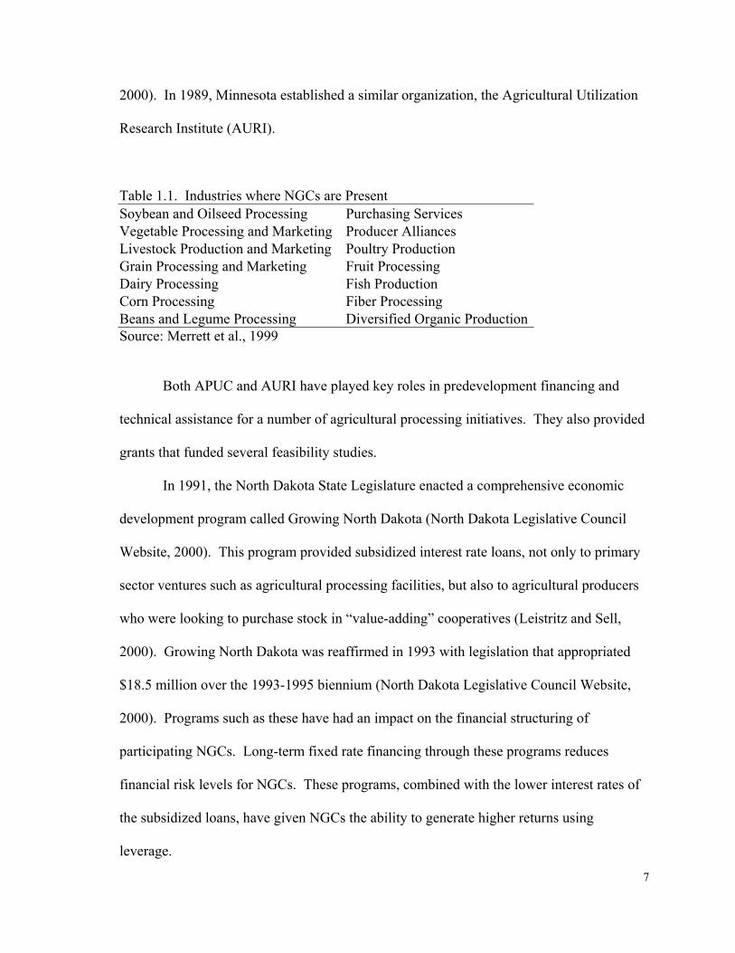
NGCs around the region. Table 1.1 (following page) shows that NGCs are present in 14

agricultural sectors.

It is apparent that the NGC structure has been adapted to several different industries

around the country. This diversity adds to the importance of developing income allocation

and capital structuring plans that are tailored to individual businesses with differing risks.

Most of the ventures listed in Table 1.1 started within a short time frame in the

1990s taking advantage of recent legislation in North Dakota and Minnesota. The first of

which came in 1979 when North Dakota established the Agricultural Products Utilization

Commission (APUC) to promote value-added agricultural processing (Leistritz and Sell,

7

2000). In 1989, Minnesota established a similar organization, the Agricultural Utilization

Research Institute (AURI).

Table 1.1. Industries where NGCs are Present Soybean and Oilseed Processing Purchasing Services Vegetable Processing and Marketing Producer Alliances Livestock Production and Marketing Poultry Production Grain Processing and Marketing Fruit Processing Dairy Processing Fish Production Corn Processing Fiber Processing Beans and Legume Processing Diversified Organic Production Source: Merrett et al., 1999

Both APUC and AURI have played key roles in predevelopment financing and

technical assistance for a number of agricultural processing initiatives. They also provided

grants that funded several feasibility studies.

In 1991, the North Dakota State Legislature enacted a comprehensive economic

development program called Growing North Dakota (North Dakota Legislative Council

Website, 2000). This program provided subsidized interest rate loans, not only to primary

sector ventures such as agricultural processing facilities, but also to agricultural producers

who were looking to purchase stock in “value-adding” cooperatives (Leistritz and Sell,

2000). Growing North Dakota was reaffirmed in 1993 with legislation that appropriated

$18.5 million over the 1993-1995 biennium (North Dakota Legislative Council Website,

2000). Programs such as these have had an impact on the financial structuring of

participating NGCs. Long-term fixed rate financing through these programs reduces

financial risk levels for NGCs. These programs, combined with the lower interest rates of

the subsidized loans, have given NGCs the ability to generate higher returns using

leverage.

8

Importance of NGCs

NGCs play a vital role in the economies of North Dakota and Minnesota, especially

in communities where they are located. On a national scale, Holmes et al. (2001) stated

that, as word of the success of NGCs spreads, so too is the geographic area in which they

exist. At the time of their study in 1999, NGCs had spread into 19 states. There study

shows that, as NGCs continue to expand geographically, their successes and/or failures will

have a national impact.

Unfortunately, no comprehensive database that separates cooperatives according to

their structure has been compiled. Therefore, it is difficult to quantify the specific impact

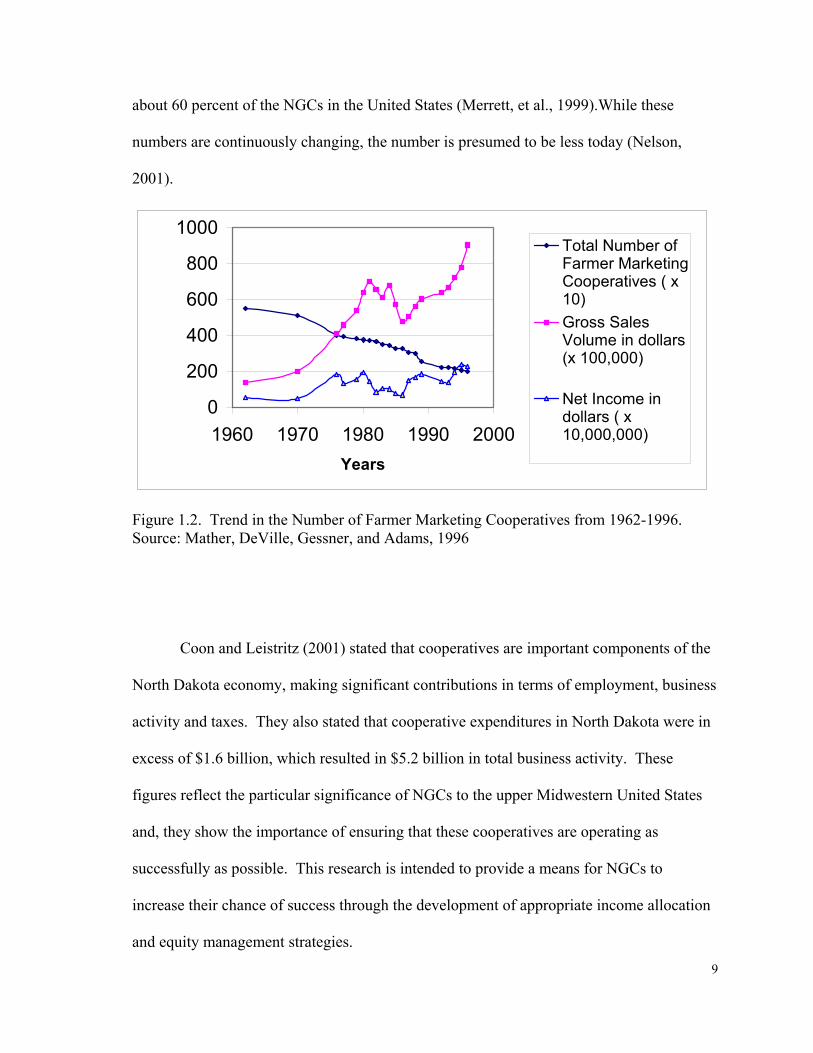
of NGCs on a nationwide scale. However, national trends for farmer marketing

cooperatives, which include but are not limited to NGCs, have shown steady declines from

around 6,000 in 1957 to 3,000 in 1996 (Mather et al.,1998). During this same period of

decline, the gross sales volume associated with these cooperatives has grown in real terms

from $100 million to $900 million. Also, the combined net income generated from these

cooperatives has increased from about $500 million to about $2.2 billion (Mather et al.,

1998 ). Figure 1.2 (next page) shows that, although cooperative numbers have decreased,

their contribution to the economy has continued to grow. Also, the size of cooperatives has

grown to the point where individual cooperative failure may have an even greater impact

on the economy than ever before.

To examine financial impact NGCs more specifically, one can focus on the states

that have seen the most NGC activity. According to a study conducted in 1999, Minnesota

had 29 NGCs present in the state, and North Dakota had 24. Together, they combine for

9

about 60 percent of the NGCs in the United States (Merrett, et al., 1999).While these

numbers are continuously changing, the number is presumed to be less today (Nelson,

2001).

0

200

400

600

800

1000

1960 1970 1980 1990 2000Years

Total Number ofFarmer MarketingCooperatives ( x10)Gross SalesVolume in dollars(x 100,000)

Net Income indollars ( x10,000,000)

Figure 1.2. Trend in the Number of Farmer Marketing Cooperatives from 1962-1996. Source: Mather, DeVille, Gessner, and Adams, 1996

Coon and Leistritz (2001) stated that cooperatives are important components of the

North Dakota economy, making significant contributions in terms of employment, business

activity and taxes. They also stated that cooperative expenditures in North Dakota were in

excess of $1.6 billion, which resulted in $5.2 billion in total business activity. These

figures reflect the particular significance of NGCs to the upper Midwestern United States

and, they show the importance of ensuring that these cooperatives are operating as

successfully as possible. This research is intended to provide a means for NGCs to

increase their chance of success through the development of appropriate income allocation

and equity management strategies.

10

Contribution of the Study

A large body of literature that discusses the unique characteristics of NGCs has

been developed. There are studies specifically discussing NGCs’ unique tax liabilities,

membership structure, and goals. Also, there has been much work done that analyzes the

capital structuring and income distribution decisions of corporations and traditional

cooperatives. However, there have been no studies that incorporate the unique income

allocation options of NGCs under conditions of risk to analyze ways for NGCs to structure

themselves financially and allocate their income in order to maximize membership utility.

Therefore, this study will be useful to the academic community as it is a contribution to the

available literature. The study will also be useful to policy makers involved in supporting

agriculture through value-added initiatives by providing guidance on financial management

issues of NGCs. Finally, the study will provide valuable tools to the managers and member

directors of NGCs when they plan and implement their income allocation and capital

structuring strategies.

Objectives of the Study

The goal of this study is to analyze the impact of NGC’s income allocation

strategies under alternative risk conditions. The specific objectives to meet the goal of this

study are as follows:

Objective 1

Develop an inventory of financial strategies used in the management of the NGCs.

For this objective, historical financial information will be gathered on those NGCs that

11

have made their financial information publicly available through securities and exchange

filings, and a comparison of varying allocation strategies is provided.

Objective 2

Analyze the impact of alternative financial management strategies under specific

risk considerations. This objective will be accomplished by developing a stochastic

simulation model that explicitly incorporates input and output price risks with risk

preferences of NGCs. This NGC simulation model will also be used to explore the

probability of equity and financial stability under various options and allocation strategies

over time.

Methodology

This study uses an expected utility framework to evaluate the optimal allocation

strategies of NGCs under alternative risk considerations. The model will view member

utility as a function of the mean and variance of the NGC’s return on equity. Collins (1985)

initially developed this framework to examine farmer responses to government policies

aimed at reducing business risk in agriculture. His model evaluates return on equity as a

factor of the firm’s leverage decision along with its mean and variance of return on assets.

Collins’ model was extended by Parcell et al.(1990) to incorporate two stochastic variables,

interest rates and return on assets, to evaluate their effect on optimal solvency conditions.

The stochastic simulation model developed in this study is similar to the Parcell et al model

with the exception that allocation strategy is a choice variable. Analysis is conducted to

find the member’s stock value at risk and the probability of equity loss for various levels of

income allocation and lengths of revolvement periods. A comparison of the stochastic

12

simulation model and a value at risk model is performed to validate the findings from this

study.

Organization of the Thesis

This thesis is separated into five chapters. Chapter I is an Introduction to the study

containing an overview of NGCs and their distinctive features that motivate this study.

Chapter II presents a review of the pertinent literature regarding NGC structure, risk

management, and financial management strategies. Chapter III discusses the framework

and model that are used to analyze allocation strategies of NGCs under alternative risk

conditions. Chapter IV presents the results of the study. The conclusions and

recommendations are presented in Chapter IV.

13

CHAPTER II

LITERATURE REVIEW

The purpose of this chapter is to review pertinent literature on the financial

structuring of NGCs. This chapter will be divided into four sections. The first section will

examine the various risks NGCs are exposed to and will review literature aimed at

characterizing these risks. The second section will review literature on the effects of risk

on the financial structure of businesses. The third section examines the effectiveness of

dividend policy as a financial management tool. The fourth section discusses the unique

characteristics and tax implications of NGCs.

Risk Identification and Measurement

Risk Exposure of NGCs

Like other forms of businesses, each NGC will need to analyze itself and the

industry it operates in to determine its optimal financial structure. To do this analysis, a

NGC needs to look at its business risk, financial risk, tax position, and financial flexibility

(Brigham, 1995). Business risk can be defined as all risks that are independent of a NGC’s

financial structure and financing sources (Gabriel and Baker, 1980). Under this definition,

business risk will include things such as unanticipated variations in demand, sales prices,

input prices, and real estate prices (Barry et al., 1995). Business risk also includes the

ability of a NGC to adjust its output prices to account for changes in its input prices and the

extent to which its total costs are fixed (Brigham, 1995). Table 2.1 shows examples of

business risks that selected NGCs have reported in their annual reports.

14

Table 2.1. Business Risk Comparison of Dakota Growers Pasta and American Crystal Sugar Cooperative Business Risks New Generation Cooperatives

Dakota Growers Pasta American Crystal

Sugar Design and Construction Risks X X Input Price Risks X Output Price Risks X Unexpected Cost Overruns X Input Quality X Input Quantity X Government Regulation Affecting Market Prices X Industry Competition X X Weather X X Investments in Other Ventures X Source: Dakota Growers Pasta and American Annual 10-K Securities and Exchange Filings, 1994-2000 and Crystal Sugar Cooperative’s Annual 10-K Securities and Exchange Filings, 1994-2000 It is apparent from Table 2.1 that NGCs have several sources of risk inherent in

their business. Also, each NGC will be affected by a combination of business risks that are

unique to the cooperative. The next section will show how these risks can be characterized

and measured.

Business and Financial Risk Measurement

Barry and Robison (1987) measured business risk as the standard deviation of the

rate of return to a portfolio of risky assets divided by the expected return on those assets.

Escalante and Barry (2001) modified this definition to fit a corporate entity. They modeled

business risk as the standard deviation of a company's return on assets divided by the

expected value of return on assets. Their model is

ROA

ROA

µσ

BR = , (2.1)

15

where

BR=Business risk

σROA= Standard deviation of the return on assets

ROAµ = Mean return on assets (Note: Contrary to accounting practice, Barry (1995)

defines return on assets as net income before tax and interest costs divided by total

assets).

For the managers, members, and investors, quantifying their total exposure to

business risk is a difficult task because there are so many sources of uncertainty and each is

difficult to measure (Olson, 1999). However, arriving at an accurate measure of business

risk is important for NGCs when making capital structuring decisions. Financial theory

states that a business’s optimal capital structure position will change as its business risk

changes. For example, as business risk increases, a NGC should change its capital

structure by lowering its leverage (debt to equity) ratio (Barry and Robison, 1987).

Conversely, if the business risk of the NGC were to decrease, raising its leverage ratio

would be appropriate.

Financial risk can be defined as the added risk placed on the owners of equity that

results from the fixed financial obligation associated with the use of debt financing

(Gabriel and Baker, 1980). Otherwise stated, financial risk is the additional risk that is

placed on NGC members as a result of financial leverage (Brigham, 1995). By using debt,

rather than equity, to operate and grow, a firm is able to have fewer members. Having

fewer members in the cooperative means that each member will receive a greater portion of

income in good times and bear a greater portion of the losses in bad times. Therefore,

financial leverage leads to greater fluctuations in member returns. Financial risk can,

16

therefore, be viewed as a multiplier of business risk where total risk is equal to business

risk times financial risk (Barry and Robison, 1987).

Escalante and Barry (2001) measured financial risk as

−

=

EqDD

EqAµ

EqAµ

FR

ROA

ROA

, (2.2)

where

FR= Financial risk

A= Total assets

Eq= Total equity

ROAµ =Mean return on assets

D=Fixed debt service payments.

By multiplying business risk (equation 2.1) by financial risk (equation 2.2)

Escalante and Barry (2001) arrive a measure of total risk that is represented as

−

==

EqDD

EqAµ

EqAσ

µσTR

ROA

ROA

ROE

ROE (2.3)

where

TR= Total risk

σ ROE= Standard deviation of return on equity

ROEµ = Expected return on equity.

As previously mentioned, an increase in business risk leads to lower levels of

optimal financial leverage. From their definition of financial risk, Gabriel and Baker

17

(1980) show that financial leverage, or use of debt, is the cause of financial risk. By

combining these two statements, one can conclude that optimal financial risk will change

inversely to business risk. That is, as a NGC’s business risk increases, its financial risk as

derived in equation 2.3 will decrease. These findings again point to the importance of

NGCs recognizing the risks in their industry when making financial structure decisions. It

is also important for NGCs to recognize that their optimal capital structuring may change

over time (Jensen and Langemeier, 1996). For example, if a NGC experienced a

significant structural change in its industry, perhaps new competition, causing the company

to face greater levels of business risk, its optimal leverage position would decrease. Thus,

according Gabriel and Baker’s (1980) framework, its financial risk should decrease in

response to an increase in business risk. In this sense, optimal capital structure is not a

fixed point but rather a moving target that reflects the ever-changing risk factors inherent in

a NGC’s operating environment.

Macroeconomic Factors that Expose NGCs to Risk

In the large body of literature discussing capital structure, risk management, and

cooperatives, many sources of risk have been identified. Variability in input prices, output

prices, and demand are all risks that fit into the definition of business risk for a NGC

(Jensen and Langemeier, 1996). However, in quantifying the total risk of any form of

business, it is important to consider the macroeconomic factors that will impact that

business’s overall risk. Macroeconomic factors, such as economic conditions of the United

States and its trading partners, will affect the business risks of a NGC. These factors

influence the magnitude of business risk, and therefore, the optimal financial structure of a

NGC. Swings in economic conditions from times of economic growth to recessions will

18

also affect how a NGC should be structured. It is important to recognize that income

allocation strategies planned during good times will also need to account for the possibility

of economic downturns if those strategies are going to be maintained.

Optimal Solvency Studies

In his article, Collins (1985) sets up a structural model to represent the leverage

decision of agricultural producers. He includes business risk, expected return from farm

operations, capital gains on land, and interest cost of debt in his modeling. His article

examines the effectiveness of agricultural programs that are designed to reduce farm risk

by reducing business risk. Collins’ contribution is the development of a Return on Equity

(ROE) model that looks at optimal leverage decisions from the producer’s perspective. His

results show that, as business risk decreases, the optimal leverage ratio will increase. By

incorporating the notion of risk balancing, Collins finds that the government’s goal of

reducing risk through government programs will be ineffective. Collins’ modeling of

business and financial risk will serve as part of the core framework for this study.

Barry and Robison (1987) use a similar framework to review and incorporate the

concepts of portfolio theory, risk balancing, and equilibrium analysis to analyze financial

structure issues at the firm level. Barry and Robison advance Collins’ work by appraising

the possible changes in interest rates, return on assets, and a change in investor’s attitude

toward risk.

Featherstone et al. (1988) also examined the issue of the government’s farm

policies. In their study, they modify Collins’s model to obtain the optimal leverage ratio

for agricultural producers. They also furthered his modeling by analyzing the effect of

farm policies on the probability of equity loss using a cumulative density function of the

19

rate of return on equity. From there, they demonstrate situations in which the farm policies

can have a positive or negative effect on a producers’ likelihood of receiving positive

returns to their equity. Their conclusion is that policies intended to make farming less risky

may have actually contributed to the financial fragility of agriculture in the early 1980s.

In their article, Parcell, et al. (1990) further Collins’ work to examine agricultural

cooperatives. In their modeling, they include interest rate as a second stochastic variable in

the model. From here, they derive the optimal solvency function and analyze the effects of

changes in business risk and interest rate risk on the optimal solvency of the cooperative.

They also differentiated the optimal solvency equation with respect to mean return on

assets and interest rates. They found that an increase in the variance of interest rates, the

variance of return on assets, and the average interest rate had a negative effect on the

optimal solvency position. These results are a base for hypothesis of this study. However,

their study focused on traditional cooperatives and did not account for unique tax impacts

and differing allocation options of NGCs. Their model will be modified to include these

characteristics to determine the appropriate allocation strategies for NGCs. Also, their

model did not consider unique risks faced by each cooperative. This study will examine

multiple NGCs individually to account for their unique risks.

Dividend Policy as an Effective Financial Management Strategy

for NGCs

NGC income allocation decisions are similar to dividend payment decisions for

corporations. Both payments represent a return to their members’ investments. Because of

their similarities, it is relevant to review the theories that have been offered regarding

20

dividend policy as a tool for managing financial structure. This study will review three

primary theories regarding dividend payment strategies. They are the signaling theory, the

pecking order theory and the dividend irrelevance theory.

Signaling Theory

Signaling theory states that investors regard dividend changes as signals of

management's earnings forecasts (Brigham, 1995). If members received a higher dividend

payment than expected, the NGC’s stock value would rise. The rise in stock value is

because investors are pleasantly surprised by their dividend payment and would regard it as

a signal from management that the business is doing well and that strong returns are

anticipated in the future. Proponents of the theory back this argument by noting that a

company does not want to distribute less to its members than it did in previous years. By

increasing a dividend payment, the company is signaling that it expects to maintain a

higher dividend payment in the future. This theory relates well to NGCs in that

management does not like to change income allocation strategies significantly from one

year to another unless it thinks that the change will be appropriate for many years into the

future. Otherwise, it is likely that members will become dissatisfied about not having a

certain income stream that can be used in budgeting their operation’s future cash flows and

arrive at values for their NGC stock. (Richard, 2001). The important point to draw from

this theory is that NGCs receive pressure from membership to maintain a consistent

dividend policy. So, making a significant change in the policy will affect their members’

expectations of returns in the future.

21

Peking Order Theory

The second theory is referred to as the pecking order theory. This theory states that

the capital structure of a NGC reflects the preferences of the business to fund itself through

internal equity, or retained earnings (Barry et al., 1995). The pecking order theory states

that a business wishes to source capital in the following order:

1) Retained Earnings Internal Equity

2) Debt

3) Convertible Debt

4) Issuing New Equity (Meyers, 1984).

Proponents of this theory give two main reasons for this ordering. First, differing

transaction costs will raise the cost of acquiring capital. Managers will opt to raise capital

using the source of debt with the lowest transaction costs if possible. Retained earnings

will have little or no transaction costs because they are available at the discretion of

management and the board of directors. After retained earnings, the transaction costs

increase with each alternative form of capital until the option of issuing new equity is

reached.

The second reason for the ordering is that asymmetric information between the

manager and individuals interested in offering financial resources will add extra costs to

raising capital. The added costs are a result of the management bearing the added expense

of informing the issuers of capital about all relevant information before capital can be

acquired and throughout the term of capital usage. However, if NGC managers can acquire

needed capital through retained earnings, they will bear no added cost of informing

investors or lenders. The ability of these managers to be able to raise capital without

22

having to inform new investors makes it the least costly source of capital. If debt is used,

managers must keep their lenders informed about the financial position of their NGC at all

times. If the NGC must raise new equity, the cost of informing the public is even greater as

the management will need to inform any prospective investors. Also, for NGCs with

members from multiple states or countries there may be the added cost of having to file

with the Securities and Exchange Commission. This theory fits well with the NGC

structure. It has been observed that NGCs will try to fund their working capital needs

primarily through retained equity. Debt financing is also used quite often, but managers

have viewed it as a secondary source. NGCs have gone back to their members for equity

capital. However, raising new equity capital can only be done in situations where excess

operating capacity is present or a plant expansion is planed.

Dividend Irrelevance Theory

Miller and Modigliani (1961) originally developed the third theory, referred to as

the dividend irrelevance theory. The dividend irrelevance theory advances the notion that a

firm's dividend policy will affect neither the current price of its shares nor the total return

to its shareholders (Miller and Modigliani, 1961). Instead, they argued that a firm is valued

only by its basic earnings power relative to its business risk. However, this theory included

several assumptions that do not hold in the case of NGCs. There are two assumptions that

are inconsistent with the characteristics of NGCs. The first is that personal and corporate

income taxes are left out of their analysis. The second is that the firm’s structuring policy

is independent of its dividend policy. This study’s view conflicts with the dividend

irrelevance theory with regards to NGCs. The theory of this study is that dividend

payments for NGCs will matter for several reasons. First, NGCs have revolved retained

23

earnings without adding any return on the invested funds. Therefore, the net present value

of the revolved earnings in seven years is less than the original value when it was allocated.

For example, if $100 were to be held as qualified retained earnings to be paid to members

on a 7 year redemption schedule at a discount factor of 8 percent is placed on members’

investments, then members will place a value of only $58 on every $100 that is placed in a

reserve account. The second factor that makes dividend policy relevant is that there are

some forms of income allocations that result in members paying taxes oin the current year

regardless of when the money is actually paid to them. But, there are other allocation

options that postpone the members tax liability until the year the actual payment is

received. Therefore, the NGC’s choices of allocation strategies will surly make a

difference to farmers in covering cash flow needs. Members are likely to become

dissatisfied to allocation strategies that allow members to be taxed for income that has not

been received. Along with that, they will be paying dollars today for money that, because

of inflation and time preference of money, is worth less to them in the future. The third

reason that dividend policy is relevant is that a membership utility is based on a

combination of return and risk. By retaining earnings as a source of capital rather than

using debt, the NGC can decrease its financial risk (Parcell et al., 1990). The reduction in

risk will have a positive impact on member utility. However, the lower leverage may lead

to lower returns, which would then have a negative impact on member utility. Therefore,

depending on the members’ risk preference and the effect that leverage will have on

earnings, a change in dividend policy may have varying effects on member utility.

24

Unique Characteristics and Tax Implications of NGCs

Poray and Ginder (1997) state that NGCs differ from traditional cooperatives in

both their structuring and in their underlying motivation. Knapp (1973) stated that the

original form of cooperatives that emerged in the 1920s and 1940s was created as a means

for producers to gain market power by collectively marketing their products and purchasing

their inputs. However, Kelly (2000) states that NGC’s primary objective is to provide

member/producers with additional returns on their raw products through investment in

value-added activities, such as processing and marketing.

It can be debated as to whether the objectives of traditional cooperatives and NGCs

are fundamentally different. However, one large difference that can be offered as a reason

for the new financial structure is that there are a greater number of personal investment

options available today that were unavailable to most agricultural producers 50 or more

years ago during the formation of the elevator and other cooperatives. Because producers

have so many ways to invest their money, it becomes more difficult for cooperatives to

raise large sums of capital through producer investments as was done in the past.

Today, producers need to feel that their investment in a cooperative will be a better

investment than investing in a portfolio of stocks and bonds. Therefore, cooperatives need

to adopt a new structure that allows them to maintain their tax advantages while being able

to entice capital investment funds from members. These features make the financial

structuring decisions unique for NGCs compared to traditional cooperatives and other

business structures. These features are delivery rights that are tied to the level of equity

invested, closed membership, greater up-front equity investment, transferability and the

opportunity for appreciation or depreciation in the value of delivery rights, and higher

25

levels of cash patronage refund. Also, NGCs have unique taxation status that affects their

allocation decisions. Because these unique characteristics play a key role in determining

the financial management strategies of the NGC, they are discussed in detail in the

following section.

Delivery Rights

According to Bielik and Olson (2000), equity shares in a NGC not only assign

membership to producers, but they also allocate delivery rights and obligations. Producers

will purchase equity shares that obligate them to deliver a certain amount of farm product

to the NGC each year. Also, the contract obligates the NGC to accept the product. By

tying delivery rights into the contracting arrangement, an NGC is better able to motivate

members to make the up-front investment needed to provide initial equity capital to the

cooperative. Also, the contract agreements specify that any patronage refunds generated by

the NGC be distributed to members according to the amount of product they delivered to

the NGC.

Stefanson et al. (1995) state that NGCs are structured using a "two-way" contract

that requires the cooperatives to accept a specific amount of product from the producer.

The contract also requires the producer to deliver the same amount of product based on the

number of shares the producer owns. By using delivery rights, producers are guaranteed a

market for their product. Also, the NGC is assured a steady source of input for production.

However, there are quality standards stated in most contracts. If a member cannot meet his

or her delivery requirement with his or her own product, then the cooperative will purchase

the required amount of commodity from other sources to satisfy the contract. This cost is

26

then charged to that member’s account. Then, when dividends are distributed, the

member’s returns will be reduced.

There are usually two or more types of shares issued by an NGC. There are shares

that allocate delivery rights which, for simplicity, will be referred as delivery right shares.

Also, there are shares that allocate voting rights, which will be referred to as membership

shares. Each individual producer may hold only one membership share but can hold

several delivery right shares. There is usually a maximum and minimum investment in

delivery right shares that prevents members from acquiring too large or too small of a stake

in the cooperative. The membership share represents the member’s voting rights;

therefore, each member producer only has one vote, regardless of how many delivery right

shares he owns. Thus, membership structuring keeps NGCs consistent with the democratic

principle of one member, one vote that characterizes most traditional cooperatives. The

cost of a membership share is typically a nominal amount. However, to become eligible to

buy delivery right stock, you must first become a member, which requires owning a

membership stock. Because members are making substantial investments in delivery right

stock, they have expectations of receiving positive cash flows from their investment.

Therefore NGCs must carefully evaluate how much income should be retained on a yearly

basis. If they choose to allocate too little in cash, members will become dissatisfied.

Membership dissatisfaction can cause many internal problems and make it more difficult to

have future equity drives.

The decision on the amount of delivery shares to be issued is addressed during the

feasibility studies done prior to the startup. Once an efficient plant capacity is known, the

amount of product that can be delivered is fixed. Also, at this time, the amount of shares is

27

also fixed, with each share representing delivery rights to a specific amount of product.

The price of the share can then be determined by dividing the total amount of capital the

cooperatives want to raise by the number of shares issued or by the capacity of the plant.

This contracting arrangement works particularly well for processing cooperatives that value

having a fixed amount of though-put arranged in advance. However, cooperatives having

members without a secondary market for their product, such as sugar beet processing

cooperatives, may have a slightly different arrangement whereby a share entitles delivery

rights of a set amount of acreage, rather than a set amount of product (Black et al., 1999).

This setup ensures that the producer’s entire crop is accepted by the NGC.

Closed Membership

While most traditional cooperatives will accept new members at any time,

membership in a NGC is fixed once it has secured its desired level of equity funds and

input capacity. Once the delivery shares are fixed, non-members will be unable to

purchase shares from the cooperative. Their only means of acquiring delivery stock is to

purchase existing shares from a current member. By fixing the amount of outstanding

shares and the delivery commitments per share, the NGC secures a stable product supply.

Even during membership changes when producers sell their delivery right shares, the

supply of product being delivered to the cooperative stays fixed at the original level. This

feature offered by NGCs is necessary in the processing industry. Also, sales of shares

between producers typically require approval from the board of directors before they occur.

This requirement is to ensure that the producer who wishes to acquire available shares

meets all the criteria required to be a member. It also prevents members from having too

many or too few shares.

28

Greater Up-Front Equity Investment

While traditional cooperatives usually charge a nominal yearly fee to patronize the

cooperative, NGCs require a substantial up-front investment to participate in the

cooperative. As an example, the average initial member investment for Dakota Growers

Pasta Cooperative in 1992 was about $11,500. By tying the delivery rights to the amount

of stock owned, cooperatives can more easily motivate producers to make the equity

investments needed, as investment is required for participation (Campell, 1995). Producers

who wish to participate in the NGCs must provide up-front capital for the right to deliver

their commodities to the cooperative. This capital is paid in the form of delivery shares.

NGCs will usually require a producer to own a minimum number of delivery right shares to

be a member.

The higher equity investment can also act as a screening mechanism to ensure that

members are committed to their role in the cooperative. Ensuring that members are

committed is important as their commitment to quality and quantity is key to the success of

the processing plants. For example, if an NGC requires members to purchase specific

assets for their production of the contracted commodity, having committed members is a

necessity.

By receiving high levels of equity financing at the onset of their operations. NGCs

gather the needed equity prior to beginning operations. Therefore, they are not dependent

on retained patronage earnings to supply their membership equity capital (Kelly, 2000).

Having a higher equity outlay at the startup of the company puts them in a position to

return a greater portion of their patronage refunds in cash to their members, rather than

retain them in the business as additional equity financing (Bielik and Olson, 2000). Also, if

29

an NGC decides to expand its operational capacity, a common strategy has been to return

to the membership for additional equity investments. Usually, in such cases, members will

be offered first chance at the sale of new shares. Then, there are still shares unsold they

will be offered to the public. Shares are sold in this fashion so that members do not worry

about diluted shares. Rather, members may be able to turn around and sell the shares for a

realized gain. However, this strategy will work only if members have been satisfied with

their returns up to this point. If the membership were dissatisfied because of low

dividends, it would be difficult to convince anyone to invest in more stock shares.

Transferability of Delivery Rights

Once the initial shares have been sold, they can be traded among members and sold

to prospective members subject to board approval (Stefanson et al., 1995). Although they

are not traded on an open market, the price of shares should reflect the net present value of

the returns members expect to receive from the cooperative over a period of time (Kelly,

2000). However, the lack of marketability can lead to liquidity concerns and, hence,

reduction in share values (Longstaff, 1995). Also, with its privately traded market, NGC

stock prices may vary significantly from one transaction to another as shares are negotiated

between the two parties and prices are not publicly known. This private market is in

contrast to publicly traded market where the stock prices are set by large numbers of buyers

and sellers who are well aware of the market price and the stocks’ price history. If the

NGC is doing well and the prospective buyer sees high earnings potential from owning the

delivery rights, then he or she may agree to a price that is higher than that originally paid

by the member. In this case, the member would realize a gain from the appreciation of the

share value. However, if the producer finds that the earnings potential is low, the shares

30

might have decreased in value for the member. Share prices should therefore fluctuate

according to the performance and earnings expectations of the cooperative.

Higher Levels of Cash Patronage Refund

The financial management strategies of NGCs are noticeably different than those of

traditional cooperatives. NGC management strives to address what producer members

perceive as shortfalls for traditional cooperatives. From the member perspective,

traditional cooperatives have not allocated the desired percentage of earnings. Also, their

retained allocations have not been paid out quickly. The dissatisfaction of membership has

lead producer investors to call for managerial commitments to return a large percentage of

profits to members in the year earned. Also, membership is looking to see shorter periods

for revolving the retained portion of dividends.

As noted earlier, NGCs are being required to raise large amounts of up-front equity

capital. One positive aspect of this requirement is that their low financial leverage results

in a lower financial risk. Also, having the significant amounts of equity relieves the

cooperative of a substantial amount of debt payments. Having the lower debt payments

frees up more of the earnings to be paid out in cash allocations. However, if the

cooperative is successful and has the potential to return higher profits by investing in itself,

debt leveraging should be explored.

Unique Taxation Issues of New Generation Cooperatives

NGCs have several options when deciding how to allocate their income. Several of

these options have differing tax liabilities on both the NGC and its members. Therefore,

these differing tax implications have an impact on a member’s utility and on the cost of

capital for the NGC. Mary Jo Richard of Eide Bailly stated that her firm makes

31

recommendations to NGC clients on equity allocation strategies. Eide Bailly’s preferred

recommendation has been strategies where member-generated income would never be

taxed twice ( Richard, 2001). This statement shows the importance tax laws play in

allocation strategies. The next section describes the differing allocation options of an NGC

and the tax liabilities of each option.

In his discussion of cooperative tax laws, Michael Cook (1995) broke cooperative

taxation down into five categories: Deductions Allowed, Cash Patronage Refunds, Non-

Cash Patronage Refunds, Section 521 Cooperatives, and Unallocated Equity. Each of these

categories will be discussed in the following section.

Deductions Allowed

Michael Cook (1995) initiates his discussion on cooperative taxation by noting that

a cooperative’s goal is to enhance the wealth of its owners through their occupation of

production rather than through their investment. It is by this definition, he says, that a

cooperative is distinguished as an extension of the member producer’s operation. This

distinction is important to remember as the tax advantages of an agricultural cooperative

are linked to its actions and intent. Deductions can be made on some distributions and not

on others. The key is whether the cooperative is distributing patronage income directly to

the members based on their participation.

Cash Patronage Refunds

Cash patronage refunds are the most common form of distribution used by

cooperatives. The amount of the refund distributed to the member is most often based on

the level of patronage given to the cooperative. These refunds are deductible from the

cooperative’s net income in the year that the income is earned. However, the member must

32

include the amount of the allocation in his taxable income in the year received. In our

modeling, this income will be referred to as qualified allocations of cash (QAC).

Non-Cash Patronage Refunds

Non-cash patronage refunds are a way for cooperatives to build equity reserves by

holding some of the members’ refunds in a temporary account. When a cooperative issues

a non-cash patronage refund, its members will be credited with a dollar amount to an

internal equity account. This amount is also based on the amount of business done with the

cooperative. Non-cash patronage refunds can take the form of a qualified notice of

allocation or a non-qualified notice of allocation. If a cooperative issues a qualified notice

of allocation, it may deduct the dollar amount from net income. In this case, the patron

who is issued this allocation must include it in his or her taxable income in the year

received. There are several requirements that must be met for a non-cash patronage refund

to qualify for tax deductibility. They include

1. Paying at least 20 percent of the dividends back in cash and

2. Refunding the total amount of the distribution within 90 days, or

3. Getting consent from the patron to treat the held portion as a distribution that has

been reinvested by the patron.

If the producer gives consent, as required in 3), he will be taxed on the retained

dividends even though he may not receive these payments for several years. This issue has

caused some producers to become unsatisfied with this option. This allocation option will

be referred to as qualified allocations retained (QAR) for this study.

The other form of non-cash patronage refund is known as a non-qualified notice of

allocation. If a cooperative fails to meet the two or more of the requirements listed for

33

issuing qualified notices of allocation, it must use the form of “non-qualified” notices of

allocation. In this situation, the cooperative cannot deduct this amount from taxable

income. Instead, it must pay this amount in the year earned. However, if at a later date, the

cooperative does redeem the held allocation, it may reduce its taxable income in the current

year by the redeemed amount. This redeemed value is now taxable income for the

members in that year. The value of this allocation strategy from the members’ perspective

is that they do not incur a tax liability until the cash is passed to them. However, at the

cooperative level, this form of allocation is more costly because any non-qualified retained

earnings will be taxed. Admittedly, the NGC will receive its tax cost back at the time of

allocation. However, there is an opportunity cost associated with the tax payment that will

be lost. The money initially paid to satisfy the tax liability could have been invested in the

cooperative and earned a return. Therefore, even though the cooperative will be

reimbursed for its tax payment, it will be uncompensated for the lost earnings potential of

that capital. For this reason, NGCs must balance their desire for the most cost effective

sources of capital with memberships desire to stay free of income tax on allocation until the

time of actual cash payment. This allocation option will be referred to as non-qualified

allocations (NQA) in this study.

Section 521

Additional criteria are given in Section 521 of the internal revenue code that, if met,

allow organizations further deductions from their taxable income. The additional criteria

are as follows:

1) Must be an agricultural organization operating on a cooperative basis;

34

2) Producers who use the cooperative must own a majority of the cooperative’s voting

stock;

3) Capital stock cannot pay dividends at a rate higher than the minimum of the legal

interest rate in which it was incorporated, or eight percent;

4) The equity reserves cannot exceed those required by state law or those maintained

for a necessary purpose;

5) The organization must do more business with members than with non-members,

and purchases from non-members cannot exceed 15 percent of the total purchases

by the organization;

6) Permanent records must be maintained that keep patronage and equity balances of

all members and non-members;

7) Members must be given the same advantages in price, inputs, outputs and allocating

patronage refunds to all patrons;

8) Federated cooperatives will be viewed on their structure and activities to determine

whether they qualify for Section 521 status.

When these criteria are met, a cooperative is allowed additional tax deductions. These

deductions can be very beneficial to all qualifying NGCs. These additional deductions

include

1) Dividend payments on capital stock made during the year,

2) Patronage payments derived from non-patronage business, and

3) Amounts paid to redeem non-qualified allocations to patrons from non-patronage

business.

35

Unallocated Equity Any income that is not distributed to patrons is placed in unallocated equity.

Because the members will not directly benefit from this income, cooperatives are taxed at

corporate tax rates for the full amount placed into this account in that year. If a cooperative

decided to distribute the equity out to its members, the income would need to be included

as taxable income for the members. Therefore, this allocation strategy would receive

double taxation costs similar to that of a corporation and its members. Unallocated equity

is only reissued in extreme circumstances. The advantage of this strategy is that the NGC

will have a fixed source of equity that it is not committed to paying out to members. This

allocation option will be referred to as unallocated reserves (UAR) in the study.

36

CHAPTER III

METHODOLOGY AND DATA

The purpose of this chapter is to develop a stochastic simulation model that uses

financial data, such as retu`rn on assets business risk, financial risk, and cost of debt, to

facilitate financial allocation decisions for NGCs. A methodological contribution of this

study is to explore optimal solvency, a financial performance measure, as a tool to guide

financial management strategies. This chapter is separated into two sections. The first

section discusses the development of the Theoretical Model used to develop optimal

solvency in past studies. The second section extends the optimal solvency model to

explicitly incorporate allocation strategies and uses comparatives statics to explore the

relationship between optimal solvency, allocation strategy, and the probability of equity

loss.

Theoretical Model

One of the primary goals of NGCs is to distribute the highest possible returns to

members while still maintaining adequate amounts of internal reserves to be used for

working capital and as a safety net in times of adverse economic conditions (Daiz-Hermelo

et al., 2001). This study evaluates how NGCs can make income allocation decisions to best

meet these goals under business and financial risk. Distributions for return on equity

(ROE), interest cost of debt (K), and covariance of ROE and K will be used to determine

the optimal solvency for NGCs.

37

Return on Equity Modeling

This section builds on the models developed by Collins (1985) and Parcell et al.

(1990). Collins’s model focused on finding the optimal leverage given the levels of

business and financial risk and the risk aversion of the farmers. In his study, Collins

measures ROE as follows:

L11] LKi

Ar

[R pE −

⋅−+= , (3.1)

where

RE = net return on equity

rp = net expected return to the company

A = total assets

i = expected increase in asset value

K = interest cost of debt

L = ratio of debt to assets (leverage ratio).

Collins (1985) defined AR as the expected gross return on assets including

inflation and substituted AR for iArp + . He then modeled the expected return on assets as

a normally distributed function with a mean of R A and a variance of σA2 . The expectation

and variance of ROE can now be written in equations 3.2 and 3.3 as

L11] LKR[R AE−

⋅−= (3.2)

38

22A

2E L1

1σσ

−= (3.3)

Parcell et al. (1990) extended Collins’s work to account for uncertainty in interest

rates on debt. They did so by treating interest rates on debt (K) as a stochastic variable. By

treating interest rates as a stochastic variable, the expected stochastic rate of return on

equity (equation 3.2) changes to

L11] LKR[R AE−

⋅−= ,. (3.4)

While the variance of return on equity (equation 3.3) becomes

( )2KA,

2K

2A2

E L1γσσ

σ−

−+= , (3.5)

where

σ2K = standard deviation of interest rate on debt

γAK = covariance of return on assets and interest rate on debt.

Expected Utility Maximization Modeling

By assuming the conditions of normality, RA~N )σ,R( 2AA , K~ )σ,K( 2

K and

constant relative risk aversion coefficient, Parcell et al (1990). demonstrate how a negative

exponential utility function can be used to arrive the expected utility maximizing solution

by maximizing

( )

−

⋅−⋅⋅

−

−⋅−

= 2KA,

22K

2AA

L12LγLσσ

2ρ

L1 LKRV(L) , (3.6)

where

ρ = Pratt-Arrow coefficient of decreasing absolute risk aversion.

39

The first-order conditions for equation 3.6 are presented in equation 3.7.

( )( ) ( )

0L1

L)(1γLσσρ

L-1LKR

L1K

L(V(L))

3KA,

2K

2A

2A =

−

+−⋅+−

⋅−+

−−

=∂

∂ (3.7)

Solving equation 3.7 for the optimal leverage ratio (L*) yields

KA,2KA

KA,2AA*

γρσρKRγρσρKR

L⋅−⋅+−

⋅+⋅−−= (3.8)

Setting AKKA,KA, σστγ ⋅⋅= where KA,τ is correlation between the RA and K, equation 3.8

can be rewritten as

)στ(σσρKR)στ(σσρKR

LAAKKKA

KAKAAA*

⋅−⋅+−

⋅−⋅−−= (3.9)

Leverage (L) is measured as EquityDebt . While solvency (S), can be measured as

AssetsEquity . The identity Assets=Debt +Equity can be used to show that S = 1-L. Therefore,

optimal solvency can be written as such.

⋅−⋅+−

⋅−⋅−−−=

)στ(σσρKR)στ(σσρKR

1SAAKKKA

KAKAAA*

)στ(σσρKR)σσστ2ρ(σ

AAKKKA

KKAAKA

⋅−⋅+−

+⋅⋅−= (3.10)

Parcell et al.’s (1990) advancement of including stochastic interest rates in the

utility model will be significant to those NGCs that have sizable portions of their debt

obligations as short-term or variable interest rate obligations. It is also significant in that

the financial structuring decision will affect the interest costs of debt.

40

This study extends equation 3.10 by incorporating NGC’s unique income allocation

decisions and tax obligations and by exploring relationships that can assist NGC

management to make efficient financial management decisions.

Optimal Solvency and Allocation Decision Model

From equation 3.10, return on assets can be modeled as:

nn

nnnA DEq

DKNIBTR+

⋅+= , (3.11)

where

NIBTn = net income in the current period before taxes are deducted

Kn = weighted average interest cost of debt

Dn = total debt

Eqn = total equity for the current period, and

Dn = total debt for the current period.

For further detail on NIBITn, see Appendix C.

For NGCs, total equity can be written as

),Qar%(NIBT)}T)(1Nqa%{(NIBT)}T)}(1Uar%NIBT%Nqa{NIBT

%)Qar(NIBTUarNqaQarPicCsEq

xnxnxnxnxn

nnnnn

nnnnnnnn

−−−−− ⋅−−⋅−−⋅+⋅+

⋅+++++=

(3.12)

where

Csn =the balance of common stock for the current period

41

Nqa%n = the percentage of NIBT that is allocated to a non-qualified allocation

account at the end of the current period

Pic n = the balance of paid in capital for the current period

UAR% n = the percentage of income that is placed in an unallocated reserve

account at the end of the current period

Qarn, = the current balance of the qualified allocations redeemed account

Nqan = the current balance of the non-qualified allocations account

Uarn = the current balance in the unallocated reserve accounts.

It will be assumed that the NGC is not going to have new equity drives over the

period evaluated. Therefore, Csn and Picn are fixed and known with certainty. Qarn, Csn,

and Nqan are also known as they represent the observed balances in their respective

accounts. The other variables comprising the equity value are unknown amounts as they

contain the stochastic net income before tax for the current period. By combining

equations 3.11 and 3.12, the return on assets for this strategy can be written as follows:

−⋅−−−−−⋅−−

−⋅+⋅+

⋅++++++

⋅+=

)xnQar%xn(NIBT)}xnT%(1xnNqaxn{NIBT

)nT%}(1nUarnNIBT%nNqan{NIBT

%)nQarn(NIBTnUarnNqanQarnPicnCsnD

DKNIBITR nnn

A (3.13)

This modeling of return on assets reflects NGCs using an “x-year redemption” plan.

For example, if management had a seven-year redemption schedule, the NQA1995 would be

returned in 2002. This model assumes that the revolvement policies are strictly followed.

Such policies are commonly stated in the growers’ agreements of the cooperative by-laws.

42

For example, American Crystal Sugar plans to redeem retained earnings on a seven-year

schedule.

The advantage of this strategy is that members will gain satisfaction by knowing

how long their allocated earnings will be retained and the amount that they will receive

when the earnings are redeemed. The disadvantage is that the management will not be able

to make yearly decisions on how much money can be redeemed without modifying its plan.

This means that if a NGC’s earnings were decreasing, it could face a situation where it was

continually redeeming more equity than it was retaining. Therefore, it would become

under-capitalized unless it changed its allocation strategy to retain a greater percentage of

earnings in the current year.

A second strategy, called the “Percent of All Equities Strategy,” is presented in

Appendix A. In this strategy, management of the NGC sets a specific percentage of the

total equity to redeem each year. This strategy may be appealing in that it helps to

maintain a more stable equity account balance. However, members may dislike this

strategy as it leaves them uncertain about their future redemption payments.

Equation 3.13 is shortened to make it more mathematically friendly such that return

on assets is represented as

Z)F(GT))M)(1BN(BBRDJ

DKBR A −−−⋅+⋅+⋅++⋅+

= , (3.14)

where

B = net income before tax in current period (NIBTn)

K = weighted average interest rate of total debt in the current period

D = total debt for the current period

J = current equity of the cooperative (Csn+Picn+Qarn+Nqan+Uarn)

43

R = qualified earnings allocated and retained to member accounts (Qarn%)

N = percentage of NIBT that is allocated to a nonqualified allocation account

at the end of the current period (Nqan%)

M = percentage of income that is placed in an unallocated reserve account at

the end of the current period (Uarn%)

T = current tax rate (Tn)

C = the percentage of income distributed as cash to members (Qacn%)

F = NIBTn-x%*

G = (Nqan-x%)*(1-Tn-x), and

Z = the current balance of the qualified allocations redeemed account (Qar%n-x).

Equation 3.14 is adjusted to isolate the stochastic variable B so that ROA can be measured

as

Z)F(GT))M)(1(NB(RJDKBR A −−−+++⋅+

= (3.15)

Equation 3.15 can be simplified so that ROA is represented as:

XW)B(RDKB

RA ++⋅+

= (3.16)

where

X = J+D-F(G-Z) = current equity and debt of the NGC minus the equity

redeemed in the current period, and

W = (N+M)(1-T) = new equity from current income allocated in the form of

NQA or UAR.

In this next section, the study will derive the expectation of the members return on

assets given these allocation decisions. Expected Return on Assets is shown as

44

++

⋅+

++

==XW)B(R

DKEXW)B(R

AER]RE[ AA

XW)(RB

DKXW)(RB

BR]E[R AA++

+++

== (3.17)

By plugging equation 3.17 into equation 3.10, one can arrive at the optimal

solvency for a NGC.

)στ(σσρK)()(

)σσστ2ρ(σ*

AAKKK

2KKAAKA

⋅−⋅+−

++⋅

+

++

+⋅⋅−=

XWRBDK

XWRBB

S (3.18)

Comparative Static Analysis The optimal solvency ratio (S*) can be defined as one minus the leverage ratio

(1-L*). Therefore, differentiating S* with respect to variance of return on assets, variance

of interest rates, and percent of income retained allows for presumptions to be made about

allocation decisions and risk. To sign the comparative static results, it is assumed that the

correlation between the interest rate and the rate of return on assets falls between –1 and 1

and that KA σσ ⋅> . Let Den and Num refer to the denominator and numerator, respectively, in

equation 3.19. To evaluate the effect of σA on S*, differentiate equation 3.18 with respect

to σA to arrive at

2

en

KAKKAKA

DN)*στρ(D2ρ)στ-(σ* ⋅⋅+⋅⋅⋅

=∂∂

A

Sσ

(3.19)

From equation 3.19, one can see that a change in the solvency ratio from a change in the

variance of return on assets has a positive relationship, 0σ

*S

A

>∂∂ . That is, an increase in

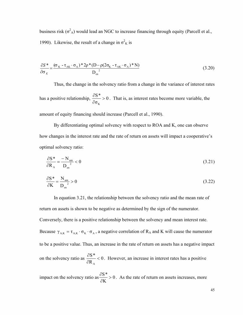
45

business risk (σ2A) would lead an NGC to increase financing through equity (Parcell et al.,

1990). Likewise, the result of a change in σ2K is

2en

AAKKAAKK

DN)*)στ-ρ(2σ(D*2ρ*)στ-(* ⋅−⋅

=∂∂ σσ K

S (3.20)

Thus, the change in the solvency ratio from a change in the variance of interest rates

has a positive relationship, 0σ

*S

K

>∂∂ . That is, as interest rates become more variable, the

amount of equity financing should increase (Parcell et al., 1990).

By differentiating optimal solvency with respect to ROA and K, one can observe

how changes in the interest rate and the rate of return on assets will impact a cooperative’s

optimal solvency ratio:

0DN

R*S

2en

um

A

<−

=∂∂ (3.21)

0DN

K*S

2en

um >=∂∂ (3.22)

In equation 3.21, the relationship between the solvency ratio and the mean rate of

return on assets is shown to be negative as determined by the sign of the numerator.

Conversely, there is a positive relationship between the solvency and mean interest rate.

Because AKKA,KA, σστγ ⋅⋅= , a negative correlation of RA and K will cause the numerator

to be a positive value. Thus, an increase in the rate of return on assets has a negative impact

on the solvency ratio as 0R

*S

A

<∂∂ . However, an increase in interest rates has a positive

impact on the solvency ratio as 0K*S>

∂∂ . As the rate of return on assets increases, more

46

debt financing should be used causing equity financing to decrease. Alternatively, as

interest rates increase, the amount of debt financing should decrease. In such situations,

more equity financing should be used (Parcell et al., 1990).

Differentiating the optimal solvency equation with respect to R (allocation decision)

shows the effect of changes to the percent of income retained on the solvency ratio:

2en

um

D

N*XW)(RB

DKBXW)(RB

BB

R*S ++⋅

⋅⋅+

++⋅⋅

=∂∂ (3.23)

If we assume that net income before tax (B) and interest costs )D(K ⋅ are positive,

then 0*>

∂∂

RS . Under this scenario, an increase in the amount of income retained will

increase the solvency of the cooperative. In equation 3.5, risk, as measured by return on

equity, is shown to change directly with leverage (L). Because solvency (S) can be defined

as (1-L), we can conclude that an increase in solvency will lead to a decrease in risk.

Therefore, an increase in the amount of income retained will increase the solvency of the

cooperative which will reduce its risk.

In this analysis, an NGC is limited to choosing to allocate its income between two

sources. The NGC must either allocate the income in the form of a qualified retained

earning or as qualified cash allocation. So, C = (1-R) or, the percentage of income

allocated as cash, equals one minus the percentage of income allocated and retained.

Therefore, a change in the percentage of income allocated in the form of qualified retained

will have an equal and opposite effect on the percentage of income that is allocated in the

47

form of a qualified cash allocation. Although the choice of a qualified cash allocation does

not explicitly appear in the optimal solvency formula, it can be evaluated as having the

inverse effect of a change in R, or the percentage of income retained. Therefore, the results

are presented from the standpoint of the percentage of income retained rather than from the

percentage of income issued.

48

CHAPTER IV

DATA AND RESULTS

The purpose of this chapter is to describe the data used to analyze the theoretical

framework developed in Chapter III. A description of the Data Sources used in this study

is first presented. Then, an analysis of empirically determined solvency ratios and ROE

sensitivities is presented. The final section of this chapter discusses the effect of changes in

income allocation strategies on the probability of equity loss.

Data Sources

Financial data used in this study comes from two sources: 1) a deterministic

forecasting model and 2) publicly available security and exchange filings. First the

deterministic forecasting model is described.

Deterministic Forecasting Model

The initial deterministic forecasting model (DFM) described in this section was

developed through the work of Mr. Edward Janzen and Mr. Frayne Olsen. The goal of the

DFM is to be able to generate 10 years of proforma financial information in the form of

financial statements, financial ratios, and graphs that can be used as a tool in evaluating

income allocation and other planning decisions. This goal will be accomplished by

entering information about the NGC’s past and present financial position, production

characteristics, and allocation strategies along with future sales and price estimates of the

inputs and outputs. Then, business and financial risk will be incorporated into model using

the @risk software. Business risk may come through variation in the estimates of the price

49

of raw materials, the price of goods sold, the quantity of goods sold, the price royalties,

percentage cost of discounts, and the production costs. Financial risk comes, in part, from

variation in interest rates on short-term debt. Another factor adding to financial risk is the

need for NGCs to maintain certain solvency levels that satisfy loan covenants placed on the

businesses by their lenders. The model also allows for constraints to be placed on

allocation decisions that reflect the constraints present in loan covenants.

The DFM is composed of five sections. They are the input section, the intermediate

work sheet section, the financial statement section, the summary data section, and the risk

modeling section. Then, each section is further broken down into subsections. Each

subsection is fitted onto one sheet, with the exception of production and inventory sheets.

Input Section

The input/miscellaneous section contains all input variables: parameters, strategies,

and beginning balances. In many cases, the values beyond the base year can be represented

by explicit entries, or they can be represented by an inflation or growth rate from the base

value. The input section also contains parameters that might not be applicable in specific

cases (i.e., royalties, packaging materials, etc.). This section is separated into six

subsections. They are

1) General Information and Allocation Strategy Data

2) Production, Sales, and Price Data

3) Inventory Data

4) Operating Costs Data

5) Investment and Depreciation Data

6) Debt Service Data.

50

The General Information and Allocation Strategy Data sheet contains entries for the

name of the company and for name of the products produced. This information is placed at

the top of each sheet of the model. Also, this section contains input cells that implement

the income allocation decisions for the NGC over the 10 year planning horizon. These

allocation decisions include the options of allocating income in the form of a qualified cash

allocation, a qualified retained allocation, a non-qualified retained allocation, and/or an

unallocated reserve. Further, there are input cells where any plans to redeem reserve

balances can be entered. The entries into the allocation and redemption cells will affect the

income statement’s calculation of net income after tax and in the current period as well as

net income before tax and the equity balances in the future period. These are the cells that

this study will be working with most closely.

In the Production, Sales, and Price Data sheet, projected sales volume, input prices,

output prices, discounts, royalties and brokerage fees are entered for the 10 year planning

horizon. Also, production capacity is estimated for the same period of time. The projected

values in this section make up the business risk that will be incorporated in this study. The

capturing of business risk can be done by entering a distribution of values, rather than a

single value, into the these input cells.

The Debt Service Data sheet contains input cells to represent both long-term loans

and a short-term revolving line of credit. To calculate the interest costs on the revolving

line of credit, the model has input cells to project the interest rate on the revolving line of

credit for the 10-year planning horizon. The uncertainty in this interest will also be

represented as a distribution of possible values rather than as a single estimated value. This

representation of a stochastic interest rate makes up part of the financial risk of the NGC.

51

The other input sheets in this model contain input cells for data used to calculate

fixed costs, various balances sheet values (i.e. accounts payable and receivables, inventory

on hand and plant and equipment values), and depreciation for the assets.

Intermediate Worksheet Section

The Intermediate Worksheet Section is made up of various worksheets that need

very little manipulation in terms of changing information for specific NGCs. The only

information that needs to be entered into this section is the state income tax brackets

specific to each individual state, the depreciable life of land buildings, and additional

acquisitions planned over the next 10 years. The sheets in this section are primarily for the

calculation of the values that are entered into the financial statements. This section also

contains six subsections. They are

1) Production and Inventory Sheets

2) Debt Service Sheets

3) Amortization Schedule and Account Balances

4) Depreciation for Book

5) Depreciation for Tax

6) Income Tax Calculations.

The calculations made in Production and Inventory sheets are based on volume and

price forecasts from the Input sheets. Other input parameters influencing production and

inventory calculations are production capacity limits and desired inventory levels. Expense

amortization, fixed asset account balances, changes in accounts receivable and accounts

payable, and net operating loss carryover for tax calculations are all generated in the

Amortization and Account Balances sheet. The Debt Service sheets handle the interest

52

payment on the revolving line of credit, the debt retirement, and interest calculations for up

to five loans. The Book and Tax Depreciation sheets generate book and tax depreciation

calculations using allowable depreciable life of the assets for book basis income statement

and the tax rate depreciation schedule for tax basis income statement. Applicable tax tables

are extracted from page 60 of the 2001 Internal Revenue Service publication number 946

for the tax depreciation sheet. The Income Tax sheet contains input cells to create tables to

match federal and state (North Dakota) income tax tables. This sheet also calculates

federal and state income tax calculations used in the Income Statement.

Financial Statement Section

This section contains five sheets. They are

1) Income Statement calculated from Book Depreciation

2) Income Statement Calculated from Tax Depreciation

3) Balance Sheet

4) Cash Flow Statement

5) Members Equity Statement.

These sheets have been designed to be flexible enough in terminology to fit NGCs

across multiple businesses. However, not all terminology will fit well across industries.

Therefore, minor changes to account titles may be needed to adapt this model from one

NGC to the next. These worksheets were modeled to be comparable with financial

statements presented in Securities and Exchanges filings as well as annual reports to

membership.

Summary Data Section

This section contains 3 sheets. They are

53

1) Financial Ratios

2) Other Ratios

3) Summary Graphs.

The financial ratios presented in this section can be used to view measures of

solvency, liquidity, profitability, and financial efficiency over the 10 year planning horizon.

Also, these ratios may be used as constraints on the allocation decisions, as many loan

covenants will require the NGCs to maintain liquidity and solvency ratios at or above a

specific value. The Other Ratios sheet contains ratios used to measure operating efficiency

and member-level returns. Also, this sheet has ratios that incorporate the time value of

money to view the effects of differing member returns over the 10-year planning horizon.

Finally, a sheet of summary graphs is available to make visual comparisons between

different strategies.

Risk Modeling Section

The risk modeling section allows the user to incorporate uncertainty into the model.

Distributions that model business risk, interest rate risk, and the correlation between them

can be entered. This section also contains cells that will allow the user to change income

allocation percentages and revolvement periods to view their effect on decision variables

such as the solvency ratio, return on equity and standard deviation of return on equity,

probability of equity loss, and value at risk.

Financial information generated from this study’s deterministic forecasting model is

used to demonstrate how the managers of NGCs can use historical information specific to

their company to project future financial performance and anticipate their adequate levels

of solvency to make income allocation decisions. For simplicity, data from the

54

deterministic forecasting model will be given the name of NGC Bean Cooperative, a

hypothetical company.

Security and Exchange Filings

The other three data sets presented in Table 4.1 are taken from the annual 10-k

statements. Actual data from one durum processing cooperative and two sugar processing

cooperatives are used to illustrate that allocation strategies will be unique both across

industries and across individual firms within the same industry. All data for these three

cooperatives were gathered over the time period of 1994 through 2000.

Table 4.1 (next page) shows the data used to calculate the optimal solvency

positions for each of the individual cooperatives. Interest rate data (column seven) and

return on assets data (column nine) are used to create probability distributions and

correlations between the two. Column eight shows the percentage of net income that has

been retained by each NGC. To produce the initial data for NGC Bean Cooperative, it is

assumed that the company has previously followed the strategy of retaining 40 percent of

its income.

Looking at Table 4.1, one can see the distinct differences in financial and risk

characteristics across these cooperatives. For example, it appears that the two sugar

processing cooperatives have historically been charged a lower interest rate on their debt

than Dakota Growers Pasta Cooperative. Also, the sugar cooperatives have had a higher

return on assets along with a higher business risk, as represented by variability of return on

assets.

55

Table 4.1. Summary Statistics by Year for Each NGC (in Thousands)

Period Total Assets Total Debt Total Equity NIBT NIBTAD Int. Rate % Ret. ROA E/A ROE Dakota Growers Pasta Cooperative

1994 $ 45,125 $ 33,018 $ 12,107 $ (208) $ 2,611 8.54% 100.00% 5.79% 26.83% -1.72% 1995 $ 47,842 $ 33,375 $ 14,467 $ 1,408 $ 4,462 9.15% 100.00% 9.33% 30.24% 9.73% 1996 $ 49,894 $ 24,208 $ 25,686 $ 2,622 $ 4,774 8.89% 63.75% 9.57% 51.48% 10.21% 1997 $ 68,739 $ 38,330 $ 30,409 $ 6,926 $ 9,828 7.57% 73.88% 14.30% 44.24% 22.78% 1998 $ 124,537 $ 87,409 $ 37,128 $ 9,374 $16,078 7.67% 49.29% 12.91% 29.81% 25.25% 1999 $ 135,873 $ 76,838 $ 59,035 $ 8,487 $14,096 7.30% 0.52% 10.37% 43.45% 14.38% 2000 $ 131,857 $ 71,198 $ 60,659 $ 6,330 $11,898 7.82% 6.43% 9.02% 46.00% 10.44%

Mean 8.13% 56.27% 10.18% 38.86% 13.01% Standard Deviation 0.72% 40.48% 2.77% 9.67% 9.03% American Crystal Sugar Cooperative

1994 $ 420,000 $ 304,391 $ 115,609 $ 6,653 $ 25,555 6.21% 100.00% 6.08% 27.53% 5.75% 1995 $ 420,890 $ 278,843 $ 142,047 $ 38,517 $ 57,478 6.80% 43.22% 13.66% 33.75% 27.12% 1996 $ 465,136 $ 313,000 $ 152,136 $ 23,397 $ 41,457 5.77% 68.56% 8.91% 32.71% 15.38% 1997 $ 581,504 $ 405,576 $ 175,928 $ 57,100 $ 81,678 6.06% 29.09% 14.05% 30.25% 32.46% 1998 $ 648,118 $ 423,275 $ 224,843 $ 15,143 40,836 6.07% 56.43% 6.30% 34.69% 6.73% 1999 $ 667,824 $ 426,538 $ 241,286 $ 77,402 101,331 5.61% 27.56% 15.17% 36.13% 32.08% 2000 $ 739,719 $ 490,389 $ 249,330 $ 68,095 101,000 6.71% 28.34% 13.65% 33.71% 27.31%

Mean 6.18% 50.46% 11.12% 32.68% 20.98% Standard Deviation 0.44% 26.89% 3.90% 2.90% 11.54% Minn-Dak Sugar Cooperative

1994 $ 74,771 $ 32,967 $ 41,804 $ 5,346 $ 7,426 6.31% 15.61% 9.93% 55.91% 12.79% 1995 $ 99,991 $ 55,917 $ 44,074 $ 24,326 $27,821 6.25% 6.73% 27.82% 44.08% 55.19% 1996 $ 138,270 $ 80,609 $ 57,661 $ 6,958 $11,996 6.25% 19.97% 8.68% 41.70% 12.07% 1997 $ 171,895 $ 100,221 $ 71,674 $ 16,981 $23,425 6.43% 5.58% 13.63% 41.70% 23.69% 1998 $ 184,830 $ 101,981 $ 82,849 $ 13,181 $19,790 6.48% 6.71% 10.71% 44.82% 15.91% 1999 $ 174,296 $ 93,955 $ 80,341 $ 4,180 $ 9,874 6.06% 0.11% 5.66% 46.09% 5.20% 2000 $ 173,001 $ 96,576 $ 76,425 $ 25,616 $32,222 6.84% 0.00% 18.63% 44.18% 33.52%

Mean 6.37% 7.82% 13.58% 45.50% 22.62% Standard Deviation 0.25% 7.49% 7.49% 4.86% 17.02% NGC Bean Cooperative

2001 $ 25,911 $ 10,484 $ 15,427 $ 3,993 $ 4,986 9.47% 40.00% 19.24% 59.54% 25.88% 2002 $ 26,698 $ 10,604 $ 16,094 $ 1,666 $ 2,641 9.20% 40.00% 9.89% 60.28% 10.35% 2003 $ 27,034 $ 10,447 $ 16,588 $ 1,235 $ 2,191 9.15% 40.00% 8.11% 61.36% 7.45% 2004 $ 28,118 $ 10,171 $ 17,947 $ 3,397 $ 4,332 9.19% 40.00% 15.41% 63.83% 18.93% 2005 $ 28,423 $ 9,894 $ 18,529 $ 5,449 $ 6,360 9.21% 40.00% 22.38% 65.19% 29.41% 2006 $ 30,182 $ 9,616 $ 20,566 $ 6,759 $ 7,645 9.21% 40.00% 25.33% 68.14% 32.86% 2007 $ 30,880 $ 9,533 $ 21,346 $ 3,186 $ 4,043 8.99% 40.00% 13.09% 69.13% 14.92% 2008 $ 30,636 $ 9,222 $ 21,414 $ 3,567 $ 4,393 8.95% 40.00% 14.34% 69.90% 16.66% 2009 $ 29,017 $ 8,908 $ 20,109 $ 2,186 $ 2,977 8.88% 40.00% 10.26% 69.30% 10.87% 2010 $ 26,019 $ 8,482 $ 17,538 $ 330 $ 1,083 8.87% 40.00% 4.16% 67.40% 1.88%

Mean 9.11% 40.00% 14.22% 65.41% 16.92% Standard Deviation 0.19% 0.00% 6.59% 3.95% 9.97% Notes: NIBT is the net income before tax; NIBTAD is the net income before tax and debt payments; Int. Rate is interest rate; % Ret is percent retained; ROA is return on assets; E/A is equity to asset ratio; and ROE is return on equity. Estimated average sugar production costs are deduced from net proceeds to arrive at NIBIT. Average interest rates of the NGCs short-term operating lines are used to represent the weighted average cost of capital. One can also use the average cost of debt to arrive at similar results and provide the same conclusions of this study. Source: Dakota Growers Pasta’s Annual 10-K Securities and Exchange Filings, 1994-2000; American Crystal Sugar Cooperative’s Annual 10-K Securities and Exchange Filings, 1994-2000; Minn-Dak Sugar Cooperative’s Annual 10-K Securities and Exchange Filings, 1994-2000. NGC Bean Cooperative data were generated in this study’s deterministic model using hypothetical data.

56

It is interesting to note that American Crystal Sugar’s business risk is 48% less than

that of Min-Dak Sugar’s. These differences will be discussed in more detail as their

impacts on the results are presented.

Results

The Results section is separated into three subsections. The first section shows how

membership’s risk aversion will impact optimal solvency levels and the probability of

equity loss. This section also examines the sensitivity of the cooperative’s optimal

solvency to the risk parameters. The second section demonstrates the effectiveness of

allocation decisions and revolvment length changes as a tool to adjust a cooperative’s

solvency and reduce its probability of equity loss. The third section is a validation of the

results using a value at risk comparison.

Risk Aversion and Optimal Solvency

First, information from Table 4.1 (next page) was plugged into equation 3.7 to find

the optimal solvency ratios for each of the NGCs given their various levels of member’s

risk aversion. Table 4.2 shows the empirically determined solvency ratios for the NGCs. It

also shows the sensitivity of the optimal solvency to changes in ROA, K, Variance of

ROA, and Variance of K.

The risk aversion coefficient used in Table 4.2 and in the following tables ranges

from a value of one to ten, with one representing members who have a low aversion to risk

and ten representing those with a high aversion to risk.

57

Table 4.2. Empirically Determined Solvency Ratios and Sensitivity Analysis of Each NGC

Risk Aversion Coefficient ROE Optimal E/A

Optimal E/A (ROA+S.D.)

Optimal E/A (ROA Var.

*120%)

Optimal E/A (Int. Rate-

S.D.)

Optimal E/A (Int. Var.*

120%) Dakota Growers Pasta Cooperative

1 50.16% 4.88% 2.08% 5.62% 3.62% 4.93% 2 29.29% 9.69% 4.15% 11.17% 7.20% 9.78% 4 18.86% 19.11% 8.25% 22.03% 14.25% 19.27% 6 15.38% 28.28% 12.30% 32.60% 21.16% 28.49% 8 13.64% 37.20% 16.31% 42.89% 27.94% 37.44%

10 12.60% 45.89% 20.26% 52.91% 34.58% 46.14% American Crystal Sugar Cooperative

1 169.30% 3.03% 1.69% 3.65% 2.78% 3.04% 2 87.74% 6.06% 3.39% 7.29% 5.56% 6.07% 4 46.95% 12.12% 6.77% 14.58% 11.12% 12.15% 6 33.36% 18.18% 10.16% 21.88% 16.68% 18.22% 8 26.56% 24.25% 13.55% 29.17% 22.24% 24.29%

10 22.48% 30.31% 16.94% 36.47% 27.81% 30.37% Minn-Dak Sugar Cooperative

1 100.48% 7.66% 3.75% 9.21% 7.40% 7.66% 2 53.40% 15.32% 7.51% 18.44% 14.81% 15.32% 4 29.86% 30.68% 15.02% 36.93% 29.66% 30.69% 6 22.01% 46.08% 22.55% 55.46% 44.55% 46.09% 8 18.09% 61.52% 30.09% 74.04% 59.47% 61.53%

10 15.73% 77.00% 37.63% 92.67% 74.43% 77.00% NGC Bean Cooperative

1 83.10% 9.68% 4.46% 11.63% 9.43% 9.68% 2 46.09% 19.36% 8.92% 23.28% 18.87% 19.36% 4 27.58% 38.77% 17.85% 46.61% 37.78% 38.77% 6 21.41% 58.21% 26.79% 69.99% 56.73% 58.22% 8 18.33% 77.70% 35.74% 93.42% 75.72% 77.70%

10 16.48% 97.23% 44.70% 116.90% 94.76% 97.23% Notes: ROE is return on equity; E/A is equity to asset; S.D. is standard deviation; Int. is interest; and Var. is variance.

By definition, individuals with a low risk aversion are willing to accept an increase

in risk with a smaller increase in expected return than those with a higher risk aversion.

Because every individual has a unique risk aversion, the NGC must try to find the average

risk aversion of membership upon which to base its allocation decision. By comparing risk

aversion coefficients (column one) with the optimal equity to asset ratios (column three), it

is apparent that the average risk aversion of members has a strong impact on solvency

positions of each NGC in the study. These results show that the more averse members are

to risk, the higher the empirically determined optimal solvency ratios become.

58

At the same time, as solvency increases in response to members risk aversion,

expected ROE (column two) decreases. The data from Table 4.2 show that each of the

NGC structures will have unique financial targets in terms of optimal solvency. In this

study, the NGC Bean Cooperative is found to require the greatest solvency position at any

set risk aversion level. Minn-Dak and Dakota Growers follow NGC Bean while American

Crystal Sugar is found to have the lowest solvency target of the cooperatives. The

differences in optimal solvency between Minn-Dak and American Crystal Sugar, which are

in the same industry, are a result of their significant differences in the business risks as

measured by their variance of return on assets. Because Minn-Dak has a standard

deviation of return on assets that is almost twice as large as American Crystal Sugar, its

optimal solvency is much higher. One explanation for their difference in business risk is

that Minn-Dak is a smaller cooperative than American Crystal. With a smaller

membership base, Minn-Dak’s geographical diversification of membership is not as wide.

This smaller land base leads to a larger production risk, which will increase its overall

business risk. Also, in looking at Minn-Dak’s historical returns on assets, it is apparent that

it is not a normal distribution. Rather, Minn-Dak has had large positive deviations that

have increased its variance figure. The fact that positive variations are given the same risk

weighting as negative deviations is one of the shortfalls of using the mean variance

framework. However, in the computation of the probability of equity loss, only negative

deviations are considered. Also, the assumptions of a normal distribution can be relaxed.

The final four columns of Table 4.2 show the sensitivity of the empirically

determined solvency ratios to ROA, variance of ROA, interest rates, and variance of

interest rates, respectively. The “Optimal (E/A ROA + S.D.)” column (column four) shows

59

that an increase in the expected ROA by one standard deviation will have a significant

effect on the optimal solvency positions of each of the NGCs. In this case, an increase in

the ROA of the NGCs has the effect of lowering their empirically determined solvency

ratios. The “Optimal E/A (ROA Var. x 120%)” column (column five) shows that a 20

percent increase in the variance of ROA leads to an increase in each of the NGC’s

empirically determined solvency ratios. This finding supports the hypothesis that, as a

NGC’s business risk increases, the NGC should respond by increasing solvency levels.

This move to increase solvency is a tradeoff of expected returns for less total risk. The

“Optimal E/A (Int. Rate – S.D.)” column (column six) shows that changes in the NGC’s

interest rates will also have a significant impact on the its solvency position. Here, it is

found that a decrease in the expected interest rate by one standard deviation will lead to a

decrease in the empirically determined solvency ratio. The “Optimal E/A (Int. Var. *

120%)” column (column seven) shows that uncertainty in interest rates also has an impact

on solvency ratios. In this case, it is found that an increase of 20 percent in the variance of

expected interest rates leads to a slight increase in the empirically determined solvency

ratios. This result supports the study’s hypothesis, that when a NGC experiences increases

in its financial risk, it should respond by increasing its solvency position.

Effectiveness of Allocation Decisions and Revolvment Length Changes on Solvency

This section will show how a cooperative can increase its actual solvency and

decrease its probability of equity loss through allocation and revolvement length changes.

First, Table 4.3 (next page) shows the effects of a change in the risk aversion coefficient on

the standard deviation of ROE and probability of equity loss.

60

Table 4.3. Probability of Negative Rate of Return on Equity for Each NGC

Risk Aversion

Coefficient ROE S.D of ROE Optimal E/A Prob. Of ROE < Prob. Of ROE < Prob. Of ROE < Prob. Of ROE < 0 -0.01 -0.05 -0.1

Dakota Growers Pasta Cooperative 1 50.16% 61.99% 4.88% 22.96% 22.39% 20.29% 17.71% 2 29.29% 31.21% 9.69% 18.57% 17.65% 13.82% 9.86% 4 18.86% 15.82% 19.11% 10.90% 9.53% 4.97% 2.04% 6 15.38% 10.69% 28.28% 5.60% 4.36% 1.18% 0.15% 8 13.64% 8.13% 37.20% 2.60% 1.59% 0.15% 0.01%

10 12.60% 6.59% 45.89% 0.78% 0.41% 0.02% 0.01% American Crystal Sugar Cooperative

1 169.30% 128.65% 3.03% 8.50% 8.36% 7.65% 6.78% 2 87.74% 64.32% 6.06% 7.61% 7.09% 6.14% 3.97% 4 46.95% 32.16% 12.12% 5.55% 4.56% 2.69% 1.37% 6 33.36% 21.44% 18.18% 3.45% 2.70% 1.22% 0.29% 8 26.56% 16.08% 24.25% 2.62% 1.94% 0.34% 0.16%

10 22.48% 12.86% 30.31% 1.68% 0.91% 0.23% 0.00% Minn-Dak Sugar Cooperative

1 100.48% 97.43% 7.66% 6.91% 6.69% 4.74% 3.19% 2 53.40% 48.69% 15.32% 4.07% 3.48% 1.97% 0.49% 4 29.86% 24.31% 30.68% 1.63% 0.79% 0.22% 0.00% 6 22.01% 16.19% 46.08% 0.27% 0.23% 0.00% 0.00% 8 18.09% 12.13% 61.52% 0.15% 0.00% 0.00% 0.00%

10 15.73% 9.69% 77.00% 0.00% -1.00% -5.00% 0.00% NGC Bean Cooperative

1 83.10% 86.25% 9.68% 16.77% 16.61% 15.34% 13.72% 2 46.09% 43.10% 19.36% 13.82% 13.26% 11.48% 9.65% 4 27.58% 21.53% 38.77% 9.96% 9.15% 6.47% 4.04% 6 21.41% 14.34% 58.21% 6.91% 5.94% 3.33% 1.45% 8 18.33% 10.74% 77.70% 4.44% 3.64% 1.50% 0.46%

10 16.48% 8.58% 97.23% 2.79% 2.11% 0.65% 0.18% Notes: Prob. is probability; < is less than.

In Table 4.3, columns one, two, and four are the same as columns one, two, and

three of Table 4.2. The “S.D. of ROE” column (column 3) advances Table 4.2 by

calculating the standard deviation of ROE using equation 3.5. Comparing the NGC’s ROE

and its standard deviation of ROE, one can see the tradeoff members must make between

expected return and risk. As noted previously, when the members’ average risk aversion

increases, their optimal level of solvency increases while their expected ROE decreases.

Also, as the risk aversion coefficient rises, variance on ROE is shown to decrease.

Columns five through eight show the probability of the next year’s ROE dropping below

61

zero, negative one, negative five and negative ten percent, respectively. Each of the NGCs

in this study shows a significantly different probability of equity loss. NGC Bean

Cooperative shows the highest probability of equity loss at a fixed level of risk aversion

while American Crystal Sugar shows the lowest probability of loss. Appendix B presents

an extension to the analysis of equity loss with the use of value at risk (VaR). VaR

measures are used to estimate the probability of a portfolio of assets losing more than a

specified amount over a specified period of time. VaR can be a helpful tool for managers

in determining the risk aversion of their members.

Table 4.4 (next page) shows the effects of changing income allocation strategies

from 0 percent retained (100 percent allocated) to 100 retained (0 percent allocated).

Table 4.4 shows that the higher the percentage of net income retained by the NGC,

the greater its solvency position. However, expected returns on equity and the variability

of returns on equity decrease. The effectiveness of allocation strategies, as measured by

the responsiveness of the NGC’s solvency, ROE, and risk levels, is slightly different

among NGCs. While Dakota Growers shows the smallest responsiveness to allocation

changes, Minn-Dak, American Crystal, and NGC Bean show larger changes in their

solvency position and expected return. Looking at the probabilities of equity loss columns

(columns five through eight) shows that increasing the amount of retained earnings will

decrease the probability of equity loss for each NGC.

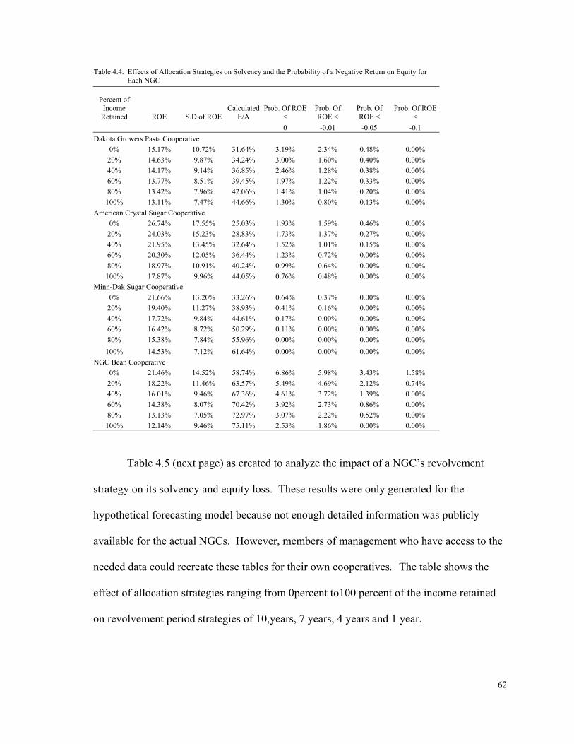
62

Table 4.4. Effects of Allocation Strategies on Solvency and the Probability of a Negative Return on Equity for Each NGC

Percent of Income

Retained ROE S.D of ROE Calculated

E/A Prob. Of ROE

< Prob. Of ROE <

Prob. Of ROE <

Prob. Of ROE <

0 -0.01 -0.05 -0.1 Dakota Growers Pasta Cooperative

0% 15.17% 10.72% 31.64% 3.19% 2.34% 0.48% 0.00% 20% 14.63% 9.87% 34.24% 3.00% 1.60% 0.40% 0.00% 40% 14.17% 9.14% 36.85% 2.46% 1.28% 0.38% 0.00% 60% 13.77% 8.51% 39.45% 1.97% 1.22% 0.33% 0.00% 80% 13.42% 7.96% 42.06% 1.41% 1.04% 0.20% 0.00% 100% 13.11% 7.47% 44.66% 1.30% 0.80% 0.13% 0.00%

American Crystal Sugar Cooperative 0% 26.74% 17.55% 25.03% 1.93% 1.59% 0.46% 0.00%

20% 24.03% 15.23% 28.83% 1.73% 1.37% 0.27% 0.00% 40% 21.95% 13.45% 32.64% 1.52% 1.01% 0.15% 0.00% 60% 20.30% 12.05% 36.44% 1.23% 0.72% 0.00% 0.00% 80% 18.97% 10.91% 40.24% 0.99% 0.64% 0.00% 0.00% 100% 17.87% 9.96% 44.05% 0.76% 0.48% 0.00% 0.00%

Minn-Dak Sugar Cooperative 0% 21.66% 13.20% 33.26% 0.64% 0.37% 0.00% 0.00%

20% 19.40% 11.27% 38.93% 0.41% 0.16% 0.00% 0.00% 40% 17.72% 9.84% 44.61% 0.17% 0.00% 0.00% 0.00% 60% 16.42% 8.72% 50.29% 0.11% 0.00% 0.00% 0.00% 80% 15.38% 7.84% 55.96% 0.00% 0.00% 0.00% 0.00% 100% 14.53% 7.12% 61.64% 0.00% 0.00% 0.00% 0.00%

NGC Bean Cooperative 0% 21.46% 14.52% 58.74% 6.86% 5.98% 3.43% 1.58%

20% 18.22% 11.46% 63.57% 5.49% 4.69% 2.12% 0.74% 40% 16.01% 9.46% 67.36% 4.61% 3.72% 1.39% 0.00% 60% 14.38% 8.07% 70.42% 3.92% 2.73% 0.86% 0.00% 80% 13.13% 7.05% 72.97% 3.07% 2.22% 0.52% 0.00% 100% 12.14% 9.46% 75.11% 2.53% 1.86% 0.00% 0.00%

Table 4.5 (next page) as created to analyze the impact of a NGC’s revolvement

strategy on its solvency and equity loss. These results were only generated for the

hypothetical forecasting model because not enough detailed information was publicly

available for the actual NGCs. However, members of management who have access to the

needed data could recreate these tables for their own cooperatives. The table shows the

effect of allocation strategies ranging from 0percent to100 percent of the income retained

on revolvement period strategies of 10,years, 7 years, 4 years and 1 year.

63

Table 4.5. Effects of Revolvement Cycle Length Changes on the Solvency and Probability of Equity Loss for NGC Bean Cooperative

Percent of Income

Retained ROE S.D. of ROE Projected

Actual E/A Prob. of ROE<

Prob. of ROE<

Prob. of ROE<

Prob. of ROE<

0.00% -1.00% -5.00% -10.00% 10 Yr. Revolvement strategy

0% 21.46% 14.52% 58.74% 6.86% 5.98% 3.43% 1.58% 20% 17.96% 11.19% 63.94% 5.35% 4.57% 2.05% 0.64% 40% 15.72% 9.25% 67.87% 4.49% 3.52% 1.27% 0.31% 60% 14.11% 7.92% 70.97% 3.78% 2.87% 0.80% 0.17% 80% 12.87% 6.94% 73.50% 3.23% 2.27% 0.51% 0.00% 100% 11.89% 9.25% 75.62% 2.83% 1.87% 0.35% 0.00%

7Yr. Revolvement Strategy 0% 21.46% 14.52% 58.74% 6.86% 5.98% 3.43% 1.58%

20% 18.22% 11.46% 63.57% 5.49% 4.69% 2.12% 0.74% 40% 16.01% 9.46% 67.36% 4.61% 3.72% 1.39% 0.00% 60% 14.38% 8.07% 70.42% 3.92% 2.73% 0.86% 0.00% 80% 13.13% 7.05% 72.97% 3.07% 2.22% 0.52% 0.00% 100% 12.14% 9.46% 75.11% 2.53% 1.86% 0.00% 0.00%

4 yr. Revolvement Strategy 0% 21.46% 14.52% 58.74% 6.86% 5.98% 3.43% 1.58%

20% 18.90% 12.02% 62.33% 6.08% 5.16% 2.53% 0.91% 40% 16.99% 10.22% 65.41% 5.09% 3.90% 1.75% 0.00% 60% 15.50% 8.85% 68.09% 3.94% 3.39% 1.16% 0.00% 80% 14.29% 7.77% 70.44% 3.53% 2.68% 0.77% 0.00% 100% 13.29% 10.22% 72.54% 3.02% 2.02% 0.00% 0.00%

1 yr. Revolvement Strategy 0% 21.46% 14.52% 58.74% 6.86% 5.98% 3.43% 1.58%

20% 20.48% 13.23% 59.75% 6.00% 5.18% 2.69% 1.08% 40% 19.69% 12.29% 60.72% 5.33% 4.55% 2.18% 0.76% 60% 18.97% 11.44% 61.64% 4.81% 4.08% 1.81% 0.60% 80% 18.31% 10.67% 62.53% 4.18% 3.53% 1.46% 0.42% 100% 17.71% 12.29% 63.38% 3.76% 2.97% 1.18% 0.28%

The data from Table 4.5 show that, as NGC Bean Cooperative lowers its

revolvement period, ROE and standard deviation of ROE increase while their solvency

ratio decreases. Also, as the revolvement period is shortened, the probability of negative

returns to equity slightly increases. These results show that decreasing revolvement

lengths and decreasing retained income produce similar effects on the solvency positions of

NGCs. This finding is expected because shortening revolvement periods reduces the

reserves of qualified allocations retained (QAR) in much the same way as retaining lower

percentages of income. Both will increase the solvency of the NGC and lower its

probability of equity loss.

64

Validation of Results Using a Value at Risk Extension

Value at Risk (VaR) is receiving considerable attention in the finance literature for

its use in reporting the risks of derivatives (Hendricks, 1996). VaR measures are used to

estimate the probability of a portfolio of assets losing more than a specified amount over a

specified period of time. These losses result from adverse movements in the underlying

market factors of the portfolio (Manfredo and Leuthold, 2000). For example, a VaR

measure of 1 million at a 95 percent confidence level implies that overall portfolio losses

will not exceed 1 million more than 5 percent of the time over a given holding period.

One advantage of VaR relative to other risk measures is its focus on downside risk.

Consequently, VaR has gained attention for being an intuitive measure of risk and for its

ability to capture risks of many different assets into a single concise number. VaR is also

being suggested for firm-level risk management. VaR could be beneficial to management

in making decisions such as how to hedge raw material costs, how to management cash

flows, as well as portfolio selections and allocation decisions. Jorion (1996) defines VaR

as

ασWVaR 0= , (4.1)

where

Wo = initial investment

σ = standard deviation of the investment of the observed period of time,

α = critical value corresponding with one minus the confidence interval such that a

95 percent confidence interval will cause an α value of 1.645 percent and a 99

percent confidence interval will cause an α value of 2.326 (Mason et al., 1994).

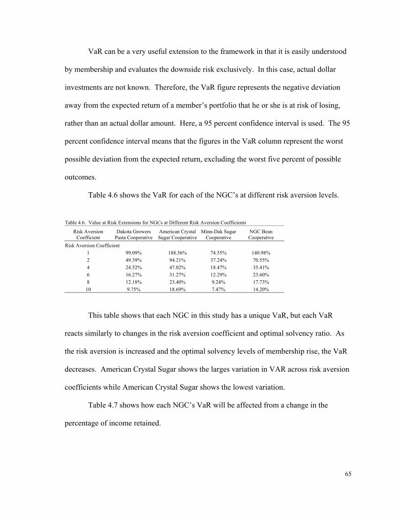
65

VaR can be a very useful extension to the framework in that it is easily understood

by membership and evaluates the downside risk exclusively. In this case, actual dollar

investments are not known. Therefore, the VaR figure represents the negative deviation

away from the expected return of a member’s portfolio that he or she is at risk of losing,

rather than an actual dollar amount. Here, a 95 percent confidence interval is used. The 95

percent confidence interval means that the figures in the VaR column represent the worst

possible deviation from the expected return, excluding the worst five percent of possible

outcomes.

Table 4.6 shows the VaR for each of the NGC’s at different risk aversion levels.

Table 4.6. Value at Risk Extensions for NGCs at Different Risk Aversion Coefficients

Risk Aversion Coefficient

Dakota Growers Pasta Cooperative

American Crystal Sugar Cooperative

Minn-Dak Sugar Cooperative

NGC Bean Cooperative

Risk Aversion Coefficient 1 99.09% 188.56% 74.55% 140.98% 2 49.39% 94.21% 37.24% 70.55% 4 24.52% 47.02% 18.47% 35.41% 6 16.27% 31.27% 12.29% 23.60% 8 12.18% 23.40% 9.24% 17.73% 10 9.75% 18.69% 7.47% 14.20%

This table shows that each NGC in this study has a unique VaR, but each VaR

reacts similarly to changes in the risk aversion coefficient and optimal solvency ratio. As

the risk aversion is increased and the optimal solvency levels of membership rise, the VaR

decreases. American Crystal Sugar shows the larges variation in VAR across risk aversion

coefficients while American Crystal Sugar shows the lowest variation.

Table 4.7 shows how each NGC’s VaR will be affected from a change in the

percentage of income retained.

66

Table 4.7. Value at Risk Extension for NGCs at Different Income Allocation Percentages

Percent of Income Retained

Dakota Growers Pasta Cooperative

American Crystal Sugar Cooperative

Minn-Dak Sugar Cooperative

NGC Bean Cooperative

0% 14.03% 23.01% 17.24% 23.53% 20% 12.91% 19.89% 14.75% 18.56% 40% 11.87% 17.56% 12.89% 15.33% 60% 11.07% 15.74% 11.45% 13.08% 80% 10.38% 14.27% 10.26% 11.83%

100% 9.77% 13.06% 9.37% 11.43%

From looking at the results in Table 4.7, it is apparent that retaining greater

percentages of earning will lower the percentage of expected returns that a member is

capable of losing at a 95 percent confidence interval. It is interesting to note that, although

Minn-Dak has a much greater variance of RA than American Crystal Sugar, it has a lower

VaR. This finding points to the fact that a large portion of Minn-Dak’s variance of RA was

from large positive deviations away from the mean that is not measured as risk in VaR

analysis.

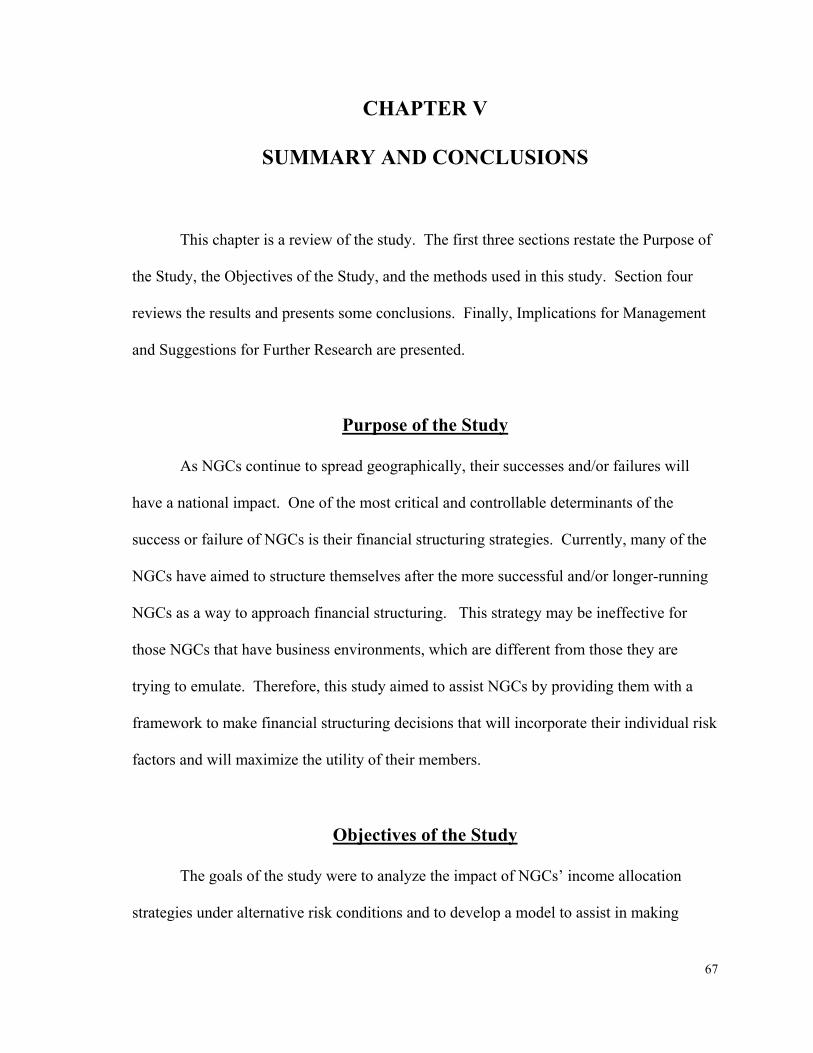
67

CHAPTER V

SUMMARY AND CONCLUSIONS

This chapter is a review of the study. The first three sections restate the Purpose of

the Study, the Objectives of the Study, and the methods used in this study. Section four

reviews the results and presents some conclusions. Finally, Implications for Management

and Suggestions for Further Research are presented.

Purpose of the Study

As NGCs continue to spread geographically, their successes and/or failures will

have a national impact. One of the most critical and controllable determinants of the

success or failure of NGCs is their financial structuring strategies. Currently, many of the

NGCs have aimed to structure themselves after the more successful and/or longer-running

NGCs as a way to approach financial structuring. This strategy may be ineffective for

those NGCs that have business environments, which are different from those they are

trying to emulate. Therefore, this study aimed to assist NGCs by providing them with a

framework to make financial structuring decisions that will incorporate their individual risk

factors and will maximize the utility of their members.

Objectives of the Study

The goals of the study were to analyze the impact of NGCs’ income allocation

strategies under alternative risk conditions and to develop a model to assist in making

68

allocation decisions that will better manage their risk. To reach this goal, the study

observed the current financial strategies used in NGCs by gathering information on those

NGCs that have made their financial statements publicly available. Next, the study

developed a stochastic simulation model that explicitly incorporates input and output price

risks and uncertainty in demand. Then, the study used the optimal solvency model to show

how allocation decisions based on optimal solvency can be used to reduce the probability

of equity loss.

Methods Used in the Study

This study used an expected utility framework to evaluate the optimal income

allocation strategies of NGCs. The model viewed member utility as a function of the mean

and variance of the NGC’s return on equity. The model calculated return on equity as a

factor of the firm’s leverage decision and its mean and variance of return on assets. The

income allocation decisions of NGCs were included in the calculation of the expected

return on assets and the variance of return on assets. Once the return on assets was

quantified, it was substituted in the members’ utility model. This model was then derived

with respect to the NGC’s leverage to find the optimal leverage and solvency for each of

the NGCs. Next, allocation strategies and equity revolvement cycle lengths were evaluated

at the optimal leverage and solvency ratios of each of the NGCs. This evaluation was done

using the stochastic simulation model developed using Excel and At Risk software to

model probability distributions. Also, an analysis was conducted to find the probability of

equity loss for various levels of income allocation and lengths of income revolvement

cycles.

69

Results and Conclusions

This section reviews the results and analysis contained in Chapter IV. First, the

empirically determined solvency ratios and sensitivity analysis are reviewed. Second, the

probability of negative rates of return on equity is discussed. Third, effects of allocation

strategies are examined. Finally, the effects of changes in equity revolvement lengths are

considered.

Empirically Determined Solvency Ratios and Sensitivity Analysis for NGCs (Table 4.2)

Results from Table 4.2 show that each NGC in the study has a different optimal

solvency target. This finding points to the need for each NGC to be evaluated individually,

rather than having one evaluation of a group of NGCs. Although each of the NGCs require

different levels of solvency to maximize member utility, they all react similarly to changes

in the risk aversion coefficient of members. As shown in Figures 5.1 and 5.2, as the

members’ risk aversion is increased, optimal solvency ratios increase while expected

returns fall.

The results displayed in Figures 5.1 and 5.2 (next page) show that, as a NGC’s

membership is more averse to risk, its will be willing to forfeit some of its expected returns

for a decrease in risk. The members are able to decrease their risk by increasing the

solvency of the NGCs. This increasing of the NGC’s solvency position spreads the

cooperative’s net income over a larger equity pool that will lower the return to equity.

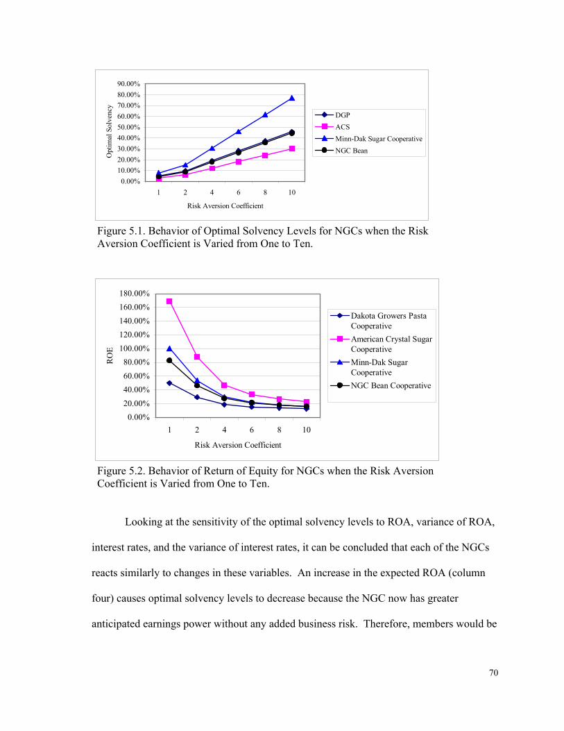
70

0.00%10.00%20.00%30.00%40.00%50.00%60.00%70.00%80.00%90.00%

1 2 4 6 8 10

Risk Aversion Coefficient

Opt

imal

Sol

venc

yDGPACSMinn-Dak Sugar CooperativeNGC Bean

Figure 5.1. Behavior of Optimal Solvency Levels for NGCs when the Risk Aversion Coefficient is Varied from One to Ten.

0.00%20.00%40.00%60.00%80.00%

100.00%120.00%140.00%160.00%180.00%

1 2 4 6 8 10

Risk Aversion Coefficient

RO

E

Dakota Growers PastaCooperativeAmerican Crystal SugarCooperativeMinn-Dak SugarCooperativeNGC Bean Cooperative

Figure 5.2. Behavior of Return of Equity for NGCs when the Risk Aversion Coefficient is Varied from One to Ten.

Looking at the sensitivity of the optimal solvency levels to ROA, variance of ROA,

interest rates, and the variance of interest rates, it can be concluded that each of the NGCs

reacts similarly to changes in these variables. An increase in the expected ROA (column

four) causes optimal solvency levels to decrease because the NGC now has greater

anticipated earnings power without any added business risk. Therefore, members would be

71

willing to take on some added financial risk through debt leveraging to further increase

their expected returns.

As the variance of expected ROA increases (column five), optimal solvency will

increase for each NGC because the NGCs are now subject to greater amounts of business

risk without an increase in the return. Therefore, they would be willing to decrease their

financial risk by reducing their NGC’s debt leveraging. An interest rate decrease (column

six) causes the optimal solvency positions of each of the NGCs to decrease because the

cost of debt financing is reduced so that NGCs can gain greater returns from debt

leveraging with an interest rate drop.

As interest rate variance is increased (column seven), optimal solvency positions of

each of the NGCs will increase because greater uncertainty in interest rates causes greater

financial risk in the NGC. Now, the added returns of debt leveraging are becoming offset

by increased risks. Therefore, members will prefer to use less debt financing, causing the

solvency positions of the NGCs to rise.

NGC management can draw two important conclusions from these data. The first is

that memberships’ risk aversion matters. Therefore, it is important to have a feel for the

risk and return expectations of your members. This information may be gathered through a

general survey designed to weigh members’ risk tolerance. The second is that optimal

solvency is highly sensitive to changes in ROA. When business is good, optimal solvency

levels are going to be low. Therefore, there will be pressure from membership to return

more income and retain less. However, it is important to recognize where the NGC is at in

terms of its business cycle. If the management predicts a downward trend in ROA, it

should plan for the possibility that solvency levels could increase beyond the NGC’s

72

reserves. This scenario would cause the management to reduce the percentage of income

returned at a time when the net income is already lower than in previous years.

Probability of Negative Rate of Return on Equity for NGC (Table 4.3)

In Table 4.3, the Risk Aversion Coefficient, ROA, and Optimal E/A columns are

the same as those seen in Table 4.2. The addition of the standard deviation of ROE column

(column three) allows the managers to see the changes in risk that are results of solvency

changes.

0.00%

20.00%

40.00%

60.00%

80.00%

100.00%

120.00%

140.00%

1 2 4 6 8 10

Risk Aversion Coefficents

Stan

dard

Dev

.of R

OE

Dakota Growers PastaCooperative

American CrystalSugar Cooperative

Minn-Dak SugarCooperative

NGC BeanCooperative

Figure 5.3. The Changes in the Standard Deviation of ROE for NGCs as the Risk Aversion Coefficient is Varied from One to Ten.

Examination of Figure 5.3 reveals that each of the NGCs faces different levels of

risk. Also, each NGC will respond differently to solvency changes resulting from different

levels of risk aversion. American Crystal Sugar and Minn-Dak Cooperative show the

largest responsiveness of standard deviation to changes in risk aversion coefficients while

Dakota Growers Pasta shows the smallest change. Comparing figures 5.1 and 5.3 shows

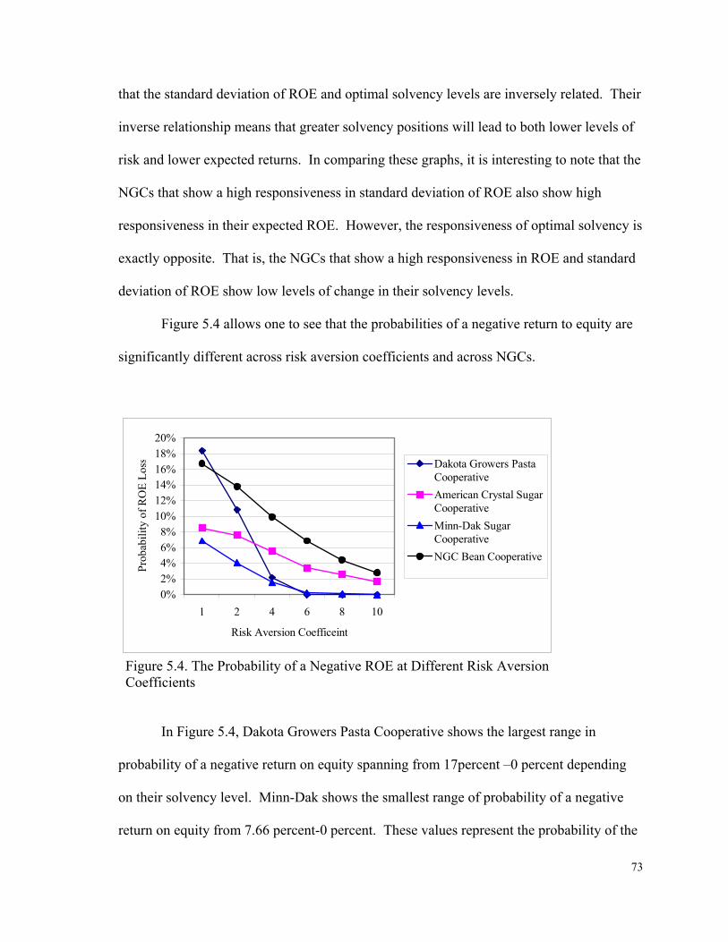
73

that the standard deviation of ROE and optimal solvency levels are inversely related. Their

inverse relationship means that greater solvency positions will lead to both lower levels of

risk and lower expected returns. In comparing these graphs, it is interesting to note that the

NGCs that show a high responsiveness in standard deviation of ROE also show high

responsiveness in their expected ROE. However, the responsiveness of optimal solvency is

exactly opposite. That is, the NGCs that show a high responsiveness in ROE and standard

deviation of ROE show low levels of change in their solvency levels.

Figure 5.4 allows one to see that the probabilities of a negative return to equity are

significantly different across risk aversion coefficients and across NGCs.

0%2%4%6%8%

10%12%14%16%18%20%

1 2 4 6 8 10

Risk Aversion Coefficeint

Prob

abili

ty o

f RO

E Lo

ss Dakota Growers PastaCooperativeAmerican Crystal SugarCooperativeMinn-Dak SugarCooperativeNGC Bean Cooperative

Figure 5.4. The Probability of a Negative ROE at Different Risk Aversion Coefficients

In Figure 5.4, Dakota Growers Pasta Cooperative shows the largest range in

probability of a negative return on equity spanning from 17percent –0 percent depending

on their solvency level. Minn-Dak shows the smallest range of probability of a negative

return on equity from 7.66 percent-0 percent. These values represent the probability of the

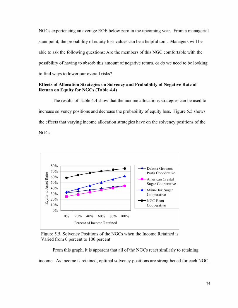
74

NGCs experiencing an average ROE below zero in the upcoming year. From a managerial

standpoint, the probability of equity loss values can be a helpful tool. Managers will be

able to ask the following questions: Are the members of this NGC comfortable with the

possibility of having to absorb this amount of negative return, or do we need to be looking

to find ways to lower our overall risks?

Effects of Allocation Strategies on Solvency and Probability of Negative Rate of Return on Equity for NGCs (Table 4.4)

The results of Table 4.4 show that the income allocations strategies can be used to

increase solvency positions and decrease the probability of equity loss. Figure 5.5 shows

the effects that varying income allocation strategies have on the solvency positions of the

NGCs.

0%10%20%30%40%50%60%70%80%

0% 20% 40% 60% 80% 100%

Percent of Income Retained

Equi

ty to

Ass

et R

atio

Dakota GrowersPasta CooperativeAmerican CrystalSugar CooperativeMinn-Dak SugarCooperativeNGC BeanCooperative

Figure 5.5. Solvency Positions of the NGCs when the Income Retained is Varied from 0 percent to 100 percent.

From this graph, it is apparent that all of the NGCs react similarly to retaining

income. As income is retained, optimal solvency positions are strengthened for each NGC.

75

Also, Figure 5.6 shows that, as more income is retained and the solvency increases, the

probability of a negative return to equity decreases.

0.00%1.00%2.00%3.00%4.00%5.00%6.00%7.00%8.00%

0% 20% 40% 60% 80% 100%

Percent of Income Retained

Prob

abili

ty o

f a N

egat

ive

RO

E

Dakota Growers PastaCooperativeAmerican Crystal SugarCooperativeMinn-Dak SugarCooperativeNGC Bean Cooperative

Figure 5.6. The Probability of Equity Loss for NGCs at Different Allocation Percentages

These graphs show that NGCs can effectively use allocation decisions based on optimal

solvency targets to reduce their overall risk.

Effects of Changes in the Length of Revolvement Cycles on Solvency and the Probability of Equity Loss (Table 4.5)

Up to this point, the study has evaluated the results of changes to risk aversion

levels of members and income allocation percentages. In Table 4.5, revolvement cycle

length changes are evaluated as a way to manage risk. Figure 5.7 (next page) shows the

effects of revolvement length changes on the solvency position of NGC Bean Cooperative

at different income retention strategies.

Figure 5.7 (next page) shows that decreasing the length of the revolvement cycle

will result in lower levels of optimal solvency as long as there is some income being

76

retained. Also, the revolvement length strategy is less effective for NGCs that retain low

amounts of income.

0.5

0.55

0.6

0.65

0.7

0.75

0.8

1 yr. 4 yr. 7Yr. 10 Yr.

Revolvement Length

Opt

imal

Sol

venc

y 0% Retained20% Retained40% Retained60% Retained80% Retained100% Retained

Figure 5.7. Solvency Level of NGC Bean Cooperative at Different Income Allocation Percentages when the Revolvement of Retained Income is Varied from One to Ten Years.

It makes sense that retaining income more quickly will lead to lower levels of

solvency. An NGC’s solvency will decrease because it is in a level growth stage and will

build equity reserves until it enters its first year of repayment. After that point, the NGC

will be offsetting its retained income with prior year’s retained income that is being

revolved out of the cooperative. When revolvement strategies are lengthened, it gives the

NGC additional time to build up reserves before it must revolve them back. It is also

makes sense that revolvement length changes will be more effective for NGCs that retain

greater amounts of income. The greater the amount retained, the larger the equity reserve

will be and the larger the revolvement payments will be. With larger reserves and larger

77

payments from the reserves, revolvement length changes will have a greater impact on the

overall solvency of the NGC.

A drawback of this strategy is that lengthening revolvement periods will come with

strong resistance from the NGC’s members unless the reasoning is clearly and thoroughly

explained to them. The resistance is because members value knowing when their retained

earnings will be revolved as they have already figured the payments into their cash flow

statements of their production operations. Also, because revolved income is distributed

back without a return, the time value of money will cause the returns to have a lower net

present value as revolvement periods increase in years. This can make changes in

revolvement cycle lengths an unsuccessful strategy from the standpoint of membership

utility.

The Effects of Changes in Risk Aversion on Value at Risk (Table 4.6)

Figure 5.8 (next page) graphically demonstrates the data in Table 4.6. This figure

shows that, as risk aversion is increased and the solvency levels of membership rise, the

VaR decreases at a decreasing rate.

It is logical that greater risk aversion would lead to a lower VaR, as VaR is a

measure of overall risk. These results could also prove to be a valuable tool for managers

and members. For many NGCs, it will be quite difficult to determine the membership’s

average risk aversion. However, managers and members may be able to agree on a

combination of expected return and VaR that they are comfortable with. From there they

could determine the allocation strategy that best meet these objectives.

78

0.00%20.00%40.00%60.00%80.00%

100.00%120.00%140.00%160.00%180.00%200.00%

1 2 4 6 8 10

Risk Aversion Coefficients

Val

ue a

t Ris

kDakota Growers PastaCooperative

American CrystalSugar Cooperative

Minn-Dak SugarCooperative

NGC BeanCooperative

Figure 5.8 Value at risk of the NGCs when the Risk Aversion Coefficient is Varied from One to Ten.

Effects of Changes in Allocation Strategies on Value at Risk (Table 4.7)

Figure 5.9 graphically demonstrates the data in Table 4.7. This figure shows the

change in VAR for the NGCs at different allocation strategies.

0%

5%

10%

15%

20%

25%

0% 20% 40% 60% 80% 100%

Percent of Income Retained

Val

ue-a

t-Ris

k

Dakota GrowersPasta Cooperative

American CrystalSugar Cooperative

Minn-Dak SugarCooperative

NGC BeanCooperative

Figure 5.9. The Change in the Value at Risk for the NGCs when the Income Retained is Varied from 0 percent to 100 percent for NGCs at Different Allocation Strategies

79

For NGCs, having a high responsiveness of solvency to changes in income

allocation strategies will result in allocation strategies being a more effective risk

management tool. In examining Figure 5.9, Dakota Growers has the smallest change in

VaR as a result of income retention changes. This finding is consistent with its small

change in solvency position. Also, NGC Bean has the largest change in VaR while having

the second largest change in equity to assets. This finding shows that the effectiveness of

allocation strategies is going to depend strongly on the NGC’s current financial position.

Having large amounts of long-term debt relative to expected ROA will weaken the ability

of an NGC to change its solvency position.

Implications for Management

The following list details a number ways in which manages can benefit from this

study.

1) Managers and directors of NGCs can use the models developed in this study to

arrive at an allocation strategy that is tailored to their individual cooperative.

2) By gathering historical information on their cooperative, Managers will be able to

view their NGC’s probability of equity loss and value at risk for different income

allocation percentages. Managers can then use this information to survey members

and get a more accurate feel for their risk tolerance. This process will assist in

making allocations decisions.

3) For NGCs with limited history, the deterministic forecasting model can be used to

generate the needed financial information to determine the NGC’s optimal solvency

targets, probability of equity loss, and value at risk at different risk aversion levels.

80

Suggestions for Further Research

The following is a list of suggestions on ways this work could be furthered to benefit those

interested in the long-term viability of NGC’s.

1) From looking at Table 4.2 and 4.3, it is apparent that the risk aversion of members

plays a significant role in determining the optimal solvency of members of NGCs.

For this reason, more research is needed accurately determine the risk aversion of

NGC members and the optimal solvency of NGC. This research, however, would

need to be done on a cooperative-by-cooperative basis.

2) Further research could use this forecasting model on other forms of NGCs,

including, but not limited to ethanol cooperatives, livestock cooperatives, fruit and

vegetable growers cooperatives and cotton cooperatives.

3) This study was limited in the amount of detailed information that was available to

use in the forecasting model. Having access to such information would make it

possible to create more accurate and detailed forecasts and suggestions for actual

NGCs.

4) This study examined the income allocation decision’s effect on member utility and

probability of equity loss. This model could be easily adapted to provide insight as

to the effects of other financial indicators representing efficiency, financial

flexibility, and profitability.

5) This modeling only looks at the strategies of allocating income in the form of

qualified retained earning or cash allocations. However, NGCs also have the option

of using non-qualified allocations and unallocated reserves. An advancement of

81

this study could be to model the effectiveness of these allocation strategies in

addition to the strategies examined in this study.

6) This model is also evaluating the allocation strategies assuming a level growth rate

for the NGCs. Further studies could be conducted to view the impact of allocation

strategies on NGCs that are in growth or decreasing sales trends. Also, the impact

of operating cycles in a NGC’s industry could be examined.

82

REFRENCES

American Crystal Sugar Cooperative’s Website. www.crystalsugar.com. Created N.D.

Reviewed December 2001. American Crystal Sugar Cooperative’s Annual 10-K Securities and Exchange Filings from

Years 1994-2000. http://www.edgar-online.com/fts/search.asp Created N.D. Reviewed March 2001.

Barry, Peter J., and Lindon J. Robison. “Portfolio Theory and Financial Structure: An

Application of Equilibrium Analysis.” Agricultural Finance Review. 47 1987 pp142-151.

Barry, Peter J., Paul N. Ellinger, John A. Hopkin, and C.B. Baker. Financial Management

in Agriculture Fifth Edition. Interstate Publisher Inc. Danville, Ill. 1995 pp157.

Bielik, Michelle, and Brian Oleson. Agri-Food Research and Development Initiative (ARDI) Web page. University of Manitoba, Department of Agricultural Economics & Farm Management. http://www.umanitoba.ca/afs/agriceconomics/ardi/ Created 1996. Reviewed August 2000.

Black, Roy J., Barry J. Barnett and Hu Yingyao. “Cooperatives in Capital Markets: The Case of Minnesota-Dakota Sugar Cooperatives,” American Journal of Agricultural Economics. 81 1999 pp 1240-1246.

Brigham, Eugene F. Fundamentals of Financial Management. Harcourt Brace College Publishers. Orlando, Fl. 1995 pp 423-489.

Campbell, Dan. “Wave Maker: A Conversation With Mark Hanson, A Key

Player In Minnesota’s New Wave Co-op Movement.” Farmer Cooperatives. 62 October1995 pp 18-22.

Collins, Robert A. “Expected Utility, Debt-Equity Structure and Risk Balancing.”

American Journal of Agricultural Economics. 67 1985 pp 627-629.

Cook, Michael C., Brice Ratchford, and Brian Griffith. “How Cooperatives are Taxed.” http://www.muextension.missouri.edu/xplor/agguides/agecon/g00903.htm. Created N.D. Reviewed March 1995.

Coon, Randal C., and F. Larry Leistritz “Economic Contribution North Dakota

Cooperatives Make to the State Economy.” North Dakota State University Department of Agribusiness and Applied Economics Staff Paper 01002. March, 2001.pp.2-3.

Dakota Growers Pasta’s Annual 10-K Securities and Exchange Filings from Years 1994-

2000. http://www.edgar-online.com/fts/search.asp Created N.D. Reviewed March 2001.

83

Diaz-Hermelo, Francisco, Allan Gray, and Edward Smith. “Modeling Member Responses

to the Farmer Owned Cooperative’s Alternative Capital Management Strategies.”AAEA Annual Meeting Chicago, Ill. August 5-8 2001.

Economic Development Background Memorandum. Prepared by the North Dakota Legislative Council Staff for the Commerce and Labor Committee. North Dakota Legislative Council web site http://www.state.nd.us/lr/dtsearch/ Created July 1999. Reviewed March 2000.

Escalante, Cesar L., and Peter J. Barry. “Farm Level Evidence on the Risk Balancing

Hypothesis from Illinois Grain Farms.” AEAA Annual Meeting Chicago, Ill. August 5-8 2001.

Featherstone, Allen M., Charles B. Moss, Timothy G. Baker, and Paul V. Preckel. “The Theoretical Effects of Farm Policies on Optimal Leverage and the Probability of Equity Losses.” American Journal of Agricultural Economics. 70 1988 pp 573-579.

Gabriel, Stephen C., and C.B. Baker. “Concepts of Business and Financial Risk.” American Journal of Agricultural Economics. 62 1980 pp 560-564.

Hendricks, Darryll. “Evaluation of Value at Risk Models Using Historical Data” Federal Reserve Bank of New York Economic Policy Review. 2 1996 pp 39-69.

Holmes, Mary, Norman Walzer, and Christopher D. Merrett. New Generation Cooperatives: Case Studies. Illinois Institute for Rural Affairs. Macomb, IL August 2001.

Internal Revenue Service. “How to Depreciate Property.” Publication 946. 2001 pp 60. Jensen, Farrell E., and Larry N. Langemeier. “Optimal Leverage with Risk Aversion:

Empirical Evidence.” Agricultural Finance Review. 56 1996 pp 85-97. Jorion, P., F.J. Maude, and W. Perraudin. “Measuring the Risk in Value at Risk.” Financial

Analysts Journal. 52 1996 pp 47-56.

Kelly, Christopher R. “New Generation Farmer Cooperatives.” American Agricultural Law Update. 17 2000 pp 4-7.

Knapp, Joseph. The Advance of American Cooperative Enterprise. Interstate Printers and Publishers Danville, Ill. 1973 pp .

Leistritz, Larry F., and Randall S. Sell. “Agricultural Processing in North

Dakota: Socioeconomic Impacts.” North Dakota State University Agricultural Economics Department Report No. 437. Fargo, ND 2000.

84

Longstaff, Francis A. “How Much Can Marketability Affect Security Values?” Journal of

Finance. 50 1995 pp 1767-1774. Manfredo, Mark R., and Raymond M. Leuthold. “Value-at-Risk Analysis: A Review and

the Potential for Agricultural Applications.” Review of Agricultural Economics. 21 2000 pp 99-111.

Mason, Robert D., Douglas A. Lind, and William G. Marchal, Statistics An Introduction Forth Edition, Duxbury Press Boston, MA 1994 pp 381.

Mather, Warren, Katherine C. DeVille, and Celestine C. Adams. “Cooperative Historical Statistics.” Cooperative Information Report 1 Section 26 USDA Cooperative Service. Washington, D.C. April 1998.

Merrett, Christopher, Mary Holmes, and Jennifer Waner. Directory of

New Generation Cooperatives. Illinois Institute for Rural Affairs. Macomb, IL September 1999.

Meyers, S.S. “The Capital Structure Puzzle.” Journal of Finance. 1984, pp 575-592. Miller, Merton H., and Franco Modigliani. “Dividend Policy and Valuation of Shares.”

Journal of Business. 34 1961 pp 411-433.

Minn-Dak Sugar Cooperative’s Annual 10-K Securities and Exchange Filings from Years 1994-2000. http://www.edgar-online.com/fts/search.asp Created N.D. Reviewed March 2001.

Nelson, William. Director, Quinton Burdick Center for Cooperatives. Personal Interview.

December 2001.

Olson, Frane. “Should I Join a Processing Cooperative?” North Dakota State University Extension Service Report EB-67. Fargo, ND 1999.

Parcell, Joseph L., Allen M Featherstone, and David G. Barton. “Capital Structure Under Stochastic Interest Rates: Agricultural Cooperatives.” Agricultural Finance Review. 58 1990 pp 49-61.

Poray, Michael C. and Roger Ginder. “Large Scale Closed Contract Cooperative

Swine Production Under Uncertainty.” Presented at the 1997 AAEA National Conference in Toronto, ON. July 28-29,1997.

Richard, Mary Jo. Partner, Eide Bailly LLP. Personal Interview. August 2001.

85

Stefanson, Brenda, Murry Fultan, and Andrea Harris, “New Generation Co-operatives Rebuilding Rural Economies.” Centre for the Study for Co-operatives, University of Saskatchewan. Saskatoon, Saskatchewan. 1995.

Stefanson, Brenda and Murry Fultan. “New Generation Co-operatives Responding to Changes in Agriculture.” Centre for the Study for Co-operatives, University of Saskatchewan. Saskatoon, Saskatchewan.1997.

86

APPENDIX A

PERCENT OF ALL EQUITIES MODEL

In the “percent of all equities” approach to equity management, we still assume that

Pi and Ci are the stochastic variables. The decision variables that management can look at

in this representation are split into two groups. Qac%n, Qar%n, Nqa%n, and Uar%n, are the

various choices of income allocation available to management. These choices are the same

as those in the fixed-year revolvement plan. The new allocation choices are Qaro%n and

Nqao%n. They represent the choices regarding the percentage of cash that will be revolved

out of the member equity accounts. The equity accounts of common stock, paid in capital,

qualified allocations, non-qualified allocations, and unallocated reserves are known.

The representation of the percent of all equities approach changes our original ROA

(equation 3.13) so that ROA is represented as

nnnnnnnn

nnnnnnnn

nnn

Uar%*NIBTQar%*NIBTNqa%*NIBTQar*Qaro%Nqa*Nqao%UarNqaQarPicCsD

DKNIBTROA

+++−−+++++⋅+

= ,

(A.1)

where

NIBTn = net income in the current period before taxes are deducted

Kn = weighted average interest cost of debt

Dn = total debt

Cs n = the balance of common stock for the current period

Pic n = the balance of paid in capital for the current period

87

UAR% n = the percentage of income that is placed in an unallocated reserve account

at the end of the current period

Qarn = the current balance of the qualified allocation redeemed account

Nqan = the current balance of the non-qualified allocations account,

Uarn = the current balance in the unallocated reserve accounts

Qar%n = the percentage of NIBT that is allocated to a qualified allocation account

at the end of the current period

Nqa%n = the percentage of NIBT that is allocated to a non-qualified allocation

account at the end of the current period

Uar%n = the percentage of NIBT that is allocated to an unallocated reserve account

at the end of the current period

Qaro%n = the percentage of NIBT that is redeemed out of the qualified allocation

account at the end of the current period

Nqao%n = the percentage of NIBT that is redeemed out of the non-qualified

allocation account at the end of the current period.

This model assumes that management is using a “percent of all equities” approach

for the redemption of qualified and non-qualified reserve balances. This approach differs

from the fixed-year revolvement approach in that the management and board of directors

will set the percentage of the reserve balances to pay back to members, rather than setting a

fixed-year revolvement schedule. The positive aspect of this plan is that, by allocating only

a percentage of an equity balance rather than a fixed amount, the NGC will have a

buffering mechanism to ensure that equity reserves do not fall too quickly in times of low

income. The drawback is that members would not have a known dollar value being

88

revolved to them that they can use for cash flow planning for their production operation.

This allocation strategy would also make it more difficult for members to put a price on

their stock as future cash payments are uncertain.

89

APPENDIX B

OPTIMAL SOLVNECY CALCULATIOR

Table A.1. Calculation of Optimal Solvency ROA Interest Rates Abbreviation

1 8.00% 7.81% Mean ROA A 2 5.00% 8.30% Mean Interest Rates K 3 6.00% 8.40% Standard Deviation of ROA Sa 4 10.25% 8.70% 5 9.40% 10.00% Standard Deviation of Interest Rates Sk 6 10.14% 8.16% Variance of ROA Va 7 15.00% 7.90% Variance of Interest Rates Vk 8 16.00% 7.60% Correlation C 9 5.00% 8.40% Risk Aversion Coefficient Y

10 9.99% 7.90% Mean 9.48% 8.32% Optimal Solvency (S) St. Dev 3.78% 0.68% Numerator=

Y(Va- (2*C*Sa*Sk+ Va))

Variance 0.1430% 0.0046% Denominator=

R-K+A*K*(Sk-C*Sa)

Correlation Interest Rates Numerator = 0.82% ROA -0.301075591 Denominator= 1.22% S= 66.69% Risk Aversion 5 Coefficient Return on Equity (ROE) A-K*(1-S)*(1/S) ROE= 10.0579% Variance of Return on Equity Var. (ROE)

(Va+Vk-C*Sa*Sk)/S^2

Var ROE= 0.35%

90

APPENDIX C

DESCRIPTION OF NET INCOME BEFORE TAX AND DEBT

From the deterministic model, NIBTn in equation 3.11 can be derived to form the

following equation.

iiiiiiin FcQVcQRdQPNIBIT −⋅−⋅−⋅= , (A.2)

where

Pi = the price of product i

Qi = the quantity of product i that is sold in the current period

Rdi = the percentage royalties and discounts associated with product i

Vci = the variable costs associated with the production of product i

Fci = the fixed costs associated with product i, and

Kn = the weighted average interest rate of total debt in the current period.

In this equation, we assume that Pi and Ci are the stochastic variables. This

modeling captures both the uncertainty in raw material inputs and the price received

for the products. The decision variables that management can observe in this

representation are Qac%n, Qar%n, Nqa%n, and Uar%n, which, again, are the various

choices of income allocation available to management.