an analysis of belief propagation on the turbo decoding ...rusmevic/psfiles/turbo.pdfthe turbo...
TRANSCRIPT

October 20, 2000
An Analysis of Belief Propagation onthe Turbo Decoding Graph with Gaussian Densities
Paat Rusmevichientong and Benjamin Van RoyStanford University
{paatrus,bvr}@stanford.edu

ABSTRACT
Motivated by its success in decoding turbo codes, we provide an analysis of the beliefpropagation algorithm on the turbo decoding graph with Gaussian densities. In this context,we are able to show that, under certain conditions, the algorithm converges and that –somewhat surprisingly – though the density generated by belief propagation may differsignificantly from the desired posterior density, the means of these two densities coincide.
Since computation of posterior distributions is tractable when densities are Gaussian,use of belief propagation in such a setting may appear unwarranted. Indeed, our primarymotivation for studying belief propagation in this context stems from a desire to enhanceour understanding of the algorithm’s dynamics in non-Gaussian setting, and to gain in-sights into its excellent performance in turbo codes. Nevertheless, even when the densitiesare Gaussian, belief propagation may sometimes provide a more efficient alternative totraditional inference methods.
Key words: approximate inference, belief network, belief propagation, Gaussian densities,and turbo decoding.
1

1 Introduction
Probability distributions provide a tool for characterizing beliefs about unobserved quan-tities and relationships among them. As observations are made, beliefs change and poste-rior distributions evolve to reflect improved understanding. Unfortunately, the process ofinference – that of computing posterior distributions – often entails integration over high–dimensional spaces and is typically intractable. One exception arises when densities areGaussian. In this case, posterior distributions – which are also Gaussian – can be computedefficiently and represented compactly in terms of means and covariances.
Another case that admits efficient computation arises when conditional independenciesamong random variables form a convenient pattern. Belief networks and Markov randomfields offer two approaches to characterizing such conditional independencies in terms ofdirected and undirected graphs, respectively. In either case, when the graph is singly con-nected (i.e., when there are no cycles), belief propagation – an efficient inference algorithm– becomes applicable [13, 22].
Many distributions of interest are not Gaussian and do not accommodate singly–connectedgraphs. In such cases, exact inference is typically intractable, and approximations are calledfor. Surprisingly, although belief propagation was developed for singly-connected graphs,it has been shown to deliver impressive performance in many applications involving graphswith cycles. A notable example of this is the turbo decoding algorithm used in turbo codes.
The turbo decoding algorithm is an approximation method that has delivered impressiveperformance in certain coding applications [5, 6]. The inference task originally addressedby the turbo decoding algorithm involves computing a distribution over the underlyingmessage after receiving an encoded transmission across a noisy communication channel.The structure of the encoding scheme – which makes use of “turbo codes” – leads to efficienttransmission rates, but leaves the decoder with the job of solving an intractable inferenceproblem. The turbo decoding algorithm has proven to be an effective approximation methodfor this task. Because its initial development was not supported by mathematical theory,spectacular empirical success was received with surprise, excitement, and intrigue.
It turns out that the turbo decoding algorithm is equivalent to belief propagation. Thisconnection was first noted by Frey and Kschischang [11] and McEliece [20]. In particu-lar, McEliece, MacKay, and Cheng [19] presented an interpretation of the turbo decodingalgorithm as an application of belief propagation in a graph with cycles. Since belief prop-agation was developed for singly–connected graphs, application in the presence of cycles –as is done in turbo decoding – was not supported by pre–existing principles.
With the excitement spawned by success of the turbo decoding algorithm came a reex-amination of iterative decoding algorithms for codes on graphs [31, 32] and message passingalgorithms [12]. Message passing algorithms were proposed decades earlier in the codingliterature and bear similarities with the turbo decoding algorithm. Designed for decoding oflow density parity check codes, message passing algorithms turned out also to correspond tobelief propagation in graphs with cycles. Furthermore, a recent empirical study establishesthat message–passing algorithms share the impressive performance demonstrated by turbodecoding [18, 24].
Indeed, Kschischang and Frey [14, 15] have shown that iterative decoding algorithms,belief propagation, and various message passing algorithms are unified by a single frame-work involving a distributed marginalization algorithm for functions characterized by factor
2
graphs. They also show that many algorithms in artificial intelligence, signal processing,and digital communications, which were each developed independently, fit naturally intothis framework. A similar unifying framework was also proposed in [3].
There are also signs of promise for belief propagation (in graphs with cycles) in inferenceproblems beyond those arising in coding. Positive results have been generated – for example– in empirical case studies motivated by applications in image processing and medical deci-sion making [21]. However, in some case studies, the algorithm fails, and factors influencingperformance are not well–understood. Analytical work has focused on identifying suitableclasses of problems and understanding why their properties foster success.
Recent analyses focusing on the context of coding [17, 23, 25] extend early work byGallager [12] to shed light on the success of turbo decoding and message passing algorithms.In very rough terms, the thrust of this line of research involves establishing that cyclesarising in relevant coding applications are “generally very long” and showing that this allowsbelief propagation to work “almost as well as in singly–connected graphs.” Additional workspecialized to the context of low density parity check codes further strengthens these results[24].
Another line of analytical work has aimed at understanding the behavior of belief prop-agation in general graphs with cycles. As a starting point, several researchers have studiedthe case involving a graph with a single cycle [2, 8, 28]. This case is not useful in its ownright, since exact inference is tractable in the presence of a single cycle. However, thestudy of this case has lead to concise results that enhance our state of understanding. Inparticular, results pertaining to the case of a single cycle include:
1. Belief propagation converges to a unique stationary point.
2. If all random variables are binary–valued, the component–wise maximum likelihoodestimates offered by the resulting approximation concur with true maximum likelihoodvalues.
Unfortunately, the line of analysis employed for the case with a single cycle does not imme-diately extend to graphs with multiple cycles.
In this paper, we study belief propagation from a new angle by analyzing its dynamicsin a restrictive setting where densities are Gaussian. We focus our attention on the casewhere the dependence structure of the random variables is similar to the one that appearedin the original turbo decoding application. The graph that captures this dependency willbe referred to as the turbo decoding graph. In this case, exact inference is tractable anduse of belief propagation is not entirely necessary. Nevertheless, belief propagation maysometimes provide a more efficient method for solving certain inference problems in thiscontext. Our primary motivation for studying the Gaussian case, however, is to provide asetting amenable to a streamlined analysis. A clear understanding here may offer insightsinto behavior of belief propagation in more general settings, and possibly shed light on itssuccess in turbo codes.
Contributions of our analysis include certain concise results concerning use of beliefpropagation when densities are Gaussian:
1. If belief propagation is initialized with Gaussian densities, each iterate is also Gaussian(Lemma 2).
3

2. The associated sequence of covariance matrices converges to a unique stationary point(Theorem 1).
3. Under certain conditions, the sequence of mean vectors also converges to a uniquestationary point (Theorem 2, Proposition 1, 2, 3, 4, and 5).
4. When belief propagation converges, the mean of the resulting approximation coincideswith that of the true posterior density (Theorem 3). (Note that, since the distributionis Gaussian, the mean corresponds to the maximum likelihood value, so this resultparallels an aforementioned result concerning the case of a graph with a single cycleand binary variables.)
While preparing this paper, we became aware of two related initiatives, both involvinganalysis of belief propagation when densities are Gaussian and graphs possess cycles. Weissand Freeman [30] were studying the case of 2-dimensional lattice. Here, they were ableto show that, if belief propagation converges, the mean of the resulting approximationcoincides with that of the true posterior distribution. Weiss and Freeman also derivedequations characterizing dynamics of means and covariance matrices generated by beliefpropagation. At the same time, Frey [10] studied a case involving graphical structures thatgeneralize those employed in turbo decoding. He derived an equation satisfied by stationarypoints and provided an analysis relating convergence of means to the spectral radius of aparticular matrix (we will present and analyze a related matrix in Section 5.2). He alsoconducted an empirical study. Coincidentally, short papers describing the work of Weissand Freeman [29] and Frey [9], as well as one summarizing results in this paper [26], weresimultaneously submitted to the same conference.
The paper is organized as follow. In the next section, we provide our working definitionof the belief propagation algorithm. To lend concreteness to this definition, we present anexample in Section 3 of a situation where belief propagation might be more efficient thantraditional inference methods. In Section 4, we discuss specialization of belief propagationto the Gaussian case. A convergence analysis is then presented in Section 5. In section6, we prove that the mean of the approximation generated by belief propagation coincideswith that of the desired posterior distribution. After presenting some experimental results,we close with a concluding section.
2 Belief Propagation on the Turbo Decoding Graph
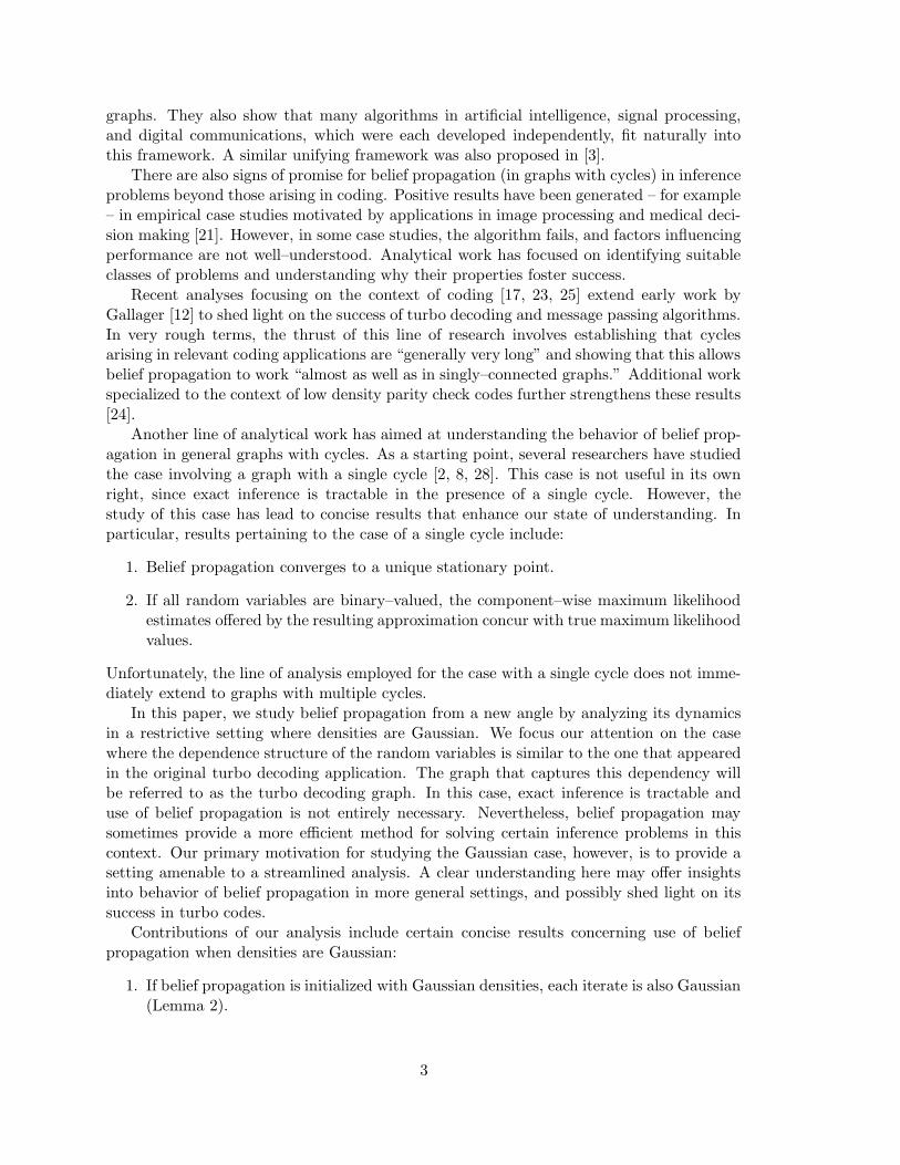
Consider a random variable x that takes on values in <n and has independent components.Let p0 denote the prior density of x. Also, let y1 and y2 be two random variables that areconditionally independent given x. For example, y1 and y2 might represent outcomes oftwo independent transmissions of the signal x over a memoryless communication channel.The turbo decoding graph depicting the dependence among the random variables (both inBayesian network and factor graph representation) is given in Figure 1. Our definition ofbelief propagation will exploit the dependence structure of these random variables.
If y1 and y2 are observed, one might want to infer a posterior density f of x conditionedon y1 and y2. This can be obtained by first computing densities p∗1 and p∗2, where the first
4
X2 X3 XnX1
y21
y
X1 X2 X3 Xn
g1
g2
g3
gn
1f
1y
f2
2y(a) (b)
Figure 1: Turbo Decoding Graph (a) Bayesian network representation, (b) factor graphrepresentation. In (b), the function f1 (resp. f2) corresponds to the conditional density ofy1 (resp. y2) given x. The function gi corresponds to the prior density of xi.
is conditioned on y1 and the second is conditioned on y2. Then,
f = α
(
p∗1p∗2
p0
)
,
where α is a “normalizing operator” defined by
αg =g
∫
g(x)dx,
and multiplication and division are carried out pointwise.Unfortunately, even when p∗1 and p∗2 are known, computation of f can be intractable.
The burden associated with storing and manipulating high–dimensional densities appearsto be the primary obstacle. This motivates the idea of limiting attention to densities thatfactor. In this context, it is convenient to define an operator π that generates a density thatfactors while possessing the same marginals as another density. In particular, this operatoris defined by
(πg)(a) =n∏
i=1
∫
{x∈<n|xi=ai}g(x)dx ∧ dxi,
for any density g and any a ∈ <n, where dx ∧ dxi = dx1 · · · dxi−1dxi+1 · · · dxn. One mightaim at computing πf as a proxy for f . Unfortunately, even this problem can be intractable.Belief propagation can be viewed as an iterative algorithm for approximating πf .
Let operators T1 and T2 be defined by
T1g = α
((
πp∗1g
p0
)
p0
g
)
,
and
T2g = α
((
πgp∗2p0
)
p0
g
)
,
for any density g. Belief propagation is applicable in cases where computation of these two
operations is tractable. The algorithm generates sequences q(k)1 and q
(k)2 according to
q(k+1)1 = T1q
(k)2 and q
(k+1)2 = T2q
(k)1 .
initialized with densities q(0)1 and q
(0)2 that factor. The hope is that α(q
(k)1 q
(k)2 /p0) converges
to a useful approximation of πf .
5
an
n-1b b n
an-1a1 a2
b 1 b 2
Figure 2: An example of a hidden Markov model.
3 An Example
The preceding abstract definition relied on use of operators T1 and T2 as subroutines. Forthe sake of concreteness, we will discuss in this section certain situations where computationof T1 and T2 is tractable. It is in such situations that belief propagation may constitute alegitimate approximation scheme.
We will describe an example in terms of Markov random fields, so let us begin byreviewing the semantics of this graphical modeling framework. A Markov random field isan undirected graph with each node corresponding to a random variable. The arcs conveyinformation about conditional independencies. In particular, if A, B, and C, are mutuallyexclusive sets of nodes and C separates A from B, then the random variables correspondingto A are conditionally independent from those corresponding to B conditioned on thosecorresponding to C. The term separates refers to the fact that every path from a node in Ato a node in B visits at least one node in C.
When a Markov random field is singly connected, belief propagation offers an efficientapproach to inference. In particular, when some of the variables are observed, a poste-rior distribution over the remaining variables, and furthermore, marginal distributions overindividual variables, can be efficiently computed.
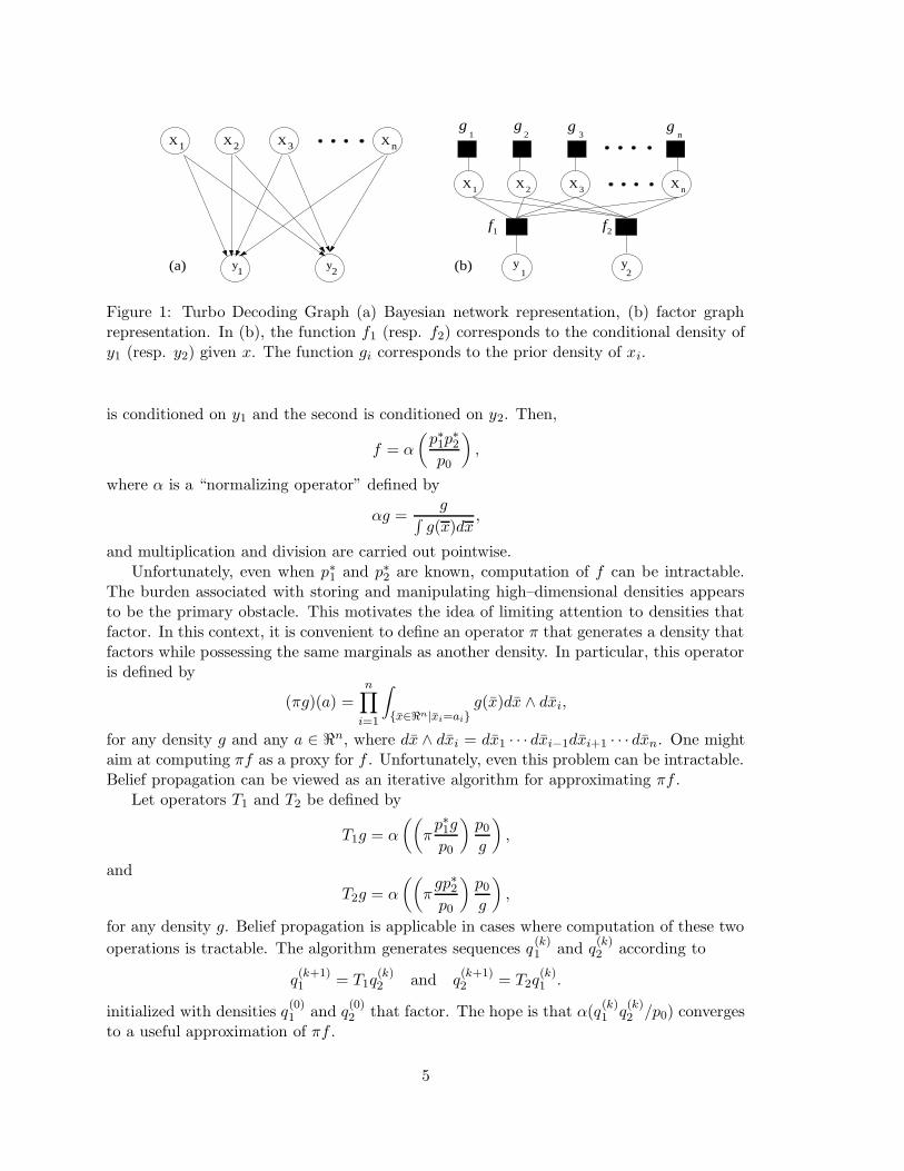
One common class of Markov random fields that accommodates efficient inference is theclass of hidden Markov models. Figure 2 depicts the Markov random field associated with asimple hidden Markov model. The nodes are labeled with corresponding random variables.It is easy to see that the graph is singly connected, and the common inference problemof computing a posterior distribution over a1, . . . , an conditioned on b1, . . . , bn is efficientlysolved by belief propagation.
In the presence of cycles, inference becomes more complicated and often intractable.We will now describe one class of problems for which belief propagation may constitute auseful approximation scheme. Consider two singly connected Markov random fields – M1
and M2 – each with 2n nodes. The nodes of M1 correspond to the components of twon–dimensional random vectors y1 and z1, while those of M2 correspond to y2 and z2. Ineither graph, belief propagation offers efficient inference when y1 or y2 is observed.
Consider now an augmented Markov random fieldM containing 5n nodes, correspondingto components of y1, y2, z1, z2, and another random vector x. The arcs include thoseconnecting components of y1 and z1 in M1, as well as those connecting components of
6
z2,2
x2
z1,2
y1,2
y2,2
y1,3
1,3z
x3
z2,3
y2,3
y1,4
z1,4
x4
z2,4
y2,4
y1,1
z1,1
x1
z2,1
y2,1
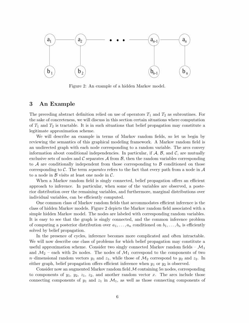
Figure 3: An example of the Markov random field M when n = 4. Note the presence ofcycles.
y2 and z2 in M2. Furthermore, 2n additional arcs connect each component of x withcomponents of z1 and z2. As illustrated by an example in Figure 3, M can possess cycles.In the presence of cycles, traditional exact inference method [16] requires construction of ajunction tree, where nodes in the tree correspond to cliques in a triangulated graph. Theresulting clique is generally very large due to the presence of cycles. Since the running timeof these algorithms is exponential in the clique size, exact inference is typically infeasible inthese problems.
Though the presence of cycles can render many inference tasks intractable, there areat least some forms of inference in M that can be performed efficiently. For example,upon observation of y1, the posterior distribution p∗1 over x can be efficiently computedby belief propagation. This is possible because the nodes corresponding to z2 and y2 canbe ignored, and the remaining nodes form a singly connected graph. Similarly, if y2 isobserved, the posterior distribution p∗2 over x can be efficiently inferred. However, if weobserve both y1 and y2, inference becomes complex. In this context, belief propagation mayprovide a suitable approximation algorithm. Ideally, the algorithm should generate marginaldistributions over individual components of x, conditioned on simultaneous observation ofy1 and y2.
We assume that the prior distribution p0 over x factors (i.e., p0 = πp0, or equivalently,the components of x are initially independent). For any density g over x, p∗1g/p0 would bethe posterior density over x conditioned on y1 if the prior density over x were g, rather thanp0. Consequently, for any density g that factors, by appropriately altering the priors on x(while keeping fixed conditional probabilities of y1 and z1, conditioned on x) and applyingbelief propagation, we can efficiently compute π(p∗1g/p0). This in turn enables efficientcomputation of
T1g = α
(
π
(
p∗1g
p0
)
p0
g
)
,
since pointwise multiplication and normalization are tractable for functions that factor. The
7

operator T2 similarly accommodates efficient computation.In conclusion, for the Markov random field M, there are tractable implementations of
T1 and T2, and application of belief propagation is therefore feasible. Whether or not beliefpropagation will generate useful approximations, however, is a separate issue.
4 The Gaussian Case
In the remainder of this paper, we will focus on a setting in which the joint distribution ofx, y1, and y2, is Gaussian. In this context, application of belief propagation may appearto be unwarranted – there are tractable algorithms for computing conditional distributionswhen priors are Gaussian. Indeed, our primary motivation is to provide a setting amenableto a streamlined analysis and concise results. It is worth noting, nevertheless, that beliefpropagation may provide a more efficient means than traditional algorithms for solving cer-tain Gaussian inference problems. We will further discuss this possibility in the concludingsection.
Let us define some notation that will facilitate our exposition. Let D denote the set ofcovariance matrices that are diagonal and positive definite. Let G denote the set of Gaussiandensities with covariance matrices in D. We will write g ∼ N(µg,Σg) to denote a Gaussiandensity g with mean vector µg and covariance matrix Σg. For any matrix A, let δ(A) denotea diagonal matrix with entries equal to the diagonal elements of A. Hence,
πg ∼ N(µg, δ(Σg)),
for any Gaussian density g ∼ N(µg,Σg). For any diagonal matrices D and D, we writeD ≤ D if Dii ≤ Dii for all i and D < D if Dii < Dii for all i. For any two pairs ofdiagonal matrices (C,D) and (C,D), we write (C,D) ≤ (C,D) if C ≤ C and D ≤ D.Similarly, we write (C,D) < (C,D) if C < C and D < D. For any matrices Σu,Σv forwhich Σ−1
u + Σ−1v − I is nonsingular, we define a matrix AΣu,Σv by
AΣu,Σv = (Σ−1u + Σ−1
v − I)−1.
To abbreviate, we will sometimes denote this matrix by Auv. Finally, all vectors are assumedto be column vectors unless explicitly stated otherwise.
When the random variables x, y1, and y2, are jointly Gaussian, the densities p∗1, p∗2, f ,and p0, are also Gaussian. We define µ, µ1, µ2, Σ, Σ1, and Σ2, to be means and covariancematrices satisfying
p∗1 ∼ N(µ1,Σ1), p∗2 ∼ N(µ2,Σ2), f ∼ N(µ,Σ).
We make the following assumptions concerning these parameters.
Assumption 1(a) p0 = N(0, I), where I is the identity matrix.(b) Σ−1
1 − I and Σ−12 − I are positive definite.
(c) Σ1 and Σ2 are positive definite.
The first assumption simplifies the exposition at no sacrifice of generality. Any problemwith a nondegenerate Gaussian prior on x can be transformed to meet this requirement
8

by appropriate translation and scaling of the coordinate system. The second assumptionimplies that the observations y1 and y2 each provide at least some information pertinentto every component of x. The final assumption, on the other hand, requires that neitherobservation rules out possible outcomes – every outcome for x is possible both before andafter an observation, though the prior and posterior probabilities may differ substantially.
Since f = α(p∗1p∗2/p0), its mean µ and covariance matrix Σ are determined by those of
p∗1, p∗2, and p0. The nature of this dependence is identified by the following lemma, whichwill be reused for various purposes in subsequent sections.
Lemma 1 Let u ∼ N(µu,Σu) and v ∼ N(µv,Σv), where Σu and Σv are positive definite.If Σ−1
u + Σ−1v − I is positive definite, then
α
(
uv
p0
)
∼ N(
Auv
(
Σ−1u µu + Σ−1
v µv
)
, Auv
)
.
This result follows from simple algebra, and we omit the proof. The implications withrespect to µ and Σ are, of course, that
µ = AΣ1,Σ2
(
Σ−11 µ1 + Σ−1
2 µ2
)
and Σ = AΣ1,Σ2 .
It turns out that, if initialized with Gaussian densities q(0)1 , q
(0)2 ∈ G, all iterates q
(k)1
and q(k)2 generated by belief propagation are also in G. This fact simplifies analysis of the
algorithm’s dynamics – we need only attend to sequences of means and covariance matrices.
In particular, we can define sequences m(k)1 , m
(k)2 , C
(k)1 , and C
(k)2 , such that
q(k)1 ∼ N
(
m(k)1 , C
(k)1
)
and q(k)2 ∼ N
(
m(k)2 , C
(k)2
)
.
The fact that iterates remain Gaussian is a consequence of the following lemma, the proofof which is provided in Appendix B.
Lemma 2 The set G is closed under T1 and T2.
It follows from this lemma that, over the domain G, the mappings T1 and T2, which acton densities, can be represented in terms of operations on mean vectors and covariancematrices. We will provide characterizations of these operations in the form of a lemma. Fora concise statement of the lemma, let us define some notation. For any D ∈ D, let functionsF1 and F2 be defined by
F1(D) =(
(δ (AΣ1,D))−1 + I −D−1)−1
,
and
F2(D) =(
(δ (AD,Σ2))−1 + I −D−1
)−1.
Furthermore, for any m ∈ <n and any D ∈ D, let functions H1 and H2 be defined by
H1(m,D) = F1(D)(
A−1F1(D),DAΣ1,D − I
)
D−1m + F1(D)A−1F1(D),DAΣ1,DΣ−1
1 µ1,
and
H2(m,D) = F2(D)(
A−1D,F2(D)AD,Σ2 − I
)
D−1m + F2(D)A−1D,F2(D)AD,Σ2Σ
−12 µ2.
The lemma follows.
9
Lemma 3 For all g ∈ G, if g ∼ N(µg, Dg) then
T1g ∼ N(H1(µg, Dg),F1(Dg)) and T2g ∼ N(H2(µg, Dg),F2(Dg)).
Given this lemma, dynamics of belief propagation can be characterized by
C(k+1)1 = F1
(
C(k)2
)
and C(k+1)2 = F2
(
C(k)1
)
,
andm
(k+1)1 = H1
(
m(k)2 , C
(k)2
)
and m(k+1)2 = H2
(
m(k)1 , C
(k)1
)
.
Once again, we postpone the proof of this lemma to Appendix B.
5 Convergence Analysis
Two immediate consequences of Lemma 3 guide the general structure of our convergenceanalysis. The first is that covariance matrices generated by belief propagation evolve in-dependently from mean vectors. This fact leads us to begin by studying the dynamics ofcovariance matrices without paying any attention to that of the mean vectors.
We will show that each sequence of covariance matrices converges to a unique stationarypoint. Denoting the stationary points by C∗
1 and C∗2 , this allows us to approximate the
dynamics of the means for large k by
m(k+1)1 = H1
(
m(k)2 , C∗
2
)
and m(k+1)2 = H2
(
m(k)1 , C∗
1
)
.
A second consequence of Lemma 3 – that the functions H1 and H2 are affine in their
first arguments – then renders the convergence analysis for m(k)1 and m
(k)2 amenable to the
tools of linear systems. Unfortunately, unlike the sequences of covariance matrices, thesequences of means do not always converge. We will, however, provide conditions underwhich convergence is guaranteed.
Stability of a particular matrix constitutes a sufficient condition for global convergenceof the mean vectors. We will show that the set of Σ1 and Σ2 that lead to stability ofthis matrix is invariant under a certain type of transformation. In addition, to facilitateunderstanding, we will provide simpler conditions under which the matrix is stable. Asa preview, let us state – in rough terms – three such conditions, each of which ensuresconvergence:
1. Σ1 and Σ2 are “complementary.” (Proposition 2)
2. Either Σ1 or Σ2 is diagonal or “nearly diagonal.” (Proposition 3 and 4)
3. Σ1 and Σ2 are “well-conditioned.” In other words, for each matrix, the ratio of thelargest to the smallest eigenvalue is not large. (Proposition 5)
In analyzing each of the above conditions, we will use a customized argument. A unifiedapproach that offers interpretable means to distinguishing convergent cases from those thatare not would be desirable, but finding such an approach remains an open problem.
Let us now move on to formal statements of our results and the corresponding analyses.The following subsection addresses convergence of the sequences of covariance matrices,while dynamics of the mean vectors are treated in Section 5.2.
10

5.1 Convergence of the Covariance Matrices
Defining F byF(D1, D2) = (F1(D2),F2(D1)) ,
for all D1, D2 ∈ D, it is clear from Lemma 3 that(
C(k)1 , C
(k)2
)
= Fk(
C(0)1 , C
(0)2
)
.
The following theorem establishes that such a sequence converges to a point that is inde-pendent of the initial iterate.
Theorem 1 The operator F possesses a unique fixed point in D×D. Furthermore, denotingthis fixed point by (C∗
1 , C∗2 ),
limk→∞
Fk(D1, D2) = (C∗1 , C∗
2 ) ,
for all D1, D2 ∈ D.
Since the operator F is uniquely determined by Σ1 and Σ2, it follows from Theorem 1that the unique fixed point (C∗
1 , C∗2 ) is completely determined by Σ1 and Σ2, which are
the covariance matrices of the conditional densities p∗1 and p∗2, respectively. For ease ofexposition, we do not make explicit the dependence of C ∗
1 and C∗2 on Σ1 and Σ2. The
proof of Theorem 1 relies on the following lemma. The first lemma captures the essentialproperties of the operator F . The proof of this result is given in Appendix C
Lemma 4(a) Continuity: The function F is continuous on D ×D.(b) Monotonicity: For all X1, X2, Y1, Y2 ∈ D, if (X1, X2) ≤ (Y1, Y2), then
F(X1, X2) ≤ F(Y1, Y2).
(c) Boundedness: There exist matrices D1, D2 ∈ D such that for all D1, D2 ∈ D,(
D1, D2
)
≤ F(D1, D2) < (I, I) .
(d) Scaling: For all β ∈ (0, 1) and D1, D2 ∈ D,
βF (D1, D2) < F (βD1, βD2) .
The following lemma establishes convergence when the sequence of covariance matricesis initialized with the identity matrix.
Lemma 5 The sequence Fk(I, I) converges in D ×D to a fixed point of F .
Proof: By Lemma 4(c), F(I, I) < (I, I). It then follows from monotonicity (Lemma 4(b))that Fk+1(I, I) ≤ Fk(I, I). Because Fk(I, I) is bounded below by a pair of matrices in D(Lemma 4(c)), the sequence must converge in D×D. Furthermore, because F is continuouson D ×D (Lemma 4(a)), the limit limk→∞Fk(I, I) must be a fixed point of F .
Let (C∗1 , C∗
2 ) = limk→∞Fk(I, I). (By Lemma 5, the limit exists and C∗1 , C∗
2 ∈ D.) Thefollowing lemma establishes this as the unique fixed point in D ×D.
11

Lemma 6 (C∗1 , C∗
2 ) is the unique fixed point in D ×D of F .
Proof: By Lemma 5, (C∗1 , C∗
2 ) is a fixed point of F . Let (D1, D2) ∈ D × D be a differentfixed point. It follows from Lemma 4(c) that (D1, D2) ≤ (I, I). By monotonicity (Lemma4(b)),
(D1, D2) = Fk (D1, D2) ≤ Fk (I, I) ,
for all k. Hence, (D1, D2) ≤ (C∗1 , C∗
2 ) .Let
β = sup{
γ ∈ (0, 1]∣
∣
∣ (γC∗1 , γC∗
2 ) ≤ (D1, D2)}
.
Note that β is well–defined because D1 and D2 are positive definite. Furthermore, since(D1, D2) 6= (C∗
1 , C∗2 ), we have β < 1. It follows from Lemma 4(d) that
β (C∗1 , C∗
2 ) = βF (C∗1 , C∗
2 ) < F (βC∗1 , βC∗
2 ) .
In addition, due to monotonicity of F (Lemma 4(b)),
F (βC∗1 , βC∗
2 ) ≤ F (D1, D2) = (D1, D2) .
Hence,(βC∗
1 , βC∗2 ) < (D1, D2) ,
which implies existence of some α > 0 such that
(α + β) (C∗1 , C∗
2 ) ≤ (D1, D2) .
However, this contradicts the definition of β. It follows that (C ∗1 , C∗
2 ) is the unique fixedpoint of F in D ×D.
5.1.1 Proof of Theorem 1
Lemma 6 established uniqueness of a fixed point (C ∗1 , C∗
2 ) and Lemma 5 asserts that Fk(I, I)converges to this fixed point. To complete the proof of Theorem 1, we need to show thatFk(D1, D2) converges for all D1, D2 ∈ D, not only D1 = D2 = I.
If (C∗1 , C∗
2 ) ≤ (D1, D2) ≤ (I, I) convergence to (C∗1 , C∗
2 ) follows from monotonicity(Lemma 4(b)). In particular, (C∗
1 , C∗2 ) = Fk(C∗
1 , C∗2 ) ≤ Fk(D1, D2) ≤ Fk(I, I), and since
Fk(I, I) converges to (C∗1 , C∗
2 ), so must Fk(D1, D2).For the more general case of (D1, D2) ≥ (C∗
1 , C∗2 ), convergence follows from the fact
that (C∗1 , C∗
2 ) = F(C∗1 , C∗
2 ) ≤ F(D1, D2) < (I, I) (a consequence of Lemmas 4(b) and 4(c)).Considering F(D1, D2) as a starting point for the sequence leads to the preceding case forwhich we have already established convergence.
Let us now address the case of (D1, D2) ≤ (C∗1 , C∗
2 ). Let
β = sup{
γ ∈ (0, 1]∣
∣
∣ (γC∗1 , γC∗
2 ) ≤ (D1, D2)}
.
By Lemma 4(d),(βC∗
1 , βC∗2 ) ≤ F (βC∗
1 , βC∗2 ) .
It follows from monotonicity (Lemma 4(b)) that,
Fk (βC∗1 , βC∗
2 ) ≤ Fk+1 (βC∗1 , βC∗
2 ) ≤ Fk+1 (D1, D2) ≤ (C∗1 , C∗
2 )
12

for all k. Hence, Fk (βC∗1 , βC∗
2 ) converges in D × D, and since F is continuous, the limitmust be a fixed point. Uniqueness of the fixed point (C ∗
1 , C∗2 ) makes it the only viable limit.
Since(βC∗
1 , βC∗2 ) ≤ (D1, D2) ≤ (C∗
1 , C∗2 ) ,
Fk (D1, D2) must also converge to (C∗1 , C∗
2 ) by monotonicity.To complete the proof, we consider the case of an arbitrary pair D1, D2 ∈ D. For this
case, there exist matrices D,D ∈ D such that D ≤ C ∗i ≤ D and D ≤ Di ≤ D for i = 1, 2.
By monotonicity,
Fk (D,D) ≤ Fk (D1, D2) ≤ Fk(
D,D)
.
Our previous arguments establish that F k(D,D) and Fk(D,D) both converge to (C∗1 , C∗
2 ),and consequently Fk(D1, D2) must also converge to (C∗
1 , C∗2 ).
5.2 Convergence of the Mean Vectors
Unlike the sequences of covariance matrices, the sequences of mean vectors do not alwaysconverge. In this section, we establish sufficient conditions that ensure convergence. Wewill first show that convergence is guaranteed by the stability of a certain matrix TΣ1,Σ2 ,defined by
TΣ1,Σ2 =
(
0 A−1C∗
1 ,C∗
2AΣ1,C∗
2− I
A−1C∗
1 ,C∗
2AC∗
1 ,Σ2 − I 0
)
.
Unfortunately, this matrix and the factors influencing its stability are difficult to interpret.Consequently, the remainder of this section will be devoted to understanding properties ofthose Σ1 and Σ2 that give rise to a stable TΣ1,Σ2 and to establishing interpretable conditionsthat ensure stability, and thus, convergence of the mean vectors.
Let us begin by stating and proving the result linking convergence to stability of TΣ1,Σ2 .For the purpose of this theorem as well as the associated analysis, we will denote the spectralradius of any matrix A by ρ(A).
Theorem 2 If ρ (TΣ1,Σ2) < 1, then there exist vectors m∗1 and m∗
2 such that, for any
m(0)1 ,m
(0)2 and any C
(0)1 , C
(0)2 ∈ D, the sequence (m
(k)1 ,m
(k)2 ) converges to (m∗
1,m∗2).
This theorem provides a sufficient and “almost necessary” condition for convergence.However, because the matrix TΣ1,Σ2 is difficult to interpret, this condition offers littleinsight into factors influencing convergence. After proving Theorem 2, we will provide insubsequent subsections more interpretable conditions under which ρ(TΣ1,Σ2) < 1. Let usnow move on to prove Theorem 2. We will rely on a lemma that is somewhat standard inflavor. We state the result here and provide its proof in Appendix D.
Lemma 7 Let {Ak} be a sequence of matrices that converges to A, and let {bk} be asequence of vectors that converges to b. Consider a sequence of vectors {xk} with
xk+1 = Akxk + bk,
for all k ≥ 0. If ρ(A) < 1, then there exists a vector x∗ such that the sequence {xk}converges to x∗ for any x0.
13

Proof of Theorem 2Recall from Lemma 3 that the mean vectors evolve according to
m(k+1)1 = H1
(
m(k)2 , C
(k)2
)
and m(k+1)2 = H2
(
m(k)1 , C
(k)1
)
,
which we can rewrite as
m(k+1)1 = C
(k+1)1
(
A−1
C(k+1)1 ,C
(k)2
AΣ1,C
(k)2
− I
)
(
C(k)2
)−1m
(k)2 +C
(k+1)1 A−1
C(k+1)1 ,C
(k)2
AΣ1,C
(k)2
Σ−11 µ1,
and
m(k+1)2 = C
(k+1)2
(
A−1
C(k)1 ,C
(k+1)2
AC
(k)1 ,Σ2
− I
)
(
C(k)1
)−1m
(k)1 +C
(k+1)2 A−1
C(k)1 ,C
(k+1)2
AC
(k)1 ,Σ2
Σ−12 µ2.
To highlight the relation between these dynamics and those addressed by Lemma 7, let usintroduce some additional notation. For each k, let Ck, Rk, and Tk be defined by
Ck =
(
C(k)1 0
0 C(k)2
)
, Rk =
A−1
C(k+1)1 ,C
(k)2
AΣ1,C
(k)2
0
0 A−1
C(k)1 ,C
(k+1)2
AC
(k)1 ,Σ2
,
and
Tk =
0 A−1
C(k+1)1 ,C
(k)2
AΣ1,C
(k)2
− I
A−1
C(k)1 ,C
(k+1)2
AC
(k)1 ,Σ2
− I 0
.
We then have(
m(k+1)1
m(k+1)2
)
= Ck+1 Tk Ck−1
(
m(k)1
m(k)2
)
+ Ck+1 Rk
(
Σ−11 µ1
Σ−12 µ2
)
.
Theorem 1, asserts that (C(k)1 , C
(k)2 ) converges to (C∗
1 , C∗2 ). It follows that the matrices
Ck+1, Tk, Ck−1, and Rk, converge. Furthermore, the limit of convergence of Ck+1 Tk Ck
−1
is given by(
C∗1 0
0 C∗2
)
TΣ1,Σ2
(
C∗1 0
0 C∗2
)−1
.
Since ρ(A) = ρ(MAM−1) for any matrix A and nonsingular matrix M , we have
ρ
(
C∗1 0
0 C∗2
)
TΣ1,Σ2
(
C∗1 0
0 C∗2
)−1
= ρ(TΣ1,Σ2).
The result therefore follows from Lemma 7.
5.2.1 Region of Convergence
We know from Theorem 2 that a sufficient (and almost necessary) condition for convergenceof the mean vectors is ρ (TΣ1,Σ2) < 1. Let C denote the set of (Σ1,Σ2) satisfying Assumption1 such that ρ (TΣ1,Σ2) < 1. Thus, C can be interpreted as the region in the space ofsymmetric positive definite matrices where belief propagation converges. In this section, we
14

will show that C is invariant under a certain type of transformation. This result will provideus with some information on the shape of C. In the next section, we will demonstrate thatcertain classes of “well-behaved” symmetric positive definite matrices belong to C.
Before we proceed to the main result of this section, let us introduce some notation.For any symmetric matrix A, let λmin(A) and λmax(A) denote the smallest and largesteigenvalues of A, respectively.
Proposition 1 Let
Σβ1 =
(
βΣ−11 + (1− β)
I
2
)−1
, and Σβ2 =
(
βΣ−12 + (1− β)
I
2
)−1
, β ≥ 1.
If (Σ1,Σ2) ∈ C, then(
Σβ1 ,Σβ
2
)
∈ C for all β ≥ 1.
Proof: It is not hard to verify that Σβ1 and Σβ
2 satisfy Assumption 1. Let (C∗1 , C∗
2 ) denote theunique fixed point of the sequence of covariance matrices generated by belief propagationwhen the covariance matrices of p∗1 and p∗2 are Σ1 and Σ2, respectively. Also, let
Cβ1 =
(
β (C∗1 )−1 + (1− β)
I
2
)−1
, and Cβ2 =
(
β (C∗2 )−1 + (1− β)
I
2
)−1
.
It follows from the definition of(
Σβ1 ,Σβ
2
)
and(
Cβ1 , Cβ
2
)
that
AΣβ
1 ,Cβ2
=1
βAΣ1,C∗
2, A
Cβ1 ,Σβ
2=
1
βAC∗
1 ,Σ2 , and ACβ
1 ,Cβ2
=1
βAC∗
1 ,C∗
2.
Since (C∗1 , C∗
2 ) is the unique fixed point of F (Theorem 1), it follows that
C∗1 =
(
(
δ(
AΣ1,C∗
2
))−1+ I − (C∗
2 )−1)−1
,
or equivalently
AC∗
1 ,C∗
2=(
(C∗1 )−1 + (C∗
2 )−1 − I)−1
= δ(
AΣ1,C∗
2
)
.
Thus,
ACβ
1 ,Cβ2
=1
βAC∗
1 ,C∗
2=
1
βδ(
AΣ1,C∗
2
)
=1
βδ(
βAΣβ
1 ,Cβ2
)
= δ(
AΣβ
1 ,Cβ2
)
.
Hence,
Cβ1 =
(
(
δ(
AΣβ
1 ,Cβ2
))−1+ I −
(
Cβ2
)−1)−1
.
A similar argument shows that
Cβ2 =
(
(
δ(
ACβ
1 ,Σβ2
))−1+ I −
(
Cβ1
)−1)−1
.
It follows from Theorem 1 that(
Cβ1 , Cβ
2
)
is the unique fixed point of the sequence of
covariance matrices generated by belief propagation when the covariance matrices of p∗1 and
15
p∗2 are Σβ1 and Σβ
2 , respectively. Therefore,
TΣβ
1 ,Σβ2
=
0 A−1
Cβ1 ,Cβ
2
AΣβ
1 ,Cβ2− I
A−1
Cβ1 ,Cβ
2
ACβ
1 ,Σβ2− I 0
=
(
0 A−1C∗
1 ,C∗
2AΣ1,C∗
2− I
A−1C∗
1 ,C∗
2AC∗
1 ,Σ2 − I 0
)
= TΣ1,Σ2
The desired result follows.The previous proposition provides us with some information on the shape of C. If we let
C−1 ={(
Σ−11 ,Σ−1
2
)
: (Σ1,Σ2) ∈ C}
be a collection of the inverses of covariance matrices in
C, the previous proposition suggests that there is an open set centered at(
I2 , I
2
)
such that
C−1 consists of rays emanating from the boundary of this set. Consequently, we conjecturethat the region of convergence C should be star-shaped with a center at the origin (0, 0).Currently, we do not have a formal proof of this result, but we plan to pursue this in ourfuture work. Also, this result appears to resemble a result reported in [23] (Theorem 6.2)on stability of fixed points of general turbo decoding.
5.2.2 Sufficient Conditions for ρ(TΣ1,Σ2) < 1
In the previous section, we showed that covariance matrices Σ1 and Σ2 that lead to conver-gence of the mean vectors are invariant under a certain type of transformation. This resultprovides us with information on the shape of the region of convergence. Unfortunately, itdoes not help us in determining if a particular pair of covariance matrices (Σ1,Σ2) will leadto a convergent sequence of mean vectors. In this section, we offer four sufficient conditionsthat ensure stability of the matrix TΣ1,Σ2 , and thus, convergence of the mean vectors. Sincethe proofs of these conditions are quite complicated, we defer them to the appendices. Wewill instead focus on the insights derived from each of these conditions. The first conditionis expressed in the following proposition, whose proof is given in Appendix E.
Proposition 2 For any symmetric positive definite matrix Σ such that Σ−1− I is positivedefinite, if
Σ1 =(
Σ−1 + γI)−1
, and Σ2 =(
Σ−1 − γI)−1
,
then (Σ1,Σ2) ∈ C for all − 1−λmax(Σ)λmax(Σ) < γ < 1−λmax(Σ)
λmax(Σ) .
We should note that since Σ−1− I is positive definite, all eigenvalues of Σ are less thanone. This implies that the range of allowable γ’s in Proposition 2 includes zero. So, ifS = {(Σ1,Σ2) : Σ1 = Σ2}, it follows that there is an open set U containing S such thatρ (TΣ1,Σ2) < 1 for all (Σ1,Σ2) ∈ U . Thus, whenever Σ1 and Σ2 are equal or “close”, themean vectors converge.
In general, Proposition 2 shows that the mean vectors will converge if the covariancematrices Σ1 and Σ2 are “complementary” in the sense that the total variance, as measured
by(
Σ−11 + Σ−1
2
)−1, is not too large. The degree of “complementarity” between Σ1 and Σ2
is captured by the parameter γ. As γ increases, the variance of Σ1 decreases (relative to
16
Σ) while that of Σ2 increases. This might correspond to the situation in which additionalerrors are introduced, resulting in greater uncertainty over the expected value of x giveny2 (thus, the increase in the variance of Σ2). Proposition 2 tells us that belief propagationstill converges, provided that there is a corresponding increase in the precision associatedwith the estimate of the expected value of x given y1 (i.e., a decrease in the variance ofΣ1). Furthermore, if we start with a fairly certain estimate of x (λmax(Σ) ≈ 0), we see thatbelief propagation would still converge despite a wide range of variation in the covariancematrices, since the range of γ is inverse proportional to the largest eigenvalue of Σ.
Whether or not we are dealing with Gaussians, when the components of x conditionedon y1 are independent – or equivalently, p∗1 factors – it is easy to see that belief propagationconverges to πf . Since p∗1 factors, it follows that for any density q,
T1q = α
((
πp∗1q
p0
)
p0
q
)
= p∗1,
which implies that q(k)1 = p∗1 for k ≥ 1. Furthermore, note that
T2p∗1 = α
((
πp∗1p
∗2
p0
)
p0
p∗1
)
= α
(
(πf)p0
p∗1
)
.
Therefore, we have
α
(
q(k)1 q
(k)2
p0
)
= πf,
for k ≥ 2. Independence of components of x conditioned on y2 leads to an analogousoutcome.
In the Gaussian case, independence corresponds to the fact that a covariance matrix isdiagonal. The argument we have discussed in the context of general distributions impliesthat belief propagation converges when either Σ1 or Σ2 is diagonal. However, a strongerresult, formalized in the following proposition, establishes that convergence holds for a rangeof matrices that are “nearly diagonal.” The proof of this proposition is given in AppendixF.
Proposition 3 For i = 1, 2, let Li and Ui be defined by
Li = 1− λmin
(
Σi (δ (Σi))−1)
and Ui = λmax
(
Σiδ(
Σ−1i
))
− 1.
If2∏
i=1
(Li ∨ Ui) < 1,
then ρ (TΣ1,Σ2) < 1.
Let us discuss a certain interpretation of the proposition. When Σ1 is diagonal, L1 =U1 = 0 and
∏2i=1 (Li ∨ Ui) = 0. This is an extreme case that leaves much leeway in the
requirement that∏2
i=1 (Li ∨ Ui) < 1. An analogous extreme case arises when Σ2 is diagonal.As Σ1 becomes “less diagonal,” L1 and U1 grow – the former is bounded by 1 but the
latter can become arbitrarily large. In any event, L1∨U1 can be viewed as a measure of howfar Σ1 is from being diagonal, or alternatively, how correlated the components of x become
17
upon observation of y1. Furthermore, the product∏2
i=1 (Li ∨ Ui) combines this measure forΣ1 and Σ2, and the requirement for this product to be less than 1 allows for one covariancematrix to become more diagonal as the other becomes less so.
Proposition 3 places constraints on Σ1 and Σ2 under which convergence is guaranteed,and we discussed how covariance matrices that are “nearly diagonal” should satisfy suchconstraints. The next proposition extends this result further by showing that if the off-diagonal elements of Σ1 and Σ2 are small relative to the diagonal elements, then beliefpropagation converges. The proof of this proposition follows directly from Proposition 3,and we refer the reader to Appendix G.
Proposition 4 For any Σ1 and Σ2 satisfying Assumption 1, let
Σβ1 =
(
Σ−11 + (β − 1)I
)−1, and Σβ
2 =(
Σ−12 + (β − 1)I
)−1.
Then, there exist UΣ1,Σ2 > 1 such that ρ(
TΣβ
1 ,Σβ2
)
< 1 for all β > UΣ1,Σ2.
Let us discuss an interpretation of the above result in coding context. The covariancematrices Σβ
1 and Σβ2 can be written as
Σβ1 =
(
Σ−11 +
(
1
βI
)−1
− I
)−1
, and Σβ2 =
(
Σ−12 +
(
1
βI
)−1
− I
)−1
.
It follows from Lemma 1 that Σβ1 can be interpreted as the covariance matrix of the con-
ditional density of x given y1, when the prior density p0 of x has variance 1β I instead of I.
A similar interpretation applies to Σβ2 . As β increases, the uncertainty over the prior esti-
mate of the random variable x decreases. Thus, β can be thought of as the signal-to-noiseratio of x. Moreover, recall that Σ1 and Σ2 represent the covariances of the conditionaldensity of x given y1 and y2, respectively. These covariances encapsulate the correlationsamong information bits conditioned on the observed transmissions. These correlations aredetermined by the encoding scheme and the channel characteristics. Viewing from this per-spective, the result of Proposition 4 implies that, for a given encoding scheme and channelcharacteristics, there is a threshold UΣ1,Σ2 such that if the signal-to-noise ratio exceeds thisthreshold, then belief propagation converges. This result appears to be related to resultsreported in [1, 7, 25].
It was observed by Agrawal and Vardy [1] that for codes with finite length, there are twothresholds L and U such that when the signal-to-noise ratio is higher than U , turbo decodingconverges, but when the signal-to-noise ratio is below L, the algorithm diverges. We expectthat a similar result should hold in our context of Gaussian densities. Unfortunately, wecurrently do not have a formal proof this result. We plan to pursue this in our future work.
The last two propositions show that if the covariance matrices are “close” to diagonal,then the mean vectors converge. Here, we identify an additional situation where convergenceoccurs, which involves covariance matrices that are “well–conditioned.” This result is statedin the following proposition, whose proof is given in Appendix H.
Proposition 5 Ifλmin (Σ1)
λmax (Σ1)+
λmin (Σ2)
λmax (Σ2)> 1,
then ρ (TΣ1,Σ2) < 1.
18

As an immediate corollary of this proposition, we have ρ(TΣ1,Σ2) < 1 if
λmax (Σi)
λmin (Σi)< 2
for i = 1, 2. Hence, the means converge if the covariance matrices are “well–conditioned.”
5.2.3 Example of Divergence
In this section, we provide an example that demonstrates the possibility of a divergentsequence of mean vectors. We should note that when Σi is a 2 × 2 matrix, the variable Ui
in Proposition 3 is bounded by 1. This implies that belief propagation will converge if Σ1
and Σ2 are 2× 2 matrices. So, consider the following 3× 3 matrices
Σ1 =
0.2158720 0.3135334 0.18440280.3135334 0.5006464 0.33641290.1844028 0.3364129 0.2653747
,
and
Σ2 =
0.0346151 −0.0211820 0.0274089−0.0211820 0.0157915 −0.0175615
0.0274089 −0.0175615 0.0250863
.
For this particular choice of Σ1 and Σ2, it turns out that
C∗1 =
0.0095633 0 00 0.0157210 00 0 0.0255243
,
and
C∗2 =
0.0145617 0 00 0.0050802 00 0 0.0072025
.
With this information, it is not hard to verify that ρ(TΣ1,Σ2) = 1.0132513. Thus, the meanvectors diverge.
6 Analysis of the Fixed Point
We have established that the covariance matrices generated by belief propagation converge,and under certain conditions, so do the means. In this section, we will show that the limitsof convergence may provide useful information relating to the desired posterior densityf ∼ N(µ,Σ). In particular, it turns out – somewhat surprisingly – that the mean of theapproximation resulting from belief propagation coincides with that of f . To formalizethis result, let the limiting means and covariance matrices be denoted by m∗
1, m∗2, C∗
1 ,and C∗
2 . Furthermore, let q∗1 and q∗2 be the limiting densities with q∗1 ∼ N(m∗1, C
∗1 ) and
q∗2 ∼ N(m∗2, C
∗2 ). The following theorem establishes the main result of this section: the
mean of the density α (q∗1q∗2/p0) generated by belief propagation coincides with that of the
desired posterior density f .
19

Theorem 3 Let (C∗1 , C∗
2 ) denote the limit of the sequence of covariance matrices(
C(k)1 , C
(k)2
)
.
Suppose that sequences of the mean vectors m(k)1 and m
(k)2 converge to m∗
1 and m∗2, respec-
tively. If q∗1 ∼ N(m∗1, C
∗1 ) and q∗2 ∼ N(m∗
2, C∗2 ), then
α(q∗1q∗2/p0) ∼ N(µ,AC∗
1 ,C∗
2).
Our proof of this theorem relies on the following lemma, which provides an equationrelating means associated with the fixed points. It is not hard to show that AC∗
1 ,C∗
2, AΣ1,C∗
2,
and AC∗
1 ,Σ2 , which are used in the statement, are well–defined.
Lemma 8 Let (C∗1 , C∗
2 ) denote the limit of the sequence of covariance matrices(
C(k)1 , C
(k)2
)
.
Suppose that sequences of the mean vectors m(k)1 and m
(k)2 converge to m∗
1 and m∗2, respec-
tively. If q∗1 ∼ N(m∗1, C
∗1 ) and q∗2 ∼ N(m∗
2, C∗2 ), then
AC∗
1 ,C∗
2
(
C∗1−1m∗
1 + C∗2−1m∗
2
)
= AΣ1,C∗
2
(
Σ−11 µ1 + C∗
2−1m∗
2
)
= AC∗
1 ,Σ2
(
C∗1−1m∗
1 + Σ−12 µ2
)
.
Proof: Let q∗1 ∼ N(m∗1, C
∗1 ) and q∗2 ∼ N(m∗
2, C∗2 ). Since q∗1 and q∗2 denote the fixed points
of belief propagation, we have
q∗1 = T1q∗2 and q∗2 = T2q
∗1.
It follows that
αq∗1q
∗2
p0= απ
p∗1q∗2
p0= απ
q∗1p∗2
p0.
The result is then a consequence of Lemma 1 and the fact that π does not alter the meanof a density.
Proof of Theorem 3By Lemma 1, µ = AΣ1,Σ2
(
Σ−11 µ1 + Σ−1
2 µ2
)
, while the mean of α(q∗1q∗2/p0) is
AC∗
1 ,C∗
2
(
C∗1−1m∗
1 + C∗2−1m∗
2
)
. We will show that these two expressions are equal.
Multiplying the equations from Lemma 8 by appropriate matrices, we obtain
A−1Σ1,C∗
2AC∗
1 ,C∗
2
(
C∗1−1m∗
1 + C∗2−1m∗
2
)
= Σ−11 µ1 + C∗
2−1m∗
2,
andA−1
C∗
1 ,Σ2AC∗
1 ,C∗
2
(
C∗1−1m∗
1 + C∗2−1m∗
2
)
= C∗1−1m∗
1 + Σ−12 µ2.
It follows that(
A−1Σ1,C∗
2+ A−1
C∗
1 ,Σ2
)
AC∗
1 ,C∗
2
(
C∗1−1m∗
1 + C∗2−1m∗
2
)
= Σ−11 µ1 + Σ−1
2 µ2 + C∗1−1m∗
1 + C∗2−1m∗
2,
which implies that(
(A−1Σ1 ,C∗
2+ A−1
C∗
1 ,Σ2)AC∗
1 ,C∗
2− I
)
(
C∗1−1m∗
1 + C∗2−1m∗
2
)
= Σ−11 µ1 + Σ−1
2 µ2.
Therefore,(
A−1Σ1,C∗
2+ A−1
C∗
1 ,Σ2−A−1
C∗
1 ,C∗
2
)
AC∗
1 ,C∗
2
(
C∗1−1m∗
1 + C∗2−1m∗
2
)
= Σ−11 µ1 + Σ−1
2 µ2.
Note that A−1Σ1,C∗
2+ A−1
C∗
1 ,Σ2−A−1
C∗
1 ,C∗
2= A−1
Σ1,Σ2. It follows that
AC∗
1 ,C∗
2
(
C∗1−1m∗
1 + C∗2−1m∗
2
)
= AΣ1,Σ2(Σ−11 µ1 + Σ−1
2 µ2) = µ.
20
0 10 20 30 400
20
40
60
80
Relative Errors Between the Mean of π fand that of α(q
1(k) q
2(k)/p
0)
Iteration Number
%
0 10 20 30 405
10
15
20
25
30
35
40
Relative Errors Between the Covarianceof π f and that of α(q
1(k) q
2(k)/p
0)
Iteration Number
%
0 10 20 30 4030
40
50
60
70
80
90
100
Relative Errors Between the Mean of p1* and that of q
1(k)
Iteration Number
%
0 10 20 30 4020
40
60
80
100
Relative Errors Between the Mean of p2* and that of q
2(k)
Iteration Number
%
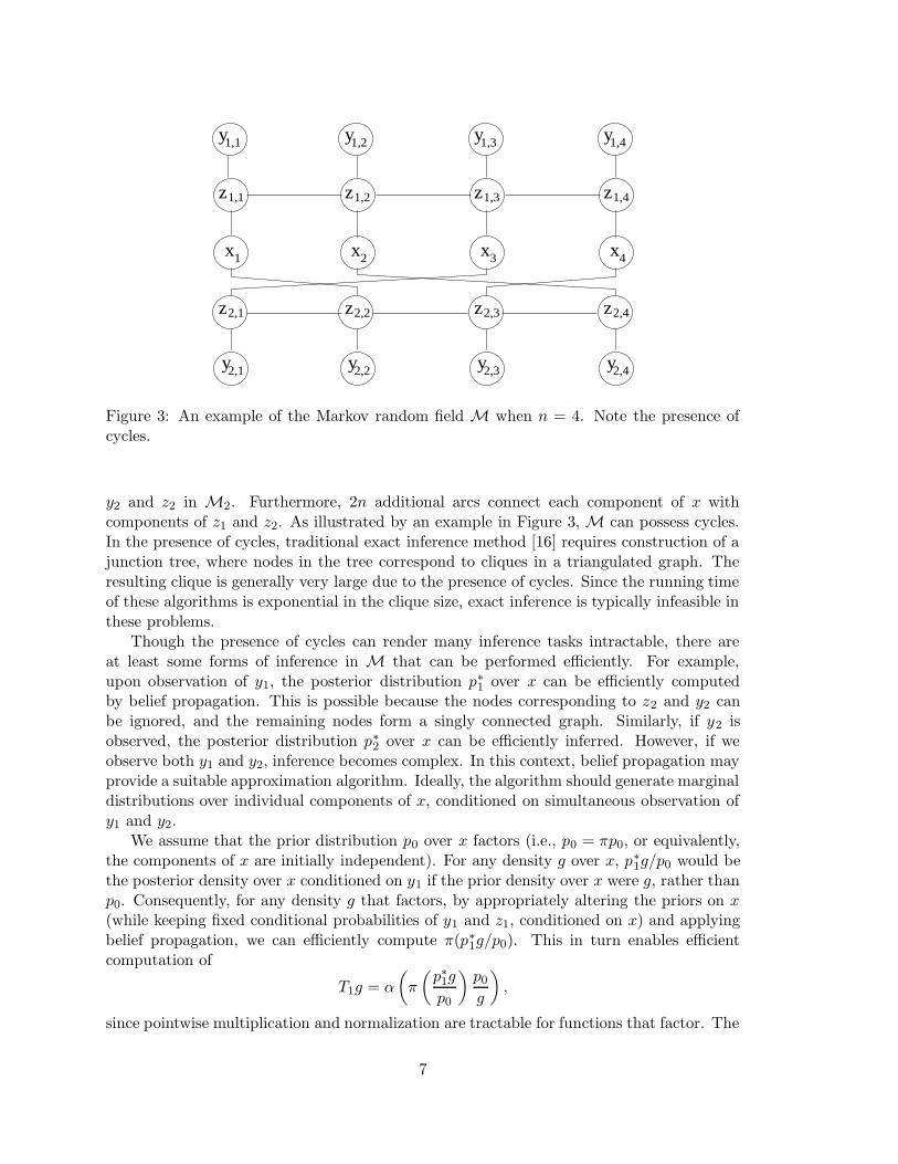
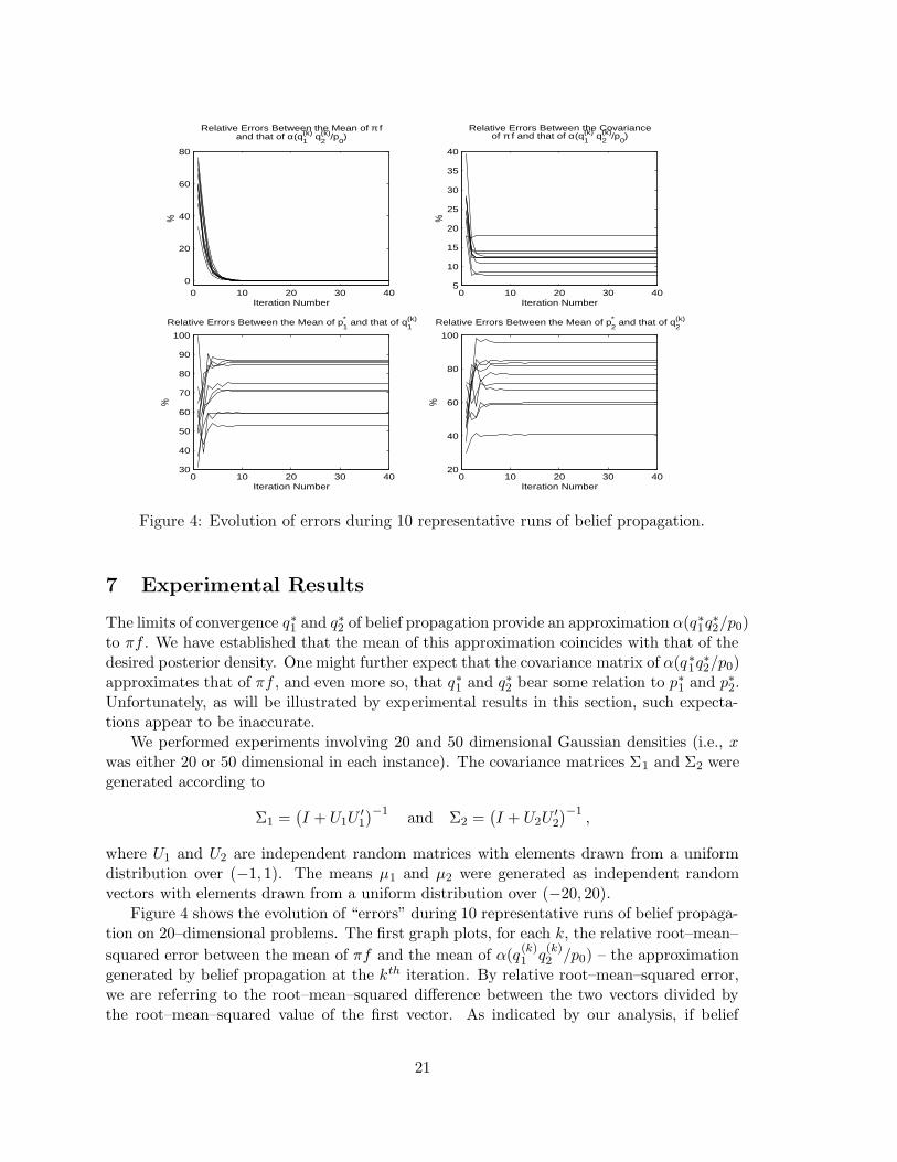
Figure 4: Evolution of errors during 10 representative runs of belief propagation.
7 Experimental Results
The limits of convergence q∗1 and q∗2 of belief propagation provide an approximation α(q∗1q∗2/p0)
to πf . We have established that the mean of this approximation coincides with that of thedesired posterior density. One might further expect that the covariance matrix of α(q∗1q
∗2/p0)
approximates that of πf , and even more so, that q∗1 and q∗2 bear some relation to p∗1 and p∗2.Unfortunately, as will be illustrated by experimental results in this section, such expecta-tions appear to be inaccurate.
We performed experiments involving 20 and 50 dimensional Gaussian densities (i.e., xwas either 20 or 50 dimensional in each instance). The covariance matrices Σ1 and Σ2 weregenerated according to
Σ1 =(
I + U1U′1
)−1and Σ2 =
(
I + U2U′2
)−1,
where U1 and U2 are independent random matrices with elements drawn from a uniformdistribution over (−1, 1). The means µ1 and µ2 were generated as independent randomvectors with elements drawn from a uniform distribution over (−20, 20).
Figure 4 shows the evolution of “errors” during 10 representative runs of belief propaga-tion on 20–dimensional problems. The first graph plots, for each k, the relative root–mean–
squared error between the mean of πf and the mean of α(q(k)1 q
(k)2 /p0) – the approximation
generated by belief propagation at the kth iteration. By relative root–mean–squared error,we are referring to the root–mean–squared difference between the two vectors divided bythe root–mean–squared value of the first vector. As indicated by our analysis, if belief
21
0 200 400 600 800 10000
0.5
1
1.5
2
2.5
3x 10
−7
Relative Errors Between the Mean of π fand that of α(q
1* q
2* /p
0)
Trial Number
%
0 200 400 600 800 10004
6
8
10
12
14
16
18
Relative Errors Between the Covarianceof π f and that of α(q
1* q
2* /p
0)
Trial Number
%
0 200 400 600 800 100050
60
70
80
90
100
110
120
130
Relative Errors Between the Mean of p1* and that of q
1*
Trial Number
%
0 200 400 600 800 100040
60
80
100
120
140
Relative Errors Between the Mean of p2* and that of q
2*
Trial Number
%
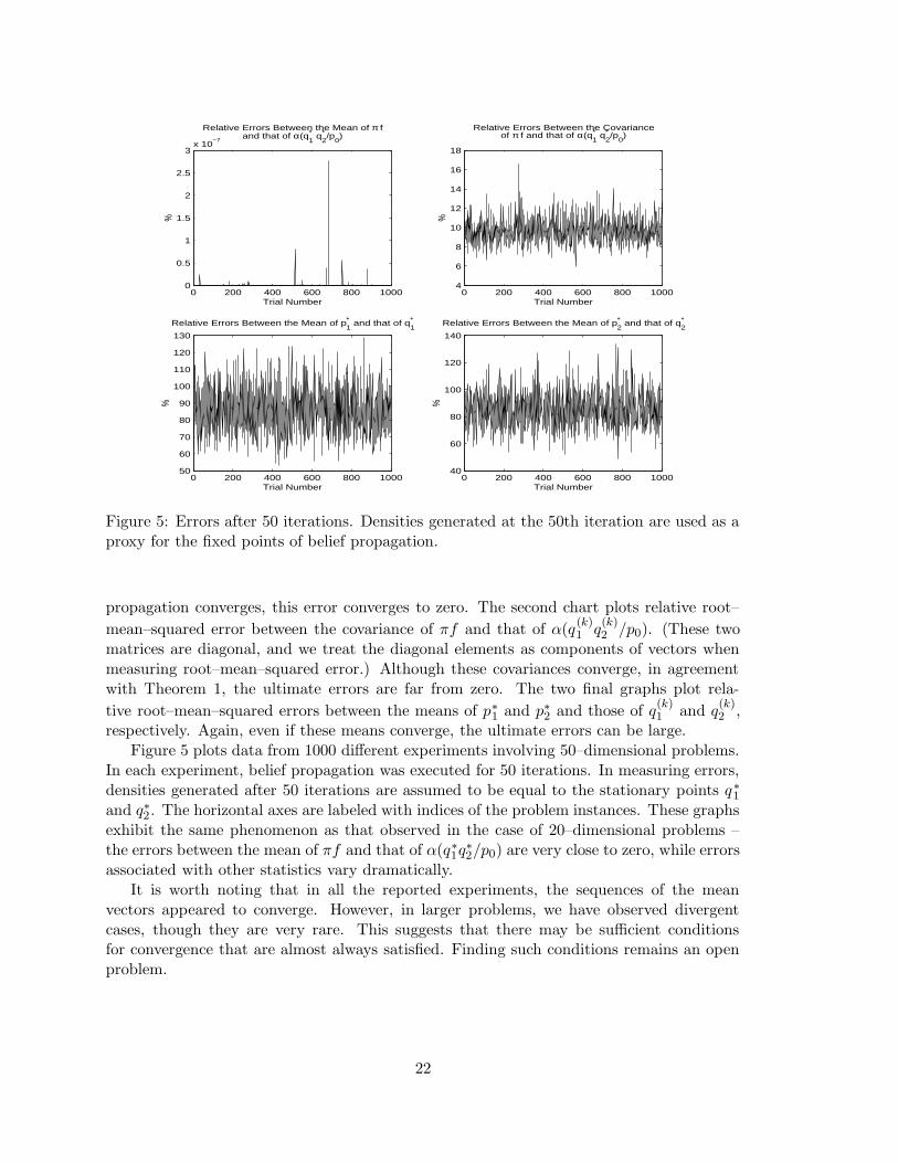
Figure 5: Errors after 50 iterations. Densities generated at the 50th iteration are used as aproxy for the fixed points of belief propagation.
propagation converges, this error converges to zero. The second chart plots relative root–
mean–squared error between the covariance of πf and that of α(q(k)1 q
(k)2 /p0). (These two
matrices are diagonal, and we treat the diagonal elements as components of vectors whenmeasuring root–mean–squared error.) Although these covariances converge, in agreementwith Theorem 1, the ultimate errors are far from zero. The two final graphs plot rela-
tive root–mean–squared errors between the means of p∗1 and p∗2 and those of q(k)1 and q
(k)2 ,
respectively. Again, even if these means converge, the ultimate errors can be large.Figure 5 plots data from 1000 different experiments involving 50–dimensional problems.
In each experiment, belief propagation was executed for 50 iterations. In measuring errors,densities generated after 50 iterations are assumed to be equal to the stationary points q∗1and q∗2. The horizontal axes are labeled with indices of the problem instances. These graphsexhibit the same phenomenon as that observed in the case of 20–dimensional problems –the errors between the mean of πf and that of α(q∗1q
∗2/p0) are very close to zero, while errors
associated with other statistics vary dramatically.It is worth noting that in all the reported experiments, the sequences of the mean
vectors appeared to converge. However, in larger problems, we have observed divergentcases, though they are very rare. This suggests that there may be sufficient conditionsfor convergence that are almost always satisfied. Finding such conditions remains an openproblem.
22
8 Closing Remarks
We have shown that, when densities are Gaussian, belief propagation often converges andthe mean associated with the limit of convergence coincides with that of the desired posteriordensity. It is intriguing to note that, in the context of communications, the objective is tochoose a code word x that comes close to the transmitted code x. One natural way to dothis involves assigning to x the code word that maximizes the conditional density f , i.e.,the one that has the highest chance of being correct. In the Gaussian case that we havestudied, this corresponds to the mean of f – a quantity that is computed correctly by beliefpropagation!
It will be interesting to explore generalizations of the line of analysis presented in thispaper. One direction might be to expand the arguments to encompass belief propagation ongeneral network topologies with Gaussian densities. A more interesting – and probably morechallenging – pursuit would be to develop theory pertaining to more general (non–Gaussian)densities.
As a parting note, let us suggest that, even in the context of Gaussian densities, be-lief propagation may prove to be useful. Let us reconsider, for example, a coupled hiddenMarkov model as that described in Section 3. Suppose now that prior distributions associ-ated with this coupled hidden Markov model are Gaussian. Then, although computation ofthe conditional mean is tractable via traditional methods, belief propagation may providea more efficient alternative, as we will now explain.
Since the densities are Gaussian, the mean of x conditioned on y1 and y2 is given by
µ =(
Σ−11 + Σ−1
2 − I)−1 (
Σ−11 µ1 + Σ−1
2 µ2
)
.
Computation of this mean may be carried out via inversion of the relevant symmetric posi-tive definite matrices, which takes on the order of n2.81 operations. Additional computationmight also be required to obtain µ1, µ2, Σ1 and Σ2.
Let us consider an alternative approach that uses belief propagation. Recall that belief
propagation computes sequences q(k)1 and q
(k)2 . As discussed in Section 3, computation of
q(k)1 and q
(k)2 at each iteration can be done efficiently via belief propagation – the procedure
requires O(n) operations per iteration. If the algorithm converges, the mean of the resultingapproximation coincides with µ. Hence, if the algorithm converges within s iterations, orat least comes very close to the limit point, we can obtain a very good approximation toµ in O (sn) operations. If s is not too large, this can result in substantial computationalsavings. Unfortunately, we do have a bound on the proximity between µ and the mean ofthe density generated by belief propagation after s iterations. Nevertheless, our experimen-tal results suggest that belief propagation converges fairly quickly. The notion that beliefpropagation might compute the mean of a posterior distribution more quickly than tradi-tional approaches raises a tantalizing possibility that the algorithm and potential variantsmight be able to accelerate the solution of many similar tasks in numerical computation.
Acknowledgments
This research was supported in part by a Stanford University Terman Award. The authorsare grateful to David Forney and Michael Jordan for pointers to literature on turbo decoding
23

and inference at early stages in this research. We also thank Michael Saunders for someuseful discussions on linear algebra. Finally, we thank anonymous reviewers for detailedthoughtful comments and suggestions.
A Lemmas on Matrix Algebra
In this section, we collect together some useful lemmas on matrix algebra. These results willbe used throughout the appendices. The first lemma states an inequality due to Bellman[4].
Lemma 9 If A is a symmetric positive definite matrix, then for all x and y
(
x′Ax)
(
y′A−1y)
≥(
x′y)2
.
It is easy to see that matrix inversion and the δ operator do not commute. The nextlemma reflects possible consequences of reordering.
Lemma 10 If A is a symmetric positive definite matrix, then
(
δ(
A−1))−1
≤ δ (A) .
Proof: By letting x = y = ei, where ei is the unit vector whose ith component is equal toone, we have
Aii
(
A−1)
ii=(
x′Ax)
(
y′A−1y)
≥(
x′y)2
= 1,
where the inequality follows from Lemma 9. It follows that
1
(A−1)ii≤ Aii,
for all i, which immediately leads to the desired result.The next lemma states an inequality due to Bergstrom [4].
Lemma 11 Let A and B be symmetric positive definite matrices. Let A(i) and B(i) denotethe sub-matrices (also symmetric positive definite) obtained by deleting the ith row andcolumn. Then,
|A|
|A(i)|+
|B|
|B(i)|≤
|A + B|
|A(i) + B(i)|,
where |M | denotes the determinant of a matrix M .
Next, we have a lemma that reflects potential consequences of distributing a certaincombination of matrix inversions and the δ operator among addends in a sum.
Lemma 12 Let A and B be symmetric positive definite matrices. Then,
(
δ(
A−1))−1
+(
δ(
B−1))−1
≤(
δ(
(A + B)−1))−1
.
24

Proof: For any nonsingular matrix A, it is well-known [27] that
(
A−1)
ii=|A (i) |
|A|
for all i. It therefore follows from Lemma 11 that
1
(A−1)ii+
1
(B−1)ii≤
1(
(A + B)−1)
ii
for all i. Equivalently,
(
δ(
A−1))−1
+(
δ(
B−1))−1
≤(
δ(
(A + B)−1))−1
.
B Proof of Lemmas 2 and 3
This appendix contains the proof of Lemmas 2 and 3. We first prove the following result,which will be used to prove Lemma 3.
Lemma 13 For all D ∈ D, F1(D) and F2(D) are positive definite diagonal matrices.
Proof: It suffices to prove this result for F1(D). The proof for F2(D) is similar. SinceΣ−1
1 − I is positive definite (Assumption 1(b)), AΣ1,D is well-defined and positive definitefor all D ∈ D. In addition, it follows from Lemma 10 that
(δ (AΣ1,D))−1 ≤ δ(
A−1Σ1,D
)
,
which implies that
(δ (AΣ1,D))−1 ≤ δ(
Σ−11
)
+ D−1 − I.
Therefore,
(δ (AΣ1,D))−1 + I −D−1 ≤ δ(
Σ−11
)
,
or equivalently,(
(δ (AΣ1,D))−1 + I −D−1)−1
≥(
δ(
Σ−11
))−1.
Using the definition of F1, it follows that
F1(D) ≥(
δ(
Σ−11
))−1,
which implies that F1(D) is a positive definite diagonal matrix.
Here is the proof of Lemma 3.
Proof: It suffices to prove this result for T1. The proof for T2 is similar. Recall thatfor any density g,
T1g = α
((
πp∗1g
p0
)
p0
g
)
25

Consider a density g ∈ G with g ∼ N (µg,Σg). Since Σ−11 −I is positive definite (Assumption
1(b)), AΣ1,Σg is positive definite. Thus, it follows from Lemma 1 that
α
(
p∗1g
p0
)
∼ N(
AΣ1,Σg
(
Σ−11 µ1 + Σ−1
g µg
)
, AΣ1,Σg
)
,
which implies that
α
(
πp∗1g
p0
)
∼ N(
AΣ1,Σg
(
Σ−11 µ1 + Σ−1
g µg
)
, δ(
AΣ1,Σg
)
)
.
It follows from the definition of F1 (Σg) and Lemma 13 that the matrix
(
δ(
AΣ1,Σg
))−1+ I − Σ−1
g
is well-defined and positive definite. Application of Lemma 1 implies that T1g is a Gaussiandensity whose covariance matrix is given by
(
(
δ(
AΣ1,Σg
))−1+ I − Σ−1
g
)−1,
which is simply F1 (Σg). Lemma 1 also tells us that the mean of the density T1g is given by
F1 (Σg)(
(
δ(
AΣ1,Σg
))−1AΣ1,Σg
(
Σ−11 µ1 + Σ−1
g µg
)
− Σ−1g µg
)
,
or equivalently,
F1 (Σg)(
(
δ(
AΣ1,Σg
))−1AΣ1,Σg − I
)
Σ−1g µg + Fg (Σg)
(
δ(
AΣ1,Σg
))−1AΣ1,ΣgΣ
−11 µ1.
Since
F1 (Σg) =(
(
δ(
AΣ1,Σg
))−1+ I − Σ−1
g
)−1,
it follows that
(
δ(
AΣ1,Σg
))−1= (F1 (Σg))
−1 + Σ−1g − I = A−1
F1(Σg),Σg.
Using this fact, the mean of the density T1g can be written as
F1 (Σg)(
A−1F1(Σg),Σg
AΣ1,Σg − I)
Σ−1g µg + Fg (Σg)A−1
F1(Σg),ΣgAΣ1,ΣgΣ
−11 µ1,
which is simply H1 (µg,Σg). Therefore,
T1g ∼ N (H1 (µg,Σg) ,F1 (Σg)) .
It is obvious that Lemma 2 is a direct corollary of Lemma 3 and 13.
26

C Proof of Lemma 4
(a) Continuity : Continuity of the operator F on its domain D × D follows immediatelyfrom its definition.
(b) Monotonicity: Let B2 = X−12 − Y −1
2 , and note that B2 ≥ 0 since X2 ≤ Y2. Startingwith the definition of AΣ1,X2 , we have
A−1Σ1,X2
= Σ−11 + X−1
2 − I = Σ−11 + Y −1
2 − I + B2 = A−1Σ1,Y2
+ B2,
which implies that
AΣ1,X2 =(
A−1Σ1,Y2
+ B2
)−1.
Since B2 ≥ 0, Lemma 12 (Appendix A) asserts that
(δ (AΣ1,X2))−1 ≥ (δ (AΣ1,Y2))
−1 +(
δ(
B−12
))−1,
and since B2 is diagonal,
(δ (AΣ1,X2))−1 ≥ (δ (AΣ1,Y2))
−1 + X−12 − Y −1
2 .
It follows that
(δ (AΣ1,X2))−1 + I −X−1
2 ≥ (δ (AΣ1,Y2))−1 + I − Y −1
2 ,
which implies that (F1 (X2))−1 ≥ (F1 (Y2))
−1, or equivalently, F1(X2) ≤ F1(Y2). An anal-ogous argument shows that F2(X1) ≤ F2(Y1). Hence, F (X1, X2) ≤ F (Y1, Y2).
(c) Boundedness: It follows from the definition of AΣ1,D2 , that
(δ (AΣ1,D2))−1 =
(
δ
(
(
Σ−11 + D−1
2 − I)−1
))−1
=(
δ(
(U + V )−1))−1
,
where U = Σ−11 − I and V = D−1
2 . From Assumption 1(b), we know that U is positivedefinite. It follows from Lemma 10 and 12 (Appendix A) that
(
δ(
U−1))−1
+(
δ(
V −1))−1
≤ (δ (AΣ1,D2))−1 ≤ δ (U + V ) .
Since V = D−12 is diagonal,
(
δ(
U−1))−1
+ D−12 ≤ (δ (AΣ1,D2))
−1 ≤ δ(
Σ−11
)
− I + D−12 ,
and since U is positive definite,
D−12 < (δ (AΣ1,D2))
−1 ≤ δ(
Σ−11
)
− I + D−12 .
It follows thatI < (δ (AΣ1,D2))
−1 + I −D−12 ≤ δ
(
Σ−11
)
.
27

Since F1(D2) =(
(δ (AΣ1,D2))−1 + I −D−1
2
)−1, we have
(
δ(
Σ−11
))−1≤ F1 (D2) < I.
An analogous argument shows that
(
δ(
Σ−12
))−1≤ F2 (D1) < I,
Hence,(
D1, D2
)
≤ F(D1, D2) < (I, I) ,
where D1 =(
δ(
Σ−11
))−1and D2 =
(
δ(
Σ−12
))−1.
(d) Scaling: We will begin by establishing that
βδ (AΣ1,D2) ≤ δ (AΣ1,βD2) .
By definition, we have
AΣ1,D2 =(
Σ−11 − I + D−1
2
)−1=(
β(
Σ−11 − I
)
+ D−12 + (1− β)
(
Σ−11 − I
))−1.
Application of Lemma 12 (Appendix A) implies that
(δ (AΣ1,D2))−1 ≥
(
δ
(
(
β(
Σ−11 − I
)
+ D−12
)−1))−1
+ (1− β)
(
δ
(
(
Σ−11 − I
)−1))−1
,
Since Σ−11 − I is positive definite (Assumption 1(b)), we have
(δ (AΣ1,D2))−1 ≥
(
δ
(
(
β(
Σ−11 − I
)
+ D−12
)−1))−1
,
which implies that
δ (AΣ1,D2) ≤ δ
(
(
β(
Σ−11 − I
)
+ D−12
)−1)
.
However,
δ
(
(
β(
Σ−11 − I
)
+ D−12
)−1)
=1
βδ
(
(
Σ−11 − I + (βD2)
−1)−1
)
=1
βδ (AΣ1,βD2) ,
which implies thatβδ (AΣ1,D2) ≤ δ (AΣ1,βD2) .
The bound on βδ(AΣ1 ,D2) implies that
(δ (AΣ1,βD2))−1 ≤
1
β(δ (AΣ1,D2))
−1 .
28

It follows that
(F1 (βD2))−1 = (δ (AΣ1,βD2))
−1 + I − (βD2)−1
≤1
β(δ (AΣ1,D2))
−1 + I −1
βD−1
2
<1
β(δ (AΣ1,D2))
−1 +1
βI −
1
βD−1
2
=1
β(F1 (D2))
−1
Therefore,βF1 (D2) < F1 (βD2) .
An analogous argument shows that
βF2 (D1) < F2 (βD1) ,
and the result follows.
D Proof of Lemma 7
The proof of Lemma 7 relies on the following two results. Because they are of standardflavor we state them without proof.
Lemma 14 Let {yk}, {αk}, and {βk} be sequences of non-negative real numbers such that
yk+1 ≤ αkyk + βk,
for all k ≥ 0. Iflim
k→∞αk = α∗ and lim
k→∞βk = 0,
where 0 < α∗ < 1, then limk→∞ yk = 0.
Lemma 15 If A is any matrix such that ρ (A) 6= 0 and ρ (A) < 1, then there exist aconstant C such that
‖An‖ ≤ Cρ (A)n
for all n.
Here is the proof of Lemma 7.
Proof: Let us first assume that ρ (A) 6= 0. Let the sequence {xk} be defined by
xk+1 = Axk + b,
for all k ≥ 0 with x0 = x0. It follows that
xk+1 − xk+1 = A (xk − xk) + (Ak −A) xk + (bk − b)
29

for all k ≥ 0. Using the above recursion, one can show that
xk+1 − xk+1 =k∑
i=0
Ai (Ak−i −A) xk−i + Ai (bk−i − b) ,
which implies that
‖xk+1 − xk+1‖ ≤k∑
i=0
‖Ai‖‖Ak−i −A‖‖xk−i‖+ ‖Ai‖‖bk−i − b‖
≤k∑
i=0
‖Ai‖‖Ak−i −A‖‖xk−i − xk−i‖+
k∑
i=0
‖Ai‖‖Ak−i −A‖‖xk−i‖+ ‖Ai‖‖bk−i − b‖
≤ C
(
k∑
i=0
ρ (A)i ‖Ak−i −A‖‖xk−i − xk−i‖
)
+
C
(
k∑
i=0
ρ (A)i ‖Ak−i −A‖‖xk−i‖+ ρ (A)i ‖bk−i − b‖
)
where the last inequality follows from Lemma 15. Define the sequence {zk} by
zk+1 = C
(
k∑
i=0
ρ (A)i ‖Ak−i −A‖‖xk−i − xk−i‖
)
+
C
(
k∑
i=0
ρ (A)i ‖Ak−i −A‖‖xk−i‖+ ρ (A)i ‖bk−i − b‖
)
.
From the definition of zk, it follows that
zk+1 = ρ (A) zk + C
(
‖Ak −A‖‖xk − xk‖+ ‖Ak −A‖‖xk−i‖+ ‖bk − b‖
)
≤
(
ρ (A) + C‖Ak −A‖
)
zk + C
(
‖Ak −A‖‖xk−i‖+ ‖bk − b‖
)
where the last inequality follows from the fact that
‖xk − xk‖ ≤ zk,
for all k ≥ 0. Since the sequence {Ak} converges to A, it follows that
limk→∞
ρ (A) + C‖Ak −A‖ = ρ (A) < 1.
Moreover, since ρ (A) < 1, the sequence {xk} converges. Thus,
limk→∞
C
(
‖Ak −A‖‖xk−i‖+ ‖bk − b‖
)
= 0.
It follows from Lemma 14 that the sequence {zk} converges to 0. Since ‖xk − xk‖ ≤ zk forall k, and the sequence {xk} converges, it follows that the sequence {xk} also converges.
30

Thus, we have established convergence of the sequence {xk} when ρ (A) 6= 0. The proof forthe case when ρ (A) = 0 is similar. The only modification is in the result of Lemma 15. Inthis case, we have
‖An‖ ≤ Cρ (A)n
for sufficiently large n. It is now easy to see that the above argument still works in thiscase.
E Proof of Proposition 2
The proof of Proposition 2 relies on the following three lemmas. The first relates stabilityof ρ(TΣ1,Σ2) to that of its two sub–matrices.
Lemma 16 If
ρ(
A−1C∗
1 ,C∗
2AΣ1,C∗
2− I
)
ρ(
A−1C∗
1 ,C∗
2AC∗
1 ,Σ2 − I)
< 1,
then ρ (TΣ1,Σ2) < 1.
Proof: Recall that the matrix TΣ1,Σ2 is defined by
TΣ1,Σ2 =
(
0 A−1C∗
1 ,C∗
2AΣ1,C∗
2− I
A−1C∗
1 ,C∗
2AC∗
1 ,Σ2 − I 0
)
.
Let M be a diagonal matrix defined by
M =
A1/2C∗
1 ,C∗
20
0 A1/2C∗
1 ,C∗
2
.
The definition of TΣ1,Σ2 and M implies that
MTΣ1,Σ2M−1 =
0 A−1/2C∗
1 ,C∗
2AΣ1,C∗
2A−1/2C∗
1 ,C∗
2− I
A−1/2C∗
1 ,C∗
2AC∗
1 ,Σ2A−1/2C∗
1 ,C∗
2− I 0
.
It is easy to see that
ρ(
MT2Σ1,Σ2
M−1)
= ρ((
A−1/2C∗
1 ,C∗
2AΣ1,C∗
2A−1/2C∗
1 ,C∗
2− I
)(
A−1/2C∗
1 ,C∗
2AC∗
1 ,Σ2A−1/2C∗
1 ,C∗
2− I
))
∨
ρ((
A−1/2C∗
1 ,C∗
2AC∗
1 ,Σ2A−1/2C∗
1 ,C∗
2− I
)(
A−1/2C∗
1 ,C∗
2AΣ1,C∗
2A−1/2C∗
1 ,C∗
2− I
))
.
Since A−1/2C∗
1 ,C∗
2AΣ1,C∗
2A−1/2C∗
1 ,C∗
2and A
−1/2C∗
1 ,C∗
2AC∗
1 ,Σ2A−1/2C∗
1 ,C∗
2are symmetric, and ρ (AB) = ρ (B ′A′)
for all matrices A and B, we have
ρ((
A−1/2C∗
1 ,C∗
2AΣ1,C∗
2A−1/2C∗
1 ,C∗
2− I
) (
A−1/2C∗
1 ,C∗
2AC∗
1 ,Σ2A−1/2C∗
1 ,C∗
2− I
))
= ρ((
A−1/2C∗
1 ,C∗
2AC∗
1 ,Σ2A−1/2C∗
1 ,C∗
2− I
)(
A−1/2C∗
1 ,C∗
2AΣ1,C∗
2A−1/2C∗
1 ,C∗
2− I
))
.
31

Hence,
ρ(
MT2Σ1,Σ2
M−1)
= ρ((
A−1/2C∗
1 ,C∗
2AΣ1,C∗
2A−1/2C∗
1 ,C∗
2− I
) (
A−1/2C∗
1 ,C∗
2AC∗
1 ,Σ2A−1/2C∗
1 ,C∗
2− I
))
≤∥
∥
∥
(
A−1/2C∗
1 ,C∗
2AΣ1,C∗
2A−1/2C∗
1 ,C∗
2− I
) (
A−1/2C∗
1 ,C∗
2AC∗
1 ,Σ2A−1/2C∗
1 ,C∗
2− I
)∥
∥
∥
2
≤∥
∥
∥A−1/2C∗
1 ,C∗
2AΣ1,C∗
2A−1/2C∗
1 ,C∗
2− I
∥
∥
∥
2
∥
∥
∥A−1/2C∗
1 ,C∗
2AC∗
1 ,Σ2A−1/2C∗
1 ,C∗
2− I
∥
∥
∥
2
= ρ(
A−1/2C∗
1 ,C∗
2AΣ1,C∗
2A−1/2C∗
1 ,C∗
2− I
)
ρ(
A−1/2C∗
1 ,C∗
2AC∗
1 ,Σ2A−1/2C∗
1 ,C∗
2− I
)
where the last equality follows from the symmetry of A−1/2C∗
1 ,C∗
2AΣ1,C∗
2A−1/2C∗
1 ,C∗
2and A
−1/2C∗
1 ,C∗
2AC∗
1 ,Σ2
A−1/2C∗
1 ,C∗
2. Note that
ρ(
A−1/2C∗
1 ,C∗
2AΣ1,C∗
2A−1/2C∗
1 ,C∗
2− I
)
= ρ(
A1/2C∗
1 ,C∗
2
(
A−1C∗
1 ,C∗
2AΣ1,C∗
2− I
)
A−1/2C∗
1 ,C∗
2
)
.
Since eigenvalues are invariant under similarity transformations,
ρ(
A−1/2C∗
1 ,C∗
2AΣ1,C∗
2A−1/2C∗
1 ,C∗
2− I
)
= ρ(
A−1C∗
1 ,C∗
2AΣ1,C∗
2− I
)
.
An analogous argument shows that
ρ(
A−1/2C∗
1 ,C∗
2AC∗
1 ,Σ2A−1/2C∗
1 ,C∗
2− I
)
= ρ(
A−1C∗
1 ,C∗
2AC∗
1 ,Σ2 − I)
.
Therefore,
ρ(
MT2Σ1,Σ2
M−1)
≤ ρ(
A−1C∗
1 ,C∗
2AΣ1,C∗
2− I
)
ρ(
A−1C∗
1 ,C∗
2AC∗
1 ,Σ2 − I)
.
The result then follows from the fact that
ρ(
MT2Σ1,Σ2
M−1)
= ρ(
T2Σ1,Σ2
)
= (ρ(TΣ1,Σ2))2 .
For any positive reals a and b, we have 0 < a/(a + b) < 1. The next lemma generalizesthis result to the case of positive definite matrices.
Lemma 17 Suppose that A and B are symmetric positive definite matrices. Let C =A (A + B)−1. If λ is an eigenvalue of C, then 0 < λ < 1.
Proof: Note that C is well-defined since A + B is a symmetric positive definite matrix. Letλ be an eigenvalue of C with an associated eigenvector u, which may be a complex vector.By definition,
Cu = A (A + B)−1 u = λu
Thus,
u = λ (A + B)A−1u
= λ(
I + BA−1)
u
Pre-multiplying the above equation by B−1, it follows that
B−1u = λ(
B−1 + A−1)
u.
32

After pre-multiply the above equation by uH , the conjugate transpose of u, we have
uHB−1u = λ(
uHB−1u + uHA−1u)
.
From linear algebra, if R is any real symmetric matrix, then for any vector x (possiblycomplex), xHRx is always a real number. Thus, λ is a real number. This implies that u isa real vector. Hence, the above equation can be written as
u′B−1u = λ(
u′A−1u + u′B−1u)
Since A and B are symmetric positive definite matrices, so are A−1 and B−1. It followsthat 0 < λ < 1.
The final lemma shows convergence of the mean vectors when Σ1 = Σ2.
Lemma 18 If Σ1 = Σ2 = Σ, then the sequence of covariance matrices converge to a uniquefixed point (C,C) in D ×D and C ≤ δ (Σ). Moreover, ρ (TΣ1,Σ2) < 1.
Proof: Recall from Theorem 1 that the sequence of covariance matrices converges to theunique fixed point (C∗
1 , C∗2 ) of F in D×D. Let us first show that C∗
1 = C∗2 . Since (C∗
1 , C∗2 )
is the fixed point of F , it follows that (C∗1 , C∗
2 ) satisfy
C∗1 = F1 (C∗
2 ) =
(
(
δ(
AΣ1,C∗
2
))−1+ I − (C∗
2 )−1)−1
,
and
C∗2 = F2 (C∗
1 ) =
(
(
δ(
AC∗
1 ,Σ2
))−1+ I − (C∗
1 )−1)−1
.
Since Σ1 and Σ2 are equal, it follows from symmetry that C∗1 = C∗
2 = C for some C in D.Thus,
C−1 = δ
(
(
Σ−1 + C−1 − I)−1
)−1
+ I − C−1.
Since C < I (Lemma 4(c)), C−1 − I is positive definite. Hence, it follows from Lemma 12(Appendix A) that
C−1 ≥ (δ (Σ))−1 +
(
δ
(
(
C−1 − I)−1
))−1
+ I − C−1 = (δ (Σ))−1 ,
which implies that C ≤ δ(Σ).Recall that the matrix TΣ1,Σ2 is defined by
TΣ1,Σ2 =
(
0 A−1C∗
1 ,C∗
2AΣ1,C∗
2− I
A−1C∗
1 ,C∗
2AC∗
1 ,Σ2 − I 0
)
.
Since Σ1 = Σ2 = Σ and C∗1 = C∗
2 = C, we have that
A−1C∗
1 ,C∗
2AΣ1,C∗
2− I = A−1
C∗
1 ,C∗
2AC∗
1 ,Σ2 − I =(
2C−1 − I)
AΣ,C − I.
33

Moreover,(
2C−1 − I)
AΣ,C − I =(
2C−1 − I) (
Σ−1 + C−1 − I)−1
− I
= 2
(
C−1 −1
2I
)(
Σ−1 −1
2I + C−1 −
1
2I
)−1
− I
Using the fact that Σ−1 − 12I (Assumption 1(b)) and C−1 − 1
2I (Lemma 4(c)) are positivedefinite, it follows from Lemma 17 that all eigenvalues of the matrix
(
C−1 −1
2I
)(
Σ−1 −1
2I + C−1 −
1
2I
)−1
are in (0, 1). This implies that
ρ
(
2
(
C−1 −1
2I
)(
Σ−1 −1
2I + C−1 −
1
2I
)−1
− I
)
< 1,
or equivalently
ρ((
2C−1 − I)
AΣ,C − I)
< 1.
Therefore,
ρ(
A−1C∗
1 ,C∗
2AΣ1,C∗
2− I
)
= ρ(
A−1C∗
1 ,C∗
2AC∗
1 ,Σ2 − I)
= ρ((
2C−1 − I)
AΣ,C − I)
< 1.
It follows from Lemma 16 that ρ (TΣ1,Σ2) < 1.
Proof of Proposition 2It is not hard to verify that Σ1 and Σ2 satisfy Assumption 1. Let (C,C) denotes the
unique fixed point of the sequences of covariance matrices under belief propagation whenthe covariance matrices of p∗1 and p∗2 are Σ (Lemma 18). It follows from Theorem 1 that Csatisfies the following equation
(
C−1 + C−1 − I)−1
= δ
(
(
Σ−1 + C−1 − I)−1
)
.
Also, let the matrix TΣ,Σ be defined by
TΣ,Σ =
(
0 A−1C,CAΣ,C − I
A−1C,CAΣ,C − I 0
)
Now, let C∗1 and C∗
2 be defined by
C∗1 =
(
C−1 + γI)−1
, and C∗2 =
(
C−1 − γI)−1
It is a standard fact in linear algebra [27] that for any symmetric positive definite matrixΣ, Σii ≤ λmax (Σ) for all i. Since C ≤ δ(Σ) (Lemma 18), it follows that C ∗
1 and C∗2 are
positive definite. Moreover,(
(C∗1 )−1 + (C∗
2 )−1 − I)−1
=(
C−1 + C−1 − I)−1
= δ
(
(
Σ−1 + C−1 − I)−1
)
= δ
(
(
Σ−11 + (C∗
2 )−1 − I)−1
)
,
34

where the last equality follows from the definition of Σ1 and C∗2 . A similar argument shows
that(
(C∗1 )−1 + (C∗
2 )−1 − I)−1
= δ
(
(
(C∗1 )−1 + Σ−1
2 − I)−1
)
.
It follows from Theorem 1 that (C∗1 , C∗
2 ) is the unique fixed point of the sequences ofcovariance matrices generated by belief propagation when the covariance matrices of p∗1 andp∗2 are Σ1 and Σ2, respectively. We also know from Theorem 2 that the associated sequenceof mean vectors will converge if ρ (TΣ1,Σ2) < 1 where
TΣ1,Σ2 =
(
0 A−1C∗
1 ,C∗
2AΣ1,C∗
2− I
A−1C∗
1 ,C∗
2AC∗
1 ,Σ2 − I 0
)
However, it is immediate from the definition of (Σ1,Σ2) and (C∗1 , C∗
2 ) that
AC∗
1 ,C∗
2= AC,C , AΣ1,C∗
2= AΣ,C , and AC∗
1 ,Σ2 = AΣ,C .
Thus, TΣ,Σ = TΣ1,Σ2 . Since ρ (TΣ,Σ) < 1 by Lemma 18, the desired result follows.
F Proof of Proposition 3
Our proof of Proposition 3 relies on two lemmas. The first deals with eigenvalues of aproduct of a symmetric positive definite matrix and a positive definite diagonal matrix –quantities that appear in the definition of Li and Ui.
Lemma 19 Let A be a symmetric positive definite matrix, and let D be a positive definitediagonal matrix. Then,
λmin
(
A−1D)
= min‖u‖2=1
u′Du
u′Au,
and
λmax
(
A−1D)
= max‖u‖2=1
u′Du
u′Au.
Proof: It suffices to prove this result for λmin(
A−1D)
. The proof for λmax(
A−1D)
is similar.Since A is a symmetric positive definite matrix,
A = UΛU ′,
for some orthogonal matrix U and positive definite diagonal matrix Λ. For any real numberp, let the matrix Ap be defined by
Ap = UΛpU ′.
The reader can easily verify that the normal rules of exponentiation apply in this case.From linear algebra, if K is any symmetric positive definite matrix, then
λmin (K) = min‖v‖2=1
v′Kv = minv 6=0
v′Kv
v′v.
35

Since eigenvalues are preserved under similarity transformation,
λmin
(
A−1D)
= λmin
(
A1/2A−1DA−1/2)
= λmin
(
A−1/2DA−1/2)
= minv 6=0
v′A−1/2DA−1/2v
v′v
where the last equality follows from the fact that A−1/2DA−1/2 is a symmetric positivedefinite matrix. Hence,
λmin
(
A−1D)
= minv 6=0
v′A−1/2DA−1/2v
v′v
= minv 6=0
v′A−1/2DA−1/2v
v′A−1/2AA−1/2v
= minu6=0
u′Du
u′Au
where the last equality follows from the identification u = A−1/2v and the fact that A−1/2 isnonsingular. Since the ratio on the right-hand side of the above equation is scale-invariant,
λmin
(
A−1D)
= min‖u‖2=1
u′Du
u′Au.
A second lemma provides a bound on the fixed point (C ∗1 , C∗
2 ) of F .
Lemma 20 For i = 1, 2, we have
(δ (Σi))−1 ≤ (C∗
i )−1 ≤ δ(
Σ−1i
)
.
Proof: Since (C∗1 , C∗
2 ) is the fixed point of F , it follows that
C∗1 =
(
(
δ(
AΣ1,C∗
2
))−1+ I − (C∗
2 )−1)−1
and C∗2 =
(
(
δ(
AC∗
1 ,Σ2
))−1+ I − (C∗
1 )−1)−1
.
Using the definition of AΣ1,C∗
2, we have
(C∗1 )−1 = δ
(
(
Σ−11 + (C∗
2 )−1 − I)−1
)−1
+ I − (C∗2)−1 .
Since C∗2 < I (Lemma 4(c)), (C∗
2 )−1 − I is a positive definite diagonal matrix. Thus, itfollows from Lemma 10 (Appendix A) that
(C∗1 )−1 ≤ δ
(
Σ−11
)
+ δ(
(C∗2 )−1 − I
)
+ I − (C∗2)−1 = δ
(
Σ−11
)
.
Application of Lemma 12 (Appendix A) implies that
(C∗1 )−1 ≥ (δ (Σ1))
−1 +
(
δ
(
(
(C∗2 )−1 − I
)−1))−1
+ I − (C∗2 )−1 = (δ (Σ1))
−1 .
36

Therefore,
(δ (Σ1))−1 ≤ (C∗
1 )−1 ≤ δ(
Σ−11
)
.
The result for C∗2 can be established via entirely analogous means.
Equipped with our lemmas, we now move on to prove Proposition 3.
Proof of Proposition 3Recall that the matrix TΣ1,Σ2 is defined by
TΣ1,Σ2 =
(
0 A−1C∗
1 ,C∗
2AΣ1,C∗
2− I
A−1C∗
1 ,C∗
2AC∗
1 ,Σ2 − I 0
)
.
We will first find an upper bound for the eigenvalues of A−1C∗
1 ,C∗
2AΣ1,C∗
2and A−1
C∗
1 ,C∗
2AC∗
1 ,Σ2 .
Any matrix A and its transpose A′ possess the same eigenvalues. It therefore suffices toconsider the eigenvalues of AΣ1,C∗
2A−1
C∗
1 ,C∗
2and AC∗
1 ,Σ2A−1C∗
1 ,C∗
2.
Let λ be any eigenvalue of AΣ1,C∗
2A−1
C∗
1 ,C∗
2with an associated eigenvector v such that
‖v‖2 = 1. By definition,AΣ1,C∗
2A−1
C∗
1 ,C∗
2v = λv,
which implies that
λ =v′A−1
C∗
1 ,C∗
2v
v′A−1Σ1,C∗
2v
=v′(
(C∗1 )−1 + (C∗
2 )−1 − I)
v
v′(
Σ−11 + (C∗
2 )−1 − I)
v.
It follows from Lemma 20 that
v′(
(δ (Σ1))−1 + (C∗
2 )−1 − I)
v
v′(
Σ−11 + (C∗
2 )−1 − I)
v≤ λ ≤
v′(
δ(
Σ−11
)
+ (C∗2 )−1 − I
)
v
v′(
Σ−11 + (C∗
2 )−1 − I)
v,
which implies that
min‖u‖2=1
u′(
(δ (Σ1))−1 + (C∗
2 )−1 − I)
u
u′(
Σ−11 + (C∗
2 )−1 − I)
u≤ λ ≤ max
‖u‖2=1
u′(
δ(
Σ−11
)
+ (C∗2 )−1 − I
)
u
u′(
Σ−11 + (C∗
2 )−1 − I)
u.
Since (C∗2 )−1 − I is positive definite (Lemma 4(c)) and
min‖u‖2=1
u′(
(δ (Σ1))−1 + (C∗
2 )−1 − I)
u
u′(
Σ−11 + (C∗
2 )−1 − I)
u≤ 1 ≤ max
‖u‖2=1
u′(
δ(
Σ−11
)
+ (C∗2 )−1 − I
)
u
u′(
Σ−11 + (C∗
2 )−1 − I)
u,
we have
min‖u‖2=1
u′ (δ (Σ1))−1 u
u′Σ−11 u
≤ λ ≤ max‖u‖2=1
u′δ(
Σ−11
)
u
u′Σ−11 u
.
From Lemma 19 and the definition of L1 and U1 given in Proposition 3, it follows that
1− L1 = λmin
(
Σ1 (δ (Σ1))−1)
≤ λ ≤ λmax
(
Σ1δ(
Σ−11
))
= U1 + 1.
37

Since λ is arbitrary, we conclude that all eigenvalues of A−1C∗
1 ,C∗
2AΣ1,C∗
2are between 1 − L1
and U1+1. An analogous argument shows that all eigenvalues of A−1C∗
1 ,C∗
2AC∗
1 ,Σ2 are bounded
by 1− L2 and U2 + 1. Using the fact that Li and Ui are non-negative for i = 1, 2 (Lemma19), it follows that
ρ(
A−1C∗
1 ,C∗
2AΣ1,C∗
2− I
)
≤ (L1 ∨ U1) ,
andρ(
A−1C∗
1 ,C∗
2AC∗
1 ,Σ2 − I)
≤ (L2 ∨ U2) .
Consequently, if∏2
i=1 (Li ∨ Ui) < 1, then
ρ(
A−1C∗
1 ,C∗
2AΣ1,C∗
2− I
)
ρ(
A−1C∗
1 ,C∗
2AC∗
1 ,Σ2 − I)
< 1,
and the desired result follows from Lemma 16.
G Proof of Proposition 4
Let
U1Σ1,Σ2
= inf
γ ∈ < : max‖u‖2=1
u′(
δ(
Σ−1i
)
− Σ−1i
)
u
u′Σ−1i u + γ − 1
< 1, i = 1, 2
,
and letUΣ1,Σ2 = 1 ∨ U1
Σ1,Σ2.
Since Σ1 and Σ2 are symmetric positive definite matrices, it is follows that U 1Σ1,Σ2
, and thus
UΣ1,Σ2 , is well defined. Furthermore, it is easy to verify that Σβ1 and Σβ
2 satisfy Assumption1 for all β > UΣ1,Σ2 . It follows from Lemma 19 (Appendix F) that
λmax
(
Σβ1 δ
(
(
Σβ1
)−1))
− 1 = λmax
(
(
Σ−11 + (β − 1)I
)−1δ(
Σ−11 + (β − 1)I
)
)
− 1
= max‖u‖2=1
u′δ(
Σ−11
)
u + β − 1
u′Σ−11 u + β − 1
− 1
= max‖u‖2=1
u′(
δ(
Σ−1i
)
− Σ−1i
)
u
u′Σ−1i u + β − 1
Thus, for all β > UΣ1,Σ2 ,
0 ≤ λmax
(
Σβ1 δ
(
(
Σβ1
)−1))
− 1 < 1.
A similar argument shows that
0 ≤ λmax
(
Σβ2 δ
(
(
Σβ2
)−1))
− 1 < 1.
Application of Lemma 19 (Appendix F) also implies that
λmin
(
Σβ1
(
δ(
Σβ1
))−1)
= min‖u‖2=1
u′(
δ(
Σβ1
))−1u
u′(
Σβ1
)−1u
.
38

Thus, it follows from Lemma 10 (Appendix A) that
0 < λmin
(
Σβ1
(
δ(
Σβ1
))−1)
≤ min‖u‖2=1
u′δ
(
(
Σβ1
)−1)
u
u′(
Σβ1
)−1u
≤ 1,
from which it follows that
0 ≤ 1− λmin
(
Σβ1
(
δ(
Σβ1
))−1)
< 1.
A similar argument shows that
0 ≤ 1− λmin
(
Σβ2
(
δ(
Σβ2
))−1)
< 1.
Hence, for all β > UΣ1,Σ2 ,
2∏
i=1
(
1− λmin
(
Σβi
(
δ(
Σβi
))−1))
∨
(
λmax
(
Σβi δ
(
(
Σβi
)−1))
− 1
)
< 1.
The desired result follows from Proposition 3.
H Proof of Proposition 5
For any symmetric positive definite matrix K, let δmax (K) denote the largest diagonalelement of K. Since
λmin (K) = min‖u‖2=1
u′Ku and λmax (K) = max‖u‖2=1
u′Ku,
it follows thatλmin (K) ≤ δmax (K) ≤ λmax (K) .
Application of Lemma 19 and the above inequality implies that
λmax
(
Σ1δ(
Σ−11
))
= max‖u‖2=1
u′δ(
Σ−11
)
u
u′Σ−11 u
≤max‖u‖2=1 u′δ
(
Σ−11
)
u
min‖u‖2=1 u′Σ−11 u
=δmax
(
Σ−11
)
λmin
(
Σ−11
)
≤λmax
(
Σ−11
)
λmin
(
Σ−11
)
=λmax (Σ1)
λmin (Σ1).
39

An analogous argument shows that
λmin
(
Σ1 (δ (Σ1))−1)
= min‖u‖2=1
u′ (δ (Σ1))−1 u
u′Σ−11 u
≥min‖u‖2=1 u′ (δ (Σ1))
−1 u
max‖u‖2=1 u′Σ−11 u
=1/δmax (Σ1)
λmax
(
Σ−11
)
≥1/λmax (Σ1)
λmax
(
Σ−11
)
=λmin (Σ1)
λmax (Σ1).
For i = 1, 2, let Li and Ui be defined as in Proposition 3. Since
L1 = 1− λmin
(
Σ1 (δ (Σ1))−1)
and U1 = λmax
(
Σ1δ(
Σ−11
))
− 1,
it follows that
L1 ∨ U1 ≤
(
1−λmin (Σ1)
λmax (Σ1)
)
∨
(
λmax (Σ1)
λmin (Σ1)− 1
)
=λmax (Σ1)
λmin (Σ1)− 1.
Using exactly the same argument as above, one can show that
L2 ∨ U2 ≤λmax (Σ2)
λmin (Σ2)− 1.
Suppose thatλmin (Σ1)
λmax (Σ1)+
λmin (Σ2)
λmax (Σ2)> 1.
After multiplying the above inequality by λmax (Σ1)λmax (Σ2) /λmin (Σ1)λmin (Σ2), we have
λmax (Σ1)
λmin (Σ1)+
λmax (Σ2)
λmin (Σ2)>
λmax (Σ1)
λmin (Σ1)
λmax (Σ2)
λmin (Σ2).
Therefore,λmax (Σ1)
λmin (Σ1)
λmax (Σ2)
λmin (Σ2)−
λmax (Σ1)
λmin (Σ1)−
λmax (Σ2)
λmin (Σ2)+ 1 < 1,
or equivalently,(
λmax (Σ1)
λmin (Σ1)− 1
)(
λmax (Σ2)
λmin (Σ2)− 1
)
< 1.
This implies that2∏
i=1
(Li ∨ Ui) < 1.
The desired result follows from Proposition 3.
40
References
[1] D. Agrawal and A. Vardy, “The Turbo Decoding Algorithm and Its Phase Trajectories.”To appear in IEEE Trans. on Information Theory.
[2] S. M. Aji, G. B. Horn, and R. J. McEliece, “On the convergence of iterative decodingon graphs with a single cycle,” Proc. CISS 1998, Princeton, N.J., March 1998.
[3] S. M. Aji and R. J. McEliece, “Generalized Distributive Law.” To appear in IEEETrans. on Information Theory.
[4] R. Bellman, “Notes on Matrix Theory–IV: An inequality due to Bergstrom,” Am.Math. Monthly, vol. 62, pp. 172-173, 1955.
[5] S. Benedetto and G. Montorsi, “Unveiling turbo codes: Some results on parallel con-catenated coding schemes,” IEEE Trans. on Information Theory, vol. 42, 2, pp. 409-428, Mar. 1996.
[6] G. Berrou, A. Glavieux, and P. Thitimajshima, “Near Shannon limit error-correctingcoding: Turbo codes,” Proc. 1993 Int. Conf. Commun., Geneva, Switzerland, May1993, pp. 1064-1070.
[7] H. El Gamal and A. R. Hammons, “Analyzing the Turbo Decoder Using the GaussianApproximation.” Submitted to IEEE Trans. on Information Theory.
[8] G. Forney, F. Kschischang, and B. Marcus, “Iterative decoding of tail-biting trelisses,”presented at the 1998 Information Theory Workshop. San Diego: Feb. 9 - 11, 1998, pp.11-12.
[9] B. Frey, “Turbo Factor Analysis,” Proc. Advances in Neural Information ProcessingSystems 12, Dec. 1999.
[10] B. Frey, “Turbo Factor Analysis,” Submitted to Neural Computation, May 1999.
[11] B. Frey and F. Kschischang, “Probability propagation and iterative decoding,” Proc.34th Annual Allerton Conf. on Communications, Control, and Computing, pp. 482-493,October 1996.
[12] R. G. Gallager, Low–Density Parity–Check Codes. Cambridge, MA: MIT Press, 1963.
[13] F. V. Jensen, An Introduction to Bayesian Networks. New York: Springer-Verlag, 1996.
[14] F. Kschischang and B. Frey, “Iterative Decoding of Compound Codes by ProbabilityPropagation in Graphical Models,” IEEE Journal on Selected Areas in Commun., vol.16, 1, Jan. 1998.
[15] F. Kschischang, B. Frey, and H.-A. Loeliger, “Factor Graphs and the Sum-ProductAlgorithm.” To appear in the IEEE Trans. on Information Theory.
[16] S. L. Lauritzen and D. J. Spiegelhalter, “Local Computation with Probabilities onGraphical Structures and their Application to Expert Systems,” Journal of the RoyalStatistical Society, Series B, vol. 50, pp. 157-224, 1988.
41
[17] M. G. Luby, M. Mitzenmacher, M. A. Shokrollahi, and D. A. Spielman, “Analysis ofLow Density Codes and Improved Designs Using Irregular Graphs.” Proc. 30th ACMSTOC, May 23-26, 1998.
[18] D. J. C. MacKay, “Good Error-Correcting Codes Based on Very Sparse Matrices,”IEEE Trans. on Information Theory, vol. 45, 2, pp. 399-431, Mar. 1999.
[19] R. J. McEliece, D. J. C. MacKay, and J-F. Cheng, “Turbo Decoding as an Instance ofPearl’s “Belief Propagation” Algorithm,” IEEE Journal on Selected Areas in Commun.,vol. 16, 2, pp. 140-152, Feb. 1998.
[20] R. J. McEliece, “Coding Theory and Probability Propagation in Loopy Bayesian Net-works,” invited talk at the 13th Conf. on Uncertainty in Artificial Intelligence, Aug.1997.
[21] K. Murphy, Y. Weiss, and M. Jordan, “Loopy-belief propagation for approximate in-ference: an empirical study.” Proceedings of the 15th Conf. on Uncertainty in ArtificialIntelligence, Aug. 1999.
[22] J. Pearl, Probabilistic Reasoning in Intelligent Systems: Networks of Plausible Infer-ence. San Mateo, CA: Morgan Kaufmann, 1988.
[23] T. Richardson, “The Geometry of Turbo-Decoding Dynamics.” To appear in the IEEETrans. on Information Theory.
[24] T. Richardson, A. Shokrollahi, and R. Urbanke, ”Design of Provably Good Low-DensityParity Check Codes.” Submitted to the IEEE Trans. on Information Theory.
[25] T. Richardson and R. Urbanke, ”The Capacity of Low-Density Parity Check Codes un-der Message-Passing Decoding.” Submitted to the IEEE Trans. on Information Theory.
[26] P. Rusmevichientong, B. Van Roy, ”An Analysis of Turbo Decoding with GaussianDensities,” Proc. Advances in Neural Information Processing Systems 12, Dec. 1999.
[27] G. Strang, Linear Algebra and Its Applications. Orlando, FL: Harcourt Brace Jo-vanovich, 1988.
[28] Y. Weiss, “Correctness of local probability propagation in graphical models with loops,”Neural Computation, 12, pp.1-41, 2000.
[29] Y. Weiss and W. T. Freeman, “Correctness of belief propagation in Gaussian graph-ical models of arbitrary topology,” Proc. Advances in Neural Information ProcessingSystems 12, Dec. 1999.
[30] Y. Weiss and W. T. Freeman, “Correctness of belief propagation in Gaussiangraphical models of arbitrary topology.” Available at http://www.cs.berkeley.edu/~yweiss/gaussTR.pdf.
[31] N. Wiberg, Codes and Decoding on General Graphs. PhD thesis, Linkoping University,Sweden, 1996.
[32] N. Wiberg, H.-A. Loeliger, and R. Kotter, “Codes and iterative decoding on generalgraphs,” European Trans. on Telecommun., vol. 6, pp. 513-525, Sep./Oct. 1995.
42
Biographies
Benjamin Van Roy
Benjamin Van Roy received the SB degree in computer science and engineering and theSM and PhD degrees in electrical engineering and computer science, all from the Massa-chusetts Institute of Technology. He is currently Assistant Professor in the Departmentsof Management Science and Engineering and Electrical Engineering at Stanford University,with a courtesy appointment in the Department of Computer Science. His research interestsrevolve around problems of information processing and decision making in complex systems.
He has received several awards, including a Digital Equipment Corporation Scholarship(1992-1994), the MIT George C. Newton Award (1993), for the best undergraduate electricalengineering laboratory project, the MIT Morris J. Levin Memorial Award (1995), for anoutstanding Master’s thesis, the MIT George M. Sprowls Award (1998), for the best doctoraldissertation in computer science, and an NFS CAREER Award (2000). In 1997, a softwareproduct developed by his team at the Unica Corporation was named Call Center MagazineProduct of the Year. At Stanford, he has been named a Frederick E. Terman Fellow and aDavid Morgenthaler II Faculty Scholar.
Paat Rusmevichientong
Paat Rusmevichientong received the BA degree in mathematics from the University ofCalifornia, Berkeley in 1997. He is currently a graduate student in the Department ofManagement Science and Engineering at Stanford University. His research interests includetractable inference in complex systems and decentralized decision making.
He has received the University of California Regents and Chancellors Scholarship (1995-1997), the UC Berkeley Dorothea Klumpke Roberts Prize (1997), for truly exceptionalscholarship in mathematics, and the Stanford Graduate Fellowship (1997-present).
43