turbo coding and map decoding - part 1 - complex to...

Turbo Coding and MAP Decoding

www.complextoreal.com

1

Intuitive Guide to Principles of Communications


Turbo Coding and MAP decoding - Part 1

Baye’s Theorem of conditional probabilities

Let’s first state the theorem of conditional probability, also called the Baye’s theorem.

)()()( AgivenBPAPBandAP

Which we can write in more formal terminology as

( , ) ( ) ( | )PP A B A BP A A

where P(B|A) is referred to as the probability of event B given that A has already occurred. If event A always occurs with event B, then we can write the following expression for the absolute probability of event A.

( ) ( , )B

P A P A B B

If events A and B are independent from each other then (A) degenerates to

)(),( APBAP

BPAPBAP ()(),( ) C

The relationship C is very important and we will use it heavily in the explanation of Turbo decoding in this chapter.

http://www.complextoreal.com/



2

If there are three independent events A, B and C, then the Baye’s rule becomes

),|()|()|,( CABPCAPCBAP D

A-priori and a-posteriori probabilities

Here is Bayes' theorem again.

Pr

( , ) ( ) ( )

( ) ( )

a prioriobability of a posterioriprobability ofboth A and B probability of

event Bevent A

a prioria posterioriprobability ofprobability of

event Aevent B

P A B P AB P B

P B A P A

E

The probability of event A conditioned on event B, is given by the probability of A given B times the probability of event a.

The probability of A, or P(A) is the base probability of even A and is called the a-priori probability. The term P(A,B) the conditional probability is called the a-posteriori probability or APP. One is independent probability, the other depends on some event occurring. We will be using the acronym APP a lot, so make sure you remember that is the same a-posteriori probability. In other words, the APP of an event is a function of an another event also occurring at the same time. We can write (E) as

( ) ( )( , ) ( )

( )APP

P B A P AP A B P AB

P B

F

This says that we can determine the APP of an event by taking the conditional probability of that event divided by it’s a-priori probability.

What these mean is best explained by the following two quotes.

In epistemological terms “ A priori” and “a posteriori” refer primarily to how, or on what basis, a proposition might be known. In general terms, a proposition is knowable a priori if it is knowable independently of experience, while a proposition knowable a posteriori is knowable on the basis of experience. The distinction between a priori and a posteriori knowledge thus broadly corresponds to the distinction between empirical and non-empirical knowledge.” [2]

“But how do we decide when we have gathered enough data to justify modifying our prediction of the probabilities? That is one of the essential problems of decision theory. How do we make the transition from a priori statistics to a posteriori probability?” [3]



3

The MAP algorithm helps us make the transition from a-priori knowledge to knowledge based on received data.

Structure of a Turbo Code

According to Shannon, the ultimate code would be one where a message is sent infinite times, each time shuffled randomly. The receiver has an infinite versions of the message albeit corrupted randomly. From these copies, the decoder would be able to decode with near error-free probability the message sent. This is the theory of an ultimate code, the one that can correct all errors for a virtually signal.

Turbo code is a step in that direction. But it turns out that for an acceptable performance we do not really need to send the information infinite number of times, just two or three times provides pretty decent results for our earthly channels.

In Turbo codes, particularly the parallel structure, Recursive systematic convolutional (RSC) codes working in parallel are used to create the “random” versions of the message.

The parallel structure uses two or more RSC codes, each with a different interleaver. The purpose of the interleaver is to offer each encoder an uncorrelated or a “random” version of the information, resulting in parity bits from each RSC that are independent. How “independent” these parity bits are, is essentially a function of the type and length/depth of the interleaver. The design of interleaver in itself is a science. In a typical Viterbi code, the messages are decoded in blocks of only about 200 bits or so, where as in Turbo coding the blocks are on the order of 16K bits long. The reason for this length is to effectively randomize the sequence going to the second encoder. The longer the block length, the better is its correlation with the message from the first encoder, i.e. the correlation is low.

On the receiving side, there are same number of decoders as on the encoder side, each working on the same information and an independent set of parity bit. This type of structure is called Parallel Concatenated Convolutional Code or PCCC.

The convolutional codes used in turbo codes usually have small constraint length. Where a longer constraint length is an advantage in stand-alone convolutional codes, it does not lead to better performance in TC and increases computation complexity and delay. The codes in PCCC must be RSC. The RSC property allows the use of systematic bit as a standard to which the independent parity bits from the different coders are used to assess its reliability. The decoding most often applied is an iterative form of decoding.

When we have two such codes, the signal produced is rate 1/3. If there are three encoders, then the rate is ¼ and so on. Usually two encoders are enough as increasing the number of encoders reduces bandwidth efficiency and does not buy proportionate increase in performance.



4

EC1

EC2

ECn

1

1n

pk

y,1

pky

,2

pnky

,

sk

y,1ku

Figure 1 – A rate 1/(n+1) Parallel Concatenated Convolutional Code (PCC) Turbo Code

Turbo codes also come as Serial Concatenated Convolutional Code or SCCC. The SCCC codes appear to have better performance at higher SNRs. Where the PCCC codes require both constituent codes to be RSC, in SCCC, only the inner code must be RSC. PCCC codes also seem to have a flattening of performance around 10-6 which is less evident in SCCC. The SCCC constituent code rates can also be different as shown below. The outer code can even be a block code.

In general the PCCC is a special form of SCCC. We can even think of concatenation of RS/Convolutional codes, used in line-of-sight links as a form of SCCC. A Turbo SCCC may look like the figure below with different rate constituent codes.

EC1 EC2

Rate 1/2 Rate 2/3

Figure 2 – Serially concatenated constituent coding (SCCC)

Then there are also hybrid versions that use both PCCC and SCCC such as shown in figure below.

EC2 EC3

EC11

2

Figure 3 – Hybrid Turbo Codes

There is an another form called Turbo Product Code or TPC. This form has a very different structure from the PCCC or SCCC. TPC use block codes instead of convolutional codes. Two different block codes (usually Hamming codes) are concatenated serially without an



5

interleaver in between. Since the two codes are independent and operate in rows and columns, this alone offers enough randomization that no interleaver is required. TPC codes, like PCCC also perform well in low SNR and can be formed by concatenating any type of block codes. Typical coding method is to array the coded data in rows and then the second code uses the columns of the new data for its coding. The following shows a TPC code created from a (7x5) and a (8x4) Hamming code. The 8x4 code first codes the 4 info bits into 8, by adding 4 p1 party bits. These are arrayed in five rows. Then the 7x5 code works on these in columns and creates (in this case, both codes are systematic) new parity bits p2 for each column. The net code rate is 5/14 ~ 0.33. The decoding is done along rows and then columns.

Hamming

(8x4)

Hamming

(7x5)

(5x8) (7x8)(8x5)

i i i i p1 p1 p1 p1

i i i i p1 p1 p1 p1

i i i i p1 p1 p1 p1

i i i i p1 p1 p1 p1

i i i i p1 p1 p1 p1

p2 p2 p2 p2 p2 p2 p2 p2

p2 p2 p2 p2 p2 p2 p2 p2

Figure 4 – Turbo Product codes

What makes all these codes “Turbo” is not their structure but a form of feedback iterative decoding. If the structure of a SCCC does not use the iterative coding then it would be just a plain old concatenated code, not a turbo code.

Maximum a-posteriori Probability (MAP) decoding algorithm

Turbo codes are decoded using a method called the Maximum Likelihood Detection or MLD. Filtered signal is fed to the decoders, and the decoders work on the signal amplitude to output a soft “decision” The a priori probabilities of the input symbols is used, and a soft output indicating the reliability of the decision (amounting to a suggestion by decoder 1 to decoder 2) is calculated which is then iterated between the two decoders.

The form of MLD decoding used by turbo codes is called the Maximum a-posteriori Probability or MAP. In communications, this algorithm was first identified in BCJR. And that is how it is known for Turbo applications. The MAP algorithm is related to many other algorithms, such as Hidden Markov Model, HMM which is used in voice recognition, genomics and music processing. Other similar algorithms are Baum-Welch algorithm, Expectation maximization, Forward-Backward algorithm, and more. MAP is a complex algorithm, hard to understand and hard to explain.

http://en.wikipedia.org/wiki/A_priori_%28statistics%29



6

In addition to MAP algorithm, another algorithm called SOVA , based on Viterbi decoding is also used. SOVA uses Viterbi decoding method but with soft outputs instead of hard. SOVA maximizes the probability of the sequence, whereas MAP maximizes the bit probabilities at each time, even if that makes the sequence not-legal. MAP produces near optimal decoding.

In turbo codes, the MAP algorithm is used iteratively to improve performance. It is like the 20 questions game, where each previous guess helps to improve your knowledge of the hidden information. The number of iteration is often preset as in 20 questions. More iteration are done when the SNR is low, when SNR is high, lesser number of iterations are required since the results converge quickly. Doing 20 iteration maybe a waste if signal quality is good. Instead of making a decision ad-hoc, the algorithm is often pre-set with number of iterations. On the average, seven iterations give adequate results and no more 20 are ever required. These numbers have relationship to the Central Limit Theorem.

DEC1

DEC2

1

Figure 5 – Iterative decoding in MAP algorithm

Although used together, the terms MAP and iterative decoding are separate concepts. MAP algorithm refers to specific math. The iterative process on the other hand can be applied to any type of coding including block coding which is not trellis based and may not use MAP algorithm.

I am going to concentrate only on PCCC decoding using iterative MAP algorithm In part 2, we will go through a step-by-step example. In this part, we will cover the theory of MAP algorithm.

We are going to describe MAP decoding using a Turbo code in shown Figure 5 with two RSC encoders. Each RSC has two memory registers so the trellis has four states with constraint length equal to 3.



7

+

+

+

+

+

+

u

1, su c

1, pc

2,sc

2, pc

u

Transmitted

symbolRecevied

symbol

1,sy1, py2,sy

1,sy 1, py

2, py2,sy

DEC1

DEC2

i

tx ( ) i

rx n

Figure 6 – A rate 1/3 PCCC Turbo code in a 8PSK channel

The rate 1/3 code shown here has two identical RSC convolutional codes. The coding trellis for each is given by the figure 7. The blue lines show transitions in response to a 0 and red lines in response to a 1. The notation 1/11, the first is the input bit, the next are code bits. Of these, the first is what we called the systematic bit, and as you can see it is the same as the input bit. The second bit is the parity bit. Each code uses the same trellis for encoding. The

labels along the branches can be read as 1 2/k k ku c c . Since this a RSC, the first code bit is same

as the information bit or 1

k ku c .

The info bits are called uk. The coded bits are referred to by the vector c. Then the coded bits are transformed to an analog symbol x and transmitted. On the receive side, a noisy version of x is received. By looking at how far the received symbol is from the decision regions, a metric of confidence is added to each of the three bits in the symbol. Often Gray coding is used, which means that not all bits in the symbol have same level of confidence for decoding purposes. There are special algorithms for mapping the symbols (one received voltage value, to M soft-decisions, with M being the M in M-PSK.) Let’s assume that after the mapping and creating of soft-metrics, the vector y is received. One pair of these decoded soft-bits are sent to the first decoder and another set, using a de-interleaved version of the systematic bit and the second parity bit are sent to the second decoder.

Each decoder works only on these bits of information and pass their confidence scores to each other until both agree within a certain threshold. Then the process restarts with next symbol in a sequence or block consisting of N symbols (or bits.)

Definitions

N is the frame size of transmitted symbols. So for a M-PSK, there would be 3N bits transmitted per frame, of these 1/3 will be the information bit. In a typical Turbo code, there may be as many as 20,000 smbols in a frame.



8

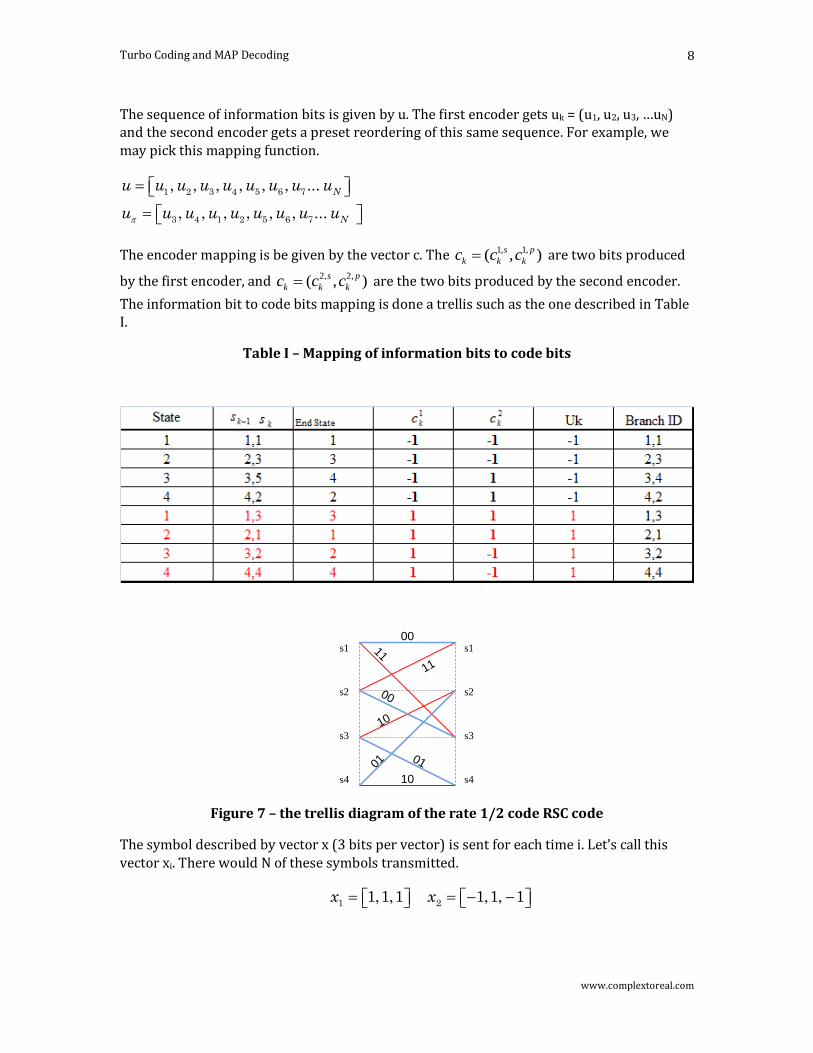
The sequence of information bits is given by u. The first encoder gets uk = (u1, u2, u3, …uN) and the second encoder gets a preset reordering of this same sequence. For example, we may pick this mapping function.

1 2 3 4 5 6 7

3 4 1 2 5 6 7

, , , , , , ...

, , , , , , ...

N

N

u u u u u u u u u

u u u u u u u u u

The encoder mapping is be given by the vector c. The 1, 1,( , ) s p

k k kc c c are two bits produced

by the first encoder, and 2, 2,( , ) s p

k k kc c c are the two bits produced by the second encoder.

The information bit to code bits mapping is done a trellis such as the one described in Table I.

Table I – Mapping of information bits to code bits

00

10

00

01

10

11

11

01

s1

s3

s2

s4

s1

s3

s2

s4

Figure 7 – the trellis diagram of the rate 1/2 code RSC code

The symbol described by vector x (3 bits per vector) is sent for each time i. Let’s call this vector xi. There would N of these symbols transmitted.

1 21,1,1 1,1, 1x x



9

1, 1, 2,( , , ) s p p

k k k ky y y y are the soft mapped bits. The goal is to take these and make a guess

about the transmitted x vector and hence code bits which inturn decode u, the information bit. Of this three soft bits, each decoder gets just two of these values. The first decoder

gets 1, 1,

1 ( , ) s p

k k ky y y and the second decoder gets 2, 2,

2 ( , ) s p

k k ky y y which are its respective

received data. Each decoder works with just two values. The second decoder however gets a reordered version of the systematic bit, so it is getting only one bit of independent information.

Log-likelihood Ratio (LLR)

Let’s take the information bit, a binary variable, uk, where u is its value at time k. Its Log-likelihood Ratio (LLR) is defined as the natural log of its base probabilities.

(ln( )

1)

( 1)k

k

k

P uL

Pu

u

(1.1)

If u has two values, +1 and -1 volts representing 0 and 1 bit and since these are equally likely, as they are in most communication system, then this ratio is equal to zero. This metric is used in most error correction coding and is called the log likelihood ratio or LLR. This is a sensitive metric, quite a bit better than a linear metric. Logs make it easy to deal with very small and very large numbers, as you well know.

Now note what happens to this metric, if the the binary variable is not equally likely, as happens in trellis decoding. From elementary probability theory, we know that sum of all probabilities of an event add to 1. So we can write that the probability of u = +1 as 1 minus the probability of u = -1.

( 1) 1 ( 1)k kP u P u

Now using equation (1.1), rewrite the expression of LLR from (1.2) as.

ln( 1)

1 ((

))

1

k

k

k

P uL

P uu

(1.2) is plotted in Figure 8 as a function of the probability of one of the events. Let’s say we are given L(uk) = 1.0. Then the probability that uk = +1 is equal to 0.73



10

-5

-4

-3

-2

-1

0

1

2

3

4

5

0 0.2 0.4 0.6 0.8 1

Probability, uk = +1

LL

R

Figure 8 – The range of LLR is from –∞ to +∞ and is a direct indication of the bit.

As we can see, if LLR, a non-dimensional metric, is positive, it is a pretty good indicator of the sign of the bit. This is an even better indicator than the Euclidean distance since its range is so large. LLR a very useful parameter and we will see how it is used in Turbo decoding.

In (1.2) formulate the LLR of a decoded bit uk, at time k, conditioned on the received signal, a sequence of N bits. The lower index of y means it starts at time 1 and the upper index means the ending point at N.

1

1

( 1| )( ) ln

( 1| )

Nk

k Nk

P u yL u

P u y

(1.2)

We can reformulate the numerator and denominator using Baye’s rule C.

1 1 1

1 1 1

( , 1) / ( ) ( , 1)( ) ln ln

( , 1) / ( ) ( , 1)

N N Nk k

k N N Nk k

P y u P y P y uL u

P y u P y P y u (1.3)

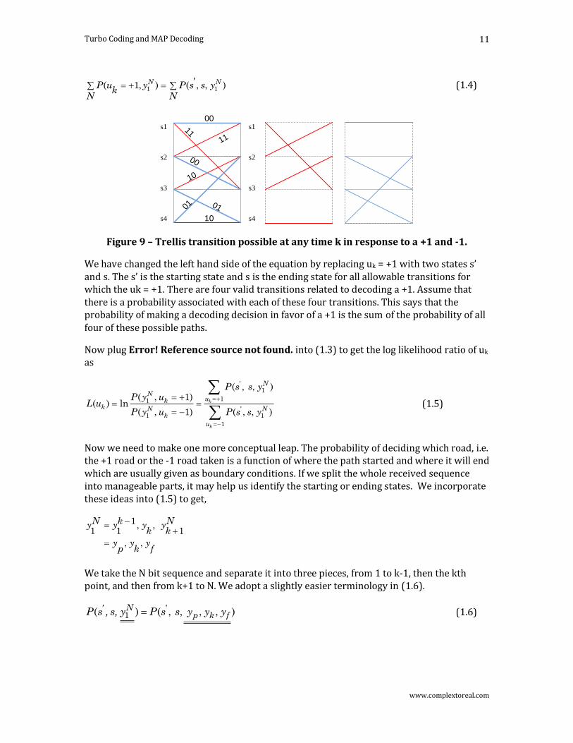
This formulation of the LLR includes joint probabilities between the received bits and the information bit, the numerator of which can be written as (1.4). For RSC trellis, each path is uniquely specified by any pair of these: 1. the start state s’, 2. the ending state s, 3. The input bit. If we know any two of these pieces of information, we can identify the correct path

without error. In this equation, we only know the whole sequence 1Ny , we do not know uk,

nor do we have any other of the piece of information. But what we do know is that saying a uk = 1 is same as saying that the correct path is one of the four possible paths shown in Fig. 8.

So the joint probability of 1( , 1) Nky u (having received the N bit sequence, the probability

of uk at time k = 1) is the same as replacing the information bit with ending and starting states. These formulations are equivalent.



11

1 1'( 1, ) ( , , )N NP u y P s s y

kN N

(1.4)

00

10

00

01

10

1111

01

s1

s3

s2

s4

s1

s3

s2

s4

Figure 9 – Trellis transition possible at any time k in response to a +1 and -1.

We have changed the left hand side of the equation by replacing uk = +1 with two states s’ and s. The s’ is the starting state and s is the ending state for all allowable transitions for which the uk = +1. There are four valid transitions related to decoding a +1. Assume that there is a probability associated with each of these four transitions. This says that the probability of making a decoding decision in favor of a +1 is the sum of the probability of all four of these possible paths.

Now plug Error! Reference source not found. into (1.3) to get the log likelihood ratio of uk as

'1

11

'1 1

1

( , , )( , 1)

( ) ln( , 1) ( , , )

k

k

N

Nuk

k N Nk

u

P s s yP y u

L uP y u P s s y

(1.5)

Now we need to make one more conceptual leap. The probability of deciding which road, i.e. the +1 road or the -1 road taken is a function of where the path started and where it will end which are usually given as boundary conditions. If we split the whole received sequence into manageable parts, it may help us identify the starting or ending states. We incorporate these ideas into (1.5) to get,

1, ,1 1 1

, ,

N k Ny y y yk k

y y yp k f

We take the N bit sequence and separate it into three pieces, from 1 to k-1, then the kth point, and then from k+1 to N. We adopt a slightly easier terminology in (1.6).

'1( ) ( , , , , )' N

p k fP s , s, y P s s y y y (1.6)



12

py The past sequence, the part that came before the current data point.

ky The current data point

fy The sequence points that come after the current point.

Rewrite using (1.6) using Baye’s rule of joint probabilities (D).

'

' '

( ) ( , , , , )

( | , , , ) ( , , , )

'

k fp

kp k pf

P s , s, y P s s y

P s s

y

y y

y

y y P s s y

(1.7)

This looks complicated but we are just applying Bayes rule to simplify (1.6) and to breakdown the terms in terms of past, present and future parts of the sequence. So that whenever we are making a decision about a bit +1 or a -1, a cumulative metric will take into account the starting and the ending point of the sequence. The starting and ending points of a convolutional sequence are known and we use this information to winnow out the likelier sequences.

The term fy is the future sequence and we make an assumption that it is independent of the

past and only depends on the present state s. We can remove these dependencies to simplify (1.7).

' '

'

( ) ( | , , , ) ( , , , )

( | ) ( , , , )

'

k kp

p

f

kf

pP s , s, y P s s y P s s yy y

ysyP s P s y

y (1.8)

Now apply Baye’s rule to the last term in (1.8), to get

' ' '( , , , ) ( , | , ) ( , )p k k p kP s s y y P s y s y P s y

' '( ) ( | ) ( , | , ) ( , )'

f k p pP s , s, y P y s P s y s y P s y (1.9)

Now define a few new terms.



13

'

1

'

( , )

( | )

( ', ) ( , | , )

(

(

'

)

)

k f

k

p

pc

k s yP s

P s

s s P s ys

y

y

s

(1.10)

The terms , , on the right are the metrics we will compute in MAP decoding. Now the numerator term of (1.5) becomes.

1( ) ( ) ( ',') )('

kk ksP s , s, y s ss (1.11)

We can plug this into (1.5) to get the LLR equation for MAP algorithm.

1

1

1

1

( ', )( )

( )( )

( ', )

( ')

( ')

k

k

k

u

k

k

k

k

u

k

k

s s

L

s

su

s

s

ss

(1.12)

1( ')

ks

This first term in (1.11) is called the Forward metric.

( )k s is called the Backward metric.

),'( ssk is called Transition metric.

The MAP algorithm allows us to compute these metrics. Decision is made at each time k, about the transmitted bit uk. Unlike Viterbi decoding where decision is made in favor if the likeliest sequence by carrying forward the sum of metrics, here the decision is made for the likeliest bit.

The MAP algorithm is also known as Forward-Backward Algorithm because we are assessing probabilities in both forward and backward time.

How to calculate the Forward metrics

We will start with the forward metric at time k.

'( ) ( , , , ) p k

All sta

k

tes

P ss s yy

Which is also equal to the probabilities at the previous state s’ times the transition probability to the current state s.



14

1'

'

'' (( ), ).( , ,) , )( All

k

s

k

All state

pk

s

s s sP s ss y y (1.13)

The initial condition is that since we always start at state 1,

0

1s if 1)(0

otherwise

s

Example:

s1

s3

s2

s4

k-1 k k+1

.2231

4.4817

4.4817

33.1155

.0302

1.6487

.6065

4.4817

(.9526)

(.0474)

0.2231

0

(0)

.0288

(.0063)

0(1) 1.0

0(2) 0

0(3) 0

0(4) 0

Figure 10 - Computing Forward metrics

The left most value at the top is the starting point, so it has a value of 0 (1) 1 , the starting

value of is = 0 at all the remaining three states. The ending forward metric at t = k is

' '1

'

( ) ( , ). ( )

(1) 1.4.4812 0 4.4812

(2) 1.0 4.4810.2 72 0.0 0.23 2311

k k

All s

k

k

s s s s

Notice that these numbers are larger than 1, which means, they are not probabilities but are called Metrics. It also means that since a typical Turbo code frame is thousands of trellis sections long that multiplication of these numbers may result in numerical overflow. For

that reason, both and are normalized.

Backward Metric ( )k s



15

Same as the initial values of 1)0(0 , we assume that since trellis always ends at state 1,

all probabilities at this point are equal to 1 or 0.

(1) 1N and zero elsewhere.

This probability is equal to the product of all transition probabilities times the probability at the last state working backwards.

' '1( ) ( ) ( , )

All s

k k s ss s (1.14)

Compare this with forward metric equation.

1

'

' '. ,) ( )( ( )k k

Alls

s ss s

s1

s3

s2

s4

k k+1 N

(.0033)

.0498

0

(0)

.0498

1.6487

.3679

.0821

.0821

.0005

(.001219)

20.085520.0855

(1.337)(1) 1.0N

(2) 0N

(3) 0N

(4) 0N

Figure 11 - Computing Backward metrics

' '1

2

2

20.0885

( ) ( ) ( , )

(1) 1.0 20.0885

(2) 1.0 0.049.0498 8

k k

Alls

k

k

s s s s

You can see these values at time k+1 for state 1 and 2. These are then normalized.



16

Numerical issues

In order to prevent data overflow that can happen in the very large trellis of a Turbo codes,,

)(sk and )'(1 sk need to be normalized. For forward metrics, we normalized them by

their sum.

( )( )

( )

kk

k

s

ss

s (1.15)

The reverse metric is similalry normalized by the same quantity as above. It s formulation looks different but it is the same thing as the term that normalized the forward metric. (Change index to k instead of k-1.)

1

1

2 1'

( ')( ')

( ') ( ', )k

k

k ks s

ss

s s s. (1.16)

How to calculate transition probabilities

Computing transition metrics turns out to be the hardest part. To restate the definition of the transition metric from (1.10)

'( ', ) ( , | , )k pcs s P s y s y

The transition itself does not depend on the past, so we can remove the dependency on the past and then apply the Baye’s theorem.

'( ', ) ( , | , k k ps s P s y ys

'

' '

)

( , | )

( | , ) . ( | )

k

k

P s y s

P y s s P s s

(1.17)

'( ', ) ( | , ) . ( ) k k ks s P y s s P u (1.18)

There are two terms in this final definition of the transition metric. Let’s take the last one first. Here P(uk) is a-priori probability of the input bit. Let’s take its log likelihood.

( 1) ( 1)( ) log log

( 1) 1 ( 1)

k kk

k k

P u P uL u

P u P u

Or by taking this expression to power of e, we get



17

( ) ( 1)

1 ( 1)kL u k

k

P ue

P u

From here, some clever algebra gives us

( )

( )

( )

( )

( )/2( )/2

( )

( 1) (1 ( 1))

1

1

1

1

k

k

k

k

k

k

k

L u

k k

L u

L u

L u

L uL u

L u

P u e P u

e

e

e

ee

e

Now we get the general expression for both, +1 and -1.

2/)(

)(

2/)(

1)1( k

k

k

uL

uL

uL

k ee

euP

(1.19)

The term underlined is a common factor and designated by

( )/2

( )1

k

k

L u

k L u

eA

e

The a-priori probability is now given by

( )/2( 1) kL uk kP u A e

(1.20)

Now for the second term in transition metric expression of (1.18), ),|( ' ssyP k can be

written as

'

1

( | , ) ( | ) ( | )n

k k k kl kl

l

P y s s P y c P y c

For rate ½, we can write this simply as,

1, 1 1, 2( | ) s p

k k k k k kP y x y c y c

This is just a correlation of the input signal values with the trellis values, c. The received signal values yk are assumed to be corrupted by an AWGN process. The probability

P( | )kl kly c is given in a Gaussian channel by



18

2

2

1 1( | ) exp ( )

22

kl kl kl klP y c y c (1.21)

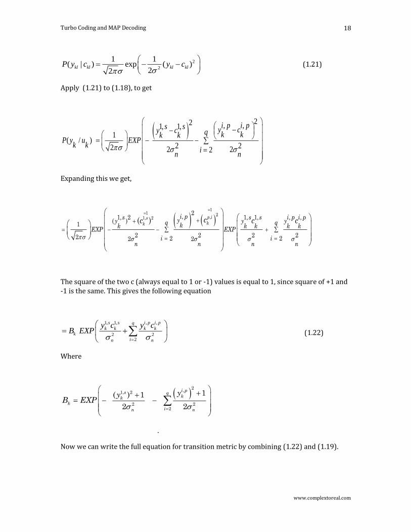
Apply (1.21) to (1.18), to get

22 , ,1, 1,

1( / )

2 22 2 22

i p i ps s y cy c q k kk kP y u EXP

k ki

n n

Expanding this we get,

1

1 2,1, 2

2, , ,1, 2 1, 1,

( )1

2 2 2 22 2 22 2

( )p iskk

i p i p i ps s syy y yq qkk k k k kEXP EXP

i in n n n

cc c c

The square of the two c (always equal to 1 or -1) values is equal to 1, since square of +1 and -1 is the same. This gives the following equation

1, 1, , ,

2 22

s s i p i pq

k k k k

k

in n

y c y cB EXP (1.22)

Where

2

,1, 2

2 22

1( ) 1

2 2

i ps qkk

kin n

yyB EXP

.

Now we can write the full equation for transition metric by combining (1.22) and (1.19).



19

'( ', ) ( | , ) . ( ) k k ks s P y s s P u .

, ,1, 1,( ) / 2

exp2 2

2

i p i ps sqy c y c L c

k k k k kB A ek k

in n

(1.23)

Ak and Bk are constants and are not important because when we put this expression in the LLR form, they will cancel out. The index q = 2 for rate ½ code we are using for example.

Now we define,

2 0

0 0

2 2 / 2 /

cn

b b

N E p

coderate E N E N (1.24)

Where p is inverse of code rate, i.e. equal to 2 for code rate = 1/2

0 0

b cE E

N rate N

. (1.25)

where 0

bE

N is ratio of the un-coded bit energy to noise PSD, Ec is coded bit energy, and Ec=

code rate Eb.

Substitute for 2

02 /

n

b

p

E N into (1.23) we have

1, 1 ,1 10

2

4 / 1exp ( )

2 2 2

s i p iq

b k k k kk k k k

i

E N y c y cA B L c c

p



20

1, 1 , 1 10

2

4 / 1 1exp ( )

2 2

qs i p ib

k k k k k k k k

i

E NA B y c y c L c c

p

1 1 1, 1 ,0 0

2

4 / 4 /1 1 1exp ( ) exp

2 2 2

qs i p ib b

k k k k k k k k

i

E N E NA B L c c y c y x

p p

With 00

4 /4. /

b

c s

E NL E N

p

1 1 1, 1 ,

2

1 1 1exp ( ) exp

2 2 2

qs i p i

k k k k k k k k

i

A B L c c Lc y c Lc y c (1.26)

where we define a new partial transition metric, the underlined part of (1.26).

e ,

2

1 ( ', ) exp

2

qi p i

k k

i

s s Lc y c .

In summary the LLR of the information bit uk at time k is,

)(~

),'()'(~

)(~

),'()'(~

log)(1

1

ssss

ssss

uLkk

u

k

kk

u

k

k

(1.27)

s s

kk

s

kk

ksss

sss

s

'

1

'

1

),'()'(~

),'()'(~

)(~

, 0

1s if 1)(~

0

otherwise

s (1.28)



21

s s

kk

s

kk

ksss

sss

s

'

12

1),'()'(~

),'()(~

)'(~

, 0

1s if 1)(

~

otherwise

sN (1.29)

1 1 1, 1 ,

2

1 1 1( ', ) exp ( ) exp

2 2 2

qe s i p i

k k k k k k

i

s s L c c Lc y c Lc y c (1.30)

Substitute (1.30) into (1.27), to get

q

i

i

k

pi

kk

s

kkk

e

k

u

k

q

i

i

k

pi

kk

s

kkk

e

k

u

k

cyLccyLcccLss

cyLccyLcccLss

2

,1,111

1

2

,1,111

1

2

1exp

2

1)(

2

1exp)(

~)'(~

2

1exp

2

1)(

2

1exp)(

~)'(~

log

(1.31)

If q = 2, the equation become

1 1 1, 1 2, 2

1

1 1 1, 1 2, 2

1

1 1 1( ') ( ) exp ( ) exp

2 2 2log

1 1 1( ') ( ) exp ( ) exp

2 2 2

e s p

k k k k k k k k

u

e s p

k k k k k k k k

u

s s L c c Lc y c Lc y c

s s L c c Lc y c Lc y c

1 1,( ) s

k kL u and Lc y can be pulled out because both numerator and denominator are constant.

The factor ½ and 1

kc cancel. We get,

1

1 1,

1

( ') ( ) ( ', )

( ) ( ) log( ') ( ) ( ', )

e

k k k

s u

k k k e

k k k

u

s s s s

L u L c Lc ys s s s

Where



22

e ,

2

1( ', ) exp

2

qi p i

k k

i

s s Lc y c

This equation can be broken into three distinct numbers. They are

extrinsicLchannelLaprioriL ___ (1.32)

1( )k

L c is the a-priori information about uk, s

kyLc ,1 is the channel value calculated from the

knowledge of the SNR and the received signal. The third term is called the a-posteriori term, also called the extrinsic L value.

),'()(~

)'(~

),'()(~

)'(~

log_1

1

ssss

ssss

extrinsicLe

kk

u

k

e

kk

u

k

(1.33)

During each iteration the decoder produces the extrinsic value using the first two numbers as input. The extrinsic value it produces becomes the input to the next decoder.

)()()( 1

12

1

21

,11

1 k

e

k

es

kk cLcLyLccL ,

And eventually a decision is made about the bit in question by looking at the sign of the L value.

})(sign{L~ 1

1 kk cu ,

The process can continue until the extrinsic values stop changing with a preset threshold. Or the algorithm can allow just a fixed number of iterations.

DEC1 DEC2

Extrinsic L

value from

1 to 2

1

1,sy

1, py

2,sy

2, py

Extrinsic L

value

from 2 to 1

Figure 12 – Iterative nature of Turbo decoding.



23

So that’s about it. I hope it was helpful. The next tutorial goes through the MAP algorithm in a step-by-step example.

Please contact me if you find errors.

Charan Langton www.complextoreal.com

Copyright, 2006, 2007 Charan Langton All Rights reserved

http://www.complextoreal.com/



24

References

[1] Turbo code in IS-2000 Division Multiple-Access Communications Under Fading By Jian Qi. Masters Thesis, Wichita State University, Fall 1999. Comment: Available on the Internet. I used Ms. Qi’s terminology and heavily relied on this work. Its an excellent reference.

[2] http://www.iep.utm.edu/a/apriori.htm, "A Priori and A Posteriori" - an article by Jason Baehr in the Internet Encyclopedia of Philosophy.

[3] http://www.lockergnome.com/it/2007/06/13/a-priori-statistics-to-a-posteriori-probability/

[4] Not complete…

http://www.iep.utm.edu/a/apriori.htm

http://www.iep.utm.edu/a/apriori.htm

turbo coding and map decoding - part 1 - complex to...

Documents