an analogue of the kp theory in dimension 2

History: 1-dimensional KP theory An analogue of the KP theory in dimension 2

An analogue of the KP theory in dimension 2

A.Zheglov1

1Moscow State University, Russia

XVII Geometrical Seminar, Zlatibor, Serbia, September 3-8,2012


Outline

1 History: 1-dimensional KP theoryIsospectral deformations of ordinary differential operatorsSato GrassmanianGeometric solutionsExamples

2 An analogue of the KP theory in dimension 2Isospectral deformations of partial differential operatorsQuasi elliptic ringsSchur pairsGeometric dataExamples


Isospectral deformations of ordinary differential operators

The Kadomtsev-Petviashvili (KP) equation

The Kadomtsev-Petviashvili (KP) equation is a non-linearpartial differential equation:

(4ut − u′′′ − 12uu′)′ = 3uyy for u(t , x , y).

It was found by Kadomtsev and Petviashvili in 1970, and themotivation for introducing it was to study transversal stability ofthe soliton solutions of the famous Korteveg and de Vries (KdV)equation

4ut − u′′′ − 12uu′ = 0 for u(t , x).

The KdV equation was derived in 1895 from the Navier-Stokesequation of fluid dynamics as a special limit to give a model ofnonlinear wave motions of shallow water observed in a canal.



The Kadomtsev-Petviashvili (KP) equation

It is one of the most interesting non-linear PDE, because

1 There is a rich theory connecting this equation with manyother famous equations as well as with different problemsin various branches of mathematics

2 There are many exact solutions of this equation

Below is a brief explanation of the KP theory.



A general ring of pseudo-differential operators

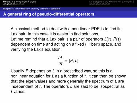
A classical method to deal with a non-linear PDE is to find itsLax pair. In this case it is easier to find solutions.Let me remind that a Lax pair is a pair of operators L(t),P(t)dependent on time and acting on a fixed (Hilbert) space, andverifying the Lax’s equation:

∂L∂t

= [P,L].

Usually P depends on L in a prescribed way, so this is anonlinear equation for L as a function of t . It can then be shownthat the eigenvalues and more generally the spectrum of L areindependent of t . The operators L are said to be isospectral ast varies.




In the case of the KP equation one can proceed as follows.

Definition

We say {P(t)|t ∈ M}, where M is an open domain of CN , is afamily of isospectral deformations if there exist ordinarydifferential operators Q1(t),Q2(t), . . . ,QN(t) depending on theparameter t ∈ M analytically such that the following system ofequations has a nontrivial solution ψ(x , t ;λ) for everyeigenvalue λ of P(t):

P(t)ψ(x , t ;λ) = λψ(x , t ;λ)∂∂t1ψ(x , t ;λ) = Q1(t)ψ(x , t ;λ)

. . .∂∂tNψ(x , t ;λ) = QN(t)ψ(x , t ;λ)

(1)



A general ring of pseudo-differential operators

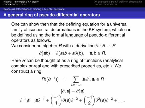
One can show then that the defining equation for a universalfamily of isospectral deformations is the KP system, which canbe defined using the formal language of pseudo-differentialoperators as follows.We consider an algebra R with a derivation ∂ : R → R

∂(ab) = ∂(a)b + a∂(b), a,b ∈ R.

Here R can be thought of as a ring of functions (analyticalcomplex or real and with prescribed properties, etc.). Weconstruct a ring

R((∂−1)) :∑

i�+∞ai∂

i ,ai ∈ R

[∂,a] = ∂(a)

∂−1a = a∂−1 +

(−11

)∂(a)∂−2 +

(−12

)∂2(a)∂−3 + . . . ,



A ring of pseudo-differential operators in one variable:decomposition

where (ik

)=

i(i − 1) . . . (i − k + 1)k(k − 1) . . . 1

, if k > 0.

Let’s consider for simplicity the ring R = C[[x ]] with usualderivation ∂(x) = 1. We add infinite number of formal variables:t1, t2, . . .. There is a unique decomposition in the ringE = R[[t1, t2, . . .]]((∂−1)):

if A ∈ E , then A = A+ + A−,

where A+ ∈ R[[t1, t2, . . .]][∂], A− ∈ R[[t1, t2, . . .]][[∂−1]] · ∂−1.



KP-hierarchy

Let L ∈ R[[t1, t2, . . .]]((∂−1)) be of the following type:

L = ∂ + u1∂−1 + u2∂

−2 + . . . , ui ∈ R[[t1, t2, . . .]].

DefinitionThe classical KP-hierarchy is the following infinite system ofequations (a generalized Lax equation):

∂L∂tn

= [(Ln)+,L], n ∈ N.



Partial equations of the KP-hierarchy: KP and KdV equations

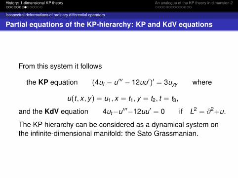
From this system it follows

the KP equation (4ut − u′′′ − 12uu′)′ = 3uyy where

u(t , x , y) = u1, x = t1, y = t2, t = t3,

and the KdV equation 4ut−u′′′−12uu′ = 0 if L2 = ∂2+u.

The KP hierarchy can be considered as a dynamical system onthe infinite-dimensional manifold: the Sato Grassmanian.


Sato Grassmanian

Sato Grassmanian

DefinitionA C-subspace W in C((u)) is called a Fredholm subspace if

dimC W ∩ C[[u]] <∞ and dimCC((u))

W + C[[u]]<∞.

RemarkOne the set of Fredholm subspaces of C((u)) one can definethe structure of infinite-dimensional projective algebraic variety,the Sato Grassmanian Gr(C((u))).Since W ⊂ C((u)), we can consider the stabilizer subringA ⊂ C((u)): A ·W ⊂W . We define its rank

rankA = GCD{νu(a)|a ∈ A},

where νu is a discrete valuation on the field C((u)).


Geometric solutions

Geometric solutions of the KP-hierarchy

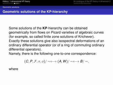
Some solutions of the KP-hierarchy can be obtainedgeometrically from flows on Picard varieties of algebraic curves(for example, so called finite zone solutions of Krichever).Exactly these solutions give also isospectral deformations of anordinary differential operator (or of a ring of commuting ordinarydifferential operators).Namely, there is the following one-to-one correspondence:

(C,P,F , π, φ)/ ∼←→ (A,W )/ ∼←→ B/ ∼,

where


Geometric solutions

Definitions

DefinitionB ⊂ D is a commutative C-subalgebra, which is elliptic, i.e. Bhas a monic element P of order greater than zero.For an elliptic commutative subalgebra B ⊂ D we define

rankB = GCD{ord Q|Q ∈ B}.

B1 ∼ B2 if there is an invertible element f ∈ R∗ such that

B1 = fB2f−1.


Geometric solutions

Schur pairs and geometric data

Definition

We call (C,P,F , π, φ) a geometric data of rank r if it consists ofthe following data:

C is a reduced irreducible projective curve over C;

P ∈ C is a regular on C closed point;

π : OP −→ k [[u]] is a ring homomorphism such thatν(π(f )) = r , where f ∈ OP is a local equation of the point P.

F is a torsion free coherent sheaf on X of rank r satisfying

H0(C,F) = H1(C,F) = 0.

φ : FP ' k [[u]] (a trivialization of F at P)


Geometric solutions

Schur pairs

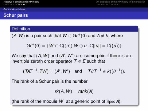
Definition(A,W ) is a pair such that W ∈ Gr+(0) and A 6= k , where

Gr+(0) = {W ⊂ C((u))|W ⊕ u · C[[u]] = C((u))}

We say that (A,W ) and (A′,W ′) are isomorphic if there is aninvertible zeroth order operator T ∈ E such that

(TAT−1,TW ) = (A′,W ′) and T∂T−1 ∈ k((∂−1)).

The rank of a Schur pair is the number

rk(A,W ) = rank(A)

(the rank of the module W at a generic point of Spec A).


Examples

Examples of KdV solutions

ExampleIf we take the pair

W = 〈1 + t , t−i , i ≥ 1〉 A = k [t−2, t−3] :

then the corresponding ring B is the old known example ofBurchnall and Chaundy

P = ∂2x − 2x−2, Q = ∂3

x − 3x−2∂x − 3x−3

and the corresponding curve is the rational cuspidal curve.The solution of the KdV equation with the initial conditioncorresponding to this data is the famous rational solution

u(x) = (x−1)x .


Isospectral deformations of partial differential operators

We can try to repeat the definition of isospectral deformationsalso in the case of partial differential operators. But now, if wewill try to proceed the arguments from one dimensional caseand derive a defining equation for a universal family ofisospectral deformations, we will come to a necessity1) to normalize in certain sense the operators2) to take a completion of the ring of partial differentialoperators.After that we really can proceed and get the defining equation— a modified Parshin’s KP system.Below are the exact definitions.



Definitions

DefinitionLet R = C[[x1, x2]], denote by M = (x1, x2) the maximal ideal.Then define the ring

D1 = {a =∑q≥0

aq∂q1 |aq ∈ C[[x1, x2]]

and for any N ∈ N there exists n ∈ N such thatordM(am) > N for any m ≥ n}. (2)

DefineD = D1[∂2] ⊃ D = R[∂1, ∂2].



Definitions

DefinitionDefine

E = D1((∂−12 )) ⊃ D ⊃ D.

This is an associative ring of formal pseudo-differentialoperators. Denote by E (−1) the algebra D1[[∂

−12 ]]∂−1

2 . We havea natural direct sum decomposition

E = D ⊕ E (−1)

as a module.



Generalization of the KP-hierarchy in dimension 2

Definition

We consider L,M ∈ E [[{tk}]] such that

L = ∂1 + u1∂−12 + . . . , M = ∂2 + v1∂

−12 + . . . ,

where ui , vi ∈ D1[[{tk}]].

Let N = (L,M) and [L,M] = 0, then hierarchy is

∂N∂tk

= V kN ,

where V kN = ([(LiM j)+,L], [(LiM j)+,M]),

k = (i , j) ∈ Z+ × Z+.


Quasi elliptic rings

Definitions

Definition

The ring B ⊂ D of commuting operators is called quasi elliptic ifit contains two monic operators P,Q such that

ordΓ(P) = (0, k) and ordΓ(Q) = (1, l)

for some k , l ∈ Z, where we say that an operator P ∈ E+ hasorder ordΓ(P) = (k , l) if

P =l∑

s=−∞ps∂

s2,

where ps ∈ D1, pl ∈ k [[x1, x2]][∂1] = D1, and ord(pl) = k .


Schur pairs

Schur pairs

Definition

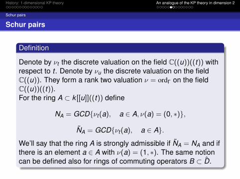
Denote by νt the discrete valuation on the field C((u))((t)) withrespect to t . Denote by νu the discrete valuation on the fieldC((u)). They form a rank two valuation ν = ordΓ on the fieldC((u))((t)).For the ring A ⊂ k [[u]]((t)) define

NA = GCD{νt(a), a ∈ A, ν(a) = (0, ∗)},

NA = GCD{νt(a), a ∈ A}.

We’ll say that the ring A is strongly admissible if NA = NA and ifthere is an element a ∈ A with ν(a) = (1, ∗). The same notioncan be defined also for rings of commuting operators B ⊂ D.


Schur pairs

Schur pairs

Definition

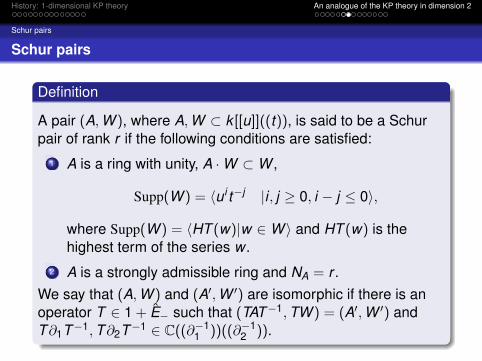
A pair (A,W ), where A,W ⊂ k [[u]]((t)), is said to be a Schurpair of rank r if the following conditions are satisfied:

1 A is a ring with unity, A ·W ⊂W ,

Supp(W ) = 〈ui t−j |i , j ≥ 0, i − j ≤ 0〉,

where Supp(W ) = 〈HT (w)|w ∈W 〉 and HT (w) is thehighest term of the series w .

2 A is a strongly admissible ring and NA = r .We say that (A,W ) and (A′,W ′) are isomorphic if there is anoperator T ∈ 1 + E− such that (TAT−1,TW ) = (A′,W ′) andT∂1T−1,T∂2T−1 ∈ C((∂−1

1 ))((∂−12 )).


Geometric data

Geometric data

Definition

We call (X ,C,P,F , π, φ) a geometric data of rank r if it consistsof the following data:

X is a reduced irreducible projective algebraic surfacedefined over a field C;

C is a reduced irreducible ample Q-Cartier divisor on X ;

P ∈ C is a regular on C and on X closed point;

π : OP −→ k [[u, t ]] is a ring homomorphism such thatν(π(f )) = (0, r), ν(π(g)) = (1,0), where f ∈ OP is a localequation of the curve C in a neighbourhood of P, andg ∈ OP restricted to C is a local equation of the point P onC.


Geometric data

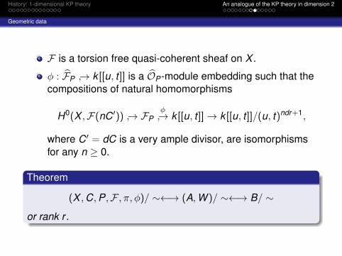
F is a torsion free quasi-coherent sheaf on X .

φ : FP ↪→ k [[u, t ]] is a OP-module embedding such that thecompositions of natural homomorphisms

H0(X ,F(nC′)) ↪→ FPφ↪→ k [[u, t ]]→ k [[u, t ]]/(u, t)ndr+1,

where C′ = dC is a very ample divisor, are isomorphismsfor any n ≥ 0.

Theorem

(X ,C,P,F , π, φ)/ ∼←→ (A,W )/ ∼←→ B/ ∼

or rank r .


Examples

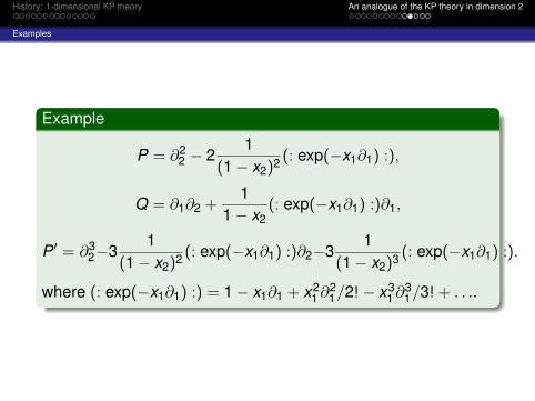
Example

Example

Let’s give one example of a pair of commuting operators in thering D connected with one of the simplest points from theanalogue of the Sato Grassmanian.Let’s take a subspace

W = 〈1 + t , t−iuj , i ≥ 1,0 ≤ j ≤ i〉 ⊂ C[[u]]((t)).

One can easily check that its ring of stabilizers containselements t−2, t−3,ut−2. The maximal ring of stabilizers will beinfinitely generated over C.The Schur pair (W ,A) with a finitely generated ring Acontaining the elements above corresponds to a geometricdata with a surface being singular toric surface.


Examples

Example

P = ∂22 − 2

1(1− x2)2 (: exp(−x1∂1) :),

Q = ∂1∂2 +1

1− x2(: exp(−x1∂1) :)∂1,

P ′ = ∂32−3

1(1− x2)2 (: exp(−x1∂1) :)∂2−3

1(1− x2)3 (: exp(−x1∂1) :).

where (: exp(−x1∂1) :) = 1− x1∂1 + x21∂

21/2!− x3

1∂31/3! + . . ..


Examples

Equations

ExampleIf we derive equations of isospectral deformations of theoperators above, we obtain the following equations:

∂s1

∂t1=

14(s1)x2x2x2−

32(s1)

2x2,

∂s1

∂t2= −(s1)x2(s1)x1−

12(s1)x2x2∂1,

(3)∂s1

∂t3= −(s1)

2x1− (s1)x1x2∂1 − (s1)x2∂

21 ,

where s1(x1, x2, t1, t2, t3) = s1(t) is the first coefficient of theoperator S(t) = 1 + s1(t)∂−1

2 + . . ., and S(0) = S is theconjugating operator: P = S∂2

2S−1.


Examples

Notably

s1(0) =1

1− x2(: exp(−x1∂1) :)

is a solution of the equations above. This corresponds to thefollowing fact from one-dimensional KP theory: the functionu(x) = (x−1)x is the rational solution of the KdV equation (andthis function is the halved coefficient of the operator P inexample below).


Examples

Final remark

A simple analysis of equations above show that even if we startwith a commutative ring of partial differential operators (whatmeans that s1(0) ∈ k [[x1, x2]][∂1] = D1), the isospectraldeformations will not be partial differential operators, butoperators in D, since s1(t) /∈ D1 for general t .This situation is similar to the problem of describingcommutative rings of ordinary differential operators withpolynomial coefficients in dimension one. In one dimensionalKP theory, if we start with a commutative ring of ordinarydifferential operators with polynomial coefficients, its isospectraldeformations (which are connected with solutions of the KPequation) will consist of operators with not polynomialcoefficients though they will still be ordinary differentialoperators.

an analogue of the kp theory in dimension 2

Documents