an accurate heston implementation with usd-cop data

T

AN ACCURATE HESTON IMPLEMENTATION WITH

USD-COP DATA

Javier Jaher Alfonso Lázaro Salcedo

Universidad de l Rosario

Facultad Economıa

Bogota, Colombia

2018

AN ACCURATE HESTON IMPLEMENTATION WITHUSD-COP DATA

JAVIER JAHER ALFONSO LAZARO SALCEDOADVISOR: RAFAEL SERRANO

These words are dedicated specially to the memory of my dad, and to my mom,who never stop believing in me.

Abstract. This study find by empirical evidence a fast and accu-rate way to calculate the price of a European Call using the Heston(1993) model.

It calculate and uses a benchmark price calculated with the men-tioned Heston 1993 pricing approaches and the trapezoidal rulewith a = 1e-20000; b = 300; N = 10000000, to find which com-bination of Heston pricing process and numerical schems leads toa computationally faster and more accurate price process. Twoequivalent pricing methods and seven numerical schemes are cal-culated in order to find wich combination take less time to becompute and is closes to the benchmark as posible. The studyuses Q-measure in the sense of spot data, and the other P-measurein the sense of historical data. That mean the study calculatetwo parameter sets. one under mesure Q and other under P byMaximum Likelihood and non-linear least square function, respec-tively, to somehow proof the conclution dose not depents on howthe parameter are found. Study stands that the accuraste wayto calculate the Heston price in the Colombian FX market dataused is consolidating the integrals for the probability P1 and P2that the original framework propose and solve the integral usingGauss-Legendre or Gauss-Laguerre.

Date: February 15, 2018.2010 Mathematics Subject Classification. 65D30.Key words and phrases. Heston model, USD-COP, Fourier pricing, Fourier trans-

formation,Fundamental transform, Damping factor,Quantitative methods, Gauss-ian cuadrature, Newton cotes.

Thanks to Dana. In the distance you gave me strength. Special thanks to mycousin Dasaed for the patience that he has always had with my English. Hope thissentence is grammatically okay Dasa.

1

2 JAVIER LAZARO

1. Introduction

In developed markets, the Heston model and a wide variety of morecomplex models have been implemented to make better and accu-rate valuations of options so that affordable Hedging Strategies canbe made. The drawback of these models is that the advantage of amore realistic modeling of the variance can be offset by the costs ofcalibration and implementation due to the fact that closed-form for-mulas are rarely available like in BSM (Black-Scholes-Merton) model.See [GT11].

In an emerging market such as the one in Colombia, those morecomplex models are implemented by a few as a result of the marketliquidity. In other words, if the profit of use de profit of selling optionsat the Heston price in a hedge strategy is not atractive to investors, themarket hardly will improve the liquidity. Investors should have incen-tives to move their money from colombian equities and fixed incometo the derivatives market. The reader may find usedfull the process offinding the price of an european call option in the Colombian FX mar-ket computationally faster and accurate so a better replicating portfoliocan be used.

In order to achive the goal, the study shows how to implement theHeston model, a more complex model than BSM , with two equivalentapproaches and seven different numerical schemes to find wich combi-nation leads to a more computationally faster and accurate valuationof call options in the Colombian FX market. Think about to equivalent”formulas” that have one or two integrals, and in order to solve them,the study present sevent diferent ways to do it.

The to equivalent pricing approaches or ”formulas” are (i) the Hes-tons original paper and its Characteristic function, (ii) Consolidatingthe integrals for the probability P1 and P2 that the original frameworkpropose. In the Apendix, the interest reader can found other evivalentpricing method

Diferent ways to solve the integral are presented and each of themare called numerical scheme. The first four are Newton Cotes formulas(i)Mid-Point (ii) Trapezoidal rule, (iii) Simpson’s rule, (iv) Simpson’s3/8 rule. The remaining schemes are Gaussian Cuadratures: (v) Gauss-Laguerre, (vi) Gauss-Legendre, (vii) Gauss-Lobato.

AN ACCURATE HESTON IMPLEMENTATION 3

Furthermore, this study calculate de price under the mesure Q and Pto show in some way that the conclusion does not depend on the mea-sure used. In order to do that, the paremeter set Θ = {κ, θ, σ, v0, ρ} isestimated by Maximum Likelihood (hereafter MLE)[AW09] under therisk neutral mesure Q and also by calibration using a non-linear leastsquare function (hearafter NLLS) under mesure P . The study will gointo this topic later.

Evenmore, in one hand, to find the accurate solution, the study cal-culate a benchmark price that have at least 41 decimal1 and compare allprices with those in order to find which combination of price approachand numerical scheme have the smallest error. In the other, to find thecomputationally faster price approach and numerical scheme the timethe code took to calculate de price is averaged and compere. How thebenchmark is calculated and chosen will be explained in chapter 9.

The data used in this study was chosen in a trading session with-out high impact of political or macronomic news that could afected theprice of the underlying. Likewise, the correlated currencies did not havesudden movements compared with the dollar. The data used in thisstudy was from July 12, 2016. This day opened at 2,935 COP/USDand closed at 2,918 COP/USD.

Figure 1. Market Data Used

Finally, this study uses Rouag book [RH13] as a detailed guide. Themathematical formulas for the pricing calculation as well as a big partof the code were heavily supported on his book. Thanks to his awesome

1To fulfill the study goal, it will be assumed that the level of acurracy of thebencjmark will absolute because it is going to be the initial assumption to find themost accurate price

4 JAVIER LAZARO

work this study is possiblee

1.1. How is the Study Organized. The study is composed of eigthchapters. The first one is the already mentioned introduction. Thesecond one focuses on the theoretical framework and the approaches.Chapter three is oriented to the numerical schemes that solved the re-maining integral. The FX Market Conventions are explain in chapterfour In chapter five and six the estimation and calibration topic is cov-ered respectively. Chapter seven checks how the benchmark is defined.Chapter eigth proofs wich pricing approach has the fastest numericalscheme with the most accuracy. Chapter nine ilustrated how the studyfind the most accurate method. Chapter ten ilustrate how the accu-rate method and faster scheme are used to reach the conclusion of thestudy. Finally, chapter eigth presents the conclusions.

2. The Heston Model

This chapter presents the original Heston framework and introducesthe reader to other six equivalent pricing approaches, presented in theorder they where published.

2.1. Heston 1993. The Heston (1993) models the underling with twoSDE, one for the price, St and one for the variance vt.

(2.1.1)dSt = µStdt +

√vtStdW1,t

dvt = κ(θ − vt)dt + σ√vtdW2,t)

EP [dW1,t dW2,t] = ρdt

Where:

(2.1.2)

µ drift process of the underling,κ > 0 mean reversion speed of the variance,θ > 0 mean reversion level of thevariance,σ > 0 volatility of volatility,v0 > 0 initial level of volatility,

λ volatility risk parameter.

Hence, the model is constituted by a bivariate system of SDE whereW1,t has a correlation ρ ∈ [−1 1] with W2,t and is expected to be pos-itive in the USD-COP FX market since investors seek shelter in the


strongest foreign exchange when vt increases. The correlation param-eter, ρ, controls the skewness of the density of the logarithm of theunderlying, when its positive the probability density will be positiveskewed.

Under the risk neutral mesure Q the model stand:

(2.1.3)dSt = rStdt +

√vtStdW1,t

dvt = [κ(θ − vt)− λSt,vt,t]dt + σ√vtdW2,t)

where W is the Brownian motions under the risk-neutral process,λSt,vt,t is the the volatility risk parameter. λ 2, is set to zero because itis embedded into κ∗ and θ∗:

(2.1.4)

λSt,vt,t = λv

dSt = rStdt +√vtStdW1,t

dvt = κ∗(θ∗ − vt)dt + σ√vtdW2,t)

EQ[dW1,t dW2,t] = ρdt

where κ∗ = κ+ λ and θ∗ = κθκ+λ

When estimating the risk-neutral parameters. For notation simplic-ity the asterisk will be drop and it will be understood hereafter thatthe study is dealing with the risk-neutral measure.

The characteristic function (hereafter CF) approach to option pricingof Heston 1993 can be applied to the characterization of call prices inthe form of discounting the expected value of the payoff function underthe risk-neutral measure as:

(2.1.5)

C(k) = e−rdτEQ[(St −K)+]

= e−rdτEQ[(St −K)1St>K ]

= e−rdτEQ[St1St>K ]−Ke−rdτEQ[1St>K ]

= Ste−rf τP1 − Ke−rdτP2

where the quantities P1 and P2 represent the probability of the op-tion expiring ITM conditional on the filtration, Ft, under the measureQ. In other words P1 uses the underlaying as numerarie while P2 uses

2 Estimation of λ is subject-matter to its own research. See Bollerslev et all.(2011)[BGZ11]

6 JAVIER LAZARO

the bond, Bt. Bakshi and Madan (2000)[BM00] prove that the deriva-tion of the call price under change of numerarie is valid for the BSMand Heston model.

In the BSM world, P1 = φ(d1) and P2 = φ(d2) are calculatedstraightforward, on the other hand, for the Heston model to obtainsuch probabilities the inversion theorem of the CF of Gil-Pelaez (1951)[GP51] must take place. For details on pricing with CF see Zhu (2009)[Zhu09]. To implement the inversion theorem, the CF must be known.Heston (1993) proposes the following CF:

(2.1.6) fj(φ;xt, vt) = exp( Cj(τ, φ) + Dj(τ, φ)vt + iφxt)

for j = 1, 2. Heston (1993) stands that the CF for the log-returns,xT = lnSt, is a way to exploit the linearity coefficient on the modelPDE (Partial Differential Equation). The calculation of the HestonPDE is slightly more difficult than BSM PDE. The interested readercan follow up the derivation in Rouah (2013) to get:

(2.1.7)

∂Pj∂j

+ ρσv∂2Pj∂v∂x

+1

2v∂2Pj∂x2

+1

2σ2v

∂2Pj∂v2

+ (r + µjv)∂Pj∂x

+ (a− bjv)∂Pj∂v

= 0.

where µ1 = 12, µ2 = −1

2, a = κθ, b1 = κ+ λ− ρσ, b2 = κ+ λ. The CF

will follow the PDE (2.1.7) as a consequence of the Feyman-Kac the-orem that stipulates the solution f(φ;xt, vt) = E[ei φ lnSt |xt, vt], whichis the CF for XT = lnSt. Once it is known that the PDE (2.1.7) canbe applied to the CF, one may proceed.

To find the coefficients of the CF (2.1.6) one must express the PDE(2.1.7) for the CF3, express the six partial derivate of the new PDE interms of the solution proposed by Heston (1993) (2.1.6), replace in thenew PDE, solve the remaining Riccati equation Dj and the ordinarydifferential equation Cj in order to get:

(2.1.8)

Dj(τ, φ) =bj − ρσiφ+ dj

σ2

(1− edjτ

1− gjedjτ

),

Cj(τ, φ) = riφτ +a

b

[(bj − ρσiφ+ dj)τ − 2ln

(1− gjedjτ

1− gj

)],

3change Pj for fj


where gj =bj−ρσiφ+djbj−ρσiφ−dj , dj =

√(ρσiφ− bj)2 − σ2(2µjiφ− φ2) for

j=1,2.

Note that the CF does not depend on the strike, but it does on thematurity, τ . This implies, when computing the Non-linear least squarefunction for calibration purposes, the values for f1(φ) and f2(φ) canbe calculated only once for each maturity and must be used repeatedlyacross the deltas.4 This method will save computational time, becauseby far, the CF is the most time consuming operation. In spite of theadvantages of the mentioned method the loss of accuracy in the param-eters can affect the results of the study and will not be implemented.For details on accelerating the calibration see Kilin (2006) [Kil06].

The disadvantaged of the CF proposed by Heston (1993) is the dis-continuities at some points. Albrecher et al. (2007) [AMS] propose aCF in (2.1.9) that is equivalent to the Heston (1993) (2.1.8) but causesless numerical problems. For the derivation of the ”Heston little trap”CF, one must multiply Dj by exp(−djτ) in the numerator and denom-inator and take out from the logarithm in Cj the term exp(djτ), andmake some algebraic operations to express the logarithm in terms ofcj:

(2.1.9)

Dj(τ, φ) =bj − ρσiφ− dj

σ2

(1− e−djτ

1− cje−djτ

),

Cj(τ, φ) = riφτ +a

b

[(bj − ρσiφ− dj)τ − 2ln

(1− cje−djτ

1− cj

)].

where cj = 1gj

=bj−ρσiφ−djbj−ρσiφ+dj

.

In this accurate Heston implementation, the CF proposed by Al-brecher et al. (2007) is always used. Once the CF is defined, applyingthe inversion theorem of Gil-Pelaez (1951) the probabilities P1 and P2are obtained:

(2.1.10)

Pj = Pr(lnST > lnK) =1

2+

1

π

∫ ∞0

[e−i φ lnKfj(φ;x, v)

iφ

]dφ

It is worth mention that the integral will be compute in the real part.

4In FX market the quoted options are in terms of deltas not strikes. Laterchapters focus on this.

8 JAVIER LAZARO

Therefore the Heston (1993) price equation needs to compute theprobabilities Pj for j=1,2. and apply them on (2.1.5).

This study uses the following sniped code 2 to calculate de Heston(1993) price.

Figure 2. Heston(1993) Code

2.2. Consolidating the integrals of Heston (1993). Since the in-tegrals are virtually the same, equal domain,[0∞] and integration vari-able, φ, it is possible to express the Heston price under one integral. Inother words, the probabilities P1 and P2 can be joint up into a singleintegral which speed up the numerical integration.

(2.2.1)

C(K) =1

2Ste−rf τ − 1

2Ke−rdτ

+1

π

∫ ∞0

Re

[e−i φ lnK

iφ(Ste

−rf τf1(φ;x, v)−Ke−rdτf2(φ;x, v))

]dφ

The advantage of this pricing method is reduced computational timeby almost one-half. For more details see [RH13].

This study uses the following sniped code 3 to calculate the integralAnd then uses 4 to calculate the Consolidating the integrals of Heston

(1993) priceNow that all the Heston prices approaches have been presented, the

numerical schemes must be introduced. The numerical schemes will betreated in the following section.


Figure 3. Consolidating the integrals of Heston (1993) Code

3. Numerical Schemes

Due to the non existence of the anti-derivate of the Heston integrand,the probabilities P1,2 must be approximated numerically. This task ischallenging. The first challenge lies in the CF not being defined at zero,even though the integration domain is [0,∞), meaning that the lowerboundary of the integral is represented by a very small number and theupper boundary for a number that represents infinity. In others wordsthe domain [0,∞) will be represented by [a, b] where a should be closeto zero, and b is as big as desired.

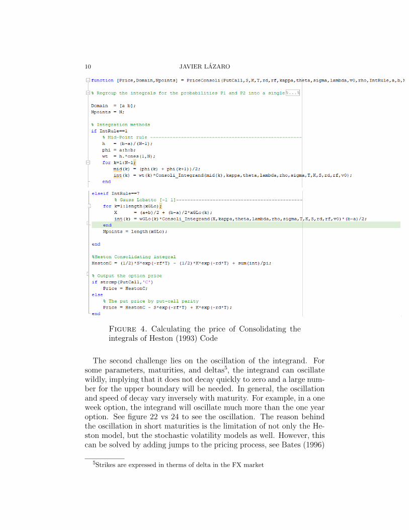
10 JAVIER LAZARO

Figure 4. Calculating the price of Consolidating theintegrals of Heston (1993) Code

The second challenge lies on the oscillation of the integrand. Forsome parameters, maturities, and deltas5, the integrand can oscillatewildly, implying that it does not decay quickly to zero and a large num-ber for the upper boundary will be needed. In general, the oscillationand speed of decay vary inversely with maturity. For example, in a oneweek option, the integrand will oscillate much more than the one yearoption. See figure 22 vs 24 to see the oscillation. The reason behindthe oscillation in short maturities is the limitation of not only the He-ston model, but the stochastic volatility models as well. However, thiscan be solved by adding jumps to the pricing process, see Bates (1996)

5Strikes are expressed in therms of delta in the FX market


[Bat96].

In order to solve the previous challenge, the right choice of b mustbe made. b can be chosen with the MD (multi-domain) integrationapproach of Zhu (2010) to select the upper limit. In this integrationapproach the domain [0,∞) will be represented by [a, b], where a shouldbe close to zero, and b is as big as desired. Once the integration intervalwhere the numerical method will be applied is defined, it is split intoN parts and each part is integrated as a whole. The probability is cal-culated as the sum of the area under the curve of each subinterval, butonly when the subinterval area is greater than a determined tolerancelevel. Otherwise, the subinterval area is not taken into account and thecalculation will stop.

As an example, one can consider the following case: an interval[a = 1e − 5, b = 150] used to represent [0,∞), N = 3 and a toler-ance level of 1e − 6 6. To implement the MD method, the interval isfirst split into N parts, [1e−5, 50], (50, 100], (100, 150]. The first inter-val is integrated by the decided method, and it yields a result greaterthan the tolerance level, meaning it will be summed up. The sameprocedure applies to the next intervals, and in this case, the result ofthe second interval is also greater than the tolerance. However, whenthe last interval is integrated, the resulting value is less than the tol-erance, and therefore it contributes little to the area. In other words,the integral decays to zero near 100, and therefore the last interval willnot be take into account. At this point the MD method will stop. Inthe example, the integration domain was reduced from [1e − 5, 150]to[1e− 5, 100] due to the MD. See figure5.

This method will assign a wider domain for shorter maturities anda narrower for longer ones. Zhu (2010) states that this is an optimalmethod for assigning the upper limit of the integral. However, if Nincreases, the computational time increases as well, due to the factthat instead of making one integral, it now has to make at least Nintegrals. Furthermore, the ad − hoc choice of the upper limit mustalways be done since the interval must be defined in all cases. Themost accurate way, regardless of the time, is to plot the integrates P1,2

for all the maturities and all the deltas, choose b based on the graph,and apply the MD method with a large N value. It is worth noting

6Using a small tolerance leven of ≤ 1e − 6 with M > 1e6 subintervals of areacoul lead to an error of order 1

12 JAVIER LAZARO

that other methods for finding b exist, such as the one in lewis (2000):b = max[1000, 10/

√v0τ ].

Figure 5. Multi Domain Function

The third challenge lies in the discontinuity of the CF over the do-main [0,∞). To solve this problem, the CF of Albrecher et al. (2007)was applied. Since ”The little Heston Trap” always works, other morecomplex alternatives to overcome this problem, like the rotation algo-rithm of Kahl and Jackel (2005) [KJ05] and the ones proposed on Zhu(2010) are not taken into account.See figure6.

The numerical methods taken into account were Newton-Cotes (here-after NC) rules and Gaussians Quadratures (hereafter GQ). Both ofthese approximate the remaining Heston integral over the domain [a, b]by equation (3.0.1). They calculate the area as the sum of the func-tion evaluated at the abscissas, x1, ...xN , multiplied by their respectiveweight w1, ...wN .


Figure 6. Multi Domain Function

(3.0.1)

∫ b

a

f(x) dx ≈N∑j=1

wj f(xj)

The NC rules are easy to understand since they are the simplest in-tegration rules. Unfortunately, they require the most computationaltime. Using equation (3.0.1) to defined the NC rules implies thatthe abscissas are equidistant, making the integration interval equalityspaced. This implies that computational time dramatically increasesfor an accurate integration because many abscissas are needed. Thedrawback of NC rules lies in calculating the weights since they are notequal for all the abcsissas and are method depending. The weights arealso dependent of N, the numbers of parts the intervals must be split in.

On the other hand, the GQ abscissas and weights, beside from beingless, are unequally spaced and calculated by functions depending onthe method. Each quadrature has one equation for the abscissas andone for the weight. The abscissas are specified in advance, so the up-per and lower boundary problem is solved. The disadvantage with this

14 JAVIER LAZARO

method lies on its complexity, however, once the abscissas and weightsare calculated, applying the method becomes a straightforward andtrivial exercise. The GQ substantially reduces the computational timevs NC due to the facts that the numerical method adapts to some howfit the integral. The value of the abscissas and weights depend on thechoice of N. In this study, N will be 32 for all GQ, following the guid-ance of Rouah (2014).

To numerically evaluate the Heston integrals P1,2 using the prosednumerical methods, the abscissas and weights must be calculated first.Then, as the following step, the integrand is evaluated at each abscissaand the result is multiplied by the corresponding weight. Once thisis done, the result is store in a vector and all the terms of the vectormust be added in order to calculate the integral. In other words, applyequation (3.0.1).

The numerical methods that were taken into account were: fourNC rules and three GQ. The following subsections introduce all thementioned numerical methods. The literature on numerical methods isrich and there are excellent text books like Burden and Faires (2010)[BF10] and Abramowitz and Stegun (1964), [AS64] which the readermay check for further details.

3.1. Mid-Point. It approximates the integral as the sum of rectangles,each with the same width, xj+1−xj, and height equal to the integrandevaluated at the mid point of the interval width. The Mid-point ruleis defined as:

(3.1.1)

∫ b

a

f(x) dx ≈ h

N−1∑j=1

f

(xj + xj+1

2

)where the abscissas are defined as xj = a+ (j− 1)h and the weights aswj = h = (b− a)/(N − 1),with x1 = a, xN = b.

The code used in this study to implement the Mid-Point numericalscheme 7 to calculate de Heston (1993) price is:

3.2. Trapezoidal Rule. It approximate the integral as the sum oftrapezoids, each with equal width, xj+1 − xj, and the height equalto the integrand evaluated at the end point of each subinterval. Thetrapezoids are constructed by drawing a segment between f(xj) andf(xj+1). The formula for the Trapezoidal rule is:


Figure 7. Mid-Point Code

(3.2.1)

∫ b

a

f(x) dx ≈ h

2f(x1) + h

N−1∑j=1

f(xj) +h

2f(xN)

where the abscissas and h are defined as the Mid-point rule. w1 =wN = h/2 and wj = h for j = 2, ..., N − 1.


Figure 8. Trapezoidal Rule Code

3.3. Simpson’s Rule. Each NC rule is more complicated than theprevious one and less than the subsequent. This NC uses quadraticpolynomials in the approximation, following Rouah (2014). The inte-gral is defined as:(3.3.1)∫ b

a

f(x) dx ≈ h

3f(x1) +

4h

3

N2−1∑

j=1

f(x2j) +2h

3

N2∑j=1

f(x2j−1) +h

3f(xN)

16 JAVIER LAZARO

where the abscissas and h are defined as the Mid-point and Trapezoidalrule, but with w1 = wN = h/3 along with wj = 4h/3 when j is even,and wj = 2h/3 when is odd.


Figure 9. Simpson’s Rule Code

3.4. Simpson’s 3/8 Rule. This rule is a refinement of the previousone. It uses cubic polynomials in the approximation of the integral andis the more sophisticated NC rule in this study. It is defined as:(3.4.1)∫ b

a

f(x) dx ≈ 3h

8f(x0)+

6h

8

N−3∑j=3,6,9,...

f(xj)+9h

8

N−1∑j 6=3,6,9,...

f(xj)+3h

8f(xN)

Note that this rule stars with x0 because the abscissas are defined as:xj = a + ih for i = 0, ..., N where N is divisible by three and withh = (b− a)/N . The weights depend on whether j is divisible or not bythree:

wj =

3h/8 if j = 0 or j = N6h/8 if j = 3, 6, 9, ...9h/8 if j 6= 3, 6, 9, ...

The implementation of all the NC rules presented here are straightfor-ward, although the calculation of the weights may be tricky at times.For the Simpson’s Rule and Simpson’s 3/8 rule one must be careful withthe fact that N must be divisible by three and that this will directlyaffect calculation of the weights.

The code used in this study to implement the Simpson’s Rule 3/8numerical scheme 10 to calculate de Heston (1993) price is:


Figure 10. Simpson’s Rule 3/8 Code

3.5. Gauss-Laguerre. This quadrature is specially relevant becauseit is designed for the domain [0,∞). Its abscissas are the roots of theLaguerre polynomial, LN(x), defined as:

(3.5.1) LN(x) =N∑k=0

(−1)k

k!

(N

k

)xk

where the last term in (3.5.1) is the binomial coefficient. The weightsfunction uses the derivative of LN(x) evaluated at each abscissas in thefollowing equation:

(3.5.2) wj =(n!)2exj

xj[L′N(xj)]2

The code used in this study to implement the Gauss-Laguerre nu-merical scheme 11 to calculate de Heston (1993) price is:

Figure 11. Gauss-Laguerre Code

3.6. Gauss-Legendre. This quadrature is designed for the domain[−1, 1] so in order to be used, one must modified the Heston domainthrough the transformation:

(3.6.1)

∫ b

a

f(x0) dx =b− a

2

∫ 1

−1

f

(b− a

2x+

a+ b

2

)dx

18 JAVIER LAZARO

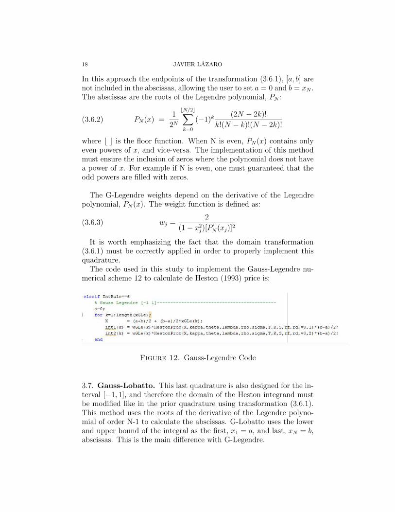
In this approach the endpoints of the transformation (3.6.1), [a, b] arenot included in the abscissas, allowing the user to set a = 0 and b = xN .The abscissas are the roots of the Legendre polynomial, PN :

(3.6.2) PN(x) =1

2N

bN/2c∑k=0

(−1)k(2N − 2k)!

k!(N − k)!(N − 2k)!

where b c is the floor function. When N is even, PN(x) contains onlyeven powers of x, and vice-versa. The implementation of this methodmust ensure the inclusion of zeros where the polynomial does not havea power of x. For example if N is even, one must guaranteed that theodd powers are filled with zeros.

The G-Legendre weights depend on the derivative of the Legendrepolynomial, PN(x). The weight function is defined as:

(3.6.3) wj =2

(1− x2j)[P

′N(xj)]2

It is worth emphasizing the fact that the domain transformation(3.6.1) must be correctly applied in order to properly implement thisquadrature.

The code used in this study to implement the Gauss-Legendre nu-merical scheme 12 to calculate de Heston (1993) price is:

Figure 12. Gauss-Legendre Code

3.7. Gauss-Lobatto. This last quadrature is also designed for the in-terval [−1, 1], and therefore the domain of the Heston integrand mustbe modified like in the prior quadrature using transformation (3.6.1).This method uses the roots of the derivative of the Legendre polyno-mial of order N-1 to calculate the abscissas. G-Lobatto uses the lowerand upper bound of the integral as the first, x1 = a, and last, xN = b,abscissas. This is the main difference with G-Legendre.


The weight function of G-Lobatto use the derivative of the Legendrepolynomials. The weight function is defined as:

(3.7.1) wj =2

N(N − 1)[PN−1(xj)]2

for j=2,...,N. However, for the end points the weights must be definedby the following expression:

(3.7.2) w1 = wN =2

N(N − 1)

To implement this method one can not set a = 0 because the first ab-scissa is x1 = a and the CF is not defined at zero.

All the mentioned approaches in chapter 2, Heston and the improve-ment ”Heston little trap” and consolidating the integral, were imple-mented with the seven numerical methods mentioned above, in orderto calculate the Heston price.

The Heston vector parameters, Θ = {κ, θ, σ, v0, ρ}, must be specifiedin order to completely describe and use the Heston model. The nexttwo chapter explain how Θ is found by two different methods: cali-bration by MSE and estimation by MLE. Those methods are twoconcepts that point to the same direction, one uses Q-measure in thesense of spot data, and the other P-measure in the sense of historicaldata.

The code used in this study to implement the Gauss-Lobatto numer-ical scheme 13 to calculate de Heston (1993) price is:

Figure 13. Gauss-Lobatto Code

4. OTC FX Option Market Convention

In general, OTC market options like the one in Colombia, quotethe option by delta rather than strike. This quotation method iscommon in OTC FX option markets, where buyers asks for a delta

20 JAVIER LAZARO

(i.e two months 25%∆Call) and the salesman or trader returns aprice (i.e 17, 358%) 7, as well as the strike (i.e 3200COP ), given thespot reference. This means that for a given maturity, spot, and rf , rd,the market has a k that must be found, in order to make the formula(4.0.1) equal to either 25% or 10%, depending on the case.

(4.0.1)

∆ = e−rf τN (d1)with

d1 =log(S/K)+(rd−rf+σ2/2)τ

σ√τ

The strikes can be found by a root-finding algorithm like Newton-Raphson or bisection, nevertheless, it can also be found analytically.Equation (4.0.2) presents the analytical solution to go from ∆ to k.

(4.0.2) K = S0 exp(−N−1(∆f )σ√τ + (rd − rf + σ2/2)τ)

were ∆f is the delta-forward. Given that the forward term has be-come relevant, the next two paragraphs will explain it.

There are four types of delta conventions used in the FX market,and the delta-forward is one of them.8 In equity markets, the delta,∆, gives the amount of underlying the seller of the option must buy tohedge. In FX markets, that type of delta is called delta-spot, ∆S, and itis equivalent to buying ∆S times foreign units of the option’s notional.The delta-forward, ∆f , is not only the derivative of the BSM optionprice with respect to the forward FX rate 9, ∂CBSM

∂f(t,T )= ∆f = N (d1),

but also the number of forward contracts that the seller of the optionneeds to delta-hedge. See Beier and Renner (2010) [BR10] for a com-plete description of the standard FX market conventions worth reading.

Usually, traders use forward contracts to hedge options, and sincethe market prices in delta forward convention, the option hedge canbe achieved much easier thanks to the quotations. For a better under-standing, an example will be given: a trader sells a COP-USD optionwith maturity in two weeks for a given spot reference with a ∆25 and acorresponding strike of 3200 COP. Once sold, the trader must hedge the

7The FX prices are often in terms of volatility or pips, not in currencies like COPor USD.

8Recall that delta, ∆ measures the rate of change of the price with respect tothe underlying, ∆ = ∂C/∂S where C stands for call price under BSM

9Express the BSM formula for FX market as C = erdτ [f(t, T )N (d1)−KN (d2)]

were d1 = ln (f(t,T )/k)+(σ2/2)τσ√τ

, d2 = d1 − σ√τ and f(t, T ) = Ste

rd−rf τ .


option. He needs to make the replicating portfolio or get in a forwardcontract with the same maturity and strike of the option. The chosenhedge is the forward contract, since the market already possesses theforward with the needed characteristic.

To summarize delta conventions, they express the strikes in termsof a BSM greek: delta can refer to spot or forward, amongst others,were spot means the delta hedge must be made in the spot market,and forward in the forward one. ATM convention will be presented inthe next paragraph.

The ATM-forward means that the strike is not equal to the spot,instead it is equal to the forward for the given maturity. This impliesthat by the put-call parity, Call−Put = erdτ (F (t, T )−K), this is thestrike at which the price of the call and put are the same. There is alsoa put call parity for deltas: ∆C −∆P = 1, that will be helpful since itmeans that 10∆ Put is equal to 90∆ Call and 25∆ Put to 75∆ Call.This is useful because in the Colombian OTC FX option market, themost traded deltas are 10∆ Put, 25∆ Put, ATM , 25∆ Call, 10∆ Calland they can all be expressed in terms of ∆C thanks to the put-callparity’s presented. For each delta, one can find 1W , 1M , 2M , 3M ,6M , 9M , and 1Y as maturities.

5. Estimation: Maximum Likelihood

This study uses the Atiya and Wall (2009) analytic approximationfor the likelihood function of the Heston model. Recall that the Hestonmodel does not define the volatility as a function of past asset obser-vations, instead, it defines it as a latent variable state in a stochasticprocess.

Because the underlaying distribution is not needed to price in theHeston model, it is not defined in the specifications, and therefore theclassical construction of the likelihood function can not be achieved.

Atiya and Wall (2009) suppose that the transition probability densityfor the joint log-underlying price/variance process from t to t + 1 isbivariate normal, were N denotes the normal density of meanµt+1 andcovariance matrix Σt+1. The following equation illustrates the supposedbivariate normal distribution:

22 JAVIER LAZARO

(5.0.1) p(St+1, vt+1|St, vt) = N (µµµt+1,ΣΣΣt+1)

To check the entire specifications of µµµt+1 and ΣΣΣt+1 see Atiya and Wall(2009).

Atiya and Wall (2009) defined the problem of estimating the volatil-ity as a ”filterinig problem” and formulated it as that of obtaining thelikelihood of the volatility given the past likelihood observations. Inother words, the variance likelihood must be approximated from theunderlying one. The likelihood at time t+ 1 is:

(5.0.2) Lt+1(vt+1) ∝ dt (abt)−1/4 e−2

√abtLt(vt)

the equation (5.0.2) is only approximate but it is valid because theapproximation error is small. This is due because the time step is short.That implies that the gap between the constand function and the con-tinues one are small. Please see Atiya and Wall (2009) for more details.

Once the likelihood is defined, calculating the log-likelihood is trivial.The above equation uses the following quantities:

(5.0.3)

a =(κ

′)2 + ρσκ

′dt+ σ2(dt)2/4

2σ2(1− ρ2)dt

bt =(vt+1 − αdt)2 − 2ρσ(vt+1 − αdt)(∆xt+1 − µdt) + σ2(∆xt+1 − µdt)2

2σ2(1− ρ2)dt

dt =1

Dexp

((2κ

′+ ρσdt)(vt+1 − αdt)− (2ρσκ

′+ σ2dt)(∆xt+1 − µdt)

2σ2(1− ρ2)dt

)with κ

′= 1 − κdt, α = κθ, D = 2πσ

√1− ρ2dt, initial values10

L0(v0) = e−v0 , the drift µ = rd− rf , and the log-underlying increments∆xt+1 = xt+1 − xt.

Atiya and Wall (2009) proposed a value for the time increment ofdt = 1/252 for daily data.

Note that bt, dt and also Lt+1(vt+1) depend on vt, and therefore, tocompute the likelihood, vt must be calculated first. Atiya and Wall(2009) notice that vt =

√bt/a and invert it in order to get:

10Here v0 is the initial variance parameter.


(5.0.4) vt+1 =√B2 − C −B

where

B = −αdt− ρσ(∆xt+1 − µdt),C = (αdt)2 + 2ρσαdt(∆xt+1 − µdt) + σ2(∆xt+1 − µdt)2 − 2v2

t aσ2(a− ρ62)dt.

To implement the estimation one must construct the likelihood usingthe following steps. First, calculate the quantities that do not change inthe likelihood construction such as α, a, D and the initial value L(v0).Second, calculate ∆xt+1 in order to find B and C, which are neededto obtain vt+1. Third, Atiya and Wall (2009) state, ”it is imperativeto combine the exponent in dt and the exponent −2

√abt before expo-

nentiating”. Doing this will avoid numerical errors. The reason is thatthere are some exponets that are large and almost of eaqual magnitudebut with opposite sign. Fourth, once dt and e−2

√abt are computed as

one, the remaining terms in (5.0.2) should be multiplied. Finally, afor-loop from step 2 until 4 for t = 0 to T − 1 must be made to obtainthe likelihood. Computing the log-likelhood is straightforward once theabove steps are understood.

The code used in this study to implement the Likelihood Atiya andWall (2009) estimation is 14.

It is worth mentioning that this study define v0 as a parameter anddo not uses a grid to define it.

The parameter found using the proposed data, initial values andMLE estimation method lead to: 15

6. Calibration: Non-Linear Least Square/ Mean SquareError

Calibration is a method, where a few parameters from the model aretweaked until they match with their counterpart market values, so thatthe model may fit with the market data. This is done by minimizingthe square distance between the model and market prices, which isknown as MSE. One can also minimize the model’s implied volatil-ity with the market one, as long as they both have the same dimensions.

This method calibrates the Heston vector parameter Θ = {κ, θ, σ, v0, ρ}by defining a function that minimize the square distance between the

24 JAVIER LAZARO

Figure 14. Likelihood AW Code


Figure 15. MLE Estimator

spot data and the model one. The minimizing parameters found arethe ones used. This implies that the market and the Heston prices areas similar as can be in square error. As explained before, the calibra-tion method finds the parameters under the risk-neutral measure, Q.

The function can be defined in one of two ways: as MSE or asIVMSE. The first, Mean Square Error or MSE, is defined as:

(6.0.1)1

N

∑t,k(∆)

wt,k(∆)(Cmktt,k(∆) − CH

t,k(∆))2

This function minimizes the square error between the market andHeston prices, where the subindex refers to all the possible combina-tions of the Colombian liquidity points: seven maturities and the fivestrikes (in terms of 10 and 25 deltas).

To apply the MSE function, one must retrieve the prices from themarket data which are in terms of delta-forward and an ATM-forward.The last two terms are quoted normally in OTC (over-the-counter) FXoption markets and they must be understood somehow in order to re-trieve the prices.

In brief, to apply the MSE function with the Colombian marketdata: deltas11 the market implied volatility expressed in combinationof 90∆ Call, 75∆ Call, ATM , 25∆ Call, 10∆ Call, and maturities1W , 1M , 2M , 3M , 6M , 9M , 1Y , must be used with equation (4.0.2)

11 The ∆Put were changed for ∆Call

26 JAVIER LAZARO

to find the respective strikes for the given deltas: MktIV–> Stike

followed by this apply BSM pricing formula to retrieve the pricesof the european vanilla call for all the combination of maturities anddeltas: Stike–> BSM Price. This means that one part of (6.0.1) isknow available to use : Cmkt

t,k(∆)

In addition,CHt,k(∆))

2 must be calculated so equation (4.0.2) can beused. For calibration purpuse this study calculate the Heston price byHeston (1993) with Gauss Laguerre.

The main disadvantage of the MSE is that short maturities, deepOTM with little value, do not contribute enough to the sum in (6.0.1).Hence, the optimization will tend to fits better ITM options with longermaturities. The weights used in this study for the MSE function areequal for all data. In order to solve the mentioned problem the enduser can change the weights by assigning a relative big weight to shortermaturities deep OTM.

The MSE function can also be defined with the implied volatilityof the market. The Implied Volatility Mean Square Error, IVMSE, isthe second way of defining the function.

(6.0.2)1

N

∑t,k(∆)

wt,k(∆)(IVmktt,k(∆) − IV H

t,k(∆))2

The IVMSE finds the parameter set, so that the implied volatilitiesof the model are as close as possible to those of the market. Implement-ing this function to calibrate the Heston model was done by followingthe following steps: express the deltas in terms of strikes for all matu-rities, compute the Heston prices with the given strikes and maturities,use a root-finding algorithm to find the BSM volatility that equal theHeston price with the market price, and finally, add up the square dif-ferences.

The main disadvantage of IVMSE is the need of a root-findingalgorithm which is numerically intensive. One remedy is to use theapproximation of the implied volatility that the Vol. of Vol. expan-sion series given by Lewis (2000), (A.3.4b). Another solution is toapproximate the IVMSE by the function given in Christoffersen etal. (2009). See [CHJ09]. The parameter set estimated from the lastmentioned method minimize the following function:


(6.0.3)1

N

∑t,k(∆)

(IV mktt,k(∆) − IV H

t,k(∆))2

V ega2t,k(∆)

were V ega2t,k(∆) = S0N (d1)

√τ is the BSM price equation sensitiv-

ity with respect to the implied volatility evaluated at the maturity andstrikes. This function offers a reduced computational time, however, itis done at the expense of a loss of accuracy. Christoffersen et al. (2009)states that the same function used to calculate the parameters mustbe used to evaluate the model fit.

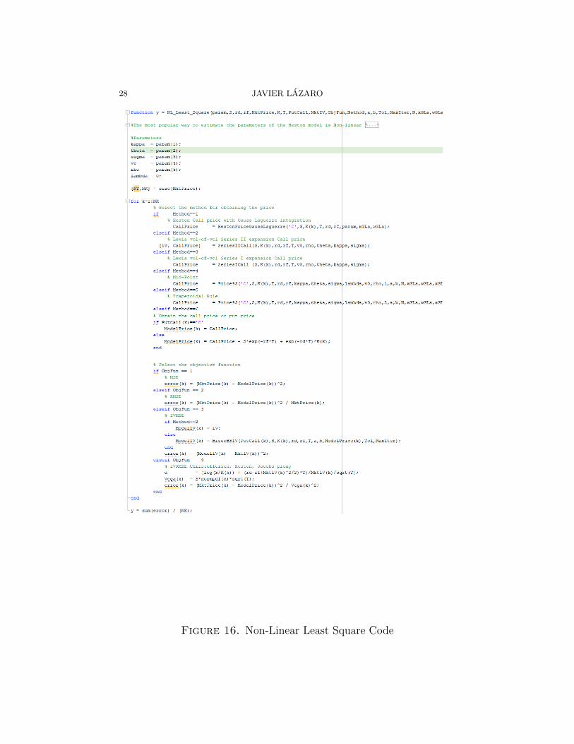
The code used in this study to implement the Non-Linear LeastSquare calibration 16 is:

There are considerable philosophical discrepancies between calibra-tion and estimation. Quants may argue that under the risk-neutraldistribution Q, the prices are arbitrage-free, but under P − measurethey are not. Econometricians may stand for a more robust method tofind the parameters set. They may argue that historical prices carry in-formation about the expected value of the price itself and therefore theparameters are arbitrage-free. Nevertheless, there is a similarity in ap-plying any of the methodologies, both algorithms may find the zeros inthe functions, maximize or minimize in order to find the parameter set.

7. An Accurate Implementation

This study calculates the Heston price with two equivalent pricingapproaches: (i) Heston (1993) and (ii) Consolidating the integrals

Because the optimization method used in this study depends on theStrike rather than Delta, one must find the Strike for the given Deltas.Furthermore, one can not assume there is a linear relationship betweenthe Delta and the Strike even though a one to one or injective functionmust exist between them. In other words, a delta can only have onestrike and viceversa, and that is a necessary and sufficient condition toproceed. The following graph shows the relationship.17

In order to implement the Heston model, the parameter set must bespecified first. This study uses the Matlab function fmincon to min-imize the NLLS and MLE. These optimization functions are stableand is highly accepted in different disciplines. The constraints used

28 JAVIER LAZARO

Figure 16. Non-Linear Least Square Code


Figure 17. Delta to Strike and Strike to Delta

are κ > 0, θ > 0, σ > 0, v0 > 0, ρ ∈ [−1, 1], starting valuesκ = 8, θ = 0.04, σ = 0.3, V0 = 0.05, ρ = 0.8 and some reason-able lower and upper boundaries. Moreover, due to the optimizationmethod used, one must define an upper boundary for all parameters.The code snippet illustrated in figure 18 shows the initial values, andthe lower and upper boundaries used in this study.

it is worth mentioning that σ and V0 are the volatility of volatilityand the initial value of the volatility of volatility.

It is worth mention that initial values were hardly found. The Colom-bian market requires a positive ρ and the goal was achieved by applyinga try and failure method in a neighborhood defined by the lower andupper bound.

30 JAVIER LAZARO

Figure 18. Initaial values, lower and upper bound

As with any optimization, it is important that the starting and truevalues do not lie too far from each other12. To achive that, one must becareful using empirical literature to define them because almost all ofthe reliable studies use index or stock data. For FX emerging marketsdata such as USD-COP, the ρ must be positive to ensure the mar-ket behavior: If the risk increases the investors will find shelter in thestrong pair leading to price increases. In other words, the literaturemay not be helpful in defining the starting values. In order to definethem one must focus on Fellers condition, 2κ∗θ > σ2, to ensure that σis allways positive. In the one week parameter set the condition is notmet due to the Stochastic model’s well known limitation. Zhu (2009)[Zhu09] calibrates V0 to the ATM implied volatility in the FX market,and suggest setting κ large enough so that Fellers condition is fulfilled.

In the FX literature the emerging market is not as popular as de-sired, because of the liquidity in the market. This implies that findinginitial values to used defining the parameter set is one of the papercontributions. The author remark in the dificult to find initial valuesthat lies to a positive correlation because parameter set was estimatefor each maturity. This implies that the values used are stable for theColombian FX market.

After the problem of the initial values parameter is solved, one canproceed to estimate the parameters used to find the Heston prices.This study estimates a set of parameters for each maturity due to therecomendation of [RH13]. The main difference in each estimation isthat the farther the maturity, the more data is used to estimate the setparameter. For example, in the estimation in the one week parameterset, only data from the previous week is considered, while for the onemonth parameter set, only data from the previous month is consid-ered, and so on. This is significantly important due to the fact that

12This is a Ansatz: Suppose this is true so that one can proceed.


Figure 19. Calibration snippets code

even though the same data may be used on multiple calculations, theamount of data used varies from calculation to calculation. The sameparameter accross every maturity must not lie too far form each other.The Matlab snippet of code used to calculate the parameters is shownin figure 19

The chosen non-linear least square function wasMSE because [RH13]suggests to use it. Once the parameters are found by the chosen methodone can proceed. It is worth mentioning that for the optimizationmethod to work, one must define a function to find the price of theHeston model. In other words, the optimization method uses a pre-selected Heston pricing equation, and the resulting parameters set willbe used to find the most accurate Heston price method. So the samevariable first will be endogenous and later it becomes exogenous. Thiscan be misleading, however, one may think that the pre-selected pric-ing method can be skewed, but that is never the case. No matter whatpre-selected pricing method the code uses, it is never the most accurate.

Once the estimation problem is overcome, one should find, in onehand, the more accurate method and, in the other, the computation-ally faster scheme, and combine both results to find the answer this

32 JAVIER LAZARO

Figure 20. MLE Vs. NLLE

study is looking for: a scheme that lasts the least amount of time pos-sible and a pricing method that shows as small an error as possible. Inorder to achieve this goal, a Ceteris Paribus analysis will take place,first finding the computationally Faster Scheme, and then the most ac-curate method.

In the next chapter the problem of the computationally faster schemwill take place.

8. Computationally Faster Scheme

In order to make the process of finding the computationally fastersolution, all the possible combinations of the pricing approach thatrequire to solve an integral with all the numerical schemes were com-puted one hundred times. In other words, the two integrals of Heston(1993) where calculated with the 7 numerical schemes. After the codecalculate the Heston (1993) price by 7 diferent ways, one must knowwhich of those 7 ways is the best. Understand the best as the scheme


that lasts the least amount of time possible and show the small error aspossible. Using the Ceteris Paribus analysis the problem become two:(i) the accurest method and (ii) the fastes one.

To solve the problem of the fastest numerical scheme one must mea-sure the time required to run the code. This study uses the Matlabfunction Timeit. This function calls the specified function multipletimes, and returns the median of the measurements to form a reason-ably robust time estimate. It also considers first-time costs. The Mat-lab function cputime was discarded because it could be misleading. Forfurther details on measure performance se http://www.mathworks.com/

This study uses more than one repetition to make more robust theanalysis because if the repetition are not enough, the conclusion of thestudy will be difficult to accept by the reader. To solve this problem,for each pricing method the code calculates an array of:

(repetition, Strike,Maturity, IntegrationScheme)

were: repetition=100, Strike=ATM, Maturity=[1W,2W,3W,1M,6M,9M,1Y],Integration Scheme=(i)Mid-Point (ii) Trapezoidal rule, (iii) Simpson’srule, (iv) Simpson’s 3/8 rule, (v) Gauss-Laguerre, (vi) Gauss-Legendreand (vii) Gauss-Lobato. In other word the array will have dimention:

(100, 1, 7, 7)

Figure 29 shows the array for a combination of a pricing aproach andscheme. There are 49 combinations of pricing methods and numericalschemes. For example:

(rep = 1, Strike = ATM,Maturit = 1W, IntegrationScheme = Mid−Point)

(rep = 2, Strike = ATM,Maturit = 1W, IntegrationScheme = Mid−Point)(rep = 3, Strike = ATM,Maturit = 1W, IntegrationScheme = Mid−Point)

.

.

.

(rep = 100, Strike = ATM,Maturit = 1W, IntegrationScheme = Mid−Point)

34 JAVIER LAZARO

is one combination, of Stike, Maturity and the integration schemeand the code sees it as a matrix. Particulary, all the 49 combinationthe code sees it as an array. The code uses nested loops to calculate allthe combination. ie. First make the 100 rep, of ATM strike and 1Wmarturity, then its go to 100 rep, ATM strike and 1M marturity. Afterthat its go to 100 rep of ATM strike and maturity of 2M, so on, untilthe maturity of 1Y. See Figure 29 and imagine the Array of:

(repetition, Strike,Maturit)

Now think that in that array lies data that use only mid-point nu-merical scheme to find those 700 price: 7 maturities, and 100 rep foreach

The study calculate the 29 array to all the numerical scheme. Thatmean that will be calculated 7 times. Imagine 30 as the form the codecalculate 100 rep, with the ATM strike, accross all the maturitis, andsolving the model integral with all the numerical shcheme this studyanalice. It is importand that the reader remeber that the integrandchange when the parameter of the model change. In this study theparametes change every time the maturity change due to the fack thatwe calculate a fiderent set of parameters to each maturity, and that liesin importand change in the integrand when the maturity change.

All of the above leads to an array dimension problem. To solve this,one must calculate the average smile time for each maturity and for allthe posible combinations of pricing methods and numerical schemes toget an array of dimention

(repetition = 100, Strike = 1,Maturity = 7, IntegrationScheme = 2) = (100, 1, 7, 2)

See Figure 21 and imagine the array.Once the code calcuates the mentioned array one can reduce the di-

mention to see the computationally faster scheme. Rember thar foreache calculation of price the code save the time it take to calculatethat price. The next challenge is to find another array that reflects the


Figure 21. Tiempo ATM

most accurate pricing method.

9. Accurate method

It may be assumed that the trapezoidal rule is the most accuratepricing approach since a curved line can be approximated by joiningstraight lines. For example, a circle can be defined as a polygon of infi-nite sides. Therefore, one can accurately calculate the Heston integralby applying the trapezoidal rule with the lower boundary as close aspossible to zero and an upper limit grater than the point where theintegral tends to zero. For the lower limit the study uses 1e-20000, anupper limit equal to 300 and divide that space in 10.000.000. The Fig-ure 22 , 23 ,24 and 25 show the integrals of Heston 1993 for maturityof 1 week and 1 year using MSE and NLLS

All the integrals were plotted to visually determine the point wherethe integral tends to zero, which resulted in the conclusion of using 300as the upper limit. This does not mean that the integrals in the Colom-bian market decay near that number. However, it can be ensured thatthe point of decay is less than the chosen upper limit.

In order to approximate a curved line that can be steep at the originbut highly oscillatory, the trapezoidal rule must divide the integrationinterval into a very large number of parts. This study divides the cho-sen integration domain [a, b] in 10 million parts. The drawback withthis implementation is the extremely high computational time it cantake to process this numerical method. The benchmark prices for allthe maturities and deltas have at least 41 decimal points, see figure 26,and take 1.5 hours to calculate each price.

Once the bechmark price has been determined, the MSE betweenthe benchmark and all the posible combinations of price methods and

36 JAVIER LAZARO

Figure 22. 1W Benchmark Integral using MLE parameters

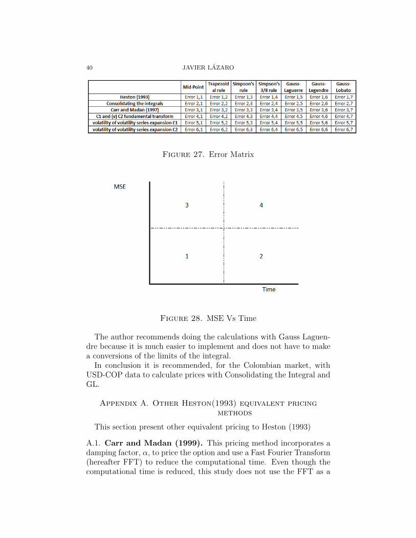
schemes must be calculated, in order to finally compute the average ofa given MSE price method across maturities. At the end one will havean MSE 7x7 matrix. See 27.

10. Joining the Average Time with the MSE

For each price method, a Time versus MSE plot is drawn after each ofthe axis variables are calculated. Based on these plots, one can proceedto a more detailed analysis by dividing each plot into four regions. Anexample of how this division should take place is shown in Figure 28.From the regions in the graph, the following conclusions can be derived:

• Region one is the goal behind this study, aiming at finding themost perfect balance between MSE and computational time foreach pricing method.• Region two and three vary in importance based on what the

code user is looking for. Where region two would appeal tothose who prefer to sacrifice more time in exchange for a more


Figure 23. 1W Benchmark Integral using NLLS parameters

accurate result, while region three would favor those with lesstime to spend.• Region four reflects the most undesirable ways to calculate the

Heston price.

In an ideal scenario, there would be six graphs, one for each pricingmethod. This would allow for the creation of a final graph displayingonly the top result from each pricing method. With this last graph,the best pricing method and numerical scheme would be selected.

It is worth mentioning that if any of the numerical calculations ofthe price, regardless of numerical schemes and price methods used, leadto a negative value, the price method will not be taken into account.The reason behind this lies in the fact that if a single price is nega-tive, there is a significant probability that other calculations using thesame method can yield more undesireable results. This does not implythat if all the results are possitive, other calculations using that samepricing method will not be negative, but the chances of calculating a

38 JAVIER LAZARO

Figure 24. 1Y Benchmark Integral using NLLS parameters

negative value are far lower. Since this study’s aim is based on numer-ical empirical evidence rather than a mathematical demostration, the4.901 results obtained from each pricing method are used to supportthe claims previously made in the paragraph.

11. Conclusions

All the pricing model where calculated at least 5 times, that impliesthat the study calculates . In all of them all the calculated pricesof Heston(1993) and consolidating the Heston integral were positive.That is a positive result due to the amount of time the price of thestochastic model was compute.

The model that least the last were consolidating the Heston integralbecause it does calculate one integral. In the other hand, the numericalmethod that have the smallest MSE is a draw between G-Legendreand G-Laguerre because its closeness is less than e-5. The remainingquadrature behaved the same way or with more error than conventionalmethods.


Figure 25. 1Y Benchmark Integral using NLLS parameters

Figure 26. Benchmark ATM Price using MLE andNLLS parameters

40 JAVIER LAZARO

Figure 27. Error Matrix

Figure 28. MSE Vs Time

The author recommends doing the calculations with Gauss Laguen-dre because it is much easier to implement and does not have to makea conversions of the limits of the integral.

In conclusion it is recommended, for the Colombian market, withUSD-COP data to calculate prices with Consolidating the Integral andGL.

Appendix A. Other Heston(1993) equivalent pricingmethods

This section present other equivalent pricing to Heston (1993)

A.1. Carr and Madan (1999). This pricing method incorporates adamping factor, α, to price the option and use a Fast Fourier Transform(hereafter FFT) to reduce the computational time. Even though thecomputational time is reduced, this study does not use the FFT as a



numerical scheme or option pricing method since the cost limitation isto high in the sense of loss of accuracy and handling. It entails a trade-off between the grid sizes, consequently, one can not willing chose theintegration grid. This restriction is due to the constrain λη = 2π

Nthat

entails the relationship between the integration grid and the log-strikegrid. Other approaches like the Fractional FFT applied by Chourdakis(2004) [Cho04] tries to solve the limitations of FFR by relaxing therestrictive constraint.

Carr and Madan (1999) uses a Fourier transform approach to op-tion pricing. The advantage of their method is the use of only oneintegral that decays faster than Heston (1993), in consequence thecomputational time is reduce. See Lord and Kahl (2007) [LK07] formore advantages of the approach. Carr-Madan shows that the ana-lytical solution to price a European call can be obtain once the CF isknown. This method notices that discounting the present value of thepayoff call, C(x), is not integrable L1, where x = ln k, and thereforethe following modified call price, c(x), is proposed:

42 JAVIER LAZARO

(A.1.1) c(x) = eαxC(x)

where eαx is the damping factor and is applied on C(x) to make thecall price integrable L1 and therefore the Fourier transform, c(x), forc(x) can be found.

(A.1.2) c(x) =e−rdτϕ(v − (α + 1)i)

α2 + α− v2 + iv(2α + 1)

where ϕ is f2(φ). To get the call price the inverse Fourier transformmust be used to recover c(x) and remove the damping factor to restorethe call price, C(x).

(A.1.3) C(x) =e−αx

π

∫ ∞0

Re[eivxc(v)

]dv

The main disadvantage of this approach is having to appropriatelychose the damping factor α since accuracy will be lost if the parameteris distant from the real one. This study uses Lee (2004a) [L+04] tofind a range of admissible values for α and implements the Lord andKahl (2007) method to find the optimal α∗. To implement Carr-Madanprice, one must replaced the spot price S by Se−rf τ , see Whaley (2006)[Wha06] for justification.

This study uses the following sniped code 32 to calculate the integral

A.2. Lewis (2000) Fundamental Transform. This approach re-

quires that the fundamental transform (hereafter FT), H(k, v, τ), andthe generalized Fourier transform of the option payoff, be available.Lewis 2000 [L+00] says: ”The FT is determined by the volatility pro-cess and not by the particulars of any option contract”, and definesthe FT as an analytic characteristic function with all its properties.This means that the FT is modeled without a contract dependencyand that the approach will only work with the Heston FT and not itsCF. Through Lewis’ book, some steps to follow for option pricing13 arepresented. Before these steps may be followed, one must obtain thegeneralized Fourier transform of the option payoff, which is easier toobtain than the option price itself, and the fundamental transform ofthe Heston model. It is worth mentioning that the fundamental trans-form of the Heston model is homologous to the CF.

13See page 39 of Lewis (2000) book


The generalized Fourier transform, unlike the regular Fourier trans-form, allows some arguments to be complex. The generalized Fouriertransform at maturity, f(k, T ) is call the payoff transform

(A.2.1) f(k, T ) = − Kik+1

k2 − ikwhere ki > 1 for a call option. The FT of the Heston model is not

straightforward, see Lewis (2000) for details of the derivation

(A.2.2)

H(k, v, τ) = exp(Ct +Dtv)

Ct = κθ

[κ+ d

2t− ln

(1− gedt

1− g

)]Dt =

κ+ d

2

(1− edt

1− gedt

)where κ = 2(κ+ikρσ)

σ2 , θ = κθκ+ikρσ

, d =√κ+ 4c, c = (k2−ik)

σ2 , g = κ+dκ−d .

Note that the FT, H(k, v, τ) (A.2.2) is equal to the Heston CF (2.1.6)with the notation Ct and Dt denoting Cj(τ, φ) and Dj(τ, φ). Oncethe payoff (A.2.1) and the FT (A.2.2) are known, the Lewis steps arestraightforward: (i) multiply the fundamental transform (A.2.2), thepayoff transform (A.2.1) and the expression exp([−rd − ik(rd − rf )]τ);(ii) pass the result trough the generalized inverse Fourier transform(A.2.3)

(A.2.3) f(x, t) =1

2π

∫ iki+∞

iki−∞eikxf(k, t) dk

where x = lnSt. (iii) evaluate the integral over the correct strips of

regularity, for which the FT, H(k, v, τ), and payoff, f(x, T ) would be:

(A.2.4)H(k, v, τ) :=

−κ+ d

2< ki <

−κ− d2

f(x, T ) := 1 < ki

Hence, the call price, C1(K), is:

(A.2.5) C1(K) = −Ke−rdτ

π

∫ ∞0

Re

[eikX

1

k2 − ikH(k, v, τ)

]dk

where X = ln(S/K) + (rd − rf ) and ki > 1.

44 JAVIER LAZARO

Lewis (2000) establishes another way to compute the call price basedon put-call parity and a covered call, for which the payoff ismin(ST , K).

The respective covered call payoff transform is f(k, T ) = Kik+1 / (k2−ik) and the FT is (A.2.2). Upon completion of the mentioned steps14

for the option pricing with the covered call, one can get:

(A.2.6)

C2(K) = Ste−rf τ − Ke−rdτ

π

∫ ∞0

Re

[eikX

1

k2 − ikH(k, v, τ)

]dk

Note that the values of C1 and C2 are the same, even though theexpressions are virtually identical, the different strips make the valueof the integrals distinct but operating with the remaining terms makesthe prices equal.

A.3. Lewis (2000) Volatility of Volatility Series Expansion.Pricing with the Heston model by the Vol. of Vol. expansion is compu-tationally faster because the approach does not solve an integral, likethe name says, the price is obtained by a series of sums. As a matter offact, the expansion derived its name from the powers of the volatility ofvolatility parameter, σ, from which the series are expressed in. Thereare two expansions, one for the price and one for the implied volatility,known as Series I and II respectively.

Series I is based on the BSM price

(A.3.1) CBS(S0, v T ) = S0e−rfTφ(d1)−Ke−rdTφ(d2)

where d1 = (log(S0/K) + (rd − rf + v2/2)T )/(√vT ) and d2 = d1 −√

vT . The expression, v, is the expected average variance over thelifetime of the option, (0, T ). It is defined as:

(A.3.2)

v = E

[1

T

∫ T

0

vt dt

∣∣∣∣ v0

]=

1

T

∫ T

0

E[vt|v0] dt

=1

T

∫ T

0

vt[θ + (v0 − θ)e−κT ] dt = (v0 − θ)(1− e−κT

κT) + θ

Series I also uses the BSM Vega evaluated at the expected aver-age variance, v. Note the importance of, v, in the derivation of thisapproach.

14The strip for step 3 is ki = 1/2


(A.3.3) Cv(S0, v, T ) =∂CBSM∂v

∣∣∣∣v=v

=

√T

8πvS0e

−rfT exp(−1

2d2

1)

As mentioned, the first series calculates the Heston price directly,meanwhile the second one provides the implied variance that serves asinput in the BSM pricing formula to compute the Heston price. SeriesI is (A.3.4a) while Series II is (A.3.4b).

(A.3.4a)

CI(S0, v0, T ) ≈ CBS(S0, v0, T ) + σJ1

TR1,1Cv(S0, v0, T ) +

σ Cv(S0, v0, T )

[J3R

2,0

T 2+J4R

1,2

T+

(J1)2R2,2

2T 2

](A.3.4b)CII(S0, v0, T ) = CBS(S0, vimp, T )

vimp ≈ v +J1R

1,1

T+

σ2

[J3R

2,0

T 2+J4R

1,2

T+

(J1)2

2T 2(R2,2 −R2,0(R1,1)2)

]Both series depend on the expected average variance, v, as well as

in the J1,3,4 and R equations. Lewis (2000) explains that J2 equationvanishes since the drift is linear. Each Js equation presented here isa solution of a respective integral with φ(1/2). The interested readermay check the integrals in Lewis 2000 for further details.

(A.3.5)

J1(v0, T ) =ρ

κ

[θT + (1− e−kT )(

v0

k− 2θ

k)− e−kT (v0 − θ)T

]J3(v0, T ) =

θ

2κ2

[T +

1

2κ(1− e−2κT )− 2

κ(1− e−kT )

]+

(v0 − θ)2κ2

[1

k(1− e−2kT )− 2Te−kT

]J4(v0, T ) =

ρ2θ

κ3

[T (1 + e−κT )− 2

κ(1− e−κT )

]− ρ2

2κ2T 2e−κT (v0 − θ) +

ρ2(v0 − θ)κ3

[1

κ(1− e−κT )− Te−κT

]

46 JAVIER LAZARO

Finally, the R equations are presented. They are BSM ratios usedto compute the Heston price.

(A.3.6)

R1,1 =

[1

2−W

], R1,2 =

[W 2 −W − 4− Z

4Z

]R2,0 = T

[W 2

2− 1

2Z− 1

8

]R2,2 = T

[W 4

2− W 3

2− 3X2

Z3+X(12 + Z)

8Z2+

48− Z2

32Z2

]where W = X/Z, X = log(S0/K) + (rd − rf )T, Z = vT .

Bibliography

[Ale08] C. Alexander, Market risk analysis, pricing, hedging and trading finan-cial instruments, Market Risk Analysis, Wiley, 2008.

[AMS] H Albrecher, P Mayer, and W Tistaert Schoutens, The little hestontrap, Wilmott Magazine, January issue, 83–92.

[AS64] Milton Abramowitz and Irene A Stegun, Handbook of mathematicalfunctions: with formulas, graphs, and mathematical tables, vol. 55,Courier Corporation, 1964.

[AW09] Amir F Atiya and Steve Wall, An analytic approximation of the likeli-hood function for the heston model volatility estimation problem, Quan-titative Finance 9 (2009), no. 3, 289–296.

[Bac05] K. Back, A course in derivative securities: Introduction to theory andcomputation, Springer Finance, Springer Berlin Heidelberg, 2005.

[Bat96] David S Bates, Jumps and stochastic volatility: Exchange rate processesimplicit in deutsche mark options, Review of financial studies 9 (1996),no. 1, 69–107.

[BF10] R.L. Burden and J.D. Faires, Numerical analysis, Cengage Learning,2010.

[BGZ11] Tim Bollerslev, Michael Gibson, and Hao Zhou, Dynamic estimation ofvolatility risk premia and investor risk aversion from option-implied andrealized volatilities, Journal of econometrics 160 (2011), no. 1, 235–245.

[BIB+15] E. Berlinger, F. Illes, M. Badics, A. Banai, G. Daroczi, B. Domotor,G. Gabler, D. Havran, P. Juhasz, I. Margitai, et al., Mastering r forquantitative finance, Community experience distilled, Packt Publishing,2015.

[Bjo09] T. Bjork, Arbitrage theory in continuous time, Oxford Finance Series,OUP Oxford, 2009.

[BM00] Gurdip Bakshi and Dilip Madan, Spanning and derivative-security val-uation, Journal of financial economics 55 (2000), no. 2, 205–238.

[BR10] Claus Christian Beier and Christoph Renner, Foreign exchange options:Delta-and at-the-money conventions, Encyclopedia of Quantitative Fi-nance (2010).


[BRSD10] Frederic Bossens, Gregory Rayee, Nikos S Skantzos, and Griselda Deel-stra, Vanna-volga methods applied to fx derivatives: from theory to mar-ket practice, International journal of theoretical and applied finance 13(2010), no. 08, 1293–1324.

[Cas10] A. Castagna, Fx options and smile risk, The Wiley Finance Series,Wiley, 2010.

[CHJ09] Peter Christoffersen, Steven Heston, and Kris Jacobs, The shape andterm structure of the index option smirk: Why multifactor stochasticvolatility models work so well, Management Science 55 (2009), no. 12,1914–1932.

[Cho04] Kyriakos Chourdakis, Option pricing using the fractional fft, Journal ofComputational Finance 8 (2004), no. 2, 1–18.

[Cla11] I.J. Clark, Foreign exchange option pricing: A practitioner’s guide, TheWiley Finance Series, Wiley, 2011.

[Coh15] G. Cohen, The bible of options strategies: The definitive guide for prac-tical trading strategies, Pearson Education, 2015.

[Con10] R. Cont, Encyclopedia of quantitative finance, 4 volume set, Wiley,2010.

[CS89] Marc Chesney and Louis Scott, Pricing european currency options: Acomparison of the modified black-scholes model and a random variancemodel, Journal of Financial and Quantitative Analysis 24 (1989), 267–284.

[FB73] Myron Scholes Fischer Black, The pricing of options and corporate lia-bilities, Journal of Political Economy 81 (1973), no. 3, 637–654.

[Gla04] P. Glasserman, Monte carlo methods in financial engineering, Appli-cations of mathematics : stochastic modelling and applied probability,Springer, 2004.

[GP51] J Gil-Pelaez, Note on the inversion theorem, Biometrika 38 (1951),no. 3-4, 481–482.

[GT11] J. Gatheral and N.N. Taleb, The volatility surface: A practitioner’sguide, Wiley Finance, Wiley, 2011.

[Haf04] R. Hafner, Stochastic implied volatility: A factor-based model, LectureNotes in Economics and Mathematical Systems, Springer Berlin Hei-delberg, 2004.

[Hes93] Steven L Heston, A closed-form solution for options with stochasticvolatility with applications to bond and currency options, Review offinancial studies 6 (1993), no. 2, 327–343.

[HKLW02] Patrick S Hagan, Deep Kumar, Andrew S Lesniewski, and Diana EWoodward, Managing smile risk, The Best of Wilmott (2002), 249.

[HN13] A. Hirsa and S.N. Neftci, An introduction to the mathematics of finan-cial derivatives, Elsevier Science, 2013.

[Hul12] J. Hull, Options, futures, and other derivatives, Options, Futures, andOther Derivatives, Prentice Hall, 2012.

[HW87] John Hull and Alan White, The pricing of options on assets with sto-chastic volatilities, The journal of finance 42 (1987), no. 2, 281–300.

[Iac11] S.M. Iacus, Option pricing and estimation of financial models with r,Wiley, 2011.

48 JAVIER LAZARO

[JYC09] M. Jeanblanc, M. Yor, and M. Chesney, Mathematical methods for fi-nancial markets, Springer Finance, Springer London, 2009.

[Kil06] Fiodar Kilin, Accelerating the calibration of stochastic volatility models.[KJ05] Christian Kahl and Peter Jackel, Not-so-complex logarithms in the he-

ston model, Wilmott magazine 19 (2005), no. 9, 94–103.[L+00] Alan L Lewis et al., Option valuation under stochastic volatility, Option

Valuation under Stochastic Volatility (2000).[L+04] Roger W Lee et al., Option pricing by transform methods: exten-

sions, unification and error control, Journal of Computational Finance7 (2004), no. 3, 51–86.

[LK07] Roger Lord and Christian Kahl, Optimal fourier inversion in semi-analytical option pricing.

[Lue98] David G. Luenberger, Investment science, Oxford University Press,1998.

[MCC98] Dilip B Madan, Peter P Carr, and Eric C Chang, The variance gammaprocess and option pricing, European finance review 2 (1998), no. 1,79–105.

[Nat94] S. Natenberg, Option volatility & pricing: Advanced trading strategiesand techniques: Advanced trading strategies and techniques, McGraw-Hill Education, 1994.

[Rei10] Dimitri Reiswich, The foreign exchange volatility surface, Ph.D. thesis,Frankfurt School of Finance & Management, 2010.

[RH13] F.D. Rouah and S.L. Heston, The heston model and its extensions inmatlab and c#, Wiley Finance, Wiley, 2013.

[RV12] F.D. Rouah and G. Vainberg, Option pricing models and volatility usingexcel-vba, Wiley Finance, Wiley, 2012.

[Sco87] Louis O. Scott, Option pricing when the variance changes randomly:Theory, estimation, and an application, Journal of Financial and Quan-titative Analysis 22 (1987), 419–438.

[Shr04] S.E. Shreve, Stochastic calculus for finance ii: Continuous-time models,Springer Finance Textbooks, no. v. 11, Springer, 2004.

[SS91] Elias M Stein and Jeremy C Stein, Stock price distributions with sto-chastic volatility: an analytic approach, Review of financial Studies 4(1991), no. 4, 727–752.

[Sto13] Santiago Stozitzky, General bounds for arithmetic asian option prices:Colombian fx option market application, Master’s thesis, The Universityof Edinburgh, 2013.

[SZ99] Rainer Schobel and Jianwei Zhu, Stochastic volatility with an ornstein–uhlenbeck process: an extension, European Finance Review 3 (1999),no. 1, 23–46.

[Web11] N. Webber, Implementing models of financial derivatives: Object ori-ented applications with vba, The Wiley Finance Series, Wiley, 2011.

[Wha06] Robert E Whaley, Derivatives: Markets, Valuation, and Risk Manage-ment 345 (2006).

[Wig87] James B Wiggins, Option values under stochastic volatility: Theory andempirical estimates, Journal of financial economics 19 (1987), no. 2,351–372.


[Wil06] P. Wilmott, Paul wilmott on quantitative finance, 3 volume set, PaulWilmott on Quantitative Finance, Wiley, 2006.

[Wil13] , Paul wilmott introduces quantitative finance, The Wiley Fi-nance Series, Wiley, 2013.

[Wys07] U. Wystup, Fx options and structured products, The Wiley FinanceSeries, Wiley, 2007.

[Zhu09] J. Zhu, Applications of fourier transform to smile modeling: Theory andimplementation, Springer Finance, Springer Berlin Heidelberg, 2009.

(Javier Lazaro) Cr 51a No127-49, Bogota, Colombia.E-mail address: [email protected]

50 JAVIER LAZARO


52 JAVIER LAZARO

Figure 32. Error Matrix

an accurate heston implementation with usd-cop data

Documents