an abstract of the thesis of matthew p. thompson for the
TRANSCRIPT


AN ABSTRACT OF THE THESIS OF
Matthew P. Thompson for the degree of Doctor of Philosophy in Forest Engineering
presented on March 19, 2009.
Title: Contemporary Forest Road Management with Economic and Environmental
Objectives
Abstract approved:
John Sessions
One of the basic questions facing transportation planners and road managers is
how to provide and maintain a road system that provides efficient access to the forest
while limiting adverse effects roads can have on water and soil resources. The purpose of
this study is to develop decision support models that will lead to improved economic and
environmental efficiency in the management of forest road networks. In particular, I
focus on developing techniques to facilitate tradeoff analysis and help landowners
identify optimal erosion control policies.
Forest roads contribute to accelerated erosion, which can degrade water quality
and aquatic habitat. Federal agencies in the Pacific Northwest are actively seeking to
remove and/or improve roads in order to restore watershed condition, and private

landowners face regulatory restrictions under the Clean Water Act and state forest
practice acts. Though the treatment that best achieves management objectives for a
single road can often be identified, at larger scales the combination of treatments to
assign to a suite of roads can become too large for enumeration. In these circumstances
decision aids can and have been used. This dissertation is comprised of five manuscripts
that pair industrial engineering and forest engineering principles in order to provide
relevant decision support tools to facilitate forest road management. The manuscripts
address a range of available treatments, including regular maintenance, upgrading, and
road removal.
The first chapter describes the challenges associated with erosion control, reviews
available road treatments, and summarizes salient applications of decision support for
road management, focusing on applications where controlling road-related erosion was
an objective. The second chapter introduces a tradeoff analysis framework for
controlling road-related erosion. The third chapter presents an algorithm for routing
maintenance vehicles (graders) across a forest road network in order to minimize total
tour length, a proxy for operating cost. Chapter four extends this work to a multi-
objective context, seeking efficient solutions that simultaneously minimize vehicle
operating cost plus grading cost and hazard weighted rut depth, a measure of
environmental performance. Chapter five develops optimal policies for recycling
aggregate from decommissioned forest roads, and demonstrates that recovery and reuse
of aggregate can subsidize road removal projects. Chapter six extends this work to a
multi-objective context, approximating the efficient frontier for length of road removed

and removal cost, and investigating further the potential for aggregate recycling to
effectively subsidize decommissioning projects. Chapter seven concludes the dissertation
with a review of the preceding chapters.

Contemporary Forest Road Management with Economic and Environmental
Objectives
by
Matthew P. Thompson
A THESIS
submitted to
Oregon State University
in partial fulfillment of
the requirements for the
degree of
Doctor of Philosophy
Presented March 19, 2009
Commencement June 2009

Doctor of Philosophy thesis of Matthew P. Thompson presented on March 19, 2009.
APPROVED:
Major Professor, representing Forest Engineering
Head of the Department of Forest Engineering, Resources, and Management
Dean of the Graduate School
I understand that my thesis will become part of the permanent collection of Oregon State
University libraries. My signature below authorizes release of my thesis to any reader
upon request.
Matthew P. Thompson, Author

ACKNOWLEDGEMENTS
This work was completed while the author was a recipient of the Wes and Nancy
Lematta and the Dorothy M. Hoener fellowships, for which he is very grateful. The
author expresses sincere appreciation for the patience, guidance and tutelage of John
Sessions. The author also expresses sincere gratitude to Kevin Boston and Arne Skaugset
for their instruction, advice, and collaboration. Much credit is due to David Tomberlin,
who initially attracted the author to this field of research, and who served as a committee
member from afar. Lastly, thanks to Claire Montgomery, who was an excellent teacher
and supervisor, and who graciously agreed to serve as the graduate representative.
Thanks also to my wonderfully supportive wife, Leslie, and to my family and
friends.

CONTRIBUTION OF AUTHORS
Dr. John Sessions was integral to all components of manuscript work, including
(but not limited to) identifying research objectives, recommending and synthesizing
relevant literature, facilitating analyses, helping with computational difficulties, and
editing written work. Dr. Sessions co-authored every manuscript, and was the lone co-
author on manuscripts relating to aggregate recycling (Chapters 5-6). Dr. Kevin Boston
co-authored manuscripts relating to the routing of maintenance vehicles (Chapters 3-4)
and application of technical efficiency for erosion control (Chapter 2). Dr. Boston helped
the author with data collection, develop of solution techniques, analysis of results, and
framing of issues. Dr. Arne Skaugset co-authored Chapter 2 in an editorial and advisory
capacity, and in general contributed to the author’s understanding of forest erosion
processes. Dr. David Tomberlin co-authored and provided field-collected road segment
data for Chapter 2, and introduced the author to computer-based decision support for
erosion control. Dr. Jeff Hamann co-authored Chapter 4, assisting with the literature
review, development of solution techniques, and simulation of forest and road data. Dr.
Hamann is not a member of the author’s graduate committee, but rather a recent graduate
of Oregon State University and former classmate of the author. Dr. Jeff Arthur, also not
a member of the graduate committee, co-authored Chapter 3 by providing support on
operations research methodologies. At the time this dissertation was submitted, Chapters
3 and 5 had been published, and Chapters 2, 4, and 6 were undergoing peer review.

TABLE OF CONTENTS
Page
1 Introduction……………………………………………………………………………..1
1.1 Statement of Objectives and Research Contributions………………………...1
1.2 Literature Review……….…………………………………….………………3
1.2.1 Forest Roads and Water Quality…………………………………….3
1.2.2 Forest Road Management………………………………………….10
1.2.3 Decision Support for Forest Road Management…………………...13
1.3 Technical Efficiency: A New Paradigm for Forest Road Erosion Control....18
1.4 Dissertation Outline………………………………………………………….23
1.5 References……………………………………………………………………29
2 Forest Road Erosion Control Using Technical Efficiency…………………………….36
2.1 Abstract………………………………………………………………………36
2.2 Introduction………………………………………………………………….36
2.3 Forest Road Erosion Control………………………………………………...41
2.4 Problem Formulation………………………………………………………...46
2.5 Solution Technique…………………………………………………………..47
2.6 Example Application………………………………………………………...50
2.7 Discussion……………………………………………………………………54
2.8 Conclusion…………………………………………………………………...56

TABLE OF CONTENTS (Continued)
Page
2.9 References…………………………………………………………………..58
3 Intelligent Deployment of Forest Road Graders..…………………………………….71
3.1 Abstract……………………………………………………………………..71
3.2 Introduction…………………………………………………………………71
3.2.1 Road Maintenance and Grading…………………………………..71
3.2.2 Grading Decisions………………………………………………....73
3.2.3 Grader Routing……………………………………………………74
3.2.4 Notation and Definitions……………………………………….…78
3.3 Tabu Search…………………………………………………………………79
3.3.1 Neighborhood Definition…………………………………………79
3.3.2 Tabu Search Implementation Details……………………………..81
3.3.3 Shortest Path Service Edge Insertion (SPSEI) Heuristic…………82
3.3.4 Tour Partition Heuristic…………………………………………..83
3.4 Computational Results……………………………………………………...84
3.5 Discussion…………………………………………………………………..88
3.6 Acknowledgements…………………………………………………………92
3.7 References…………………………………………………………………..93
4 Identifying Optimal Forest Road Grading Policies Using a Multi-Objective Evolutionary Algorithm………………………………………………………..121
4.1 Abstract…………………………………………………………………….121

TABLE OF CONTENTS (Continued)
Page
4.2 Introduction………………………………………………………………..122
4.3 Problem Statement…………………………………………………………129
4.4 Solution Method……………………………………………………………135
4.5 Algorithm Design…………………………………………………………..138
4.6 Example Applications………………………………………………………141
4.7 Discussion…………………………………………………………………..149
4.8 Conclusion………………………………………………………………….152
4.9 References…………………………………………………………………..155
5 Optimal Policies for Aggregate Recycling from Decommissioned Forest Roads……174
5.1 Abstract……………..………………………………………………………174
5.2 Introduction…………………………………………………………………175
5.3 Aggregate Recovery and Reuse…………………………………………….180
5.4 Applications of Aggregate Recycling………………………………………183
5.5 Optimal Aggregate Management Policies………………………………….186
5.6 Example Application……………………………………………………….191
5.7 Results………………………………………………………………………194
5.8 Discussion…………………………………………………………………..197
5.9 Conclusion………………………………………………………………….201
5.10 Acknowledgements……………………………………………………….202

TABLE OF CONTENTS (Continued)
Page
5.11 References…………………………………………………………………204
6 Exploring Environmental and Economic Tradeoffs Associated with Aggregate Recycling from Decommissioned Forest Roads………………………………..216
6.1 Abstract……………………………………………………………………..216
6.2 Introduction………………………………………………………………...217
6.3 Formulating Optimal Aggregate Recycling and Road Removal Policies….222
6.4 Example Application……………………………………………………….228
6.5 Results……………………………………………………………………...233
6.6 Concluding Remarks……………………………………………………….236
6.7 References………………………………………………………………….240
7 Conclusion……………………………………………………………………………257
7.1 Forest Road Erosion Control Using Technical Efficiency (Chapter 2)…….262
7.2 Intelligent Deployment of Forest Road Graders (Chapter 3)……………….263
7.3 Identifying Optimal Forest Road Grading Policies Using a Multi-Objective Evolutionary Algorithm (Chapter 4)……………….....266
7.4 Optimal Policies for Recycling Aggregate Recovered from Decommissioned Forest Roads (Chapter 5)……………………………269
7.5 Exploring Environmental and Economic Tradeoffs Associated with
Aggregate Recycling from Decommissioned Forest Roads (Chapter 6)……………………………………………………………..270

TABLE OF CONTENTS (Continued)
Page
7.6 References………………………………………………………………….274
8 Bibliography………………………………………………………………………….275

LIST OF FIGURES
Figure Page
2.1 Efficient Frontier, 3 Segment Example…………………………………………….63
2.2 Modified Epsilon-Constraint Algorithm…………………………………………...64
2.3 Efficient Frontier, 47 Segment Example…………………………………………...65
3.1 Example network to illustrate allowable “swaps”………………………………….95
3.2 Current Solution: [A, B] → [C, D]………………………………………………...96
3.3 1-edge swap: [B, A] → [C, D]……………………………………………………...97
3.4 2-edge swap: [C, D] → [A, B]……………………………………………………...98
3.5 2-edge swap: [D, C] → [A, B]……………………………………………………...99
3.6 Network 1………………………………………………………………………….100
3.7 Network 2………………………………………………………………………….101
3.8 Network 3………………………………………………………………………….102
3.9 Network 4………………………………………………………………………….103
4.1 Road network for Example #1…………………………………………………….159
4.2 Non-Dominated Frontier, Mutation Rates = 1% and 80%, Example #1………….160
4.3 Non-Dominated Frontier (NDF) vs. Simulated Policy Solutions, Example #1…..161
4.4 Non-Dominated Frontier (NDF) vs. Simulated Policy Solutions, Example #1…..162
4.5 Road network for Example #2…………………………………………………….163
4.6 Non-Dominated Frontier (NDF) vs. Simulated Policy Solutions, Example #2…...164
5.1 Road Plan for the South Zone, with project types labeled…………………………207
LIST OF FIGURES (Continued)
Figure Page
6.1 Road plan for the South Zone of the McDonald Dunn Research Forest, with project types labeled……………………………………………………..244
6.2Knowledge base used to evaluate the potential aquatic environmental impact
of each road segment slated for decommissioning…………………………….245 6.3Comparison of non-dominated frontiers identified using various
decommissioning costs ($/km), with aggregate recycling permitted…………246 6.4Comparison of non-dominated frontiers, solved with and without the opportunity
to recycle aggregate from decommissioned roads…………………………….247 6.5Comparison of non-dominated frontiers, solved with and without the opportunity
to recycle aggregate from decommissioned roads…………………………….248 6.6Effective subsidy (ES), as it varies with environmental performance levels………249 6.7Influence of the recovery factor on non-dominated frontiers, calculated assuming a
decommissioning cost (DC) of $20,000/km…………………………………..250

LIST OF TABLES
Table Page
2.1 Example Inventory of Sediment Reduction and Treatment Cost……………………66
2.2 Road Segment Information, Case Study…………………………………………….67
3.1 Example deadhead and grading times, for the example network presented in figures 1-5……………………………………………………………………104
3.2: Possible candidate solutions from swaps, for the example network presented in Figures 1-5……………………………………………………………………...105
3.3 Computational results for Network 1………………………………………………106
3.4 Computational results for Network 2………………………………………………107
3.5 Computational results for Network 3………………………………………………108
3.6 Computational results for Network 4………………………………………………109
3.7 Results for Oregon State Research Forest network………………………………...110
4.1 Loaded Log Truck Traffic Regimes, Arranged by Timber Sale, Example #1……..165 4.2 Total Traffic (Light Vehicle, Rock Haul, Log Truck) over all Road Segments,
Example #1…………………………………………………………………….166 4.3 Segment-level grading frequency for each simulated management policy,
Example #1……………………………………………………………………..167 4.4 Size of the space covered (S) and coverage of two sets (C) for various mutation
rates, Example #1……………………………………………………………….168
4.5 Loaded Log Truck Traffic Regimes, Arranged by Timber Sale, Example #2……..169
4.6 Size of the space covered (S) and coverage of two sets (C) for various mutation rates, Example #2……………………………………………………………….170
5.1 Unit costs ($ / m3) for aggregate from decommissioned roads, local borrow pit,
and quarry; WADNR example………………………………………………….208

LIST OF TABLES (Continued)
Table Page
5.2 Total aggregate costs, with and without aggregate recycling, for scheduled maintenance and construction projects in the road plan for the WADNR Highway Alder Timber Sale……………………………………………………209
5.3 Aggregate demanded (Djt) for maintenance and construction projects (m3),
by period for the South Zone example………………………………………….210 5.4 Removal costs (hikt) and aggregate available (Ait) from spurs slated for removal
(m3); South Zone example……………………………………………………...211 5.5 Unit costs ($ / m3) for aggregate procured from decommissioned roads and
quarry; South Zone example……………………………………………………212 5.6 Unit Costs ($/m3) for procurement, processing and delivery (gsjt) of aggregate
from sources (abandoned roads and quarry) to other road segments in need of aggregate…………………………………………………………………….213
5.7 Cost savings and additional kilometers of road decommissioned over the
baseline, cost-minimization scenario; South Zone example……………………214 5.8 Results for the environmental benefit maximization model; South Zone
Example...............................................................................................................215 6.1 Aggregate demanded (Djt) for maintenance and construction projects (m3),
by period for the South Zone example………………………………………….252 6.2 Removal costs (hikt) and aggregate available (Ait) from spurs slated for removal
(m3); South Zone example……………………………………………………...253 6.3 Unit Costs ($/m3) for procurement, processing and delivery (gsjt) of aggregate
from sources (abandoned roads and quarry) to other road segments in need of aggregate……………………………………………………………………254
6.4 Road segment information passed into knowledge base to evaluate each road
segment’s relative effect on the aquatic environment……………………….....255 6.5 Calculated truth values scores representing the degree of truth of the assertion, “the
road has a high potential for causing damage to the aquatic environment.”…..256
LIST OF APPENDICES
Appendix Page
3.1 Listing of randomly generated service edges for Networks 1-4………………….111 3.2 Input segment-level data for Artificial Network 1………………………………..112 3.3 Input segment-level data for Artificial Network 2………………………………..113 3.4 Input segment-level data for Artificial Network 3………………………………..114 3.5 Input segment-level data for Artificial Network 4………………………………..115 3.6 Input segment-level data for the Oregon State Research Forest Network………..117 4.1 Listing of input segment-level input data for Example #2, Oregon State Research
Forest planning example………………………………………………………171

1 Introduction
1.1 Statement of Objectives and Research Contributions
One of the basic questions facing transportation planners and road managers is
how to provide and maintain a road system that provides efficient access to the forest
while limiting adverse effects roads can have on water and soil resources. The purpose of
this study is to develop decision support models that will lead to improved economic and
environmental efficiency in the management of forest road networks. In particular, I
focus on developing techniques to facilitate tradeoff analysis and help landowners
identify optimal erosion control policies.
Weaver and Hagans (1999, p. 236) present a five-step process for forest road
erosion prevention and control:
1. Problem identification (through inventory and assessment)
2. Problem quantification (determination of future yield in the absence of treatment)
3. Prescription development (both heavy equipment and labor-intensive)
4. Cost-effectiveness evaluation and prioritization of treatment sites
5. Implementation
This dissertation targets step #4, cost-effective evaluation and prioritization of
treatment sites. The intent is to develop computer-based decision support methods that
better integrate environmental objectives into forest transportation planning. I consider
planning contexts involving the scheduling of regular maintenance (grading), upgrading,

2 and removal. To model environmental performance I consider a range of possibilities,
including an assumed benefit from grading, as well as rut depth, sediment
production/delivery, and hazard weighted length of roads decommissioned.
As is relevant here, I consider a decision aid to be the paring of appropriate
mathematical formulations with solution methods. I employ both exact and heuristic
solution methods, depending upon problem size and complexity. For single objective
problems, I use traditional mixed integer programming as well as the tabu search
metaheuristic. For multiple objective formulations, I employ the epsilon-constraining
algorithm paired with mixed-integer programming, as well as multi-objective
evolutionary algorithms (MOEA).
This dissertation reflects an interdisciplinary approach, integrating forest
engineering principles with a diverse array of other fields, including applied economics,
combinatorial optimization, multi-objective optimization, multi-criteria decision making,
graph and network theory, computer science, and evolutionary computation. My research
contributions include:
• The novel application of the concept of technical efficiency to forest road erosion
control
• The identification of techniques to improve the environmental and economic
efficiency of forest road management
• The extension of decision support frameworks from single to multiple objective
formulations
3
• The illustration of the role of tradeoff analysis in informing forest road planning,
in particular improving understanding of marginal cost/benefit relationships
• The development of vehicle routing algorithms to intelligently deploy forest road
maintenance vehicles
• The development of optimal aggregate recycling and road removal policies
• The advancement of the notion that aggregate recycling can effectively subsidize
road decommissioning projects
1.2 Literature Review
1.2.1 Forest Roads and Water Quality
Forest roads benefit the landowner by providing access for timber production,
research, fire management, recreation, and other activities. However, forest roads are not
entirely benign and can lead to negative ecosystem impacts. In particular, forest roads
contribute significantly to degradation of water quality and aquatic habitat. They are
associated with accelerated erosion and can be a major source of sediment delivery to
streams (Jones et al. 2000; Lugo and Gucinski 2000; Forman and Alexander 1998).
Elevated levels of in-stream sediment can negatively affect salmonids through mortality,
reduced growth rates, disruption of egg and larvae development, and reduction in
available food (Newcombe and MacDonald 1991; Hicks et al. 1991). Poorly located or
designed stream-crossing culverts on forest roads create barriers to fish passage, which
can reduce salmon productivity (Nehlsen et al. 1991). Degradation of aquatic habitat is

4 of special concern in the western United States where endangered salmonid species
spawn and rear in watersheds containing potentially erosive forest roads. Maintenance of
high quality, unobstructed habitat is crucial to successful conservation efforts (GAO
2001).
The presence of a forest road can substantially and adversely alter natural
hillslope hydrologic and geomorphic processes. Forest roads intercept rainfall and
subsurface flow, concentrate flow on the surface or adjacent ditches, and divert or reroute
water from natural flow paths (Gucinski et al. 2001). They also accelerate chronic and
episodic erosion processes, alter channel structure and geometry, alter surface flowpaths,
and cause interactions of water, sediment and woody debris at engineered stream
crossings (Gucinski et al. 2001). Chronic erosion contributes fine sediment and is
generated by surface erosion processes along the road prism (Reid and Dunne, 1984).
Episodic erosion occurs in the form of mass-wasting and fluvial erosion due to culvert
failures and is often triggered by intense rain events (Reid and Dunne, 1984).
In areas with steep slopes, landslides and other mass movements are responsible
for the majority of episodic road-related erosion (Furniss et al. 1991). Chronic inputs
from road surface erosion can also be a significant source of sediment related input to
streams (Gucinski et al. 2001; Reid and Dunne 1984). Timber hauling during the wet
season can be the most significant source of fine sediment associated with forest practices
(Oregon Department of Forestry 2003). Fine sediment can originate from the road
surface itself due to the breakdown of the aggregate over time from crushing under heavy
tire loading and weathering. Sediment production is related to many road design

5 elements, including segment length and gradient (Luce and Black 1999), aggregate
quality (Foltz and Truebe 2003), and aggregate depth (Skaugset et al. 1997).
Management activities such as maintenance and especially log truck traffic also influence
sediment production (Luce and Black 2001; Bilby et al. 1989; Reid and Dunne 1984).
Road drainage systems are designed to move water away from the road surface as
quickly as possible, ideally to the forest floor where the water can disperse and infiltrate
into the soil. A critical factor affecting surface drainage is the road’s surface shape, i.e.
the cross-section of the travelling surface. Surface shapes are designed to “encourage
shedding of water from the surface before it gains enough concentration and velocity to
cause unacceptable surface erosion” (Moll et al. 1997, p.1). Unfortunately, in some
circumstances poorly designed and/or maintained drainage systems deposit sediment
directly into streams at road-stream crossings.
Improperly designed and/or maintained roads can contribute disproportionately to
aquatic habitat impairment. Often forest roads are built with limited effort to control
compaction, resulting in variable subgrade strength across road segments (Boston et al.
2008). Those areas with weak subgrades are more susceptible to localized surface
failures, such as potholes, washboards (lateral channels), and ruts (longitudinal channels).
A rut occurs where the vehicle load exceeds the bearing strength of the surface or
subsurface. Rut depth varies with tire operating pressure and traffic levels (Foltz and
Elliott 1998), as well as local conditions such as road material and moisture. Excessive
rut depth jeopardizes the road structure and can interfere with normal function of the
road’s designed drainage system. Concentration of water in the wheel rut increases

6 runoff length and water velocity, with the potential to detach and transport additional
particles. Sediment production from roads with ruts has been shown to be nearly double
that of roads without ruts (Burroughs and King 1989).
Road management issues vary by location and ownership. On federal lands in the
Pacific Northwest, the Aquatic Conservation Strategy (ACS) targets forest roads for
improvement and removal as an integral component of strategic watershed restoration
(Reeves et al. 2006). The aim of watershed restoration is to restore habitat and prevent
further degradation across landscapes (Heller 2002), and generally entails restoring
isolated habitats and improving or decommissioning roads, among other treatments (Roni
et al. 2002). The ACS cites preventing road-related runoff and sediment production as
two important components of its watershed restoration program (Reeves et al. 2006;
USDA and USDI 1994). Monitoring of ACS implementation indicates that the most
improved watersheds had relatively extensive road removal programs (Gallo et al. 2005).
These road removal programs generally focused on removing roads from riparian areas
and areas with high landslide hazard (Reeves et al. 2006).
The emphasis on removing forest roads in the ACS is, in part, a reflection of the
poor state of many of the transportation networks on federally owned lands. Though the
USDA Forest Service’s Road Management Policy (USDA 2001) states the goal of
reversing adverse ecological impacts associated with roads, the unfortunate reality is that
most roads in the national forest system are chronically under-maintained, with a backlog
of necessary improvement and removal needs (Sample et al. 2007; USDA 2002). As of
2002, less than 20% of the roads in the national forest system were maintained to the

7 desired standard (USDA 2001). A report by the Pinchot Institute for Conservation
recommended that national forests analyze their road systems to identify surplus roads
that can be decommissioned (Sample et al. 2007).
Though the ACS emphasizes road removal as a restoration activity, it is important
to note that removing roads does not in all circumstances ensure net environmental
benefit. Removing an excessive amount of roads could restrict access for fuel reduction
activities and fire control. Removing roads also limits future opportunities for biomass
recovery for alternative energy generation. Where lands are to be managed for timber
production, reducing road density would lead to increased skid trail length, which can
degrade soil resources, and could lead to increased utilization of helicopter logging,
which significantly increases fuel consumption. Decision makers therefore face tradeoffs
when selecting road segments for removal.
On private and state owned lands, where timber production remains more of a
dominant management objective, attention is focused less on removing legacy roads and
more on minimizing risk while maintaining an economically efficient transportation
network. In Oregon, the road systems on state and private lands appear in better shape
than the federal lands. A 1998 inventory of forest road drainage systems in western
Oregon revealed that 25% of the 285 miles of forest road surveyed delivered sediment
directly to streams (Oregon Department of Forestry 1998). Since then, industrial
ownerships in Oregon have gone to great lengths to improve their road networks (Chris
Jarmer, Director, Water Policy and Forest Regulation, Oregon Forest Industries Council,
personal communication, 2009). This improvement reflects funding and a deliberate

8 effort to upgrade road systems, whereas federal land management agencies have faced
decreased funding. Nevertheless, opportunities for additional improvement remain.
Beyond general stewardship obligations, the Clean Water Act (CWA) provides a
strong motivation to pursue effective erosion control methodologies on state and private
lands. Road-related sediment is recognized as a contributing source of pollution for
many rivers and streams listed as water quality limited under the CWA (e.g.,
Environmental Protection Agency, Impaired Waters and Total Maximum Daily Loads:
Examples of Approved Sediment TMDLs,
http://www.epa.gov/owow/tmdl/examples/sediment.html). Dai et al. (2004), for instance,
identified forest roads as the dominant source of controllable erosion in a decision aid
designed to support monitoring and assessment for a sediment total maximum daily load
(TMDL) in a northern California watershed.
In 1999, the EPA published proposed changes to the TMDL rules that would
significantly strengthen the nation’s ability to achieve clean water goals by ensuring that
the public had more and better information about the health of their watersheds (EPA
1999). The result has been increased interest in sediment production from forest roads.
Though the CWA in some circumstances allows for a balancing of economic interests
and promotes a progressive approach to pollution control premised on technological
innovation over time, it remains a national goal to attain “fishable and swimmable” water
quality (CWA §101(a)(2)).
Further, contemporary court precedent relating to the CWA suggests that
additional regulations concerning forest practices, especially forest road management,

9 may be forthcoming. A Federal District Court in California recently found that drainage
ditches and culverts delivering sediment to streams constitute point sources of pollution,
thereby subjecting forest roads to National Pollutant Discharge Elimination System
(NPDES) permitting requirements (EPIC v. PALCO, No. C 01-2821 MHP). However, a
different outcome was reached on a similar case in Oregon, with the Court ruling
effectively that all road-related sediment delivery is more accurately characterized as
nonpoint source pollution (NEDC v. Brown, No. 06-1270-K1). NEDC v. Brown was
appealed in the US Court of Appeals for the 9th Circuit. If a ruling by the appellate
Court aligns with the EPIC decision, it could usher in a new regulatory paradigm,
presenting new challenges to landowners seeking to cost-effectively control erosion.
NPDES permits require polluters to adhere to effluent limitation standards.
Technology-based standards reward efficiency and innovation, and tighten over time as
the state of the art evolves. Standards vary with the nature of the pollutant, but all are
premised upon the application of pollution control technology. As sediment is
considered a “conventional” pollutant, Best Conventional Pollution Control Technology
(BCT) standards would likely apply. As is relevant here, BCT standards “include
consideration of the reasonableness of the relationship between the costs of attaining a
reduction in effluents and the effluent reduction benefits derived.” (CWA §304(b)(4)(B))
This test for what constitutes “reasonable” is frequently referred to as the “bend of the
knee” test, where polluters are required to reduce pollution up to the point where the
marginal benefits per dollar spent begin to markedly decline. That is, the CWA presents

10 a statutory requirement to perform a cost/benefit tradeoff analysis in order to establish
pollution control standards.
Improving the environmental performance of forest roads therefore remains
important to both public and private landowners. Public managers must retain
transportation networks sufficient for timber production, fire prevention, public
recreation, and other access needs, while at the same time improving and
decommissioning roads in accordance with the Aquatic Conservation Strategy. Private
managers likewise must ensure their transportation networks meet timber production and
other access needs, while complying with state and federal regulatory constraints
designed to protect water quality. Contemporary forest road management thus involves
identification of a suite of road treatments that best achieve conflicting economic and
environmental criteria.
1.2.2 Forest Road Management
Appropriate road management can mitigate the environmental impact of the road
system by limiting chronic erosion and reducing the risk of large-scale episodic events
(Weaver and Hagans 1999). Management treatments to control road-related erosion
include regular maintenance, improvement (upgrading), and removal (closure or
decommissioning). Regular road maintenance can limit some of the deleterious effects
associated with rough road surfaces (i.e., roads with ruts and/or washboards). Grading is
the most common form of maintenance, wherein a bladed vehicle smoothes and re-shapes
the road surface. For industrial-sized ownerships grading can be a part of day-to-day

11 operations, and in some circumstances roads may be graded, or serviced, several times in
a month. By eliminating ruts and other failures, grading may simultaneously be able to
reduce both the environmental impacts and vehicle operating costs. Too frequent grading
can unnecessarily increase grading costs, and may in some cases actually lead to
environmental degradation by loosening the road surface and making available fine
sediment for delivery to streams (Luce and Black 1999). However, compacting,
watering, and/or applying chemical additives to the road surface after grading can help
reduce sediment production. Too infrequent grading, on the other hand, increases
transportation costs and the risk of environmental degradation associated with ruts. The
transportation planner therefore faces tradeoffs between economic and environmental
objectives when identifying grading maintenance regimes.
Beyond maintenance, there exists a range of available road restoration treatments,
from simple upgrading to full decommissioning (USDA and USDA 1994). Upgrading a
road may involve removing soil from sites with high landslide risk, installing additional
cross-drain culverts, modifying drainage systems to reduce connectivity with the stream
network, applying rock to the road surface, changing the road template, and
reconstructing stream crossings. Upgrading a road may reduce the rate of surface erosion
and likelihood of future road failure, but the road will remain open.
Roads no longer required for transportation can be closed and/or
decommissioned. High maintenance needs or high levels of environmental damage are
also reasons to decommission a road. Closing a road frequently consists of barricading or
gating the road to prevent unauthorized use, particularly during wet seasons, outsloping

12 the surface and installing rolling dips and/or waterbars, and may involve removing some
high-risk culverts. A closed road can be re-opened for future use or later
decommissioned, and generally requires only periodic inspection. Decommissioning a
road may involve removing culverts under significant fills, ripping the roadbed,
recontouring hillslopes, and may include planting or seeding the road surface. A
decommissioned road is not passable and requires no future maintenance. A common
goal of decommissioning is to restore the natural hydrologic processes and prevent future
sedimentation; a decommissioned road has lower longer-term environmental impacts
than a closed road due to significantly reduced risk of chronic and episodic erosion
(Switalski et al. 2004; Kolka et al. 2004; Madej 2001; Trombulak et al. 2000; Weaver and
Hagans 1999; Harr and Nichols 1993).
Road decommissioning decisions are complex and influenced by a variety of
factors, such as road location, sediment delivery risk, and available resources. Often only
a few “problem” roads produce the majority of the sediment, and it therefore may be
efficient to direct efforts towards those roads first (Luce and Black 1999). Weaver and
Hagans (1999) contend that it is rarely cost-effective to undertake a decommission
project without first evaluating its relative importance to overall watershed condition.
Similarly, Luce et al. (2001) state that road removal efforts must be prioritized, and argue
that management criteria should include economic and social concerns. Lugo and
Gucinski (2000) agree that decommissioning decisions should not be made based upon
ecological criteria alone, and caution that in some cases the environmental disruption
from decommissioning may be less desirable than leaving the road to reach some level of

13 stability. Anderson et al. (2006) point out that decommissioning decisions involve
weighing the relative risks of road failure, limited access for fire suppression, and limited
access for future market opportunities.
During decommissioning, it is often possible to recover aggregate from the road
surface. Recovered aggregate can be delivered to other roads for concurrent maintenance
or construction projects, with associated recovery and delivery costs. Alternatively,
aggregate required for maintenance or construction can be obtained from either local pits
or quarries with associated procurement and delivery costs. Re-use of the recovered
aggregate within the forest road network may significantly reduce rock transport distance,
especially when quarries are far away. Previous experience (Sessions et al. 2006; Mark
Truebe, Assistant Forest Engineer, Willamette National Forest, personal communication,
2007; Jennie Cornell, Washington State Department of Natural Resources, personal
communication, 2007) suggests opportunities for significant cost savings, even for small-
scale projects. These cost savings can effectively subsidize decommissioning projects,
suggesting an economic benefit associated with improving environmental benefit. A
major thread of this dissertation is the investigation of the potential for aggregate
recycling to lead to improved environmental performance, in addition to the investigation
of appropriate decision support tools for road maintenance, upgrading and removal.
1.2.3 Decision Support for Forest Road Management
Controlling road-related erosion to minimize sediment delivery and degradation
of aquatic habitat remains an important issue for forest stewardship. Managers are faced

14 with the task to develop efficient road management strategies to achieve conflicting
ecological and economic goals. Identification of an appropriate suite of road
management treatments can be difficult. Blanket prescription of best management
practices can prove ineffective and economically infeasible (Barrett and Conroy 2002); in
general it is not an efficient approach to apply treatments to problem areas independently
of their impact on overall cost-effectiveness (Weaver and Hagans 1999).
Though it may be possible on a segment by segment basis to identify the optimal
treatment, when the decision space extends over broad temporal and spatial scales for
entire road networks the pool of possible treatment combinations becomes too large for
explicit consideration (Anderson et al. 2006). That is, it is no longer sufficient to
evaluate treatment alternatives independently of one another. O’Hanley and Tomberlin
(2005), for instance, demonstrate how a simple heuristic to select fish passage barriers for
removal according to cost/benefit ratios alone can lead to inefficient and undesirable
resource allocations. What is required is some mechanism to facilitate generation and
evaluation of alternatives. In these decision-making environments, decision aids can and
have been used to facilitate decision-making.
To prioritize treatments, and to assess how well environmental objectives are met
as a result of treatment, environmental performance measures for forest roads are
required (Mills 2006). Common metrics include estimates of sediment production and/or
delivery (e.g., Rackley and Chung 2008; Brooks et al. 2006; Bettinger et al. 1998), road
roughness (e.g., Thompson et al. 2007; Provencher 1995), rut depth (e.g., Faiz and
Staffini 1979), and length of roads treated (Madej et al. 2006). Another approach is to

15 assign segments a hazard-weight based upon a set of criteria and attributes. Use of a
hazard factor enables differentiation between road segments based upon salient
characteristics such as proximity to a stream, erosive potential, etc. Similar approaches
include Thompson and Sessions (2008), who maximized the hazard-weighted length of
roads decommissioned, and Girvetz and Shilling (2003), who assigned environmental
impact scores to negatively weight roads for a least cost network path analysis. Boston
and Bord (2005) suggest manipulative experiments to improve our understanding
between forest road construction practices, material properties, and environmental
performance.
A prerequisite for prescribing road treatments is the generation of predictive, or
“forward looking,” sediment inventories. Absent estimates of treatment efficacy, it is
impossible to prioritize alternative treatments on the basis of cost/benefit. Allison et al.
(2004, p. 184) state, “the systematic consideration of each road section together with its
alternative restoration treatments reflects an appropriate diligence in generating a ranking
of restoration choices.” The California North Coast Regional Water Quality Board has
codified this best management practice into their General Waste Discharge Requirement
program, requiring forestland owners to develop and implement Erosion Control Plans to
“prevent and minimize the discharge of sediment” prior to initiating timber harvest
(Robert Klamt, North Coast Regional Water Quality Control Board, personal
communication, 2007). Erosion Control Plans must contain an inventory identifying
potential discharge sources, their locations, and estimated sediment volume, as well a
description and timeline of prevention and minimization measures that will be used.

16
Despite the apparent presence of conflicting objectives, most applications of
decision support for forest road management have considered a decision-making
environment with a single objective. A common approach assumes the decision-maker
manages to minimize treatment costs or maximize profits, absent environmental
considerations. Olsson (2007) compared deterministic and stochastic programming
techniques to determine optimal road upgrade treatments. Anderson et al. (2006) used
dynamic programming to determine optimal road class and deactivation strategies.
Karlsson et al. (2006) paired a mixed integer linear programming model with GIS-based
maps to facilitate road upgrading decisions in order to avoid losses associated with
blocked roads. Olsson and Lohmander (2005) used mixed-integer formulations to
optimize roundwood transport and road investments.
In some applications, environmental benefit as a result of road treatment is
implicitly modeled in cost minimization frameworks. Thompson et al. (2007) used a tabu
search heuristic to identify low cost tours for a maintenance vehicle to take, implicitly
assuming a benefit from grading. Thompson and Tomberlin (2005) similarly assumed an
environmental benefit associated with erosion control. They applied stochastic dynamic
programming to minimize the cost of erosion control on an unused logging road in the
Caspar Creek watershed in northern California (also see Tomberlin et al. 2002), where
the decisions included whether to maintain, upgrade, or decommission the road. Rackley
and Chung (2008) used NETWORK 2000 (Chung and Sessions 2003) to design road
networks with minimal haul and construction costs, incorporating erosion concerns by
assigning extra costs to road segments based upon expected erosion.

17
Transportation planning formulations that explicitly include environmental
concerns often model environmental objectives as constraints under an economic
objective. Contreras and Chung (2006) used an ant colony heuristic algorithm to identify
the set of least cost routes from timber sales to mills, with sediment production
constraints. Similarly, Bettinger et al. (1998) used tabu search to schedule harvest and
road activities with sediment production constraints to achieve aquatic habitat goals.
Akay and Sessions (2005) created a forest road alignment model that used a heuristic
procedure to minimize construction, maintenance and construction costs for forest roads,
while considering sediment production; this work has been further advanced by Aruga et
al. (2007).
Alternatively, the decision-maker can seek to optimize an environmental
objective, subject to budgetary constraints and other resource limitations. Thompson and
Sessions (2008) presented a mixed integer programming framework for determining
optimal levels of aggregate recycling and assigning road removal treatments, using
hazard-weighted length of roads decommissioned as an environmental proxy. Madej et
al. (2006) and Eschenbach et al. (2005) applied dynamic programming and genetic
algorithms to maximize the sediment saved from entering the stream channel as a result
of applying various treatments to roads and stream crossings. Allison et al. (2004)
applied a decision analysis framework to generate a ranking of the expected benefits of
proposed deactivation strategies for forest roads in steep terrain, where benefits were
expressed in terms of avoided damages from road-related slope failures.

18
As an alternative to modeling objectives as constraints, multiple objectives can be
condensed into a single objective function using methods such as goal programming or
weighting objectives. Goal programming requires identification of target environmental
performance levels. Both techniques require an appropriate mechanism to scale non-
commensurate objectives (e.g., $ and kg sediment), as well as a priori elicitation of
preferences between objectives. In such cases, multi-criteria decision models (MCDM),
which provide for the systematic elicitation of preferences between objectives, can be of
use (de Steiguer et al. 2003). Coulter et al. (2006), for example, used the Analytic
Hierarchy Process to condense three objectives (minimize impacts to streams, minimize
road failures, and minimize Forest Practice Act violations), then solved for the resultant
single objective function using a combinatorial heuristic.
1.3 Technical Efficiency: A New Paradigm for Forest Road Erosion Control
Arguably the aforementioned decision support approaches are unsuitable for road
erosion control under conflicting economic and environmental objectives. Kennedy et al.
(2008) referred to the notion of identifying a singularly “optimal” solution to such
problems as a “fallacy of the weighted sum approach,” because preferences can change,
and because no single answer simultaneously optimizes all objectives. Further,
identification of appropriate goals for sediment reduction (or some other metric) is not a
trivial task. As with other environmental management contexts, such as managing for
wildlife habitat objectives, a priori establishment of target values is a difficult, uncertain
exercise. Contreras and Chung (2006) set as an upper bound the estimated sediment

19 delivery associated with the minimal cost solution found absent sediment constraints,
then arbitrarily reduced that amount by 17%. Bettinger et al. (1998), to the contrary,
established sediment production goals from estimates of impacts from the previous 10
years of harvest activity within the study watershed. Notably, the authors acknowledged
the inherent difficulty and ambiguity in establishing such a goal. Rackley and Chung
(2008) avoided the difficulties associated with identifying target sediment production
levels by instead assigning a dollar value to sediment, but noted the challenge of selecting
an appropriate environmental cost factor.
This dissertation instead assumes that the decision-maker explicitly wants to
understand the tradeoffs prior to rendering an opinion on how to allocate weights
between objectives, on how to scale non-commensurate objectives, or on what
environmental targets/goals should be. More specifically, the decision-maker wants to
understand the relationship between increasing road treatment costs and increasing
environmental performance, and in so doing identify a tradeoff curve comprised of
“technically efficient” solutions1. A solution is considered efficient when it is impossible
to improve one objective (e.g., reduce cost.) without degrading another objective (e.g.,
increase sediment delivery). Efficient solutions are also referred to as “non-dominated”
or “non-inferior.” In this context, a multi-objective approach to optimization is required.
Employing multi-objective formulations is appropriate for environmental decision-
1 In the multi-objective optimization literature, the term “Pareto optimality” is often used to refer to what is defined by economists as technical efficiency, which is a necessary but not sufficient condition for Pareto optimality. Pareto optimality is defined as the allocation of wealth or resources between individuals such that no reallocation can make one individual better without making another individual worse off (Pearce 1992). The multi-objective optimization literature abstracts from notions of individual welfare and utility curves, considering instead objective functions to be optimized.

20 making, can lead to informed compromise, and should ultimately facilitate tradeoff
analysis (Kennedy et al. 2008; Toth et al. 2006).
A general multi-objective problem (MOP) can be formulated as shown below
(Jozefowiez et al. 2008):
⎩⎨⎧
∈=
=Dxts
xfxfxfxF n
..))(...,),(),(()(min
MOP)( 21 (1)
where n ≥ 2 is the number of objective functions, F(x) the objective vector, D the feasible
solution space, and x = (x1 ,x2, …, xr) the vector of decision variables. Consider two
decision vectors ., Dba ∈ Using the concept of technical efficiency, a is said to
dominate b )( ba p iff:
{ } { } )()(:...,,2,1)()(:...,,2,1 bfafnjbfafni jjii <∈∃∩≤∈∀ (2)
The set of efficient solutions is known as the efficient frontier or non-dominated
frontier, whose values represent tradeoffs in the objective space. Identifying these
solutions facilitates the decision maker’s selection of a compromise solution that satisfies
the objectives as best as possible (Van Veldhuizen and Lamont 2000). This represents an
a posteriori optimization approach, wherein the decision-maker selects a solution from
the frontier. By contrast, the a priori optimization approaches described earlier require
that preferences, which can be uncertain and change over time, be identified as inputs to
the optimization process.
Where multiple efficient alternatives exist, as is commonly the case, a secondary
layer of decision making is necessary in order to select from the set of efficient, or non-
dominated, solutions. Kangas and Kangas (2005) identify this as effectively the last step

21 in forest planning, wherein the “best” alternative is identified from among those
alternatives deemed efficient with respect to management objectives. Again, MCDM can
be used in such situations to elicit preferences, in order to help decision-maker(s) choose
from among competing solutions (de Steiguer et al. 2003). MCDM are also helpful in
situations where decisions are made by more than one individual, and where there exist
multiple stakeholders with differing opinions on how forest management should proceed.
Mendoza and Martins (2006) offer an excellent review of previous applications of
MCDM, as well as offering insight into new directions for modeling approaches moving
forward. The focus in this dissertation is developing techniques to identify the efficient
frontier, not to select an alternative from the frontier.
To date in the forest transportation planning literature there are few examples of
multi-objective approaches that consider environmental performance. Thompson and
Sessions (2008) employed exact methods to schedule road management treatments in
order to minimize treatment cost and maximize environmental benefit, but only solved
for the boundary solutions (i.e., they did not generate the tradeoff surface). Stückelberger
et al. (2006) presented a road network design framework with three objectives: minimize
road construction and maintenance costs, minimize deleterious ecological effects, and
maximize suitability of cable-yarding landings. They approximated the non-dominated
frontier with simulated annealing using an iterative approach, varying weights for a
scaled single-objective function. Unfortunately this method is only guaranteed to find all
efficient solutions if the frontier is convex. The presence of binary variables assigning
particular treatments to particular road segments means in most transportation planning

22 contexts the frontiers will not be convex. Manuscripts presented in this dissertation
therefore employ more appropriate multi-objective programming approaches. A notable
multi-objective paper that does not explicitly address road-related environmental
concerns uses the tabu search heuristic to identify the efficient frontier between lost forest
productivity and road construction costs (Richards and Gunn 2000).
To reiterate, transportation managers face a tradeoff between economic and
environmental objectives. In some cases the environmental objective is institutional, as
with federal agencies and the Aquatic Conservation Strategy, and in others the objective
may be imposed, as with private landowners subject to regulations concerning water
quality. The challenge therefore becomes to manage in order to achieve a low-cost,
environmentally-benign road network.
Identifying the efficient frontier provides valuable information on what is and is
not possible with respect to efficient management, and can point out instances where
current management practices are inefficient. The efficient frontier also provides
valuable information regarding tradeoffs in the objective space. In some circumstances a
landowner may opt for marginal increases in expenditure in order to significantly
improve the environmental performance of their road network. In others, a landowner
may be able to demonstrate that costs associated with additional protective measures are
not justified given the marginal benefit. Barrett and Conroy (2002), for instance, relate
an experience with the Pacific Lumber Company (PALCO) wherein a systematic analysis
of road treatment alternatives resulted in the identification of a road management strategy
that was both less expensive and perceived to be more effective at reducing

23 sedimentation than mitigation measures that were imposed as part of a habitat
conservation plan.
Employing techniques presented here allows for the identification of the set of
possible efficient outcomes, giving the decision-maker more insight into the problem and
helping to reach a suitable compromise solution (Toth et al. 2006). Public managers
facing reduced road maintenance budgets (due in part to reduced timber sales on national
forests) should be able to use methods demonstrated here to improve their treatment
efficacy. In particular, approaching aggregate recycling as an effective way to subsidize
road removal efforts should result in more roads being removed and ultimately contribute
to achieving strategic watershed restoration objectives. Private landowners should also
embrace the paradigm shift proposed in this dissertation, in order to evaluate their current
practices, identify where improvements can be made, and possibly to demonstrate that
additional regulatory restrictions are unnecessary or impractical.
1.4 Dissertation Outline
The subsequent chapters of this dissertation are comprised of five manuscripts
relating to various aspects of forest road management, plus a concluding chapter
summarizing results. Chapter 2 introduces the notion of using technical efficiency for
erosion control, in a scenario where various treatments to upgrade or remove a road can
be employed. I use the WEPP:Road sediment prediction model (Elliot et al. 1999) to
provide estimates of sediment delivery for each road segment, for each possible
treatment. First a very small hypothetical example is constructed to illustrate how

24 identification the set of non-dominated solutions may inform road treatment
prioritization. Next I apply the model to a larger network using field-collected road data
from the Jackson State Demonstrate Forest in northern California (Ish and Tomberlin
2005). I employ the epsilon-constraint method (Haimes et al. 1971), which iteratively
solves for one objective subject to increasing constraint levels representing the other
objective, in order to approximate the efficient frontier. Because of the small network
sizes I am able to use exact methods (GAMS v 22.7, CPLEX solver) to identify
intermediate solutions within the epsilon-constraint algorithm.
Chapters 3-4 instead focus on routing road maintenance vehicles (i.e., a grader)
over a road network. In Chapter 3 I model grader routing as the Rural Postman Problem
(RPP), the intent of which is to determine a minimal cost closed walk of a subset of some
arcs of a graph (Eiselt et al. 1995). The RPP formulation provides a basis for many other
industrial applications, including street sweeping, school bus routing, snow plowing, and
garbage collection (Corberán et al. 2000, Eiselt et al. 1995). I formulate a single
objective model to minimize total operating time, a proxy for grading cost. Reducing
grading cost could release resources for other maintenance needs, ideally resulting in a
better-maintained road system. Prior to deploying the grader, a subset of road segments
requiring grading is identified using a rubric based on road standard and roughness index.
A combinatorial optimization method, tabu search, is combined with two local search
procedures to generate efficient grading routes. Initially I examine the heuristic’s
performance on a variety of small cyclical and dendritic networks that vary with respect
to graph density, the optimal solutions to which can be found. Then I consider a much

25 larger road network, using a portion of the road network from the McDonald Dunn
Forest, a research forest managed by the College of Forestry at Oregon State University.
In Chapter 4 I extend the work of Chapter 3 to simultaneously consider economic
and environmental objectives, and to schedule routes over a planning horizon involving
multiple periods. This chapter approaches grader scheduling decisions as a multi-
objective vehicle routing problem, using a multi-objective evolutionary algorithm
(MOEA) as the solution method. The specific algorithm is known as SPEA2, (Strength
Pareto Evolutionary Algorithm 2), which maintains an external archive (i.e., secondary
population) of non-dominated solutions, and has been demonstrated to perform well in
comparative analyses (Zitzler et al. 2001). The economic objectives sums grader
operating cost and vehicle operating costs, and the environmental objective sums the
hazard weighted rut depth over all segments in the network. Hazard weights are assigned
to each segment according to the ratio of segment length over total network length. The
importance of segment length is emphasized based upon research by Foltz and Elliott
(1998) citing flow path length as an important variable. An empirical model developed
by the World Bank (Faiz and Staffini 1979) is used to model both vehicle operating costs
and rut depth formulation as a function of cumulative traffic. This problem is similar to
solving a sequence of postman problems (as in Chapter 3), but differs in that there is no
pre-identified subset of edges that actually require service, and that the costs are dynamic.
Portions of the McDonald-Dunn Forest’s road network are again modeled for purposes of
experimentation.

26
Chapters 5-6 focus on identifying optimal aggregate recycling policies, and
corresponding optimal road removal policies. The chapter presents real-world examples
of aggregate recycling and discusses the advantages of doing so. Further, the chapter
presents mixed integer formulations to determine optimal levels of aggregate recycling
under economic and environmental objectives. The objectives are thought to be
representative of management policies common among public managers in the western
United States. Here benefit is modeled as the hazard weighted length of roads
decommissioned. Two road removal treatments are considered: closure and
decommissioning, with the expectation that decommissioning entails significantly greater
environmental benefits. It is assumed an experienced professional has identified which
road segments require removal, and that the decision variable is whether to close or
decommission a particular road segment. If a road is decommissioned, the aggregate can
be recovered and used for other scheduled maintenance and construction projects. Again,
a portion of the McDonald-Dunn Forest’s road network is used for purposes of
experimentation (as is the case with Chapter 6). Comparing optimization results with and
without the opportunity to recycle provides quantitative information on the degree to
which aggregate recovery and reuse may simultaneously provide economic and
environmental benefits. Sensitivity analysis is performed with respect to
decommissioning cost and aggregate recovery rates.
Chapter 6 extends the work of Chapter 5 to simultaneously consider economic
and environmental objectives. That is, I seek to identify the entire frontier of efficient
solutions, not just the boundary (minimal cost, maximal benefit) solutions identified in

27 Chapter 5. The epsilon-constraint method is again employed. Chapter 6 also extends the
analysis of the role of aggregate recycling in effectively subsidizing removal projects. I
define an accounting variable ES (effective subsidy) as the difference in minimized cost
between scenarios with and without the opportunity to recycle aggregate, at a given level
of environmental performance. I then examine how ES varies with increasing levels of
environmental performance. The expectation is that ES generally increases with
increasing environmental performance, because as more roads are decommissioned more
low-cost aggregate may become available.
Chapter 6 also extends the work of Chapter 5 to include explicit calculation of a
hazard factor. In Chapter 5, the model assumes that all road segments slated for removal
are equally detrimental, and therefore the optimal treatment from an environmental
perspective is simply a function of length. This assumption is reasonable if it is also
assumed an experienced professional has identified appropriate levels of
decommissioning such that the expected future impacts per unit length from each
segment are nearly identical. With Chapter 6 to the contrary each segment is assigned a
score on the scale (0, 1) reflecting the degree to which the segment has potential to cause
environmental damage. Scores are assigned according to a model based upon the
Ecosystem Management Decision Support (EMDS) system. EMDS employs fuzzy logic
and knowledge-based reasoning integrated into a geographic information system (GIS) to
provide decision support for ecological assessment (Reynolds 1999). EMDS assesses
ecological condition according to a hierarchical, multi-criteria framework. The use of
fuzzy, or approximate, logic is thought to extend the ability to reason with the imprecise

28 or qualitative information common to natural resource management (Reynolds et al.
2000). EMDS has been employed for a variety of purposes, including characterization of
ecological condition and prioritization of watersheds for restoration on public land in the
Pacific Northwest (Reeves et al. 2006), watershed assessment in the Chewaucan Basin
(Reynolds and Peets 2001), assessment of habitat and basin-wide health in the Rogue
River drainage (Pess et al. 2003), sediment total maximum daily load monitoring in a
northern California watershed (Dai et al. 2004), and landscape evaluation of the eastern
Washington Cascades (Reynolds and Hessburg 2005). Here I propose adoption of a
knowledge base to assign road segments a hazard weight based upon likely negative
aquatic impact. I base my specific implementation on a model originally presented by
Girvetz and Shilling (2003), who analyzed the Tahoe National Forest road system for
potential environmental impacts according to the USDA Forest Service’s “Roads
Analysis” guidance document (USDA 1999).
Lastly, Chapter 7 summarizes the aggregate results of the manuscripts, and offers
suggestions for future work. It is my belief that moving to multi-objective planning
frameworks is both appropriate and preferable for contemporary forest road management
moving forward. I hope this work will stimulate additional research into tradeoff
analysis, and ultimately will lead to improved economic and environmental efficiency in
the management of forest transportation networks.

29 1.5 References
Allison, C., Sidle, R.C., and D. Tait. 2004. Application of Decision Analysis to Forest Road Deactivation in Unstable Terrain. Environmental Management 33(2): 173-185.
Akay, E.A., and J. Sessions. 2005. Applying the Decision Support System, TRACER, To Forest Road Design, Western Journal of Applied Forestry, 20(3): 184-191.
Anderson, A.E., Nelson, J.D., and R.G. D’Eon. 2006. Determining optimal road class and road deactivation strategies using dynamic programming. Canadian Journal of Forest Research 36(6): 1509-1518.
Aruga, K., Chung, W., Akay, A., Sessions, J., and E.S. Miyata. 2007. Incorporating Soil Surface Erosion Prediction into Forest Road Alignment Optimization, International Journal of Forest Engineering, 18(1): 24-32.
Barrett, J.C., and W.J. Conroy. 2002. Improved Practices for Controlling both Point and Nonpoint Sources of Sediment Erosion from Industrial Forest Roads, paper presented at Total Maximum Daily Load (TMDL) Environmental Regulations, 2002 Conference, American Society of Agricultural and Biological Engineers, Fort Worth, TX, 11-13 March.
Bettinger, P., Sessions, J., and K.N. Johnson. 1998. Ensuring the Compatibility of Aquatic Habitat and Commodity Production Goals in Eastern Oregon with a Tabu Search Procedure, Forest Science, 44(1): 96-112.
Bilby, R.E., K. Sullivan, and S.H. Duncan. 1989. The generation and fate of road-surface sediment in forested watersheds in southwestern Washington. Forest Science, 35(2): 453-468.
Boston, K., Pyles, M., and A. Bord. 2008. Compaction of Forest Roads in Oregon – Room for Improvement. International Journal of Forest Engineering 19(1): 24-28.
Boston, K., and A. Bord. 2005. The Variability of Construction Practices and Material Properties Found on Forest Roads in Oregon, Proceedings of the 28th Council on Forest Engineering Conference, edited by P.J. Matzka, pp. 290-301, Council on Forest Engineering, Fortuna, CA.
Brooks, E.S., Boll, J., Elliot, W.J., and T. Dechert. 2006. Global Positioning System/GIS-Based Approach for Modeling Erosion from Large Road Networks. Journal of Hydrologic Engineering 11(5): 418-426.
Burroughs, E.R., Jr., and J.G. King. 1989. Reduction of soil erosion on forest roads, General Technical Report INT-264. US Department of Agriculture, Forest Service, Intermountain Research Station, Ogden, UT, 21 pp.
Chung, W., and J. Sessions. 2003. NETWORK 2000, A Program For Optimizing Large Fixed And Variable Cost Transportation Problems, Systems Analysis in Forest Resources, edited by G.J. Arthaud and T.M. Barrett, pp. 109-120. Kluwer Academic Publishers, Netherlands.

30 Contreras, M.A. and W. Chung. 2006. Using Ant Colony Optimization Metaheuristic in
Forest Transportation Planning, Proceedings of the 29th Annual Council on Forest Engineering Conference, edited by W. Chung and H.S. Han, pp. 221-232, Council on Forest Engineering, Coeur d’Alene, ID.
Corberán, A., Martí, R., and A. Romero. 2000. Heuristics for the Mixed Rural Postman Problem. Computers and Operations Research 27(2): 183-203.
Coulter, E.D., Sessions, J., and Wing, M.G. 2006. Scheduling Forest Road Maintenance Using the Analytic Hierarchy Process and Heuristics. Silva Fennica, 40(1), 143-160.
Dai, J.J., Lorenzato, S., and D.M. Rocke. 2004. A knowledge-based model of watershed assessment for sediment. Environmental Modelling and Software, 19(4), 423-433.
de Steigeur, J.E., Liberti, L., Schuler, A., and B. Hansen. 2003. Multi-Criteria Decision Modelsfor Forestry and Natural Resources Management: An Annotated Bibliography. GTR NE-307. Newtown Square, PA: U.S. Department of Agriculture, Forest Service, Northeastern Research Station. 32 p.
Eiselt, H.A., Gendreau, M., and G. Laporte. 1995. Arc Routing Problems, Part II: The Rural Postman Problem, Operations Research 43(3): 399-414.
Elliot, W.J., D.E. Hall, and S.R. Graves. 1999. Predicting sedimentation from forest roads. Journal of Forestry, 97(8), 23-29.
Environmental Protection Agency. 1999. Protocol for Developing Sediment TMDL’s. First Edition. October 1999.
Eschenbach, E.A., Teasley, R., Diaz, C., and M.A. Madej. 2005. Decision support for road decommissioning and restoration using genetic algorithms and dynamic programming. In: Redwood Science Symposium: What Does the Future Hold? USDA Forest Service General Technical Report PSW-GTR-194.
Faiz, A., and E. Staffini. 1979. Engineering economics of the maintenance of earth and gravel roads. In, Proceedings of the Second International Conference on Low-Volume Roads, Transportation Research Record 702, TRB. P. 260-268.
Foltz, R.B., and W.J. Elliot. 1998. Measuring and modeling impacts of tyre pressure on road erosion. In, Proceedings of the Seminar on Environmentally Sound Forest Roads and Wood Transport, Sinaia, Romania, FAO, Rome, pp. 205-214. http://www.fao.org/docrep/X0622E/X0622E00.htm
Foltz, R., and M. Truebe. 2003. Locally Available Aggregate and Sediment Production. Transportation Research Record 1819, Paper No. LVR8-1050.
Forman, R.T.T., and L.E. Alexander. 1998. Roads and their major ecological effects. Annual Review of Ecology and Systematics 29: 207-231
Furniss, M.J., Roelofs, T.D. and C.S. Yee. 1991. Road Construction and Maintenance. Influences of Forest and Rangeland Management on Salmonid Fishes and Their Habitats. American Fisheries Society Special Publication 19. Bethesda, MD. pp. 297-323.

31 Gallo, K., Lanigan, S.H., Eldred, P., Gordon, S.N., and C. Moyer. 2005. Northwest
forest plan: the first 10 years (1994-2003). Preliminary assessment of the condition of watersheds. General technical report PNW-GTR-647. U.S. Department of Agriculture Forest Service, Pacific Northwest Research Station, Portland, Oregon.
GAO. 2001. Restoring Fish Passage Through Culverts on Forest Service and BLM Lands in Oregon and Washington Could Take Decades. GAO-02-136.
Girvetz, E. and Shilling, F. 2003. Decision Support for Road System Analysis and Modification on the Tahoe National Forest. Environmental Management 32(2): 218-23.
Gucinski H., Furniss M.J., Ziemer R.R., and M.H. Brookes. 2001. Forest roads: a synthesis of scientific information. General Technical Report PNW-GTR-509. Portland, OR: US Department of Agriculture, Forest Service, Pacific Northwest Research Station.
Haimes, Y.Y., Lasdon, L.S., and D.A. Wismer. 1971. On a bicriterion formulation of the problems of integrated system identification and system optimization. IEEE Transactions on Systems, Man, and Cybernetics 1(3): 296-297.
Harr R.D. and R.A. Nichols. 1993. Stabilizing forest roads to help restore fish habitats: a northwest Washington example. Fisheries 18: 18–22.
Heller, D. 2002. A New Paradigm for Salmon and Watershed Restoration. In Proceedings of the 13th International Salmonid Enhancement Workshop: 16-19 September 2002, Hotel Westport, Westport, Co. Mayo, Ireland.
Hicks, B.J., J.D. Hall, P.A. Bisson, and J.R. Sedell. 1991. Responses of Salmonids to Habitat Changes. Ch. 14 in W. R. Meehan, ed., Influences of Forest and Rangeland Management on Salmonid Fishes and Their Habitats. American Fisheries Society Special Publication 19. Bethesda, MD. pp. 483-518.
Ish, T., and D. Tomberlin (2005), Simulation of surface erosion on a logging road in the Jackson Demonstration State Forest, Proceedings of the redwood forest science symposium: What does the future hold, edited by Standiford, R.B. Giusti, G.A., Valachovic, Y., Zielinski, W.J., and M.J. Furniss, Gen. Tech. Report PSW-GTR-194, pp. 457-463, USDA Forest Service, Albany, CA.
Jones, J.A., Swanson, F.J., Wemple, B.C., and K.U. Snyder. 2000. Effects of roads on hydrology, geomorphology, and disturbance patches in stream networks. Conservation Biology 14(1): 76-85
Jozefowiez, N., Semet, F., and E. Talbi. 2008. Multi-objective vehicle routing problems. European Journal of Operational Research 189(2): 293-309.
Kangas, J., and A. Kangas. 2005. Multiple criteria decision support in forest management – the approach, methods applied, and experiences gained. Forest Ecology and Management 207(1-2): 133-143.
Karlsson, J., Rönnqvist, M., and M. Frisk. 2006. RoadOpt: A decision support system for road upgrading in forestry. Scandinavian Journal of Forest Research 21(7): 5-15.

32 Kennedy, M.C., Ford, D.E., Singleton, P., Finney, M., and J.K. Agee (2008), Informed
multi-objective decision-making in environmental management using Pareto optimality, Journal of Applied Ecology, 45(1), 181-192.
Kolka, R.K., and M.F. Smidt. 2004. Effects of forest road amelioration techniques on soil bulk density, surface runoff, sediment transport, soil moisture and seedling growth. Forest Ecology and Management 202: 313-323
Luce, C.H., and T.A. Black. 1999. Sediment production from forest roads in western Oregon. Water Resources Research 35(8): 2561-2570.
Luce, C.H., and T.A. Black. 2001. Effects of traffic and ditch maintenance on forest road sediment production, Proceedings of the Seventh Federal Interagency Sedimentation Conference, V-67 - V-74, U.S. Inter-agency Committee on Water Resources, Subcommittee on Sedimentation, Washington, D.C.
Luce C.H., Rieman B.E., Dunham J.B., Clayton, J.L., King, J.G. and T.A. Black. 2001. Incorporating aquatic ecology into decisions on prioritization of road decommissioning. Water Resources Impact 3: 8–14.
Lugo, A.E., and H. Gucinski. 2000. Function, effects, and management of forest roads. Forest Ecology and Management 133: 249-262
Madej M.A. 2001. Erosion and sediment delivery following removal of forest roads. Earth Surface Processes and Landforms 26: 175–90.
Madej, M.A., E.A. Eschenbach, C. Diaz, R. Teasley, and K. Baker. 2006. Optimization strategies for sediment reduction practices on roads in steep, forested terrain. Earth Surface Processes and Landforms 31: 1643-1656.
Mendoza, G.A., and H. Martins. 2006. Multi-criteria decision analysis in natural resource management: A critical review of methods and new modeling paradigms. Forest Ecology and Management 230(1-3): 1-22.
Mills, K. 2006. Environmental Performance Measures for Forest Roads. Proceedings of the 29th Council on Forest Engineering Conference, edited by W. Chung and H.S. Han, pp. 291-300, Council on Forest Engineering, Coeur d’Alene, ID.
Moll, J., Copstead, R., and D.K. Johansen (1997), Traveled Way Surface Shape. USFS Technology and Development Program, Water –Road Interaction Technology Series Documents.
Newcombe C.P. and D.D. MacDonald. 1991. Effects of suspended sediments on aquatic ecosystems. North American Journal of Fisheries Management 11(1): 72–82.
Nehlsen, W., Williams, J.E., and J.A. Lichatowich. 1991. Pacific Salmon at the Crossroads: Stocks at Risk from California, Oregon, Idaho and Washington. Fisheries 16(2): 4-21.
O’Hanley, J.R., and Tomberlin, D. 2005. Optimizing the removal of small fish passage barriers. Environmental Modeling and Assessment 10: 85-98.
Olsson, L. 2007. Optimal upgrading of forest road networks: Scenario analysis vs. stochastic modeling. Forest Policy and Economics 9(8): 1071-1078.
Olsson, L., and P. Lohmander. 2005. Optimal forest transportation with respect to road investments. Forest Policy and Economics 7(3): 369-379.

33 Oregon Department of Forestry. 2003. Wet Weather Road Use. Forest Practices
Technical Note #9. http://egov.oregon.gov/ODF/PRIVATE_FORESTS/docs/fp/WetSeasonRoadUseFPTechNote9.pdf
Oregon Department of Forestry. 1998. Forest Road Sediment and Drainage Monitoring Project Report for Private and State Lands in Western Oregon. Monitoring Technical Report #10. http://egov.oregon.gov/ODF/PRIVATE_FORESTS/docs/fp/RoadSediment.pdf
Pearce, W. 1992. The MIT dictionary of modern economics. Cambridge: MIT Press. Pess, G.R., Beechie, T.J., Williams, J.E., Whitall, D.R., Lange, J.I., and J.R. Klochak.
2003. Watershed Assessment Techniques and the Success of Aquatic Restoration Activities. Chapter 8 in R.C. Wissmar and P.A. Bisson (eds.), Strategies for restoring river ecosystems: Sources of variability and uncertainty in natural and managed systems. American Fisheries Society, Bethesda, MD.
Provencher, Y. 1995. Optimizing Road Maintenance Intervals. Proceedings of the Sixth International Conference on Low-Volume Roads, Volume I, Minneapolis, MN, June 25-29, 1995. pp. 199-207.
Rackley, J. and W. Chung (2008), Incorporating Forest Road Erosion into Forest Resource Transportation Planning: A Case Study in the Mica Creek Watershed in Northern Idaho, Transactions of the ASABE, 51(1), 115-127.
Reeves, G.H., Williams, J.E., Burnett, K.M., and Gallo, K. 2006. The Aquatic Conservation Strategy of the Northwest Forest Plan. Conservation Biology 20(2): 319-329.
Reid, L.M., and T. Dunne. 1984. Sediment Production from Forest Road Surfaces. Water Resources Research 20(11): 1753-1761.
Reynolds, K. M. 1999. EMDS users guide (version 2.0): knowledge-based decision support for ecological assessment. Gen. Tech. Rep. PNW-GTR-470. Portland, OR: U.S. Department of Agriculture, Forest Service, Pacific Northwest Research Station. 63 p.
Reynolds, K.M., Jensen, M., Andreasen, J., and Goodman, I. 2000. Knowledge-based assessment of watershed condition. Computers in electronics and agriculture 27: 315-333.
Reynolds, K.M. and S. Peets. 2001. Integrated Assessment and Priorities for Protection and Restoration of Watersheds. In Proceedings of IUFRO 4.11 Conference on Forest Biometry, Modeling and Information Science, 26-29 June 2001, Greenwich, UK, 2001.
Reynolds, K.M., and P.F. Hessburg. 2005. Decision support for integrated landscape evaluation and restoration planning. Forest Ecology and Management 207(1-2): 263-278.
Richards, E.W., and E.A. Gunn. 2000. A Model and Tabu Search Method to Optimize Stand Harvest and Road Construction Schedules. Forest Science 46(2): 188-203.

34 Roni, P., Beechie, T.J., Bilby, R.E., Leonetti, F.E., Pollock, M.M., and G.R. Pess. 2002.
A Review of Stream Restoration Techniques and a Hierarchical Strategy for Prioritizing Restoration in Pacific Northwest Watersheds. North American Journal of Fisheries Management 22(1): 1-20.
Sample, V.A., Price, W., Donnay, J.S., and C.M. Mater. 2007. National Forest Certification Study. Pinchot Institute for Conservation. http://www.pinchot.org/current_projects/forest_cert/certification
Sessions, J., Boston, K., Thoreson, R., and K. Mills. 2006. Optimal policies for managing aggregate resources on temporary forest roads. Western Journal of Applied Forestry 21(4): 207-216.
Skaugset, A.E., Marbet, C.E., Gilbert, E.H., and K.S. Ellington (2007), The Hydrology of Forest Roads in the Central Oregon Coast Range, Watershed Management to Meet Water Quality Standards and TMDLs, edited by A. McFarland and A. Saleh, pp. 598-604, ASABE, San Antonio, TX.
Stückelberger, J.A., Heinimann, H.R., Chung, W., and M. Ulber (2006), Automatic road- network planning for multiple objectives. Proceedings of the 29th Council on Forest Engineering Conference, edited by W. Chung and H.S. Han, pp. 233-248, Council on Forest Engineering, Coeur d’Alene, ID.
Switalski, T.A., Bissonette, J.A., DeLuca, T.H., and M.A. Madej. 2004. Benefits and impacts of road removal. Frontiers in Ecology and the Environment 2(1): 21-28.
Thompson, M., and D. Tomberlin. 2005. Erosion Control on Logging Roads. Institute for Operations Research and Management Sciences (INFORMS) 2005 Annual Meeting: Ecologies, Economies and Operations Research, San Francisco, CA.
Thompson, M., Boston, K., Arthur, J., and J. Sessions. 2007. Intelligent Deployment of Forest Road Graders, International Journal of Forest Engineering, 18(2), 15-23.
Thompson, M. and J. Sessions. 2008. Optimal Policies for Aggregate Recycling from Decommissioned Forest Roads, Environmental Management, 42(2), 297-309.
Tomberlin, D., Baxter, W.T., Ziemer, R.R., and M. Thompson. 2002. Logging roads and aquatic habitat protection in the California redwoods. Poster. 2002 SAF National Convention, 5-9 October 2002, Winston-Salem, NC. http://www.fs.fed.us/psw/rsl/projects/water/Tomberlin.pdf
Toth, S.F., M.E. McDill, and S. Rebain. 2006. Finding the Efficient Frontier of a Bi- Criteria, Spatially Explicit, Harvest Scheduling Model, Forest Science, 52(1), 93-107.
Trombulak, S.C. and C.A. Frissell. 2000. Review of ecological effects of roads on terrestrial and aquatic communities. Conservation Biology 14(1): 18–30.
USDA and USDI. 1994. Record of Decision for amendments to Forest Service and Bureau of Land Management Planning documents within the range of the northern spotted owl and standards and guidelines for management of habitat for late-successional and old-growth forest related species within the range of the northern spotted owl. Portland, OR.
USDA Forest Service 1999. Roads analysis: informing decisions about managing the national forest transportation system. Misc. Rep. FS-643. Washington DC.

35 USDA Forest Service, 2001. Road Management Policy Website.
http://www.fs.fed.us/eng/road_mgt/policy.shtml USDA Forest Service, 2002. Road Management Website.
http://www.fs.fed.us/eng/road_mgt/overview.shtml Van Veldhuizen, D.A., and G.B. Lamont. 2000. Multiobjective Evolutionary
Algorithms: Analyzing the State-of-the-Art. Evolutionary Computation 8(2): 125-147.
Weaver, W., and D. Hagans. 1999. Storm-Proofing Forest Roads. In: Proceedings of the International Mountain Logging and 10th Pacific Northwest Skyline Symposium, Oregon State University Department of Forest Engineering and International Union of Forestry Research Organizations, Corvallis, OR. March 28-April 1, 1999. Pp. 230-245.
Zitzler, E., Laumanns, M., and L. Thiele. 2001. SPEA2: Improving the Strength Pareto Evolutionary Algorithm. In K. Giannakoglou et al., editor, EUROGEN 2001. Evolutionary Methods for Design, Optimization and Control with Applications to Industrial Problems, pp. 95–100, Athens, Greece, 2002.

36 2 Forest Road Erosion Control using Technical Efficiency
2.1 Abstract
Forest roads are associated with accelerated erosion and can be a major source of
sediment delivery to streams, which can degrade aquatic habitat. Controlling road-
related erosion therefore remains an important issue for forest stewardship. Managers are
faced with the task to develop efficient road management strategies to achieve conflicting
environmental and economic goals. This manuscript uses mathematical programming
techniques to identify the efficient frontier between sediment reduction and treatment
costs. Information on the nature of the tradeoffs between conflicting objectives can give
the decision-maker more insight into the problem, and help in reaching a suitable
compromise solution. This approach avoids difficulties associated with a priori
establishment of targets for sediment reduction, preferences between competing
objectives, and mechanisms to scale non-commensurate objectives. Computational
results demonstrate the utility of this multi-objective optimization approach, which
should facilitate tradeoff analysis and ideally promote efficient erosion control on forest
roads.
2.2 Introduction
Forest roads are associated with accelerated erosion and can be a major source of
sediment delivery to streams, which can degrade aquatic habitat (Jones et al. 2000; Lugo
and Gucinski 2000; Forman and Alexander 1998). Though landslides and other mass

37 movements are responsible for the majority of road-related erosion in areas with steep
slopes, surface erosion can be a significant source of road-related sediment input to
streams (Gucinski et al. 2001). Timber hauling during the wet season can be the most
significant source of fine sediment associated with forest practices (Oregon Department
of Forestry 2003). Fine sediment can originate from the road surface itself due to the
breakdown of the aggregate over time from crushing under heavy tire loading and
weathering. Sediment production is related to many road design elements, including
segment length and gradient (Luce and Black 1999), aggregate quality (Foltz and Truebe
2003), and aggregate depth (Skaugset et al. 1997). Management activities such as
maintenance and especially log truck traffic also influence sediment production (Luce
and Black 2001; Bilby et al. 1989; Reid and Dunne 1984).
The presence of a forest road can substantially alter natural hillslope hydrologic
and geomorphic processes. Forest roads intercept rainfall and subsurface flow,
concentrate flow on the surface or adjacent ditches, and divert or reroute water from
natural flow paths (Gucinski et al. 2001). They also accelerate chronic and episodic
erosion processes, alter channel structure and geometry, alter surface flowpaths, and
cause interactions of water, sediment and woody debris at engineered stream crossings
(Gucinski et al. 2001). Road surface shapes are therefore designed to “encourage
shedding of water from the surface before it gains enough concentration and velocity to
cause unacceptable surface erosion” (Moll et al. 1997, p.1). Likewise, road drainage
systems are designed to move water away from the road surface as quickly as possible,
ideally to the forest floor where the water can disperse and infiltrate into the soil.

38 Unfortunately, in some circumstances poorly designed and/or maintained drainage
systems deposit sediment directly into streams at road-stream crossings. Road removal is
generally thought the most effective way to reduce long-term environmental impact
(Switalski et al. 2004), but comes with the potential opportunity cost of lost access for
fire management, commodity production, or other activities (Anderson et al. 2006).
In the U.S., roads in the national forest system are chronically under-maintained,
with a backlog of necessary improvement and removal needs (Sample et al. 2007; USDA
2002). The Aquatic Conservation Strategy of the Northwest Forest Plan cites prevention
of road-related runoff and sediment production as one of the most important components
of a watershed restoration program (Reeves et al. 2006; USDA and USDI 1994).
Watersheds that have seen the most improvement to date had relatively extensive road
removal programs (Gallo et al. 2005), and a majority of the funding to date has been
allocated for road-related treatments (Heller 2002). Roni et al. (2002) recommended
managers focus on road decommissioning and maintenance, among other treatments, to
restore hydrologic and geologic processes. Thus erosion control on forest roads is crucial
to an effective watershed restoration strategy.
Beyond efforts to improve aquatic habitat on federally owned land, the Clean
Water Act (CWA) provides a strong motivation to pursue effective erosion control
methodologies. Road-related sediment is recognized as a contributing source of pollution
for many rivers and streams listed as water quality limited under the CWA (e.g.,
Environmental Protection Agency, Impaired Waters and Total Maximum Daily Loads:
Examples of Approved Sediment TMDLs,

39 http://www.epa.gov/owow/tmdl/examples/sediment.html). Dai et al. (2004), for instance,
identified forest roads as the dominant source of controllable erosion in a decision aid
designed to support monitoring and assessment for a sediment total maximum daily load
(TMDL) in a northern California watershed. The CWA also calls for development of
regional water quality management programs, which can include limitations on forest and
road impacts. For example, the General Waste Discharge Requirement program
administered by the California North Coast Regional Water Quality Board requires that
forestland owners develop and implement Erosion Control Plans to “prevent and
minimize the discharge of sediment” prior to initiating timber harvest (Robert Klamt,
North Coast Regional Water Quality Control Board, personal communication, 2007).
Contemporary court precedent relating to the CWA suggests that additional
regulations concerning forest practices, especially forest road management, may be
forthcoming. A Federal District Court in California recently found that drainage ditches
and culverts delivering sediment to streams constitute point sources of pollution, thereby
subjecting forest roads to National Pollutant Discharge Elimination System (NPDES)
permitting requirements (EPIC v. PALCO, No. C 01-2821 MHP). However, a different
outcome was reached on a similar case in Oregon, with the Court ruling effectively that
all road-related sediment delivery is more accurately characterized as nonpoint source
pollution (NEDC v. Brown, No. 06-1270-K1). NEDC v. Brown was appealed in the US
Court of Appeals for the 9th Circuit. If a ruling by the appellate Court aligns with the
EPIC decision, it could usher in a new regulatory paradigm, presenting new challenges to
landowners seeking to cost-effectively control erosion.

40 NPDES permits require polluters to adhere to effluent limitation standards.
Technology-based standards reward efficiency and innovation, and tighten over time as
the state of the art evolves. Standards vary with the nature of the pollutant, but all are
premised upon the application of pollution control technology. As sediment is
considered a “conventional” pollutant, Best Conventional Pollution Control Technology
(BCT) standards would likely apply. As is relevant here, BCT standards “include
consideration of the reasonableness of the relationship between the costs of attaining a
reduction in effluents and the effluent reduction benefits derived.” (CWA §304(b)(4)(B))
This test for what constitutes “reasonable” is frequently referred to as the “bend of the
knee” test, where polluters are required to reduce pollution up to the point where the
marginal benefits per dollar spent begin to markedly decline. That is, the CWA presents
a statutory requirement to perform a cost/benefit tradeoff analysis in order to establish
pollution control standards.
In this manuscript we advocate adoption of tradeoff analysis for facilitating forest
road erosion control planning. Irrespective of whether forest roads are subject to CWA
NPDES requirements, tradeoff analysis is attractive because it can help decision-makers
achieve desired environmental and economic results in the most efficient manner.
Specifically, we propose multi-objective optimization techniques based on the concept of
technical efficiency. This paradigm is suitable for environmental decision-making
contexts, facilitates tradeoff analysis, and can lead to informed compromise (Kennedy et
al. 2008). In the following sections we will review existing techniques for erosion
control, present the multi-objective erosion control model formulation, briefly discuss

41 available solution techniques, then demonstrate the utility of approaching erosion control
through the lens of technical efficiency with results from an example, and lastly offer
concluding thoughts.
2.3 Forest Road Erosion Control
Controlling road-related erosion to minimize sediment delivery and degradation
of aquatic habitat remains an important issue for forest stewardship. Managers are faced
with the task to develop efficient road management strategies to achieve conflicting
ecological and economic goals. Identification of an appropriate suite of road
management treatments can be difficult. Blanket prescription of best management
practices can prove ineffective and economically infeasible (Barrett and Conroy 2002); in
general it is not an efficient approach to apply treatments to problem areas independently
of their impact on overall cost-effectiveness (Weaver and Hagans 1999). At the
watershed scale the pool of possible road treatment combinations is frequently too large
for explicit consideration, necessitating some mechanism to facilitate generation and
evaluation of alternatives. Appropriate decision support tools can and have been used to
help managers plan cost-effective erosion control treatments.
Despite the presence of conflicting objectives, most applications of decision
support for erosion control have considered a decision-making environment with a single
objective. A common approach assumes the decision-maker manages to minimize
treatment costs. Rackley and Chung (2008) used NETWORK 2000 (Chung and Sessions
2003) to solve transportation problems, incorporating erosion concerns by assigning extra

42 costs to road segments based upon expected erosion. Thompson and Tomberlin (2005)
applied stochastic dynamic programming to minimize the cost of erosion control on an
unused logging road in northern California.
In some applications additional environmental objectives are modeled as side
constraints under an economic objective. Contreras and Chung (2006) used an ant colony
heuristic algorithm to identify the set of least cost routes from timber sales to mills, with
sediment production constraints. Similarly, Bettinger et al. (1998) used tabu search to
schedule harvest and road activities with sediment production constraints to achieve
aquatic habitat goals. Akay and Sessions (2005) created a forest road alignment model
that used a heuristic procedure to minimize construction, maintenance and construction
costs for forest roads, while considering sediment production; this work has been further
advanced by Aruga et al. (2007).
Alternatively, the decision-maker can seek to optimize an environmental
objective, subject to budgetary constraints and other resource limitations. Madej et al.
(2006) and Eschenbach et al. (2005), for instance, applied dynamic programming and
genetic algorithms to maximize the sediment saved from entering the stream channel as a
result of applying various treatments to roads and stream crossings. Thompson and
Sessions (2008) presented a mixed integer programming framework for determining
optimal levels of aggregate recycling and assigning road removal treatments, using
hazard-weighted length of roads decommissioned as an environmental proxy.
As an alternative to modeling objectives as constraints, multiple objectives can be
condensed into a single objective function using methods such as goal programming or

43 weighting objectives. Goal programming requires identification of target environmental
performance levels. Both techniques require an appropriate mechanism to scale non-
commensurate objectives (e.g., $ and kg sediment), as well as a priori elicitation of
preferences between objectives. In such cases, multi-criteria decision models, which
provide for the systematic elicitation of preferences between objectives, can be of use (de
Steiguer et al. 2003). Coulter et al. (2006), for example, used the Analytic Hierarchy
Process to condense three objectives (minimize impacts to streams, minimize road
failures, and minimize Forest Practice Act violations), then solved for the resultant single
objective function using a combinatorial heuristic.
Arguably the aforementioned decision support approaches are unsuitable for road
erosion control under conflicting economic and environmental objectives. Kennedy et al.
(2008) referred to the notion of identifying a singularly “optimal” solution to such
problems as a “fallacy of the weighted sum approach,” because preferences can change,
and because no single answer simultaneously optimizes all objectives. Further,
identification of appropriate sediment reduction goals is not a trivial task. As with other
environmental management contexts, such as managing for wildlife habitat objectives, a
priori establishment of target values is a difficult, uncertain exercise. Contreras and
Chung (2006) set as an upper bound the estimated sediment delivery associated with the
minimal cost solution found absent sediment constraints, then arbitrarily reduced that
amount by 17%. Bettinger et al. (1998), to the contrary, established sediment production
goals from estimates of impacts from the previous 10 years of harvest activity within the
study watershed. Notably, the authors acknowledged the inherent difficulty and

44 ambiguity in establishing such a goal. Rackley and Chung (2008) avoided the difficulties
associated with identifying target sediment production levels by instead assigning a dollar
value to sediment, but noted the challenge of selecting an appropriate environmental cost
factor.
Here we assume instead the decision-maker explicitly wants to understand the
tradeoffs prior to rendering an opinion on how to allocate weights between objectives, on
how to scale non-commensurate objectives, or on what environmental targets/goals
should be. More specifically, we want to understand the relationship between increasing
road treatment costs and decreasing sediment delivery to streams, and in so doing identify
a tradeoff curve comprised of technically efficient solutions. A solution is considered
efficient when it is impossible to improve one objective (e.g., reduce cost.) without
degrading another objective (e.g., increase sediment delivery). Efficient solutions are
also referred to as “non-dominated” or “non-inferior.” The set of all efficient solutions is
called the efficient frontier.2
Consider for the purposes of illustration a forest landowner with 3 roads requiring
treatment. Four treatments are available per road, amounting to 43 = 64 total treatment
combinations. The landowner has a predictive inventory for road-related sediment
production with and without treatment. Benefit is calculated as the sediment saved from
2 In the multi-objective optimization literature, the term “Pareto optimality” is often used to refer to what is defined by economists as technical efficiency, which is a necessary but not sufficient condition for Pareto optimality. Pareto optimality is defined as the allocation of wealth or resources between individuals such that no reallocation can make one individual better without making another individual worse off (Pearce 1992). The multi-objective optimization literature abstracts from notions of individual welfare and utility curves, considering instead objective functions to be optimized.

45 entering the stream compared to the baseline, no-treatment scenario. Cost and efficacy of
treatment vary by road segment, as can be seen in Table 1.
Figure 1 displays the efficient frontier for this example scenario. In total 12
efficient solutions were identified, with the other 52 solutions in some way dominated.
There are three noteworthy aspects to Figure 1. First, the efficient frontier curve is not
convex. Second, beyond a certain point additional expenditures on erosion control
clearly have only marginal sediment reduction benefit. Third, in a single objective, cost
minimization framework, the selection of a target constraint level for sediment
production could bias the ultimate decision, possibly resulting in an undesirable
allocation of resources. For instance, it may be that bolstering sediment reduction from
100 kg to 500 kg is worth the marginal expenditure, a possibility that would not have
been explored absent a tradeoff analysis.
Information on the nature of the tradeoffs between conflicting objectives can give
the decision-maker more insight into the problem, and help in reaching a suitable
compromise solution (Toth et al. 2006). This process represents a posteriori preference
articulation, where the decision-maker selects from a set of non-dominated solutions
(Hwang and Masud 1979). Ultimately the final solution results from both optimization,
used to identify the efficient frontier, and some decision process, used to select a
preferred alternative (Van Veldhuizen and Lamont 2000). Readers wishing for more
information regarding the latter step are referred to excellent reviews: Mendoza and
Martins (2006) and Kangas and Kangas (2005). Our focus in this paper is on the
optimization component.

46
2.4 Problem Formulation
Below we present the mathematical formulation of our multi-objective erosion
control planning problem.
∑∑=i j
c jiXjiCZ ),(*),(min (1)
∑∑=i j
s jiXjiSZ ),(*),(max (2)
Subject to:
1),( =∑j
jiX (3)
}1,0{),( ∈jiX (4)
where Zc = cost minimization objective; Zs = sediment reduction maximization
objective; i = set of road segments; j = set of road treatments; C(i,j) = cost of
implementing treatment j on road segment i; S(i,j) = sediment reduction achievable by
implementing treatment j on road segment i; and X(i,j) = binary variable indicating which
treatment road segment i receives.
Equation (1) presents the cost minimization objective and Equation (2) the
sediment reduction maximization objective. Equation (3) ensures that each road segment
is assigned exactly one treatment (including “do nothing”), and Equation (4) requires the
decision variables remain binary.

47 2.5 Solution Techniques
Approaches to identify the efficient frontier within the forest planning literature
vary. One common approach is to assign a weight to each objective in order to create a
singular objective function, as described above, and then iterate over all possible
combinations of weights. Stückelberger et al. (2006) employed this technique to design a
road network to minimize road construction and maintenance costs, minimize negative
ecological effects to wildlife habitat, and maximize the suitability of cable-yarding
landings. Unfortunately this method is only guaranteed to find all efficient solutions if
the frontier is convex. In this planning context the frontier is not necessarily convex due
to the presence of binary decision variables, as we demonstrated in the example above.
Another common approach is the epsilon-constraint method (Haimes et al. 1971),
wherein an algorithm iteratively optimizes for a single objective while updating
constraint levels, ε, representing other objectives. Connaughton and Fight (1984)
employed this method to analyze tradeoffs for national forest planning. Nalle et al.
(2004) and Calkin et al. (2002) also used this approach, to examine the tradeoffs between
timber production and wildlife metrics. One drawback to this approach is the need to
identify a suitable increment, δ, for updating ε levels (Laumanns et al. 2006). Choosing
too small a value of δ could result in unnecessary redundant runs, and too large a value
could miss solutions within the interval defined by δ.
Another possible drawback to the epsilon-constraint method is that a solution
optimizing objective A subject to a constraint on objective B (Solution #1) is not
necessarily an efficient solution. However, the algorithm can be modified slightly to

48 rectify this situation. Specifically, insert a step to solve the problem optimizing objective
B subject to achievement of the value just identified for objective A (Solution #2). Either
Solution #2 is an improvement (i.e., it dominates Solution #1), or Solution #1 represents
what is achievable, and is therefore efficient (Sadagopan and Ravindran 1982). Toth et
al. (2006) employed this modified version of the epsilon-constraint method and reported
satisfactory computational results for a two objective harvest scheduling problem.
Figure 2 outlines the major steps in this modified epsilon-constraint algorithm.
For the purposes of this manuscript we also employ this modified algorithm (see
Example Application). Initially two boundary solutions are obtained, corresponding to
solutions optimizing each objective (treatment cost and sediment reduction) absent side
objectives on the competing objective. The algorithm then progressively proceeds from
one end of the frontier to the other.
Whether the specific algorithm iterates over objective weights or constraint levels,
a solution technique is required to generate solutions to the single-objective problems.
Depending upon problem size and complexity, exact methods can be used (e.g., Toth and
McDill 2008; Toth et al. 2006), but use of heuristics is probably more common (e.g.,
Stückelberger et al. 2006; Nalle et al. 2004; Calkin et al. 2002). In fact, with some
heuristic implementations it is unnecessary to iteratively solve for a single objective.
Population-based methods, by generating a suite of possible solutions, allow for the
approximation of the efficient frontier in a single run of the algorithm. In particular,
multi-objective evolutionary algorithms (MOEA) have become a popular tool for solving

49 multi-objective forest planning problems (e.g., Kennedy et al. 2008; Ducheyne et al.
2006; Ducheyne et al. 2004).
Solution techniques necessarily become more complex for planning contexts
involving more than two objectives. For the three-objective case, the decision-maker
analyzes tradeoffs along a surface rather than along a curve; for higher-dimension
problems visualization of tradeoffs becomes more difficult. Toth et al. (2009) extended
three traditional bi-objective approaches (epsilon-constraint method, decomposition
method based on the Tchebycheff metric, and a novel alpha-delta method) for a spatially
constrained harvest schedule with three objectives, and generated solutions using exact
integer programming techniques. Generalization to the n-objective case with the epsilon-
constraint method was considered fairly straightforward, but very computationally
expensive. In fact, the authors stated that all of the exact approaches are suitable only for
pilot studies given current computing capacities. Again, here heuristics become
attractive, in particular population-based evolutionary algorithms. Kennedy et al. (2008),
for instance, used MOEA to apply forest fuel treatments in order to achieve three
objectives: minimize the total area treated, maximize habitat protection for the northern
spotted owl, and maximize protection for late successional forest reserves. Hamann
(2008) employed MOEA to develop operational harvest plans under five objectives,
including minimization of soil disturbance.

50 2.6 Example Application
We now present a hypothetical example of moderate complexity to demonstrate
identification of the efficient frontier. We use road data collected from the Jackson State
Demonstration Forest in northern California (Ish and Tomberlin 2007). For the purposes
of this illustration we opted to use the WEPP:Road web interface to estimate sediment
delivery (FS WEPP Interfaces; http://forest.moscowfsl.wsu.edu/fswepp/). Previous
applications of WEPP to predict erosion from forest roads include Rackley and Chung
(2008), Ish and Tomberlin (2007), Contreras and Chung (2006), Thompson and
Tomberlin (2005), and Elliot and Tysdal (1999).
WEPP:Road is an extension of the WEPP model to predict erosion for forest road
settings. WEPP simulates the daily climactic conditions using a stochastic climate
simulator, and ultimately calculates erosion and deposition rates for a representative
hillslope. Annual sediment yields are calculated from these daily estimates (Elliot et al.
1999). We selected the Fort Bragg, CA climate data for the WEPP weather simulator.
Erosion processes are modeled to occur along a hillslope that is defined by a series of
overland flow elements (OFE). An OFE is a unique combination of soil, slope, and
vegetation. In WEPP:Road, three OFEs are used: the road, fillslope and forest buffer.
Four soil textures are available: clay loam; silt loam; sandy loam; and loam. Four road
designs are available: in-sloped rocked or vegetated ditch; in-sloped bare ditch; out-
sloped un-rutted; and out-sloped rutted. The user is responsible for specifying road
segment length, road width, and steepness of road and buffer.

51
We consider three treatments that reflect a directed effort to control primary
factors thought to influence sediment generation and delivery. Treatment 1 is to install
additional cross-drain culverts in order to reduce effective road segment length. Effective
lengths after culvert installation vary by segment, with length reductions ranging from
30-70% of the initial segment length. Treatment 2 upgrades the road surface from native
soil to aggregate. We assume the manager has access to sources of both marginal and
high quality aggregate for use in improving native-surfaced roads. Higher quality
aggregate, though significantly more expensive, can also significantly reduce sediment
production. Foltz and Truebe (2003) reported that marginal aggregate produced ~3 times
the sediment produced by high quality aggregate. Here we conservatively estimate that
higher quality aggregate produces 50% less sediment. Simulations from WEPP:Road
with gravel (aggregate) were assumed to represent the marginal quality scenario. Lastly,
the third treatment is decommissioning. Only those segments servicing low levels of
traffic may be decommissioned, and the expectation is that all chronic sedimentation and
delivery will cease. Combinations of treatments are also possible, bringing the total suite
of possible treatments to seven: no treatment, install cross drain, apply marginal
aggregate, apply high quality aggregate, install cross drain and apply marginal aggregate,
install cross drain and apply high quality aggregate, and decommission.
Using the road data from Ish and Tomberlin (2007), we model a road network
with a total of 47 road segments. Of the 47 road segments, 21 are modeled as having a
sandy loam surface and 26 as having an aggregate (marginal quality) surface; all
segments have a vegetated ditch. Five of the native-surfaced segments service low traffic

52 and are therefore eligible for decommissioning in addition to the other available
treatments. The rest of the native-surfaced segments are expected to service high levels
of timber haul traffic in the next planning period - these segments are not eligible for
decommissioning, but can have cross drains installed and rock applied. For the
aggregate-surfaced segments the only available improvement is to install cross-drain
culverts. Table 2 summarizes the road segment information by gradient, length,
surfacing, traffic, and available treatments.
Cost estimates for the treatments were obtained from Weaver and Hagans (Road
upgrading, decommissioning and maintenance, estimating costs on small and large
scales, available at
http://www.st.nmfs.gov/st5/Salmon_Workshop/10_Weaver_and_Hagans.pdf). Installing
ditch relief culverts cost $600 each. Purchase and application of marginal quality
aggregate was estimated to be $9.84 per linear meter ($3 / ft), with costs rising to $13.94
per linear meter ($4.25 / ft) for higher quality aggregate. Decommissioning costs were
estimated as $13.12 per linear meter ($4 / ft).
Unlike the earlier simple example, here the cardinality of the solution space is far
too large for enumeration. However, with only 136 binary decision variables, the
problem is not too large as to be prohibitive for mixed integer programming. We
therefore opted to employ the modified epsilon-constraining method, with δ set to 0.05 kg
of sediment. Arguably this value could have been set much higher to a more reasonable
unit of management for sediment control, but since our problem was sufficiently small

53 we opted to pursue an accurate approximation of the frontier. The algorithm was coded
using GAMS v22.7, and used the CPLEX linear program solver.
The mixed-integer algorithm identified a total of 635 non-dominated efficient
solutions. The last non-dominated solution was identified after just under 5 minutes of
computing time. For larger or more constrained problems however solution times may be
much greater. Compared to the time and effort spent inventorying roads and modeling
sediment delivery, the time spent identifying the efficient frontier may actually be quite
small. If the decision-maker wishes to perform a great deal of sensitivity analysis,
however, having a technique capable of generating solutions more quickly might be
preferred. Thus for much larger planning problems heuristics may be more suitable. At a
minimum, the exact approaches used here could be used to validate a combinatorial
heuristic approach.
Figure 3 displays the calculated efficient frontier for erosion control on Road 630.
Note the decreasing marginal benefit (in terms of sediment reduction) associated with
increased treatment costs. To illustrate the cost/benefit tradeoffs we consider Efficient
Solutions (EFS) 176 and 635, with with objective function values of (Zc = $14,560, Zs =
26,086 kg) and (Zc = $45,000, Zs = 32,591 kg), respectively. By opting for EFS 176 a
landowner could achieve 80% of the estimated total sediment reduction possible at only
32% of the cost. The former solution is clearly preferable outcome to a blanket
prescription of treatments resulting in significantly greater costs with only marginal
benefits.

54 2.7 Discussion
Our results demonstrate that identification of the efficient frontier is an important
tool for selecting appropriate environmental performance measures for forest road
management. This type of tradeoff analysis facilitates cost-effective erosion control,
helping decision-makers identify a reasonable relationship between treatment cost and
sediment reduction. We propose an a posteriori approach, wherein optimization
techniques are used to demonstrate to decision-makers the realm of possible efficient
solutions. Decision-makers then, based upon their preferences, select from this set of
non-inferior solutions.
The intent of this manuscript is to demonstrate the utility of multi-objective
programming and tradeoff analysis for erosion control planning. For the purposes of
illustration we therefore made several simplifying assumptions. In particular we limited
our choice of management treatments and used an off-the-shelf erosion model with little
site-specific information. Generation of predictive inventories that estimate erosion
levels under alternate treatments, necessary for the type of analysis promoted here, has
many challenges. Various approaches include, like ours, the use of existing predictive
models (e.g., Rackley and Chung 2008), or proprietary erosion models (e.g., Bolstad and
Peterson 2005), field-based estimates (e.g., Madej et al. 2006), risk assessments (e.g.,
Rice and Lewis 1991), and environmental rating scores used as a proxy (e.g., Dai et al.
2004).
One problem with existing erosion prediction models such as WEPP is that much
of the variation is explained by contributing drainage area and road gradient, and not the

55 hillslope hydrology. Surfleet (2008) demonstrated however that pairing field data with
road erosion models improved watershed scale estimates of road sediment delivery.
Further, he demonstrated that road runoff observations could be used to accurately
estimate road sediment production at the catchment and road scale.
To prioritize spending, having information on the hydrology and likely efficacy of
treatment at the segment scale is therefore very important. Chronic sediment often comes
from a minority of road segments, which cannot be identified a priori (Skaugset et al.
2007). Inspection and monitoring can therefore be useful by allowing managers to “buy”
information today in order to cost-effectively avoid sediment in the future. Here forest
engineers can play an important role through careful design of monitoring programs to
link data collection, analysis and reporting to management objectives, and to incorporate
new knowledge into future design (Pyles 2005). Monitoring and evaluation allow for
improvements in understanding and planning, and learning should therefore be an active
component of resource management (Olson and Orr 1999).
The transportation manager therefore faces the challenges of how to allocate
scarce resources between erosion monitoring and control efforts and how to amend
management strategies given new information. With new information on expected
erosion from segments before and after treatment(s), a new efficient frontier can be
generated and a new suite of road management actions identified. Innovative decision
support tools may be necessary to help managers evaluate these difficult decisions.
Partially observable Markov decision processes are one proposed tool for identifying
conditions under which immediate expenditures on erosion control are less costly than

56 the cost of monitoring and follow-up (Tomberlin and Ish 2007). Bayesian inference and
decision theory may be another promising approach for updating our beliefs as
monitoring generates new information (e.g., Dorazio and Johnson 2003).
Of course, controlling road-related erosion to protect water quality is a universal
problem, and forest managers across the globe could benefit from more efficient and
effective erosion control measures. The authors are most familiar with the legal and
regulatory situation in the U.S., and therefore used this context to motivate additional
research into efficient erosion control planning.
2.8 Conclusion
We presented an application of decision support applied to forest road
management, wherein we used the principles of forest and industrial engineering to
identify efficient road management alternatives. Specifically we proposed the use of
multi-objective programming techniques to identify the efficient frontier between
sediment reduction and management costs. In natural resources management, road
management in particular, incorporation of competing objectives is common and
therefore having a tool to facilitate tradeoff analysis should prove useful. Ultimately, the
tradeoff-analysis techniques promoted here should facilitate improved and efficient forest
road management.
Future research could seek to apply the methods presented here across a larger
ownership, or to include a broader scope of possible treatments. For instance, researchers
could include as decision variables maintenance regimes, traffic levels, seasonal road

57 closure, and reduced tire inflation. Also important to include in the tradeoff analysis are
the opportunity costs of such management actions. Toman et al. (2007) for example
demonstrated that the opportunity costs associated with restricting wet weather timber
haul and harvest could be up to 18% of total net revenue. Work pairing tradeoff analysis
with adaptive management paradigms would also be a promising direction. For instance,
it may be possible to incorporate model uncertainty into our multi-objective
programming approach, perhaps through robust optimization or other techniques.
Alternatively, it may be possible to develop approaches that identify not only optimal
allocations of resources between monitoring and treatment, but what types of monitoring
and treatment to apply.
Advancements in computing capacity and in algorithmic development
increasingly make solving more complex problems, such as those with multiple
objectives, possible. We therefore expect that techniques to identify efficient frontiers
will become preferable to traditional methods that seek to condense multiple objectives
into a single objective function. It is our hope that this manuscript demonstrating the
utility of technical efficiency for erosion control will spur future research into efficient
multi-objective road management.

58 2.9 References
Akay, E.A., and J. Sessions. 2005. Applying the Decision Support System, TRACER, To Forest Road Design, Western Journal of Applied Forestry, 20(3), 184-191.
Allison, C., Sidle, R.C., and D. Tait. 2004. Application of Decision Analysis to Forest Road Deactivation in Unstable Terrain, Environmental Management, 33(2), 173-185.
Anderson, A.E., Nelson, J.D., and R.G. D’Eon. 2006. Determining optimal road class and road deactivation strategies using dynamic programming. Canadian Journal of Forest Research 36(6): 1509-1518.
Aruga, K., Chung, W., Akay, A., Sessions, J., and E.S. Miyata. 2007. Incorporating Soil Surface Erosion Prediction into Forest Road Alignment Optimization, International Journal of Forest Engineering, 18(1), 24-32.
Barrett, J.C., and W.J. Conroy. 2002. Improved Practices for Controlling both Point and Nonpoint Sources of Sediment Erosion from Industrial Forest Roads, paper presented at Total Maximum Daily Load (TMDL) Environmental Regulations, 2002 Conference, American Society of Agricultural and Biological Engineers, Fort Worth, TX, 11-13 March.
Battle, J.B., and M.I. Lipeles. 1998. Water Pollution, Anderson Publishing Company, OH.
Bettinger, P., Sessions, J., and K.N. Johnson. 1998. Ensuring the Compatibility of Aquatic Habitat and Commodity Production Goals in Eastern Oregon with a Tabu Search Procedure, Forest Science, 44(1), 96-112.
Bolstad, C.E. and N.P. Peterson. 2005. Road Sediment Model: An Application for Modeling Sediment from Forest Roads to Streams, paper presented at 28th Annual Meeting, Council on Forest Engineering, Fortuna, CA, 11-14 July.
Boston, K., and A. Bord. 2005. The Variability of Construction Practices and Material Properties Found on Forest Roads in Oregon, Proceedings of the 28th Council on Forest Engineering Conference, edited by P.J. Matzka, pp. 290-301, Council on Forest Engineering, Fortuna, CA.
Bilby, R.E., K. Sullivan, and S.H. Duncan. 1989. The generation and fate of road- surface sediment in forested watersheds in southwestern Washington. Forest Science, 35(2), 453-468.
Calkin, D.E., C.A. Montgomery, N.H. Schumaker, S. Polasky, J.L. Arthur, and D.J. Nalle. 2002. Developing a production possibility set of wildlife persistence and timber harvest value. Canadian Journal of Forest Research, 32(8), 1329-1342.
Chung, W., and J. Sessions. 2003. NETWORK 2000, A Program For Optimizing Large Fixed And Variable Cost Transportation Problems, Systems Analysis in Forest Resources, edited by G.J. Arthaud and T.M. Barrett, pp. 109-120. Kluwer Academic Publishers, Netherlands.
Connaughton, K.P., and R.D. Fight. 1984. Applying Trade-Off Analysis to National Forest Planning. Journal of Forestry, 82(11), 680-683.

59 Contreras, M.A. and W. Chung. 2006. Using Ant Colony Optimization Metaheuristic in
Forest Transportation Planning, Proceedings of the 29th Annual Council on Forest Engineering Conference, edited by W. Chung and H.S. Han, pp. 221-232, Council on Forest Engineering, Coeur d’Alene, ID.
Coulter, E.D., Sessions, J., and Wing, M.G. 2006. Scheduling Forest Road Maintenance Using the Analytic Hierarchy Process and Heuristics. Silva Fennica, 40(1), 143-160.
Dai, J.J., Lorenzato, S., and D.M. Rocke. 2004. A knowledge-based model of watershed assessment for sediment. Environmental Modelling and Software, 19(4), 423-433.
Damian, F. 2003. Cross-drain Placement to Reduce Sediment Delivery from Forest Roads to Streams. M.S. thesis, University of Washington, Seattle, WA.
de Steigeur, J.E., Liberti, L., Schuler, A., and B. Hansen. 2003. Multi-Criteria Decision Models for Forestry and Natural Resources Management: An Annotated Bibliography. GTR NE-307. Newtown Square, PA: U.S. Department of Agriculture, Forest Service, Northeastern Research Station. 32 p.
Dorazio, R.M., and F.A. Johnson. 2003. Bayesian Inference and Decision Theory – A Framework for Decision Making in Natural Resource Management. Ecological Applications, 13(2), 556-563.
Ducheyne, E.I., De Wulf, R.R., and B. De Baets. 2006. A spatial approach to forest- management optimization: linking GIS and multiple objective genetic algorithms. International Journal of Geographical Information Science, 20(8), 917-928.
Ducheyne, E.I., De Wulf, R.R., and B. De Baets. 2004. Single versus multiple objective genetic algorithms for solving the even-flow forest management problem. Forest Ecology and Management 201(2-3): 259-273.
Elliot, W.J., D.E. Hall, and S.R. Graves. 1999. Predicting sedimentation from forest roads. Journal of Forestry, 97(8), 23-29.
Elliot, W.J, and L.M. Tysdal. 1999. Understanding and reducing erosion from insloping roads. Journal of Forestry, 97(8), 30-34.
Eschenbach, E.A., Teasley, R., Diaz, C., and M.A. Madej. 2005. Decision support for road decommissioning and restoration using genetic algorithms and dynamic programming, Proceedings of the redwood forest science symposium: What does the future hold, edited by Standiford, R.B. Giusti, G.A., Valachovic, Y., Zielinski, W.J., and M.J. Furniss, Gen. Tech. Report PSW-GTR-194, pp. 359-370, USDA Forest Service, Albany, CA.
Foltz, R., and M. Truebe. 2003. Locally Available Aggregate and Sediment Production. Transportation Research Record 1819, Paper No. LVR8-1050.
Forman, R.T.T., and L.E. Alexander. 1998. Roads and their major ecological effects, Annual Review of Ecology and Systematics 29, 207-231.
Gallo, K., Lanigan, S.H., Eldred, P., Gordon, S.N., and C. Moyer. 2005. Northwest forest plan: the first 10 years (1994-2003). Preliminary assessment of the condition of watersheds. General technical report PNW-GTR-647. U.S. Department of Agriculture Forest Service, Pacific Northwest Research Station, Portland, Oregon.

60 Girvetz, E. and Shilling, F. 2003. Decision Support for Road System Analysis and
Modification on the Tahoe National Forest, Environmental Management, 32(2), 218-23.
Gucinski H., Furniss M.J., Ziemer R.R., and M.H. Brookes (Eds.) 2001. Forest roads: a synthesis of scientific information. General Technical Report PNW-GTR-509. Portland, OR: US Department of Agriculture, Forest Service, Pacific Northwest Research Station.
Heller, D. 2002. A New Paradigm for Salmon and Watershed Restoration. In Proceedings of the 13th International Salmonid Enhancement Workshop: 16-19 September 2002, Hotel Westport, Westport, Co. Mayo, Ireland.
Hwang, C.L., and Masud, A.S.M. 1979. Multiple Objective Decision Making – Methods and Applications. Springer Verlag, Berlin, Germany.
Ish, T., and D. Tomberlin. 2007. Simulation of surface erosion on a logging road in the Jackson Demonstration State Forest, Proceedings of the redwood forest science symposium: What does the future hold, edited by Standiford, R.B. Giusti, G.A., Valachovic, Y., Zielinski, W.J., and M.J. Furniss, Gen. Tech. Report PSW-GTR-194, pp. 457-463, USDA Forest Service, Albany, CA.
Jones, J.A., Swanson, F.J., Wemple, B.C., and K.U. Snyder. 2000. Effects of roads on hydrology, geomorphology, and disturbance patches in stream networks, Conservation Biology, 14(1), 76-85
Kennedy, M.C., Ford, D.E., Singleton, P., Finney, M., and J.K. Agee. 2008. Informed multi-objective decision-making in environmental management using Pareto optimality, Journal of Applied Ecology, 45(1), 181-192.
Laumanns, M., Thiele, L, and E. Zitzler. 2006. An efficient, adaptive parameter variation scheme for metaheuristics based on the epsilon-constraint method. European Journal of Operations Research 169: 932-942.
Luce, C.H., and T.A. Black. 1999. Sediment production from forest roads in western Oregon. Water Resour. Res., 35(8), 2561-2570.
Luce, C.H., and T.A. Black. 2001. Effects of traffic and ditch maintenance on forest road sediment production, Proceedings of the Seventh Federal Interagency Sedimentation Conference, V-67 - V-74, U.S. Inter-agency Committee on Water Resources, Subcommittee on Sedimentation, Washington, D.C.
Lugo, A.E., and H. Gucinski. 2000. Function, effects, and management of forest roads, Forest Ecology and Management, 133(3), 249-262
Kangas, J., and A. Kangas. 2005. Multiple criteria decision support in forest management – the approach, methods applied, and experiences gained. Forest Ecology and Management 207(1-2): 133-143.
Madej, M.A., E.A. Eschenbach, C. Diaz, R. Teasley, and K. Baker. 2006. Optimization strategies for sediment reduction practices on roads in steep, forested terrain, Earth Srface Processes and Landforms, 31(13), 1643-1656.
Mendoza, G.A., and H. Martins. 2006. Multi-criteria decision analysis in natural resource management: A critical review of methods and new modeling paradigms. Forest Ecology and Management 230(1-3): 1-22.

61 Moll, J., Copstead, R., and D.K. Johansen. 1997. Traveled Way Surface Shape. USFS
Technology and Development Program, Water –Road Interaction Technology Series Documents.
Nalle, D.J., C.A. Montgomery, J.L. Arthur, S. Polasky, and N.H. Schumaker. 2004. Modeling joint production of wildlife and timber, Journal of Environmental Economics and Management, 48(3), 997-1017.
Olson, C.M. and B. Orr. 1999. Combining tree growth, fish and wildlife habitat, mass wasting, sedimentation, and hydrologic models in decision analysis and long-term forest planning. Forest Ecology and Management, 114(2-3), 339-348.
Oregon Department of Forestry. 2003. Wet Weather Road Use. Forest Practices Technical Note #9.
Pearce, W. 1992. The MIT dictionary of modern economics. Cambridge: MIT Press. Pyles, M. 2005. Monitoring: It is Our Job From Beginning to End, Proceedings of the
28th Council on Forest Engineering Conference, edited by P.J. Matzka, pp. 131-143, Council on Forest Engineering, Fortuna, CA.
Rackley, J. and W. Chung. 2008. Incorporating Forest Road Erosion into Forest Resource Transportation Planning: A Case Study in the Mica Creek Watershed in Northern Idaho, Transactions of the ASABE, 51(1), 115-127.
Reeves, G.H., Williams, J.E., Burnett, K.M., and Gallo, K. 2006. The Aquatic Conservation Strategy of the Northwest Forest Plan. Conservation Biology 20(2): 319-329.
Reid, L.M., and T. Dunne. 1984. Sediment Production from Forest Road Surfaces, Water Resour. Res., 20(11), 1753-1761.
Rice, R.M., and J. Lewis. 1991. Estimating Erosion Risks Associated With Logging and Forest Roads in Northwestern California, Water Resources Bulletin, 27(5), 809-818.
Roni, P., Beechie, T.J., Bilby, R.E., Leonetti, F.E., Pollock, M.M., and G.R. Pess. 2002. A Review of Stream Restoration Techniques and a Hierarchical Strategy for Prioritizing Restoration in Pacific Northwest Watersheds. North American Journal of Fisheries Management 22(1): 1-20.
Sadagopan, S., and A. Ravindran. 1982. Interactive solution of bi-criteria mathematical program. Naval Research Logistics Quarterly 29(3): 443-459.
Sample, V.A., Price, W., Donnay, J.S., and C.M. Mater. 2007. National Forest Certification Study. Pinchot Institute for Conservation. http://www.pinchot.org/current_projects/forest_cert/certification
Skaugset, A.E., Marbet, C.E., Gilbert, E.H., and K.S. Ellington. 2007. The Hydrology of Forest Roads in the Central Oregon Coast Range, Watershed Management to Meet Water Quality Standards and TMDLs, edited by A. McFarland and A. Saleh, pp. 598-604, ASABE, San Antonio, TX.
Stückelberger, J.A., Heinimann, H.R., Chung, W., and M. Ulber. 2006. Automatic road- network planning for multiple objectives. Proceedings of the 29th Council on Forest Engineering Conference, edited by W. Chung and H.S. Han, pp. 233-248, Council on Forest Engineering, Coeur d’Alene, ID.

62 Surfleet, C. 2008. Uncertainty in forest road hydrologic modeling and catchment scale
assessment of forest road sediment yield. PhD dissertation, Oregon State University, Corvallis, OR
Switalski, T.A., Bissonette, J.A., DeLuca, T.H., and M.A. Madej. 2004. Benefits and impacts of road removal. Frontiers in Ecology and the Environment 2(1): 21-28.
Thompson, M. and J. Sessions. 2008. Optimal Policies for Aggregate Recycling from Decommissioned Forest Roads, Environmental Management, 42(2), 297-309.
Thompson, M., and D. Tomberlin. 2005. Erosion Control on Logging Roads, Institute for Operations Research and Management Sciences (INFORMS) 2005 Annual Meeting: Ecologies, Economies and Operations Research, San Francisco, CA.
Toman, E.M., Skaugset, A.E., and G.E. Murphy. 2007. An Analysis of Opportunity Costs with Wet-Weather Timber Hauling. International Journal of Forest Engineering, 18(1), 17-23.
Tomberlin, D. and T. Ish. 2007. When is logging road erosion worth monitoring? Proceedings of the International Mountain Logging and 13th Pacific Northwest Skyline Symposium, edited by J. Sessions and Y. Havill, pp. 239-244, Oregon State University Department of Forest Engineering, Corvallis, OR.
Toth, S.F., M.E. McDill, and S. Rebain. 2006. Finding the Efficient Frontier of a Bi- Criteria, Spatially Explicit, Harvest Scheduling Model, Forest Science, 52(1), 93-107.
Toth, S.F. and M.E. McDill. 2008. Promoting Large, Compact Mature Forest Patches in Harvest Scheduling Models, Environmental Modeling and Assessment, 13(1), 1-15.
Toth, S.F., and M.E. McDill. 2009. (In Press.) Finding Efficient Harvest Schedules under Three Conflicting Objectives. Forest Science.
USDA Forest Service, 2002. Road Management Website. http://www.fs.fed.us/eng/road_mgt/overview.shtml.
USDA and USDI. 1994. Record of Decision for amendments to Forest Service and Bureau of Land Management Planning documents within the range of the northern spotted owl and standards and guidelines for management of habitat for late-successional and old-growth forest related species within the range of the northern spotted owl. Portland, OR.
Van Veldhuizen, D., and G.B. Lamont. 2000. Multiobjective Evolutionary Algorithms: Analyzing the State-of-the-Art, Evolutionary Computation, 8(2), 125-147.
Weaver, W., and D. Hagans. 1999. Storm-Proofing Forest Roads. In: Proceedings of the International Mountain Logging and 10th Pacific Northwest Skyline Symposium, Oregon State University Department of Forest Engineering and International Union of Forestry Research Organizations, Corvallis, OR. March 28-April 1, 1999. Pp. 230-245.

63 Figure 2.1: Efficient Frontier, 3 Segment Example

64 Figure 2.2: Modified Epsilon-Constraint Algorithm
Step 1 Solve each objective individually. Define ideal solutions ( 00 , sc ZZ ) Step 2
0..min sc ZSEDtsZ ≥ Define efficient solution, EFS(1) = ( 0, s
SEDc ZZ )
Step 3
0..max cs ZCOSTtsZ ≤ Define efficient solution, EFS(2) = ( COST
sc ZZ ,0 )
Set COSTsZSED =
Set n = 3 Step 4
ε+≥ SEDSEDtsZc ..min Define solution, SEDCOST Step 5
SEDs COSTCOSTtsZ ≤..max Define solution, SEDSED Define efficient solution, EFS(n) = ( SEDSED SEDCOST , ) Step 6 If 0
sZSED = Then Stop Else Goto Step 7 Step 7
SEDSEDSED = n = n + 1 Goto Step 4

65 Figure 2.3: Efficient Frontier, 47 Segment Example

66 Table 2.1: Example Inventory of Sediment Reduction and Treatment Cost
Treatment Sediment Reduction (kg) / Cost of Treatment ($)
Road 1 Road 2 Road 2
A (no treatment) 0 kg / $0 0 kg / $0 0 kg / $0
B 161 kg / $600 127 kg / $600 497 kg / $600
C 60 kg / $638 84 kg / $425 308 kg / $552
D 157 kg / $940 151 kg / $898 526 kg / $855

67 Table 2.2: Road Segment Information, Case Study. Available treatments are: no
treatment (N), install cross drain (C), apply marginal quality aggregate (MA), apply
high quality aggregate (HA), install drain and apply marginal aggregate (CMA),
install drain and apply high quality aggregate (CHA), and decommission (D).
Segment Gradient (%)
Length (m)
Effective Length (m) Surface Traffic
Level Available
Treatments 1 2 100 65 Native Low All 2 2 44 15 Native Low All 3 4 72 35 Native Low All 4 8 138 84 Native Low All 5 0 23 9 Native Low All
6 6 115 52 Native High N, C, MA, HA, CMA,
CHA
7 2 28 13 Native High N, C, MA, HA, CMA,
CHA
8 4 65 34 Native High N, C, MA, HA, CMA,
CHA
9 3 69 29 Native High N, C, MA, HA, CMA,
CHA
10 3 79 42 Native High N, C, MA, HA, CMA,
CHA
11 2 171 66 Native High N, C, MA, HA, CMA,
CHA
12 2 147 49 Native High N, C, MA, HA, CMA,
CHA
13 4 70 47 Native High N, C, MA, HA, CMA,
CHA
14 1 50 17 Native High N, C, MA, HA, CMA,
CHA 15 7 145 83 Native High N, C, MA,

68
HA, CMA, CHA
16 6 96 64 Native High N, C, MA, HA, CMA,
CHA
17 0 16 6 Native High N, C, MA, HA, CMA,
CHA
18 7 214 148 Native High N, C, MA, HA, CMA,
CHA
19 4 187 121 Native High N, C, MA, HA, CMA,
CHA
20 4 75 36 Native High N, C, MA, HA, CMA,
CHA
21 2 91 46 Native High N, C, MA, HA, CMA,
CHA 22 3 169 104 Aggregate High N, C 23 5 119 77 Aggregate High N, C 24 1 58 26 Aggregate High N, C 25 2 47 18 Aggregate High N, C 26 5 140 61 Aggregate High N, C 27 4 145 68 Aggregate High N, C 28 2 112 41 Aggregate High N, C 29 4 105 58 Aggregate High N, C 30 3 112 38 Aggregate High N, C 31 4 146 56 Aggregate High N, C 32 1 147 86 Aggregate High N, C 33 0 79 40 Aggregate High N, C 34 3 89 33 Aggregate High N, C 35 3 90 63 Aggregate High N, C 36 4 220 109 Aggregate High N, C 37 2 120 36 Aggregate High N, C 38 1 39 19 Aggregate High N, C 39 4 147 62 Aggregate High N, C 40 2 159 97 Aggregate High N, C 41 1 70 47 Aggregate High N, C 42 2 68 43 Aggregate High N, C 43 3 84 31 Aggregate High N, C 44 6 68 23 Aggregate High N, C

69
45 6 105 32 Aggregate High N, C 46 2 32 12 Aggregate High N, C 47 7 109 50 Aggregate High N, C

70
INTELLIGENT DEPLOYMENT OF FOREST ROAD GRADERS
Matthew P. Thompson
Kevin Boston
Jeff Arthur
John Sessions
International Journal of Forest Engineering
Forest Products Society and University of New Brunswick
Issue 18, Volume 2; Pages 15-23.

71 3 Intelligent Deployment of Forest Road Graders
3.1 Abstract
Road grading is the most common maintenance activity performed on forest
roads. Reducing grading cost could release resources for other maintenance needs,
ideally resulting in a better-maintained road system. A combinatorial optimization
method, tabu search, is combined with two local search procedures to generate efficient
grading routes. Determining the optimal grading route is modeled as an extension of the
Mixed Rural Postman Problem (MRPP), adapted to include a daily operating time limit, a
requirement to originate and return to the same location, and different traversal/service
times. The objective is to minimize total operating time, a proxy for grading cost. The
heuristic is tested on both artificial and real forest road networks, and computational
results are presented. The heuristic demonstrates the ability to generate efficient and
feasible grader routes.
3.2 Introduction
3.2.1 Road Maintenance & Grading
Road grading is the most common maintenance activity performed on forest
roads. A grader operates by traversing the road with a lowered blade, which smoothes
the surface of the road eliminating potholes, ruts and washboards. As with other forms of
road maintenance, grading has both economical and environmental benefits. A well-

72 graded road reduces haul costs by allowing vehicles to travel at design speeds, and
reduces vehicle ownership and operating costs by reducing the amount of wear and tear
incurred while traveling. Insurance costs could potentially be reduced due to enhanced
driver safety. Proper grading also serves to maintain the road’s designed drainage
system, which reduces environmental degradation associated with erosion and
sedimentation.
The transportation manager is often responsible for ensuring that the road network
meets some minimum acceptable levels for driver safety, vehicle traffic and drainage.
Budgetary constraints limit the amount of maintenance a planner can implement in a
given period. Identifying cost-saving measures, therefore, could release these resources
for other maintenance projects, ideally resulting in a better-maintained road network. As
grading cost is driven largely by total operating time (Dave Young, pers. comm.),
emphasis should be placed on minimizing grader operating time. Additionally, careful
selection of road segments that are actually in need of maintenance can reduce overall
costs by reducing the number of road segments treated. In a study performed in eastern
Canada, for example, it was found that identifying segments in poor condition and
scheduling grading accordingly could reduce grading costs by thirty percent over a policy
of grading at fixed time intervals (Provencher 1995). Limiting unnecessary grading can
also limit potential environmental degradation from grading, which is associated with
increased sediment yields due to disruption of the road surface (Luce and Black 1999).
In this paper, we propose a novel method for assisting grader deployment
decisions, the goal of which is to determine minimal cost tours that visit all road

73 segments requiring grading. We hope to demonstrate that use of computerized decision
aids could result in increased efficiency when determining routes for graders to take over
a road network. We also hope to demonstrate that a “monitor and manage” approach to
road grading scheduling is more appropriate than adhering to ad hoc or uniform pre-
determined grading schedules.
3.2.2 Grading Decisions
First, the manager must decide which road segments require grading. Typically
the decision to grade is made based upon weather and traffic patterns, as well as
observations and complaints from drivers. Rarely are these decisions based upon
quantifiable information regarding road roughness or water content. Recent
technological developments, however, provide for improved data collection and analysis,
which could inform and improve the grading decision making process. A good example
of progress in this field is the Opti-Grade© package, developed by the Forest Engineering
Research Institute of Canada (FERIC 2007). Opti-Grade includes a device to be installed
on a vehicle that can measure and record road roughness values as the vehicle traverses a
road network. The roughness data is paired with GPS time and location data to provide
an objective, quantitative measure of the road network’s roughness levels, which is then
analyzed by the package’s software to determine which segments require grading. Opti-
Grade determines grading requirements according to roughness thresholds identified by
managers, but similar technology could implement additional decision criteria such as
road category, season of use, and volume of traffic.

74
3.2.3 Grader Routing
After the subset of road segments that require grading has been established, the
transportation manager must then determine the route the grader will take over the road
network. This route, or tour, must visit all road segments that the manager has identified
as requiring grading. In practice knowledge about local conditions, experience, and a
roadmap are the primary drivers of this decision process, which is often ad-hoc (Dave
Young, pers. comm.). As mentioned above, the manager seeks to minimize total project
cost, or as a proxy, total grader operating time. There exist numerous possible routes that
traverse all segments requiring grading, and the manager must select an efficient tour
from among them. For networks of substantial size, the pool of possible solutions is far
too vast to be evaluated by hand and the manager must decide upon the route according
to some heuristic process.
In mathematical terms, the generic problem facing the transportation manager is
known as the Rural Postman Problem (RPP), part of a broader class of Arc Routing
Problems (ARPs). The aim of the RPP, and ARPs in general, is to determine a minimal
cost closed walk of a subset of some arcs of a graph (Eiselt et al. 1995a, 1995b). A
closed walk is a sequence of arc traversal over a network, with the sequence beginning
and ending at the same point. The rural postman, for instance, leaves the post office in
the morning, visits some subset of county roads to deliver mail, and returns to the post
office at the end of the day. The RPP formulation provides a basis for many other
industrial applications, including street sweeping, school bus routing, snow plowing, and

75 garbage collection (Corberán et al. 2000, Eiselt et al. 1995b). In this context, road
segments represent arcs and road intersections represent vertices on a graph. To
accurately reflect most real forest road networks the underlying graphs are considered
mixed, meaning they contain both arcs (one-way) and edges (two-way). The manager’s
problem is therefore an instance of the Mixed Rural Postman Problem (MRPP), defined
as below (Eiselt et al. 1995b):
Let G = (V, E, A) be a connected mixed graph, where V is the vertex set, A is the
arc set, E is the edge set, and a nonnegative cost is associated with all arcs and
edges. Define AAR ⊆ and EER ⊆ to be the subsets of arcs and edges,
respectively, that require grading. The aim of the MRPP is to find a minimal cost
closed walk that traverses each required arc and edge at least once.
The RPP and MRPP are proven to be NP-Hard, and generally require a heuristic
method to generate near optimal solutions (Corberán et al. 2000, Eiselt et al. 1995b). In a
survey of ARPs, Eiselt et al. (1995b) conclude that arc routing theory could benefit from
additional research, and identify tabu search as a direction for future research. The
success of tabu search applied to Vehicle Routing Problems (VRPs) is cited as an
example of the promise of the heuristic. Gendreau et al. (1994) developed
TABUROUTE, a tabu search heuristic for the VRP with capacity and route length
restrictions, which upon testing outperformed the best existing heuristics. Tabu search
was later applied to the Capacitated Arc Routing Problem (CARP) with similar success
(Hertz et al. 2000). Most relevant, a tabu search heuristic was implemented in concert

76 with a construction heuristic for the MRPP, and the authors (Corberán et al. 2000)
considered tabu search to have performed “remarkably well.”
Tabu search is a commonly used and effective combinatorial heuristic algorithm.
Developed by Glover (1989, 1990), tabu search uses memory structures to characterize
and prioritize candidate solutions. It is essentially an improvement method in which
successive solutions, which are perturbations of previous solutions, are examined and the
best is selected. Ideally, an improving solution will be found, but where none of the
perturbations would result in an improvement the best solution is still selected. Thus, in a
given iteration the objective function may worsen, but it is hoped that doing so will allow
the heuristic to escape local optima. In addition, a tabu list is used that identifies
forbidden moves; this prevents cycling and ideally prevents the heuristic from keying in
on local optima. Essentially, tabu search can be viewed as a metaheuristic that can guide
any local search procedure towards a global optimum. Utilization of heuristics like tabu
search provide the opportunity to evaluate increasingly large pools of data and alternative
scenarios, and to seek optimal solutions to complex problems.
Tabu search has been successfully implemented in various vehicle routing and arc
routing problems (Amberg et al. 2000, Corberán et al. 2000, Hertz et al. 2000, Gendreau
et al. 1994). Additionally, tabu search has been widely implemented in the field of forest
management (Richards and Gunn 2003). Examples include harvest scheduling (Boston
and Bettinger 2002, Bettinger et al. 1999, Bettinger et al. 1997), wildlife planning
(Bettinger et al. 2002), landscape planning with environmental goals (Bettinger et al.
1998), road optimization (Aruga 2005), and logging crew assignment (Murphy 1998).

77
Like most applications, the transportation manager’s problem includes additional
characteristics that require modifications from the original MRPP formulation. We
include a daily maximum operable time limit, which has the potential to greatly increase
the complexity of the problem. In excessively steep terrain the grader may be limited to
unidirectional travel, or may be forced to reduce speeds due to safety and sliding
concerns (Caterpillar Inc. 2002). We incorporate this into our model by assuming the
extreme case of different grading speeds for uphill and downhill travel. This assumption
introduces elements of the Windy Postman Problem (WPP), in which the cost of
traversal depends on the direction of travel; the WPP is also proven to be NP-Hard
(Eiselt et al. 1995a). Where not appropriate the formulation can easily be amended to
include uniform grading speeds, which in fact reduces the complexity of the problem by
reducing the size of the solution space. Traversal over road segments without grading
(deadheading) is assumed at a constant speed.
Thus, the solution methodology can draw from MRPP theory but will necessarily
require a tailored approach. We propose a tabu search metaheuristic algorithm, combined
with two improvement procedures, that seeks efficient grader routes across the road
network while incorporating the operational constraints discussed above. Upon obtaining
an acceptable solution, the manager can deploy the grader to begin operation.
In practice grading time depends on the number of passes required to service the
road segment, a function largely of road width and standard. For this paper we assume
all road segments require a single pass, but variable pass requirements for different road
segments can easily be included - grading time is a model parameter that can be updated

78 appropriately. Where an even number of passes is required, the algorithm would need to
be updated to continue traversal from the beginning of the recently graded road segment
rather than the end. Including number of passes, however, would not fundamentally
change problem complexity or our solution approach, and thus we omitted its
consideration from our example application presented below. Rather, we chose to
include considerations such as an operating time limit and directional-dependent speeds
to increase problem complexity and challenge our solution method.
3.2.4 Notation & Definitions
Edges henceforth generically refer to both arcs and edges, and are defined by a
vertex pair (i, j). Here i is the “from” vertex, and j is the “to” vertex defining the edge.
If an edge is undirected, the edge defined by (j, i) also exists. Edges that require grading
are said to require service, are denoted as service edges, and are represented as [i, j]. A
tour is the order in which service edges are visited. A given tour may be comprised of
multiple sub-tours, which are necessary when the overall tour exceeds the daily time
capacity. All tours (including sub-tours) originate and end at the depot vertex, where the
grader is stored when not in use. A grader traversing an edge without grading is said to
be deadheading. A spur is an edge only connected to the network via one vertex, i.e. the
edge comes to a dead-end.

79 3.3 Tabu Search
Our tabu search heuristic iteratively generates alternative solutions (tours) by re-
ordering the traversal of service edges. Total tour time is calculated as the sum of all
grading times plus the time to traverse between service edges. Note this calculation
includes time to return to the depot at the end of each sub-tour, if required due to
operating time constraints. When traveling between edges requiring service, the grader is
assumed to follow the shortest path between service edges. Specifically, this shortest
path originates at the “to” vertex of the service edge graded prior and ends at the “from”
vertex of the next service edge where grading will begin. When traversing between two
service edges the grader may deadhead over a third service edge, and failing to grade that
service edge along the way may result in an inefficient solution. The Shortest Path
Service Edge Insertion (SPSEI) heuristic, described below, addresses this concern.
When a tour length extends beyond the maximum allowable time, it must be divided into
sub-tours that are feasible. We developed the Tour Partition Heuristic to address this
concern, and describe it below. The tabu search seeks an efficient ordering of service
edges that results in an overall minimal closed-walk time.
3.3.1 Neighborhood Definition
Each instance of traversal re-ordering is considered a “swap.” The neighborhood
of the search procedure includes both 1-edge and 2-edge swaps. 1-edge swaps are only
applicable for undirected service edges; the direction in which it is graded is simply
reversed. A 2-edge swap switches the location of two service edges in the tour. Service

80 edges that are undirected can be inserted into their new locations in either possible
traversal direction; the procedure evaluates both possibilities. All possible combinations
of service edge swaps are considered per iteration of the tabu search, to provide as broad
a scope as possible.
To illustrate the allowable swaps, consider the example network in Figure 1. The
network contains 5 vertices (depot, A, B, C, D) and 7 undirected edges. The black dot
represents the depot. Two edges require service: [A, B] and [C, D]. Table 1 displays the
average deadhead and grading times for these edges. Note that deadhead times are the
same for either direction, whereas grading times vary with direction. In this example,
moving from B to A and D to C is in the downhill direction.
Assume the current solution is to traverse the service edges in the order [A, B] →
[C, D]. Figure 2 displays the resulting tour the grader would traverse over the network
for this solution. Bold lines represent service edges; arrowheads indicate direction of
traversal. Figures 3-5 display tours for modified tours described below.
Current Solution: [A, B] → [C, D]
Total Tour: (DEP, A) → [A, B] → (B, A) → (A, C) → [C, D] → (D, B) → (B, DEP)
Total Time: 21.5
Table 2 lists all possible 1- and 2-edge swaps for this original candidate solution.
Presented below is a subset of these eligible swaps, including the resulting tours
generated and associated total times. Because pre-determined shortest paths are traversed
between grading service edges, the tour can substantially change when swaps are
performed.

81 1-edge swap: [B, A] → [C, D]
Total Tour: (DEP, B) → [B, A] → (A, C) → [C, D] → (D, B) → (B, DEP)
Total Time: 18.1
2-edge swap: [C, D] → [A, B]
Total Tour: (DEP, A) → (A, C) → [C, D] → (D, A) → [A, B] → (B, DEP)
Total Time: 20.6
2-edge swap: [D, C] → [A, B]
Total Tour: (DEP, B) → (B, D) → [D, C] → (C, A) → [A, B] → (B, DEP)
Total Time: 16.8
3.3.2 Tabu Search Implementation Details
Initial solutions are generated as a random permutation of service edge ordering.
The tabu search procedure is then invoked to improve upon the random initial solution.
The maximum number of iterations was set at 10,000, where per iteration a neighborhood
search is performed to select a new solution. The neighborhood search consists of an
exhaustive investigation into all possible 1-and 2-edge swaps, as detailed above. The
SPSEI heuristic is invoked for each candidate move to investigate the potential to reduce
tour redundancy. A redundancy, as defined here, would be to deadhead over a service
edge while traversing the shortest path between two other service edges. If necessary, the
Tour Partition heuristic is also invoked to divide the candidate tour into feasible sub-
tours. The inclusion of the two sub-heuristics makes calculations of the change in

82 solution quality rather difficult, so we opted to recalculate total tour time for each
candidate move after invoking the two sub-heuristics.
Diversification criteria included both recency and frequency memory structures.
The recency memory structure is a tabu list of fixed length, which varied depending on
problem size. We used values of 15-25, which were arrived at through initial
experimentation and analysis of solution quality. The frequency memory structure
maintained the number of times moves, or swaps, were selected, the idea being to
penalize moves that are selected more frequently to avoid returning to previously visited
local optima too quickly. The aspiration criterion stipulated that moves considered tabu
can only be selected if their solution time is the best time achieved yet.
Per iteration the swap providing the greatest improvement in solution is selected,
provided it is not currently on the tabu list. Pursuant to the aspiration criteria, a tabu
move must yield the best solution to be permissible. The selected move is then entered
into the tabu list (if not already there), replacing the least recently added move. The
selected swap’s frequency count is also updated. In situations where no improving
moves exist, all solutions are penalized according to their frequency and the move with
the best penalty-adjusted time is accepted. The penalty function multiplies the grading
time by a factor of 0.5 and adds this to the total solution time.
3.3.3 Shortest Path Service Edge Insertion (SPSEI) Heuristic
This heuristic seeks to rearrange the order of service edge traversal in order to
improve overall tour efficiency. When evaluating candidate solutions, the heuristic

83 investigates the shortest paths that would be inserted into the tour as a result of the swap
under consideration. Specifically the routine is searching for instances where these
shortest paths create redundancies in service edge traversal. If such an instance is found,
the solution is re-ordered so that any service edge located along a shortest path between
two other service edges is graded along the way.
Consider the solution as depicted in Figure 5, and additionally assume the edge
connecting vertices B and D also requires service. When traversing between service
edges [A, B] and [D, C] the grader will take the shortest path between vertices B and D,
which is the edge (B, D). Clearly it makes no sense to traverse this edge (B, D), grade
[D, C] and then return later to grade [B, D]. A more economical option would be to
grade the service edge [B, D] en route to [D, C], which would result in the candidate
solution [A, B] → [B, D] → [D, C].
3.3.4 Tour Partition Heuristic
If a tour’s total time exceeds the allowable limit, it must be partitioned into some
subset of feasible sub-tours. This heuristic attempts to partition the tour into sub-tours in
such a way as to minimize total operating time. A simple rule is to continue grading for
as long as possible and stop with enough time to return to the depot. There could exist
cases, however, where it would be more efficient to return early. For example consider
the case where elapsed time is near the limit, and the remaining service edges are
clustered in some area far away from the depot. Rather than travel the far distance with
only enough time to service one or two edges, it might be more economical to return to

84 the depot early and finish all of the remaining service edges in the next day’s sub-tour.
This heuristic considers multiple partition locations to seek the best location to partition
the overall tour into sub-tours. The tour is initially partitioned at the last possible
location, and then a neighborhood around that initial partition is evaluated by reducing
the current sub-tour by one service edge at a time.
3.4 Computational Results
All procedures were programmed in C and compiled in Microsoft Visual C++ 6.0.
We tested a variety of road networks. These include networks with cycles and directed
networks that are more commonly found in steep terrain. Initially we tested the tabu
search heuristic model on four artificially generated networks, purposefully created small
enough so the optimum solutions could be found through complete enumeration. Then
we applied the model to a real data set from a research forest owned by Oregon State
University. The following parameters are used to generically define an instance of a road
network: the number of vertices (|V|) and the number of edges (|E|). Density, d, is
computed as |E| / |V|2. Typically forest road networks have a very sparse density, and the
generated data sets reflect that. Additionally, |SE| represents the number of edges
requiring service in a particular network.
We tested each generated network with nine problem instances, where a problem
instance consists of an |SE| value and a randomly generated combination of that many
service edges. A total of thirty-six instances were therefore solved on artificial networks,
and for each instance the heuristic algorithm generated 100 results. Appendix 1 contains

85 a listing of the service edges associated with each problem instance for the artificial
networks. Appendices 2-5 contain segment-level input data for artificial networks 1-4.
For the Oregon State Research Forest we tested a total of six problem instances and for
each instance the heuristic algorithm generated 50 results. Appendix 6 contains a listing
of all input data for the larger network.
Initially the tests were run absent the maximum operating time constraint in order
to evaluate the baseline performance of the model. After it was determined the model
could provide satisfactory results the time constraint was incorporated, but only for one
|SE| value per network, due in part to the increased computational difficulty of
determining the optimal solution when incorporating such a constraint. The values used
for “Max Time” were chosen based upon the obtained unconstrained solutions, and
should not be construed to have any real world meaning. Because the optimal solution
was found through enumeration, for Networks 1-4 the values in the “Num Best” column
represent the number of times the model determined the actual optimal solution. A value
of 75, for example, in this column means that the optimum solution was reached by the
tabu search heuristic in 75 out of 100 runs. This will not be the case for the Oregon State
research forest network, for which the optimal solution is unknown. The “Avg Dev”
column represents the average percent deviation from the best solution found.
The results obtained and reported here were performed on a machine equipped
with Optiplex GX280 3.3 GHz with 1 GB RAM. CPU time was not recorded, although
observationally solutions were generated in less than a second for all but the real forest

86 network. CPU times for that network ranged from seconds to over 2 minutes, depending
on the value of |SE|.
Network 1, |V| = 10, |E| = 10, d = 10%
The model was first tested on Network 1, displayed in Figure 6. The thicker lines
represent directed edges, or arcs. In Network 1 there is only one directed edge, (4, 2),
and five spurs. Vertex 0 represents the depot. A tabu list size of 15 was used for this
network.
Table 3presents the results of the model tested on Network 1. Instances 1.7, 1.8
and 1.9 are comprised of the same service edges as instances 1.1, 1.2, and 1.3,
respectively, but with the inclusion of operational time constraints.
Network 2, |V| = 10, |E| = 20, d = 20%
Network 2, displayed in Figure 7, is an extension of Network 1. (Similarly,
Network 4 is an extension of Network 3.) A total of 10 edges have been added; two of
which are one-way: (7,9) and (8,5). Network 2 contains no spurs. A tabu list size of 15
was used for this network.
Table 4 presents the results for Network 2. Instances 2.7, 2.8 and 2.9 are
comprised of the same service edges as instances 2.1, 2.2, and 2.3, respectively, but with
the inclusion of operational time constraints.
Network 3, |V| = 20, |E| = 20, d = 5%
Network 3 is displayed in Figure 8. Two edges are one-way: (15, 16) and (16,
10). Twelve spurs are contained in Network 3. A tabu list size of 15 was used for this
network.

87
Table 5 presents the results for Network 3. Instances 3.7, 3.8 and 3.9 are
comprised of the same service edges as instances 3.1, 3.2, and 3.3, respectively, but with
the inclusion of operational time constraints.
Network 4, |V| = 20, |E| = 40, d = 10%
Network 4 is displayed in Figure 9. Twenty edges were added to Network 3 to
create this network, including four one-way edges: (4, 7), (7, 8), (8, 13) and (18, 16).
This network, like Network 2, contains no spurs. A tabu list size of 20 was used.
Table 6 presents the results for Network 4. Instances 4.7, 4.8 and 4.9 are
comprised of the same service edges as instances 4.1, 4.2, and 4.3, respectively, but with
the inclusion of operational time constraints.
Oregon State Research Forest, |V| = 127, |E| = 141, d = 0.9%
Road segment data for this network was obtained from GIS data published by
Oregon State University. Specifically, a portion of the roads in the northwest corner of
the Dunn Forest was selected. Of the 141 edges, 123 were undirected and 18 were
directed. The network contained a total of 38 spurs.
Data on segment roughness and maintenance need were unavailable and were
therefore artificially generated. Arbitrary roughness index levels (1-5, 5 highest level of
roughness) and road categories (1-3, 3 least-trafficked road) were randomly assigned to
various road segments. Road segment classifications were done according to assigned
probabilities that mimic the distribution of roads on the network in the OSU forest,
whereas roughness levels were assigned in such a way as to have approximately 10% of
the segments requiring service. As a proxy for managerial decisions, a framework was

88 established in which road segments of a certain category require grading if the roughness
level is above a threshold. The following rubric was imposed to create a quantitative
framework for determining when to grade a road segment.
Grading Rules
Category 1: Grade if RI > 2
Category 2: Grade if RI > 3
Category 3: Grade if RI > 4
A tabu list size of 25 was used. Note that only 50 runs were performed over this
larger network. Table 7 presents the results for the research forest network.
3.5 Discussion
For the smaller networks the heuristic performs quite well, even when operational
time constraints are included. In aggregate over the artificial networks, the optimal
solution was reached in 2107 of 2400 runs (87.79%) for problem instances with no
operating constraints, and in 1037 of 1200 runs (86.42%) for instances with operational
time constraints. Aggregate percent deviation was 0.52% and 0.71%, for the constraint-
free scenario and operating time limit scenario, respectively.
In instances where the optimal solution was achieved a relatively small proportion
of the time, the heuristic selected the known second or third best solution a high
proportion of the time. Instance 3.6 of Network 3 (see Table 5), for example, only
locates the optimal solution 44 times. However, the tabu search procedure located the

89 known second-best solution an additional 38 times, meaning that at least 82% of the
obtained solutions are of extremely high quality.
For the much larger forest road network the low average deviation suggests that
the heuristic consistently obtains good results, although there is no optimal solution as a
basis for comparison. One possible method to estimate the quality of our solutions would
be to compare against solutions from relaxations of integer linear programs, although
Eiselt et al. (1995b) state that in practice this method has not been very successful for
ARPs. Alternatively a global optimum may be estimated using extreme value theory,
although Boston and Bettinger (1999) demonstrated that estimates of optima were
unreliable, and Bettinger et al. (2002) found the technique of limited usefulness.
Since it is difficult to compare our solution against a known or estimated optimal
value, it might be informative to learn if the heuristic would yield improvements over
current practices. To validate our model we developed a greedy heuristic, which might
mimic how a grader operator would traverse the network to grade the segments. Starting
from the depot, the grader first travels to the closest segment requiring grading and
services that segment. From there, the grader travels to the next nearest segment
requiring grading, and so on until all segments requiring grading have been serviced. We
tested the greedy heuristic on RF.1. Our tabu search heuristic achieved a 12.5%
reduction in total grading time as compared to the greedy heuristic. Given that in practice
an operator may not know with certainty which is the nearest segment requiring service,
it is possible savings could be even higher. Further, given that in practice many grading
decisions are assigned not based on road condition but on time since the last grading, the

90 overall decision framework presented here may yield substantial reductions in overall
maintenance cost.
As the road density increases so does the complexity of the problem, but it is
important to note that in forest road networks density is usually very small, and thus this
solution framework may prove quite acceptable. Additionally, maintenance needs rarely
constitute a large proportion of the road network, suggesting the instances generated
above may be quite representative of the real-world problems faced by industry.
Certainly the results demonstrate the gains possible from using computational methods to
evaluate complex decisions, especially in light of the current management practices,
which cannot or do not account for the combinatorial nature of the networks.
Solution quality appears to be associated with two factors: number of directed
service edges and to a lesser degree, number of service edges that are spurs. On average,
as the number of directed service edges or spur service edges increases, solution quality
decreases. Additional work with this data set could include testing a variety of service
edge requirements to determine what impact, if any, the number of directed and spur
service edges have upon solution quality for larger networks.
Future research should focus on both the solution methodology and the problem
definition. Improvements might be achievable by increasing the complexity of the tabu
search heuristic, such as utilizing a dynamic tabu list size or implementing harmonic
oscillation. The tour partition heuristic could also be expanded and possibly
implemented as a combinatorial heuristic such as tabu search or simulated annealing.
This method would be of great benefit in cases where the initial tour’s length is so great

91 as to require multiple partitions; the world of possible partitions increases exponentially
with respect to a unit increase in the number of partitions required. Incorporation of
time-windows would create a more realistic model, applicable perhaps to a high volume
network experiencing simultaneous haul and maintenance traffic. Some industrial
applications might involve a fleet of graders, operating from different depots or perhaps
without an assigned depot. Operational time constraints may not be quite so limiting,
allowing for a small exceedance in order to gain overall tour efficiency.
Future work could also be devoted to creating a broader decision framework for
determining which segments to grade. Rather than utilize a binary decision rule,
priorities could be established for segments requiring service. Thus the heuristic would
ensure that some segments of the highest priority are graded, but in addition would seek
opportunities to grade other high priority segments. If successfully implemented this
framework could free up future resources for other maintenance activities, hopefully
preventing future drainage and transportation problems. Perhaps this method would best
be employed in scenarios where the manager’s goal is to achieve the highest level of
maintenance possible, rather than a goal of cost minimization.
It is the intention of this paper to demonstrate the potential for cost savings in
grader scheduling and deployment. Our heuristic performed well on both cyclical and
dendritic networks, the latter being more common in mountainous terrain. The tabu
search heuristic presented here can provide for improved decision making with regard to
routing graders, and could improve overall road maintenance.

92 3.6 Acknowledgements
The authors would like to thank Dave Young, the Roads and Trails Specialist of
the Oregon State University College Forests Office, for his input regarding operational
road maintenance practice and grading in particular. Jeff Hamann, a graduate student in
the OSU Forest Engineering Department, provided invaluable assistance in computer
programming. We would also like to thank the editor and anonymous reviewers for their
helpful comments.

93 3.7 References
Amberg, A., Domschke, W., and S. Voß. 2000. Multiple Center Capacitated Arc Routing Problems: A Tabu Search Algorithm Using Capacitated Trees. European Journal of Operational Research 124(2): 360-376.
Aruga, K. 2005. Tabu search optimization of horizontal and vertical alignments of forest roads. Journal of Forest Research 10(4): 275-284.
Bettinger, P., Graetz, D., Boston, K., Sessions, J., and W. Chung. 2002. Eight heuristic planning techniques applied to three increasingly difficult wildlife-planning problems. Silva Fennica 36(2): 561-584.
Bettinger, P., Boston, K., and J. Sessions. 1999. Intensifying a heuristic forest harvest scheduling procedure with paired attribute decision choices. Canadian Journal of Forest Research 29: 1784-1792.
Bettinger, P., Sessions, J., and K.N. Johnson. 1998. Ensuring the Compatibility of Aquatic Habitat and Commodity Production Goals in Eastern Oregon with a Tabu Search Procedure. Forest Science 44(1): 96-112.
Bettinger, P., Sessions, J., and K. Boston. 1997. Using tabu search to schedule timber harvests subject to spatial wildlife goals for big game. Ecological Modelling 94: 111-123.
Boston, K. and P. Bettinger. 2002. Combining tabu search and genetic algorithms heuristic techniques to solve spatial harvest scheduling problems. Forest Science 48(1): 35-46.
Boston, K., and P. Bettinger. 1999. An analysis of Monte Carlo integer programming, simulated annealing, and tabu search heuristics for solving spatial harvest scheduling problems. Forest Science. 45(2): 292-301.
Caterpillar Inc. 2002. Caterpillar Performance Handbook. Version 33. Caterpillar Inc., Peoria, Illinois, USA.
Corberán, A., Martí, R., and A. Romero. 2000. Heuristics for the Mixed Rural Postman Problem. Computers and Operations Research 27(2): 183-203.
Eiselt, H.A., Gendreau, M., and G. Laporte. 1995a. Arc Routing Problems, Part I: The Chinese Postman Problem. Operations Research 43(2): 231-242.
Eiselt, H.A., Gendreau, M., and G. Laporte. 1995b. Arc Routing Problems, Part II: The Rural Postman Problem, Operations Research 43(3): 399-414.
Forest Engineering Research Institute of Canada (FERIC). 2007. Opti-Grade. http://www.feric.ca/index.cfm?objectid=2DBAACB8-E081-222F-A48CDBA6DAA20324
Gendreau, M., Hertz, A., and G. Laporte. 1994. A Tabu Search Heuristic for the Vehicle Routing Problem. Management Science 40(10): 1276-1290.
Glover, F. 1989. Tabu Search – Part I. ORSA Journal of Computing 1(3): 190-206. Glover, F. 1990. Tabu Search – Part II. ORSA Journal of Computing 2(1): 4-32. Hertz, A., Laporte, G., and M. Mittaz. 2000. A Tabu Search Heuristic for the
Capacitated Arc Routing Problem. Operations Research 48(1): 129-135. Luce, C.H., and T.A. Black. 1999. Sediment production from forest roads in western
Oregon. Water Resources Research 35(8): 2561-2570.

94 Murphy, G.E. 1998. Allocation of stands and cutting patterns to logging crews using a
tabu search heuristic. International Journal of Forest Engineering 9(1): 31-37. Provencher, Y. 1995. Optimizing Road Maintenance Intervals. Proceedings of the Sixth
International Conference on Low-Volume Roads, Volume I, Minneapolis, MN, June 25-29, 1995. pp. 199-207.
Richards, E. W., and E. A. Gunn. 2003. Tabu search design for difficult forest management optimization problems. Canadian Journal of Forest Research 33(6): 1126-1133.

95 Figure 3.1: Example network to illustrate allowable “swaps.” The network contains
5 vertices (depot, A, B, C, and D) and 7 undirected edges. The black dot represents
the depot. Two edges require service: [A, B] and [C, D].

96 Figure 3.2: Current Solution: [A, B] → [C, D]. This figure illustrates the resulting
tour the grader would take over the network. Bold lines represent service edges;
arrowheads indicate direction of traversal. The total tour would be: (DEP, A) →
[A, B] → (B, A) → (A, C) → [C, D] → (D, B) → (B, DEP).

97 Figure 3.3: 1-edge swap: [B, A] → [C, D]. Because pre-determined shortest paths
are traversed between grading service edges, the tour can substantially change when
swaps are performed. For this solution, the total tour would be: (DEP, B) → [B, A]
→ (A, C) → [C, D] → (D, B) → (B, DEP)

98 Figure 3.4: 2-edge swap: [C, D] → [A, B]. Total tour is: (DEP, A) → (A, C) → [C,
D] → (D, A) → [A, B] → (B, DEP).

99 Figure 3.5: 2-edge swap: [D, C] → [A, B]. Total tour is: (DEP, B) → (B, D) → [D,
C] → (C, A) → [A, B] → (B, DEP)

100 Figure 3.6: Network 1. This network has 10 vertices and 10 edges. Vertex 0
represents the depot. There is one directed edge (4, 2) and 5 spurs.

101 Figure 3.7: Network 2. This network is an extension of Network 1. A total of 10
edges have been added; two of which are one-way: (7,9) and (8,5). Network 2
contains no spurs.

102 Figure 3.8: Network 3. This network contains 20 edges, 20 vertices, 2 one-way
edges, (15, 16) and (16, 10), and 12 spurs.

103 Figure 3.9: Network 4. This network extends Network 3 by adding 20 edges,
including 4 one-way edges: (4, 7), (7, 8), (8, 13) and (18, 16). This network, like
Network 2, contains no spurs.

104 Table 3.1: Example deadhead and grading times, for the example network
presented in figures 1-5.
DEADHEAD GRADE
Edge(s) Time Edge Time
(DEP, A) & (A, DEP) 1.7 [A, B] 4.5
(DEP, B) & (B, DEP) 1.3 [B, A] 3
(A, B) & (B, A) 1.5 [C, D] 8.4
(A, C) & (C, A) 2.3 [D, C] 5.6
(A, D) & (D, A) 2.4
(B, D) & (D, B) 1.8
(C, D) & (D, C) 2.8

105 Table 3.2: Possible candidate solutions from swaps, for the example network
presented in Figures 1-5.
1-edge swaps 2-edge swaps
[B, A] → [C, D] [C, D] → [A, B]
[A, B] → [D, C] [C, D] → [B, A]
[D, C] → [A, B]
[D, C] → [B, A]

106 Table 3.3: Computational results for Network 1. The tabu search heuristic was
able to identify the known optimal solution for every problem instance.
Instance |SE| Max Time Num Best Avg Dev
1.1 2 - 100 0.00%
1.2 2 - 100 0.00%
1.3 2 - 100 0.00%
1.4 4 - 100 0.00%
1.5 4 - 100 0.00%
1.6 4 - 100 0.00%
1.7 2 1.5 100 0.00%
1.8 2 1.5 100 0.00%
1.9 2 1.5 100 0.00%

107 Table 3.4: Computational results for Network 2. Solution quality remains high
although the heuristic does not always identify the known optimal.
Instance |SE| Max Time Num Best Avg Dev
2.1 4 - 100 0.00%
2.2 4 - 100 0.00%
2.3 4 - 98 0.06%
2.4 8 - 100 0.00%
2.5 8 - 99 0.09%
2.6 8 - 79 0.35%
2.7 4 1.5 100 0.00%
2.8 4 1.5 100 0.00%
2.9 4 1.5 38 3.44%

108 Table 3.5: Computational results for Network 3. In instances where the optimal
solution was achieved a relatively small proportion of the time, the heuristic selected
the known second or third best solution a high proportion of the time. Instance 3.6
of Network 3, for example, only locates the optimal solution 44 times. However, the
tabu search procedure located the known second-best solution an additional 38
times, meaning that at least 82% of the obtained solutions are of extremely high
quality.
Instance |SE| Max Time Num Best Avg Dev
3.1 6 - 100 0.00%
3.2 6 - 87 0.67%
3.3 6 - 78 1.12%
3.4 8 - 79 0.97%
3.5 8 - 72 1.17%
3.6 8 - 44 2.40%
3.7 6 2 100 0.00%
3.8 6 2 90 1.11%
3.9 6 2 68 1.48%

109 Table 3.6: Computational results for Network 4. Values presented here have a
similar interpretation to that from Table 2.5.
Instance |SE| Max Time Num Best Avg Dev
4.1 8 - 96 0.17%
4.2 8 - 88 0.29%
4.3 8 - 55 3.84%
4.4 9 - 100 0.00%
4.5 9 - 81 0.71%
4.6 9 - 51 0.74%
4.7 8 2 93 0.46%
4.8 8 2 84 0.36%
4.9 8 2 64 1.62%

110 Table 3.7: Results for Oregon State Research Forest network. For the much larger
forest road network the low average deviation suggests that the heuristic
consistently obtains good results, although there is no optimal solution as a basis for
comparison. When compared to a greedy heuristic thought to be representative of
actual grader operation, the tabu search heuristic achieved a 12.5% reduction in
total grading time.
Instance |SE| Max Time Num Best Avg Dev
RF.1 14 - 19 1.45%
RF.2 15 - 4 2.28%
RF.3 15 - 1 3.71%
RF.4 14 3 10 2.63%
RF.5 13 3 8 2.29%
RF.6 15 3 2 5.18%

111 Appendix 3.1: Listing of randomly generated service edges for Networks 1-4.
Generating service edges consisted of randomly assigning roughness indices to each
road segment, and then identifying segments requiring service. Segment-level input
data, including roughness index, presented below in Appendices 2-5 therefore
correspond to a particular instance (e.g. Network 1.1).
Network 1: 1.1: [1,3], [4,7] 1.2: [2,5], [5,6] 1.3: [0,2], [4,2] 1.4: [4,2], [4,7], [4,8], [5,9] 1.5: [0,1], [1,3], [4,2], [5,6] 1.6: [0,2], [1,3], [1,4], [4,7] Network 2: 2.1: [0,1], [2,5], [5,9], [4,5] 2.2: [1,4], [5,6], [4,5], [8,9] 2.3: [4,2], [4,7], [3,4], [7,9] 2.4: [0,2], [1,4], [4,2], [4,7], [0,4], [3,4], [7,9], [8,9] 2.5: [0,1], [1,3], [4,2], [4,8], [0,4], [2,6], [3,4], [6,9] 2.6: [1,4], [2,5], [4,8], [5,9], [3,4], [4,5], [6,9], [8,5] Network 3: 3.1: [0,2], [0,3], [3,6], [7,9], [10,11], [11,12] 3.2: [2,4], [7,9], [9,10], [10,11], [15,16], [16,17] 3.3: [2,10], [8,9], [9,13], [11,14], [15,16], [16,10] 3.4: [0,2], [2,4], [2,10], [8,9], [11,12], [11,14], [15,18], [16,10] 3.5: [0,1], [0,3], [3,5], [7,9], [9,13], [11,12], [15,16], [16,17] 3.6: [2,4], [3,5], [8,9], [9,15], [10,11], [11,14], [15,18], [16,19] Network 4: 4.1: [0,1], [9,10], [9,13], [9,15], [10,11], [11,17], [12,14], [14,17] 4.2: [1,4], [2,5], [3,5], [3,6], [5,10], [6,12], [7,8], [16,17] 4.3: [0,3], [0,4], [4,7], [7,8], [9,13], [11,12], [15,18], [16,17] 4.4: [0,1], [0,2], [0,3], [0,4], [1,4], [2,3], [2,4], [2,5], [2,10] 4.5: [0,4], [5,6], [6,12], [8,9], [8,13], [10,15], [12,14], [16,19], [18,19] 4.6: [2,4], [5,10], [6,10], [7,9], [8,13], [9,13], [10,15], [11,16], [16,10]

112 Appendix 3.2: Input segment-level data for Artificial Network 1. Columnar data
presents, from left to right: node 1, node 2, distance, uphill indicator (0-1), one-way
indicator (0-1), and road standard (1-3). For simplicity all roads in artificial
networks were assigned identical standards. Roughness values were generated
randomly to identify service edges, and varied by problem instance (see Appendix
1).
0 1 4.472135955 0 0 1 0 2 5.385164807 0 0 1 1 3 3.605551275 0 0 1 1 4 4.472135955 0 0 1 2 5 4.000000000 0 0 1 4 2 3.605551275 0 1 1 4 7 2.828427125 0 0 1 4 8 3.000000000 0 0 1 5 6 3.605551275 0 0 1 5 9 4.123105626 0 0 1

113 Appendix 3.3: Input segment-level data for Artificial Network 2. Columnar data
presents, from left to right: node 1, node 2, distance, uphill indicator (0-1), one-way
indicator (0-1), and road standard (1-3). For simplicity all roads in artificial
networks were assigned identical standards. Roughness values were generated
randomly to identify service edges, and varied by problem instance (see Appendix
1).
0 1 4.472135955 0 0 1 0 2 5.385164807 0 0 1 1 3 3.605551275 0 0 1 1 4 4.472135955 0 0 1 2 5 4.000000000 0 0 1 4 2 3.605551275 0 1 1 4 7 2.828427125 0 0 1 4 8 3.000000000 0 0 1 5 6 3.605551275 0 0 1 5 9 4.123105626 0 0 1 0 4 8.000000000 0 0 1 2 6 6.708203932 0 0 1 3 4 4.123105626 0 0 1 3 7 3.605551275 0 0 1 4 5 2.236067977 0 0 1 6 9 2.828427125 0 0 1 7 8 2.236067977 0 0 1 7 9 5.830951895 0 1 1 8 5 2.828427125 0 1 1 8 9 3.605551275 0 0 1

114 Appendix 3.4: Input segment-level data for Artificial Network 3. Columnar data
presents, from left to right: node 1, node 2, distance, uphill indicator (0-1), one-way
indicator (0-1), and road standard (1-3). For simplicity all roads in artificial
networks were assigned identical standards. Roughness values were generated
randomly to identify service edges, and varied by problem instance (see Appendix
1).
0 1 2.828427125 0 0 1 0 2 3.000000000 0 0 1 0 3 3.605551275 0 0 1 2 4 2.828427125 0 0 1 2 10 4.000000000 0 0 1 3 5 2.236067977 0 0 1 3 6 3.16227766 0 0 1 7 9 2.236067977 0 0 1 8 9 2.000000000 0 0 1 9 10 3.16227766 0 0 1 9 13 2.828427125 0 0 1 9 15 4.000000000 0 0 1 10 11 3.16227766 0 0 1 11 12 2.236067977 0 0 1 11 14 2.236067977 0 0 1 15 16 3.16227766 0 1 1 15 18 3.16227766 0 0 1 16 10 4.000000000 0 1 1 16 17 3.16227766 0 0 1 16 19 3.605551275 0 0 1

115 Appendix 3.5: Input segment-level data for Artificial Network 4. Columnar data
presents, from left to right: node 1, node 2, distance, uphill indicator (0-1), one-way
indicator (0-1), and road standard (1-3). For simplicity all roads in artificial
networks were assigned identical standards. Roughness values were generated
randomly to identify service edges, and varied by problem instance (see Appendix
1).
0 1 2.828427125 0 0 1 0 2 3.000000000 0 0 1 0 3 3.605551275 0 0 1 0 4 5.385164807 0 0 1 1 4 3.000000000 0 0 1 2 3 2.000000000 0 0 1 2 4 2.828427125 0 0 1 2 5 2.236067977 0 0 1 2 10 4.000000000 0 0 1 3 5 2.236067977 0 0 1 3 6 3.16227766 0 0 1 4 7 2.236067977 0 1 1 4 9 3.16227766 0 0 1 5 6 2.236067977 0 0 1 5 10 2.236067977 0 0 1 6 10 3.16227766 0 0 1 6 12 2.236067977 0 0 1 7 8 2.236067977 0 1 1 7 9 2.236067977 0 0 1 8 9 2.000000000 0 0 1 8 13 2.000000000 0 1 1 9 10 3.16227766 0 0 1 9 13 2.828427125 0 0 1 9 15 4.000000000 0 0 1 10 11 3.16227766 0 0 1 10 15 5.830951895 0 0 1 11 12 2.236067977 0 0 1 11 14 2.236067977 0 0 1 11 16 4.242640687 0 0 1 11 17 4.000000000 0 0 1 12 14 3.16227766 0 0 1 14 17 2.236067977 0 0 1

116 15 16 3.16227766 0 1 1 15 18 3.16227766 0 0 1 16 10 4.000000000 0 1 1 16 17 3.16227766 0 0 1 16 19 3.605551275 0 0 1 17 19 2.236067977 0 0 1 18 16 4.472135955 0 1 1 18 19 4.123105626 0 0 1

117 Appendix 3.6: Input segment-level data for the Oregon State Research Forest
Network. Columnar data presents, from left to right: node 1, node 2, distance,
uphill indicator (0-1), one-way indicator (0-1), road standard (1-3), and roughness
index (1-5). Roughness values were generated randomly to identify service edges,
and varied by problem instance. Presented below are randomly generated
roughness indices for a particular instance.
0 1 1536.16713 0 0 2 1 1 2 1094.55235 0 0 2 2 1 3 224.89367 0 0 3 3 2 6 157.18054 0 0 2 3 3 4 2469.21762 1 0 3 2 3 5 668.45786 1 0 2 4 5 39 291.70943 1 0 2 3 6 17 330.51659 1 0 1 1 7 8 1889.44167 1 0 1 2 7 11 215.31377 1 0 1 2 8 9 869.35764 1 0 3 5 9 10 3778.69869 0 0 3 3 10 34 3002.55391 0 0 2 4 11 12 327.92963 0 0 2 4 11 22 855.92767 1 0 3 1 12 13 585.52057 1 0 3 4 13 14 51.47532 1 0 2 2 14 15 1171.74226 0 0 3 3 14 26 401.63586 0 0 2 3 15 16 770.91617 0 0 1 3 16 1 6218.41279 0 1 3 5 17 11 1010.21833 1 0 2 1 17 18 334.30609 1 0 3 2 17 21 2543.23318 0 0 2 2 18 19 579.97512 0 0 2 5 19 20 487.53772 0 0 3 5 20 16 1088.78552 1 1 2 1 20 21 524.99749 1 0 1 3 21 16 541.20898 0 1 1 2 22 23 705.55718 0 0 3 5 23 24 806.20944 0 0 3 5 23 25 1108.13402 1 0 1 1

118 24 25 318.84395 0 0 3 2 26 27 249.34469 1 0 2 2 27 28 610.49002 1 0 3 1 28 29 308.58908 1 0 3 5 29 22 193.98729 1 1 1 4 29 30 793.54848 0 0 2 3 30 26 202.96872 0 1 3 3 30 28 313.26692 0 1 1 5 31 6 744.346 0 0 3 5 32 33 903.26212 1 0 2 4 35 71 1557.58417 1 0 2 1 35 73 207.20167 0 0 1 1 36 33 49.97247 1 0 1 3 37 112 2288.80415 1 0 3 4 37 119 291.60221 0 0 3 1 38 4 410.2114 0 0 1 1 39 40 2119.78581 0 0 2 3 39 41 290.18548 1 0 3 3 43 44 73.63756 0 0 1 1 44 45 38.28541 1 0 2 1 45 46 1417.03203 0 0 2 3 46 47 2664.23705 1 0 3 1 47 48 7.8559 1 0 1 1 48 49 245.11226 1 0 3 1 48 51 210.49096 0 0 2 1 49 50 2381.49334 0 0 1 3 51 49 227.474 1 1 1 5 52 50 3563.82083 0 0 3 1 53 52 240.60937 0 1 2 1 54 52 189.47472 1 0 3 3 54 53 172.20318 0 1 1 1 55 53 2450.04623 0 0 1 4 56 57 3910.71873 0 0 3 3 57 54 3362.33972 1 0 1 2 58 51 5522.03476 0 1 3 1 58 59 6.1628 0 0 2 3 60 57 2540.10546 0 0 1 1 61 60 440.70247 0 1 1 1 61 63 209.04659 1 0 3 1 62 60 438.9034 1 0 3 2 62 61 410.37684 1 1 1 3 63 58 3747.51272 0 1 2 1 63 67 1444.96175 0 0 3 4 64 67 1490.4683 0 0 3 2

119 65 66 352.80896 1 0 2 3 66 68 1348.03481 0 0 2 2 67 72 5130.89214 1 0 1 2 68 69 165.68467 0 0 3 5 69 62 2697.1344 1 1 1 1 70 68 204.77576 1 1 1 2 70 69 101.63879 0 1 1 5 71 70 2338.26735 1 1 2 4 72 73 243.18422 1 0 2 1 72 76 5820.27941 0 0 2 3 73 75 2310.62351 0 0 3 5 75 74 1497.717 1 0 3 2 75 77 767.64464 0 0 1 1 76 82 975.74585 1 0 1 1 77 78 375.61719 1 0 1 4 78 80 561.65708 1 0 1 2 79 78 136.29895 1 0 3 5 80 8 2333.61589 0 0 1 2 81 79 1163.23691 0 0 2 4 82 85 1385.74306 1 0 3 4 82 88 1859.30558 0 0 1 1 83 79 783.67796 0 0 1 2 84 85 750.63307 1 0 3 1 85 86 8.9413 1 0 3 2 85 92 688.56029 1 0 2 5 87 36 31.12595 0 0 1 3 87 83 1319.08812 1 0 2 5 88 89 804.03699 0 0 1 2 89 90 794.04776 1 0 1 2 90 91 330.55983 1 0 3 2 92 93 685.80742 0 0 3 5 92 97 841.88716 0 0 2 4 94 95 1112.28295 1 0 2 4 95 96 812.02102 1 0 1 4 95 100 2327.02151 1 0 1 2 98 6 8.97443 0 1 1 1 98 7 1164.84609 0 0 3 5 99 31 1254.8144 1 0 1 4 100 97 1355.97638 0 0 3 2 100 101 16.40361 1 0 1 3 102 103 213.76723 1 0 3 1 102 104 1010.34702 0 0 1 1 103 100 1959.79864 0 0 3 2 103 108 2133.174 1 0 1 1

120 105 104 1172.89201 1 0 2 2 106 105 1148.15668 1 0 2 3 107 105 2201.59935 0 0 3 1 108 109 10.9556 1 0 2 2 108 123 6396.79386 0 0 3 1 110 108 568.20243 0 0 3 5 111 38 913.74513 1 0 1 4 112 111 286.77853 1 0 2 4 113 114 1422.42731 0 0 2 4 114 122 774.11789 1 0 3 5 115 118 1479.97713 0 0 2 4 116 115 283.80169 1 0 3 5 116 117 752.55686 1 0 1 1 117 120 212.33068 1 0 3 2 118 114 1022.51992 1 0 3 3 119 117 962.93952 0 0 3 3 120 42 670.10725 1 0 2 4 121 116 45.71968 0 0 3 3 122 125 187.7666 1 0 3 1 124 118 17.87732 0 0 1 1 125 126 8.67252 0 0 3 5

121 4 Identifying Optimal Forest Road Grading Policies Using a Multi-Objective
Evolutionary Algorithm
4.1 Abstract
Timber haul and related traffic contribute to the deterioration of forest road
surfaces, which can lead to increased vehicle operating costs as well as to negative
ecosystem impacts, especially degradation of water quality due to increased
sedimentation rates. Regular maintenance, in particular grading, can mitigate some of the
economic and environmental costs associated with road surface roughness. This
manuscript approaches grader scheduling decisions as a multi-objective vehicle routing
problem, using a multi-objective evolutionary algorithm (MOEA) as the solution method.
Identifying the non-dominated frontier facilitates tradeoff analysis and the identification
of efficient grading policies. An economic objective function aggregates vehicle
operating and maintenance costs, and an environmental objective function measures as a
proxy hazard-weighted rut depth. Experimental results from two example applications
using real-world road networks demonstrate the utility of this multi-objective approach.
Solutions output by the MOEA are shown to dominate simulated management policies
representative of current practice. Ultimately this manuscript demonstrates that use of
computerized decision aids could lead to increased efficiency when determining routes
for graders to take over a road network. The multi-objective programming techniques
employed here should help landowners to “jointly produce” environmentally benign,
low-cost road networks.

122 4.2 Introduction
Forest roads benefit the landowner by providing access for timber production, fire
management, recreation, and other activities. However, forest roads are not entirely
benign and can lead to negative ecosystem impacts, in particular degradation of water
quality due to increased sedimentation beyond natural levels. Poor quality aquatic habitat
is a special concern in western timber-producing regions of the United States that are
home to threatened and endangered salmonid species. Erosion from the road surface can
be a significant source of sediment associated with forest practices (Gucinski et al. 2001).
On actively managed landscapes, forest roads service heavy vehicle traffic (e.g., log
trucks), which is associated with increased sediment production (Reid and Dunne 1984;
Bilby et al. 1989; Luce and Black 2001). Management treatments to control road-related
erosion include regular maintenance, road improvement (upgrading), relocation, and
removal (which can vary from closure to decommissioning). Our focus in this paper is
development of optimal road maintenance policies.
Improperly maintained roads can contribute disproportionately to aquatic habitat
impairment. Often forest roads are built with limited effort to control compaction,
resulting in variable subgrade strength across road segments (Boston et al. 2008). Those
areas with weak subgrades are more susceptible to localized surface failures, such as
potholes, washboards (lateral channels), and ruts (longitudinal channels). A rut occurs
where the vehicle load exceeds the bearing strength of the surface or subsurface. Rut
depth varies with tire operating pressure and traffic levels (Foltz and Elliott 1998), as
well as local conditions such as road material and moisture. Excessive rut depth

123 jeopardizes the road structure and can interfere with normal function of the road’s
designed drainage system. Concentration of water in the wheel rut increases runoff
length and water velocity, with the potential to detach and transport additional particles.
Sediment production from roads with ruts has been shown to be nearly double that of
roads without ruts (Burroughs and King 1989).
Road-related sediment is recognized as a contributing source of pollution for
many rivers and streams listed as water quality limited under the Clean Water Act
(CWA). For example, Dai et al. (2004) identified forest roads as the dominant source of
controllable erosion in a decision aid designed to support monitoring and assessment for
a sediment total maximum daily load (TMDL) in a northern California watershed. In
1999, EPA published proposed changes to the TMDL rules that would significantly
strengthen the nation’s ability to achieve clean water goals by ensuring that the public
had more and better information about the status of their watersheds (EPA 1999). The
result has been increased interest in sediment production from forest roads. Though the
CWA in some circumstances allows for a balancing of economic interests and promotes a
progressive approach to pollution control premised on technological innovation over
time, it remains a national goal to attain “fishable and swimmable” water quality (CWA
§101(a)(2)). Improving the environmental performance of forest roads therefore remains
an important research topic within the forestry community.
Driving on forest roads with potholes and other surface failures can result in
economic costs in addition to environmental impacts. Conceptually, a rough road results
in slower travel speeds and increased vehicle wear. Vehicle operating costs (VOC) have

124 been shown to increase as surface roughness increases (Hide 1975; Faiz and Staffini
1979). Vibration damages also increase with surface roughness, and include accelerated
damage to cab and suspension components that may result in cracks in frames and other
components. Tire wear has been shown to increase and driver comfort is also impacted.
Driving speeds are reduced, increasing travel time and cost per trip.
Regular road maintenance can limit some of the deleterious effects associated
with rough road surfaces. Grading is the most common form of maintenance, wherein a
vehicle with a finely controlled blade (grader) smoothes and re-shapes the road surface.
For industrial-sized ownerships grading can be a part of day-to-day operations, and in
some circumstances roads may be graded, or serviced, several times in a month. By
eliminating ruts and other failures, grading may simultaneously be able to reduce both the
environmental impacts and vehicle operating costs. Too frequent grading can
unnecessarily increase grading costs, and may in some cases actually lead to
environmental degradation by loosening the road surface and making fine sediment
available for delivery to streams (Luce and Black 1999). However, compacting,
watering, and/or applying chemical additives to the road surface after grading can help
reduce sediment production. Too infrequent grading, on the other hand, increases
transportation costs and the risk of environmental degradation associated with ruts and
pot holes. The transportation planner therefore faces tradeoffs between economic and
environmental objectives.
The unit of management for maintenance decisions is the road segment, typically
delineated by lateral drainage structures, changes in grade, and road junctions. In

125 practice segments are scheduled for grading either at fixed intervals or in response to
traffic levels. The latter approach results in cyclical patterns of VOC and road
deterioration, and is generally more effective as it targets the primary cause of surface
deterioration. Alternatively the actual road surface condition (as measured by rut depth,
road roughness, or some other metric) can be used to guide grading decisions.
Provencher (1995) presented a scheduling method based upon segment-level estimates of
International Roughness Index values (Sayers et al. 1981), which vary with segment
slope and traffic levels. Once any given segment’s index exceeded a threshold value, all
segments whose index was within some tolerance of that value were graded. When
compared to a fixed policy of grading after a pre-determined number of vehicle trips,
grading costs were shown to be reduced by 35%.
At the segment level, the economically optimal grading frequency can be found
by setting the marginal vehicle operating costs equal to the marginal grading costs. In
general, however, the management context is a road network comprised of numerous
road segments, with varying characteristics, varying traffic levels, and with a limited
grader resource. The optimal schedule considering individual roads may not be optimal
for the road network when considering system-wide constraints and moving costs. In this
context, the transportation planner’s problem becomes one of finding a tour or set of
tours (ordered sequences of road segments to grade) taken by the grader to best achieve
management objectives. Often routes are established according to an ad-hoc process,
driven primarily by knowledge about local conditions, experience, and a roadmap (Dave

126 Young, College Forest Roads and Trails Specialist, Oregon State University, personal
communication, 2006).
Thompson et al. (2007) modeled the grader routing problem as a rural postman
problem, the goal of which is to identify a minimal cost closed walk of a subset of edges
on a network (Eiselt et al. 1995). The authors considered a planning scenario with a
single maintenance vehicle and daily operating time limits, where the manager sought to
minimize total grading cost. Grading requirements were established according to a rule-
based framework that incorporated road class and roughness index values, and solutions
were generated using the tabu seach heuristic. Though there is an assumed level of
benefit associated with grading, the authors made no attempt to quantify said benefit.
Inclusion of environmental performance as an explicit management objective
necessitates identification of an appropriate metric. As a proxy, we consider the hazard-
weighted rut depth of each road segment. Use of a hazard factor enables differentiation
between road segments based upon salient characteristics such as proximity to a stream,
erosive potential, etc. Similar approaches include Thompson and Sessions (2008), who
maximized the hazard-weighted length of roads decommissioned, and Girvetz and
Shilling (2003), who assigned environmental impact scores to negatively weight roads for
a least cost network path analysis. Another common performance measure is sediment
production and/or delivery, often estimated from road erosion models (e.g., Rackley and
Chung 2008). Common transportation planning formulations either optimize an
economic objective subject to constraints on environmental performance (e.g., Aruga et

127 al. 2007; Bettinger et al. 1998), or optimize an environmental objective subject to
budgetary constraints (e.g., Thompson and Sessions 2008; Madej et al. 2006).
Frequently in natural resource management it is difficult to identify acceptable or
target levels of environmental performance with certainty (Kennedy et al. 2008). Here,
we assume the transportation planner is not able to with certainty identify acceptable
levels of road surface deterioration associated with timber haul traffic. This assumption
precludes use of a single objective approach, wherein total cost is minimized subject to
environmental constraints. It also precludes a dual objective aggregation approach, due
to the planner’s inability to appropriately weigh and scale the non-commensurate
objectives. In this context, identification of the efficient tradeoff surface is required.
That is, the planner seeks Pareto optimal (non-dominated) solutions, which requires a
multi-objective approach.
A general multi-objective problem (MOP) can be formulated as shown below
(Jozefowiez et al. 2008):
⎩⎨⎧
∈=
=Dxts
xfxfxfxF n
..))(...,),(),(()(min
MOP)( 21 (1)
where n ≥ 2 is the number of objective functions, F(x) the objective vector, D the feasible
solution space, and x = (x1 ,x2, …, xr) the vector of decision variables. Consider two
decision vectors ., Dba ∈ Using the concept of Pareto optimality, a is said to dominate b
)( ba p iff:
{ } { } )()(:...,,2,1)()(:...,,2,1 bfafnjbfafni jjii <∈∃∩≤∈∀ (2)

128
The set of Pareto optimal solutions is known as the Pareto frontier (PF), whose
values represent tradeoffs in the objective space. Identifying these solutions facilitates
the decision maker’s selection of a compromise solution that satisfies the objectives as
best as possible (Van Veldhuizen and Lamont 2000). This represents an a posteriori
optimization approach, wherein the decision-maker selects a solution from the PF.
Employing Pareto optimal formulations is appropriate for environmental decision-
making, can lead to informed compromise, and should ultimately facilitate tradeoff
analysis (Kennedy et al. 2008; Toth et al. 2006).
To date in the forest transportation planning literature there are few examples of
multi-objective approaches that consider environmental performance. Thompson et al.
(2008) employed exact methods to schedule road management treatments in order to
minimize treatment cost and maximize environmental benefit, as measured by reduction
in sediment delivery to streams. Stückelberger et al. (2006) presented a road network
design framework with three objectives: minimize road construction and maintenance
costs, minimize deleterious ecological effects, and maximize suitability of cable-yarding
landings. They approximated the frontier with simulated annealing using an iterative
approach, varying weights for a scaled single-objective function. Coulter et al. (2006)
scheduled road maintenance treatments in order to minimize stream impacts, minimize
road failures, and minimize regulatory violations, but aggregated objectives using the
Analytic Hierarchy Process to identify a singularly “optimal” solution.
In this paper, we develop a model that identifies the optimal forest policy for
maintaining a network of gravel roads under heavy truck traffic, with conflicting

129 economic and environmental objectives. We formulate the problem as a multi-objective
vehicle routing problem (MOVRP) with daily operating limits, and generate a series of
daily tours over a planning horizon involving multiple scheduled timber harvests.
MOVRP’s can be defined by a network and sets of demands, vehicles, costs and
objectives (Jozefowiez et al. 2008). Our planning problem is unique in that each edge
(road segment) has zero demand. That is, there is no extant requirement to grade any
particular road segment. Instead, the algorithm identifies grading frequencies for each
road segment as part of an overall tour, so that the grader may visit some segments
multiple times and others never.
In the subsequent sections, we present the mathematical formulation of the multi-
objective problem facing the transportation planner, discuss our chosen solution method,
apply our model to two forest road networks of increasing size, contrast multi-objective
results with policies representative of industry norms, and offer suggestions for future
research.
4.3 Problem Statement
Consider a forested landscape that will be subject to a series of timber harvests
over the planning horizon. We assume that harvest volumes and associated log truck
requirements are known, that the log trucks’ routes across the road network are
predetermined, and that the road network is undirected. There exists a single
maintenance vehicle (grader) that is deployed on a daily basis. Daily tour lengths can
vary, but they are limited to a maximum operating time. The grader must begin and end

130 each day’s tour at the same location, hereafter referred to as the depot. We assume
constant, known speeds for grading and deadheading (traveling with the blade raised).
Grading and deadheading costs are directly proportional to service/travel time, a function
of segment length, width, and design standard.
We begin by presenting the formulation for a policy that schedules segments for
grading based on traffic levels. That is, segments are serviced so that there is a constant
level of traffic (not time) over each segment in between gradings. In this circumstance
the problem is to determine the optimal number of times to grade each road segment
during the planning horizon, and the daily tours to take in order to do so. The economic
objective (Equation 3) seeks to minimize the sum of vehicle operating costs (Equation 5)
and maintenance costs (Equation 6). The environmental objective (Equation 4) seeks to
minimize the hazard-weighted rut depth across all segments in the road network. Again,
the hazard factor is used to differentiate segments based upon criteria and attributes
thought to increase sedimentation risk. A road with high rut depth but very low risk may
be considered less degrading than a road with more shallow rut depth but significant
potential to deliver sediment to streams. The integration function reflects our expectation
that deleterious impacts are cumulative; a road segment with ruts has a continued
likelihood of causing harm to aquatic resources so long as the road remains rutted, and
that risk increases as rut depth deepens. Maintenance costs include the grading activities
themselves, plus the cost of traversing between segments (deadheading) as part of a daily
tour. The deadhead tour length is calculated exclusive of grading times, includes travel
time to/from the depot, and assumes travel routes along shortest paths between segments.

131 Minimize:
MCVOCZ econ += (3)
∑ ∫=i
NT
ienv
ii
dttrZ/
0
)(α (4)
Subject to:
∑ ∫ ⎟⎟⎠
⎞⎜⎜⎝
⎛=
i
NT
i
ii
dttfNVOC/
0
)( (5)
∑∑ +=t
tdi
igi DLCNCMC (6)
∑ ∀=t
iti iXN , (7)
tSPXfDL ijitt ∀= ),,( (8)
tTLXHDLi
itit ∀≤+∑ , (9)
{ } tiX it ,,1,0 ∀∈ (10)
Where:
Xit binary variable indicating whether segment i is scheduled to be graded in
period t
Ni number of times road segment i is graded over the analysis period
DLt deadhead tour length in period t (hr)
Ti cumulative traffic over road segment i during the analysis period, in both
directions (thousands of vehicles)
Cgi cost to grade road segment i ($)

132
Cd deadhead travel cost ($/hr)
Hi time required to grade road segment i (hr)
αi hazard rating for road segment i (dimensionless)
f(t) vehicle operating cost as a function of traffic ($/1000-km)
r(t) rut depth as a function of traffic (mm)
SPij shortest path between road segments i and j, inclusive of the depot (hr)
TL daily operating time limit (hr)
Equation 7 defines as an accounting variable the total number of times over the
planning horizon each edge will be serviced. Equation 8 defines the daily deadhead tour
length as a function of the segments scheduled for service and the shortest paths between
said segments. Equation 9 stipulates that the total daily tour length (deadheading +
grading) does not exceed a daily operating time limit. Lastly, Equation 10 requires the
grading decision variables to remain binary.
A more flexible approach would not limit service schedules to occur in a cyclical
pattern based on threshold traffic levels. Allowing variation in scheduling decisions
provides additional degrees of freedom and could lead to objective function
improvements. For instance, it may be the case that a particular tour traverses some
segments that under a traffic-based policy would be scheduled for later service. Adding
these segments to the current tour could eliminate redundancy and free up grader
resources for future tours. This approach also enables clustering of proximal segments,
possibly leading to more efficient daily routes.

133
Introducing this scheduling flexibility increases the complexity of the problem.
Effectively, the search now identifies a sequence of threshold traffic levels {Ti1, Ti2, …,
Tin} for each segment i, where n = Ni. To accommodate this framework, the equations
for vehicle operating cost (Equation 11) and environmental performance (Equation 12)
must be adapted. Equation 13 ensures that inter-grading traffic levels sum to the
cumulative traffic.
∑∑ ∫=
⎟⎟⎠
⎞⎜⎜⎝
⎛=′
i
N
k
Ti ik
dttfCVO1 0
)( (11)
∑∑ ∫=
=′i
N
k
T
ienv
i ik
dttrZ1 0
)(α (12)
iTT ik
ik ∀=∑ , (13)
To model vehicle operating cost and rut depth formation we rely on empirical
results from a study conducted by the World Bank in Kenya on lateritic gravel roads
(Faiz and Staffini 1979). Vehicle operating costs varied according to the vehicle type,
and were found to rise with the square of the cumulative traffic, t, since grading.
Equations 14 and 15 present VOC for light vehicles and heavy truck-trailers,
respectively. An average VOC equation was calculated by weighting the VOC equations
for different vehicles by their respective share of the cumulative traffic stream (Faiz and
Staffini 1979). Given log truck traffic, we estimate an additional 5% of heavy vehicle
traffic due to rock haul, plus 47 support (light) vehicles per million board feet (BLM
2003). Assuming 4 mbf (thousand board feet) per log truck load, this amounts to 0.188
light vehicles per loaded log truck (one-way traffic). Equation 16 presents our average
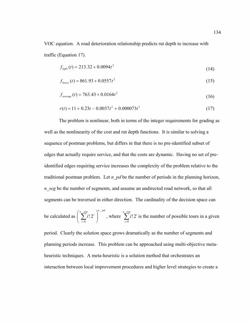
134 VOC equation. A road deterioration relationship predicts rut depth to increase with
traffic (Equation 17).
20094.032.213)( ttf light += (14)
20557.093.861)( ttf heavy += (15)
20164.043.763)( ttf average += (16)
32 000073.00037.023.011)( ttttr +−+= (17)
The problem is nonlinear, both in terms of the integer requirements for grading as
well as the nonlinearity of the cost and rut depth functions. It is similar to solving a
sequence of postman problems, but differs in that there is no pre-identified subset of
edges that actually require service, and that the costs are dynamic. Having no set of pre-
identified edges requiring service increases the complexity of the problem relative to the
traditional postman problem. Let n_pd be the number of periods in the planning horizon,
n_seg be the number of segments, and assume an undirected road network, so that all
segments can be traversed in either direction. The cardinality of the decision space can
be calculated as pdnsegn
i
ii__
02! ⎟⎟⎠
⎞⎜⎜⎝
⎛ ∑=
, where ∑=
segn
i
ii_
0
2! is the number of possible tours in a given
period. Clearly the solution space grows dramatically as the number of segments and
planning periods increase. This problem can be approached using multi-objective meta-
heuristic techniques. A meta-heuristic is a solution method that orchestrates an
interaction between local improvement procedures and higher level strategies to create a

135 process capable of escaping from local optima and performing a robust search of a
solution space (Glover and Kochenberger 2003).
4.4 Solution Method
We employed a multi-objective evolutionary algorithm (MOEA) to generate
solutions to this problem. MOEA’s are a popular tool for solving multi-objective routing
problems (Jozefowiez et al. 2008) and, more generally, multi-objective combinatorial
optimization problems (Ehrgott and Gandibleux 2000). In a survey of multi-objective
metaheuristic use, Jones et al. (2002) found that 94% of practitioners used some form of
an evolutionary algorithm. According to Zitzler et al. (2000, p. 173), evolutionary
algorithms “have become established as the method at hand for exploring the Pareto-
optimal front in multi-objective optimization problems that are too complex to be solved
by exact methods.”
Evolutionary algorithms mimic natural processes of biological evolution, in
particular the concept of natural selection. From a population of solutions, high quality
solutions are preferentially selected to mate, and these solutions are then stochastically
perturbed to create a new generation of solutions. Maintaining a population of solutions
is advantageous for multi-objective programming, as a single run of the algorithm can
generate multiple solutions along the efficient frontier. Retaining multiple solutions also
promotes diversity in the solution space.
There exist numerous MOEA approaches, though generally speaking there is no
algorithm that is superior for all problem types (Wolpert and Macready 1997), or across

136 all possible performance measures (Tan et al. 2002). That said, there are certain design
elements that have been shown to facilitate convergence and diversity, notably elitism
and fitness sharing (Van Veldhuizen and Lamont 2000). Elitism in particular is
important, as it is required to guarantee convergence of MOEA’s (Rudolph and Agapie
2000).
We opted to employ the Strength Pareto Evolutionary Algorithm (SPEA), which
employs both fitness sharing and elitism (Zitzler and Thiele 1999). In fact, SPEA is
considered a landmark in MOEA development because it formally introduced the elitist
notion of retaining an external population of non-dominated solutions (Coello Coello
2006). Fitness assignment proceeds according to two phases. In the first phase,
individuals in the external set are assigned a strength value that is proportional to the
number of individuals in the current population they dominate. Next, individuals in the
current population are assigned fitness values as the sum of the strengths of all external
solutions. Clustering is used to reduce the size of the number of non-dominated solutions
while preserving the essential characteristics of the tradeoff frontier, and a novel Pareto-
based niching method is employed to preserve diversity.
Comparative analyses have demonstrated that SPEA can produce high quality
solutions to multi-objective test problems. SPEA was found to efficiently guide the
search towards the Pareto-optimal front, and outperformed four other MOEA’s on 0/1
knapsack problems (Zitzler and Thiele 1999). Zitzler et al. (2000) evaluated eight
solution methods and identified SPEA as the best algorithm in terms of producing
solutions closest to the true Pareto front, citing elitism as an important factor in its

137 success. Tan et al. (2002) also reported good performance from SPEA, referring to
elitism and fitness sharing as important algorithm design features.
Zitzler et al. (2001) proposed an improved version, SPEA2, which was shown to
provide improved results over SPEA. Major differences in SPEA2 include a modified
fitness assignment scheme based on dominance relations between the population and the
archive, a new density estimation technique to facilitate clustering, and a new method for
truncating the elitist archive to preserve boundary solutions. Steps in the algorithm are
presented below (Zitzler et al. 2001, p. 5):
1. Initialization: Generate an initial population 0P and create the empty archive
(external set) ∅=0P . Set t = 0.
2. Fitness assignment: Calculate fitness values of individuals in tP and tP .
3. Environmental selection: Copy all non-dominated individuals in tP and tP to
1+tP . If size of 1+tP exceeds N then reduce 1+tP by means of the truncation
operator, otherwise if size of 1+tP is less than N then fill 1+tP with non-dominated
individuals in tP and tP .
4. Termination: If Tt ≥ or another stopping criterion is satisfied then set A to the set
of non-dominated individuals in 1+tP . Stop.
5. Mating selection: Perform binary tournament selection with replacement on
1+tP in order to fill the mating pool.

138
6. Variation: Apply recombination and mutation operators to the mating pool and
set 1+tP to the resulting population. Increment generation counter (t = t + 1) and
go to Step 2.
4.5 Algorithm Design
We represent solutions as chromosomes of length n, where n corresponds to the
number of periods in the planning horizon. Each gene in the chromosome in turn
represents a daily tour for the maintenance vehicle to take. As stated above, tours define
the order in which certain road segments are to be graded, and can vary in total number of
road segments serviced. Between solutions therefore, chromosome length but not gene
length are constant. In terms of data structures, this can easily be represented by an array
of pointers, with each pointer referencing a dynamically-sized array or linked list
corresponding to each tour.
With recombination solutions mate and exchange genetic information through a
process called crossover. Recombination is a stochastic procedure that promotes
diversity in the search process. Various implementations exist; based upon the initial
algorithm in Zitzler et al. (2001) we opted for a 1-point crossover, wherein a point in the
chromosome is randomly selected to act as a dividing point for the offspring. The first
offspring receives all the genes up through that point from one parent, and from the other
parent beyond that point. The second offspring similarly receives contiguous genetic
blocks, but from the opposite parents. In our implementation, sequences of daily tours
are swapped between offspring, but the tours themselves are not altered. We opted for a

139 recombination rate of 80% based upon previous implementations of SPEA (Zitzler et al.
2000; Zitzler and Thiele 1999).
Mutation is another diversity preserving mechanism, and serves to change the
genetic composition of solutions to that which could not be achieved through inheritance
alone. As we implemented it, mutation stochastically alters the tours themselves. Four
tour-changing operators are defined: add, remove, replace, and swap. Per mutation an
operator is randomly assigned, with each operator assigned an equal probability. The
“add” and “remove” operators increase/decrease the number of edges serviced on the
tour. “Replace” and “swap” instead rearrange a given tour, wherein either a new service
edge is inserted or the order of two existing edges rearranged.
We hypothesized that for our implementation it would be necessary to emphasize
the role of mutation, in order to facilitate exploration of individual tours. Mutation rates
for MOEAs typically range from 1% to 1/k, where k is the number of genes in a
chromosome (Tan et al. 2002; Knowles and Corne 2000; Zitzler et al. 2000; Zitzler and
Thiele 1999). Too low of a rate of mutation however may result in few additions,
removals, or permutations of service edges for individual tours beyond that generated
initially. We therefore experimented with mutation rates of 1%, 5%, 10%, 20%, 40%,
60%, and 80%. The concern that too high a mutation rate can effectively lead to pure
random search may be tempered in this context because of retention of the elitist archive
to populate subsequent generations. That is, the trajectory of the search isn’t determined
by the current population to which the mutation operator was just applied, but rather by
the archive.

140
The sizes of the population and in particular the archive can significantly impact
algorithm performance, and are therefore important design choices. Too small an archive
may not sufficiently span the objective space, but too large an archive increases
computational effort, which is of special concern here due to the complexity of the
SPEA2 archive truncation operator (Zitzler et al. 2001). In some studies the archive size
has been set to roughly a quarter of the population size (e.g., Tan et al. 2002; Zitzler et al.
2000; Zitzler and Thiele 1999), whereas others have used identical population and
archive sizes (e.g., Zitzler et al. 2001; Knowles and Corne 2000). Ultimately any size
chosen will reflect a compromise between solution quality (i.e., how closely the results
approximate the true Pareto frontier) and computational effort. After experimentation we
arrived at an archive size of 40% of the population size, where the population size
changes with the size of the problem being solved. Both the population and archive were
stored in a linear list per the recommendation of Mostaghim et al. (2002).
Prior to invoking the SPEA2 algorithm, the population is initialized according to a
semi-random procedure. First, solutions to the simulated policy scenarios are input.
These policies correspond to the practice of grading at fixed traffic intervals, and are
described in more detail in the following section. The rationale for doing so is that these
solutions may already lie near or along the Pareto frontier, and thus may be good starting
points for further exploration. For all subsequent solutions in the population, both the
number of service edges per period and the specific edges to be serviced in that period are
generated randomly. After initializing the population, we ran the algorithm for a total of
20,000 generations, a value arrived at after initial experimentation.

141
4.6 Example Applications
To demonstrate the utility of a planning approach based upon Pareto optimality,
we present results from two example applications. For both examples we use road
segment information obtained from the GIS database for the McDonald-Dunn Forest, a
research forest managed by the College of Forestry at Oregon State University. The first
case study, Example #1, is of moderate size (though the cardinality of the solution space,
as described above, is quite large), which we describe in detail for the benefit of the
interested reader. Example #1 extracts timber sale information from 3 planned sales
(Dave Lysne, College Forests Director, Oregon State University, personal
communication, August 2008), the traffic for which is routed across 9 road segments,
over a planning horizon of 22 periods. The second case study considers a larger 141-
edge network, using road data originally presented in Thompson et al. (2007), and
considers six hypothetical timber sales scheduled over a 20 period planning horizon.
Parameters relating to operation of the grader were estimated using data from
Provencher (1995). We assume an operating cost of $50/hr, and that the grader can
deadhead at 40 km/hr and grade at 5km/hr. Daily tour lengths are limited to 8 operating
hours. Feasibility is retained through the search by requiring feasibility as a precondition
for selection into the archive. In addition, the population initialization procedure only
adds segments to tours if doing so won’t result in an infeasible tour length.
Loaded log truck traffic was estimated assuming daily production levels of
~20mbf per timber sale. Each loaded log truck carries ~4mbf per load, and each

142 pickup/delivery requires two one-way trips. Associated light vehicle and rock haul traffic
were calculated using methods outlined above. Based on these regimes we calculated the
total number of loaded log trucks entering each segment for each period, as well as the
cumulative traffic volume (support vehicle, rock haul, timber haul) across each segment.
For simplicity we model grading to evenly split segment-level traffic. That is,
half of the traffic occurs before the segment is graded, and the remainder of traffic after
grading. Consider a single segment over the course of two periods, with 20 vehicles per
period, and assume the segment will be graded in both periods. The sequence of
threshold traffic levels in this scenario would be T = {10, 20, 10}. Because traffic levels
are consistent irrespective of tour ordering, rut depth calculations will not change in
response to a re-ordering of a given period’s tour. Rather, the total number of times each
segment is serviced and the associated inter-grading traffic levels influence rut depth
levels.
For purposes of comparison we simulate four alternative grading policies
representative of practices that are common within the forest industry (Provencher 1995).
Individual segments are assigned to be graded based upon cumulative timber volume haul
since the previous grading. Infrequent grading will lead to lower total costs at the
expense of higher hazard-weighted rut depth scores. We identified traffic thresholds
based upon cumulative timber volume levels of 0.5 MMBF, 1 MMBF, 1.5 MMBF, and 2
MMBF, which henceforth are referred to as Policy Solutions #1, #2, #3, and #4,
respectively. Service periods could then be calculated by overlaying the grading policy
on the cumulative traffic for each segment.

143
We used the MOEA to find efficient tours for each simulated grading policy,
given a fixed grading schedule as an initial solution. Because the traffic levels between
grading were fixed, and therefore rut depth fixed as well, the MOEA sought only to
rearrange daily tours so as to minimize total cost. To accomplish this we modified the
mutation procedure to only perform “replace” and “swap” operations. Any lower cost
solution by definition dominates in this context, and would therefore be updated into the
archive. We set the archive size to one, effectively rendering our MOEA a single-
objective evolutionary algorithm. Alternatively we could have opted to use tabu search,
which has demonstrated success for single objective routing problems (Thompson et al.
2007; Corberán et al. 2000; Hertz et al. 2000; Gendreau et al. 1994), but retained the
MOEA approach for consistency.
To compare algorithm performance across mutation rates we employ two
complementary metrics: size of the space covered (S) and coverage of two sets (C).
Returning to the formulations of Equations 1 and 2, let DxxxX r ⊆=′ )...,,,( 21 be a set
of r decision vectors. In our two-dimensional case, the function )(XS ′ calculates the
union of all rectangles defined by the points (0, 0) and (f1(xi), f2(xi)). Larger values of S
indicate broader coverage of the objective space, which is desirable. As an independent
measure of performance S is limited however, because it does not distinguish between
concave and convex regions in the objective space.
The second metric, C, indicates the degree to which the outcomes of one
algorithm dominate another algorithm, thereby overcoming the shortcoming of S.
Consider ., DXX ⊆′′′ The function ),( XXC ′′′ maps the order pair ),( XX ′′′ to the

144 interval [0, 1], where a value of 1 indicates that all points in X ′′ are dominated by or are
equal to (i.e., covered by) points in X ′ . A value of 0 indicates that none of the points in
X ′′ are covered by points in X ′ . In a pair-wise comparison of output from algorithms
(or, in our case, various mutation rates), we would clearly prefer solution X ′ to X ′′ when
),(),()()( XXCXXCXSXS ′′′≥′′′∩′′≥′ . Readers are referred to Zitzler and Thiele
(1999) for more detailed information on these metrics.
We developed our SPEA2 code in Microsoft Visual C++ 6.0. S values were
calculated using the polyarea() functionality of MATLAB, and C values were calculated
using a simple Visual Basic for Applications macro within Microsoft Excel. All results
presented below were generated on a HP Pavilion dv6000 laptop, which has a dual-core
2.2 GHz processor and 2GB DDR2 SDRAM.
Example #1
Figure 1 displays the road network and timber sales for Example #1. Estimated
timber volumes were 715 mbf, 1700 mbf, and 1300 mbf for the Bean, Berry, and
Racetrack sales, respectively. Traffic associated with these sales is routed over five roads
(R100, R140, R142, R190, and R1010), divided into a total of nine segments (R100.1,
R100.2, R100.3, R140.1, R140.2, R142.1, R190.1, R190.2, and R1010.1). The network
comprises a total of 11.00 km. Traffic regimes associated with each timber sale are
presented in Table 1. For each timber sale the log trucks’ routes over the network, as
identified by segment order, are presented. Each timber sale is modeled as having three
landings, and subsequently three different input segments.

145 Table 2 presents total traffic over each segment (in both directions), which includes light
support vehicles, rock haul, and log truck traffic. Road 100 is the mainline, and thus
aggregates the most traffic. The depot, the point to which the grader must return, is
assigned to the beginning of Road 100. Segment-level grading frequencies for each
simulated policy are presented in Table 3.
Table 4 presents S and C values for the various mutation rates we tested on
Example #1. Values used in S and C calculations represent the aggregated non-
dominated solutions from multiple runs of each mutation rate. We felt 30 runs were
sufficient to account for inherent stochastic variability (Zitzler and Thiele 1999). The
area of the objective space spanned (S) generally increases with the mutation rate,
although S for the 1% mutation rate is slightly larger than for rates of 5% and 10%.
Based on S alone, a mutation rate of 80% appears superior because its frontier spans the
largest area of objective space. This could suggest that higher mutation rates facilitate
additional exploration of individual (daily) tours, thereby exploring more of the objective
space to reach efficient boundary solutions. Alternatively, it could suggest that with
higher mutation rates the algorithm identifies a frontier with convex regions, which in
this dual-minimization case is undesirable. Figure 2, which displays the frontiers for
mutation rates of 1% and 80%, indicates in this instance that the latter is occurring.
Solutions generated using the higher mutation rate span more of the objective space,
especially the low rut-depth, high-cost region, but at the same time are dominated across
nearly the entire objective space.

146
Moving next to examine C values, our results indicate that lower mutation rates
outperform higher rates. The diagonal of the C matrix corresponds to the identity matrix,
because a solution (set of decision vectors) by definition covers itself. Above this
diagonal, coverage values range from 46-100%, demonstrating the better performance of
lower mutation rates. Below the diagonal coverage values are much lower. The non-
dominated frontier generated using a mutation rate of 5% covered (dominated or was
equal to) all other rates (i.e., DXXC ⊆′′∀=′′ 00.1)%,5( ). Thus there is a benefit to
expanding the search via higher mutation rates (relative to the more standard rate of 1%),
but only to a point. With significantly higher mutation rates the search does not converge
towards the Pareto frontier. Though this result is not unexpected, it would be premature
to conclude that higher mutation rates are always undesirable, as this is a relatively small
example where perhaps expansive exploration of each tour was unnecessary. Based upon
our results from Example #1, we opted to experiment with rates of 1%, 5%, 10%, 20%,
and 40% for the larger problem in Example #2.
Hazard weighted rut depth values ranged from 8.47 to 8.58 mm, where the latter
value corresponds to no grading at all. Note this metric is an integral of the aggregated
hazard weighted rut depth across all road segments; it does not reflect actual rut depth
values on any particular segment. Absent grading, we would expect a rut depth of ~11.5
mm for road segment 100.1 at the end of the planning horizon (see Equation 17). We
integrate over all days in the planning horizon to reflect our assumption of cumulative
environmental degradation associated with rutted road surfaces. Values for total cost
ranged from $6458 to $7842. Vehicle operating costs were relatively insensitive to

147 grading because of the small network and low traffic levels, and so most of the range in
cost variation stems from grader utilization.
Figure 3 presents the non-dominated frontier in relation to the four policy
solutions, represented as discrete points in the objective space. In total our MOEA
identified 111 non-dominated solutions. The policy corresponding to grading after 2
MMBF (Policy Solution #4) is the upper left policy solution in Figure 3. Progressing
along the frontier towards higher cost solutions leads to policies with progressively
smaller intervals between grading. Policy Solution #1 (0.5 MMBF) results in the best
environmental performance of the policy solutions. Beyond Policy Solution #1 there
appears to be decreasing marginal returns, suggesting monetary resources slated for
grading could be better utilized performing other maintenance operations.
Policy Solutions #1, #2, and #4 were each dominated by 1, 4, and 1 individual(s),
respectively. Policy Solution 3 was non-dominated. This suggests that, with this
network and traffic regime, the simulated management policies are efficient.
Example #2
Figure 5 displays the road network for the Dunn Forest managed by the College
of Forestry at Oregon State University, a portion of which is modeled for Example #2.
The network contains 127 nodes, 141 edges, and comprises a total of 72.27 km. Six
timber sales were simulated using values bounded by the range of the sales in Example
#1, and were scheduled to occur over a planning horizon of 20 periods. Table 5 presents
traffic regimes associated with each timber sale. Truck routing from timber sales results

148 in traffic across 67 segments, effectively reducing the size of the decision space (i.e.,
roads servicing no traffic were assumed to require no grading). Information on all road
segments needs to be retained however, as the algorithm routes the grader over shortest
paths between segments when deadheading. Appendix 1 presents segment-level
information for those segments over which traffic will flow.
Figure 6 compares the non-dominated frontier output by SPEA to simulated
policy solutions. A total of 152 non-dominated solutions were identified. All policy
simulations were dominated, indicating that the same level of environmental performance
(as measured by hazard weighted rut depth) can be achieved at lower overall total cost,
thereby freeing up resources for other road management activities. Alternatively, for the
same level of expenditure the environmental performance of the road network could be
improved.
Table 6 presents S and C values for various mutation rates tested in Example #2.
Here a mutation rate of 10% is clearly dominant, as it spans the largest region of the
objective space (S), and completely covers frontiers generated using other mutation rates
(C). Higher mutation rates performed better in Example #2 than in Example #1,
suggesting a positive association between mutation rate, problem size, and algorithm
performance. Our results also suggest a positive association between problem size and
coverage of policy solutions by the MOEA’s approximated Pareto frontier, though this
question is best answered by further experimentation.
Solution time increased dramatically from Example #1 to Example #2. This is
due to a combination of the larger road network and the larger respective archive and
149 population sizes. We used sizes of 100 and 40 for the population and archive,
respectively, for Example #1. For Example #2 we increased these values to 150 and 60,
respectively. Thus per generation the MOEA performed either 140 (Example #1) or 210
(Example #2) fitness evaluations. With Example #1 the MOEA iterated over an average
of 22.22 generations per second. With Example #2 algorithm speed dropped to 2.584
generations per second, nearly an order of magnitude lower. For much larger road
networks or much longer planning horizons, practitioners might want to consider
implementing the evolutionary algorithm in parallel to improve computational
performance (specifically, to speed up fitness evaluation). Of course reducing population
size and generation counts are also options, but generally come with the expectation of
worse solution quality.
4.7 Discussion
Forest road maintenance vehicle routing using the Pareto optimality approach
provides landowners with the opportunity to evaluate the economic and environmental
performance of their grading routing policies. Identifying more efficient grading routes
ideally results in a better-maintained road system. Cost-savings measures could release
resources for other road management activities, including those directed at reducing the
occurrence of ruts and other surface imperfections. This could entail reducing tire
pressure, changing traffic regimes, or strengthening the subgrade (Sessions et al. 2007).
Landowners may also wish to move along the non-dominated frontier towards grading

150 policies with better environmental performance, perhaps to achieve certification or
comply with regulatory requirements relating to water quality.
Efficient frontiers generated using the strength Pareto algorithm could be a
starting point for regulatory discussions regarding forest road management. Regulatory
frameworks, such as the Clean Water Act, often involve a balancing act between the cost
and benefit of any particular pollution control measure. The type of tradeoff analysis we
propose here informs landowners and regulators not only of what is possible, but of
where current management policies lie. If current policies comprise interior solutions
(i.e., they are dominated), there is clearly room for improvement. Alternatively,
landowners may demonstrate that their current practices are already efficient.
In our two examples we found that four simulated management policies based
upon cumulative timber-haul-related traffic were on or near the non-dominated frontier.
A primary benefit of identifying the frontier in this context is an improved understanding
of the environmental tradeoffs associated with scheduling grading according to various
traffic frequencies. Our results suggest that the marginal cost of achieving increasing
environmental performance beyond Policy Solution #1 (grade every 0.5 MMBF) can be
quite significant.
Certainly our results are in no small way artifacts of the particular cost and
environmental performance models used. The Faiz and Staffini (1979) study provided
published models for both vehicle operating cost and rut depth formation on low-volume
unpaved roads, which is scarce in the literature, and the Provencher (1995) study
provided a source for important parameters relating the operation of forest road
151 maintenance vehicles. The Faiz and Staffini (1979) study was particularly attractive for
our purposes because their work condensed the VOC equation to a function of a single
variable, cumulative traffic. In general, VOC is a function of multiple parameters
including climate, road geometry, road surfacing, and road surface deterioration. The
World Bank’s “Roads Software Tools” knowledge base is another source for VOC
models (http://www.worldbank.org/transport/roads/tools.htm), as is the National
Transportation Library (http://ntl.bts.gov/).
Forest landowners employing methods presented here may have alternate cost
models, different assumptions regarding grader operation, or may be more interested in
different measures of environmental performance. Another common metric to represent
road surface condition is roughness, often measured by the International Roughness
Index, a method employed by both Thompson et al. (2007) and Provencher (1995).
Alternatively other forms for measuring rut depth may be used. A model developed by
the U.S. Army Corps of Engineers (Barber et al. 1978) considers traffic, load, and road
surfacing parameters. Hazard factor calculations could be modified include additional
explanatory variables. We emphasized the importance of segment length, based upon
research by Foltz and Elliott (1998) citing flow path length as an important variable. Rut
length can interfere with the normal function of road shape and substantially increase
flow length. Slope along the flow path, water velocity, flow depth, and the detachability
of the road bed particles are known to affect sediment transport from the sediment
transport mechanics literature (Morris 1963). A stronger link is likely needed between

152 sediment, traffic, and road condition. We have bridged that gap using road deterioration
models predicting rut depth as a proxy.
4.8 Conclusion
Substantial sums are expended on gravel road maintenance throughout the world,
but there has been limited research directed towards systematically managing gravel
roads. Road maintenance and transport activities have been linked to sediment
production, but again, there has been limited research directed toward systematically
managing roads for sediment production. In the U.S., roads are receiving increasing
attention for their negative impacts on water quality, particularly relating to impacts on
fish. Although this attention has primarily been focused on forest lands, increasing
attention is being directed toward aggregate surfaced roads on non-forested lands as well.
We have brought together the ideas for managing roads to simultaneously minimize user
costs and environmental degradation associated with formation of ruts and other road
surface failures. Our examples have drawn coefficients from empirical results from the
literature. They are not intended to be handbook ready formulas, but are drawn from
specific studies and are intended to illustrate a conceptual system for approaching
aggregate road management.
We limited our discussion of road maintenance costs to grading. Surface rock
replacement is a function of traffic and could be considered a road maintenance activity.
We have assumed that rock replacement is a fixed cost and have not included it in the
objective function. If rock replacement is not directly proportional to total traffic, but is a

153 function of both grading schedule and traffic, then we could expand our maintenance cost
function to include it.
Future work in this area could focus on improving development of both the
solution algorithm and the operational model. Though solutions did appear to span large
regions of the objective space, it may be fruitful to consider using the notion entropy to
promote diversity along the non-dominated front (Farhang-Mehr and Azarm 2002). One
option mentioned earlier is to move to a parallel processing setup to speed up fitness
evaluations, and possibly to include much larger populations to offer a wider look into
the decision space. As we emphasized the role of mutation, considering other MOEAs
that focus on mutation could also be interesting. The Pareto Archived Evolution Strategy
of Knowles and Corne (2000), for instance, abandons recombination and only uses
mutation to introduce diversity into the solution space.
On the operational model side, there exists the possibility to employ alternate
models forms for both economic and environmental objectives. Perhaps most promising
would be the adoption of alternate equations to model rut depth formation. An equation
developed by the Army Corps of Engineers (Barber et al. 1978) and used by the U.S.
Forest Service for aggregate surface depth considers as input variables subgrade strength,
surface strength, tire pressure, and traffic. Using this equation would allow for rut depth
calculations more in line with what is expected for forest roads in the western U.S. The
model might also be expanded to incorporate log truck routing, or time windows during
which grading operations should not occur. Multiple maintenance vehicles and multiple
depots would be appropriate for larger networks.

154
Our results demonstrate the utility of using a multi-objective approach; using the
Strength Pareto Evolutionary Algorithm we were able to identify efficient solutions that
dominated simulated management policies in terms of economic and environmental
performance. Adoption of an a posteriori optimization approach should facilitate tradeoff
analysis and lead to informed compromise. Ultimately this manuscript demonstrates that
use of computerized decision aids could lead to increased efficiency when determining
routes for graders to take over a road network. The multi-objective programming
techniques we employed here could help landowners to “jointly produce”
environmentally benign, low-cost road networks. We hope this discussion will stimulate
additional research in road management of aggregate surfaced roads.

155 4.9 References
Aruga, K., Chung, W., Akay, A., Sessions, J., and E.S. Miyata. 2007. Incorporating Soil Surface Erosion Prediction into Forest Road Alignment Optimization, International Journal of Forest Engineering, 18(1), 24-32.
Barber, V.C., Odom, E.C., and R.W. Patrick. 1978. The deterioration and reliability of pavements. Technical Report S-78-8. U.S. Army Engineers Waterways Experiment Station, Vicksburg, Miss.
Boston, K., Pyles, M., and A. Bord. 2008. Compaction of Forest Roads in Oregon – Room for Improvement. International Journal of Forest Engineering 19(1): X-X.
Bettinger, P., Sessions, J., and K.N. Johnson. 1998. Ensuring the Compatibility of Aquatic Habitat and Commodity Production Goals in Eastern Oregon with a Tabu Search Procedure, Forest Science, 44(1), 96-112.
Bilby, R.E., K. Sullivan, and S.H. Duncan. 1989. The generation and fate of road- surface sediment in forested watersheds in southwestern Washington. Forest Science, 35(2), 453-468.
BLM 2003. The BLM Road Maintenance and Rock Wear Fees Calculation Handbook. Burroughs, E.R., Jr., and J.G. King. 1989. Reduction of soil erosion on forest roads,
General Technical Report INT-264. US Department of Agriculture, Forest Service, Intermountain Research Station, Ogden, UT, 21 pp.
Coello Coello, C.A. 2006. Evolutionary Multi-Objective Optimization: A Historical View of the Field. IEEE Computational Intelligence Magazine 1(1) : 28-36.
Coello Coello, C.A. 1999. An Updated Survey of Evolutionary Multiobjective Optimization Techniques: State of the Art and Future Trends. In, Proceedings of the 1999 Congress on Evolutionary Computation. Piscataway, N.J., 1999, pp. 3-13.
Corberán, A., Martí, R., and A. Romero. 2000. Heuristics for the Mixed Rural Postman Problem. Computers and Operations Research 27(2): 183-203.
Coulter, E.D., Sessions, J., and Wing, M.G. 2006. Scheduling Forest Road Maintenance Using the Analytic Hierarchy Process and Heuristics. Silva Fennica, 40(1), 143-160.
Dai, J.J., Lorenzato, S., and D.M. Rocke. 2004. A knowledge-based model of watershed assessment for sediment. Environmental Modelling and Software, 19(4), 423-433.
Eiselt, H.A., Gendreau, M., and G. Laporte. 1995. Arc Routing Problems, Part II: The Rural Postman Problem, Operations Research 43(3): 399-414.
Environmental Protection Agency. 1999. Protocol for Developing Sediment TMDL’s. First Edition. October 1999.
Ehrgott, M., and X. Gandibleux. 2000. A survey and annotated bibliography of multiobjective combinatorial optimization. OR Spektrum 22: 425-460.
Faiz, A., and E. Staffini. 1979. Engineering economics of the maintenance of earth and gravel roads. In, Proceedings of the Second International Conference on Low-Volume Roads, Transportation Research Record 702, TRB. P. 260-268.

156 Farhang-Merh, A., and S. Azarm. 2002. Diversity Assessment of Pareto Optimal Sets:
An Entropy Approach. In: Proceedings of the 2002 Congress on Evolutionary Computation, Honolulu, HI, May, 2002.
Foltz, R.B., and W.J. Elliot. 1998. Measuring and modeling impacts of tyre pressure on road erosion. In, Proceedings of the Seminar on Environmentally Sound Forest Roads and Wood Transport, Sinaia, Romania, FAO, Rome, pp. 205-214. http://www.fao.org/docrep/X0622E/X0622E00.htm
Gendreau, M., Hertz, A., and G. Laporte. 1994. A Tabu Search Heuristic for the Vehicle Routing Problem. Management Science 40(10): 1276-1290.
Girvetz, E. and Shilling, F. (2003), Decision Support for Road System Analysis and Modification on the Tahoe National Forest, Environmental Management, 32(2), 218-23.
Glover, F., and G. Kochenberger. 2003. Handbook of Metaheuristics. Kluwer Publishers. 556 p.
Gucinski H., Furniss M.J., Ziemer R.R., and M.H. Brookes (Eds.) 2001. Forest roads: a synthesis of scientific information. General Technical Report PNW-GTR-509. Portland, OR: US Department of Agriculture, Forest Service, Pacific Northwest Research Station.
Hide, H. 1975. Investigation of vehicle operating costs in Kenya. Low Volume Roads, Special Report 160, Transportation Research Board, National Research Council, National Academy of Sciences, Washington DC. P. 355-375.
Hertz, A., Laporte, G., and M. Mittaz. 2000. A Tabu Search Heuristic for the Capacitated Arc Routing Problem. Operations Research 48(1): 129-135.
Jones, D.F., Mirrazavi, S.K., and M. Tamiz. 2002. Multi-objective meta-heuristics: An overview of the current state-of-the-art. European Journal of Operational Research 137(1): 1-9.
Jozefowiez, N., Semet, F., and E. Talbi. 2008. Multi-objective vehicle routing problems. European Journal of Operational Research 189(2): 293-309.
Kennedy, M.C., Ford, D.E., Singleton, P., Finney, M., and J.K. Agee. 2008. Informed multi-objective decision-making in environmental management using Pareto optimality, Journal of Applied Ecology, 45(1), 181-192.
Knowles, J.D., and D.W. Corne. 2000. Approximating the Nondominated Front Using the Pareto Archived Evolution Strategy. Evolutionary Computation 8(2): 149-172.
Luce, C.H., and T.A. Black. 1999. Sediment production from forest roads in western Oregon. Water Resour. Res., 35(8), 2561-2570.
Luce, C.H., and T.A. Black. 2001. Effects of traffic and ditch maintenance on forest road sediment production, Proceedings of the Seventh Federal Interagency Sedimetation Conference, V-67 - V-74, U.S. Inter-agency Committee on Water Resources, Subcommittee on Sedimentation, Washington, D.C.
Madej, M.A., E.A. Eschenbach, C. Diaz, R. Teasley, and K. Baker. 2006. Optimization strategies for sediment reduction practices on roads in steep, forested terrain, Earth Surface Processes and Landforms, 31(13), 1643-1656.

157 Morris, H. 1963. Applied hydraulics in engineering. Ronald Press, NY. 455p. Mostaghim, S., Teich, J., and A. Tyagi. 2002. Comparison of data structures for storing
Pareto-sets in MOEAs. In, Proceedigns of the 2002 Congress on Evolutionary Computation, Part of the 2002 IEEE World Congress on Computational Intelligence, Hawaii. Piscataway, NJ: IEEE Press, May 12-17, 2002.
Provencher, Y. 1995. Optimizing Road Maintenance Intervals. Proceedings of the Sixth International Conference on Low-Volume Roads, Volume I, Minneapolis, MN, June 25-29, 1995. pp. 199-207.
Rackley, J. and W. Chung (2008), Incorporating Forest Road Erosion into Forest Resource Transportation Planning: A Case Study in the Mica Creek Watershed in Northern Idaho, Transactions of the ASABE, 51(1), 115-127.
Reid, L.M., and T. Dunne (1984), Sediment Production from Forest Road Surfaces, Water Resources Research, 20(11), 1753-1761.
Rudolph. G. and A. Agapie. 2000. Convergence properties of some multi-objective evolutionary algorithms,” In Proceedings of the 2000 Conference on Evolutionary Computation, vol. 2, pp. 1010–1016, Piscataway, New Jersey, IEEE Press, July 2000.
Sessions J., Boston, K., Wing, M., Akay, A., Theisen, P., and R. Heinrich. 2007. Forest Roads Operations in the Tropics. Springer. 170p.
Stückelberger, J.A., Heinimann, H.R., Chung, W., and M. Ulber (2006), Automatic road- network planning for multiple objectives. Proceedings of the 29th Council on Forest Engineering Conference, edited by W. Chung and H.S. Han, pp. 233-248, Council on Forest Engineering, Coeur d’Alene, ID.
Tan, K.C., Lee, T.H., and E.F. Khor. 2002. Evolutionary Algorithms for Multi- Objective Optimization: Performance Assessments and Comparisons. Artificial Intelligence Review 17(4): 253-290.
Toth, S.F., M.E. McDill, and S. Rebain. (2006), Finding the Efficient Frontier of a Bi- Criteria, Spatially Explicit, Harvest Scheduling Model, Forest Science, 52(1), 93-107.
Thompson, M., Sessions, J., Boston, K., Skaugset, A., and D. Tomberlin. 2008. Forest Road Erosion Control Using Pareto Optimality (In Review).
Thompson, M. and J. Sessions. (2008), Optimal Policies for Aggregate Recycling from Decommissioned Forest Roads, Environmental Management, 42(2), 297-309.
Thompson, M., Boston, K., Arthur, J., and J. Sessions. (2007), Intelligent Deployment of Forest Road Graders, International Journal of Forest Engineering, 18(2), 15-23.
Veldhuizen, D.A., and G.B. Lamont. 2000. Multiobjective Evolutionary Algorithms: Analyzing the State-of-the-Art. Evolutionary Computation 8(2): 125-147.
Wolpert, D.H., and W.G. Macready. 1997. No Free Lunch Theorems for Optimization. IEEE Transactions on Evolutionary Computation 1(1): 67-82.
Zitzler, E., Laumanns, M., and L. Thiele. 2001. SPEA2: Improving the Strength Pareto Evolutionary Algorithm. In K. Giannakoglou et al., editor, EUROGEN 2001. Evolutionary Methods for Design, Optimization and Control with Applications to Industrial Problems, pp. 95–100, Athens, Greece, 2002.

158 Zitzler E, Laumanns M, Thiele L. SPEA2: improving the strength Pareto evolutionary
algorithm. Tech Rep TIK-103, Department of Electrical Engineering, Swiss Federal Institute of Technology, 2001.
Zitzler, E., K. Deb, and L. Thiele. 2000. Comparison of Multiobjective Evolutionary Algorithms: Empirical Results. Evolutionary Computation 8(2): 173-195.
Zitzler, E., and L. Thiele. 1999. Multiobjective Evolutionary Algorithms: A Comparative Case Study and the Strength Pareto Approach. IEEE Transactions on Evolutionary Computation 3(4): 257-271.

159 Figure 4.1: Road network for Example #1. Shaded areas represent the various
timber sales scheduled for the 2009 season. The light gray stands represent the
Bean sale, cross-hatched stands represent the Berry sale, and shaded stands the
Racetrack sale.

160 Figure 4.2: Non-Dominated Frontier, Mutation Rates = 1% and 80%, Example #1.
This figure provides a comparison of non-dominated frontiers generated using
mutation rates of 1% and 80%. Total cost is defined as the sum of vehicle operating
cost and maintenance (grading) costs. The non-dominated frontier generated using
a mutation rate of 1% covered (dominated or was equal to) 98% of solutions
generated with a mutation rate of 80%. This figure demonstrates that spanning a
larger region of the objective space (as measured by S) it is not necessarily
preferable.

161 Figure 4.3: Non-Dominated Frontier (NDF) vs. Simulated Policy Solutions,
Example #1. This figure provides a comparison of non-dominated frontier against
simulated policy solutions, Example #1. Policy Solution #4 (grade every 2 MMBF) is
the upper left solution. Infrequent grading leads to lower total costs at the expense
of higher hazard-weighted rut depth scores. Progressing along the frontier towards
higher cost solutions leads to policy solutions associated with more frequent
grading. As expected, Policy Solution #1 (0.5 MMBF) results in the highest overall
cost and the best environmental performance of the policy scenarios. These results
suggest that the marginal cost of improving environmental performance beyond
Policy Solution #1 can be quite significant.

162 Figure 4.4: Non-Dominated Frontier (NDF) vs. Simulated Policy Solutions,
Example #1. This figure provides a close-up of non-dominated frontier in region of
objective space spanned by simulated policy objectives, Example #1. Though three
of four policy simulations were dominated, all were near the non-dominated frontier
for the network and traffic regime under consideration (i.e., the policy solutions are
efficient).

163 Figure 4.5: Road network for Example #2. Our graph representation contains 127
nodes and 141 undirected edges, and was originally used as a dataset by Thompson
et al. (2007). Roads included in the forest ownership and modeled here are
highlighted in bold. Other roads are presented in gray, as are stand boundaries.

164 Figure 4.6: Non-Dominated Frontier (NDF) vs. Simulated Policy Solutions,
Example #2. This figure provides a comparison of non-dominated frontier against
simulated policy solutions, Example #2. All policy simulations are dominated by the
frontier. That is, for a given level of total cost, it is possible to improve
environmental performance relative to the simulated policy. As with Example #1,
we see a steep decrease in cost/benefit ratio beyond Policy #4.

165 Table 4.1: Loaded Log Truck Traffic Regimes, Arranged by Timber Sale, Example
#1. For each timber sale the log trucks’ routes over the network, as identified by
segment order, are presented. Each timber sale is modeled as having three landings,
and subsequently three different input segments. The right column indicates the
number of loads (4mbf / load) and the periods corresponding to each landing
serving each timber sale.
Bean (179 loads; Pds 1-10):
190.2 → 190.1 → 100.3 → 100.2 → 100.1 (60 loads; Pds 1-3)
190.1 → 100.3 → 100.2 → 100.1 (60 loads; Pds 4-6)
1010.1 → 100.1 (59 loads; Pds 7-10)
Berry (425 loads; Pds 1-22):
142.1 → 140.1 → 100.2 → 100.1 (142 loads; Pds 1-8)
140.2 → 140.1 → 100.2 → 100.1 (142 loads; Pds 8-15)
100.2 → 100.1 (141 loads; Pds 15-22)
Racetrack (325 loads; Pds 3-19):
100.3 → 100.2 → 100.1 (109 loads; Pds 3-8)
100.2 → 100.1 (108 loads; Pds 8-13)
1010.1 → 100.1 (108 loads; Pds 13-19)

166 Table 4.2: Total Traffic (Light Vehicle, Rock Haul, Log Truck) over all Road
Segments, Example #1. Roundtrip traffic levels are provided. Road 100 is a
mainline and hence accumulates the most traffic.
Period Road Segment
100.1 100.2 100.3 140.1 140.2 142.1 190.1 190.2 1010.1
1 99 99 50 50 0 50 50 50 0
2 99 99 50 50 0 50 50 50 0
3 149 149 99 50 0 50 50 50 0
4 149 149 99 50 0 50 50 0 0
5 149 149 99 50 0 50 50 0 0
6 149 149 99 50 0 50 50 0 0
7 99 50 0 50 0 50 0 0 50
8 149 99 22 50 45 5 0 0 50
9 146 99 0 50 50 0 0 0 47
10 99 99 0 50 50 0 0 0 0
11 99 99 0 50 50 0 0 0 0
12 99 99 0 50 50 0 0 0 0
13 99 94 0 50 50 0 0 0 5
14 99 50 0 50 50 0 0 0 50
15 99 50 0 10 10 0 0 0 50
16 99 50 0 0 0 0 0 0 50
17 99 50 0 0 0 0 0 0 50
18 99 50 0 0 0 0 0 0 50
19 64 50 0 0 0 0 0 0 15
20 50 50 0 0 0 0 0 0 0
21 50 50 0 0 0 0 0 0 0
22 15 15 0 0 0 0 0 0 0

167 Table 4.3: Segment-level grading frequency for each simulated management policy,
Example #1. Cumulative traffic levels associated with each level of cumulative
timber haul were overlaid with the simulated grading policies to identify service
periods for each road segment. The modified single-objective evolutionary
algorithm was then invoked to identify efficient (minimal cost) individual tours
prior to passing these solutions into SPEA. For the largest (2 MMBF) threshold
only segments along the mainline (Road 100) are scheduled for grading, and then
only once over the planning horizon.
Segment Service Periods, arranged by simulated management policy
P1 (0.5 MMBF) P2 (1.0 MMBF) P3 (1.5 MMBF) P4 (2.0 MMBF)
100.1 4, 7, 8, 14, 18 6, 12, 19 8, 18 11
100.2 4, 7, 9 6, 14 9 12
100.3 5, 16 - - -
140.1 7, 14 14 -
140.2 10 - - -
142.1 7 - - -
190.1 - - - -
190.2 - - - -
1010.1 17 - - -
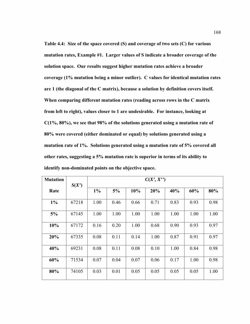
168 Table 4.4: Size of the space covered (S) and coverage of two sets (C) for various
mutation rates, Example #1. Larger values of S indicate a broader coverage of the
solution space. Our results suggest higher mutation rates achieve a broader
coverage (1% mutation being a minor outlier). C values for identical mutation rates
are 1 (the diagonal of the C matrix), because a solution by definition covers itself.
When comparing different mutation rates (reading across rows in the C matrix
from left to right), values closer to 1 are undesirable. For instance, looking at
C(1%, 80%), we see that 98% of the solutions generated using a mutation rate of
80% were covered (either dominated or equal) by solutions generated using a
mutation rate of 1%. Solutions generated using a mutation rate of 5% covered all
other rates, suggesting a 5% mutation rate is superior in terms of its ability to
identify non-dominated points on the objective space.
Mutation
Rate S(X’)
C(X’, X’’)
1% 5% 10% 20% 40% 60% 80%
1% 67218 1.00 0.46 0.66 0.71 0.83 0.93 0.98
5% 67145 1.00 1.00 1.00 1.00 1.00 1.00 1.00
10% 67172 0.16 0.20 1.00 0.68 0.90 0.93 0.97
20% 67335 0.08 0.11 0.14 1.00 0.87 0.91 0.97
40% 69231 0.08 0.11 0.08 0.10 1.00 0.84 0.98
60% 71534 0.07 0.04 0.07 0.06 0.17 1.00 0.98
80% 74105 0.03 0.01 0.05 0.05 0.05 0.05 1.00

169 Table 4.5: Loaded Log Truck Traffic Regimes, Arranged by Timber Sale, Example
#2. For brevity we do not display all routes for all respective input segments
(landings), as we do in Table #1. Rather, we display the input segments as well as
their common route to the depot. Segments in parentheses indicate different initial
routes to the common route. The first node of segment 0 represents the depot, to
which the grader must return at the end of each tour.
Timber Sale #1 (200 loads, Pds 1-10):
Input Segments: 8, 54, 55
8 → 6 → 2 → 0
Timber Sale #2 (300 loads, Pds 6-20):
Input Segments: 46, 47, 50
50 → 104 → 101 → 99 → 98 → 16 → 12 → 14 → 11 → 4 → 1 → 0
Timber Sale #3 (300 loads; Pds 4-18):
Input Segments: 140, 139, 138
(130, 138) → 132 → 133 → 134 → 137 → 52 → 51 → 128 → 53 → 7 → 5 → 2 → 0
Timber Sale #4 (300 loads; Pds 2-16):
Input Segments: 84, 85, 88
88→ 90 → 48 → 49 → 93 → 95 → 97 → 98 → 16 → 12 → 14 → 1 → 0
Timber Sale #5 (400 loads; Pds 1-20):
Input Segments: 122, 123, 124
122→ 120 → 119 → 118 → 116 → 112 → 107 → 102 → 96 → 92 → 91 → 49 → 93 →
95 → 97 → 98 → 16 → 12 → 14 → 11 → 4 → 1 → 0
Timber Sale #6 (200 loads; Pds 11-20):
Input Segments: 57, 58, 59
59→ 60 → 61 → 63 → 67 → 76 → 79 → 80 → 81 → 89 → 90 → 48 →49 → 93 → 95 →
97 → 98 → 16 → 12 → 14 → 11 → 4 → 1 → 0

170 Table 4.6: Size of the space covered (S) and coverage of two sets (C) for various
mutation rates, Example #2. Here a mutation rate of 10% is clearly dominant, as it
spans the largest region of the objective space (S), and completely covers frontiers
generated using other mutation rates (C). Higher mutation rates performed better
in Example #2 than in Example #1, suggesting a positive association between
mutation rate and problem size.
Mutation
Rate S(X’)
C(X’, X’’)
1% 5% 10% 20% 40%
1% 822689 1.00 0.44 0.21 0.18 0.52
5% 826815 0.25 1.00 0.19 0.15 0.42
10% 827039 1.00 1.00 1.00 1.00 1.00
20% 825731 0.50 0.38 0.26 1.00 0.66
40% 817132 0.13 0.28 0.19 0.08 1.00

171 Appendix 4.1: Listing of input segment-level input data for Example #2, Oregon
State Research Forest planning example. For brevity data is presented in comma-
delimited format. Data is presented according to the format: segment ID, node 1,
node 2, distance, and cumulative traffic in periods 1-20.
0,0,1,1536.16713,99,149,149,198,198,248,248,248,248,248,248,248,248,248,248,248,198,198,149,149 1,1,2,1094.55235,50,99,99,99,99,149,149,149,149,149,198,198,198,198,198,198,149,149,149,149 2,1,3,224.89367,50,50,50,99,99,99,99,99,99,99,50,50,50,50,50,50,50,50,0,0 3,2,6,157.18054,50,99,99,99,99,149,149,149,149,149,198,198,198,198,198,198,149,149,149,149 4,3,4,2469.21762,0,0,0,50,50,50,50,50,50,50,50,50,50,50,50,50,50,50,0,0 5,3,5,668.45786,50,50,50,50,50,50,50,50,50,50,0,0,0,0,0,0,0,0,0,0 6,4,38,410.2114,0,0,0,50,50,50,50,50,50,50,50,50,50,50,50,50,50,50,0,0 7,5,39,291.70943,50,50,50,50,50,50,50,50,50,50,0,0,0,0,0,0,0,0,0,0 8,6,98,8.97443,50,99,99,99,99,149,149,149,149,149,198,198,198,198,198,198,149,149,149,149 9,7,8,1889.44167,50,99,99,99,99,149,149,149,149,149,198,198,198,198,198,198,149,149,149,149 10,7,98,1164.84609,50,99,99,99,99,149,149,149,149,149,198,198,198,198,198,198,149,149,149,149 11,8,80,2333.61589,50,99,99,99,99,149,149,149,149,149,198,198,198,198,198,198,149,149,149,149 12,32,33,903.26212,0,0,0,0,0,50,50,50,50,50,0,0,0,0,0,0,0,0,0,0 13,33,36,49.97247,0,0,0,0,0,50,50,50,50,50,50,50,50,50,50,0,0,0,0,0 14,35,71,1557.58417,0,50,50,50,50,50,50,50,50,50,99,99,99,99,99,99,50,50,50,50 15,35,73,207.20167,50,99,99,99,99,99,99,99,99,99,149,149,149,149,149,149,99,99,99,99 16,36,87,31.12595,0,0,0,0,0,50,50,50,50,50,50,50,50,50,50,50,50,50,50,50 17,37,112,2288.80415,0,0,0,50,50,50,50,50,50,50,50,50,50,50,50,50,50,50,0,0 18,37,119,291.60221,0,0,0,50,50,50,50,50,50,50,50,50,50,50,50,50,50,50,0,0 19,38,111,913.74513,0,0,0,50,50,50,50,50,50,50,50,50,50,50,50,50,50,50,0,0 20,39,40,2119.78581,0,0,0,0,50,50,50,50,0,0,0,0,0,0,0,0,0,0,0,0 21,39,41,290.18548,50,50,50,50,0,0,0,0,0,0,0,0,0,0,0,0,0,0,0,0 22,43,44,73.63756,0,0,0,0,0,0,0,0,0,0,50,50,50,50,0,0,0,0,0,0 23,44,45,38.28541,0,0,0,0,0,0,0,0,0,0,50,50,50,50,50,50,50,50,0,0 24,45,46,1417.03203,0,0,0,0,0,0,0,0,0,0,50,50,50,50,50,50,50,50,50,50 25,46,47,2664.23705,0,0,0,0,0,0,0,0,0,0,50,50,50,50,50,50,50,50,50,50 26,47,48,7.8559,0,0,0,0,0,0,0,0,0,0,50,50,50,50,50,50,50,50,50,50 27,48,51,210.49096,0,0,0,0,0,0,0,0,0,0,50,50,50,50,50,50,50,50,50,50 28,51,58,5522.03476,0,0,0,0,0,0,0,0,0,0,50,50,50,50,50,50,50,50,50,50

172 29,58,63,3747.51272,0,0,0,0,0,0,0,0,0,0,50,50,50,50,50,50,50,50,50,50 30,61,63,209.04659,0,0,0,0,0,0,0,0,0,0,50,50,50,50,50,50,50,50,50,50 31,61,62,410.37684,0,0,0,0,0,0,0,0,0,0,50,50,50,50,50,50,50,50,50,50 32,62,69,2697.1344,0,0,0,0,0,0,0,0,0,0,50,50,50,50,50,50,50,50,50,50 33,65,66,352.80896,0,50,50,50,50,50,0,0,0,0,0,0,0,0,0,0,0,0,0,0 34,66,68,1348.03481,0,50,50,50,50,50,50,50,50,50,50,0,0,0,0,0,0,0,0,0 35,68,70,204.77576,0,50,50,50,50,50,50,50,50,50,50,50,50,50,50,50,0,0,0,0 36,69,70,101.63879,0,0,0,0,0,0,0,0,0,0,50,50,50,50,50,50,50,50,50,50 37,70,71,2338.26735,0,50,50,50,50,50,50,50,50,50,99,99,99,99,99,99,50,50,50,50 38,72,73,243.18422,50,50,50,50,50,50,50,50,50,50,50,50,50,50,50,50,50,50,50,50 39,72,76,5820.27941,50,50,50,50,50,50,50,50,50,50,50,50,50,50,50,50,50,50,50,50 40,73,75,2310.62351,50,99,99,99,99,99,99,99,99,99,149,149,149,149,149,149,99,99,99,99 41,75,77,767.64464,50,99,99,99,99,99,99,99,99,99,149,149,149,149,149,149,99,99,99,99 42,76,82,975.74585,50,50,50,50,50,50,50,50,50,50,50,50,50,50,50,50,50,50,50,50 43,77,78,375.61719,50,99,99,99,99,99,99,99,99,99,149,149,149,149,149,149,99,99,99,99 44,78,80,561.65708,50,99,99,99,99,149,149,149,149,149,198,198,198,198,198,198,149,149,149,149 45,78,79,136.29895,0,0,0,0,0,50,50,50,50,50,50,50,50,50,50,50,50,50,50,50 46,79,83,783.67796,0,0,0,0,0,50,50,50,50,50,50,50,50,50,50,50,50,50,50,50 47,82,85,1385.74306,50,50,50,50,50,50,50,50,50,50,50,50,50,50,50,50,50,50,50,50 48,83,87,1319.08812,0,0,0,0,0,50,50,50,50,50,50,50,50,50,50,50,50,50,50,50 49,85,92,688.56029,50,50,50,50,50,50,50,50,50,50,50,50,50,50,50,50,50,50,50,50 50,92,97,841.88716,50,50,50,50,50,50,50,50,50,50,50,50,50,50,50,50,50,50,50,50 51,97,100,1355.97638,50,50,50,50,50,50,50,50,50,50,50,50,50,50,50,50,50,50,50,50 52,100,103,1959.79864,50,50,50,50,50,50,50,50,50,50,50,50,50,50,50,50,50,50,50,50 53,102,103,213.76723,50,50,50,50,50,50,50,50,50,50,50,50,50,50,50,50,50,50,50,50 54,102,104,1010.34702,50,50,50,50,50,50,50,50,50,50,50,50,50,50,50,50,50,50,50,50 55,104,105,1172.89201,50,50,50,50,50,50,50,50,50,50,50,50,50,50,50,50,50,50,50,50 56,105,106,1148.15668,50,50,50,50,50,50,50,50,0,0,0,0,0,0,0,0,0,0,0,0 57,105,107,2201.59935,0,0,0,0,0,0,0,0,50,50,50,50,50,50,50,50,0,0,0,0 58,111,112,286.77853,0,0,0,50,50,50,50,50,50,50,50,50,50,50,50,50,50,50,0,0 59,114,122,774.11789,0,0,0,50,50,50,50,50,50,50,50,50,50,0,0,0,0,0,0,0 60,115,118,1479.97713,0,0,0,50,50,50,50,50,50,50,50,50,50,50,50,50,50,50,0,0 61,115,116,283.80169,0,0,0,50,50,50,50,50,50,50,50,50,50,50,50,50,50,50,0,0 62,116,117,752.55686,0,0,0,50,50,50,50,50,50,50,50,50,50,50,50,50,50,50,0,0 63,117,119,962.93952,0,0,0,50,50,50,50,50,50,50,50,50,50,50,50,50,50,50,0,0 64,118,124,17.87732,0,0,0,0,0,0,0,0,0,0,0,0,0,50,50,50,50,50,0,0 65,122,125,187.7666,0,0,0,50,50,50,50,50,50,50,50,50,50,0,0,0,0,0,0,0 66,125,126,8.67252,0,0,0,50,50,50,50,50,0,0,0,0,0,0,0,0,0,0,0,0

173
OPTIMAL POLICIES FOR AGGREGATE RECYCLING FROM
DECOMMISSIONED FOREST ROADS
Matthew P. Thompson
John Sessions
Environmental Management
Springer New York
Issue 42, Volume 2; Pages 297-309

174 5 Optimal Policies for Aggregate Recycling from Decommissioned Forest Roads
5.1 Abstract
To mitigate the adverse environmental impact of forest roads, especially
degradation of endangered salmonid habitat, many public and private land managers in
the western United States are actively decommissioning roads where practical and
affordable. Road decommissioning is associated with reduced long-term environmental
impact. When decommissioning a road it may be possible to recover some aggregate
(crushed rock) from the road surface. Aggregate is used on many low volume forest
roads to reduce wheel stresses transferred to the subgrade, reduce erosion, reduce
maintenance costs, and improve driver comfort. Previous studies have demonstrated the
potential for aggregate to be recovered and used elsewhere on the road network, at a
reduced cost compared to purchasing aggregate from a quarry. This paper investigates
the potential for aggregate recycling to provide an economic incentive to decommission
additional roads by reducing transport distance and aggregate procurement costs for other
actively used roads. Decommissioning additional roads may in turn result in improved
aquatic habitat. We present real-world examples of aggregate recycling and discuss the
advantages of doing so. Further, we present mixed integer formulations to determine
optimal levels of aggregate recycling under economic and environmental objectives.
Tested on an example road network, incorporation of aggregate recycling demonstrates
substantial cost-savings relative to a baseline scenario without recycling, increasing the
likelihood of road decommissioning and reduced habitat degradation. We find that

175 aggregate recycling can result in up to 24% in cost savings (economic objective) and up
to 890% in additional length of roads decommissioned (environmental objective).
5.2 Introduction
Public and private land managers in the western United States are increasingly
removing forest roads to mitigate negative environmental impacts associated with the
presence of roads on the landscape. The USDA Forest Service’s Road Management
Policy, for instance, states the agency’s intent to “reverse adverse ecological impacts
associated with roads” by, in part, “decommissioning unnecessary and unclassified
roads.” (USDA 2001) Other federal agencies have also sought to decommission roads
for ecological reasons, such as the USDI National Park Service within Redwood National
Park in 1978 (Madej 2001). Some private land managers are seeking to remove roads to
restore ecosystems, such as the Nature Conservancy’s Ellsworth Creek project (Tom
Kollasch, project manager, personal communication). Though roads provide many
benefits such as access for timber extraction, fire prevention, recreation and research,
roads can also adversely influence hydrology, geomorphology, and ecosystem processes
(Switalski et al. 2004). Road decommissioning has been identified as a pro-active
mechanism for preventing future habitat degradation and increasing the likelihood of
endangered salmonid survival (Harr and Nichols 1993).
Forest roads are associated with accelerated erosion and can be a major source of
sediment delivery to streams, which can degrade aquatic ecosystems (Jones et al. 2000;
Lugo and Gucinski 2000; Forman and Alexander 1998). Chronic erosion contributes fine

176 sediment and is generated by surface erosion processes along the road prism (Reid and
Dunne, 1984). Episodic erosion occurs in the form of mass-wasting and fluvial erosion
due to culvert failures and is often triggered by intense rain events (Reid and Dunne,
1984). Roads have been found to contribute as much as 40% of the total erosion
associated with forest management activities (Gucinski et al. 2001) and are responsible
for the majority of episodic erosion events such as hillslope failures in steep forested
areas subject to logging (Furniss et al. 1991). Elevated levels of in-stream sediment can
negatively affect salmonids through mortality, reduced growth rates, disruption of egg
and larvae development, and reduction in available food (Newcombe and MacDonald
1991; Hicks et al. 1991). Degradation of aquatic habitat is of special concern in the
western United States where endangered salmonid species spawn and rear in watersheds
containing potentially erosive forest roads.
Appropriate road management can mitigate the environmental impact of the road
system by limiting chronic erosion and reducing the risk associated with large-scale
episodic events (Weaver and Hagans 1999). Roads no longer required for transportation
can be closed and/or decommissioned. High maintenance needs or high levels of
environmental damage are also reasons to decommission a road. Closing a road
frequently consists of barricading or gating the road to prevent unauthorized use,
particularly during wet seasons, outsloping the surface and installing rolling dips and/or
waterbars, and may involve removing some high-risk culverts. A closed road can be re-
opened for future use or later decommissioned, and generally requires only periodic
inspection. Decommissioning a road may involve removing culverts under significant

177 fills, ripping the roadbed, recontouring hillslopes, and may include planting or seeding
the road surface. A decommissioned road is not passable and requires no future
maintenance. A common goal of decommissioning is to restore the natural hydrologic
processes and prevent future sedimentation; a decommissioned road has lower longer-
term environmental impacts than a closed road due to significantly reduced risk of
chronic and episodic erosion (Switalski et al. 2004; Kolka et al. 2004; Madej 2001;
Trombulak et al. 2000; Weaver and Hagans 1999; Harr and Nichols 1993).
Unfortunately decommissioning costs can be high and that may prevent desirable
projects from being undertaken. This is especially true with federal agencies such as the
USDA Forest Service, which has a minimal road maintenance budget due in large part to
substantial reductions in their timber sale program. Forest road networks under federal
ownership are often characterized by sub-standard conditions. As of 2002 less than
twenty percent of national forest roads were maintained to planned safety and
environmental standards (USDA 2002). A recent report from the Pinchot Institute for
Conservation found that four of five case study national forests (Allegheny (PA),
Chequamegon-Nicolet (WI), Fremont-Winema (OR) and Mt. Hood (OR)) had a backlog
of road maintenance and decommission needs, stating that there were “…some or, in
other cases, numerous inadequately maintained roads, many of which are no longer
needed for land management.” (Sample et al. 2007, p. 68) The report recommended that
national forests complete roads analyses to determine essential transportation networks
and to identify surplus roads that can be decommissioned. Efficient planning and

178 implementation is therefore crucial to achieve restoration objectives in this resource-
constrained environment.
Road decommissioning decisions are complex and influenced by a variety of
factors, such as road location, sediment delivery risk, and available resources. Often only
a few “problem” roads produce the majority of the sediment, and it therefore may be
efficient to direct efforts towards those roads first (Luce and Black 1999). Weaver and
Hagans (1999) contend that it is rarely cost-effective to undertake a decommission
project without first evaluating its relative importance to overall watershed condition.
Similarly, Luce et al. (2001) state that road removal efforts must be prioritized, and argue
that management criteria should include economic and social concerns. Lugo and
Gucinski (2000) agree that decommissioning decisions should not be made based upon
ecological criteria alone, and caution that in some cases the environmental disruption
from decommissioning may be less desirable than leaving the road to reach some level of
stability. Anderson et al. (2006) point out that decommissioning decisions involve
weighing the relative risks of road failure, limited access for fire suppression, and limited
access for future market opportunities. Managers are thus faced with the difficult task to
develop efficient road management strategies that satisfy economic, ecological and social
goals, subject to legal and practical realities.
In such planning environments, decision aids can and have been used to facilitate
decision-making. For instance, federal land management agencies in the Pacific
Northwest used the Ecosystem Management Decision Support (EMDS3) system to
3 http://www.institute.redlands.edu/emds/

179 characterize the ecological condition and help prioritize restoration of watersheds and
aquatic ecosystems on public land (Reeves et al. 2006). To date, monitoring results
indicate that watershed condition is being improved, in part, through road removal
(Reeves et al. 2006). Watersheds with the greatest assessed improvement had relatively
extensive road removal programs (Gallo et al. 2005), and a majority of the funding to
date has been allocated for road-related treatments (Heller 2002). Girvetz and Shilling
(2003) used EMDS to analyze the Tahoe National Forest road system for potential
environmental impacts according to the USDA Forest Service’s “Roads Analysis”
guidance document (USDA 1999). Roads with greater potential to cause environmental
damage were assigned higher scores and these scores were used to negatively weight
roads for a least-cost network analysis. The authors found that over 50% of the total road
length, and 40% of aggregate road length, could be removed while ensuring access to
critical points in the road network. Relevant characteristics of the road network included
in the analysis were the number of stream crossings, distance from the road to a stream,
position of the road on a slope, slope steepness, soil erodibility, and road surface type.
In other applications, researchers have based road removal decisions on economic
or sediment-related objectives. Anderson et al. (2006) used dynamic programming to
determine optimal road class and deactivation strategies, but did not include
environmental considerations in the formulation. Thompson and Tomberlin (2005)
applied stochastic dynamic programming to minimize the cost of erosion control on an
unused logging road in the Caspar Creek watershed in northern California (also see
Tomberlin et al. 2002), where the decisions included whether to maintain, upgrade, or

180 decommission the road. Allison et al. (2004) applied a decision analysis framework to
generate a ranking of the expected benefits of proposed deactivation strategies for forest
roads in steep terrain, where benefits were expressed in terms of avoided damages from
road-related slope failures. Bettinger et al. (1998) used a tabu search metaheuristic
procedure to schedule harvest and road activities with sediment production constraints to
achieve aquatic habitat goals. Madej et al. (2006) and Eschenbach et al. (2005) employed
dynamic programming and a genetic algorithm to maximize the sediment saved from
entering stream channels as a result of applying various road removal treatments in the
Lost Man Creek Basin in Redwood National Park.
5.3 Aggregate Recovery and Reuse
Aggregate (crushed rock) is often placed on low volume forestry roads to reduce
wheel load stresses to the subgrade, reduce chronic erosion from the roadbed, reduce
maintenance costs, and improve driver comfort. Aggregate surfaced roads generally
produce significantly less sediment than native-surfaced (dirt) roads, and enable
operations to continue during the wet season in areas with high precipitation, such as
western Oregon and Washington. Over time aggregate degrades or is lost from the
roadway and no longer functions as intended, so that aggregate must be reapplied, with
associated maintenance costs. Demand for aggregate also stems from road upgrading and
construction.
Although aggregate is typically procured from a local pit or quarry, existing forest
roads can also be sources of aggregate. It is often possible to recover aggregate from the

181 road surface during decommissioning. Depending on quality and intended use, the
recovered aggregate can be used interchangeably with new rock, or screened, or mixed
with fresh aggregate. Sessions et al. (2006) discuss rock recycling for timber production
scenarios where mixing with fresh aggregate is necessary. The rock may also be washed
to remove silt, clay, or leftover vegetative matter. Unprocessed, screened recycled rock
can be used for a base layer on construction projects or as a surface layer for roads
reserved for timber haul. If the recovered rock is of sufficient quality it could be
processed (crushed) for use as a surface layer on roads serving public traffic. Quarries
are commonly the source for higher quality aggregate with smaller particle sizes for use
as a surface layer, whereas local borrow pits, if available, are more generally used to
obtain aggregate for the base layer.
The presence of geotextiles can increase the percentage of aggregate recovery.
Geotextiles are used to prevent contamination of the base layer by the subgrade material,
but they can also increase recovery rates. Forward-looking managers seeking to keep the
option to recover aggregate in the future may opt to construct new roads using
geotextiles.
Opportunities for recovery from forest roads are site specific. On private
ownerships where road construction and reconstruction is common, there is likely high
potential for recovery and reuse of aggregate material, especially if managers opt to use
geotextiles. On public land opportunities may be more limited. In some wet areas
vegetation can grow to cover the road template, effectively preventing recovery, and in
some dry locations aggregate placed for erosion control is applied thinly and provides a

182 minimal amount to recover (Tom Erkert, Group Leader, Transportation Planning,
Operations and Maintenance, USFS Pacific Northwest Region, personal communication).
Limited use and maintenance, however, keep many suitable roads free of vegetation. For
example, many forest roads in the Pacific Northwest considered for decommissioning
generally have 15-30 cm of aggregate depth available for recovery (Mark Truebe,
Assistant Forest Engineer, Willamette National Forest, personal communication).
The quality of aggregate available to be recovered is another important variable.
Foltz and Truebe (2003) tested a variety of aggregates available from local sources in the
Pacific Northwest, including alluvial surfacing material recovered from forest roads in
the Willamette National Forest in Oregon. The recycled surfacing was consistent with
fresh aggregates in terms of runoff volume and sediment production from simulated
rainfall, but produced above average rut depths in response to simulated passes from a
logging truck. Overall the recycled aggregate was within the range of variability of the
eighteen aggregates tested. Notably, the recovered aggregate had been “in place” for at
least 20 years, suggesting that aggregate from legacy forest roads can still provide utility
if recovered. This is significant as on many national forests roads now being
decommissioned were constructed many years ago.
Recovered aggregate can be delivered to other roads for concurrent maintenance
or construction projects, with associated recovery and delivery costs. Alternatively,
aggregate required for maintenance or construction can be obtained from either local pits
or quarries with associated procurement and delivery costs. Re-use of the recovered
aggregate within the forest road network may significantly reduce rock transport distance,

183 especially when quarries are far away. Delivery costs (vehicle costs and associated road
wear costs associated with delivery of aggregate) vary depending upon vehicle type,
speed, and surface type (paved or aggregate roads.) As we will demonstrate, there are
opportunities for significant cost savings even for small-scale projects, and these savings
can be expected to increase as fuel costs rise.
The option to recycle aggregate therefore presents an opportunity to offset
decommissioning costs, wherein the recovered aggregate can provide a lower cost
alternative for road construction or maintenance projects. This suggests federal land
management agencies, and others, could perform more road management projects at a
particular budget, in theory decommissioning additional roads and improving aquatic
habitat.
5.4 Applications of Aggregate Recycling
Numerous aggregate recycling projects have been implemented on publicly and
privately owned lands throughout the western United States. On the Umpqua National
Forest in Oregon, for example, 2300 m3 were recovered and stockpiled for re-use from a
road decommissioned in 2003 at a cost of $5.35/m3. Four years later 230 m3 were
recovered from a short spur road and stockpiled at a cost of $6.90/m3, with the cost
increase largely attributable to increased fuel costs (Michael Karr, Work Supervisor,
Road Maintenance and Project Team, Umpqua National Forest, personal
communication). The Umpqua National Forest is actively pursuing future opportunities
to salvage rock from decommissioning projects in the future. Industrial owners, such as

184 Plum Creek, the largest forestland owner in the United States, while not
decommissioning many roads, are experimenting with aggregate recovery because of the
high cost of transporting quarry rock long distances.
Sessions et al. (2006) described two recovery operations by the Oregon
Department of Forestry. After the Vesper No. 2 Timber Sale in 1989, aggregate was
recovered from spur roads that had been constructed using geotextiles. A grader made
consecutive passes gradually lifting the aggregate from the fabric, and windrowed the
material to be picked up by a front-end loader. The rock was then loaded into dump
trucks and transported for use as a base layer on a collector road being constructed
nearby. In 2003 the Cow Creek mainline road was relocated from a stream to a ridge top,
and aggregate recovered during the decommissioning process was used as a base layer
for the new mainline. In that case a hydraulic excavator with a ditching bucket lifted the
rock from the road surface and loaded dump trucks and off-road trucks. In both cases
estimates for recovery reached as high as 90%, and minimal processing was required.
We now describe in greater detail an aggregate recycling application by the
Washington Department of Natural Resources (WADNR). In particular we examine the
road plan for the Highway Alder Timber Sale, which occurred in the winter of 2007,
using data provided by Jennie Cornell, Straits District Engineer. Our intent is to illustrate
the cost-savings potential of aggregate recovery and reuse.
The WADNR road plan included reclamation of rock from four decommissioned
roads to serve as base layer for maintenance and construction projects. Specifically the
project called for “medium abandonment”, which consisted of: 1) reclaiming base layer

185 and surfacing to within 3 cm of the geotextile fabric and endhauling to a stockpile; 2)
constructing non-drivable water bars at a maximum spacing of 30 m; 3) removing all
culverts; 4) ripping road and landing surfaces to a minimum depth of 46 cm; 5) seeding
and mulching; and 6) constructing tank traps. All abandoned roads had been constructed
using geotextiles, and new spurs were also constructed using geotextiles, presumably
preventing contamination and improving recovery rates. Hereafter for consistency we
refer to abandonment as decommissioning.
Table 1 presents the unit costs for procuring aggregate from the various sources
(abandoned/decommissioned roads, pit, and quarry). Had spur roads not been slated for
decommissioning or had WADNR not pursued recycling, base rock could alternatively
have been procured from a borrow pit located 18 km away. Aggregate for surfacing was
purchased from a commercial quarry located 41 km away. Recovered aggregate on the
other hand was brought to a nearby stockpile (< 2 km), greatly reducing transport cost.
Table 1 demonstrates the potential substantial cost savings from reuse of aggregate
recovered from decommissioned roads.
Table 2 describes the maintenance and construction projects, their respective
needs for aggregate, and total aggregate-related costs. The table also presents costs for a
contrasting hypothetical scenario wherein no recycling is permitted and aggregate must
be procured from the local pit. In total, using recovered aggregate was $19,232 less than
the hypothetical alternative of using the local borrow pit. The total amount of aggregate
recovered from the decommissioned roads was 1988 m3, which supplied all the necessary
aggregate. We exclude surfacing needs as the suitability of the recovered aggregate for

186 processing is unknown, and because in this case surfacing was procured solely from the
quarry. If fuel costs continue to rise, recycling aggregate, and possibly processing for use
as surfacing where appropriate, will become increasingly attractive options.
Our understanding is that most projects have been planned on a case-by-case
basis. We propose that more comprehensive analyses might yield opportunities for
increased efficiency, resulting in improved transportation systems with less negative
environmental impacts. In the next section we present tactical planning frameworks to
generate optimal policies for aggregate recovery and reuse.
5.5 Optimal Aggregate Management Policies
In practice, managers often make decisions regarding road removal treatments
according to some set of decision rules. Some may, as a policy, seek to minimize total
costs by treating as few roads as practicable. Other managers may seek to treat the
greatest length of road for a given budget, a common policy among public managers in
the western United States (Madej et al. 2006). In this paper we present two mixed integer
formulations representative of general policies a transportation manager may follow: to
minimize costs and maximize environmental benefits.
Here we consider two road treatments, (a) closure and (b) decommissioning, with
the expectation that decommissioning entails significantly greater environmental benefits.
We assume an experienced professional has identified which road segments require
removal, and that the decision variable is whether to close or decommission a particular

187 road segment. If a road is decommissioned, the aggregate can be recovered and used for
other scheduled maintenance and construction projects.
Previous mathematical formulations regarding aggregate management include
Kirby and Lowe (1975) and Sessions et al. (2006). Kirby and Lowe (1975) presented a
model to schedule the opening/closing of pits and assign roads to pits in order to
minimize the discounted sum of manufacturing, transport and fixed costs. Their model is
an integer formulation with multiple pits, roads and planning periods. Sessions et al.
(2006) presented a tactical planning model that maximizes net present value of timber
harvest less crushed aggregate costs, where the decision variables are when to harvest a
unit and from where to procure aggregate for spur roads, which can come from either a
pit or previously used spur roads. Our models build on previous work, broadening the
context to watershed restoration with environmental objectives, and including road
removal treatment as a decision variable.
Model I: Minimize Costs
The first model seeks to minimize the discounted costs of the sum of treatment
costs for roads that have been identified for removal, plus the cost of aggregate
procurement and delivery costs for roads that are to be maintained or constructed on the
road network (Equation 1).
Minimize:
∑∑∑ ∑∑ ∑∑∑∑ ++i j t s j i k t
iktikttt
sjtsjttijtijtt ZhpYgpXcp (1)

188 Subject to:
jti s
sjtijt DYX =+∑ ∑ tj,∀ (2)
∑ ∑≤j k
iktitiktijt ZArfX ti,∀ (3)
1=∑k
iktZ ti,∀ (4)
{ }1,0∈iktZ tki ,,∀ (5)
where pt = present net value factor for period t, dimensionless; Xijt = aggregate recovered
from road i and delivered to road j in period t, m3; Ysjt = aggregate taken from source s
(pit or quarry) and delivered to road j in period t, m3; Zikt = 1 if road i is removed at
treatment level k in period t, 0 otherwise; cijt = cost to recover aggregate from road i and
deliver to road j in period t, $/ m3; gsjt = cost to procure aggregate from source s and
deliver to road j in period t, $/ m3; hikt = cost to remove road i at treatment level k in
period t, $; Ait = aggregate available for recovery from road i in period t, m3; Djt =
aggregate required for road j in period t, m3; and rfikt = aggregate recovery factor for road
i removed at treatment level k in period t, m3/m3. Implicit in our formulation is that the
subscript i is indexed over only the set of roads slated for removal, rather than all road
segments. Likewise, j is indexed over the set of all roads requiring aggregate for
construction or maintenance, k the set of possible treatments, s the set of possible sources,
and t the periods in the planning horizon.
Equation 2 specifies that demand for aggregate be met from decommissioned
roads and/or quarries. Equation 3 specifies the upper limit on aggregate able to be
recovered in a given period, conditional on the level of treatment (if any) in that period;

189 in our framework the recovery factor is set to zero for closure. Equation 4 ensures that all
roads scheduled for removal must be assigned to either closure or decommissioning.
Equation 5 declares that the removal treatment variables are binary (0/1).
Intuitively the best answer would seem to be assigning all appropriate road
segments to closure, which minimizes costs, but may not provide as large an
environmental benefit. However, recycling aggregate may be the superior option, given
reduced transport costs and avoidance of aggregate purchase costs. As procurement and
delivery costs for quarry aggregate rise, this model will likely schedule additional roads
to be decommissioned. Thus, although not specifically represented in the objective
function, the economics of the situation may induce a manager to decommission more
roads, thereby providing ecological benefits over the alternative of merely closing a road
to remove it from the transportation network.
Model I is readily extendible to situations involving road construction and the
decision of whether to use geotextiles. Constructing temporary roads using geotextiles
may substantially improve aggregate recovery rates, although incurring a higher upfront
cost (Sessions et al. 2006). The example applications we presented demonstrated that
some landowners, in this case state agencies, have and continue to utilize geotextiles. In
such scenarios the objective function becomes Equation 6. Additional constraints are
necessary to ensure appropriate aggregate recovery rates are used conditional on whether
a road was constructed with geotextiles, and to ensure the geotextile decision remains
binary. If the planning horizon extends through the time period in which a constructed

190 road is decommissioned, Equation 6 implicitly captures the economic benefits associated
with use of geotextiles.
Minimize:
∑∑∑∑∑ ∑∑ ∑∑∑∑∈
+++CJj t
jtjtti j t s j i k t
iktikttt
sjtsjttijtijtt WmpZhpYgpXcp (6)
where Wjt = 1 if geotextiles are used in the construction of road j in period t, 0 otherwise;
mjt = cost to purchase and install geotextiles for road j; and CJ the subset of roads
requiring aggregate that are scheduled to be constructed.
Model II: Maximize Environmental Benefit
The second model seeks to maximize the hazard-weighted length of roads
decommissioned, as a proxy for environmental benefit (Equation 7). To account for
differences between road segments, we can define αi to be the hazard rating for road
segment i, perhaps identified using EMDS or some other decision aid. This method is
similar to that employed by Girvetz and Shilling (2003), who assigned a score to each
segment based upon its likely environmental impact and then maximized the hazard-
weighted length of roads decommissioned. Another possible method is that employed by
Madej et al. (2006), who estimated expected erosion and delivery from sediment
estimates by segment rather than by length.
Maximize:
∑∑∑i k t
iktii Zlα (7)
Subject to:

191
ti k
iktikts j
sjtsjti j
ijtijt bZhYgXc ≤++ ∑∑∑∑∑∑ t∀ (8)
where li = length of road segment i; bt = budget in period t; and all other variables and
parameters are as defined above.
Equation 8 ensures that the total costs of road closure, decommissioning, and
aggregate procurement and delivery do not exceed periodic budgets. Additional
constraints are identical to Equations 2-5 in the first model.
5.6 Example Application
We examine four scenarios in total, wherein we solve our two models with and
without the option to recycle aggregate. We expect that in the first (minimize cost)
model, recycling aggregate will reduce overall total cost, while still decommissioning
more roads than would occur under a scenario where recycling does not occur. In the
second (maximize environmental benefit) model we expect that a greater length of roads
will be decommissioned. In general we hypothesize that considering recovery and reuse
as a decision variable in tactical transportation planning with environmental objectives
will lead to more efficient and effective restoration policies.
We present a two period hypothetical planning example using the transportation
network of the South Zone of the McDonald-Dunn Research Forest, managed by the
College of Forestry, Oregon State University. The South Zone spans 1910 hectares and
encompasses 72 kilometers of unpaved forest roads. Roads within this zone are managed
for a variety of uses, including access for teaching, research, demonstration, recreation,
and timber transport. Although the opportunity to recover aggregate has been discussed

192 in the past, the Forest has not yet pursued any recovery projects. Aggregate can be
purchased from a quarry located ~18 km north of the Forest, and there are no working
pits in the forest due to low rock quality (Dave Young, Roads and Trails Specialist, OSU
College Forests). Alternatively, we assume, aggregate may be recovered from
decommissioned spur roads.
Figure 1 displays the South Zone’s road network and identifies the project types
considered. In our example, 7 road segments require removal (0.21, 0.35, 0.39, 0.59,
0.73, 0.84, and 2.42 km), 5 segments require construction (0.21, 0.28, 0.63, 0.90, and
2.34 km), and 2 require maintenance (0.75 and 3.20 km). The roads in need of
maintenance are a connector (Rd. 660) and mainline (Rd. 600) that serve public traffic,
meaning if recovered aggregate is to be used as a surface course it must first be
processed. A portable rock crusher is used for the processing requirements. The
segments to be constructed are low-standard roads reserved for timber transport, and thus
require no processing of recovered aggregate beyond screening. For now we exclude the
option to construct using geotextiles and therefore do not consider the extension to Model
I (Equation 6). While maintenance on a road can take a variety of forms, we limit our
discussion here to re-surfacing, and assume that recovered aggregate can be used
interchangeably with quarry aggregate.
In this model we assume that all road segments slated for removal are equally
detrimental, and therefore the optimal treatment from an environmental perspective is
simply a function of length. In other words, we set the hazard rating (α) to one for each
road segment. This assumption is reasonable if we also assume an experienced

193 professional has identified appropriate levels of decommissioning such that the expected
future impacts per unit length from each segment are nearly identical.
Tables 3-6 provide input data used for the models. Table 3 presents the aggregate
required for maintenance and construction projects (Djt), and Table 4 presents the
aggregate available for recovery (Ait) from the roads slated for removal along with
removal costs (hikt). Note that different segments of Road 660 are slated for removal and
maintenance. Aggregate quantity for maintenance purposes was estimated assuming 15
cm of re-surfacing was required along the length of the road, with connector roads and
mainlines having a width of 4.3 m and 4.9 m, respectively. Aggregate quantity on spur
roads was estimated assuming a surface width of 3.7 m and a road depth of 25 cm.
Table 5 presents costs for aggregate purchase, recovery, and processing, estimated
from Sessions et al. (2006). Recovered aggregate used as a base layer (recovery +
screening) costs $2.65/m3, whereas aggregate to be used as a surface layer costs $5.70/m3
(recovery + screening + crushing), exclusive of transport costs. Delivery costs were
estimated to be $0.35/m3-km (Sessions et al. 2006). We used a real discount rate of 4%
and values of 70% and 90% for the aggregate recovery factor (rfikt), where the higher
value is roughly representative of situations where geotextiles are present. Table 6
presents estimated procurement, processing and delivery costs ($ / m3) for aggregate
(gsjt). For simplicity we based all costs on “in place” cubic meters, although in practice
transport costs are expected to be slightly higher because the volume of rock is about
30% larger prior to compaction on the road surface.

194
For road removal costs, we obtained values from Weaver and Hagans (2007).
Closure costs may vary greatly depending upon the intensity of management and road
specific conditions. We estimated $7500/km, assuming closure is defined as filling
ditches and outsloping the road surface. Likewise, decommissioning costs may vary; the
estimates from (Weaver and Hagans 2007) range from $1,200 to $32,000/km depending
upon road type and complexity of decommissioning. For this example we used a range
of values from $10,000/km - $25,000/km in $5000 intervals. Table 4 presents removal
costs assuming an intermediate value of $20,000/km. We felt it was sufficient to only
vary decommissioning costs for sensitivity analysis because it is largely the relative cost
difference between the treatments that drives the decision to pursue one treatment over
another.
To arrive at appropriate annual budgets for the benefit maximization objective we
calculated total expenditures excluding the option to recycle. The budgets were $95,000
and $115,000 for periods 1 and 2, respectively.
All models were solved to optimality using What’sBest 8.0, a spreadsheet
optimization tool that is an add-in for Microsoft Excel, provided by Lindo Systems, Inc.
5.7 Results
Tables 7 and 8 present the results of the McDonald Dunn South Zone planning
example. The baseline, no recycling, cost minimization scenario resulted in a total
discounted cost of $198,413, with no road segments scheduled to be decommissioned.
Allowing the model to assign segments for decommissioning and to recycle the aggregate

195 provided for cost savings and additional environmental benefit, as measured by length of
roads decommissioned. In the best case scenario ($10,000/km decommissioning cost,
90% recovery rate), the model decommissions all roads requiring removal, for an overall
cost reduction of over $47,000, or 24%. Clearly this is a preferable outcome over the
baseline. Including recycling as a decision variable generally yields improvements in
terms of economic and ecologic objectives.
Table 7 presents the results of our different cost-minimization scenarios, which
vary by aggregate recovery rate and decommissioning cost; all results use a closure cost
of $7,500/km. At low decommissioning costs (relative to closure costs) the model
schedules all or most roads to be decommissioned in order to take advantage of the
additional cost savings from using recovered versus quarry-purchased aggregate (see
Table 6). At the same decommissioning cost, a higher recovery rate provides for cost
savings and additional roads decommissioned. This finding, which was expected, could
be viewed as an incentive to use geotextiles in construction.
Baseline results for the environmental benefit maximization scenario vary with
decommissioning cost. At $10,000/km, the model schedules 1.79 km for
decommissioning at a total cost of $202,803. Total benefits and costs are (0.56 km,
$202,609), (0.35 km, $202,741), and (0.35 km, $204,473) for decommissioning costs of
$15,000, $20,000, and $25,000/km, respectively. Including the option to recycle
aggregate resulted in increased environmental benefits. Unlike the cost minimization
scenario, wherein some results achieved total costs no better than the baseline (i.e., no

196 objective function improvements), here the model always generated improvements in
terms of additional kilometers of road slated for decommissioning.
Table 8 presents the results of our environmental benefit maximization scenarios,
which vary with recovery rate and decommissioning cost. In some instances costs are
greater than the baseline scenario, which makes sense given the objective to
decommission a greater length of roads. However, for the most part, decommissioning
additional roads also yielded cost savings due to lower aggregate costs. As with the
above model, length of roads decommissioned decreases with increasing
decommissioning cost. Higher recovery rates lead to substantial improvements both in
terms of cost savings as well as total length decommissioned, again providing a possible
incentive for use of geotextiles.
For brevity we limit our presentation of detailed results to a single scenario, that
in which the objective was to minimize total cost, decommissioning cost was
$15,000/km, and the recovery factor was 70%. In the first period, all roads slated for
removal (620, 630, and 660) were decommissioned rather than closed. From road 620,
287 m3 of recovered aggregate was delivered to road 761. Note this represents the
entirety of the aggregate that can be recovered (70% of 410 m3 is 287 m3; see Table 4).
Recovered aggregate from decommissioned road 630 was delivered to road 761 (116 m3)
and to road 6021 (39 m3), and recovered aggregate from road 660 was delivered to road
6021 (252 m3). Aggregate required for maintenance on road 600 came entirely from the
quarry, as did the remainder of the aggregate required for roads 660 (518 m3) and 761
(536 m3). Although decommissioning these roads resulted in a cost increase of $7148

197 over the option to close, cost savings still occurred due to recycling rather than
purchasing quarry aggregate. Had aggregate for road 761 been obtained from the quarry
instead of from decommissioned roads 620 and 630, procurement and transport costs
would have risen to $8705, an increase of $5816. Likewise, costs would have increased
by $4892 had aggregate for road 6021 been obtained from the quarry instead of from
decommissioned roads 630 and 660. In the first period, then, decommissioning and
aggregate recovery resulted in a net cost decrease of $3560.
In the second period, two roads (762 and 771) were closed, and two were
decommissioned (681 and 720). From road 681, 608 m3 were delivered to road 650.
Recovered aggregate from road 720 was delivered to roads 600 (759 m3), 650 (135 m3),
800 (654 m3), and 811 (213 m3). This arrangement satisfied all aggregate demand for
roads 650, 800, and 811, and the remaining 1761 m3 required by road 600 was obtained
from the quarry. Decommissioning roads 681 and 720 increased total removal costs by
$24,392, but recycling rock versus obtaining purely from the quarry saved $31,951, for a
net reduction of $7559. When discounted, this amounts to a savings of $7268; summing
the savings from periods 1 and 2 results in approximate total savings of $10,828, which
agrees with the value presented in Table 7.
5.8 Discussion
Incorporating aggregate recycling into the decommission process can provide for
significant cost savings, effectively subsidizing the decommissioning project. This
“subsidy” may pay for additional decommissioning projects or may be re-invested into

198 other road improvement projects. If implemented successfully, public land managers
should see improvements in overall mitigation efforts at a given budget. Private owners
should also be interested in recycling due to the cost-saving potential and the opportunity
to demonstrate responsible stewardship.
We first demonstrated this finding in our Washington Department of Natural
Resources case study, where recycling resulted in over $19,000 of savings relative to a
hypothetical alternative of using a local borrow pit. Where local pits are not available
and more distant quarries must be used, cost savings can be expected to increase. As fuel
costs continue to rise, these cost savings are expected to increase. In our McDonald
Dunn Research Forest example we showed that cost savings could reach $47,000, which
represents a 24% reduction over the no recycling scenario. Maximum savings are
achieved in concert with the maximum possible length of roads decommissioned, 5.53
km (Table 7). Compared to the no recycling, cost minimization scenario in which no
roads were decommissioned, this obviously represents substantial environmental and
economic benefit. Under the no recycling, environmental benefit maximization scenario
there is always some length of roads slated for decommissioning, although including the
opportunity to recycle can increase benefit by up to 890%, often with the co-benefit of
cost savings (Table 8). Again, this emphasizes the point that aggregate recycling may
subsidize environmentally beneficial road decommissioning projects.
Haul distance appears to be a primary factor influencing the relative merits of
aggregate recycling. In our McDonald Dunn Research Forest example no local pits were
available, which highlighted the haul distance differential between quarry-purchased and

199 recovered aggregate. In other circumstances where local rock is available results may be
different, though we still expect that aggregate recovery and reuse could be an
economical alternative. Of course, this also depends on other factors such as rock quality
and intended use; where processing requirements are higher than those presented we
would expect the relative merits of aggregate recycling to decrease.
Absent from our models are the ecological costs of not taking action to
decommission at-risk roads. As we cite in the introduction, unused forest roads can be a
source of both chronic and episodic sediment to fish-bearing streams, with associated
adverse impacts to aquatic species. For instance, unmaintained and/or under-maintained
culverts may become blocked during high flow events, preventing effective drainage in
subsequent storms. When water is redirected over the surface of the road the fill may
become saturated and ultimately fail, in some situations releasing massive quantities of
sediment down slope (Flanagan et al. 1998). On abandoned, unmaintained roads in the
Redwood Creek watershed in northern California, stream-crossing diversions were found
to be the leading cause of sediment production (Weaver and Hagans 1999). The potential
for future ecological damage is clearly high, especially considering that many legacy
roads are located near streams home to threatened and endangered salmonids. Pursuing
valuation methods for quantifying the ecological damages however is beyond the scope
of this paper.
A more immediate addition to the model, one that could be the subject of future
research, is to include expected monetary damages from possible road failure. Thompson
and Tomberlin (2005) and Tomberlin et al. (2002) included probability distributions for

200 landslide and stream crossing erosion when calculating expected erosion control costs.
Allison et al. (2004) also assigned a risk-weighted cost for damage control after possible
road failure. Extending the planning horizon and including discounted expected costs
from erosion control after failure may induce a cost-minimization model to schedule
more road segments for decommissioning, with associated environmental benefits.
Another possible extension to our work is to consider the cost effectiveness of
implementing geotextiles. The tradeoffs are increased construction costs today versus
increased recovery rates should aggregate recycling be pursued at some point in the
future, and the associated cost savings. Our results indicate that geotextiles offer
substantial economic benefit: when the recovery factor raises to 90% from 70% cost
savings increased by as much as $10,000 (Table 7). Whether that cost savings offsets the
implementation costs is not an avenue we pursued here however. It may be interesting at
the road segment and network scale to relate the costs of implementation today to the
benefit of implementation some years into the future. Of course, the benefits that
geotextiles provide by preventing contamination of the base layer by the subgrade
material should also be considered.
Recycling rock also increases the attractiveness of using reduced tire inflation for
aggregate transport. Rock transport vehicles, with heavy wheel loads and rigid
suspensions, can be the most damaging to a road surface. Since moving from one road to
another will usually involve short distances at low speeds, transport vehicles can run at
reduced inflation pressures without needing expensive pressure controls. Reduced tire
pressures reduce stresses to the subgrade, impact loadings and rut depth. If the trucks

201 will not be run at highway speeds (i.e. maintained speeds of less than 60 km/hr), the air
pressure can be manually reduced for the duration of the recycling project. The
advantages of reduced tire inflation pressure are reduced road and truck maintenance
needs, and if used during the wet season, reduced sedimentation from forest roads
(Brown and Sessions 1999; Foltz and Burroughs 1991).
5.9 Conclusions
We presented a cost minimization model for aggregate recovery and reuse, and
demonstrated that use of such a model could result in substantial cost savings to
landowners, possibly freeing up resources to implement other restoration-oriented
projects. We also presented a model to maximize environmental benefit from road
removal, using the total length of roads decommissioned as a proxy. Use of these models
with appropriate computer applications constitutes a decision support aid that can be used
to facilitate road removal decisions. Our models are general and easily extendable to
other formulations, and should scale up to larger planning problems readily given
advancements in computing capacity and commercially available solvers.
While several simplifying assumptions were made for expository purposes, the
management models presented here have practical applications. Aggregate recycling
does occur in practice, as we demonstrated, and the formulation and data can be adjusted
accordingly for specific situations. Future research could incorporate a broader road
management optimization procedure, including additional removal treatments,
maintenance regimes, and the decision of when to remove a road. Further work could

202 also seek to apply an appropriate environmental hazard weighting techniques to
maximize the hazard-weighted kilometers of road decommissioned.
We believe this manuscript demonstrates the advantages of recycling aggregate,
which are both economic and environmental. Where feasible, transportation managers
should investigate opportunities to recover and reuse suitable aggregate, thereby
increasing efficiency while yielding environmental benefits. Using models such as we
presented here, it should be possible to identify which roads should be treated at a given
level and how aggregate sources should be allocated, in order to best achieve landowner
objectives.
5.10 Acknowledgements
Numerous individuals contributed to this manuscript, for which we are grateful.
We would like to thank two anonymous reviewers, Randy Foltz of the USDA Forest
Service, and the associate editor for their constructive and helpful comments. We would
also like to thank Jennie Cornell of the Washington State Department of Natural
Resources, Mark Karr from the Umpqua National Forest, and Tom Kollasch from the
Nature Conservancy for providing data from real-world instances of aggregate recycling.
Tom Erkert and Mark Truebe of the USDA Forest Service provided invaluable insight
into the opportunities for aggregate recycling on national forests. Dave Young of the
OSU Research Forest office provided helpful information regarding road management on
the McDonald-Dunn Forest. The primary author completed work on this paper while a
graduate student at Oregon State University as a recipient of the Wes and Nancy Lematta

203 Fellowship and the Dorothy M. Hoener Fellowship.

204 5.11 References
Allison, C., Sidle, R.C., and D. Tait. 2004. Application of Decision Analysis to Forest Road Deactivation in Unstable Terrain. Environmental Management 33(2): 173-185.
Anderson, A.E., Nelson, J.D., and R.G. D’Eon. 2006. Determining optimal road class and road deactivation strategies using dynamic programming. Canadian Journal of Forest Research 36(6): 1509-1518.
Brown, C., and J. Sessions. 1999. Variable tire pressure for tropical forests? A synthesis of concepts and applications. Journal of Tropical Forest Science 11(2): 380-400.
Eschenbach, E.A., Teasley, R., Diaz, C., and M.A. Madej. 2005. Decision support for road decommissioning and restoration using genetic algorithms and dynamic programming. In: Redwood Science Symposium: What Does the Future Hold? USDA Forest Service General Technical Report PSW-GTR-194.
Flanagan, S.A., M.J. Furniss, T.S. Ledwith, S. Thiesen, M. Love, K. Moore, and J. Ory. 1998. Methods for Inventory and Environmental Risk Assessment of Road Drainage Crossings. San Dimas, CA: USDA Forest Service Pacific Southwest Region. 45 p.
Foltz, R., and M. Truebe. 2003. Locally Available Aggregate and Sediment Production. Transportation Research Record 1819, Paper No. LVR8-1050.
Foltz, R., and E. Burroughs. 1991. A test of normal tire pressure and reduced tire pressures on forest roads: sedimentation effects. Pp. 103-112 in Proceedings, Forestry and Environmental Solutions. ASAE. New Orleans.
Forman, R.T.T., and L.E. Alexander. 1998. Roads and their major ecological effects. Annual Review of Ecology and Systematics 29: 207-231
Furniss, M.J., Roelofs, T.D. and C.S. Yee. 1991. Road Construction and Maintenance. Influences of Forest and Rangeland Management on Salmonid Fishes and Their Habitats. American Fisheries Society Special Publication 19. Bethesda, MD. pp. 297-323.
Gallo, K., Lanigan, S.H., Eldred, P., Gordon, S.N., and C. Moyer. 2005. Northwest forest plan: the first 10 years (1994-2003). Preliminary assessment of the condition of watersheds. General technical report PNW-GTR-647. U.S. Department of Agriculture Forest Service, Pacific Northwest Research Station, Portland, Oregon.
Girvetz, E. and Shilling, F. 2003. Decision Support for Road System Analysis and Modification on the Tahoe National Forest. Environmental Management 32(2): 218-23.
Gucinski H., Furniss M.J., Ziemer R.R., and M.H. Brookes. 2001. Forest roads: a synthesis of scientific information. General Technical Report PNW-GTR-509. Portland, OR: US Department of Agriculture, Forest Service, Pacific Northwest Research Station.
Harr R.D. and R.A. Nichols. 1993. Stabilizing forest roads to help restore fish habitats: a northwest Washington example. Fisheries 18: 18–22.

205 Heller, D. 2002. A New Paradigm for Salmon and Watershed Restoration. In Proceedings
of the 13th International Salmonid Enhancement Workshop: 16-19 September 2002, Hotel Westport, Westport, Co. Mayo, Ireland.
Hicks, B.J., J.D. Hall, P.A. Bisson, and J.R. Sedell. 1991. Responses of Salmonids to Habitat Changes. Ch. 14 in W. R. Meehan, ed., Influences of Forest and Rangeland Management on Salmonid Fishes and Their Habitats. American Fisheries Society Special Publication 19. Bethesda, MD. pp. 483-518.
Jones, J.A., Swanson, F.J., Wemple, B.C., and K.U. Snyder. 2000. Effects of roads on hydrology, geomorphology, and disturbance patches in stream networks. Conservation Biology 14(1): 76-85
Kirby, M. and R.J. Lowe. 1975. Optimal policies for transporting rock to low-volume roads. Low volume roads, Special Report 160. Transportation Research Board, National Research Council, National Academy of Sciences, Washington, DC. pp. 296-301.
Kolka, R.K., and M.F. Smidt. 2004. Effects of forest road amelioration techniques on soil bulk density, surface runoff, sediment transport, soil moisture and seedling growth. Forest Ecology and Management 202: 313-323
Luce C.H., Rieman B.E., Dunham J.B., Clayton, J.L., King, J.G. and T.A. Black. 2001. Incorporating aquatic ecology into decisions on prioritization of road decommissioning. Water Resources Impact 3: 8–14.
Luce, C.H., and T.A. Black. 1999. Sediment production from forest roads in western Oregon. Water Resources Research 35(8): 2561-2570.
Lugo, A.E., and H. Gucinski. 2000. Function, effects, and management of forest roads. Forest Ecology and Management 133: 249-262
Madej, M.A., E.A. Eschenbach, C. Diaz, R. Teasley, and K. Baker. 2006. Optimization strategies for sediment reduction practices on roads in steep, forested terrain. Earth Surface Processes and Landforms 31: 1643-1656.
Madej M.A. 2001. Erosion and sediment delivery following removal of forest roads. Earth Surface Processes and Landforms 26: 175–90.
Newcombe C.P. and D.D. MacDonald. 1991. Effects of suspended sediments on aquatic ecosystems. North American Journal of Fisheries Management 11: 72–82.
Reeves, G.H., Williams, J.E., Burnett, K.M., and Gallo, K. 2006. The Aquatic Conservation Strategy of the Northwest Forest Plan. Conservation Biology 20(2): 319-329.
Reid, L.M., and T. Dunne. 1984. Sediment Production from Forest Road Surfaces. Water Resources Research 20(11): 1753-1761.
Sample, V.A., Price, W., Donnay, J.S., and C.M. Mater. 2007. National Forest Certification Study. Pinchot Institute for Conservation. http://www.pinchot.org/current_projects/forest_cert/certification
Sessions, J., Boston, K., Thoreson, R., and K. Mills. 2006. Optimal policies for managing aggregate resources on temporary forest roads. Western Journal of Applied Forestry 21(4): 207-216.
Switalski, T.A., Bissonette, J.A., DeLuca, T.H., and M.A. Madej. 2004. Benefits and impacts of road removal. Frontiers in Ecology and the Environment 2(1): 21-28.

206 Thompson, M., and D. Tomberlin. 2005. Erosion Control on Logging Roads. Institute
for Operations Research and Management Sciences (INFORMS) 2005 Annual Meeting: Ecologies, Economies and Operations Research, San Francisco, CA.
Tomberlin, D., Baxter, W.T., Ziemer, R.R., and M. Thompson. 2002. Logging roads and aquatic habitat protection in the California redwoods. Poster. 2002 SAF National Convention, 5-9 October 2002, Winston-Salem, NC. http://www.fs.fed.us/psw/rsl/projects/water/Tomberlin.pdf
Trombulak, S.C. and C.A. Frissell. 2000. Review of ecological effects of roads on terrestrial and aquatic communities. Conservation Biology 14: 18–30.
Weaver, W., and D. Hagans. 1999. Storm-Proofing Forest Roads. In: Proceedings of the International Mountain Logging and 10th Pacific Northwest Skyline Symposium, Oregon State University Department of Forest Engineering and International Union of Forestry Research Organizations, Corvallis, OR. March 28-April 1, 1999. Pp. 230-245.
Weaver, W. and D. Hagans. 2007. Road upgrading, decommissioning and maintenance – estimating costs on small and large scales. http://www.st.nmfs.gov/st5/Salmon_Workshop/10_Weaver_and_Hagans.pdf
USDA Forest Service, 2002. Road Management Website. http://www.fs.fed.us/eng/road_mgt/overview.shtml
USDA Forest Service, 2001. Road Management Policy Website. http://www.fs.fed.us/eng/road_mgt/policy.shtml
USDA Forest Service 1999. Roads analysis: informing decisions about managing the national forest transportation system. Misc. Rep. FS-643. Washington DC.

207 Figure 5.1: Road Plan for the South Zone, with project types labeled.

208 Table 5.1: Unit costs ($ / m3) for aggregate from decommissioned roads, local
borrow pit, and quarry; WADNR example.
Operation / Source Decommissioned
roads Pit Quarry
Dig and load $0.00 $0.57 $0.00
Purchase $0.00 $0.00 $7.26
Haul $1.43 $7.14 $8.46
Spread $0.46 $0.46 $0.46
Compact $0.52 $0.52 $0.52
Reclamation $0.57 $0.00 $0.00
Totals $2.99 $8.69 $16.70

209 Table 5.2: Total aggregate costs, with and without aggregate recycling, for
scheduled maintenance and construction projects in the road plan for the WADNR
Highway Alder Timber Sale.
Project Type Road
Aggregate
Demanded
(m3)
Total Aggregate Cost ($)
Decommissioned
Roads
Local Pit
(hypothetical)
Maintenance PA-S-2500 23 $117 $341
PA-S-2550 31 $156 $455
Construction
1+17 spur 83 $426 $1,239
1+40 spur 96 $492 $1,433
1+44 spur 98 $500 $1,455
1+60 spur 107 $547 $1,592
1+70 spur 83 $574 $1,672
5+00 spur 289 $1,476 $4,298
12+35 spur 708 $3,616 $10,529
Reconstruction 7+36 spur 422 $2,156 $6,277
Totals 1969 $10,059 $29,291

210 Table 5.3: Aggregate demanded (Djt) for maintenance and construction projects
(m3), by period for the South Zone example. Maintenance projects require higher
quality surfacing rock whereas construction projects require base layer quality.
Project Type Road Length (m) Period Aggregate
Demanded (m3)
Maintenance 600 3189 1, 2 2520
660 747 1 518
Construction
650 2343 2 743
761 902 1 939
800 628 2 654
811 205 2 213
6021 280 1 292
Totals 6666 5879

211 Table 5.4: Removal costs (hikt) and aggregate available (Ait) from spurs slated for
removal (m3); South Zone example. Costs presented were calculated using
$7500/km for closure and $20000/km for decommissioning.
Road Removal
Period
Length
(m)
Aggregate
Available (m3)
Closure
Cost ($)
Decommissioning
Cost ($)
620 1 393.61 410 $2,952 $7,872
630 1 213.23 222 $1,599 $4,265
660 1 346.27 360 $2,597 $6,925
681 2 835.06 869 $6,263 $16,701
720 2 2,417.22 2,515 $18,129 $48,344
762 2 732.97 763 $5,497 $14,659
771 2 588.47 612 $4,413 $11,769
Totals 5,526.80 5,751 $41,451 $110,536

212 Table 5.5: Unit costs ($ / m3) for aggregate procured from decommissioned roads
and quarry; South Zone example. Aggregate procured from quarries entails
purchase costs, whereas aggregate procured from decommissioned roads entails
recovery and processing (screening and/or crushing) costs.
Operation / Source Decommissioned
roads Quarry
Purchase $0.00 $5.75
Recovery $1.15 $0.00
Screening $1.50 $0.00
Crushing $3.05 $0.00
Totals $2.65 – 5.70 $5.75

213 Table 5.6: Unit Costs ($/m3) for procurement, processing and delivery (gsjt) of
aggregate from sources (abandoned roads and quarry) to other road segments in
need of aggregate. Maintenance projects have higher processing costs if the source
is recovered aggregate.
Aggregate
Sources
Segments Demanding Aggregate
Maintenance Construction
Decommissioned
Roads 600 660 650 761 800 811 6021
620 $5.97 $8.00 $4.43 $7.12 $5.41 $5.17 $8.26
630 $5.85 $7.71 $4.14 $7.29 $5.49 $5.25 $7.86
660 $6.46 $5.94 $3.41 $9.15 $7.37 $7.12 $7.13
681 $8.23 $8.23 $5.18 $5.70 $9.04 $8.79 $5.61
720 $7.74 $10.48 $6.91 $5.58 $4.76 $4.52 $10.79
762 $9.45 $12.19 $8.62 $4.07 $6.54 $6.30 $9.71
771 $9.24 $9.76 $6.19 $5.31 $7.35 $7.11 $7.17
Quarry $18.10 $20.32 $20.32 $21.60 $19.84 $19.59 $24.04

214 Table 5.7: Cost savings and additional kilometers of road decommissioned over the
baseline, cost-minimization scenario; South Zone example.
Recovery
Rate
Decommissioning
Cost ($ / km)
Cost
Savings ($)
Length
Decommissioned
(km)
Roads
Decommissioned
70%
$10,000 $36,430 5.53 All
$15,000 $10,828 4.21 620, 630, 660, 681,
720
$20,000 $0.00 0.00 None
$25,000 $0.00 0.00 None
90%
$10,000 $47,009 5.53 All
$15,000 $21,108 4.79 620, 630, 660, 681,
720, 771
$20,000 $2,866 1.79 620, 630, 660, 681
$25,000 $0.00 0.00 None

215 Table 5.8: Results for the environmental benefit maximization model; South Zone
example. Cost savings and additional decommissioning are presented relative to a
scenario where no aggregate recycling is permitted. Values in parentheses in the 4th
column represent total length of roads decommissioned.
Recovery
Rate
Decommissioning
Cost ($ / km)
Cost
Savings ($)
Additional
Decommissioning
(km)
Roads
Decommissioned
70%
$10,000 $28,548 3.74 (5.53) All
$15,000 $-2,967 4.97 (5.53) All
$20,000 $960 1.44 (1.79) 620, 630, 660, 681
$25,000 $2,282 0.26 (0.61) 620, 630
90%
$10,000 $33,856 3.74 (5.53) All
$15,000 $6,908 4.97 (5.53) All
$20,000 $993 3.86 (4.21) 620, 630, 660, 681,
720
$25,000 $-791 1.20 (1.55) 620, 630, 660, 771

216 6 Exploring Environmental and Economic Tradeoffs Associated with Aggregate
Recycling From Decommissioned Forest Roads
6.1 Abstract
Forest road decommissioning is a pro-active mechanism for preventing future
habitat degradation and for increasing the likelihood of endangered salmonid survival in
the western U.S. High implementation costs however preclude many desirable projects
from being undertaken, especially on federally owned land. Previous research and real-
world applications have demonstrated the cost-savings potential of reusing aggregate
recovered from forest roads during decommissioning. These cost savings can effectively
subsidize decommissioning projects, suggesting an economic benefit associated with
improving environmental benefit. We present a mixed-integer, multiple-objective
formulation to identify the efficient tradeoff surface between conflicting economic and
environmental criteria, where environmental benefit is defined as the hazard weighed
length of roads decommissioned. We compare non-dominated frontiers identified with
and without the opportunity to recycle aggregate. Our results suggest that aggregate
recycling promotes a synergistic relationship between cost-savings (subsidy) and
environmental performance, where subsidies generally increase with increasing
environmental performance. Effective subsidy values can reach 31% of total
expenditure, at the maximum level of environmental benefit. Transportation managers
are therefore able to recover and reuse a non-renewable resource, while at the same time
promoting economic and environmental efficiency.

217 6.2 Introduction
Maintenance of high quality, unobstructed habitat is crucial to successful
conservation of threatened and endangered salmonids in the Pacific Northwest (GAO
2001). Federal lands in this region managed under the Northwest Forest Plan implement
the Aquatic Conservation Strategy (ACS), the intent of which is to restore habitat and
prevent further degradation across landscapes (Heller 2002). A major component of the
ACS is strategic restoration of entire watersheds (Gallo et al. 2005). As defined by the
ACS, watershed restoration is designed to restore critical ecological processes and to
recover degraded habitat (Reeves et al. 2006).
Watershed restoration planning should prioritize reducing human-caused habitat
degradation and loss (Roper et al. 1997). This entails restoring isolated habitats and
improving or decommissioning roads, among other treatments (Roni et al. 2002). The
ACS cites preventing road-related runoff and sediment production as two important
components of its watershed restoration program (Reeves et al. 2006; USDA and USDI
1994). Monitoring of ACS implementation indicates that the most improved watersheds
had relatively extensive road removal programs (Gallo et al. 2005). These road removal
programs generally focused on removing roads from riparian areas and areas with high
landslide hazard (Reeves et al. 2006). As of 2002, a majority of restoration funding had
been allocated for road-related treatments (Heller 2002).
Watershed restoration focuses on forest roads because their presence can
substantially and detrimentally alter natural hillslope hydrologic and geomorphic
processes. Forest roads intercept rainfall and subsurface flow, concentrate flow on the

218 surface or adjacent ditches, and divert or reroute water from natural flow paths (Gucinski
et al. 2001). They also accelerate chronic and episodic erosion processes, alter channel
structure and geometry, alter surface flowpaths, and cause interactions of water, sediment
and woody debris at engineered stream crossings (Gucinski et al. 2001). In areas with
steep slopes, landslides and other mass movements are responsible for the majority of
episodic road-related erosion (Furniss et al. 1991). Chronic inputs from road surface
erosion can also be a significant source of sediment related input to streams (Gucinski et
al. 2001; Reid and Dunne 1984).
Forest roads therefore contribute to accelerated sediment delivery to streams
(Jones et al. 2000), which can negatively affect salmonids through mortality, reduced
growth rates, disruption of egg and larvae development, and reduction in available food
(Newcombe and MacDonald 1991; Hicks et al. 1991). Poorly located or designed
stream-crossing culverts on forest roads create barriers to fish passage, which can reduce
salmon productivity (Nehlsen et al. 1991). Road decommissioning is a pro-active
mechanism for preventing future habitat degradation and for increasing the likelihood of
endangered salmonid survival (Harr and Nichols 1993). In this context, the goal of
decommissioning is to restore natural hydrologic and geomorphic processes. A
decommissioned road is thought to have minimal long-term environmental impacts
because the risk of episodic and chronic erosion is significantly reduced (Switalski et al.
2004; Kolka et al. 2004; Madej 2001; Trombulak et al. 2000).
The emphasis on removing forest roads in the ACS is, in part, a reflection of the
poor state of many of the transportation networks on federally owned lands. Though the

219 USDA Forest Service’s Road Management Policy (USDA 2001) states the goal of
reversing adverse ecological impacts associated with roads, the unfortunate reality is that
most roads in the national forest system are chronically under-maintained, with a backlog
of necessary improvement and removal needs (Sample et al. 2007; USDA 2002). As of
2002, less than 20% of the roads in the national forest system were maintained to the
desired standard (USDA 2001). A report by the Pinchot Institute for Conservation
recommended that national forests analyze their road systems to identify surplus roads
that can be decommissioned (Sample et al. 2007).
The high cost of decommissioning can preclude adoption of many desirable
restoration-oriented projects. Reduced road maintenance budgets due to reduced harvest
levels on national forests exacerbate this resource-constrained decision-making
environment. Strategic watershed restoration planning on federal lands involves
identification of a suite of road treatments that best achieve conflicting economic and
environmental criteria. Other ownerships, both public and private, also face tradeoffs
when evaluating alternate road management regimes. Thus, research has been directed
towards development of appropriate decision support tools to help prioritize watersheds
for restoration (e.g., Aquatic Riparian Effectiveness Monitoring Program 2005; Pess et al.
2003), to help identify which roads should be removed (e.g., Allison et al. 2004; Girvetz
and Shilling 2003), and to help identify cost-effective allocations of removal treatments
(e.g., Thompson and Sessions 2008; Madej et al. 2006). Facilitating identification of
efficient resource allocations relating to forest road management thus remains an
important avenue of research.

220
Previous research has demonstrated that reusing aggregate recovered from forest
roads during decommissioning may be a low cost alternative to procuring aggregate from
other sources (Thompson and Sessions 2008; Sessions et al. 2006). Demand for
aggregate stems from road construction and upgrading as well as periodic reapplication
due to road surface degradation associated with repeated traffic and weathering. Where
recovered aggregate is to be used as a base layer or as a surface layer on roads reserved
for timber haul, it may require only screening and/or washing to remove silt, clay and
other debris. Processing (crushing) may be required where the aggregate is to be used as
a surface layer on roads serving public traffic. More commonly, quarries are the source
for higher quality aggregate for surfacing, whereas local borrow pits, if available, can
provide aggregate for a base layer. Reusing recovered aggregate within the forest
transportation network can significantly reduce transport distance, which in turn can
significantly reduce overall costs associated with aggregate procurement and delivery.
The degree to which recycled aggregate will provide utility is a function of both
the quantity and quality of the aggregate available to be recovered. The amount available
to be recovered is, of course, site specific and may be limited in certain circumstances,
although many roads under consideration for decommissioning in the Pacific Northwest
generally have 15-30 cm of available aggregate (Mark Truebe, Assistant Forest Engineer,
Willamette National Forest, personal communication). Foltz and Truebe (2003)
examined the environmental performance4 of a variety of aggregates, including alluvial
surfacing material recovered from roads in the Willamette National Forest in Oregon.
4 Foltz and Truebe (2003) considered runoff volume and sediment production in response to simulated rainfall, and rut depth in response to simulated log truck traffic.

221 The recovered aggregate’s performance was within the range of variability of the
eighteen aggregate types tested, which suggests that aggregate recovered from forest
roads could be put to beneficial use. In practice, this has proven to be the case.
Thompson and Sessions (2008) describe applications of aggregate recycling by the
Washington Department of Natural Resources and by the Umpqua National Forest, and
Sessions et al. (2006) describe successful operations by the Oregon Department of
Forestry.
Thompson and Sessions (2008) demonstrated that aggregate recycling presents an
opportunity to offset decommissioning costs, wherein the recovered aggregate can
provide a lower cost alternative for road construction or maintenance projects. The
authors presented mixed integer formulations to identify optimal road deactivation levels
(close / decommission) and aggregate recycling policies so as to either minimize total
cost or maximize total environmental benefit, measured as the hazard-weighted length of
roads decommissioned. Reusing aggregate can effectively subsidize decommissioning
projects, meaning landowners could perform more restoration projects at a particular
budget, in theory decommissioning additional roads and improving aquatic habitat.
Alternatively, cost minimizing landowners might find that the optimal solution actually
schedules additional roads for decommissioning, and thereby provides synergistic
benefits.
In this manuscript we expand upon the work of Thompson and Sessions (2008),
seeking to identify the entire realm of efficient solutions rather than just the boundary
(minimal cost, maximal benefit) solutions. This approach recognizes that there is likely a

222 gradient of possible solutions and that the decision maker’s preferences may not best be
satisfied with either boundary solution. We seek to better understand the tradeoffs
between economic and environmental criteria, and in particular to understand what role
aggregate recycling may play in improving the efficiency of road restoration activities.
To do so we employ a multi-objective mixed-integer formulation and generate solutions
using the epsilon constraint method (Haimes et al. 1971). This constitutes an a posteriori
optimization approach, wherein the frontier of non-dominated solutions is presented to
the decision maker prior to rendering an opinion on what constitutes an ideal compromise
between competing objectives (Van Veldhuizen and Lamont 2000). This multi-objective
paradigm is considered appropriate for natural resource management, in that it does not
require prior articulation of preferences nor the identification of methods to appropriately
scale and weight non-commensurate objectives, and should ultimately lead to informed
compromise (Kennedy et al. 2008).
6.3 Formulating Optimal Aggregate Recycling and Road Removal Policies
To prioritize treatments, and to assess how well environmental objectives are met
as a result of treatment, environmental performance measures for forest roads are
required (Mills 2006). Common metrics include estimates of sediment production and/or
delivery, road roughness, rut depth, road density within sensitive areas, and length of
roads treated. Another approach is to assign road segments a hazard score based upon
some defined set of criteria and attributes (e.g., Madej et al. 2006; Allison et al. 2004;
Olson and Orr 1999). Girvetz and Shilling (2003) employed this method to analyze the

223 Tahoe National Forest road system for potential environmental impacts according to the
USDA Forest Service’s “Roads Analysis” guidance document (USDA 1999). Roads
with greater potential to cause environmental damage were assigned higher scores and
these scores were used to negatively weight roads for a least-cost network analysis. The
authors found that over 50% of the total road length, and 40% of aggregate-surfaced road
length, could be removed while ensuring access to critical points in the road network.
Relevant characteristics of the road network included in the analysis were the number of
stream crossings, distance from the road to a stream, position of the road on a slope, and
slope steepness.
Federal land management agencies in the Pacific Northwest adopted a similar
approach, using the Ecosystem Management Decision Support (EMDS5) system to
characterize the ecological condition and help prioritize restoration of watersheds and
aquatic ecosystems on public land (Reeves et al. 2006). EMDS employs fuzzy logic and
knowledge-based reasoning integrated into a geographic information system (GIS) to
provide decision support for ecological assessment (Reynolds 1999). EMDS assesses
ecological condition according to a hierarchical, multi-criteria framework. At the bottom
of the hierarchy are data observations, or attributes, that are evaluated according to pre-
defined criteria and assigned scores on a (-1, 1) scale. An assigned score reflects the
degree to which a premise is true, where +1 indicates the premise is completely true and -
1 completely false. The Aquatic and Riparian Effectiveness Monitoring Program
(AREMP), for instance, evaluates the premise that a watershed is in a “good” condition,
5 http://www.institute.redlands.edu/emds/

224 defined as a state wherein the physical attributes are adequate to maintain or improve
biological integrity, in particular for native and desired fish species (Reeves et al. 2004).
Drilling down into the model, scores are assigned to attributes such as road/stream
crossing frequency and riparian road density (AREMP 2005). Attribute scores are
aggregated to assign an overall ecological condition score. Aggregation proceeds
through the hierarchy according to user-defined rules such as “AND” and “OR”
operands. The “AND” relationship combines scores for a set of attributes or sub-
assertions θ according to Equation 1, offering a conservative estimate of the truth. This is
analogous to a minimum operator, which indicates the presence of a limiting factor
(AREMP 2005). The “OR” relationship to the contrary is effectively a maximum
operand, assigned the value of the most true sub-assertion, and is used where the truth
value of the assertion could be based on any of the sub-assertions (Girvetz and Shilling
2003).
AND(θ) = min(θ) + [average(θ) – min(θ)] * [min(θ) + 1] / 2 (1)
The use of fuzzy, or approximate, logic is thought to extend the ability to reason
with the imprecise or qualitative information common to natural resource management
(Reynolds et al. 2000). EMDS has been employed for a variety of purposes, including
watershed assessment in the Chewaucan Basin (Reynolds and Peets 2001), assessment of
habitat and basin-wide health in the Rogue River drainage (Pess et al. 2003), sediment
total maximum daily load monitoring in a northern California watershed (Dai et al.
2004), and landscape evaluation of the eastern Washington Cascades (Reynolds and
Hessburg 2005). Here we propose adoption of a knowledge base to assign road segments

225 a hazard weight based upon likely negative aquatic impact, similar to the approach
presented in Girvetz and Shilling (2003). We then use hazard-weighted length of roads
decommissioned as a proxy for environmental benefit stemming from road
decommissioning treatments.
Consider a road network with a subset of segments scheduled for removal.
Removal can consist of either closure or decommissioning, with the expectation that
decommissioning provides significantly greater environmental benefits. The set of roads
scheduled for removal is assumed to have been identified by an experienced professional,
perhaps as the result of a watershed analysis using methods outlined above. If a road is
scheduled to be decommissioned, aggregate can be recovered and used for other
scheduled maintenance and construction projects.
The multi-objective mixed-integer formulation is presented below. First, we
present the formal definitions of the model’s parameters and variables:
I set of road segments scheduled for removal, indexed by i
J set of road segmented requiring aggregate for construction or
maintenance, indexed by j
K set of road removal treatments, indexed by k
T set of time periods in the planning horizon, indexed by t
pt present net value factor for period t
αi hazard rating for road segment i, (0,1)
li length of road segment i, m3
Ait aggregate available for recovery from road i in period t, m3

226
Djt aggregate required for road j in period t, m3
cijt cost to recover aggregate from road i and deliver to road j in period t, $/
m3
gsjt cost to procure aggregate from source s and deliver to road j in period t, $/
m3
hikt cost to remove road i at treatment level k in period t, $
rfikt aggregate recovery factor for road i removed at treatment level k in period
t, m3/m3
Xijt aggregate recovered from road i and delivered to road j in period t, m3
Ysjt aggregate taken from source s (pit or quarry) and delivered to road j in
period t, m3
βikt binary variable indicating whether road i is removed at treatment level k in
period t
Minimize:
∑∑∑ ∑∑ ∑∑∑∑∈ ∈ ∈ ∈ ∈ ∈ ∈ ∈∈
++=Ii Jj Tt Ss Jj Ii Kk Tt
iktikttTt
sjtsjttijtijttecon hpYgpXcpZ β (2)
Maximize: ∑∑∑∈ ∈ ∈
=Ii Kk Tt
iktiienv lZ βα (3)
Subject to:
jtIi Ss
sjtijt DYX =+∑ ∑∈ ∈
TtJj ∈∈∀ , (4)
∑ ∑∈ ∈
≤Jj Kk
iktitiktijt ArfX β TtIi ∈∈∀ , (5)
1=∑∈Kk
iktβ TtIi ∈∈∀ , (6)

227
{ }1,0∈iktβ TtKkIi ∈∈∈∀ ,, (7)
Our formulation seeks solutions that are non-dominated with respect to economic
and environmental criteria. The economic criterion (Equation 2) seeks to minimize the
total cost of aggregate procurement and delivery plus road removal costs. The
environmental criterion (Equation 3) seeks to maximize the hazard-weighted length of
roads decommissioned, where the hazard score is identified as described above. In this
context, non-dominated (or efficient) solutions are those for which it is impossible to
improve one objective (e.g., decrease cost) without degrading the other objective (e.g.,
decrease hazard-weighted length of roads decommissioned). Non-dominated solutions
are formally defined as follows: let a and b be feasible decision vectors; a is said to
dominate b )( ba p iff:
{ } { } )()(:...,,2,1)()(:...,,2,1 bfafnjbfafni jjii <∈∃∩≤∈∀ (8)
Equation 4 ensures that all aggregate demand (stemming from construction and
maintenance projects) is fully met by some combination of recycled aggregate and
aggregate procured from a local pit or quarry. Equation 5 limits the total aggregate
available to be recovered from a road segment to the total volume of rock available,
multiplied by a recovery factor. Sessions et al. (2006) relate from experience recovery
rates as high as 90%. Here we conservatively estimate a recovery rate of 70%. Higher
recovery rates can be enabled by the use of geotextiles on new construction; Thompson
and Sessions (2008) present formulations that incorporate geotextiles, and assume a
recovery rate of 90% to model scenarios in which geotextiles are used. Equation 6

228 ensures each segment is assigned at most one treatment, and Equation 7 requires removal
treatment decisions remain binary.
Thompson and Sessions (2008) present cost savings associated with aggregate
recycling as an effective subsidy. Here we formalize that notion mathematically. Let p
indicate a particular level of environmental performance (measured here by hazard
weighted length of roads decommissioned, m3). Consider a non-dominated tuple in the
objective space defined by (Zecon(p), p), where Zecon(p) is the total (minimized) cost
associated with environmental performance level p. Now define ZNR_econ (p) as the total
(minimized) cost associated with environmental performance level p, but under a
scenario with no aggregate recycling. The effective subsidy (ES) associated with
recycling aggregate for a particular environmental performance level p can be calculated
as shown in Equation 9.
)()()( _ pZpZpES econNRecon −= (9)
This formulation is useful for interpreting the differences between aggregate
utilization policies. Our hypothesis is that the effective subsidy increases with increasing
levels of environmental performance. That is, the marginal cost savings due to aggregate
recycling increase as more roads are decommissioned. This suggests a synergistic benefit
between reducing costs and improving overall environmental performance.
6.4 Example Application
To test our hypothesis of aggregate recycling providing increasing marginal
environmental benefit, we now turn to an example application. The input data for our

229 example was originally presented in Thompson and Sessions (2008). We now employ a
multi-objective mathematical programming technique to identify the non-dominated
frontier. Specifically, we employ a modified version of the epsilon-constraint method
(Haimes et al. 1971), wherein an algorithm iteratively optimizes for a single objective
subject to constraints representing other objectives. Because our example problem is
sufficiently small, we use exact mixed-integer programming techniques to generate
known optimal solutions for all iterations of the algorithm. Solutions are generated using
GAMS v22.7 with the CPLEX solver. The modification involves an inserted step to
ensure that output solutions are in fact non-dominated (Toth et al. 2006). A cost-
minimizing solution subject to environmental performance level p is not necessarily non-
dominated, because it may be possible to identify a solution for which environmental
performance can be improved while maintaining the same low cost solution output from
the previous iteration. Thus for each iteration of the algorithm two single-objective
problems are solved to optimality. Per iteration the epsilon value, representing the
constraint level for one objective, is updated. In this example we iterate over
environmental performance metrics, with epsilon set to 1 hazard-weighted meter. The
algorithm proceeds from one boundary solution to the other, along the way defining the
efficient frontier of non-dominated solutions.
Here we model a two-period planning example, using the road network of the
South Zone of the McDonald-Dunn Research Forest, managed by the College of
Forestry, Oregon State University. Figure 1 displays the road network under
consideration. We assume 7 road segments have been slated for removal, 5 for

230 construction, and 2 for maintenance, where maintenance here is defined as reapplication
of aggregate. Roads requiring maintenance are mainlines serving public traffic, meaning
any recycled aggregate must first be processed prior to use as a surface layer. Newly
constructed segments are to serve timber traffic only, meaning no processing besides
screening is necessary. As an alternative to recovered aggregate from decommissioned
roads, a quarry located ~18 km north of the forest can provide aggregate. There are no
working borrow pits within the forest because of perceived low aggregate quality (Dave
Young, Roads and Trails Specialist, OSU College Forests, personal communication,
2007).
Road removal costs are estimated from Weaver and Hagans (2009). Here we
assume closure is defined as filling ditches and outsloping the road surface, for an
average cost of $7500 / km. Decommissioning treatments vary, and may include
removing culverts under significant fills, ripping the roadbed, recontouring hillslopes,
planting or seeding the road surface. The expectation is that a decommissioned road is
not passable and requires no future maintenance. We consider a range of
decommissioning costs, from $10,000 to $25,000 / km. Because it is largely the relative
cost difference between closure and decommissioning treatments that drives the decision
to opt for one approach over another, we opted to only consider a range of
decommissioning costs.
Table 1 presents information on quantity of aggregate demanded (Djt) for
maintenance and construction projects. Recall that maintenance projects require higher
quality aggregate to be applied as a surface layer. Table 2 presents removal costs (hikt)

231 and quantity of aggregate available (Ait) from spur roads slated for removal. Note that
different segments of Road 660 are slated for different treatments (removal and
maintenance). Removal costs presented in the table were estimated at $7,500 / km for
road closure, and $20,000 / km for decommissioning. Table 3 presents unit costs ($ / m3)
for aggregate procurement, processing and delivery from various possible sources (cijt
and gsjt). Recovered aggregate to be used for maintenance projects has higher total costs
due to processing requirements. Larger gsjt values for quarry-supplied aggregate reflect
both the purchase cost as well as significantly higher transportation costs. Data in Tables
1-3 was originally presented in Thompson and Sessions (2008).
Figure 2 presents the knowledge base model used to assign hazard scores to each
segment. We use an abbreviated version6 of the model presented initially by Girvetz and
Shilling (2003), wherein we evaluate the degree of support for the assertion, “the road
segment has a high potential for causing environmental damage.” Truth values scores
are used to assign a hazard weight to each road segment under consideration for
decommissioning. In this hazard assessment model, truth value scores are limited to the
range (0, 1), reflecting the conservative assumption that at best, we can only be
indeterminate about a road’s likelihood of negatively impacting the environment (as
opposed to being certain about the lack of risk). Scores are assigned linearly based upon
predetermined lower and upper bounds for each criterion. Table 4 presents the segment-
6 Attributes removed from our abbreviated model include information on precipitation, road surface type, a soil erodibility factor, and metrics on the biological condition of aquatic habitat. Since the intent is to describe the relative risk of each road segment, attributes that would be identical for all segments were removed from the model.

232 level information passed into the simulated knowledge base to assign hazard scores to
each road segment.
The potential for each segment to detrimentally impact the aquatic environment
depends on the degree to which the segment impacts either stream channel integrity or
presents a high erosion risk (Figure 2). Due to use of the “OR” operator, a segment’s
overall likelihood of causing damage is assigned based upon the higher score between
stream channel integrity and erosion risk. Indicators of stream channel integrity include
the number stream crossings per kilometer of road, and the distance of the road to the
stream. More crossings per km is less desirable (lower bound = 0.0 crossing / km, upper
bound = 5.0 crossings / km), as is lower distance to the stream; distances greater than 100
m are assumed not to contribute to stream channel degradation. Erosion risk is estimated
as a function of hillslope position and road slope steepness. Mid-slope roads are
considered to constitute the highest risk (TV = 1), followed by ridge-top roads (TV = 0.5)
and then streamside roads (TV = 0). The steeper a slope is, the greater the associated
erosion risk (upper bound = 15%).
Table 5 presents each road segment’s score for each criterion, as well as the
aggregated truth value score. Again, segments with values closer to 1 are assumed to
present a greater risk of causing environmental damage. Based upon this model, we
expect segment 630 to present the greatest risk per unit length, attributable largely to the
segment’s steep slope. Segment 762 is also thought to present a relatively high erosion
risk because of slope steepness. Segment 720, with the third highest score, is instead
considered hazardous because its proximity to stream may threaten the stream channel

233 integrity. Readers are referred to Girvetz and Shilling (2003) for more details on this
model.
A common policy among public managers in the western United States is to treat
the greatest length of road possible at a given budget (Madej et al. 2006). A drawback to
this approach is the lack of differentiation between other risk factors beyond segment
length. Based upon length alone, the ordered priority list for decommissioning roads
would be 720 → 681 → 762 → 771 → 620 → 660 → 630 (see Table 2 for segment
lengths). Based upon hazard-weighted length however, the ordered priority list becomes
720 → 762 → 681 → 630 → 771 → 660 → 620. Segment 720 is by far the longest
segment, and therefore remains prioritized first according to either metric. Segments 762
and 630 however, identified above as having high hazard scores, move up in the priority
list when hazard-weighted length becomes the metric. Road 620, which has the lowest
hazard score, moves to the bottom of the priority list.
6.5 Results
Figure 3 presents identified non-dominated frontiers across a range of
decommissioning costs (DC), assuming aggregate recycling is permitted. Because we are
solving a minimize cost (x-axis), maximize benefit (y-axis) problem, we can expect
frontiers to have a positive slope in the objective space. That is, we expect cost to
increase with benefit. The maximum benefit possible across all scenarios is 2248.6
hazard-weighted meters decommissioned (5526.81 total meters). The minimum cost
varies with decommissioning cost. At $10,000 / km, the cost-minimizing solution is the

234 benefit-maximizing solution, meaning the frontier consists of a single point in the
objective space. Here the relatively low cost of decommissioning paired with potential
cost savings from recycling combine to yield a solution frontier without tradeoffs. We
anticipate that this situation is uncommon.
As the relative cost of decommissioning increases, the frontiers expand downward
towards lower cost solutions, with associated reductions in decommissioning and
recycling. For decommission costs ≥ $20,000 / km, the low cost solution is to
decommission no roads, despite the cost savings relative to purchasing rock from the
quarry. This figure allows decision makers to better understand the tradeoffs associated
with economic and environmental criteria. The frontier for DC = $15,000 / km is nearly
vertical, suggesting a high benefit/cost ratio associated with incremental increases in
expenditure. As DC increases however the slopes of the frontiers decline, suggesting a
lower cost/benefit ratio.
To demonstrate the utility of recycling we compare frontiers generated with and
without adoption of aggregate recycling. Figure 4 displays these frontiers for a
decommissioning cost of $10,000 / km. Recall that here the “frontier” with recycling is
actually a single point in the objective space. There simply is no lower cost alternative
without recycling, and to achieve identical levels of environmental performance requires
an additional expenditure of $49,818.47, or 30.76%. At DC = $15,000 / km, 26.50% of
additional expenditure is required to achieve the maximum environmental benefit.
Figure 5 compares non-dominated frontiers solved with and without the
opportunity to recycle aggregate from decommissioned roads (DC = $20,000 / km). As

235 the environmental benefit from treatment increases, so does the effective subsidy (ES)
due to recycling. ES is displayed on the figure as the horizontal distance between the two
frontiers, i.e., the difference in total expenditure between scenarios with and without
aggregate recycling. The figure also demonstrates increasing marginal cost savings
associated with reuse of recovered aggregate as the level of environmental performance
increases. Alternatively, this tradeoff analysis could be framed as demonstrating the
opportunity costs of not recycling aggregate where the opportunity exists.
Figure 6 supplements the information presented in Figure 5. Effective subsidy
(ES) values are graphed, as they vary with environmental performance levels (DC =
$20,000 / km). As the level of environmental performance increases, the effective
subsidy associated with aggregate recycling generally increases. The rationale here is
intuitive: as more roads are decommissioned more local (low-cost) aggregate becomes
available for reuse elsewhere in the road network. Marginal cost savings associated with
aggregate recycling in this scenario range from 0% to 23.12%. At DC = $25,000 / km,
maximum cost savings reach 20.57%, achievable at the maximum level of environmental
benefit.
Figure 7 compares non-dominated frontiers identified using various aggregate
recovery rates. As described above, here we generate solutions using a conservative
estimate of 70%. In reality recovery rates may be much higher, as alluded to earlier.
Further, construction using geotextiles can increase recovery rates. The horizontal
distance between frontiers in Figure 7 represents additional costs savings possible by
installing geotextiles or implementing other techniques to increase the recovery rate

236 (exclusive of installation or implementation costs). The 90% recovery rate frontier does
not intersect the x-axis, indicating that the low cost solution schedules at least some roads
for decommissioning.
Often when evaluating tradeoffs between competing objectives one expects to see
a “bend of the knee” in the curve, or the point where marginal benefits per dollar spent
begin to markedly decline. Decision-makers may choose not to adopt efficient solutions
beyond this point, a rule of thumb that can help decision-makers tie management policy
formulation to output from the mathematical model. In the efficient frontiers displayed in
Figures 3-5, however, no such point is readily apparent. In particular consider Figure 5:
the slope of the frontier with recycling has a near constant slope, which suggests the
possibility of a synergistic relationship between cost-savings that accrue from aggregate
recycling, and environmental benefits associated with decommissioning additional forest
roads.
6.6 Concluding Remarks
This manuscript presented mixed-integer, multi-objective mathematical
programming formulations to identify optimal aggregate recycling and road removal
policies. Previous research and real-world application have demonstrated the cost
savings potential of recovering and reusing aggregate from decommissioned forest roads.
We extended previous work by employing techniques to identify the efficient frontier of
non-dominated solutions, and to include hazard factors to differentially weight road
segments scheduled for removal. Identifying the frontier of non-dominated solutions

237 facilitates tradeoff analysis and the selection of compromise solutions. Decision makers
whose preferences are not best satisfied with boundary (minimal cost, maximal benefit)
solutions are able to explore other efficient possibilities.
Further, tradeoff analysis lets us better understand the role that aggregate
recycling may play in effectively subsidizing decommissioning projects. Our results
suggest a synergistic relationship between this subsidy and environmental performance,
where subsidies generally increase with increasing environmental performance.
Transportation managers are therefore able to recover and reuse a non-renewable
resource, while at the same time promoting economic and environmental efficiency.
The type of analysis we present here should ultimately facilitate watershed
restoration planning on federal lands in the Pacific Northwest. The utility of this approach
is not however limited to federal ownerships or to the specific region discussed here. Our
proposed approach should help any class of landowners to manage their aggregate
resources. On private lands with high levels of timber harvest, landowners may now be
more likely to construct new temporary spurs with the intention of later recovering
aggregate. This may entail construction with geotextiles, which as we demonstrate above
may increase cost savings.
Our findings are not limited to the scenarios presented here where recovered
aggregate is to be used within the same planning period. The recovered aggregate tested
by Foltz and Truebe (2003), for instance, had been stockpiled for over 20 years.
Similarly, aggregate recovered from decommissioned forest roads on the Umpqua
National Forest was stockpiled for future use (Michael Karr, Work Supervisor, Road

238 Maintenance and Project Team, Umpqua National Forest, personal communication,
2007). Forward thinking managers may therefore opt to incur aggregate recovery costs
today in order to reduce aggregate procurements costs in the future.
Future work could seek to manage aggregate resources over a larger ownership,
or to incorporate additional decision variables such as aggregate stockpiling, road
improvement treatments, identification of which road segments to remove, and
identification of when to remove segments. Practitioners could also employ more
sophisticated and/or regionally-specific risk models. Here we intentionally adopted a
decision support system that is also used by federal agencies to prioritize watershed
restoration treatments and that has previously been used to prioritize road segments for
removal. Certainly other approaches are valid, and may in fact be more appropriate
depending on circumstances. For instance, the AREMP models employed by the Forest
Service to characterize watershed condition over time did not include an indicator of road
condition, which resulted in no change to assessed watershed condition scores despite
implementation of road improvements on nearly 5000 km of road (Reeves et al. 2006).
One might also ask, to what extent do user-defined relationships nested within the EMDS
hierarchy (AND, OR, etc.) reflect scientific rigor versus opinion, and how might the
hierarchy design process be structured to avoid introducing bias on the part of designers.
Other approaches from the literature include discriminant analysis (Rice and Lewis
1991), Bayesian decision analysis (Allison et al. 2004), and sediment production
estimation (Rackley and Chung 2008; Madej et al. 2006). Generally speaking, all

239 methods have respective strengths and weaknesses, and researchers should carefully
consider which method to employ.
We hope this research note stimulates additional interest into aggregate recycling,
and ultimately leads to improved economic and environmental efficiency in the
management of forest transportation networks.

240 6.7 References
Allison, C., Sidle, R.C., and D. Tait. 2004. Application of Decision Analysis to Forest Road Deactivation in Unstable Terrain. Environmental Management 33(2): 173-185.
Aquatic and Riparian Effectiveness Monitoring Program. 2005. Watershed Monitoring for the Northwest Forest Plan: Data Summary Interpretation 2005, Oregon/Washington Coast Province. http://www.reo.gov/monitoring/watershed
Dai, J.J., Lorenzato, S., and D.M. Rocke. 2004. A knowledge-based model of watershed assessment for sediment. Environmental Modelling and Software 19(4): 423-433.
Foltz, R., and M. Truebe. 2003. Locally Available Aggregate and Sediment Production. Transportation Research Record 1819, Paper No. LVR8-1050.
Furniss, M.J., Roelofs, T.D. and C.S. Yee. 1991. Road Construction and Maintenance. Influences of Forest and Rangeland Management on Salmonid Fishes and Their Habitats. American Fisheries Society Special Publication 19. Bethesda, MD. pp. 297-323.
Gallo, K., Lanigan, S.H., Eldred, P., Gordon, S.N., and C. Moyer. 2005. Northwest forest plan: the first 10 years (1994-2003). Preliminary assessment of the condition of watersheds. General technical report PNW-GTR-647. U.S. Department of Agriculture Forest Service, Pacific Northwest Research Station, Portland, Oregon.
GAO. 2001. Restoring Fish Passage Through Culverts on Forest Service and BLM Lands in Oregon and Washington Could Take Decades. GAO-02-136.
Girvetz, E. and Shilling, F. 2003. Decision Support for Road System Analysis and Modification on the Tahoe National Forest. Environmental Management 32(2): 218-23.
Gucinski H., Furniss M.J., Ziemer R.R., and M.H. Brookes. 2001. Forest roads: a synthesis of scientific information. General Technical Report PNW-GTR-509. Portland, OR: US Department of Agriculture, Forest Service, Pacific Northwest Research Station.
Haimes, Y.Y., Lasdon, L.S., and D.A. Wismer. 1971. On a bicriterion formulation of the problems of integrated system identification and system optimization. IEEE Transactions on Systems, Man, and Cybernetics 1(3): 296-297.
Harr R.D. and R.A. Nichols. 1993. Stabilizing forest roads to help restore fish habitats: a northwest Washington example. Fisheries 18: 18–22.
Heller, D. 2002. A New Paradigm for Salmon and Watershed Restoration. In Proceedings of the 13th International Salmonid Enhancement Workshop: 16-19 September 2002, Hotel Westport, Westport, Co. Mayo, Ireland.
Hicks, B.J., J.D. Hall, P.A. Bisson, and J.R. Sedell. 1991. Responses of Salmonids to Habitat Changes. Ch. 14 in W. R. Meehan, ed., Influences of Forest and Rangeland Management on Salmonid Fishes and Their Habitats. American Fisheries Society Special Publication 19. Bethesda, MD. pp. 483-518.

241 Jones, J.A., Swanson, F.J., Wemple, B.C., and K.U. Snyder. 2000. Effects of roads on
hydrology, geomorphology, and disturbance patches in stream networks. Conservation Biology 14(1): 76-85.
Kennedy, M.C., Ford, D.E., Singleton, P., Finney, M., and J.K. Agee (2008), Informed multi-objective decision-making in environmental management using Pareto optimality, Journal of Applied Ecology, 45(1), 181-192.
Kolka, R.K., and M.F. Smidt. 2004. Effects of forest road amelioration techniques on soil bulk density, surface runoff, sediment transport, soil moisture and seedling growth. Forest Ecology and Management 202: 313-323.
Madej, M.A. 2001. Erosion and sediment delivery following removal of forest roads. Earth Surface Processes and Landforms 26(2): 175-190.
Madej, M.A., Eschenbach, E.A., Diaz, C., Teasley, R., and K. Baker. 2006. Optimization strategies for sediment reduction practices on roads in steep, forested terrain. Earth Surface Processes and Landforms 31(13): 1643-1656.
Mills, K. 2006. Environmental Performance Measures for Forest Roads. Proceedings of the 29th Council on Forest Engineering Conference, edited by W. Chung and H.S. Han, pp. 291-300, Council on Forest Engineering, Coeur d’Alene, ID.
Nehlsen, W., Williams, J.E., and J.A. Lichatowich. 1991. Pacific Salmon at the Crossroads: Stocks at Risk from California, Oregon, Idaho and Washington. Fisheries 16(2): 4-21.
Newcombe CP and MacDonald DD. 1991. Effects of suspended sediments on aquatic ecosystems. North American Journal of Fisheries Management 11: 72–82.
Olson, C.M., and B. Orr. 1999. Combining tree growth, fish and wildlife habitat, mass wasting, sedimentation, and hydrologic models in decision analysis and long-term forest land planning. Forest Ecology and Management 114(2): 339-348.
Pess, G.R., Beechie, T.J., Williams, J.E., Whitall, D.R., Lange, J.I., and J.R. Klochak. 2003. Watershed Assessment Techniques and the Success of Aquatic Restoration Activities. Chapter 8 in R.C. Wissmar and P.A. Bisson (eds.), Strategies for restoring river ecosystems: Sources of variability and uncertainty in natural and managed systems. American Fisheries Society, Bethesda, MD.
Reeves, G.H,. Hohler, D.B., Larsen, D.P., Busch, D.P., Kratz, K., Reynolds, K, Stein, K.F., Hays, P., and M. Tehan. 2004. Effectivenss monitoring for the aquatic and riparian component of the Northwest Forest Plan: conceptual framework and options. Generate technical report PNW-GTR-577. U.S. Department of Agriculture Forest Service, Pacific Northwest Research Station, Portland, Oregon.
Reeves, G.H., Williams, J.E., Burnett, K.M., and Gallo, K. 2006. The Aquatic Conservation Strategy of the Northwest Forest Plan. Conservation Biology 20(2): 319-329.
Reid, L.M., and T. Dunne. 1984. Sediment Production from Forest Road Surfaces. Water Resources Research 20(11): 1753-1761.
Reynolds, K.M., and P.F. Hessburg. 2005. Decision support for integrated landscape evaluation and restoration planning. Forest Ecology and Management 207(1-2): 263-278.

242 Reynolds, K.M. and S. Peets. 2001. Integrated Assessment and Priorities for Protection
and Restoration of Watersheds. In Proceedings of IUFRO 4.11 Conference on Forest Biometry, Modeling and Information Science, 26-29 June 2001, Greenwich, UK, 2001.
Reynolds, K.M., Jensen, M., Andreasen, J., and Goodman, I. 2000. Knowledge-based assessment of watershed condition. Computers in electronics and agriculture 27: 315-333.
Roni, P., Beechie, T.J., Bilby, R.E., Leonetti, F.E., Pollock, M.M., and G.R. Pess. 2002. A Review of Stream Restoration Techniques and a Hierarchical Strategy for Prioritizing Restoration in Pacific Northwest Watersheds. North American Journal of Fisheries Management 22(1): 1-20.
Roper, B.B., Dose, J.J., and J.E. Williams. 1997. Stream Restoration: Is Fisheries Biology Enough? Fisheries 22(5): 6-11.
Sample, V.A., Price, W., Donnay, J.S., and C.M. Mater. 2007. National Forest Certification Study. Pinchot Institute for Conservation. http://www.pinchot.org/current_projects/forest_cert/certification
Sessions, J., Boston, K., Thoreson, R., and K. Mills. 2006. Optimal policies for managing aggregate resources on temporary forest roads. Western Journal of Applied Forestry 21(4): 207-216.
Switalski, T.A., Bissonette, J.A., DeLuca, T.H., and M.A. Madej. 2004. Benefits and Impacts of road removal. Frontiers in Ecology and the Environment 2(1): 21-28.
Thompson, M. and J. Sessions. 2008. Optimal Policies for Aggregate Recycling from Decommissioned Forest Roads, Environmental Management, 42(2), 297-309.
Toth, S.F., M.E. McDill, and S. Rebain. (2006), Finding the Efficient Frontier of a Bi- Criteria, Spatially Explicit, Harvest Scheduling Model, Forest Science, 52(1), 93-107.
Trombulak, S.C. and C.A. Frissell. 2000. Review of ecological effects of roads on terrestrial and aquatic communities. Conservation Biology 14: 18–30.
USDA and USDI. 1994. Record of Decision for amendments to Forest Service and Bureau of Land Management Planning documents within the range of the northern spotted owl and standards and guidelines for management of habitat for late-successional and old-growth forest related species within the range of the northern spotted owl. Portland, OR.
USDA Forest Service 1999. Roads analysis: informing decisions about managing the national forest transportation system. Misc. Rep. FS-643. Washington DC.
USDA Forest Service, 2001. Road Management Policy Website. http://www.fs.fed.us/eng/road_mgt/policy.shtml
USDA Forest Service, 2002. Road Management Website. http://www.fs.fed.us/eng/road_mgt/overview.shtml
Van Veldhuizen, D.A., and G.B. Lamont. 2000. Multiobjective Evolutionary Algorithms: Analyzing the State-of-the-Art. Evolutionary Computation 8(2): 125-147.

243 Weaver, W. and D. Hagans. 2009. Road upgrading, decommissioning and maintenance
– estimating costs on small and large scales. http://www.st.nmfs.gov/st5/Salmon_Workshop/10_Weaver_and_Hagans.pdf

244 Figure 6.1: Road plan for the South Zone of the McDonald Dunn Research Forest,
with project types labeled. This figure was originally published in Thompson and
Sessions (2008).

245 Figure 6.2: Knowledge base used to evaluate the potential aquatic environmental
impact of each road segment slated for decommissioning. Rectangles represent
assertions (e.g., “the road has a high potential for causing damage to the aquatic
environment”), circles the segment-level data used to evaluate these assertions, and
diamonds the AND/OR fuzzy logic relationships. Here the overall truth value score
is the score of the most true sub-assertion (i.e., OR is a maximum operand). Model
adapted from Girvetz and Shilling (2003).

246 Figure 6.3: Comparison of non-dominated frontiers identified using various
decommissioning costs ($/km), with aggregate recycling permitted. At the upper left
hand corner of the figure the non-dominated frontier consists of a single point (DC
= $10,000 / km). That is, the cost-minimizing solution is also the benefit-maximizing
solution. As the cost of decommissioning increases, the frontiers expand downward
towards lower cost solutions, with associated reductions in decommissioning and
recycling. For decommission costs ≥ $20,000 / km, the low cost solution is to
decommission no roads, despite the cost savings relative to purchasing rock from
the quarry.

247 Figure 6.4: Comparison of non-dominated frontiers, solved with and without the
opportunity to recycle aggregate from decommissioned roads. Frontiers displayed
below were calculated using a decommissioning cost (DC) of $10,000/km. Here the
“frontier” with recycling is actually a single point in the objective space, as denoted
by the “X” in the figure. There simply is no lower cost alternative without
recycling, and to achieve identical levels of environmental performance requires an
additional expenditure of $49,818.47, or 30.76% of total expenditures under the
recycling scenario.

248 Figure 6.5: Comparison of non-dominated frontiers, solved with and without the
opportunity to recycle aggregate from decommissioned roads. Frontiers displayed
below were calculated using a decommissioning cost (DC) of $20,000/km. As the
environmental benefit from treatment increases, so does the effective subsidy due to
recycling aggregate. This figure demonstrates increasing marginal cost savings
associated with reuse of recovered aggregate as the level of environmental
performance increases.

249 Figure 6.6: Effective subsidy (ES), as it varies with environmental performance
levels. This figure displays the difference in total expenditure between scenarios
with and without aggregate recycling, calculated assuming a decommissioning cost
(DC) of $20,000/km. As the level of environmental performance increases, the
effective subsidy associated with aggregate recycling generally increases. The
rationale here is intuitive: as more roads are decommissioned more local (low-cost)
aggregate becomes available for reuse elsewhere in the road network.

250 Figure 6.7: Influence of the recovery factor on non-dominated frontiers, calculated
assuming a decommissioning cost (DC) of $20,000/km. The higher recovery factor
of 0.9 is assumed to reflect a scenario in which geotextiles were used during road
construction, thereby facilitating recovery during decommissioning. The horizontal
distance between frontiers represents additional cost savings made possible by
investing in geotextiles or other techniques to increase recovery rate. That the
frontier generated using a recovery factor of 90% does not intersect the x-axis
indicates that the low-cost solution does involve decommissioning, in order to reap
cost savings associated with recycling. The marginal gain in aggregate from the
higher recovery rate makes additional decommissioning attractive relative to a
recovery factor of 70%.

251

252 Table 6.1: Aggregate demanded (Djt) for maintenance and construction projects
(m3), by period for the South Zone example. Maintenance projects require higher
quality surfacing rock whereas construction projects require base layer quality.
Data originally presented in Thompson and Sessions (2008).
Project Type Road Length (m) Period Aggregate
Demanded (m3)
Maintenance 600 3189 1, 2 2520
660 747 1 518
Construction
650 2343 2 743
761 902 1 939
800 628 2 654
811 205 2 213
6021 280 1 292
Totals 6666 5879

253 Table 6.2: Removal costs (hikt) and aggregate available (Ait) from spurs slated for
removal (m3); South Zone example. Costs presented were calculated using
$7500/km for closure and $20,000/km for decommissioning. Data originally
presented in Thompson and Sessions (2008).
Road Removal
Period
Length
(m)
Aggregate
Available (m3)
Closure
Cost ($)
Decommissioning
Cost ($)
620 1 393.61 410 $2,952 $7,872
630 1 213.23 222 $1,599 $4,265
660 1 346.27 360 $2,597 $6,925
681 2 835.06 869 $6,263 $16,701
720 2 2,417.22 2,515 $18,129 $48,344
762 2 732.97 763 $5,497 $14,659
771 2 588.47 612 $4,413 $11,769
Totals 5,526.80 5,751 $41,451 $110,536
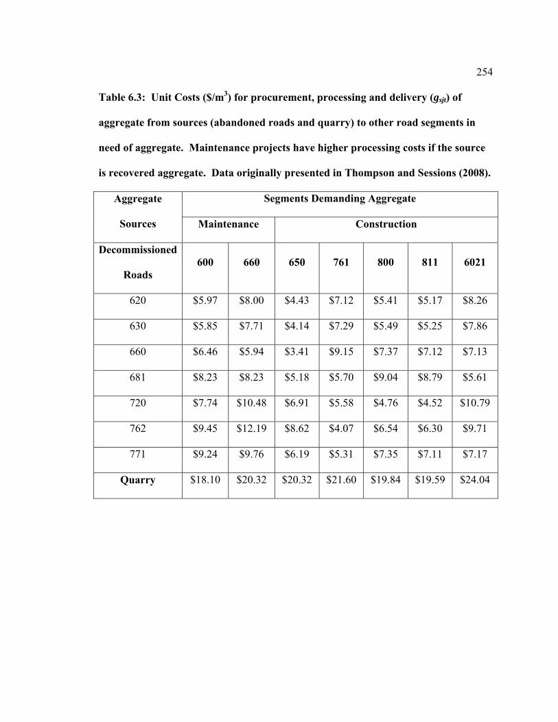
254 Table 6.3: Unit Costs ($/m3) for procurement, processing and delivery (gsjt) of
aggregate from sources (abandoned roads and quarry) to other road segments in
need of aggregate. Maintenance projects have higher processing costs if the source
is recovered aggregate. Data originally presented in Thompson and Sessions (2008).
Aggregate
Sources
Segments Demanding Aggregate
Maintenance Construction
Decommissioned
Roads 600 660 650 761 800 811 6021
620 $5.97 $8.00 $4.43 $7.12 $5.41 $5.17 $8.26
630 $5.85 $7.71 $4.14 $7.29 $5.49 $5.25 $7.86
660 $6.46 $5.94 $3.41 $9.15 $7.37 $7.12 $7.13
681 $8.23 $8.23 $5.18 $5.70 $9.04 $8.79 $5.61
720 $7.74 $10.48 $6.91 $5.58 $4.76 $4.52 $10.79
762 $9.45 $12.19 $8.62 $4.07 $6.54 $6.30 $9.71
771 $9.24 $9.76 $6.19 $5.31 $7.35 $7.11 $7.17
Quarry $18.10 $20.32 $20.32 $21.60 $19.84 $19.59 $24.04

255 Table 6.4: Road segment information passed into knowledge base to evaluate each
road segment’s relative effect on the aquatic environment. Columns, from left to
right, present information on number of stream crossing per kilometer, distance
from the road segment to a stream, and the road segment’s position on hillslope.
Road Segment Stream
Crossings
Distance to
Stream
Hillslope
Position Slope
620 0 / km > 100 m Ridge 0%
630 0 / km > 100 m Ridge 14%
660 0 / km > 100 m Ridge 1%
681 0 / km 71 m Ridge 0%
720 1.70 / km 50 m Streamside 6%
762 0 / km > 100 m Ridge 8%
771 0 / km > 100 m Ridge 1%

256 Table 6.5: Calculated truth values scores representing the degree of truth of the
assertion, “the road has a high potential for causing damage to the aquatic
environment.” These hazard scores were used to weight the length of each road to
arrive at a proxy for environmental performance, hazard-weighted length of roads
decommissioned.
Road
Segment
Potential Environmental Impact Truth
Value
Score
Stream Channel Integrity Erosion Risk
Stream
Crossings
Distance to
Stream
Hillslope
Position Slope
620 0.00 0.00 0.50 0.00 0.13
630 0.00 0.00 0.50 0.93 0.66
660 0.00 0.00 0.50 0.07 0.18
681 0.00 0.29 0.50 0.00 0.29
720 0.34 0.50 0.00 0.40 0.50
762 0.00 0.00 0.50 0.53 0.51
771 0.00 0.00 0.50 0.07 0.18

257 7 Conclusion
The purpose of this dissertation was to develop decision support models that will
lead to improved economic and environmental efficiency in the management of forest
road networks. In particular, I focused on developing methods to quantify the inherent
tradeoffs associated with forest road management and protection of aquatic resources. A
major contribution is the formulation and implementation of optimization approaches that
explicitly consider multiple objectives, in order to identify the tradeoff surface comprised
of efficient, or non-dominated, solutions. This, in turn, allows for an improved
understanding of the relationship between increased expenditures and the associated
marginal environmental benefits. It also allows for landowners to evaluate their current
practices and identify where improvements can be made. To the author’s knowledge this
dissertation constitutes the first application of technical efficiency to forest road erosion
control. Transitioning to a multi-objective planning paradigm is appropriate for forest
road management, where uncertainty exists with regard to identification of target
environmental performance levels, where objectives are quantitatively expressed in non-
commensurate scales, and where road management decisions necessarily involve
informed compromise.
My work reflects an interdisciplinary approach, integrating forest engineering
principles with a diverse array of other fields, including applied economics,
combinatorial optimization, multi-objective optimization, multi-criteria decision making,
graph and network theory, computer science, and evolutionary computation. Drawing
from these fields, I developed computer-based decision aids, which pair mathematical

258 formulations with appropriate solution methods. In Chapter 2, I introduced the notion of
technical efficiency and illustrated application of the concept to forest road erosion
control. The intent of the chapter was to demonstrate the utility of adopting an a
posteriori optimization approach, wherein the decision maker’s preferences are elicited
only after being presented with the realm of feasible and efficient possibilities. Though
methods exist to systematically elicit and weight preferences, a priori optimization
approaches suffer from the facts that preferences can change, and there generally is no
single answer that simultaneously optimizes all objectives. In subsequent chapters I
focus on application of technical efficiency to improve efficiency of specific road
management activities: regular maintenance (grading), and road removal and aggregate
resource management.
Another contribution of this dissertation is the extension of decision support
frameworks from single to multiple objective formulations. Chapters 3-4 illustrate this
extension for vehicle routing algorithms designed to intelligently deploy forest road
maintenance vehicles. Chapters 5-6 illustrate this extension for mixed-integer
formulations that identify optimal aggregate recycling and road removal policies.
Extending analyses to multi-objective frameworks requires the explicit definition of
metrics for environmental performance. Generating estimates of treatment efficacy is a
prerequisite for prioritizing treatments on the basis of cost/benefit, as well as for
evaluating how well environmental objectives are met as a result of treatment. In some
locales, generation of a predictive sediment inventory is also a regulatory requirement, as
I described in Chapter 1. For this dissertation I relied upon published, peer-reviewed

259 models that estimate sediment production and delivery (Chapter 2), estimate rut depth
formation in response to traffic (Chapter 4), and assign segment-level hazard, or risk,
scores (Chapter 6). I also considered an implicit benefit from treatment (Chapter 3) and
adopted a common policy among managers in the western U.S., to maximize the length
of roads treated (Chapter 5).
Lastly, this dissertation contributes to the discipline by advancing the notion that
aggregate recycling can effectively subsidize road decommissioning projects.
Procurement and delivery costs associated with recovering aggregate from
decommissioned roads can be significantly less than aggregate procured from quarries,
providing opportunities for substantial cost savings. On federal land, recognizing this
potential and planning appropriately could help managers improve and/or remove
additional roads given their limited budgets. Other state and private landowners more
concerned with timber production will be interested in improving the overall efficiency of
their aggregate management practices. As I demonstrate, aggregate recycling projects
have and continue to be implemented in practice, and my work facilitates these activities
by providing a framework for systematic analysis.
My work is immediately relevant and is intended to benefit both public and
private forest transportation managers. On public lands in the Pacific Northwest, where
watershed restoration is a dominant management objective, this research should facilitate
strategic road removal and improvement planning. Incorporating aggregate recycling
into current management practices, where practical, should release resources for other
restoration-oriented activities, ideally resulting in better achievement of the goals of the

260 Aquatic Conservation Strategy. Private landowners can adopt formulations
recommended here to improve their overall erosion control strategies, to improve grading
practices, and to reduce the overall cost of aggregate management. Identifying the
efficient frontier provides valuable information on what is and what is not possible with
respect to efficient management, and should help landowners better understand their
respective tradeoff curves, possibly to demonstrate that additional regulatory restrictions
are unnecessary or impractical.
Perhaps the greatest rationale for private landowners to adopt a multi-objective
planning paradigm is the specter of additional regulatory restrictions stemming from the
Clean Water Act. Already, road-related sediment is targeted as a contributing source of
pollution in many water quality limited streams subject to total maximum daily loads
(TMDLs), and regional water quality management plans, such as the General Waste
Discharge Requirement program administered by the California North Coast Regional
Water Quality Board, can place additional limitations on landowners. Perhaps most
worrisome to landowners, forest roads and their associated drainage structures may be
considered as “point sources” of pollution, and therefore subject to National Pollutant
Discharge Elimination System (NPDES) permitting requirements. District courts in
California and Oregon have reached conflicting decisions on this matter, with an appeal
currently before the 9th Circuit Court of Appeals. As outlined in Chapters 1-2, the
NPDES permitting process for conventional pollutants (including sediment) is entirely
premised upon tradeoff analysis. Forest landowners subject to permit requirements
would be forced to reduce road-related pollution up to the point where the marginal

261 benefits per dollar spent begin to markedly decline. Multi-objective programming
methods presented here are exactly the type of decision support system required in this
context.
The remainder of this conclusion is dedicated to summarizing the major findings
and implications of each chapter in the dissertation, and discussing future work.
As the intent of this dissertation was to illustrate the potential for multi-objective
optimization techniques to improve efficiency in the objective space, we did not focus on
the decision space. An interesting area of research, therefore, is the search for
commonalities between efficient solutions, perhaps through pattern analysis or a similar
technique. For instance, it might be that a similar subset of road treatments appears in
most non-dominated solutions. The identification of emergent patterns might facilitate
on the ground decision-making, a more intuitive process driven by experience and
informed by pattern analysis. When analyzing optimal grading policies, we may begin to
see certain road segments assigned significantly higher grading frequencies, and begin to
formulate simpler heuristics with respect to grading decisions, such as grade proximal
segments in clusters, or target only specific problematic road segments irrespective of
their distance from each other. We might likewise develop overarching strategies for
road erosion control treatments such as focusing on removing hydrologic road/stream
connections, or applying additional aggregate on roads serving high levels of traffic, etc.
It is my belief that moving to multi-objective planning frameworks is both
appropriate and preferable for contemporary forest road management moving forward. I
hope this work will stimulate additional research into tradeoff analysis, and ultimately

262 will lead to improved economic and environmental efficiency in the management of
forest transportation networks.
7.1 Forest Road Erosion Control Using Technical Efficiency (Chapter 2)
Chapter 2 presented a novel application of decision support applied to forest road
management, wherein I made use of the principles of forest and industrial engineering to
identify efficient road management alternatives. Specifically I proposed the use of multi-
objective programming techniques to identify the efficient frontier between sediment
reduction and management costs. In natural resources management, road management in
particular, incorporation of competing objectives is common and therefore having a tool
to facilitate tradeoff analysis should prove useful. Ultimately, the tradeoff-analysis
techniques promoted in this chapter should facilitate improved and efficient forest road
management.
Future research could seek to apply the methods presented here across a larger
ownership, or to include a broader scope of possible treatments. For instance, researchers
could include as decision variables maintenance regimes, traffic levels, seasonal road
closure, and reduced tire inflation. Also important to include in the tradeoff analysis are
the opportunity costs of such management actions. Toman et al. (2007) for example
demonstrated that the opportunity costs associated with restricting wet weather timber
haul and harvest could be up to 18% of total net revenue. Work pairing tradeoff analysis
with adaptive management paradigms would also be a promising direction. For instance,
it may be possible to incorporate model uncertainty into our multi-objective

263 programming approach, perhaps through robust optimization or other techniques.
Alternatively, it may be possible to develop approaches that identify not only optimal
allocations of resources between monitoring and treatment, but what types of monitoring
and treatment to apply.
Advancements in computing capacity and in algorithmic development
increasingly make solving more complex problems, such as those with multiple
objectives, possible. I therefore expect that techniques to identify efficient frontiers will
become preferable to traditional methods that seek to condense multiple objectives into a
single objective function. It is my hope that this manuscript demonstrating the utility of
technical efficiency for road management will spur future research into environmentally
and economically efficient multi-objective road management.
7.2 Intelligent Deployment of Forest Road Graders (Chapter 3)
Chapter 3 presented the design and application of a combinatorial heuristic to
route a forest road maintenance vehicle (grader) across a road network. The particular
solution method employed was tabu search paired with two local search routines, and
sought minimal cost tours, using tour length as a proxy. The local search routines sought
to increase overall tour efficiency by identifying instances where segments requiring
grading are traversed when en route to other segments requiring grading, and by
intelligently partitioning the tour if necessary due to exceeding the daily time limit. The
problem is modeled as an instance of the rural postman problem, where some subset of
edges in a network requires service. Other applications of the rural postman problem

264 include street sweeping and garbage collection. Road segments requiring grading were
identified according to a rubric based on road standard and road roughness index.
Initial testing on small road networks suggested the heuristic performed quite
well, reaching the known optimal solution in 2107 of 2400 runs (87.79%) for problem
instances with no operating constraints, and in 1037 of 1200 runs (86.42%) for instances
with operational time constraints. Aggregate percent deviation was 0.52% and 0.71%,
for the constraint-free scenario and operating time limit scenario, respectively. Even in
instances where the optimal solution was achieved only a relatively small proportion of
the time, the algorithm output the known 2nd best solution for a number of trials,
suggesting overall high performance.
For the much larger forest road network (modeled after a portion of the actual
road network of the McDonald Dunn Forest), the low average deviation suggests that the
heuristic consistently obtains good results, although there is no optimal solution as a basis
for comparison. Since it is difficult to compare solutions against a known or estimated
optimal value, it might be informative to learn if the heuristic would yield improvements
over current practices. To validate the model I developed a greedy heuristic, which might
mimic how a grader operator would traverse the network to grade the segments. Starting
from the depot, the grader first travels to the closest segment requiring grading and
services that segment. From there, the grader travels to the next nearest segment
requiring grading, and so on until all segments requiring grading have been serviced.
When tested on the largest network, the tabu search heuristic achieved a 12.5% reduction
in total grading time as compared to the greedy heuristic. Given that in practice an

265 operator may not know with certainty which is the nearest segment requiring service, it is
possible savings could be even higher. Further, given that in practice many grading
decisions are assigned not based on road condition but on time since the last grading, the
overall decision framework presented here may yield substantial reductions in overall
maintenance cost.
Future research should focus on both the solution methodology and the problem
definition. Improvements might be achievable by increasing the complexity of the tabu
search heuristic, such as utilizing a dynamic tabu list size or implementing harmonic
oscillation. The tour partition heuristic could also be expanded and possibly
implemented as a combinatorial heuristic such as tabu search or simulated annealing.
This method would be of great benefit in cases where the initial tour’s length is so great
as to require multiple partitions; the world of possible partitions increases exponentially
with respect to a unit increase in the number of partitions required. Incorporation of
time-windows would create a more realistic model, applicable perhaps to a high volume
network experiencing simultaneous haul and maintenance traffic. Some industrial
applications might involve a fleet of graders, operating from different depots or perhaps
without an assigned depot. Operational time constraints may not be quite so limiting,
allowing for a small exceedance in order to gain overall tour efficiency.
Future work could also be devoted to creating a broader decision framework for
determining which segments to grade. Rather than utilize a binary decision rule,
priorities could be established for segments requiring service. Thus the heuristic would
ensure that some segments of the highest priority are graded, but in addition would seek

266 opportunities to grade other high priority segments. If successfully implemented this
framework could free up future resources for other maintenance activities, hopefully
preventing future drainage and transportation problems. Perhaps this method would best
be employed in scenarios where the manager’s goal is to achieve the highest level of
maintenance possible, rather than a goal of cost minimization.
The intent of Chapter 3 is to demonstrate the potential for cost savings in grader
scheduling and deployment. My developed heuristic performed well on both cyclical and
dendritic networks, the latter being more common in mountainous terrain. Results
demonstrate the gains possible from using computational methods to evaluate complex
decisions, especially in light of the current management practices, which cannot or do not
account for the combinatorial nature of the networks. The tabu search heuristic presented
in this chapter can provide for improved decision making with regard to routing graders,
and could improve overall road maintenance.
7.3 Identifying Optimal Forest Road Grading Policies Using a Multi-Objective
Evolutionary Algorithm (Chapter 4)
Chapter 4 extended the work of chapter 3 to consider vehicle operating costs in
addition to maintenance costs, and to simultaneously seek to optimize an environmental
objective. The hazard-weighted rut depth for each road segment was identified as a
suitable proxy for environmental performance. Rut depth was selected because it is an
indicator of the degree to which the surface of the road is degraded, because higher rut
depths increase vehicle operating costs, because the presence of ruts can substantially

267 increase the risk of environmental degradation, and because the act of grading is designed
specifically to remove ruts and other surface failures (washboarding, potholes, etc.).
Hazard weights were assigned based upon segment length, recognizing the importance of
flow path length in sediment delivery.
Substantial sums are expended on gravel road maintenance throughout the world,
but there has been limited research directed towards systematically managing gravel
roads. Road maintenance and transport activities have been linked to sediment
production, but again, there has been limited research directed toward systematically
managing roads for sediment production. In the U.S., roads are receiving increasing
attention for their negative impacts on water quality, particularly relating to impacts on
fish. Although this attention has primarily been focused on forest lands, increasing
attention is being directed toward aggregate surfaced roads on non-forested lands as well.
I brought together the ideas for managing roads to simultaneously minimize user costs
and environmental degradation associated with formation of ruts and other road surface
failures. My examples have drawn coefficients from empirical results from the literature.
They are not intended to be handbook ready formulas, but are drawn from specific
studies and are intended to illustrate a conceptual system for approaching aggregate road
management.
Future work in this area could focus on improving development of both the
solution algorithm and the operational model. Though solutions did appear to span large
regions of the objective space, it may be fruitful to consider using the notion entropy to
promote diversity along the non-dominated front (Farhang-Mehr and Azarm 2002). One

268 option mentioned earlier is to move to a parallel processing setup to speed up fitness
evaluations, and possibly to include much larger populations to offer a wider look into
the decision space. As we emphasized the role of mutation, considering other MOEAs
that focus on mutation could also be interesting. The Pareto Archived Evolution Strategy
of Knowles and Corne (2000), for instance, abandons recombination and only uses
mutation to introduce diversity into the solution space.
On the operational model side, there exists the possibility to employ alternate
models forms for both economic and environmental objectives. Perhaps most promising
would be the adoption of alternate equations to model rut depth formation. A
formulation developed by the Army Corps of Engineers (Barber et al. 1978) and used by
the U.S. Forest Service for aggregate surface depth considers as input variables subgrade
strength, surface strength, tire pressure, and traffic. Using this approach would allow for
rut depth calculations more in line with what is expected for forest roads in the western
U.S. The model might also be expanded to incorporate log truck routing, or time
windows during which grading operations should not occur. Multiple maintenance
vehicles and multiple depots would be appropriate for larger networks.
My results demonstrate the utility of using a multi-objective approach; using the
Strength Pareto Evolutionary Algorithm I was able to identify efficient solutions that
dominated simulated management policies in terms of economic and environmental
performance. Adoption of an a posteriori optimization approach should facilitate tradeoff
analysis and lead to informed compromise. Ultimately this manuscript demonstrates that
use of computerized decision aids could lead to increased efficiency when determining

269 routes for graders to take over a road network. The multi-objective programming
techniques employed here should help landowners to “jointly produce” environmentally
benign, low-cost road networks. I hope this discussion will stimulate additional research
in road management of aggregate surfaced roads.
7.4 Optimal Policies for Aggregate Recycling from Decommissioned Forest Roads
(Chapter 5)
Chapter 5 presented a cost minimization model for aggregate recovery and reuse,
and demonstrated that use of such a model could result in substantial cost savings to
landowners, possibly freeing up resources to implement other restoration-oriented
projects. The chapter also presented a model to maximize environmental benefit from
road removal, using the total length of roads decommissioned as a proxy. Tested on an
example road network, incorporation of aggregate recycling demonstrates substantial
cost-savings relative to a baseline scenario without recycling, increasing the likelihood of
road decommissioning and reduced habitat degradation. I found that aggregate recycling
can result in up to 24% in cost savings (economic objective) and up to 890% in additional
length of roads decommissioned (environmental objective).
Use of these models with appropriate computer applications constitutes a decision
support aid that can be used to facilitate road removal decisions. These models are
general and easily extendable to other formulations, and should scale up to larger
planning problems readily given advancements in computing capacity and commercially
available solvers. While several simplifying assumptions were made for expository

270 purposes, the management models presented here have practical applications. Aggregate
recycling does occur in practice, as I demonstrated, and the formulation and data can be
adjusted accordingly for specific situations. Future research could incorporate a broader
road management optimization procedure, including additional removal treatments,
maintenance regimes, and the decision of when to remove a road. Further work could
also seek to apply an appropriate environmental hazard weighting techniques to
maximize the hazard-weighted kilometers of road decommissioned.
I believe this manuscript demonstrates the advantages of recycling aggregate,
which are both economic and environmental. Where feasible, transportation managers
should investigate opportunities to recover and reuse suitable aggregate, thereby
increasing efficiency while yielding environmental benefits. Using models such as those
presented here, it should be possible to identify which roads should be treated at a given
level and how aggregate sources should be allocated, in order to best achieve landowner
objectives.
7.5 Exploring Environmental and Economic Tradeoffs Associated with Aggregate
Recycling from Decommissioned Forest Roads (Chapter 6)
Chapter 6 extends the analysis from Chapter 5 in several significant ways. As
described above, the major change is the simultaneous consideration of both economic
and environmental objectives. That is, I seek to identify the entire frontier of efficient
solutions, not just the boundary (minimal cost, maximal benefit) solutions identified in
Chapter 5. Chapter 6 also extends the analysis of the role of aggregate recycling in

271 effectively subsidizing removal projects. I defined an accounting variable ES (effective
subsidy) as the difference in minimized cost between scenarios with and without the
opportunity to recycle aggregate, at a given level of environmental performance. I then
examined how ES varies with increasing levels of environmental performance. Results
suggest a synergistic relationship between this subsidy and environmental performance,
where subsidies generally increase with increasing environmental performance.
Transportation managers are therefore able to recover and reuse a non-renewable
resource, while at the same time promoting economic and environmental efficiency.
Chapter 6 also extends the work of Chapter 5 to include explicit calculation of a
hazard factor. In Chapter 5, the model assumes that all road segments slated for removal
are equally detrimental, and therefore the optimal treatment from an environmental
perspective is simply a function of length. This assumption is reasonable if it is also
assumed an experienced professional has identified appropriate levels of
decommissioning such that the expected future impacts per unit length from each
segment are nearly identical. With Chapter 6 to the contrary each segment is assigned a
score on the scale (0, 1) reflecting the degree to which the segment has potential to cause
environmental damage. Scores are assigned according to a model originally presented by
Girvetz and Shilling (2003), who analyzed the Tahoe National Forest road system for
potential environmental impacts according to the USDA Forest Service’s “Roads
Analysis” guidance document (USDA 1999).
This chapter presented mixed-integer, multi-objective mathematical programming
formulations to identify optimal aggregate recycling and road removal policies. Previous

272 research and real-world application have demonstrated the cost savings potential of
recovering and reusing aggregate from decommissioned forest roads. I extended
previous work by employing techniques to identify the efficient frontier of non-
dominated solutions, and to include hazard factors to differentially weight road segments
scheduled for removal. Identifying the frontier of non-dominated solutions facilitates
tradeoff analysis and the selection of compromise solutions. Decision makers whose
preferences are not best satisfied with boundary (minimal cost, maximal benefit)
solutions are able to explore other efficient possibilities.
The type of analysis presented here should ultimately facilitate watershed
restoration planning on federal lands in the Pacific Northwest. The utility of this approach
is not however limited to federal ownerships or to the specific region discussed here. My
proposed approach should help any class of landowners to manage their aggregate
resources. On private lands with high levels of timber harvest, landowners may now be
more likely to construct new temporary spurs with the intention of later recovering
aggregate. This may entail construction with geotextiles, which as I demonstrated may
increase cost savings.
My findings are not limited to the scenarios I modeled, where recovered
aggregate is to be used within the same planning period. The recovered aggregate tested
by Foltz and Truebe (2003), for instance, had been stockpiled for over 20 years.
Similarly, aggregate recovered from decommissioned forest roads on the Umpqua
National Forest was stockpiled for future use (Michael Karr, Work Supervisor, Road
Maintenance and Project Team, Umpqua National Forest, personal communication,

273 2007). Forward thinking managers may therefore opt to incur aggregate recovery costs
today in order to reduce aggregate procurements costs in the future.
Future work could seek to manage aggregate resources over a larger ownership,
or to incorporate additional decision variables such as aggregate stockpiling, road
improvement treatments, identification of which road segments to remove, and
identification of when to remove segments. Practitioners could also employ more
sophisticated and/or regionally-specific risk models. Here I intentionally adopted a
decision support system that is also used by federal agencies to prioritize watershed
restoration treatments and that has previously been used to prioritize road segments for
removal, but certainly other approaches are valid.
I hope this research stimulates additional interest into aggregate recycling, and
ultimately leads to improved economic and environmental efficiency in the management
of forest transportation networks.

274 7.6 References
Barber, V.C., Odom, E.C., and R.W. Patrick. 1978. The deterioration and reliability of pavements. Technical Report S-78-8. U.S. Army Engineers Waterways Experiment Station, Vicksburg, Miss.
Farhang-Merh, A., and S. Azarm. 2002. Diversity Assessment of Pareto Optimal Sets: An Entropy Approach. In: Proceedings of the 2002 Congress on Evolutionary Computation, Honolulu, HI, May, 2002.
Foltz, R., and M. Truebe. 2003. Locally Available Aggregate and Sediment Production. Transportation Research Record 1819, Paper No. LVR8-1050.
Girvetz, E. and Shilling, F. (2003), Decision Support for Road System Analysis and Modification on the Tahoe National Forest, Environmental Management, 32(2), 218-23.
Knowles, J.D., and D.W. Corne. 2000. Approximating the Nondominated Front Using the Pareto Archived Evolution Strategy. Evolutionary Computation 8(2): 149-172.
Toman, E.M., Skaugset, A.E., and G.E. Murphy. 2007. An Analysis of Opportunity Costs with Wet-Weather Timber Hauling. International Journal of Forest Engineering, 18(1), 17-23.
USDA Forest Service 1999. Roads analysis: informing decisions about managing the national forest transportation system. Misc. Rep. FS-643. Washington DC.

275 8 Bibliography
Akay, E.A., and J. Sessions. 2005. Applying the Decision Support System, TRACER, To Forest Road Design, Western Journal of Applied Forestry, 20(3): 184-191.
Allison, C., Sidle, R.C., and D. Tait. 2004. Application of Decision Analysis to Forest Road Deactivation in Unstable Terrain. Environmental Management 33(2): 173-185.
Amberg, A., Domschke, W., and S. Voß. 2000. Multiple Center Capacitated Arc Routing Problems: A Tabu Search Algorithm Using Capacitated Trees. European Journal of Operational Research 124(2): 360-376.
Anderson, A.E., Nelson, J.D., and R.G. D’Eon. 2006. Determining optimal road class and road deactivation strategies using dynamic programming. Canadian Journal of Forest Research 36(6): 1509-1518.
Aquatic and Riparian Effectiveness Monitoring Program. 2005. Watershed Monitoring for the Northwest Forest Plan: Data Summary Interpretation 2005, Oregon/Washington Coast Province. http://www.reo.gov/monitoring/watershed
Aruga, K., Chung, W., Akay, A., Sessions, J., and E.S. Miyata. 2007. Incorporating Soil Surface Erosion Prediction into Forest Road Alignment Optimization, International Journal of Forest Engineering, 18(1): 24-32.
Barber, V.C., Odom, E.C., and R.W. Patrick. 1978. The deterioration and reliability of pavements. Technical Report S-78-8. U.S. Army Engineers Waterways Experiment Station, Vicksburg, Miss.
Barrett, J.C., and W.J. Conroy. 2002. Improved Practices for Controlling both Point and Nonpoint Sources of Sediment Erosion from Industrial Forest Roads, paper presented at Total Maximum Daily Load (TMDL) Environmental Regulations, 2002 Conference, American Society of Agricultural and Biological Engineers, Fort Worth, TX, 11-13 March.
Battle, J.B., and M.I. Lipeles. 1998. Water Pollution, Anderson Publishing Company, OH.
Bettinger, P., Graetz, D., Boston, K., Sessions, J., and W. Chung. 2002. Eight heuristic planning techniques applied to three increasingly difficult wildlife-planning problems. Silva Fennica 36(2): 561-584.
Bettinger, P., Boston, K., and J. Sessions. 1999. Intensifying a heuristic forest harvest scheduling procedure with paired attribute decision choices. Canadian Journal of Forest Research 29: 1784-1792.
Bettinger, P., Sessions, J., and K.N. Johnson. 1998. Ensuring the Compatibility of Aquatic Habitat and Commodity Production Goals in Eastern Oregon with a Tabu Search Procedure, Forest Science, 44(1): 96-112.
Bettinger, P., Sessions, J., and K. Boston. 1997. Using tabu search to schedule timber harvests subject to spatial wildlife goals for big game. Ecological Modelling 94: 111-123.

276 Bilby, R.E., K. Sullivan, and S.H. Duncan. 1989. The generation and fate of road-surface
sediment in forested watersheds in southwestern Washington. Forest Science, 35(2): 453-468.
BLM 2003. The BLM Road Maintenance and Rock Wear Fees Calculation Handbook. Bolstad, C.E. and N.P. Peterson. 2005. Road Sediment Model: An Application for
Modeling Sediment from Forest Roads to Streams, paper presented at 28th Annual Meeting, Council on Forest Engineering, Fortuna, CA, 11-14 July.
Boston, K., Pyles, M., and A. Bord. 2008. Compaction of Forest Roads in Oregon – Room for Improvement. International Journal of Forest Engineering 19(1): 24-28.
Boston, K., and A. Bord. 2005. The Variability of Construction Practices and Material Properties Found on Forest Roads in Oregon, Proceedings of the 28th Council on Forest Engineering Conference, edited by P.J. Matzka, pp. 290-301, Council on Forest Engineering, Fortuna, CA.
Boston, K. and P. Bettinger. 2002. Combining tabu search and genetic algorithms heuristic techniques to solve spatial harvest scheduling problems. Forest Science 48(1): 35-46.
Boston, K., and P. Bettinger. 1999. An analysis of Monte Carlo integer programming, simulated annealing, and tabu search heuristics for solving spatial harvest scheduling problems. Forest Science. 45(2): 292-301.
Brooks, E.S., Boll, J., Elliot, W.J., and T. Dechert. 2006. Global Positioning System/GIS-Based Approach for Modeling Erosion from Large Road Networks. Journal of Hydrologic Engineering 11(5): 418-426.
Brown, C., and J. Sessions. 1999. Variable tire pressure for tropical forests? A synthesis of concepts and applications. Journal of Tropical Forest Science 11(2): 380-400.
Burroughs, E.R., Jr., and J.G. King. 1989. Reduction of soil erosion on forest roads, General Technical Report INT-264. US Department of Agriculture, Forest Service, Intermountain Research Station, Ogden, UT, 21 pp.
Calkin, D.E., C.A. Montgomery, N.H. Schumaker, S. Polasky, J.L. Arthur, and D.J. Nalle. 2002. Developing a production possibility set of wildlife persistence and timber harvest value. Canadian Journal of Forest Research, 32(8), 1329-1342.
Caterpillar Inc. 2002. Caterpillar Performance Handbook. Version 33. Caterpillar Inc., Peoria, Illinois, USA.
Chung, W., and J. Sessions. 2003. NETWORK 2000, A Program For Optimizing Large Fixed And Variable Cost Transportation Problems, Systems Analysis in Forest Resources, edited by G.J. Arthaud and T.M. Barrett, pp. 109-120. Kluwer Academic Publishers, Netherlands.
Coello Coello, C.A. 2006. Evolutionary Multi-Objective Optimization: A Historical View of the Field. IEEE Computational Intelligence Magazine 1(1) : 28-36.
Coello Coello, C.A. 1999. An Updated Survey of Evolutionary Multiobjective Optimization Techniques: State of the Art and Future Trends. In, Proceedings of the 1999 Congress on Evolutionary Computation. Piscataway, N.J., 1999, pp. 3-13.
277 Connaughton, K.P., and R.D. Fight. 1984. Applying Trade-Off Analysis to National
Forest Planning. Journal of Forestry, 82(11), 680-683. Contreras, M.A. and W. Chung. 2006. Using Ant Colony Optimization Metaheuristic in
Forest Transportation Planning, Proceedings of the 29th Annual Council on Forest Engineering Conference, edited by W. Chung and H.S. Han, pp. 221-232, Council on Forest Engineering, Coeur d’Alene, ID.
Corberán, A., Martí, R., and A. Romero. 2000. Heuristics for the Mixed Rural Postman Problem. Computers and Operations Research 27(2): 183-203.
Coulter, E.D., Sessions, J., and Wing, M.G. 2006. Scheduling Forest Road Maintenance Using the Analytic Hierarchy Process and Heuristics. Silva Fennica, 40(1), 143-160.
Dai, J.J., Lorenzato, S., and D.M. Rocke. 2004. A knowledge-based model of watershed assessment for sediment. Environmental Modelling and Software, 19(4), 423-433.
Damian, F. 2003. Cross-drain Placement to Reduce Sediment Delivery from Forest Roads to Streams. M.S. thesis, University of Washington, Seattle, WA.
de Steigeur, J.E., Liberti, L., Schuler, A., and B. Hansen. 2003. Multi-Criteria Decision Modelsfor Forestry and Natural Resources Management: An Annotated Bibliography. GTR NE-307. Newtown Square, PA: U.S. Department of Agriculture, Forest Service, Northeastern Research Station. 32 p.
Dorazio, R.M., and F.A. Johnson. 2003. Bayesian Inference and Decision Theory – A Framework for Decision Making in Natural Resource Management. Ecological Applications, 13(2), 556-563.
Ducheyne, E.I., De Wulf, R.R., and B. De Baets. 2006. A spatial approach to forest- management optimization: linking GIS and multiple objective genetic algorithms. International Journal of Geographical Information Science, 20(8), 917-928.
Ducheyne, E.I., De Wulf, R.R., and B. De Baets. 2004. Single versus multiple objective genetic algorithms for solving the even-flow forest management problem. Forest Ecology and Management 201(2-3): 259-273.
Eiselt, H.A., Gendreau, M., and G. Laporte. 1995a. Arc Routing Problems, Part I: The Chinese Postman Problem. Operations Research 43(2): 231-242.
Eiselt, H.A., Gendreau, M., and G. Laporte. 1995b. Arc Routing Problems, Part II: The Rural Postman Problem, Operations Research 43(3): 399-414.
Elliot, W.J., D.E. Hall, and S.R. Graves. 1999. Predicting sedimentation from forest roads. Journal of Forestry, 97(8), 23-29.
Elliot, W.J, and L.M. Tysdal. 1999. Understanding and reducing erosion from insloping roads. Journal of Forestry, 97(8), 30-34.
Environmental Protection Agency. 1999. Protocol for Developing Sediment TMDL’s. First Edition. October 1999.
Eschenbach, E.A., Teasley, R., Diaz, C., and M.A. Madej. 2005. Decision support for road decommissioning and restoration using genetic algorithms and dynamic programming. In: Redwood Science Symposium: What Does the Future Hold? USDA Forest Service General Technical Report PSW-GTR-194.

278 Faiz, A., and E. Staffini. 1979. Engineering economics of the maintenance of earth and
gravel roads. In, Proceedings of the Second International Conference on Low-Volume Roads, Transportation Research Record 702, TRB. P. 260-268.
Farhang-Merh, A., and S. Azarm. 2002. Diversity Assessment of Pareto Optimal Sets: An Entropy Approach. In: Proceedings of the 2002 Congress on Evolutionary Computation, Honolulu, HI, May, 2002.
Flanagan, S.A., M.J. Furniss, T.S. Ledwith, S. Thiesen, M. Love, K. Moore, and J. Ory. 1998. Methods for Inventory and Environmental Risk Assessment of Road Drainage Crossings. San Dimas, CA: USDA Forest Service Pacific Southwest Region. 45 p.
Foltz, R.B., and W.J. Elliot. 1998. Measuring and modeling impacts of tyre pressure on road erosion. In, Proceedings of the Seminar on Environmentally Sound Forest Roads and Wood Transport, Sinaia, Romania, FAO, Rome, pp. 205-214. http://www.fao.org/docrep/X0622E/X0622E00.htm
Foltz, R., and M. Truebe. 2003. Locally Available Aggregate and Sediment Production. Transportation Research Record 1819, Paper No. LVR8-1050.
Foltz, R., and E. Burroughs. 1991. A test of normal tire pressure and reduced tire pressures on forest roads: sedimentation effects. Pp. 103-112 in Proceedings, Forestry and Environmental Solutions. ASAE. New Orleans.
Forest Engineering Research Institute of Canada (FERIC). 2007. Opti-Grade. http://www.feric.ca/index.cfm?objectid=2DBAACB8-E081-222F-A48CDBA6DAA20324
Forman, R.T.T., and L.E. Alexander. 1998. Roads and their major ecological effects. Annual Review of Ecology and Systematics 29: 207-231
Furniss, M.J., Roelofs, T.D. and C.S. Yee. 1991. Road Construction and Maintenance. Influences of Forest and Rangeland Management on Salmonid Fishes and Their Habitats. American Fisheries Society Special Publication 19. Bethesda, MD. pp. 297-323.
Gallo, K., Lanigan, S.H., Eldred, P., Gordon, S.N., and C. Moyer. 2005. Northwest forest plan: the first 10 years (1994-2003). Preliminary assessment of the condition of watersheds. General technical report PNW-GTR-647. U.S. Department of Agriculture Forest Service, Pacific Northwest Research Station, Portland, Oregon.
GAO. 2001. Restoring Fish Passage Through Culverts on Forest Service and BLM Lands in Oregon and Washington Could Take Decades. GAO-02-136.
Gendreau, M., Hertz, A., and G. Laporte. 1994. A Tabu Search Heuristic for the Vehicle Routing Problem. Management Science 40(10): 1276-1290.
Girvetz, E. and Shilling, F. 2003. Decision Support for Road System Analysis and Modification on the Tahoe National Forest. Environmental Management 32(2): 218-23.
Glover, F., and G. Kochenberger. 2003. Handbook of Metaheuristics. Kluwer Publishers. 556 p.
Glover, F. 1989. Tabu Search – Part I. ORSA Journal of Computing 1(3): 190-206. Glover, F. 1990. Tabu Search – Part II. ORSA Journal of Computing 2(1): 4-32.

279 Gucinski H., Furniss M.J., Ziemer R.R., and M.H. Brookes. 2001. Forest roads: a
synthesis of scientific information. General Technical Report PNW-GTR-509. Portland, OR: US Department of Agriculture, Forest Service, Pacific Northwest Research Station.
Haimes, Y.Y., Lasdon, L.S., and D.A. Wismer. 1971. On a bicriterion formulation of the problems of integrated system identification and system optimization. IEEE Transactions on Systems, Man, and Cybernetics 1(3): 296-297.
Harr R.D. and R.A. Nichols. 1993. Stabilizing forest roads to help restore fish habitats: a northwest Washington example. Fisheries 18: 18–22.
Heller, D. 2002. A New Paradigm for Salmon and Watershed Restoration. In Proceedings of the 13th International Salmonid Enhancement Workshop: 16-19 September 2002, Hotel Westport, Westport, Co. Mayo, Ireland.
Hertz, A., Laporte, G., and M. Mittaz. 2000. A Tabu Search Heuristic for the Capacitated Arc Routing Problem. Operations Research 48(1): 129-135.
Hicks, B.J., J.D. Hall, P.A. Bisson, and J.R. Sedell. 1991. Responses of Salmonids to Habitat Changes. Ch. 14 in W. R. Meehan, ed., Influences of Forest and Rangeland Management on Salmonid Fishes and Their Habitats. American Fisheries Society Special Publication 19. Bethesda, MD. pp. 483-518.
Hide, H. 1975. Investigation of vehicle operating costs in Kenya. Low Volume Roads, Special Report 160, Transportation Research Board, National Research Council, National Academy of Sciences, Washington DC. P. 355-375.
Hwang, C.L., and Masud, A.S.M. 1979. Multiple Objective Decision Making – Methods and Applications. Springer Verlag, Berlin, Germany.
Ish, T., and D. Tomberlin (2005), Simulation of surface erosion on a logging road in the Jackson Demonstration State Forest, Proceedings of the redwood forest science symposium: What does the future hold, edited by Standiford, R.B. Giusti, G.A., Valachovic, Y., Zielinski, W.J., and M.J. Furniss, Gen. Tech. Report PSW-GTR-194, pp. 457-463, USDA Forest Service, Albany, CA.
Jones, J.A., Swanson, F.J., Wemple, B.C., and K.U. Snyder. 2000. Effects of roads on hydrology, geomorphology, and disturbance patches in stream networks. Conservation Biology 14(1): 76-85
Jozefowiez, N., Semet, F., and E. Talbi. 2008. Multi-objective vehicle routing problems. European Journal of Operational Research 189(2): 293-309.
Kangas, J., and A. Kangas. 2005. Multiple criteria decision support in forest management – the approach, methods applied, and experiences gained. Forest Ecology and Management 207(1-2): 133-143.
Karlsson, J., Rönnqvist, M., and M. Frisk. 2006. RoadOpt: A decision support system for road upgrading in forestry. Scandinavian Journal of Forest Research 21(7): 5-15.
Kennedy, M.C., Ford, D.E., Singleton, P., Finney, M., and J.K. Agee (2008), Informed multi-objective decision-making in environmental management using Pareto optimality, Journal of Applied Ecology, 45(1), 181-192.

280 Kirby, M. and R.J. Lowe. 1975. Optimal policies for transporting rock to low-volume
roads. Low volume roads, Special Report 160. Transportation Research Board, National Research Council, National Academy of Sciences, Washington, DC. pp. 296-301.
Knowles, J.D., and D.W. Corne. 2000. Approximating the Nondominated Front Using the Pareto Archived Evolution Strategy. Evolutionary Computation 8(2): 149-172.
Kolka, R.K., and M.F. Smidt. 2004. Effects of forest road amelioration techniques on soil bulk density, surface runoff, sediment transport, soil moisture and seedling growth. Forest Ecology and Management 202: 313-323
Laumanns, M., Thiele, L, and E. Zitzler. 2006. An efficient, adaptive parameter variation scheme for metaheuristics based on the epsilon-constraint method. European Journal of Operations Research 169: 932-942.
Luce, C.H., and T.A. Black. 1999. Sediment production from forest roads in western Oregon. Water Resources Research 35(8): 2561-2570.
Luce, C.H., and T.A. Black. 2001. Effects of traffic and ditch maintenance on forest road sediment production, Proceedings of the Seventh Federal Interagency Sedimentation Conference, V-67 - V-74, U.S. Inter-agency Committee on Water Resources, Subcommittee on Sedimentation, Washington, D.C.
Luce C.H., Rieman B.E., Dunham J.B., Clayton, J.L., King, J.G. and T.A. Black. 2001. Incorporating aquatic ecology into decisions on prioritization of road decommissioning. Water Resources Impact 3: 8–14.
Lugo, A.E., and H. Gucinski. 2000. Function, effects, and management of forest roads. Forest Ecology and Management 133: 249-262
Madej M.A. 2001. Erosion and sediment delivery following removal of forest roads. Earth Surface Processes and Landforms 26: 175–90.
Madej, M.A., E.A. Eschenbach, C. Diaz, R. Teasley, and K. Baker. 2006. Optimization strategies for sediment reduction practices on roads in steep, forested terrain. Earth Surface Processes and Landforms 31: 1643-1656.
Mendoza, G.A., and H. Martins. 2006. Multi-criteria decision analysis in natural resource management: A critical review of methods and new modeling paradigms. Forest Ecology and Management 230(1-3): 1-22.
Mills, K. 2006. Environmental Performance Measures for Forest Roads. Proceedings of the 29th Council on Forest Engineering Conference, edited by W. Chung and H.S. Han, pp. 291-300, Council on Forest Engineering, Coeur d’Alene, ID.
Moll, J., Copstead, R., and D.K. Johansen (1997), Traveled Way Surface Shape. USFS Technology and Development Program, Water –Road Interaction Technology Series Documents.
Morris, H. 1963. Applied hydraulics in engineering. Ronald Press, NY. 455p. Mostaghim, S., Teich, J., and A. Tyagi. 2002. Comparison of data structures for storing
Pareto-sets in MOEAs. In, Proceedigns of the 2002 Congress on Evolutionary Computation, Part of the 2002 IEEE World Congress on Computational Intelligence, Hawaii. Piscataway, NJ: IEEE Press, May 12-17, 2002.

281 Murphy, G.E. 1998. Allocation of stands and cutting patterns to logging crews using a
tabu search heuristic. International Journal of Forest Engineering 9(1): 31-37. Nalle, D.J., C.A. Montgomery, J.L. Arthur, S. Polasky, and N.H. Schumaker. 2004.
Modeling joint production of wildlife and timber, Journal of Environmental Economics and Management, 48(3), 997-1017.
Newcombe C.P. and D.D. MacDonald. 1991. Effects of suspended sediments on aquatic ecosystems. North American Journal of Fisheries Management 11(1): 72–82.
Nehlsen, W., Williams, J.E., and J.A. Lichatowich. 1991. Pacific Salmon at the Crossroads: Stocks at Risk from California, Oregon, Idaho and Washington. Fisheries 16(2): 4-21.
O’Hanley, J.R., and Tomberlin, D. 2005. Optimizing the removal of small fish passage barriers. Environmental Modeling and Assessment 10: 85-98.
Olsson, L. 2007. Optimal upgrading of forest road networks: Scenario analysis vs. stochastic modeling. Forest Policy and Economics 9(8): 1071-1078.
Olsson, L., and P. Lohmander. 2005. Optimal forest transportation with respect to road investments. Forest Policy and Economics 7(3): 369-379.
Olson, C.M. and B. Orr. 1999. Combining tree growth, fish and wildlife habitat, mass wasting, sedimentation, and hydrologic models in decision analysis and long-term forest planning. Forest Ecology and Management, 114(2-3), 339-348.
Oregon Department of Forestry. 2003. Wet Weather Road Use. Forest Practices Technical Note #9. http://egov.oregon.gov/ODF/PRIVATE_FORESTS/docs/fp/WetSeasonRoadUseFPTechNote9.pdf
Oregon Department of Forestry. 1998. Forest Road Sediment and Drainage Monitoring Project Report for Private and State Lands in Western Oregon. Monitoring Technical Report #10. http://egov.oregon.gov/ODF/PRIVATE_FORESTS/docs/fp/RoadSediment.pdf
Pearce, W. 1992. The MIT dictionary of modern economics. Cambridge: MIT Press. Pess, G.R., Beechie, T.J., Williams, J.E., Whitall, D.R., Lange, J.I., and J.R. Klochak.
2003. Watershed Assessment Techniques and the Success of Aquatic Restoration Activities. Chapter 8 in R.C. Wissmar and P.A. Bisson (eds.), Strategies for restoring river ecosystems: Sources of variability and uncertainty in natural and managed systems. American Fisheries Society, Bethesda, MD.
Provencher, Y. 1995. Optimizing Road Maintenance Intervals. Proceedings of the Sixth International Conference on Low-Volume Roads, Volume I, Minneapolis, MN, June 25-29, 1995. pp. 199-207.
Pyles, M. 2005. Monitoring: It is Our Job From Beginning to End, Proceedings of the 28th Council on Forest Engineering Conference, edited by P.J. Matzka, pp. 131-143, Council on Forest Engineering, Fortuna, CA.
Rackley, J. and W. Chung (2008), Incorporating Forest Road Erosion into Forest Resource Transportation Planning: A Case Study in the Mica Creek Watershed in Northern Idaho, Transactions of the ASABE, 51(1), 115-127.

282 Reeves, G.H., Williams, J.E., Burnett, K.M., and Gallo, K. 2006. The Aquatic
Conservation Strategy of the Northwest Forest Plan. Conservation Biology 20(2): 319-329.
Reid, L.M., and T. Dunne. 1984. Sediment Production from Forest Road Surfaces. Water Resources Research 20(11): 1753-1761.
Reynolds, K. M. 1999. EMDS users guide (version 2.0): knowledge-based decision support for ecological assessment. Gen. Tech. Rep. PNW-GTR-470. Portland, OR: U.S. Department of Agriculture, Forest Service, Pacific Northwest Research Station. 63 p.
Reynolds, K.M., Jensen, M., Andreasen, J., and Goodman, I. 2000. Knowledge-based assessment of watershed condition. Computers in electronics and agriculture 27: 315-333.
Reynolds, K.M. and S. Peets. 2001. Integrated Assessment and Priorities for Protection and Restoration of Watersheds. In Proceedings of IUFRO 4.11 Conference on Forest Biometry, Modeling and Information Science, 26-29 June 2001, Greenwich, UK, 2001.
Reynolds, K.M., and P.F. Hessburg. 2005. Decision support for integrated landscape evaluation and restoration planning. Forest Ecology and Management 207(1-2): 263-278.
Rice, R.M., and J. Lewis. 1991. Estimating Erosion Risks Associated With Logging and Forest Roads in Northwestern California, Water Resources Bulletin, 27(5), 809-818.
Richards, E. W., and E. A. Gunn. 2003. Tabu search design for difficult forest management optimization problems. Canadian Journal of Forest Research 33(6): 1126-1133.
Richards, E.W., and E.A. Gunn. 2000. A Model and Tabu Search Method to Optimize Stand Harvest and Road Construction Schedules. Forest Science 46(2): 188-203.
Roni, P., Beechie, T.J., Bilby, R.E., Leonetti, F.E., Pollock, M.M., and G.R. Pess. 2002. A Review of Stream Restoration Techniques and a Hierarchical Strategy for Prioritizing Restoration in Pacific Northwest Watersheds. North American Journal of Fisheries Management 22(1): 1-20.
Roper, B.B., Dose, J.J., and J.E. Williams. 1997. Stream Restoration: Is Fisheries Biology Enough? Fisheries 22(5): 6-11.
Rudolph. G. and A. Agapie. 2000. Convergence properties of some multi-objective evolutionary algorithms,” In Proceedings of the 2000 Conference on Evolutionary Computation, vol. 2, pp. 1010–1016, Piscataway, New Jersey, IEEE Press, July 2000.
Sadagopan, S., and A. Ravindran. 1982. Interactive solution of bi-criteria mathematical program. Naval Research Logistics Quarterly 29(3): 443-459.
Sample, V.A., Price, W., Donnay, J.S., and C.M. Mater. 2007. National Forest Certification Study. Pinchot Institute for Conservation. http://www.pinchot.org/current_projects/forest_cert/certification
Sessions J., Boston, K., Wing, M., Akay, A., Theisen, P., and R. Heinrich. 2007. Forest Roads Operations in the Tropics. Springer. 170p.

283 Sessions, J., Boston, K., Thoreson, R., and K. Mills. 2006. Optimal policies for
managing aggregate resources on temporary forest roads. Western Journal of Applied Forestry 21(4): 207-216.
Skaugset, A.E., Marbet, C.E., Gilbert, E.H., and K.S. Ellington (2007), The Hydrology of Forest Roads in the Central Oregon Coast Range, Watershed Management to Meet Water Quality Standards and TMDLs, edited by A. McFarland and A. Saleh, pp. 598-604, ASABE, San Antonio, TX.
Stückelberger, J.A., Heinimann, H.R., Chung, W., and M. Ulber (2006), Automatic road- network planning for multiple objectives. Proceedings of the 29th Council on Forest Engineering Conference, edited by W. Chung and H.S. Han, pp. 233-248, Council on Forest Engineering, Coeur d’Alene, ID.
Surfleet, C. 2008. Uncertainty in forest road hydrologic modeling and catchment scale assessment of forest road sediment yield. PhD dissertation, Oregon State University, Corvallis, OR
Switalski, T.A., Bissonette, J.A., DeLuca, T.H., and M.A. Madej. 2004. Benefits and impacts of road removal. Frontiers in Ecology and the Environment 2(1): 21-28.
Tan, K.C., Lee, T.H., and E.F. Khor. 2002. Evolutionary Algorithms for Multi- Objective Optimization: Performance Assessments and Comparisons. Artificial Intelligence Review 17(4): 253-290.
Thompson, M., and D. Tomberlin. 2005. Erosion Control on Logging Roads. Institute for Operations Research and Management Sciences (INFORMS) 2005 Annual Meeting: Ecologies, Economies and Operations Research, San Francisco, CA.
Thompson, M., Boston, K., Arthur, J., and J. Sessions. 2007. Intelligent Deployment of Forest Road Graders, International Journal of Forest Engineering, 18(2), 15-23.
Thompson, M. and J. Sessions. 2008. Optimal Policies for Aggregate Recycling from Decommissioned Forest Roads, Environmental Management, 42(2), 297-309.
Toman, E.M., Skaugset, A.E., and G.E. Murphy. 2007. An Analysis of Opportunity Costs with Wet-Weather Timber Hauling. International Journal of Forest Engineering, 18(1), 17-23.
Tomberlin, D., Baxter, W.T., Ziemer, R.R., and M. Thompson. 2002. Logging roads and aquatic habitat protection in the California redwoods. Poster. 2002 SAF National Convention, 5-9 October 2002, Winston-Salem, NC. http://www.fs.fed.us/psw/rsl/projects/water/Tomberlin.pdf
Toth, S.F., M.E. McDill, and S. Rebain. 2006. Finding the Efficient Frontier of a Bi- Criteria, Spatially Explicit, Harvest Scheduling Model, Forest Science, 52(1), 93-107.
Toth, S.F. and M.E. McDill. 2008. Promoting Large, Compact Mature Forest Patches in Harvest Scheduling Models, Environmental Modeling and Assessment, 13(1), 1-15.
Trombulak, S.C. and C.A. Frissell. 2000. Review of ecological effects of roads on terrestrial and aquatic communities. Conservation Biology 14(1): 18–30.

284 USDA and USDI. 1994. Record of Decision for amendments to Forest Service and
Bureau of Land Management Planning documents within the range of the northern spotted owl and standards and guidelines for management of habitat for late-successional and old-growth forest related species within the range of the northern spotted owl. Portland, OR.
USDA Forest Service 1999. Roads analysis: informing decisions about managing the national forest transportation system. Misc. Rep. FS-643. Washington DC.
USDA Forest Service, 2001. Road Management Policy Website. http://www.fs.fed.us/eng/road_mgt/policy.shtml
USDA Forest Service, 2002. Road Management Website. http://www.fs.fed.us/eng/road_mgt/overview.shtml
Van Veldhuizen, D.A., and G.B. Lamont. 2000. Multiobjective Evolutionary Algorithms: Analyzing the State-of-the-Art. Evolutionary Computation 8(2): 125-147.
Weaver, W. and D. Hagans. 2009. Road upgrading, decommissioning and maintenance – estimating costs on small and large scales. http://www.st.nmfs.gov/st5/Salmon_Workshop/10_Weaver_and_Hagans.pdf
Weaver, W., and D. Hagans. 1999. Storm-Proofing Forest Roads. In: Proceedings of the International Mountain Logging and 10th Pacific Northwest Skyline Symposium, Oregon State University Department of Forest Engineering and International Union of Forestry Research Organizations, Corvallis, OR. March 28-April 1, 1999. Pp. 230-245.
Wolpert, D.H., and W.G. Macready. 1997. No Free Lunch Theorems for Optimization. IEEE Transactions on Evolutionary Computation 1(1): 67-82.
Zitzler, E., Laumanns, M., and L. Thiele. 2001. SPEA2: Improving the Strength Pareto Evolutionary Algorithm. In K. Giannakoglou et al., editor, EUROGEN 2001. Evolutionary Methods for Design, Optimization and Control with Applications to Industrial Problems, pp. 95–100, Athens, Greece, 2002.
Zitzler E, Laumanns M, Thiele L. SPEA2: improving the strength Pareto evolutionary algorithm. Tech Rep TIK-103, Department of Electrical Engineering, Swiss Federal Institute of Technology, 2001.
Zitzler, E., K. Deb, and L. Thiele. 2000. Comparison of Multiobjective Evolutionary Algorithms: Empirical Results. Evolutionary Computation 8(2): 173-195.
Zitzler, E., and L. Thiele. 1999. Multiobjective Evolutionary Algorithms: A Comparative Case Study and the Strength Pareto Approach. IEEE Transactions on Evolutionary Computation 3(4): 257-271.