amortization - depreciation and depletionbalasubramanian.yolasite.com/resources/solved examples...
TRANSCRIPT
Amortization - Depreciation and Depletion
Amortization describes the equivalence of a capital sum over a period of time. In process
industries, it may be considered as a program or policy whereby the owners (stock-holders) of the
company have their investment on depreciable capital that is partly protected against loss.
An analysis of costs and profits for any business operation requires recognition of the fact that physical
assets decrease in value with age. This decrease in value may be due to physical deterioration,
technological advances, economic changes, or other factors, which ultimately will cause retirement of
the property. The reduction in value due to any of these causes is a measure of the depreciation. The
economic function of depreciation, therefore, can be employed as a means of distributing the original
expense for a physical asset over the period during which the asset is in use. Because the engineer
thinks of depreciation as a measure of the decrease in value of property with time, depreciation can
immediately be considered from a cost viewpoint.
For example, suppose a piece of equipment had been put into use 10 years ago at a total cost of
$31,000. The equipment is now worn out and is worth only $1000 as scrap material. The decrease in
value during the lo-year period is $30,000; however, the engineer recognizes that this $30,000 is in
reality a cost incurred for the use of the equipment. This depreciation cost was spread over a period of
10 years, and sound economic procedure would require part of this cost to be charged during each of
the years. The application of depreciation in engineering design, accounting, and tax studies is almost
always based on costs prorated throughout the life of the property.
According to the United States, Internal Revenue Service, depreciation is defined as “A
reasonable allowance for the exhaustion, wear, and tear of property used in the trade or business
including a reasonable allowance for obsolescence.” The terms amortization and depreciation are
often used interchangeably. Amortization is usually associated with a definite period of cost
distribution, while depreciation usually deals with an unknown or estimated period over which the
asset costs are distributed. Depreciation and amortization are of particular significance as an
accounting concept that serves to reduce taxes.
Depreciation
Depreciation has many meanings, but only two are discussed in our syllabus
1. loss of value of capital with the time when equipment wears out or becomes obsolete.
2. the systematic allocation of costs of an asset that produces an income from operations.
In short, depreciation may be considered as a cost for protection of depreciating capital without interest
over a period, which the capital (asset or equipment) is used.
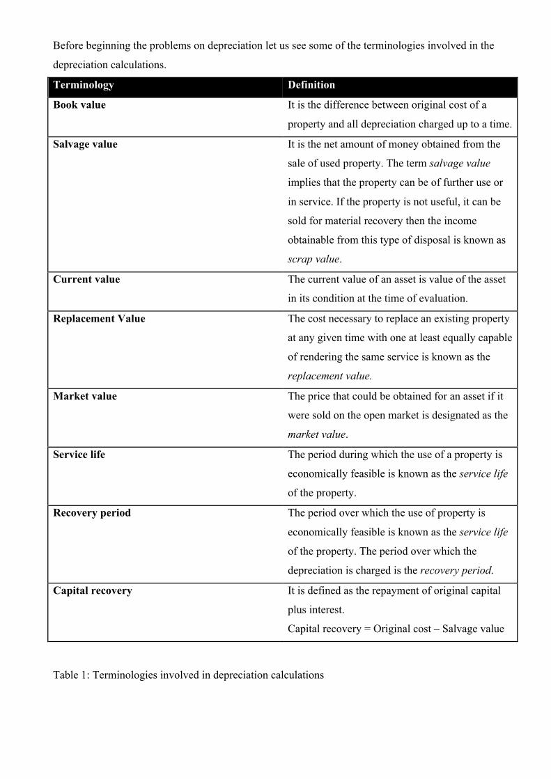
Before beginning the problems on depreciation let us see some of the terminologies involved in the
depreciation calculations.
Terminology Definition
Book value It is the difference between original cost of a
property and all depreciation charged up to a time.
Salvage value
It is the net amount of money obtained from the
sale of used property. The term salvage value
implies that the property can be of further use or
in service. If the property is not useful, it can be
sold for material recovery then the income
obtainable from this type of disposal is known as
scrap value.
Current value The current value of an asset is value of the asset
in its condition at the time of evaluation.
Replacement Value The cost necessary to replace an existing property
at any given time with one at least equally capable
of rendering the same service is known as the
replacement value.
Market value The price that could be obtained for an asset if it
were sold on the open market is designated as the
market value.
Service life The period during which the use of a property is
economically feasible is known as the service life
of the property.
Recovery period The period over which the use of property is
economically feasible is known as the service life
of the property. The period over which the
depreciation is charged is the recovery period.
Capital recovery It is defined as the repayment of original capital
plus interest.
Capital recovery = Original cost – Salvage value
Table 1: Terminologies involved in depreciation calculations
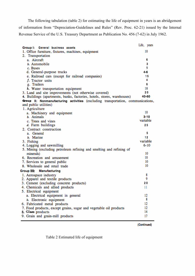
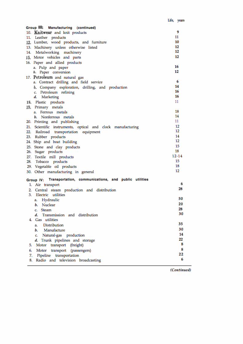
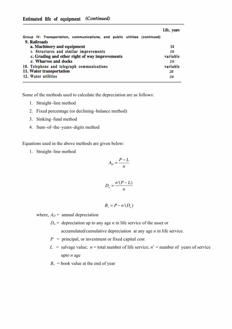
The following tabulation (table 2) for estimating the life of equipment in years is an abridgement
of information from “Depreciation-Guidelines and Rules” (Rev. Proc. 62-21) issued by the Internal
Revenue Service of the U.S. Treasury Department as Publication No. 456 (7-62) in July 1962.
Table 2 Estimated life of equipment
Some of the methods used to calculate the depreciation are as follows:
1. Straight–line method
2. Fixed percentage (or declining–balance method)
3. Sinking–fund method
4. Sum–of–the–years–digits method
Equations used in the above methods are given below:
1. Straight–line method
AD = P ! Ln
Dn =n '(P ! L)
n
Bv = P ! n '(Dn )
where, AD = annual depreciation
Dn = depreciation up to any age n in life service of the asset or
accumulated/cumulative depreciation at any age n in life service.
P = principal, or investment or fixed capital cost
L = salvage value; n = total number of life service; n’ = number of years of service
upto n age
Bv = book value at the end of year
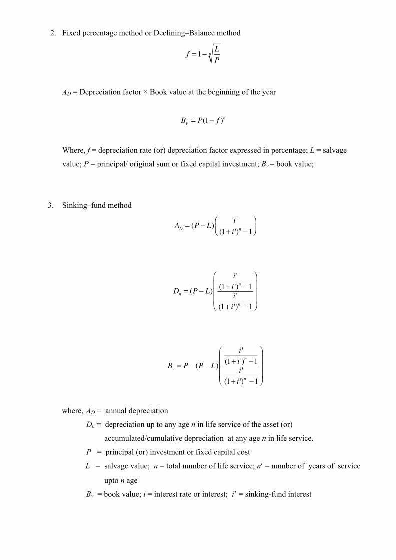
2. Fixed percentage method or Declining–Balance method
f =1! LP
n
AD = Depreciation factor × Book value at the beginning of the year
BV = P(1! f )n
Where, f = depreciation rate (or) depreciation factor expressed in percentage; L = salvage
value; P = principal/ original sum or fixed capital investment; Bv = book value;
3. Sinking–fund method
AD = (P ! L) i '(1+ i ')n !1
"#$
%&'
Dn = (P ! L)
i '(1+ i ')n !1
i '(1+ i ')n ' !1
"
#
$$$
%
&
'''
Bv = P ! (P ! L)
i '(1+ i ')n !1
i '(1+ i ')n ' !1
"
#
$$$
%
&
'''
where, AD = annual depreciation
Dn = depreciation up to any age n in life service of the asset (or)
accumulated/cumulative depreciation at any age n in life service.
P = principal (or) investment or fixed capital cost
L = salvage value; n = total number of life service; n’ = number of years of service
upto n age
Bv = book value; i = interest rate or interest; i’ = sinking-fund interest
4. Sum–of–the–years–digits method
Dn = (P ! L)" (Depreciation factor)Bv = (P !Dn )
Problem No. 1
If a heat exchanger costs $1,100 with 10 years of service life had a salvage value of $100. Estimate the
annual depreciation of heat exchanger using the following methods
(1) Straight–line method
(2) Fixed percentage (or) Declining–Balance method
(3) Sinking–fund method
(4) Sum-of-the-years–digits method.
Solution:
Given:
Principal (or) Original sum (or) Initial Investment (or) Fixed capital cost = $1,100
Service life of the heat exchanger = 10 years
Salvage value of the heat exchanger at the end of 10th year is = $100
Required:
Annual depreciation by
(1) Straight–line method
(2) Fixed percentage (or) Declining–Balance Method
(3) Sinking–fund method
(4) Sum–of–the–years–digits method and show the behavior of book value and
depreciation in graph for each of the above mentioned methods.
Calculation:
(1) Straight–line method
The annual depreciation (AD), depreciation up to any age n in life service
of the asset (Dn), and book value (Bv) at the end of each year from 0 to 10 is calculated and
tabulated in table 1 as follows,
where, Bv = book value at the end of year
Dn = depreciation up to any age n in life service of the asset or
accumulated/cumulative depreciation at any age n in life service.
Bv = P ! n '(Dn )
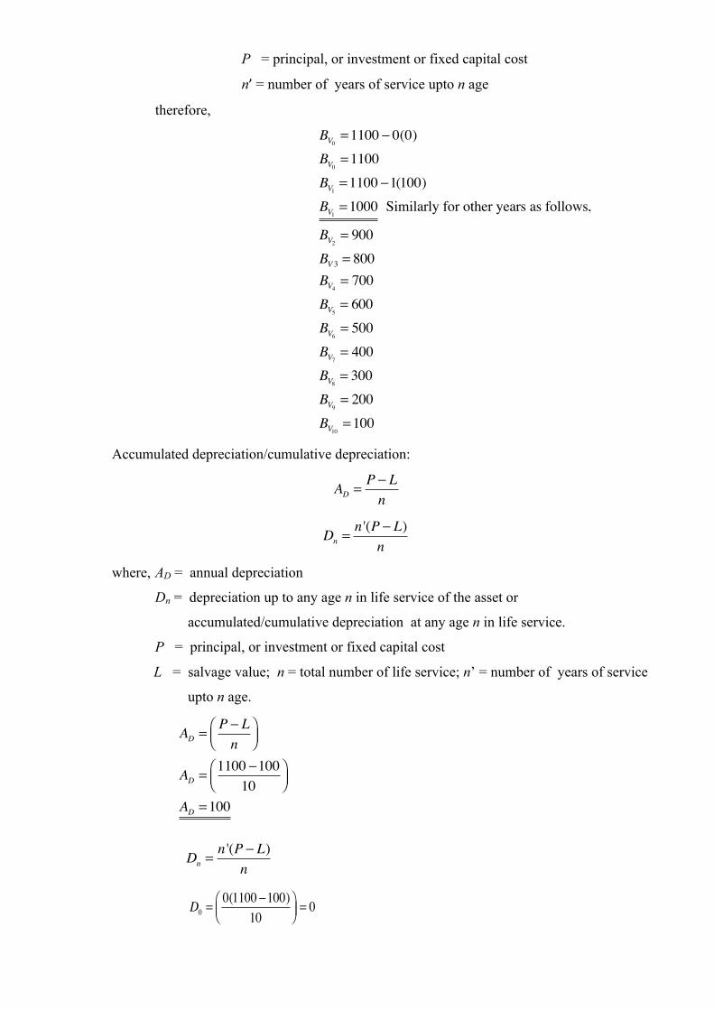
P = principal, or investment or fixed capital cost
n’ = number of years of service upto n age
therefore,
BV0=1100 ! 0(0)
BV0=1100
BV1=1100 !1(100)
BV1=1000 Similarly for other years as follows,
BV2= 900
BV 3 = 800BV4
= 700BV5
= 600BV6
= 500BV7
= 400BV8
= 300BV9
= 200BV10
=100
Accumulated depreciation/cumulative depreciation:
where, AD = annual depreciation
Dn = depreciation up to any age n in life service of the asset or
accumulated/cumulative depreciation at any age n in life service.
P = principal, or investment or fixed capital cost
L = salvage value; n = total number of life service; n’ = number of years of service
upto n age.
AD = P ! Ln
Dn =n '(P ! L)
n
Dn =n '(P ! L)
n
AD = P ! Ln
"#$
%&'
AD = 1100 !10010
"#$
%&'
AD =100
D0 =0(1100 !100)
10"#$
%&' = 0
D1 =1(1100 !100)
10"#$
%&' =100
D2 =2(1100 !100)
10"#$
%&' = 200
D3 =3(1100 !100)
10"#$
%&' = 300
D4 =4(1100 !100)
10"#$
%&' = 400
D5 =5(1100 !100)
10"#$
%&' = 500
D6 =6(1100 !100)
10"#$
%&' = 600
D7 =7(1100 !100)
10"#$
%&' = 700
D8 =8(1100 !100)
10"#$
%&' = 800
D9 =9(1100 !100)
10"#$
%&' = 900
D10 =0(1100 !100)
10"#$
%&' =1000
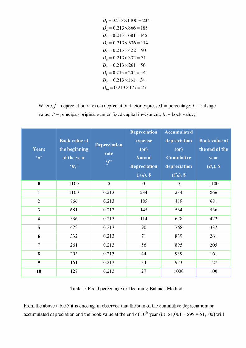
Thus, the calculations were carried out and the results are tabulated in table 3. To understand the
behavior of book vale and depreciation (depreciation up to any age n in life service of the asset or
accumulated/cumulative depreciation at any age n in life service) a graph is plotted and shown in
figure 1.
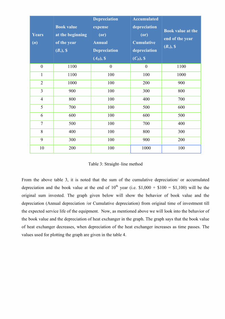
Years
(n)
Book value
at the beginning
of the year
(Bv), $
Depreciation
expense
(or)
Annual
Depreciation
(AD), $
Accumulated
depreciation
(or)
Cumulative
depreciation
(CD), $
Book value at the
end of the year
(Bv), $
0 1100 0 0 1100
1 1100 100 100 1000
2 1000 100 200 900
3 900 100 300 800
4 800 100 400 700
5 700 100 500 600
6 600 100 600 500
7 500 100 700 400
8 400 100 800 300
9 300 100 900 200
10 200 100 1000 100
Table 3: Straight–line method
From the above table 3, it is noted that the sum of the cumulative depreciation/ or accumulated
depreciation and the book value at the end of 10th year (i.e. $1,000 + $100 = $1,100) will be the
original sum invested. The graph given below will show the behavior of book value and the
depreciation (Annual depreciation /or Cumulative depreciation) from original time of investment till
the expected service life of the equipment. Now, as mentioned above we will look into the behavior of
the book value and the depreciation of heat exchanger in the graph. The graph says that the book value
of heat exchanger decreases, when depreciation of the heat exchanger increases as time passes. The
values used for plotting the graph are given in the table 4.
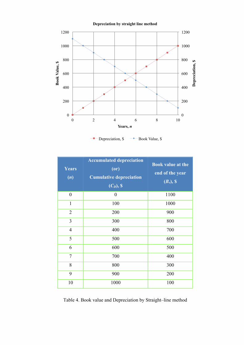
Years
(n)
Accumulated depreciation
(or)
Cumulative depreciation
(CD), $
Book value at the
end of the year
(Bv), $
0 0 1100
1 100 1000
2 200 900
3 300 800
4 400 700
5 500 600
6 600 500
7 700 400
8 800 300
9 900 200
10 1000 100
Table 4. Book value and Depreciation by Straight–line method
0
200
400
600
800
1000
1200
0
200
400
600
800
1000
1200
0 2 4 6 8 10
Dep
reci
atio
n, $
Boo
k Va
lue,
$
Years, n
Depreciation by straight line method
Depreciation, $ Book Value, $
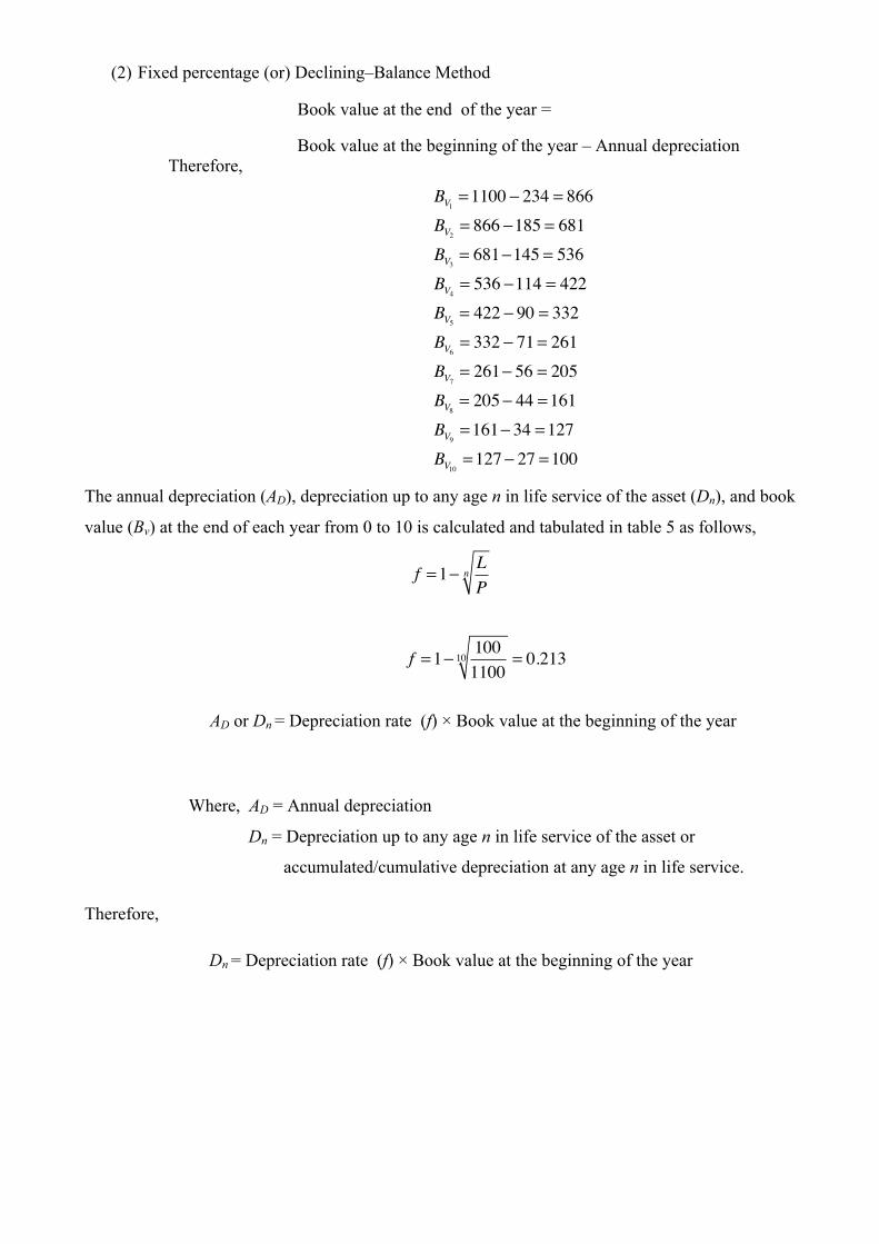
(2) Fixed percentage (or) Declining–Balance Method
Book value at the end of the year =
Book value at the beginning of the year – Annual depreciation
Therefore,
BV1 =1100 ! 234 = 866BV2 = 866 !185 = 681BV3 = 681!145 = 536BV4 = 536 !114 = 422BV5 = 422 ! 90 = 332BV6 = 332 ! 71= 261BV7 = 261! 56 = 205BV8 = 205! 44 =161BV9 =161! 34 =127BV10 =127! 27 =100
The annual depreciation (AD), depreciation up to any age n in life service of the asset (Dn), and book
value (Bv) at the end of each year from 0 to 10 is calculated and tabulated in table 5 as follows,
f =1! 1001100
10 = 0.213
AD or Dn = Depreciation rate (f) × Book value at the beginning of the year
Where, AD = Annual depreciation
Dn = Depreciation up to any age n in life service of the asset or
accumulated/cumulative depreciation at any age n in life service.
Therefore,
Dn = Depreciation rate (f) × Book value at the beginning of the year
f =1! LP
n
D1 = 0.213!1100 = 234D2 = 0.213!866 =185D3 = 0.213! 681=145D4 = 0.213! 536 =114D5 = 0.213! 422 = 90D6 = 0.213! 332 = 71D7 = 0.213! 261= 56D8 = 0.213! 205 = 44D9 = 0.213!161= 34D10 = 0.213!127 = 27
Where, f = depreciation rate (or) depreciation factor expressed in percentage; L = salvage
value; P = principal/ original sum or fixed capital investment; Bv = book value;
Years
‘n’
Book value at
the beginning
of the year
‘Bv’
Depreciation
rate
‘f ’
Depreciation
expense
(or)
Annual
Depreciation
(AD), $
Accumulated
depreciation
(or)
Cumulative
depreciation
(CD), $
Book value at
the end of the
year
(Bv), $
0 1100 0 0 0 1100
1 1100 0.213 234 234 866
2 866 0.213 185 419 681
3 681 0.213 145 564 536
4 536 0.213 114 678 422
5 422 0.213 90 768 332
6 332 0.213 71 839 261
7 261 0.213 56 895 205
8 205 0.213 44 939 161
9 161 0.213 34 973 127
10 127 0.213 27 1000 100
Table: 5 Fixed percentage or Declining-Balance Method
From the above table 5 it is once again observed that the sum of the cumulative depreciation/ or
accumulated depreciation and the book value at the end of 10th year (i.e. $1,001 + $99 = $1,100) will
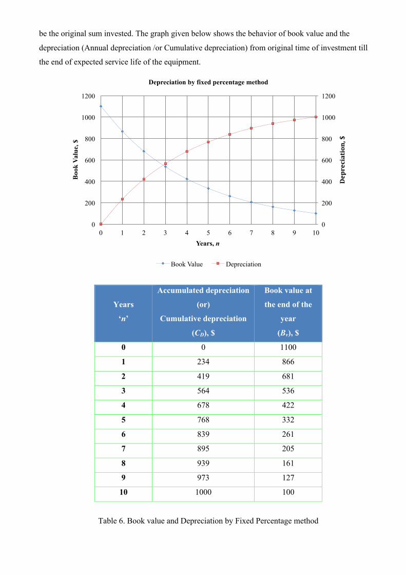
be the original sum invested. The graph given below shows the behavior of book value and the
depreciation (Annual depreciation /or Cumulative depreciation) from original time of investment till
the end of expected service life of the equipment.
Years
‘n’
Accumulated depreciation
(or)
Cumulative depreciation
(CD), $
Book value at
the end of the
year
(Bv), $
0 0 1100
1 234 866
2 419 681
3 564 536
4 678 422
5 768 332
6 839 261
7 895 205
8 939 161
9 973 127
10 1000 100
Table 6. Book value and Depreciation by Fixed Percentage method
0
200
400
600
800
1000
1200
0
200
400
600
800
1000
1200
0 1 2 3 4 5 6 7 8 9 10
Depreciation, $
Boo
k Va
lue,
$
Years, n
Depreciation by fixed percentage method
Book Value Depreciation
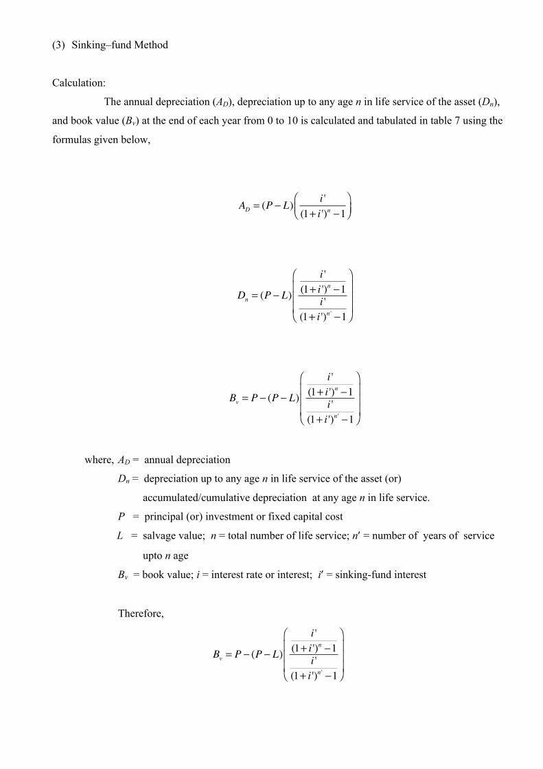
(3) Sinking–fund Method
Calculation:
The annual depreciation (AD), depreciation up to any age n in life service of the asset (Dn),
and book value (Bv) at the end of each year from 0 to 10 is calculated and tabulated in table 7 using the
formulas given below,
where, AD = annual depreciation
Dn = depreciation up to any age n in life service of the asset (or)
accumulated/cumulative depreciation at any age n in life service.
P = principal (or) investment or fixed capital cost
L = salvage value; n = total number of life service; n’ = number of years of service
upto n age
Bv = book value; i = interest rate or interest; i’ = sinking-fund interest
Therefore,
AD = (P ! L) i '(1+ i ')n !1
"#$
%&'
Dn = (P ! L)
i '(1+ i ')n !1
i '(1+ i ')n ' !1
"
#
$$$
%
&
'''
Bv = P ! (P ! L)
i '(1+ i ')n !1
i '(1+ i ')n ' !1
"
#
$$$
%
&
'''
Bv = P ! (P ! L)
i '(1+ i ')n !1
i '(1+ i ')n ' !1
"
#
$$$
%
&
'''
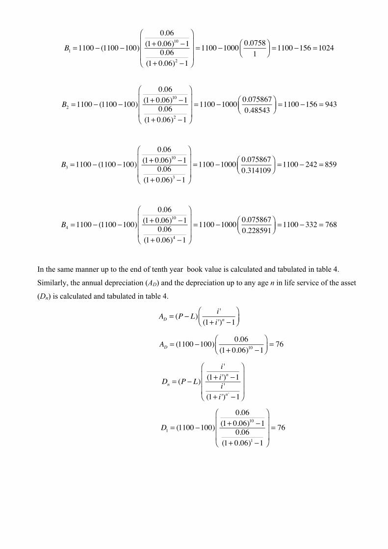
B1 =1100 ! (1100 !100)
0.06(1+ 0.06)10 !1
0.06(1+ 0.06)2 !1
"
#
$$$
%
&
'''=1100 !1000 0.0758
1"#$
%&' =1100 !156 =1024
B2 =1100 ! (1100 !100)
0.06(1+ 0.06)10 !1
0.06(1+ 0.06)2 !1
"
#
$$$
%
&
'''=1100 !1000 0.075867
0.48543"#$
%&' =1100 !156 = 943
B3 =1100 ! (1100 !100)
0.06(1+ 0.06)10 !1
0.06(1+ 0.06)3 !1
"
#
$$$
%
&
'''=1100 !1000 0.075867
0.314109"#$
%&' =1100 ! 242 = 859
B4 =1100 ! (1100 !100)
0.06(1+ 0.06)10 !1
0.06(1+ 0.06)4 !1
"
#
$$$
%
&
'''=1100 !1000 0.075867
0.228591"#$
%&' =1100 ! 332 = 768
In the same manner up to the end of tenth year book value is calculated and tabulated in table 4.
Similarly, the annual depreciation (AD) and the depreciation up to any age n in life service of the asset
(Dn) is calculated and tabulated in table 4.
AD = (1100 !100) 0.06(1+ 0.06)10 !1
"#$
%&'= 76
D1 = (1100 !100)
0.06(1+ 0.06)10 !1
0.06(1+ 0.06)1 !1
"
#
$$$
%
&
'''= 76
AD = (P ! L) i '(1+ i ')n !1
"#$
%&'
Dn = (P ! L)
i '(1+ i ')n !1
i '(1+ i ')n ' !1
"
#
$$$
%
&
'''
Years
‘n’
Book value at
the beginning
of the year
‘Bv’
Interest rate
‘ i’ ’
Depreciation
expense
(or)
Annual
Depreciation
(AD), $
Accumulated
depreciation
(or)
Cumulative
depreciation
(CD), $
Book value at
the end of the
year
(Bv), $
0 1100 0.06 0 0 1100
1 1100 0.06 76 76 1024
2 1024 0.06 76 156 943
3 943 0.06 76 242 859
4 859 0.06 76 332 768
5 768 0.06 76 428 673
6 673 0.06 76 529 571
7 571 0.06 76 637 463
8 463 0.06 76 751 349
9 349 0.06 76 872 228
10 228 0.06 76 1000 100
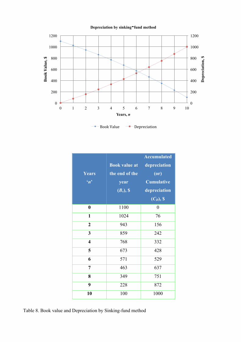
Table 7: Book value and depreciation by sinking–fund method
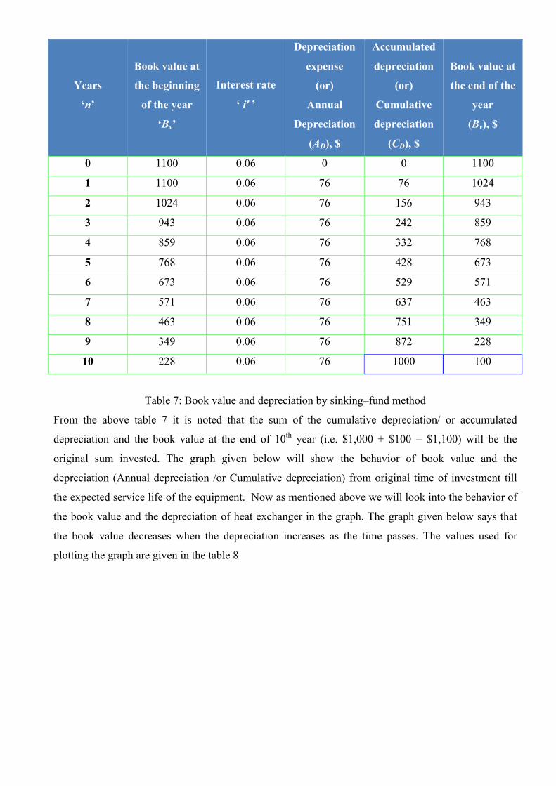
From the above table 7 it is noted that the sum of the cumulative depreciation/ or accumulated
depreciation and the book value at the end of 10th year (i.e. $1,000 + $100 = $1,100) will be the
original sum invested. The graph given below will show the behavior of book value and the
depreciation (Annual depreciation /or Cumulative depreciation) from original time of investment till
the expected service life of the equipment. Now as mentioned above we will look into the behavior of
the book value and the depreciation of heat exchanger in the graph. The graph given below says that
the book value decreases when the depreciation increases as the time passes. The values used for
plotting the graph are given in the table 8
Years
‘n’
Book value at
the end of the
year
(Bv), $
Accumulated
depreciation
(or)
Cumulative
depreciation
(CD), $
0 1100 0
1 1024 76
2 943 156
3 859 242
4 768 332
5 673 428
6 571 529
7 463 637
8 349 751
9 228 872
10 100 1000
Table 8. Book value and Depreciation by Sinking-fund method
0
200
400
600
800
1000
1200
0
200
400
600
800
1000
1200
0 1 2 3 4 5 6 7 8 9 10
Dep
reci
atio
n, $
Book Value, $
Years, n
Depreciation by sinking-‐fund method
Book Value Depreciation
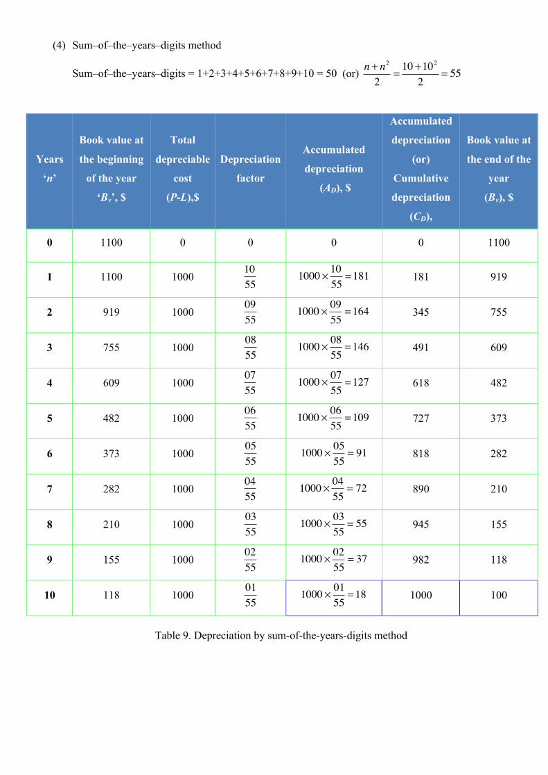
(4) Sum–of–the–years–digits method
Sum–of–the–years–digits = 1+2+3+4+5+6+7+8+9+10 = 50 (or) n + n2
2= 10 +10
2
2= 55
Years
‘n’
Book value at
the beginning
of the year
‘Bv’, $
Total
depreciable
cost
(P-L),$
Depreciation
factor
Accumulated
depreciation
(AD), $
Accumulated
depreciation
(or)
Cumulative
depreciation
(CD),
Book value at
the end of the
year
(Bv), $
0 1100 0 0 0 0 1100
1 1100 1000 1055
1000 ! 1055
=181 181 919
2 919 1000 0955
1000 ! 0955
=164 345 755
3 755 1000 0855
1000 ! 0855
=146 491 609
4 609 1000 0755
1000 ! 0755
=127 618 482
5 482 1000 0655
1000 ! 0655
=109 727 373
6 373 1000 0555
1000 ! 0555
= 91 818 282
7 282 1000 0455
1000 ! 0455
= 72 890 210
8 210 1000 0355
1000 ! 0355
= 55 945 155
9 155 1000 0255
1000 ! 0255
= 37 982 118
10 118 1000 0155
1000 ! 0155
=18 1000 100
Table 9. Depreciation by sum-of-the-years-digits method
Years
‘n’
Book value at
the end of the year
(Bv), $
Accumulated
depreciation
(or)
Cumulative
depreciation
(CD),
0 1100 0
1 919 181
2 755 345
3 609 491
4 482 618
5 373 727
6 282 818
7 210 890
8 155 945
9 118 982
10 100 1000
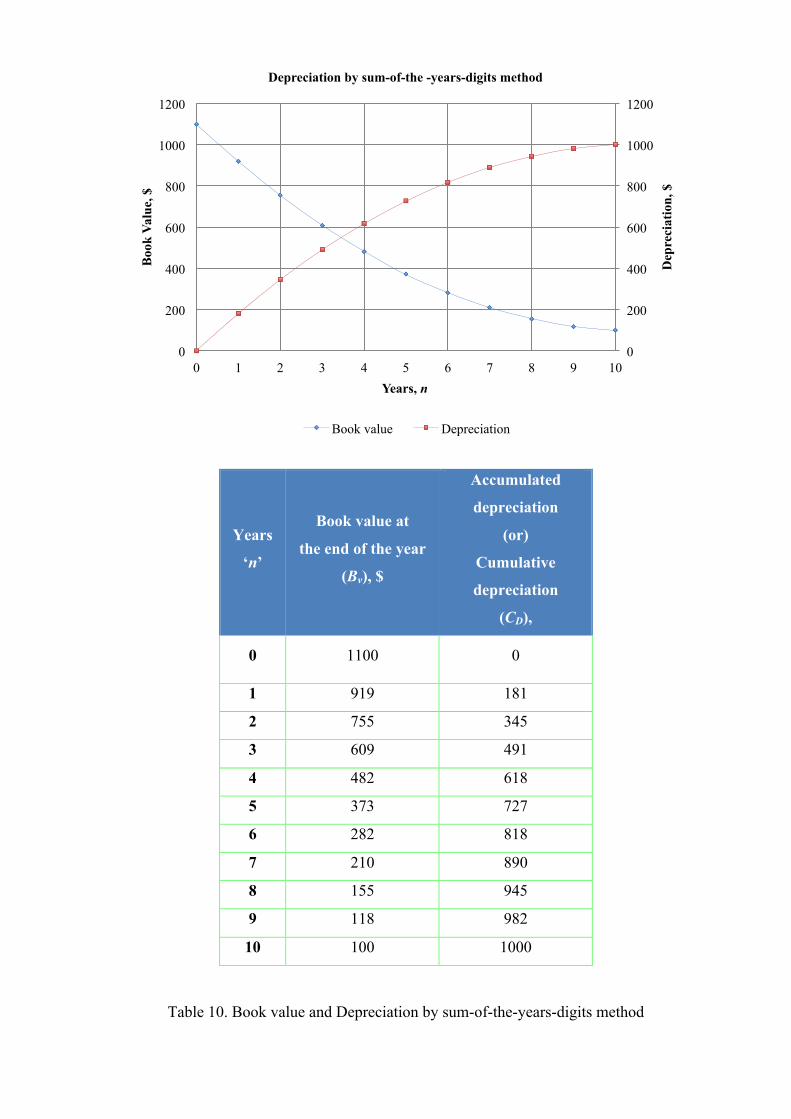
Table 10. Book value and Depreciation by sum-of-the-years-digits method
0
200
400
600
800
1000
1200
0
200
400
600
800
1000
1200
0 1 2 3 4 5 6 7 8 9 10
Dep
reci
atio
n, $
Boo
k Va
lue,
$
Years, n
Depreciation by sum-of-the -years-digits method
Book value Depreciation
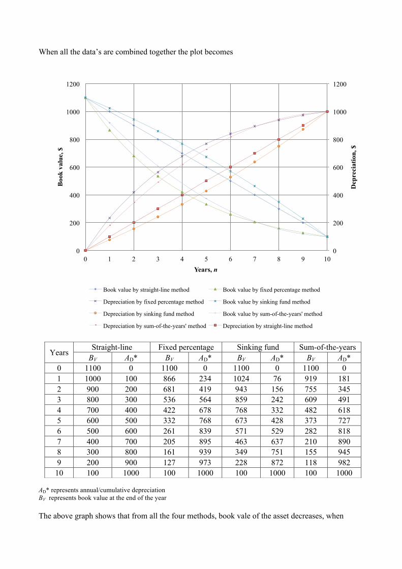
When all the data’s are combined together the plot becomes
AD* represents annual/cumulative depreciation BV represents book value at the end of the year The above graph shows that from all the four methods, book vale of the asset decreases, when
0
200
400
600
800
1000
1200
0
200
400
600
800
1000
1200
0 1 2 3 4 5 6 7 8 9 10
Dep
reci
atio
n, $
Boo
k va
lue,
$
Years, n
Book value by straight-line method Book value by fixed percentage method
Depreciation by fixed percentage method Book value by sinking fund method
Depreciation by sinking fund method Book value by sum-of-the-years' method
Depreciation by sum-of-the-years' method Depreciation by straight-line method
Years Straight-line Fixed percentage Sinking fund Sum-of-the-years
BV AD* BV AD* BV AD* BV AD* 0 1100 0 1100 0 1100 0 1100 0 1 1000 100 866 234 1024 76 919 181 2 900 200 681 419 943 156 755 345 3 800 300 536 564 859 242 609 491 4 700 400 422 678 768 332 482 618 5 600 500 332 768 673 428 373 727 6 500 600 261 839 571 529 282 818 7 400 700 205 895 463 637 210 890 8 300 800 161 939 349 751 155 945 9 200 900 127 973 228 872 118 982 10 100 1000 100 1000 100 1000 100 1000
depreciation of the asset increases. Similarly, the sum of annual/cumulative depreciation and book
value at the end of the year in all the four methods will be the original investment of the asset
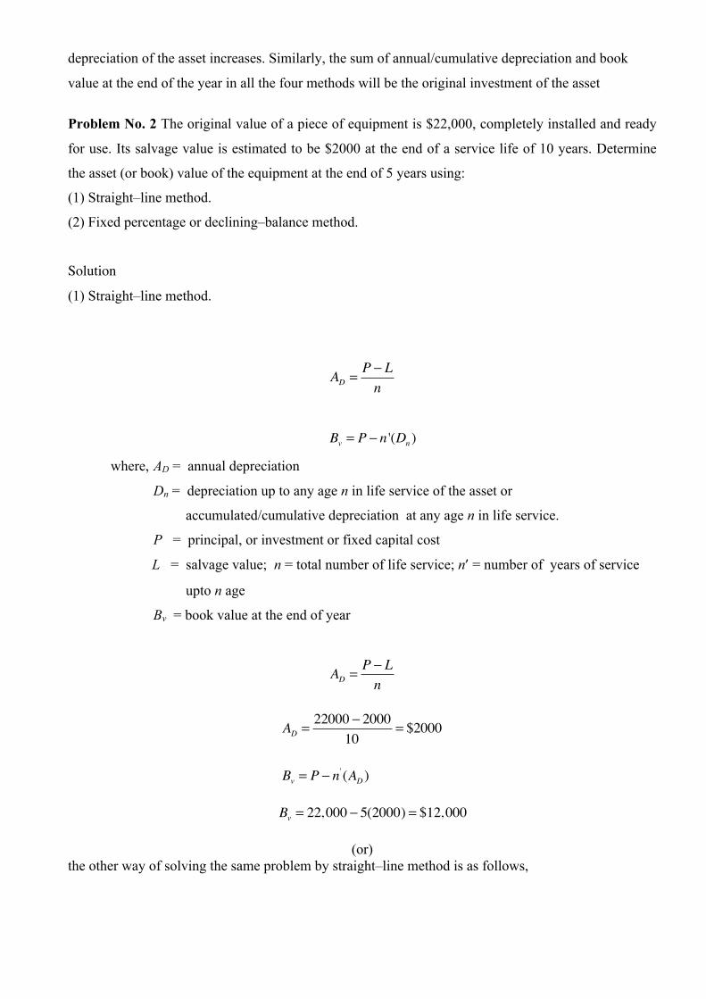
Problem No. 2 The original value of a piece of equipment is $22,000, completely installed and ready
for use. Its salvage value is estimated to be $2000 at the end of a service life of 10 years. Determine
the asset (or book) value of the equipment at the end of 5 years using:
(1) Straight–line method.
(2) Fixed percentage or declining–balance method.
Solution
(1) Straight–line method.
where, AD = annual depreciation
Dn = depreciation up to any age n in life service of the asset or
accumulated/cumulative depreciation at any age n in life service.
P = principal, or investment or fixed capital cost
L = salvage value; n = total number of life service; n’ = number of years of service
upto n age
Bv = book value at the end of year
AD = 22000 ! 200010
= $2000
Bv = P ! n ' (AD ) Bv = 22,000 ! 5(2000) = $12,000
(or) the other way of solving the same problem by straight–line method is as follows,
AD = P ! Ln
Bv = P ! n '(Dn )
AD = P ! Ln
where, AD = annual depreciation
Dn = depreciation up to any age n in life service of the asset or
accumulated/cumulative depreciation at any age n in life service.
P = principal, or investment or fixed capital cost
L = salvage value; n = total number of life service; n’ = number of years of service
upto n age
Bv = book value at the end of year
D1 =1(22, 000 ! 2000)
10= $2000
D2 =2(22, 000 ! 2000)
10= $4,000
D3 =3(22, 000 ! 2000)
10= $6,000
D4 =4(22, 000 ! 2000)
10= $8,000
D5 =5(22, 000 ! 2000)
10= $10,000
B1 = 22,000 !1(2000) = $20,000B2 = 22,000 ! 2(2000) = $18,000B3 = 22,000 ! 3(2000) = $16,000B4 = 22,000 ! 4(2000) = $14,000B5 = 22,000 ! 5(2000) = $12,000
B1 = 22,000 !1(2000) = $20,000B2 = 22,000 ! 2(2000) = $18,000B3 = 22,000 ! 3(2000) = $16,000B4 = 22,000 ! 4(2000) = $14,000B5 = 22,000 ! 5(2000) = $12,000
(2) Fixed percentage or declining–balance method.
Dn =n '(P ! L)
n
Bv = P ! n '(Dn )
Dn =n '(P ! L)
n
Bv = P ! n '(Dn )
f =1! LP
n
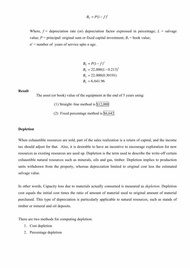
BV = P(1! f )n'
Where, f = depreciation rate (or) depreciation factor expressed in percentage; L = salvage
value; P = principal/ original sum or fixed capital investment; Bv = book value;
n’ = number of years of service upto n age.
BV = P(1! f )n
'
BV = 22,000(1! 0.213)5
BV = 22,000(0.30191)BV = 6,641.96
Result The asset (or book) value of the equipment at the end of 5 years using: (1) Straight–line method is $12,000
(2) Fixed percentage method is $6,642
Depletion
When exhaustible resources are sold, part of the sales realization is a return of capital, and the income
tax should adjust for that. Also, it is desirable to have an incentive to encourage exploration for new
resources as existing resources are used up. Depletion is the term used to describe the write-off certain
exhaustible natural resources such as minerals, oils and gas, timber. Depletion implies to production
units withdrawn from the property, whereas depreciation limited to original cost less the estimated
salvage value.
In other words, Capacity loss due to materials actually consumed is measured as depletion. Depletion
cost equals the initial cost times the ratio of amount of material used to original amount of material
purchased. This type of depreciation is particularly applicable to natural resources, such as stands of
timber or mineral and oil deposits.
There are two methods for computing depletion:
1. Cost depletion
2. Percentage depletion
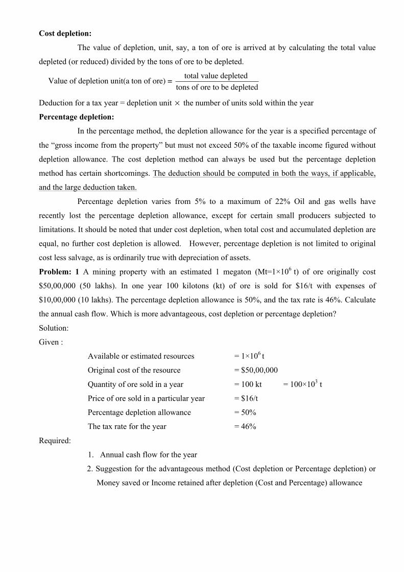
Cost depletion:
The value of depletion, unit, say, a ton of ore is arrived at by calculating the total value
depleted (or reduced) divided by the tons of ore to be depleted.
Value of depletion unit(a ton of ore) = total value depleted tons of ore to be depleted
Deduction for a tax year = depletion unit ! the number of units sold within the year
Percentage depletion:
In the percentage method, the depletion allowance for the year is a specified percentage of
the “gross income from the property” but must not exceed 50% of the taxable income figured without
depletion allowance. The cost depletion method can always be used but the percentage depletion
method has certain shortcomings. The deduction should be computed in both the ways, if applicable,
and the large deduction taken.
Percentage depletion varies from 5% to a maximum of 22% Oil and gas wells have
recently lost the percentage depletion allowance, except for certain small producers subjected to
limitations. It should be noted that under cost depletion, when total cost and accumulated depletion are
equal, no further cost depletion is allowed. However, percentage depletion is not limited to original
cost less salvage, as is ordinarily true with depreciation of assets.
Problem: 1 A mining property with an estimated 1 megaton (Mt=1×10⁶ t) of ore originally cost
$50,00,000 (50 lakhs). In one year 100 kilotons (kt) of ore is sold for $16/t with expenses of
$10,00,000 (10 lakhs). The percentage depletion allowance is 50%, and the tax rate is 46%. Calculate
the annual cash flow. Which is more advantageous, cost depletion or percentage depletion?
Solution:
Given :
Available or estimated resources = 1×10⁶ t
Original cost of the resource = $50,00,000
Quantity of ore sold in a year = 100 kt = 100×103 t
Price of ore sold in a particular year = $16/t
Percentage depletion allowance = 50%
The tax rate for the year = 46%
Required:
1. Annual cash flow for the year
2. Suggestion for the advantageous method (Cost depletion or Percentage depletion) or
Money saved or Income retained after depletion (Cost and Percentage) allowance
Calculation:
Cost depletion = Value of depletion unit(a ton of ore) = total value depleted tons of ore to be depleted
= 50, 00, 000
10, 00, 000= $5t
Price of ore sold in a year = $16 t
1 ton = $16
100 !103 ton = 100 !103t ! $161t
= 100 !103 !16 = $16,00,000
Gross income on the saleof 100 kt of ore
"#$= $16, 00, 000
Particulars Cost depletion Percentage depletion
1. Gross income $16,00,000.00 $16,00,000.00
2. Expenses for the year,
excluding depletion
$10,00,000.00 $10,00,000.00
3. Gross income after expenses,
taxable income [1 – 2]
$6,00,000.00 $6,00,000.00
4. (a) Cost of depletion at $5/t
for 100 kt i.e 1t = $5 for
100 kt it is = $5,00,000.00
$5,00,000.00 NA*
4. (b) Percentage depletion, at 50%
i.e. 50% of [3]
NA* $3,00,000.00
5. Actual income after the above
deductions [cost and
percentage depletion] or
actual taxable income
[3 – 4a]
$1,00,000.00 $3,00,000.00
[3 – 4b]
6. Tax at 46% on actual income $46,000.00 $1,38,000.00
7. Net cash flow or Available cash
after all tax deduction [3 – 6]
$5,54,000.00 $4,62,000.00
*NA – Not Applicable
Therefore, the cost depletion is advantageous that the percentage depletion.
since the larger deduction is usually taken into account as mentioned above.
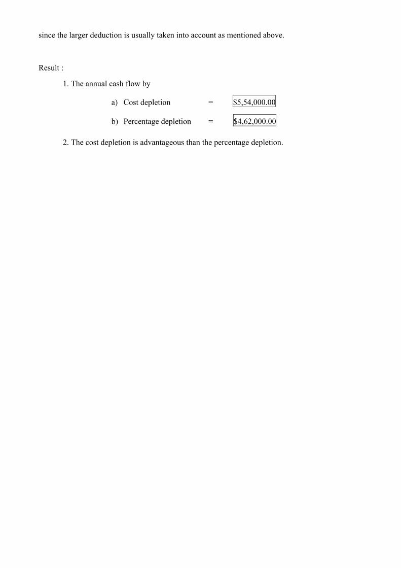
Result :
1. The annual cash flow by
a) Cost depletion = $5,54,000.00
b) Percentage depletion = $4,62,000.00
2. The cost depletion is advantageous than the percentage depletion.