american economic association - depfe unam · 2016-08-08 · nelson: the low-level equilibrium trap...

American Economic Association

A Theory of the Low-Level Equilibrium Trap in Underdeveloped EconomiesAuthor(s): Richard R. NelsonSource: The American Economic Review, Vol. 46, No. 5 (Dec., 1956), pp. 894-908Published by: American Economic AssociationStable URL: http://www.jstor.org/stable/1811910Accessed: 02/08/2010 15:17

Your use of the JSTOR archive indicates your acceptance of JSTOR's Terms and Conditions of Use, available athttp://www.jstor.org/page/info/about/policies/terms.jsp. JSTOR's Terms and Conditions of Use provides, in part, that unlessyou have obtained prior permission, you may not download an entire issue of a journal or multiple copies of articles, and youmay use content in the JSTOR archive only for your personal, non-commercial use.

Please contact the publisher regarding any further use of this work. Publisher contact information may be obtained athttp://www.jstor.org/action/showPublisher?publisherCode=aea.

Each copy of any part of a JSTOR transmission must contain the same copyright notice that appears on the screen or printedpage of such transmission.

JSTOR is a not-for-profit service that helps scholars, researchers, and students discover, use, and build upon a wide range ofcontent in a trusted digital archive. We use information technology and tools to increase productivity and facilitate new formsof scholarship. For more information about JSTOR, please contact [email protected].

American Economic Association is collaborating with JSTOR to digitize, preserve and extend access to TheAmerican Economic Review.

http://www.jstor.org

http://www.jstor.org/stable/1811910?origin=JSTOR-pdf

http://www.jstor.org/page/info/about/policies/terms.jsp

http://www.jstor.org/action/showPublisher?publisherCode=aea

A THEORY OF THE LOW-LEVEL EQUILIBRIUM TRAP IN UNDERDEVELOPED ECONOMIES

By RICHARD R. NELSON*

The malady of many underdeveloped economies can be diagnosed as a stable equilibrium level of per capita income at or close to subsistence requirements. Only a small percentage, if any, of the economy's income is directed toward net investment. If the capital stock is accumulating, population is rising at a rate equally fast; thus the amount of capital equipment per worker is not increasing. If economic growth is defined as rising per capita income, these economies are not growing. They_are caught in a low-level equilibrium trap. The purpose of this paper is to present a t',heteoryy of the nature'of the low- level equilibrium trap. The model is offered as a framework within which to analyze the problem7 of stagnant economies rather than as a model the parameters of whicY are to be statistically estimated. It is far too blunt an instrument for statistically refined methods of testing.'

Although the concept of low-level stagnation is scarcely new and different it is hoped that this paper does more than express the common knowledge of economists in a complicated manner. To the extent that the assumptions are realistic, the model provides a tool for analysis of the effects of various policies; and certain pitfalls that are not intui- tively obvious are brought to light. The model shows that, even if production techniques are not improved and even -'in the absence of a ~rash 7neiYstmentjir6gram, the trip may stl e'b escaped if'the socio- PO11t1Cdal environment iS favorable.

I. Assumptions and Definitions Three equations comprise the model: (1)Ar& equation explaining

changes in income, (2) au,equation explaining the quantity of net capital formation, and (3) an equation explaining population growth. The

* This paper is a summary of the theoretical sections of a thesis submitted in candidacy for a Ph.D. in economics at Yale University, 1956. The work was written under the direc- tion of Professors Henry Bruton, William Fellner and James Tobin. The author is assistant professor of economics at Oberlin College.

'While this paper was being written Harvey Leibenstein's book, "A Theory of Economic Demographic Development," was published. His model and the present one are similar in many respects.

NELSON: THE LOW-LEVEL EQUILIBRIUM TRAP 895

equations imply assumptions about technology and about human be- havior.

A. Changes in Income Income is the net gregate supply of want-satisfying goods dist

uted in a period of time and is a scalar quan0iy,iy measured in deflated monney. units. Given the social-political environment and eisting technology, income is assumed to be a linear homogeneous function of two variables, capital and labor. If both capital and labor are increased n-fold, and 1i there is no change in techniques, income produced increases n-fold.

1) Y = Af(K, P); nY = Af(nK, uP)

(Y = income, K = capital stock, P population, A an index of productivity, a constant if technology is constant.) Inputs of factors not explicitly included in equation (1) are assumed proportional to the input of either capital or population and therefore may be omitted from the function.

Capital,like income, is a scalar quantity valued in deflated money units. Population is a number. In the specific production function used in the appendix (Y AKaPia) popula :on is multiplied by capital and so the equation is dimensionally consistent.

The Population Input. The labor input is assumed to be a constant percentage of the population, given the social-political environment. The omission of the constant multiplier in equation (1) does not affect the analysis, and permits simpler notation.

The Capital Input. Capital consists of produced goods and arable land used in the production process. Land and produced capital are perfectly substitutable in the production of aggregate income. In other words, n money units of land, and n money units of produced capital can produce either the same product, or different products valued equally.

The Social and Technological Environment. The assumption of linear homogeneity is reasonable only if the social structure and the technology used are constant. Cultural inertia is conducive to economic inertia. But the reverse is also true. XVhere economies are stagnant, where capital is not accumulating, cultural rigidity is encouraged by a rigid economic circular flow.

Improved use of existing resources, either by fuller utilization of available inputs or by use of better alternative techniques, enables greater income from given inputs. Economies caught in the low-level equilibrium trap are often marked by considerable slack; that is, existing inputs are not producing the maximum amount of output that man's

896 THE AMERICAN ECONOMIC REVIEW

knowledge will allow. If these economies are properly stimulated, income may be increased with no increase in factor supplies. Increase in the productivity of existing factor supplies may be defined as innova- t-1on and is represented in the model by an increase in A in equation (1).

B. Net Capital Formation Net capital formation is an increase in the quantity of the capital

input of the production function. In the model there are two sources of capital formation: capital may be created out of curent income at the alternative cost of consumption, and, if there is unused arable land, capital may be increased by bringing this land under cultivation. Land and savings are valued in deflated money units.

(2) dK = dK'+ dL

(K = capital, K' savings-created capital, L land under cultivation.)

Land. The rate at which additional deflated money units of land are brought under cultivation is positively related to the increase in population, negatively related to the proportion of total arable land already under cultivation.

/L* -L\ (3) dL = g(L* )dP

(L = land under cultivation, L* total arable land, P = population.) As land area under cultivation inceases, the difficulty of bringing into cultivation additional land units of equal productivity increases.

Reproducible Capital. Per capita savings are determined by per capita income, and all savings flow into investment. Keynesian un- empoym enttof lahor an-d-'capiitT-is" pIenHThoienh of a money-market economy of specialized producers. The theory is not appropiate to an economy based on self-sufficient units, with'money and thX market playing but a minor role. Foreign investment is autonomous. The per capita rate of investment from savings, then, is determined as follows:

dK' b(Y/P - X); Y/P> (Y/P)' (4a)__=.

P . -C ; Y/P (Y/P)'

or

dK' b-bX (P/Y); Y/P > (Y/P)'

Y -C(P/Y) ; Y/P <` (Y/P)'

(K' investment from savings, X the zero savings level of Y/P, (Y/P)' the level of per capita income below which the rate of net disinvestment is the maximum technically possible.)


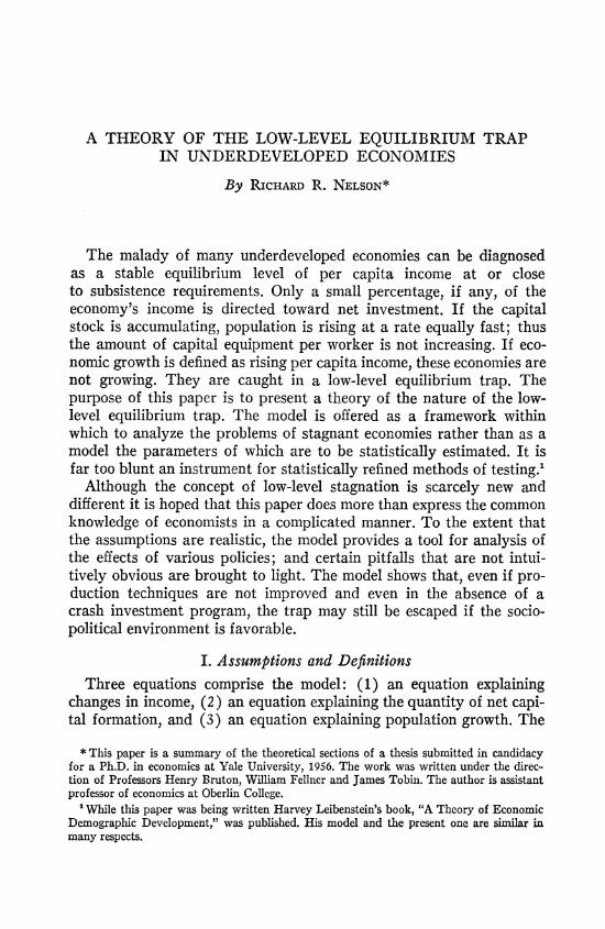
Until a certain level of per capita income is reached, all income will be spent on the necessities of life; hence the positive X-intercept (see Figure 1). Negative investment is limited by the rate of depreciation of the capital stock and the incentive to tear down existing equipment; hence the break in the function at (Y/P)'. One cannot eat torn-up railroad track no matter how hungry one may be. There is a maximum rate of capital depletion. (Soil depletion through failure to6-apply 'ferti- lizer is a principal source of capital depletion in poor agricultural economies.)

Changes in the distribution of income shift the dK'/P function to the right along the Y/P axis if the change is toward greater equality.

P'

0

FIGURE 1

The more unequal the income distribution, the lower the level of per capita income that is sufficient to support a given level of positive savingfGovternment apoicy may force capital formation from an economy with a per capita income so low that no investment would be forthcoming in the absence of 'government policy. Changes in government policy, distribution of income, and the social incentive system shift the dK'/P curve along the Y/P axis.

C. Population Growth Expressed as a formula, the rate of population growth is simply the

birth rate minus the death rate plus the rate of net immigration. For the purposes of the present model immigration is autonomous.

The neo-Malthusian assumptions about population growth are made. In areas with low per capita incomes short-run changes in the rate of population growth are caused by changes in the death rate, and changes in the death rate are caused by changes in the level of per capita income. Yet once per capita income reaches a level well above subsistence requirements, further increases in per capita income have a negligible


effect on the death rate. Since this is a short-run model, effects on the birth rate of a high, sustained per capita income are ignored. Hence:

dP p(Y/P-S); Y/P < (Y/P)"

P (dP/P)* ; Y/P ? (Y/P)"

(S subsistence level of per capita income, (dP/P) * -maximum rate of population growth, (YIP)" = level of per capita income above which increases in per capita income have negligible effect on the death rate.) The sharp break in the function is artificial but simplifies expo- sition (see Figure 2).

This function assumes a given income distributiony<given social structure, and givew- medical techniques. A shift in income distribution toward greater equality shifts the dP/P function to the left along the

p

0 (?)

FIGURE 2

YIP axis. The more unequal the income distribution, the smaller the population a given aggregate income can support.

The introduction of modern medical practices in certain areas since the second world war has enabled a sharp cut in the death rate; yet nutrition and housing standards have fallen sharply in some of these areas. If the death rate is viewed as a function of per capita income, then improved medical technique should be viewed as shifting the function to the left.

These assumptions are the basis of the trap model. Clearly, the model is designed to examine the short runj Any substantial sustained

per capitalncome certainly generates social change, and as the social-political structure changes the functions shift.

II. The Low-Level Equilibrium Trap The assumptions imply certain shapes of the dY/Y and dP/P curves

plotted against the Y/P axis. Given the state of technology, the quan-


tity_of unused land, and the social-political environment, dY/Y and dP/P are uniquely determined by the level of per capita income.

T1hmreaiWegro I of income, dY/Y, is explained by the equation:

dY 0Y dK aY dP y OKY Olp Y

(6) Y A Y dP P - -(dK'/Y + dL/PP/Y) + -

Since dK'/Y, dL/P and dP/P are determined by the level of per capita income through equations (3), (4) and (5), if WY/1K and 6Y/6P are determined by Y/P, then dY/Y is certainly determined by Y/P. If the production function is linear homogeneous, per capita income (Y/P) is uniquely determined by the capital-labor ratio (K/P), and the marginal productivities of capital and labor (WY/6K, 6Y/6P) are determined by the ratio of capital to labor (K/P). Thus, both the dY/Y and the dP/P curves are fixed over the Y/P axis.

If the level of per capita income that generates a zero rate of capital growth is also the suibsistence level of income (if S = X), then dY/Y and dP/P both equal zero at the subsistence level of per capita income (see Figure 3a). If the zero-investment level of per capita income exceeds the subsistence level of per capita income (if X exceeds S), then dY/Y is negative at S, and equals zero some point to the right of S and to the left of X (see Figure 3b). At this point the increase in income caused by a rising labor force is just offset by the decrease in income caused by a declining capital stock. If X is less than S, then the zero dY/Y level of per capita income is to the left of S and to the right of X.

To the right of its zero value the dY/Y curve rises with increasing per capita income as dP/P, the rate of population gr6wth, and dK'/Y, savings as a fraction of income, increase. As per capita income further increases, dP/P becomes a constant, and savings as a percentage of income approaches a constant; hence the dY/Y curve flattens out.

As per capita income rises still higher, the dY/Y curve may turn down. If the production function is linear homogeneous, the greater per capita income, Y/P, the smaller must be the output-capital ratio, Y/K, and since dK/Y approaches a constant, the proportional rate of growth of capital, dK/K- (Y/K) - (dK/Y), will tend to fall as per capita income increases. Since dP/P is a constant, dY/Y will tend to fall.2

If the rate of growth of income exceeds the rate of growth of popula- 2 dk/Y = dK'/Y + dL/P * P/Y. Since both dK'/Y and dL/P approach a constant as

YIP increases, if dL is large relative to dK', dK/Y may fall as YIP gets large.


tion (if the dY/Y curve lies above the dP/P curve at a given level of Y/P) then per capita income will increase from that level. Conversely, if the dP/P curve lies above the dY/Y curve at a given level of Y/P, then per capita income will fall from that level. Levels of per capita income at which dY/Y equals dP/P are equilibrium levels of per capita income. Population and income grow at an equal rate (positive, negative or zero) at that level of per capita income. However, an intersection of the dY/Y and dP/P curves will only be a stable equilibrium level of per capita income if the slope of the population growth curve exceeds the slope of the income growth curve at the intersection. If the dP/P curve lies above the dY/Y curve to the right of the intersection, below it to the left of the intersection (Y/P S and Y/P (Y/P)**

p

FIGuRE 3a

in Figure 3a), then if per capita income increases above the equilibrium level the increase in population will exceed that of income and per capita income will fall back toward the equilibrium. If per capita income falls below the equilibrium value, the rate of population growth will drop below the rate of income growth and per capita income will climb back toward the equilibrium. Conversely; if the slope of the dY/Y curve exceeds the slope of the dP/P curve at an equilibrium level of Y/P, the equilibrium is unstable (Y/P = (Y/P)* in Figure 3a), and deviations from that level will tend to grow. This is not economics but simple mathematics.

The low-level equilibrium trap is a phenomenon caused by the shape of the dY/Y and dP/P curves at their point of intersection at or in the neighborhood of S, the subsistence level of per capita income. This low-level equilibrium will henceforth be symbolized as (Y/P)t (where t means trap). Economies whose social, political and economic organ- ization generate a dP/P curve that exceeds in slope the dY/Y curve at (Y/P)t are caught in a low-level equilibrium trap-the equilibrum is stable. But there is no reason why the intersection (Y/P)t need be or remain a stable equilibrium. If the social, political and economic conditions generate a dY/Y curve of greater slope than the dP/P curve


at (Y/P) t, then there is no tendency for an economy to stagnate at the low-level equilibrium.

Translating from mathematics to economics, what conditions lead to a low-level equilibrium trap? If the production function is linear homogeneous, then output per capita can only be increased if the amount of capital per worker is increased. In other words, the dY/Y curve lies above the dP/P curve at a given level of per capita income if and only if the rate of capital increase exceeds the rate of population increase at that level of per capita income.

At an equilibrium level of per capita income both capital and population are constant, or are changing at an equal rate so that their ratio

d (dP/P) is constant. If the ratio d(dIP)at the equilibrium (Y/P) t is less than

d(dK/K) one, the equilibrium is unstable and there is no trap. If the ratio is greater than one, the economy is trapped at (Y/P)t. If S = X and dK/K = dP/P = 0 at (Y/P) t, then the ratio can be written:

K d'P K p (7)- _ __ _ _ _ _

P d2K P b -F g[(L* - L)/L*]p

where p, from equation (5), shows how responsive the rate of population growth is to changes in per capita income; b, from equation (4), is the marginal propensity to invest in per capita terms; (L*-L)/L*, from equation (3), is the percentage of total arable land that is still free and available for increased agricultural production, and g, from equation (3), is a measure of the propensity of new population to clear new arable land. The first fraction (K/P) summarizes the technological efficiency of the economy. The lower the ratio, the smaller the quantity of capital per laborer needed to support a given level of labor productivity. The second fraction:

p b + g[(L* - L)/L*]p

summarizes an economy's response to increases in per capita income from (Y/P)t. The lower the ratio, the greater the induced increase in capital relative to the induced increase in population. The greater the marginal propensity to invest, and the easier it is to bring new land into cultivation, the lower will be the ratio.

Thus, the social and technological conditions conducive to trapping an econo m y are: h.&i^gh cori5etIari n between& the- level of per capita income and the rate of population growth, (2) a low propensity to direct additional per capita income to increasing per capita investment, (3) scarcity of uncultivated arable land, and (4)inefficient production


methods. Opposite conditions are conducive to an unstable equilibrium at (Y/P)t. If the population maintains control over its rate of growth, if the propensity to invest is high and free land plentiful, and if production methods are efficient, then the economy will not be caught in the low-level equilibrium trap.

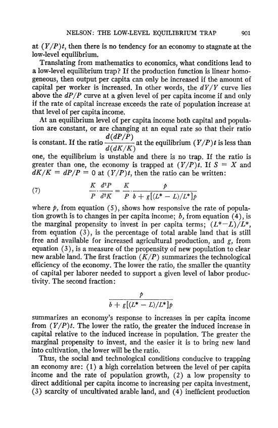
The Strength of the Trap. Assuming for the moment that the dY/Y and dP/P curves are-shap..ed' so as to trap the economy at (Y/P)t, the trap may be tight or loose. The strength of the trap is defined as the gap between (Y/P)t and (Y/P)*, the value of per capita income that must be achieved before the pull of the trap is escaped (Figure 3a). The relative values of S, the subsistence level of income, and X, the zero investment level of income, are important factors in determining the strength of the trap. If S is less than X, then the dP/P curve cuts

S (XP) L ( tyl~~~

FIGURE 3b

the Y/P axis to the left of the point where the dY/Y curve cuts the axis. In this case the gap between (Y/P)t and (Y/P)* is, of course, increased (Figure 3b). If X moves to the left, S to the right as income inequality increases, then, ceteris paribus, the more unequal the distribution of income, the weaker the hold of the trap.3

Improvement in medical technique and knowledge reduces the level of per capita income that is consistent with a stable population, and, according to the model, would seem to make escape from the trap more difficult. However, this effect may well be compensated for by the increase in labor productivity (shifting and lifting the dY/Y function) that better health may permit. This example points out an important implicit assumption of the model (and of many models): that param- eter values are assumed independent of each other.

Ceteris paribus, the smaller the difference between the slopes of the dP/P and dY/Y functions at (Y/P)t, the weaker the hold of the trap.

'The model neglects the stimulus that a mass smarket and the type of social structure that comes with greater equality of income distribution might have upon the propensity to invest and innovate.


The factors that act to trap an economy determine, in their degree, the tightness of the trap and the difficulty of escape.

The model suggests the tentative hypothesis that until the technological advances of the eighteenth and nineteenth centuries, rapid con- tinuous growth, such as that of the United States, Western Europe and Japan, could never have taken place, and only economies with ample free land (or that were exploiting colonies or subject states) could for long support a level of per capita incomie greater than (Y/P)t. (This is not to say that a small privileged class could not live in wealth.) Only economies with free land faced a dY/Y curve of greater slope than the dP/P curve at (Y/P)t. The state of technological knowledge necessitated a far larger amount of capital per laborer to support a given level of labor productivity than is needed with modern knowl-

K d2P edge. The ratio - d2K was large because K/P at (Y/P)t was large.

L*-L If free land (a large L* ) permitted easy capital accumulation,

a level of per capita income in excess of subsistence needs could be supported by productive agriculture, but as population increased and

L*-L crowded the land, would decrease and the dY/Y function

would pivot clockwise about S and (Y/P)t would become a stable equilibrium (see Figure 4). Once the land became crowded all econo-

FIGURE 4

mies were trapped. It has only been since the industrial revolution that man's knowledge has permitted densely populated economies to remain prosperous.

_The Escape from the Trap. The low-level equilibrium may be es- capedcln several ciTehrent ways. istorically, escape has been achieved through the simultaneous use of several means.


Changing social structure (a greater emphasis upon thrift and en- trep-rener-shp, greater incentives to produce in quantity, increased incentive to limit family size), increased percentage of the population in the labor force, changing distribution of income enabling accumulation of wealth by investors, a government investment program, all act to shift and pivot the income growth and population growth functions and thereby weaken the strength of the trap; perhaps eliminate the trap by pivoting the dY/Y curve to a greater slope than the dP/P curve at (Y/P)t. If this model summarizes the maladies of stagnant economies, then it is clear that policies directed toward eliminating social inertia may play an important role in loosening the trap.

Social and political change has usually been accompanied by appli- cation of improved production techniaues. The raising of the marginal productivity of capital and labor pivots the dY/Y function counter- clockwise. If the improvement in techniques is applied to all production, as well as to new production, then the taking up of slack lifts the dY/Y function over its entire range and enables an income increase that is achieved without increasing factor supplies. If the production function is written Y = Af(K, P), then dA/A, the proportional increase in productivity of existing factors of production, may be called the rate of innovation. The taking up of slack through innovation may provide the boost necessary to lift an economy out of the low-level equilibrium trap.

Increases in income and capital achieved through-funds obtained from_ abroad, an decreases in population through emigration can help to free an economy from the low-level equilibrium trap. However, small injections of funds may have no permanent effect unless accompanied by changing social-economic parameters, for unless the injection is sufficient to make dY/Y exceed dP/P the income increase will tend to be swamped by population increase. Of course, foreign assistance, to- gether with internal change, can play an important role in boosting an economy from the hold of the trap.

Growth after (Y/P)* is achieved. Once per capita income has increased beyond (Y/P) * growth will be self-generative, since (Y/P) * is an unstable equilibrium. Per capita income will either rise to a stable equilibrium value (Y/P)** if the dY/Y curve turns down to cut the dP/P curve from above; or, if the dY/Y curve stays above the dP/P curve (it need not turn down), per capita income will continuously increase. The gap between the dY/Y and dP/P curves determines the rate of growth of per capita income.

Thus, growth can be rapid and explosive if the dY/Y curve stays above the dP/P curve, or growth may be of the slow, shifting-equilibrium type. Through time, technological innovation may shift the


dY/Y function, and a decline in the birth rate may drop the dP/P function, thus shifting (Y/P)** to the right and accelerating growth. However, the model can only be, at best, suggestive of the determinants of the rate of growth of economies with a high per capita income.4

The Efect of Differential Rates of Response. The model is based on the assumption of a rapid response of population and net capital form- ationr to changes in the level of per capita income. Differential rates of response can affect the nature of the low-level equilibrium trap. If, after an increa-se-wper- cap-ta income, savings out of increased incomes are quickly directed toward capital creation which quickly starts new production, while population growth occurs only after a substantial time- lag, then the trap model is meaningless as a description of the world, and the model clearly does not explain stagnation. However, if the dP/P response occurs at the same speed, or with greater speed than the dY/Y response, then the different rates of response do not weaken the trap. The response of the death rate to increases in per capita income is probably rapid in areas where the level of per capita income is very low, and where death rates are high because of the low per capita income. On the other hand, income not consumed becomes productive only with a time-lag. Investment projects must be completed before income is created out of past increases in income. Differential rates of response are probably not of the sort that eliminate the low- level equilibrium trap.

'The assumptions of the model become increasingly unrealistic as per capita income increases above the subsistence level. The population growth function and the investment function clearly do not summarize the principal determinants of population growth and growth of capital stock in economies with a high per capita income. We then move into the Keynesian world, and Say's law is a poor tool. The assumption of a constant birth rate and a death rate responsive to small changes in per capita income likewise is inapplic- able in economies outside the trap range. Further, economies with a high level of per capita income are socially and technologically dynamic. Where population is growing and capital stock increasing, the social interrelationships and power equilibria are constantly changing. Economic change and cultural inertia are incompatible. If there is frequent social and technological change, the functions of the model are constantly shifting and the model becomes useless for analytic purposes. The assumption of a stable social-political system is also inappropriate to an economy with a per capita income below the subsistence level. Social and political upheaval has always been a concomitant of starvation. Hence, the mathematical curves of the model only have economic relevance in the neighborhood of the subsistence level of per capita income.

APPENDIX

The basic equations of the model are:

(1) Y = Af(K, P), nY = Af(nK, nP)

(Y = income, K = capital stock, P = population, A = index of productivity)


(2) dK = dL + dK'

L = land under cultivation, K' = capital from savings)

(3a) dK'/P = b(Y/P - X); Y/P > (Y/P)'

-c Y/P (Y/P)'

(X = zero savings level of per capita income)

(3b) dK'/Y = b - bX(P/Y); Y/P > (Y/P)'

- C(P/Y); Y/P < (Y/P)'

(4) dL = g[(L* - L)/L*]dP

(L* = total amount of arable land)

dP/P = p(Y/P - S); Y/P < (Y/P)"

(dP/P)* Y/P > (y/p)tf

(S = subsistence level of per capita income)

Differentiating (1) and using (2):

(6a) dY/Y = fk(dK'/Y + dL/Y) + fp(dP/Y) + dA/A

(6b) dY/Y = fk(dK'/Y + dL/P*P/Y) + fp(dP/P + P/Y) + dAIA

In order to give the model a firm shape that can be drawn, the Cobb- Douglas production function is used. However the essential argument holds for any linear homogeneous function.

(7) Y = AKapl-a

(8) dY/Y = dA/A + aA(K/P) a-1. (dK'/Y + dL/Y) + (1 - a)A(K/P)a dP/Y [from (7) and (6a)]

The following equations are useful for putting (8) in a more convenient form:

(9) YIP = A (K/P)a

(10) K/P = A-l1a(Y/p)l/a

(11) Y/K = A(K/P)a-1 = AlIa(y/p)(a-l),Ia

(8) may be rewritten:

(12) dY/Y = dAIA + aAlla(Y/p)(a-1)la(dK'/Y + dL/P P/Y)

+ (1 - a)dP/P; [from (10)] or as:

(13) dYlY = dA/A + adK/K + (1 - a)dP/P.

dY/Y = dA/A + [aAl1a(Y/P)(a-1)Ia][b -bX(P/Y)

+ (P/Y) g((L* - L)/L*)p(Y/P -S) ]


(14a) + (1 - a)p(Y/P -S); [from (10), (3b), (4) and (5)]

[(Y/P)' < Y/P < (YIP)"]

I assume that both S and X fall within this range of Y/P.

dY/Y = dA/A + aA la(Y/p)-11a [C+ g((L* -L)/L*) p(Y/P-s)]

(14b) +(1-a)p(Y/P-S);

[Y/P < (Y/P)']

dY/Y= dA/A+aA l/a(y/p)-(a-l)/a [b- bX(P/Y)]

(14c) + aA l/a(Y/p)-l1ag((L* - L)/L*) (dP/P)*+ (1-a) (dP/P)*;

[Y/P->-(Y/P)"]

From equation (14), dY/Y can be drawn over the Y/P axis. If L=L* and aA/A=0, then within the range (Y/P)'< Y/P<(Y/P)", dY/Y plotted against Y/P is negative at the lower bound, positive at the upper bound, and is a monotonically increasing function in between. The latter point is shown by differentiating (14a) with respect to Y/P and setting this equation equal to zero.

O9(dY/Y)/O (Y/P) = (a - 1)bA 1/a(Y/P)-l/a

(15a) + bXAlIa(Y/P)-lIa(P/Y) + (1 - a)p;

(dA/A = 0, L = L*) F-1 /a

bAl/a1 P

(15b) O(dY/Y)/O(Y/P) = 0 - YIP - [X/(i - a) ] y

\/a bA lIa() - p

The Y/P solution to 15b exceeds X/(1-a) and (Y/P)" exceeds X and so the dY/Y curve continuously increases in the range (Y/P)' < YIP <(Y/P)". In the range YIP> (Y/P)", Y/P reaches a maximum at YIP =X/(1-a), and approaches (1-a)(dP/P)* as YIP approaches infinity (from equation 14c).

The dY/Y cur-ve and the dP/P curve are shown plotted against the Y/P axis in Figure 3.

(16) d(Y/P) = dY/Y - dP/P

Thus when the dY/Y curve lies above the dP/P curve, YIP will rise, and conversely. Stability of an equilibrium value of Y/P (where dY/Y = dP/P) depends on the slopes of the curves at the intersection. If the slope of the dP/P curve exceeds the slope of the dY/Y curve the equilibrium is stable, otherwise unstable.

For any linear homogeneous function [nY =f(nK, nP) J YIP=g(K/P),


g'>O. This is shown by setting n=1/P. Thus at an equilibrium level of Y/P, dP/P = dK/K and the condition for stability can be written:

(17a) P >1 or

2 Pd2p- dp2 > 1

do /d() P Kd2K - dK 2

If S = X [(dP/P) = (dK/K) = 0] at the equilibrium then the condition for stability can be written:

(17b) K/P*d2P/d2K> 1

If L-L* this condition can be written [from equations (3) and (5)]:

(17c) KK/P*p/b > 1

Lc)L #L

If L# L* then for stability [from equations (3), (4), and (5)]

(17d) K/P.- p- > 1 b + g((L* - L)/L*)p

The basic analysis thus far has not been dependent on the use of the Cobb- Douglas function. Any linear homogeneous function gives rise to a similarly shaped curve in the neighborhood of S, and the stability conditions are general. However not every linear homogeneous function gives rise to a dY/Y curve that always dips down below the dP/P curve as YIP becomes great. For example, the dY/Y curve derived from the linear homogeneous function:

(18) Y = rK + wP,

and equations (3a) and 6 is:

(19) dY/Y = r[b - bX(P/Y)] + w(P/Y)(dP/P)*

(Y/P > (Y/P)", L = L*)

This curve approaches rb as Y/P goes to infinity, and there is no reason why rb may not exceed (dP/P)*.

american economic association - depfe unam · 2016-08-08 · nelson: the low-level equilibrium trap...

Documents