AMBIGUITY FUNCTION ANALYSIS AND DIRECT-PATH SIGNAL FILTERING OF THE DIGITAL AUDIO

BROADCAST (DAB) WAVEFORM FOR PASSIVE COHERENT LOCATION (PCL)

THESIS

Abdulkadir Guner, First Lieutenant, TUAF

AFIT/GE/ENG/02M-09

APPROVED FOR PUBLIC RELEASE; DISTRIBUTION UNLIMITED

Report Documentation Page

Report Date 15 Mar 02

Report Type Final

Dates Covered (from... to) Jun 2001 - Mar 2002

Title and Subtitle Ambiguity Function Analysis and Direct-Path SignalFiltering of the Digital Audio Broadcast (DAB)Waveform for Passive Coherent Location (PCL)

Contract Number

Grant Number

Program Element Number

Author(s) 1st Lt Abdulkadir Guner, TUAF

Project Number

Task Number

Work Unit Number

Performing Organization Name(s) and Address(es) Air Force Institute of Technology Graduate Schoolof Engineering and Management (AFIT/EN) 2950 PStreet, Bldg 640 WPAFB OH 45433-7765

Performing Organization Report Number AFIT/GE/ENG/02M-09

Sponsoring/Monitoring Agency Name(s) and Address(es) NATO C3 Agency ATTN: Dr Paul Howland P. O.Box 174 De Haag- The Netherlands

Sponsor/Monitor’s Acronym(s)

Sponsor/Monitor’s Report Number(s)

Distribution/Availability Statement Approved for public release, distribution unlimited

Supplementary Notes

Abstract This research presents an ambiguity function analysis of the digital audio broadcast (DAB) waveform andone signal detection approach based on signal space projection techniques that effectively filters thedirect-path signal from the receiver target channel. Currently, most Passive Coherent Location (PCL)research efforts are focused and based on frequency modulated (FM) radio broadcasts and analogtelevision (TV) waveforms. One active area of PCL research includes the search for new waveforms ofopportunity that can be exploited for PCL applications. As considered for this research, one possiblewaveform of opportunity is the European digital radio standard DAB. For this research, the DABperformance is analyzed for application as a PCL waveform of opportunity. For this analysis, DABambiguity function calculations and ambiguity surface plots are created and evaluated. Signal detectioncapability, to include characterization of time-delay and Doppler-shift measurement accuracy andresolution, is investigated and determined to be quite acceptable for the DAB waveform

Subject Terms Passive Radar, Passive Coherent Location System (PCL), Passive Sensor Location System, Bistatic Radar,Multistatic Radar, Digital Audio Broadcast (DAB), Adaptive Signal Filtering, Coded OrthogonalFrequency Division Multiplex (COFDM).

Report Classification unclassified

Classification of this page unclassified

Classification of Abstract unclassified

Limitation of Abstract UU

Number of Pages 128

ii

The views expressed in this document are those of the author and do not reflect the official

policy or position of the Turkish Air Force, Turkish Government, United States Air Force,

Department of Defense, United States Government, the corresponding agencies of any other

government, NATO, or any other defense organization.

This document represents the results of research based on information obtained solely

from open sources. No agency, whether United States Government or otherwise, provided any

threat system parameters, or weapons systems performance data in support of the research

documented herein.

iii

AFIT/GE/ENG/02M-09

AMBIGUITY FUNCTION ANALYSIS AND DIRECT-PATH SIGNAL FILTERING OF THE DIGITAL AUDIO BROADCAST (DAB) WAVEFORM FOR PASSIVE COHERENT LOCATION

(PCL)

THESIS

Presented to the Faculty

Department of Electrical and Computer Engineering

Graduate School of Engineering and Management

Air Force Institute of Technology

Air University

Air Education and Training Command

In Partial Fulfillment of the Requirements for the

Degree of Master of Science in Electrical Engineering

Abdulkadir Guner, B.S.E.E

First Lieutenant, TUAF

March 2002

APPROVED FOR PUBLIC RELEASE; DISTRIBUTION UNLIMITED

AFrr/GE/ENG/O2M-O9

AMBIGUITY FUNCTION ANALYSIS AND DIRECT -PATH SIGNAL FILTERING OF THEDIGITAL AUDIO BROADCAST (DAB) WAVEFORM FOR PASSIVE COHERENT LOCATION

(PCL)

Abdulkadir Guner, B.S.E.EFirst Lieutenant, TUAF

Approved:

I- 6t-c. -ov-- <t) ~Date

L:~--l=~~2:::::Michael A. Temple, Ph.J)f

Committee Chairman

~~=2 ~VAndrew Terzuoli, Ph.D.Committee Member

10 /l.( ~ '\-c)c)"\

Date

L~ /1//4J,fj 1Date

IV

v

TABLE OF CONTENTS

CHAPTER 1 INTRODUCTION .................................................................................................... 6

1.1 Background ..................................................................................................................... 6

1.2 Different PCL systems .................................................................................................... 9

1.3 Research problem statement ......................................................................................... 11

1.4 Assumptions.................................................................................................................. 12

1.5 Scope ............................................................................................................................. 13

1.6 Materials and equipment ............................................................................................... 13

1.7 Thesis organization ....................................................................................................... 13

CHAPTER 2 BACKGROUND .................................................................................................... 15

2.1 Introduction ................................................................................................................... 15

2.2 Analog TV and FM radio broadcast waveforms........................................................... 15

2.3 PCL Systems ................................................................................................................. 17

2.3.1 Manatash Ridge Radar (MRR).................................................................................. 17

2.3.2 Lockheed Martin’s Silent Sentry® PCL System [3]................................................. 18

2.3.3 TV Based Bistatic Radar [7-8] .................................................................................. 19

2.3.4 Other PCL Concepts.................................................................................................. 20

2.4 Digital Audio Broadcast (DAB) waveform .................................................................. 22

2.4.1 The COFDM Modulation Technique [20] ................................................................. 22

2.4.2 The DAB standard...................................................................................................... 28

2.5 Summary ....................................................................................................................... 36

CHAPTER 3 METHODOLOGY.................................................................................................. 37

3.1 Introduction ................................................................................................................... 37

vi

3.2 Ambiguity Function Analysis [12]................................................................................ 37

3.3 Ambiguity function analysis of the DAB waveform .................................................... 47

3.4 Practical issues with DAB-PCL system........................................................................ 52

3.5 Implementation of direct-path filter .............................................................................. 57

3.6 Summary ....................................................................................................................... 61

CHAPTER 4 SIMULATION RESULTS AND ANALYSIS....................................................... 62

4.1 Introduction ................................................................................................................... 62

4.2 Ambiguity function analysis of the DAB waveform .................................................... 62

4.3 DAB waveform performance evaluation ...................................................................... 72

4.4 DAB detection surfaces................................................................................................. 78

4.5 Direct signal filtering .................................................................................................... 84

4.6 Simulations.................................................................................................................... 87

4.6.1 Ideal case: Perfect phase references .......................................................................... 88

4.6.2 Realistic conditions: Imperfect phase references ...................................................... 90

4.7 Performance evaluation of direct-path filter ................................................................. 95

4.8 Summary ....................................................................................................................... 97

CHAPTER 5 CONCLUSIONS AND RECOMMENDATIONS ................................................. 99

5.1 Summary ....................................................................................................................... 99

5.2 Conclusions ................................................................................................................. 100

5.3 Recommendations for Future Research ...................................................................... 102

APPENDIX A – Acronyms......................................................................................................... 104

APPENDIX B – Simulation Code .............................................................................................. 106

1

TABLE OF FIGURES

Figure 2.1 Orthogonal subcarriers in OFDM

Figure 2.2 Effect of multipath using no signal during the guard interval

Figure 2.3 OFDM Symbol with Cyclic Prefix Insertion

Figure 2.4 Phasor representation of demodulated subcarriers (I-III)

Figure 2.5 Phasor representation of demodulated subcarriers (I-III) amplitude comparison

Figure 2.6 Amplitude comparison of sum phasor to reference phasor

Figure 3.1 Normalized Ambiguity Surface Plot for Rectangular Sinusoidal Pulse Carrier Frequency

kHzfc 40= and pulse duration sec0025.0=pt

Figure 3.2 Normalized Ambiguity Surface Plot for Rectangular Sinusoidal Pulse Carrier Frequency

kHzfc 40= and pulse duration sec005.0=pt

Figure 3.3 Zero Time Delay Doppler Frequency Axis, Rectangular Sinusoidal Pulse

Carrier Frequency kHzfc 40= and pulse duration sec0025.0=pt

Figure 3.4 Zero Time Delay Doppler Frequency Axis, Rectangular Sinusoidal Carrier

Carrier Frequency kHzfc 40= and pulse duration sec005.0=pt

Figure 3.5 Block Diagram of Direct Path Filter signal processing

Figure 4.1 DAB Symbol Bandwidth

Figure 4.2 Method 1: Independent Subcarrier Doppler, Zero Doppler DAB Ambiguity Surface Cut (30

Subcarriers and 20 Symbol Coherent Integration Time)

Figure 4.3 Method 2: Dependent Subcarrier Doppler, Zero Doppler DAB Ambiguity Surface Cut (30

Subcarriers and 20 Symbol Coherent Integration Time)

Figure 4.4 Difference Plot of Zero Doppler Ambiguity Surfaces Generated Using Independent and

Dependent Subcarrier Induced Doppler

2

Figure 4.5 Method 1: Independent Subcarrier Doppler, Zero Time-Delay DAB Ambiguity Surface Cut

(30 Subcarriers and 20 Symbol Coherent Integration Time)

Figure 4.6 Method 2: Dependent Subcarrier Doppler, Zero Time-Delay DAB Ambiguity Surface Cut (30

Subcarriers and 20 Symbol Coherent Integration Time)

Figure 4.7 Difference Plot of Zero Time-Delay Ambiguity Surfaces Generated Using Independent and

Dependent Subcarrier Induced Doppler

Figure 4.8 Ambiguity Surface of the DAB Waveform (15 Subcarriers and 10 Symbol Coherent

Integration Time)

Figure 4.9 Zero Doppler Ambiguity Surface Cut of the DAB Waveform (15 Subcarriers and 10 Symbol

Coherent Integration Time)

Figure 4.10 Zero Time-Delay Ambiguity Surface Cut of the DAB Waveform (15 Subcarriers and 10

Symbol Coherent Integration Time)

Figure 4.11 Zero Doppler Ambiguity Surface Cut of the DAB Waveform (75 Subcarriers and 50 Symbol

Coherent Integration Time)

Figure 4.12 Zero Time-Delay Cut of DAB Waveform Ambiguity Surface

Figure 4.13 Target Channel Detection Surface – Target Present (30 Subcarriers and 20 Symbol Coherent

Integration Time)

Figure 4.14 Target Channel Detection Surface – Target Present (30 Subcarriers and 20 Symbol Coherent

Integration Time)

Figure 4.15 Representative DAB Detection Surface Plot

Figure 4.16 Frequency Domain Response of DAB Direct Signal and Doppler Shifted Target Return

Figure 4.17 Post-Filtered Detection Surface Showing Detectable Target Response Ideal Scenario - Perfect

Symbol Phase Reference

Figure 4.18 Post-Filtered Detection Surface Showing Detectable Target Response Ideal Scenario - Perfect

Symbol Phase Reference

3

Figure 4.19 Pre-Filtered Detection Surface Showing Undetectable Target Response Non-Ideal Scenario -

Imperfect Symbol Phase Reference

Figure 4.20 Pre-Filtered Detection Surface Showing Undetectable Target Response Non-Ideal Scenario -

Imperfect Symbol Phase Reference (side view)

Figure 4.21 Post-Filtered Detection Surface Showing Detectable Target Response Non-Ideal Scenario -

Imperfect Symbol Phase Reference

Figure 4.22 Post-Filtered Detection Surface Showing Detectable Target Response Non-Ideal Scenario -

Imperfect Symbol Phase Reference (side view)

Figure 4.23 Spectral Filter Responses for DAB Signal

4

AFIT/GE/ENG/02M-09

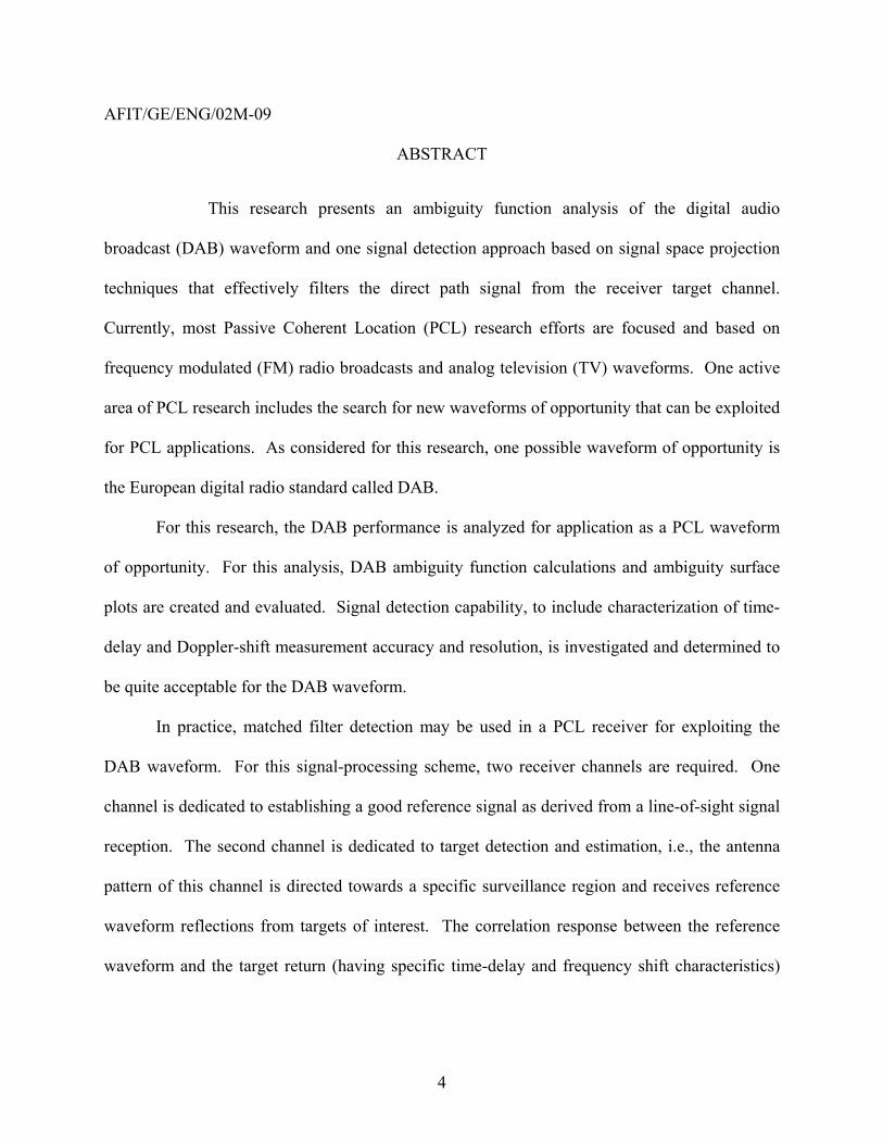
ABSTRACT

This research presents an ambiguity function analysis of the digital audio

broadcast (DAB) waveform and one signal detection approach based on signal space projection

techniques that effectively filters the direct path signal from the receiver target channel.

Currently, most Passive Coherent Location (PCL) research efforts are focused and based on

frequency modulated (FM) radio broadcasts and analog television (TV) waveforms. One active

area of PCL research includes the search for new waveforms of opportunity that can be exploited

for PCL applications. As considered for this research, one possible waveform of opportunity is

the European digital radio standard called DAB.

For this research, the DAB performance is analyzed for application as a PCL waveform

of opportunity. For this analysis, DAB ambiguity function calculations and ambiguity surface

plots are created and evaluated. Signal detection capability, to include characterization of time-

delay and Doppler-shift measurement accuracy and resolution, is investigated and determined to

be quite acceptable for the DAB waveform.

In practice, matched filter detection may be used in a PCL receiver for exploiting the

DAB waveform. For this signal-processing scheme, two receiver channels are required. One

channel is dedicated to establishing a good reference signal as derived from a line-of-sight signal

reception. The second channel is dedicated to target detection and estimation, i.e., the antenna

pattern of this channel is directed towards a specific surveillance region and receives reference

waveform reflections from targets of interest. The correlation response between the reference

waveform and the target return (having specific time-delay and frequency shift characteristics)

5

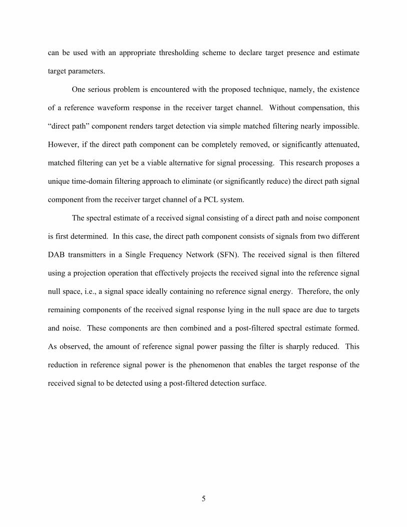
can be used with an appropriate thresholding scheme to declare target presence and estimate

target parameters.

One serious problem is encountered with the proposed technique, namely, the existence

of a reference waveform response in the receiver target channel. Without compensation, this

“direct path” component renders target detection via simple matched filtering nearly impossible.

However, if the direct path component can be completely removed, or significantly attenuated,

matched filtering can yet be a viable alternative for signal processing. This research proposes a

unique time-domain filtering approach to eliminate (or significantly reduce) the direct path signal

component from the receiver target channel of a PCL system.

The spectral estimate of a received signal consisting of a direct path and noise component

is first determined. In this case, the direct path component consists of signals from two different

DAB transmitters in a Single Frequency Network (SFN). The received signal is then filtered

using a projection operation that effectively projects the received signal into the reference signal

null space, i.e., a signal space ideally containing no reference signal energy. Therefore, the only

remaining components of the received signal response lying in the null space are due to targets

and noise. These components are then combined and a post-filtered spectral estimate formed.

As observed, the amount of reference signal power passing the filter is sharply reduced. This

reduction in reference signal power is the phenomenon that enables the target response of the

received signal to be detected using a post-filtered detection surface.

6

AMBIGUITY FUNCTION ANALYSIS AND DIRECT-PATH SIGNAL FILTERING OF THE DIGITAL AUDIO BROADCAST (DAB) WAVEFORM FOR PASSIVE COHERENT LOCATION

(PCL)

CHAPTER 1 INTRODUCTION

1.1 Background

In the radar world, the first task is to detect an object in a region of interest. In this

context the object to be detected is called a target. Following detection, we would like to

determine specific target parameters, such as position and velocity and if possible, we would like

to track the target and its related parameters. As a more challenging task, we would also like to

know what the target is, i.e., identify it as friend or foe.

Deployed radar systems employ many different techniques to achieve these goals. Many

send a signal specifically designed to enhance the signal processing tasks of detecting, tracking

and possibly identifying the target. The radar systems of concern for this work rely on target

radio frequency (RF) re-radiation, or scattering, characteristics to accomplish these tasks. For

passive coherent location (PCL), the original source of energy is derived from a waveform of

opportunity in the environment and the re-radiated energy from the target is processed.

Both active and passive target detection techniques have inherent problems associated

with them. Passive techniques, which rely on target RF emissions such as target radar or IFF

transmissions, can become ineffective in detecting targets which implement “emission control”

(EMCON) procedures. On the other hand, transmission of the special waveforms such as those

used in active radar systems, may be intercepted by the “Electronic Counter Measures” (ECM)

equipment aboard the platform. This means the target can detect the radar before the radar

detects the target.

7

Another problem with active radar systems is the need for allocated frequency spectrum

for transmission of the radar waveform. The frequency spectrum is already crowded with many

communication and broadcast applications. Radar waveform therefore, must be transmitted

within a limited frequency spectrum as dictated by other applications.

As a case in point, radars operating at “Very High Frequency” (VHF) are effective in

detecting hidden ground targets such as tanks in a forest. These radars also have a very high

range capability, which can be important for detecting ballistic targets. However, FM radios also

broadcast at VHF and can affect the performance of the radar significantly. In the end, the

benefits associated with VHF operation become questionable in a region filled with FM radio

transmissions [1].

In fact, the above described active and passive techniques are not the only available

detection methods. In 1978, IBM scientists came together in an attempt to enter the radar

market. As part of their effort, scientists looked for a means to enhance target detection and

tracking. There were several choices considered:

1. Monostatic active radar: In this technique, the radar transmits and receives a

waveform specialized to ease target detection and tracking processing. The transmitter

and receiver are collocated or are separated with a relatively small distance in comparison

to expected target distance. Practically speaking, these systems are vulnerable to “Anti

Radiation Missiles” (ARMs). Also, in the monostatic architecture, if the target platform

has an ECM system onboard, it is highly possible that the target platform can detect the

radar signal before the radar detects the target platform. In this case, the target platform

may avoid being detected.

8

2. Bistatic radar [2]: This technique requires one transmission from a distant

transmitter site. So, the transmitter and receiver are not collocated. In this case, the

transmitter is still vulnerable to ARM attack and the target platform with ECM capability

can still detect the presence of a radar and possibly avoid it.

3. Non-cooperative bistatic radar: This system uses transmissions from another radar

system, which may be either friendly or foe. In this case, the performance will be limited

since there is no control of the transmission. The advantage of this technique is that if the

original radar system is being jammed, this system will be minimally affected.

4. Electronic Support Measures (ESM): ESM are passive in nature and rely solely on

target platform transmissions for detection. It is relatively cheap to implement and

operates covertly since no transmissions are generated. However, ESM performance

diminishes when the target platform applies EMCON.

Last but not least, there are currently a significant number of RF transmissions present in

the environment designed for non-radar related purposes, e.g., TV and FM broadcasts or mobile

communication signals. Such signals may be exploited for detection, tracking and possible

identification of targets – this exploitation falls under the umbrella of PCL techniques. It was

this idea that was adopted by IBM radar researchers. This concept, called Passive Coherent

Location (PCL), is what lead to the development of the Silent Sentry® system by Lockheed

Martin and inspired the designs of many other systems around the world.

As indicated above, the PCL concept was introduced by researchers at IBM. There are

several PCL definitions available in the open literature. Lockheed Martin researchers define it as

a system, which uses everyday broadcast signals, such as those for television and radio, to

illuminate, detect and track targets [3]. Another PCL definition comes from NASA scientists

9

who work with Lockheed Martin colleagues in an effort to make tracking of launched space

vehicles cheaper. NASA defines a PCL system as one that capitalizes on the energy emitted by

commercial broadcast stations, such as radio or television networks. “Using a ground-based

system of antennas, receivers and signal processors, PCL tracks this energy as it is reflected off

an ascending launch vehicle, allowing its ascent trajectory to be plotted.”[4]. Another PCL

definition taken from the Journal of Electronic Defense, explains PCL as an electronic system

that tracks civilian radio and TV broadcast signals, detecting aircraft by analyzing the slight

disturbance in the commercial wavelengths caused by their flight [5].

1.2 Different PCL systems

The basic idea of PCL is clear; exploitation of existing RF emissions from broadcast or

communication signals in such a way to detect, track and also identify objects called targets.

Different approaches have been taken by researchers in determining which RF emissions should

be used in PCL applications. Most PCL literature is based on FM broadcasts and analog TV

signals [6-10]. The specific choice of a “waveform of opportunity” [11] greatly affects signal

processing of the system. For example, if one uses the audio or video carrier of an analog TV

signal [8], then a narrowband system is present and Doppler analysis can be performed along

with “Direction of Arrival” (DOA) measurements. Doppler and DOA measurements are used to

estimate the range, position and velocity of a target.

One can also estimate target parameters such as range, position and velocity through

“Time Difference Of Arrival” (TDOA) techniques. TDOA techniques are somewhat easier to

implement since matched filtering can be used to extract TDOA information from the received

signal. This may not be possible with an analog TV signal because of the waveform structure.

In an analog TV signal, there exists a synchronization frame. This short period synchronization

10

frame makes TDOA measurements ambiguous at approximately every 9.0 km [9]. There are

other available waveforms, such as an FM radio broadcast signal, which are viable for TDOA

processing. Here the bandwidth of the signal greatly affects measurement accuracy [12]. A

range resolution of 2.0 km has been achieved using FM broadcasts [9]. Silent Sentry® system,

the first off-the shelf commercially available PCL product in the world, uses FM broadcasts as

the waveform of opportunity [3].

Available waveforms of opportunity are not limited to only analog TV and FM

broadcasts. Many people have cell phones, which means a large number of mobile

communication signals are present in the environment. Other possibilities include digital TV or

digital radio broadcast. Many countries have decided to use digital broadcasts as future standard

for audio and video transmission. Although current usage is not very widespread, the audience of

digital broadcasts is steadily increasing and Europe is leading the world in this effort. For

example, the “Digital Audio Broadcast” (DAB) waveform, is a well-establish standard for digital

audio broadcasts and is starting to get popular. In Britain, 60% of the population has access to

DAB. In Germany, the rate is 30%, in France 25%, in Belgium 86%, in Sweden 85%, and in the

Netherlands 45%. In other countries such as Turkey, digital audio broadcast implementation is

in the planning phase [13].

Looking at the growing developments in the digital domain, especially in digital audio

broadcasting, one is lead to the possibility of using DAB waveform in PCL applications. An

encouraging fact is that the waveform standard, which can be found in open literature, is a

widely accepted standard in many countries. For Europe, the “European Telecommunications

Standards Institute” (ETSI) has issued a standard for digital audio broadcasting. The standards

11

are published in a document called ETS 300 401 [14]. The potential widespread use of DAB

makes it a waveform to be considered for possible PCL applications.

1.3 Research problem statement

The standard DAB signal with a bandwidth of approximately 1.5 MHz is viable for TDOA

calculations in a PCL application. In TDOA signal processing, matched filters can be used to

extract TDOA information from the received signal. Before building an actual system that

operates with DAB, it would be best to first test DAB waveform properties in a passive radar

scenario. One powerful analysis tool for characterizing the performance of any waveform in a

radar system with a matched filter receiver is the “Ambiguity function”. An “Ambiguity

Surface”, i.e., a two-dimensional plot of the ambiguity function, indicates what performance can

be expected from the waveform in question. As addressed under this research, waveform

performance characterization includes determining the achievable accuracy and resolution in

time-delay and Doppler shift measurements of the received waveform.

Making TDOA measurements with a PCL system requires a minimum of two receiver

channels. The “reference channel” is dedicated to receiving and generating a reference signal to

be used in matched filtering. The reference signal is the direct break-through of the broadcast

transmitter arriving at the receiver along a line-of-sight path. The second channel, the “target

channel” is dedicated to receiving returns of the transmitted waveform of opportunity that have

reflected from objects (targets) in the environment. Matched filtering in PCL applications

includes cross-correlating received signals in both channels.

One problem with this matched filtering process arises from the fact that the channels are

not perfectly isolated, i.e., one component in the reference channel is the target return.

Additionally there is a leakage from the reference signal component into the target channel. The

12

effect of the reference signal response in the target channel is more severe mainly because the

reference signal arrives at the receiver with much higher power than the target return. The

effects of this leakage have been addressed in literature [11]. The reference signal component in

the target channel causes false detection in the receiver, unless this component can be removed

or significantly reduced.

This research proposes a unique time-domain filter to remove or significantly reduce the

reference signal component in the target channel. The analytical tool used for this research to

evaluate performance is the calculation of the ambiguity function and the creation of “detection

surface” derived from ambiguity surface.

1.4 Assumptions

There are several important assumptions made to be able to concentrate on the problem

this research is addressing.

First, the geometry for the PCL system in consideration is monostatic. Thus, the baseline

in the transmitter-target-receiver geometry is assumed to be significantly shorter than the target

distance both from the transmitters and receiver. There are two transmitters, one near and one far

away from the receiver site. For theoretical calculations and simulations requiring a target return

signal, only one target return signal is embedded into the received signal. Thus, it is a one-target

scenario.

The next important assumption is the condition that the reference signal components in

both reference and target channels arrive at the receiver simultaneously. This is required to be

able to correctly calculate the time delay of a target return in the target channel of the matched

filter receiver for passive radar applications.

13

The noise component is sampled from a Gaussian distribution adjusted for correct SNR at

the receiver input. This is not a strict assumption, meaning that the distribution of noise does not

affect the conduct of this research.

Further assumptions are stated where they are applied throughout this research.

1.5 Scope

This research deals with a PCL system operating with Digital Audio Broadcast (DAB)

waveform. Specifically, the received signal is processed and the output of the matched filter

analyzed. The performance of DAB as a waveform of opportunity for a PCL system is evaluated.

A time-domain filter is designed to solve a practical problem of a real-time DAB PCL receiver.

1.6 Materials and equipment

Simulations were created in MATLAB® Version 6.0, from The Mathworks Inc., Natick,

MA. The simulations are implemented on a laptop with a 650 MHz Intel Pentium III processor.

1.7 Thesis organization

Chapter 2 looks at the world of PCL. Different passive radar applications are introduced

including a system exploiting DAB signal as a waveform of opportunity. Next, basic knowledge

about the DAB signal and its modulation scheme are presented. Chapter 3 deals with ambiguity

function analysis of DAB waveform and introduces a unique time-domain filter for direct-path

signal filtering in PCL systems exploiting DAB. In Chapter 4, the efficiency of the direct-path

filter is evaluated through MATLAB® simulations. Then, Chapter 5 includes conclusions and

recommendations for future work. Finally, a full list of acronyms and a copy of the MATLAB®

code developed to implement the filter design is placed into the Appendix.

14

A list of references and vita are also provided at the end.

15

CHAPTER 2

BACKGROUND

2.1 Introduction

This chapter presents background material on Passive Coherent Location (PCL) systems.

PCL systems use advantages gained by waveform characteristics of the signal they exploit to

detect and track targets. For example, FM radio broadcasts are in VHF region of the frequency

spectrum. In this spectral region, radar systems are capable of operating at long ranges, which

could mean a long-range capability is possible for PCL systems operating at VHF. The benefits

and possible drawbacks of operating in this frequency spectrum are discussed. Next, present

PCL systems are discussed followed by Digital Audio Broadcast (DAB) related issues from the

open literature. The chapter ends with a discussion about DAB waveform characteristics which

are necessary for understanding how a PCL system may operate with a DAB waveform.

At this time, no open literature could be found on filtering the reference signal

component from the target channel signal (a more detailed problem statement can be found in

chapter one), a major issue addressed in this research.

2.2 Analog TV and FM radio broadcast waveforms

Analog TV signals have a bandwidth of about 6.0 MHz and are typically located in the

several hundred MHz region. In the frequency spectrum of analog TV signals, there are two

carriers present, one for the vision the other for sound. There is another distinct frequency band

for color information [15]. Typically a wideband spectral response provides good range

resolution. However, the spectral shape of TV signals negates the advantages gained from a

wideband system. For example, the receiver matched filter output will be high, not only as a

16

function of true target range, but also at locations corresponding to large cross-correlation

between the carriers. In addition, the unambiguous range is in the order of 9 km because of a

periodic synchronization structure in the analog TV signal spectrum [9].

Because of the above facts, it is not convenient to do range measurements with analog

TV signals. One attempt by Griffiths and Long dating back to the 1980’s yielded relatively poor

PCL results since their system relied mainly on range measurements [10]. Subsequent work on

analog TV PCL relied on Doppler and bearing measurements, as used by Howland [7,8].

The lower frequencies used in FM radio broadcasts provides many distinct advantages.

The HF and VHF spectral regions could be defined as low frequencies. The use of low

frequencies allows designing radar sensors whose performance, in terms of detection, is better

than the performance of classical microwave sensors. Diffraction effects at these frequencies

allow the detection of hidden targets through forests or behind smooth objects. At these

frequencies, penetration of electromagnetic waves through foliage is also exploited in SAR

imaging to detect masked targets or ground moving targets which could not be detected using

conventional SAR imagery [1].

Furthermore, at these frequencies resonance effects may make low RCS targets more

visible. In the resonance band targets act like dipoles yielding an electrical current when

illuminated that is independent of RCS. The electrical current forms an electrical field causing

an enormous increase in RCS, independent of size and aspect of the target. In addition, low

frequency radars are more immune to Anti Radiation Missiles (ARMs). This fact is due to

practical accuracy problems in calculation of the exact location of a low frequency radar site.

Another advantage of operating at low frequencies is the ability to detect over-the-horizon

targets. Skywaves reflected by the ionosphere enable this [1].

17

However, low frequency regions like HF and VHF bands are usually dedicated to

commercial use and communication or navigation applications. PCL systems designed to

operate in this frequency region may take advantage of these available waveforms without

needing specific allocated frequencies for this purpose. Of all PCL systems cited in open

literature, the Manatash Ridge Radar from the University of Washington and the Silent Sentry®

system from Lockheed Martin have low frequency components operating with FM radio

broadcast waveforms [9,3].

2.3 PCL Systems

This section is dedicated to providing information for different PCL systems from the

open literature. These systems work mainly with FM and analog TV signals and have different

characteristics and signal processing techniques.

2.3.1 Manatash Ridge Radar (MRR)

The following discussion about MRR is mainly from a paper written by John D. Sahr

and Frank D. Lind from the University of Washington [9]. In their paper, a novel method for

radar remote sensing of the upper atmosphere is described. In this method, FM radio broadcasts

around 100 MHz are used in a PCL scenario. FM broadcasts have high average power and

possess good ambiguity surface properties. Range resolution obtained from the system is

approximately 1-2 km which is perfectly suitable for a system set up to detect atmospheric

irregularities in the upper e-region, a huge natural phenomenon scattered over a wide range.

Doppler resolution is claimed to be 1.0 m/s.

In the MRR system, placing the receiver at a site completely shielded by a mountain

range solves the problem of dealing with a direct path signal from a line-of-sight transmitter.

18

The basic configuration includes the FM transmitter, a receiver to pick up the target response and

another receiver to process the direct path signal as needed to perform the signal processing.

Range and Doppler are the measured parameters and processing is done non-real-time.

As mentioned the system is designed to detect atmospheric occurrences, but the system

has also been successful in detecting aircraft. Reportedly, the system can detect aircraft and

meteor trails at distances up to 250 km.

2.3.2 Lockheed Martin’s Silent Sentry® PCL System [3]

Information about Silent Sentry®, the only off-the-shelf PCL product, was mainly

obtained from a document published by Lockheed Martin scientists. Research on Silent Sentry®

dates back to the 1980’s when IBM entered the radar business and introduced a passive

technique which later became known as PCL. IBM’s radar division was later sold to Lockheed

Martin where the second generation of Silent Sentry® is currently under development.

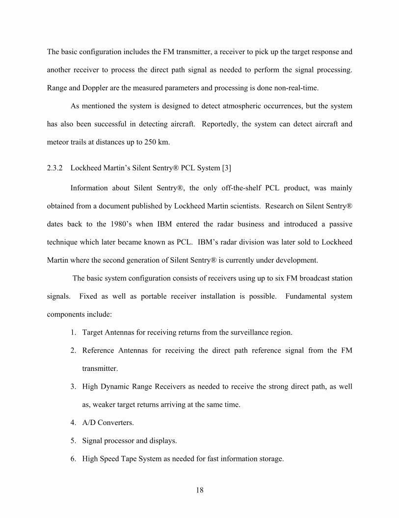
The basic system configuration consists of receivers using up to six FM broadcast station

signals. Fixed as well as portable receiver installation is possible. Fundamental system

components include:

1. Target Antennas for receiving returns from the surveillance region.

2. Reference Antennas for receiving the direct path reference signal from the FM

transmitter.

3. High Dynamic Range Receivers as needed to receive the strong direct path, as well

as, weaker target returns arriving at the same time.

4. A/D Converters.

5. Signal processor and displays.

6. High Speed Tape System as needed for fast information storage.

19

The system is able to effectively track targets, even when only one illuminator

illuminates the target, in which case tracking is two-dimensional and not very accurate. Tracking

quality increasing with more FM transmitters illuminating the target, which leads to three-

dimensional tracking using three and more illuminators.

Mission planning tools are included in the system to enable deployment or performance

simulations around the world. Advertised system performance includes a detection range up to

220 km and a target capacity of 200 flying objects, including everything from aircraft to ballistic

missiles. The system is under continual development. One future capability may include the

incorporation of TV signals not limited by the analog format.

2.3.3 TV Based Bistatic Radar [7,8]

The initial TV based PCL approach of Griffiths and Long failed to provide effective

performance. Since that time, there have been other attempts to use Direct Broadcast Satellite

(DBS) television transmissions for range measurement using TDOA techniques [16]. One

successful technique used analog TV waveforms for target detection and tracking and was

introduced by Howland in the late 1990’s.

Instead of using range measurements, Howland relied on Doppler and bearing

measurements. He used a technique borrowed from the world of sonar, i.e., target location is

determined by measuring both Doppler and bearing of a radiating source [17]. His algorithm

assumes linear, constant velocity target movement during the time interval when location is

estimated. Under this assumption, a given Doppler and bearing history of a target uniquely

defines its location.

The signal processing in Howland’s system begins with spectral analysis of received

signal, where targets are resolved in Doppler. This is followed by a time Constant False Alarm

20

Rate (CFAR) detection scheme for detecting targets. This provides an indication of the target’s

presence and the respective Doppler measurement. Target Direction of Arrival (DOA)

measurements are made through interferometry using two Yagi antennas at the receiver. A 4-by-

4, 16-element planar array to provide improved performance is under development. A Kalman

filter is used to associate target Doppler and DOA measurements. The association of a target’s

Doppler with its DOA information is important for subsequent target parametric estimation.

Doppler and bearing profiles belonging to each target, as provided from the association of

measurements, are used in an extended Kalman filter to estimate Cartesian coordinates and

velocity of each target. Filter initialization is done using a Genetic Algorithm and a Levenberg-

Marquardt optimizer.

Given maximum detection and tracking range is approximately 260 km, the problem

Howland encountered in his experiments is based on the fact that, even target detection was

almost complete, the system could only track one third of the detections. The problem is mainly

attributed to the low information content of the received target response.

2.3.4 Other PCL Concepts

Clearly, most PCL related work has been done in the analog signals field. However, there

are some research efforts using complex structured digital signals as PCL waveforms of

opportunity, including cellular phone signals and digital audio and TV broadcasts [18,19].

In open literature, one can find some resources on the exploitation of digital broadcast

waveforms such as the Digital Audio Broadcast (DAB) waveform. This waveform, with its

relatively wide bandwidth of about 1.5 MHz, offers high resolution in range measurements

through correlation of the received signal with a reference, as done in a matched filtering

process. In the DAB standard a “Coded Orthogonal Frequency Division Multiplexing”

21

(COFDM) technique is used as a multiplexing scheme, which provides excellent multipath

resistance. Experiments using the DAB waveform as a PCL waveform show promising results

[18,19].

In theoretical and practical experiments using the DAB waveform, it has been found that

severe interference from the direct signal (a signal arriving at the receiver along a line-of-sight

path) and clutter affect DAB performance as a radar waveform. For a successful detection

scheme via matched filtering, the direct signal component received in the receiver target channel

should be eliminated or significantly attenuated. The direct signal should be reduced at least 50

dB for a target return 100 dB below the direct signal level to be detected via matched filtering at

the receiver. The reduction is also needed to ensure a reasonable dynamic range of the receiver

[19].

At the same time, there is a strong multipath component in the received waveform that is

mainly attributable to multiple transmitters using the same waveform as done in the “Single

Frequency Network” (SFN) structure supported by DAB signals.

There has been some effort put into removing the direct signal component from the

receiver target channel. There may have been some unofficial successful results; but, no

approach has been publicly discussed in open literature. For this research, a time domain filtering

technique based on signal projection spaces is proposed for removing the direct signal

component from the target channel of the PCL receiver. For this implementation, it is important

to understand the basics of the DAB waveform and the COFDM technique. The next section

provides relevant information on the important aspects of those two concepts.

22

2.4 Digital Audio Broadcast (DAB) waveform

The digital audio technology enabling CD quality sound was first developed for satellite

delivery in the early 1980s. The system operated in 10-12 GHz frequency region and was not

suitable for mobile reception. In addition, “local services”, an important concept of FM

broadcasting, was not possible via satellite delivery and terrestrial digital radio broadcasting

emerged as an alternative. After deciding that earth-based transmission was the best approach,

choosing the right modulation scheme and the right frequency interval became an issue. Initial

work on using Pulse Code Modulation (PCM) in the existing FM broadcast frequency band

failed due to interference and spectral inefficiency [13].

After years of research and development, a consortium called Eureka 147 established a

standard for terrestrial digital radio broadcasting called Digital Audio Broadcasting (DAB). The

chosen DAB transmission method was Coded Orthogonal Frequency Division

Multiplex (COFDM). More than 10 years after the first official presentation of DAB at the

World Administrative Radio Conference 1988 (WARC’88), DAB is still in the introduction

phase. There are some countries across Europe with existing DAB transmitters serving the public

but in most places the system is still under test or in the planning phases [13].

The core of the DAB transmission system is COFDM, a multi-carrier signal transmission

technique that uses multiple low data rate subcarriers to transmit high rate data streams. The

next section introduces the COFDM concepts important to understanding this research.

2.4.1 The COFDM Modulation Technique [20]

The COFDM technique is a special application of “Orthogonal Frequency Division

Multiplex” (OFDM) where “Forward Error Correction” (FEC) is used to further reduce the “Bit

Error Rate” (BER) in a digital communication system. OFDM can be viewed as either a

23

modulation or multiplexing technique. The main reason for using OFDM is its robustness

against frequency selective fading or narrowband interference resulting from its multi-carrier

structure. A single faded frequency or interference source at a particular frequency only affects a

few of the multi-carriers, also called “subcarriers” in OFDM.

There are different ways to implement “frequency division multiplexing” (FDM). The

first technique involves dividing the total available channel bandwidth to N non-overlapping

frequency sub-channels. This technique leads to spectral inefficiency; therefore, overlapping of

individual sub-channels is proposed to provide more efficient bandwidth use at the expense of

increasing BER. To increase system spectral efficiency further, while at the same time reducing

BER, cross-talk between the subcarriers is prevented (minimized) by choosing orthogonal

subcarrier frequencies [20].

24

fc

The frequency bin of the subcarrier with fc as center frequency

. . . . . . . . . . . .

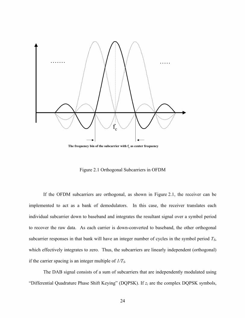
Figure 2.1 Orthogonal Subcarriers in OFDM

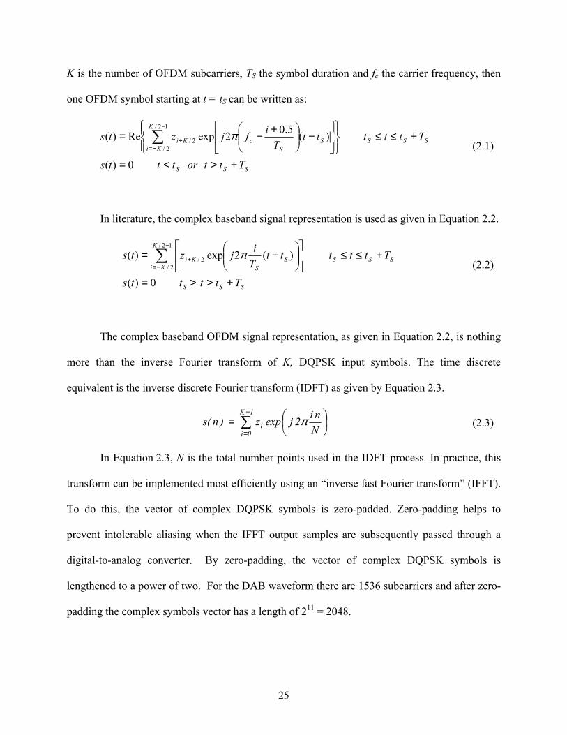
If the OFDM subcarriers are orthogonal, as shown in Figure 2.1, the receiver can be

implemented to act as a bank of demodulators. In this case, the receiver translates each

individual subcarrier down to baseband and integrates the resultant signal over a symbol period

to recover the raw data. As each carrier is down-converted to baseband, the other orthogonal

subcarrier responses in that bank will have an integer number of cycles in the symbol period TS,

which effectively integrates to zero. Thus, the subcarriers are linearly independent (orthogonal)

if the carrier spacing is an integer multiple of 1/TS.

The DAB signal consists of a sum of subcarriers that are independently modulated using

“Differential Quadrature Phase Shift Keying” (DQPSK). If zi are the complex DQPSK symbols,

25

K is the number of OFDM subcarriers, TS the symbol duration and fc the carrier frequency, then

one OFDM symbol starting at t = tS can be written as:

SSS

SSS

K

KiS

ScKi

Tttorttts

TtttttT

ifjzts

+><=

+≤≤

−

+−= ∑−

−=+

0)(

)(5.02expRe)(12/

2/2/ π

(2.1)

In literature, the complex baseband signal representation is used as given in Equation 2.2.

SSS

SSS

K

KiS

SKi

Ttttts

TtttttTijzts

+>>=

+≤≤

−= ∑

−

−=+

0)(

)(2exp)(12/

2/2/ π

(2.2)

The complex baseband OFDM signal representation, as given in Equation 2.2, is nothing

more than the inverse Fourier transform of K, DQPSK input symbols. The time discrete

equivalent is the inverse discrete Fourier transform (IDFT) as given by Equation 2.3.

∑−

=

=

1K

0ii N

ni2jexpz)n(s π (2.3)

In Equation 2.3, N is the total number points used in the IDFT process. In practice, this

transform can be implemented most efficiently using an “inverse fast Fourier transform” (IFFT).

To do this, the vector of complex DQPSK symbols is zero-padded. Zero-padding helps to

prevent intolerable aliasing when the IFFT output samples are subsequently passed through a

digital-to-analog converter. By zero-padding, the vector of complex DQPSK symbols is

lengthened to a power of two. For the DAB waveform there are 1536 subcarriers and after zero-

padding the complex symbols vector has a length of 211 = 2048.

26

Still, the IFFT output is not ready to transmit. To eliminate “intersymbol interference”

(ISI) in the system, a guard time is introduced into each OFDM symbol. Here, a symbol is

defined as the IFFT output or the sum of all DQPSK data modulated subcarriers. The guard

interval is chosen to be larger than the expected delay spread, such that multipath components

from one symbol cannot interfere with the next symbol.

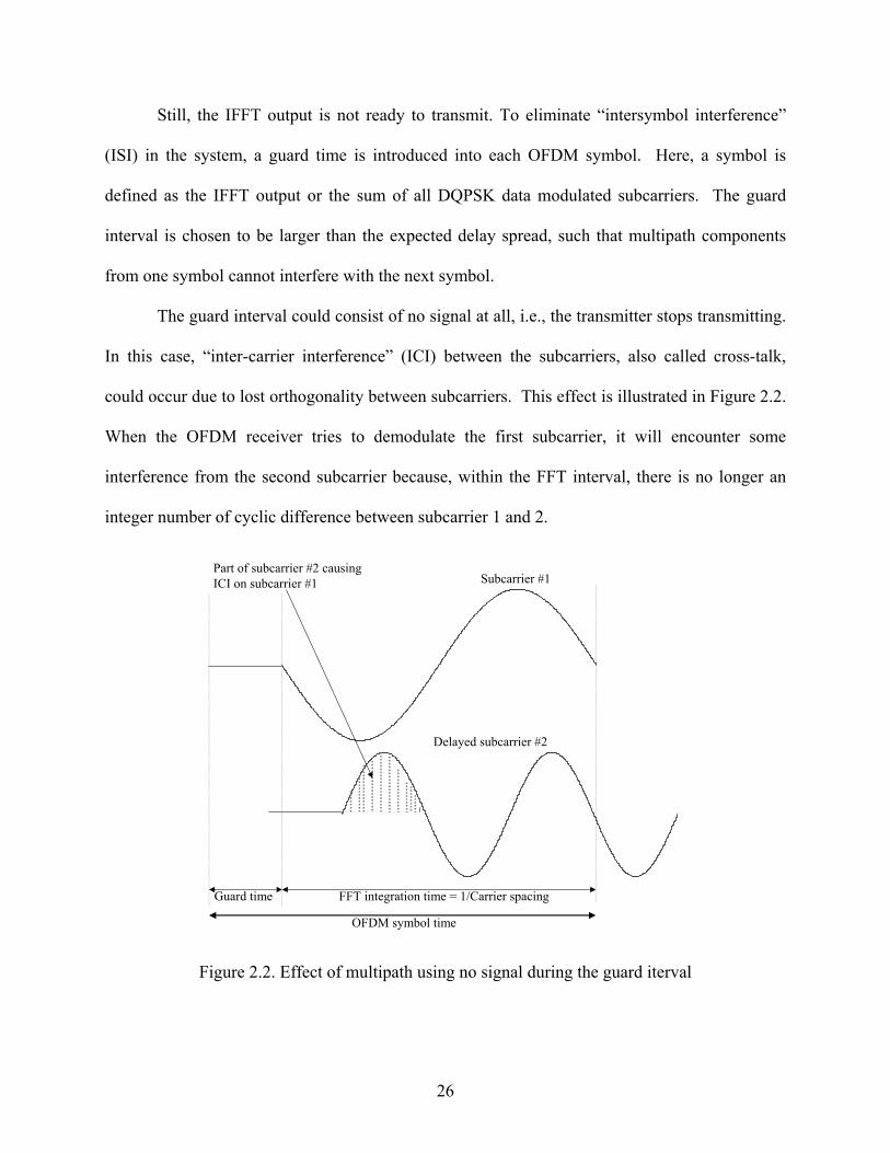
The guard interval could consist of no signal at all, i.e., the transmitter stops transmitting.

In this case, “inter-carrier interference” (ICI) between the subcarriers, also called cross-talk,

could occur due to lost orthogonality between subcarriers. This effect is illustrated in Figure 2.2.

When the OFDM receiver tries to demodulate the first subcarrier, it will encounter some

interference from the second subcarrier because, within the FFT interval, there is no longer an

integer number of cyclic difference between subcarrier 1 and 2.

Subcarrier #1

Delayed subcarrier #2

Guard time FFT integration time = 1/Carrier spacing

OFDM symbol time

Part of subcarrier #2 causingICI on subcarrier #1

Figure 2.2. Effect of multipath using no signal during the guard iterval

27

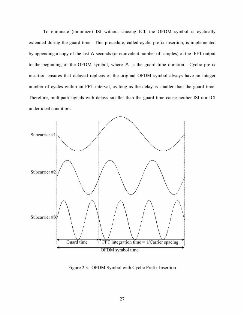
To eliminate (minimize) ISI without causing ICI, the OFDM symbol is cyclically

extended during the guard time. This procedure, called cyclic prefix insertion, is implemented

by appending a copy of the last ∆ seconds (or equivalent number of samples) of the IFFT output

to the beginning of the OFDM symbol, where ∆ is the guard time duration. Cyclic prefix

insertion ensures that delayed replicas of the original OFDM symbol always have an integer

number of cycles within an FFT interval, as long as the delay is smaller than the guard time.

Therefore, multipath signals with delays smaller than the guard time cause neither ISI nor ICI

under ideal conditions.

Guard time FFT integration time = 1/Carrier spacing

OFDM symbol time

Subcarrier #1

Subcarrier #2

Subcarrier #X

Figure 2.3. OFDM Symbol with Cyclic Prefix Insertion

28

The importance of cyclic prefix insertion and the guard interval becomes more evident in

looking at the DAB transmission characteristics. The DAB standard is built around a Single

Frequency Network (SFN) architecture. In a SFN transmitters in a given region transmit the

same signal over a specified channel, hence, multiple, time-delayed copies of the same signal are

simultaneously received which may be correctly called multipath. These multipath signals do

not cause ISI if they arrive at the receiver with a delay no longer than the guard interval.

Therefore, the guard interval duration has an immediate influence on the type of SFN that can be

supported. The longer the guard interval, the greater the maximum allowable distance between

SFN transmitters becomes. However, the signal energy transmitted during the guard interval

(cyclic prefix) is not used by the receiver for data demodulation. Therefore, using a guard

interval actually decreases the channel capacity. Typically, the guard interval is chosen to be no

greater than 4/ST [21]. For DAB Mode I [14], the symbol duration is 1.0 ms and the guard

interval is chosen to be 0.246 ms.

2.4.2 The DAB standard

The DAB signal structure was standardized by ETSI. Details of the standard can be found

in ETS 300 401, a document published by ETSI about DAB related issues. In this section, the

DAB signal structure is given as stated in ETS 300 401:

−−−−= ∑ ∑ ∑∞+

∞−= = −=m

L

l

K

KkSNULLFlkklm

tfj TlTmTtxgzets c

0

2/

2/,,,

2 ))1((Re)( π (2.4)

=

==

− L...,,2,1lfor)T/t(Rect.e

0lfor0)t(g

ST/)t(kj2l,k

U∆π (2.5)

∆+= US TT (2.6)

Various DAB signal parameters and variables are defined as follows:

29

L the number of OFDM symbols per transmission frame (excluding the Null

symbol);

K the number of transmitted subcarriers;

FT the transmission frame duration;

NULLT the Null symbol duration;

ST the duration of OFDM symbol of indices Ll ,...,3,2,1= ;

UT the inverse of the subcarrier frequency spacing;

∆ the duration of the guard interval;

klmz ,, the complex DQPSK symbol associated with carrier k of the OFDM symbol l

during transmission frame m . Its values are defined in the following sub-cases.

For ,0,0 ,, == klmzk so that the central carrier is not transmitted;

cf the central frequency of the signal. [14]

The DAB Mode I transmission frame, as used in this research analyses, includes a total of

77 symbols. The first symbol is the “Null Symbol”. During transmission of the null symbol, the

composite signal )(ts equals zero. The Null symbol and the following “Phase Reference

Symbol” together represent what is called the Synchronization Symbol and are used by the

receivers to synchronize to each transmission frame. Each DAB communication symbol consists

of 1536 subcarriers and is 1.246 ms long, including a cyclic prefix of 0.246 ms. Only the null

symbol has a duration of 1.297 ms.

The phase reference symbol is not only used as part of the synchronization process but

also as a reference for differential data modulation. The phase reference symbol is defined by the

values of klz , for l being the phase reference symbol index.

30

=

<<<<−=

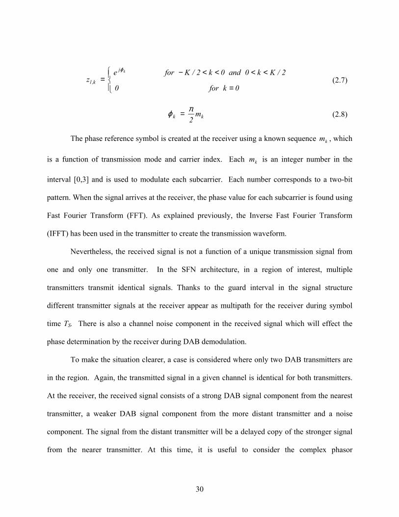
0kfor0

2/Kk0and0k2/Kforez

kj

k,l

ϕ

(2.7)

kk m2πϕ = (2.8)

The phase reference symbol is created at the receiver using a known sequence km , which

is a function of transmission mode and carrier index. Each km is an integer number in the

interval [0,3] and is used to modulate each subcarrier. Each number corresponds to a two-bit

pattern. When the signal arrives at the receiver, the phase value for each subcarrier is found using

Fast Fourier Transform (FFT). As explained previously, the Inverse Fast Fourier Transform

(IFFT) has been used in the transmitter to create the transmission waveform.

Nevertheless, the received signal is not a function of a unique transmission signal from

one and only one transmitter. In the SFN architecture, in a region of interest, multiple

transmitters transmit identical signals. Thanks to the guard interval in the signal structure

different transmitter signals at the receiver appear as multipath for the receiver during symbol

time TS. There is also a channel noise component in the received signal which will effect the

phase determination by the receiver during DAB demodulation.

To make the situation clearer, a case is considered where only two DAB transmitters are

in the region. Again, the transmitted signal in a given channel is identical for both transmitters.

At the receiver, the received signal consists of a strong DAB signal component from the nearest

transmitter, a weaker DAB signal component from the more distant transmitter and a noise

component. The signal from the distant transmitter will be a delayed copy of the stronger signal

from the nearer transmitter. At this time, it is useful to consider the complex phasor

31

representation of individual subcarriers. Specifically, in the transmitter every subcarrier phase is

changed according to the information bits and each subcarrier may be represented by a complex

phasor having the proper phase as a result of DQPSK data modulation. In the receiver, for a

given signal component, the received phase of the complex phasor for each subcarrier is a

function of the transmission phase, subcarrier wavelength and propagation distance (delay time)

from the transmitter to the receiver.

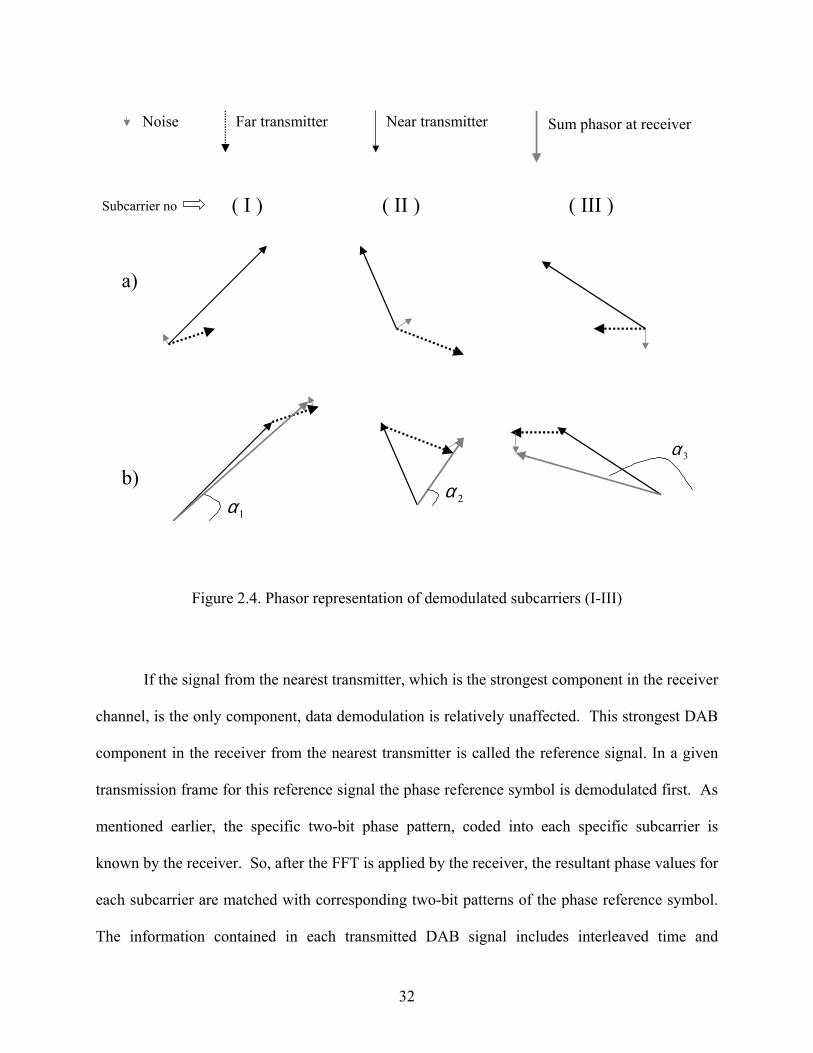
In demodulation at the receiver, the signal is taken to baseband and Fourier transformed,

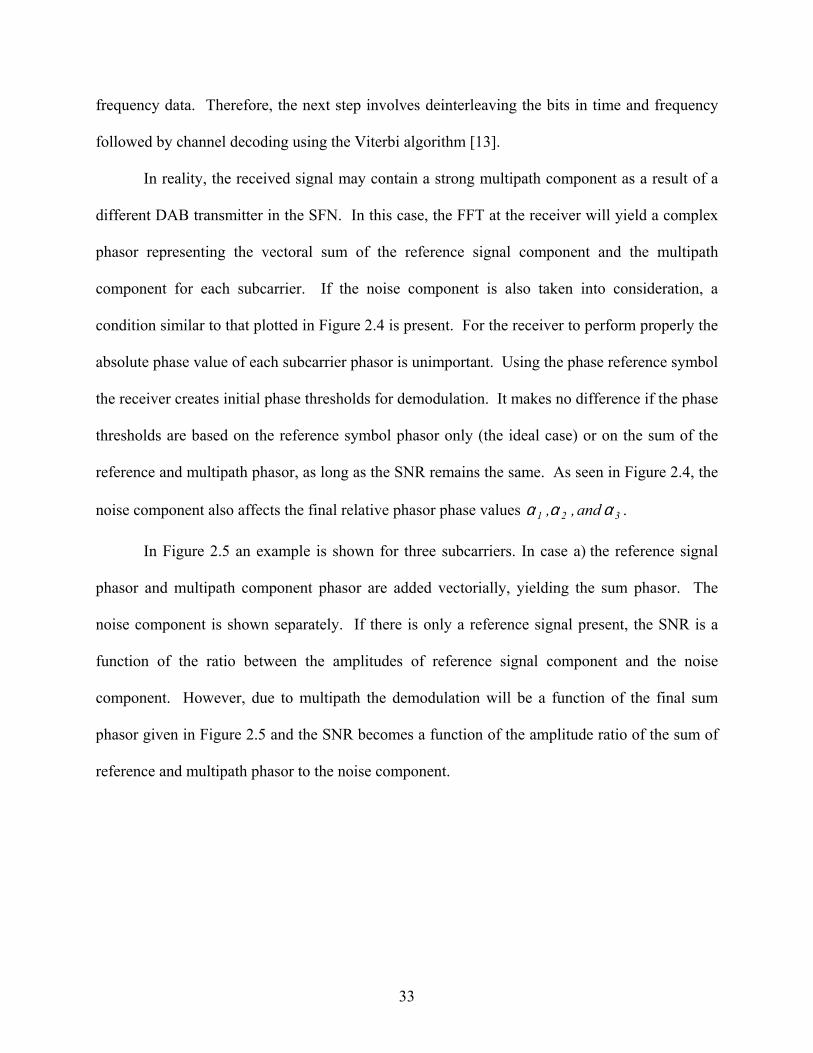
yielding the complex amplitudes for each subcarrier. In Figure 2.4 two cases are indicated. In

case a) the phasor representation for individual components of three subcarriers are given and in

case b) the sum phasor as a result of the FFT at the receiver is given. The resultant phasor for a

given subcarrier after FFT is the vectoral sum of each component shown in case a).

32

Noise Far transmitter Near transmitter Sum phasor at receiver

a)

b)1α 2α

3α

( I ) ( II ) ( III )Subcarrier no

Figure 2.4. Phasor representation of demodulated subcarriers (I-III)

If the signal from the nearest transmitter, which is the strongest component in the receiver

channel, is the only component, data demodulation is relatively unaffected. This strongest DAB

component in the receiver from the nearest transmitter is called the reference signal. In a given

transmission frame for this reference signal the phase reference symbol is demodulated first. As

mentioned earlier, the specific two-bit phase pattern, coded into each specific subcarrier is

known by the receiver. So, after the FFT is applied by the receiver, the resultant phase values for

each subcarrier are matched with corresponding two-bit patterns of the phase reference symbol.

The information contained in each transmitted DAB signal includes interleaved time and

33

frequency data. Therefore, the next step involves deinterleaving the bits in time and frequency

followed by channel decoding using the Viterbi algorithm [13].

In reality, the received signal may contain a strong multipath component as a result of a

different DAB transmitter in the SFN. In this case, the FFT at the receiver will yield a complex

phasor representing the vectoral sum of the reference signal component and the multipath

component for each subcarrier. If the noise component is also taken into consideration, a

condition similar to that plotted in Figure 2.4 is present. For the receiver to perform properly the

absolute phase value of each subcarrier phasor is unimportant. Using the phase reference symbol

the receiver creates initial phase thresholds for demodulation. It makes no difference if the phase

thresholds are based on the reference symbol phasor only (the ideal case) or on the sum of the

reference and multipath phasor, as long as the SNR remains the same. As seen in Figure 2.4, the

noise component also affects the final relative phasor phase values 321 and ,, ααα .

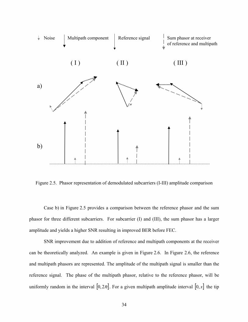
In Figure 2.5 an example is shown for three subcarriers. In case a) the reference signal

phasor and multipath component phasor are added vectorially, yielding the sum phasor. The

noise component is shown separately. If there is only a reference signal present, the SNR is a

function of the ratio between the amplitudes of reference signal component and the noise

component. However, due to multipath the demodulation will be a function of the final sum

phasor given in Figure 2.5 and the SNR becomes a function of the amplitude ratio of the sum of

reference and multipath phasor to the noise component.

34

Noise Multipath component Reference signal Sum phasor at receiver of reference and multipath

a)

b)

( I ) ( II ) ( III )

Figure 2.5. Phasor representation of demodulated subcarriers (I-III) amplitude comparison

Case b) in Figure 2.5 provides a comparison between the reference phasor and the sum

phasor for three different subcarriers. For subcarrier (I) and (III), the sum phasor has a larger

amplitude and yields a higher SNR resulting in improved BER before FEC.

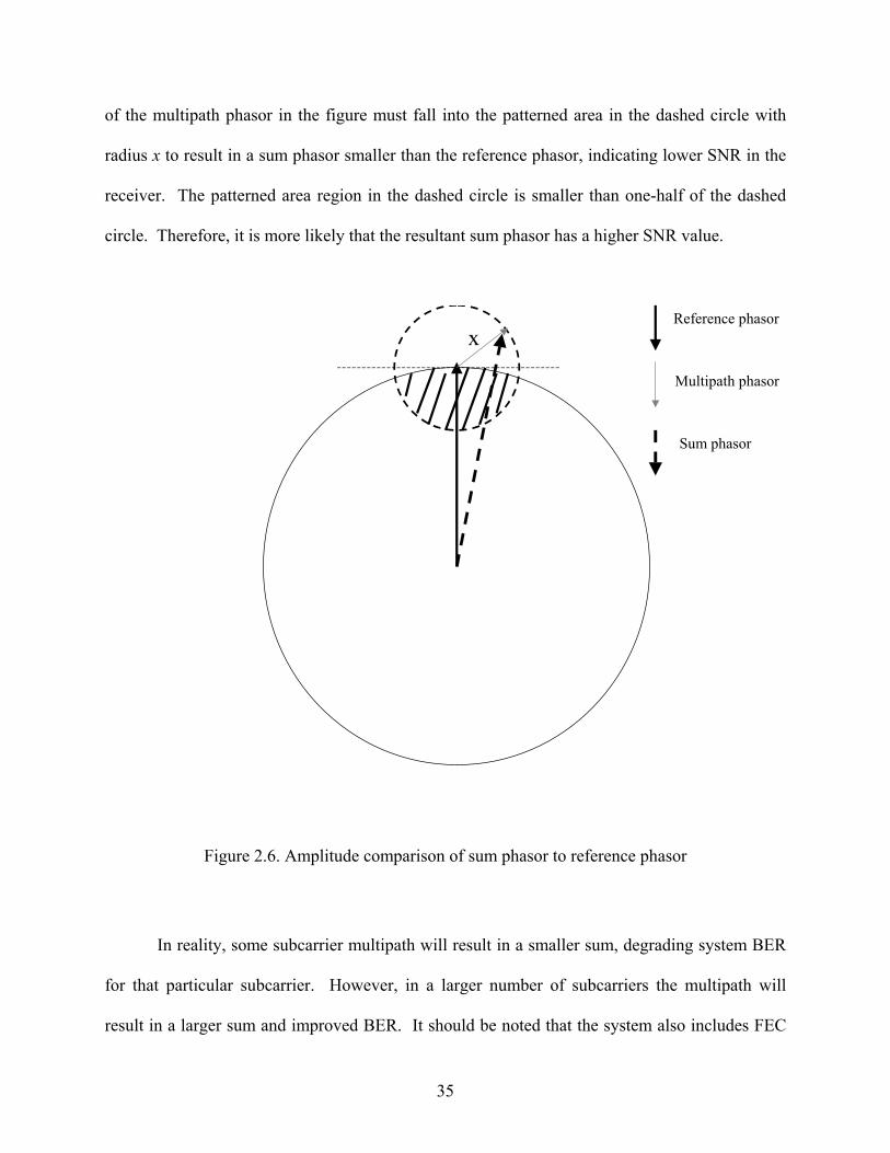
SNR improvement due to addition of reference and multipath components at the receiver

can be theoretically analyzed. An example is given in Figure 2.6. In Figure 2.6, the reference

and multipath phasors are represented. The amplitude of the multipath signal is smaller than the

reference signal. The phase of the multipath phasor, relative to the reference phasor, will be

uniformly random in the interval [ ]π2,0 . For a given multipath amplitude interval [ ]x,0 the tip

35

of the multipath phasor in the figure must fall into the patterned area in the dashed circle with

radius x to result in a sum phasor smaller than the reference phasor, indicating lower SNR in the

receiver. The patterned area region in the dashed circle is smaller than one-half of the dashed

circle. Therefore, it is more likely that the resultant sum phasor has a higher SNR value.

Reference phasor

Multipath phasor

x

Sum phasor

Figure 2.6. Amplitude comparison of sum phasor to reference phasor

In reality, some subcarrier multipath will result in a smaller sum, degrading system BER

for that particular subcarrier. However, in a larger number of subcarriers the multipath will

result in a larger sum and improved BER. It should be noted that the system also includes FEC

36

on time and frequency interleaved bits. Therefore, it can be concluded that multipath signals at

the receiver, as caused by SFN transmission, improves overall DAB receiver performance

provided the multipath delay is less than the guard interval of the system.

2.5 Summary

In this chapter, background material on PCL systems is presented. Different PCL

systems operating with different waveforms of opportunity are introduced. It has been noted that

current systems mainly exploit analog waveforms such as FM radio broadcasts and analog TV

signals. The advantages of using low frequency modulation schemes like FM are stated.

In addition to analog waveforms, newer, more complex waveforms having digital

modulation are also considered for PCL applications. Among these, the Digital Audio Broadcast

(DAB) waveform shows promising results. A closer look at the modulation and multiplexing

scheme of the DAB architecture is shown. It has been found and shown that the modulation as

well as the multiplexing scheme does support possible PCL exploitation of the waveform.

In the next chapter, a filter design is proposed to eliminate the reference signal

component in the PCL receiver target channel. In addition, the ambiguity function is explored as

a means of analyzing the performance of the DAB signal as a PCL waveform. Originating from

the ambiguity function, an analytical tool called a detection surface is introduced to evaluate the

filter performance.

37

CHAPTER 3

METHODOLOGY

3.1 Introduction

In this chapter, the tools required for analyzing the Digital Audio Broadcast (DAB)

waveform for PCL applications are introduced. The discussion starts with a thorough

explanation of the ambiguity function, a powerful analysis tool used to study radar waveform

properties. Next, issues related to the DAB waveform ambiguity function are stated.

Afterwards, a time domain filter design is introduced as a means to enable time difference of

arrival (TDOA) analysis of the DAB signal in a PCL system. The chapter concludes with an

explanation of the signal processing steps taken to implement filtering using MATLAB®.

3.2 Ambiguity Function Analysis [12]

“The ability of a radar to detect targets amongst returns from other objects (clutter) in a

region of interest and the ability to determine parameters of these targets, such as range, bearing,

size and velocity, depends largely on the radar waveform” [11].

For PCL applications using waveforms of opportunity, one does not have the ability to

synthesize optimal waveforms. The approach is to use commercial communication and other

broadcasted waveforms, already present in the environment, as radar waveforms for detecting,

tracking and possibly identifying targets. These commercial signals occupy a certain spectral

region and have distinct modulation characteristics associated with them. Unless a radar

waveform is specifically designed to work for communication and/or broadcasting purposes one

is not able to use a radar-optimized signal in PCL applications. In determining the extent to

38

which a waveform of opportunity can be exploited for radar implementation, the ambiguity

function and resultant ambiguity surface plot provide a useful tool for analysis.

The ambiguity function surface plot and corresponding calculations can be used to

qualitatively assess ‘how well’ a particular waveform achieves and affects:

1. Target detection,

2. Parametric measurement accuracy,

3. Range and Doppler resolution,

4. Ambiguities, and

5. Clutter rejection.

The ambiguity function is widely used as a tool for analyzing radar waveform

performance [12]. Basically, it is a series of correlation integrals, or the absolute value squared,

based on matched filter detection, where a received signal having different Doppler shifts and

time delays is correlated with a reference signal containing no Doppler shift or time delay. To

understand the ambiguity function it is useful to start by introducing the output of the matched

filter as:

dtTtstsr RrMF )(*)( '∫ −= (3.1)

In Equation 3.1, )(tsr is the “received signal”, )(ts is the transmitted or “reference

signal”, )(* ts is the complex conjugate of the reference signal, and 'RT is the estimated time

delay. Using complex signal representations, the transmitted signal can be written as

]2exp[|)(| tfjtu oπ , where )(tu is the “complex modulation function” whose magnitude is the

envelope of the real signal, and 0f is the carrier frequency. The received signal )(tsr is

assumed equal to the transmitted signal except for a Doppler shift of df and a time delay

39

equaling the true time delay oT . Therefore, the matched filter response of Equation 3.1

becomes:

dtTtfjTtffjTtuTtus RdRMF )](2exp[)])((2exp[)(*)( '000

'0 −−−+−−= ∫ ππ (3.2)

For simplicity in understanding this equation, the origin of the ambiguity surface is taken

to be the true time delay and transmitted frequency, i.e., 0,0 00 == fT and RRR TTTT =−=− ''0 .

After some simplifications, the matched filter output becomes:

∫ +=T

dRdR dttfjTtutufT0

)2exp()(*)(),( πχ (3.3)

Here, | ),( dR fTχ |2 will be called the ambiguity function. Properties of the ambiguity

function include:

1. The maximum value of the ambiguity function occurs at the origin as expressed by

Equation 3.4. This occurs since the received signal arrives at the receiver with the same

time delay and zero Doppler shift as the reference waveform; this is effectively the basic

auto-correlation response of the waveform.

Maximum Value: 222max )2()0,0(||),(| EfT dR == χχ (3.4)

40

2. As expressed by Equation 3.5, the ambiguity surface, created by plotting the

ambiguity function as a function of time delay RT and Doppler df , is symmetric along

both the time delay and frequency axes.

Symmetry Relation: 22 |),(||),(| dRdR fTfT χχ =−− (3.5)

3. The total volume under the ambiguity surface is constant and equals (2E)2 per

Equation 3.6.

Volume Under Surface: 22 )2(|),(| EdfdTfT dRdR =∫∫ χ (3.6)

The maximum value property of Equation 3.4 states that the value at the origin of the

ambiguity function is 2)2( E , where E is the total Energy contained in the signal. Likewise,

Equation 3.6 indicates that the total volume under the ambiguity surface is also 2)2( E . This is a

total volume constraint that may be satisfied by many different surfaces as determined by the

waveform; whereas, the maximum value is finite at the origin.

There are specific methods for calculating the ambiguity function. The first technique

considered multiplies u(t) with u(t+TR) and then uses an Inverse Fast Fourier Transform (IFFT)

to calculate Equation 3.3. The complex exponential representation of the signal, as used in this

equation, is the reason why IFFT techniques can be used.

In the second technique, for a given frequency Doppler shift df , the term

)2exp()(* tfjtu dπ is first calculated. Then, )(tu is correlated with )2exp()(* tfjtu dπ . The

correlator output for different df values yields the ambiguity function of Equation 3.3.

Correlation in the time domain corresponds to multiplication in the frequency domain, i.e., the

41

Fourier spectrum of the resultant ambiguity function can be obtained through multiplication of

the Fourier transforms of )(tu and )2exp()(* tfjtu dπ . Therefore, one specific implementation

of the second technique involves calculating the Fourier transforms of )(tu and

)2exp()(* tfjtu dπ for different df values first. Then, the frequency domain transforms are

multiplied and the result is the Fourier transform of the ambiguity function. Hence, by taking the

IFFT of the result the desired response of Equation 3.3 is obtained. If implemented for every

Doppler shift df , the ambiguity surface can be created as in Figure 3.1. This method is

employed for this research.

Time axis

Frequency axis

Nor

mal

ized

Am

bigu

ity fu

nctio

n

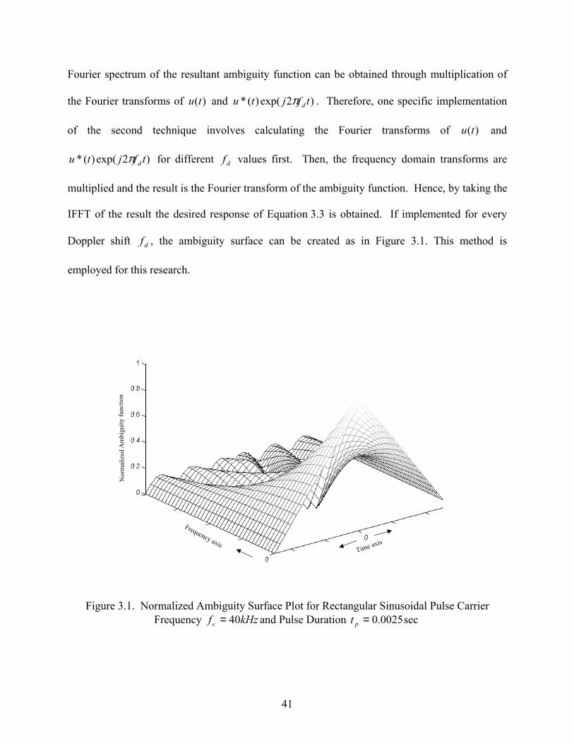
Figure 3.1. Normalized Ambiguity Surface Plot for Rectangular Sinusoidal Pulse Carrier

Frequency kHzfc 40= and Pulse Duration sec0025.0=pt

42

Under ideal conditions, the ambiguity surface consists of a single peak having

infinitesimal thickness at the origin and zero elsewhere, i.e., an impulse function having no

ambiguities in range or Doppler. However, because of ambiguity function properties and the

resulting surface plot it is not possible to achieve the ideal impulse function at the origin. The

peak width along the time delay axis determines the accuracy and resolution of time domain

measurements, e.g., target range; and, the width along the Doppler axis determines the

achievable accuracy and resolution in frequency domain measurements, e.g., velocity. In both

domains a smaller peak width results in better resolution performance. Also, the higher the peak

value at the origin, relative to the surrounding values, the better the measurement accuracy

becomes.

There is a lot to learn by analyzing the ambiguity surface of simple waveforms that one

can carry into analyzing more complex waveforms. By examining the rectangular sinusoidal

pulse ambiguity surface of Figure 3.1 one sees a triangle-shaped response of the ambiguity

function along the time axis where there is no Doppler shift. This response is shown in

Equation 3.7, which is the evaluation of Equation 3.3 using a Doppler frequency shift of zero.

∫ +=T

RR dtTtutuT0

)(*)()0,(χ (3.7)

The expression in Equation 3.7 can also be seen as the autocorrelation of complex

function )(tu . The time axis properties of Figure 3.1, along with the calculations from Equation

3.7, yields a metric for evaluating the time domain performance of the waveform, the simple

rectangular sinusoidal pulse in this case. In the context of this research, time domain

43

performance is defined as the achievable measurement accuracy and resolution provided by the

waveform.

Time axis

Frequency axis

Nor

mal

ized

Am

bigu

ity fu

nctio

n

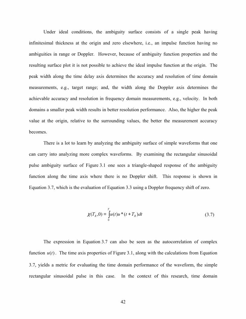
Figure 3.2. Normalized Ambiguity Surface Plot, Rectangular Sinusoidal Pulse Carrier

Frequency kHzfc 40= and Pulse Duration sec005.0=pt .

Figure 3.2 is the ambiguity surface for a longer sinusoidal pulse than used to generate

Figure 3.1, sec005.0=pt versus sec0025.0=pt . The sinusoid amplitudes are equal. The

resultant peak at the origin is wider. In fact, the non-normalized peak response at the origin of

Figure 3.2 is higher than the peak response of the shorter pulse ambiguity surface of Figure 3.1,

as dictated by Equation 3.4. Although target detection capability is a function of the absolute

peak of the ambiguity surface, the measurement accuracy and resolution are not. In fact, time

delay measurement resolution and accuracy is a function of frequency signal bandwidth B.

44

Therefore, for time domain analysis, one can conclude that shorter time sinusoidal pulses provide

better range measurement accuracy and resolution.

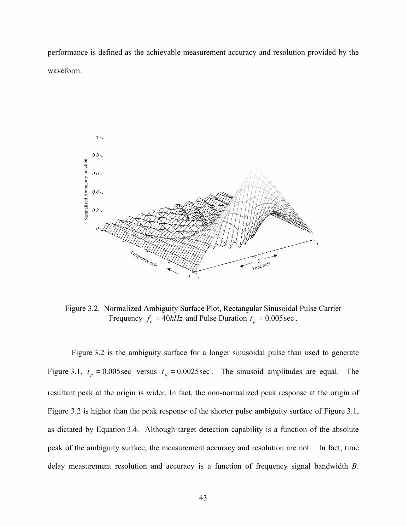
Ambiguity surface analysis of the simple sinusoidal pulse can be continued by analyzing

Equation 3.3 along the frequency axis where time delay is zero. The resultant equation is given

in Equation 3.8 below.

∫=T

dd dttfjtutuf0

)2exp()(*)(),0( πχ (3.8)

Equation 3.8 is constructed much like an IFFT of the product )(*)( tutu . From Fourier

transform theory, this is equivalent to correlation of the IFFT’s of )(tu and )(* tu or the

autocorrelation of the IFFT of )(tu . From duality, the Fourier transform of )(tu , being a

sinusoidal pulse, has a sinc-shaped IFFT. The sinc-shaped IFFT of )(tu is thus correlated with

itself yielding the zero time delay surface cut of the ambiguity surface.

45

0 200 400 600 800 1000 1200 1400 16000

0.1

0.2

0.3

0.4

0.5

0.6

0.7

0.8

0.9

1

Nor

mal

ized

am

bigu

ity fu

nctio

n

Frequencyaxis(Hz)

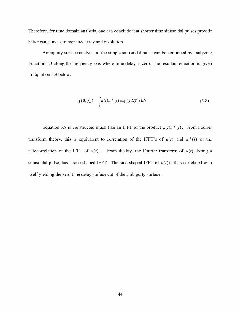
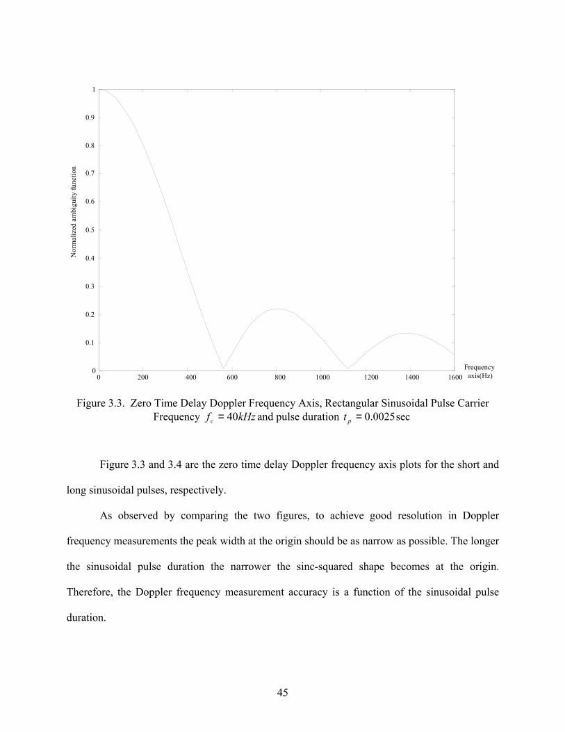
Figure 3.3. Zero Time Delay Doppler Frequency Axis, Rectangular Sinusoidal Pulse Carrier Frequency kHzfc 40= and pulse duration sec0025.0=pt

Figure 3.3 and 3.4 are the zero time delay Doppler frequency axis plots for the short and

long sinusoidal pulses, respectively.

As observed by comparing the two figures, to achieve good resolution in Doppler

frequency measurements the peak width at the origin should be as narrow as possible. The longer

the sinusoidal pulse duration the narrower the sinc-squared shape becomes at the origin.

Therefore, the Doppler frequency measurement accuracy is a function of the sinusoidal pulse

duration.

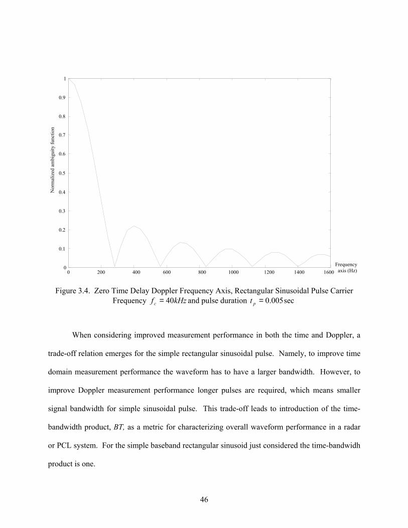
46

0 200 400 600 800 1000 1200 1400 16000

0.1

0.2

0.3

0.4

0.5

0.6

0.7

0.8

0.9

1

Nor

mal

ized

am

bigu

ity fu

nctio

n

Frequencyaxis (Hz)

Figure 3.4. Zero Time Delay Doppler Frequency Axis, Rectangular Sinusoidal Pulse Carrier Frequency kHzfc 40= and pulse duration sec005.0=pt

When considering improved measurement performance in both the time and Doppler, a

trade-off relation emerges for the simple rectangular sinusoidal pulse. Namely, to improve time

domain measurement performance the waveform has to have a larger bandwidth. However, to

improve Doppler measurement performance longer pulses are required, which means smaller

signal bandwidth for simple sinusoidal pulse. This trade-off leads to introduction of the time-

bandwidth product, BT, as a metric for characterizing overall waveform performance in a radar

or PCL system. For the simple baseband rectangular sinusoid just considered the time-bandwidh

product is one.

47

3.3 Ambiguity function analysis of the DAB waveform

The analysis of more complex waveforms is not as straightforward as the simple

sinusoidal pulse case. In case of a DAB the signal consists of multiple symbols transmitted

sequentially. Each symbol consists of several subpulses having pseudo-random DQPSK

modulation that are coherently added and simultaneously transmitted. Details of the DAB

waveform structure are given in Chapter 2. For ambiguity surface analysis of the DAB

waveform the complex )(tu function can be formed using any number of subpulses and DAB

symbols. The total number of DAB symbols used in forming )(tu determines the “coherent

integration time” for calculations in Equation 3.3. Coherent integration time as well as the

number of subcarrier pulses per symbol affects DAB waveform performance in PCL system

applications. The time-bandwidth product of a DAB PCL waveform is generally much higher

than one. In the DAB waveform case the resolution of time delay measurements and frequency

shift measurements can be dealt independently, i.e., both can be improved simultaneously.

Concerning the DAB waveform structure defined as COFDM, simultaneous improvement is

provided by

1. Using more orthogonal-subcarriers per symbol to effectively increase the

signal bandwidth, thereby improving time delay measurement performance,

and

2. Increasing the coherent integration time by increasing number of symbols in

the representative radar waveform, thereby extending the signal time duration

and improving Doppler frequency measurement performance without

degrading time domain performance.

48

Note that increasing the number of symbols per coherent integration time does not affect

the DAB signal bandwidth – DAB signal bandwidth is a function of the number of orthogonal

subcarriers per symbol and the time duration of each symbol.

Two methods for calculating the ambiguity function were introduced earlier. For this

research, the second method has been adopted and implemented per the following (where did

you introduce it)

1. FFTs of )(tu and )2exp()(* tfjtu dπ for the desired df value is computed,

2. The resultant frequency responses are multiplied to produce the frequency domain

representation of the ambiguity function as given by Equation 3.3,

3. An IFFT is taken to yield a range profile (time response) at the selected df value.

This procedure is repeated along the frequency shift axis for different df values to yield

the complete ambiguity function.

For any given signal the ambiguity function provides a measure of correlation between

reference signal )(tu and the Doppler-shifted version of the reference signal expressed as

)2exp()(* tfjtu dπ . In fact, the reference signal itself may be Doppler-shifted as well. In this

case, df axis of the ambiguity surface represents the relative Doppler frequency shift between

the reference )(tu and )2exp()(* tfjtu dπ , which can be thought as the return of the reference

signal from a moving object, called a target.

In general, any waveform used for calculating an ambiguity function perfectly correlates

with itself yielding a maximum function value at zero time delay and Doppler frequency shift.

The correlation output decreases when a time delayed or Doppler shifted version of the reference

is correlated with the reference waveform. This relationship can be used for determining

49

waveform target detection capability through calculation of the ambiguity function and plotting

of the ambiguity surface.

In PCL applications, and radar applications in general, the time-delay and Doppler shift

of a received target return is unknown. Assuming an independent reference signal can be created

at the receiver one simple parametric detection and estimation technique for unknown target

characteristics consists of:

1. Adding a time delay and Doppler shift to the reference waveform,

2. Correlating this waveform with the received target return signal,

3. Repeating steps 1 and 2 until the entire “detection surface” is generated,

4. Locating the peak correlation response on the surface, and

5. Estimating the unknown target parameters as those coinciding with the time delay

(range estimate) and Doppler (relative velocity estimate) values where the peak

occurs.

Theoretically, the highest correlation response occurs when both components entering the

correlation are equal. Another possible outcome is that a peak value is not sufficient to trigger

target detection, e.g., a target response is present but it has insufficient energy to produce a

surface response above the noise floor. Alternately, if a target is not present, the calculated

ambiguity function will always have a peak response somewhere. Whether or not a peak

response corresponds to a target or not is ultimately determined by the signal processing

techniques used. Ambiguity function calculation and ambiguity surface analysis of the reference

waveform response is a vital input for any signal processing effort for detecting targets with a

matched filtering approach. For example, thresholding can utilize a peak to sidelobe ratio of

ambiguity surface.

50

The real utility of the ambiguity surface can be best exploited if the inputs to the

ambiguity function formula of Equation 3.3 are realistic, i.e., when the reference waveform is

being Doppler-shifted, the signal return of the reference waveform from a target with a relative

velocity corresponds to the applied Doppler-shift. This implementation is relatively easy for

simple sinusoidal pulsed waveforms. If the reference waveform consists of more than one

sinusoidal subpulse, as the case in DAB, the situation gets much more complex. Namely, each

subpulse, or DAB subcarrier, experiences a different Doppler frequency shift as dictated by its

carrier frequency (or wavelength) and the relative velocity of a moving target. DAB Mode I has

1536 different subcarrier center frequencies [14]. Therefore, shifting all subcarriers by the same,

constant Doppler frequency is not a realistic approach. However, there is an advantage gained

by applying a constant frequency shift to all subcarriers. Namely, the ambiguity surface

calculations become much faster since a simple IFFT can be used to create the Doppler shifted

signal.

This next section explains how a simple IFFT can be used to create the frequency shifted

DAB waveform (assuming a constant Doppler shift for all subcarriers) as well as an explanation

of the theoretically correct, but more tedious way to calculate the frequency dependent Doppler

shifted DAB signal.

The DAB Mode I waveform consists of 1536 orthogonal subcarriers of 1.246

milliseconds duration transmitted simultaneously as single DAB symbol. As mentioned in

Chapter 2, there is a cyclic prefix added to the beginning of each subcarrier, i.e., 0.246

milliseconds from the end of each subcarrier is copied and pasted at the beginning [14].

Basically, each DAB symbol can be written as the sum of 1536 orthogonal sinusoids as given in

Equation 3.9. Detailed information related to DAB waveform is included in Chapter 2.

51

∑=

+=1536

1)2cos(

iiit tfs θπ (3.9)

Given a DAB signal is transmitted, the return signal from a moving target will induce a

different Doppler frequency shift df on each subcarrier as determined by the subpulse center

frequency if . The target return will be similar to the expression in Equation 3.10:

∑=

++=1536

1]2)cos[(

iidiT tffs

iθπ (3.10)

Equation 3.10 is the proper analytic form of a Doppler shifted DAB symbol, clearly

indicating a subpulse carrier dependent Doppler component. To accurately simulate this Doppler

shifted symbol one has to induce a different Doppler shift on each subcarrier frequency for a

given relative velocity. For computer simulations this approach is impractical. It is desirable to

have a fast algorithm for computing the Doppler shifted DAB signal without losing important

information. One fast approach is to assume a constant Doppler shift (subcarrier frequency

independent) for every subcarrier, thereby, that fast IFFT technique can be used to create target

return signals. To demonstrate this approach, Equation 3.10 is rearranged and rewritten to

include a constant Doppler shift df as illustrated in Equation 3.11. By applying some

trigonometric identities, Equation 3.12 through Equation 3.14 show the fast IFFT creation of a

Doppler shifted DAB signal.

∑=

++=1536

1]2)2cos[(

idiiT tftfs πθπ (3.11)

∑=

+−+=1536

1)2sin()2sin()2cos()2cos(

iiidiidT tftftftfs θππθππ (3.12)

52

∑ ∑= =

+−+=1536

1

1536

1)2sin()2sin()2cos()2cos(

iii

idiidT tftftftfs θππθππ (3.13)

))]((Im[)2sin())]((Re[)2cos( ididT gIFFTtfgIFFTtfs θπθπ −= (3.14)

In going from Equation 3.13 to Equation 3.14, the ∑=

1536

1i)2cos( ii tf θπ + term is replaced

by ))]((Re[ igIFFT θ and the )2sin(1536

1ii

itf θπ +∑

=

term is replaced by ))]((Im[ igIFFT θ . This

IFFT representation was introduced in Chapter 2 to facilitate the efficient creation of DAB

subcarriers. Therefore, under the assumption of constant Doppler shift for all subcarriers, the

IFFT can be used for DAB signal formation and for constructing a Doppler shifted target return.

Clearly, assuming a constant subcarrier Doppler shift produces error. The question is, how much

error is introduced. The amount of error created by this assumption, and its effect on ambiguity

function calculation and surface generation, is demonstrated in Chapter 4.

3.4 Practical issues with DAB-PCL system

This section introduces a detrimental factor present in the implementation of a realistic

PCL system, namely, the presence of a strong reference signal component in the target channel

of a PCL receiver. A PCL receiver dedicated to exploiting DAB waveform may use matched

filter techniques for signal processing and target detection. For this particular processing

technique, at least two receiver channels are necessary. One channel is dedicated to receiving

the reference waveform, defined as the direct response from a line-of-sight (LOS) transmitter.

The second receiver channel called the target channel, i.e., the antenna of this receiver channel is

specifically directed towards a surveillance region to receive target returns (echoes) of the

reference waveform. It is practically impossible to completely isolate the two receiver channels,

53

i.e., one component of the reference channel signal is a weaker target return and one component

of the target channel signal is a stronger reference signal response.

The target return component in the reference channel does not pose a serious problem

since this component is generally very much lower in power. Thus, it does not affect system

performance. However, reference signal leakage into the target channel signal significantly

affects system performance. A rigorous mathematical analysis of this detrimental effect is

provided in reference 11 with important conclusions from this analysis provided below.

Equation 3.15 and Equation 3.16 are the received signals for both channels, including the

interfering components.

)2exp()()()( 1110 tfjttututur παα −+= (3.15)

)2exp()()()( 1110 tfjttututut πββ −+= (3.16)

In Equation 3.15 )(tur is the received signal in the reference channel and contains two

components, reference signal component )(0 tuα and target return component

)2exp()( 111 tfjttu πα − . The target return component is nothing more than the reference signal

delayed in time by 1t (a function of target range) and shifted in frequency by 1f (a function of

target relative velocity). As shown in Equation 3.16, the received signal in the target channel

)(tut contains similar components with different weights of 0β and 1β . If the weights are

compared, one sees that the largest weight is 0α , the weight of the reference component in the

reference channel. Although the target channel is dedicated to receiving and processing the

target return signal and, therefore, it is desirable for the target return component to dominate in

this channel; in practice there is often strong leakage from the LOS transmitter and the reference

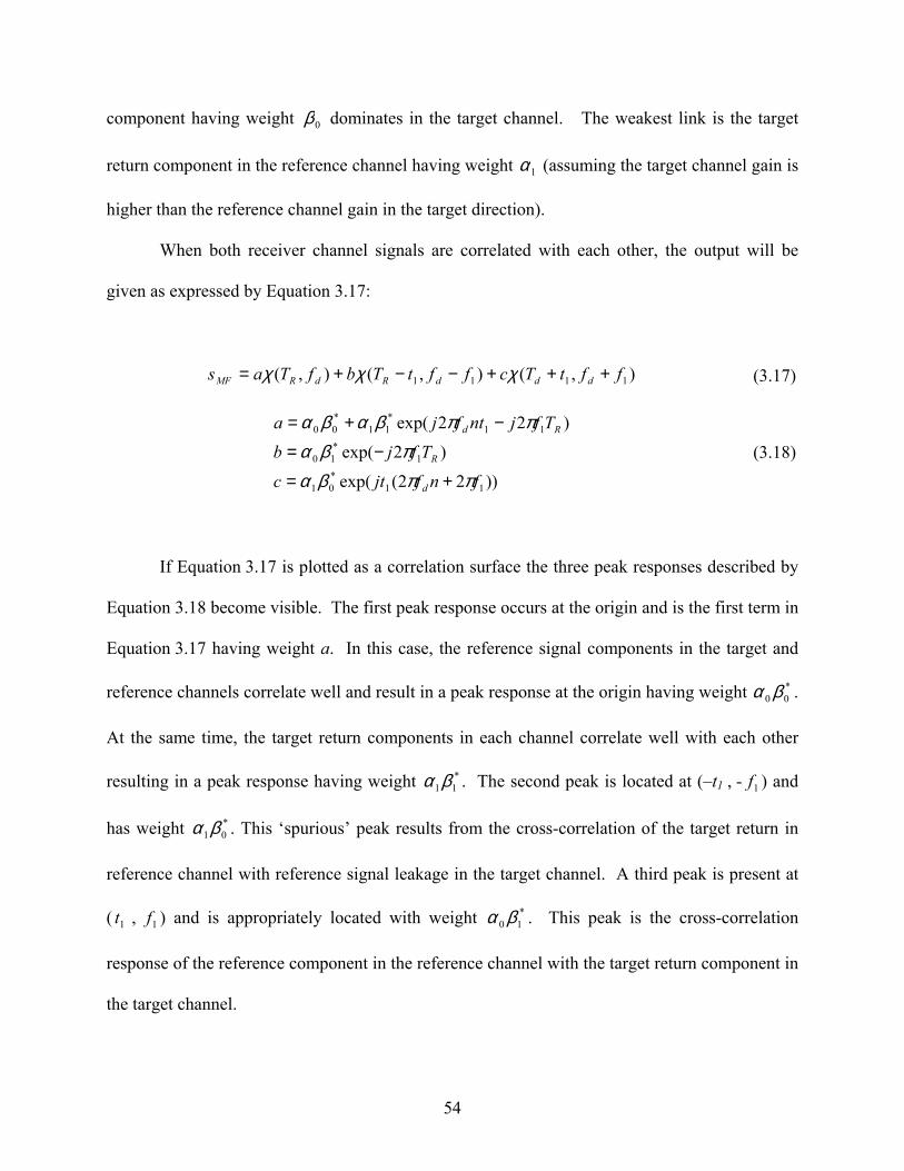
54

component having weight 0β dominates in the target channel. The weakest link is the target

return component in the reference channel having weight 1α (assuming the target channel gain is

higher than the reference channel gain in the target direction).

When both receiver channel signals are correlated with each other, the output will be

given as expressed by Equation 3.17:

),(),(),( 1111 fftTcfftTbfTas dddRdRMF +++−−+= χχχ (3.17)

))22(exp(

)2exp(

)22exp(

11*01

1*10

11*11

*00

fnfjtc

Tfjb

Tfjntfja

d

R

Rd

ππβαπβα

ππβαβα

+=

−=

−+=

(3.18)

If Equation 3.17 is plotted as a correlation surface the three peak responses described by

Equation 3.18 become visible. The first peak response occurs at the origin and is the first term in

Equation 3.17 having weight a. In this case, the reference signal components in the target and

reference channels correlate well and result in a peak response at the origin having weight *00 βα .

At the same time, the target return components in each channel correlate well with each other

resulting in a peak response having weight *11βα . The second peak is located at (–t1 , - 1f ) and

has weight *01βα . This ‘spurious’ peak results from the cross-correlation of the target return in

reference channel with reference signal leakage in the target channel. A third peak is present at

( 1t , 1f ) and is appropriately located with weight *10 βα . This peak is the cross-correlation

response of the reference component in the reference channel with the target return component in

the target channel.

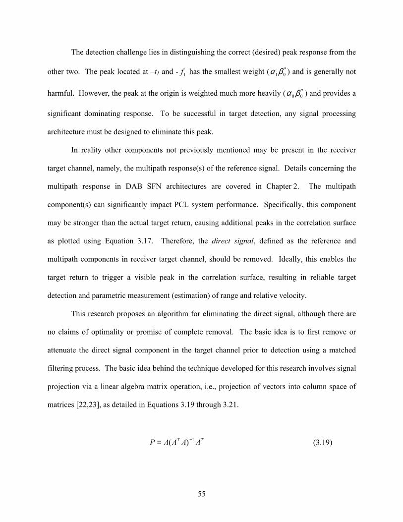
55

The detection challenge lies in distinguishing the correct (desired) peak response from the

other two. The peak located at –t1 and - 1f has the smallest weight ( *01βα ) and is generally not

harmful. However, the peak at the origin is weighted much more heavily ( *00 βα ) and provides a

significant dominating response. To be successful in target detection, any signal processing

architecture must be designed to eliminate this peak.

In reality other components not previously mentioned may be present in the receiver

target channel, namely, the multipath response(s) of the reference signal. Details concerning the

multipath response in DAB SFN architectures are covered in Chapter 2. The multipath

component(s) can significantly impact PCL system performance. Specifically, this component

may be stronger than the actual target return, causing additional peaks in the correlation surface

as plotted using Equation 3.17. Therefore, the direct signal, defined as the reference and

multipath components in receiver target channel, should be removed. Ideally, this enables the

target return to trigger a visible peak in the correlation surface, resulting in reliable target

detection and parametric measurement (estimation) of range and relative velocity.

This research proposes an algorithm for eliminating the direct signal, although there are

no claims of optimality or promise of complete removal. The basic idea is to first remove or

attenuate the direct signal component in the target channel prior to detection using a matched

filtering process. The basic idea behind the technique developed for this research involves signal

projection via a linear algebra matrix operation, i.e., projection of vectors into column space of

matrices [22,23], as detailed in Equations 3.19 through 3.21.

TT AAAAP 1)( −= (3.19)

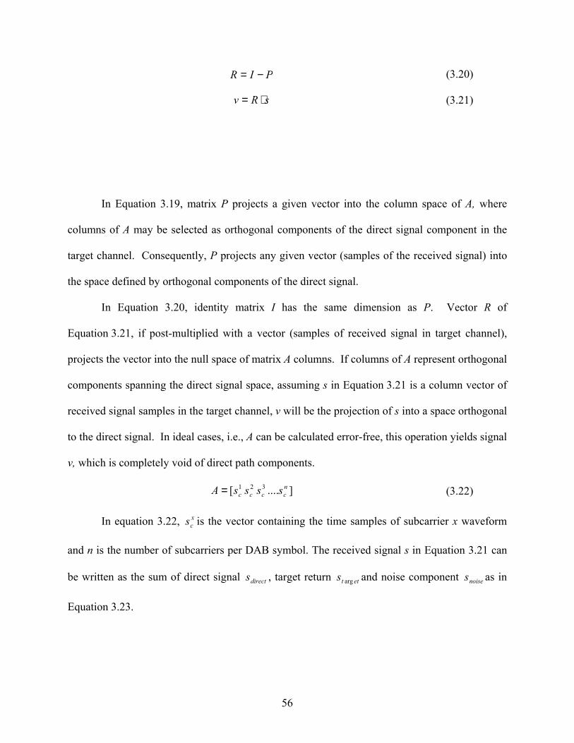
56

PIR −= (3.20)

sRv ⋅= (3.21)

In Equation 3.19, matrix P projects a given vector into the column space of A, where

columns of A may be selected as orthogonal components of the direct signal component in the

target channel. Consequently, P projects any given vector (samples of the received signal) into

the space defined by orthogonal components of the direct signal.

In Equation 3.20, identity matrix I has the same dimension as P. Vector R of

Equation 3.21, if post-multiplied with a vector (samples of received signal in target channel),

projects the vector into the null space of matrix A columns. If columns of A represent orthogonal

components spanning the direct signal space, assuming s in Equation 3.21 is a column vector of

received signal samples in the target channel, v will be the projection of s into a space orthogonal

to the direct signal. In ideal cases, i.e., A can be calculated error-free, this operation yields signal

v, which is completely void of direct path components.

]....[ 321 ncccc ssssA = (3.22)

In equation 3.22, xcs is the vector containing the time samples of subcarrier x waveform

and n is the number of subcarriers per DAB symbol. The received signal s in Equation 3.21 can

be written as the sum of direct signal directs , target return etts arg and noise component noises as in

Equation 3.23.

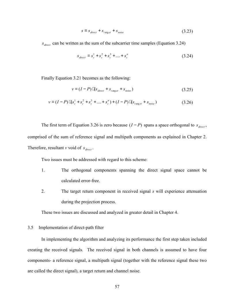
57

noiseettdirect ssss ++= arg (3.23)

directs can be written as the sum of the subcarrier time samples (Equation 3.24)

nccccdirect sssss ++++= ....321 (3.24)

Finally Equation 3.21 becomes as the following:

)()( arg noiseettdirect sssPIv ++⋅−= (3.25)

)()()....()( arg321

noiseettncccc ssPIssssPIv +⋅−+++++⋅−= (3.26)

The first term of Equation 3.26 is zero because )( PI − spans a space orthogonal to directs ,

comprised of the sum of reference signal and multipath components as explained in Chapter 2.

Therefore, resultant v void of directs .

Two issues must be addressed with regard to this scheme:

1. The orthogonal components spanning the direct signal space cannot be

calculated error-free.

2. The target return component in received signal s will experience attenuation

during the projection process.

These two issues are discussed and analyzed in greater detail in Chapter 4.

3.5 Implementation of direct-path filter

In implementing the algorithm and analyzing its performance the first step taken included

creating the received signals. The received signal in both channels is assumed to have four

components- a reference signal, a multipath signal (together with the reference signal these two

are called the direct signal), a target return and channel noise.

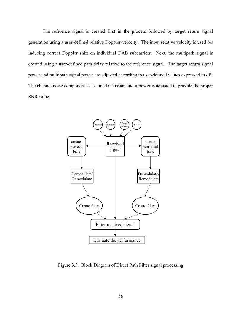
58

The reference signal is created first in the process followed by target return signal

generation using a user-defined relative Doppler-velocity. The input relative velocity is used for

inducing correct Doppler shift on individual DAB subcarriers. Next, the multipath signal is

created using a user-defined path delay relative to the reference signal. The target return signal

power and multipath signal power are adjusted according to user-defined values expressed in dB.

The channel noise component is assumed Gaussian and it power is adjusted to provide the proper

SNR value.

NoiseTargetreturnmultipathreference

Create filter

Filter received signal

Evaluate the performance

Receivedsignal

create perfect

base

createnon-ideal

base

Demodulate/Remodulate

Create filter

Demodulate/Remodulate

Figure 3.5. Block Diagram of Direct Path Filter signal processing

59

As explained in Chapter 2 the DAB signal is transmitted in frames. The first non-zero,

data modulated symbol of every DAB frame transmission is the phase reference symbol. A

phase reference symbol having a predetermined code sequence is known a priori by the receiver

and used to determine subcarrier phase thresholds (this is required for DQPSK demodulation).

This represents an important part of the DAB waveform demodulation process, where indirectly,

the channel frequency response is estimated and used to achieve “near error-free” data

demodulation.

Two different phase reconstruction cases have been simulated for this research. The first

case assumes perfect construction of the phase thresholds for each subcarrier, which requires the

phase reference symbol to be made up of only the direct signal component. In this case, the

received signal can be demodulated correctly. Although in the first case, the received signal for

each symbol (except the phase reference symbol) has a target return and noise component in

addition to direct path, demodulation based on the perfect phase reference symbol and then

remodulating the resulting data with the phase values found from the perfect phase reference

symbol creates a perfect base. The perfect base can be defined as the direct path only component

of the received signal calculated by demodulating the received signal through the perfect phase

reference signal and then remodulated again. The subcarriers that make the perfect base are used

by the filter algorithm to form matrix A of Equation 3.22.

For case two, more realistic conditions are considered. Namely, all symbols, including

the phase reference symbol, suffer degradation due to noise. Also, the target return component

in the reference channel has a negative effect on DAB demodulation. The direct signal

component in conjunction with the channel noise changes the demodulation phase thresholds for

each subcarrier. Consequently, even if the data can be demodulated correctly, in the subsequent

60

re-modulation process for creating the perfect base for the direct path filter, the calculated phase

values will not accurately represent the direct path component for each subcarrier. This is the

result of a noisy phase reference symbol causing incorrect phase thresholds for each subcarrier.

In the proposed direct path filter design, the phase reference symbol is demodulated first.

Phase threshold values for each subcarrier used in demodulation of DQPSK waveform are

determined as a result of demodulating the phase reference symbol.

The next step in the algorithm uses the calculated thresholds from the phase reference

symbol to demodulate the data. In demodulation the phase of each subcarrier in a symbol is

compared with the phase thresholds. After demodulation, the data is re-modulated to the correct

phase values for each subcarrier to create a base for the filtering design.

To form filtering matrix R, as defined in Equation 3.20, each subcarrier waveform after

re-modulation is used to form matrix R, which is assumed to span the direct signal space. To do

this time samples of each subcarrier are placed in a column of the matrix. Given the subcarriers

are orthogonal to each other, the columns of the matrix are orthogonal as well. The resultant

matrix, denoted A in Equation 3.19, is used to calculate the P and R matrices of Equations 3.19

and 3.20, respectively. Next, R is multiplied with the received signal per Equation 3.21. The

resultant signal v is the filter output. In the perfect case where a noise-free phase reference

symbol yields a perfect base the signal at the filter output is void of any direct signal. However,

such ideal conditions are impractical.

To illustrate the noise effects and characterize filter performance of the proposed design,

detection surfaces are created for the received signal before (pre-filtered) and after filtering

(post-filtered). The detection surface, similar to an ambiguity surface, represents the correlation

61

of a reference signal with the received signal at different time delay and Doppler shift values.

Filter performance results are presented in Chapter 4.

3.6 Summary

This chapter introduced the ambiguity function as a tool for evaluating waveforms of

opportunity for PCL applications. Ambiguity function properties are stated. Next, DAB related

ambiguity function issues are discussed followed by discussions on the effects of receiving a

direct path signal in the target channel. The performance of detection using correlation

techniques is presented as well. Finally, a unique filtering technique is proposed to eliminate the

detrimental effects of direct path leakage into the target channel by removing or significantly

attenuating it before matched filter detection.

The next chapter includes the ambiguity function implementation for DAB analysis as

implemented in MATLAB®. It also provides performance results for the proposed filter design

specifically created to eliminate the detrimental effects of direct path leakage using a MATLAB®

implementation of the filter.

62

CHAPTER 4

SIMULATION RESULTS AND ANALYSIS

4.1 Introduction

In this chapter the concepts of previous chapters are used to conduct performance

analysis of a Digital Audio Broadcast (DAB) signal and to implement a filter designed to

eliminate the reference and multipath component (together called direct path) of the received

signal in the target channel of the PCL receiver. This chapter starts with a discussion about DAB

related issues in ambiguity function calculations. Following that there is an evaluation of the

performance of DAB as a waveform of opportunity for PCL systems. After the performance

evaluation, a filter design based on the projection operator introduced in Chapter 3 is created and

then implemented on the simulated DAB-PCL received signal. The chapter concludes with an

analysis of the filter design performance.

4.2 Ambiguity function analysis of the DAB waveform

The discussions in Chapter 2 included creation of a DAB waveform through the

implementation of an inverse FFT algorithm. This algorithm makes DAB waveform generation

very fast and efficient. As mentioned in Chapter 3, ambiguity function calculation includes the

creation of a Doppler shifted signal. Next, a Fast Fourier Transform (FFT) of both the signal and

a Doppler shifted version of the signal are calculated and multiplied together. An inverse FFT of

the resultant product yields the waveform ambiguity response for the calculated Doppler shift as

a function of time. Repeating this step for each desired Doppler response is necessary to form

the complete waveform ambiguity surface for a given set of Doppler frequencies.

63

One major challenge in forming the ambiguity surface for a DAB waveform via

computer modeling and simulation exists because of the complex structure of the waveform. A

DAB symbol consists of 1536 orthogonal sinusoids that are transmitted simultaneously for a

symbol duration of 1.246 ms. Considering the induced Doppler frequency of a moving target is

calculated according to Equation 4.1.

c/f*v*2f cd = (4.2)

To accurately model a Doppler shifted DAB signal, one has to calculate the appropriate

Doppler shift for every subcarrier individually. Subcarrier center frequency is denoted by fc,

where v is the relative speed of the target inducing an echo signal at the receiver target channel.

The individual DAB Doppler subcarrier shifts are not the same for a given relative velocity

because of the difference in subcarrier center frequency. Another source of complexity in

creating a reliable Doppler shifted DAB signal arises from the bandwidth of individual

subcarriers. Signal bandwidth defines a range of frequencies (frequency bin) for each sinusoid

as shown in Figure 4.1. To be theoretically correct, one has to calculate induced Doppler for

each frequency component in the signal. Practical concerns, together with the fact that each

sinusoid has a narrowband spectrum, dictates those Doppler calculations to be made only for

center frequencies of each sinusoid.

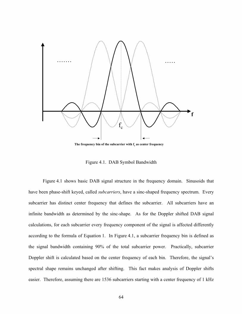
64

fc

The frequency bin of the subcarrier with fc as center frequency

. . . . . . . . . . . .

f

Figure 4.1. DAB Symbol Bandwidth

Figure 4.1 shows basic DAB signal structure in the frequency domain. Sinusoids that

have been phase-shift keyed, called subcarriers, have a sinc-shaped frequency spectrum. Every

subcarrier has distinct center frequency that defines the subcarrier. All subcarriers have an

infinite bandwidth as determined by the sinc-shape. As for the Doppler shifted DAB signal

calculations, for each subcarrier every frequency component of the signal is affected differently

according to the formula of Equation 1. In Figure 4.1, a subcarrier frequency bin is defined as

the signal bandwidth containing 90% of the total subcarrier power. Practically, subcarrier

Doppler shift is calculated based on the center frequency of each bin. Therefore, the signal’s

spectral shape remains unchanged after shifting. This fact makes analysis of Doppler shifts

easier. Therefore, assuming there are 1536 subcarriers starting with a center frequency of 1 kHz

65

at baseband, Doppler frequency may be calculated based on one single frequency located at the

center of the total DAB signal bandwidth. This approach has an inherent advantage in ambiguity

function calculation of the DAB waveform. Specifically, this approach enables us to use fast

DAB symbol creation algorithms based on IFFT and Doppler shifted signals are easily created

(Chapter 3).

The issue that one has to pay attention is the introduction of an error with the assumption

of constant Doppler frequency for all of the subcarriers. The next section deals with visualizing

the error caused by implementing the fast DAB waveform generation techniques explained

above, techniques which have been readily adopted by other researchers with minimal

justification [18].

To see the extent of the problem, two ambiguity surface generation techniques are

considered. For method one, a constant Doppler frequency shift resulting from a moving target is

assumed induced on each subcarrier, i.e., the amount of Doppler shift induced on each subcarrier

is independent of the actual subcarrier frequency. For method two, the ambiguity surface plot

represents the correct Doppler shifted signal in the simulation, i.e., in creating the Doppler

shifted signal the induced Doppler resulting from a moving target is calculated independently for

each subcarrier, the subcarriers are then added to form the composite Doppler shifted signal.

In analyzing three-dimensional ambiguity surface plots from both techniques, it is

impossible to visually discern any difference between the approaches. So, to do a comparison of

results from both approaches, the response along a principal axis of the surface is analyzed.

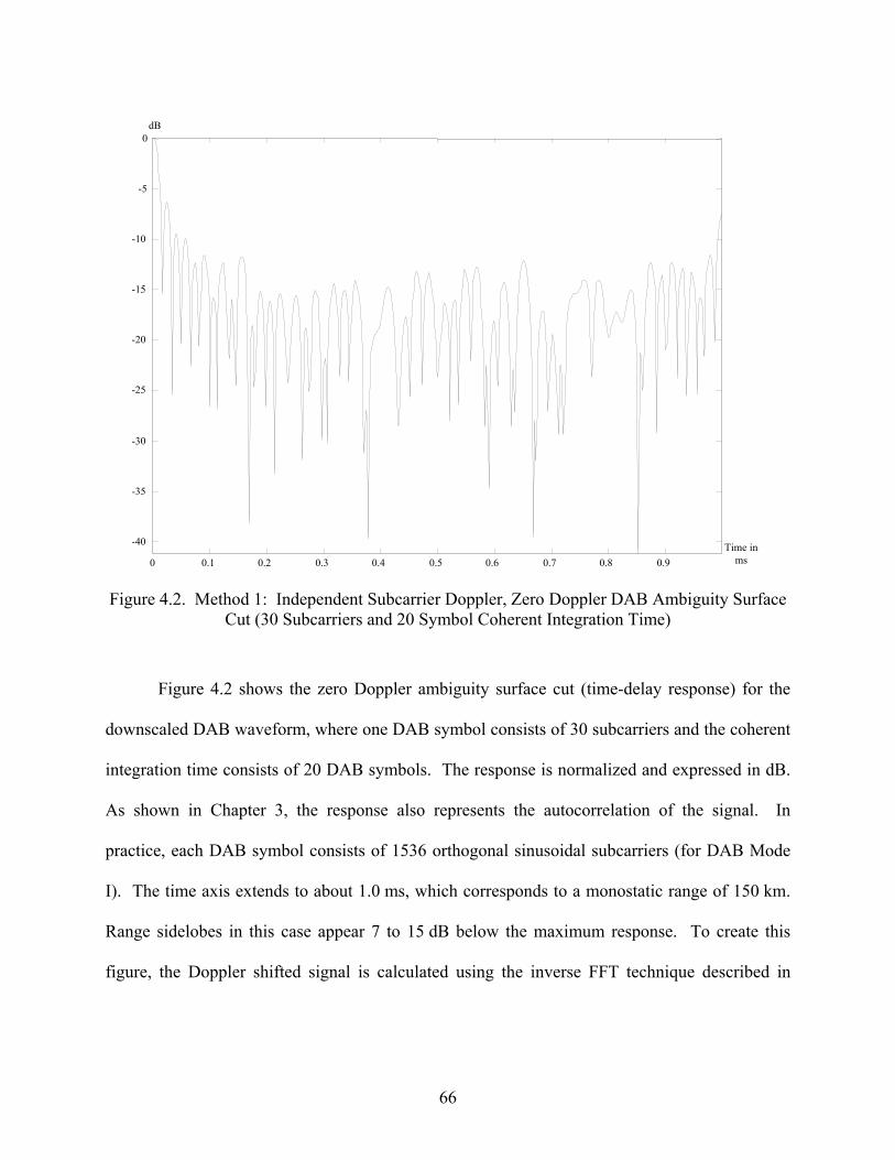
66

i i

0 0.1 0.2 0.3 0.4 0.5 0.6 0.7 0.8 0.9

-40

-35

-30

-25

-20

-15

-10

-5

0

Time inms

dB

Figure 4.2. Method 1: Independent Subcarrier Doppler, Zero Doppler DAB Ambiguity Surface

Cut (30 Subcarriers and 20 Symbol Coherent Integration Time)

Figure 4.2 shows the zero Doppler ambiguity surface cut (time-delay response) for the

downscaled DAB waveform, where one DAB symbol consists of 30 subcarriers and the coherent

integration time consists of 20 DAB symbols. The response is normalized and expressed in dB.

As shown in Chapter 3, the response also represents the autocorrelation of the signal. In

practice, each DAB symbol consists of 1536 orthogonal sinusoidal subcarriers (for DAB Mode

I). The time axis extends to about 1.0 ms, which corresponds to a monostatic range of 150 km.

Range sidelobes in this case appear 7 to 15 dB below the maximum response. To create this

figure, the Doppler shifted signal is calculated using the inverse FFT technique described in

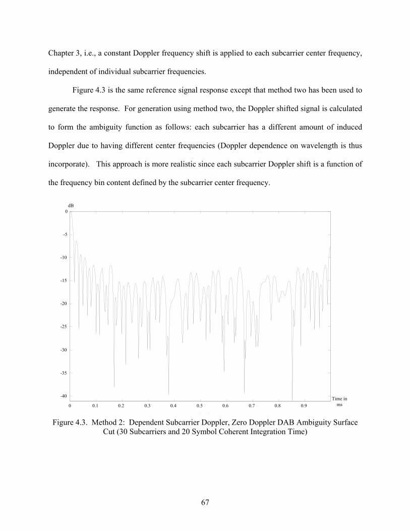
67

Chapter 3, i.e., a constant Doppler frequency shift is applied to each subcarrier center frequency,

independent of individual subcarrier frequencies.

Figure 4.3 is the same reference signal response except that method two has been used to

generate the response. For generation using method two, the Doppler shifted signal is calculated

to form the ambiguity function as follows: each subcarrier has a different amount of induced

Doppler due to having different center frequencies (Doppler dependence on wavelength is thus

incorporate). This approach is more realistic since each subcarrier Doppler shift is a function of

the frequency bin content defined by the subcarrier center frequency.

i i

0 0.1 0.2 0.3 0.4 0.5 0.6 0.7 0.8 0.9

-40

-35

-30

-25

-20

-15

-10

-5

0

Time inms

dB

Figure 4.3. Method 2: Dependent Subcarrier Doppler, Zero Doppler DAB Ambiguity Surface

Cut (30 Subcarriers and 20 Symbol Coherent Integration Time)

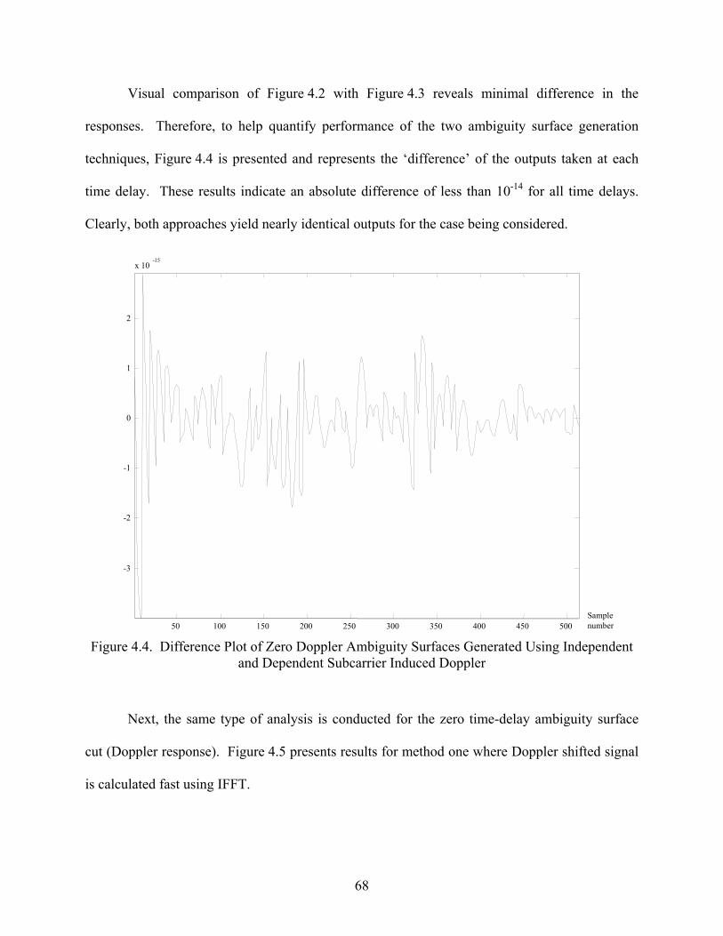
68

Visual comparison of Figure 4.2 with Figure 4.3 reveals minimal difference in the

responses. Therefore, to help quantify performance of the two ambiguity surface generation

techniques, Figure 4.4 is presented and represents the ‘difference’ of the outputs taken at each

time delay. These results indicate an absolute difference of less than 10-14 for all time delays.

Clearly, both approaches yield nearly identical outputs for the case being considered.

50 100 150 200 250 300 350 400 450 500

-3

-2

-1

0

1

2

x 10-15

Samplenumber

Figure 4.4. Difference Plot of Zero Doppler Ambiguity Surfaces Generated Using Independent and Dependent Subcarrier Induced Doppler

Next, the same type of analysis is conducted for the zero time-delay ambiguity surface

cut (Doppler response). Figure 4.5 presents results for method one where Doppler shifted signal

is calculated fast using IFFT.

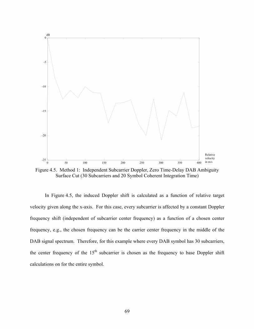
69

0 50 100 150 200 250 300 350 400-25

-20

-15

-10

-5

0

Relativevelocityin m/s

dB

Figure 4.5. Method 1: Independent Subcarrier Doppler, Zero Time-Delay DAB Ambiguity

Surface Cut (30 Subcarriers and 20 Symbol Coherent Integration Time)

In Figure 4.5, the induced Doppler shift is calculated as a function of relative target

velocity given along the x-axis. For this case, every subcarrier is affected by a constant Doppler

frequency shift (independent of subcarrier center frequency) as a function of a chosen center

frequency, e.g., the chosen frequency can be the carrier center frequency in the middle of the

DAB signal spectrum. Therefore, for this example where every DAB symbol has 30 subcarriers,

the center frequency of the 15th subcarrier is chosen as the frequency to base Doppler shift

calculations on for the entire symbol.

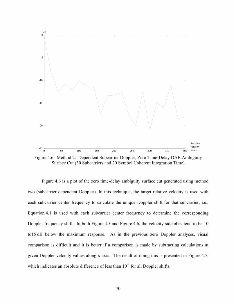
70

0 50 100 150 200 250 300 350 400-25

-20

-15

-10

-5

0

Relativevelocityin m/s

dB

Figure 4.6. Method 2: Dependent Subcarrier Doppler, Zero Time-Delay DAB Ambiguity

Surface Cut (30 Subcarriers and 20 Symbol Coherent Integration Time)

Figure 4.6 is a plot of the zero time-delay ambiguity surface cut generated using method

two (subcarrier dependent Doppler). In this technique, the target relative velocity is used with

each subcarrier center frequency to calculate the unique Doppler shift for that subcarrier, i.e.,

Equation 4.1 is used with each subcarrier center frequency to determine the corresponding

Doppler frequency shift. In both Figure 4.5 and Figure 4.6, the velocity sidelobes tend to be 10

to15 dB below the maximum response. As in the previous zero Doppler analyses, visual

comparison is difficult and it is better if a comparison is made by subtracting calculations at

given Doppler velocity values along x-axis. The result of doing this is presented in Figure 4.7,

which indicates an absolute difference of less than 10-4 for all Doppler shifts.

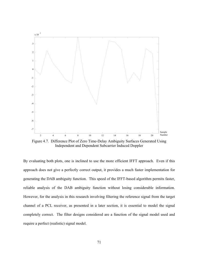
71

2 4 6 8 10 12 14 16 18 20

-7

-6

-5

-4

-3

-2

-1

0

1

2

3

x 10-5

SampleNumber

Figure 4.7. Difference Plot of Zero Time-Delay Ambiguity Surfaces Generated Using Independent and Dependent Subcarrier Induced Doppler

By evaluating both plots, one is inclined to use the more efficient IFFT approach. Even if this

approach does not give a perfectly correct output, it provides a much faster implementation for

generating the DAB ambiguity function. This speed of the IFFT-based algorithm permits faster,

reliable analysis of the DAB ambiguity function without losing considerable information.

However, for the analysis in this research involving filtering the reference signal from the target

channel of a PCL receiver, as presented in a later section, it is essential to model the signal

completely correct. The filter designs considered are a function of the signal model used and

require a perfect (realistic) signal model.

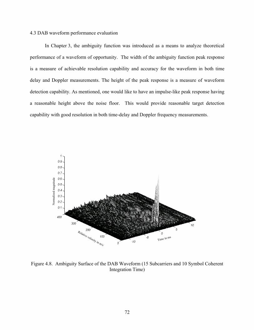
72

4.3 DAB waveform performance evaluation

In Chapter 3, the ambiguity function was introduced as a means to analyze theoretical

performance of a waveform of opportunity. The width of the ambiguity function peak response

is a measure of achievable resolution capability and accuracy for the waveform in both time

delay and Doppler measurements. The height of the peak response is a measure of waveform

detection capability. As mentioned, one would like to have an impulse-like peak response having

a reasonable height above the noise floor. This would provide reasonable target detection

capability with good resolution in both time-delay and Doppler frequency measurements.

Relative velocity in m/sTime in ms

Nor

mal

ize d

mag

nitu

de

Figure 4.8. Ambiguity Surface of the DAB Waveform (15 Subcarriers and 10 Symbol Coherent

Integration Time)

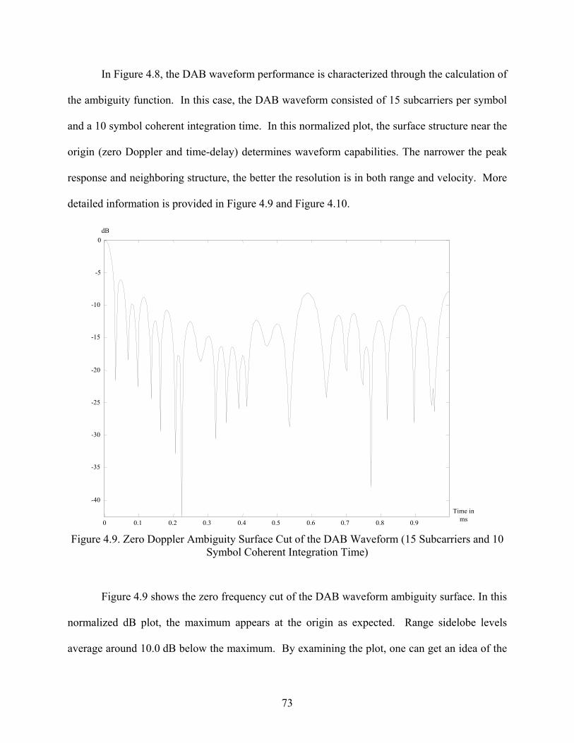
73

In Figure 4.8, the DAB waveform performance is characterized through the calculation of

the ambiguity function. In this case, the DAB waveform consisted of 15 subcarriers per symbol

and a 10 symbol coherent integration time. In this normalized plot, the surface structure near the

origin (zero Doppler and time-delay) determines waveform capabilities. The narrower the peak

response and neighboring structure, the better the resolution is in both range and velocity. More

detailed information is provided in Figure 4.9 and Figure 4.10.

0 0.1 0.2 0.3 0.4 0.5 0.6 0.7 0.8 0.9

-40

-35

-30

-25

-20

-15

-10

-5

0dB

Time inms

Figure 4.9. Zero Doppler Ambiguity Surface Cut of the DAB Waveform (15 Subcarriers and 10 Symbol Coherent Integration Time)

Figure 4.9 shows the zero frequency cut of the DAB waveform ambiguity surface. In this

normalized dB plot, the maximum appears at the origin as expected. Range sidelobe levels

average around 10.0 dB below the maximum. By examining the plot, one can get an idea of the

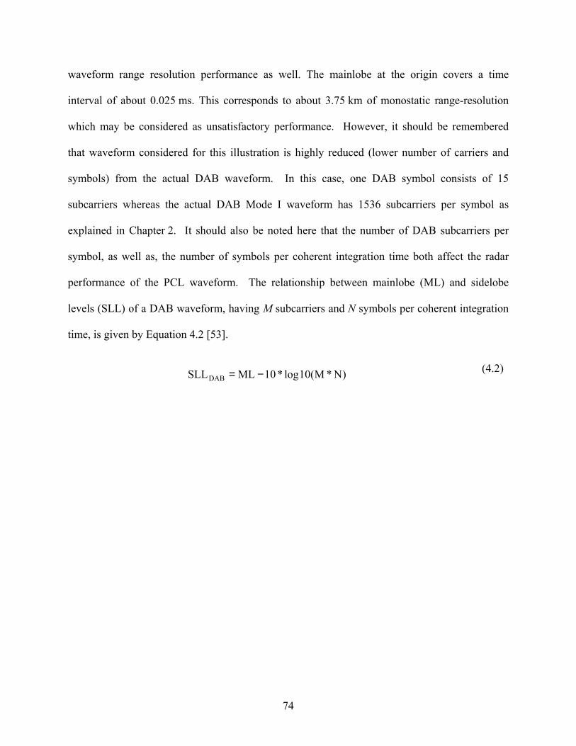
74

waveform range resolution performance as well. The mainlobe at the origin covers a time

interval of about 0.025 ms. This corresponds to about 3.75 km of monostatic range-resolution

which may be considered as unsatisfactory performance. However, it should be remembered

that waveform considered for this illustration is highly reduced (lower number of carriers and

symbols) from the actual DAB waveform. In this case, one DAB symbol consists of 15

subcarriers whereas the actual DAB Mode I waveform has 1536 subcarriers per symbol as

explained in Chapter 2. It should also be noted here that the number of DAB subcarriers per

symbol, as well as, the number of symbols per coherent integration time both affect the radar

performance of the PCL waveform. The relationship between mainlobe (ML) and sidelobe

levels (SLL) of a DAB waveform, having M subcarriers and N symbols per coherent integration

time, is given by Equation 4.2 [53].

)N*M(10log*10MLSLLDAB −= (4.2)

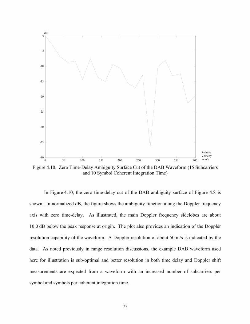
75

0 50 100 150 200 250 300 350 400-40

-35

-30

-25

-20

-15

-10

-5

0dB

RelativeVelocityin m/s

Figure 4.10. Zero Time-Delay Ambiguity Surface Cut of the DAB Waveform (15 Subcarriers and 10 Symbol Coherent Integration Time)

In Figure 4.10, the zero time-delay cut of the DAB ambiguity surface of Figure 4.8 is

shown. In normalized dB, the figure shows the ambiguity function along the Doppler frequency

axis with zero time-delay. As illustrated, the main Doppler frequency sidelobes are about

10.0 dB below the peak response at origin. The plot also provides an indication of the Doppler

resolution capability of the waveform. A Doppler resolution of about 50 m/s is indicated by the

data. As noted previously in range resolution discussions, the example DAB waveform used

here for illustration is sub-optimal and better resolution in both time delay and Doppler shift

measurements are expected from a waveform with an increased number of subcarriers per

symbol and symbols per coherent integration time.

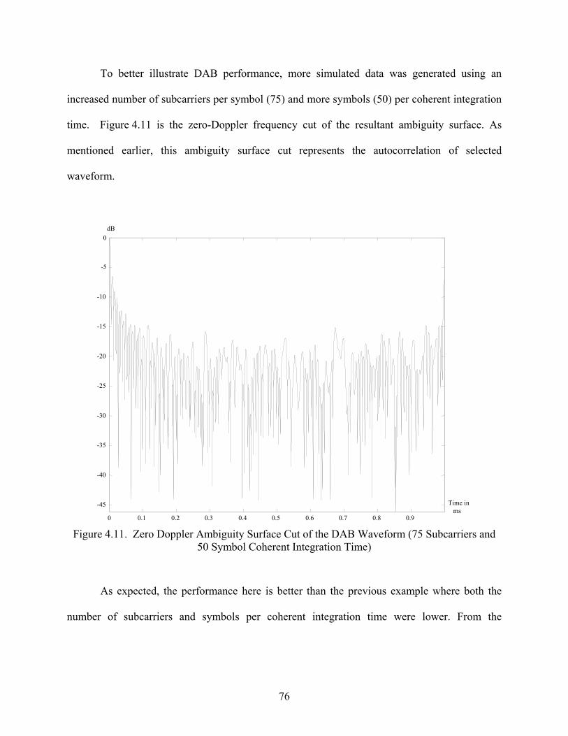
76

To better illustrate DAB performance, more simulated data was generated using an

increased number of subcarriers per symbol (75) and more symbols (50) per coherent integration

time. Figure 4.11 is the zero-Doppler frequency cut of the resultant ambiguity surface. As

mentioned earlier, this ambiguity surface cut represents the autocorrelation of selected

waveform.

0 0.1 0.2 0.3 0.4 0.5 0.6 0.7 0.8 0.9

-45

-40

-35

-30

-25

-20

-15

-10

-5

0

Time inms

dB

Figure 4.11. Zero Doppler Ambiguity Surface Cut of the DAB Waveform (75 Subcarriers and

50 Symbol Coherent Integration Time)

As expected, the performance here is better than the previous example where both the

number of subcarriers and symbols per coherent integration time were lower. From the

77

Figure 4.11, the sidelobe levels are approximately 15 to 20 dB below the peak response at the

origin – approximately a 5.0 to 10.0 dB improvement over the previous case.

0 50 100 150 200 250 300 350 400-25

-20

-15

-10

-5

0dB

RelativeVelocityin m/s

Figure 4.12. Zero Time-Delay Cut of DAB Waveform Ambiguity Surface

Figure 4.12 is the zero time-delay cut of the DAB ambiguity surface for the new DAB

waveform. This axis could be replaced with Doppler shift frequency axis for the case where the

Doppler shifted signal is calculated as having a constant Doppler frequency on every subcarrier.

The velocity resolution is now approximately 25 m/s and the sidelobe levels are around 15 to

20 dB lower than the peak at the maximum – approximately a 5.0 to 10.0 dB improvement over

the previous case.

78

The zero-cut ambiguity surface performance results presented here for the DAB

waveform closely matches calculations available from the literature [18]. In fact, there are only

a few open literature sources for comparison of results.

The DAB waveform performance, as supported by previous data plots and calculations

above, is encouraging. It is anticipated that the accuracy and resolution in both time and

frequency measurements will be quite good for the real DAB waveform, given it consists of

1536 subcarriers per symbol. In practice, there will be certain challenges to deal with in order to

fully exploit benefits of the DAB waveform.

4.4 DAB detection surfaces

A receiver dedicated to exploiting PCL DAB signals may use a matched filter for signal

processing and target detection. In this particular signal-processing scheme, at least two receiver

channels are necessary. One channel is dedicated to receiving the reference waveform, defined

as the direct break-through of a transmitted signal from the closest line-of-sight (LOS)

transmitter to the PCL receiver. The second receiver channel is target channel, i.e., the antenna

of this receiver channel is specifically directed towards a surveillance region to receive target

returns (echoes) of the reference waveform returning from targets. The target returns are simply

time-delayed, Doppler-shifted versions of the reference waveform. If the reference waveform

can be written as a closed-form mathematical expression, then a target response can be easily

created by simply incorporating desired time delay and frequency shift to resemble a target

return.

The above-described signal-processing scheme is similar to the process implemented for

calculating the ambiguity function, as explained earlier. The ambiguity surfaces calculated

earlier represented the correlation of a reference DAB waveform with a time delayed and

79

Doppler shifted versions of itself. Therefore, the peak response appeared at the origin

corresponding to no time delay and no Doppler shift. In this new implementation, the reference

waveform is both time delayed and frequency shifted before being correlated with the target

channel output.

In general, the target channel output consists of the reference signal having unknown time

delay and Doppler frequency shift, as induced by the target range and velocity parameters. In

this case, the peak in the ambiguity surface appears at a location (time delay and Doppler)

corresponding to the reference waveform having the same phase and frequency characteristics as

the target signal. Therefore, by tracking the time-frequency shifts induced on reference

waveform, one is able to determine the corresponding target parameters affecting the signal

received in the receiver target channel.

80

Time in ms

Relative velocity in m/s

Det

ecti o

n s u

r face

mag

nit u

de

Figure 4.13. Target Channel Detection Surface – Target Present (30 Subcarriers and 20 Symbol

coherent Integration Time)

Figure 4.13 is a target channel detection surface generated to illustrate the approach

explained above. In this case, the DAB waveform consists of 30 subcarriers per symbol and 20

symbols per coherent integration time. The simulated target channel signal in this example only

consists of a target response. The target is assumed to have a relative velocity of 200 m/s in a

monostatic sense, i.e., the target’s radial velocity is assumed to be 200 m/s with respect to

transmitter/receiver site. As indicated, the surface in Figure 4.13 is technically not an ambiguity

surface but rather a detection surface, i.e., a surface generated using techniques similar to

ambiguity function calculations. The detection surface provides theoretical insight into how well

a particular waveform may perform in the detection and estimation of targets. In this case, the

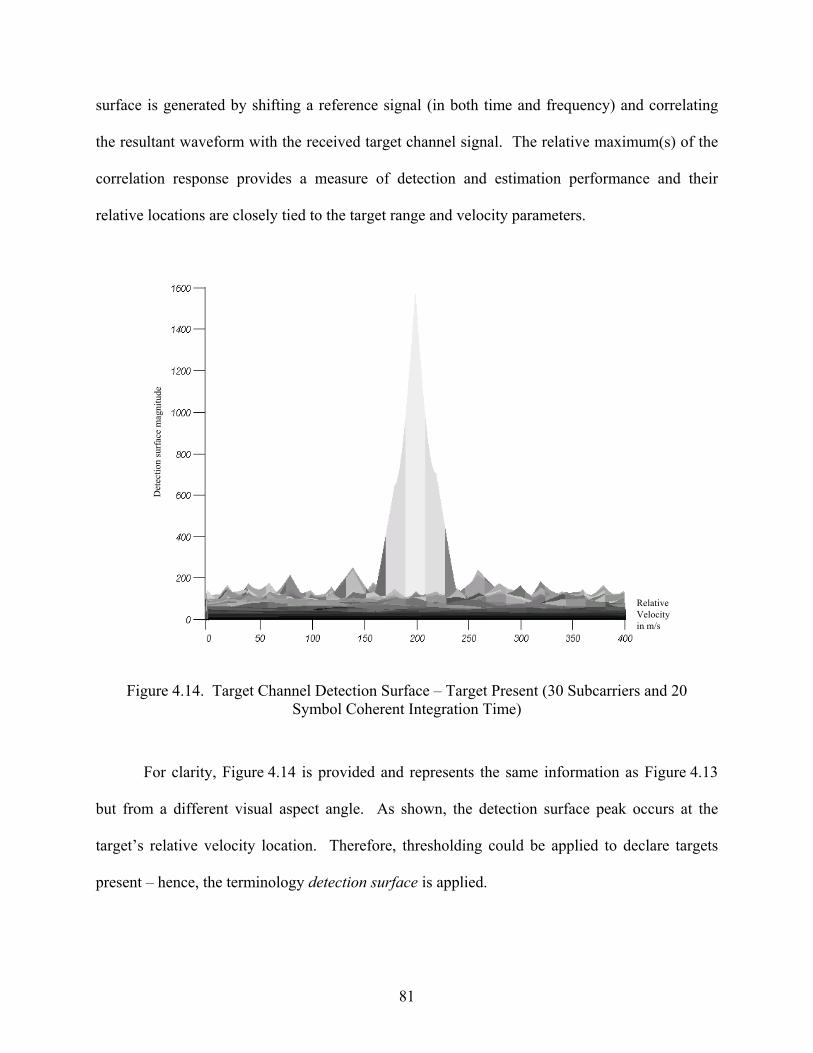
81

surface is generated by shifting a reference signal (in both time and frequency) and correlating

the resultant waveform with the received target channel signal. The relative maximum(s) of the

correlation response provides a measure of detection and estimation performance and their

relative locations are closely tied to the target range and velocity parameters.

Det

ect io

n su

rface

ma g

n itu

d e

RelativeVelocityin m/s

Figure 4.14. Target Channel Detection Surface – Target Present (30 Subcarriers and 20

Symbol Coherent Integration Time)

For clarity, Figure 4.14 is provided and represents the same information as Figure 4.13

but from a different visual aspect angle. As shown, the detection surface peak occurs at the

target’s relative velocity location. Therefore, thresholding could be applied to declare targets

present – hence, the terminology detection surface is applied.

82

In practice, the received target channel signal does not only include target returns but also

noise. The model chosen to reflect the channel noise contribution is Gaussian, although, the

particular choice of this model does not influence research results.

Another signal component present in the received target channel is the reference signal

itself. Therefore, even if it is not intended to have the reference signal at the target channel

output, practically it is not possible to isolate the target channel from the reference. The effects

of this component, which could be defined as the leakage of the reference signal into the target

channel, highly degrade the performance of the system. Theoretical analysis of this degradation

is implemented in Chapter 3.

The DAB transmitter architecture is built in accordance with the needs of Single Frequency

Networks (SFN). As explained earlier, in the commercial DAB architecture the transmitters are

a certain distance from each other as dictated by the required guard interval of DAB waveform

(see Chapter 2). For a PCL receiver, this means that in the received signal, along with the

reference signal from the main transmitter closest to the receiver, there are time-delayed replicas

of the reference signal due to other transmitters in the vicinity. These replica signals are lower in

power since they are from transmitters located further away from the receiver. For this research,

these replica components are treated as nothing more than a multipath reflection of the reference

signal as received from each distant transmitter in the SFN structure.

As a result of the discussion above, four components of the PCL receiver target channel can

be distinguished:

1. The return of the transmitted DAB signal from the target, (this component can be

thought as Doppler and time (phase) shifted version of the reference signal),

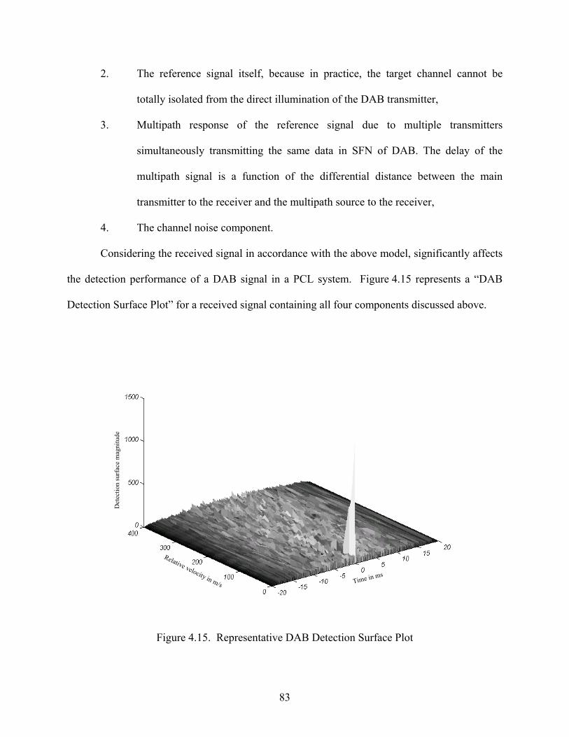
83

2. The reference signal itself, because in practice, the target channel cannot be

totally isolated from the direct illumination of the DAB transmitter,

3. Multipath response of the reference signal due to multiple transmitters

simultaneously transmitting the same data in SFN of DAB. The delay of the

multipath signal is a function of the differential distance between the main

transmitter to the receiver and the multipath source to the receiver,

4. The channel noise component.

Considering the received signal in accordance with the above model, significantly affects

the detection performance of a DAB signal in a PCL system. Figure 4.15 represents a “DAB

Detection Surface Plot” for a received signal containing all four components discussed above.

Time in ms

Relative velocity in m/s

Det

ectio

n su

rface

mag

nitu

de

Figure 4.15. Representative DAB Detection Surface Plot

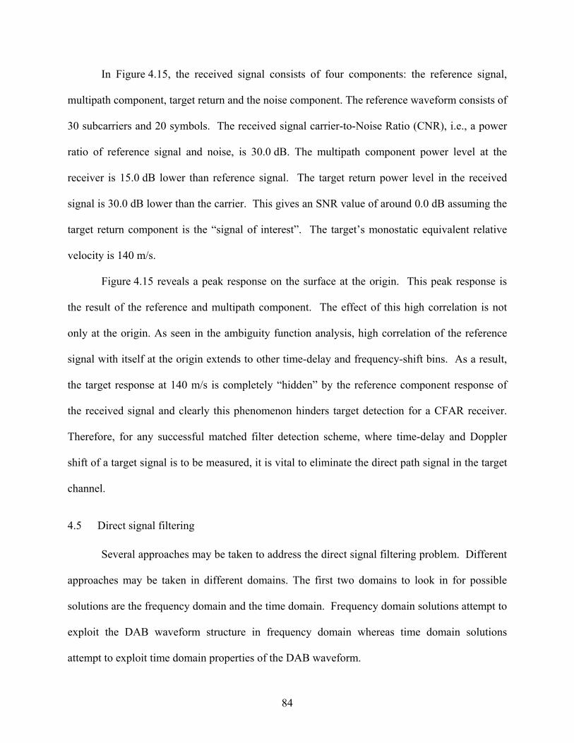
84

In Figure 4.15, the received signal consists of four components: the reference signal,

multipath component, target return and the noise component. The reference waveform consists of

30 subcarriers and 20 symbols. The received signal carrier-to-Noise Ratio (CNR), i.e., a power

ratio of reference signal and noise, is 30.0 dB. The multipath component power level at the

receiver is 15.0 dB lower than reference signal. The target return power level in the received

signal is 30.0 dB lower than the carrier. This gives an SNR value of around 0.0 dB assuming the

target return component is the “signal of interest”. The target’s monostatic equivalent relative

velocity is 140 m/s.

Figure 4.15 reveals a peak response on the surface at the origin. This peak response is

the result of the reference and multipath component. The effect of this high correlation is not

only at the origin. As seen in the ambiguity function analysis, high correlation of the reference

signal with itself at the origin extends to other time-delay and frequency-shift bins. As a result,

the target response at 140 m/s is completely “hidden” by the reference component response of

the received signal and clearly this phenomenon hinders target detection for a CFAR receiver.

Therefore, for any successful matched filter detection scheme, where time-delay and Doppler

shift of a target signal is to be measured, it is vital to eliminate the direct path signal in the target

channel.

4.5 Direct signal filtering

Several approaches may be taken to address the direct signal filtering problem. Different

approaches may be taken in different domains. The first two domains to look in for possible

solutions are the frequency domain and the time domain. Frequency domain solutions attempt to

exploit the DAB waveform structure in frequency domain whereas time domain solutions

attempt to exploit time domain properties of the DAB waveform.

85

An initial look into frequency domain techniques did not seem promising. First, the DAB

signal has a relatively large bandwidth of 1.5 MHz. Any filter designed in frequency domain

would need to differentiate between the reference signal and the target component of the

received signal in the frequency domain. The target return in frequency domain basically

appears as a shifted version of reference signal, with the amount of Doppler frequency shift is

associated with target relative velocity.

DAB signal frequency domainDoppler shifted DAB signal

f Figure 4.16. Frequency Domain Response of DAB Direct Signal and Doppler Shifted

Target Return

One can infer from Figure 4.16 that for reasonable Doppler frequencies, i.e., those

generated from velocities of typical airborne platforms, it is not possible to use narrowband-

86

filtering techniques of traditional radar signal processing to eliminate the reference signal

response. Traditional solutions including frequency domain IIR and FIR filtering seem

impractical for eliminating the reference signal while passing the target return unaltered.

If working in the time domain, more interesting approaches can be considered. One idea

involves using intelligent signal processing schemes from the world of Artificial Neural

Networks (ANN) [24].

Another unique solution was implemented as part of this research and comes from the

basic idea of a matrix projection operation. Detailed background material about this projection

operation is presented in Chapter 3. Basically, the idea is to “project” the received signal into an

alternate space that is orthogonal to the direct path signal. Ideally, this projection eliminates the

direct path component from the projected signal while having minimal affect on the desired

target return. Target detection is then implemented using the resultant signal from the projection

operation of the received signal. There are several questions that have to be answered in this

signal-processing algorithm:

1. Does the projection operator completely eliminate the direct path signal consisting of

a reference component together with multipath component?

2. Does the projection preserve the desired target return component?

3. How can the projection operation be implemented for the DAB waveform?

What one wants is a design that completely eliminates the reference and multipath

component, where the multipath component is simply a time-delayed version of the reference

component. It is also desirable for the target return component of the received waveform to pass

87

through the filtering unchanged. Of course, these are ideal considerations and practically any

realizable filter implementation will not be able to completely eliminate the direct-path signal.

As with all filter designs, the projection operation technique will probably attenuate target

returns as well.

Considering the discussion on projection operation effects, a new set of goals is

introduced. Namely, one wants the direct-path signal to be sufficiently attenuated such that its

response on the detection surface does not hinder target detection, i.e., it does not have a

response that “hides” the desired response at time delay and Doppler shift values consistent with

the target’s parameters. This effect was illustrated in Figure 4.15 and subsequently discussed.

Another important criterion for evaluating practical filter performance is the evaluation of

Signal-to-Noise Ratios (SNR) before and after filtering. For this work, the “signal of interest” is

the target return component of the received signal. Although there will be signal attenuation

during filtering, the resultant SNR values after filtering should be at reasonable levels to enable

target detection and parametric estimation. This brings another consideration into play, namely,

what is the projection operation effect on the noise component of the received signal?

Details of the proposed time domain projection filter are included in Chapter 3, where

information about the exploitation of DAB signal structure to form the projection operation is

explained. Simulation results for the proposed projection filter approach are presented next.

4.6 Simulations

The simulation results presented in this section are for two different scenarios. The first

scenario is an ideal scenario where the phase reference symbol transmitted in every frame is

demodulated under ideal conditions, i.e., the phase reference for every subcarrier, as used by the

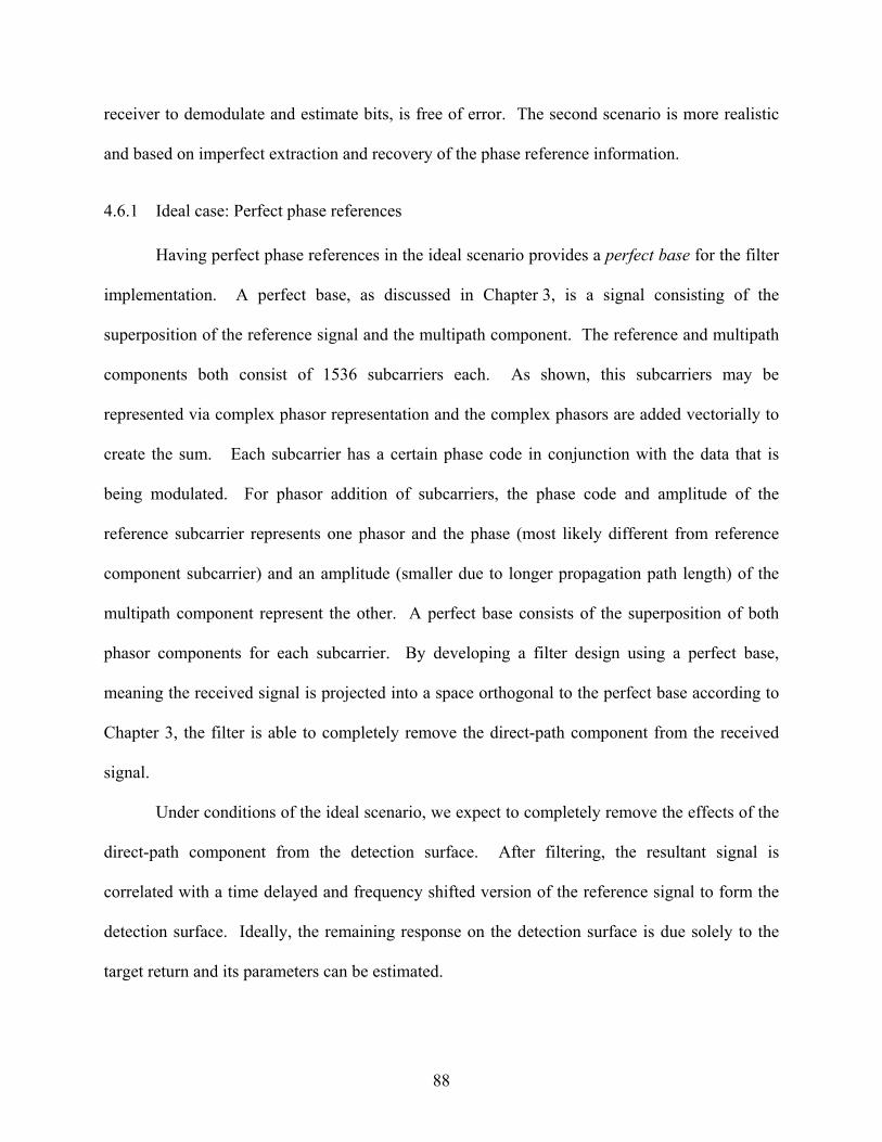
88

receiver to demodulate and estimate bits, is free of error. The second scenario is more realistic

and based on imperfect extraction and recovery of the phase reference information.

4.6.1 Ideal case: Perfect phase references

Having perfect phase references in the ideal scenario provides a perfect base for the filter

implementation. A perfect base, as discussed in Chapter 3, is a signal consisting of the

superposition of the reference signal and the multipath component. The reference and multipath

components both consist of 1536 subcarriers each. As shown, this subcarriers may be

represented via complex phasor representation and the complex phasors are added vectorially to

create the sum. Each subcarrier has a certain phase code in conjunction with the data that is

being modulated. For phasor addition of subcarriers, the phase code and amplitude of the

reference subcarrier represents one phasor and the phase (most likely different from reference

component subcarrier) and an amplitude (smaller due to longer propagation path length) of the

multipath component represent the other. A perfect base consists of the superposition of both

phasor components for each subcarrier. By developing a filter design using a perfect base,

meaning the received signal is projected into a space orthogonal to the perfect base according to

Chapter 3, the filter is able to completely remove the direct-path component from the received

signal.

Under conditions of the ideal scenario, we expect to completely remove the effects of the

direct-path component from the detection surface. After filtering, the resultant signal is

correlated with a time delayed and frequency shifted version of the reference signal to form the

detection surface. Ideally, the remaining response on the detection surface is due solely to the

target return and its parameters can be estimated.

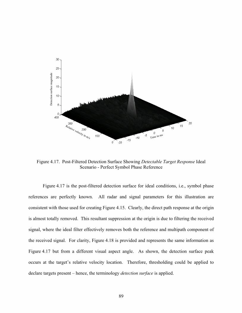
89

Time in ms

Relative velocity in m/s

Det

ectio

n su

rface

mag

nitu

de

Figure 4.17. Post-Filtered Detection Surface Showing Detectable Target Response Ideal

Scenario - Perfect Symbol Phase Reference

Figure 4.17 is the post-filtered detection surface for ideal conditions, i.e., symbol phase

references are perfectly known. All radar and signal parameters for this illustration are

consistent with those used for creating Figure 4.15. Clearly, the direct path response at the origin

is almost totally removed. This resultant suppression at the origin is due to filtering the received

signal, where the ideal filter effectively removes both the reference and multipath component of

the received signal. For clarity, Figure 4.18 is provided and represents the same information as

Figure 4.17 but from a different visual aspect angle. As shown, the detection surface peak

occurs at the target’s relative velocity location. Therefore, thresholding could be applied to

declare targets present – hence, the terminology detection surface is applied.

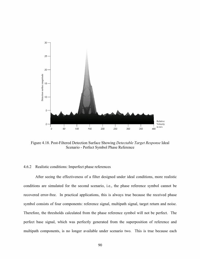
90

Det

ectio

n su

rface

mag

nitu

de

RelativeVelocityin m/s

Figure 4.18. Post-Filtered Detection Surface Showing Detectable Target Response Ideal

Scenario - Perfect Symbol Phase Reference

4.6.2 Realistic conditions: Imperfect phase references

After seeing the effectiveness of a filter designed under ideal conditions, more realistic

conditions are simulated for the second scenario, i.e., the phase reference symbol cannot be

recovered error-free. In practical applications, this is always true because the received phase

symbol consists of four components: reference signal, multipath signal, target return and noise.

Therefore, the thresholds calculated from the phase reference symbol will not be perfect. The

perfect base signal, which was perfectly generated from the superposition of reference and

multipath components, is no longer available under scenario two. This is true because each

91

received subcarrier is now the superposition of a reference signal, multipath components, a target

return (assuming a target is present) and a channel noise component. This is shown in Chapter 2.

The filter design implemented using this new imperfect base signal will not be able to

totally remove the direct-path component. The transformation space defined by the orthogonal

projection of the received signal is now orthogonal to the imperfect base signal comprised of

components other than the direct-path. This effectively causes a leakage of the reference and

multipath components into the projected signal, as well as, more significant attenuation of the

desired target return.

-10

0 10

Time in ms

300 200

100

Relative velocity in m/s

Det

ecti o

n s u

rface

mag

n itu

d e

Figure 4.19. Pre-Filtered Detection Surface Showing Undetectable Target Response

Non-Ideal Scenario - Imperfect Symbol Phase Reference

92

Figure 4.19 is the pre-filtered detection surface for non-ideal conditions, i.e., symbol

phase references are not perfectly known. As before, the received signal has a direct signal

reference component that is 30.0 dB above both the target return and the noise component, and it

is 10.0 dB higher than the multipath component. Because of direct path dominance in the

received signal, the only discernable peak appears near the origin, just like an ambiguity surface

plot. For clarity, Figure 4.20 is provided and represents the same information as Figure 4.19 but

from a different visual aspect angle. As shown, the unfiltered response near the origin

completely dominates and the target response is undetectable.

20 60 100 140 180 220 260 300 340 380

RelativeVelocityin m/s

Det

ectio

n su

r fac

e m

agni

t ude

Figure 4.20. Pre-Filtered Detection Surface Showing Undetectable Target Response

Non-Ideal Scenario - Imperfect Symbol Phase Reference (side view)

93

Figure 4.21, is the plot of the post-filtered detection surface. A better plot showing the

effect of filtering is Figure 4.22. Care must be taken in analyzing this example, the direct path

response on the detection surface is not completely removed.

-10

0 10

Time in ms

300 200

100

Relative velocity in m/s

Det

ecti o

n s u

rface

mag

n itu

d e

Figure 4.21. Post-Filtered Detection Surface Showing Detectable Target Response Non-

Ideal Scenario - Imperfect Symbol Phase Reference

One encouraging fact that shows the efficiency of this filtering approach is that

the target response is now visible. The target detection performance increase is a result

of filtering the received signal direct-path component. Thus, a qualitative performance

analysis is necessary to see the filter design effectiveness.

For this, an example situation is considered where the received signal consists of

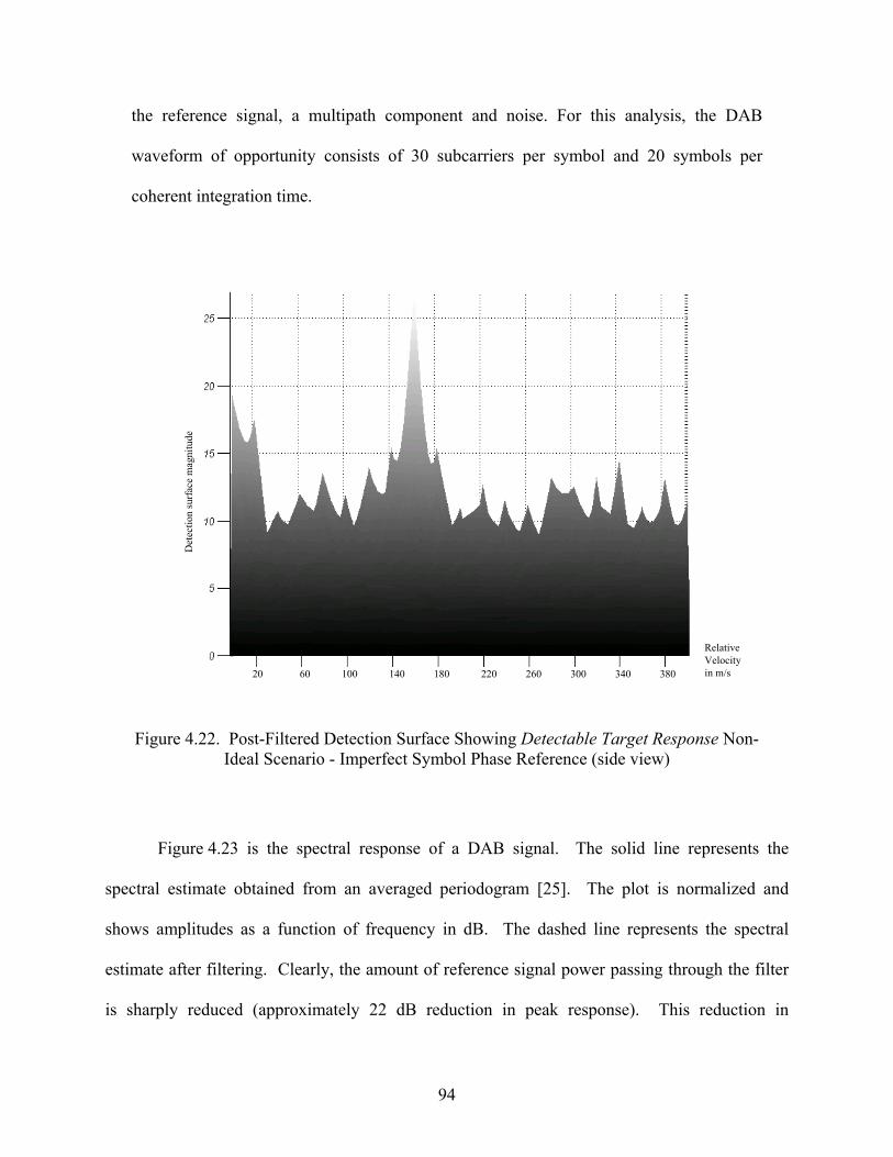
94

the reference signal, a multipath component and noise. For this analysis, the DAB

waveform of opportunity consists of 30 subcarriers per symbol and 20 symbols per

coherent integration time.

20 60 100 140 180 220 260 300 340 380

RelativeVelocityin m/s

Det

ectio

n su

rface

mag

nitu

de

Figure 4.22. Post-Filtered Detection Surface Showing Detectable Target Response Non-

Ideal Scenario - Imperfect Symbol Phase Reference (side view)

Figure 4.23 is the spectral response of a DAB signal. The solid line represents the

spectral estimate obtained from an averaged periodogram [25]. The plot is normalized and

shows amplitudes as a function of frequency in dB. The dashed line represents the spectral

estimate after filtering. Clearly, the amount of reference signal power passing through the filter

is sharply reduced (approximately 22 dB reduction in peak response). This reduction in

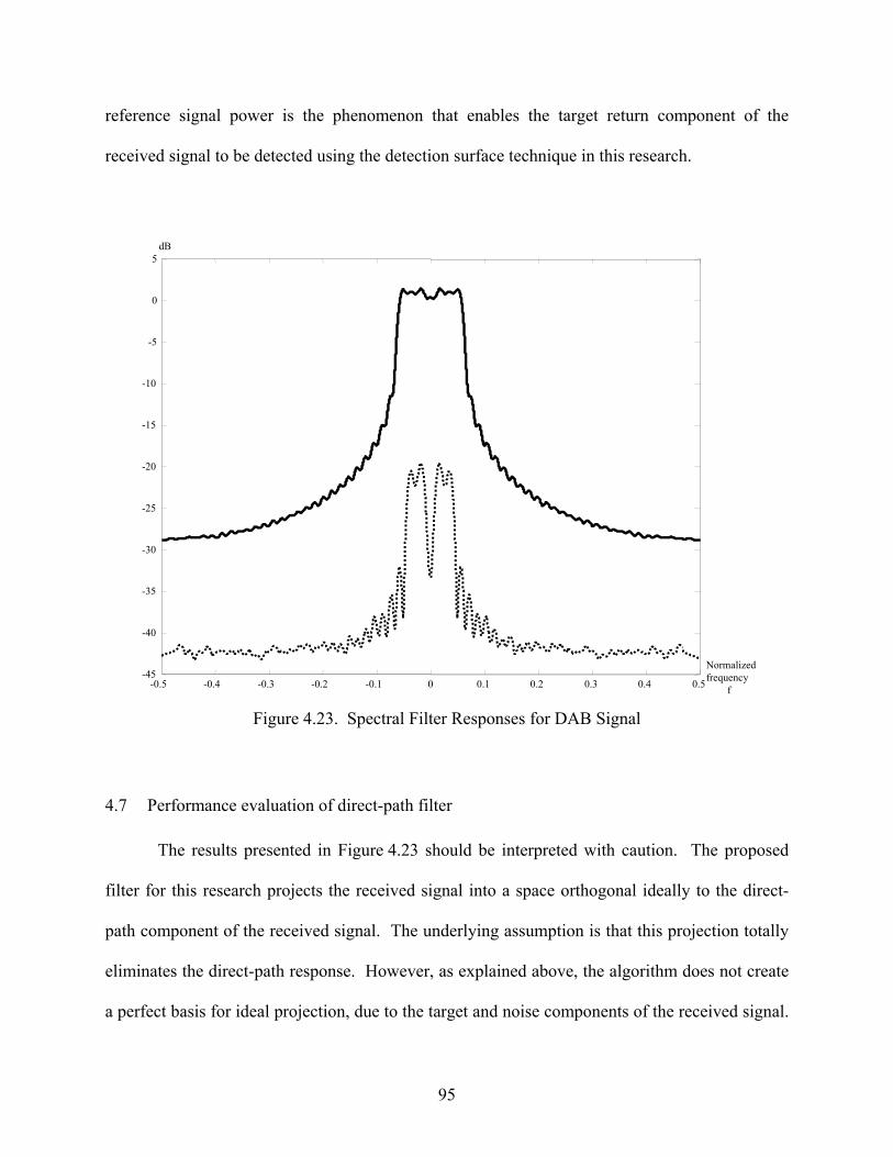
95

reference signal power is the phenomenon that enables the target return component of the

received signal to be detected using the detection surface technique in this research.

-0.5 -0.4 -0.3 -0.2 -0.1 0 0.1 0.2 0.3 0.4 0.5-45

-40

-35

-30

-25

-20

-15

-10

-5

0

5dB

Normalizedfrequency

f Figure 4.23. Spectral Filter Responses for DAB Signal

4.7 Performance evaluation of direct-path filter

The results presented in Figure 4.23 should be interpreted with caution. The proposed

filter for this research projects the received signal into a space orthogonal ideally to the direct-

path component of the received signal. The underlying assumption is that this projection totally

eliminates the direct-path response. However, as explained above, the algorithm does not create

a perfect basis for ideal projection, due to the target and noise components of the received signal.

96

Also, the target component itself is not perfectly orthogonal to the direct-path. Thus, the target

component will be attenuated by this projection operation, as well as, the noise component.

Therefore, a qualitative analysis of various attenuation levels for signal components is necessary

and follows.

In Figure 4.20, a pre-filtered detection surface is plotted for the received signal. The peak

response level occurs at the origin and is approximately 31.47 dB. When considering the

detection surface response at the origin after filtering, as in Figure 4.22, the level is about

12.55 dB. Therefore, a reduction of 18.92 dB can be associated with the direct path response of

the detection surface.

Similar analysis can be done for a target response on the detection surface. Before

filtering, the target response was 22.12 dB. After filtering, the detection surface is similar to

Figure 4.22 and the target response is approximately 14.31 dB. The target response is reduced

by approximately 7.81 dB.

Similarly, the noise floor is attenuated by the filtering process and causes a change in

SNR after filtering. As a measure of noise floor attenuation, every pre-filtered detection surface

component is added and compared to the sum of detection response components after filtering.

When done, the attenuation of the noise floor attenuation is around 11.0 dB. This simple analysis

technique provides an idea of potential noise floor reduction, although a rigorous proof of the

same is not provided.

The numbers calculated highlight the effectiveness of the filter. Although all received

signal components are attenuated, including the desired target return, the interfering direct path

component is attenuated much more significantly. Effectively, the higher direct path attenuation

results into an 11.11 dB accentuation of the target response, relative to the direct path response,

97

on the detection surface. Also, the detection surface noise floor is attenuated more than target

response.

4.8 Summary

In this chapter the proposed direct path filtering approach introduced in Chapter 3 was

simulated and its performance characterized. It was found to effectively eliminate (or

significantly reduce) the direct-path signal in the target channel of a PCL receiver containing

direct-path, target return and noise components.

The chapter started with the performance evaluation of DAB waveform as a PCL

waveform of opportunity. It has been found that with DAB has encouraging ambiguity function

properties. Time-delay and Doppler shift measurement accuracy and resolution can be dealt

independently and both can be improved simultaneously. Range and frequency sidelobe levels

are found to be a function of the number of subcarriers and the number of symbols per coherent

integration time. Equation 4.3 has been shown to be consistent with theoretical calculations

implemented for this research.

)N*M(10log*10MLSLLDAB −= (4.3)

In Equation 4.3, SLL is the DAB sidelobe level in dB, ML is the mainlobe level in dB, M

is the number of subcarriers per symbol and N the number of symbols per integration time.

A serious problem in a practical DAB PCL system implementation is identified, i.e., the

existence of a strong direct-path component in the PCL receiver target channel. A unique time

domain filtering technique has been proposed to eliminate this (Chapter 3) and its performance

evaluated in Chapter 4.

98

The filter design performance is evaluated for two different scenarios, an ideal scenario

based on perfect phase reference estimation and a non-ideal scenario based on imperfect phase

reference estimation. It was determined that, although the proposed filter design could not

totally eliminate the direct path signal from the target channel, it did significantly attenuate the

direct-path signal such that the relative target response on the detection surface could be

detected.

The next chapter includes some important conclusions and considerations about the filter

design and possible future work to expand upon this research.

99

CHAPTER 5

CONCLUSIONS AND RECOMMENDATIONS

5.1 Summary

This research focused on using Digital Audio Broadcast (DAB) signals within a Single

Frequency Network (SFN) architecture for Passive Coherent Location (PCL) applications – the

DAB signal promises excellent results as a radar waveform [56]. In this work, the advertised

DAB performance as a waveform of opportunity in a PCL applications is verified.

More importantly, a serious problem of practical PCL systems using matched filters to

extract the time-delay and Doppler-shift information is addressed. The problem arises from the

unwanted direct-path signal component in the receiver target channel. Unless completely

eliminated or significantly attenuated, this component renders target detection via simple

matched filtering impossible. The critical effect of the reference signal component in the target

channel of the matched filter receiver is shown.

To deal with the problem, a time-domain filter design is proposed which exploits the

DAB orthogonal signal structure to eliminate the reference component from the target channel

signal. The filter performance is evaluated for two cases, including:

1. An ideal (unrealistic) case, where the phase reference symbol for every frame of

DAB signal is assumed to be recovered error-free. This case provided the theoretical

limit of filter performance.

2. A more realistic case where channel frequency response affects the complete

DAB signal, as expected in a realistic system. This case provided the practical

capabilities of the filter.

100

Results for the ideal case showed perfect elimination of the direct-path component from

the target channel signal, resulting in robust detection of target returns as shown through creation

of detection surfaces before and after filtering the received signal with the proposed filter.

For case two, the direct-path component was not totally eliminated. However, results

show that the proposed filter design did attenuate the direct-path component sufficiently such

that target returns were detected using matched filtering. The proposed filter design is thus

declared successful.

5.2 Conclusions

As proven in this research, the proposed time-domain filter for removing the direct-path

signal from the DAB-PCL receiver target channel is effective and allows target detection via

matched filtering. Other issues encountered throughout the research are addressed here in the

conclusion.

The proposed projection filtering operation effectively removes the direct-path

component from the receiver target channel. However, the projection filter operation also

attenuates both the target return and noise components. This means more sensitive receivers may

be required and increased sensitivity may present a challenge for current systems. Nevertheless,

the SNR value, a ratio of target return signal strength to noise power, did not decrease. This

means target detection performance will not be negatively impacted provided the receiver

sensitivity does not become a major issue because of the received signal component attenuation.

The initial impression for the target return component in the target channel is that one

would want this component to be as strong as possible, relative to the direct-path component in

the same channel. This is due to the fact that increased target-return level means a larger

response on the detection surface at a time-delay and Doppler shift value corresponding to true

101

target parameters. However, another important factor for robust target detection is the filter

efficiency in eliminating the direct-path component from the target channel response. Filter

efficiency is a function of direct-path signal strength.

As shown in Chapter 4, the filter is ideally designed for the case when the phase

reference symbol in the DAB transmission frame is perfectly demodulated resulting in error-free

phase thresholds for each subcarrier needed for the filter design. The filter (detection)

performance of the system degrades when noise and the target return component, is added to the

received signal as expected realistic scenarios. Therefore, an increased target return component

in the target channel does not necessarily mean better system detection performance because it

can cause less optimal filter designs resulting in less efficient filtering of the direct-path in the

target channel.

A similar argument can be presented with regard to the direct-path signal level, where the

direct-path signal is the sum of the reference and multipath components. Increasing the direct-

path signal level in the target channel does not necessarily mean decreasing system detection

performance, since for the proposed filtering scheme the robustness and efficiency increases

when dominant direct-path signal levels are present.

The DAB waveform used in this research was significantly downscaled from the actual

waveform. The actual DAB Mode I signal consists of 1536 subcarriers. The highest number of

subcarriers used in this research is 75. In addition, coherent integration time was also

downscaled to include a manageable number of symbols per integration time. Therefore, the

performance of the real DAB waveform is expected to be better [18,19].

102

5.3 Recommendations for Future Research

This research represents one step in enabling the use of a DAB waveform of opportunity

in a passive radar application using a matched filter receiver. When the research for this effort

was conducted several topics emerged for possible future research work and are presented.

The first and most related future study could include using the proposed projection filter

design with real-time data. The collected data could be fed into a simulated PCL receiver. After

the received signal is filtered, realistic detection schemes could be evaluated to determine

performance of the filtered DAB signal. Closed-form solutions for probability of false alarm faP

and probability of detection dP may be developed and a threshold for reasonable faP values

calculated. This follow-on work could be very helpful in showing the performance of the filter

design with real data.

The proposed filter design of this work exploits the time domain structure of the DAB

signal. The DAB time domain structure may be exploited in other ways. One effort may

concentrate on the constant structure of DAB transmission frame. Namely, every DAB frame

starts with a null symbol defining the start of the frame. The null symbol is followed by the

phase reference signal having a pre-determined modulation known to the receiver. Modulations

for phase reference symbols remain constant. Thus for slowly changing channel conditions, a

fixed and constant symbol is present within every frame following the null symbol.

The stable features of the null and phase reference symbols may be seen as a constant

repeating structure occurring within every frame. This suggests there may be potential to use the

constant repeating signal structure just like pulse repetition is used in pulse radar applications.

There will be a pulse repetition frequency associated with the waveform, which can be defined as

the reciprocal of frame time since the constant structure repeats once in every frame. With frame

103

times being around 100 milliseconds, the resultant pulse repetition frequency would be very low

and lead to very ambiguous Doppler measurements. However, at the same time this potentially

means very unambiguous range measurement capability. Coherent integration time may be

chosen to include any number of desired pulses. The number of pulses coherently processed can

significantly affect the system’s capability to detect targets. If a low number of pulses are used,

faP and dP criteria might not be met. However, if a large number of pulses per coherent

integration time is used, the system may have an undesirable slow response time. These ideas

and other related issues concerning pulsed PCL system applications may be worthy of future

study efforts.

104

APPENDIX A – Acronyms

ANN Artificial Neural Networks

ARM Anti-radiation Missile

BER Bit Error Rate

CFAR Constant False Alarm Rate

COFDM Coded Orthogonal Frequency Division Multiplex

DAB Digital Audio Broadcast

DBS Direct Broadcast Satellite

DOA Direction of Arrival

DQPSK Differential Quadrature Phase Shift Keying

ECM Electronic Counter Measures

EMCON Emission Control

ESM Electronic Support Measures

ETSI European Telecommunications Standards Institute

FDM Frequency Division Multiplex

FEC Forward Error Correction

FFT Fast Fourier Transform

FIR Finite Impulse Response

FM Frequency Modulation

ICI Inter Carrier Interference

IFF Identification Friend or Foe

IFFT Inverse Fast Fourier Transform

IIR Infinite Impulse Response

105

ISI Inter Symbol Interference

OFDM Orthogonal Frequency Division Multiplex

PCL Passive Coherent Location

RF Radio Frequency

SFN Single Frequency Network

SNR Signal to Noise Ratio

TDOA Time Difference of Arrival

VHF Very High Frequency

106

APPENDIX B – Simulation Code

function[]=ftest(subi,c);

%=================================================%=================================================

%Written by Abdulkadir Guner, 1st Lt., Turkish Air Force%At Air Force Institute of Technology%Dayton-OH USA 2002

%=================================================%=================================================%master simulation code

[vec ref recsig]=recvec(subi,c);

fsymbol=ref(1:length(recsig)/c);p_mat=reffaz(fsymbol);DEMOD=demode2(p_mat);XF=subs(DEMOD);mysig=filtre(XF,recsig);

figure;ambfun(recsig);figure;ambfun(mysig);return

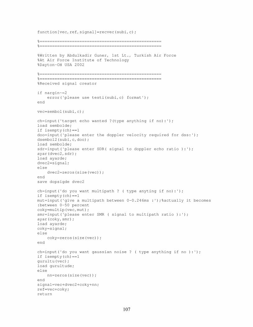
107

function[vec,ref,signal]=recvec(subi,c);

%=================================================%=================================================

%Written by Abdulkadir Guner, 1st Lt., Turkish Air Force%At Air Force Institute of Technology%Dayton-OH USA 2002

%=================================================%=================================================%Received signal creator

if nargin~=2error('please use testi(subi,c) format');

end

vec=sembol(subi,c);

ch=input('target echo wanted ?(type anything if no):');load sembolde;if isempty(ch)==1doo=input('please enter the doppler velocity required for dss:');dsembol2(subi,c,doo);load sembolde;sdr=input('please enter SDR( signal to doppler echo ratio ):');ayar(dvec2,sdr);load ayarde;dvec2=signal;else

dvec2=zeros(size(vec));endsave dopsigde dvec2

ch=input('do you want multipath ? ( type anyting if no):');if isempty(ch)==1mut=input('give a multipath between 0-0.246ms :');%actually it becomes:between 0-50 percentcoky=multip(vec,mut);smr=input('please enter SMR ( signal to multipath ratio ):');ayar(coky,smr);load ayarde;coky=signal;else

coky=zeros(size(vec));end

ch=input('do you want gaussian noise ? ( type anything if no ):');if isempty(ch)==1gurultu(vec);load gurultude;else

nn=zeros(size(vec));endsignal=vec+dvec2+coky+nn;ref=vec+coky;return

108

function[vec]=sembol(subi,c);

%=================================================%=================================================

%Written by Abdulkadir Guner, 1st Lt., Turkish Air Force%At Air Force Institute of Technology%Dayton-OH USA 2002

%=================================================%=================================================%DAB symbol creator

if nargin~=2error('use format sembol(subi,c)');

end

fc = 200000000;totalt = .001;vec=[];freqc=[fc:1000:(subi-1)*1000+fc];freq=freqc-fc+1000;fs=2*max(freq);sample_n=totalt*fs;Fs=2^(3+length(dec2bin(sample_n)));Fc=median(freq)+fc;delta=totalt/Fs;t=[0:delta:totalt-delta];rn=floor(rand(c,subi)*4);save random rnrnn=pi/2*rn;mo=exp(j*rnn);coef=[zeros(c,1) mo zeros(c,Fs-subi-1)];for p=1:c;icoef=real(ifft(coef(p,:)));nicoef=icoef/max(icoef);vec=[vec nicoef];endsave parameter c subi Fs totalt freq tsave semboldsave sembolde vec;return

109

function[]=dsembol2(subi,c,dop);

%=================================================%=================================================

%Written by Abdulkadir Guner, 1st Lt., Turkish Air Force%At Air Force Institute of Technology%Dayton-OH USA 2002

%=================================================%=================================================%Doppler shifted signal creator

if nargin~=3error('use this model:dsembol(subcarrier,symbol,doppler in m/s)');

endfc = 200000000;totalt = .001;dvec2=[];freqc=[fc:1000:(subi-1)*1000+fc];freq=freqc-fc+1000;fs=2*max(freq);sample_n=totalt*fs;Fs=2^(3+length(dec2bin(sample_n)));Fc=median(freq)+fc;

load randomdelta=totalt/Fs;t=[0:delta:totalt-delta];%time vectorfd = 2*dop*Fc/3/10^8;

z=1;for p=1:c;

pt=t+(p-1)*totalt;

for i=1:length(freq);x(z,:)=cos(2*pi*freq(i)*t+(pi/2)*rn(p,i));y(i,:)=cos(2*pi*freq(i)*t+2*pi*fd*pt+(pi/2)*rn(p,i));z=z+1;

enddopp_sigp=sum(y,1);dopp_sigp=dopp_sigp/max(dopp_sigp);dvec2=[dvec2 dopp_sigp];

endsave sembolde dvec2;save nullspace x;return

110

function[]=ayar(signal,snr);

%=================================================%=================================================

%Written by Abdulkadir Guner, 1st Lt., Turkish Air Force%At Air Force Institute of Technology%Dayton-OH USA 2002

%=================================================%=================================================%Signal to noise ratio calculator

if nargin~=2error('use the format ayar(signal,attenuation), at. in dB');endif isempty(snr)==1

ratio=1;else

ratio=10^(snr/10);endsignal=signal/sqrt(ratio);save ayarde signal;return

111

function[mulsig]=multip(sinyal,delay);

%=================================================%=================================================

%Written by Abdulkadir Guner, 1st Lt., Turkish Air Force%At Air Force Institute of Technology%Dayton-OH USA 2002

%=================================================%=================================================%multipath signal creator

if nargin~=2error('enter two parameters:multip(vector,multipath in ms) :1ms

corresponds to 150 km range multipath so be careful \n range between 0to .5ms \n ( if you have an arbitrary signal then this range is 0-.5 ofvectors length');endload parameter;%kk=length(sinyal)/c;mulsig=[];for i=0:c-1;

kak=cokyol(sinyal(1+i*kk:(1+i)*kk),delay);mulsig=[mulsig kak];

endreturn

112

function[xf]=subs(MM);

%=================================================%=================================================

%Written by Abdulkadir Guner, 1st Lt., Turkish Air Force%At Air Force Institute of Technology%Dayton-OH USA 2002

%=================================================%=================================================%subcarrier calculatorload parameterz=1;for p=1:c;

for i=1:length(freq);xf(z,:)=cos(2*pi*freq(i)*t+MM(p,i));z=z+1;end

endreturn

113

function[fiil]=filtre(xf,siglan);

%=================================================%=================================================

%Written by Abdulkadir Guner, 1st Lt., Turkish Air Force%At Air Force Institute of Technology%Dayton-OH USA 2002

%=================================================%=================================================%filtered received signal calculator

load parameter;fiil=[];for i=0:c-1;

I=space3(xf(1+i*subi:(1+i)*subi,:)');filt=I*siglan(1+i*Fs:(1+i)*Fs)';fiil=[fiil filt'];

endreturn

114

function[I]=space3(M);

%=================================================%=================================================

%Written by Abdulkadir Guner, 1st Lt., Turkish Air Force%At Air Force Institute of Technology%Dayton-OH USA 2002

%=================================================%=================================================%filter weights calculator

aa=size(M);if aa(1,1)<aa(1,2)

fprintf('you know that space3 projects into columnsspace of M,right?');endP=M*inv(M'*M)*M';I=eye(length(M))-P;save space3de;return

115

function[axx]=ambfun(x);load sembold;

%=================================================%=================================================

%Written by Abdulkadir Guner, 1st Lt., Turkish Air Force%At Air Force Institute of Technology%Dayton-OH USA 2002

%=================================================%=================================================%detection surface calculator

fdomain=fft([x zeros(1,Fs*c)]);%fdomain contains the fft of the signal

vv=[0:20:400];dopp=length(vv);

delta=totalt/Fs;t=[0:delta:totalt-delta];

axx=zeros(dopp,2*Fs*c);y=zeros(length(freq),length(t));

for b=1:dopp;beta = 1 + 2*vv(b)/3/10^8;factor = 2*vv(b)*fc/3/10^8;dopp_signal=[];

for p=1:c;pt=t+(p-1)*totalt;

for i=1:length(freq);y(i,:)=cos(2*pi*(freq(i)*beta+factor)*pt+(pi/2)*rn(p,i));

enddopp_sigp=sum(y,1);dopp_sigp=dopp_sigp/max(dopp_sigp);dopp_signal=[dopp_signal dopp_sigp];end

dopp_fdomain=fft([zeros(1,Fs*c) dopp_signal]);axx(b,:) = abs(ifft(fdomain.*conj(dopp_fdomain)));

endsave ambfunde;%figure;mesh(linspace(-totalt*c,totalt*c,2*c*Fs)*1000,vv,axx);xlabel('Time [ms]');ylabel('Velocity [m/s]');zlabel('Normalised Ambiguity Function');return

figure;clf;orta=floor(dopp/2+1);

116

if vv(1)==0orta=1;

endnewt=linspace(-totalt*c,totalt*c,length(fdomain));range=150;sampdur=floor(range*2/300000/(newt(2)-newt(1))+1);if sampdur>c*Fs

sampdur=c*Fs;endtstart=length(newt)/2;tstop= length(newt)/2+sampdur;plot(newt(tstart:tstop)*1000,10*log10(axx(orta,tstart:tstop)));xlabel('time in ms');ylabel('the mag of ambiguity funcion for fd=0');title('signal auto correlation for a given range (here 150km) forzerodoppler');

indis=find(xx(orta,:)==max(axx(orta,:)));figure;clf;plot(vv,10*log10(axx(:,indis)));xlabel('relative velocity in m/s');ylabel('the value of ambiguity function for zerotime delay along thedoppler frequencies');title('this plot shows basically how much only-freq-delayed versions ofthe signal look like each other');save cicimdereturn

117

function[]=gurultu(x);

%=================================================%=================================================

%Written by Abdulkadir Guner, 1st Lt., Turkish Air Force%At Air Force Institute of Technology%Dayton-OH USA 2002

%=================================================%=================================================%gaussian noise calculator

randn('state',sum(100*clock));nn=randn(size(x));fprintf('SNR for normalizedcos/nn will be -3 \n');snr=input('how much db SNR increase do you want in SNR ?');if isempty(snr)==1

ratio=1;else

ratio=10^(snr/10);endnn=nn/sqrt(ratio);save gurultude;return

118

BIBLIOGRAPHY

[1] Lesturgie, M., D. Poullin, Frequency allocation in radar: Solutions and compromise for low frequency band, IEEE International Radar Conference 1999, Brest- France.

[2] Willis Nicholas J, Bistatic Radar, Artech House 1991.

[3] Baniak, J., Gregory Baker, Ann Marie Cunningham, Lorraine Martin, Lockheed Martin Mission Systems Silent Sentry™ Passive Surveillance Passive Surveillance, June 7, 1999.

[4] Spaceport News, John F. Kennedy Space Center, August 15, 1997.

[5] Editorial staff, Asia-Pacific report- PRC passive Early warning system, Journal of Electronic Defense, February 2000.

[6] Cazzani, L., Carlo Colesanti, Davide Leva, Giuseppe Nesti, Claudio Prati, Fabio Rocca, Dario Tarchi , A Ground-Based Parasitic SAR Experiment, IEEE transactions on Geoscience and remote sensing,Vol. 38, No. 5, September 2000.

[7] Howland, Paul E., Target tracking using television-based bistatic radar, IEE Proc.-Radar, Sonar, Navig., Vol 146, No. 3, June 1999

[8] Howland, Paul E., Television Based Bistatic Radar, PhD dissertation, School of Electronic and Electrical Engineering University of Birmingham England September 1997.

[9] Sahr, John D., Frank D. Lind, The Manatash Ridge radar: A passive bistatic radar for upper atmospheric radio science, University of Washington, Seattle, preprint URSI 96

[10] Griffiths, H.D., N.R.W. Long, Television based bistatic radar, IEE Proceedings Part F, Vol. 133, No. 7, December 1996

[11] Ringer, M.A., G.J. Frazer, S.J. Anderson, Waveform Analysis of Transmitters of Opportunity for Passive Radar, DSTO Electronics and Surveillance Research Laboratory Salisbury, Australia, June 1999

119

[12] Skolnik, M., Introduction to radar systems, 3rd Edition, McGraw-Hill 2000.

[13] Hoeg, W., T. Lauterbach (editors), Digital Audio Broadcasting Principles and

Applications, John WIley & Son's 2001. [14] ETS (European Telecommunications Standard) 300 401 – Radio Broadcast

Systems, DAB Second Edition, May 1997 [15] Ennes, Harold E., Television Broadcasting : equipment, systems, and operating

fundamentals, W.Sams&Co inc. 1974. [16] Griffiths, H.D., A.J.Garnett, C.J.Baker and S.Keaveney, Bistatic radar using

satellite-born illuminators of opportunity, Proceedings of the IEE International Conference, Radar 92

[17] Vlieger, J.H., R.H.J. Gmelig Meyling, Maximum likelihood estimation for long-

range target tracing using passive sonar measurements, IEEE Transactions On Signal Processing, Vol.40, No.5.

[18] Poullin, D., On the use of COFDM modulation (DAB, DVB) for passive radar

application, Symposium on Passive Radar and LPI(Low Probability of Intercept) Radio Frequency Sensors, NATO RTO, Warsaw, Poland, April 2001.

[19] Kvernsveen, K., H.Ohra, Exploitation of Future Broadcast Transmitters for Radar

Detection and Tracking, Symposium on Passive Radar and LPI(Low Probability of Intercept) Radio Frequency Sensors, NATO RTO, Warsaw, Poland, April 2001.

[20] Van Nee, R., Ramjee Prasad, OFDM for wireless multimedia communications,

Artech House Publishers 2000. [21] Reimers, U., DVB-T: the COFDM-based system for terrestrial television,

Electronics & Communication Engineering Hournal Vol.9, No.1, Feb 1997. [22] Goldberg, Jack L., Matrix theory with applications, McGraw-Hill 1991. [23] Scharf, Louis L., Statistical Signal Processing, Addison-Wesley 1991. [24] Docampo, D., Intelligent methods for signal processing and communication,

Birkhauser 1997. [25] Kay, Steven M., Modern spectral estimation Theory & applications, Prentice-Hall

1988.

120

VITA

First Lieutenant Abdulkadir Guner was born in Istanbul Turkey in 1975. He

entered the Turkish Air Force Academy in 1993 and graduated in 1997 with B.S.E.E.

degree. After graduating from the academy, he entered pilot training and gained F-16

fighter pilot status in July 2000. He was then selected to attend the Air Force Institute of

Technology (AFIT) as a master’s degree student where he studied communications and

radar systems. His research area of interest was passive coherent radar systems. He

graduated from AFIT in March 2002 with an M.S.E.E. degree.

REPORT DOCUMENTATION PAGE Form Approved OMB No. 074-0188

The public reporting burden for this collection of information is estimated to average 1 hour per response, including the time for reviewing instructions, searching existing data sources, gathering and maintaining the data needed, and completing and reviewing the collection of information. Send comments regarding this burden estimate or any other aspect of the collection of information, including suggestions for reducing this burden to Department of Defense, Washington Headquarters Services, Directorate for Information Operations and Reports (0704-0188), 1215 Jefferson Davis Highway, Suite 1204, Arlington, VA 22202-4302. Respondents should be aware that notwithstanding any other provision of law, no person shall be subject to an penalty for failing to comply with a collection of information if it does not display a currently valid OMB control number. PLEASE DO NOT RETURN YOUR FORM TO THE ABOVE ADDRESS. 1. REPORT DATE (DD-MM-YYYY)

15-03-2002 2. REPORT TYPE

Master’s Thesis

3. DATES COVERED (From – To) Jun 2001 – Mar 2002

5a. CONTRACT NUMBER

5b. GRANT NUMBER

4. TITLE AND SUBTITLE AMBIGUITY FUNCTION ANALYSIS AND DIRECT-PATH SIGNAL FILTERING OF THE DIGITAL AUDIO BROADCAST (DAB) WAVEFORM FOR PASSIVE COHERENT LOCATION (PCL)

5c. PROGRAM ELEMENT NUMBER

5d. PROJECT NUMBER 5e. TASK NUMBER

6. AUTHOR(S) Guner, Abdulkadir, 1st Lt., TUAF 5f. WORK UNIT NUMBER

7. PERFORMING ORGANIZATION NAMES(S) AND ADDRESS(S) Air Force Institute of Technology Graduate School of Engineering and Management (AFIT/EN) 2950 P Street, Building 640 WPAFB OH 45433-7765

8. PERFORMING ORGANIZATION REPORT NUMBER AFIT/GE/ENG/02M-09

10. SPONSOR/MONITOR’S ACRONYM(S)

9. SPONSORING/MONITORING AGENCY NAME(S) AND ADDRESS(ES) NATO C3 Agency Attn: Dr. Paul Howland P.O Box174 Telephone No: +31-70 314-2476 Den Haag-The Netherlands e-mail:Paul.Howland@nc3a.nato.int

11. SPONSOR/MONITOR’S REPORT NUMBER(S)

12. DISTRIBUTION/AVAILABILITY STATEMENT APPROVED FOR PUBLIC RELEASE; DISTRIBUTION UNLIMITED.

13. SUPPLEMENTARY NOTES 14. ABSTRACT This research presents an ambiguity function analysis of the digital audio broadcast (DAB) waveform and one signal detection approach based on signal space projection techniques that effectively filters the direct-path signal from the receiver target channel. Currently, most Passive Coherent Location (PCL) research efforts are focused and based on frequency modulated (FM) radio broadcasts and analog television (TV) waveforms. One active area of PCL research includes the search for new waveforms of opportunity that can be exploited for PCL applications. As considered for this research, one possible waveform of opportunity is the European digital radio standard DAB.

For this research, the DAB performance is analyzed for application as a PCL waveform of opportunity. For this analysis, DAB ambiguity function calculations and ambiguity surface plots are created and evaluated. Signal detection capability, to include characterization of time-delay and Doppler-shift measurement accuracy and resolution, is investigated and determined to be quite acceptable for the DAB waveform

15. SUBJECT TERMS Passive Radar, Passive Coherent Location System (PCL), Passive Sensor Location System, Bistatic Radar, Multistatic Radar, Digital Audio Broadcast (DAB), Adaptive Signal Filtering, Coded Orthogonal Frequency Division Multiplex (COFDM)

16. SECURITY CLASSIFICATION OF: 19a. NAME OF RESPONSIBLE PERSON Michael A. Temple, Ph.D.

a. REPORT

U

b. ABSTRACT

U

c. THIS PAGE

U

17. LIMITATION OF ABSTRACT

UU

18. NUMBER OF PAGES

128

19b. TELEPHONE NUMBER (937) 255-3636, ext 4703; e-mail: Michael.Temple@afit.edu

Standard Form 298 (Rev. 8-98) Prescribed by ANSI Std. Z39-18

x