ORIGINAL ARTICLE

Alternative approaches for addressing non-permanencein carbon projects: an application to afforestationand reforestation under the Clean Development Mechanism

Christopher S. Galik & Brian C. Murray &

Stephen Mitchell & Phil Cottle

Received: 14 February 2014 /Accepted: 1 May 2014# Springer Science+Business Media Dordrecht 2014

Abstract Afforestation and reforestation (A/R) projects generate greenhouse gas (GHG)reduction credits by removing carbon dioxide from the atmosphere through biophysicalprocesses and storing it in terrestrial carbon stocks. One feature of A/R activities is thepossibility of non-permanence, in which stored carbon is lost though natural or anthropogenicdisturbances. The risk of non-permanence is currently addressed in Clean DevelopmentMechanism (CDM) A/R projects through temporary carbon credits. To evaluate other ap-proaches to address reversals and their implications for policy and investment decisions, weassess the performance of multiple policy and accounting mechanisms using a forest ecosys-tem simulation model parameterized with observational data on natural disturbances (e.g., fireand wind). Our analysis finds that location, project scale, and system dynamics all affect theperformance of different risk mechanisms. We also find that there is power in risk diversifi-cation. Risk management mechanisms likewise exhibit a range of features and tradeoffs amongrisk conservatism, economic returns, and other factors. Rather than relying on a singleapproach, a menu-based system could be developed to provide entities the flexibility to chooseamong approaches, but care must be taken to avoid issues of adverse selection.

Keywords Afforestation . Carbon . CleanDevelopmentMechanism . Insurance .

Non-permanence . Reforestation . Temporary credit

Mitig Adapt Strateg Glob ChangeDOI 10.1007/s11027-014-9573-4

C. S. Galik (*) : B. C. MurrayNicholas Institute for Environmental Policy Solutions, Duke University, Box 90335,Durham, NC 27708, USAe-mail: csg9@duke.edu

S. MitchellNicholas School of the Environment, Duke University, Durham, NC 27708, USA

P. CottleForestRe Ltd, London, UK EC3N 1LS

1 Introduction: carbon sinks, permanence, and reversals

Land use, land use change, and forestry (LULUCF), which includes agriculture, account forabout one-quarter of global greenhouse gas emissions (Blanco et al 2014). A substantial part ofthis flow is tied to the absorption, storage, and release of carbon dioxide (CO2) in soils,biomass, and other organic pools referred to as carbon sinks. Sinks can accumulate carbonthrough both the maintenance of preexisting stocks (e.g., reduced deforestation, degradation,or other forms of land clearing) or through the creation of new stocks (afforestation, refores-tation, improved management, and other forms of restoration). Terrestrial carbon sequestrationprojects are therefore part of the GHG mitigation strategy set, typically identified as a potentialoffset for emissions from other sources. In principle, using a metric ton of terrestrially storedcarbon (or CO2 equivalent, tCO2e) as an offset is an equivalent credit against an emissionelsewhere if it completely negates the climatic impact of that emission.

Recognizing the importance of terrestrial carbon sinks in climate mitigation, policies havebeen designed and implemented to expand carbon sinks. However, these terrestrial ecosystemsare susceptible to disturbances that cause the stored carbon to be released back into theatmosphere (Brown et al 2000; Dale et al 2001; Galik and Jackson 2009). Problems can arisewhen stored carbon that has been credited as part of a climate change mitigation effort returns tothe atmosphere via these disturbances, a phenomenon known as reversal. Reversals, when theyoccur, can nullify emissions reductions and undermine the permanence of these climate mitiga-tion actions, and so must be otherwise addressed through policies and accounting procedures.

Under the United Nations Framework Convention on Climate Change Kyoto Protocol’sClean DevelopmentMechanism (CDM), developing countries can host carbon sink projects thatgenerate certified emission reduction credits. These credits can be sold to developed (Annex I)countries to help them meet their emissions reduction obligations. Currently, CDM afforestationand reforestation (A/R) projects address reversals by issuing expiring (temporary) credits. Uponexpiration, these credits must be replaced. This replacement requirement raises the cost to thebuyer of using them relative to a full-price permanent credit, thereby reducing the monetaryvalue of the credit and the net revenue flow to the project (Olschewski and Benítez 2005).

As A/R projects have not been widely adopted thus far—they account for less than onepercent of all CDM projects to date (United Nations Environment Programme UNEP 2012)—the question is whether other approaches for dealing with reversals are needed and how theperformance of these approaches varies as applied. Here we assess non-permanence risk in A/R project-level activities under multiple policy approaches. Using the LANDCARB forestecosystem simulation model (Harmon 2012), we investigate the influence of policy choice inthe presence of random natural disturbance events on the long-term financial and environ-mental viability of project-based offsets. We quantify the performance of different reversal riskapproaches under the threat of both wildfire and wind disturbance project on a hypotheticalsubtropical project representative of A/R project experience under the CDM (see, e.g., CleanDevelopment Mechanism CDM 2012). In doing so, we provide an example of how large-scalemodels may be employed for evaluation of project-level accounting decisions to informongoing discussions of both CDM and emerging compliance and voluntary market activities.

2 Reversal risk: types and characteristics

LULUCF activities are subject to both natural and anthropogenic disturbances. Relevantnatural disturbances include fire, wind, flood, drought, ice/snow, pest infestations, disease,landslides, earthquakes, and volcanic activity (see Galik and Jackson 2009 for a review).

Mitig Adapt Strateg Glob Change

Human-induced disturbances include the legal or illegal harvesting of trees, land clearing, andincidental mortality occurring as a result of other activities (e.g., war). The intensity and extentof disturbance can vary for both human-caused and natural events, ranging from slight damageto complete loss and from individual trees to thousands of hectares.

Risks to LULUCF activity may be classified into two types: (1) unintentional reversals dueto natural disturbances outside of the project holder’s control (such as wildfires, wind, andflooding) and (2) intentional risks caused by purposeful actions of the project holder (such asharvesting, land clearing, and intentionally set fires). For the purposes of the empirical analysispresented here, we consider only unintentional (natural) reversals. This is not to diminish theimportance or relevance of intentional reversals, but recognizes that the suite of approaches toaddress intentional reversals are potentially different from those best used in unintentionalreversals. Intentional reversals, for example, may be more easily traced back to responsibleparties, thus facilitating repayment through contractual obligations or other legal means.Unintentional reversals, however, involve loss from stochastic, force majeure events for whichthere may be no responsible entity, requiring that the approaches used to ensure systemintegrity be evaluated and well understood.

Wildfire and wind are common causes of natural, unintentional loss, but a great deal of variationexists both within and between each with regard to disturbance frequency, intensity, and areaaffected (see, e.g., Dale et al 2001). Low-intensity fires may affect large areas but consume onlylitter and ground vegetation, resulting in negligible carbon consequences for an A/R project.Conversely, high-intensity fires can reach into the forest crown and be utterly destructive, withcatastrophic results for both previously stored carbon and future sequestration potential. Wind,meanwhile, tends to affect small areas but with great intensity. While the blow-down that resultsfrom severe wind events may kill or damage individual trees, stored carbon may not be lostimmediately but rather transferred from live tree to dead tree pools where it is lost slowly over time.

3 Risk management approaches: concepts and criteria

Selection of a reversal risk management approach requires multiple determinations. Each stageof the approach selection process likewise involves multiple considerations. Beginning with adetermination of who is ultimately liable for reversals should they occur, decisions also need tobe made on whether awarded credits are temporary or permanent, and whether full credits areissued or whether they are awarded incrementally over time.

3.1 Liability determination and assignment

A necessary first step is to assign liability for reversals. From an accounting perspective, a reversaloccurs once it is detected, quantified, and reported. Standard practice would cancel creditsequivalent to the size of the reversal. Since canceled credits mean that the use of the credits foroffsetting emissions has been compromised, some replacement of the canceled credits with validcredits would be necessary to restore balance to the system. The issue comes down to who isliable for replacing the credits. Although largely a policy determination, the assignment ofliability can itself determine the incentives to manage for the reduction in non-permanence risk.

3.2 Accounting mechanisms for addressing reversals as they occur

The incidence of reversal can be automatically incorporated into the crediting system in anumber of ways. Historically, many of the considerations for addressing reversals have

Mitig Adapt Strateg Glob Change

evolved from a project-level perspective and emerged from the modalities and proceduresdeveloped for A/R under the CDM and from the voluntary market. Although often lumpedtogether as ways to collectively address non-permanence, the following approaches arefundamentally different in the questions they seek to answer and the function they seek toprovide.

3.2.1 Incremental crediting over time

One could assign more permanent credits for projects that store carbon for longer periods oftime. One such approach is the tonne year approach (Moura-Costa and Wilson 2000; Nobleet al 2000), which is similar in some ways to the rental approach described by Sohngen (2003)in which credits accrue the longer the carbon is stored. In this approach, tonnes stored early onin a project receive small payments that progressively accumulate as the project continues andachieves storage over a longer period. Because payments are based on achieved permanence,there is no up-front payment for permanent credits once initial storage is verified and noliability to replace the credit if reversal occurs. Rather, a reversal simply reduces the basis forsubsequent payments.

3.2.2 Full crediting upon verification

Rather than awarding credits incrementally, credits could be fully awarded upon verification.Doing so, however, requires that mechanisms be in place to ensure that any carbon that issubsequently lost to reversal is somehow accounted for or replaced. Under the temporarycertified emission reduction (tCER) approach of the CDM, all credits that were issued for aproject expire at the end of the (Kyoto Protocol) commitment period after they were issued.The tCERs can however be reissued upon subsequent verification. Crediting periods can bemuch longer for long-term certified emission reductions (lCERs), which are valid for20 years, renewable twice (for up to 60 years) or for a single, 30-year crediting period.Simple economics suggests that the difference in credit life will translate into a difference inprice between the two types of credits. Under a system that mandates replacement at the endof the contracts, short contracts will have heavily discounted credits, since the replacementrequirement will be near at hand (Kim et al 2008; Murray et al 2007). lCERs would thereforecommand a higher price than tCERs due to the greater amount of time before replacement isrequired, while themselves trading for less than a comparable permanent credit. While longercontracts should have lower discounts, there is no transaction data upon which to confirmthis.

An alternative is to issue fungible permanent credits once carbon storage is verified,typically requiring replacement of credits previously issued for carbon that has been deemedto have been reversed before the end of the period stipulated to fulfill a permanence obligation.These credits can be sold as soon as the carbon is sequestered and credits are issued. But as thecredit is issued prior to fully serving its offsetting function, and with no preset expectation ofexpiration as in the case of temporary credits, legal obligations to replace lost storage and/orspecific accounting procedures to facilitate such replacement are typically put in place toensure that system integrity is not affected by a reversal.

One mechanism to ensure replacement of lost storage is to require the creation of a buffer orset-aside. The buffer concept is common in the voluntary market. It has also caught hold in theUNFCCC process, as evidenced by CMP7 approved modalities and procedures for geologicalcarbon capture and storage (CCS) projects under the CDM (UNFCCC 2011b). A bufferapproach requires that some portion of earned credits be set aside or held in escrow to address

Mitig Adapt Strateg Glob Change

non-permanence. If a reversal occurs under the buffer approach, credits from the buffer areused to compensate for the carbon storage lost. The size of the set aside may vary dependingon the inherent riskiness of the activity and the length of time over which the risk is evaluated(Verified Carbon Standard VCS 2012).

Another way to address the potential loss of permanent credits is through commercialinsurance. Private insurance for carbon markets and policy regimes functions much the sameas it does in personal service and commodity markets. Regular payments, or premiums, arepaid to some insuring entity, which in turn guarantees the permanence of credits generated bythe covered activity (e.g., by replacing reversed credits). In the event of loss, the project willlikely be required to first pay a deductible. As opposed to buffers, which require that somenumber of credits be set aside up front, the deductible is an “if and when” call that is onlyrequired upon reversal. Although carbon insurance products are rare now, analogs exist inother forest and agriculture applications. When it is available, a primary benefit of insurance isthat it is simple and straightforward to implement so long as the insuring entity is appropriatelycapitalized to withstand catastrophic loss.

A project’s host country could agree to replace any credits lost to reversal. Such a guaranteewould allow projects to be marketed at lower risk to the buyer, thereby increasing creditdemand. The host country guarantee approach builds off recent proposals to address residualliability for carbon, capture and storage (CCS) activities under the CDM (UNFCCC 2011b), inwhich the host country acts as a fiduciary backstop to address reversals from physical leakage ofCO2 from the storage reservoir unresolved at the project or sub-national level. Precedent alsoexists under the Joint Implementation (JI) mechanism of the Kyoto Protocol, in which projectlosses must be balanced against a given country’s national account. Under this model, a givencountry or their designated third party can choose to assume liability for any losses over andabove the provisions made for covering losses (such as a buffer) at the project or sub-nationalprogram levels. The economic viability of such an approach depends on the relationshipbetween the monetary value of expected losses and host country or third-party willingnessand ability to devote the necessary resources to cover them.

Finally, it is possible to have a replacement obligation in the absence of any formal mechanism(i.e., no buffer contribution/commercial insurance coverage requirement). With no mechanismfacilitating credit payback, however, protections must be put into place to ensure that affectedprojects have the financial resources to compensate for lost storage. One way to do this is torequire a project to establish a performance bond or some other form of collateral in advance.

4 Quantitative analysis of risk management approaches

4.1 Simulation of growth and disturbance

We simulated forest growth using a significantly updated version of the ecosystem simulationmodel LANDCARB (Harmon 2012). LANDCARB is a landscape-level ecosystem processmodel. LANDCARB integrates climate-driven growth and decomposition processes withspecies-specific rates of senescence and mortality, while incorporating the dynamics of inter-and intra-specific competition that characterize forest gap dynamics. Inter- and intra-specificcompetition dynamics are accounted for by modeling species-specific responses to solarradiation as a function of each species’ light compensation point and assuming light isdelineated through foliage following a Beer-Lambert function. By incorporating these dynam-ics, the model simulates successional changes as one life-form replaces another, therebyrepresenting the associated changes in ecosystem processes that result from species-specific

Mitig Adapt Strateg Glob Change

rates of growth, senescence, mortality, and decomposition. LANDCARB represents stands ona cell-by-cell basis, with the aggregated matrix of stand cells representing an entire landscape.Each cell in LANDCARB simulates a number of cohorts that represent different episodes ofdisturbance and colonization within a stand. Each cohort contains up to four layers ofvegetation (upper tree layer, lower tree layer, shrub, and herb).

To generate a distribution of results for each risk management approach, we re-run themodel 50 times under the threat of random fire and wind disturbance. For each of the 50 runsperformed for each scenario, we assessed a 45×45 matrix of 10 hectare cells, for a total projectarea of 20,250 ha. To assess forest growth and disturbance on the performance of smallerprojects, we randomly selected a starting cell from each run of 45×45 cells and chose theadjacent 10 rows and columns, yielding a smaller project area of 1,000 ha. For all projects, weassume that lands are afforested in the first year of the project. No harvests are conductedduring the project, meaning that we do not track harvested wood products (HWP) nor do weassess potential long-term carbon storage in the HWP pool.

Forest growth in our model runs is based on growth-yield curves established for highmanagement, high productivity softwood plantation species (Pinus taeda-P. echinata) standsas described in Smith et al (2006). These and other similar softwood species are featured inexisting A/R projects. The sequestration profile of P. taeda also lies between faster growingshorter rotation species and slower growing longer rotation species used in A/R projects(Fig. 1), thus providing for a rough mid-point analysis.

Our analysis incorporates wildfires in all simulations. In the LANDCARB model, fireseverity controls the amount of live vegetation killed and the amount of combustion from thevarious C pools, and is influenced by the amount and type of fuel present. Fires can increase(or decrease) in severity depending on how much the weighted fuel index of a given cellexceeds (or falls short of) the fuel level thresholds for each fire severity class (Tlight, Tmedium,

Fig. 1 Sequestration profile for species used (or equivalent) in CDM A/R projects. Pinus taeda (U.S.) shows thesequestration profile of the forest type assumed in the quantitative analysis performed in this paper. Source: CostaRica Tectona grandis – Bermejo et al (2004), site index 23, fit using simple polynomial trendline; T.grandis,Eucalyptus tereticornis, and Populus deltoids (India) – Kaul et al (2010); P. taeda (U.S.) – adapted from Smithet al (2006); P. radiata – Paul et al (2008)

Mitig Adapt Strateg Glob Change

Thigh, and Tmax) and the probability values for the increase or decrease in fire severity (Pi andPd). For example, a low-severity fire may increase to a medium-severity fire if the fuel indexsufficiently exceeds the threshold for a medium-severity fire. Fuel-level thresholds were set bymonitoring fuel levels in a large series of simulation runs where fires were set at very shortintervals to see how low fuel levels needed to be to create a significant decrease in expectedfire severity.

The modeled fire regime is intended to replicate fire behavior in subtropical loblolly pinestands. Not only does this fire regime conform to our choice of species to use in the A/Rproject, but it may also be representative of other subtropical locations that are home to asizable portion of current A/R projects. Although data on low-frequency, high-severity fires isgenerally unavailable in the Southeastern U.S. due to a lack of primary forest on which firereconstruction studies could be performed, we can nonetheless estimate reasonable fire returnintervals through comparison with other forested systems. For example, longleaf pine standsare adapted to a low-severity, high-frequency (3–7 years) fire regime; loblolly pine stands burnwith less frequency than longleaf pine stands, but this is, in part, due to fire suppression. Basedon the observed frequencies in other systems, we thus estimate a reasonable mean fire returninterval (MFRI) in the system modeled here to be 16 years for a low-severity burn, a 100-yearMFRI for a medium-severity fire, and a 300-year MFRI for a high-severity fire. From these,we generated exponential random variables to assign the years of fire occurrence (Van Wagner1978). Fire severities in each year generated by this function are cell-specific, as each cell isassigned a weighted fuel index calculated from fuel accumulation within that cell and therespective flammability of each fuel component, the latter of which is derived from estimatesof wildfire-caused biomass consumption.

Wind loss is represented in the LANDCARB model as a harvest in which no timber isremoved (i.e., all downed timber is left onsite). Lacking adequate data on the distribution ofwind disturbance frequency and intensity in any of the countries currently hosting A/Rprojects, we used U.S. data as a proxy. The incidence and intensity of wind disturbance eventswere derived from the National Oceanic and Atmospheric Administration (NOAA) NationalClimatic Data Center Storm Events Database,1 using the state of Georgia, USA, as a referencepoint. Area affected is not consistently included in the events database, so we instead used U.S.census data on housing density and housing value along with expected levels of damage atvarying wind intensities as reported in the Fujita tornado damage scale, to generate estimatesof windstorm area.2 Next, we estimated likely loss to a forested stand and assumed that allevents of a particular intensity resulted in a particular loss of forest overstory. Events above 45meters per second (m/s, or approximately 100 mph) resulted in 100-percent loss, 35–45 m/s(approximately 78–100 mph) resulted in 75-percent loss, and 25–35 m/s (approximately 56–78 mph) result in 50-percent loss.3 When this exercise was conducted for Clayton County,Georgia, an area slightly larger (37,037 ha) than our modeled landscape area (20,250 ha), weestimated that the average annual percent area affected is 0.3 %, with an average weightedintensity of 50 % loss. This average annual loss was applied to the modeled scenario each year,but its spatial occurrence was randomized (i.e., 0.3 % of the area will be affected each year, butwhere it occurs will be randomly assigned by the model).

1 http://www.ncdc.noaa.gov/stormevents/ftp.jsp Cited 6 August 6 2012.2 http://www.spc.noaa.gov/faq/tornado/f-scale.html Cited 6 August 2012.3 Thresholds are based on categories and descriptions of loss detailed on pp 350–1 in Mason (2002), though theassignment of loss percentages to each threshold is ours alone. Assessing the risk of wind damage is acomplicated undertaking, and we acknowledge this treatment vastly oversimplifies the effect of winddisturbance on forest stands. See, e.g., Quine (1995), Moore and Quine (2000), and Mason (2002) for moreinformation.

Mitig Adapt Strateg Glob Change

Our model results provide an indication of possible losses under a specific set of parametersand assumptions, but use of a different forest type or different disturbance regime is likely togenerate different output data on both carbon storage and the susceptibility of that storage tosubsequent loss. Slow-growing hardwoods in fire-prone tropical and subtropical broadleafforest ecosystems would encounter wildfire and be affected by fire differently than, say, atemperate softwood plantation. Nonetheless, the analysis presented here is broadly informativein comparing different approaches to addressing non-permanence under representative cir-cumstances. This can provide a platform for future work that encompasses more geographicand risk conditions.

4.2 Modeling of risk management approaches

Having first generated raw output data on forest condition under the threat of wind and fire, wethen employ a modified forest offset accounting framework (e.g., Galik and Cooley 2012) totrack the environmental and financial performance of the hypothetical project under severalrisk management approaches. For each LANDCARB run and risk management approach, wetrack the costs associated with A/R project establishment and implementation, the revenuesgenerated by the sale of stored carbon, and the carbon consequences of reversal events. Projectassumptions and cost data used for all policy scenarios are included in Table 1. For tonne yearscenarios, we further assumed a 40 year permanence period. The permanence period definesthe fraction of the credit earned in each year. The 40-year permanence period assumed heremeans that 2.5 % (100 %/40) of a credit will be earned in any given year, which is then sold atthe estimated carbon price for that year. For buffer scenarios, 10 % of net additional carbonstorage in a given year is placed into a set-aside pool; the remaining carbon generated in thatyear is then sold at the estimated carbon price.

The calculation of tCER pricing is more complicated, as the value of a temporary creditstems from the deferred compliance the credit generates. An entity that purchases a tCERoffsets full compliance by the number of years the tCER stands viable. Short contracts willhave heavily discounted credits, since the replacement requirement will be near at hand (Kimet al 2008; Murray et al 2007). Longer contracts should have lower discounts, but this dependson the expectation of future prices for replacement credits; if the price of replacement credits isexpected to be much higher in the future than it is today, then temporary credits may have littlevalue. For tCECRs to maintain any value, prices of permanent credit must grow at a rate lowerthan the discount rate (Olschewski and Benítez 2005; Maréchal and Hecq 2006; Bird et al2004; Subak 2003). If the rate of growth of permanent credits is equal to or greater than thediscount rate, however, the value of a temporary credit becomes zero or negative.

At assumed carbon price increase rates and global discount rates (assumed in this analysisto both be 6 %), the theoretical price of tCERs goes to $0. There is no market transactionhistory, however, to confirm the relevance of the theoretical value of tCERs to actual trades.The only trades in tCERs of which we are aware are recent purchases by the BioCarbon Fundfor approximately $4–5/tCO2e.

4 As these purchases are better viewed as an attempt to seed anascent market, the question remains as to the true value of a tCER. A price $0 is obviously toolow a price to fairly assess the net present value (NPV) of a tCER approach—but $4 is likelytoo high. Accordingly, we instead rely on general relationships noted in Bird et al (2004). Insituations where the discount rate and “inflation rate” (assumed to be the rate of carbon priceincrease) are similar in value, 5-year tCERs will trade at approximately 10 % of the price of

4 See the following CDM project descriptions: http://cdm.unfccc.int/Projects/DB/JACO1260322827.04/viewand http://cdm.unfccc.int/Projects/DB/JACO1245724331.7/view Cited 15 February 2012.

Mitig Adapt Strateg Glob Change

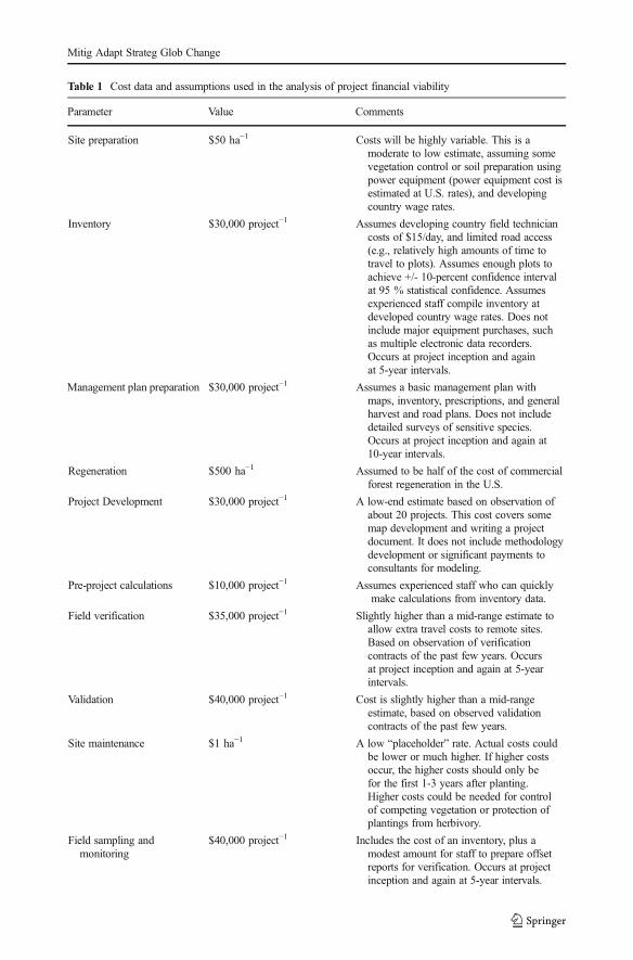
Table 1 Cost data and assumptions used in the analysis of project financial viability

Parameter Value Comments

Site preparation $50 ha−1 Costs will be highly variable. This is amoderate to low estimate, assuming somevegetation control or soil preparation usingpower equipment (power equipment cost isestimated at U.S. rates), and developingcountry wage rates.

Inventory $30,000 project−1 Assumes developing country field techniciancosts of $15/day, and limited road access(e.g., relatively high amounts of time totravel to plots). Assumes enough plots toachieve +/- 10-percent confidence intervalat 95 % statistical confidence. Assumesexperienced staff compile inventory atdeveloped country wage rates. Does notinclude major equipment purchases, suchas multiple electronic data recorders.Occurs at project inception and againat 5-year intervals.

Management plan preparation $30,000 project−1 Assumes a basic management plan withmaps, inventory, prescriptions, and generalharvest and road plans. Does not includedetailed surveys of sensitive species.Occurs at project inception and again at10-year intervals.

Regeneration $500 ha−1 Assumed to be half of the cost of commercialforest regeneration in the U.S.

Project Development $30,000 project−1 A low-end estimate based on observation ofabout 20 projects. This cost covers somemap development and writing a projectdocument. It does not include methodologydevelopment or significant payments toconsultants for modeling.

Pre-project calculations $10,000 project−1 Assumes experienced staff who can quicklymake calculations from inventory data.

Field verification $35,000 project−1 Slightly higher than a mid-range estimate toallow extra travel costs to remote sites.Based on observation of verificationcontracts of the past few years. Occursat project inception and again at 5-yearintervals.

Validation $40,000 project−1 Cost is slightly higher than a mid-rangeestimate, based on observed validationcontracts of the past few years.

Site maintenance $1 ha−1 A low “placeholder” rate. Actual costs couldbe lower or much higher. If higher costsoccur, the higher costs should only befor the first 1-3 years after planting.Higher costs could be needed for controlof competing vegetation or protection ofplantings from herbivory.

Field sampling andmonitoring

$40,000 project−1 Includes the cost of an inventory, plus amodest amount for staff to prepare offsetreports for verification. Occurs at projectinception and again at 5-year intervals.

Mitig Adapt Strateg Glob Change

full permanent credits, the relationship assumed here. At the end of every 5-year projectperiod, total project carbon storage is therefore sold at this carbon price.

Finally, we explore three private insurance options: project full value replacement, cata-strophic loss limit, and buffer insurance. Project full value guarantees replacement of all lossesfrom a project due to a variety of disturbances. Catastrophic loss limit covers up to the amountexpected to be lost in a rare, catastrophic disturbance event (e.g., a 1-in-250 year event). Bufferinsurance, meanwhile, guarantees capitalization up to a certain threshold of a given buffer(e.g., 85 % of initial buffer volume), providing a commercial insurance backstop againstexcessive buffer depletion.

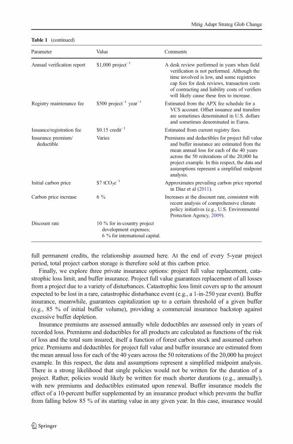
Insurance premiums are assessed annually while deductibles are assessed only in years ofrecorded loss. Premiums and deductibles for all products are calculated as functions of the riskof loss and the total sum insured, itself a function of forest carbon stock and assumed carbonprice. Premiums and deductibles for project full value and buffer insurance are estimated fromthe mean annual loss for each of the 40 years across the 50 reiterations of the 20,000 ha projectexample. In this respect, the data and assumptions represent a simplified midpoint analysis.There is a strong likelihood that single policies would not be written for the duration of aproject. Rather, policies would likely be written for much shorter durations (e.g., annually),with new premiums and deductibles estimated upon renewal. Buffer insurance models theeffect of a 10-percent buffer supplemented by an insurance product which prevents the bufferfrom falling below 85 % of its starting value in any given year. In this case, insurance would

Table 1 (continued)

Parameter Value Comments

Annual verification report $1,000 project−1 A desk review performed in years when fieldverification is not performed. Although thetime involved is low, and some registriescap fees for desk reviews, transaction costsof contracting and liability costs of verifierswill likely cause these fees to increase.

Registry maintenance fee $500 project−1 year−1 Estimated from the APX fee schedule for aVCS account. Offset issuance and transfersare sometimes denominated in U.S. dollarsand sometimes denominated in Euros.

Issuance/registration fee $0.15 credit−1 Estimated from current registry fees.

Insurance premium/deductible

Varies Premiums and deductibles for project full valueand buffer insurance are estimated from themean annual loss for each of the 40 yearsacross the 50 reiterations of the 20,000 haproject example. In this respect, the data andassumptions represent a simplified midpointanalysis.

Initial carbon price $7 tCO2e−1 Approximates prevailing carbon price reported

in Diaz et al (2011).

Carbon price increase 6 % Increases at the discount rate, consistent withrecent analysis of comprehensive climatepolicy initiatives (e.g., U.S. EnvironmentalProtection Agency, 2009).

Discount rate 10 % for in-country projectdevelopment expenses;6 % for international capital.

Mitig Adapt Strateg Glob Change

seek only to address the incremental natural disturbance events that would otherwise depletethe buffer over time. Our modeling resulted in so few years of buffer failure that pricing aproduct that simply insures against collapse was not possible using standard techniques. Insituations of low probability loss, we instead priced premiums on a rate on line (ROL) basis, orthe percentage that the premium bears to the insurers’ totally liability (typically 3 to 4 %).

4.3 Results

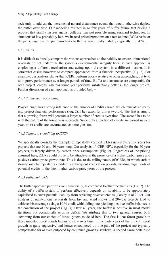
It is difficult to directly compare the various approaches on their ability to ensure unintentionalreversals do not undermine the system’s environmental integrity because each approach isemploying a different mechanism and acting upon the system in a different manner. It issomewhat easier, however, to compare approaches from a financial perspective (Fig. 2). Forexample, our analysis shows that tCERs perform poorly relative to other approaches, but tendto improve performance over longer periods of time. Buffer and insurance are comparable forboth project lengths, whereas tonne year performs substantially better in the longer project.Further discussion of each approach is provided below.

4.3.1 Tonne year accounting

Project length has a strong influence on the number of credits earned, which translates directlyinto project financial performance (Fig. 2). The reason for this is twofold. The first is simplythat a growing forest will generate a larger number of credits over time. The second has to dowith the nature of the tonne year approach. Since only a fraction of credits are earned in eachyear, more credits are accumulated as time goes on.

4.3.2 Temporary crediting (tCERS)

We specifically consider the example of repeatedly verified tCERs issued every five years forprojects that are 20 and 40 years long. Our analysis of tCER NPV, especially for the 40-yearprojects, is largely driven by carbon price assumptions (Fig. 2). Regardless of the pricingassumed here, tCERs could prove to be attractive in the presence of a higher carbon price andpositive carbon price growth rate. This is due to the rolling nature of tCERs, in which carbonstorage may be repeatedly credited in subsequent verification periods, yielding large pools ofpotential credits in the later, higher-carbon-price years of the project.

4.3.3 Buffer set aside

The buffer approach performs well, financially, as compared to other mechanisms (Fig. 2). Theability of a buffer system to perform effectively depends on its ability to be appropriatelycapitalized to cover potential liability from replacing reversed credits (Cooley et al 2012). Ouranalysis of unintentional reversals from fire and wind shows that 20-year projects tend toachieve this coverage using a 10 % credit withholding rate, yielding positive buffer balances atthe conclusion of the project (Fig. 3). Over 40 years, the buffer is positive in most modeliterations but occasionally ends in deficit. We attribute this to two general causes, bothstemming from our choice of forest system modeled here. The first is that forest growth inthese modeled forest stands begins to slow over time. In the early years of the project, forestgrowth is quite aggressive and losses encountered on one part of the project are typicallycompensated for or even outpaced by continued growth elsewhere. A second cause pertains to

Mitig Adapt Strateg Glob Change

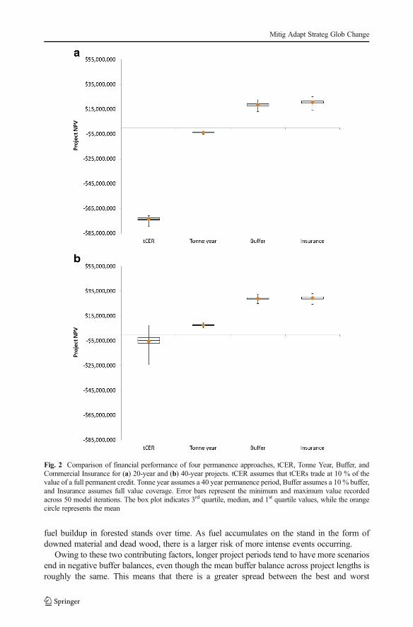
fuel buildup in forested stands over time. As fuel accumulates on the stand in the form ofdowned material and dead wood, there is a larger risk of more intense events occurring.

Owing to these two contributing factors, longer project periods tend to have more scenariosend in negative buffer balances, even though the mean buffer balance across project lengths isroughly the same. This means that there is a greater spread between the best and worst

Fig. 2 Comparison of financial performance of four permanence approaches, tCER, Tonne Year, Buffer, andCommercial Insurance for (a) 20-year and (b) 40-year projects. tCER assumes that tCERs trade at 10 % of thevalue of a full permanent credit. Tonne year assumes a 40 year permanence period, Buffer assumes a 10 % buffer,and Insurance assumes full value coverage. Error bars represent the minimum and maximum value recordedacross 50 model iterations. The box plot indicates 3rd quartile, median, and 1st quartile values, while the orangecircle represents the mean

Mitig Adapt Strateg Glob Change

performing projects over time. Increasing buffer withholding rates can reduce or eliminateinstances of negative buffers in the scenarios modeled here, but this comes at a financial cost tothe project and fails to address the increasing spread between project outcomes.

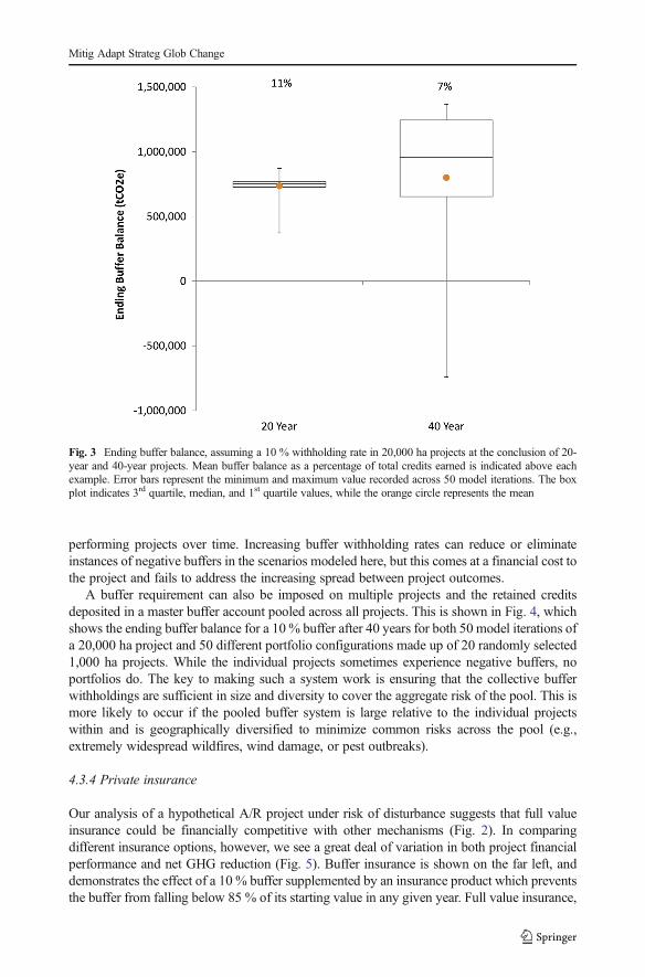
A buffer requirement can also be imposed on multiple projects and the retained creditsdeposited in a master buffer account pooled across all projects. This is shown in Fig. 4, whichshows the ending buffer balance for a 10 % buffer after 40 years for both 50 model iterations ofa 20,000 ha project and 50 different portfolio configurations made up of 20 randomly selected1,000 ha projects. While the individual projects sometimes experience negative buffers, noportfolios do. The key to making such a system work is ensuring that the collective bufferwithholdings are sufficient in size and diversity to cover the aggregate risk of the pool. This ismore likely to occur if the pooled buffer system is large relative to the individual projectswithin and is geographically diversified to minimize common risks across the pool (e.g.,extremely widespread wildfires, wind damage, or pest outbreaks).

4.3.4 Private insurance

Our analysis of a hypothetical A/R project under risk of disturbance suggests that full valueinsurance could be financially competitive with other mechanisms (Fig. 2). In comparingdifferent insurance options, however, we see a great deal of variation in both project financialperformance and net GHG reduction (Fig. 5). Buffer insurance is shown on the far left, anddemonstrates the effect of a 10 % buffer supplemented by an insurance product which preventsthe buffer from falling below 85 % of its starting value in any given year. Full value insurance,

Fig. 3 Ending buffer balance, assuming a 10 % withholding rate in 20,000 ha projects at the conclusion of 20-year and 40-year projects. Mean buffer balance as a percentage of total credits earned is indicated above eachexample. Error bars represent the minimum and maximum value recorded across 50 model iterations. The boxplot indicates 3rd quartile, median, and 1st quartile values, while the orange circle represents the mean

Mitig Adapt Strateg Glob Change

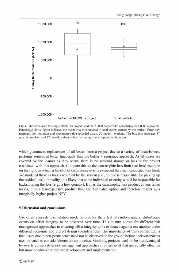
which guarantees replacement of all losses from a project due to a variety of disturbances,performs somewhat better financially than the buffer + insurance approach. As all losses arecovered by the insurer as they occur, there is no residual storage or loss to the projectassociated with this approach. Compare this to the catastrophic loss limit (cat loss) exampleon the right, in which a handful of disturbance events exceeded the mean calculated loss limit.We modeled these as losses recorded by the system (i.e., no one is responsible for picking upthe residual loss). In reality, it is likely that some individual or entity would be responsible forbackstopping the loss (e.g., a host country). But as the catastrophic loss product covers fewerlosses, it is a less-expensive product than the full value option and therefore results in amarginally higher project NPV.

5 Discussion and conclusions

Use of an ecosystem simulation model allows for the effect of random natural disturbanceevents on offset integrity to be observed over time. This in turn allows for different riskmanagement approaches to ensuring offset integrity to be evaluated against one another underdifferent economic and project design considerations. The importance of this contribution isthat losses due to non-permanence need not be observed on the ground before decision-makersare motivated to consider alternative approaches. Similarly, projects need not be disadvantagedby overly conservative risk management approaches if others exist that are equally effectivebut more conducive to project development and implementation.

Fig. 4 Buffer balance for single 20,000 ha projects and the 20,000 ha portfolio comprising 20 1,000 ha projects.Percentage above figure indicates the mean loss as compared to total credits earned by the project. Error barsrepresent the minimum and maximum value recorded across 50 model iterations. The box plot indicates 3rd

quartile, median, and 1st quartile values, while the orange circle represents the mean

Mitig Adapt Strateg Glob Change

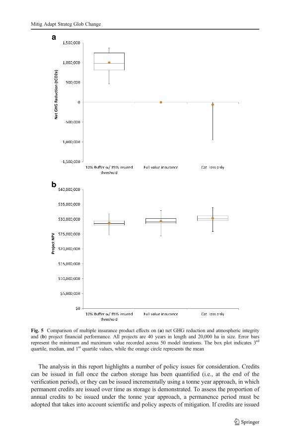
The analysis in this report highlights a number of policy issues for consideration. Creditscan be issued in full once the carbon storage has been quantified (i.e., at the end of theverification period), or they can be issued incrementally using a tonne year approach, in whichpermanent credits are issued over time as storage is demonstrated. To assess the proportion ofannual credits to be issued under the tonne year approach, a permanence period must beadopted that takes into account scientific and policy aspects of mitigation. If credits are issued

Fig. 5 Comparison of multiple insurance product effects on (a) net GHG reduction and atmospheric integrityand (b) project financial performance. All projects are 40 years in length and 20,000 ha in size. Error barsrepresent the minimum and maximum value recorded across 50 model iterations. The box plot indicates 3rd

quartile, median, and 1st quartile values, while the orange circle represents the mean

Mitig Adapt Strateg Glob Change

in full at the time of verification, this leads to the issue of whether those credits are temporarycredits with an expiry date, as is currently the case with CDM A/R credits, or whether they arepermanent credits on par with credits from other sectors under the CDM and other complianceand voluntary markets.

If temporary crediting is pursued, subsequent decisions are necessary to determine whetherto continue with existing practices—tCERS and lCERs with full replacement required atdefined points in time—or to modify the approach slightly, perhaps altering length ofcommitment or credit periods. For permanent credits issued upon verification, there arerequirements to both identify the reversal management approach to be used (buffer/insur-ance/host country guarantee) and to clarify contingent liability for credit replacement uponreversal (project/seller or buyer). The point in time at which point storage has reached anacceptable level of permanence must also be clarified in order to assess replacement liability,particularly in the case of a tonne year approach. The choice of approach is therefore not theonly consideration that must be weighed; the assignment of liability and the permanenceperiod likewise have implications for the environmental integrity and financial viability of A/Rprojects.

Focusing on the selection of reversal risk approaches, our analysis presents the variousaccounting approaches as being separate and apart from one another, but program rules couldbe set up in to combine features of the different accounting approaches discussed above intoone system. For example, one could have temporary crediting with only partial replacement atexpiry, based on interim permanence achieved via the tonne year principles or a programmaticbuffer backed by commercial insurance or host country guarantee in the event of buffer failure.Alternatively, a menu-based system could be set up to allow entities the flexibility to chooseamong approaches; the menu-based approach could also be useful given different countries’capacities for guarantees. Some options have lower initial financial returns, but they reduceobligations for long-term commitment and thus might suit some project participants better assuch provisions would allow them to more easily opt out should circumstances warrant. Otherparties may be more willing to commit to longer time periods and opt to generate permanentcredits upon verification, but also accept the responsibilities associated with replacement underdifferent options presented to them – system buffer or commercial insurance (if available),possibly backed up by a financial guarantee on the part of the project participants or someother third party.

In establishing options, particularly if allowing entities to choose their preferred approach,care must be taken to avoid issues of adverse selection. This could occur, for example, if high-risk projects, unable to secure coverage or competitive rates for private insurance, turn insteadto a managed buffer system. In such a case, the composition of the resulting buffer would beskewed by contributions from these higher-risk projects, making it more likely to be drawnupon and, therefore, more prone to failure.

Although this analysis was initially motivated by discussions under the UNFCCC toconsider alternative approaches for addressing the risk of non-permanence under the CDM(UNFCCC 2011a), it presents information relevant to existing voluntary markets and emergingcountry- or state- level compliance markets. It presents an approach for evaluating the effectsof stochastic disturbance events on the financial and environmental viability of biologicaloffset projects under different policy approaches. It likewise outlines a template for thecomparison of these different approaches. Apart from the choice of mechanism itself, opera-tional decisions such as the length of assumed permanence period and the size of a requiredbuffer are shown to be important considerations. Given the variety of possible approaches, aone-size-fits-all approach may be less efficient than a menu-based approach, one that allowsfor risk management to be tailored to each particular situation.

Mitig Adapt Strateg Glob Change

Acknowledgments The authors gratefully acknowledge the financial support and content guidance from theWorld Bank BioCarbon Fund team, especially Rama Chandra Reddy, Marco van der Linden, Ken Andrasko,Klaus Oppermann, and Ellysar Baroudy. The research benefited greatly from input provided at two workshopsheld at the World Bank in November 2011 and April 2012, as well as review comments on an earlier draft of thisreport by Derik Broekhoff, Peter Graham, John Kadyszewski, and Ruben Lubowski. We thank Gordon Smith,Tibor Vegh, and David Gordon for data and research assistance. All errors and omissions remain those of theauthor team and not the sponsors or reviewers of this work.

References

Bermejo I, Cañellas I, SanMiguel A (2004) Growth and yield models for teak plantations in Costa Rica. For EcolManag 189:97–110

Bird DN, Dutschke M, Pedroni L et al. (2004) Should one trade tCERs or ICERs? ENCOFORBlanco G, Gerlagh R, Suh S et al. (2014) Drivers, Trends and Mitigation. In: Climate Change 2014: Mitigation of

Climate Change. IPCC Working Group III contribution to the 5th Assessment Report of IPCC. http://www.mitigation2014.org. Cited 12 May 2014

Brown S, Burnham M, Delaney M et al (2000) Issues and challenges for forest-based carbon-offset projects:a case study of the Noel Kempff climate action project in Bolivia. Mitig Adapt Strateg Glob Chang 5:99–121

Clean development mechanism (CDM) (2012). Project cycle search. http://cdm.unfccc.int/Projects/projsearch.html Cited 6 August 2012

Cooley DM, Cousky K, Galik CS, Holmes T, Cooke R (2012) Managing dependencies: towards a morecomplete evaluation of forest offset reversal risk. Mitig Adapt Strateg Glob Chang 17:17–24

Dale VH, Joyce LA, McNulty S et al (2001) Climate change and forest disturbances. Bioscience 51:723–734Diaz D, Hamilton K, Johnson E (2011) State of the forest carbon markets 2011. Ecosystem Marketplace,

WashingtonGalik CS, Cooley DM (2012) What makes carbon work? A sensitivity analysis of factors affecting forest offset

viability. For Sci 58:540–548Galik CS, Jackson RB (2009) Risks to forest carbon offset projects in a changing climate. For Ecol Manag 257:

2209–2216Harmon ME (2012) The forest sector carbon calculator. http://landcarb.forestry.oregonstate.edu/default.aspx

Cited 2 September 2012Kaul M,Mohren GMJ, Dadhwal VK (2010) Carbon storage and sequestration potential of selected tree species in

india. Mitig Adapt Strateg Glob Chang 15:489–510KimM, McCarl BA, Murray BC (2008) Permanence discounting for land-based carbon sequestration. Ecol Econ

64:763–769Maréchal K, Hecq W (2006) Temporary credits: a solution to the potential non-permanence of carbon seques-

tration in forests? Ecol Econ 58:699–716Mason WL (2002) Are irregular stands more windfirm? Forestry 75:347–355Moore J, Quine CP (2000) A comparison of the relative risk of wind damage to planted forests in border forest

park, Great Britain, and the Central North Island, New Zealand. For Ecol Manag 135:345–353Moura-Costa P, Wilson C (2000) An equivalence factor between CO2 avoided emissions and sequestration—

description and applications in forestry. Mitig Adapt Strateg Glob Chang 5:51–60Murray BC, Sohngen BL, Ross MT (2007) Economic consequences of consideration of permanence, leakage

and additionality for soil carbon sequestration projects. Clim Chang 80:127–143Noble I, Apps M, Houghton R et al (2000) Implications of different definitions and generic issues. In: Watson

RT, Noble IR, Bolin B et al (eds) Special report on land use, land-use change, and forestry.Intergovernmental panel on climate change. Cambridge University Press, Geneva

Olschewski R, Benítez PC (2005) Secondary forests as temporary carbon sinks? The economic impact ofaccounting methods on reforestation projects in the tropics. Ecol Econ 55:380–394

Paul T, Kimberley M, Beets P (2008) Indicative forest sequestration tables. Prepared for the New Zealandministry of agriculture and forestry, by Scion. Rotura, NZ

Quine CP (1995) Assessing the risk of wind damage to forests: practice and pitfalls. In: Coutts MP, Grace J (eds)Wind and trees. Cambridge University Press, Cambridge

Smith JE, Heath LS, Skog KE et al. (2006) Methods for calculating forest ecosystem and harvested carbon withstandard estimates for forest types of the United States. Gen. Tech. Rep. NE-343. U.S. department ofagriculture, forest service, Northeastern Research Station, Newtown Square, PA

Sohngen B (2003) An optimal control model of forest carbon sequestration. Am J Agric Econ 85:448–457

Mitig Adapt Strateg Glob Change

Subak S (2003) Replacing carbon lost from forests: an assessment of insurance, reserves, and expiring credits.Clim Pol 3:107–122

United nations environment programme (UNEP) (2012) CDM/JI Pipeline as of Jan 1, 2012. United nationsenvironment programme (UNEP) RISO Center. http://cdmpipeline.org/cdm-projects-type.htm Cited 14February 2012

UNFCCC (2011a) Decision 2/CMP.7 Land use, land-use change, and forestry. December, 2011UNFCCC (2011b) Decision 10/CMP.7. Modalities and procedures for carbon dioxide capture and storage in

geological formations as clean development mechanism project activities. FCCC/KP/CMP/2011/10/Add.2.http://unfccc.int/files/meetings/durban_nov_2011/decisions/application/pdf/cmp7_carbon_storage_.pdfCited 14 February 2014

Environmental Protection Agency (2009) EPA analysis of the American clean energy and security act of 2009 inthe 111th congress. Office of Atmospheric Programs, Washington

Van Wagner CE (1978) Age-class distribution and forest fire cycle. Can J For Res 8:220–227Verified Carbon Standard (VCS) (2012) AFOLU non-permanence risk tool. VCS version 3 procedural docu-

ment. 4 October 2012, v3.2. http://v-c-s.org/sites/v-c-s.org/files/AFOLU%20Non-Permanence%20Risk%20Tool%2C%20v3.2.pdf Cited 12 April 2013

Mitig Adapt Strateg Glob Change