algorithms, initializations, and convergence for the...

Algorithms, Initializations, and Convergence for the Nonnegative

Matrix Factorization

(SAS Technical Report, ArXiv:1407.7299, 2014)

Amy N. Langville†, Carl D. Meyer∗, Russell Albright◦, James Cox◦, and David Duling◦

Abstract

It is well-known that good initializations can improve the speed and accuracy of the solutions ofmany nonnegative matrix factorization (NMF) algorithms [56]. Many NMF algorithms are sensitivewith respect to the initialization of W or H or both. This is especially true of algorithms of thealternating least squares (ALS) type [55], including the two new ALS algorithms that we present in thispaper. We compare the results of six initialization procedures (two standard and four new) on our ALSalgorithms. Lastly, we discuss the practical issue of choosing an appropriate convergence criterion.

Key words. nonnegative matrix factorization, alternating least squares, initializations, convergence crite-rion, image processing, text mining, clustering

AMS subject classifications. 65B99, 65F10, 65C40, 60J22, 65F15, 65F50

† Department of Mathematics,College of Charleston,Charleston, SC 29424, [email protected]: (843) 953-8021

∗ Department of Mathematics and The Institute of Advanced Analytics,North Carolina State University, Raleigh, N.C. 27695-8205, [email protected]: (919) 515-2384Research supported in part by NSF CCR-ITR-0113121 and NSF DMS 9714811.◦ SAS Institute, Inc.,Cary, NC 27513-2414, USA{russell.albright, james.cox, david.duling}@sas.com

1

ALGORITHMS, INITIALIZATIONS, CONVERGENCE FOR THE NMF 2

1 Introduction

Nonnegative data are pervasive. Consider the following four important applications, each of which give riseto nonnegative data matrices.

• In document collections, documents are stored as vectors. Each element of a document vector is acount (possibly weighted) of the number of times a corresponding term appears in that document.Stacking document vectors one after the other creates a nonnegative term-by-document matrix thatrepresents the entire document collection numerically.

• Similarly, in image collections, each image is represented by a vector, and each element of the vectorcorresponds to a pixel. The intensity and color of the pixel is given by a nonnegative number, therebycreating a nonnegative pixel-by-image matrix.

• For item sets or recommendation systems, the information for a purchase history of customers orratings on a subset of items is stored in a non-negative sparse matrix.

• In gene expression analysis, gene-by-experiment matrices are formed from observing the gene se-quences produced under various experimental conditions.

These are but four of the many interesting applications that create nonnegative data matrices (and tensors)[32].

Three common goals in mining information from such matrices are: (1) to automatically cluster similaritems into groups, (2) to retrieve items most similar to a user’s query, and (3) identify interpretable criticaldimensions within the collection. For the past decade, a technique called Latent Semantic Indexing (LSI)[4], originally conceived for the information retrieval problem and later extended to more general textmining problems, was a popular means of achieving these goals. LSI uses a well-known factorization ofthe term-by-document matrix, thereby creating a low rank approximation of the original matrix. Thisfactorization, the singular value decomposition (SVD) [21, 40], is a classic technique in numerical linearalgebra.

The SVD is easy to compute and works well for points (1) and (2) above, but not (3). The SVD doesnot provide users with any interpretation of its mathematical factors or why it works so well. A commoncomplaint from users is: do the SVD factors reveal anything about the data collection? Unfortunately,for the SVD, the answer to this question is no, as explained in the next section. However, an alternativeand much newer matrix factorization, known as the nonnegative matrix factorization (NMF), allows thequestion to be answered affirmatively. As a result, it can be shown that the NMF works nearly as well asthe SVD on points (1) and (2), and further, can also achieve goal (3).

Most examples and applications of the NMF in this paper refer to text mining because this is thearea with which we are most familiar. However, the phrase “term-by-document matrix” which we will usefrequently throughout this paper can just as easily be replaced with gene-by-observation matrix, purchase-by-user matrix, etc., depending on the application area.

2 Low Rank Approximations

Applications, such as text processing, data mining, and image processing, store pertinent information ina huge matrix. This matrix A is large, sparse, and often times nonnegative. In the last few decades,researchers realized that the data matrix could be replaced with a related matrix, of much lower rank.The low rank approximation to the data matrix A brought several advantages. The rank-k approximation,denoted Ak, sometimes required less storage than A. But most importantly, the low rank matrix seemed togive a much cleaner, more efficient representation of the relationship between data elements. The low rankapproximation identified the most essential components of the data by ignoring inessential componentsattributed to noise, pollution, or inconsistencies. Several low rank approximations are available for a given


matrix: QR, URV, SVD, SDD, PCA, ICA, NMF, CUR, etc. [29, 40, 55, 17]. In this section, we focus ontwo such approximations, the SVD and the NMF, that have been applied to data mining problems.

2.1 The Singular Value Decomposition

In 1991, Susan Dumais [19] used the singular value decomposition (SVD) to build a low rank approximationto the term-by-document matrix of information retrieval. In fact, to build a rank-k approximation Ak tothe rank r term-by-document matrix A, simply use the k most significant singular components, wherek < r. That is,

Ak =

k∑i=1

σiuivTi = UkΣkVT

k ,

where σi is the ith singular value of A, and ui and vTi are the corresponding singular vectors [21]. The

technique of replacing A with the truncated Ak is called Latent Semantic Indexing (LSI) because the lowrank approximation reveals meanings and connections between documents that were hidden, or latent, inthe original noisy data matrix A.

Mathematically, the truncated SVD has one particularly appealing property: of all possible rank-k approximations, Ak is the best approximation in the sense that ‖A − Ak‖F is as small as possible[4, 5]. Thus, the truncated SVD provides a nice baseline against which all other low-rank approximationscan be judged for quantitative accuracy. This optimality property is also nice in practice. Algorithmsfor computing the k most significant singular components are fast, accurate, well-defined, and robust[2, 4, 21]. Two different algorithms will produce the same results up to roundoff error. Such uniquenessand computational robustness are comforting. Another advantage of the truncated SVD concerns buildingsuccessive low rank approximations. Once A100 has been computed, no further computation is required if,for example, for sensitivity analysis or comparison purposes, other lower rank approximations are needed.That is, once A100 is available, then Ak is available for any k ≤ 100.

LSI and the truncated SVD dominated text mining research in the 1990s [1, 3, 4, 6, 5, 7, 9, 10, 14, 19,25, 27, 26, 36, 59, 61, 62]. However, LSI is not perfect. For instance, while it first appeared that the lowrank approximation Ak would save storage over the original matrix A, experiments showed that this wasnot the case. A is generally very sparse for text mining problems because only a small subset of the termsin the collection are used in any particular document. No matter how sparse the original term-by-documentmatrix is, the truncated SVD produces singular components that are almost always completely dense. Inmany cases, Ak can require more (sometimes much more) storage than A.

Furthermore, A is always a nonnegative matrix, yet the singular components are mixed in sign. TheSVD’s loss of the nonnegative structure of the term-by-document matrix means that the factors of thetruncated SVD provide no interpretability. To understand this statement, consider a particular documentvector, say, column 1 of A. The truncated SVD represents document 1, A1, as

A1 ≈ σ1v11

...

u1...

+ σ2v12

...

u2...

+ · · ·+ σkv1k

...

uk...

,

which reveals that document 1 is a linear combination of the singular vectors ui, also called the basisvectors. The scalar weight σiv1i represents the contribution of basis vector i in document 1. Unfortunately,the mixed signs in ui and vi preclude interpretation.

Clearly, the interpretability issues with the SVD’s basis vectors are caused by the mixed signs in thesingular vectors. Thus, researchers proposed an alternative low rank approximation that maintained thenonnegative structure of the original term-by-document matrix. As a result, the nonnegative matrix factor-ization (NMF) was created [35, 45]. The NMF replaces the role played by the singular value decomposition


(SVD). Rather than factoring A as UkΣkVTk , the NMF factors A as WkHk, where Wk and Hk are

nonnegative.

2.2 The Nonnegative Matrix Factorization

Recently, the nonnegative matrix factorization (NMF) has been used to create a low rank approximation toA that contains nonnegative factors called W and H. The NMF of a data matrix A is created by solvingthe following nonlinear optimization problem.

min ‖Am×n − Wm×kHk×n‖2F , (1)

s.t. W ≥ 0,

H ≥ 0.

The Frobenius norm is often used to measure the error between the original matrix A and its low rankapproximation WH, but there are other possibilities [16, 35, 43]. The rank of the approximation, k, is aparameter that must be set by the user.

The NMF is used in place of other low rank factorizations, such as the singular value decomposition(SVD) [40], because of its two primary advantages: storage and interpretability. Due to the nonnegativityconstraints, the NMF produces a so-called “additive parts-based” representation [35] of the data. Oneconsequence of this is that the factors W and H are generally naturally sparse, thereby saving a great dealof storage when compared with the SVD’s dense factors.

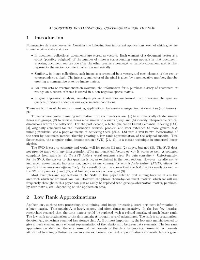
The NMF also has impressive benefits in terms of interpretation of its factors, which is, again, aconsequence of the nonnegativity constraints. For example, consider a text processing application thatrequires the factorization of a term-by-document matrix Am×n. In this case, k can be considered thenumber of (hidden) topics present in the document collection. In this case, Wm×k becomes a term-by-topic matrix whose columns are the NMF basis vectors. The nonzero elements of column 1 of W(denoted W1), which is sparse and nonnegative, correspond to particular terms. By considering the highestweighted terms in this vector, one can assign a label or topic to basis vector 1. Figure 1 shows four basisvectors for one particular term-by-document matrix, the medlars dataset of medical abstracts, available athttp://www.cs.utk.edu/~lsi/. For those familiar with the domain of this dataset, the NMF allows usersthe ability to interpret the basis vectors. For instance, a user might attach the label “heart” to basis vectorW1 of Figure 1. Similar interpretation holds for the other factor H. Hk×n becomes a topic-by-documentmatrix with sparse nonnegative columns. Element j of column 1 of H measures the strength to which topicj appears in document 1.

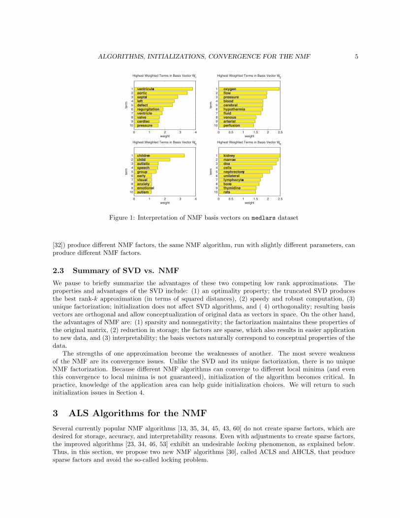
Another fascinating application of the NMF is image processing. Figure 2 clearly demonstrates twoadvantages of the NMF over the SVD. First, notice that the NMF basis vectors, represented as individualblocks in the W matrix, are very sparse (i.e., there is much white space). Similarly, the weights, representedas individual blocks in the Hi vector, are also sparse. On the other hand, the SVD factors are nearlycompletely dense. Second, the basis vectors of the NMF, in the W matrix, have a nice interpretation, asindividual components of the structure of the face—ears, noses, mouths, hairlines. The SVD basis vectorsdo not create an additive parts-based representation. In addition, the gains in storage and interpretabilitydo not come at a loss in performance. The NMF and the SVD perform equally well in reconstructing anapproximation to the original image.

Of course, the NMF has its disadvantages too. Other popular factorizations, especially the SVD, havestrengths concerning uniqueness and robust computation. Yet these become problems for the NMF. Thereis no unique global minimum for the NMF. The optimization problem of Equation (2) is convex in eitherW or H, but not in both W and H, which means that the algorithms can only, if at all, guaranteeconvergence to a local minimum. In practice, NMF users often compare the local minima from severaldifferent starting points, using the results of the best local minimum found. However, this is prohibitiveon large, realistically-sized problems. Not only will different NMF algorithms (and there are many now


0 1 2 3 4

10

9

8

7

6

5

4

3

2

1 ventricularaorticseptalleftdefectregurgitationventriclevalvecardiacpressure

Highest Weighted Terms in Basis Vector W*1

weight

term

0 0.5 1 1.5 2 2.5

10

9

8

7

6

5

4

3

2

1 oxygenflowpressurebloodcerebralhypothermiafluidvenousarterialperfusion


weight

term

0 1 2 3 4

10

9

8

7

6

5

4

3

2

1 childrenchildautisticspeechgroupearlyvisualanxietyemotionalautism


weight

term

0 0.5 1 1.5 2 2.5

10

9

8

7

6

5

4

3

2

1 kidneymarrowdnacellsnephrectomyunilaterallymphocytesbonethymidinerats


weight

term

Figure 1: Interpretation of NMF basis vectors on medlars dataset

[32]) produce different NMF factors, the same NMF algorithm, run with slightly different parameters, canproduce different NMF factors.

2.3 Summary of SVD vs. NMF

We pause to briefly summarize the advantages of these two competing low rank approximations. Theproperties and advantages of the SVD include: (1) an optimality property; the truncated SVD producesthe best rank-k approximation (in terms of squared distances), (2) speedy and robust computation, (3)unique factorization; initialization does not affect SVD algorithms, and ( 4) orthogonality; resulting basisvectors are orthogonal and allow conceptualization of original data as vectors in space. On the other hand,the advantages of NMF are: (1) sparsity and nonnegativity; the factorization maintains these properties ofthe original matrix, (2) reduction in storage; the factors are sparse, which also results in easier applicationto new data, and (3) interpretability; the basis vectors naturally correspond to conceptual properties of thedata.

The strengths of one approximation become the weaknesses of another. The most severe weaknessof the NMF are its convergence issues. Unlike the SVD and its unique factorization, there is no uniqueNMF factorization. Because different NMF algorithms can converge to different local minima (and eventhis convergence to local minima is not guaranteed), initialization of the algorithm becomes critical. Inpractice, knowledge of the application area can help guide initialization choices. We will return to suchinitialization issues in Section 4.

3 ALS Algorithms for the NMF

Several currently popular NMF algorithms [13, 35, 34, 45, 43, 60] do not create sparse factors, which aredesired for storage, accuracy, and interpretability reasons. Even with adjustments to create sparse factors,the improved algorithms [23, 34, 46, 53] exhibit an undesirable locking phenomenon, as explained below.Thus, in this section, we propose two new NMF algorithms [30], called ACLS and AHCLS, that producesparse factors and avoid the so-called locking problem.


SVD

W H

A i

i

U ViΣ

Figure 2: Interpretation of NMF and SVD basis vectors on face dataset, from [35]

Both algorithms are modifications to the simple Alternating Least Squares (ALS) algorithm [45], whereinW is fixed and H is computed using least squares, then H is fixed and W is computed using leastsquares, and so on, in alternating fashion. The method of alternating variables is a well-known techniquein optimization [42]. One problem with the first ALS algorithm applied to the NMF problem (done byPaatero and Tapper in 1994 [45]) was the lack of sparsity restrictions. To address this, the ACLS algorithmadds a reward for sparse factors of the NMF. The user sets the two parameters λH and λW to positivevalues. Increasing these values increases the sparsity of the two NMF factors. However, because there areno upperbounds on these parameters, a user must resort to trial and error to find the best values for λHand λW . The more advanced AHCLS [30], presented in Section 3.2, provides better sparsity parameterswith more intuitive bounds.

3.1 The ACLS Algorithm

The ACLS (Alternating Constrained Least Squares) algorithm is implemented differently than the originalALS algorithm [45] because issues arise at each alternating step, where a constrained least squares problemof the following form

minhj

‖aj −Whj‖22 + λH‖hj‖22 s.t. λH ≥ 0,hj ≥ 0 (2)

must be solved. The vectors aj and hj are columns of A and H, respectively. Notice that the decisionvariable hj must be nonnegative. There are algorithms specifically designed for this nonnegative constrained


least squares problem. In fact, the NNLS algorithm of Lawson and Hanson [8, 33] is so common that itappears as a built-in function in MATLAB. Unfortunately, the NNLS algorithm is very slow, as it is an“active set” method, meaning it can swap only one variable from the basis at a time. Even the fasterversion of the NNLS algorithm by Bro and de Jong [11] is still not fast enough, and the NNLS step remainsthe computational bottleneck. As a result, in practice, compromises are made. For example, a standard(unconstrained) least squares step is run [8] and all negative elements in the solution vector are set to 0.This ad-hoc enforcement of nonnegativity, while not theoretically appealing, works quite well in practice.The practical ACLS algorithm is shown below.

Practical ACLS Algorithm for NMF

input λW , λHW = rand(m,k); % initialize W as random dense matrix or use another initialization from Section 4

for i = 1 : maxiter(cls) Solve for H in matrix equation (WTW + λHI) H = WTA. % for W fixed, find H

(nonneg) Set all negative elements in H to 0.(cls) Solve for W in matrix equation (HHT + λW I) WT = HAT . % for H fixed, find W

(nonneg) Set all negative elements in W to 0.end

3.2 The AHCLS Algorithm

ACLS uses a crude measure ‖x‖22 to approximate the sparsity of a vector x. The AHCLS replaces this witha more sophisticated measure, spar(x), which was invented by Hoyer [24].

spar(xn×1) =

√n− ‖x‖1/‖x‖2√n− 1

In AHCLS (Alternating Hoyer-Constrained Least Squares), the user defines two scalars αW and αH inaddition to λH and λW of ACLS. For AHCLS, the two additional scalars 0 ≤ αW , αH ≤ 1 represent auser’s desired sparsity in each column of the factors. These scalars, because they range from 0 to 1, matchnicely with a user’s notion of sparsity as a percentage. Recall that 0 ≤ λW , λH ≤ ∞ are positive weightsassociated with the penalties assigned to the density of W and H. Thus, in AHCLS, they measure howimportant it is to the user that spar(Wj∗) = αW and spar(Hj∗) = αH . Our experiments show thatAHCLS does a better job of enforcing sparsity than ACLS does. And the four AHCLS parameters areeasier to set. For example, as a guideline, we recommend 0 ≤ λW , λH ≤ 1, with of course, 0 ≤ αW , αH ≤ 1.The practical AHCLS algorithm, using matrix systems and ad-hoc enforcement of negativity, is below. Eis the matrix of all ones.

Practical AHCLS Algorithm for NMF

input λW , λH , αW , αH W = rand(m,k); % initialize W as random dense matrix or use another initialization

from Section 4

βH = ((1− αH)√k + αH)2

βW = ((1− αW )√k + αW )2

for i = 1 : maxiter(hcls) Solve for H in matrix equation (WTW + λHβHI− λHE) H = WTA.(nonneg) Set all negative elements in H to 0.(hcls) Solve for W in matrix equation (HHT + λWβW I− λWE) WT = HAT .(nonneg) Set all negative elements in W to 0.

end


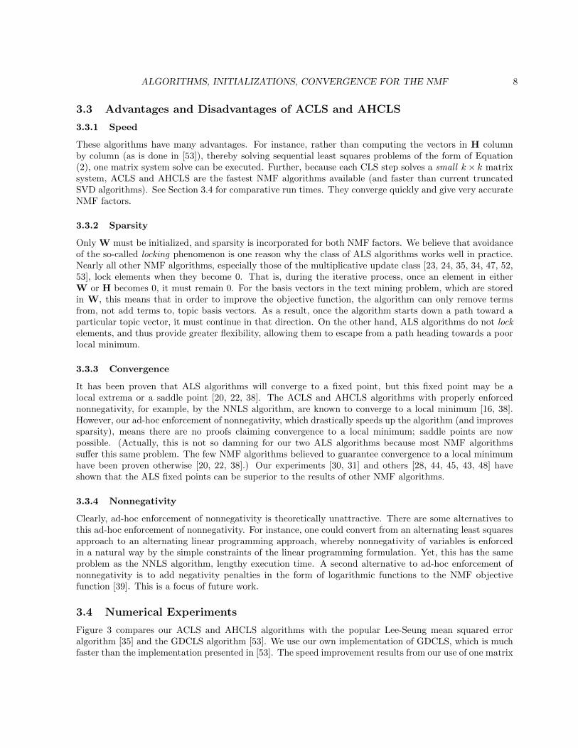
3.3 Advantages and Disadvantages of ACLS and AHCLS

3.3.1 Speed

These algorithms have many advantages. For instance, rather than computing the vectors in H columnby column (as is done in [53]), thereby solving sequential least squares problems of the form of Equation(2), one matrix system solve can be executed. Further, because each CLS step solves a small k× k matrixsystem, ACLS and AHCLS are the fastest NMF algorithms available (and faster than current truncatedSVD algorithms). See Section 3.4 for comparative run times. They converge quickly and give very accurateNMF factors.

3.3.2 Sparsity

Only W must be initialized, and sparsity is incorporated for both NMF factors. We believe that avoidanceof the so-called locking phenomenon is one reason why the class of ALS algorithms works well in practice.Nearly all other NMF algorithms, especially those of the multiplicative update class [23, 24, 35, 34, 47, 52,53], lock elements when they become 0. That is, during the iterative process, once an element in eitherW or H becomes 0, it must remain 0. For the basis vectors in the text mining problem, which are storedin W, this means that in order to improve the objective function, the algorithm can only remove termsfrom, not add terms to, topic basis vectors. As a result, once the algorithm starts down a path toward aparticular topic vector, it must continue in that direction. On the other hand, ALS algorithms do not lockelements, and thus provide greater flexibility, allowing them to escape from a path heading towards a poorlocal minimum.

3.3.3 Convergence

It has been proven that ALS algorithms will converge to a fixed point, but this fixed point may be alocal extrema or a saddle point [20, 22, 38]. The ACLS and AHCLS algorithms with properly enforcednonnegativity, for example, by the NNLS algorithm, are known to converge to a local minimum [16, 38].However, our ad-hoc enforcement of nonnegativity, which drastically speeds up the algorithm (and improvessparsity), means there are no proofs claiming convergence to a local minimum; saddle points are nowpossible. (Actually, this is not so damning for our two ALS algorithms because most NMF algorithmssuffer this same problem. The few NMF algorithms believed to guarantee convergence to a local minimumhave been proven otherwise [20, 22, 38].) Our experiments [30, 31] and others [28, 44, 45, 43, 48] haveshown that the ALS fixed points can be superior to the results of other NMF algorithms.

3.3.4 Nonnegativity

Clearly, ad-hoc enforcement of nonnegativity is theoretically unattractive. There are some alternatives tothis ad-hoc enforcement of nonnegativity. For instance, one could convert from an alternating least squaresapproach to an alternating linear programming approach, whereby nonnegativity of variables is enforcedin a natural way by the simple constraints of the linear programming formulation. Yet, this has the sameproblem as the NNLS algorithm, lengthy execution time. A second alternative to ad-hoc enforcement ofnonnegativity is to add negativity penalties in the form of logarithmic functions to the NMF objectivefunction [39]. This is a focus of future work.

3.4 Numerical Experiments

Figure 3 compares our ACLS and AHCLS algorithms with the popular Lee-Seung mean squared erroralgorithm [35] and the GDCLS algorithm [53]. We use our own implementation of GDCLS, which is muchfaster than the implementation presented in [53]. The speed improvement results from our use of one matrix


system rather than serial vector systems to solve the CLS step. This implementation trick was describedabove for the ACLS and AHCLS algorithms.

To create Figure 3, we used the medlars dataset of medical abstracts and the cisi dataset of libraryscience abstracts. These figures clearly show how the ALS-type algorithms outperform the Lee-Seungmultiplicative update algorithms in terms of accuracy and speed. While the ALS-type algorithms providesimilar accuracy to the GDCLS algorithm, they are much faster. This speed advantage continues to hold formuch larger collections like the reuters10 collection, used in Section 4. (Details on the reuters10 datasetappear in Section 4.3.) On average the ACLS and AHCLS algorithms require roughly 2/3 the time of theGDCLS algorithm. Figure 3 also reports the error in the optimal rank-10 approximation required by theSVD. Notice how close all NMF algorithms come to the optimal factorization error. Also, notice that ACLSand AHCLS require less time than the SVD to produce such good, sparse, nonnegative factorizations.

0 5 10 15 20 25 30118.5

119

119.5

120

120.5

121

121.5

122

122.5

123

123.5

iteration

||A

W

H|| 2

SVD error = 118.49

Lee Seung (30.2 sec)

GDCLS (1.49 sec)

ACLS (.92 sec)

AHCLS (.90 sec)

SVD time = 1.42 sec

0 5 10 15 20 25 30116

116.5

117

117.5

118

118.5

119

119.5

120

120.5

iteration

||A

W

H|| 2

SVD error = 116.16

Lee Seung (57.8 sec)

GDCLS (1.76 sec)

ACLS (1.06 sec)

AHCLS (1.04 sec)

SVD time = 1.09 sec

Figure 3: Accuracy and Run-times of NMF Algorithms on medlars (left) and cisi (right) datasets

4 Initializations

All NMF algorithms are iterative and it is well-known that they are sensitive to the initialization of Wand H [56]. Some algorithms require that both W and H be initialized [23, 24, 35, 34, 46], while othersrequire initialization of only W [45, 43, 52, 53]. In all cases, a good initialization can improve the speedand accuracy of the algorithms, as it can produce faster convergence to an improved local minimum [55].A good initialization can sidestep some of the convergence problems mentioned above, which is preciselywhy they are so important. In this section, we compare several initialization procedures (two old and fournew) by testing them on the ALS algorithms presented in Section 3. We choose to use the ACLS andAHCLS algorithms because they produce sparse accurate factors and require about the same time as theSVD. Most other NMF algorithms require much more time than the SVD, often times orders of magnitudemore time.

4.1 Two Existing Initializations

Nearly all NMF algorithms use simple random initialization, i.e., W and H are initialized as dense matricesof random numbers between 0 and 1. It is well-known that random initialization does not generally providea good first estimate for NMF algorithms [55], especially those of the ALS-type of [12, 37, 49, 51]. Wildet al. [56, 57, 58] have shown that the centroid initialization, built from the centroid decomposition [15]


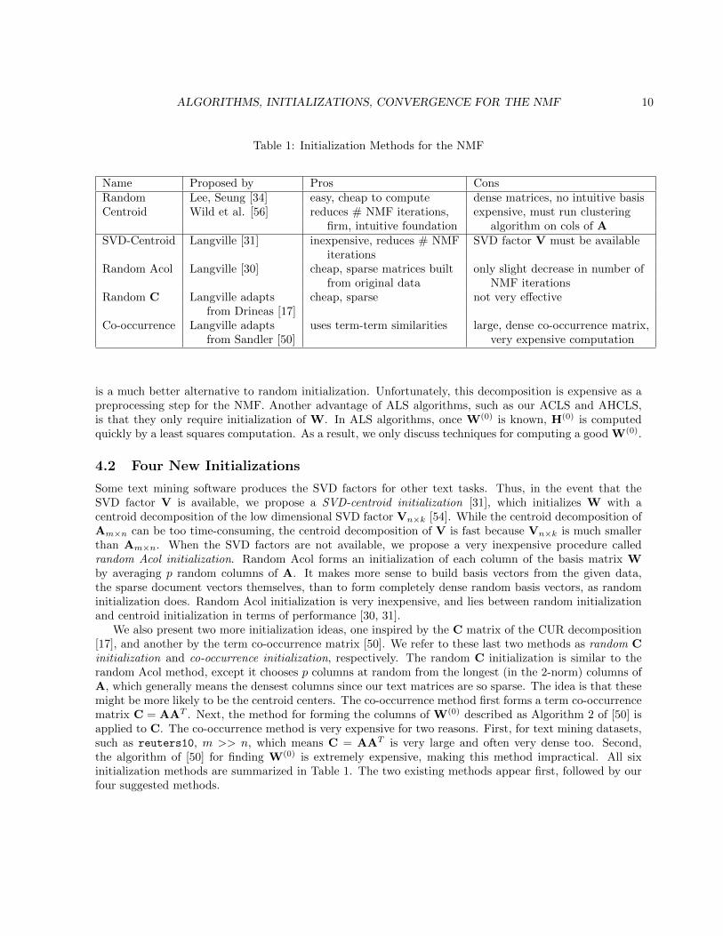
Table 1: Initialization Methods for the NMF

Name Proposed by Pros ConsRandom Lee, Seung [34] easy, cheap to compute dense matrices, no intuitive basisCentroid Wild et al. [56] reduces # NMF iterations, expensive, must run clustering

firm, intuitive foundation algorithm on cols of ASVD-Centroid Langville [31] inexpensive, reduces # NMF SVD factor V must be available

iterationsRandom Acol Langville [30] cheap, sparse matrices built only slight decrease in number of

from original data NMF iterationsRandom C Langville adapts cheap, sparse not very effective

from Drineas [17]Co-occurrence Langville adapts uses term-term similarities large, dense co-occurrence matrix,

from Sandler [50] very expensive computation

is a much better alternative to random initialization. Unfortunately, this decomposition is expensive as apreprocessing step for the NMF. Another advantage of ALS algorithms, such as our ACLS and AHCLS,is that they only require initialization of W. In ALS algorithms, once W(0) is known, H(0) is computedquickly by a least squares computation. As a result, we only discuss techniques for computing a good W(0).

4.2 Four New Initializations

Some text mining software produces the SVD factors for other text tasks. Thus, in the event that theSVD factor V is available, we propose a SVD-centroid initialization [31], which initializes W with acentroid decomposition of the low dimensional SVD factor Vn×k [54]. While the centroid decomposition ofAm×n can be too time-consuming, the centroid decomposition of V is fast because Vn×k is much smallerthan Am×n. When the SVD factors are not available, we propose a very inexpensive procedure calledrandom Acol initialization. Random Acol forms an initialization of each column of the basis matrix Wby averaging p random columns of A. It makes more sense to build basis vectors from the given data,the sparse document vectors themselves, than to form completely dense random basis vectors, as randominitialization does. Random Acol initialization is very inexpensive, and lies between random initializationand centroid initialization in terms of performance [30, 31].

We also present two more initialization ideas, one inspired by the C matrix of the CUR decomposition[17], and another by the term co-occurrence matrix [50]. We refer to these last two methods as random Cinitialization and co-occurrence initialization, respectively. The random C initialization is similar to therandom Acol method, except it chooses p columns at random from the longest (in the 2-norm) columns ofA, which generally means the densest columns since our text matrices are so sparse. The idea is that thesemight be more likely to be the centroid centers. The co-occurrence method first forms a term co-occurrencematrix C = AAT . Next, the method for forming the columns of W(0) described as Algorithm 2 of [50] isapplied to C. The co-occurrence method is very expensive for two reasons. First, for text mining datasets,such as reuters10, m >> n, which means C = AAT is very large and often very dense too. Second,the algorithm of [50] for finding W(0) is extremely expensive, making this method impractical. All sixinitialization methods are summarized in Table 1. The two existing methods appear first, followed by ourfour suggested methods.


Table 2: Experiments with Initialization Methods for the NMF

Method Time W(0) Storage W(0) Error(0) Error(10) Error(20) Error(30)Random .09 sec 726K 4.28% .28% .15% .15%Centroid 27.72 46K 2.02% .27% .18% .18%SVD-Centroid .65† 56K 2.08% .06% .06% .06%Random Acol∗ .05 6K 2.01% .21% .16% .15%Random C◦ .11 22K 3.35% .29% .20% .19%Co-occurrence 3287 45K 3.38% .37% .27% .25%ACLS time .37 sec 3.42 6.78 10.29

† provided V of the SVD is already available∗ each column of W(0) formed by averaging 20 random columns of A◦ each column of W(0) formed by averaging 20 of the longest columns of A

4.3 Initialization Experiments with Reuters10 dataset

The reuters10 collection is our subset of the Reuters-21578 version of the Reuter’s benchmark documentcollection of business newswire posts. The Reuters-21578 version contains over 20,000 documents catego-rized into 118 different categories, and is available online.1 Our subset, the reuters10 collection, is derivedfrom the set of documents that have been classified into the top ten most frequently occurring categories.The collection contains 9248 documents from the training data of the “ModApte split” (details of the splitare also available at the website above).

The numbers reported in Table 2 were generated by applying the alternating constrained least squares(ACLS) algorithm of Section 3 with λH = λW = .5 to the reuters10 dataset. The error measure in thistable is relative to the optimal rank-10 approximation given by the singular value decomposition. For thisdataset, ‖A−U10Σ10V

T10‖F = 22656. Thus, for example, the error at iteration 10 is computed as

Error(10) =‖A−W(10)H(10)‖F − 22656

22656.

We distinguish between quantitative accuracy, as reported in Table 2, and qualitative accuracy asreported in Tables 3 through 9. For text mining applications, it is often not essential that the low rankapproximation be terribly precise. Often suboptimal solutions are “good enough.” After reviewing Tables3–9, it is easy to see why some initializations give better accuracy and converge more quickly. They startwith basis vectors in W(0) that are much closer to the best basis vectors found, as reported in Table 3,which was generated by using the basis vectors associated with the best global minimum for the reuters10dataset, found by using 500 random restarts. In fact, the relative error for this global minimum is .009%,showing remarkable closeness to the optimal rank-10 approximation. By comparing each subsequent tablewith Table 3, it’s clear why one initialization method is better than another. The best method, SVD-centroid initialization, starts with basis vectors very close to the “optimal” basis vectors of Table 3. Onthe other hand, random and random Acol initialization are truly random. Nevertheless, random Acol doesmaintain one clear advantage over random initialization as it creates a very sparse W(0). The RandomC and co-occurrence initializations suffer from lack of diversity. Many of the longest documents in thereuters10 collection appear to be on similar topics, thus, not allowing W(0) to cover many of the reuterstopics.

Because the algorithms did not produce the “wheat” vector always in column one of W, we havereordered the resulting basis vectors in order to make comparisons easier. We also note that the nonnegative

1http://www.daviddlewis.com/resources/testcollections/reuters21578/


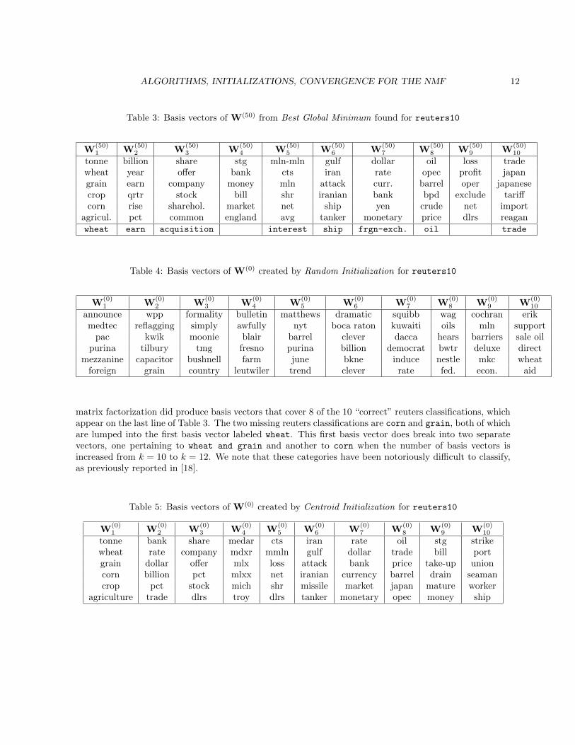
Table 3: Basis vectors of W(50) from Best Global Minimum found for reuters10

W(50)1 W

(50)2 W

(50)3 W

(50)4 W

(50)5 W

(50)6 W

(50)7 W

(50)8 W

(50)9 W

(50)10

tonne billion share stg mln-mln gulf dollar oil loss tradewheat year offer bank cts iran rate opec profit japangrain earn company money mln attack curr. barrel oper japanesecrop qrtr stock bill shr iranian bank bpd exclude tariffcorn rise sharehol. market net ship yen crude net import

agricul. pct common england avg tanker monetary price dlrs reaganwheat earn acquisition interest ship frgn-exch. oil trade

Table 4: Basis vectors of W(0) created by Random Initialization for reuters10

W(0)1 W

(0)2 W

(0)3 W

(0)4 W

(0)5 W

(0)6 W

(0)7 W

(0)8 W

(0)9 W

(0)10

announce wpp formality bulletin matthews dramatic squibb wag cochran erikmedtec reflagging simply awfully nyt boca raton kuwaiti oils mln support

pac kwik moonie blair barrel clever dacca hears barriers sale oilpurina tilbury tmg fresno purina billion democrat bwtr deluxe direct

mezzanine capacitor bushnell farm june bkne induce nestle mkc wheatforeign grain country leutwiler trend clever rate fed. econ. aid

matrix factorization did produce basis vectors that cover 8 of the 10 “correct” reuters classifications, whichappear on the last line of Table 3. The two missing reuters classifications are corn and grain, both of whichare lumped into the first basis vector labeled wheat. This first basis vector does break into two separatevectors, one pertaining to wheat and grain and another to corn when the number of basis vectors isincreased from k = 10 to k = 12. We note that these categories have been notoriously difficult to classify,as previously reported in [18].

Table 5: Basis vectors of W(0) created by Centroid Initialization for reuters10

W(0)1 W

(0)2 W

(0)3 W

(0)4 W

(0)5 W

(0)6 W

(0)7 W

(0)8 W

(0)9 W

(0)10

tonne bank share medar cts iran rate oil stg strikewheat rate company mdxr mmln gulf dollar trade bill portgrain dollar offer mlx loss attack bank price take-up unioncorn billion pct mlxx net iranian currency barrel drain seamancrop pct stock mich shr missile market japan mature worker

agriculture trade dlrs troy dlrs tanker monetary opec money ship


Table 6: Basis vectors of W(0) created by SVD-Centroid Initialization for reuters10

W(0)1 W

(0)2 W

(0)3 W

(0)4 W

(0)5 W

(0)6 W

(0)7 W

(0)8 W

(0)9 W

(0)10

tonne billion share bank cts iran dollar oil loss tradewheat year offer money shr gulf rate barrel oper japangrain earn company rate mln attack curr. opec profit japanesecorn qrtr stock stg net iranian yen crude cts tariffcrop rise pct market mln-mln missile japan bpd mln import

agricul. pct common pct rev ship economic price net country

Table 7: Basis vectors of W(0) created by Random Acol Initialization for reuters10

W(0)1 W

(0)2 W

(0)3 W

(0)4 W

(0)5 W

(0)6 W

(0)7 W

(0)8 W

(0)9 W

(0)10

mln fee agl mln mark loss official dlrs bank tradedenman mortg. tmoc dlrs mannes. mln piedmont oper bancaire viermetz

dlrs billion bank share dividend cts dollar billion austral mlnecuador winley pct seipp mln maki interest loss neworld nwa

venezuela mln company billion dieter name tokyo texaco datron ctsrevenue fed maki dome gpu kato japanese pennzoil share builder

Table 8: Basis vectors of W(0) created by Random C Initialization for reuters10

W(0)1 W

(0)2 W

(0)3 W

(0)4 W

(0)5 W

(0)6 W

(0)7 W

(0)8 W

(0)9 W

(0)10

analyst dollar econ. bank market analyst analyst analyst trade ratelawson rate policy rate bank market industry bank dollar trademarket econ. pct market analyst trade price currency japan officialtrade mark cost currency price pct market japan price bank

sterling bank growth dollar mark last believe billion japanese marketdollar rise trade trade good official last cut pct econ.

Table 9: Basis vectors of W(0) created by Co-occurrence Initialization for reuters10

W(0)1 W

(0)2 W

(0)3 W

(0)4 W

(0)5 W

(0)6 W

(0)7 W

(0)8 W

(0)9 W

(0)10

dept. average agricul. national farmer rate-x aver price plywood wash. tradewheat pct wheat bank rate-x natl average aqtn trade japan

agricul. rate tonne rate natl avge price aequitron japan billiontonne price grain pct avge farmer yield medical official marketusda billion farm oil cwt cwt billion enzon reagan japanesecorn oil dept. gov. wheat wheat bill enzon pct import


5 Convergence Criterion

Nearly all NMF algorithms use the simplest possible convergence criterion, i.e., run for a fixed numberof iterations, denoted maxiter. This criterion is used so often because the natural criterion, stop when‖A−WH‖ ≤ ε, requires more expense than most users are willing to expend, even occasionally. Notice thatmaxiter was the convergence criterion used in the ACLS and AHCLS algorithms of Section 3. However,a fixed number of iterations is not a mathematically appealing way to control the number of iterationsexecuted because the most appropriate value for maxiter is problem-dependent.

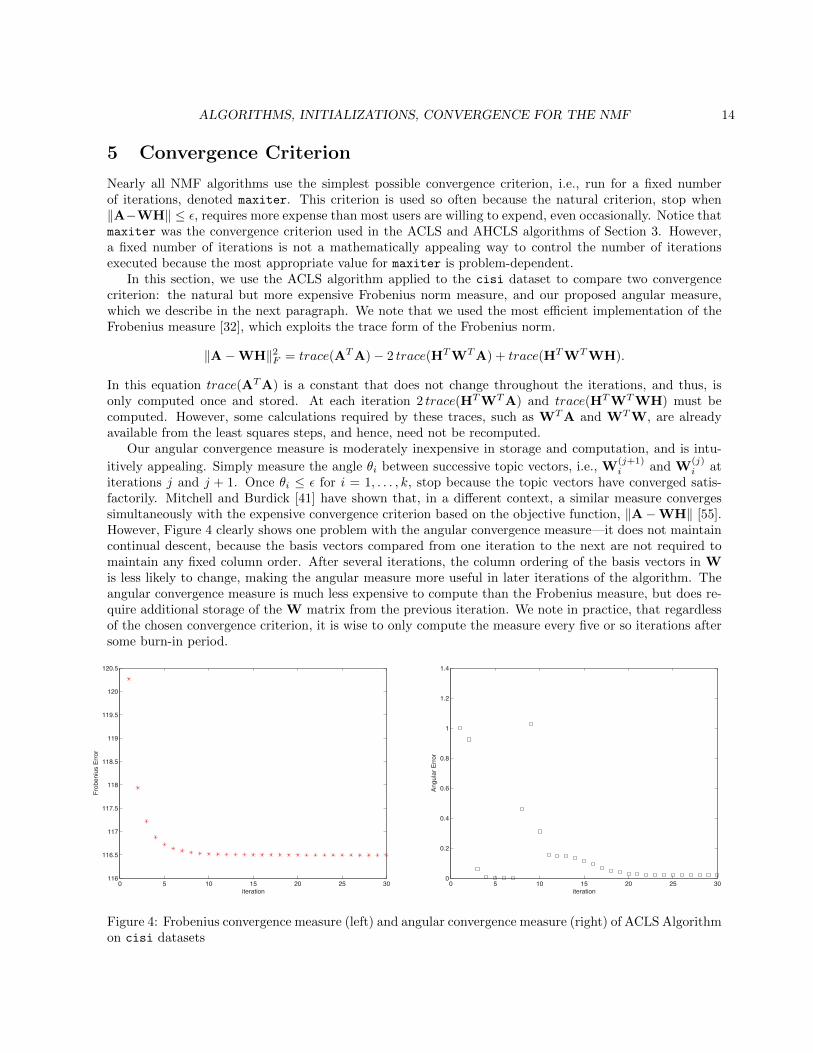
In this section, we use the ACLS algorithm applied to the cisi dataset to compare two convergencecriterion: the natural but more expensive Frobenius norm measure, and our proposed angular measure,which we describe in the next paragraph. We note that we used the most efficient implementation of theFrobenius measure [32], which exploits the trace form of the Frobenius norm.

‖A−WH‖2F = trace(ATA)− 2 trace(HTWTA) + trace(HTWTWH).

In this equation trace(ATA) is a constant that does not change throughout the iterations, and thus, isonly computed once and stored. At each iteration 2 trace(HTWTA) and trace(HTWTWH) must becomputed. However, some calculations required by these traces, such as WTA and WTW, are alreadyavailable from the least squares steps, and hence, need not be recomputed.

Our angular convergence measure is moderately inexpensive in storage and computation, and is intu-

itively appealing. Simply measure the angle θi between successive topic vectors, i.e., W(j+1)i and W

(j)i at

iterations j and j + 1. Once θi ≤ ε for i = 1, . . . , k, stop because the topic vectors have converged satis-factorily. Mitchell and Burdick [41] have shown that, in a different context, a similar measure convergessimultaneously with the expensive convergence criterion based on the objective function, ‖A−WH‖ [55].However, Figure 4 clearly shows one problem with the angular convergence measure—it does not maintaincontinual descent, because the basis vectors compared from one iteration to the next are not required tomaintain any fixed column order. After several iterations, the column ordering of the basis vectors in Wis less likely to change, making the angular measure more useful in later iterations of the algorithm. Theangular convergence measure is much less expensive to compute than the Frobenius measure, but does re-quire additional storage of the W matrix from the previous iteration. We note in practice, that regardlessof the chosen convergence criterion, it is wise to only compute the measure every five or so iterations aftersome burn-in period.

0 5 10 15 20 25 30116

116.5

117

117.5

118

118.5

119

119.5

120

120.5

iteration

Fro

be

niu

s E

rro

r

0 5 10 15 20 25 300

0.2

0.4

0.6

0.8

1

1.2

1.4

iteration

An

gu

lar

Err

or

Figure 4: Frobenius convergence measure (left) and angular convergence measure (right) of ACLS Algorithmon cisi datasets


The recent 2005 reference by Lin [38] mentioned the related convergence criterion issue of stationarity.The fact that ‖A −WH‖ (or some similar objective function) levels off does not guarantee stationarity.Lin advocates a stationarity check once an algorithm has stopped. For instance, the stationarity checksof Chu and Plemmons [13] may be used. Lin [38] proposes a convergence criterion, that simultaneouslychecks for stationarity, and fits nicely into his projected gradients algorithm. We agree that a stationaritycheck should be conducted on termination.

6 Conclusion

The two new NMF algorithms presented in this paper, ACLS and AHCLS, are some of the fastest available,even faster than truncated SVD algorithms. However, while the algorithms will converge to a stationarypoint, they cannot guarantee that this stationary point is a local minimum. If a local minimum must beachieved, then we recommend using the results from a fast ALS-type algorithm as the initialization forone of the slow algorithms [38] that do guarantee convergence to a local minimum. In this paper we alsopresented several alternatives to the common, but poor, initialization technique of random initialization.Lastly, we proposed an alternative stopping criterion that practical implementations of NMF code shouldconsider. The common stopping criterion of running for a fixed number of iterations should be replacedwith a criterion that fits the context of the users and their data. For many applications, iterating until‖A−WH‖ reaches some small level is unnecessary, especially in cases where one is most interested in thequalitative results produced by the vectors in W. In such cases, our proposed angular convergence measureis more appropriate.

References

[1] Ricardo Baeza-Yates and Berthier Ribeiro-Neto. Modern Information Retrieval. ACM Press, NewYork, 1999.

[2] R. Barrett, M. Berry, T. F. Chan, J. Demmel, J. Donato, J. Dongarra, V. Eijkhout, R. Pozo, C. Romine,and H. Van der Vorst. Templates for the Solution of Linear Systems: Building Blocks for IterativeMethods. SIAM, Philadelphia, 2nd edition, 1994.

[3] Michael W. Berry, editor. Computational Information Retrieval. SIAM, Philadelphia, 2001.

[4] Michael W. Berry and Murray Browne. Understanding Search Engines: Mathematical Modeling andText Retrieval. SIAM, Philadelphia, 2nd edition, 2005.

[5] Michael W. Berry, Zlatko Drmac, and Elizabeth R. Jessup. Matrices, vector spaces and informationretrieval. SIAM Review, 41:335–62, 1999.

[6] Michael W. Berry and R. D. Fierro. Low-rank orthogonal decompositions for information retrievalapplications. Journal of Numerical Linear Algebra with Applications, 1(1):1–27, 1996.

[7] Michael W. Berry and Gavin W. O’Brien. Using linear algebra for intelligent information retrieval.SIAM Review, 37:573–595, 1998.

[8] Ake Bjorck. Numerical methods for least squares problems. SIAM, Philadelphia, 1996.

[9] Katarina Blom. Information retrieval using the singular value decomposition and Krylov subspaces.PhD thesis, University of Chalmers, January 1999.

[10] Katarina Blom and Axel Ruhe. Information retrieval using very short Krylov sequences. In Compu-tational Information Retrieval, pages 41–56, 2001.


[11] Rasmus Bro and Sijmen de Jong. A fast non-negativity constrained linear least squares algorithm.Journal of Chemometrics, 11:393–401, 1997.

[12] Donald S. Burdick, Xin M. Tu, Linda B. McGown, and David W. Millican. Resolution of multi-component fluorescent mixtures by analysis of the excitation-emission-frequency array. Journal ofChemometrics, 4:15–28, 1990.

[13] Moody Chu, Fasma Diele, Robert J. Plemmons, and Stefania Ragni. Optimality, computation, andinterpretations of nonnegative matrix factorizations. SIAM Journal on Matrix Analysis, 2004. sub-mitted.

[14] Anirban Dasgupta, Ravi Kumar, Prabhakar Raghavan, and Andrew Tomkins. Variable latent semanticindexing. In Proceeding of the eleventh ACM SIGKDD international conference on Knowledge discoveryin data mining. ACM Press, 2005.

[15] Inderjit S. Dhillon. Concept decompositions for large sparse text data using clustering. MachineLearning, 42(1/2):143–175, 2001.

[16] Inderjit S. Dhillon and Suvrit Sra. Generalized nonnegative matrix approximations with Bregman di-vergences. In Proceeding of the Neural Information Processing Systems (NIPS) Conference, Vancouver,B.C., 2005.

[17] Petros Drineas, Ravi Kannan, and Michael W. Mahoney. Fast Monte Carlo algorithms for matricesIII: Computing a compressed approximate matrix decomposition. SIAM Journal on Computing, 2006.to appear.

[18] Susan Dumais, John Platt, David Heckerman, and Mehran Sahami. Inductive learning algorithmsand representations for text categorization. In CIKM ’98: Proceedings of the seventh internationalconference on Information and knowledge management, pages 148–55. ACM Press, 1998.

[19] Susan T. Dumais. Improving the retrieval of information from external sources. Behavior ResearchMethods, Instruments and Computers, 23:229–236, 1991.

[20] Lorenzo Finesso and Peter Spreij. Approximate nonnegative matrix factorization via alternating min-imization. In Sixteenth International Symposium on Mathematical Theory of Networks and Systems,Leuven, 2004.

[21] Gene H. Golub and Charles F. Van Loan. Matrix Computations. Johns Hopkins University Press,Baltimore, 1996.

[22] Edward F. Gonzalez and Yin Zhang. Accelerating the Lee-Seung algorithm for nonnegative matrixfactorization. Technical Report TR-05-02, Rice University, March 2005.

[23] Patrik O. Hoyer. Non-negative sparse coding. In Neural Networks for Signal Processing XII (Proc.IEEE Workshop on Neural Networks for Signal Processing), pages 557–565, 2002.

[24] Patrik O. Hoyer. Non-negative matrix factorization with sparseness constraints. Journal of MachineLearning Research, 5:1457–1469, 2004.

[25] M. K. Hughey and Michael W. Berry. Improved query matching using kd-trees, a latent semanticindexing enhancement. Information Retrieval, 2:287–302, 2000.

[26] Eric P. Jiang and Michael W. Berry. Solving total least squares problems in information retrieval.Linear Algebra and its Applications, 316:137–156, 2000.


[27] Fan Jiang and Michael L. Littman. Approximate dimension equalization in vector-based informationretrieval. In The Seventeenth International Conference on Machine Learning, pages 423–430, 2000.

[28] Mika Juvela, Kimmi Lehtinen, and Pentti Paatero. The use of positive matrix factorization in theanalysis of molecular line spectra. Monthly Notices of the Royal Astronomical Society, 280:616–626,1996.

[29] Tamara G. Kolda and Dianne P. O’Leary. A semi-discrete matrix decomposition for latent semanticindexing in information retrieval. ACM Transactions on Information Systems, 16:322–346, 1998.

[30] Amy N. Langville. Algorithms for the nonnegative matrix factorization in text mining, April 2005.Slides from SAS Meeting.

[31] Amy N. Langville. Experiments with the nonnegative matrix factorization and the reuters10 dataset,February 2005. Slides from SAS Meeting.

[32] Amy N. Langville, Michael W. Berry, Murray Browne, V. Paul Pauca, and Robert J. Plemmons. Al-gorithms and applications for approximate nonnegative matrix factorization. Computational Statisticsand Data Analysis, 52(1):155–173, 2007.

[33] Charles L. Lawson and Richard J. Hanson. Solving Least Squares Problems. SIAM, 1995.

[34] D. Lee and H. Seung. Algorithms for Non-Negative Matrix Factorization. Advances in Neural Infor-mation Processing Systems, 13:556–562, 2001.

[35] Daniel D. Lee and H. Sebastian Seung. Learning the parts of objects by non-negative matrix factor-ization. Nature, 401:788–791, 1999.

[36] Todd A. Letsche and Michael W. Berry. Large-scale information retrieval with LSI. Informatics andComputer Science, pages 105–137, 1997.

[37] Shousong Li and Paul J. Gemperline. Eliminating complex eigenvectors and eigenvalues in multiwayanalyses using the direct trilinear decomposition method. Journal of Chemometrics, 7:77–88, 1993.

[38] Chih-Jen Lin. Projected gradient methods for non-negative matrix factorization. Technical ReportInformation and Support Services Tech. Report ISSTECH-95-013, Department of Computer Science,National Taiwan University, 2005.

[39] Jianhang Lu and Laosheng Wu. Technical details and programming guide for a general two-waypositive matrix factorization algorithm. Journal of Chemometrics, 18:519–525, 2004.

[40] Carl D. Meyer. Matrix Analysis and Applied Linear Algebra. SIAM, Philadelphia, 2000.

[41] Ben C. Mitchell and Donald S. Burdick. Slowly converging PARAFAC sequences: Swamps and two-factor degeneracies. Journal of Chemometrics, 8:155–168, 1994.

[42] Jorge Nocedal and Stephen J. Wright. Numerical Optimization. Springer, 1999.

[43] Pentti Paatero. Least squares formulation of robust non-negative factor analysis. Chemometrics andIntelligent Laboratory Systems, 37:23–35, 1997.

[44] Pentti Paatero. The multilinear engine—a table-driven least squares program for solving multilinearproblems, including the n-way parallel factor analysis model. Journal of Computational and GraphicalStatistics, 8(4):1–35, 1999.

[45] Pentti Paatero and U. Tapper. Positive matrix factorization: a non-negative factor model with optimalutilization of error estimates of data values. Environmetrics, 5:111–126, 1994.


[46] V. Paul Pauca, Jon Piper, and Robert J. Plemmons. Nonnegative matrix factorization for spectraldata analysis. 2005.

[47] V. Paul Pauca, Farial Shahnaz, Michael W. Berry, and Robert J. Plemmons. Text Mining UsingNon-Negative Matrix Factorizations. In Proceedings of the Fourth SIAM International Conference onData Mining, April 22-24, Lake Buena Vista, FL, 2004. SIAM.

[48] Robert J. Plemmons, 2005. private communication.

[49] E. Sanchez and B. R. Kowalski. Tensorial resolution: A direct trilinear decomposition. Journal ofChemometrics, 4:29–45, 1990.

[50] Mark Sandler. On the use of linear programming for unsupervised text classification. In The EleventhACM SIGKDD International Conference on Knowledge Discovery and Data Mining, Chicago, IL,2005.

[51] R. Sands and Forrest W. Young. Component models for three-way data: an alternating least squaresalgorithm with optimal scaling features. Psychometrika, 45:39–67, 1980.

[52] Farial Shahnaz. A clustering method based on nonnegative matrix factorization for text mining.Master’s thesis, University of Tennessee, Knoxville, 2004.

[53] Farial Shahnaz, Michael W. Berry, V.Paul Pauca, and Robert J. Plemmons. Document ClusteringUsing Nonnegative Matrix Factorization. Information Processing & Management, 42(2):373–386, 2006.

[54] David B. Skillicorn, S. M. McConnell, and E.Y. Soong. Handbooks of data ming using matrix decom-positions. 2003.

[55] Age Smilde, Rasmus Bro, and Paul Geladi. Multi-way Analysis. Wiley, West Sussex, England, 2004.

[56] Stefan Wild. Seeding non-negative matrix factorizations with spherical k-means clustering. Master’sthesis, University of Colorado, 2003.

[57] Stefan Wild, James Curry, and Anne Dougherty. Motivating non-negative matrix factorizations. InEighth SIAM Conference on Applied Linear Algebra, Philadelphia, 2003. SIAM.

[58] Stefan Wild, James Curry, and Anne Dougherty. Improving non-negative matrix factorizations throughstructured initialization. Journal of Pattern Recognition, 37(11):2217–2232, 2004.

[59] Dian I. Witter and Michael W. Berry. Downdating the latent semantic indexing model for conceptualinformation retrieval. The Computer Journal, 41(1):589–601, 1998.

[60] Wei Xu, Xin Liu, and Yihong Gong. Document clustering based on non-negative matrix factorization.In ACM SIGIR Conference on Research and Development in Information Retrieval, pages 267–273,New York, 2003. ACM Press.

[61] Hongyuan Zha, Osni Marques, and Horst D. Simon. A subspace-based model for information retrievalwith applications in latent semantic indexing. Lecture Notes in Computer Science, 1457:29–42, 1998.

[62] Xiaoyan Zhang, Michael W. Berry, and Padma Raghavan. Level search schemes for information filteringand retrieval. Information Processing and Management, 37:313–34, 2001.

algorithms, initializations, and convergence for the...

Documents