algorithms - cl.cam.ac.uk · kleinberg and ardos;t and of course the legendary multi-volume knuth....
TRANSCRIPT

Department of Computer
Science and Technology
Algorithms
Academic year 20172018
Lent term 2018
http://www.cl.cam.ac.uk/teaching/1718/Algorithms/
Notes based on those from Frank Stajano
Edited and Lectured by Robert Harle

Contents
1 What's the point of all this? 61.1 What is an algorithm? . . . . . . . . . . . . . . . . . . . . . . . . . . . . . 61.2 Example hard problems . . . . . . . . . . . . . . . . . . . . . . . . . . . . 6
1.2.1 DNA sequences . . . . . . . . . . . . . . . . . . . . . . . . . . . . . 71.2.2 Bestseller chart . . . . . . . . . . . . . . . . . . . . . . . . . . . . . 71.2.3 Database indexing . . . . . . . . . . . . . . . . . . . . . . . . . . . 7
1.3 Questions to ask . . . . . . . . . . . . . . . . . . . . . . . . . . . . . . . . 8
2 Sorting 92.1 Insertion sort . . . . . . . . . . . . . . . . . . . . . . . . . . . . . . . . . . 92.2 Documentation, Preconditions and Postconditions . . . . . . . . . . . . . . 112.3 Is the algorithm correct? . . . . . . . . . . . . . . . . . . . . . . . . . . . . 122.4 Computational complexity . . . . . . . . . . . . . . . . . . . . . . . . . . . 12
2.4.1 Abstract modelling and growth rates . . . . . . . . . . . . . . . . . 132.4.2 Big-O, Θ and Ω notations . . . . . . . . . . . . . . . . . . . . . . . 132.4.3 Models of memory . . . . . . . . . . . . . . . . . . . . . . . . . . . 142.4.4 Models of arithmetic . . . . . . . . . . . . . . . . . . . . . . . . . . 152.4.5 Worst, average and amortized costs . . . . . . . . . . . . . . . . . . 15
2.5 How much does insertion sort cost? . . . . . . . . . . . . . . . . . . . . . . 162.6 Minimum cost of sorting . . . . . . . . . . . . . . . . . . . . . . . . . . . . 172.7 Selection sort . . . . . . . . . . . . . . . . . . . . . . . . . . . . . . . . . . 182.8 Binary insertion sort . . . . . . . . . . . . . . . . . . . . . . . . . . . . . . 192.9 Bubble sort . . . . . . . . . . . . . . . . . . . . . . . . . . . . . . . . . . . 202.10 Mergesort . . . . . . . . . . . . . . . . . . . . . . . . . . . . . . . . . . . . 212.11 Quicksort . . . . . . . . . . . . . . . . . . . . . . . . . . . . . . . . . . . . 242.12 Median and order statistics using Quicksort . . . . . . . . . . . . . . . . . 272.13 Heapsort . . . . . . . . . . . . . . . . . . . . . . . . . . . . . . . . . . . . . 282.14 Stability of sorting methods . . . . . . . . . . . . . . . . . . . . . . . . . . 322.15 Faster sorting . . . . . . . . . . . . . . . . . . . . . . . . . . . . . . . . . . 32
2.15.1 Counting sort . . . . . . . . . . . . . . . . . . . . . . . . . . . . . . 322.15.2 Bucket sort . . . . . . . . . . . . . . . . . . . . . . . . . . . . . . . 332.15.3 Radix sort . . . . . . . . . . . . . . . . . . . . . . . . . . . . . . . . 33
3 Algorithm design 413.1 Divide and conquer . . . . . . . . . . . . . . . . . . . . . . . . . . . . . . . 413.2 Dynamic programming . . . . . . . . . . . . . . . . . . . . . . . . . . . . . 42
2

3.2.1 Bottom-up . . . . . . . . . . . . . . . . . . . . . . . . . . . . . . . . 423.2.2 Top-down . . . . . . . . . . . . . . . . . . . . . . . . . . . . . . . . 433.2.3 Adding Optimisation . . . . . . . . . . . . . . . . . . . . . . . . . . 433.2.4 General Principles for DP . . . . . . . . . . . . . . . . . . . . . . . 44
3.3 Greedy algorithms . . . . . . . . . . . . . . . . . . . . . . . . . . . . . . . 453.4 Overview of other strategies . . . . . . . . . . . . . . . . . . . . . . . . . . 48
3.4.1 Recognize a variant on a known problem . . . . . . . . . . . . . . . 483.4.2 Reduce to a simpler problem . . . . . . . . . . . . . . . . . . . . . . 483.4.3 Backtracking . . . . . . . . . . . . . . . . . . . . . . . . . . . . . . 493.4.4 The MM method . . . . . . . . . . . . . . . . . . . . . . . . . . . . 493.4.5 Look for wasted work in a simple method . . . . . . . . . . . . . . . 493.4.6 Seek a formal mathematical lower bound . . . . . . . . . . . . . . . 50
4 Abstract Data Types and Data structures 514.1 Important ADTs and Data Structures . . . . . . . . . . . . . . . . . . . . . 52
4.1.1 Some Preliminaries . . . . . . . . . . . . . . . . . . . . . . . . . . . 524.1.2 The List ADT . . . . . . . . . . . . . . . . . . . . . . . . . . . . . . 534.1.3 The Vector ADT . . . . . . . . . . . . . . . . . . . . . . . . . . . . 544.1.4 Graph ADT . . . . . . . . . . . . . . . . . . . . . . . . . . . . . . . 554.1.5 The Stack ADT . . . . . . . . . . . . . . . . . . . . . . . . . . . . . 564.1.6 The Queue and Deque ADTs . . . . . . . . . . . . . . . . . . . . . 574.1.7 The Set and Dictionary ADTs . . . . . . . . . . . . . . . . . . . . . 58
4.2 Data structures for Sets and/or Dictionaries . . . . . . . . . . . . . . . . . 604.2.1 Vector Representation. . . . . . . . . . . . . . . . . . . . . . . . . . 614.2.2 Lists . . . . . . . . . . . . . . . . . . . . . . . . . . . . . . . . . . . 614.2.3 Arrays . . . . . . . . . . . . . . . . . . . . . . . . . . . . . . . . . . 614.2.4 Binary search trees . . . . . . . . . . . . . . . . . . . . . . . . . . . 624.2.5 2-3-4 Trees . . . . . . . . . . . . . . . . . . . . . . . . . . . . . . . . 644.2.6 Red-Black Trees . . . . . . . . . . . . . . . . . . . . . . . . . . . . . 654.2.7 B-trees . . . . . . . . . . . . . . . . . . . . . . . . . . . . . . . . . . 694.2.8 Hash tables . . . . . . . . . . . . . . . . . . . . . . . . . . . . . . . 72
4.3 Priority queue ADT . . . . . . . . . . . . . . . . . . . . . . . . . . . . . . 754.3.1 Binary heaps . . . . . . . . . . . . . . . . . . . . . . . . . . . . . . 77
c© Frank Stajano, Robert Harle 3

Preliminaries
Course content and textbooks
Most real-world programming is conceptually pretty simple. The undeniable dicultiescome primarily from size: enormous systems with millions of lines of code and complexAPIs that won't all comfortably t in a single brain. But each piece usually does somethingpretty bland, such as moving data from one place to another and slightly massaging italong the way.
Here, it's dierent. We look at pretty advanced hacksthose ten-line chunks of code thatmake you want to take your hat o and bow.
The only way to understand this material in a deep, non-supercial way is to programand debug it yourself, and then run your programs step by step on your own examples,visualizing intermediate results along the way. You might think you are uent in nprogramming languages but you aren't really a programmer until you've written anddebugged some hairy pointer-based code such as that required to cut and splice thedoubly-linked lists used in Fibonacci trees. (Once you do, you'll know why.)
However the course itself isn't about programming: it's about designing and analysingalgorithms and data structuresthe ones that great programmers then write up as tightcode and put in libraries for other programmers to reuse. It's about nding smart waysof solving dicult problems, and about measuring dierent solutions to see which one isbetter in some context.
In order to gain more than a supercial understanding of the course material you willalso need a full-length textbook, for which this handout is not a substitute. The classicchoice, used at many of the top universities around the world, is the co-called CLRSbook:
[CLRS3] Cormen, Leiserson, Rivest, Stein. Introduction to Algorithms, Thirdedition. MIT press, 2009. ISBN 978-0-262-53305-8.
A heavyweight book at about 1300 pages, it covers a little more material and at slightlygreater depth than most others. It includes careful mathematical treatment of the algo-rithms it discusses and is a natural candidate for a reference shelf. The notes primarilyreference chapters from this book, which covers all of the topics we will discuss.
Some of you may nd that CLRS gives detailed analysis, but would prefer more examplesor more intuitive presentation for an initial pass. I'd encourage you all to build both
4

Contents
intuitive models and abstract, mathematical explanations of the algorithms. Ask yourselfwhy an algorithm works, and don't be satised until you can explain it both with andwithout the maths.
To help you, the syllabus and course website lists some other valuable books: Sedgewick;Kleinberg and Tardos; and of course the legendary multi-volume Knuth. Google1 is yourfriend, with lots of good examples and explanations (as well as actual implementations invarious languages). Wikipedia in particular has a lot of good coverage. As ever, engageyour brainjust because it is available doesn't mean it's right!
Exercises and Exam Questions
There is an examples sheet to accompany these notes, acting as a base for supervisions.Over the years, the material has been given in dierent courses, so when looking for exampractice, you should check the courses: Algorithms, Algorithms I Algorithms II andData Structures and Algorithms. The syllabus has also mutated, so you need to checka given question is on material that is still on the current syllabus.
Errata and Acknowledgments
If you spot any errors in these notes, please report them. Over the years, many peoplehave contributed. To name a few: Kay Henning Brodersen, Sam Staton, Simon Spacey,Rasmus King, Chloë Brown, Robert Harle, Larry Paulson, Daniel Bates, Tom Sparrow,Marton Farkas, Wing Yung Chan, Tom Taylor, Trong Nhan Dao, Oliver Allbless, AneeshShukla, Christian Richardt, Long Nguyen, Michael Williamson, Myra VanInwegen, Man-fredas Zabarauskas, Ben Thorner, Simon Iremonger, Heidi Howard, Tom Sparrow, SimonBlessenohl, Nick Chambers, Nicholas Ngorok, Miklós András Danka, Hauke Neitzel, AlexBate, Darren Foong, Jannis Bulian, Gábor Szarka, Suraj Patel, Diandian Wang, SimoneTeufel and particularly Alastair Beresford and Jan Polá²ek.
1Other search engines are available.
c© Frank Stajano, Robert Harle 5

Chapter 1
What's the point of all this?
TextbookStudy chapter 1 in CLRS3.
1.1 What is an algorithm?
An algorithm is a systematic recipe for solving a problem. By systematic we meanthat the problem being solved will have to be specied precisely and that, before anyalgorithm can be considered complete, it will have to be provided with a proof that itworks and an analysis of its performance.
In this course you will learn, among other things, a variety of prior art algorithmsand data structures to address recurring computer science problems. You will nd manyalready exist in an optimised form for you in many modern languages, or are only a clickaway in the form of a software library. There's a danger you think that this material ispurely academicafter all, who actually implements a sorting algorithm these days?
In reality, studying these algorithms in depth builds your intuition, your analysis skills,your vocabulary and your understanding. You will be bale to make parallels betweenestablished solutions and your current problems, allowing you to repurpose or adapt ideasto better suit your problem. You need to build the skill to invent new algorithms anddata structures to solve dicult problems you weren't taught about.
1.2 Example hard problems
To whet your appetite, you may like to think about the following challenging problemsand see how your approach eveolves as you acquire more skills.
6

1.2. Example hard problems
1.2.1 DNA sequences
In bioinformatics, a recurring activity is to nd out how similar two given DNA sequencesare. For the purposes of this simplied problem denition, assume that a DNA sequenceis a string of arbitrary length over the alphabet A, C, G, T and that the degree ofsimilarity between two such sequences is measured by the length of their longest commonsubsequence, as dened next. A subsequence T of a sequence S is any string obtainedby dropping zero or more characters from S; for example, if S = AGTGTACCCAT, then thefollowing are valid subsequences: AGGTAAT (=AGT/GTAC/C/C/AT), TACAT (=A/G/T/G/TAC/CC/AT), GGT(=A/GT/GTA/C/C/C/A/T/); but the following are not: AAG, TCG. You must nd an algorithm that,given two sequences X and Y of arbitrary but nite lenghts, returns a sequence Z ofmaximal length that is a subsequence of both X and Y 1.
You might wish to try your candidate algorithm on the following two sequences: X =CCGTCAGTCGCG, Y = TGTTTCGGAATGCAA. What is the longest subsequence you obtain?Are there any others of that length? Are you sure that there exists no longer commonsubsequence (in other words: can you prove your algorithm is correct)? Is your algorithmsimple enough that you can run it with pencil and paper in a reasonable time on an inputof this size? How long do you estimate your algorithm would take to complete, on yourcomputer, if the sequences were about 30 characters each? Or 100? Or a million?
1.2.2 Bestseller chart
Imagine an online store with millions of items in its catalogue. For each item, the storekeeps track of how many instances it sold. Every day the new sales gures come in anda web page is compiled with a list of the top 100 best sellers. How would you generatesuch a list? How long would it take to run this computation? How long would it take if,hypothetically, the store had trillions of dierent items for sale instead of merely millions?Of course you could re-sort the whole catalogue each time and take the top 100 items,but can you do better? And is it cheaper to maintain the chart up to date after eachsale or to recompute it from scratch once a day? (You note here that we are not merelyconcerned with nding an algorithm, but also with how to estimate the relative performanceof dierent alternatives, before actually running them.)
1.2.3 Database indexing
Imagine a very large database of transactions (e.g. microbilling for a telecomms operatoror bids history for an online auction site), with several indices over dierent keys, so thatyou can sequentially walk through the database records in order of account number butalso, alternatively, by transaction date or by value or by surname. Each index has oneentry per record (containing the key and the disk address of the record) but there are so
1There may be several, all of maximal length.
c© Frank Stajano, Robert Harle 7

Chapter 1. What's the point of all this?
many records that even the indices (never mind the records) are too large to t in RAM2
and must themselves be stored as les on disk. What is an ecient way of retrieving aparticular record given its key, if we consider scanning the whole index linearly as tooslow? Can we arrange the data in some other way that would speed up this operation?And, once you have thought of a specic solution: how would you keep your new indexingdata structure up to date when adding or deleting records to the original database?
1.3 Questions to ask
When faced with an interesting problem like those above, you should ask yourself a numberof questions:
• What strategy to use? What is the algorithm? What is the data structure?
• Is the algorithm correct? How can we prove that it is? (Related to this is whethertheyour implementation of it is correct).
• How long does it take to run? How long would it take to run on a much largerinput? Besides, since computers get faster and cheaper all the time, how long wouldit take to run on a dierent type of computer, or on the computer I will be able tobuy in a year, or in three years, or in ten? Can you roughly estimate what inputsizes it would not be able to process even if run on the computing cluster of a largecorporation? Or on that of a three-letter agency?
• If there are several possible algorithms, all correct, how can we compare them anddecide which is best? If we rank them by speed on a certain computer and a certaininput, will this ranking carry over to other computers and other inputs? And whatother ranking criteria should we consider, if any, other than speed?
Your overall goal for this course is to learn general methods for answering all of thesequestions, regardless of the specic problem.
2This is becoming less and less common, given the enormous size of today's memories, but trustcomputer people to keep inventing new ways of lling them up! Alternatively, change the context andimagine that the whole thing must run inside your watch.
8 Algorithms (20172018)

Chapter 2
Sorting
Chapter contentsReview of complexity and O-notation. Trivial sorting algorithmsof quadratic complexity. Review of merge sort and quicksort, un-derstanding their memory behaviour on statically allocated arrays.Minimum cost of sorting. Heapsort. Stability. Other sorting meth-ods including sorting in linear time. Median and order statistics.Expected coverage: about 4 lectures.Study 1, 2, 3, 6, 7, 8, 9 in CLRS3.
Our look at algorithms starts with sorting, which is a big topic: any course on algorithms,including Foundations of Computer Science that precedes this one, is bound to discuss anumber of sorting methods. Volume 3 of Knuth (almost 800 pages) is entirely dedicated tosorting (covering over two dozen algorithms) and the closely related subject of searching,so don't think this is a small or simple topic! However much is said in this lecture course,there is a great deal more that is known.
Some lectures in this chapter will cover algorithms (such as insertion sort, merge sort andquicksort) to which you have been exposed before from a functional language (ML) per-spective, and possibly in your pre-university computer science and mathematics courses.We will go more quickly through the material you have already seen. During this secondpass you should pay special attention to issues of memory allocation and array usagewhich were not evident in the functional programming presentation.
2.1 Insertion sort
TextbookStudy chapter 2 in CLRS3.
Let us approach the problem of sorting a sequence of items by modelling what humansspontaneously do when arranging in their hand the cards they were dealt in a card game:you keep the cards in your hand in order and you insert each new card in its place as itcomes.
9

Chapter 2. Sorting
We shall look at data types in greater detail later on in the course but you already have apractical understanding of the array concept: a sequence of adjacent cells in memory,indexed by an integer address. If we implement the hand as an array a[] of adequatesize, we might put the rst card we receive in cell a[0], the next in cell a[1] and so on.Note that one thing we cannot do with an array, even though it is natural with lists orwhen handling physical cards, is to insert a new card between a[0] and a[1]: if we needto do that, we must rst shift right all the cells after a[0], to create an unused space ina[1], and then write the new card there.
Let's assume we have been dealt a hand of n cards1, now loaded in the array as a[0],a[1], a[2], . . . , a[n-1], and that we want to sort it. We pretend that all the cards arestill face down on the table and that we are picking them up one by one in order. Beforepicking up each card, we rst ensure that all the preceding cards in our hand have beensorted.
A little aside prompted by the diagram. A common source of bugs in computing is the o-
by-one error. Try implementing insertsort on your own and you might accidentally trip over
an o-by-one error yourself, before producing a debugged version. You are hereby encouraged
to acquire a few good hacker habits that will reduce the chance of your succumbing to that
particular pitfall. One is to number items from zero rather than from onethen most oset
+ displacement calculations will just work. Another is to adopt the convention used in this
diagram when referring to arrays, strings, bitmaps and other structures with lots of linearly
numbered cells: the index always refers to the position between two cells and gives its name to
the cell to its right. (The Python programming language, for example, among its many virtues,
uses this convention consistently.) Then the dierence between two indices gives you the number
of cells between them. So for example the subarray a[2:5], containing the elements from a[2]
included to a[5] excluded, has 5 − 2 = 3 elements, namely a[2] = "F", a[3] = "E" and a[4]
= "A".
When we pick up card a[i], since the rst i items of the array have been sorted, thenext is inserted in place by letting it sink towards the left down to its rightful place: itis compared against the item at position j (with j starting at i− 1, the rightmost of thealready-sorted elements) and, if smaller than it, a swap moves it down. If the new elementdoes move down, then so does the j pointer; and then the new element is again compared
1Each card is represented by a capital letter in the diagram so as to avoid confusion between cardnumbers and index numbers. Letters have the obvious order implied by their position in the alphabetand thus A < B < C < D. . . , which is of course also true of their ASCII or Unicode code.
10 Algorithms (20172018)

2.2. Documentation, Preconditions and Postconditions
against the one in position j and swapped if necessary, until it gets to its place. We canwrite down this algorithm in pseudocode as follows:
0 def insertSort(a):
1 """BEHAVIOUR: Run the insertsort algorithm on the integer
2 array a, sorting it in place.
3
4 PRECONDITION: array a contains len(a) integer values.
5
6 POSTCONDITION: array a contains the same integer values as before,
7 but now they are sorted in ascending order."""
8
9 for i from 1 included to len(a) excluded:
10 # ASSERT: the first i positions are already sorted.
11
12 # Insert a[i] where it belongs within a[0:i].
13 j = i - 1
14 while j >= 0 and a[j] > a[j + 1]:
15 swap(a[j], a[j + 1])
16 j = j - 1
Pseudocode is an informal notation that is pretty similar to real source code but whichomits any irrelevant details. For example we write swap(x,y) instead of the sequenceof three assignments that would normally be required in many languages. The exactsyntax is not important: what matters more is clarity, brevity and conveying the essentialideas and features of the algorithm. It should be trivial to convert a piece of well-writtenpseudocode into the programming language of your choice.
2.2 Documentation, Preconditions and Postconditions
In the pseudocode above, there is a (slightly informal) specication in the documentationstring for the routine (lines 17). The precondition (line 4) is a request, specifying whatthe routine expects to receive from its caller; while the postcondition (lines 67) is apromise, specifying what the routine will do for its caller (provided that the preconditionis satised on call). The pre- and post-condition together form a kind of contract, usingthe terminology of Bertrand Meyer, between the routine and its caller2.
2If the caller fails to uphold her part of the bargain and invokes the routine while the preconditionis not true, the routine cannot be blamed if it doesn't return the correct result. On the other hand, ifthe caller ensures that the precondition is true before calling the routine, the routine will be consideredfaulty unless it returns the correct result. The contract is as if the routine said to the caller: providedyou satisfy the precondition, I shall satisfy the postcondition.
c© Frank Stajano, Robert Harle 11

Chapter 2. Sorting
2.3 Is the algorithm correct?
How can we convince ourselves (and our customers) that the algorithm is correct? Ingeneral this is far from easy. An essential rst step is to specify the objectives as clearlyas possible: to paraphrase Virgil Gligor, who once said something similar about attackermodelling, without a specication the algorithm can never be correct or incorrectonlysurprising!
There is no universal method for proving the correctness of an algorithm; however, astrategy that has very broad applicability is to reduce a large problem to a suitablesequence of smaller subproblems to which you can apply mathematical induction3. Arewe able to do so in this case?
To reason about the correctness of an algorithm, a very useful technique is to placekey assertions at appropriate points in the program. An assertion is a statement that,whenever that point in the program is reached, a certain property will always be true.Assertions provide stepping stones for your correctness proof
Of course, assertions are also part of many programming languages, and you have alreadymet this in Java during the OOP course. Your pseudocode assertions translate directlyto assert statements (just remember to turn assertions on when debugging!).
Coming up with good invariants for assretions is not always easy but is a great help fordeveloping a convincing proof (or indeed for discovering bugs in your algorithm whileit isn't correct yet). It is especially helpful to nd a good, meaningful invariant at thebeginning of each signicant loop. In the algorithm above we have an invariant on line10, at the beginning of the main loop: the ith time we enter the loop, it says, the previouspasses of the loop will have sorted the leftmost i cells of the array. How? We don't care,but our job now is to prove the inductive step: assuming the assertion is true when weenter the loop, we must prove that one further pass down the loop will make the assertiontrue when we reenter. Having done that, and having veried that the assertion holds forthe trivial case of the rst iteration (i = 1; it obviously does, since the rst one positionscannot possibly be out of order), then all that remains is to check that we achieve thedesired result (whole array is sorted) at the end of the last iteration.
Check the recommended textbook for further details and a much more detailed walk-through, but this is the gist of a powerful and widely applicable method for proving thecorrectness of your algorithm.
2.4 Computational complexity
TextbookStudy chapter 3 in CLRS3.
3Mathematical induction in a nutshell: How do I solve the case with k elements? I don't know, butassuming someone smarter than me solved the case with k − 1 elements, I could tell you how to solve itfor k elements starting from that; then, if you also independently solve a starting point, e.g. the case ofk = 0, you've essentially completed the job.
12 Algorithms (20172018)

2.4. Computational complexity
2.4.1 Abstract modelling and growth rates
How can we estimate the time that the algorithm will take to run if we don't know how big(or how jumbled up) the input is? It is almost always necessary to make a few simplifyingassumptions before performing cost estimation. For algorithms, the ones most commonlyused are:
1. We only worry about the worst possible amount of time that some activity couldtake.
2. Rather than measuring absolute computing times, we only look at rates of growthand we ignore constant multipliers. If the problem size is n, then 100000f(n) and0.000001f(n) will both be considered equivalent to just f(n).
3. Any nite number of exceptions to a cost estimate are unimportant so long as theestimate is valid for all large enough values of n.
4. We do not restrict ourselves to just reasonable values of n or apply any other realitychecks. Cost estimation will be carried through as an abstract mathematical activity.
Despite the severity of all these limitations, cost estimation for algorithms has proved veryuseful: almost always, the indications it gives relate closely to the practical behaviourpeople observe when they write and run programs.
The notations big-O, Θ and Ω, discussed next, are used as short-hand for some of theabove cautions.
2.4.2 Big-O, Θ and Ω notations
A function f(n) is said to be O(g(n)) if there exist constants k and N , all > 0, such that0 ≤ f(n) ≤ k · g(n) whenever n > N . In other words, g(n) provides an upper boundthat, for suciently large values of n, f(n) will never exceed4, except for what can becompensated by a constant factor. In informal terms: f(n) ∈ O(g(n)) means that f(n)grows at most like g(n), but no faster.
A function f(n) is said to be Θ(g(n)) if there are constants k1, k2 and N , all > 0, suchthat 0 ≤ k1 ·g(n) ≤ f(n) ≤ k2 ·g(n) whenever n > N . In other words, for suciently largevalues of n, the functions f() and g() agree within a constant factor. This constraint ismuch stronger than the one implied by Big-O. In informal terms: f(n) ∈ Θ(g(n)) meansthat f(n) grows exactly at the same rate as g(n).
Some authors also use Ω() as the dual of O() to provide a lower bound. In informal terms:f(n) ∈ Ω(g(n)) means that f(n) grows at least like g(n).
As you should know by know, providing a bound for a function does not mean it's agood (i.e. tight) boundit is technically correct to label f(n) = 1 as Ω(n73), but not
4We add the greater than zero constraint to avoid confusing cases of a f(n) with a high growth ratedominated by a g(n) with a low growth rate because of sign issues, e.g. f(n) = −n3 which is < g(n) = nfor any n > 0. This presentation is dierent from that in the Foundations of Computer Science course,although equivalent.
c© Frank Stajano, Robert Harle 13

Chapter 2. Sorting
particularly useful. Some authors use O() and Ω() to describe bounds that might betight, but lowercase versions o() ω() for counds that are denitely not tight. Here is avery informal5 summary table:
If. . . then f(n) grows . . . g(n). f(n) . . . g(n)small-o f(n) ∈ o(g(n)) strictly more slowly than <big-o f(n) ∈ O(g(n)) at most as quickly as ≤big-theta f(n) ∈ Θ(g(n)) exactly like =big-omega f(n) ∈ Ω(g(n)) at least as quickly ≥small-omega f(n) ∈ ω(g(n)) strictly more quickly than >
Note that none of these notations says anything about f(n) being a computing timeestimate, even though that will be the most common use in this lecture course.
Note also that it is common to say that f(n) = O(g(n)), with = instead of ∈. This isformally incorrect6 but it's a broadly accepted custom, so we shall sloppily adopt it toofrom time to time.
Various important computer procedures have costs that grow as O(n log(n)) and a gut-feeling understanding of logarithms will be useful to follow this course. Formalities apart,the most fundamental thing to understand about logarithms is that logb(n) is the numberof digits of n when you write n down in base b. If this isn't intuitive, then any fancyalgebra you may be able to perform on logarithms will be practically useless.
In the proofs, the logarithms will often come out as ones to base 2which, followingKnuth, we shall indicate as lg: for example, lg(1024) = log2(1024) = 10. But observethat log2(n) = Θ(log10(n)) (indeed a stronger statement could be madethe ratio betweenthem is a constant); so, with Big-O or Θ or Ω notation, there is no real need to worryabout the base of logarithmsall versions are equally valid.
Please note the distinction between the value of a function and the amount of time it maytake to compute it: for example n! can be computed in O(n) arithmetic operations, buthas value bigger than O(nk) for any xed k.
2.4.3 Models of memory
Through most of this course there will be an assumption that the computers used to runalgorithms will always have enough memory, and that this memory can be arranged ina single address space so that one can have unambiguous memory addresses or pointers.Put another way, we pretend you can set up a single array of integers that is as large asyou will ever need. There are of course practical ways in which this idealization may falldown. Memory is nite so there may be upper bounds on the size of data structure thatcan be handled. On some platforms, resources may be extremely limited.
It is normal in the analysis of algorithms to ignore such practical problems and assumethat any element a[i] of an array can be accessed in unit time, however large the array
5For suciently large n, within a constant factor and blah blah blah.6For example it violates the transitivity of equality: we may have f1(n) = O(lg n) and f2(n) = O(lg n)
even though f1(n) 6= f2(n).
14 Algorithms (20172018)

2.4. Computational complexity
is. The associated assumption is that integer arithmetic operations needed to computearray subscripts can also all be done at unit cost. This makes good practical sense sincethe assumption holds well for all problemsor at least for most of those you are actuallylikely to want to tackle on a computer7.
Strictly speaking, though, on-chip caches in modern processors make the last paragraphincorrect. In the good old days, all memory references used to take unit time. Now, sinceprocessors have become faster at a much higher rate than memory8, CPUs use superfast (and expensive and comparatively small) cache stores that can typically serve upa memory value in one or two CPU clock ticks; however, when a cache miss occurs, itoften takes tens or even hundreds of ticks. Locality of reference is thus becoming anissue, although one which most textbooks on algorithms still largely ignore for the sakeof simplicity of analysis.
2.4.4 Models of arithmetic
The normal model for computer arithmetic used here will be that each arithmetic op-eration9 takes unit time, irrespective of the values of the numbers being combined andregardless of whether xed or oating point numbers are involved. The nice way thatΘ notation can swallow up constant factors in timing estimates generally justies this.Again there is a theoretical problem that can safely be ignored in almost all cases: in thespecication of an algorithm (or of an Abstract Data Type) there may be some integers,and in the idealized case this will imply that the procedures described apply to arbitrarilylarge integers, including ones with values that will be many orders of magnitude largerthan native computer arithmetic will support directly10. In the fairly rare cases where thismight arise, cost analysis will need to make explicit provision for the extra work involvedin doing multiple-precision arithmetic, and then timing estimates will generally dependnot only on the number of values involved in a problem but on the number of digits (orbits) needed to specify each value.
2.4.5 Worst, average and amortized costs
Usually the simplest way of analyzing an algorithm is to nd the worst-case performance.It may help to imagine that somebody else is proposing the algorithm, and you have beenchallenged to nd the very nastiest data that can be fed to it to make it perform reallybadly. In doing so you are quite entitled to invent data that looks very unusual or odd,provided it comes within the stated range of applicability of the algorithm. For manyalgorithms the worst case is approached often enough that this form of analysis is usefulfor realists as well as pessimists.
7With the notable exception of cryptography.8This phenomenon is referred to as the memory gap.9Not merely the ones on array subscripts mentioned in the previous section.
10Or indeed, in theory, larger than the whole main memory can even hold! After all, the entire RAMof your computer might be seen as just one very long binary integer.
c© Frank Stajano, Robert Harle 15

Chapter 2. Sorting
Average case analysis ought by rights to be of more interest to most people, even thoughworst case costs may be really important to the designers of systems that have real-time constraints, especially if there are safety implications in failure. But, before usefulaverage cost analysis can be performed, one needs a model for the probabilities of allpossible inputs. If in some particular application the distribution of inputs is signicantlyskewed, then analysis based on uniform probabilities might not be valid. For worst caseanalysis it is only necessary to study one limiting case; for average analysis the timetaken for every case of an algorithm must be accounted forand this, usually, makes themathematics a lot harder.
Amortized analysis (seen in the second part of the course) is applicable in cases where adata structure supports a number of operations and these will be performed in sequence.Quite often the cost of any particular operation will depend on the history of what has beendone before; and, sometimes, a plausible overall design makes most operations cheap atthe cost of occasional expensive internal reorganization of the data. Amortized analysistreats the cost of this re-organization as the joint responsibility of all the operationspreviously performed on the data structure and provides a rm basis for determining ifit was worthwhile. It is typically more technically demanding than just single-operationworst-case analysis.
A good example of where amortized analysis is helpful is garbage collection, where itallows the cost of a single large expensive storage reorganization to be attributed to eachof the elementary allocation transactions that made it necessary. Note that (even morethan is the case for average cost analysis) amortized analysis may not be appropriate foruse where real-time constraints apply.
2.5 How much does insertion sort cost?
Having understood the general framework of asymptotic worst-case analysis and the sim-plications of the models we are going to adopt, what can we say about the cost of runningthe insertion sort algorithm we previously recalled? If we indicate as n the size of theinput array to be sorted, and as f(n) the very precise (but very dicult to accuratelyrepresent in closed form) function giving the time taken by our algorithm to compute ananswer on the worst possible input of size n, on a specic computer, then our task is notto nd an expression for f(n) but merely to identify a much simpler function g(n) thatworks as an upper bound, i.e. a g(n) such that f(n) = O(g(n)). Of course a loose upperbound is not as useful as a tight one: if f(n) = O(n2), then f(n) is also O(n5), but thelatter doesn't tell us as much.
Once we have a reasonably tight upper bound, the fact that the big-O notation eats awayconstant factors allows us to ignore the dierences between the various computers onwhich we might run the program.
If we go back to the pseudocode listing of insertsort found on page 11, we see that theouter loop of line 9 is executed exactly n−1 times (regardless of the values of the elementsin the input array), while the inner loop of line 14 is executed a number of times thatdepends on the number of swaps to be performed: if the new card we pick up is greater
16 Algorithms (20172018)

2.6. Minimum cost of sorting
than any of the previously received ones, then we just leave it at the rightmost end andthe inner loop is never executed; while if it is smaller than any of the previous ones it musttravel all the way through, forcing as many executions as the number of cards receiveduntil then, namely i. So, in the worst case, during the ith invocation of the outer loop,the inner loop will be performed i times. In total, therefore, for the whole algorithm,the inner loop (whose body consists of a constant number of elementary instructions) is
executed a number of times that won't exceed the nth triangular number, n(n+1)2
. In big-Onotation we ignore constants and lower-order terms, so we can simply write O(n2).
2.6 Minimum cost of sorting
We just established that insertion sort has a worst-case asymptotic cost dominated bythe square of the size of the input array to be sorted (we say in short: insertion sort hasquadratic cost). Is there any possibility of achieving better asymptotic performance withsome other algorithm?
If I have n items in an array, and I need to rearrange them in ascending order, whateverthe algorithm there are two elementary operations that I can plausibly expect to userepeatedly in the process. The rst (comparison) takes two items and compares them tosee which should come rst11. The second (exchange) swaps the contents of two nominatedarray locations.
In extreme cases either comparisons or exchanges12 may be hugely expensive, leading tothe need to design methods that optimize one regardless of other costs. It is useful tohave a limit on how good a sorting method could possibly be, measured in terms of thesetwo operations.
Assertion 1 (lower bound on exchanges). If there are n items in an array, then Θ(n)exchanges always suce to put the items in order. In the worst case, Θ(n) exchanges areactually needed.
Proof. Identify the smallest item present (this requires comparisons, but not exchanges):if it is not already in the right place, one exchange moves it to the start of the array. Asecond exchange moves the next smallest item to place, and so on. After at worst n− 1exchanges, the items are all in order. The bound is n − 1 rather than n because at thevery last stage the biggest item has to be in its right place without need for a swapbutthat level of detail is unimportant to Θ notation.
Conversely, consider the case where the original arrangement of the data is such that theitem that will need to end up at position i is stored at position i + 1 (with the naturalwrap-around at the end of the array). Since every item is in the wrong position, youmust perform enough exchanges to touch each position in the array and that certainlymeans at least n/2 exchanges, which is good enough to establish the Θ(n) growth rate.
11Indeed, to start with, this course will concentrate on sorting algorithms where the only informationabout where items should end up will be that deduced by making pairwise comparisons.
12Often, if exchanges are costly, it can be useful to sort a vector of pointers to objects rather than avector of the objects themselvesexchanges in the pointer array will be cheap.
c© Frank Stajano, Robert Harle 17

Chapter 2. Sorting
Tighter analysis would show that more than n/2 exchanges are in fact needed in the worstcase.
Assertion 2 (lower bound on comparisons). Sorting by pairwise comparison, assum-ing that all possible arrangements of the data might actually occur as input, necessarilycosts at least Ω(n lg n) comparisons.
Proof. As you saw in Foundations of Computer Science, there are n! permutations ofn items and, in sorting, we in eect identify one of these. To discriminate between thatmany cases we need at least dlog2(n!)e binary tests. Stirling's formula tells us that n! isroughly nn, and hence that lg(n!) is about n lg n.
Note that this analysis is applicable to any sorting method whose only knowledge aboutthe input comes from performing pairwise comparisons between individual items13; thatit provides a lower bound on costs but does not guarantee that it can be attained; andthat it is talking about worst case costs. Concerning the last point, the analysis can becarried over to average costs when all possible input orders are equally probable.
For those who can't remember Stirling's name or his formula, the following argument issucient to prove that lg(n!) = Θ(n lg n).
lg(n!) = lg(n(n− 1)(n− 2) . . . 2 · 1) = lg n + lg(n− 1) + lg(n− 2) + . . . + lg(2) + lg(1)
All n terms on the right are less than or equal to lg n and so
lg(n!) ≤ n lg n.
Therefore lg(n!) is bounded by n lg n. Conversely, since the lg function is monotonic, therst n/2 terms, from lg n to lg(n/2), are all greater than or equal to lg(n/2) = lg n−lg 2 =(lg n)− 1, so
lg(n!) ≥ n
2(lg n− 1) + lg(n/2) + . . . + lg(1) ≥ n
2(lg n− 1),
proving that, when n is large enough, n lg n is bounded by k lg(n!) (for k = 3, say). Thuslg(n!) = Θ(n lg n).
2.7 Selection sort
In the previous section we proved that an array of n items may be sorted by performingno more than n − 1 exchanges. This provides the basis for one of the simplest sortingalgorithms known: selection sort. At each step it nds the smallest item in the remainingpart of the array and swaps it to its correct position. This has, as a sub-algorithm, the
13Hence the existence of sorting methods faster than n lg n when we know more, a priori, about theitems to be sortedas we shall see in section 2.15.
18 Algorithms (20172018)

2.8. Binary insertion sort
problem of identifying the smallest item in an array. The sub-problem is easily solvedby scanning linearly through the (sub)array, comparing each successive item with thesmallest one found so far. If there are m items to scan, then nding the minimum clearlycosts m − 1 comparisons. The whole selection-sort process does this on a sequence ofsub-arrays of size n, n − 1, . . . , 1. Calculating the total number of comparisons involvedrequires summing an arithmetic progression, again yielding a triangular number and atotal cost of Θ(n2). This very simple method has the advantage (in terms of how easy itis to analyse) that the number of comparisons performed does not depend at all on theinitial organization of the data, unlike what happened with insert-sort.
0 def selectSort(a):
1 """BEHAVIOUR: Run the selectsort algorithm on the integer
2 array a, sorting it in place.
3
4 PRECONDITION: array a contains len(a) integer values.
5
6 POSTCONDITION: array a contains the same integer values as before,
7 but now they are sorted in ascending order."""
8
9 for k from 0 included to len(a) excluded:
10 # ASSERT: the array positions before a[k] are already sorted
11
12 # Find the smallest element in a[k:END] and swap it into a[k]
13 iMin = k
14 for j from iMin + 1 included to len(a) excluded:
15 if a[j] < a[iMin]:
16 iMin = j
17 swap(a[k], a[iMin])
We show this and the other quadratic sorting algorithms in this section not as modelsto adopt but as examples of the kind of wheel one is likely to reinvent before havingstudied better ways of doing it. Use them to learn to compare the trade-os and analyzethe performance on simple algorithms where understanding what's happening is not themost dicult issue, as well as to appreciate that coming up with asymptotically betteralgorithms requires a lot more thought than that.
2.8 Binary insertion sort
Now suppose that data movement is cheap (e.g. we use pointers, as per footnote 12 onpage 17), but comparisons are expensive (e.g. it's string comparison rather than integercomparison). Suppose that, part way through the sorting process, the rst k items in ourarray are neatly in ascending order, and now it is time to consider item k + 1. A binarysearch in the initial part of the array can identify where the new item should go, and thissearch can be done in dlg(k)e comparisons. Then we can drop the item in place using atmost k exchanges. The complete sorting process performs this process for k from 1 to n,and hence the total number of comparisons performed will be
c© Frank Stajano, Robert Harle 19

Chapter 2. Sorting
dlg(1)e+ dlg(2)e+ . . . + dlg(n− 1)e
which is bounded by
lg(1) + 1 + lg(2) + 1 + . . . + lg(n− 1) + 1
and thus by lg((n − 1)!) + n = O(lg(n!)) = O(n lg n). This eectively attains the lowerbound for general sorting that we set up earlier, in terms of the number of comparisons.But remember that the algorithm has high (quadratic) data movement costs. Even if aswap were a million times cheaper than a comparison (say), so long as both elementaryoperations can be bounded by a constant cost then the overall asymptotic cost of thisalgorithm will be O(n2).
0 def binaryInsertSort(a):
1 """BEHAVIOUR: Run the binary insertion sort algorithm on the integer
2 array a, sorting it in place.
3
4 PRECONDITION: array a contains len(a) integer values.
5
6 POSTCONDITION: array a contains the same integer values as before,
7 but now they are sorted in ascending order."""
8
9 for k from 1 included to len(a) excluded:
10 # ASSERT: the array positions before a[k] are already sorted
11
12 # Use binary partitioning of a[0:k] to figure out where to insert
13 # element a[k] within the sorted region;
14
15 ### details left to the reader ###
16
17 # ASSERT: the place of a[k] is i, i.e. between a[i-1] and a[i]
18
19 # Put a[k] in position i. Unless it was already there, this
20 # means right-shifting by one every other item in a[i:k].
21 if i != k:
22 tmp = a[k]
23 for j from k - 1 included down to i - 1 excluded:
24 a[j + 1] = a[j]
25 a[i] = tmp
2.9 Bubble sort
Another simple sorting method, similar to Insertion sort and very easy to implement,is known as Bubble sort. It consists of repeated passes through the array during which
20 Algorithms (20172018)

2.10. Mergesort
adjacent elements are compared and, if out of order, swapped. The algorithm terminatesas soon as a full pass requires no swaps.
0 def bubbleSort(a):
1 """BEHAVIOUR: Run the bubble sort algorithm on the integer
2 array a, sorting it in place.
3
4 PRECONDITION: array a contains len(a) integer values.
5
6 POSTCONDITION: array a contains the same integer values as before,
7 but now they are sorted in ascending order."""
8
9 repeat:
10 # Go through all the elements once, swapping any that are out of order
11 didSomeSwapsInThisPass = False
12 for k from 0 included to len(a) - 1 excluded:
13 if a[k] > a[k + 1]:
14 swap(a[k], a[k + 1])
15 didSomeSwapsInThisPass = True
16 until didSomeSwapsInThisPass == False
Bubble sort is so called because, during successive passes, light (i.e. low-valued) elementsbubble up towards the top (i.e. the cell with the lowest index, or the left end) of thearray. Like Insertion sort, this algorithm has quadratic costs in the worst case but itterminates in linear time on input that was already sorted. This is clearly an advantageover Selection sort.
2.10 Mergesort
Given a pair of sorted sub-arrays each of length n/2, merging their elements into a singlesorted array is easy to do in around n steps: just keep taking the lowest element fromthe sub-array that has it. In a previous course (Foundations of Computer Science) youhave already seen the sorting algorithm based on this idea: split the input array into twohalves and sort them recursively, stopping when the chunks so small that they are alreadysorted, and then merge the two sorted halves into one sorted array.
c© Frank Stajano, Robert Harle 21

Chapter 2. Sorting
0 def mergeSort(a):
1 """*** DISCLAIMER: this is purposefully NOT a model of good code
2 (indeed it may hide subtle bugs---can you see them?) but it is
3 a useful starting point for our discussion. ***
4
5 BEHAVIOUR: Run the merge sort algorithm on the integer array a,
6 returning a sorted version of the array as the result. (Note that
7 the array is NOT sorted in place.)
8
9 PRECONDITION: array a contains len(a) integer values.
10
11 POSTCONDITION: a new array is returned that contains the same
12 integer values originally in a, but sorted in ascending order."""
13
14 if len(a) < 2:
15 # ASSERT: a is already sorted, so return it as is
16 return a
17
18 # Split array a into two smaller arrays a1 and a2
19 # and sort these recursively
20 h = int(len(a) / 2)
21 a1 = mergeSort(a[0:h])
22 a2 = mergeSort(a[h:END])
23
24 # Form a new array a3 by merging a1 and a2
25 a3 = new empty array of size len(a)
26 i1 = 0 # index into a1
27 i2 = 0 # index into a2
28 i3 = 0 # index into a3
29 while i1 < len(a1) or i2 < len(a2):
30 # ASSERT: i3 < len(a3)
31 a3[i3] = smallest(a1, i1, a2, i2) # updates i1 or i2 too
32 i3 = i3 + 1
33 # ASSERT: i3 == len(a3)
34 return a3
Compared to the other sorting algorithms seen so far, this one hides several subtleties,many to do with memory management issues, which were not the focus in ML:
• Merging two sorted sub-arrays (lines 2432) is most naturally done by leaving thetwo input arrays alone and forming the result into a temporary buer (line 25)as large as the combination of the two inputs. This means that, unlike the otheralgorithms seen so far, we cannot sort an array in place: we need additional space.
• The recursive calls of the procedure on the sub-arrays (lines 2122) are easy to writein pseudocode and in several modern high level languages but they may involveadditional acrobatics (wrapper functions etc) in languages where the size of thearrays handled by a procedure must be known in advance. The best programmersamong you will learn a lot (and maybe nd hidden bugs in the pseudocode above) byimplementing mergesort in a programming language such as C, without automatic
22 Algorithms (20172018)

2.10. Mergesort
memory management.
• Merging the two sub-arrays is conceptually easy (just consume the emerging itemfrom each subarray) but coding it up naïvely will fail on boundary cases (see exam-ples sheet)
How do we evaluate the running time of this recursive algorithm? The invocations thatdon't recurse have constant cost but for the others we must write a so-called recurrencerelation. If we call f(n) the cost of invoking mergesort on an input array of size n, thenwe have
f(n) = 2f(n/2) + kn,
where the rst term is the cost of the two recursive calls (lines 2122) on inputs of sizen/2 and the second term is the overall cost of the merging phase (lines 2432), whichis linear because a constant-cost sequence of operations is performed for each of the nelements that is extracted from the sub-arrays a1 and a2 and placed into the result arraya3. As with induction, our recurrence needs a base case, which we can set as
f(1) = 1
since sorting a one-element array had better be constant time!
There are various ways to solve recurrence equations, and there is a whole theory inchapter 4 of CLRS3 that may interest you. If you happen to know the answer to therecurrence (i.e. f(n) in terms of n and not f), or think you do, you can always applyinduction. This will tell you whether your proposed answer gives a valid bound, but notwhether it is tight.
In this case we can make progress by algebraic manipulation, repeatedly substituting(eectively unrolling the recursion):
f(n) = 2f(n
2) + kn
= 2(2f(n
22) + kn/2) + kn
= 22f(n
22) + kn + kn
= 22(2f(n
23) +
kn
22) + kn + kn
= 23f(n
23) + kn + kn + kn
= 2jf(n
2j) + jkn
where the last line generalises the emerging pattern by introducing a temporary integervariable, j. To get any further, we will need to get our base case in there somewhere: wecan do this by considering n = 2j14. Then we nd
14You might be worried about this: what about arbitrary n, not just powers of two? In reality,mergesort either needs to pad the array length to the nearest power of two, or deal with non-power-of-
c© Frank Stajano, Robert Harle 23

Chapter 2. Sorting
f(n) = 2jf(n
2j) + jkn
= nf(1) + kn lg n
= n + kn lg n
' O(n lg n)
So we conrm that mergesort guarantees the optimal cost of O(n lg n), is relatively sim-ple and has low time overheads. Its main disadvantage is that it requires extra spaceto hold the partially merged results. The implementation is trivial if one has anotherempty n-cell array available; but experienced programmers can get away with just n/2.Theoretical computer scientists have been known to get away with just constant spaceoverhead15.
An alternative is to run the algorithm bottom-up, doing away with the recursion. Groupelements two by two and sort (by merging) each pair. Then group the sorted pairs twoby two, forming (by merging) sorted quadruples. Then group those two by two, mergingthem into sorted groups of 8, and so on until the last pass in which you merge two largesorted groups. Unfortunately, even though it eliminates the recursion, this variant stillrequires O(n) additional temporary storage, because to merge two groups of k elementseach into a 2k sorted group you still need an auxiliary area of k cells (move the rst halfinto the auxiliary area, then repeatedly take the smallest element from either the secondhalf or the auxiliary area and put it in place).
2.11 Quicksort
TextbookStudy chapter 7 in CLRS3.
Quicksort is the most elaborate of the sorting algorithms you have already seen, from afunctional programming viewpoint, in the Foundations course. The main thing for you toappreciate in this second pass is how cleverly it sorts the array in place, splitting it intolower and higher parts without requiring additional storage. You should also considerwhat happens with duplicates.
The algorithm is relatively easy to explain and, when properly implemented and appliedto non-malicious input data, can fully live up to its name. However Quicksort is somewhattemperamental. It is remarkably easy to write a program based on the Quicksort ideathat is wrong in various subtle cases (e.g. if all the items in the input list are identical)and, although in almost all cases Quicksort turns in a time proportional to n lg n (with
two arrays, an implementation detail that is not accounted for in the recurrence. It assumes the arraycan always be meaningfully halved, which implicitly assumes n is a power of two. Either way, the boundwe get here remains valid.
15Cfr. Jyrki Katajainen, Tomi Pasanen, Jukka Teuhola. Practical in-place mergesort. Nordic Journalof Computing 3:27-40, 1996. Note that real programmers and theoretical computer scientists tend toassign dierent semantics to the word practical.
24 Algorithms (20172018)

2.11. Quicksort
a quite small constant of proportionality), for worst case input data it can be as slow asn2. There are also several small variants. It is strongly recommended that you study thedescription of Quicksort in your favourite textbook and that you look carefully at the wayin which code can be written to avoid degenerate cases leading to accesses o the end ofarrays etc.
The core idea of Quicksort, as you will recall from the Foundations course, is to selectsome value from the input and use that as a pivot to split the other values into twounsorted subsets: those smaller and those larger than the pivot. Then quicksort can berecursively applied to those subsets. In Foundations you created new lists to hold theleft and right sets. So what happens when applying this idea to an array rather than alist?
The main dierence is we can work in-place (i.e. no additional temporary arrays). Topartiction we scan the array (or sub-array) from both ends to partition it into threeregions. Assume you must sort the sub-array a[iBegin:iEnd], which contains the cellsfrom a[iBegin] (included) to a[iEnd] (excluded)16. We use two auxiliary indices iLeftand iRight. We arbitrarily pick the last element in the range as the pivot: Pivot =
A[iEnd - 1]. Then iLeft starts at iBegin and moves right, while iRight starts at iEnd- 1 and moves left. All along, we maintain the following invariants:
• iLeft ≤ iRight
• a[iBegin:iLeft] only has elements ≤ Pivot
• a[iRight:iEnd - 1] only has elements > Pivot
So long as iLeft and iRight have not met, we move iLeft as far right as possible andiRight as far left as possible without violating the invariants. Once they stop, if theyhaven't met, it means that A[iLeft] > Pivot (otherwise we could move iLeft furtherright) and that A[iRight - 1] ≤ Pivot (thanks to the symmetric argument17). So we
16See the boxed aside on page 10.17Observe that, in order to consider iRight the symmetric mirror-image of iLeft, we must consider
iRight to be pointing, conceptually, at the cell to its left, hence the - 1.
c© Frank Stajano, Robert Harle 25

Chapter 2. Sorting
swap these two elements pointed to by iLeft and iRight - 1. Then we repeat theprocess, again pushing iLeft and iRight as far towards each other as possible, swappingarray elements when the indices stop and continuing until they touch.
At that point, when iLeft = iRight, we put the pivot in its rightful place between thetwo regions we created, by swapping A[iRight] and [iEnd - 1].
We then recursively run Quicksort on the two smaller sub-arrays a[iBegin:iLeft] anda[iRight + 1:iEnd].
Now let's look at performance. In the ideal case we partition into two equal parts. Thenthe total cost of Quicksort satises the recurrence f(n) = 2f(n/2) + kn and f(1) = 1,and hence grows as O(n lg n) as we proved in section 2.10. Uneven splitting reducesperformance, and the worst case occurs when the pivot is the smallest or largest in thearray so there is really no partiction to speak of. In that case the main recurrence isf(n) = f(n− 1) + kn. Unwinding the recurrence we nd f(n) = f(n− j) + k
∑ni=n−j+1 i
which results in (n2).
To estimate an average cost, consider every possible pivot choice:
f(n) = kn +1
n
n∑i=1
(f(i− 1) + f(n− i)
)where the kn term is the cost of partitioning, and the summation adds and evenly weightsall the pivot choices. This ends up at Θ(n lg n).
26 Algorithms (20172018)

2.12. Median and order statistics using Quicksort
Quicksort provides a sharp illustration of what can be a problem when selecting an al-gorithm to incorporate in an application. Although its average performance (for randomdata) is good, it does have a quite unsatisfactory (albeit uncommon) worst case. It shouldtherefore not be used in applications where the worst-case costs could have safety impli-cations. The decision about whether to use Quicksort for good average speed or a slightlyslower but guaranteed O(n lg n) method can be a delicate one.
There are a great number of small variants on the Quicksort scheme and the best way tounderstand them is to code them up. There are good reasons for using the median18 ofthe mid point and two others as the pivot at each stage, and for using recursion only onpartitions larger than a preset threshold. When the region is small enough, Insertion sortmay be used instead of recursing down. A less intuitive but probably more economicalarrangement is for Quicksort just to return (without sorting) when the region is smallerthan a threshold; then one runs Insertion sort over the messy array produced by thetruncated Quicksort.
2.12 Median and order statistics using Quicksort
TextbookStudy chapter 9 in CLRS3.
The median of a collection of values is the one such that as many items are smaller thanthat value as are larger. In practice, when we look for algorithms to nd a median, itis wise to expand to more general order statistics: we shall therefore look for the itemthat ranks at some parametric position k in the data. If we have n items, the mediancorresponds to taking the special case k = n/2, while k = 1 and k = n correspond tolooking for minimum and maximum values.
One obvious way of solving this problem is to sort that data: then the item with rank kis trivial to read o. But that costs O(n lg n) for the sorting.
Two variants on Quicksort are available that solve the problem. One has linear cost inthe average case but, like Quicksort itself, has a quadratic worst-case cost. The other ismore elaborate to code and has a much higher constant of proportionality, but guaranteeslinear cost. In practice, however, the algorithm is so complicated and slow that it is rarelyused and we won't discuss it further here (see CLRS3, 9.3 if interested)
The simpler scheme selects a pivot and partitions as for Quicksort, at linear cost. Nowsuppose that the partition splits the array into two parts, the rst having size p, andimagine that we are looking for the item with rank k in the whole array. If k < p then wejust continue be looking for the rank-k item in the lower partition. Otherwise we look forthe item with rank k−p in the upper one. The cost recurrence for this method (assuming,unreasonably optimistically, that each selection stage divides out values neatly into twoeven sets) is f(n) = f(n/2)+kn, whose solution exhibits linear growth. You should checkthat you can solve this to get O(n).
18Cfr. section 2.12.
c© Frank Stajano, Robert Harle 27

Chapter 2. Sorting
As with quicksort proper, it can be shown that this best-case linear cost also applies tothe average case; but also that the worst-case has quadratic cost.
2.13 Heapsort
TextbookStudy chapter 6 in CLRS3.
Despite the good average behaviour of Quicksort, there are circumstances where one mightwant a sorting method that is guaranteed to run in time O(n lg n) whatever the input19,even if such a guarantee may cost some increase in the constant of proportionality.
Heapsort is such a method, and is described here not only because it is a reasonablesorting scheme, but because the data structure it uses has other useful applications. Thisdata structure is called a heap and is not to be confused with the unrelated memorymanagament scheme discussed in OOP.
A heap is just a tree-based structure where every parent value is guaranteed to be greaterthan or equal to (max-heap) or less than or equal to (min-heap) its children's values. Sucha tree is said to satisfy the heap property.
Heaps are commonly based on binary trees, using a simple array representation. The rootvalue is stored at index 0; children of node k are stored at indices 2k+1 and 2k+2. Fromthe heap property, the root of a max-heap will always have the largest value; similarlythe root of any subtree will be the maximum value int he subtree.
Note that any binary tree that represents a binary heap must have a particular shape,known as almost full binary tree: every level of the tree, except possibly the last, mustbe full, i.e. it must have the maximum possible number of nodes; and the last level musteither be full or have empty spaces only at its right end. This constraint on the shapecomes from the isomorphism with the array representation: a binary tree with any othershape would map back to an array with holes in it.
The Heapsort algorithm consists of two phases:
1. The rst phase takes an array full of unsorted data and rearranges it in place tomake a heap. Surprisingly, this can be done in linear time.
2. The second phase takes the top (leftmost) item from the heap (which, as we saw,was the largest value present) and swaps it to the last position in the array, whichis where that value needs to be in the nal sorted output. It then has to rearrangethe remaining data to be a heap with one fewer element. Repeating this step willleave the full set of data in order in the array.
Perhaps surprisingly, phase 1 can be done in linear time, as we will see. The second phaseis about xing up a heap that has been broken in a specic way. This, it turns out, costsO(lg n), meaning our overall sorting cost is O(n lg n).
19Mergesort does; but, as we said, it can't sort the array in place.
28 Algorithms (20172018)

2.13. Heapsort
The auxiliary function heapify (lines 2236) takes a (sub)array that is almost a heapand turns it into a heap. The assumption is that the two (possibly empty) subtrees of theroot are already proper heaps, but that the root itself may violate the max-heap property,i.e. it might be smaller than one or both of its children. The heapify function works byswapping the root with its largest child, thereby xing the heap property for that position.What about the two subtrees? The one not aected by the swap was already a heap tostart with, and after the swap the root of the subtree is certainly ≤ than its parent, soall is ne there. For the other subtree, all that's left to do is ensure that the old root,in its new position further down, doesn't violate the heap property there. This can bedone recursively. The original root therefore sinks down step by step to the position itshould rightfully occupy, in no more calls than there are levels in the tree. Since thetree is almost full, its depth is the logarithm of the number of its nodes, so heapify isO(lg n).
0 def heapSort(a):
1 """BEHAVIOUR: Run the heapsort algorithm on the integer
2 array a, sorting it in place.
3
4 PRECONDITION: array a contains len(a) integer values.
5
6 POSTCONDITION: array a contains the same integer values as before,
7 but now they are sorted in ascending order."""
8
9 # First, turn the whole array into a heap
10 for k from floor(END/2) excluded down to 0 included: # nodes with children
11 heapify(a, END, k)
12
13 # Second, repeatedly extract the max, building the sorted array R-to-L
14 for k from END included down to 1 excluded:
15 # ASSERT: a[0:k] is a max-heap
16 # ASSERT: a[k:END] is sorted in ascending order
17 # ASSERT: every value in a[0:k] is <= than every value in a[k:END]
18 swap(a[0], a[k - 1])
19 heapify(a, k - 1, 0)
20
21
22 def heapify(a, iEnd, iRoot):
23 """BEHAVIOUR: Within array a[0:iEnd], consider the subtree rooted
24 at a[iRoot] and make it into a max-heap if it isn't one already.
25
26 PRECONDITIONS: 0 <= iRoot < iEnd <= END. The children of
27 a[iRoot], if any, are already roots of max-heaps.
28
29 POSTCONDITION: a[iRoot] is root of a max-heap."""
30
31 if a[iRoot] satisfies the max-heap property:
32 return
33 else:
34 let j point to the largest among the existing children of a[iRoot]
c© Frank Stajano, Robert Harle 29

Chapter 2. Sorting
35 swap(a[iRoot], a[j])
36 heapify(a, iEnd, j)
The rst phase of the main heapSort function (lines 911) starts from the bottom ofthe tree (rightmost end of the array) and walks up towards the root, considering eachnode as the root of a potential sub-heap and rearranging it to be a heap. In fact, nodeswith no children can't possibly violate the heap property and therefore are automaticallyheaps; so we don't even need to process themthat's why we start from the midpointfloor(END/2) rather than from the end. By proceeding right-to-left we guarantee thatany children of the node we are currently examining are already roots of properly formedheaps, thereby matching the precondition of heapify, which we may therefore use. It isthen trivial to put an O(n lg n) bound on this phasealthough, as we shall see, it is nottight.
In the second phase (lines 1319), the array is split into two distinct parts: a[0:k] is aheap, while a[k:END] is the tail portion of the sorted array. The rightmost part startsempty and grows by one element at each pass until it occupies the whole array. Duringeach pass of the loop in lines 1319 we extract the maximum element from the root ofthe heap, a[0], reform the heap and then place the extracted maximum in the emptyspace left by the last element, a[k], which conveniently is just where it should go20. Toretransform a[0:k - 1] into a heap after placing a[k - 1] in position a[0] we may callheapify, since the two subtrees of the root a[0] must still be heaps given that all thatchanged was the root and we started from a proper heap. For this second phase, too, itis trivial to establish an O(n lg n) bound.
Now, what was that story about the rst phase actually taking less than O(n lg n)? Well,it's true that all heaps are at most O(lg n) tall, but many of them are much shorterbecause most of the nodes of the tree are found in the lower levels21, where they can onlybe roots of short trees. So let's redo the budget more accurately.
20Because all the items in the right part are ≥ than the ones still in the heap, since each of them wasthe maximum at the time of extraction.
21Indeed, in a full binary tree, each level contains one more node than the whole tree above it.
30 Algorithms (20172018)

2.13. Heapsort
level num nodes in level height of tree max cost of heapify0 1 h kh1 2 h− 1 k(h− 1)2 4 h− 2 k(h− 2). . .j 2j h− j k(h− j). . .h 2h 0 0
By max cost of heapify we indicate a bound on the cost of performing the heapifyoperation on any node on the given level. The total cost for a given level cannot exceedthat amount, i.e. k(h− j), times the number of nodes in that level, 2j. The cost for thewhole tree, as a function of the number of levels, is simply the sum of the costs of alllevels:
C(h) =h∑
j=0
2j · k(h− j)
= k2h
2h
h∑j=0
2j(h− j)
= k2h
h∑j=0
2j−h(h− j)
. . . let l = h− j. . .
= k2h
h∑l=0
l2−l
= k2h
h∑l=0
l
(1
2
)l
The interesting thing is that this last summation, even though it is a monotonicallygrowing function of h, is in fact bounded by a constant, because the corresponding seriesconverges to a nite value if the absolute value of the base of the exponent (here 1
2) is less
than 1:
|x| < 1 ⇒∞∑i=0
ixi =x
(1− x)2.
This means that the cost C(h) grows like O(2h) and, if we instead express this in termsof the number of nodes in the tree, C(n) = O(n) and not O(n lg n), QED.
Heapsort therefore oers at least two signicant advantages over other sorting algorithms:it oers an asymptotically optimal worst-case complexity ofO(n lg n) and it sorts the arrayin place. Despite this, on non-pathological data it is still usually beaten by the amazingQuicksort.
c© Frank Stajano, Robert Harle 31

Chapter 2. Sorting
2.14 Stability of sorting methods
Data to be sorted often consists of records made of key and payload; the key is whatthe ordering is based upon, while the payload is some additional data that is just carriedaround in the rearranging process. In some applications one can have keys that should beconsidered equal, and then a simple specication of sorting might not indicate the orderin which the corresponding records should end up in the output list. Stable sortingdemands that, in such cases, the order of items in the input be preserved in the output.Some otherwise desirable sorting algorithms are not stable, and this can weigh againstthem.
If stability is required, despite not being oered by the chosen sorting algorithm, thefollowing technique may be used. Extend the records with an extra eld that stores theiroriginal position, and extend the ordering predicate used while sorting to use comparisonson this eld to break ties. Then, any arbitrary sorting method will rearrange the data ina stable way, although this clearly increases space and time overheads a little (but by nomore than a linear amount).
2.15 Faster sorting
TextbookStudy chapter 8 in CLRS3.
If the condition that sorting must be based on pair-wise comparisons is dropped it maysometimes be possible to do better than O(n lg n) in terms of asymptotic costs. In thissection we consider three algorithms that, under appropriate assumptions, sort in lineartime. Two particular cases are common enough to be of at least occasional importance:sorting integer keys from a xed range (counting sort) and sorting real keys uniformlydistributed over a xed range (bucket sort). Another interesting algorithm is radix sort,used to sort integer numerals of xed length22, which was originally used to sort punchedcards mechanically.
2.15.1 Counting sort
Assume that the keys to be sorted are integers that live in a known range, and that therange is xed regardless of the number of values to be processed. If the number of inputitems grows beyond the cardinality of the range, there will necessarily be duplicates in theinput. If no data is involved at all beyond the integers, one can set up an array whose sizeis determined by the range of integers that can appear (not by the amount of data to besorted) and initialize it to all 0s. Then, for each item in the input data, w say, the valueat position w in the array is incremented. At the end, the array contains information
22Or, more generally, any keys (including character strings) that can be mapped to xed-length nu-merals in an arbitrary base.
32 Algorithms (20172018)

2.15. Faster sorting
about how many instances of each value were present in the input, and it is easy to createa sorted output list with the correct values in it. The costs are obviously linear.
Often there is additional satellite data, and this will require a second (linear) pass throughthe data, once the counts are established. In this second pass, it is easy to ensure thatthe algorithm is stable, albeit not in-place.
2.15.2 Bucket sort
Assume we have n keys uniformly distributed over some known rangefor ease, let's makeit the real numbers in the range 0.0 to 1.0. Bucket sort creates an array of n linked lists(the buckets). A linear scan adds each key, k, to the list at index bk · nc (rememberk < 1.0).
The expected length of each list is one, but of course there will be some length zero, somelength one, a few length two... If a list contains more than 1, it is then sorted. The choiceof algorithm is of minimal importance since the list should be very shortinsertion sortis typical.
So how does the addition of a series of O(n2) sorts aect the running cost? Because inprinciple a list could be up to n elements long, even when the numbers come from auniform distribution, the analysis is non-trivial (see CLRS3). We nd that the average(not worst) case is O(n).
2.15.3 Radix sort
Radix23 sort considers a number digit by digit. The core idea is to sort by the leastsignicant digit, then the next-least-signicant, and so on. The sorting algorithm used ineach step must be stable. Let's do an example in decimal. Start with:
[150, 30, 205, 13, 7]
Sort by the least signicant digit (underlined):
[150, 30, 13, 205, 7]
(150 precedes 30 because we use a stable sort). Now the next digit:
[205, 07, 13, , 30, 150]
and nally the most signicant digit:
[007, 013, 030, 150, 205]
How did this work? The key is that the utility sorting algorithm is stable. This meansthat step i starts with the numbers sorted by the sub-numbers represented by the digits0 to i− 1 (only). Although a step rearranges the overall values, the relative orderings areretained.
23radix is another term for the base of a number
c© Frank Stajano, Robert Harle 33

Chapter 2. Sorting
For n numbers with a maximum of k digits, we need k · S(n), where S(n) is the cost ofsorting n things using the stable sorting sub-method. Thus we typically use counting sortto achieve O(kn) performance. Note counting sort is not in-place and so neither is radixsort.
34 Algorithms (20172018)


Chapter 3
Algorithm design
Chapter contentsStrategies for algorithm design: dynamic programming, divide andconquer, greedy algorithms and other useful paradigms.Expected coverage: about 3 lectures.Study 4, 15, 16 in CLRS3.
There exists no general recipe for designing an algorithm that will solve a given problemnever mind designing an optimally ecient one. There are, however, a number of generallyuseful strategies, some of which we have seen in action in the sorting algorithms discussedso far. Each design paradigm works well in at least some cases; with the air you acquirefrom experience you may be able to choose an appropriate one for your problem.
In this chapter we shall rst study a powerful technique called dynamic programming.After that we shall name and describe several other paradigms, some of which you willrecognize from algorithms we already discussed, while others you will encounter later inthe course. None of these are guaranteed to succeed in all cases but they are all instructiveways of approaching algorithm design.
3.1 Divide and conquer
TextbookStudy chapter 4 in CLRS3.
This is one of the most important ways in which algorithms have been developed, andyou've seen it already in mergesort and quicksort. It suggests that a problem can some-times be solved in three steps:
1. Divide: If the particular instance of the problem that is presented is very small,then solve it by brute force. Otherwise divide the problem into two (rarely more)parts. To keep the recursion balanced it is usually best to make the sub-problemshave similar size.
2. Conquer: Use recursion to solve the smaller problems.
41

Chapter 3. Algorithm design
3. Combine: Create a solution to the nal problem by using information from thesolution of the smaller problems.
In the most common and useful cases, both the dividing and combining stages will havelinear cost in terms of the problem sizecertainly we expect them to be much easier tasksto perform than the original problem seemed to be.
3.2 Dynamic programming
TextbookStudy chapter 15 in CLRS3.
Dynamic programming1 (DP) is at some level divide and conquer with an extra twist: thesubproblems overlap. For example, imagine sorting the list 1,5,3,2,1,5,3,2 with merge-sort. It could just sort the rst half and then merge two copies of it, but the algorithmwon't recognise that and will expend extra eort. This is obviously a contrived case thatis rare. But there are many problems where such overlap is regularly expected.
At its most basic level, DP is simply the recursive solution of a problem where the sub-problems overlap. A rather obvious improvement to the naive approach is to make sureyou only compute the solution to a given subproblem once, reusing it when you need it.This is referred to as memoisation or tabulation as we will see.
3.2.1 Bottom-up
Let's illustrate DP using a simple example.
Consider an elevator with 3 buttons: button 1 goes up one oor; 2 goes uptwo oors; 3 goes up three oors. How many ways are there to move up Foors without going down at any point2?
This is easy enough to formulate mathematically: let W (i) be the number of ways ofmoving up i oors. Then we have:
W (i) = W (i− 1) + W (i− 2) + W (i− 3)
and we know W (0) = 0, W (1) = 1 and W (2) = 2. So we have split the larger probleminto overlapping sub problems (e.g. I need W (i− 3) to compute W (i), but also W (i− 2)and others).
To solve this bottom-up without recomputing anything we simply build an array, w, oflength F where w[i] = W (i). We put in the base cases for indices 0,1,2 and then compute
1Don't try to read anything into the name. It's largely historical and doesn't refer to the program-ming you are thinking of.
2This is a obviously a toy problemthere isn't a down button!
42 Algorithms (20172018)

3.2. Dynamic programming
index 3, then 4, etc. We only ever compute W (i) once, reading it out of the array onevery subsequent attempt.
When you build up a set of subproblem solutions bottom-up in an array like this, it isoften called tabulation.
3.2.2 Top-down
We could also solve the problem using top-down DP. Imagine we wanted W (5). This isW (4) +W (3) +W (2) so we recurse down the left of the computation tree to solve W (4).When we come back up the recursion tree, we save the results in a table. Then we moveto W (3), which we nd is already in the table from when we computed W (4) and so don'trecompute.
Why would we do this? In this example there is no point: bottom-up or top-downbuild the exact same table, but the latter requires lots of stack space from the recursion.But the problem could have been dierent if the 1 button was missing. In that caseW (5) = W (3) +W (2). If you work top-down then you never need to compute W (4), butbottom-up will always waste eort computing it.
When we save results only when they are directly called for (rather than starting at thebottom and building up) we call it memoisation. For more complex problems, the savingsfrom memoisation can be more signicant.
3.2.3 Adding Optimisation
Perhaps DP doesn't sound particularly exciting yetyou might see it as intelligent brute-force so far. Where it really comes into its own is when the problem requires some formof optimisation, which can be seen as nding the best solution amongst an expanse ofpossible solutions.
So let's modify our toy problem to nd the solutions that take us up F oors using thefewest button presses. We look for a recursive solution that allows us to reuse solutions.We just need to add to our algebra to dene Ni as the minimum number of button pressesto move up i oors. Then
N(i) = 1 + min
Ni−1Ni−2Ni−3
Now we just compute N(F ) using the base cases (N1 = N2 = N3 = 1). This successfullyoptimises to nd the fewest button presses needed, but of course we would usually like toknow what those button presses are, not just how many of them there are! This is easilydone by storing which button gave the minimum at each recursion.
A more signicant example is the problem of nding the best order in which to performmatrix chain multiplication. If A is a p× q matrix and B is a q × r matrix, the product
c© Frank Stajano, Robert Harle 43
Chapter 3. Algorithm design
C = AB is a p× r matrix whose elements are dened by
ci,j =
q−1∑k=0
ai,k · bk,j.
The product matrix can thus be computed using p · q · r scalar multiplications (q multipli-cations3 for each of the p ·r elements). If we wish to compute the product A1A2A3A4A5A6
of 6 matrices, we have a wide choice of the order in which we do the matrix multiplica-tions.
Suppose the dimensions of A1, A2, A3, A4, A5 and A6 are respectively 30 × 35, 35 × 15,15× 5, 5× 10, 10× 20 and 20× 25. Clearly, adjacent dimensions must be equal or matrixmultiplication would be impossible; therefore this set of dimensions can be specied bythe vector (p0, p1, . . . , p6) = (30, 35, 15, 5, 10, 20, 25). The problem is to nd an order ofmultiplications that minimizes the number of scalar multiplications needed.
Observe that, with this notation, the dimensions of matrix Ai are pi−1× pi. Suppose thati, j, k are integer indices with i ≤ k ≤ j, that Ai..j stands for the product Ai ·Ai+1 · . . . ·Aj
and that m(i, j) is the minimum number of scalar multiplications to compute the productAi..j. Then m can be dened as a recursive function:
m(i, j) =
0 if i = jmink∈[i,j)
m(i, k) + m(k + 1, j) + pi−1pkpj if i 6= j
With a sequence Ai · Ai+1 · . . . · Aj of j − i + 1 matrices, j − i matrix multiplications arerequired. The last such matrix multiplication to be performed will, for some k betweeni and j, combine a left-hand cumulative matrix Ai..k (with i < k) and a right-hand oneAk+1..j (with k + 1 < j). The cost of that matrix multiplication will be pi−1 · pk · pj. Theexpression above for the function m(i, j) is obtained by noting that one of the possiblevalues of k must be the one yielding the minimum total cost and that, for that value, thetwo contributions from the cumulative matrices must also each be of minimum cost.
For the above numerical problem the answer is m(1, 6) = 15125 scalar multiplications. Anaïve recursive implementation of this function will compute m(i, j) in time exponentialin the number of matrices to be multipliedspecically computing m(1, 6) = 15125 takes243 invocations ofm(). Adding in memoization gives the same result in only 71 invocations(try it).
3.2.4 General Principles for DP
Dynamic programming tends to be useful against problems with the following features:
1. There exist many choices, each with its own score which must be minimized ormaximized (optimization problem). In the example above, each parenthesization ofthe matrix expression is a choice; its score is the number of scalar multiplications itinvolves.
3As well as q − 1 sums.
44 Algorithms (20172018)

3.3. Greedy algorithms
2. The number of choices is exponential in the size of the problem, so brute forceis generally not applicable. The number of choices here is the number of possiblebinary trees that have the given sequence of matrices (in order) as leaves.
3. The structure of the optimal solution is such that it is composed of optimal solutionsto smaller problems. The optimal solution ultimately consists of multiplying togethertwo cumulative matrices; these two matrices must themselves be optimal solutionsfor the corresponding subproblems because, if they weren't, we could substitute theoptimal sub-solutions and get a better overall result.
4. There is overlap: in general, the optimal solution to a sub-problem is required tosolve several higher-level problems, not just one. The optimal sub-solution m(2, 4)is needed in order to compute m(2, 5) but also to compute m(1, 4).
To solve a problem with dynamic programming one must dene a suitable sub-problemstructure so as to be able to write a kind of recurrence relation that describes the optimalsolution to a sub-problem in terms of optimal solutions to smaller sub-problems.
3.3 Greedy algorithms
TextbookStudy chapter 16 in CLRS3.
Many algorithms involve some sort of optimization. The idea of greed is to start byperforming whatever operation contributes as much as any single step can towards thenal goal. The next step will then be the best step that can be taken from the newposition and so on. The procedures for nding minimal spanning sub-trees, describedlater in the course, are examples of how greed can sometimes lead to good results. Othertimes, though, greed can get you stuck in a local maximumso it's always a prudent ideato develop a correctness proof before blindly using a greedy algorithm.
Most problems that can be solved by a greedy algorithm can also be solved by dynamicprogramming: both strategies exploit the optimal structure of the sub-problems. Howeverthe greedy strategy, when it can be applied, is a much cheaper way of reaching the overalloptimal solution. Let's start with an example.
A university has a sports hall that can be used for a variety of activities, but only oneat a time. The various sports societies of the University propose bookings for the hall,in the form of (start, nish) time segments, and the management wishes to maximize thenumber of proposals it can satisfy. More formally, we are given a set S = a1, a2, . . . , anof n activities, each of the form ai = (si, fi), sorted for convenience in order of nishingtime (f1 ≤ f2 ≤ . . . ≤ fn), and we wish to nd a maximum-size subset of S in which notwo activities overlap.
The number of subsets of S is 2n, since each of the n elements of S can either be or not bein the subset. Examining each subset (to establish whether its activities are compatibleand then selecting a maximum-cardinality subset among those that pass this lter) hasexponential cost and is therefore infeasible other than for very small n.
c© Frank Stajano, Robert Harle 45

Chapter 3. Algorithm design
Using the dynamic programming approach, we note that assuming activity ai to be amember of the optimal subset identies two further subsets: excluding the activities thatoverlap with ai, we have a rst set SiL with activities that complete before ai starts, anda second set SiR with activities that start after ai nishes. If the optimal solution doesinclude ai, then it must consist of ai together with the optimal solution for SiL and theoptimal solution for SiR. (It's easy to show that, if it didn't, a more optimal solutioncould be built by including them instead. This is the usual cut and paste argument usedin dynamic programming.) If, conversely, the optimal solution doesn't include ai, thenby the same argument the union of ai, the optimal solution for SiL and the optimalsolution for SiR is still the best solution we can produce that includes ai.
We don't know whether any particular ai will be included in the optimal solution, butwe know that at least one of them will, so we try all possible values of i and pick theone yielding the subset of greatest cardinality. If we indicate with opt(X) the cardinalityof the maximum subset of non-overlapping activities in set X, then we can dene thefunction recursively as:
opt() = 0
opt(S) = max0≤i≤n
(opt(SiL) + 1 + opt(SiR))
with SiL and SiR dened as above. We can then either use recursion4 and memoize, oruse iteration and compute the subsets bottom-up, thus in either case bringing the costsdown from exponential to polynomial in n.
This is a great improvement, but the greedy strategy takes a more daring gamble: insteadof keeping all options open, and deciding on the maximum only after having tried allpossibilities and having unwound all the levels of the memoized recursion, the greedystrategy says hey, I bet I can tell you one of these activities that is in the subset;then, assuming the guess is correct, the optimal solution must consist of that activityplus the optimal solution to the remaining ones that don't overlap with it; and so forth.Very similar in structure to dynamic programming but much more direct because weimmediately commit to one choice at every stage, discarding all the others a priori. (Ofcourse this relies on being able to make the correct choice!)
4The notation I used above is simplied for clarity of explanation, but incomplete. To recurse downinto subproblems we need a more complicated notation such as the one used in the CLRS3 textbook.The simplied notation used above is OK at the top level of the problem but is insuciently powerfulto express that, lower down, I want (say) the activities that complete before ai′ starts but within thosethat start after the higher-level ai nishes. The full notation in CLRS3 denes Sij as the set of activitiesthat start after the end of ai and nish before the start of aj , thus
Sij = ak ∈ S : fi ≤ sk ≤ fk ≤ sj.
And then you'd need some extra notational acrobatics (not quite specied even in the book) to express thetop-level starting set S, which can't be generated from the above denition as Sij by assigning in-rangevalues to i and j. The cardinality of the best possible overall solution containing activity ai will still beopt(SiL) + 1 + opt(SiR) but we will now also be able to speak of the best possible solution containingactivity ak for the subset of activities that start after the end of ai and nish before the start of aj . Thisadditional expressive power is required to recurse into the subproblems.
46 Algorithms (20172018)

3.3. Greedy algorithms
In this example the greedy strategy is to pick the activity that nishes rst, based on theintuition that it's the one that leaves most of the rest of the timeline free for the allocationof other activities. Now, to be able to use the greedy strategy safely on this problem,we must prove that this choice is indeed optimal; in other words, that the ai ∈ S withthe smallest fi is included in an optimal solution for S. (That would be a1, by the way,since we conveniently said that activities were numbered in order of increasing nishingtime.)
Proof by contradiction. Assume there exists an optimal solution O ⊂ S that does notinclude a1. Let ax be the activity in O with the earliest nishing time. Since a1 had thesmallest nishing time in all S, f1 ≤ fx. There are two cases: either f1 ≤ sx or f1 > sx.In the rst case, s1 < f1 ≤ sx < fx, we have that a1 and ax are disjoint and thereforecompatible, so we could build a better solution than O by adding a1 to it; so this casecannot happen. We are left with the second case, in which there is overlap because a1nishes after ax starts (but before ax nishes, by hypothesis that a1 is rst to nish inS). Since ax is rst to nish in O and no two activities in O overlap, then no activity inO occurs before ax, thus no activity in O overlaps with a1. Thus we could build anotherequally good optimal solution by substituting a1 for ax in O. Therefore there will alwaysexist an optimal solution that includes a1, QED. This tells us that the greedy strategyworks well for this problem.
The general pattern for greedy algorithms is:
1. Cast the problem as one where we make a (greedy) choice and are then left withjust one smaller problem to solve.
2. Prove that the greedy choice is always part of an optimal solution.
3. Prove that there's optimal substructure, i.e. that the greedy choice plus an optimalsolution of the subproblem yields an optimal solution for the overall problem.
Because both greedy algorithms and dynamic programming exploit optimal substructure,one may get confused as to which of the two techniques to apply: using dynamic pro-gramming where a greedy algorithm suces is wasteful, whereas using a greedy algorithmwhere dynamic programming is required will give the wrong answer. Here is an exampleof the latter situation.
The knapsack problem, of which a bewildering array of variations have been studied, canbe described as follows (this will be the 0-1 knapsack avour). A thief has a knapsackof nite carrying capacity and, having broken into a shop, must choose which items totake with him, up to a maximum weight W . Each item i has a weight wi, which is aninteger, and a value vi. The goal of the thief is to select a subset of the available itemsthat maximizes the total value while keeping the total weight below the carrying capacityW .
This problem has optimal substructure because, with the usual cut-and-paste argument,it is easy to show that, having picked one item i that belongs to the optimal subset, theoverall optimal solution is obtained by adding to that item the optimal solution to the 0-1knapsack problem with the remaining items and with a knapsack of capacityW−wi.
The greedy strategy might be to pick the item of greatest value. But we can easily prove
c© Frank Stajano, Robert Harle 47

Chapter 3. Algorithm design
with a counterexample that this won't lead to the optimal solution. Consider a carryingcapacity of W = 18 kg, an item 1 of weight w1 = 10 kg and value v1 = 101 ¿ and twoitems 2 and 3 each of weight 9 kg and value 100 ¿. Following the stated strategy, the thiefwould take item 1 and would not have space for anything else, for a total value of 101 ¿,whereas the optimal solution is to take items 2 and 3 and go away with 200 ¿.
A perhaps smarter greedy strategy might be to pick the item with the highest ¿/kg ratio.This would have worked in the previous example but here too we can show it doesn't ingeneral.
It can be shown, however, that the greedy strategy of choosing the item with the highest¿/kg ratio is optimal for the fractional (as opposed to 0-1) knapsack problem, in which thethief can take an arbitrary amount, between 0 and 100%, of each available item5.
3.4 Overview of other strategies
This course is too short to deal with every possible strategy at the same level of detailas we did for dynamic programming and greedy algorithms. The rest of this chapter istherefore just an overview, meant essentially as hints for possible ways to solve a newproblem. In a professional situation, reach for your textbook to nd worked examples(and, sometimes, theory) for most of these approaches.
3.4.1 Recognize a variant on a known problem
This obviously makes sense! But there can be real inventiveness in seeing how a knownsolution to one problem can be used to solve the essentially tricky part of another. TheGraham Scan method for nding a convex hull (seen in the second half of the course),which uses as a sub-algorithm a particularly ecient way of comparing the relative posi-tions of two vectors, is an illustration of this.
3.4.2 Reduce to a simpler problem
Reducing a problem to a smaller one tends to go hand in hand with inductive proofs ofthe correctness of an algorithm. Almost all the examples of recursive functions you haveever seen are illustrations of this approach. In terms of planning an algorithm, it amountsto the insight that it is not necessary to invent a scheme that solves a whole problem allin one stepjust a scheme that is guaranteed to make non-trivial progress.
Quicksort (section 2.11), in which you sort an array by splitting it into two smaller arraysand sorting these on their own, is an example of this technique.
This method is closely related to the one described in the next section.
5Works with gold dust but not with plasma TVs.
48 Algorithms (20172018)
3.4. Overview of other strategies
3.4.3 Backtracking
If the algorithm you require involves a search, it may be that backtracking is what isneeded. This splits the conceptual design of the search procedure into two parts: the rstjust ploughs ahead and investigates what it thinks is the most sensible path to explore,while the second backtracks when needed. The rst part will occasionally reach a deadend and this is where the backtracking part comes in: having kept extra informationabout the choices made by the rst part, it unwinds all calculations back to the mostrecent choice point and then resumes the search down another path. The Prolog languagemakes an institution of this way of designing code. The method is of great use in manygraph-related problems.
3.4.4 The MM method
This approach is perhaps a little frivolous, but eective all the same. It is related to thewell known scheme of giving a million monkeys a million typewriters for a million years(the MM Method) and waiting for a Shakespeare play to be written. What you do isgive your problem to a group of students (no disrespect intended or implied) and waita few months. It is quite likely they will come up with a solution that any individualis unlikely to nd. Ross Anderson once did this by setting a Tripos exam question onthe problem and then writing up the edited results, with credit to the candidates, as anacademic paper6.
Sometimes a variant of this approach is automated: by systematically trying ever increas-ing sequences of machine instructions, one may eventually nd one that has the desiredbehaviour. This method was once applied to the following C function:
int sign(int x)
if (x < 0) return -1;
if (x > 0) return 1;
return 0;
The resulting code for the i386 architecture was 3 instructions excluding the return, andfor the m68000 it was 4 instructions.
In software testing, this method is the foundation for fuzzing : throw lots of random dataat the program and see if it crashes or violates its internal assertions.
3.4.5 Look for wasted work in a simple method
It can be productive to start by designing a simple algorithm to solve a problem, andthen analyze it to the extent that the critically costly parts of it can be identied. It maythen be clear that, even if the algorithm is not optimal, it is good enough for your needs;
6Ross Anderson, How to cheat at the lottery (or, Massively parallel requirements engineering), Proc.Annual Computer Security Applications Conference, Phoenix, AZ, 1999.
c© Frank Stajano, Robert Harle 49

Chapter 3. Algorithm design
or it may be possible to invent techniques that explicitly attack its weaknesses. You mayview under this light the various elaborate ways of ensuring that binary search trees arekept well balanced (sections 4.2.6 and 4.2.7).
3.4.6 Seek a formal mathematical lower bound
The process of establishing a proof that some task must take at least a certain amount oftime can sometimes lead to insight into how an algorithm attaining that bound might beconstructedwe did something similar with Selectsort (section 2.7). A properly provedlower bound can also prevent wasted time seeking improvement where none is possi-ble.
50 Algorithms (20172018)

Chapter 4
Abstract Data Types and Data
structures
Chapter contentsPrimitive data structures. Abstract data types. Pointers, stacks,queues, lists, trees. Hash tables. Binary search trees. Red-blacktrees. B-trees. Priority queues and heaps.Expected coverage: about 5 lectures.Study 6, 10, 11, 12, 13, 18 in CLRS3.
Computer Science is all about solving complex problems by applying layers of abstraction,and an ADT is an important tool for that. An ADT is an abstract representation of a datatype. You have met a variety of data types and even made your own, from linked lists todictionaries. We now want to distinguish between an Abstract Data Type (ADT) anda data structure. At a simple level, an ADT is a mathematical model of a data typealogical description that does not concern itself with the specic implementation. A datastructure is a concrete implementation of a data type. Think of an ADT being for theuser of the type, and a data structure being for the implementor of the type.
You have discussed these notions before, in the guise of data hiding or encapsulation. InJava, you expressed ADTs using interfaces, although strictly an interface just addressesthe operations and does not dene the values and relations/constraints between them (weuse comments in the interface denition do this, but of course these are not automaticallychecked).
In this course we need to make sure you are familiar with the most common ADTs (theyform part of the `language' of programmers), and also the various data structures that havebeen invented for them. The construction of an algorithm frequently involves building alogically-correct solution using ADTs, and then seeking an ecient version by selectingthe best data structure for the job at hand. Each data structure has dierent tradeosand you shouldn't blithely use your favourite, as we will see.
51

Chapter 4. Abstract Data Types and Data structures
4.1 Important ADTs and Data Structures
Clearly there are a great many ADTs and implementations. In this course we delve intothe key ones.
TextbookStudy chapter 10 in CLRS3.
4.1.1 Some Preliminaries
When we talk about the data structures, we need to have a set of primitives we canwork with. It rst makes sense to agree that boolean values, characters, integers and realnumbers will exist in any useful computer environment. At the level of abstraction usedin this course it will generally be assumed that integer arithmetic never overows, thatoating point arithmetic can be done as fast as with integers and rounding errors do notexist. There are enough hard problems to worry about without having to face up to theexact limitations on arithmetic that real hardware tends to impose!
We assume arrays exist and are an abstraction of the arrays you met in Java: an orderedcollection of a predened number of elements of the same type, where an integer indexselects a particular element of the array, with the access taking unit time.
We will also need the ability to declare record data types. These are collections of elements(elds), possibly of dierent types, accessed using a name. Classes in Java provided thisfunctionality (and more, but that's not important here). Similarly, you might be familiarwith structs in C. We generally don't concern ourselves with the costs of creating ordeleting records, which are assumed constant.
We will also need pointers. You have seen implementations of pointers in C and referencesin Java: we will work at a higher level that just considers a `pointer' as a handle tosomething allocated in memory. We will use records-and-pointers diagrams as peryour earlier courses to represent pointers and memory structures. E.g.
It is worth remembering that the records-and-pointers diagram is a pretty low level rep-resentation, but not quite as low level as the actual machine view of the world. At thelowest level, every box on the diagram is allocated somewhere in memory, but without anyguarantee that items that appear next to each other in the diagram are anywhere near
52 Algorithms (20172018)

4.1. Important ADTs and Data Structures
each other, or even in the same order, in the memory layout. At the level of abstractionof this course we will generally ignore such details.
4.1.2 The List ADT
We start with an ADT very familiar to you: lists. The list ADT represents a sequenceof elements, establishing a before/after relationship between them. You'll nd subtlevariations on the ADT in dierent resources but the most traditional is probably:
0 ADT List
1 boolean isEmpty();
2 // BEHAVIOUR: Return true iff the structure is empty.
3
4 item head();
5 // PRECONDITION: isEmpty() == false
6 // BEHAVIOUR: return the first element of the list (without removing it).
7
8 void prepend(item x);
9 // BEHAVIOUR: add element <x> to the beginning of the list.
10 // POSTCONDITION: isEmpty() == false
11 // POSTCONDITION: head() == x
12
13 List tail();
14 // PRECONDITION: isEmpty() == false
15 // BEHAVIOUR: return the list of all the elements except the first (without
16 // removing it).
17
18 void setTail(List newTail);
19 // PRECONDITION: isEmpty() == false
20 // BEHAVIOUR: replace the tail of this list with <newTail>.
21
Note that this says nothing about what should happen if we call any of the methodswhen isEmpty() is null. In practice, we will need to use the error-reporting features ofthe programming language (e.g. exceptions). A really full and proper denition of theADT would need to say something rather careful about when parts of lists are reallythe same (so that altering one alters the other) and when they are similar in structureand values but distinct1. Such issues will be ducked for now but must be claried beforewriting programs, or they risk becoming the source of spectacular bugs.
You are already very familiar with the most simple and natural data structure for thisADT: the singly-linked list:
1For example, does the tail() method return a copy of the rest of the list or a pointer to it? Andsimilarly for setTail().
c© Frank Stajano, Robert Harle 53

Chapter 4. Abstract Data Types and Data structures
In the records-and-pointers diagrams above, we clearly see that the list is like a little trainwith zero or more wagons (carriages), each of which holds one list value (the payload ofthe wagon) and a pointer to rest of the list (i.e. to the next wagon2. This was discussedin the OOP course, where the exercises led you to create your own linked list class.
In practice, there might be overheads associated with this approach you'd like to avoid.For example, Java objects come with overheads in terms of creation, storage and deletion.So you may prefer to take more direct control by implementing this within a large array.Each array element would be a pair of payload, nextIndex, where nextIndex is theindex in the array for the next list element/pair or some sentinel value such as -1 for theend. Note that multiple lists could co-exist within your large pre-allocated array usingthis representation if you wished.
In some languages (e.g. C) you can go even further. If the payload has the same size asthe pointer (let's say 64 bits), then these languages allow the array to be of a primitivetype (e.g. long[]) such that payload and pointer t into consecutive slots. Now, if alist somehow gets allocated in this array so that successive items in it are in consecutivearray locations, about half the storage space is being wasted with the pointers. Therehave been implementations of lists that try to avoid that by storing a non-empty list asa payload element plus a boolean ag (which takes one bit3) with that ag indicating ifthe next item stored in the array is a pointer to the rest of the list (as usual) or is in factitself the rest of the list (corresponding to the list elements having been laid out neatlyin consecutive storage units).
The key point here is that even a simple-looking ADT can have multiple data structuresand the correct choice is algorithm- and environment-dependent.
4.1.3 The Vector ADT
The vector ADT abstracts the notion of an array, assigning elements rank and allowingdirect access to them. The typical ADT is:
2You might rightfully observe that it would be more proper to say to a train with one fewer wagon,which was how you thought of it in the Foundations course
3And thereby slightly reduces the space available for the payload.
54 Algorithms (20172018)
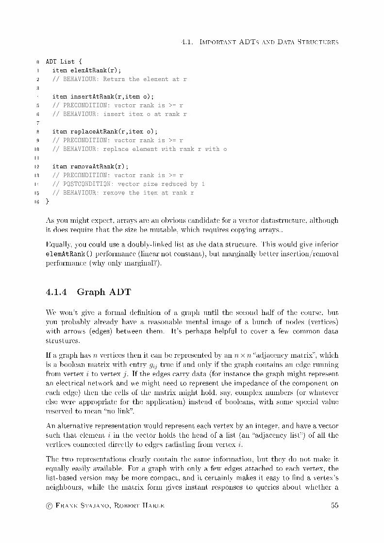
4.1. Important ADTs and Data Structures
0 ADT List
1 item elemAtRank(r);
2 // BEHAVIOUR: Return the element at r
3
4 item insertAtRank(r,item o);
5 // PRECONDITION: vector rank is >= r
6 // BEHAVIOUR: insert item o at rank r
7
8 item replaceAtRank(r,item o);
9 // PRECONDITION: vector rank is >= r
10 // BEHAVIOUR: replace element with rank r with o
11
12 item removeAtRank(r);
13 // PRECONDITION: vector rank is >= r
14 // POSTCONDITION: vector size reduced by 1
15 // BEHAVIOUR: remove the item at rank r
16
As you might expect, arrays are an obvious candidate for a vector datastructure, althoughit does require that the size be mutable, which requires copying arrays..
Equally, you could use a doubly-linked list as the data structure. This would give inferiorelemAtRank() performance (linear not constant), but marginally better insertion/removalperformance (why only marginal?).
4.1.4 Graph ADT
We won't give a formal denition of a graph until the second half of the course, butyou probably already have a reasonable mental image of a bunch of nodes (vertices)with arrows (edges) between them. It's perhaps helpful to cover a few common datastrustures.
If a graph has n vertices then it can be represented by an n×n adjacency matrix, whichis a boolean matrix with entry gij true if and only if the graph contains an edge runningfrom vertex i to vertex j. If the edges carry data (for instance the graph might representan electrical network and we might need to represent the impedance of the component oneach edge) then the cells of the matrix might hold, say, complex numbers (or whateverelse were appropriate for the application) instead of booleans, with some special valuereserved to mean no link.
An alternative representation would represent each vertex by an integer, and have a vectorsuch that element i in the vector holds the head of a list (an adjacency list) of all thevertices connected directly to edges radiating from vertex i.
The two representations clearly contain the same information, but they do not make itequally easily available. For a graph with only a few edges attached to each vertex, thelist-based version may be more compact, and it certainly makes it easy to nd a vertex'sneighbours, while the matrix form gives instant responses to queries about whether a
c© Frank Stajano, Robert Harle 55

Chapter 4. Abstract Data Types and Data structures
random pair of vertices are joined, and can be more compact (especially when there arevery many edges, and if the bit-array is stored in packed form to make full use of machinewords). We shall have much more to say about graphs later in the course.
4.1.5 The Stack ADT
You've met stacks beforethe common mental model is that of a pile of plates, wherethe top is the only accessible element. It is also referred to as LIFO (Last In First Out).Here's the ADT:
0 ADT Stack
1 boolean isEmpty();
2 // BEHAVIOUR: return true iff the structure is empty.
3
4 void push(item x);
5 // BEHAVIOUR: add element <x> to the top of the stack.
6 // POSTCONDITION: isEmpty() == false.
7 // POSTCONDITION: top() == x
8
9 item pop();
10 // PRECONDITION: isEmpty() == false.
11 // BEHAVIOUR: return the element on top of the stack.
12 // As a side effect, remove it from the stack.
13
14
15 item top();
16 // PRECONDITION: isEmpty() == false.
17 // BEHAVIOUR: Return the element on top of the stack (without removing it).
18
In the ADT spirit of specifying the semantics of the data structure using invariants, wemight also add that, for each stack s and for each item x, after the following two-operationsequence
0 s.push(x)
1 s.pop()
the return value of the second statement is x and the stack s is the same as before; butthere are technical problems in expressing this correctly and unambiguously using theabove notation, so we won't try.
The stack ADT given above does not make allowance for the push operation to failalthough, on any real computer with nite memory, it must be possible to do enoughsuccessive pushes to exhaust some resource. This limitation of a practical realization ofan ADT is not deemed a failure to implement the ADT properly: at the level of abstractionof this introductory algorithms course, we do not really admit to the existence of resourcelimits!
There can be various dierent implementations of the Stack data type, but two are espe-cially simple and commonly used. The rst represents the stack as a combination of an
56 Algorithms (20172018)

4.1. Important ADTs and Data Structures
array and an index (pointing to the top of stack, or ToS). The push operation writes avalue into the array and increments the index4, while pop does the converse.
The second representation of stacks is as linked lists, where pushing an item just addsan extra cell to the front of a list, and popping removes it. In both cases the push andpop operations work by modifying stacks in place, so (unlike what might happen in afunctional language such as ML) after invoking either of them the original stack is nolonger available.
Stacks are useful in the most diverse situations. The page description language PostScriptis actually a programming language organized around a stack. In such languages theprogram is a string of tokens that include operands and operators. During programexecution, operands are pushed on the stack; operators pop from the stack the operandsthey require, do their business on them and nally push the result back on the stack. Forexample, the program
3 12 add 4 mul 2 sub
computes (3 + 12) × 4 − 2 and leaves the result, 58, on the stack. This way of writingexpressions is called Reverse Polish Notation and one of its attractions is that it makesparentheses unnecessary (at the cost of having to reorder the expression and making itsomewhat less legible).
4.1.6 The Queue and Deque ADTs
In the Stack ADT, the item removed by the pop() operation was the most recent oneadded by push(). A Queue5 is in most respects similar to a stack, but the rules arechanged so that the item accessed by top() and removed by pop() will be the oldest oneinserted by push() (we shall rename these operations to avoid confusion). Even if ndinga neat way of expressing this in a mathematical description of the Queue ADT may bea challenge, the idea is simple. The above description suggests that stacks and queueswill have very similar interfaces. It is sometimes possible to take an algorithm that usesa stack and obtain an interesting variant by using a queue instead; and vice-versa.
0 ADT Queue
1 boolean isEmpty();
2 // BEHAVIOUR: return true iff the structure is empty.
3
4 void put(item x);
5 // BEHAVIOUR: insert element <x> at the end of the queue.
6 // POSTCONDITION: isEmpty() == false
7
8 item get();
9 // PRECONDITION: isEmpty() == false
10 // BEHAVIOUR: return the first element of the queue, removing it
11 // from the queue.
4Note that stacks growing in the reverse direction are also plausible and indeed frequent. (Why?)5Sometimes referred to as a FIFO, which stands for First In, First Out.
c© Frank Stajano, Robert Harle 57

Chapter 4. Abstract Data Types and Data structures
12
13 item first();
14 // PRECONDITION: isEmpty() == false
15 // BEHAVIOUR: return the first element of the queue, without removing it.
16
17
18
A variant is the perversely-spelt Deque (double-ended queue, pronounced as Dek), whichis accessible from both ends both for insertions and extractions and therefore allows fouroperations:
0 ADT Deque
1 boolean isEmpty();
2
3 void putFront(item x);
4 void putRear(item x);
5 // POSTCONDITION for both: isEmpty() == false
6
7 item getFront();
8 item getRear();
9 // PRECONDITION for both: isEmpty() == false
10
The Stack and Queue may be seen as restricted Deques in which only one put and oneget (as opposed to two of each) are enabled.
4.1.7 The Set and Dictionary ADTs
In this section we're going to look at sets and dictionaries. As you will see, there arelots of similarities and the data structures to implement one is often useful for the others.We'll describe the two ADTs and then look at some data structures useful for either.
Sets
Many algorithms use sets as a building block. Mathematically, a set is an unorderedcollection of distinct objects (so, no duplicates). Sets are very valuable with many uses.An ADT that covered all the operations all would be very large, and so we tend to considervariants that support the operations we want. A starting point might be a static set:
0 boolean isEmpty()
1 // BEHAVIOUR: return true iff the structure is empty.
2
3 boolean hasKey(Key x);
4 // BEHAVIOUR: return true iff the set contains a pair keyed by <x>.
5
6 Key chooseAny();
7 // PRECONDITION: isEmpty() == false
58 Algorithms (20172018)

4.1. Important ADTs and Data Structures
8 // BEHAVIOUR: Return the key of an arbitrary item from the set.
9
10 int size();
11 // BEHAVIOUR: Return the cardinality (size) of the set
Dynamic sets add in the ability to add and remove elements. Whatever you choose veryoften you want to throw in common mathematical operations:
0 Set union (Set s, Set t);
1 // BEHAVIOUR: return the union of sets s and t
2
3 Set intersection(Set s, Set t);
4 // BEHAVIOUR: return the intersection of sets s and t
5
6 Set difference(Set s, Set t);
7 // BEHAVIOUR: Return the difference of sets s and t
8
9 boolean subset(Set s, Set t);
10 // BEHAVIOUR: Return whether set s is a subset of set t
Once again, the ADT says nothing about whether these operations are destructivei.e.whether the set that comes back is a modied version of its inputs or a new Set altogether.Sometimes you get better performance by reusing the inputs for the outputs, but obviouslyyou run the risk that a user of the method doesn't realise this, introducing a bug.
For a more sophisticated variant, it is sometimes useful to assume there is a total orderon the set. Of course, the mathematical denition of a set is an unordered collection,but that doesn't preclude making a set from a collection of element with an order. A setof integers, for example, has a very clear natural ordering, and sometimes it is useful toassume and exploit this. We might add to the ADT:
0 Key min();
1 // PRECONDITION: isEmpty() == false
2 // BEHAVIOUR: Return the smallest key in the set.
3
4 Key max();
5 // PRECONDITION: isEmpty() == false
6 // BEHAVIOUR: Return the largest key in the set.
7
8 Key predecessor(Key k);
9 // PRECONDITION: hasKey(k) == true
10 // PRECONDITION: min() != k
11 // BEHAVIOUR: Return the largest key in the set that is smaller than <k>.
12
13 Key successor(Key k);
14 // PRECONDITION: hasKey(k) == true
15 // PRECONDITION: max() != k
16 // BEHAVIOUR: Return the smallest key in the set that is larger than <k>.
c© Frank Stajano, Robert Harle 59

Chapter 4. Abstract Data Types and Data structures
Dictionaries
Dictionaries associate keys with values and allow you to look up the relevant value if yousupply the key. You met such structures in ML (dictionaries) and Java `(Maps). Theyare also referred to as Tables, Associative arrays or Symbol tables!
Note that, within the dictionary, the mapping between keys and values is a function6: youcannot have dierent values associated with the same key7 . For generality we assumethat keys are of type Key and that values are of type Value. Our ADT is:
0 ADT Dictionary
1 void set(Key k, Value v);
2 // BEHAVIOUR: store the given (<k>, <v>) pair in the dictionary.
3 // If a pair with the same <k> had already been stored, the old
4 // value is overwritten and lost.
5 // POSTCONDITION: get(k) == v
6
7 Value get(Key k);
8 // PRECONDITION: a pair with the sought key <k> is in the dictionary.
9 // BEHAVIOUR: return the value associated with the supplied <k>,
10 // without removing it from the dictionary.
11
12 void delete(Key k);
13 // PRECONDITION: a pair with the given key <k> has already been inserted.
14 // BEHAVIOUR: remove from the dictionary the key-value pair indexed by
15 // the given <k>.
16
Observe that this simple version of the dictionary ADT does not provide a way of askingif some key is in use, and it does not mention anything about the number of items thatcan be stored in a dictionary. Practical implementations must concern themselves withboth these issues.
4.2 Data structures for Sets and/or Dictionaries
There are some very clever data structures and algorithms for handling dierent variantsof sets: those with an order, those that need ecient union, dynamic sets. First we notethat dictionaries are like dynamic sets optimised for lookup, where the keys happen to beassociated with some extra data (values). Given this, a lookup-optimised data structurefor sets will apply to dictionaries. Similarly, a structure for dictionaries can be applied tosets by simply using sentinel (ignored) values.
6As opposed to a generic relation. In other words, only one arrow goes out of each source element.7Sometimes you do want to do this, and languages may oer multimaps or similar. but the ADT
assumes each key is associated with at most one value
60 Algorithms (20172018)

4.2. Data structures for Sets and/or Dictionaries
4.2.1 Vector Representation.
When the keys are known to be drawn from the set of integers in the range 0..n (forsome tractable n), the set/dictionary can be modelled directly by a simple vector, andboth set() and get() operations have unit cost. If the key values come from some otherinteger range (say a..b) then subtracting a from key values gives a suitable index for usewith a vector. This simple and ecient strategy is known as direct addressing. If thenumber of keys actually used is much smaller than the number b−a, direct addressing be-comes extremely inecient (or even infeasible) in space, even though its time performanceremains optimal, namely O(1) worst-case.
4.2.2 Lists
For such sparse sets/dictionaries one could use a list, with each item a record storing akey-value pair. The get() function would scans along the list, searching for the desiredkey. But now there are several options for the set() function. The rst just sticks a newkey-value pair at the front of the list, allowing get() to be coded so as to retrieve the rstvalue that it nds. The second one would scan the list and, if a key was already present,update the associated value in place. If not present it would have to be added. Since inthis second case duplicate keys are avoided, the order in which items in the list are keptwill not aect the correctness of the data type, and so it would be legal (if not alwaysuseful) to make arbitrary permutations of the list each time it was touched.
If one assumes that the keys passed to get() are randomly selected and uniformly dis-tributed over the complete set of keys used, the linked list representation calls for a scandown (an average of) half the length of the list. For the version that always adds anew key-value pair at the head of the list, this cost increases without limit as values arechanged. The other version keeps that cost down but has to scan the list when performingset() operations as well as get()s.
4.2.3 Arrays
Of course we could substitute the list for an array. This gets ugly if keys are deleted ornew ones added, but actually the usage pattern for some applications is to ll a dictionaryat the start and thereafter perform lookups. Then the arry gives us a particular advantageif the keys support an ordering and we sort the array by them. Retrieval is then done viaa binary chop into the array, comparing to the middle of the current range and recursingon the side where the key must be. This means we successively halve the range, givingus a recurrence f(n) = f(n/2) + k, where the k accounts for the comparison cost. Youshould be able to solve this to demonstrate that it is Θ(lg n).
c© Frank Stajano, Robert Harle 61

Chapter 4. Abstract Data Types and Data structures
4.2.4 Binary search trees
TextbookStudy chapter 12 in CLRS3.
A Binary Search Tree (BST) holds a number of keys within a tree structure to helpwith searching. The keys must have a total order (i.e. be sortable). It is a very usefuldata structure to implement dynamic Sets supporting the computation of min(), max(),predecessor() and successor(), and for dictionaries.
Each node of the binary tree will contain an item (consisting of a key-value pair8) andpointers to two sub-trees, the left one for all items with keys smaller than the stored oneand the right one for all the items with larger keys.
Let's look at some interesting operations for BST
Search. Searching such a tree is simple: just compare the sought key with that of thevisited node and, until you nd a match, recurse down in the left or right subtreeas appropriate. The maximum and minimum values in the tree can be found in theleaf nodes discovered by following all left or right pointers (respectively) from theroot. Cost O(height of the tree).
Insertion. Follow the search procedure, moving left or right as appropriate, until youdiscover the key already exists in the tree, or you reach a leaf. Update/Insert there,as appropriate. Cost O(height of the tree).
Deletion. Search to nd the key. If it's a leaf, deletion is trivial. If not, there are variousapproaches you could apply. A non-leaf with only one child can be simply replacedby its child. For a non-leaf with two children, an option is to replace it with itssuccessor (or predecessoreither will work). Then the item for deletion can't havetwo children and can thus be deleted in one of the ways already seen; meanwhile, thenewly moved up object satises the order requirements that keep the tree structurevalid. Cost O(height of the tree).
8If the value takes up more than a minimal amount of space, it is actually stored elsewhere as satellitedata and only a pointer is stored together with the key.
62 Algorithms (20172018)

4.2. Data structures for Sets and/or Dictionaries
Successor9. If a given node has a right subtree then the successor must be in it (why?).If there is no right subtree, the successor might be higher up. Go up to the parent,then grand-parent, then great-grandparent and so on until the link goes up-and-right rather than up-and-left, and you will have the successor. If you reach theroot before having gone up-and-right, then the node has no successor: its key is thehighest in the tree. Cost O(height of the tree).
Rotation. It can be useful to rotate edges around nodes in a BST. A rotation is a localtransformation of a BST that changes the shape of the BST but preserves the BSTpropertiesi.e. you change the tree structure but it's still a valid BST. It's bestseen by examplehere is a right rotation:
Node D changes from being the parent of B to being its right child. A remains B'sleft child and E remains D's right child, but C changes from being B's right childto becoming D's left child. Clearly it could not stay on as B's right child since nowB has acquired D as its new right child! And conversely D has lost its left child(formerly B), so there is a convenient empty space there. A left rotation wouldresverse the whole process.
The end result is another tree, with a slightly dierent shape, but still denitely aBST, as you can easily verify. A and all the other nodes in its subtrees were < B, asB's left child, and still are. E and its subtrees were > D and still are. As for C andits subtree: it used to be > B, as B's right child, but also < D, by virtue of beingwithin B's subtree with B a left child of D. After the rotation, C and its subtree arestill > B, by virtue of having moved into D's subtree, and are < D because they areD's left child. So, with a slight abuse of notation, we can write that A < B < C <D < E holds before and after the rotation.
An important realisation is that the rotation can occur at any node in the tree, notjust the root. Cost-wise, the actual rotation is O(1) since we just exhange a xednumber of pointers.
You will note that, leaving rotations aside, the main operations cost O(height of the tree).The problem with BSTs is that the height depends on the order of insertion of the keys.Insert 1,2,3,4,5 and you get a linear chain of elements, making the height of the tree,equal to the number of elements, n (=5). Insert 3,2,1,4,5 and you get a V-shaped treewith height 3. Insert 2,1,3,4,5 and you get a lop-sided tree with one branch of length 1and one of length 3 (check you agree in all these cases).
As you already know from your studies so far, we want trees to be balanced. In a perfectly-
c© Frank Stajano, Robert Harle 63

Chapter 4. Abstract Data Types and Data structures
balanced tree each branch will be dlg(n)e, which give us our best performance. In theworst case we are unlucky to get a linear list of nodes, with corresponding linear perfor-mance.
So what do you do in practice? One approach is to intelligently apply rotations until youget the most balanced tree possible. This works ne by hand, but coding it up is not fun(by all means, try it). What we really want is to create a data structure that gures thisall out for us...
4.2.5 2-3-4 Trees
In order to make progress with our self-balancing BST, let's take a small detour andlook at a dierent type of tree, which will be helpful in understanding the self-balancingconcept. These other trees are called 2-3-4 trees. They are composed of three dierentnodes: nodes that contain 1 key; nodes that contain 2; and nodes that contain 3. Forreasons that will become clearer later, we will require the number of edges leaving a nodeto be one more than the number of keys it contains. By convention, a node with one keyand two edges is a 2-node, explaining the overall 2-3-4 name. Furthermore, keys arestored in sorted order.
So here is a sketch of our dierent nodes:
In an extension of a BST, each edge points out to a range bounded by the key values, asshown on the diagram above (remember a<b<c since we sort the keys)10. Now, to inserta node with key x we:
1. Walk down the tree, following the edges that contain the key to insert until we getto a leaf node.
2. If the leaf node is a 2- or 3-node, insert x into that node and nish.
3. Else if the leaf node is a 4-node (with, say, keys a, b, c), we rst `explode' it. Themiddle element (c) is moved up a level in the tree, inserting into the parent node ormaking a new root if there is no parent. If we do insert c in the parent and it wasalready a 4-node, we have to explode that node, and so on up the tree11
10I've assumed that all keys are unique. If not, you need to include equality in some of the rangespecications
11Some books have a slightly dierent procedure, where 4-nodes are exploded whenever you passthrough them on the initial walk down the tree. This avoids a walk back up the tree and is simpler to
64 Algorithms (20172018)
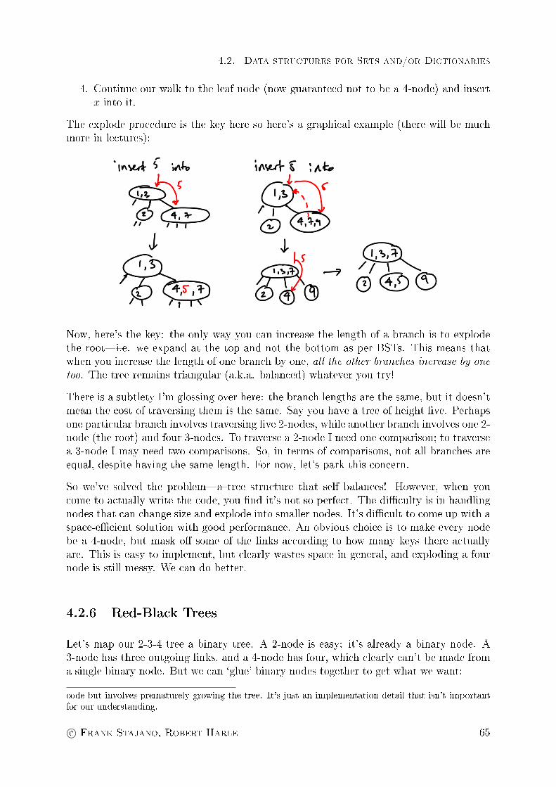
4.2. Data structures for Sets and/or Dictionaries
4. Continue our walk to the leaf node (now guaranteed not to be a 4-node) and insertx into it.
The explode procedure is the key here so here's a graphical example (there will be muchmore in lectures):
Now, here's the key: the only way you can increase the length of a branch is to explodethe rooti.e. we expand at the top and not the bottom as per BSTs. This means thatwhen you increase the length of one branch by one, all the other branches increase by onetoo. The tree remains triangular (a.k.a. balanced) whatever you try!
There is a subtlety I'm glossing over here: the branch lengths are the same, but it doesn'tmean the cost of traversing them is the same. Say you have a tree of height ve. Perhapsone particular branch involves traversing ve 2-nodes, while another branch involves one 2-node (the root) and four 3-nodes. To traverse a 2-node I need one comparison; to traversea 3-node I may need two comparisons. So, in terms of comparisons, not all branches areequal, despite having the same length. For now, let's park this concern.
So we've solved the problema tree structure that self balances! However, when youcome to actually write the code, you nd it's not so perfect. The diculty is in handlingnodes that can change size and explode into smaller nodes. It's dicult to come up with aspace-ecient solution with good performance. An obvious choice is to make every nodebe a 4-node, but mask o some of the links according to how many keys there actuallyare. This is easy to implement, but clearly wastes space in general, and exploding a fournode is still messy. We can do better.
4.2.6 Red-Black Trees
Let's map our 2-3-4 tree a binary tree. A 2-node is easy: it's already a binary node. A3-node has three outgoing links, and a 4-node has four, which clearly can't be made froma single binary node. But we can `glue' binary nodes together to get what we want:
code but involves prematurely growing the tree. It's just an implementation detail that isn't importantfor our understanding.
c© Frank Stajano, Robert Harle 65

Chapter 4. Abstract Data Types and Data structures
I want to use red lines to represent `glue` corresponding to 2-3-4 nodes (and almostcertainly will in lectures), but the notes are in monochrome so I've used double blacklines instead. Here's a 2-3-4 tree and its binary equivalent:
This sort of static mapping is easy: how do we handle additions and enforce the 2-3-4rules like exploding? Actually, just apply the usual BST insertion rules (note our newtree is a BST) and then look for violations. To capture the idea that we always aim toadd to 2-3-4 nodes if we can, we always add a new node using glue edges (red/doublelines).
Take the image above. Let's add 1. In 2-3-4 world we expect the 1 to add to the 0,23-node to give us a 0,1,2 4-node. In BST world we get:
Hmmm. That looks dodgy. If you think about it, we can never get glue edges in directsequence. The glue represents a 2-3-4 node and all of those have black (single) lines
66 Algorithms (20172018)
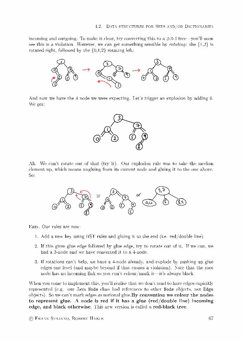
4.2. Data structures for Sets and/or Dictionaries
incoming and outgoing. To make it clear, try converting this to a 2-3-4 treeyou'll soonsee this is a violation. However, we can get something sensible by rotating : the 1,2 isrotated right, followed by the 0,1,2 rotating left:
And now we have the 4-node we were expecting. Let's trigger an explosion by adding 8.We get:
Ah. We can't rotate out of that (try it). Our explosion rule was to take the medianelement up, which means ungluing from its current node and gluing it to the one above.So:
Easy. Our rules are now:
1. Add a new key using BST rules and gluing it to the end (i.e. red/double line).
2. If this gives glue edge followed by glue edge, try to rotate out of it. If we can, wehad a 3-node and we have converted it to a 4-node.
3. If rotations can't help, we have a 4-node already, and explode by pushing up glueedges one level (and maybe beyond if that causes a violation). Note that the rootnode has no incoming link so you can't colour/mark itit's always black.
When you come to implement this, you'll realise that we don't tend to have edges expicitlyrepresented (e.g. our Java Node class had references to other Node objects, not Edge
objects). So we can't mark edges as notional glue.By convention we colour the nodesto represent glue. A node is red if it has a glue (red/double line) incomingedge, and black otherwise. This new version is called a red-black tree.
c© Frank Stajano, Robert Harle 67

Chapter 4. Abstract Data Types and Data structures
Invariants and rules
When you look up red-black trees in most texts, they don't tend to present them as Ido. Most start with a rather mystical set of rules/invariants for a BST used to dene thered-black tree:
1. Every node is either red or black.
2. The root is black.
3. All leaves are black and never contain key-value pairs12.
4. If a node is red, both its children are black.
5. For each node, all paths from that node to descendent leaves contain the samenumber of black nodes.
From our 2-3-4 work we can easily see the origin of these rules:
1. Every node is either red or black.Of courseit's either been glued to another node or it hasn't
2. The root is black.The root has no incoming link (or it would not be the root). So it must be black.
3. All leaves are black and never contain key-value pairs13.We took this for granted in the 2-3-4 tree, and so it applies to the red-black treeequally.
4. If a node is red, both its children are black.This encodes that we can't get glue edge followed by glue edge. This is because thereis no 2-3-4 node with this property, and 2-3-4 nodes are always connected with blacklinks (see next point).
5. For each node, all paths from that node to descendent leaves contain the samenumber of black nodes.A black link in our intermediate tree corresponds directly to a link in the 2-3-4 tree.We know that all paths in the 2-3-4 tree have the same number of nodes, and hencethe same number of black links. Since each glue edge maps to exactly one red node(check it), each black link maps to one black node so the number of black nodes willbe the same along each path.
Analysis
It's tempting to say we have a self-balancing binary tree, so search operations are guar-anteed O(lg n). But it's a bit more subtle. The black height of the tree (the number ofblack nodes along any path) is indeed O(lg n), but a given path could have some number
12Since leaves carry no information, they are sometimes omitted from the drawings; but they arenecessary for the consistency of the remaining invariants.
13Since leaves carry no information, they are sometimes omitted from the drawings; but they arenecessary for the consistency of the remaining invariants.
68 Algorithms (20172018)

4.2. Data structures for Sets and/or Dictionaries
of red nodes that actually unbalance the tree. In lectures we will explore more, but thebottom line is that we can indeed get logarithmic performance.
4.2.7 B-trees
TextbookStudy chapter 18 in CLRS3.
Operating on the trees we've been looking at has us doing two main things: comparisonsor following tree edges. We've been assessing in terms of comparisons, because that'sthe key cost in a system when the data structure is in dynamically instantiated memory(RAM), since following tree edges equates to following pointers, which is all but free.
But data can get big. Too big to be sensibly stored in RAM. Then our data structure mustreside elsewhere. In today's systems that usually means a rotating disc (hard disc) of somesort, and then following tree edges is suddenly more costly than the comparisons. Whatwould our data structure look like if we optimised for fewest disc accesses? Actually, wealready had a hint when we looked at 2-3-4 trees. There we had nodes capable of storingmore data, meaning fewer edges in the graph compared to the BST equivalent. So let'sgo further now: make the nodes big enough to take lots of keys. This leads us to B-trees,of which 2-3-4 trees are a special case. The B-tree rules are:
1. There are internal nodes (with keys and payloads and children) and leaf nodes(without keys or payloads or children).
2. For each key in a node, the node also holds the associated payload14.
3. All leaf nodes are at the same distance from the root.
4. All internal nodes have at most 2t children; all internal nodes except the root haveat least t children.
5. A node has c children i it has c− 1 keys.
We can immediately see this as generalising our 2-3-4 trees. Rules 1 and 2 are the same.Rule 5 says the number of children (outgoing edges) is equal to one more than the numberof keys so we know what partition of the key range an edge represents. Rule 3 is justsaying the tree is balanced in terms of eight, which we knew from 2-3-4 analysis.
Rule 4 is the only one that perhaps isn't obvious. We can see that t = 2 holds for a2-3-4 tree, but that isn't enough: why the minimum and maximum specied? One wayto see why is to consider exploding a node. To explode it would need to be fulli.e. have(2t− 1) keys and 2t children. The median value will go up a level, cleaving the remainingkeys into two nodes each with (t− 1) keys and t children. Exploding is the only way wecan create new nodes so what this tells us is there is no way to have fewer than (t − 1)or more than 2t− 1 keys, giving us rule 4. Note that the root must be exempt from theminimum in this rule, else how could you ever represent data with fewer than t− 1 keys.
14Or, more likely, a pointer to it, unless the payload has a small xed size comparable to that of thepointer.
c© Frank Stajano, Robert Harle 69
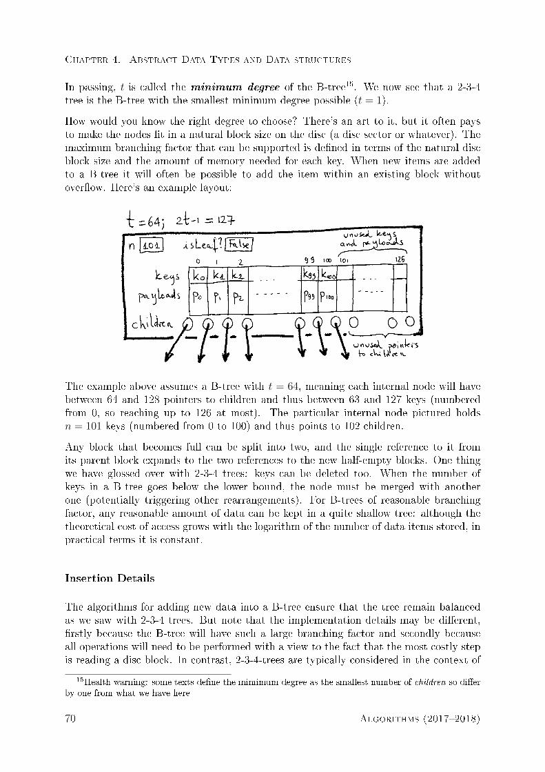
Chapter 4. Abstract Data Types and Data structures
In passing, t is called the minimum degree of the B-tree15. We now see that a 2-3-4tree is the B-tree with the smallest minimum degree possible (t = 1).
How would you know the right degree to choose? There's an art to it, but it often paysto make the nodes t in a natural block size on the disc (a disc sector or whatever). Themaximum branching factor that can be supported is dened in terms of the natural discblock size and the amount of memory needed for each key. When new items are addedto a B-tree it will often be possible to add the item within an existing block withoutoverow. Here's an example layout:
The example above assumes a B-tree with t = 64, meaning each internal node will havebetween 64 and 128 pointers to children and thus between 63 and 127 keys (numberedfrom 0, so reaching up to 126 at most). The particular internal node pictured holdsn = 101 keys (numbered from 0 to 100) and thus points to 102 children.
Any block that becomes full can be split into two, and the single reference to it fromits parent block expands to the two references to the new half-empty blocks. One thingwe have glossed over with 2-3-4 trees: keys can be deleted too. When the number ofkeys in a B-tree goes below the lower bound, the node must be merged with anotherone (potentially triggering other rearrangements). For B-trees of reasonable branchingfactor, any reasonable amount of data can be kept in a quite shallow tree: although thetheoretical cost of access grows with the logarithm of the number of data items stored, inpractical terms it is constant.
Insertion Details
The algorithms for adding new data into a B-tree ensure that the tree remain balancedas we saw with 2-3-4 trees. But note that the implementation details may be dierent,rstly because the B-tree will have such a large branching factor and secondly becauseall operations will need to be performed with a view to the fact that the most costly stepis reading a disc block. In contrast, 2-3-4-trees are typically considered in the context of
15Health warning: some texts dene the mimimum degree as the smallest number of children so dierby one from what we have here
70 Algorithms (20172018)

4.2. Data structures for Sets and/or Dictionaries
in-memory data structures so you count memory accesses rather than disc accesses whenevaluating and optimizing an implementation.
So: to insert a new key (and payload) into a B-tree, look for the key in the B-tree in theusual way. If found, update the payload in place. If not found, you'll be by then in theright place at the bottom level of the tree (the one where nodes have keyless leaves aschildren); on the way down, whenever you nd a full node, split it in two on the mediankey and migrate the median key and resulting two children to the parent node (which byinductive hypothesis won't be full). If the root is full when you start, split it into threenodes (yielding a new root with only one key and adding one level to the tree). When welooked at 2-3-4 trees, we chose not to split pre-emptively, but rather to work back up thetree in a chain reaction of explosions when it occurred. Here we split as we go becausethe cost of going back to previous nodes is very high (it's another big disc seek). Onceyou get to the appropriate bottom level node, which won't be full or you would have splitit on your way there, insert there.
Deletion details
Deleting is a more elaborate aair because it involves numerous subcases. You can't deletea key from anywhere other than a bottom node (i.e. one whose children are keyless leaves),otherwise you upset its left and right children that lose their separator. In addition,you can't delete a key from a node that already has the minimum number of keys. Sothe general algorithm consists of creating the right conditions and then deleting (or,alternatively, deleting and then readjusting).
To move a key to a bottom node for the purpose of deleting it, swap it with its successor.This must be in a bottom node by the following reasoning:
After the swap the tree will have a temporary inversion, but that will disappear as soonas the unwanted key is deleted.
To rell a node that has too few keys, use an appropriate combination of the followingthree operations, which rearrange a local part of a B-tree in constant time preserving allthe B-tree properties.
Merge The rst operation merges two adjacent brother nodes and the key that separatesthem from the parent node. The parent node loses one key.
Split The reverse operation splits a node into three: a left brother, a separating key anda right brother. The separating key is sent up to the parent.
Redistribute The last operation redistributes the keys among two adjacent sibling nodes.It may be thought of as a merge followed by a split in a dierent place16, and thisdierent place will typically be the centre of the large merged node.
Each of these operations is only allowed if the new nodes thus formed respect their minand max capacity constraints. Here is then the pseudocode algorithm to delete a key k
16We say thought of because such a merge might be disallowed as a stand-alone B-tree operationtheresulting node might end up having more than the allowed number of keys.
c© Frank Stajano, Robert Harle 71

Chapter 4. Abstract Data Types and Data structures
from the B-tree.
0 def delete(k):
1 """B-tree method for deleting key k.
2 PRECONDITION: k is in this B-tree.
3 POSTCONDITION: k is no longer in this B-tree."""
4
5 if k is in a bottom node B:
6 if B can lose a key without becoming too small:
7 delete k from B locally
8 else:
9 refill B (see below)
10 delete k from B locally
11 else:
12 swap k with its successor
13 # ASSERT: now k is in a bottom node
14 delete k from the bottom node with a recursive invocation
The following pseudocode, invoked as a subroutine by the previous fragment, rells a nodeB that currently has the minimum allowed number of keys.
0 def refill(B):
1 """B-tree method for refilling node B.
2 PRECONDITION: B is an internal node of this B-tree, with t-1 keys.
3 POSTCONDITION: B now has more than t-1 keys."""
4
5 if either the left or right sibling of B can afford to lose any keys:
6 redistribute keys between B and that sibling
7 else:
8 # ASSERT: B and its siblings all have the min number of keys, t-1
9 merge B with either of its siblings
10 # ...this may require recursively refilling the parent of B,
11 # because it will lose a key during the merge.
4.2.8 Hash tables
TextbookStudy chapter 11 in CLRS3.
A hash table implements the general case of the Dictionary ADT, where keys may nothave a total order dened on them. In fact, even when the keys used do have an orderrelationship associated with them, it may be worth looking for a way of building a dictio-nary without using this order. Binary search makes locating items in a dictionary easierby imposing a coherent and ordered structure; hashing, instead, places its bet the otherway, on chaos.
A hash function h(k) maps a key of arbitrary length onto an integer in the range 0 tom−1for some size m and, for a good hash function, this mapping will appear to have hardlyany pattern. Now, if we have an array of size m, we can try to store a key-value pair with
72 Algorithms (20172018)
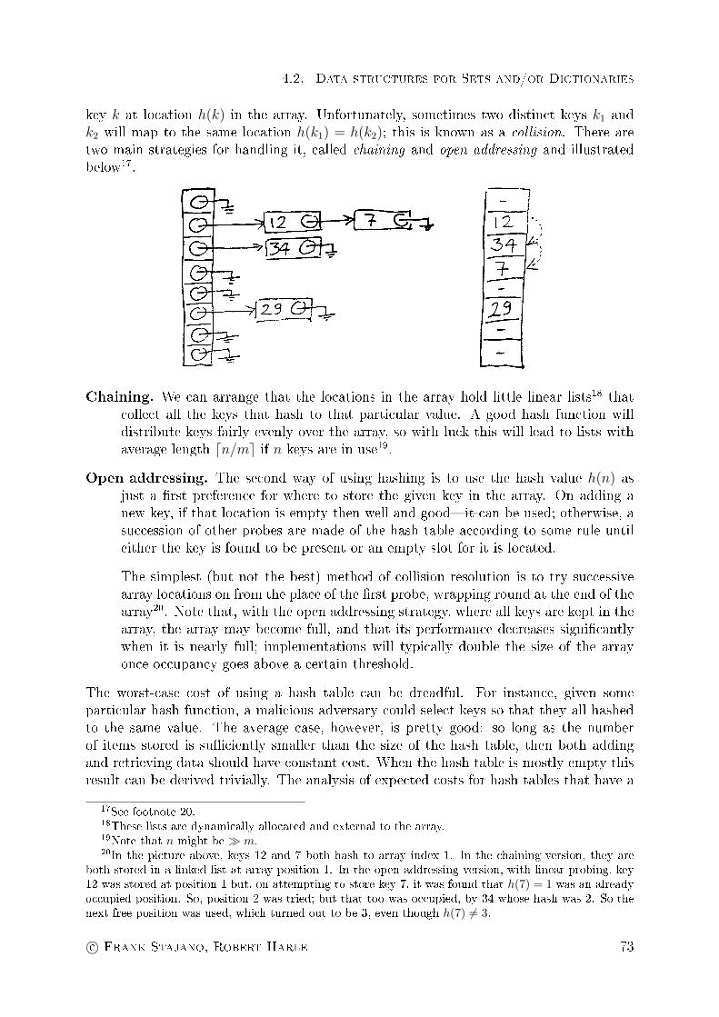
4.2. Data structures for Sets and/or Dictionaries
key k at location h(k) in the array. Unfortunately, sometimes two distinct keys k1 andk2 will map to the same location h(k1) = h(k2); this is known as a collision. There aretwo main strategies for handling it, called chaining and open addressing and illustratedbelow17.
Chaining. We can arrange that the locations in the array hold little linear lists18 thatcollect all the keys that hash to that particular value. A good hash function willdistribute keys fairly evenly over the array, so with luck this will lead to lists withaverage length dn/me if n keys are in use19.
Open addressing. The second way of using hashing is to use the hash value h(n) asjust a rst preference for where to store the given key in the array. On adding anew key, if that location is empty then well and goodit can be used; otherwise, asuccession of other probes are made of the hash table according to some rule untileither the key is found to be present or an empty slot for it is located.
The simplest (but not the best) method of collision resolution is to try successivearray locations on from the place of the rst probe, wrapping round at the end of thearray20. Note that, with the open addressing strategy, where all keys are kept in thearray, the array may become full, and that its performance decreases signicantlywhen it is nearly full; implementations will typically double the size of the arrayonce occupancy goes above a certain threshold.
The worst-case cost of using a hash table can be dreadful. For instance, given someparticular hash function, a malicious adversary could select keys so that they all hashedto the same value. The average case, however, is pretty good: so long as the numberof items stored is suciently smaller than the size of the hash table, then both addingand retrieving data should have constant cost. When the hash table is mostly empty thisresult can be derived trivially. The analysis of expected costs for hash tables that have a
17See footnote 20.18These lists are dynamically allocated and external to the array.19Note that n might be m.20In the picture above, keys 12 and 7 both hash to array index 1. In the chaining version, they are
both stored in a linked list at array position 1. In the open addressing version, with linear probing, key12 was stored at position 1 but, on attempting to store key 7, it was found that h(7) = 1 was an alreadyoccupied position. So, position 2 was tried; but that too was occupied, by 34 whose hash was 2. So thenext free position was used, which turned out to be 3, even though h(7) 6= 3.
c© Frank Stajano, Robert Harle 73

Chapter 4. Abstract Data Types and Data structures
realistic load is of course more complex but, so long as the hash table isn't too close tobeing full, we still get constant-time performance for the average case.
A short note on terminology
Confusingly, some people (not us) use the terms open hashing to refer to chainingand closed hashing to refer to open addressingbe ready for it. But we shall insteadconsistently use the terminology in CLRS3, as indicated above.
Probing sequences for open addressing
Many strategies exist for determining the sequence of slots to visit until a free one isfound. We may describe the probe sequence as a function of the key k and of the attemptnumber j (in the range from 0 to m−1). Using a Java-like pseudocode to show argumenttypes:
0 int probe(Key k, int j);
1 // BEHAVIOUR: return the array index to be probed at attempt <j>
2 // for key <k>.
So as not to waste slots, the curried function obtained by xing the key to any constantvalue must be a permutation of 0, . . . ,m − 1 (the range of indices of the array). Inother words, we wish to avoid probe sequences that, for some keys, fail to explore someslots.
Linear probing This easy probing function just returns h(k) + j mod m. In otherwords, at every new attempt, try the next cell in sequence. It is always a permutation.Linear probing is simple to understand and implement but it leads to primary clustering :many failed attempts hit the same slot and spill over to the same follow-up slots. Theresult is longer and longer runs of occupied slots, increasing search time.
Quadratic probing With quadratic probing you return h(k) + cj + dj2 mod m forsome constants c and d. This works much better than linear probing, provided that cand d are chosen appropriately: when two distinct probing sequences hit the same slot,in subsequent probes they then hit dierent slots. However it still leads to secondaryclustering because any two keys that hash to the same value will yield the same probingsequence.
Double hashing With double hashing the probing sequence is h1(k)+ j ·h2(k) mod m,using two dierent hash functions h1 and h2. As a consequence, even keys that hash tothe same value (under h1) are in fact assigned dierent probing sequences. It is the bestof the three methods in terms of spreading the probes across all slots, but of course eachaccess costs an extra hash function computation.
74 Algorithms (20172018)

4.3. Priority queue ADT
How should the probing sequence be used? The get(), set() and delete() methods allneed rst to determine the array slot to read from, write to or delete respectively. To dothat, they keep calling the probing function until they reach the correct slot or until theyhave tried m times unsuccessfully.
In the case of get(), the correct slot is the rst one in the sequence that contains thesought key; and if an empty slot is found along the way, then the key is not in thedictionary even if fewer than m probes have been attempted.
In the case of set(), if a slot with the sought key is found, that's the one to use, andwe are overwriting a previous value for the same key; otherwise, the rst empty slot inthe probing sequence should be used, and we'll be setting a value for this key for the rsttime. If m probes are all unsuccessful, then the array is full and insertion cannot takeplace without rst resizing it.
In the case of deletion, there are complications. Assuming that we found the slot with thekey to be deleted, if we naïvely marked it as empty we would be potentially interruptingsome chains and making it impossible for get() to reach any stored keys whose probingsequence had that slot in a previous position. What we need to do is mark the slot asdeleted (a special value distinct from empty) and change the implementations of get()and set() to treat the deleted value appropriately (treating it like non-empty for get()but like empty for set()).
Unfortunately, even with this x, one moment's thought shows that a long sequence ofset() and delete() operations will eventually result in the array running out of emptyslots even though many may be marked deleted. As a result, the get() operation willbecome slower and slower (because chains of deleted slots need to be traversed until thesought value is found or an empty cell is reached) until, in the limit, all unsuccessfulsearches will cost m probes. This is of course unacceptable and therefore, when a dictio-nary must support deletions, it should either be implemented with chaining or, in case ofopen addressing, it should be rehashed well before it runs out of empty cells.
Rehashing a dictionary consists of creating a new array (usually twice as large, to amortizethe cost of the operation; clearly with a new hash function, since the index range isdierent), inserting every key-value pair of the old array into the new one and deletingthe old array. Deleted slots are not copied and are therefore implicitly transformed intoempty ones. Even without deletions, the resizing and rehashing procedure is also necessaryto preserve performance when the load factor (array cells in use divided by array cellsavailable) becomes too high, simply as a consequence of too many insertions for the sizeof the array. In the HashMap data structure supplied with the Java library, for example,by default a rehash is triggered when the load factor reaches 75%.
4.3 Priority queue ADT
TextbookStudy chapter 6 in CLRS3.
c© Frank Stajano, Robert Harle 75

Chapter 4. Abstract Data Types and Data structures
If we concentrate on the operations set(), min() and delete(), subject to the extracondition that the only item we ever delete will be the one just identied as the minimumone in our set, then the data structure we have is known as a priority queue. Asthe name says, this data structure is useful to keep track of a dynamic set of clients(e.g. operating system processes, or graph edges), each keyed with its priority, and havethe highest-priority one always be promoted to the front of the queue, regardless of whenit joined. Another operation that this structure must support is the promotion of anitem to a more favourable position in the queue, which is equivalent to rewriting the keyof the item.
A priority queue is thus a data structure that holds a dynamic set of items and oersconvenient access to the item with highest priority21, as well as facilities for extractingthat item, inserting new items and promoting a given item to a priority higher than itscurrent one.
0 ADT PriorityQueue
1 void insert(Item x);
2 // BEHAVIOUR: add item <x> to the queue.
3
4 Item first(); // equivalent to min()
5 // BEHAVIOUR: return the item with the smallest key (without
6 // removing it from the queue).
7
8 Item extractMin(); // equivalent to delete(), with restriction
9 // BEHAVIOUR: return the item with the smallest key and remove it
10 // from the queue.
11
12 void decreaseKey(Item x, Key new);
13 // PRECONDITION: new < x.key
14 // PRECONDITION: Item <x> is already in the queue.
15 // POSTCONDITION: x.key == new
16 // BEHAVIOUR: change the key of the designated item to the designated
17 // value, thereby increasing the item's priority (while of course
18 // preserving the invariants of the data structure).
19
20 void delete(Item x);
21 // PRECONDITION: item <x> is already in the queue.
22 // BEHAVIOUR: remove item <x> from the queue.
23 // IMPLEMENTATION: make <x> the new minimum by calling decreaseKey with
24 // a value (conceptually: minus infinity) smaller than any in the queue;
25 // then extract the minimum and discard it.
26
27
28 ADT Item
29 // A total order is defined on the keys.
30 Key k;
31 Payload p;
21Highest priority by convention means earliest in the sorting order and therefore numericallysmallest in case of integers. Priority 1 is higher than priority 3.
76 Algorithms (20172018)

4.3. Priority queue ADT
32
As for implementation, you could simply use a sorted array, but you'd have to keep thearray sorted at every operation, for example with one pass of bubble-sort, which giveslinear time costs for any operations that change the priority queue.
Operation Cost with sorted arraycreation of empty queue O(1)first() O(1)insert() O(n)extractMin() O(n)decreaseKey() O(n)delete() O(n)
But we can do better than this.
4.3.1 Binary heaps
A good representation for a priority queue is the binary heap, which is the data structureimplicitly used in the heapsort algorithm22 of section 2.13. It is a clever yet comparativelysimple construction that allows you to read out the highest priority item in constant timecost (if you don't remove it from the queue) and lets you achieve O(lg n) costs for allother priority queue operations.
A min-heap is a binary tree that satises two additional invariants: it is almost full(i.e. all its levels except perhaps the lowest have the maximum number of nodes, and thelowest level is lled left-to-right) and it obeys the heap property whereby each node hasa key less than or equal to those of its children.
As a consequence of the heap property, the root of the tree is the smallest element.Therefore, to read out the highest priority item, just look at the root (constant cost).To insert an item, add it at the end of the heap and let it bubble up (following parentpointers) to a position where it no longer violates the heap property (max number of steps:
22Except that heapsort uses a max-heap and here we use a min-heap.
c© Frank Stajano, Robert Harle 77

Chapter 4. Abstract Data Types and Data structures
proportional to the height of the tree). To extract the root, read it out, then replace itwith the element at the end of the heap, letting the latter sink down until it no longerviolates the heap property (again the max number of steps is proportional to the heightof the tree). To reposition an item after decreasing its key, let it bubble up towards theroot (again in no more steps than the height of the tree, within a constant factor).
Since the tree is balanced (by construction, because it is always almost full), its heightnever exceeds O(lg n), which is therefore the asymptotic complexity bound on all thepriority queue operations that alter the tree.
Operation Cost with binary min-heapcreation of empty heap O(1)first() O(1)insert() O(lg n)extractMin() O(lg n)decreaseKey() O(lg n)delete() O(lg n)
These logarithmic costs represent good value and the binary heap, which is simple tocode and compact to store23, is therefore a good choice, in many cases, for implementinga priority queue.
23The array representation does not even require any extra space for pointers.
78 Algorithms (20172018)