aircraft flight dynamics with simulated ice...

c)2001 American Institute of Aeronautics & Astronautics or Published with Permission of Author(s) and/or Author(s)' Sponsoring Organization.

mmm mm fm_ ********—— =. ______________ A01-16413

AIAA-2001-0541Aircraft Flight Dynamics with Simulated IceAccretionD. Pokhariyal, M.B. Bragg, T. Hutchison, and J. MerretUniversity of Illinois at Urbana-ChampaignUrbana, Illinois

39th AIAA Aerospace SciencesMeeting & Exhibit

8-11 January 2001 / Reno, NVFoyDermission to copy or republish, contact the American Institute of Aeronautics and Astronautics1801 Alexander Bell Drive, Suite 500, Reston, VA 20191


Aircraft Flight Dynamics with Simulated Ice Accretion

Devesh Pokhariyal,* Michael B. Bragg,* Tim Hutchison,A and Jason Merret*

University of Dlinois at Urbana-Champaign

ABSTRACT

The effect of ice accretion on aircraft performance andcontrol during trim conditions was modeled andanalyzed. A six degree-of-freedom computationalflight dynamics model was used to study the effect ofice accretion on the aircraft dynamics. The effects ofturbulence and sensor noise were modeled and filterswere developed to remove unwanted noisy data withoutaffecting the short period and phugoid modes. Thisstudy is part of a larger research program to developsmart icing system technology. The goal of the studyreported here was to develop techniques to sense theeffect and location of ice accretion on aircraftperformance and control during trimmed flight.Control surface steady and unsteady hinge-momentswere modeled as a potential aerodynamic performancesensor. Microburst and gravity wave atmosphericdisturbances were modeled and their effects on theaircraft performance and control were compared to thatof an icing encounter. The simulations showed thatatmospheric disturbances could be differentiated fromicing encounters. The hinge-moment sensors provedvery useful in identifying the wing versus tail locationof aircraft icing.

LIST OF SYMBOLS AND ABBREVIATIONS

C(A) arbitrary performance or stability andcontrol derivative

Q airfoil drag coefficientCh hinge-moment coefficientCH, RMS unsteady hinge-moment coefficientCi lift coefficientCm pitching moment coefficient

Fx, Fy, Fz forces on the aircraftFDC Flight Dynamics Codeg(n) freezing fraction effect on dragh altitudeIMS Ice Management SystemIPS Icing Protection SystemkCA coefficient icing factor constant

kc coefficient icing factorLWC Liquid Water ContentMVD Median Volumetric Diameterm aircraft massn freezing fractionp, q, r aircraft angular velocitiesqg effective pitch rate due to gust velocityr radial coordinateR microburst radiusSIS Smart Icing SystemT temperaturet timeTIP Tailplane Icing Programu, v, w atmospheric velocitiesV aircraft, freestream velocityx, y, z rectangular coordinatesZi,2,3 drag equation constantsz* characteristic height out of the boundary

layerA changea angle of attack5e elevator deflectionA microburst constant77 aircraft icing parameterr/ice icing severity parameter

* Graduate Research Assistant, Department of Aeronautical and Astronautical Engineering, currentlyAerospace/Simulation Engineer, NLX Corporation, Sterling, VA, Member AIAA.f Professor and Head, Department of Aeronautical and Astronautical Engineering, Associate Fellow AIAA.

Graduate Research Assistant, Department of Aeronautical and Astronautical Engineering, currently AeronauticalEngineer, Naval Air Warfare Center - Aircraft Division, Patuxent River, MD, Member AIAA.* Graduate Research Assistant, Department of Aeronautical and Astronautical Engineering, Member AIAA.

Copyright 2001 © by Michael B. Bragg. Published by American Institute of Aeronautics and Astronautics, Inc.with permission.

American Institute of Aeronautics and Astronautics


1.0 INTRODUCTION

The research presented in this paper was acontinuation of the work presented by Bragg et al.1Recent commuter aircraft icing accidents highlight theneed for improved safety. The primary cause of theseaccidents was the effect of ice on aircraft control.2With a projected growth in airline traffic, the need toaddress aircraft icing and its effects on aircraft handlingqualities is apparent. As mentioned by Bragg et al.,1icing accidents can be prevented in two different ways:1) icing conditions can be avoided, or 2) the aircraftsystem can be designed and operated in an ice tolerantmanner. For all aircraft, ice avoidance is a desirablegoal for increased safety. However, for commercialaircraft, where revenue and schedules must bemaintained, ice tolerance will continue to be thepreferred method for all but the most severe icingconditions. Our approach is to conduct research toimprove the safety of operations in icing conditions (icetolerance) by developing the Smart Icing Systems (SIS)concept.

In this paper, a simple model is presented toinclude the effect of ice on linear and nonlinear aircraftstability and control derivatives. A more accuratemodel based on a neural network approach is alsodiscussed. This technique is used in conjunction with asix degree-of-freedom computational flight mechanicsmodel to study the effects of ice on aircraft dynamics.Control surface hinge-moments are evaluated forpossible use in detecting the effect and location of iceaccretion in flight when insufficient dynamic content,such as the vehicle response to an elevator doublet, isavailable to use system identification techniques. Muchresearch has been conducted to determine the effect ofice on performance and handling qualities, howeverother phenomena, such as atmospheric disturbance canpotentially cause similar effects. Research is presentedhere on aircraft microburst and gravity wave encountersto understand how those can be identified to eliminatefalse alarms.

2.0 THEORETICAL AND COMPUTATIONALMETHODS

2.1 Iced Aircraft Model Development

A simple, but physically representative, model of theeffect of ice on aircraft flight mechanics is used in thispaper. The method was described in detail in aprevious paper1 and will only be reviewed here andsome recent improvements presented. The icing effectsmodel is based on the following equation

(A)iced ~~ ( * "*" tfice

In this equation, rjice is an icing severity parameter, andrepresents the amount and severity of the icingencounter. rjice is defined such that it is not a functionof the aircraft, only the atmospheric conditions. k'c isthe coefficient icing factor that depends the coefficientbeing modified and the aircraft specific information.Here the k'c term accounts for one aircraft due to itssize, speed, or design being more susceptible to icingthan another aircraft. C(A) is any arbitrary performance,stability or control parameter or derivative that isaffected by ice accretion.

In this formulation, the weighting factor, k'c , isassumed to be

i,' _ i ,,

Here the term rjice is the ratio of the drag rise on aNACA 0012 airfoil at the current icing cloud conditionsto the drag rise experienced at a reference condition inthe continuous maximum icing envelope. The equationfor rjice is

= &Cd(NACA 0012,c = 3',V = ll5kts,actuaLconditions)AQre (NACA 0012, c = 3\cont. max.conditions)

The rjice value is calculated as above, using a three-foot chord NACA 0012 airfoil at 175 knots. Here 77,the aircraft icing parameter, is calculated in the sameway as rjice except the chord and velocity correspondingthe aircraft and conditions being examined are used inthe numerator. The kCA represents the change in anaircraft parameter CA , that is constant for a givenaircraft. By using this formulation, the aircraft specificchord, airfoil, and velocity are adequately captured,allowing for a more accurate determination of icedcoefficient values.

Recently the iced aircraft model has undergonesome minor refinements. The database of icing casesused to define the model was expanded to include 115distinct icing cases that were extracted from data takenat the NASA Lewis Icing Research Tunnel andpresented in three separate NASA TechnicalMemorandums.3"5 Approximately 86% of these caseswere based on the NACA 0012 airfoil, and theremaining 14% were based on the NACA 63(2)-A415airfoil.



The equation for the ACd curves has the followinggeneral form for t < 10 minutes:

Where Z; is a constant, and the function g varies ina nonlinear fashion with n, peaking at a value of 0.2.As before, the ACd curves were constructed to varylinearly with the value of ACE (and time) until the timeof the encounter reached 10 minutes. Once the lengthof the icing encounter exceeded ten minutes, a linearvariation with time was no longer representative of theactual drag increase. Since approximately only 10% ofthe cases in the database provided data for encountersbeyond ten minutes, the formulation for long timeencounters was estimated. Once beyond the ten minutethreshold, the ACd increase was estimated to decayexponentially to a point that was twice the ACd value atten minutes. The general form of the ACd equation for t> 10 minutes was as follows:

ACd=Z2-(l-eZ3 ' '°)+ACd (at 10 minutes)

Where Z2 and Z3 are constants based in part on thecalculated value of ACd at ten minutes, and t10 is thetime elapsed after the passage of the ten-minute mark.

2.2 Neural Net Development

The correlations between atmospheric conditions,ice shapes and aircraft stability and control derivativesare very complex. In an attempt to develop an initialrelationship between ice shapes and aerodynamiccoefficients, neural networks have been implementedon recent experimental data to determine if arelationship could be found.

An excellent definition of a neural network wasgiven by Haykin.6 "A neural network is a massivelyparallel distributed processor made up of simpleprocessing units, which has a natural propensity forstoring experiential knowledge and making it availablefor use." Neural networks are loosely based on thestructure of the human brain. Figure 1 is a schematicdiagram of a neural network with four inputs and fouroutputs. There are several hidden layers ofinterconnected nodes within the neural network thattake the provided inputs, multiply them by "synapticweights," and then output the results either to anotherhidden layer or the output layer. The values of thesynaptic weights are determined by training the neuralnetwork with known correlations. The synaptic weightsof the nodes in a neural network can be linear or

nonlinear, and as such, neural networks are excellent inhandling nonlinear data. There are many differentapplications for neural networks, one of which isfinding correlations within complex sets of data. In thisresearch, neural networks have been used in thismanner as a powerful curve-fitting tool, attempting tocorrelate the characteristics of ice shapes toaerodynamic variables.

The data used for this exploration were taken froma paper by Kim and Bragg.7 These data provide the C,,Q, Cm and Ch for a NLF-0414 airfoil with threedifferent simulated glaze ice horn heights and sixdifferent locations over a range of angles of attack. Thedata also contain the effect of three different horn basewidths and three different horn leading-edge radii. Thevariations of these values resulted in a database of1,740 separate data points.

Using the Matlab Neural Network Toolbox,different neural nets were created using the 1,740 datapoints. During the training, the neural network looks ateach data point individually, and attempts to adjust thesynaptic weight of each node such that the inputs resultin an output that is close to the known data. Eachanalysis of the entire data set is referred to as an epoch.For these networks, the Neural Network Toolbox wasprogrammed to stop training after 500 epochs.Generally, the largest reduction in the error of thenetwork occurs well before the first 150 epochs, afterwhich there is very little increase in the accuracy of thenetwork. This behavior is common when using neuralnets to find trends in data, although the number ofepochs to reach a reduction in error can varysignificantly.

Each network consisted of five input nodes (angleof attack, horn location, horn height, horn base widthand horn leading edge radius) and four output nodes(C/, Cm, Cd and Q). Several nets were trained, seekingthe optimum configuration of hidden layers and nodesthat provided the best correlation between experimentaland "simulated" (within the neural net) data. Due to thelarge amount of data and epochs, training the neuralnets took several hours on a 450 MHz Pentium-classprocessor, and as such, the training time was consideredwhen choosing a network for the simulations. Thecurrent network being used in the simulations consist offive hidden layers often nodes each.

Initially, the neural networks were trained using allof the available data to determine if a correlation couldbe found between the ice shape parameters andaerodynamic coefficients. Once it was determined thata correlation existed, it was required to determinewhether the neural net was able to predict values thatwere not in its training set. To this end, the neural netswere then retrained using only half of the available



data. This allows for a direct comparison between thenetwork's simulated data and the unused experimentaldata.

Using the neural networks to determine thepossible relationships between ice shapes andaerodynamic performance was only an initial step in aproposed chain of neural networks. Future researchwill test and develop two other sets of neural networks.One set would predict ice shapes based on the icingcloud parameters and aircraft information, while theother set would determine three-dimensionalaerodynamic coefficients based on the two-dimensionalcoefficients. Combined with the neural networksdescribed in this paper, these two additional sets wouldallow for a series of neural networks that would be ableto relate environmental ice accretion parameters tothree-dimensional aerodynamic coefficients andstability and control derivatives.

2.3 Clean and Iced Aircraft Models

The current longitudinal and lateral aircraft flightdynamics model was obtained from published NASATwin Otter flight results. The results obtained from theTwin Otter flight with simulated tailplane icing wereused to estimate most of the derivatives.8'9 The drag andother non-tail related derivatives were obtained fromflight test results in which the entire aircraft wassubjected to icing.10 Where values were not available,they were estimated. A comparison of the clean andiced derivatives is shown in Table 1. Also shown is asimple model of horizontal tail icing only and wingicing only, derived from these same data. Thederivatives are representative of icing conditions thatyield 77= 0.0675. This model was intended primarilyfor use in the trimmed flight analysis performed in thispaper.

2.4 Flight Mechanics Code

The flight analysis of the clean and iced aircraftmodels were carried out using the Flight Dynamics andControl (FDC) toolbox for MATLAB & Simulink.11

The FDC code solves 12-coupled nonlinear differentialequations to describe the aircraft's dynamic motionusing control surface deflections, power, etc. as inputs.The FDC also incorporates an atmospheric turbulencemodel based on the NASA Dryden wind gust model.The onset and accumulation of icing are modeledduring flight in the FDC code by modifying theaerodynamic derivatives at each time step as describedby Bragg et al.1 Various flight models can beincorporated into the FDC code and used to simulate

aircraft dynamics. The FDC code is modified asrequired and simulations are carried out in the openloop and autopilot modes. The code has also beenupdated to include sensor noise, microbursts andaerodynamic hinge-moment calculations.

A validation of the FDC code was carried out, byBragg et al.,1 where results obtained using the FDCwere compared to those obtained by the method ofMiller and Ribbens12 and the NASA TIP flight p5220.

The effects of turbulence and sensor noise wereincorporated into the FDC code as described in thepaper by Bragg et.al.1 Filters to remove unwanted noisydata without affecting the short period and phugoidmodes were also developed.1

2.5 Hinge-Moment Measurements

Ice accretion on surfaces such as the leading edgesof the wing and tail have a direct influence on the liftgeneration and the controllability of an aircraft. Theeffect of such ice build-up requires different recoverymethods as shown by Ratvasky et al.13 Non-uniformaircraft icing can result due to non uniform shedding aswell as selective ice protection operation, or a failure.The many control related aircraft icing accidentshighlight the importance of identifying icing-relatedcontrol problems. The formation of ice on airfoilsurfaces often results in a separation bubble, whichseverely alters the surface pressure distribution. On-board hinge-moment sensors were explored as a meansto determine the effects of icing on different aircraftcontrol surfaces.

Gurbacki and Bragg14 measured hinge-moment, Q,and unsteady hinge-moments, ChtRMSl on a NACA23012 airfoil with a flap. Data were collected forforward facing quarter round ice shapes placed atdifferent x/c locations while varying the angle of attackand flap deflection. The hinge-moment measurementsand the fluctuation of the hinge-moment (the unsteadyrms value) capture the effects of icing on the flow fieldover the airfoil surface.

The results from Gurbacki and Bragg14 showed thatthe hinge-moment measurements displayed trends thatcan be used to predict flow separation at angles ofattack well before stall. Hinge-moment measurementscan also be used to determine the location of iceaccretion and the possible control degradation that canresult.

A simple correlation between location of thequarter-round shape and the icing severity coefficient, 77was used to quantify the effect of ice on the hinge-moment and the unsteady hinge-moment values. Ahinge-moment and unsteady hinge-moment model was



created and incorporated into the FDC code. Theeffects of flap deflection were also modeled and can beused to represent the effect of any control surfacedeflection. The models are functions of angle ofattack, control surface deflection and 77. Details ofthese models can be found in Pokhariyal.15

These models accurately represent the hinge-moment behavior of the NACA 23012 airfoil, and areassumed to be representative of trends displayed byother airfoils. Figures 2 and 3 show the trends andvariation of Ch and Chrms models, respectively, as afunction of angle of attack, 77, and the control surfacedeflection. The models are compared to theexperimental data for the NACA 23012.

Since the wing and tail surfaces were of differentchord lengths, the 77 values used were based on thechord lengths of the respective surfaces. The 77 valuesused for the tail were based on the Twin Otterhorizontal tail chord length of 4.75 ft, while the 77values used for the wing were based on the Twin Otterwing chord length of 6.0 ft. A linearized relationshipbetween the wing and the tail icing severity parameterwas used.

2.6 Atmospheric Disturbances

Aircraft icing is assumed to have a unique effect onthe performance, stability and control of an aircraft.However, atmospheric disturbances may producesimilar changes in aircraft performance and controlunder some situations. It is important to show thatthese effects can be distinguished from aircraft icing.Both gravity waves and microburst are studied in thispaper to determine their ability to generate icing-likeeffects.

Microbursts are a well-known atmosphericphenomenon that can degrade aircraft performance andflight safety. Microbursts occur close to the ground andare usually encountered during landing and takeoffoperations. In terms of the aircraft, the phenomenon isseen initially as a headwind, then as a downdraft, andfinally as a tailwind as seen in Fig. 4.16 When theaircraft first encounters the headwind it experiences anincrease in performance. In order to prevent a climb,the pilot must take action such as reducing power. Asthe aircraft passes into the downdraft and the tailwind,the performance of the aircraft quickly degrades andcan exceed the capabilities of the aircraft to recoverfrom this loss in performance. A microburst modeldeveloped by NASA in 198817 was used for thisanalysis. The horizontal and vertical velocities wereapproximated by the following equations. The ur and w

velocities in the earth fixed reference frame incylindrical coordinates were approximated as17

2r

Where, r is the distance from the aircraft to the center ofthe microburst, R is the radius of the downburst shaft, A,is a scaling factor, z is the altitude of the aircraft, z* isthe characteristic height out of the boundary layer, ands is the characteristic height of the boundary layer.These velocities were converted to rectangularcomponents for use in the FDC analysis.

Gravity waves also present a type of atmosphericdisturbance that could potentially resemble the effect ofaircraft icing. The type of gravity waves that can affectthe aircraft are caused by an air mass being displacedvertically, and then returning to its original locations bygravity or buoyancy. The buoyancy period (timerequired for an air mass to return to its original positionafter being displaced) of these waves range from 4 to 7minutes depending on the altitude in the atmosphere.18

Although not much information has been collected onthese waves, the changes were modeled here as asinusoidal variation in vertical wind speed.

Implementing these events into the FDC code wasstraightforward. The FDC had a wind shear modelincorporated in the program. This model computes thehorizontal components of the wind shear. It thenimplements the effect of the wind by adding aneffective wind component of force along the body fixedaxes:.11

ip = v 4- Y" 4- If 4- 3fx aerodynamic propulsion gravity wind

F = Y -\-Y 4-Y -\-Yy aerodynamic propulsion * gravity wind

z aerodynamic propulsion gravity "~ wind

where the force components due to the wind are:

xx = -m(uw+qww-rvw)

Yw =-m(vw-pww+ruw)

However, the FDC code does not model the effectof wind gradients, on the scale of the airplane. Thesewind gradients cause additional roll, pitch, and yaw andare accounted for during microbursts and otheratmospheric disturbances.19 Since this paper's main



concern was the longitudinal system, only the pitchterm was added to FDC. The additional term qg, pitchdue to wind gusts or turbulence, was added in thefollowing manner:19

4*=-' dx

Since the FDC turbulence model does not contain a3ww/9x term, but contains a 9ww/9t term, Taylor'sHypotheses was used to approximate dww/3x:

dx V dt

The additional term was then implemented into theFDC code by adding qg in the following manner to thealready present q term.

2.7 Verification of Atmospheric Disturbances

The downburst model was verified by comparingan FDC aircraft trajectory to a published twin turboproptrajectory through a downburst.16 Currently, FDC wasnot able to make a simulation with the Target PitchAngle (TPA)16 escape maneuver, due to limitations inthe FDC autopilot program. These limitations arecurrently being addressed. Therefore, in this study afull-power recovery maneuver was used to simulate theTPA maneuver in FDC. Full power was applied whenthe microburst was detected based on the detectionparameter from reference 16. There were slightdifferences in the aircraft simulated, although bothaircraft were light-twin turboprops. The microburstparameters of both simulations were a radius of 3000 ft,umax of 80 ft/s, and a zmax of 150 ft. The initialconditions of both simulations were trimmed flight atan initial altitude of 1400 ft.

It can be seen in Fig. 5 that the simulations wereremarkably similar. Differences between the aircraftand flight speeds led to slight differences in the initialangle of attack. The initial jump in the angle of attackon both curves occurs at -2500 ft where the recoverymaneuver begins. This is difficult to see on the FDCcurve, since the change was very small. After theaircraft passed through the center of the microburst,they both experienced a maximum angle of attack near3000 ft from the microburst center. In addition, themaximum change in angle of attack was very close to 7degrees for both aircraft. Both aircraft experienced a

second increase in angle of attack when the recoverymaneuver ended. This point occurs much closer to themicroburst center for the FDC simulation because ofthe different flight speed and its effect on the detectionparameter. For a preliminary analysis of microburstsfor the SIS project this verification was adequate.

3.0 RESULTS AND DISCUSSION

3.1 Effect of Ice Accretion

Through the use of the 77 and r/ice the effect ofvarying icing cloud conditions on aircraft performanceand control can be modeled. The results from theupdated iced aircraft model, Fig. 6, are extremelysimilar to those presented in Bragg et al.1 The onlysignificant change in the model behavior is presented inFigure 6 a, which shows 77 versus LWC for 5 differentstatic air temperatures. These plots now show a rapidincrease to a definite maximum 77 value, followed by avery small decrease to an "asymptotic" value. Thischange is understood by the changes to the g(n) curvedescribed above. The change from a linear g(n) curveto a non-linear g(n) curve explains the non-linearcharacteristics displayed in Fig. 6 a).

3.2 Neural Net Results

The initial training of the neural networks using allof the available data provided good correlationsbetween the experimental and predicted values. Figure7 demonstrates the correlation between the predictedneural network lift and drag coefficients (denoted asNN) with the experimental data. The tworepresentative cases shown are the clean case and thecase with the horn height of k/c=6.67% located at ans/c=3.4% (horn angle of 60°) with a fully round leadingedge. As can be seen in the Fig. 7, the neural networkis able to adequately predict the Q and Cd curves for theclean and iced cases. As mentioned previously, thistraining of the neural network was only used todetermine if a correlation could be found between theice shape characteristics and the aerodynamiccoefficients. Judging from the data presented in Fig. 7,along with the other data not shown, it was determinedthat a neural network could establish a correlation.

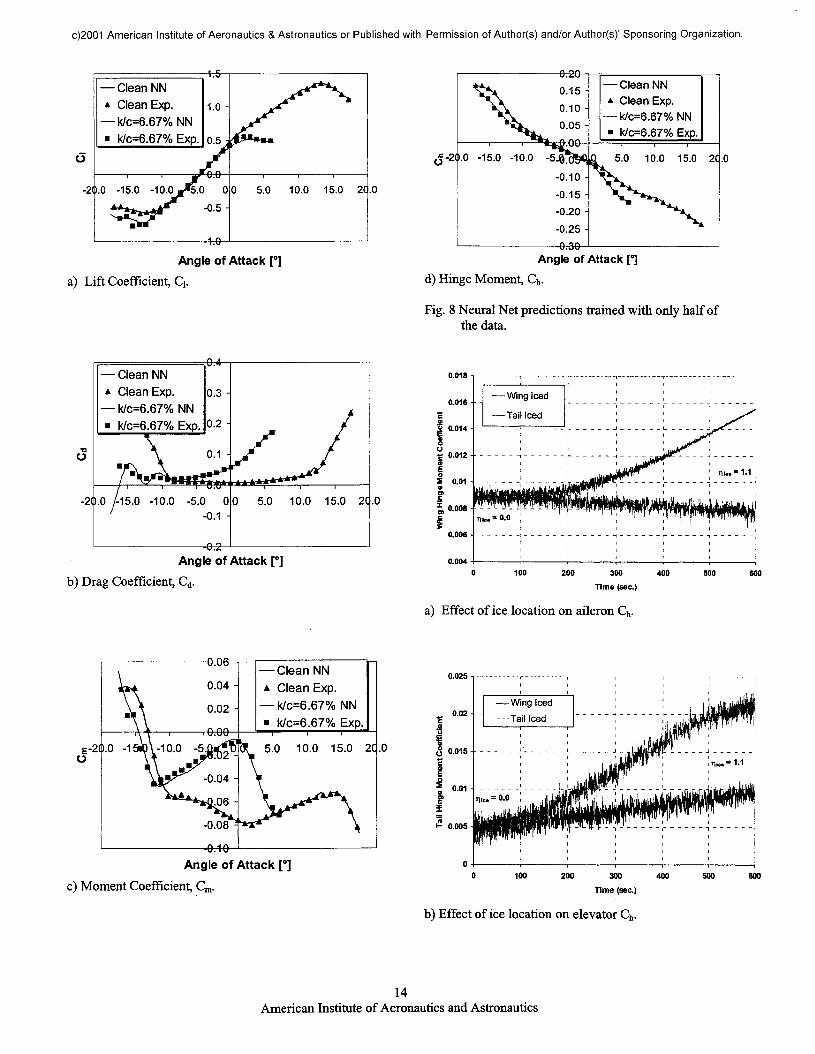
The next step was to create new neural networkstrained with only half of the available data. Every otherangle of attack point was used. In this way the neuralnet can be evaluated against data that were not in thetraining database. The results for all four aerodynamiccoefficients from the neural network trained on half ofthe available data are presented in Fig. 8. The case



shown was the same as shown in Fig. 7, with the hornlocated at an s/c of 3.4%. The configuration of thenetwork was the same as well, with five hidden layersof ten nodes each. In Fig. 7 the neural net datapresented were generated at 0.1° increments to producemany points not in the training data. As can be seenfrom the figures, training the neural network with onlyhalf of the available data had a minimal effect on thenetwork's ability to predict the aerodynamiccoefficients.

Figure 8 a) presents the predicted (denoted by NN)and experimental lift coefficients for the clean and icedcases. The predicted values of the network show agood agreement with the experimental data. Inaddition, the network also adequately captured thereduction in Qmax and ccmax.

Figure 8 b) shows the predicted and experimentaldrag coefficients for the iced and clean cases. Thecorrelation was good, with slight deviations at the morenegative angles of attack. This was understandable, asmost of the experimental data itself were ratheranomalous as the angle of attack became morenegative. At positive angles of attack, however, thenetwork was able to adequately predict the dragcoefficients.

In Fig. 8 c), the moment coefficients for both caseswere presented. Overall the correlation was more thanacceptable, and the trends were adequately captured.

Finally, Fig. 8 d) demonstrates the correlationbetween the predicted and experimental hinge-moments. Since the change in the hinge-moment datawas subtle with the accretion of ice, the network wasable to predict the values of hinge-moment with a highdegree of accuracy. More importantly, the network wasable to adequately predict the subtle changes, such asthe movement of the break point to a lower angle ofattack as the ice accretes. Comparisons were also madefor the other simulated ice shape sizes and locationswith similarly good comparison between the data andthe neural net predictions. Research is now underwayto expand this to other airfoils and simulated iceaccretions.

3.3 Trimmed Flight Characterization

The paper by Bragg et al.1 showed that the effectand onset of icing on an aircraft can be determined bycomparing iced aerodynamic performance values suchas velocity, angle of attack and elevator deflection, tothe corresponding clean values for similar flightconditions. However, the paper also illustrated thedifficulty in resolving wing icing from tail plane icing

using aerodynamic performance values - tail icingresembled a less severe wing icing case.

To distinguish between tail and wing ice, hinge-moment models for the wing and tail surfaces wereused. Figure 9 illustrates the results obtained when theaircraft accretes tail ice only, or, wing ice only, byobserving the outputs, Ch and Ch>RMS, obtained from theailerons and the elevators. Since the aileron deflectionused in the FDC code was defined for the right aileron,the aileron hinge-moment measurements were modeledonly for the aileron on the right side of the aircraft. Forall cases a constant power, constant altitude flight, wasmaintained by the autopilot feature of the FDC, with thefollowing initial trim conditions:

• Altitude of 7550 ft• Velocity of 155 knots• 77 (t = 0 s) = 0.0

The turbulence was chosen such that the aircraftexperienced RMS z-accelerations of 0.15 g. The icingcloud simulated was such that after 600 seconds the iceaccretion was represented by 77 = 0.10. (rj ice = 1.1).

An analysis of Fig. 9 a) and b) shows that wing iceonly and tail ice only can be differentiated by observingboth the aileron and elevator hinge-moments. In a wingonly ice case, the aileron Ch increased almost two-fold,but the elevator Ch remained almost constant.Similarly, in the tail only ice case, the aileron Chchanged slightly over the 600 second period, but theelevator Ch increased by almost 400%. The change inaileron Ch in the tail ice only case was primarily due tothe dependence of Ch on angle of attack, whichincreased to maintain trim during the iced flight.

Clearly, the hinge-moment measurement, C/,, canbe an important input to a method to differentiatebetween wing ice and tail ice accretion. If there was asignificant rise in the aileron hinge-moment, but littlechange in the elevator hinge-moment, it was probablydue to wing only ice. Similarly, if there was anincrease in the elevator hinge-moment, but little changein aileron hinge-moment it was probably due to tailonly ice. If both the aileron hinge-moment and theelevator hinge-moment increase, it can be inferred thatthere was ice build-up on both the wing and tailsurfaces.

The RMS hinge-moment measurements, Ch>RMS,displayed similar trends, but were not as effective indetecting ice accretion as the hinge-momentmeasurement, Ch for the continuous cruise case testedhere. This was due to the low angles of attack duringthe simulations. The ChtRMS increased only at highangles of attack where there was flow separation nearthe control surfaces. The sudden increase observed in



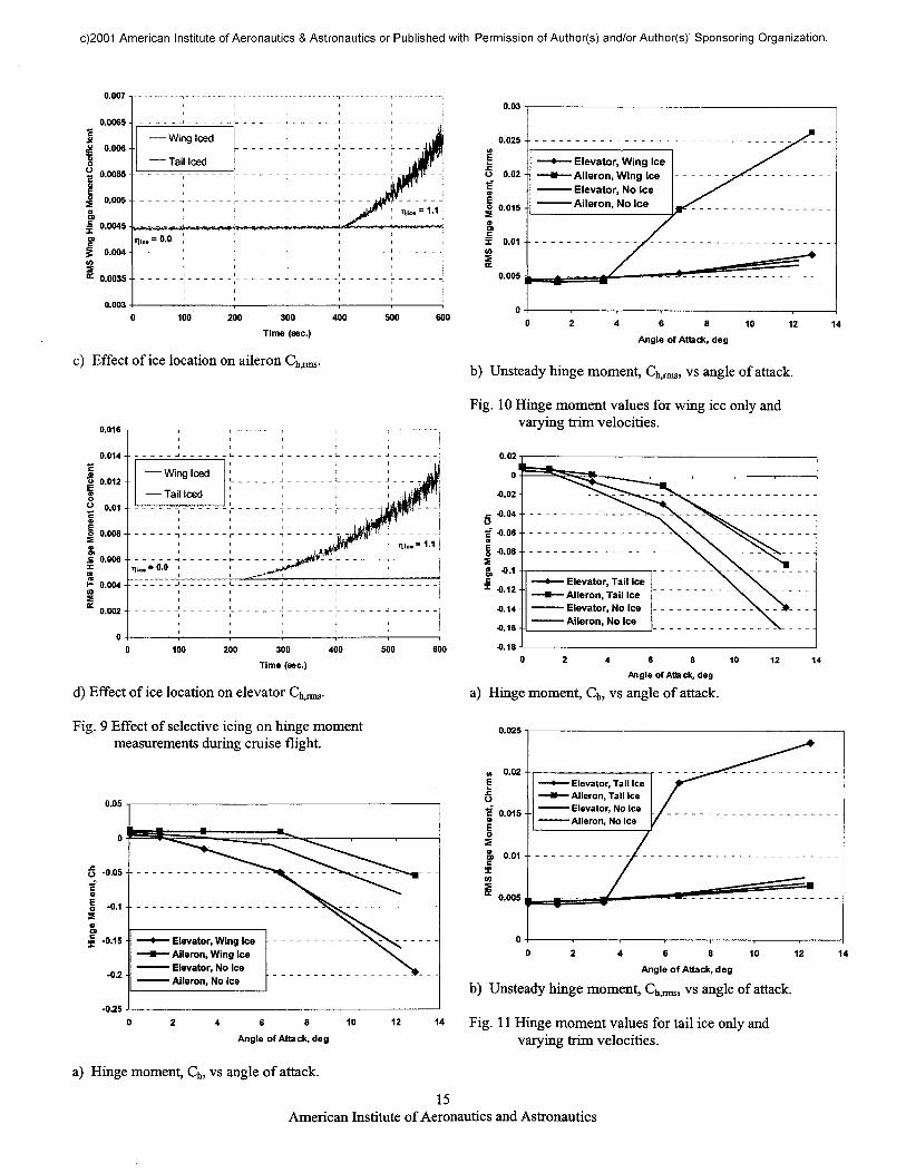
the ChiRMS was due to the nature of the Ch>RMS modelillustrated in Fig. 3. An increase in the elevatordeflection caused the break in the curve to occur at alower angle of attack, as did an increase in the icingseverity factor, 77. As Fig. 9 c) and d) show, noticeablechange in ChtRMS occured after a relatively long periodof time - more than twice the time it took to notice asimilar change in the Ch measurements.

An attempt was also made to characterize thelocation of ice using hinge-moment measurements andangle of attack at several trim velocities. Thesescenarios provided the opportunity to detect thelocation of ice over a wide spectrum of velocity valuesat a constant icing severity factor. This informationcould help in determining a suitable approach-to-landing speed for an iced aircraft, thereby avoidingstall. For all cases, a constant altitude flight maintainedby the autopilot feature of the FDC was simulated withthe following initial trim conditions:

• Altitude of 6560 ft• T]ice = 0.7

Since a constant altitude flight was chosen, as thetrim velocity decreased, the trim angle of attackincreased to maintain lift to sustain the aircraft at thespecified altitude. The elevator and aileron hinge-moment calculations and angle of attack were obtainedat the following trim velocities and resulting angles ofattack with wing ice (w_ice) and tail ice (t_ice):

• V = 78 kts ; a = 12.9° (wjce), 12.5° (t_ice)• V = 97 kts; a = 6.8° (w_ice), 6.6° (t_ice)• V = 117 kts; a = 3.4° (w_ice), 3.3° (t_ice)• V = 136 kts; a = 1.38° (wjce), 1.38° (t_ice)• V = 155 kts; a = 0.05° (wjce), 0.04° (tjce)

Figure 10 a) and b) show Ch and ChtRMSrespectively, as a function of angle of attack for theelevator and aileron in both the wing ice only and cleancase. Figure 11 a) and b) show Ch and Ch>RMSrespectively, as a function of angle of attack for theelevator and aileron in both the tail ice only and cleancase.

For the Ch variation as a function of angle of attackin the wing ice only case, as shown in Fig. 10 a), theelevator hinge-moment showed little change betweenclean and iced conditions as expected, while the aileronhinge-moment showed a modest variation between theclean and iced cases. The Ch,RMS variation as a functionof angle of attack, Fig. 10 b), showed a drastic increasein the RMS aileron hinge-moment. For the iced case,the Ch>RMS rose from 0.005 at an angle of attack of 3.5°to 0.015 at an angle of attack of 7°, and to 0.027 at anangle of attack of 12.5°. There was little change in the

aileron Ch>RMS value for the clean case as the airfoil didnot approach stall at angles of attack less than 12 °. Asexpected, the elevator Ch>RMS showed little change forthe wing only iced case.

Similarly, the tail ice only case, Fig. 11, showedthe RMS hinge-moment value provided a quickerindication of ice accretion on the tail surface. For theiced case, the Ch>RMS rose from 0.005 at an angle ofattack of 3.5° to 0.018 at an angle of attack of 6.5°.This jump in values of Ch>RMS while comparing theclean condition to the iced condition provided a clearand early indication of the location of ice at angles ofattack within the safe flight envelope. The hinge-moment values, C/,, provided reasonable data at lowangles of attack and the RMS hinge-moment values,Ch,RMs* provide excellent warnings of ice build-up athigher angles of attack. The unsteady hinge-momentsensor measurements, ChtRMs> provided a good warningof eminent stall and its applicability as an envelopeprotection tool should be explored.

3.4 Atmospheric DisturbanceAnalysis

In order to compare the effect of microbursts andicing on aircraft performance, flight through 11different microbursts were simulated using the FDC.The intensity of the microbursts were varied bysystematically varying the radius and umax, themaximum outflow of the microburst. For allsimulations the aircraft was at 136 kts, and altitudesfrom 1312 ft to 2625 ft. An altitude hold autopilotsetting with no recovery maneuver was used duringeach microburst simulation in FDC. No recoverymaneuver was performed because these simulationswere performed under the assumption that themicroburst could be mistaken for icing and performinga recovery maneuver indicates that the microburst hadbeen identified. The microburst parameters have beenprovided in Table 2. Sample wind velocities formicroburst #5 have also been provided in Fig. 12.

It was determined that the pitch rate due to windgust term, qg term, had little effect on the microburstresults. Fig. 13 is an example of the differencesbetween the angle of attack response of the aircraft withand without the qg term. It can be seen that the resultswere virtually identical.

The aircraft response to two microburst encounterswere compared to three icing encounters and reportedin Fig. 14. Angle of attack, velocity, altitude, andelevator angle vs. time can be seen for microbursts #5and #9 and icing conditions rjice = 0.50, r|ice = 0.91, andT]ice = 1.10 Figs. 14 a) - d), respectively. All fourfigures show that the changes in angle of attack,



velocity, altitude, and elevator angle due to icing werevery gradual and the changes due to the microburstswere much more rapid and pronounced. In the altitudecase, the autopilot was able to maintain altitude duringthe icing cases while it was not able to maintain altitudeduring the microbursts. Table 3 summarizes themaximum rates of change for angle of attack, velocity,altitude, and elevator angle for six microbursts andthree icing cases. Many of the microburst rates ofchange were an order of magnitude larger than the icingcases. The rates of change of icing that are similaroccur well beyond the time it would take to go througha microburst. By monitoring the rates of change andthe altitude it should be possible to distinguish betweenicing and microbursts. This could be accomplishedusing a neural net where the change with time can beincorporated.21

In addition to mircrobursts, gravity waves couldpotentially pose a challenge in aircraft ice detectionusing the SIS. A simple sine wave was used toapproximate the downdraft velocity of the gravitywaves in the FDC code. The amplitudes andwavelengths of these waves were varied from 0.486 kts.(1 m/s) to 7.7754 kts. (4 m/s) and 1 mile to 15 milesrespectively.18'22 The periods of these wave encounterswere set by the aircraft airspeed of 136 kts. Table 4 hasbeen included specifying parameters of the gravitywaves analyzed.

The resulting angle of attack, velocity, elevatordeflection, altitude, and hinge-moment graphs for theicing and microburst encounters have been included inFigs. 15 a) - f), respectively. In the first 100 secondsthe results for icing and the gravity wave cases weresimilar. This was especially true for the smallamplitude and large wavelength waves. The icingsimulations shown were for a constant power setting,therefore, as discussed earlier, ice accretion increaseddrag which caused a reduction in airspeed. As a resultof the increase in drag and reduction in airspeed theaircraft increased angle of attack to maintain altitude.Similarly, with the gravity waves, the downdraft forcedthe aircraft to increase angle of attack to maintainconstant altitude. This change in angle of attack causedthe aircraft to reduce velocity and make otherassociated trim changes. Although the mechanisms ofboth these phenomenon were different, the performanceand handling qualities effects were very similar.However, icing also affects the aerodynamics of theaircraft in other ways not duplicated by gravity waves.These include reduction in control power, lift-curveslope, static margin, etc. Exploring these effects shouldprovide avenues to distinguish ice accretion.

Considering the results of the gravity waveanalysis, a much more in depth study may be

warranted. The sine wave used to approximate thedowndraft is simplistic. This must be refined to modelmore of the diversity of the phenomenon. Themechanisms that cause the changes in aircraftperformance and handling qualities need to be studiedin more detail. This analysis will identify thedifferences in such a way that algorithms can bedeveloped to provide good identification. The NeuralNetwork methods used to identify icing can be trainedbased on these characteristics.

4.0 CONCLUSIONS

A method to study the effect of ice accretion on theflight dynamics of an aircraft has been developed. Themethod was used to evaluate a method for sensing iceaccretion through the change in steady-state aircraftparameters. Conclusions from this study include:

1. The neural net did a good job of fitting theaerodynamic coefficients for the clean and icedairfoil data. This holds promise as a method toreplace the r|ice method currently in use to modelthe effect of ice on aircraft parameters.

2. The use of control surface hinge-moment modelingprovided a potentially useful tool in determiningthe location of ice accretion.

3. The unsteady hinge-moment predictions providedexcellent information at high angle of attack whichsuggests their use for envelope protection.

4. The clean aircraft in a microburst experiencesperformance and control changes significantlydifferent in character from an icing encounter.

5. The simple gravity wave models used in this paperproduced aircraft performance and control changessimilar to the drag increase-induced changes of anicing encounter. This warrants closer examinationto ensure that it can be distinguished from an icingencounter using iced-aircraft characteristics notrelated to the drag rise.

Research is currently underway to improve the icedaircraft models used in this paper, to examine moreclosely gravity waves and other atmosphericphenomena so that they can be distinguished from icingeffects, and to develop real-time envelope protectionmethods for iced aircraft.

5.0 ACKNOWLEDGEMENTS

This work was supported in part by NASA Glenn grantNAG 3-21235. The authors would like to thank Mr.Tom Bond, Mr. Tom Ratvasky and Dr. Mark Potapczuk



of NASA Glenn for their contributions. This work wasalso supported by a Critical Research Initiatives grantfrom the University of Illinois at Urbana-Champaign.Several members of the Smart Icing Systems researchgroup at Illinois contributed to this research including,Prof. Tamer Basar, Mr. Jim Melody, Prof. NadineSarter, Mr. Sam Lee and many others. The authorswould also like to thank Dr. Marcia Politovich ofNCAR for her tutelage on microbursts and gravitywaves.

REFERENCES

1 Bragg, M.B., Hutchison, T., Merret, J., Oltman, R.,and Pokhariyal, D., "Effects of Ice Accretion onAircraft Flight Dynamics," AIAA Paper No. 2000-0360, Reno, NV, Jan. 2000.

2 Bragg, M.B., "Aircraft Aerodynamic Effects Due ToLarge-Droplet Ice Accretions," AIAA Paper No. 96-0932, Reno, NV, Jan. 1996.

3 Shaw, Robert J., Ray G. Sotos, and Frank R. Solano,"An Experimental Study of Airfoil IcingCharacteristics," NASA TM 82790, Jan. 1982.

4 Shin, Jaiwon, and Thomas H. Bond, "Results of anIcing Test n a NACA 0012 Airfoil in the NASALewis Icing Research Tunnel," NASA TM 105374,Jan. 1992.

5 Olsen, William, Robert Shaw, and James Newton,"Ice Shapes and the Resulting Drag Increase for aNACA 0012 Airfoil," NASA TM 83556, Jan. 1984.

6 Haykin, Simon, "Neural Networks: A ComprehensiveFoundation," Prentice Hall, Inc., Upper Saddle River,New Jersey, 1999.

7 Kirn, H.S., and Bragg, M.B., "Effects of Leading-Edge Ice Accretion Geometry on AirfoilAerodynamics," 17th AIAA Applied AerodynamicsConference, Norfolk, VA, June 1999.

8 Ranaudo, R.J., Batterson, J.G., Reehorst, A.L., Bond,T.H. and O'Mara, T.M., "Determination ofLongitudinal Aerodynaimc Derivatives Using FlightData From an Icing Research Aircraft," NASA TM101427 and AIAA 89-0754, Jan. 1989.

9 Ratvasky, T.P. and Ranaudo, R.J., "Icing Effects onAircraft Stability and Control Determined fromFlight Data," NASA TM 105977 and AIAA 93-0398,Jan. 1993.

10 R.J. Ranuado, et.al., "The Measurement of AircraftPerformance and Stability and Control After FlightThrough Natural Icing Conditions," AIAA 86-9758,1986.

11 Rauw, Marc, "FDC 1.3 - A SIMULINK Toolbox forFlight Dynamics and Control Analysis," 1998.

12 Miller, R and Ribbens, W., "The Effects of Icing onthe Longitudinal Dynamics of an Icing ResearchAircraft," AIAA Paper No. 99-0636, Reno, NV, Jan.1999.

13 Ratvasky, T.P., Van Zante, J.F., and Riley, J.T.,"NASA/FAA Tailplane Icing Program Overview,"AIAA Paper No. 99-0370, Reno, NV, Jan. 1999.

14 Gurbacki, H.M., and Bragg, M.B., " Sensing AircraftIcing Effects by lap Hinge Moment Measurements",17th AIAA Applied Aerodynamics Conference,Norfolk, VA, June 1999.

15 Pokhariyal, D., "Effect of Ice Accretion on AircraftPerformance and Control During Trimmed Flight,"M.S. Thesis, University of Illinois, Urbana, IL, Dec.2000.

16 Mulgund, S.S., and Stengel, R.F., "Target PitchAngle for the Microburst Escape Maneuver," Journalof Aircraft, Vol. 30, No. 6, Nov.-Dec. 1993.

17 Oseguera, R.M., and Bowles, R.L., "A simpleAnalytical 3-Dimensional Downburst Model Basedon Boundary Layer Stagnation Flow," NASA TM1000632.

18 Sica, R.J., "A Short Primer on Gravity Waves," 1999.http://pcl.physics.uwo.ca/pclhtml/gravitywaves.html.

19 Etkin B., and Etkin D., "Critical Aspects ofTrajectory Prediction: Flight in Non-uniform Wind,"AGARDograph No. 301, V. 1, 1990.

20 Bruun, H. H., "Hot-Wire Anemometry: Principlesand Signal Analysis," Oxford, New York 1995.

21 Melody, J., Pokhariyal, D., Merret, J., Basar, T.,Perkins, W., and Bragg, M., "Sensor Integration forInflight Icing Characterization Using NeuralNetworks," AIAA paper No. 2001-0542, Jan. 2001.

22 Politovich, Marcia, Private Communication,December 12, 2000.

10American Institute of Aeronautics and Astronautics


Table 1 Non-dimensional Derivatives for Twin Otter in Clean and Iced Confij

cleanwingjcetail iceall iced

Czo-0.380-0.380-0.380-0.380

Cza

-5.660-5.342-5.520-5.094

Czq-19.970-19.700-19.700-19.700

Cz6e-0.608-0.594-0.565-0.550

GXO-0.041-0.050-0.046-0.062

K0.0520.0530.0530.057

Cmo0.0080.0080.0080.008

Cma

-1.310-1.285-1.263-1.180

mrations.Cmq

-34.200-33.000-33.000-33.000

C,**-1.740-1.709-1.593-1.566

cleanall iced

CYp-0.6

-0.48

CYP

-0.2-0.2

CYr

0.40.4

CY8r0.150.138

c,p-0.08-0.072

c.P-0.5

-0.45

C,r

0.060.06

C,sa

-0.15-0.135

CBr

0.0150.0138

Cnp

0.10.08

Cnp

-0.06-0.06

Cnr

-0.18-0.169

Cnsr

-0.12-0.11

Cns.

-0.001-0.001

Table 2 Microburst Analysis Parameters.Microburst Number

1234567891011

Microburst ParamatersR(ft)10001000100030003000300030003000500050005000

Umax (ft/s)510205102060120102040

Zmax (ft)150150150150150150150150150150150

SeverityUmax/R(l/s)

0.00500.01000.02000.00170.00330.00670.02000.04000.00200.00400.0080

Table 3 Rate of Change Comparison for Icin > and Microbursts.Case

Microburst 1Microburst 2Microburst 4Microburst 5Microburst 6Microburst 9

riice= 0.50, Ti/r|ice= 0.08Tlicc= 0.9 l,Tl/T|ice= 0.09

r,ice= 1.10, ri/r,ice= 0.09

dcx/dt (deg/s)0.17180.38300.02690.04720.13450.02290.00400.02040.1030

dV/dt (kts/s)-0.4505-1.1468-0.2000-0.6000-1.5000-0.2917-0.0323-0.7951-0.2537

dh/dt (ft/min)-466.6-990.3-150.0-150.0-266.7-55.50.00.0-5.0

d5e/dt (deg/s)-0.0343-0.0805-0.0143-0.0427-0.0851-0.02030.0039-0.0196-0.0943

Table 4 Gravity Wave Parameters.

Wavelengthmiles

151015

meters160080001600024000

Downdraft Velocity (kts)0.000 0.486 1.944 7.775

Period at an airspeed of 136 kts (sec)22.86114.29228.57342.86

22.86114.29228.57342.86

22.86114.29228.57342.86

22.86114.29228.57342.86



Hidden Layers

Fig. 1 Schematic of Neural Network.

CuVs.a as a function of 6c and TIn t

0.06

-0.06

-0.12

-0.18

OutputLayer

-10

a) Ch model showing variation with a, 8E and rj.

155 10

Alpha, deg

a) Ch,RMs model showing variation with a, 8E and rj.

20

0 5

Alpha, deg

b) Experimental ChiRMS data for NACA 23012 airfoil.

Fig. 3 Unsteady hinge RMS, ChtRMS, model compared toexperimental data.

Alpha, deg

b) Experimental Ch data for NACA 23012 airfoil.

Fig. 2 Hinge moment, Ch, model compared toexperimental data.

Fig. 4 Microburst Encounter Diagram. 17



7.0

6.0

5.0

|4.0

1,0

1"|o 1.0<

0.0

-1.0

-2.0

—FDQPtesent Method—Journal of Aircraft

-10000 -8000 -6000 -4000 -2000 0 2000 4000Position (ft)

13

6000 8000 10000

Fig. 5 Verification trajectories.

-B-Static T=08F-»- Static T=10°F-•- Static T=20°F-A-Static T=25°F-*-Static T=29°F

5.0 10.0 20.0 25.0MVD (microns)

30.0 35.0

c) Effect of MVD on TJ

Fig. 6 Effect of cloud properties on the aircraft icingparameter r|.

0.50 1.00LWC (g/m3)

1.50 2.00

a) Effect of LWC on TJ.

- Clean NNClean Exp.

-k/c=6.67% NN

k/c=6.67% Exp.

a) Lift Coefficient, Q.Angle of Attack [°]

-10.0 0.0 5.0 10.0 15.0Static T (°F)

20.0 25.0 30.0

b) Effect of static temperature on TJ.

— Clean NN

Clean Exp.

k/c=6.67% NN

k/c=6.67% Exp.

10.0 15.0 20.0-20.0 -15.0 -10.0 -5.0 0.0 5.0

Angle of Attack [°]

b) Drag Coefficient, Cd.

Fig. 7 Neural net predictions, trained with all data.



— Clean NNA Clean Exp.

— k/c=6.67%NN— k/c=6.67% Exp.

o

Angle of Attack [°]a) Lift Coefficient, Q.

o

0.15-

0.10 -

0.05 -

-20.0 -15.0 -10.0

-0.30


— k/c=6.67%NN— k/c=6.67% Exp.

5.0 10.0 15.0 2C

Angle of Attack [°]d) Hinge Moment, Ch.

Fig. 8 Neural Net predictions trained with only half ofthe data.


— k/c=6.67%NNk/c=6.67% Exp.

0.3

0.2

10 /-15.0 -10.0 -5.0-0.1

5.0 10.0 15.0 2C.0

Angle of Attack [°]b) Drag Coefficient, Cd.

E-20.0 -1

— Clean NNClean Exp.k/c=6.67% NNk/c=6.67% Exp.

Angle of Attack [°]c) Moment Coefficient, Cm.

0.018

100 200 300 400

Time (sec.)

a) Effect of ice location on aileron Ch.

0.025 -i

100 200 300 400 500

b) Effect of ice location on elevator Ch.



0.03

200 300 400

Time (sec.)500 600

c) Effect of ice location on aileron Ch,rms.

0.016

200 300 400

Time (sec.)500 600

d) Effect of ice location on elevator

Fig. 9 Effect of selective icing on hinge momentmeasurements during cruise flight.

0.05

Elevator, Wing IceAileron, Wing IceElevator, No IceAileron, No Ice

0.025

O 0.02

o

o 0.015 -

X 0.01CO

0.005

- Elevator, Wing Ice-Aileron,Wing Ice- Elevator, No Ice- Aileron, No Ice

4 6 8 10

Angle of Attack, deg12 14

b) Unsteady hinge moment, Ch>rms, vs angle of attack.

Fig. 10 Hinge moment values for wing ice only andvarying trim velocities.

Elevator, Tail IceAileron, Tail IceElevator, No IceAileron, No Ice

0 2 4 6 8 10Angle of Attack, deg

a) Hinge moment, Ch, vs angle of attack.

0.025

w 0.02EjEoc" 0.015

0.01 -

0.005

- Elevator, Tail Ice-Aileron, Tall Ice- Elevator, No Ice-Aileron, No Ice

-025

0 2 4 6 8 1 0Angle of Attack, deg

b) Unsteady hinge moment, C^tTmS) vs angle of attack.

4 e s 10 12 14 Fig. 11 Hinge moment values for tail ice only andAngle of Attack, deg varying trim velocities.

12 14

a) Hinge moment, Ch, vs angle of attack.



5.0

4.0

I30

|2.0

> 1.0|£ 0.0

-1.0

0

12 S,

: r ............. uw,WindX-Component": ,\ —————— Vw,WindY-Component'- — — • Ww,WindZ-Component: f 1 1 —————————————————— 1

': 1 j

- / 1

; x/

0 100.0 200.0 300.0 400.0Time (sec)

ample wind velocities for microburst #5.

140.0

130.0

^ 120.0

1| 110'°> 100.0

90.0

80.0o

;

-

^^rr:............. Microburst #5—————— Microburst #9

—— —— • ^1 = 0.91,71/11^ = 0.09

X. \"\%\\\

0 100.0 200.0 300.0 400.0Time (sec)

b) Velocity for microbursts and icing.

Microburst #5 without qg TermMicroburst #5 with qg Term

100.0 200.0 300.0 400.0Time (sec)

Fig. 13 qg Effect on the microburst encounter.

1700

1675

1650

1625

1600

1575

1550

1525

15000 0 100.0

-

'•

————— Microburst#9

—— —— - Tiice = 0.91,Ti/Tlice=:0-09

200.0 300.0 400.0

7600

7500

7400g

7300 |

<37200

7100

7000

Time (sec)

c) Altitude for microbursts and icing.

14.0

12.0

|10.0

'I8'0

^6.0

|4.0

2.0

0.0

:

:

............. Microburst #5

—— —— • ilice = 0.91, r|/Tjice = 0.09

^^''^^- "~~

-~"^^>^Lr~

!/

/' .s

0.0 100.0 200.0 300.0Time (sec)

a) Angle of attack for microbursts and icing.

400.0

2.0

0.0

!,,.2

|-4.0Q

1 -6.0

S-8.0

-iou0 0

~^^-^^^- - -

——— ——— • /nice==0-91»Tl/Tlice = 0-09

—— -- —— --- 11^=1.10,11/11^ = 0.09

i i i

100.0 200.0 300.0

- • — . — _ _ _^^-*-\ ^^x^

X\\

\,

400.0Time (sec)

d) 5e for microbursts and icing.

Fig. 14 Comparison of the effects of micobursts andicing on aircraft parameters.



lO.Oq

9.0

8.0

a 7.0

Icing; r}^- 0.50, TI/TI, = 0.08Icing; 1]^ = 0.91, i}/^ = 0.09Icing; = 1.10, TI = 0.09G. Wave; Ww = 0.25 Period = 342.86G. Wave; Ww = 1.00 Period = 342.86G. Wave; Ww = 0.25 Period = 228.57G. Wave; Ww = 1.00 Period = 228.57

100.0 200.0 300.0Time (sec)

400.0

7600 q

7590 i

7580^

7570^

g 7560^<o :

*O 7^<fi 2

% 7*540 -^ / J*tU .

7530 i

7520 \

'Tcnfi '75004

— .... — . — ........ icing, TJ — 0.91, TJ/T|. — 0.09Icing; TI = 1 .1 0, TI/TI = 0.09

- - - - G. Wave; Ww = 0.25 Period = 342.86_ _ _ _ G. Wave; Ww = 1 .00 Period = 342.86

G. Wave; Ww = 0.25 Period = 228.57— -- — G. Wave; Ww = 1.00 Period = 228.57

i

/ ,A^'~^s | /j*^ _^~s- - -~ '?~ ~ — - - x \ ?' • "\ •"*" **m*-y™-^ •*" """"•»""------ •••-• .""""-.; __ ^ _.. ... ^rf™..«l»..Jt.ttnj.

^.:/- |\ / p-^-^

^ ... .. .... . _....„_.....„...„.. ...

O' 100.6 ' ' 200.6 ' ' 300.6Time (sec)

1

,-.-.-ll.. r

i1

400.0

a) Angle of attack for icing and gravity waves. d) Altitude for icing and gravity waves.

100.090.0

80.0

70.0

Icing; n " 0.50, T^ • 0.08Icing; TI ta * 0.91, TI/TJ^ = 0.09Icing; r\ » 1.10, TI/TJ^ * 0.09G. Wave; Ww = 0.25 Period * 342.86G. Wave; Ww = 1.00 Period = 342.86G. Wave; Ww = 0.25 Period * 228.57G. Wave; Ww * 1.00 Period * 228.57

0.0 100.0 200.0 300.0Time (sec)

400.0

b) Velocity for icing and gravity waves.

0.0050:

0.0049 \

0.0048^

0.0047 [

•J 0.0046^

10.0045 \

0.0044:0.0043 i - -——0.0042 f0.0041 \-0.0040

--_]_.-'><• ~ _._! . ._.-• ' ' ' * h-—1-1-

Icing; i\^ = 0.50, TI/TI = 0.08Icing; TI „, = 0.91, H/T^ = 0.09Icing; r\ ^ = 1.10, TJ/TJ, = 0.09G. Wave; Ww = 0.25 Period = 342.86G. Wave; Ww = 1.00 Period = 342.86G. Wave; Ww = 0.25 Period = 228.57G. Wave; Ww = 1.00 Period = 228.57

00 100.0 200.0 300.0Time (sec)

400.0

e) RMS elevator hinge moment coefficient for icing andgravity waves.

0.0:

&o -8.0

| -10.0:

-12.0

-14.0

Icing; TI to = 0.50, TI/TI = 0.08Icing; TI ta = 0.91, TI/TI = 0.09Icing; TI = 1.10, i\li\^ - 0.09G. Wave; Ww = 0.25 Period = 342.86G. Wave; Ww = 1.00 Period = 342.86G. Wave; Ww = 0.25 Period = 228.57G. Wave; Ww = 1.00 Period = 228.57

0.0 100.0 200.0 300.0Time (sec)

400.0

c) Elevator deflection for icing and gravity waves.

0.000

u-0.050-

————— Icing; TI = 0.50, TI/TI = 0.08————— Icing; j\ = 0.91, TJ/T]^ = 0.09

Icing; TI = 1.10, TI/TJ, = 0.09~ - - - G. Wave; Ww = 0.25 Period = 342.86— - - - G. Wave; Ww = 1.00 Period = 342.86

G. Wave; Ww = 0.25 Period = 228.57—--— G. Wave;Ww = 1.00 Period = 228.57

00 100.0 200.0 300.0Time (sec)

400.0

f) Elevator hinge moment coefficient for icing andgravity waves.

Fig. 15 Comparison of the effects of gravity waves andicing on aircraft parameters.


aircraft flight dynamics with simulated ice...

Documents