Aircraft Control ToolboxUser’s Guide

This software described in this document is furnished under a license agreement. The software may be used, copied or translatedinto other languages only under the terms of the license agreement.

Aircraft Control Toolbox

Compiled on: June 26, 2017

c©Copyright 2004-2006, 2017 by Princeton Satellite Systems, Inc. All rights reserved.

MATLAB is a trademark of the MathWorks.

All other brand or product names are trademarks or registered trademarks of their respective companies or organizations.

Printing History:

December 15, 2005 First Printing v1.0July 15, 2006 Second Printing v1.1 August 16, 2012 v4.0July 11, 2014 v2016.1June 26, 2017 v2017.1

Princeton Satellite Systems, Inc.6 Market St. Suite 926Plainsboro, New Jersey 08536

Technical Support/Sales/Info: http://www.psatellite.com

ii

CONTENTS

1 Introduction 11.1 Organization . . . . . . . . . . . . . . . . . . . . . . . . . . . . . . . . . . . . . . . . . . . . . . . . 11.2 Requirements . . . . . . . . . . . . . . . . . . . . . . . . . . . . . . . . . . . . . . . . . . . . . . . 21.3 Installation . . . . . . . . . . . . . . . . . . . . . . . . . . . . . . . . . . . . . . . . . . . . . . . . 21.4 Getting Started . . . . . . . . . . . . . . . . . . . . . . . . . . . . . . . . . . . . . . . . . . . . . . 2

2 Fundamentals 52.1 Aircraft Properties Database . . . . . . . . . . . . . . . . . . . . . . . . . . . . . . . . . . . . . . . 52.2 Classes . . . . . . . . . . . . . . . . . . . . . . . . . . . . . . . . . . . . . . . . . . . . . . . . . . 6

2.2.1 Class: acstate . . . . . . . . . . . . . . . . . . . . . . . . . . . . . . . . . . . . . . . . . 62.2.2 Class: statespace . . . . . . . . . . . . . . . . . . . . . . . . . . . . . . . . . . . . . . 7

2.3 Code Conventions . . . . . . . . . . . . . . . . . . . . . . . . . . . . . . . . . . . . . . . . . . . . . 9

3 Getting Help 113.1 MATLAB’s Built-in Help System . . . . . . . . . . . . . . . . . . . . . . . . . . . . . . . . . . . . 11

3.1.1 Basic Information and Function Help . . . . . . . . . . . . . . . . . . . . . . . . . . . . . . 113.1.2 Published Demos . . . . . . . . . . . . . . . . . . . . . . . . . . . . . . . . . . . . . . . . . 12

3.2 MATLAB Help . . . . . . . . . . . . . . . . . . . . . . . . . . . . . . . . . . . . . . . . . . . . . . 123.3 FileHelp . . . . . . . . . . . . . . . . . . . . . . . . . . . . . . . . . . . . . . . . . . . . . . . . . . 15

3.3.1 Introduction . . . . . . . . . . . . . . . . . . . . . . . . . . . . . . . . . . . . . . . . . . . . 153.3.2 The List Pane . . . . . . . . . . . . . . . . . . . . . . . . . . . . . . . . . . . . . . . . . . . 163.3.3 Edit Button . . . . . . . . . . . . . . . . . . . . . . . . . . . . . . . . . . . . . . . . . . . . 163.3.4 The Example Pane . . . . . . . . . . . . . . . . . . . . . . . . . . . . . . . . . . . . . . . . 163.3.5 Run Example Button . . . . . . . . . . . . . . . . . . . . . . . . . . . . . . . . . . . . . . . 163.3.6 Save Example Button . . . . . . . . . . . . . . . . . . . . . . . . . . . . . . . . . . . . . . . 163.3.7 Help Button . . . . . . . . . . . . . . . . . . . . . . . . . . . . . . . . . . . . . . . . . . . . 163.3.8 Quit . . . . . . . . . . . . . . . . . . . . . . . . . . . . . . . . . . . . . . . . . . . . . . . . 16

3.4 Searching in File Help . . . . . . . . . . . . . . . . . . . . . . . . . . . . . . . . . . . . . . . . . . 173.4.1 Search File Names Button . . . . . . . . . . . . . . . . . . . . . . . . . . . . . . . . . . . . 173.4.2 Find All Button . . . . . . . . . . . . . . . . . . . . . . . . . . . . . . . . . . . . . . . . . . 173.4.3 Search Headers Button . . . . . . . . . . . . . . . . . . . . . . . . . . . . . . . . . . . . . . 173.4.4 Search String Edit Box . . . . . . . . . . . . . . . . . . . . . . . . . . . . . . . . . . . . . . 17

3.5 DemoPSS . . . . . . . . . . . . . . . . . . . . . . . . . . . . . . . . . . . . . . . . . . . . . . . . . 173.6 Graphical User Interface Help . . . . . . . . . . . . . . . . . . . . . . . . . . . . . . . . . . . . . . 173.7 Technical Support . . . . . . . . . . . . . . . . . . . . . . . . . . . . . . . . . . . . . . . . . . . . . 18

4 Coordinates 214.1 Coordinate Frames . . . . . . . . . . . . . . . . . . . . . . . . . . . . . . . . . . . . . . . . . . . . 214.2 Transformation Matrices . . . . . . . . . . . . . . . . . . . . . . . . . . . . . . . . . . . . . . . . . 224.3 Quaternions . . . . . . . . . . . . . . . . . . . . . . . . . . . . . . . . . . . . . . . . . . . . . . . . 224.4 Transformation Functions . . . . . . . . . . . . . . . . . . . . . . . . . . . . . . . . . . . . . . . . . 23

iii

CONTENTS CONTENTS

5 Environment 255.1 Atmospheric Properties . . . . . . . . . . . . . . . . . . . . . . . . . . . . . . . . . . . . . . . . . . 255.2 Wind Models . . . . . . . . . . . . . . . . . . . . . . . . . . . . . . . . . . . . . . . . . . . . . . . 26

6 Simulation 296.1 Aircraft Simulations . . . . . . . . . . . . . . . . . . . . . . . . . . . . . . . . . . . . . . . . . . . . 29

6.1.1 Introduction . . . . . . . . . . . . . . . . . . . . . . . . . . . . . . . . . . . . . . . . . . . . 296.1.2 Aspects of Simulation Models . . . . . . . . . . . . . . . . . . . . . . . . . . . . . . . . . . 296.1.3 Simulating Linear Systems . . . . . . . . . . . . . . . . . . . . . . . . . . . . . . . . . . . . 306.1.4 Simulating Non-Linear Systems . . . . . . . . . . . . . . . . . . . . . . . . . . . . . . . . . 32

6.2 Creating an Interactive Simulation . . . . . . . . . . . . . . . . . . . . . . . . . . . . . . . . . . . . 336.3 Customizing a Simulation . . . . . . . . . . . . . . . . . . . . . . . . . . . . . . . . . . . . . . . . . 376.4 Simulation Graphics . . . . . . . . . . . . . . . . . . . . . . . . . . . . . . . . . . . . . . . . . . . 38

6.4.1 Simulation GUI’s . . . . . . . . . . . . . . . . . . . . . . . . . . . . . . . . . . . . . . . . . 386.4.2 Post-Simulation Plotting . . . . . . . . . . . . . . . . . . . . . . . . . . . . . . . . . . . . . 39

7 Designing Controllers 417.1 Using the block diagram . . . . . . . . . . . . . . . . . . . . . . . . . . . . . . . . . . . . . . . . . 417.2 Linear Quadratic Control . . . . . . . . . . . . . . . . . . . . . . . . . . . . . . . . . . . . . . . . . 427.3 Single-Input-Single-Output . . . . . . . . . . . . . . . . . . . . . . . . . . . . . . . . . . . . . . . . 427.4 Eigenstructure Assignment . . . . . . . . . . . . . . . . . . . . . . . . . . . . . . . . . . . . . . . . 46

8 Implementing Controllers 498.1 A General Interface . . . . . . . . . . . . . . . . . . . . . . . . . . . . . . . . . . . . . . . . . . . . 498.2 Closed-Loop Control . . . . . . . . . . . . . . . . . . . . . . . . . . . . . . . . . . . . . . . . . . . 51

8.2.1 Introduction . . . . . . . . . . . . . . . . . . . . . . . . . . . . . . . . . . . . . . . . . . . . 518.2.2 Sensor Input . . . . . . . . . . . . . . . . . . . . . . . . . . . . . . . . . . . . . . . . . . . 518.2.3 Actuator Model . . . . . . . . . . . . . . . . . . . . . . . . . . . . . . . . . . . . . . . . . . 518.2.4 Control Law . . . . . . . . . . . . . . . . . . . . . . . . . . . . . . . . . . . . . . . . . . . 52

8.3 Pilot Input . . . . . . . . . . . . . . . . . . . . . . . . . . . . . . . . . . . . . . . . . . . . . . . . . 568.4 Control Implementation . . . . . . . . . . . . . . . . . . . . . . . . . . . . . . . . . . . . . . . . . . 56

9 Performance Analysis 599.1 Concorde Properties . . . . . . . . . . . . . . . . . . . . . . . . . . . . . . . . . . . . . . . . . . . . 599.2 Breguet Range Equation . . . . . . . . . . . . . . . . . . . . . . . . . . . . . . . . . . . . . . . . . 609.3 Rate of Climb . . . . . . . . . . . . . . . . . . . . . . . . . . . . . . . . . . . . . . . . . . . . . . . 619.4 Takeoff . . . . . . . . . . . . . . . . . . . . . . . . . . . . . . . . . . . . . . . . . . . . . . . . . . 619.5 Stall Velocity . . . . . . . . . . . . . . . . . . . . . . . . . . . . . . . . . . . . . . . . . . . . . . . 62

10 Gas Turbines 6310.1 Using the Jet Engine Functions . . . . . . . . . . . . . . . . . . . . . . . . . . . . . . . . . . . . . . 6310.2 Using JetEngineDefinitions . . . . . . . . . . . . . . . . . . . . . . . . . . . . . . . . . . . . . . . . 6410.3 Using JetEngineAnalysis . . . . . . . . . . . . . . . . . . . . . . . . . . . . . . . . . . . . . . . . . 6410.4 Using JetEnginePerformance . . . . . . . . . . . . . . . . . . . . . . . . . . . . . . . . . . . . . . . 65

11 Airships 6711.1 Modeling . . . . . . . . . . . . . . . . . . . . . . . . . . . . . . . . . . . . . . . . . . . . . . . . . 67

11.1.1 Baseline Airship Design . . . . . . . . . . . . . . . . . . . . . . . . . . . . . . . . . . . . . 7011.2 Control . . . . . . . . . . . . . . . . . . . . . . . . . . . . . . . . . . . . . . . . . . . . . . . . . . 7311.3 Analysis . . . . . . . . . . . . . . . . . . . . . . . . . . . . . . . . . . . . . . . . . . . . . . . . . . 7411.4 Simulation . . . . . . . . . . . . . . . . . . . . . . . . . . . . . . . . . . . . . . . . . . . . . . . . . 74

iv

CONTENTS CONTENTS

A Using Databases 77A.1 The Constant Database . . . . . . . . . . . . . . . . . . . . . . . . . . . . . . . . . . . . . . . . . . 77A.2 Merging Constant Databases . . . . . . . . . . . . . . . . . . . . . . . . . . . . . . . . . . . . . . . 78

B References 79B.1 About the References . . . . . . . . . . . . . . . . . . . . . . . . . . . . . . . . . . . . . . . . . . . 79B.2 Reference Books . . . . . . . . . . . . . . . . . . . . . . . . . . . . . . . . . . . . . . . . . . . . . 79B.3 Papers . . . . . . . . . . . . . . . . . . . . . . . . . . . . . . . . . . . . . . . . . . . . . . . . . . . 80B.4 Websites . . . . . . . . . . . . . . . . . . . . . . . . . . . . . . . . . . . . . . . . . . . . . . . . . . 82

v

CONTENTS CONTENTS

vi

CHAPTER 1

INTRODUCTION

The Aircraft Control Toolbox is a commercial software product for MATLAB sold by Princeton Satellite Systems.This chapter shows you how to install the Aircraft Control Toolbox and how it is organized.

1.1 Organization

The Aircraft Control Toolbox provides a suite of MATLAB functions designed to assist the aerospace engineer withthe design, simulation and performance analysis of aircraft models and and aircraft control systems.

The toolbox code is organized into several different modules, described in the following table. The modules at the topare in both the Academic and Professional Editions, while the modules at the bottom (ACPro and Airships) are in theProfessional Edition only.

Table 1.1: Aircraft Control Toolbox

Module FunctionalityAC Coordinate transformations, aircraft models, integrated simulation,

standard atmosphere, aerodynamic property calculations, basic controldesigns.

AeroUtils Additional atmosphere models and CAD tools, including wing andfuselage designs.

Common Engineering constants database, control design and analysis tools, gen-eral coordinate transformation routines, graphics and plot utilities, timefunctions.

Math vector math operations, trigonometric operations, Newton-Raphsonmethod, Runge-Kutta integration, Simplex, probability analysis tools

Plotting GUI’s for managing, plotting, and animating simulation data.

ACPro Engine models, flexible dynamics model, more aircraft models, per-formance analysis tools, point mass trajectory simulation, wind distur-bance models.

Airships Airship modeling and simulation tools.

The “Common” folder contains a large code base that provides the core functionality for both the Aircraft ControlToolbox and its companion product, the Spacecraft Control Toolbox.

1

1.2. REQUIREMENTS CHAPTER 1. INTRODUCTION

1.2 Requirements

MATLAB 2014b at a minimum is required to run all of the functions. Most of the functions will run on previousversions but we are no longer supporting them.

1.3 Installation

The preferred method of delivering the toolbox is a download from the Princeton Satellite Systems website. Put thefolder extracted from the archive anywhere on your computer. There is no installer application to do the copying foryou. We will refer to the folder containing your modules as PSSToolboxes. You can copy the pdf documentation(located in the Documentation/ folder) anywhere you wish.

All you need to do now is to set the MATLAB path to include the folders in PSSToolboxes. We recommend usingthe supplied function PSSSetPaths.m instead ofMATLAB’s path utility. From the MATLAB prompt, cd to yourPSSToolboxes folder and then run PSSSetPaths. For example:

1 >> cd /Users/me/PSSToolboxes2 >> PSSSetPaths

This will set all of the paths for the duration of the session, with the option of saving the new path for future sessions.

1.4 Getting Started

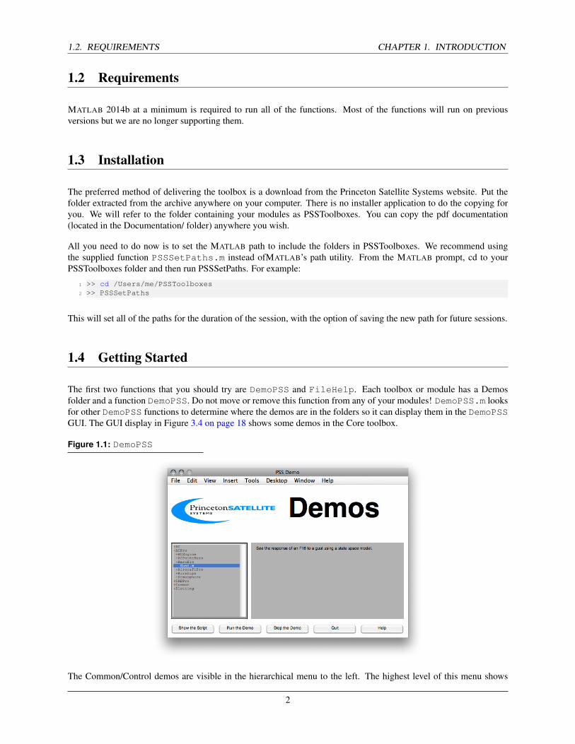
The first two functions that you should try are DemoPSS and FileHelp. Each toolbox or module has a Demosfolder and a function DemoPSS. Do not move or remove this function from any of your modules! DemoPSS.m looksfor other DemoPSS functions to determine where the demos are in the folders so it can display them in the DemoPSSGUI. The GUI display in Figure 3.4 on page 18 shows some demos in the Core toolbox.

Figure 1.1: DemoPSS

The Common/Control demos are visible in the hierarchical menu to the left. The highest level of this menu shows

2

CHAPTER 1. INTRODUCTION 1.4. GETTING STARTED

the folders within the toolbox. You can add your own demo scripts to the demo folders so that they can appear in thedisplay.

The FileHelp function, discussed in more detail in the next chapter, provides a graphical interface to the MATLABfunction headers. You can peruse the functions by folder to get a quick sense of your new product’s capabilitiesand search the function names and headers for keywords. FileHelp and DemoPSS provide the best way to get anoverview of the Aircraft Control Toolbox.

Another useful search tool is the Finder GUI. Type Finder at the prompt to initialize the GUI. A screenshot is shownin Figure 1.2 on the next page. This tool allows you to search for a string inside non-MATLAB m-files. You can lookover the entire path, or pick a single folder. You have the additional option of including all sub-folders recursively inthe search. You can decide whether to make the search case sensitive, and whether or not to look for the whole word.Whole words are separated by whitespace or any other non alpha-numeric character. In addition, we have included thenice feature of distinguishing between comments and code. You can search for the string ONLY in comments, ONLYin code, or in both.

Figure 1.2: Finder

3

1.4. GETTING STARTED CHAPTER 1. INTRODUCTION

4

CHAPTER 2

FUNDAMENTALS

This chapter gives you some basic information about the toolbox, including the aircraft properties database, classes,and code conventions.

2.1 Aircraft Properties Database

All aircraft properties are stored in databases that can be accessed through text-based commands. The toolbox comeswith a predefined database of aircraft properties. The following table lists all of the aircraft databases included in thetoolbox.

Table 2.1: Aircraft Properties

File Name Type DescriptionF16.m Nonlinear Tables of aerodynamic coefficients for a simplified F16 modelAIRC.m Statespace Vertical dynamics for an aircraftCCV .m Statepace Longitudinal dynamics for a control configured vehicle (CCV)DC8.m Stability Deriva-

tivesLongitudinal and lateral dynamics.

L1011.m Statespace Lateral dynamics for an airliner0H6A.m Statespace Longitudinal and lateral dynamics for a small helicopter in hover.STOVL.m Statespace Longitudinal and lateral dynamics for a Short Take-Off Vertical Landing (STOVL)

vehicle in hover and transition modesF18Model.m Statespace Longitudinal and lateral dynamics for an F/A-18 aircraft over a range of altitudes and

Mach numbers.CCVSObel.m Statespace CCV longitudinal aircraft model with a pitch pointing modeA10.m Statespace A10 aircraft models: with and without tiltable wing panels.F100.m Statespace Gas Turbine 16th-order F100 linear model: Pratt and Whitney F100-PW-100(3) con-

tinuous time model

The properties in a database are accessed by passing a text string to the database function. The text string identifiesthe set of properties or the dynamic mode that you want to obtain. You can first obtain a list of possible text stringidentifiers for the database by passing the argument ’catalog’. For example, to obtain the options for the STOVL.mfunction:

>> STOVL(’catalog’)ans =longitudinal hoverlateral/directional hover

5

2.2. CLASSES CHAPTER 2. FUNDAMENTALS

longitudinal transitionlateral/directional transition

Next, to obtain the statespace model associated with longitudinal hover:

>> g = STOVL(’longitudinal hover’)g =

statespace object: 1-by-1

You can then obtain information about this object of class statespace. For example, you can compute the eigen-values of the system by simply supplying g as an input to the eig function:

>> eig(g)ans =

0-0.014

0.30555502572409-0.214277512862045 + 0.297241130045908i-0.214277512862045 - 0.297241130045908i

-50-4

See the next section for more information on the statespace and acstate classes.

The usage of the F18Model.m function is slightly different. This database stores an array of longitudinal and lateral-directional dynamic statespace models across a range of flight conditions. It takes as inputs a Mach number andaltitude, which define a unique flight condition. The function then returns the statespace model associated with theclosest stored Mach number and altitude.

In addition to the aircraft databases listed above, the toolbox also provides the capability to generate dynamic modelsfor airships, or lighter-than-air vehicles. Rather than storing databases of aerodynamic properties, the airship modelingfunctions allow you to size an airship for operation at a desired altitude, and then automatically generate the massproperties and aerodynamic coefficients for your design. The airship functions are discussed in Section 11 on page 67.

2.2 Classes

The Aircraft Control Toolbox defines and makes use of the following two classes:

• acstate

• statespace

2.2.1 Class: acstate

The acstate class defines an aircraft state vector. At a minimum, it stores all of the usual information associatedwith a dynamic state vector for a rigid body, including the position, velocity, attitude, and body angular rates, as wellas the mass, CG location, and moment of inertia. It can also store additional information if necessary, including theangular velocity of rotors, and any number of states for engines, actuator, sensors, flexible dynamics, and disturbancemodels.

The “help” information on acstate.m explains how to create an acstate class object.

1 >> help acstate2 ---------------------------------------------------------------------------3 Create an object of class acstate

6

CHAPTER 2. FUNDAMENTALS 2.2. CLASSES

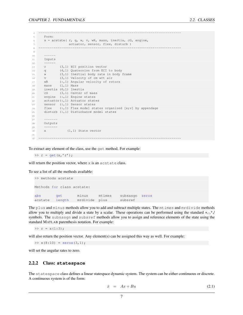
4 ---------------------------------------------------------------------------5 Form:6 x = acstate( r, q, w, v, wR, mass, inertia, cG, engine,7 actuator, sensor, flex, disturb )8 ---------------------------------------------------------------------------9

10 ------11 Inputs12 ------13 r (3,1) ECI position vector14 q (4,1) Quaternion from ECI to body15 w (3,1) Inertial body rate in body frame16 v (3,1) Velocity of cm wrt air17 wR (:,1) Angular velocity of rotors18 mass (1,1) Mass19 inertia (6,1) Inertia20 cG (3,1) Center of mass21 engine (:,1) Engine states22 actuator(:,1) Actuator states23 sensor (:,1) Sensor states24 flex (:,1) Flex model states organized [x;v] by appendage25 disturb (:,1) Disturbance model states26

27 -------28 Outputs29 -------30 x (1,1) State vector31

32 ---------------------------------------------------------------------------

To extract any element of the class, use the get method. For example:

>> r = get(x,’r’);

will return the position vector, where x is an acstate class.

To see a list of all the methods available:

>> methods acstate

Methods for class acstate:

abs get minus mtimes subsasgn zerosacstate length mrdivide plus subsref

The plus and minus methods allow you to add and subtract multiple states. The mtimes and mrdivide methodsallow you to multiply and divide a state by a scalar. These operations can be performed using the standard +,-,*,/symbols. The subsasgn and subsref methods allow you to assign and reference elements of the state using thestandard MATLAB parenthesis notation. For example:

>> r = x(1:3);

will also return the position vector. Any element(s) can be assigned this way as well. For example:

>> x(8:10) = zeros(3,1);

will set the angular rates to zero.

2.2.2 Class: statespace

The statespace class defines a linear statespace dynamic system. The system can be either continuous or discrete.A continuous system is of the form:

x = Ax+Bu (2.1)

7

2.2. CLASSES CHAPTER 2. FUNDAMENTALS

y = Cx+Du (2.2)

where x is the state vector, A is the state transition matrix, and B is the control effect matrix. Each system type isdenoted with a unique string identifier. Continuous systems are denoted with “s”.

For a discrete system, there are two different ways to write the state evolution. The first method is shown below, whichwe call the “z” method:

xk+1 = Axk +Buk (2.3)yk = Cxk +Duk (2.4)

The other discrete method uses the delta operator. This is termed the “delta” method:

xk+1 = xk +Axk +Buk (2.5)yk = Cxk +Duk (2.6)

A continuous statespace system can be converted to discrete-time by using the C2DZOH or C2DelZOH methods,which use a zero-order-hold on the input over a specified sampling time. The conversion from continuous to discretetime changes the A and B matrices only. The same C and D matrices are valid for both continuous and discretedomains.

To define a statespace class, you must at least specify the A,B,C matrices. If the D matrix is not supplied it isset to all zeros. In addition, you may also supply a name for the system, individual names for the states, inputs, andoutputs, the system type, and the time step (if the system is discrete). The “help” information on statespace.m explainshow to create an statespace class object.

1 >> help statespace2 -------------------------------------------------------------------------------3 Create a state space object. Everything after c is optional.4 -------------------------------------------------------------------------------5 Form:6 g = statespace( a, b, c, d, name, states, inputs, outputs, sType, dT )7 -------------------------------------------------------------------------------8

9 ------10 Inputs11 ------12 a State transition matrix13 b State input matrix14 c State output matrix15 d State feedthrough matrix16 name (1,:) Name of the system17 states (:,:) or {:} State names18 inputs (:,:) or {:} Input names19 outputs (:,:) or {:} Outputs20 sType (1,:) ’s’, ’z’, ’delta’21 dT (1,1) Time step22

23 -------24 Outputs25 -------26 g (:) Plant27 g.a State transition matrix28 g.b State input matrix29 g.c State output matrix30 g.d State feedthrough matrix31 g.n Number of states32 g.nI Number of inputs33 g.nO Number of outputs34 g.states Names of states35 g.inputs Names of inputs36 g.outputs Names of outputs

8

CHAPTER 2. FUNDAMENTALS 2.3. CODE CONVENTIONS

37 g.sType ’s’, ’z’, ’delta’38 g.dT Time step39

40 -------------------------------------------------------------------------------

You can view the methods associated with the statespace class by typing:

>> methods statespace

Methods for class statespace:

and connect get getsub mtimes seriesstatespace

close eig getabcd isempty plus set

Assume you have a statespace class named g. You can extract the A,B,C,D matrices from the class by typing:

>> [a,b,c,d] = getabcd(g);

Similarly, you can extract individual matrices or other information using the get method.

>> b = get(g,’b’);>> stateNames = get(g,’states’);

2.3 Code Conventions

It is important to follow consistent code conventions to make the code easy for other people to understand and use.The scripts and functions supplied with this toolbox are always supplied with a descriptive header that provides usagesyntax and a list of inputs and outputs. You can type

>> help FUNCTION

for any function to view the header.

When naming variables, we strive to use meaningful names. We also follow the C convention:

word1Word2Word3

where the beginning of each word after the first is capitalized. If a word is abbreviated the first letter is not capitalized.For example:

rPM

is revolutions per minute.

Almost all function names in ACT begin with a capital letter to distinguish them from variables. The only exceptionsare class methods, such as get and plus, for example. These method names overload built-in MATLAB functionsfor other class methods, and therefore must be all lower case.

Many functions in the Aircraft Control Toolbox can be executed with no inputs, even when inputs are required. If aninput is required but not provided, the function may use its own default value. You can see what the default valuesare by opening the function and examining the lines of code that immediately follow the help comments at the top ofthe file. For example, consider the AirshipControlDemo.m function. We see from the help header that it is called asfollows:

% Form:% out = AirshipControlDemo( alpha, beta, V, w0, alt, T, doPlot )

This function takes 7 inputs. Examining the file, we see that if no inputs are provided, it uses its own set of defaultvalues:

9

2.3. CODE CONVENTIONS CHAPTER 2. FUNDAMENTALS

if( nargin == 0 )alpha = 2*pi/180;beta = 1*pi/180;V = 24;w0 = [0;0;0];alt = 21336;T = 100;doPlot= [];

end

10

CHAPTER 3

GETTING HELP

This chapter shows you how to use the help systems built into PSS Toolboxes. There are several sources of help. Ourtoolboxes are now integrated into MATLAB’s built-in help browser. Then, there is the MATLAB help system whichprints help comments for individual files and lists the contents of folders. Also, there are special help utilities builtinto the PSS toolboxes: one is the file help function, the second is the demo functions and the third is the graphicaluser interface help system. Additionally, you can submit technical support questions through our website and use ourweb forums to join discussions about the toolboxes.

3.1 MATLAB’s Built-in Help System

3.1.1 Basic Information and Function Help

Our toolbox information can now be found in the MATLAB help system. To access this capability, simply open theMATLAB help system. As long as the toolbox is in the MATLAB path, it will appear in the contents pane. Its locationis depicted in Figure 3.1 (R2011b and earlier).

Figure 3.1: MATLAB Help

11

3.2. MATLAB HELP CHAPTER 3. GETTING HELP

This contains a lot information on the toolbox. It also allows you to search for functions as you would if you weresearching for functions in the MATLAB root.

3.1.2 Published Demos

Another feature that has been added to the MATLAB help structure is the access to all of the toolbox demos. Everysingle demo is now listed, according to module and the folder. These can be found under the Other Demos or Examplesportion of the Contents Pane. Each demo has its own webpage that goes through it step by step showing exactly whatthe script is doing and which functions it is calling. From each individual demo webpage you can also run the scriptto view the output, or open it in the editor. Note that you might want to save any changes to the demo under a new filename so that you can always have the original. Below is an example of demo page displayed in MATLAB help thatshows where to find the toolbox demos as well as the the hierarchal structure used for browsing the demos.

Figure 3.2: Toolbox Demos

3.2 MATLAB Help

You can get help for any function by typing

>> help functionName

12

CHAPTER 3. GETTING HELP 3.2. MATLAB HELP

For example, if you type

>> help C2DZOH

you will see the following displayed in your MATLAB command window:1 -----------------------------------------------------------------2 Create a discrete time system from a continuous system3 assuming a zero-order-hold at the input.4 Given5 .6 x = ax + bu7

8 Find f and g where9 x(k+1) = fx(k) + gu(k)

10

11 -----------------------------------------------------------------12 Form:13 [f, g] = C2DZOH( a, b, T )14 -----------------------------------------------------------------15 ------16 Inputs17 ------18 a Plant matrix19 b Input matrix20 T Time step21 -------22 Outputs23 -------24 f Discrete plant matrix25 g Discrete input matrix26

27 -----------------------------------------------------------------

All PSS functions have the standard header format shown above. Keep in mind that you can find out which folder afunction resides in using the MATLAB command which, i.e.

>> which C2DZOH/Software/Toolboxes/Aerospace/Common/Control/C2DZOH.m

When you want more information about a folder of interest, remember that you can get a list of the contents in anydirectory by using the help command with a folder name. The returned list of files is organized alphabetically. Forexample,

>> help ACDynamics

ACDynamics

AAC - Dynamics model for an aircraft. Updates

the data structure x.ACBuild - Build the aircraft model.ACInit - Initialize the aircraft model.ACPlot - Plots the aircraft data. opt is ’info’, ’

init’, ’store’, ’plot’ACTrim - Aircraft trimming algorithm. Uses the

function FTrim. This algorithm

FFTrim - Cost function for the trimming algorithm

SStateSpacePlot - Plots statespace data. opt is ’init’, ’

store’, ’plot’

13

3.2. MATLAB HELP CHAPTER 3. GETTING HELP

If there is a folder with the same name in a Demos directory, the demos will be listed separately. For example,

>> help AeroPro

Demos/AeroPro

GGust - See the response of an F16 to a gust using

a state space model.

AeroPro

HHorizontalWind - Form:

WWindGust - Wind gust model. Generates state space

equations or spectral densities.

This type of help also works with higher level directories, for instance if you ask for help on the Common directory,you will get a list of all the subdirectories.

PSS Toolbox Folder CommonVersion 2014.1 11-Jul-2014

Directories:AtmosphereClassesCommonDataControlControlGUIDatabaseDemoFunsDemosDemos/ControlDemos/ControlGUIDemos/DatabaseDemos/GeneralDemos/GeneralEstimationDemos/GraphicsDemos/HelpDemos/MassPropertiesDemos/PluginsDemos/UKFEstimationFileUtilsGeneralGraphicsHelpInterfaceMassPropertiesMaterialsPluginsQuaternionTimeTransform

The function ver lists the current version of all your installed toolboxes. Each ACT module that you have installedwill be listed separately. For instance,

14

CHAPTER 3. GETTING HELP 3.3. FILEHELP

-------------------------------------------------------------------------------------

MATLAB Version: 8.1.0.604 (R2013a)...-------------------------------------------------------------------------------------

MATLAB Version 8.1 (R2013a)PSS Toolbox Folder AC Version 2014.1PSS Toolbox Folder ACPro Version 2014.1PSS Toolbox Folder AeroUtils Version 2014.1PSS Toolbox Folder Airships Version 2014.1PSS Toolbox Folder Common Version 2014.1PSS Toolbox Folder Math Version 2014.1PSS Toolbox Folder Plotting Version 2014.1

3.3 FileHelp

3.3.1 Introduction

When you type

FileHelp

the FileHelp GUI appears.

Figure 3.3: The file help GUI

15

3.3. FILEHELP CHAPTER 3. GETTING HELP

There are five main panes in the window. On the left hand side is a display of all functions in the toolbox arrangedin the same hierarchy as the PSSToolboxes folder. Scripts, including most of the demos, are not included. Belowthe hierarchical list is a list in alphabetical order by product. On the right-hand-side is the header display pane.Immediately below the header display is the editable example pane. To its left is a template for the function. You cancut and paste the template into your own functions.

3.3.2 The List Pane

If you click a file in the alphabetical or hierarchical lists, the header will appear in the header pane. This is the sameheader that is in the file. The headers are extracted from a .mat file so changes you make will not be reflected in thefile. In the hierarchical list, any name with a + or - sign is a folder. Click on the folders until you reach the file youwould like. When you click a file, the header and template will appear.

3.3.3 Edit Button

This opens the MATLAB edit window for the function selected in the list.

3.3.4 The Example Pane

This pane gives an example for the function displayed. Not all functions have examples. The edit display has scrollbars. You can edit the example, create new examples and save them using the buttons below the display. To run anexample, push the Run Example button. You can include comments in the example by using the percent symbol.

3.3.5 Run Example Button

Run the example in the display. Some of the examples are just the name of the function. These are functions withbuilt-in demos. Results will appear either in separate figure windows or in the Matlab Command Window.

3.3.6 Save Example Button

Save the example in the edit window. Pushing this button only saves it in the temporary memory used by the GUI.You can save the example permanently when you Quit.

3.3.7 Help Button

Opens the on-line help system.

3.3.8 Quit

Quit the GUI. If you have edited an example, it will ask you whether you want to save the example before you quit.

16

CHAPTER 3. GETTING HELP 3.4. SEARCHING IN FILE HELP

3.4 Searching in File Help

3.4.1 Search File Names Button

Type in a function name in the edit box and push Search File Names.

3.4.2 Find All Button

Find All returns to the original list of the functions. This is used after one of the search options has been used.

3.4.3 Search Headers Button

Search headers for a string. This function looks for exact, but not case sensitive, matches. The file display displays allmatches. A progress bar gives you an indication of time remaining in the search.

3.4.4 Search String Edit Box

This is the search string. Spaces will be matched so if you type attitude control it will not match attitude control (withtwo spaces.)

3.5 DemoPSS

If you type DemoPSS you will see the GUI in Figure 3.4 on the following page. The list on the left-hand-side ishierarchical and the top level follows the organization of your toolbox modules. Most folders in your modules havematching folders in Demos with scripts that demonstrate the functions. The GUI checks to see which directories arein the same directory as DemoPSS and lists all directories and files. This allows you to add your own directories anddemo files.

Click on the first name to open the directory. The + sign changes to - and the list changes. Figure 3.4 on the nextpage shows the ACPro/AeroPro folder, which has one demo: Gust.m. The hierarchical menu shows the highest levelfolders.

Your own demos will appear if they are put in any of the Demos folders. If you would like to look at, or edit, the script,push Show the Script.

3.6 Graphical User Interface Help

Many of the graphical user interfaces (GUI) have a help button. If you hit the help button a new window will appearwhich displays information about how to use the GUI. You can access on-line help about the GUIs through this display.It is separate from the file help GUI described above. The display is hierarchical. Any list item with a + or - in front isa help heading with multiple subtopics. + means the heading item is closed, - means it is open. Clicking on a headingname toggles it open or closed. Figure 3.5 on page 19 shows the display with the Telemetry help expanded. If youclick on a topic in the list you will get a text display in the right-hand pane. You can either search the headings or thetext by entering a text string into the Search For edit box and hitting the appropriate button. Restore List restores thelist window to its previous configuration.

17

3.7. TECHNICAL SUPPORT CHAPTER 3. GETTING HELP

Figure 3.4: The demo GUI

3.7 Technical Support

Contact support@psatellite.com for free email technical support. We are happy to add functions and demos for ourcustomers when asked.

18

CHAPTER 3. GETTING HELP 3.7. TECHNICAL SUPPORT

Figure 3.5: On-line Help

19

3.7. TECHNICAL SUPPORT CHAPTER 3. GETTING HELP

20

CHAPTER 4

COORDINATE TRANSFORMATIONS

This chapter shows you how to use Aircraft Control Toolbox functions for coordinate transformations.

4.1 Coordinate Frames

The guidance, navigation and control of aircraft require vectors to be expressed in several different coordinate frames.The fundamental coordinate frames of interest are:

• Body-fixed (BODY)

• Stability-axis (STAB)

• Wind-axis (WIND)

• North-East-Down (NED)

• Earth-Centered Inertial (ECI)

Each coordinate frame is an orthogonal right-handed system. The BODY, STAB, and WIND frames are all attachedto a fixed point on the aircraft. The NED frame is attached to the surface of the Earth, while the ECI frame is anon-rotating inertial frame attached to the center of the Earth.

In the body-fixed coordinate frame, the x axis points forward out the nose, the y axis points out the right side of theaircraft, and the z axis completes the right-hand-system, pointing locally up. The rotational motion of the aircraft isdefined in the body frame as roll, pitch, and yaw about the x, y and z axes, respectively.

In the stability axis system (STAB), the y axis is aligned with the BODY frame y axis. The x−z plane is rotated aboutthe y axis through the angle of attack, α.

We go from STAB frame to the WIND frame by rotating about the z axis through the sideslip angle, β. The result isthat the x axis of the WIND frame is aligned exactly with the wind-relative velocity vector. In level flight, with noangle of attack and no sideslip angle, the STAB and WIND frames are both aligned exactly with the BODY frame.

A positive angle of attack rotates the stability x axis down, around the −y axis. A positive sideslip angle rotates the yaxis forward, around the −z axis.

The North-East-Down frame is attached to the surface of the Earth, on the line that connects the center of the Earth tothe aircraft. Expressing the aircraft velocity in the NED frame allows us to compute the heading and flight path angles.

21

4.2. TRANSFORMATION MATRICES CHAPTER 4. COORDINATES

The ECI frame is the inertial frame used for integrating the equations of motion.

4.2 Transformation Matrices

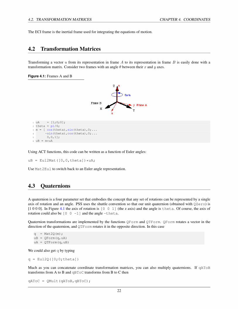
Transforming a vector u from its representation in frame A to its representation in frame B is easily done with atransformation matrix. Consider two frames with an angle θ between their x and y axes.

Figure 4.1: Frames A and B

1 uA = [1;0;0];2 theta = pi/6;3 m = [ cos(theta),sin(theta),0;...4 -sin(theta),cos(theta),0;...5 0,0,1];6 uB = m*uA

Using ACT functions, this code can be written as a function of Euler angles:

uB = Eul2Mat([0,0,theta])*uA;

Use Mat2Eul to switch back to an Euler angle representation.

4.3 Quaternions

A quaternion is a four parameter set that embodies the concept that any set of rotations can be represented by a singleaxis of rotation and an angle. PSS uses the shuttle convention so that our unit quaternion (obtained with QZero) is[1 0 0 0]. In Figure 4.1 the axis of rotation is [0 0 1] (the z axis) and the angle is theta. Of course, the axis ofrotation could also be [0 0 -1] and the angle -theta.

Quaternion transformations are implemented by the functions QForm and QTForm. QForm rotates a vector in thedirection of the quaternion, and QTForm rotates it in the opposite direction. In this case

q = Mat2Q(m);uB = QForm(q,uA)uA = QTForm(q,uB)

We could also get q by typing

q = Eul2Q([0;0;theta])

Much as you can concatenate coordinate transformation matrices, you can also multiply quaternions. If qAToBtransforms from A to B and qBToC transforms from B to C then

qAToC = QMult(qAToB,qBToC);

22

CHAPTER 4. COORDINATES 4.4. TRANSFORMATION FUNCTIONS

The transpose of a quaternion is just

qCToA = QPose(qAToC);

You can extract Euler angles by

eAToC = Q2Eul(qAToC);

or matrices by

mAToC = Q2Mat(qAToC);

If we convert the three Euler angles to a quaternion

qIToB = Eul2Q(e);

qIToB will transform vectors represented in I to vectors represented in B. This quaternion will be the transpose ofthe quaternion that rotates frame B from its initial orientation to its final orientation or

qIToB = QPose(qBInitialToBFinal);

Given a vector of small angles eSmall that rotate from vectors from frame A to B, the transformation from A to Bis

uB = (eye(3)-SkewSymm(eSmall))*uA;

where

1 SkewSymm([1;2;3])2 ans =3 [0 -3 2;4 3 0 -1;5 -2 1 0]

Note that SkewSymm(x)*y is the same as Cross(x,y).

4.4 Transformation Functions

The Aircraft Control Toolbox provides several useful functions to perform a variety of common coordinate transfor-mations. To see a summary, type:

>> help ACCoordAC/ACCoord

AAlphBeta - Compute angle of attack and sideslip.

BBToS - Convert from the body axes to stability

axes.BToW - Convert from the body frame to wind axes.

EECIToNED - Convert from the ECI frame to the NED

frame.EulNED - Euler angles given ECI information.EulRate - Euler rates.

23

4.4. TRANSFORMATION FUNCTIONS CHAPTER 4. COORDINATES

JJacobVB - Convert from the body axes to stability

axes.

QQECI - Compute ECI to body quaternion from ECI

position and Euler angles.

RRNEH - Convert from the ECI frame to the NEH

frame. This is the

SSToW - Convert from stability axes to wind axes.

VVBDToVBT - Compute the total velocity derivative from

the body velocity andVTToVB - Compute body velocity from alpha, beta and

vT.

In addition to these aircraft-specific coordinate functions, a wide range of general coordinate transformation routinesare available in the Common/Coord/ directory. For example, to compute the rotation matrix from the NED frame tothe BODY frame, use the Eul2Mat.m function.

>> rx = 0; % roll>> ry = 0.1; % pitch>> rz = pi/4; % yaw>> m = Eul2Mat( [rx;ry;rz] ); % NED to BODY matrix

The Euler angles are the rotations about the x, y, and z axes, respectively, which correspond to roll, pitch and yaw. Thematrix is computed by performing a 3-2-1 rotation sequence, where the first rotation is through the yaw angle aboutthe 3-axis (z), then through the pitch angle about the 2-axs (y), and finally through the roll angle about the 1-axis (x).

24

CHAPTER 5

ENVIRONMENT

This chapter describes the functions for atmospheric properties and wind models.

5.1 Atmospheric Properties

The standard atmosphere model is stored as a lookup table in the toolbox. The values of temperature, density, pressure,speed of sound and kinematic viscosity are indexed by altitude. The data spans from sea-level to 80 km. To load themodel into the workspace:

>> atmData = load(’AtmData.txt’);

To obtain the atmospheric properties at a desired altitude (i.e. 3000 meters), use the StdAtm.m function:

>> d = StdAtm( 3000, atmData, ’si’ )d =

temperature: 268.67pressure: 70121density: 0.90926

speedOfSound: 328.58kinematicViscosity: 1.8628e-05

The ’si’ string specifies the units to be in SI system. Alternatively, you can use the English system. In this case, thealtitude is entered in feet:

>> d = StdAtm( 3000/0.3048, atmData, ’eng’ )d =

temperature: 483.606pressure: 1464.58050086331density: 0.00176421019887722

speedOfSound: 1078.01837270341kinematicViscosity: 0.000200510123242469

The units are shown inside the StdAtm.m file.

% x is [altitude (m) temperature (deg-K) pressure (N/mˆ2) density (kg/mˆ3)% speed of sound (m/s) kinematic viscosity (mˆ2/s)]% or% [altitude (ft) temperature (deg-R) pressure (lbf/ftˆ2) density (lbf/mˆ3)% speed of sound (ft/s) kinematic viscosity (ftˆ2/s)]

Typing StdAtm creates plots that show the variation of the properties over altitude.

25

5.2. WIND MODELS CHAPTER 5. ENVIRONMENT

Figure 5.1: Standard Atmosphere Plots

Standard Atmosphere

0 1 2 3 4 5 6 7 8

x 104

0

0.5

1

1.5

Den

sity

(kg

/m3 )

0 1 2 3 4 5 6 7 8

x 104

150

200

250

300

Tem

pera

ture

(de

g−K

)

0 1 2 3 4 5 6 7 8

x 104

0

5

10

15x 10

4

Pre

ssur

e (N

/m2 )

Altitude (m)

Standard Atmosphere

0 1 2 3 4 5 6 7 8

x 104

280

300

320

340

360

Spe

ed o

f sou

nd (

m/s

)

0 1 2 3 4 5 6 7 8

x 104

0

0.2

0.4

0.6

0.8

1

Kin

emat

ic v

isco

sity

(m

2 /s)

Altitude (m)

Additional atmospheric functions can be found the AC/Aero folder.

>> help AeroAC/Aero

AADC - Implements the "Air Data Computer" model.AirData - Computes air data based on a simplified

standard atmosphere model. IfAtmGamma - Computes the ratio of specific heats as a

function of

MMachFromPressureRatio - Computes the Mach number from pressure

ratio.

PPressureRatioFromMach - Computes the ratio of impact to static

pressure from Mach number and gamma.

RReynolds - Compute the Reynolds number for an

aircraft at altitude.

SSimpAtm - Simplified atmosphere model. Agrees with

the standard

VViscosity - Compute the viscosity of the air at a

given temperature.

5.2 Wind Models

The toolbox provides a generic wind gust model and a steady state horizontal wind model. To see a summary of thefunctions:

>> help AeroPro

26

CHAPTER 5. ENVIRONMENT 5.2. WIND MODELS

ACPro/AeroPro

HHorizontalWind - Form:

WWindGust - Wind gust model. Generates state space

equations or spectral densities.ACPro/Demos/AeroPro

GGust - See the response of an F16 to a gust using

a state space model.

The Gust demo simulates a linearized model of the F16 with randomized wind gusts. For more information view thehelp for the Gust and WindGust functions.

The HorizontalWind function implements the HWM93 model. This is an empirical model developed by the NavalResearch Laboratory, originally written in FORTRAN. Typing HorizontalWind with no inputs runs a demo thatcreates a text file output. The model provides a steady-state average horizontal wind given the year, date, time of day,altitude, latitude and longitude, solar flux and magnetic index.

The WindLatLon function (also discussed in Chapter 11) provides a simpler interface to the horizontal wind model,taking only latitude, longitude, altitude, day of year and time of day. Plots from the built-in demo are shown below.The plots show the wind magnitude and direction at 70 thousand feet over a latitude and longitude range that coversthe U.S.

Figure 5.2: WindLatLon Demo

30 35 40 45 504

5

6

7

8

9

10

11

12

latitude [deg]

|W|[m/s]

long = −120long = −115long = −110long = −105long = −100long = −95long = −90long = −85long = −80long = −75long = −70

30 35 40 45 50−95

−94.5

−94

−93.5

−93

−92.5

−92

−91.5

latitude [deg]

Ψ[deg]

long = −120long = −115long = −110long = −105long = −100long = −95long = −90long = −85long = −80long = −75long = −70

The WindsGUI tool provides a visual interface for the horizontal wind model. It is shown in Figure 5.3 on thefollowing page. Use it to generate wind data over an array of different conditions, and then visualize the results witha 3D surface plot and sliders to vary additional parameters. You can also save the data that you generate to a file, andload existing files into the GUI. Once you have saved a file, you can use the WindTrendsDemo function to generatean animation of the wind behavior over a selected variable.

27

5.2. WIND MODELS CHAPTER 5. ENVIRONMENT

Figure 5.3: WindsGUI

28

CHAPTER 6

SIMULATION

6.1 Aircraft Simulations

6.1.1 Introduction

It is convenient and practical for us to differentiate between linear and nonlinear simulations. Aircraft dynamics areinherently nonlinear, and most aircraft actuators and sensors are nonlinear as well. Nonetheless, it is usually possibleto linearize the dynamics and devices about some operating point where, in a sufficient restricted region around thispoint, the system behaves linearly. This is the basis for the linear control laws developed in this toolbox. The toolboxuses the function AC.m for all nonlinear aircraft simulations. The same function can also be used to develop linearmodels at specific operating conditions. With appropriate plug-in functions, it can perform sophisticated simulationsof anything from a biplane to a single-stage-to-orbit launch vehicle.

6.1.2 Aspects of Simulation Models

Aircraft simulations can range from simple 3 DOF longitudinal dynamic models to models that incorporate the dy-namics of moving parts, aero-elasticity, dynamical engine models, pilot dynamics, and so forth. There are two majortools for simulation in the toolbox. One is to use the statespace models for linear simulations. The other is to use thenonlinear simulation, AC.m.

Two convenient statespace simulation tools are Step.m and IC.m. They do step responses and unforced responsesto an initial state, respectively. Another useful tool is MSR.m, which computes mean squared responses of a system tonoise inputs.

The following table lists different features that simulation models can have and shows which ones are available inAC.m.

Table 6.1: Breakdown of Simulation Models

Feature InAC?

Description Uses

Rigid Body (6DOF) Yes 3 rotational and 3 translational degrees of freedom. 6 kinematic states (7 ifquaternions are used).

All aircraft

Flat Earth Yes Constant gravity. No Earth curvature. Most aircraftEllipsoidal Earth Yes Includes rotation of the Earth, altitude dependent gravity, and latitude dependent

Earth radius.Launch vehicles.

29

6.1. AIRCRAFT SIMULATIONS CHAPTER 6. SIMULATION

Table 6.1: Simulation Models, contd.

Feature InAC?

Description Uses

Rotating Parts Yes Spinning parts, such as gas turbines or a gatling gun on an A-10. All aircraft with en-gines.

Actuator Dynamics Yes Linear and/or nonlinear models that relate commanded thrust, deflection, etc. tothe actual value. Accommodates lags, delays, limits.

All aircraft but notalways necessaryfor preliminarydesigns.

Sensor Dynamics Yes Nonlinear models that relate measured quantity to the output measurement. See above.Flexible modes Yes Bending of wings, etc. Important for eval-

uating aero-elasticeffects.

Time varying iner-tia and mass

Yes For launch vehicles, the inertia, CG and mass change as fuel is consumed. Forlighter-than-air vehicles, the mass properties change as internal gasbags inflateand deflate with changing altitude.

Launch vehicles,lighter-than-airvehicles.

Added mass and in-ertia

Yes For lighter-than-air vehicles, the added (or “apparent”) mass and inertia that mustbe modeled to account for momentum of the displaced fluid through which thevehicle moves.

Lighter-than-air ve-hicles.

Inertia and mass ofmoving parts

No On some aircraft (and on boosters with large gimballed nozzle assemblies) thedynamics of moving parts can be significant.

Light aircraft andsome boosters.

Detachable parts No Bombs and missiles. Military aircraft.Thermal effects No Interaction of heating and aerodynamics. Supersonic aircraft.

Re-entry vehicles.

Two demos show how to use AC.m with the F16.m database. The rst is CTSim.m which simulates a coordinatedturn. The second is Fly.m which lets you y the F16 using the head up display, HUD.m. The steps you take to set upa simulation are:

1. Trim the model using ACTrim.m.

2. Initialize the model data structures and state vector using ACBuild.m and ACInit.m.

3. Run AC.m.

4. Get plot results with ACPlot.m.

6.1.3 Simulating Linear Systems

Creating a State Space System

If you have your model in transfer function form it can be converted to state space form using

[a,b,c,d] = ND2SS( num, den );

The variable num can have more than one row. To make it of type statespace

g = statespace( a, b, c, d );

If you have a nonlinear system expressed in the form and f is a MATLAB function in the form

xDot = F(x,u);

then

[a,b] = Jacobian(’f’,x,u);

30

CHAPTER 6. SIMULATION 6.1. AIRCRAFT SIMULATIONS

Discrete-Time Systems

The simplest way to simulate a continuous time system is to discretize it using the zero order hold. This toolbox givestwo ways to do this. One is the standard zero order hold

[aD,bD] = C2DZoh(a,b,T);

and the simulation is

x = aD*x + bD*u;y = c*x + d*u;

The second is the delta form of the zero order hold

[aD,bD] = C2DelZoh(a,b,T);

and the simulation is

x = x + aD*x + bD*u;y = c*x + d*u;

These approximations assume that the input is held constant over the interval T.

Time Response

The time response of a statespace system is easily obtained using ACT functions. To generate an unforced response toinitial conditions, use IC.m The usage is:

[y, x] = IC( g, x0, dT, nSim )

where g is the statespace system, x0 is the initial state, dT is the time step, and nSim is the number of points tosimulate.

If you have a discrete system, g, you can compute the time response to a given control history as follows:

[x, y] = PropStateSpace( g, x0, u )

where x0 is the initial state, and u is the control history. u is a M × N matrix, where M is the number of controlsand N is the number of timesteps. The time between timesteps is assumed to be equal to the sampling period of thediscrete system.

Alternatively, you can use the TResp function. This function works for either a continuous or discrete system.

[x,y,t,u] = TResp( g, x0, u, dT, T );

Here, T is the simulation duration and dT is the time interval of the simulation. The time interval should be equal tothe sampling period if the system is discrete. As an option, the control vector u can be supplied as empty, or with justone column. If it is supplied empty, all inputs will be set to 1 for all time. If it is supplied with one column, those inputvalues will be applied for all time.

You can use the Step.m function to compute the response to unit step, impulse, or white noise inputs. The usage is:

[y,x,t] = Step( g, iU, dT, nSim, inputType, statesFlag )

where g is the statespace system, iU is the index (row) of the input to use (all other inputs are set to zero), dT is thesimulation time interval, nSim is the number of simulation points, inputType is a string for either ‘step’, ‘impulse’,or ‘white noise’. This is an optional input that defaults to ‘step’. The final input statesFlag is also optional; it is aflag to indicate whether to generate time-history plots of all the states. By default the value is 1 and the plots are made.

Frequency Response

A variety of tools are available to generate and plot the frequency response of a linear system as well. Consider alinear system, g. The statespace system can be created as follows:

31

6.1. AIRCRAFT SIMULATIONS CHAPTER 6. SIMULATION

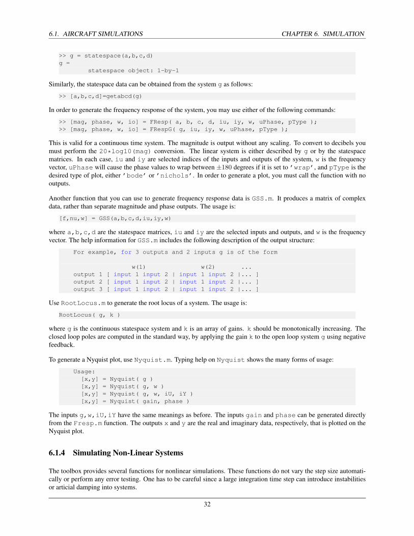
>> g = statespace(a,b,c,d)g =

statespace object: 1-by-1

Similarly, the statespace data can be obtained from the system g as follows:

>> [a,b,c,d]=getabcd(g)

In order to generate the frequency response of the system, you may use either of the following commands:

>> [mag, phase, w, io] = FResp( a, b, c, d, iu, iy, w, uPhase, pType );>> [mag, phase, w, io] = FRespG( g, iu, iy, w, uPhase, pType );

This is valid for a continuous time system. The magnitude is output without any scaling. To convert to decibels youmust perform the 20*log10(mag) conversion. The linear system is either described by g or by the statespacematrices. In each case, iu and iy are selected indices of the inputs and outputs of the system, w is the frequencyvector, uPhase will cause the phase values to wrap between ±180 degrees if it is set to ’wrap’, and pType is thedesired type of plot, either ’bode’ or ’nichols’. In order to generate a plot, you must call the function with nooutputs.

Another function that you can use to generate frequency response data is GSS.m. It produces a matrix of complexdata, rather than separate magnitude and phase outputs. The usage is:

[f,nu,w] = GSS(a,b,c,d,iu,iy,w)

where a,b,c,d are the statespace matrices, iu and iy are the selected inputs and outputs, and w is the frequencyvector. The help information for GSS.m includes the following description of the output structure:

For example, for 3 outputs and 2 inputs g is of the form

w(1) w(2) ...output 1 [ input 1 input 2 | input 1 input 2 |... ]output 2 [ input 1 input 2 | input 1 input 2 |... ]output 3 [ input 1 input 2 | input 1 input 2 |... ]

Use RootLocus.m to generate the root locus of a system. The usage is:

RootLocus( g, k )

where g is the continuous statespace system and k is an array of gains. k should be monotonically increasing. Theclosed loop poles are computed in the standard way, by applying the gain k to the open loop system g using negativefeedback.

To generate a Nyquist plot, use Nyquist.m. Typing help on Nyquist shows the many forms of usage:

Usage:[x,y] = Nyquist( g )[x,y] = Nyquist( g, w )[x,y] = Nyquist( g, w, iU, iY )[x,y] = Nyquist( gain, phase )

The inputs g,w,iU,iY have the same meanings as before. The inputs gain and phase can be generated directlyfrom the Fresp.m function. The outputs x and y are the real and imaginary data, respectively, that is plotted on theNyquist plot.

6.1.4 Simulating Non-Linear Systems

The toolbox provides several functions for nonlinear simulations. These functions do not vary the step size automati-cally or perform any error testing. One has to be careful since a large integration time step can introduce instabilitiesor articial damping into systems.

32

CHAPTER 6. SIMULATION 6.2. CREATING AN INTERACTIVE SIMULATION

The Aircraft Control Toolbox also provides a variable step size routine, RK45, and Euler, a rst order method.

Given the function

xDot = Fun(x,t,p1,p2...p10)

and time step h use either

x = RK2( Fun , x, h, t, p1, p2, p3, p4, p5, p6, p7, p8, p9, p10 );

or

x = RK4( Fun , x, h, t, p1, p2, p3, p4, p5, p6, p7, p8, p9, p10 );

The variables t (time) and p1 through p10 are optional arguments. If you need more than 10 optional arguments youcan pack p1 through p10. For example if you need to pass two inertia matrices

p1 = [inertia1,inertia2];

6.2 Creating an Interactive Simulation

Fly.m is a complete, nonlinear, interactive simulation that uses all of the toolbox GUIs to allow you to y an F-16.

In this section we walk through the script Fly.m and explain in detail how it works. A summary of how to set upsimulation scripts has already been given above so we will jump right into the details.

Listing 6.1: Main Initialization Fly.m

% Global for the time GUI%------------------------global simulationActionsimulationAction = ’ ’;

% Global for the HUD%-------------------global hUDOutputhUDOutput = struct(’pushbutton1’,0,’pushbutton2’,0,’checkbox1’,0,...

’checkbox2’,0,’checkbox3’,0);

% load the F16 database%----------------------d = DefaultACData;

% Load the Trim State and Control Settings (found via ACTrim)%-----------------------------------------trimData.x = DefaultACState;trimData = load(’F16TrimData.mat’);d.control = trimData.control;x = trimData.x;

% Time%-----t = 0;dT = 0.1;nSim = 200/dT;

% Initialize the model%---------------------d = ACInit( x, d );

Fly.m

In Listing 6.1, we first define the global variables for the graphical interfaces, TimeGUI.m and HUD.m. We thenload the aircraft data structure, d, using DefaultACData. This returns a data structure with a standard atmosphere

33

6.2. CREATING AN INTERACTIVE SIMULATION CHAPTER 6. SIMULATION

model and the F16 aerodynamic model. Next, the trim state and controls are loaded. The time step is then set to 0.1sec and the number of integration steps are computed. Finally, the full simulation data structure d is initialized usingACInit. This function returns the original data structure along with new fields for generalized inertia, rotor data,flexible model data, and state names.

The DefaultACData.m function is shown in Listing 6.2. In the first block of code, it loads the F16 aerodynamicmodel data, and initializes the planet angle and angular rate (in this case we ignore planet rotation). It then spec-ifies which functions are to be used for actuator, aerodynamic, engine, rotor, sensor and disturbance models. Thename elds are names of functions that implement these different models. The files ACAero.m, ACEngine.m andACSensor.m are models included with the toolbox. You can write your own models and use AC.m as the simula-tion engine, as long as you adhere to the input/output conventions for each of the functions. Type help AC for moreinformation.

The middle block of code loads data for the standard atmosphere and species the units as English (ft.). The last codeblock initializes the controls. The actual control values can be changed at any time of course, before or during thesimulation.

Listing 6.2: Default Aircraft Models and Controls DefaultACData.m

% F16 database%-------------d = ACBuild(’F16’);d.theta0 = 0;d.wPlanet = [0;0;0];d.actuator.name = [];d.aero.name = ’ACAero’;d.engine.name = ’ACEngine’;d.rotor.name = [];d.sensor.name = ’ACSensor’;d.disturb.name = [];

% Load the standard atmosphere%-----------------------------d.atmData = load(’AtmData.txt’);d.atmUnits = ’eng’;

% Control%--------d.control.throttle = .155;d.control.elevator = -2.5574984;d.control.aileron = -1.27e-6;d.control.rudder = 2.134e-5;

DefaultACData.m

The state vector loaded in using the DefaultACState.m function. It is specied in terms of angle-of-attack(alpha), sideslip (beta) and total velocity, vT. These are converted in to body state vector by VTToVB. The cG,inertia and mass are also states and are specied. The simulation uses quaternions and QECI converts the initialeuler angles and position vector to the quaternion from ECI to the body frame. The engine model has a single state.In this case a default value is provided, but the equilibrium value can be found by using ACEngEq, which takes theaircraft data structure (containing the control) and nds the engine equilibrium state at that control setting. There are noactuator, sensor, ex or disturbance states so they are set to empty matrices.

Once all of the data is set the data structure of type acstate is created using the constructor acstate.

Listing 6.3: Default State Data DefaultACState.m

% default state data%-------------------alpha = 0.03691;beta = -4e-9;vT = 502;v = VTToVB( vT, alpha, beta );cG = [0.35;0;0];

34

CHAPTER 6. SIMULATION 6.2. CREATING AN INTERACTIVE SIMULATION

r = [2.092565616797901e+07;0;0];eulInit = [0;0.03691;0];qNEDToB = Eul2Q(eulInit);qECIToNED = ECIToNED( r, ’quaternion’ );q = QMult( qECIToNED, qNEDToB );w = [0;0;0];wR = 160;mass = 1/1.57e-3;inertia = [9497;55814;63100;0;-982;0];engine = 8.99419;actuator = [];sensor = [];flex = [];disturb = [];

% Initialize state object%------------------------x = acstate( r, q, w, v, wR, mass, inertia, cG, engine, actuator, sensor, flex, disturb );

DefaultACState.m

The trim control data for this aircraft state has been pre-computed and stored in the mat-file, F16TrimData.mat.Alternatively, the trim controls for a new state can be computed using the ACTrim.m function. Type “helpACTrim” for usage information.

Now we return to Fly.m. We have already initialized the state, models, and controls. Next, the linearized plant modelis computed, just for informational purposes. The function ACModes extracts the standard aircraft rigid body modes.Note that ACModes is only valid if the aircraft is flying straight and level.

Listing 6.4: Linearized Model Fly.m

% Compute the linearized model%-----------------------------gLin = AC( x, 0, 0, d, ’linalpha’);aC = get( gLin, ’a’ );

% Display aircraft rigid body modes%----------------------------------ACModes( gLin );

Fly.m

Next the two main graphical interfaces are initialized: the heads up display (HUD) and the 3D CAD model window.These displays are discussed more in Section 6.4 on page 38. The settings for maximum controls are used to convertmouse movement into control values.

Listing 6.5: Setting up the HUD and 3D Aircraft Display Fly.m

% Set up the HUD%---------------dHUD.atmData = d.atmData ;dHUD.atmUnits = ’eng’;

cHUD.control = d.control;cHUD.elevatorMax = 90;cHUD.aileronMax = 90;cHUD.rudderMax = 90;cHUD.dT = dT;hHUD = HUD( ’init’, dHUD, x, [], cHUD );

% Set up the aircraft display%----------------------------gF16 = load( ’gF16’ )hF16 = DrawAC( ’init’, gF16, x, [], d.atmUnits );

Fly.m

Plotting is initialized by specifying the names of plots. ACPlot.m lists all available plots. The time display is

35

6.2. CREATING AN INTERACTIVE SIMULATION CHAPTER 6. SIMULATION

discussed in the graphics section.

Listing 6.6: Initializing ACPlot.m Fly.m

% Initialize the plots%---------------------plots = [ ’Euler angles ’;...

’Quaternion ’;...’Quaternion NED To B’;...’Angular rate ’;...’Position ECI ’;...’Velocity ’;...’Alpha ’;...’Rudder ’;...’Throttle ’;...’Aileron ’;...’Elevator ’];

dPlot = ACPlot( x, ’init’, plots, d, 200, dT, nSim );

Fly.m

Listing 6.7: Initializing the Time Display Fly.m

% Initialize the time display%----------------------------tToGoMem.lastJD = 0;tToGoMem.lastStepsDone = 0;tToGoMem.kAve = 0;ratioRealTime = 0;[ ratioRealTime, tToGoMem ] = TimeGUI( nSim, 0, tToGoMem, 0, dT, ’F16 Simulation’ );

Fly.m

This completes the initialization steps. Next comes the simulation loop.

The rst section of the simulation loop updates the time display periodically. The next sections update the HUD andextract the control settings. Plot data storage is done next. The 3D display is updated and then the simulation state isupdated.

Listing 6.8: Simulation Loop Fly.m

% Simulation Loop%----------------for k = 1:nSim

% Display the status message%---------------------------[ ratioRealTime, tToGoMem ] = TimeGUI( nSim, k, tToGoMem, ratioRealTime, dT );

% HUD information%----------------hHUD = HUD( ’run’, dHUD, x, hHUD, cHUD );

% Controls%---------d.control = hHUD.control;

% Plotting%---------dPlot = ACPlot( x, ’store’, dPlot, d.control );

% 3D Display%-----------hF16 = DrawAC( ’run’, gF16, x, hF16, d.atmUnits );

% The simulation%---------------x = AC( x, t, dT, d );t = t + dT;

36

CHAPTER 6. SIMULATION 6.3. CUSTOMIZING A SIMULATION

Fly.m

The listing below shows the end of the simulation loop. This code implements commands from TimeGUI.m.

Listing 6.9: Time Control in Simulation Loop Fly.m

% Time control%-------------switch simulationAction

case ’pause’pausesimulationAction = ’ ’;

case ’stop’return;

case ’plot’break;

endHUDCntrl;

end

Fly.m

Finally, we close the time GUI and create the plots of states, controls, and outputs using ACPlot.m.

Listing 6.10: Plot Generation at end of Simulation Fly.m

TimeGUI(’close’);

% Create the plots%-----------------ACPlot( x, ’plot’, dPlot );

Fly.m

6.3 Customizing a Simulation

You can add sensor, actuator and ex dynamics to the simulation by plugging in your own routines. For example, thescript CResponse.m shows the aircraft response to a variety of control inputs. The script CActuator.m is thesame script but with rst order actuator dynamics added. Two things are needed to add actuator dynamics. The rst isa few changes to CResponse.m shown in Listing 6.11. The rst line creates a data structure for the data needed by theactuator model. In this case, the actuators are modeled as rst order lags. The first member of the structure is the nameof the function that models the actuator. The last three members are the break frequencies for each actuator model.The second line initializes the actuator state to the current value of the controls.

Listing 6.11: Adding Actuatator Dynamicsd.actuator = struct(’name’,’F16Act’,’aileron’,2,’elevator’,2,’rudder’,2);actuator = [d.control.elevator;d.control.aileron;d.control.rudder];

The next part is the actuator model shown in Listing 6.12. The variable x is the actuator part of the state vector,initialized above. The variable controlInput is the control data structure, used to initialize the actu- ator statevector above, and actuatorData is the actuator data structure, d.actuator.

Listing 6.12: The actuator modelfunction [dX, control] = F16Act( x, controlInput, actuatorData )control.throttle = controlInput.throttle;control.elevator = x(1);control.aileron = x(2);control.rudder = x(3);dX = zeros(3,1);dX(1) = actuatorData.elevator*(controlInput.elevator - x(1));

37

6.4. SIMULATION GRAPHICS CHAPTER 6. SIMULATION

dX(2) = actuatorData.aileron *(controlInput.aileron - x(2));dX(3) = actuatorData.rudder *(controlInput.rudder - x(3));

6.4 Simulation Graphics

6.4.1 Simulation GUI’s

The toolbox has three GUI windows that you can use in your simulations. Each GUI has an initialization function callformat and a run-time function call format. The three GUIs are shown in the following figures.

The first is HUD.m a “Head-Up Display” that allows you to control your aircraft model. It can be used with anysimulation. It has an airplane mode and a helicopter mode. You move the sliders for pedal and throttle and move thebox in the lower display by clicking on the new desired location. For an airplane this causes the ailerons or elevators tomove. The numerical displays on the left are Mach number, angle of attack in degrees, velocity, altitude and altituderate. The two push buttons and three checkboxes can be assigned names and functions by the user.

Figure 6.1: Heads-Up Display, HUD

The second is TimeGUI.m which lists time statistics and allows you to control your simulation. By pushing one ofthe three buttons you can stop the simulation, pause, or exit the simulation loop. If you use one of the toolbox plottingroutines, exiting will cause all existing data to plot.

The last is the aircraft display, DrawAC.m which gives you a 3-dimensional picture of what your aircraft is doing. Anyaircraft model can be loaded into the display. The toolbox supplies a preprocessed F-16 model as an example.

The demo Fly.m, described in detail in the previous sections of this chapter, provides a useful reference for how touse all three graphical interfaces.

38

CHAPTER 6. SIMULATION 6.4. SIMULATION GRAPHICS

Figure 6.2: Time Information Window, TimeGUI

Figure 6.3: 3D Aircraft Display

6.4.2 Post-Simulation Plotting

The toolbox has two plotting functions, ACPlot.m and StateSpacePlot.m. The former is for use with theacstate class and the latter with the statespace data class. The usage of ACPlot.m in the script Fly.m shows howto use that function. The initialization of the plot names and plotting data structure is shown in Listing 6.6 on page 36.Subsequent storage of data to be plotted is done inside the simulation loop, as follows:

dPlot = ACPlot( x, ’store’, dPlot, d.control );

where x is the state vector (type acstate) at the current time step, and d.control contains the current controldata.

To see a list of the plots that can be generated, type:

ACPlot( x, ’info’ )

39

6.4. SIMULATION GRAPHICS CHAPTER 6. SIMULATION

To generate a set of plots, type:

ACPlot( x, ’plot’, dPlot )

The plotting function StateSpacePlot is similar, but it is used slightly differently. It allows you to distinguishbetween states, controls, and outputs, and produces plots accordingly. An example can be found in OH6ASim.m.

40

CHAPTER 7

DESIGNING CONTROLLERS

This chapter shows how to design controllers using the ControlDesignPlugIn. The three major methodologies arediscussed, Linear Quadratic, Eigenstructure assignment and Single-Input-Single-Output. This section focuses on howto use the Control Designer GUI.

7.1 Using the block diagram

The block diagram from the control designer GUI is shown in the following figure.

Figure 7.1: Block diagram

When you select a block, all operations (including all of the simulation buttons, loading and saving, apply only to thatblock. To work with the entire diagram click the highlighted block so that none are highlighted. The blue box opensand closes the control loops. When it is blue (the default) the system is closed. To open the loops, click the box.

The red circles are inputs and the green are outputs. When you are working with the entire system you can select theinput and output points by clicking on the red and green circles. The red circle on the left is the command input, theone on the top is the disturbance input and the one on the right is the noise input. The green output on the right is thestate output and the green output on the left is the measurement output.

41

7.2. LINEAR QUADRATIC CONTROL CHAPTER 7. DESIGNING CONTROLLERS

7.2 Linear Quadratic Control

In this example we will design a compensator for a double integrator using full-state feedback. A double integrator’sstates are position and velocity. For full-state feedback, both must be available.

This example is automated using LQFullState.m.

Listing 7.1: Listinga = [0 1;0 0];b = [0;1];c = eye(2);d = [0;0];

g = statespace( a, b, c, d, ’Double Integrator’,...{’position’, ’velocity’}, ’force’, {’position’, ’velocity’} );

save( ’DoubleIntegrator’, ’g’ );

q = eye(2);r = 1;

w.q = q;w.r = r;

gC = LQC( g, w, ’lq’ );k = get( gC, ’d’ );

[a,b,c,d] = getabcd( g );inputs = get( g, ’inputs’ );inputs = strvcat( inputs, ’pitch rate’ );g = set( g, a - b*k*c, ’a’ );Step( g, 1, 0.1, 100 );

The script sets values for the controller design matrices. As you can see, you can also use LQC.m outside of the designGUI. This script also creates the plant model, DoubleIntegrator.mat. Run the script and you will get the plotin Figure 7.2 on the next page.

Now type ControlDesignPlugin. Select the plant and load in DoubleIntegrator.mat. Select the controland then select the LQ tab. Select full state feedback. Enter q and r into the corresponding input fields. The display willlook as follows (Figure 7.3 on the facing page). Push Create. The values for q and r are read in from the workspace.This eliminates the need to type in potentially large matrices. When you read in a controller these matrices are storedin the workspace.

Next click the control block so that you get the whole system. It will unhighlight. You can now do a step response bypushing step Figure 7.4 on page 44.

7.3 Single-Input-Single-Output

Close and reopen the GUI and load in the double integrator plant. Next select the control block and the SISO tab. Addthe input position and output force. Then add a transfer function TF. Push the button to make position the transferfunction input and force the output. Now select TF and click PD in the SISOList. The GUI will look like that inFigure 7.5 on page 44.

Hit the Save button under the transfer function heading. Select the MapIO tab. You will see that the inputs and outputsof the plant and controller are aligned properly.

42

CHAPTER 7. DESIGNING CONTROLLERS 7.3. SINGLE-INPUT-SINGLE-OUTPUT

Figure 7.2: Step response

States for Double Integrator

0

0.2

0.4

0.6

0.8

1

1.2

1.4

po

siti

on

0 1 2 3 4 5 6 7 8 9 10-0.1

0

0.1

0.2

0.3

0.4

0.5

0.6

velo

city

Time (sec)

Figure 7.3: LQ GUI

43

7.3. SINGLE-INPUT-SINGLE-OUTPUT CHAPTER 7. DESIGNING CONTROLLERS

Figure 7.4: Step response from the GUI

States for LQ * Double Integrator

0

0.2

0.4

0.6

0.8

1

1.2

1.4

po

siti

on

0 10 20 30 40 50 60 70-0.1

0

0.1

0.2

0.3

0.4

velo

city

Time (sec)

Figure 7.5: SISO inputs

44

CHAPTER 7. DESIGNING CONTROLLERS 7.3. SINGLE-INPUT-SINGLE-OUTPUT

Figure 7.6: MapIO

Under plant to sensor click velocity and hit remove since it is not used by the SISO controller. When removed, velocityis prefixed by a star to indicate that it is part of the plant buy unused. Click the control box to select the whole plantand hit step. You will see the following step response (Figure 7.7).

Figure 7.7: SISO step response

States for TF

0 1 2 3 4 5 6 7 8 90.4

0.5

0.6

0.7

0.8

0.9

1

PD

sta

te 1

Time (sec)

45

7.4. EIGENSTRUCTURE ASSIGNMENT CHAPTER 7. DESIGNING CONTROLLERS

7.4 Eigenstructure Assignment

Run the script CCVDemo. This script generates the inputs for the eigenstructure assignment example. The model isalready stored in CCVModel.mat.

Listing 7.2: CCVDemo% Plant matrix%-------------g = CCVModel;

% Desired eigenvalues and eigenvectors%-------------------------------------lambda = [ -5.6 + j*4.2; -5.6 - j*4.2; -1.0;...

-19.0; -19.5];vD = [ 1-j 1+j 0 1 1;...

-1+j -1-j 1 0 0;...0 0 0 0 0];

% We really want to decouple gamma%---------------------------------w = [ 1 1 1 1 1;...

1 1 1 1 1;...100 100 1 1 1];

% The design matrix.%----------------------------------------d = [eye(3),zeros(3,2);... % Desired structure for eigenvector 1

eye(3),zeros(3,2);... % Desired structure for eigenvector 20 1 0 0 0;... % Desired structure for eigenvector 30 0 1 0 0;... %0 0 0 1 0;... % Desired structure for eigenvector 40 0 0 0 1]; % Desired structure for eigenvector 5

% Rows in d per eigenvalue% Each column is for one eigenvalue% i.e. column one means that the first three rows of% d relate to eigenvalue 1%---------------------------------------------------rD = [3,3,2,1,1];

% Compute the gain and the achieved eigenvectors%-----------------------------------------------[k, v] = EVAssgnC( g, lambda, vD, d, rD, w );

lambda gives the desired eigenvalues, something that would be specified for simple pole placement. vD are thedesired eigenvectors which we can assign because we are using multi-input-multi-output control. The weightingmatrix shows how important each element of the desired eigenvector is to the control design. Notice that the lengthof each eigenvector in vD is not the length of the state. This is because we don’t care about most of the eigenvectorvalues. The matrix d is used to related the desired eigenvector matrix to the actual states. rD indexes the rows in dto the eigenvalues. One column per state. Each row relates vD to the plant matrix For example, rows 7 and 8 relatecolumn 3 in vD to the plant. In this case vD(1,3) relates to state 2 and vD(2,4) relates to state 3.

Now open ControlDesignPlugin. Click on the plan box and load CCVModel.mat. Now click on the Eigen-structure tab and enter lambda, vD, d, rD and w into the corresponding spots. The GUI will look as shown inFigure 7.8 on the facing page.

Push Create. Next push Step. You will see the plot in Figure 7.9 on the next page.

46

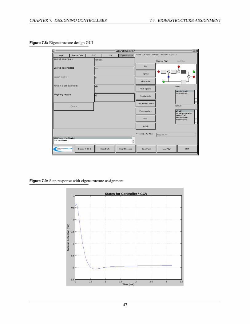
CHAPTER 7. DESIGNING CONTROLLERS 7.4. EIGENSTRUCTURE ASSIGNMENT

Figure 7.8: Eigenstructure design GUI

Figure 7.9: Step response with eigenstructure assignment

States for Controller * CCV

0 0.5 1 1.5 2 2.5 3 3.5-2.5

-2

-1.5

-1

-0.5

0

0.5

1

flap

ero

n d

efle

ctio

n (

rad

)

Time (sec)

47

7.4. EIGENSTRUCTURE ASSIGNMENT CHAPTER 7. DESIGNING CONTROLLERS

48

CHAPTER 8

IMPLEMENTING CONTROLLERS

This chapter shows how to design implement controllers in the nonlinear simulation.

8.1 A General Interface

The function AircraftControl.m provides a general interface that can be used to structure your control system.The following listing shows the entry point for AircraftControl.m.

Listing 8.1: Top of Function AircraftControl.m

function y = AircraftControl( action, d )

persistent s

switch actioncase ’initialize’

s = Initialize( d );case ’update’

[y,s] = Update( s, d );end

AircraftControl.m Here, s is used for global memory. Notice that s is always returned from the internal functions. dis passed to the function to initialize it. y is the output of the controller and s is the updated memory.

This version of AircraftControl just sends commands open loop to the aircraft. The initialization function isshown below.

Listing 8.2: Initialization Function AircraftControl.m

function s = Initialize( d )

s.actuatorName = d.actuatorName;s.control = d.control;

switch d.actuatorNamecase ’elevator’

s.cDS.dT = 0.5;s.cDS.magnitude = 2;s.cDS.init = d.control.elevator;

case ’throttle’s.cDS.dT = 3;

s.cDS.magnitude = 0.1;s.cDS.init = d.control.throttle;

49

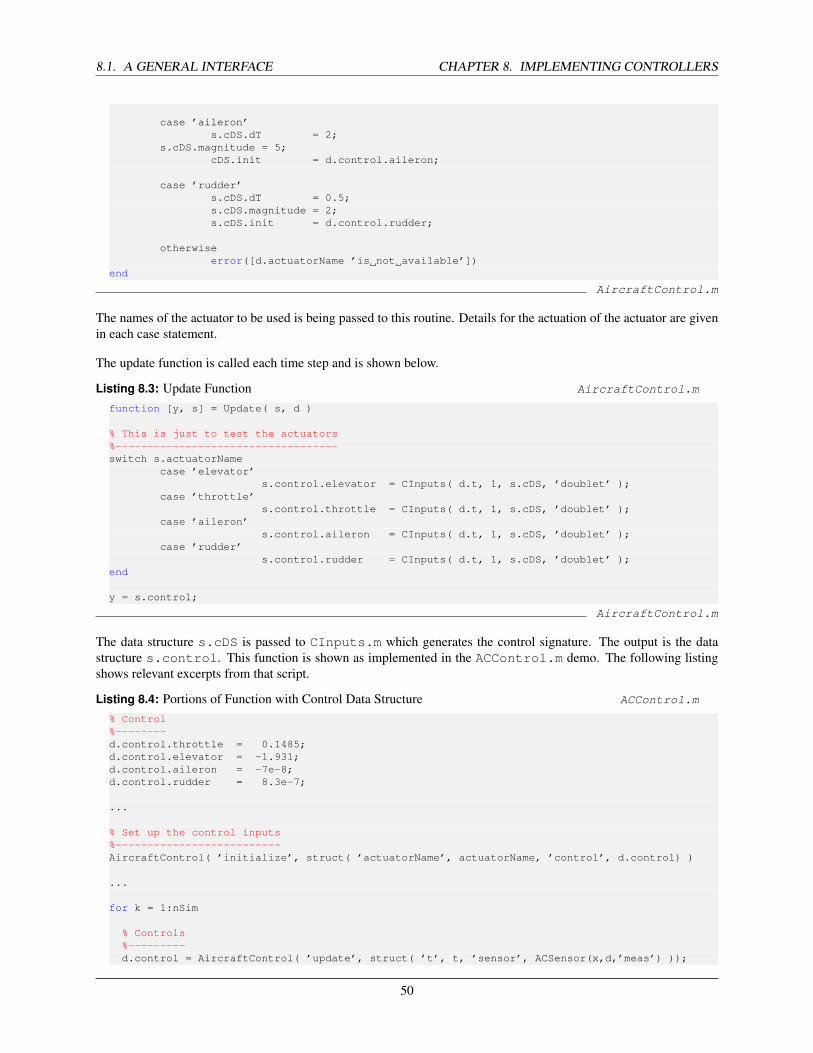
8.1. A GENERAL INTERFACE CHAPTER 8. IMPLEMENTING CONTROLLERS

case ’aileron’s.cDS.dT = 2;

s.cDS.magnitude = 5;cDS.init = d.control.aileron;

case ’rudder’s.cDS.dT = 0.5;s.cDS.magnitude = 2;s.cDS.init = d.control.rudder;

otherwiseerror([d.actuatorName ’is not available’])

end

AircraftControl.m

The names of the actuator to be used is being passed to this routine. Details for the actuation of the actuator are givenin each case statement.

The update function is called each time step and is shown below.

Listing 8.3: Update Function AircraftControl.m

function [y, s] = Update( s, d )

% This is just to test the actuators%-----------------------------------switch s.actuatorName

case ’elevator’s.control.elevator = CInputs( d.t, 1, s.cDS, ’doublet’ );

case ’throttle’s.control.throttle = CInputs( d.t, 1, s.cDS, ’doublet’ );

case ’aileron’s.control.aileron = CInputs( d.t, 1, s.cDS, ’doublet’ );

case ’rudder’s.control.rudder = CInputs( d.t, 1, s.cDS, ’doublet’ );

end

y = s.control;

AircraftControl.m

The data structure s.cDS is passed to CInputs.m which generates the control signature. The output is the datastructure s.control. This function is shown as implemented in the ACControl.m demo. The following listingshows relevant excerpts from that script.

Listing 8.4: Portions of Function with Control Data Structure ACControl.m

% Control%--------d.control.throttle = 0.1485;d.control.elevator = -1.931;d.control.aileron = -7e-8;d.control.rudder = 8.3e-7;

...

% Set up the control inputs%--------------------------AircraftControl( ’initialize’, struct( ’actuatorName’, actuatorName, ’control’, d.control) )

...

for k = 1:nSim

% Controls%---------d.control = AircraftControl( ’update’, struct( ’t’, t, ’sensor’, ACSensor(x,d,’meas’) ));

50

CHAPTER 8. IMPLEMENTING CONTROLLERS 8.2. CLOSED-LOOP CONTROL

ACControl.m

8.2 Closed-Loop Control

8.2.1 Introduction

The function AircraftControl.m can be easily modied to do closed loop control. This example is based on [Ref.C-1] Example 4.5-1, a pitch rate control augmentation system. Note that in the reference the authors implement thepitch augmentation system as an analog system.

There are four parts to this problem:

• Sensor input

• Actuator Model

• Control law

• Pilot input

• Control implementation

In this case we are using the elevator as the actuator. Our inputs are the pitch rate and angle of attack.

Our new control function is called AircraftControlCAS.m. The demo is F16CAS.m. The control design scriptis CASDesign.m.

8.2.2 Sensor Input

The sensors are available from the function ACSensor.m. You will use sensor outputs 5, alpha or angle-of-attack,and 3, q or pitch rate. This sensor model does not include any dynamics.

8.2.3 Actuator Model

The new actuator model is in F16Actuator.m shown in the following listing. Each actuator is modeled as a simplelag. dX is the derivative vector and the control output is now the state x which is the ltered control input.

Listing 8.5: The F16 Actuator Function F16Actuator.m

function [dX, control] = F16Actuator( x, control, d )dX = [...

(control.throttle - x(1))/d.throttleLag;...(control.elevator - x(2))/d.elevatorLag;...(control.aileron - x(3))/d.aileronLag;...(control.rudder - x(4))/d.rudderLag];

control.throttle = x(1);control.elevator = x(2);control.aileron = x(3);control.rudder = x(4);

F16Actuator.m

51

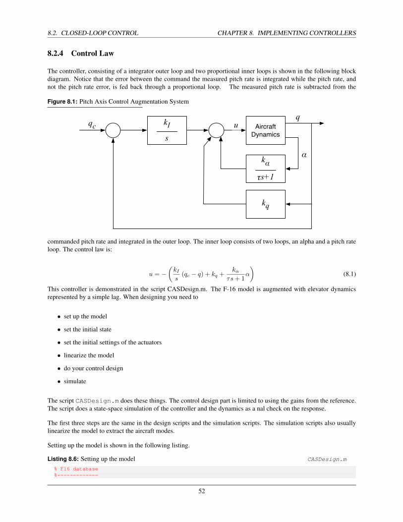
8.2. CLOSED-LOOP CONTROL CHAPTER 8. IMPLEMENTING CONTROLLERS

8.2.4 Control Law

The controller, consisting of a integrator outer loop and two proportional inner loops is shown in the following blockdiagram. Notice that the error between the command the measured pitch rate is integrated while the pitch rate, andnot the pitch rate error, is fed back through a proportional loop. The measured pitch rate is subtracted from the

Figure 8.1: Pitch Axis Control Augmentation System

kI

s

qc AircraftDynamics

kq

kα

τs+1

uq

α

commanded pitch rate and integrated in the outer loop. The inner loop consists of two loops, an alpha and a pitch rateloop. The control law is:

u = −(kIs

(qc − q) + kq +kα

τs+ 1α

)(8.1)

This controller is demonstrated in the script CASDesign.m. The F-16 model is augmented with elevator dynamicsrepresented by a simple lag. When designing you need to

• set up the model

• set the initial state

• set the initial settings of the actuators

• linearize the model

• do your control design

• simulate

The script CASDesign.m does these things. The control design part is limited to using the gains from the reference.The script does a state-space simulation of the controller and the dynamics as a nal check on the response.

The first three steps are the same in the design scripts and the simulation scripts. The simulation scripts also usuallylinearize the model to extract the aircraft modes.

Setting up the model is shown in the following listing.

Listing 8.6: Setting up the model CASDesign.m

% F16 database%-------------

52

CHAPTER 8. IMPLEMENTING CONTROLLERS 8.2. CLOSED-LOOP CONTROL

d = ACBuild(’F16’);d.theta0 = 0;d.wPlanet = [0;0;0];d.actuator.name = ’F16Actuator’;d.aero.name = ’ACAero’;d.engine.name = ’ACEngine’;d.rotor.name = [];d.sensor.name = ’ACSensor’;d.disturb.name = [];% Load the standard atmosphere%-----------------------------d.atmData = load(’AtmData’);d.atmUnits = ’eng’;

% Actuator dynamics%------------------d.actuator.throttleLag = 4.9505e-02;d.actuator.elevatorLag = 4.9505e-02;d.actuator.aileronLag = 4.9505e-02;d.actuator.rudderLag = 4.9505e-02;

CASDesign.m

The data structure entries with the .name fields are the names of the plugin functions, such as the F16Actuatordescribed above. If there is no plugin you enter []. The initial state is loaded as shown in the following listing.

Listing 8.7: Initializing the State CASDesign.m

% Control settings%-----------------d.control.throttle = 0.1385;d.control.elevator = -0.7588;d.control.aileron = -1.2e-7;d.control.rudder = 6.2e-7;

% Initial state vector Corresponding to Nominal in% Table 3.4-3 p. 139 of the reference%-------------------------------------------------altitude = 100;alpha = 0.03691;beta = -4.0e-9;theta = 0.03991;vT = 502;v = VTToVB( vT, alpha, beta );

cG = [0.35;0;0];

r = [2.092565616797901e+07+altitude;0;0];

eulInit = [0;theta;0.00];

q = QECI( r, eulInit );w = [0;0;0];

wR = 160;engine = ACEngEq( d, v, r ); % Engine statemass = 1/1.57e-3;inertia = [9497;55814;63100;0;-982;0];actuator = [0;0;0;0];sensor = [];flex = [];disturb = [];

% Initial time and state%-----------------------x = acstate( r, q, w, v, wR, mass, inertia, cG, engine, actuator, sensor, flex, disturb );

CASDesign.m

53

8.2. CLOSED-LOOP CONTROL CHAPTER 8. IMPLEMENTING CONTROLLERS

We only want to work with the longitudinal dynamics for q and alpha. Extracting those state space matrices isshown in the following listing.

Listing 8.8: Extracting Longitudinal Dynamics CASDesign.m

% Generate the state space model%-------------------------------stateName.actuator = {’Throttle Lag’, ’Elevator Lag’, ’Aileron Lag’, ’Rudder Lag’};d = ACInit( x, d, stateName );g = AC( x, 0, 0, d, ’linalpha’);aC = get( g, ’a’ );cC = get( g, ’c’ );bC = get( g, ’b’ );

kLon = [10 11 5 8 26];kLonAQ = [11 8 26];kAlphaSensor = 5;kQSensor = 3;kElevator = 2;

disp(’The state space matrices for just alpha and q’)a = aC(kLonAQ,kLonAQ)b = bC(kLonAQ,kElevator);c = cC(kAlphaSensor,kLonAQ); % alpha only

disp(’The plant eigenvalues’)eig(a)

CASDesign.m

The printed results of the state space matrices and plant eigenvalues are shown below.

The state space matrices for just alpha and qa =

-1.01671203478116 0.905172891717086 -0.0022528435863352-1.20309885574413 -1.26467603375 -0.1800126

0 0 -20.1999798The plant eigenvaluesans =

-1.14069403426558 + 1.03616646060335i-1.14069403426558 - 1.03616646060335i

-20.1999798

Next, the script constructs a closed-loop system. It first constructs the inner loop by applying a first order integralfeedback controller for alpha. It then constructs the outer loop by feeding back both alpha and q to perform pitchrate tracking.

Listing 8.9: Constructing Closed-Loop System CASDesign.m

% First design the inner loop%----------------------------kAlpha = -0.08; % Notice this sign!tauAlpha = 0.1;aAlpha = -1/tauAlpha;bAlpha = 1/tauAlpha;cAlpha = kAlpha;dAlpha = 0;

% Test it in continuous mode%---------------------------aCL = CLoopS( a, b, c, aAlpha, bAlpha, cAlpha, dAlpha ); % This applies negative feedback

disp(’Closed loop eigenvalues for the inner loop’)eig(aCL)

% Now add the outer loop%-----------------------

54

CHAPTER 8. IMPLEMENTING CONTROLLERS 8.2. CLOSED-LOOP CONTROL

c = cC([kAlphaSensor kQSensor],kLonAQ);kI = 1.5;kQ = -0.5;aCAS = [-1/tauAlpha 0;0 0];bCAS = [1/tauAlpha 0;0 -1];cCAS = [kAlpha kI];dCAS = [0 kQ];

% Test it in continuous mode%---------------------------aCL = CLoopS( a, b, c, aCAS, bCAS, cCAS, dCAS ); % This applies negative feedback

disp(’Closed loop eigenvalues for the inner and outer loops’)eig(aCL)

CASDesign.m

The script does not actually perform a design, it simply uses the gains provided in the reference and checkes theeigenvalues. The printed results of the eigenvalues of the inner and outer loops are:

Closed loop eigenvalues for the inner loopans =

-20.1698093439904-10.1598957054063-1.0758314095672 + 1.39018853926588i-1.0758314095672 - 1.39018853926588i

Closed loop eigenvalues for the inner and outer loopsans =

-13.2616892668476-10.8793554469357-0.85305233171349-3.74363541151719 + 3.37917509890488i-3.74363541151719 - 3.37917509890488i

Finally, the discrete-time system is simulated from zero initial conditions to track a step input of the pitch rae signal.The statespace simulation code is shown below.

Listing 8.10: Constructing Closed-Loop System CASDesign.m

dT = 0.1; % 10 Hz controller works well

[a, b] = C2DZOH( a, b, dT );[aCAS, bCAS] = C2DZOH( aCAS, bCAS, dT );

nSim = 100;

xPlot = zeros(1,nSim);

qC = 1.0;xCAS = [0;0];x = [0;0;0];y = [0;0];

for k = 1:nSim

xPlot(k) = y(2);

y = c*x;

xCAS = aCAS*xCAS + bCAS*[y(1);y(2) - qC];yCAS = -(cCAS*xCAS + dCAS*y);

x = a*x + b*yCAS;

end

t = (0:(nSim-1))*dT;

55

8.3. PILOT INPUT CHAPTER 8. IMPLEMENTING CONTROLLERS

Plot2D( t, xPlot, ’Time (sec)’, ’Q’ );

CASDesign.m

The plot produced from the simulation is shown in Figure 8.2.

Figure 8.2: Pitch Rate Tracking Step Response

Q

0 1 2 3 4 5 6 7 8 9 100

0.1

0.2

0.3

0.4

0.5

0.6

0.7

0.8

0.9

1

Q

Time (sec)

8.3 Pilot Input

Pilot input can be done in two ways. One is just to pass the desired input into your control function. The second is tocustomize the HUD. In this example, we need a pitch rate input which is not an available output on the standard HUD.We would like the pilot to be able to select a pitch rate and then command the aircraft. As an illustrative example, thepilot input can be read in using the following code, which is used in the F16CAS demo.

Listing 8.11: Initializing the controller gains in F16CAS F16CAS.m

% Pitch rate input%-----------------pilotPitchRateInput = struct( ’enter’, hUDOutput.pushbutton1, ’value’, hHUD.control.text1 );

% Controls%---------d.control = AircraftControlCAS( ’update’, struct( ’t’, t, ’sensor’, ACSensor( x, d, ’meas’ ),

’pilotPitchRateInput’, pilotPitchRateInput ) );

F16CAS.m

8.4 Control Implementation

The controller described above is implemented in AircraftControlCAS. As with the previous example there aretwo parts, the initialization and the update. The initialization is shown in the following listing.

56

CHAPTER 8. IMPLEMENTING CONTROLLERS 8.4. CONTROL IMPLEMENTATION

Listing 8.12: Initializing the controller gains AircraftControlCAS.m

function s = Initialize( d )

kI = 1.5;kQ = -0.5;kAlpha = -0.08; % Notice this sign!tauAlpha = 0.1;s.aCAS = [-1/tauAlpha 0;0 0];s.bCAS = [1/tauAlpha 0;0 -1];s.cCAS = [kAlpha kI];s.dCAS = [0 kQ];s.xCAS = [0;0];

[s.aCAS, s.bCAS] = C2DZOH( s.aCAS, s.bCAS, d.dT );s.control = d.control; % Nominal settingss.pilotPitchRateInput = 0;

AircraftControlCAS.m

The update portion is shown below.

Listing 8.13: Updating the controller AircraftControlCAS.m

function [y, s] = Update( s, d )

% Pilot input%------------if( d.pilotPitchRateInput.enter )

s.pilotPitchRateInput = d.pilotPitchRateInput.value;disp(sprintf(’New pitch rate input %12.4f’, s.pilotPitchRateInput))

end

% Input%------input = [d.sensor.alpha; d.sensor.q];

% Control implementation%-----------------------yCAS = -(s.cCAS*s.xCAS + s.dCAS*input);s.xCAS = s.aCAS*s.xCAS + s.bCAS*[input(1);input(2) - s.pilotPitchRateInput];

% Output%-------s.control.elevator = yCAS;y = s.control;

AircraftControlCAS.m

The results are shown in the following plots. A ±1 deg/sec pitch rate doublet is commanded using the rst but- ton onthe HUD. This corresponds to 0.017 rad/s, which is what we see in the plots. You may need to push the button a coupleof times. The call to disp in the above listing prints into the command window to let you know that the commandwent through.

The HUD is shown in Figure 8.3 on the next page. The value of the desired pitch rate in deg/s (in this case “1”) isentered into the text field next to “Button 1” before the button is pushed. In this example, we enter a +1, then a −1,then 0.

The pitch rate response in shown in Figure 8.4 on the following page, in the figure on the left. An initial negative pitchrate occurs to stabilize the aircraft from its slightly off-trim initial condition. Next the doublet is entered and trackedwell. The figure on the right shows the elevator response.

57

8.4. CONTROL IMPLEMENTATION CHAPTER 8. IMPLEMENTING CONTROLLERS

Figure 8.3: HUD Display for F16CAS Demo

Figure 8.4: Pitch Rate Response for F16CAS Demo

Rate (rad/sec)

0 2 4 6 8 10 12 14 16 18 20−0.05

−0.04

−0.03

−0.02

−0.01

0

0.01

0.02

Rat

e (r

ad/s

ec)

Time (sec)

omegaxomegayomegaz

Elevator

0 2 4 6 8 10 12 14 16 18 20−2

−1.8

−1.6

−1.4

−1.2

−1

−0.8

−0.6

−0.4

−0.2

0

Ele

vato

r

Time (sec)

58

CHAPTER 9

PERFORMANCE ANALYSIS

This chapter gives an overview of the tools for analyzing aircraft performance.

9.1 Concorde Properties

The ConcordeProperties function outputs a range of properties for the Concorde.

[d, def] = ConcordeProperties( machNo )

By just typing ConcordeProperties you can generate the following plots:

Figure 9.1: Concorde Properties vs. Mach No.

K1 and K2

1 1.1 1.2 1.3 1.4 1.5 1.6 1.7 1.8 1.9 20

0.05

0.1

0.15

0.2

0.25

0.3

0.35

0.4

K

Mach No

K1K2

(a) Drag Polar Coefficients

Olympus 593

1 1.1 1.2 1.3 1.4 1.5 1.6 1.7 1.8 1.9 23

3.1

3.2

3.3

3.4

3.5x 10

−5

SF

C

1 1.1 1.2 1.3 1.4 1.5 1.6 1.7 1.8 1.9 20.8

1

1.2

1.4

1.6

1.8

2x 10

6

F/d

elta

Mach No

(b) Specific Fuel Consumption (kg/N/s) and Thrust over Pressure Ratio(N)

The function also outputs the following data:

massDry Dry mass kg or lbmmassFuel Fuel mass kg or lbmmassDesign Design point for calculations kg or lbm

59

9.2. BREGUET RANGE EQUATION CHAPTER 9. PERFORMANCE ANALYSIS

sFC Specific fuel consumption kg/N/sec or lbm/lbf/seccL Lift coefficientcD Drag coefficientk1 Drag polar coefficient 1k2 Drag polar coefficient 2wingArea Wing area mˆ2 or ftˆ2wingLoading Wing loading N/mˆ2 or lbf/mˆ2name NamecLCoeff Lift coefficientcLMax Maximum lift coefficientfOverDelta Force over P/P0 N or lbf

The lift and drag properties of the Concorde can be obtained using the ConcordeLD function. It is invoked asfollows:

[cL, cD, k1, k2] = ConcordeLD( machNo );

where the input is Mach number. The function is valid for a Mach range of 1-2. Typing ConcordeLD produces thefollowing plot:

Figure 9.2: Concorde Lift and Drag Properties vs. Mach No.

Concorde Lift and Drag Coeff

0 0.2 0.4 0.6 0.8 1 1.2 1.4 1.6 1.8 20.2

0.3

0.4

K2

0 0.2 0.4 0.6 0.8 1 1.2 1.4 1.6 1.8 20.005

0.01

0.015

K1

0 0.2 0.4 0.6 0.8 1 1.2 1.4 1.6 1.8 20.1

0.2

0.3

0.4

cL

0 0.2 0.4 0.6 0.8 1 1.2 1.4 1.6 1.8 20.01

0.02

0.03

cD

M

The values k1 and k2 are the drag polars, which relate the lift and drag coefficients according to the followingequation:

CD = k1 + k2C2L

9.2 Breguet Range Equation

BreguetRangeEquation generates the Breguet range. The usage is:

>> range = BreguetRangeEquation( d, velocity, altitude )

where d is the data structure generated from ConcordeProperties. To get the demo, just type BreguetRangeEquationand the following figure is generated.

60

CHAPTER 9. PERFORMANCE ANALYSIS 9.3. RATE OF CLIMB

Figure 9.3: Breguet Range

Concorde Range

250 300 350 400 450 500 550 6006000

6500

7000

7500

8000

Ran

ge (

km)

250 300 350 400 450 500 550 6001

1.2

1.4

1.6

1.8

2

Mac

h N

o

Velocity (m/s)

9.3 Rate of Climb

The rate of climb and acceleration can be computed using:

>> [rateOfClimb, accel] = RateOfClimb( d, velocity, altitude )

where d is the data structure generated from ConcordeProperties. Type the function name with no inputs andno outputs to see a plot based on default data.

9.4 Takeoff

The Takeoff function computes the required roll distance and takeoff velocity, given a data structure of the typegenerated by ConcordeProperties, and the takeoff altitude. The usage is:

[sTotal, vLiftoff, def] = Takeoff( d, altitude );

Calling the function name by itself produces the following example:

>> Takeoff;Ground roll = 1753.0 mLiftoff velocity = 78.8 m/s

Field Description UnitscLMax Maximum Lift Coefficient

wingArea Wing area mˆ2 or ftˆ2massTakeoff Mass at takeoff kg or lbm

cDG Drag coefficient on the groundcLG Lift coefficient on the groundcDR Drag coefficient in rotationcLR Lift coefficient in rotation

k2Engine Engine thrust is f = fStatic*(1 + k2Engine*v + k3Engine*vˆ3

61

9.5. STALL VELOCITY CHAPTER 9. PERFORMANCE ANALYSIS

k3Engine See k2EnginemuR Drag decrease due to lift on the ground

fStatic See k2EnginetRotation Rotation time sec

9.5 Stall Velocity

Use VStall to compute the stall velocity.

>> vStall = VStall( d, altitude )

The data structure d must contain the maximum lift coefficient cLMax, the mass massDesign in kg, and the wingarea wingArea in square meters. The built-in demo of the function produces a plot of stall velocity versus altitude.

62

CHAPTER 10

GAS TURBINES

This chapter describes the toolbox functions for the basic design and analysis of gas turbine engines.

10.1 Using the Jet Engine Functions

The jet engine functions let you design gas turbines and analyze their performance. There are three main functions,summarized below.

JetEngineDefinitions.mDenes the data structures used in the other functions. Lists each eld of the input data structures.

JetEngineAnalysis.mThis function does cycle analysis of jet engines.

JetEnginePerformance.mThis function does performance analysis of an existing design including performance at partial throttle settings.

The functions cover a range of engines:

• Ramjet

• Single Spool Turbojet

• Dual Spool Turbojet

• Dual Exhaust Turbofan

• Mixed Exhaust Turbofan

• Turboprop

Any of the turbojet engines can have afterburners. The calling format for the analysis and performance functions are

>> [g, p, d, def] = FUNCTION( p, d );

where p is a data structure with parameters that you plan to vary during the analysis such as compressor pressureratio and burner temperature. d is a data structure with parameters that are xed such as polytropic efciencies.

63

10.2. USING JETENGINEDEFINITIONS CHAPTER 10. GAS TURBINES

10.2 Using JetEngineDefinitions

JetEngineDefinitions gives you denitions of all of the elds in the data structures used by JetEngineAnalysisand JetEnginePerformance. If you type JetEngineDefinitions you will get a list of all engines and theinputs for both the analysis and performance functions. To get just the information for a particular engine combinationtype, for example,

>> JetEngineDefinitions(’analysis’,’ramjet’)

Function: analysis Engine: ramjet

-------------P parameters-------------altitude Altitude m ftmachNo Mach numbertT4 Combustor temperature K R

-------------D parameters-------------analysis ’ideal’ ’real’cPC Air specific heat J/kg-K Btu/lbm-RcPT Air/Fuel specific heat J/kg-K Btu/lbm-ReD Diffuser polytropic efficiencyengine Engine nameetaB Burner efficiencygammaT Burner ratio of specific heatshPR Fuel heating value J/kg Btu/lbmm2 Mach number at the diffuser exitp0OverP9 Inlet/outlet pressure ratiopiB Burner pressure ratiopiDMax Diffuser maximum pressure ratiopiN Nozzle pressure ratiounits ’eng’ or ’mks’

10.3 Using JetEngineAnalysis

Typing just the name JetEngineAnalysis will get you a demo. If you type:

JetEngineAnalysis(’ramjet’)

you will get a ramjet demo. Typing:

JetEngineAnalysis(p,d)

will plot the results. Typing:

[g, d, p, def] = JetEngineAnalysis( p, d );

will put the results in g and echo p and d in the output. def gives you the denitions of p and d.

The following example shows how to analyze a ramjet.

64

CHAPTER 10. GAS TURBINES 10.4. USING JETENGINEPERFORMANCE

Example 10.1 Jet Engine Analysis Demo

1 %---------------------------------------2 % Demo JetEngineAnalysis3 %---------------------------------------4 % Plot specific thrust as a function of5 % mach number and combustion temperature6 %---------------------------------------7

8 p.tT4 = [1600 1900 2200];9 p.altitude = 12000;

10 p.machNo = linspace(0.3,5);11 d.cPC = 1004;12 d.cPT = 1004;13 d.hPR = 42800000;14 d.gammaT = 1.4;15 d.units = ’mks’;16 d.eD = 1.0;17 d.etaB = 1.0;18 d.piB = 1.0;19 d.piDMax = 1.0;20 d.piN = 1.0;21 d.p0OverP9 = 1.0;22 d.analysis = ’real’;23 d.engine = ’ramjet’;24 d.m2 = 0.4;25

26 for k = 1:length(p.machNo)27 g = JetEngineAnalysis(p,d);28 end29

30 Plot2D(p.machNo,g.fOverMDotA,’M’,’F/mDot*Area’,’Jet Engine Analysis’)

31 legend(’1600 K’,’1900 K’,’2200 K’)

Jet Engine Analysis

0 0.5 1 1.5 2 2.5 3 3.5 4 4.5 5100

200

300

400

500

600

700

800

900

F/m

Dot

*Are

a

M

1600 K1900 K2200 K

10.4 Using JetEnginePerformance

Typing just the name JetEnginePerformance will get you a demo. If you type:

JetEnginePerformance(’ramjet’)you will get a ramjet demo. Typing:\begin{codebit}JetEnginePerformance(p,d)

will plot the results. Typing:

[g, d, p, def] = JetEnginePerformance( p, d );

will put the results in g and echo p and d in the output. def gives you the denitions of p and d.

The following listing shows a demo of a single spool turbojet.

65

10.4. USING JETENGINEPERFORMANCE CHAPTER 10. GAS TURBINES

Example 10.2 Jet Engine Performance Demo

1 %--------------------------------2 % Demo JetEnginePerformance3 %--------------------------------4 % Plot thrust as a function of5 % mach number and altitude6 %--------------------------------7 p.altitude = [0 3 6 9 11 12 15]*1e3;8 p.machNo = linspace(0.1,2);9 p.p0OverP9 = 0.955;

10 p.tT4 = 1800;11 p.controlOn = 0;12

13 d.units = ’mks’;14 d.afterburner = 0;15 d.altitude = 12000;16 d.cPC = 1004;17 d.gammaT = 1.3;18 d.cPT = 1239;19 d.tT4 = 1800;20 d.tT7 = 2400;21 d.machNo = 2;22 d.piC = 10;23 d.tauC = 2.0771;24 d.tauT = 0.8155;25 d.piT = 0.3746;26 d.piDMax = 0.95;27 d.piD = 0.8788;28 d.piB = 0.94;29 d.piN = 0.96;30 d.etaB = 0.98;31 d.etaC = 0.8641;32 d.etaM = 0.99;33 d.p0OverP9 = 0.5;34 d.hPR = 42800000;35 d.f = 0.03567;36 d.pT9OverP9 = 11.62;37 d.m0Dot = 50;38 d.piCMax = 12.3;39 d.throttleRatio = 1.2;40 d.engine = ’single spool turbojet’;41

42 g = JetEnginePerformance(p,d);43

44 Plot2D(p.machNo,g.force,’M’,’F (N)’,’JetEngine Performance’)

45 for k = 1:length(p.altitude)46 l{k} = sprintf(’%4.0f km’,p.altitude(k)

/1000);47 end48 legend(l{:},0)

Jet Engine Performance

0 0.2 0.4 0.6 0.8 1 1.2 1.4 1.6 1.8 21

2

3

4

5

6

7

8

9

10

11x 10

4

F (

N)

M

0 km 3 km 6 km 9 km 11 km 12 km 15 km

66

CHAPTER 11

AIRSHIPS

This chapter describes the toolbox functions for developing airship models and simulating their flight. Airships arelighter-than-air vehicles that utilize a buoyancy force to provide static lift. Traditionally, airships have fallen into twocategories: pressurized and rigid. In a pressurized airship, a flexible, lightweight fabric forms the exterior envelope,and the shape of the hull is maintained by a slightly higher internal pressure. With rigid airships, a solid, interior framemaintains the shape. The tools provided in this software package deal only with pressurized airships.

The functionality of the airship code is divided into the following four topics:

• Modeling

• Control

• Analysis

• Simulation

All of the airship functionality is contained in the Airships folder. This folder is organized into four sub-foldersaccording to the above topics. The remainder of this chapter describes the tools available under each category.

11.1 Modeling

An aerodynamic model of an airship may be built using the functions in the Modeling folder. The complete airshipmodel consists of the hull, a single hanging gondola, and four symmetric fins.

The hull is modeled as a double-ellipsoid, with a front semi-major axis a1, a rear semi-major axis a2, and commonradius b. The ratio of the rear ellipsoid to the front ellipsoid, k, is approximately 2 for the classic teardrop shape. Onemay choose the overall length L, diameter D, and ratio k, then use the following function to view the geometry:

>> DrawAirship( L, D, k );

The surface area and volume of the hull, as well as the ellipsoid axes, may be computed with:

>> [S, V, a1, a2, b] = AirshipGeometry( L, D, ratio );

THe total drag at a particular altitude h and velocity u may be computed using:

>> D = AirshipDrag( h, u, A, Cd );

67

11.1. MODELING CHAPTER 11. AIRSHIPS

where A is the reference area and CD is the drag coefficient.

The aerostatic properties of a pressure airship show that a constant buoyancy force is maintained up to a “pressurealtitude//. The magnitude of the buoyancy force depends upon the volume of the hull and the density of the air at thepressure altitude. The airship should be designed so that the static lift of the buoyancy force can offset the weight ofthe vehicle. The function StructuralMass.m can be used to evaluate the feasibility of a given design with respectto its size and mass. The default inputs can be used to generate a plot by simply calling the function name:

>> StructuralMass

The following plot shows how the mass available for airship structure and systems varies with increasing fabric density,for a range of airship geometries. Each line represents a different value of kSV , which is the ratio of hull surface areato volume.

Figure 11.1: Structural Mass Dependence on Geometry and Fabric Density

0 0.2 0.4 0.6 0.8 1−4

−3

−2

−1

0

1

2

3

4

5x 10

4

fabric density, ρf [kg/m2]

m0

[kg]

kSV

= 0.01

kSV

= 0.03

kSV

= 0.05

kSV

= 0.07

kSV

= 0.09

kSV

= 0.11

Clearly, as the fabric density increases, and as the surface-to-volume ratio increases (increasingly slender airship), themass available for structure and systems decreases. The available mass is much higher for lower altitudes. This pointsto one of the key challenges in high-altitude airship design: the need for ultra-light materials.

Another type of trade-off analysis may be done with respect to the power. The maximum required power for nominaloperation depends upon the drag, cruise velocity, and propeller efficiency. Additional power is likely required for thepayload. A sufficient area of solar cells must be placed on the top of the airship hull in order to provide the requiredpower. This area depends upon the required power, the solar cell efficiency, the global irradiance, and the dailyfraction of sun-exposure. Given these parameters, the function SolarCellCoverage.m can be used to evaluatethe required solar cell coverage for a particular hull geometry. To see a demo:

>> SolarCellCoverage

The following plot shows how the solar cell coverage ratio R varies with different levels of propeller and solar cellefficiencies. R is the ratio of required solar cell area to hull surface area. The required solar cell area is derived fromthe power requirement for extended operation of the turbines at a specified airspeed.

The top set of curves correspond to a maximum airspeed of 40 mph, and the lower set of curves are for 103 mph.These are the expected average and maximum windspeeds an airship would encounter over the U.S. at an altitude of70k ft.

A graphical user interface may be used for conducting the high-level types of trade-offs discussed above. Just type:

>> AirshipDesignGUI

68

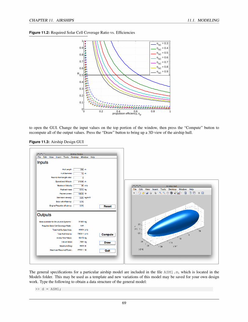
CHAPTER 11. AIRSHIPS 11.1. MODELING

Figure 11.2: Required Solar Cell Coverage Ratio vs. Efficiencies

0 0.2 0.4 0.6 0.8 10

0.1

0.2

0.3

0.4

0.5

0.6

0.7

0.8

0.9

1

propulsion efficiency, ηP

R

η

SC = 0.3

ηSC

= 0.4

ηSC

= 0.5

ηSC

= 0.6

ηSC

= 0.7

ηSC

= 0.8

ηSC

= 0.9

to open the GUI. Change the input values on the top portion of the window, then press the “Compute” button torecompute all of the output values. Press the “Draw” button to bring up a 3D view of the airship hull.

Figure 11.3: Airship Design GUI

The general specifications for a particular airship model are included in the file ASM1.m, which is located in theModels folder. This may be used as a template and new variations of this model may be saved for your own designwork. Type the following to obtain a data structure of the general model:

>> d = ASM1;

69

11.1. MODELING CHAPTER 11. AIRSHIPS

The parameters in d represent the high-level design parameters for the airship configuration. This data structure maybe used to build an approximate aerodynamic model. To build an airship aero model, type:

>> m = BuildAirshipModel( name, xo );

where name is the string name of the airship model file, and xo is the axial displacement of the body-frame origin,measured positive backwards from the nose. The coefficients and moment of inertia included within the aerodynamicmodel depend upon the location of the body-frame. If no inputs are provided, defaults are used (the default modelname is ‘ASM1’).

11.1.1 Baseline Airship Design

This section describes a baseline airship design to provide an illustrative example for new users.

As previously noted, the airship hull is modeled as two half-ellipsoids. A diagram of the the x-z plane cross-section isshown in Figure 11.4. The total length is L = a1+a2 and the maximum diameter isD = 2b. Note that this coordinateframe is aligned with the body frame, but the two frames are not coincident. The body frame is centered at the hull’sCV, while this frame is located at the intersection of the two half-ellipsoids. Each half-ellipsoid is symmetric about

Figure 11.4: Double-Ellipsoid Model of Hull

12

the x-axis, and the rear ellipsoid is longer than the front, resulting in the classic “teardrop” shape.

Attached to the hull are four symmetric tail-fins and a hanging gondola, or empennage. The empennage supportsthe payload as well as two engines with counter-rotating propellers. The size and shape of the hull, and the size andlocation of the fins and gondola are defined in an airship design script in MATLAB. In addition to these geometricproperties, you may also specify the payload mass, fabric density, and maximum altitude. The parameters that may bedefined in the airship design script are summarized in Table 11.1.

Table 11.1: Airship Design Parameters

Parameter Description UnitsL Length of hull mD Maximum diameter of hull mratio Ratio of rear ellipsoid length to front ellipsoid length, a2/a1 > 1 -alt Maximum altitude mmP Payload mass kgrhoF Fabric area density kg/m2

xGonA x location of gondola L.E. -xGonB x location of gondola T.E. -zGon Minimum z location of gondola (g.t. 1) -xFinA x location of fin L.E. -xFinB x location of fin taper -xFinC x location of fin T.E. -

70

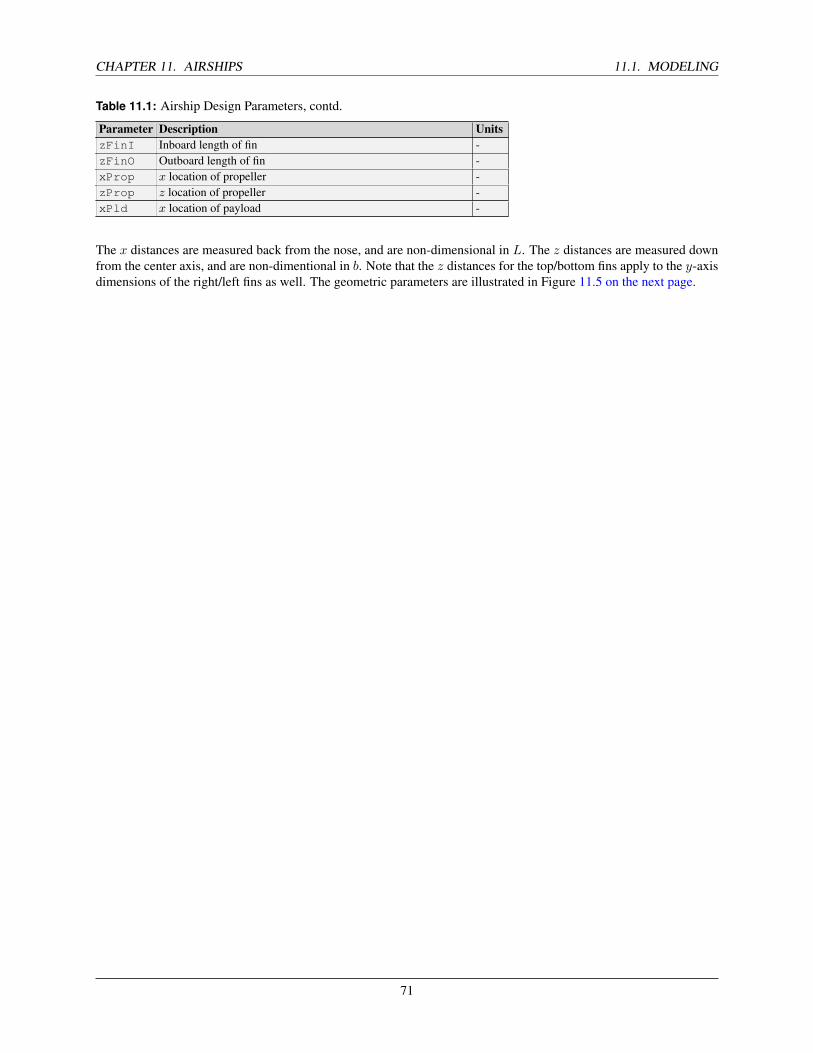
CHAPTER 11. AIRSHIPS 11.1. MODELING

Table 11.1: Airship Design Parameters, contd.

Parameter Description UnitszFinI Inboard length of fin -zFinO Outboard length of fin -xProp x location of propeller -zProp z location of propeller -xPld x location of payload -

The x distances are measured back from the nose, and are non-dimensional in L. The z distances are measured downfrom the center axis, and are non-dimentional in b. Note that the z distances for the top/bottom fins apply to the y-axisdimensions of the right/left fins as well. The geometric parameters are illustrated in Figure 11.5 on the next page.

71

11.1. MODELING CHAPTER 11. AIRSHIPS

Figure 11.5: Airship Geometric Model

x G o n Ax G o n B

x F i n Ax F i n Bx F i n C

z F i n Iz F i n O z G o nx P r o p

z P r o p

An example airship configuration is shown in Figure 11.6. This plot was generated automatically from the functionAirship3DLayout.m by passing in the name of the airship design script. This function can be used to quicklyvisualize any airship design.

Figure 11.6: Example Airship Configuration

−60 −50 −40 −30 −20 −10 0 10 20 30 −100

10

−20

−10

0

10

y [m]x [m]

z[m]

The design parameters for this configuration are summarized in Table 11.2. These values correspond to an airshipgeometry that was designed to meet critical force and energy balance constraints, and the dimensions are similar tothose quoted by other institutions currently developing high-altitude airship prototypes.

Table 11.2: Example Design Parameters

Parameter Value UnitsL 150 mD 50 mratio 1.25 -alt 21,336 mmP 1363 kgrhoF 0.08 kg/m2

72

CHAPTER 11. AIRSHIPS 11.2. CONTROL

Table 11.2: Airship Design Parameters, contd.

Parameter Value UnitsxGonA 0.35 -xGonB 0.45 -zGon 1.20 -xFinA 0.75 -xFinB 0.80 -xFinC 0.95 -zFinI 0.85 -zFinO 1.00 -xProp 0.35 -zProp 1.20 -xPld 0.385 -

11.2 Control

In order to develop a feedback control design for airships, it is instructive to work with a linearized model. Thefunction AirshipLinMod.m may be used to quickly generate a linear model of a particular airship configuration ata chosen flight condition. The function is called as follows:

>> g = AirshipLinMod( m, h, theta, alpha, V );

where m is the aerodynamic model data structure (computed from BuildAirshipModel), h is the altitude inmeters, theta is the pitch angle, alpha is the angle of attack, and V is the wind-relative velocity. The output g is astatespace object containing the continuous time A,B,C,D matrices.

The names of the inputs, outputs, and states of the linear model may always be obtained by typing:

>> get(g,’inputs’)>> get(g,’outputs’)>> get(g,’states’)

and the A,B,C,D matrices may be obtained using:

>> [a,b,c,d] = getabcd( g );

One may wish to break the single linear model into its constituent longitudinal and lateral modes. This may be donewith:

>> [gLat,gLon] = AirshipStatespace( g );

In order to obtain the linearized models, the trim condition must be computed. This is done with the functionAirshipTrim.m. It is called with the same inputs as AirshipLinMod:

>> [T,mu,dElv] = AirshipTrim( d, h, theta, alpha, V );

With the linearized models in hand, you can use the control design techniques of your choice to develop a feedbackcontrol law for the airship at this operating condition.

The outputs are trim thrust T, propeller pitch angle mu, and elevator deflection dElv. This total deflection is to beapplied to both the left and right elevators. The thrust is the total trim thrust. Therefore, with two engines (one on eachside), each engine should produce half of this thrust.

For an example of controlled flight of an airship, you can view and run the function AirshipControlDemo.m. Thisfunction initializes the airship at 21.3 km altitude, with 24 m/s airspeed. A velocity increase of 5 m/s is commanded.A set of pre-designed controllers are loaded and used to form the feedback control loops.

73

11.3. ANALYSIS CHAPTER 11. AIRSHIPS

11.3 Analysis

Several tools are provided to enable immediate analysis of airship data.

• The latitude and longitude of several major U.S. cities may be computed by entering the name of the city

• The wind behavior at a particular day of the year and altitude may be computed for a range of latitudes andlongitudes

• Linear models of a particular airship design may be computed for a range of flight conditions

• The aerodynamic forces and moments of a particular airship design may be computed over a range of flightconditions

• The control settings required for trim flight of a particular airship design may be computed over a range of flightconditions

The following plot was generated by the built-in demo included in WindLatLon.m. It shows the average magnitudeand direction of the wind at 21.3 km altitude in the summer time over a range of latitudes and longitudes. The windstrength varies considerably with latitude, and very little with longitude. This data is generated using an empiricalmodel that was developed by the Naval Research Laboratory.

Figure 11.7: Demo Results from WindLatLon

30 35 40 45 504

5

6

7

8

9

10

11

12

latitude [deg]

|W|[m/s]

long = −120long = −115long = −110long = −105long = −100long = −95long = −90long = −85long = −80long = −75long = −70

30 35 40 45 50−95

−94.5

−94

−93.5

−93

−92.5

−92

−91.5

latitude [deg]

Ψ[deg]

long = −120long = −115long = −110long = −105long = −100long = −95long = −90long = −85long = −80long = −75long = −70

The control settings required for trim flight may be analyzed by calling two functions. First, compute the aerodynamicforces and moments for a variety of flight conditions by using the function GenerateAirshipAeroMats.m. Itwill compute matrices of forces and torques for a range of angles of attack and velocities at a particular altitude. Next,compute the required thrust, propeller pitch angle, and elevator deflection to achieve trim flight at these conditions:

>> data = GenerateAershipAeroMats;>> data = AirshipTrimAnalysis( data );

11.4 Simulation

Airships are simulated within the Aircraft Control Toolbox in the same manner as regular aircraft. The 6 degree offreedom equations of motion for a rigid body are integrated using the standard 4th order Runge-Kutta method. The

74

CHAPTER 11. AIRSHIPS 11.4. SIMULATION

forces and moments due to gravity, aerodynamics, engines/propellers and disturbances are computed at each step. Theeffects of added mass and inertia are also accounted for, with the values of added mass and inertia provided by theaerodynamics function.

The functions used for the full non-linear airship simulation include:

AirshipAero – Compute the aerodynamic force and moment given the current state and flap deflections

AirshipSensor – Return the measured states (angular velocity, linear velocity, angle of attack, sideslip, altitude)

AirshipPropeller – Compute the applied thrust from throttle and propeller pitch commands

These names are provided to the simulation automatically by the BuildAirshipModel.m function. New modelsmay be developed to substitute the originals for new airship designs. The appropriate model names must be includedin the airship model data structure. Once a model has been built, the model names may be easily changed as follows:

>> m.aero.name = ’NewAeroName’;>> m.sensor.name = ’NewSensorName’;>> m.actuator.name = ’NewActuatorName’;>> m.engine.name = ’NewEngineName’;

An interactive demo is provided which allows you to “fly” the airship using a HUD (heads up display) interface. Toinitiate the demo:

>> FlyAirship

75

11.4. SIMULATION CHAPTER 11. AIRSHIPS

76

CHAPTER A

USING DATABASES

This chapter shows you how to use the database and constant functions in the toolboxes. These functions allow youto manage the various constants and parameters used in your projects and ensure that all of your engineers are usingconsistent numbers in their analyses.

A.1 The Constant Database

The constant database gives a substantial selection of useful constants. If you type Constant you will get the GUIin Figure A.1.

Figure A.1: Constant database

The list on the left is a list of all of the constants in the database. You can enter a search string and look for matchesby hitting Find. If you then click one of the selections the GUI looks like it does in the following figure. This functionalways loads its constants from the .mat file ACTConstants.mat

The string field shows the parameter name. Directly below it is the value for the parameter. The value may be anyMATLAB construct. Directly below that is a field for units, then a field for reference information and finally a fieldthat gives a template for the function. You can cut and paste this into any function or script. Searches are insensitive to

77

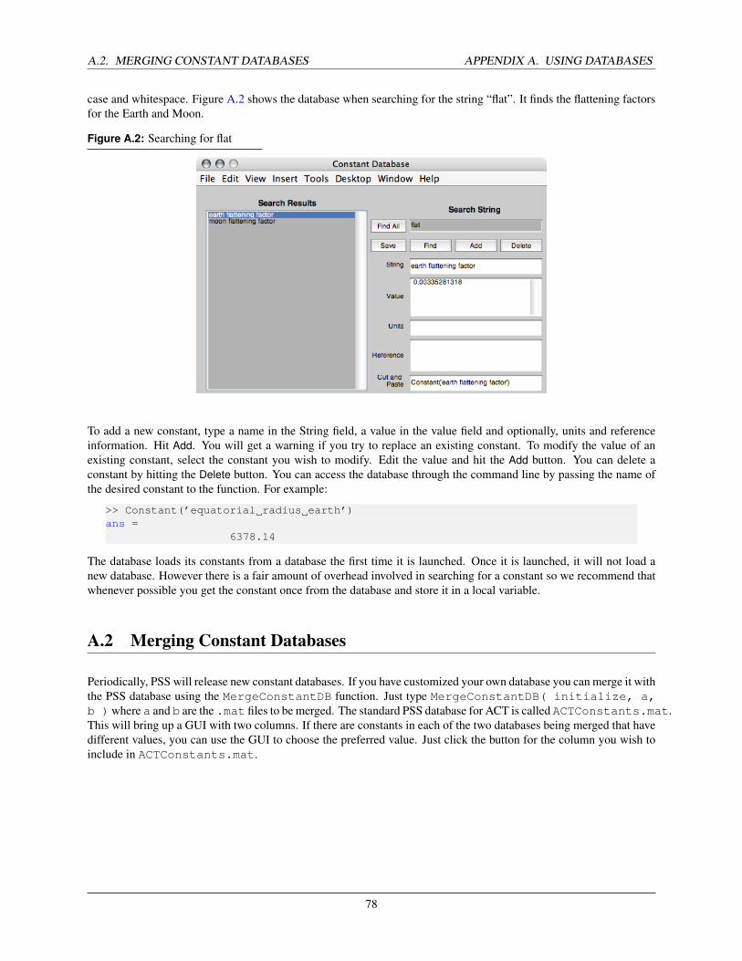
A.2. MERGING CONSTANT DATABASES APPENDIX A. USING DATABASES

case and whitespace. Figure A.2 shows the database when searching for the string “flat”. It finds the flattening factorsfor the Earth and Moon.

Figure A.2: Searching for flat

To add a new constant, type a name in the String field, a value in the value field and optionally, units and referenceinformation. Hit Add. You will get a warning if you try to replace an existing constant. To modify the value of anexisting constant, select the constant you wish to modify. Edit the value and hit the Add button. You can delete aconstant by hitting the Delete button. You can access the database through the command line by passing the name ofthe desired constant to the function. For example:

>> Constant(’equatorial radius earth’)ans =

6378.14

The database loads its constants from a database the first time it is launched. Once it is launched, it will not load anew database. However there is a fair amount of overhead involved in searching for a constant so we recommend thatwhenever possible you get the constant once from the database and store it in a local variable.

A.2 Merging Constant Databases

Periodically, PSS will release new constant databases. If you have customized your own database you can merge it withthe PSS database using the MergeConstantDB function. Just type MergeConstantDB( initialize, a,b )where a and b are the .mat files to be merged. The standard PSS database for ACT is called ACTConstants.mat.This will bring up a GUI with two columns. If there are constants in each of the two databases being merged that havedifferent values, you can use the GUI to choose the preferred value. Just click the button for the column you wish toinclude in ACTConstants.mat.

78

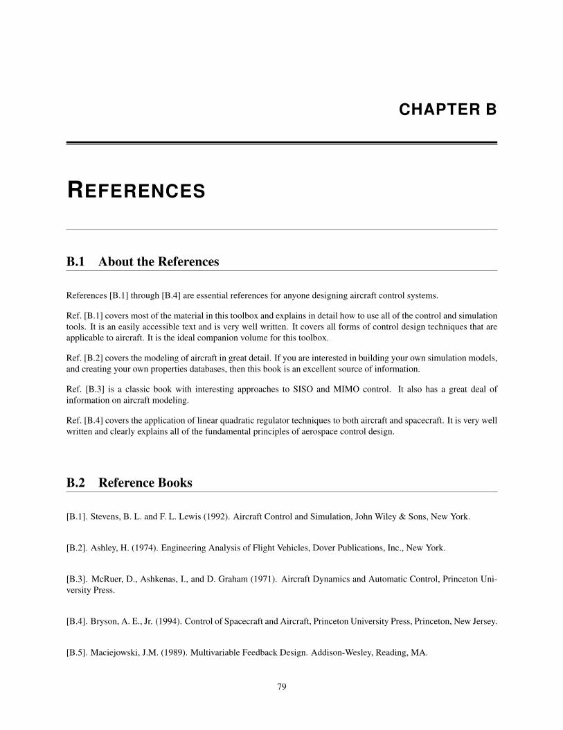
CHAPTER B

REFERENCES

B.1 About the References

References [B.1] through [B.4] are essential references for anyone designing aircraft control systems.

Ref. [B.1] covers most of the material in this toolbox and explains in detail how to use all of the control and simulationtools. It is an easily accessible text and is very well written. It covers all forms of control design techniques that areapplicable to aircraft. It is the ideal companion volume for this toolbox.

Ref. [B.2] covers the modeling of aircraft in great detail. If you are interested in building your own simulation models,and creating your own properties databases, then this book is an excellent source of information.

Ref. [B.3] is a classic book with interesting approaches to SISO and MIMO control. It also has a great deal ofinformation on aircraft modeling.

Ref. [B.4] covers the application of linear quadratic regulator techniques to both aircraft and spacecraft. It is very wellwritten and clearly explains all of the fundamental principles of aerospace control design.

B.2 Reference Books

[B.1]. Stevens, B. L. and F. L. Lewis (1992). Aircraft Control and Simulation, John Wiley & Sons, New York.

[B.2]. Ashley, H. (1974). Engineering Analysis of Flight Vehicles, Dover Publications, Inc., New York.

[B.3]. McRuer, D., Ashkenas, I., and D. Graham (1971). Aircraft Dynamics and Automatic Control, Princeton Uni-versity Press.

[B.4]. Bryson, A. E., Jr. (1994). Control of Spacecraft and Aircraft, Princeton University Press, Princeton, New Jersey.

[B.5]. Maciejowski, J.M. (1989). Multivariable Feedback Design. Addison-Wesley, Reading, MA.

79

B.3. PAPERS APPENDIX B. REFERENCES

[B.6]. Zhou, K., (1998). Essentials of Robust Control. Prentice-Hall, New Jersey.

[B.7]. Dutton, K., S. Thompson, and B. Barraclough. (1997). The Art of Control Engineering. Addison-Wesley,Reading, MA.

[B.8]. Abzug, M. J., and E. E. Larrabee. (1997). Airplane Stability and Control. Cambridge University Press.

[B.9]. Mattingly, J. D. (1996). Elements of Gas Turbine Propulsion. McGraw-Hill.

[B.10]. Nelson, R. C (1998). Flight Stability and Automatic Control. Second Edition, McGraw-Hill.

[B.11]. Gracey, W. (1980). Measurement of Aircraft Speed and Altitude. NASA Reference Publication 1046.

[B.12]. Nahin, P.J. (2000). Dualing Idiots and Other Probability Puzzlers. Princeton University Press.

[B.13]. de Silva, C. W. ().Control Sensors and Actuators. Prentice-Hall, 1989.

[B.14]. Trucco, E. and A. Verri (1998.) Introductory Techniques for 3-D Computer Vision. Prentice-Hall.

[B.15]. Khoury, G. A. and J. D. Gillett, Airship Technology, Cambridge Aerospace Series: 10, 1999.

B.3 Papers

[B.16]. Andry, A. N., Jr., Shapiro, E.Y. and J.C. Chung, “Eigenstructure Assignment for Linear Systems,” IEEE Trans-actions on Aerospace and Electronic Systems, Vol. AES-19, No. 5. September 1983.

[B.17]. Hung, Y. S., and MacFarlane A.G.J. (1982). 11Multivariable Feedback: A Quasi-classical Approach.” LectureNotes in Control and Information Sciences, Vol. 40. Berlin: Springer- Verlag.

[B.18]. Stein, G. and Athans, M. (1987). The LQG/LTR Procedure for Multivariable Feedback Control Design. IEEETransactions on Automatic Control, AC-32(2), 105-114.

[B.19]. Anderson, B.D.O. and Mingori, D.L. (1985). Use of Frequency Dependence in Linear Quadratic ControlProblems to Frequency-Shape Robustness. J. Guidance and Control, 8(3), 397-401.

[B.20]. MacFarlane, A.G.J. and Postlethwaite, I. (1977). The generalized Nyquist stability criterion and multivariableroot loci. Int. J. Control, 25(1), 81-127.

[B.21]. Edmunds, J.M. (1979). Controls system design and analysis using closed-loop Nyquist and Bode arrays. Int.

80

APPENDIX B. REFERENCES B.3. PAPERS

J. Control, 30(5), 773-802.

[B.22]. Doyle, J.C. and Stein, G. (1981). Multivariable Feedback Design: Concepts for a Classical/Modern Synthesis.IEEE Transactions on Automatic Control, AC-26(1), 4-16.

[B.23]. Dorato, P. (1987). A Historical Review of Robust Control. IEEE Control Systems Magazine, 7(2),44-47.

[B.24]. MacFarlane, D.C. and Glover, K. (1989). Robust Control Design Using Normalized Coprime Factor PlantDescriptions. Springer-Verlag, Berlin.

[B.25]. Doyle, J.C. and G.J. Balas (1990). Identification of Flexible Structures for Robust Control. IEEE ControlSystems Magazine, 10(4),51-58.

[B.26]. Fan, M.K.H and Tits A.L. (1988). m-form numerical range and the computation of the structured singularvalue. IEEE Transactions on Automatic Control, AC-33, 284-289.

[B.27]. Safonov, M. and Doyle J.C. (1984). Minimizing conservativeness of robustness singular values. MultivariableControl: New Concepts and Tools (Tzafestas S.G., ed.), Dordrecht: Reidel, 197-207.

[B.28]. Doyle, J.C. (1978). Guaranteed margins for LQG regulators. IEEE Transactions on Automatic Control, AC-23, 756-757.

[B.29]. Horowitz, I. and Sidi, M. (1980). Practical design of feedback systems with uncertain multivariable plants.Int. J. Systems Sci., 11(7), 851-875.

[B.30]. Horowitz, I. (1979). Quantitative synthesis of uncertain multiple input-output feedback system. Int. J. Control,30(1), 81-106.

[B.31]. Park, M.S., Chait, Y. and Steinbuch, M. (1994). A New Approach to Multivariable Quantitative FeedbackTheory: Theoretical and Experimental Results. ASME J. DSMC.

[B.32]. Hamel, P.G. (1994). Aerospace vehicle modeling requirements for high bandwidth flight control. AerospaceVehicle Dynamics and Control, Oxford University Press, Oxford, 1-32.

[B.33]. Hyde, R.A. and Glover, K. (1994). Flight controller design using multivariable loop shaping. AerospaceVehicle Dynamics and Control, Oxford University Press, Oxford, 81-102.

[B.34]. Carr, S.A. and Grimble, M.J. (1994). Comparison of LQG, H and classical designs for the pitch rate controlof an unstable military aircraft. Aerospace Vehicle Dynamics and Control, Oxford University Press, Oxford, 103-124.

[B.35]. Gribble, J.J., et al. (1994). Helicopter flight control design: multivariable methods and design issues.Aerospace Vehicle Dynamics and Control, Oxford University Press, Oxford, 199-224.

81

B.4. WEBSITES APPENDIX B. REFERENCES

[B.36]. Mueller, J. B, Applications of Linear-Parameter Varying Control Techniques to the F/A-18 Systems ResearchAircraft, Master’s thesis, University of Minnesota, July 2000.

[B.37]. Andry, A. N., Shapiro, E. Y. and J. C. Chung, Eigenstructure Assignment for Linear Systems, IEEE Transac-tions on Aerospace and Electronic Systems, Vol. AES-19, No. 5., September 1983, pp.711-729.

[B.38]. Lee, H. P., Jr., Yousseff, H.M. and R.P. Habek, Application of Eigenstructure Assignment to the Design ofSTOVL Flight Control Systems, AIAA 88-4140-CP.

[B.39]. A.E. Hedin, E.L. Fleming, A.H. Manson, F.J. Scmidlin, S.K. Avery, R.R. Clark, S.J. Franke, G.J. Fraser, T.Tsunda, F. Vial and R.A. Vincent, Emperical Wind Model for the Upper, Middle, and Lower Atmosphere, J. Atmos.Terr. Phys., 58, 1421-1447, 1996.

[B.40]. Rehmet, Dr. Michael A., B. Krplin, F. Epperlein, R. Kornmann, R. Shcubert, Recent Developments on HighAltitude Platforms, http://www.isd.uni-stuttgart.de/lotte/halp/paper/paper.htm

B.4 Websites

[B.41]. http://uap-www.nrl.navy.mil/models web/hwm/hwm home.htm.

[B.42]. http://www.lockheedmartin.com/akron/protech/aeroweb/aerostat/haaphase1pr.htm

[B.43]. http://www.nidsci.org/articles/blimps.html

[B.44]. http://www.acq.osd.mil/bmdo/barbb/haaactd.htm

[B.45]. http://www.lindstrand.co.uk/hale.htm

82