-1 of 33-

Introduction Embedded systems

Continue pervasive expansion into Vast variety of electronic systems and products

Aircraft and automobiles → games and medical equipment

Have difficulty identifying any products Not incorporating embedded processor FPGA or CPLD

In one form or another Different kinds of computing

We identify three basic kinds of component We embed into our systems

Leaving FPGA and CPLD aside for moment

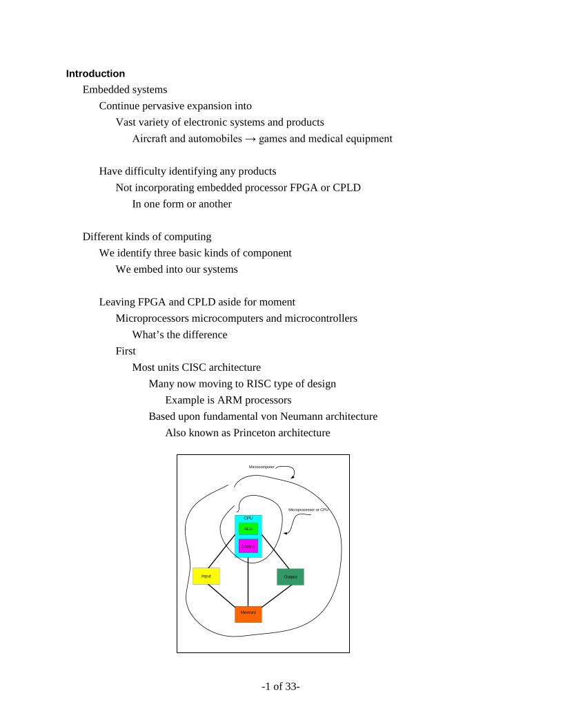
Microprocessors microcomputers and microcontrollers What’s the difference

First Most units CISC architecture

Many now moving to RISC type of design Example is ARM processors

Based upon fundamental von Neumann architecture Also known as Princeton architecture

CPU

ALU

Control

Memory

Input Output

Microprocessor or CPU

Microcomputer

-2 of 33-

Microprocessor Integrated implementation of central processing unit – CPU

Given in above diagram Thus often simply referred to as CPU Microprocessors will differ in

Complexity Power Cost One may also find differences in

Number of registers Overall control Bus structure

Increasingly Aiken or Harvard architecture Becoming mixed in

In addition RISC features being utilized as well Microprocessors range from devices with

Few thousand transistors Cost of a dollar or less

Units with 5-10 million transistors Cost several thousand dollars

To implement complete computer

Must still include Input / output subsystems Memory

Will examine each of these in detail In context of embedded system

Such components connected via system bus

Microcomputer Complete computer

Implemented using microprocessor Typically constructed utilizing

Numerous integrated circuits Once again complexity varies

-3 of 33-

Simple microcomputers Can be implemented on single chip These will have limited

Onboard memory Simple I/O system

Microcontroller

Includes Microprocessor I/O subsystems

Typically these include such things as Timers Serial communications channels Analog to digital conversion Digital to analog conversion DMA

Memory subsystem May or may not be included

Embedded Systems an Overview An embedded system microcomputer system

Comprising hardware and software Designed and optimized

To solve specific problem very efficiently Typically continually

Interacts with environment Monitor and control some process

Term embedded system refers to fact Microcomputer system

Enclosed or embedded In larger system

Typical person May interact with 10-20 embedded systems

Around home each day

-4 of 33-

Single contemporary automobile May contain as many as 100 embedded microprocessors and microcontrollers

Engine ignition Transmission shifting Power steering Antilock braking Security Entertainment

Typically consider two types of embedded system

Reactive Time based

Reactive

Reactive embedded system Typically event driven

Implies asynchronous behaviour Continually interacting with its environment Comprises two sets of tasks

Foreground Background

Foreground component Interact with user Initiated by

Interrupt Real-time constraint

Background component Remainder

Not interrupt driven Once started

Typically run to completion Can be interrupted by foreground task

-5 of 33-

Timebased Considered synchronous Systems whose behaviour controlled by time Tasks execute according to some schedule

Time Constraints Many embedded systems

Considered to be real time systems System with real-time constraint

Can be either Reactive Time based

Real time system

Must respond within constrained time interval To external or internal events

Response is execution of task associated with event

Such systems classed into two general categories Soft real time system

If time constraint not met Performance degraded

Hard real time system If time constraint not met

System considered to have failed Failure may be considered to be catastrophic

When operating system used in embedded microcomputer

Typically is real time operating system Real time operating (RTOS)

Designed and optimized To handle strict time constraints

Associated with events in real time context

-6 of 33-

Architecture

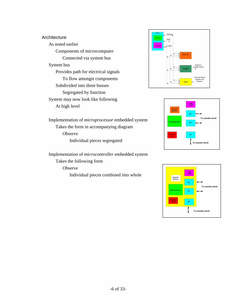
As noted earlier Components of microcomputer

Connected via system bus System bus

Provides path for electrical signals To flow amongst components

Subdivided into three busses Segregated by function

System may now look like following At high level

Implementation of microprocessor embedded system

Takes the form in accompanying diagram Observe

Individual pieces segregated

Implementation of microcontroller embedded system Takes the following form

Observe Individual pieces combined into whole

CPU

ALU

Control

Memory

Output

Input

Address

Data

Control

Signal toOutside World

External WorldSignals into

System

Microprocessor I/O

Real-timeClock

I/O

To outside world

I/O

DataStore

To outside world

ProgramMemory

Microprocessor

To outside world

I/O

To outside world

ProgramMemory

Real-timeClock I/O

I/O

DataStore

-7 of 33-

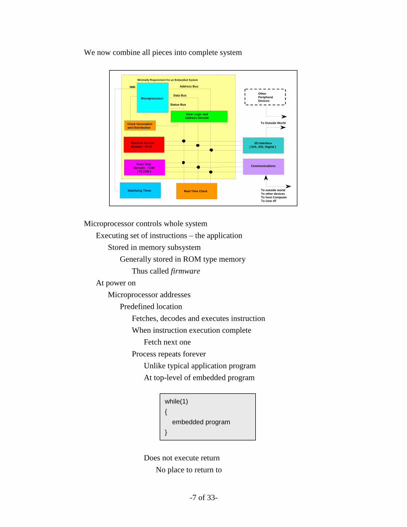
We now combine all pieces into complete system

Microprocessor controls whole system

Executing set of instructions – the application Stored in memory subsystem

Generally stored in ROM type memory Thus called firmware

At power on Microprocessor addresses

Predefined location Fetches, decodes and executes instruction When instruction execution complete

Fetch next one Process repeats forever

Unlike typical application program At top-level of embedded program

Does not execute return

No place to return to

while(1) { embedded program }

Microprocessor

Address Bus

Data Bus

Status Bus

Glue Logic andAddress Decode

Clock Generationand Distribution

Real Time Clock

Random AccessMemory - RAM

Read OnlyMemory - ROM

( FLASH )

Minimally Requirement for an Embedded System

I/O Interface( D/A, A/D, Digital )

Communications

OtherPeripheralDevices

To Outside World

To outside worldTo other devicesTo host ComputerTo User I/F

Watchdog Timer

NMI

-8 of 33-

Specific set of instructions for microprocessor Called instruction set Design first -> architecture

Called ISA or Instruction Set Architecture Instructions or control flow

Sequential Branch Loop Function call

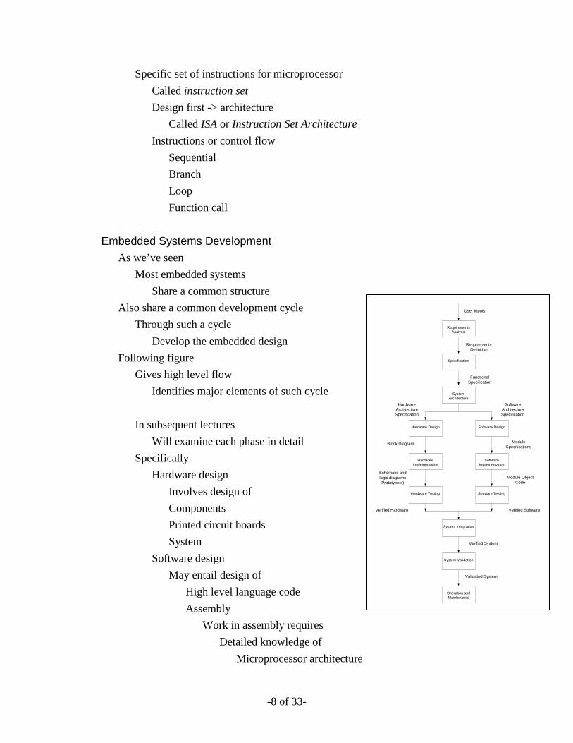
Embedded Systems Development As we’ve seen

Most embedded systems Share a common structure

Also share a common development cycle Through such a cycle

Develop the embedded design Following figure

Gives high level flow Identifies major elements of such cycle

In subsequent lectures Will examine each phase in detail

Specifically Hardware design

Involves design of Components Printed circuit boards System

Software design May entail design of

High level language code Assembly

Work in assembly requires Detailed knowledge of

Microprocessor architecture

RequirementsAnalysis

Specification

SystemArchitecture

Hardware Design Software Design

HardwareImplementation

SoftwareImplementation

Hardware Testing Software Testing

System Integration

System Validation

Operation andMaintenance

RequirementsDefinition

User Inputs

FunctionalSpecification

SoftwareArchitectureSpecification

HardwareArchitectureSpecification

ModuleSpecifications

Block Diagram

Schematic andlogic diagramsPrototype(s)

Module ObjectCode

Verified Hardware Verified Software

Verified System

Validated System

-9 of 33-

Its register structure Mixture of assembler and high level

For now let’s look at embedded systems

From several different points of view • Firmware/Software view • Instruction set– ISA view • Register transfer level – RTL view • The RTL architecture

Embedded Systems – A Software - Firmware View

Let’s walk through the software and hardware Pieces and processes to see how an embedded system comes together

We’ll begin with the simple problem

Control the brakes to prevent locking the wheels Problem is stated in natural language

Today’s microprocessors Cannot accept problem in the form 1. Must translate into more compatible form

We will see that all our activities really involve Translating problem from one form to another

Until we reach representation we can solve

In current case We translate into some new language

C This translation is done by hand Note at this point

We can have a variety of translations They are not unique

This translation is what we call software design Result is what we call a program

Problem stated innatural language

Problem stated incomputer language

-10 of 33-

Let’s see where we are now

2. More translation This still not enough We require addition levels of translation At this stage

We can begin to use some additional tool to help in process

First such tool is called compiler

(Cross) Compiler

Compiler is a tool for translating programs Into variety of forms

One such form Assembly language – the instruction set for the machine

Problem stated in naturallanguage

Problem stated incomputer language by

hand

Program translated intoassembler using compiler

Implementation File*.c

Implementation File*.c

Implementation File*.c

Preprocessor

Preprocessor

Preprocessor

Compiler

Compiler

Compiler

Standard Libraries

Custom Libraries

Linker

c

c

c c

c

cobj

obj

obj

obj

obj

exe

translation unit

Compiler

-11 of 33-

Observe prior to this stage

Program did not depend upon machine Now program in form that will execute only on particular machine

In embedded case We work with a cross compiler

Compiles on one machine for a second or target machine Preprocessor executes first

Evaluates and executed all preprocessor directives All lines beginning with #

Specifically manages include files System files - <sysFilename.h> User files – “userFilename.h”

Next each .c file compiled individually Called translation unit

Each symbol name entered into symbol table Declaration – brings name into name space

No memory allocated Definition – brings name into name space

Sufficient memory allocated to hold variable If definition appears in different translation unit

Identify as extern Want only single definition – memory allocation

For each variable or function body in system

Problem stated in natural language

Problem stated in computer language by

hand

Program translated into assembler using compiler

Program translated into mach.lang using

assembler

-12 of 33-

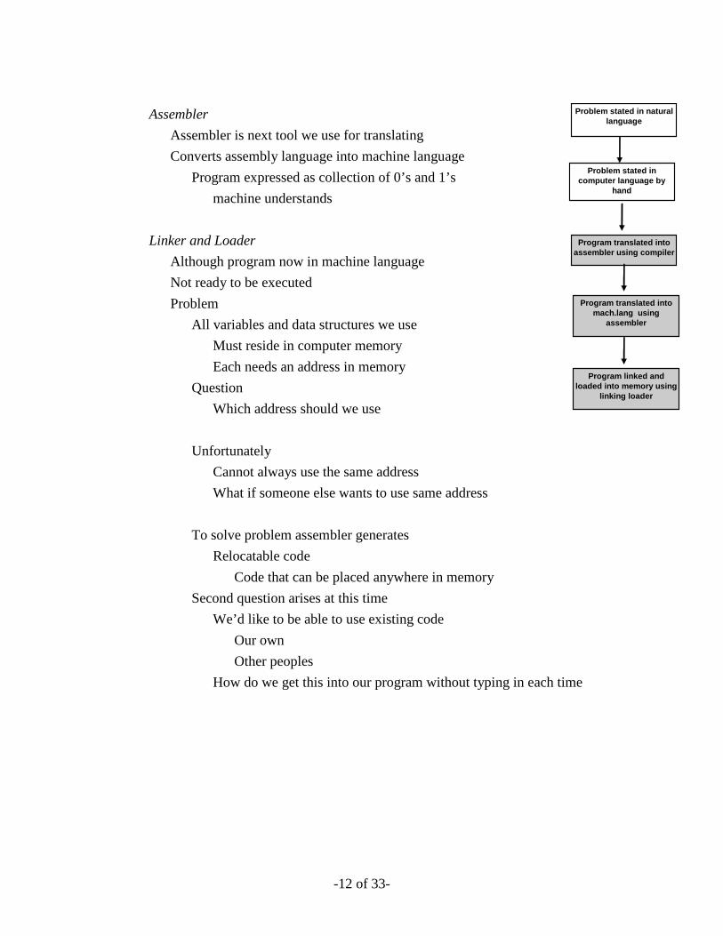
Assembler

Assembler is next tool we use for translating Converts assembly language into machine language

Program expressed as collection of 0’s and 1’s machine understands

Linker and Loader

Although program now in machine language Not ready to be executed Problem

All variables and data structures we use Must reside in computer memory Each needs an address in memory

Question Which address should we use

Unfortunately

Cannot always use the same address What if someone else wants to use same address

To solve problem assembler generates Relocatable code

Code that can be placed anywhere in memory Second question arises at this time

We’d like to be able to use existing code Our own Other peoples

How do we get this into our program without typing in each time

Problem stated in natural language

Problem stated in computer language by

hand

Program translated into assembler using compiler

Program translated into mach.lang using

assembler

Program linked and loaded into memory using

linking loader

-13 of 33-

Tool called linker loader can help with both problems Does two jobs

1. Links collection of program modules together 2. Resolves address problems

Adding that step to flow we now have

3. Into Memory Not quite there yet

Several more stages to go At this point linker and loader have gotten program into memory

PC systems this means onto the hard drive

We will see shortly Memory in embedded comprised of hierarchy of elements Some of these include

ROM - Flash RAM CACHE Registers Instruction register

Adding these we come up with We have now seen how to take problem

Expressed in natural language Turn into something that can be solved by computer

In embedded application

Solution – executable typically stored in non-volatile memory Rom / Flash

Problem stated in natural language

Problem stated in computer language by

hand

Program translated into assembler using compiler

Program translated into mach.lang using

assembler

Program linked and loaded into memory using

linking loader

Program copied from ROM into RAM

Program goes from RAM to CACHE

Program lgoes from cache to Instruction Register

-14 of 33-

Embedded Systems – An Instruction Set View Specific set of instructions for microprocessor

Called instruction set Includes instructions that

Bring data in from outside world Output signals to external world Provide means to exchange data

With memory subsystem Perform arithmetic operations

Also known as assembly language for machine For new processor design

Instructions selected and designed first These lead to or dictate architecture

Such an architecture called Instruction Set Architecture - ISA

Generally when we write embedded system program Done in high level language

C, C++ Rather than assembly language

For the machine on which we’re working On occasion we will write combination

Done when portions of programs Optimized for

Speed Size

When working with assembly language We work directly with microprocessor’s

Various registers Consequently

Must have knowledge of machine’s hardware architecture Assembly language instructions

Translated into machine code

-15 of 33-

By assembler Machine code reflects binary encoding

Machine’s instructions

Anatomy of a Machine Instruction Let’s now look at basic structure of assembly instruction At highest level machine instruction

Machine instruction contains following information Operation the instruction is to perform

Referred to as operation code Shortened to op-code

Operand information

Operands are pieces of data the Microprocessor is operating on

Typical machines support instructions Involve

One, two, or three operands Known as

One, two, or three operand (or address) instructions Each such operand has an address

Consequently also known as One, two, or three address instructions

From register’s point of view

Instructions known as Store Transfer Operate

We depict these graphically as shown Observe that we have one instruction

With no apparent address Such instructions support actions such as

NOP – no operation

OP-CODE

OP-CODE Address 1

OP-CODE Address 1 Address 2

OP-CODE Address 1 Address 2 Address 3

-16 of 33-

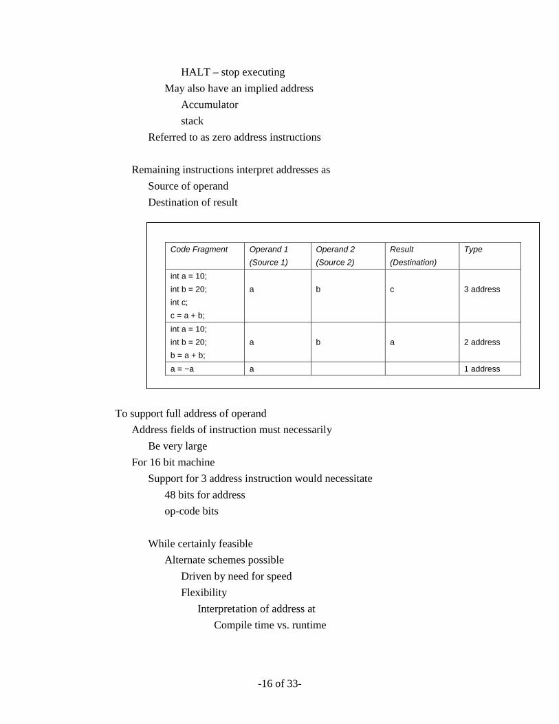
HALT – stop executing May also have an implied address

Accumulator stack

Referred to as zero address instructions Remaining instructions interpret addresses as

Source of operand Destination of result

To support full address of operand

Address fields of instruction must necessarily Be very large

For 16 bit machine Support for 3 address instruction would necessitate

48 bits for address op-code bits

While certainly feasible Alternate schemes possible

Driven by need for speed Flexibility

Interpretation of address at Compile time vs. runtime

Code Fragment Operand 1

(Source 1) Operand 2 (Source 2)

Result (Destination)

Type

int a = 10; int b = 20; a b c 3 address int c; c = a + b; int a = 10; int b = 20; a b a 2 address b = a + b; a = ~a a 1 address

-17 of 33-

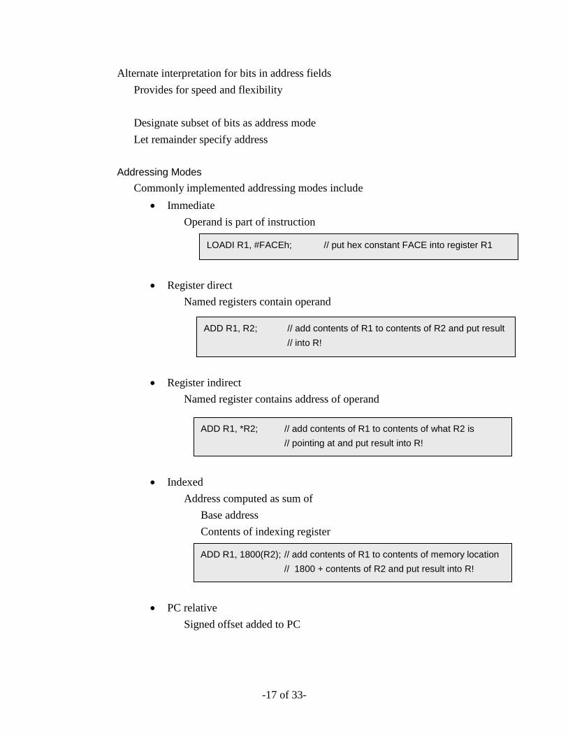
Alternate interpretation for bits in address fields Provides for speed and flexibility Designate subset of bits as address mode Let remainder specify address

Addressing Modes Commonly implemented addressing modes include

• Immediate Operand is part of instruction

• Register direct

Named registers contain operand

• Register indirect

Named register contains address of operand

• Indexed

Address computed as sum of Base address Contents of indexing register

• PC relative

Signed offset added to PC

LOADI R1, #FACEh; // put hex constant FACE into register R1

ADD R1, R2; // add contents of R1 to contents of R2 and put result // into R!

ADD R1, *R2; // add contents of R1 to contents of what R2 is // pointing at and put result into R!

ADD R1, 1800(R2); // add contents of R1 to contents of memory location // 1800 + contents of R2 and put result into R!

-18 of 33-

Becomes address of next instruction

Different vendors implement Addressing modes in different ways May have variations on fundamental scheme

Flow of Control

We can now use various addressing schemes To alter the flow of control through program

Often use information stored in flag register Holds condition codes

Values set following execution of each instruction Zero, overflow, carry…

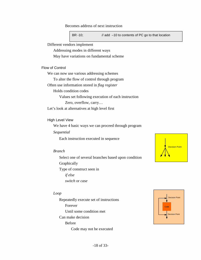
Let’s look at alternatives at high level first High Level View

We have 4 basic ways we can proceed through program

Sequential Each instruction executed in sequence

Branch Select one of several branches based upon condition Graphically Type of construct seen in

if else switch or case

Loop Repeatedly execute set of instructions

Forever Until some condition met

Can make decision Before

Code may not be executed

BR -10; // add –10 to contents of PC go to that location

Decision Point

Decision Point

Decision Point

Code

-19 of 33-

After loop Code executed at least once

Type of construct seen in do or repeat while for

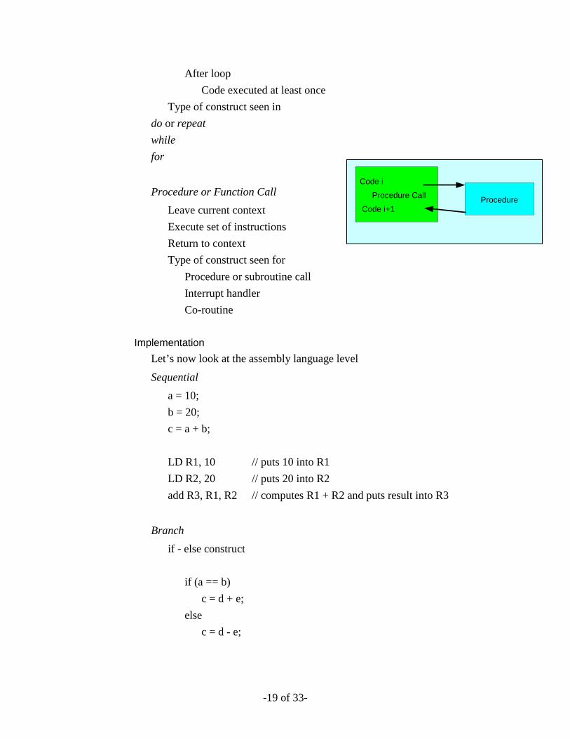
Procedure or Function Call Leave current context Execute set of instructions Return to context Type of construct seen for

Procedure or subroutine call Interrupt handler Co-routine

Implementation

Let’s now look at the assembly language level

Sequential a = 10; b = 20; c = a + b; LD R1, 10 // puts 10 into R1 LD R2, 20 // puts 20 into R2 add R3, R1, R2 // computes R1 + R2 and puts result into R3

Branch if - else construct

if (a == b) c = d + e;

else c = d - e;

Code i

Procedure Call

Code i+1Procedure

-20 of 33-

Assume a .. e in registers R1..R5

CMP R2, R1 // test if contents of R1 and R2 equal JE $1 // if equal branch to $1 // $1 is a label created by compiler SUB R3, R4, R5 // compute d - e and put results in c BR $2 // $2 is label created by compiler

$1: ADD R3, R4, R5 // compute d - e and put results in c $2: ...

Loop while (a < 10) {

i = i + 2; a++;

}

Assume a in R2 and i in R3

$1: CMP R2, 10 // test if R2 < 10 JGE $2 // if R2 greater than or equal 10 branch to $2 ADD R3, 2 // compute i + 2 put result in i ADD R2, 1 // auto increment a note an int is 4 bytes j $1 // continue looping

$2: ....

Procedure Call Most complex of flow of control constructs Not more difficult

More involved Will include

Procedures Subroutines Co-routines

-21 of 33-

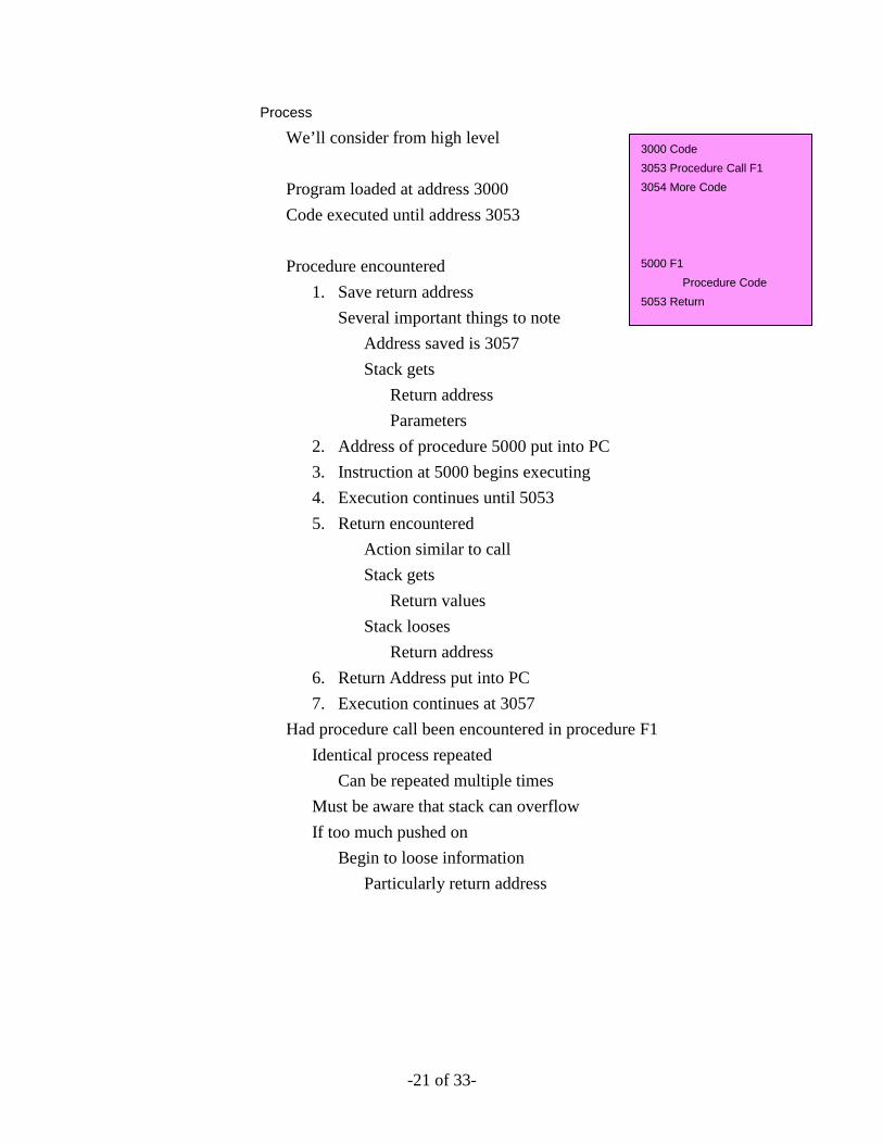
Process

We’ll consider from high level Program loaded at address 3000 Code executed until address 3053 Procedure encountered

1. Save return address Several important things to note

Address saved is 3057 Stack gets

Return address Parameters

2. Address of procedure 5000 put into PC 3. Instruction at 5000 begins executing 4. Execution continues until 5053 5. Return encountered

Action similar to call Stack gets

Return values Stack looses

Return address 6. Return Address put into PC 7. Execution continues at 3057

Had procedure call been encountered in procedure F1 Identical process repeated

Can be repeated multiple times Must be aware that stack can overflow If too much pushed on

Begin to loose information Particularly return address

3000 Code 3053 Procedure Call F1 3054 More Code 5000 F1 Procedure Code 5053 Return

-22 of 33-

Stack

Stack data structure Occupies an area in memory Has finite size and several operations Push

Puts something onto top of stack Top of stack is special value

Saved for ongoing operations

Push operation Writes something to memory Increments address of top of stack

Ready for next push

For ease of implementation Stack typically implemented from

Lower memory addresses to higher memory addresses Pop

Takes something off the top of stack Pop operation

Removes something from top of stack by Decrementing top of stack Returning previous top of stack

Peek

Looks at something on the top of stack Peek operation

Returns something from top of stack by Does not decrement top of stack

-23 of 33-

Stack Frame

Item being pushed onto or popped from stack Data structure called stack frame Special area set aside in memory for such purpose

Will not go into details at moment of Implementation Handling

Sufficient to say Contains

• Return address • From calling context

Register values Local variables Passed parameters

• From return context Values to be returned

Management

Created when procedure called Pointer

To stack frame returned Pointer placed on stack

Expanding Op-Codes

In discussion above We’ve assumed op-code field fixed

No reason for this to be the case Consider high level strategy

Similar to encoding data for transmission Make most frequently sent the simplest

Analogous to Hoffman encoding

-24 of 33-

At outset of design Designers examine necessary capabilities for system Entails identifying

What kinds of instructions to support How many of each kind

Recall our earlier discussion How many of each operand type

May need only few 1 address instructions Many 2 address versions Somewhat fewer 3 address implementations

Forcing all op-code fields to be same width

Wasteful Consider logically subdividing op-code field

Into subfields

Devote portion to encoding intended operation Let remainder distinguish amongst types Now consider how we might interpret such a field

One possibility Assume we need a large number of 2 address instructions Let MSB distinguish between

Two address (operand) instruction Not two address instruction

Second MSB or two MSBs Distinguish amongst remaining types

Now we can specify If two address instruction

Most significant m bits express op-code If not two address instruction

Most significant k bits express op-code

-25 of 33-

As designers We have perfect knowledge

What bits represent How to interpret them

Embedded Systems – A Register View

Let’s now continue moving down to the register level Know as RTL – Register Transfer Level To see how instructions are executed

Registers one of fundamental elements of microprocessor system We define 3 basic operations on data in system

All involve registers Operations

• Store data • Transfer data • Operate on data

Instructions are implemented By movement of data through registers

Using register view of system Simplifies and aides understanding

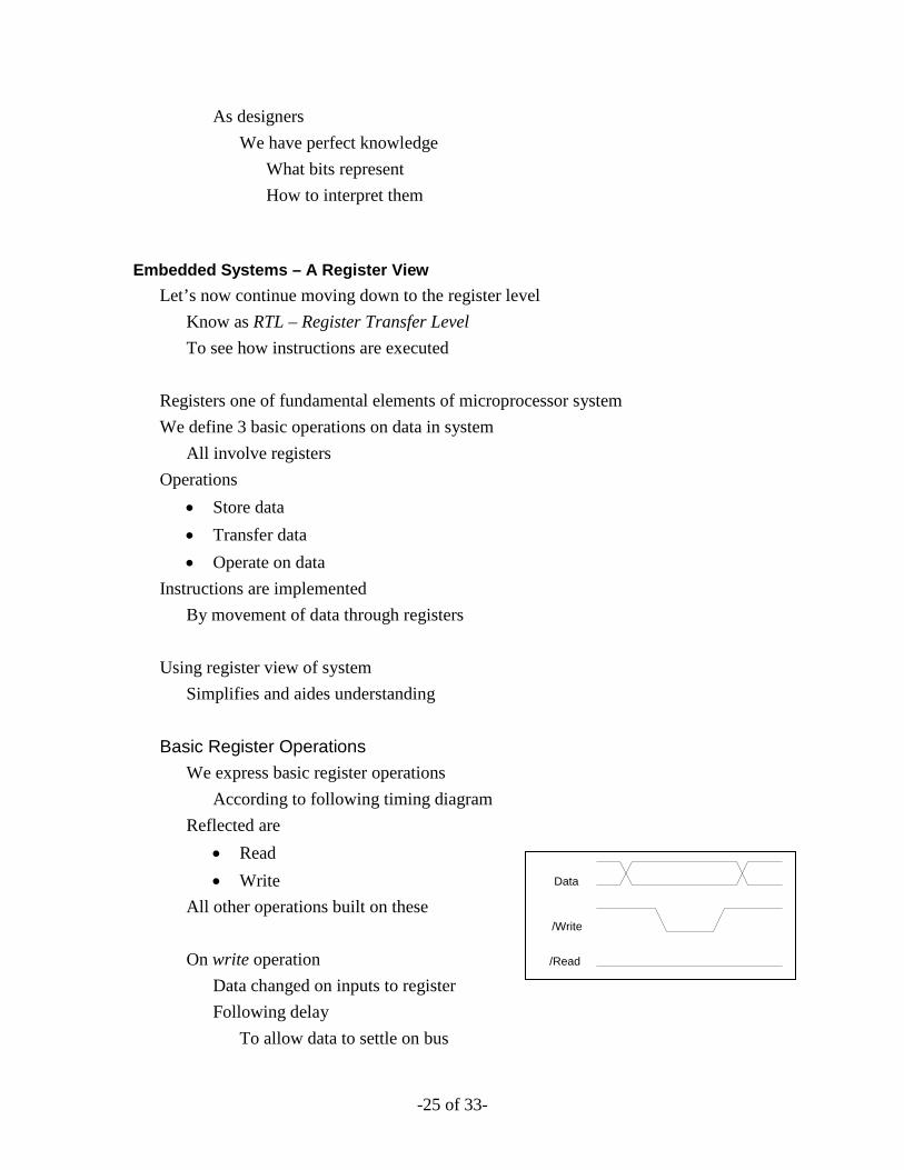
Basic Register Operations We express basic register operations

According to following timing diagram Reflected are

• Read • Write

All other operations built on these On write operation

Data changed on inputs to register Following delay

To allow data to settle on bus

Data

/Write

/Read

-26 of 33-

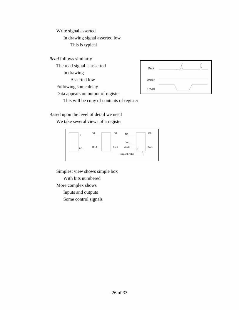
Write signal asserted In drawing signal asserted low

This is typical Read follows similarly

The read signal is asserted In drawing

Asserted low Following some delay Data appears on output of register

This will be copy of contents of register Based upon the level of detail we need

We take several views of a register

Simplest view shows simple box

With bits numbered More complex shows

Inputs and outputs Some control signals

Data

/Write

/Read

D0

Dn-1

D0

Dn-1

D0

Dn-1

D0

Dn-1

clock

Output Enable

0

n-1

-27 of 33-

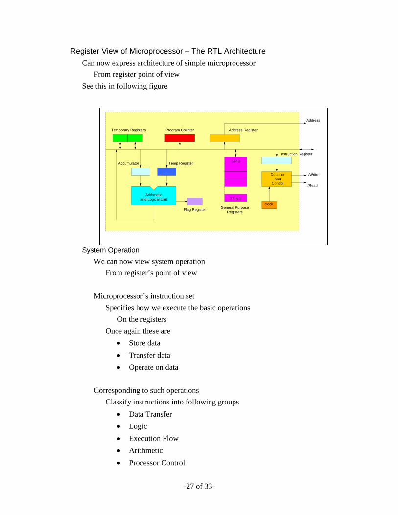
Register View of Microprocessor – The RTL Architecture Can now express architecture of simple microprocessor

From register point of view See this in following figure

System Operation We can now view system operation

From register’s point of view

Microprocessor’s instruction set Specifies how we execute the basic operations

On the registers Once again these are

• Store data • Transfer data • Operate on data

Corresponding to such operations

Classify instructions into following groups • Data Transfer • Logic • Execution Flow • Arithmetic • Processor Control

clock

GP 0

GP n-1

Temporary Registers Program Counter Address Register

Arithmeticand Logical Unit

Accumulator Temp Register

Flag Register General PurposeRegisters

Instruction Register

Decoderand

Control

/Write

/Read

Address

-28 of 33-

We express instructions Assembly level – ISA level Register transfer level – RTL level

Following table gives representative examples Each kind of instruction

One Bus Architecture Let’s explore how this may look inside the computer From name we see design has single bus

Made up of • Data • Address • Control

Type Instruction Assembler - ISA Register Transfer - RTL

Data Transfer

move register MOV R1,R2 R1 ← R2

move from memory MOV R1,memadx R1 ← (memadx)

move to memory MOV memadx, R1 (memadx) ← R1

move immediate MVI R1,#DEAD R1 ← #DEAD

Logic complement accumulator

CMA A ← !A

AND register AND R1 A ← A ∧ R1

OR register OR R1 A ← A ∨ R1

Execution Flow

unconditional jump JMP $1 PC ← $1

conditional jump J<cond> if<cond> == 1 PC ← $1

Arithmetic ADD register with carry

ADD R1 A ← A + R1 + C

Clear carry CLC C ← 0

Program Control

Don’t execute an instruction

NOP

Stop executing instructions

HALT

-29 of 33-

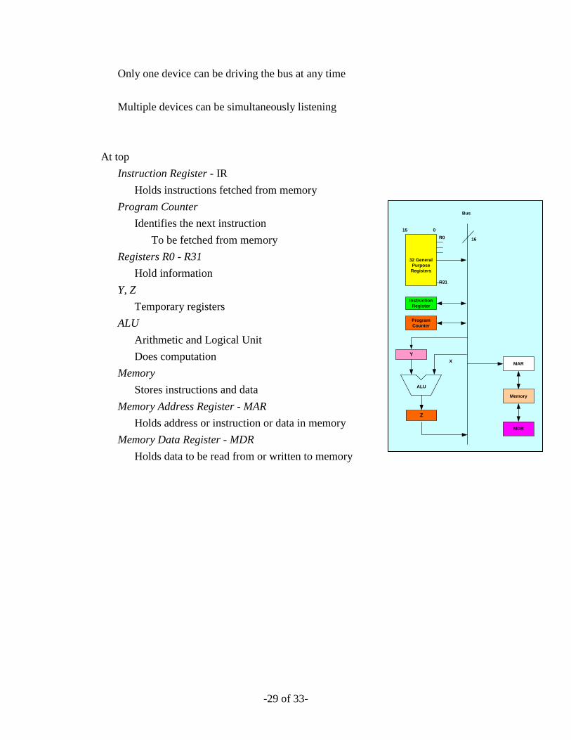
Only one device can be driving the bus at any time Multiple devices can be simultaneously listening

At top

Instruction Register - IR Holds instructions fetched from memory

Program Counter Identifies the next instruction

To be fetched from memory Registers R0 - R31

Hold information Y, Z

Temporary registers ALU

Arithmetic and Logical Unit Does computation

Memory Stores instructions and data

Memory Address Register - MAR Holds address or instruction or data in memory

Memory Data Register - MDR Holds data to be read from or written to memory

Program Counter

Instruction Register

Y

ALU

X

15 0R0

R31

32 General Purpose Registers

Bus

16

Memory

MDR

MAR

Z

-30 of 33-

Instruction Execution Cycle Instruction execution cycle comprised of 4 basic steps

Fetch Fetch instruction Next Compute address of next instruction Decode Decode current instruction Execute Execute current instruction

Can describe according to following state diagram Operation

Fetch Place address of instruction from PC onto Bus Store contents of BUS into MAR Issue a READ command Place contents of memory location into MDR Place MDR onto BUS Store contents of Bus into IR

Next Place contents of PC onto Bus Place 1 into Y register Add contents of Y and Bus in ALU Place output of ALU into Z register Place contents of Z register onto Bus Store contents of Bus into PC

Decode

Decode OP Code field Execute

Do the sequence of steps to perform the instruction

Fetch

Next

Decode

Execute

-31 of 33-

Let’s look at the sequence of operations necessary to execute a simple instruction In assembler

ST *R1, R2 This is a move indirect instruction

Use the contents of register R1 as an address in memory Read what’s at that location in memory Place the value in R2

Recall the instruction cycle

Fetch, Next, Decode, Execute

Let’s assume we’ve done the fetch part and the instruction is in the IR We now first walk through the sequence of operations

Note the control signals that are active at each step We read / write from/to a register by

Selecting it Issuing the Read / Write control signal

We assume all such actions are synchronized to the system clock

Next Place 1 on input to Y register Write to Y register Read to PC register Command ADD to ALU to Add contents of Y and Bus in ALU Place output of ALU on input to Z register Write to Z register Read from Z register Write to PC

Decode Decode the opcode ST Routed to collection of control logic called microprogram

Knows how to execute each assembler instruction

-32 of 33-

Execute

Read from R1 onto the Bus // Instruction contains adx of R1 // and info for indirect addressing

Write to MAR // Specified in microcode for ST READ to memory Wait Write to MDR Read from MDR Write to R2 // Instruction contains adx of R2

// and info for direct addressing Observe that we’ve indicated all actions happen in strict sequential order In fact number of operations can be combined to happen at same time

Provided actions don’t require same resource • Cannot

Read from two different sources at same time Both require bus

• Can Write to two different destinations Read from one and write to another

Summary We’ve looked at

High level view of computing elements Distinguished

• Microprocessors • Microcomputers • Microcontrollers

Introduced the concept of embedded systems Taken an overview of such systems Seen how time plays role in

Behaviour of such systems Notions of

Soft real time Hard real time

-33 of 33-

Explored system architecture Distinguished

Hardware Software Firmware

Seen the embedded systems development cycle Examined various views of embedded systems

Register view Firmware view

Instruction formats

Addressing modes