air table experimental set (student's...

Air Table Experiments

1

Air Table Experimental Set

(Student's Guide)

Ankara-2013


2

PACKING LIST

1. The Air Table

1.1. The Flat Plane

1.2. Spark Timer

1.3. Spark Timer Switches

1.3. Pucks

1.4. Compressor

1.5. Shooter

1.6. Carbon Paper

1.7. Foot Leveling Block

2. Connection Cables:

2.1. Power Cable

2.2. Compressor Power Cable, 220V (AC)

2.3. Footswitch Cables for the Puck and Spark Timer


3

Purpose:

The main purpose of this experiment is to study

and analyze:

I. The position and velocity of the motion

with constant velocity,

II. The acceleration of a straight-line motion

with constant acceleration,

III. Horizontal projectile (two-dimensional)

motion of an object moving on an inclined

air table,

IV. Conservation of linear momentum.

Introduction to the Air Table

The air table consists of four main components:

the flat plane, spark timer, pucks and compressor

(Figure-1).

1. The Flat Plane: With a very smooth

surface. Black carbon paper and white

recording paper are placed on it (55x55

cm).

2. Spark Timer: It produces sparks with

frequencies of 10,20,30,40 and 50Hz. In

the experiments we select the frequency

10 or 20 Hz. This gives the best results.

3. Pucks: They are rigid heavy metal disks

with very smooth surfaces. A hole is

drilled at the center through which the

pressured air flows. When the

compressor is operated by pressing the

pedal, the air with pressure flows through

the holes of the puck and forms an air

cushion between the two smooth

surfaces: the plate of air table and

smooth surface of the puck. Thus the

pucks slide on the surface almost without

any friction.

There is also an electrode at the bottom of the

puck. When the spark timer is operated by

pressing its switches, then high voltage produces

sparks which causes dark spots on the white

paper with equal time intervals.

If we place a piece of paper under the puck, we

can record its trajectory by use of a spark

apparatus, which leaves a trail of dots on the

paper. The study of these dots enables us to

measure the position as a function of time for the

moving pucks.

Figure-1: Air Table Product.


4

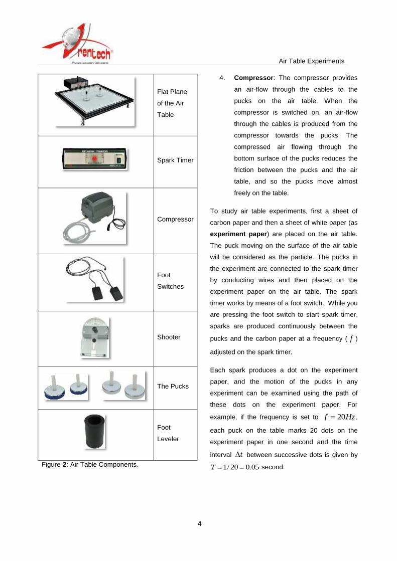
4. Compressor: The compressor provides

an air-flow through the cables to the

pucks on the air table. When the

compressor is switched on, an air-flow

through the cables is produced from the

compressor towards the pucks. The

compressed air flowing through the

bottom surface of the pucks reduces the

friction between the pucks and the air

table, and so the pucks move almost

freely on the table.

To study air table experiments, first a sheet of

carbon paper and then a sheet of white paper (as

experiment paper) are placed on the air table.

The puck moving on the surface of the air table

will be considered as the particle. The pucks in

the experiment are connected to the spark timer

by conducting wires and then placed on the

experiment paper on the air table. The spark

timer works by means of a foot switch. While you

are pressing the foot switch to start spark timer,

sparks are produced continuously between the

pucks and the carbon paper at a frequency ( f )

adjusted on the spark timer.

Each spark produces a dot on the experiment

paper, and the motion of the pucks in any

experiment can be examined using the path of

these dots on the experiment paper. For

example, if the frequency is set to Hzf 20 ,

each puck on the table marks 20 dots on the

experiment paper in one second and the time

interval t between successive dots is given by

05.020/1 T second.

Flat Plane

of the Air

Table

Spark Timer

Compressor

Foot

Switches

Shooter

The Pucks

Foot

Leveler

Figure-2: Air Table Components.


5


Experiment-1

Straight Line Motion with Constant Velocity

In this section of the experiment, you will study

and calculate the velocity of an object moving in a

straight line with constant velocity.

Theory

When a particle moves along a straight line, we

can describe its position with respect to an origin

(0), by means of a coordinate (such as x). If there

is no net force acting on a moving object, it

moves on a straight line with a constant velocity

The particle’s average velocity ( avv ) during a time

interval )( 12 ttt is equal to its displacement

)( 12 xxx divided by t :

t

x

tt

xxvav

12

12 (1)

From the Equation-(1), the average velocity is the

displacement (x) divided by the time interval (t)

during which the displacement occurs. If we plot a

graph x versus t , then we will have a straight line

with a slope. The slope of the line gives the

average velocity of the motion.

Figure-3: Position as a function of time.

For a displacement along the x-axis, the average

velocity ( avv ) of the object is equal to the slope of

a line connecting the corresponding points on the

graph of position versus time ( graphtx ). The

average velocity depends only on the total

displacement ( x ) that occurs during the motion

time )(t . The position, )(tx of an object moving

in a straight line with constant velocity is given as

a function of time as:

vtxtx 0)( (2)

If the object is at the origin with the initial position

00 x , the equation of the motion becomes at

any time:

vttx )( (3)

So, the object travels equal distance in the equal

time intervals along a straight line (Figure-3).

Name

Department

Student No

Date


6

Figure-4: The schematic representation of the experimental set-up with connection cables

electrically connected to the air table.


7

Caution!

Do not touch any metal or carbon paper and also

puck cable while spark timer is working. You

may receive an electrical shock that is not

dangerous but continues continuous exposure

may be harmful.

Experimental Procedure

1. Level the air table glass plate

horizontally by using the adjustable legs.

2. Place the black carbon paper (50x50 cm)

which is semiconducting on the glass

plate. The carbon paper should be flat

and on the air table given by the

experimental set-up (Figure-4).

3. Place white recording paper as data

sheet on the flat carbon paper.

4. Place two pucks on white paper. Keep

one of the pucks stationary on a folded

piece of data sheet at one corner of the

air table.

5. For the alignment of the air table, adjust

the legs of the air table so that the puck

will come to rest about the center of the

table.

6. Test both two switches for the

compressor and spark timer operations.

With the puck pedal, the single puck

should move easily, almost without

friction when compressor works. When

the spark timer foot switch is pressed,

black dots on white paper should be

observed (on the side that faces the

carbon paper).

7. Set the spark timer to Hzf 20 .

8. Now again, test the compressor only by

pressing the puck footswitch. Make sure

that the puck is moving freely on the air

table. By activating both the puck pedal

and spark timer pedal (foot switches) in

the same time, test also the spark timer

and observe the black dots on the

recording paper.

9. Place the puck at the edge of the table

then press both compressor and spark

timer pedals as you push the puck on the

surface of air table. It will move along the

whole diagonal distance across the air

table in a straight line with constant

velocity. Then, stop the pedals.

10. Remove the white recording paper from

air table. The dots on the data sheet will

look like those given in the Figure-(5).

11. Measure the distances of the dots

starting from first dot by using a ruler.

12. Find also the time corresponding to each

dot. The time between two dots is 1/20

seconds since the spark timer frequency

was set to Hzf 20 .

Figure-5: The dots produced by the

puck on the data sheet.


8

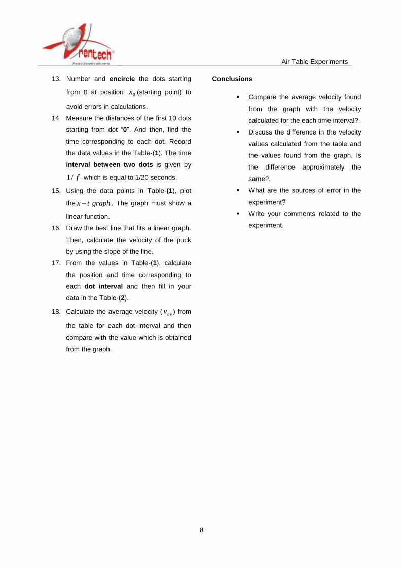
13. Number and encircle the dots starting

from 0 at position 0x (starting point) to

avoid errors in calculations.

14. Measure the distances of the first 10 dots

starting from dot “0”. And then, find the

time corresponding to each dot. Record

the data values in the Table-(1). The time

interval between two dots is given by

f/1 which is equal to 1/20 seconds.

15. Using the data points in Table-(1), plot

the graphtx . The graph must show a

linear function.

16. Draw the best line that fits a linear graph.

Then, calculate the velocity of the puck

by using the slope of the line.

17. From the values in Table-(1), calculate

the position and time corresponding to

each dot interval and then fill in your

data in the Table-(2).

18. Calculate the average velocity ( avv ) from

the table for each dot interval and then

compare with the value which is obtained

from the graph.

Conclusions

Compare the average velocity found

from the graph with the velocity

calculated for the each time interval?.

Discuss the difference in the velocity

values calculated from the table and

the values found from the graph. Is

the difference approximately the

same?.

What are the sources of error in the

experiment?

Write your comments related to the

experiment.


9

LABORATORY REPORT

Table-1: Data values for the position and time of the motion with constant velocity.

Dot Number Position )(mxx Time .)(sect )/( smvav

Slope

0 0 0

……

1

2

3

4

5

6

7

8

9

10

Table-2: Experimental data values for the average velocity of the motion with constant velocity.

Interval Number

(n) )(mxn )(1 mxn )(1 mxx nn .)(secnt )(1 stn )(1 stt nn

)/( smv

0-1 0 0 0 0 0

1-2

2-3

3-4

4-5

5-6

6-7

7-8

8-9

9-10

(Note that nx is the position of the thn data point corresponding to the related dot).


10

Experiment-2

Straight Line Motion with a Constant Acceleration

In this part of the experiment, you will examine

straight-line motion of an object (puck) with

constant acceleration on an inclined frictionless

air table. By plotting the experimental data, you

will find the acceleration of the puck sliding down

on an inclined air table.

Theory

When a particle slides straight down a frictionless

inclined plane, its acceleration is constant, and it

will move in a straight line down the plane. The

magnitude of the acceleration depends on the

angle at which the plane is inclined. If the

inclination angle is 900, the object will slide down

with an acceleration which is equal to the Earth’s

gravitational acceleration g with the magnitude

of 9.8 m/s2.

In this experiment, we will observe the motion of

a puck moving in a straight line with a velocity

changing uniformly. The back side of the air table

is raised to form an inclined plane on the air table.

The air table is inclined at an angle of with the

horizontal plane as shown in the Figure-(6).

If you put the puck at the top of the inclined air

table and let it slide down the plane, it will move

downwards on a straight line but with increasing

velocity. The rate of change of the velocity is the

acceleration of the puck. If at time 1t , the puck is

at the point 1x with a velocity of 1v , then at a

later time 2t , it will be at a point of 2x with a

velocity 2v .

The average acceleration of the puck in this time

interval 12 ttt is defined as:

12

12

tt

vv

t

vaav

(4)

Suppose that at an initial time 01 t , the puck is

at the position of 0x and has a velocity of

01 vv . At a later time tt 2 , it is in position x

and has a velocity of vv 2 . Then, the average

acceleration will be equal to:

0

0

t

vvaav

(5)

Then, the velocity of the puck will be:

atvv 0 (6)

If we consider the instantaneous acceleration

(simply the acceleration) of the motion in the x -

direction, it would be:

dt

dv

t

va t

0lim (7)

Figure-6: The straight down motion on an

inclined air table.


11

The instantaneous acceleration in a straight line

motion equals the instantaneous rate of change

of velocity with time.

The equitation for an object’s motion with

constant acceleration in one dimension )(x :

2

002

1attvxx (8)

where:

0x : The displacement at time t = 0 (initial

displacement),

0v : The speed at time t = 0 (initial speed) and,

a : The object’s acceleration.

If the motion of object starts from rest

)0,0( 00 vx at 0t , the object’s position at

any time t (instantaneous position) will be:

2

2

1atx

(9)

A graph of Equation-(9), that is, a graphtx

for motion with constant acceleration, is always a

parabola that passes through the origin in the

yx plane. However, If a graph of 2tx is

plotted, we find a straight line which has a slope

of "2

1" a and it will pass through the origin.


1. To perform this experiment, first place a

sheet of carbon paper and then a sheet

of white paper on the air table.

2. Place the foot leveler to the upper leg of

the air table to give an inclination angle

(the angle with the horizontal plane) as

09 . Use an angle finder to measure

the inclination angle.

3. Put the puck at the top of the inclined

plane and press the compressor pedal

and check if the puck is falling freely.

4. Set the spark timer frequency to

Hzf 20 .

5. Put the puck at the top of the inclined

plane to start the experiment. Press both

puck and spark timer switches

simultaneously and stop pressing when

the puck reaches the bottom part of the

inclined plane.

6. Remove the data recording paper from

air table and examine the dots produced

on it. Number and circle the dots from 0

to 10.

6.1. Take the first dot as your initial data

point ( 00 x , 00 t ) and the

positive axisx as direction of the

puck’s motion.

6.2. Measure and record the time t and

the positions x of the first 10 dots

starting from “0”. Record the data

values in the data Table-(3) with

respect to your initial point.

6.3. Calculate and record also 2t values

in the Table-(3).


12

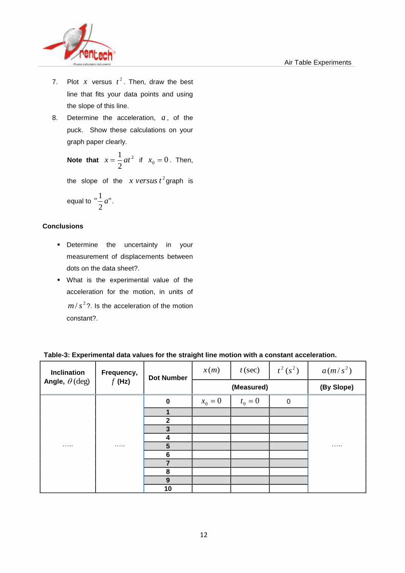
7. Plot x versus 2t . Then, draw the best

line that fits your data points and using

the slope of this line.

8. Determine the acceleration, a , of the

puck. Show these calculations on your

graph paper clearly.

Note that 2

2

1atx if 00 x . Then,

the slope of the 2tversusx graph is

equal to "2

1" a .

Conclusions

Determine the uncertainty in your

measurement of displacements between

dots on the data sheet?.

What is the experimental value of the

acceleration for the motion, in units of

2/ sm ?. Is the acceleration of the motion

constant?.

Table-3: Experimental data values for the straight line motion with a constant acceleration.

Inclination

Angle, (deg)

Frequency,

f (Hz) Dot Number

)(mx (sec)t )( 22 st )/( 2sma

(Measured) (By Slope)

….. …..

0 00 x 00 t 0

…..

1

2

3

4

5

6

7

8

9

10


13

Experiment-3

Projectile Motion

Theory

The other type of the motion in this experiment is

the horizontally projected motion. Projectile

motion is the two-dimensional motion of an

object under the influence of Earth’s gravitational

acceleration, g . The path followed by a projectile

is called its trajectory.

The position of such an object at any given time t

is given by a set of coordinates x and y which

vary with respect to time and represent the

horizontal and vertical coordinates, respectively.

One of the two components of the velocity vector

is parallel to the horizontal x-axis and the other

is parallel to the vertical, or y-axis:

jvivv yxˆˆ

(10)

The motion of the object in the horizontal x

direction is a straight line motion with constant

velocity. So, the x -component of the velocity

)( xv will be constant.

However, the acceleration only acts along the

vertical direction. The x -component of

acceleration is zero and y -component is

constant. This means that only the vertical

component of the velocity )( yv will change with

respect to time and the horizontal component of

the velocity will be constant. Therefore, we can

analyze projectile (two-dimensional) motion

as a combination of horizontal motion with

constant velocity and the vertical motion with

constant acceleration.

We can express the vector relationships for the

projectile’s acceleration by separate equations for

the horizontal and vertical components. The

components of the acceleration vector a

are:

0xa (11)

aa y (Constant) (12)

In vector form, the acceleration can be expressed

as the form:

jaa yˆ

(13)

The position of the object at a given time is given

by:

jyixr ˆˆ

(14)

For the two-dimensional ),( yx motion, we can

separate acceleration )(a , displacement )(x and

velocity v in both x and y coordinate directions

by the general equations below as:

2

002

1tatvxx xx (15)

2

002

1tatvyy yy (16)

In order to model two-dimensional projectile

motion, a metal puck will be set in motion on an

air table. When the air compressor is switched

on, the air is supplied to down the tube under the

puck so that it moves with a given initial velocity

on the frictionless plane.


14

Suppose that at time 0t , the particle is at the

point ),( 00 yx and at this time its velocity

components have the initial xv0 and yv0 . Since

the velocity of horizontal motion in the projectile

motion is constant, we find:

0xa (17)

xx vv 0 (18)

tvxx x 0 (19)

If we take the initial position )0( tat as the

origin, then:

000 yx (20)

Using this relationship in the Equation-(19), we

will find the equation of motion along the

axisx as:

tvx x

(21)

For the motion along the axisy , the velocity

)( yv at the later time, t becomes:

atvy (22)

2

2

1aty

(23)

The dots produced on the data sheet will look like

the figure as shown in the Figure-(7). Here, note

that the intervals between the dots of the x -

projections in the horizontal direction are equal.

The projectile motion has a constant horizontal

velocity and a constant vertical (downward)

acceleration due to gravity. The vertical

distance )(y caused by the change in the

velocity is given by Equation-(23). Finally, if you

analyze the projectile motion, you can make the

following important conclusions:

The horizontal component )( axisx of a

projectile’s velocity is constant. (So, the

horizontal component of acceleration, in

other words, is zero).

The projectile motion will have a constant

downward )( axisy acceleration due to

gravity as seen in the Figure-(7).

Figure-7: Schematic diagram of the horizontally

projected motion of the puck on an inclined air

table.


15


1. Place the foot leveling block at the upper

leg of the air table to give the plane an

inclination angle of 09 .

2. Adjust the frequency of the spark timer,

Hzf 20 .

3. Keep one of the pucks stationary on a

folded piece of data sheet paper and

carbon paper at the lower corner of the

plane.

4. Attach the shooter to the upper left side

of the table with 00 (zero degrees)

shooting angle to give horizontal

shooting.

5. Make test shootings to find the best

tension of the rubber to give a convenient

trajectory.

6. First activate the compressor pedal and

as you release the puck from the shooter

also start the spark timer by pressing its

pedal. Stop pressing both pedals when

pucks reach the bottom of the plane.

These dots are the data points of the

trajectory- A .

7. Now, place the puck opposite to the

shooter without tension of shooter (note

that the puck must be outside the

shooter). Then activate both compressor

pedal and spark timer pedal in the same

time and then let it slide freely down on

the inclined plane. The dots will give

trajectory- A .

8. Remove the data sheet and examine the

dots of trajectory. You must get the

trajectories illustrated in Figure-(8). If the

data points are inconvenient to analyze,

repeat the experiment and get new data.

9. Select a clear dot on the path as the

initial position of the motion as 0y

and 0t .

9.1. Circle and number the data points

(dots starting from the first dot as 0)

as 0, 1, 2, 3, 4, 5…10 as shown in

the Figure-(8).

9.2. Consider the downward trajectory as

positive axisy and horizontal

projection as positive axisx .

10. Draw perpendicular lines from dots to

axisyandx for the trajectory- B by

taking the first dot (dot 0) as the origin

)0,0( . This origin is the initial position of

the projectile motion.

11. Measure the horizontal )(mx and

vertical )(my displacements from the

initial position )0,0( and then record in

the experimental data tables.

Figure-8: The dots as data points produced by

the puck on the data sheet.


16

12. Determine the time )(t for each of these

dots. The time interval between two dots

is given by f/1 which is equal to 1/20

seconds. Then, calculate total time of

flight )( ft corresponding to the total

horizontal displacement )( Rx of a

projectile.

13. Calculate and record the horizontal

velocity )( xv by using the time of flight

)( ft and the total horizontal distance

traveled during the motion )( Rx .

Complete the data Table-(4).

14. Starting from dot “0” of the trajectory-B,

measure the distances of the y

projections (y-axis) of the first 10 data

points (dots). Determine also the times

corresponding to each of these dots.

14.1. Fill the measurements in the

trajectory-B columns in the

experimental data Table-(5).

15. Similarly, by starting from dot “0” of the

trajectory-A, measure the distances of

the y -projections of the first 10 data

points (dots).

15.1. Calculate the times

corresponding to each of the dots

for trajectory-A.

15.2. Record your data values in the

trajectory-A columns in the

Table-(5).

16. Using the equation 2

2

1aty , find the

accelerations Aa and Ba of the vertical

motions for both trajectory-A and B. In

the calculations, take displacement- y as

the total distance of the first 10 dots

starting from the dot-0 on the axisy .

17. Compare these two accelerations of both

trajectories and also compare them with

the acceleration found in the previous

experiment (Part-A).

Comments and Discussion:

Path 1 (straight line-trajectory-A):

Is the acceleration constant for the

motion along the axis?

Path 2 (curved line- trajectory-B):

Is the horizontal velocity of a projected

puck constant? Use your graph and data

sheet for your explanation.

What is the horizontal acceleration of a

projected puck?.

Does the vertical velocity of the object

increase downward in each time

interval?.

Is the vertical acceleration of projectile

(two-dimensional) motion constant?.


17

LABORATORY REPORT

Table-4: Horizontal velocity of the projectile motion.

Frequency,

)(Hzf

Dot

Number

Trajectory-B ( x -Horizontal Component Motion)

)(mx (sec)t )(mxR (sec)ft )/( smvx

(Measured) (Measured) (Calculated) (Calculated) (Calculated)

20

0 0 0

….. ….. …..

1

2

3

4

5

6

7

8

9

10

Table-5: The measurements of accelerations for the trajectory-A and trajectory-B.

Dot Number

Trajectory-A Trajectory-B Trajectory-A Trajectory-B

(Vertical Motion) (Vertical Motion) )( SlopetheBy )( SlopetheBy

)(my (sec)t )(my (sec)t )/( 2smaA )/( 2smaB

0 0 0 0 0 0 0

1

….. …..

2

3

4

5

6

7

8

9

10


18

Experiment-4

Conservation of Linear Momentum

Theory

If we consider a particle of constant mass, m , we

can write Newton’s second law for this particle as:

)( vmdt

d

dt

vdmF

(24)

Thus, Newton’s second law says that the net

force acting on a particle equals to the time rate

change of the combination, vm

(the product of

the particle’s mass and velocity). This

combination is called as the momentum or linear

momentum of the particle. Using the symbol p

for the momentum, we get the definition of the

momentum:

vmp

(25)

If we substitute the definition of momentum into

the Equation-(24), we get Newton’s second law

in terms of momentum:

dt

pdF

(26)

According to Equation-(26), the net force (vector

sum of all the forces) acting on a particle equals

to the time rate change of the particle’s

momentum. Since momentum is a vector quantity

with the same direction as the particle’s velocity,

we must express the momentum of a particle in

terms of its components.

If the particle has the velocity components of

),( yx vv , then its momentum components will be

),( yx pp . Then, the components of momentum

are given by:

xx mvp (27)

yy mvp (28)

If there are no external forces (the net external

force on a system is zero), the total momentum of

the system, P

(the vector sum of the momentum

of the individual particles that make up the

system) is constant or conserved. Each

components of the total momentum is separately

conserved. Remember that in any collision in

which external forces can be neglected,

momentum is conserved and the total momentum

before equals to the total momentum after. Only

in elastic collisions, the total kinetic energy

before equals to the total the kinetic energy after.

So, in an elastic collision between two bodies, the

initial and final relative velocities have the same

magnitude.

For a system with the two pucks, the total

momentum )( tP before the collision will be the

same as the total momentum after the collision if

the friction can be ignored.


19

By denoting initial momentums by the subscript

""i and final momentums by the "" f , the vector

equation for the principle of the conservation of

momentum is given by:

ftit PP ,,

(29)

ffii PPPP ,2,1,2,1

(30)

Let the velocities of the two pucks be denoted iv ,1

and iv ,2 before the collision as the initial values

and let the velocities after the collision be fv ,1 and

fv ,2 as the final values.

Then, the magnitude of the momentum of the

each puck before and after the collision will be:

ii mvP ,1,1 (31)

ii mvP ,2,2 (32)

ff mvP ,1,1 (33)

ff mvP ,2,2 (34)

In the any experiment, if we analyze the initial

and final velocities of a system with the two

particles (puck- A and B ), we get:

ffii vmvmvmvm ,22,11,22,11

(35)

where,

iv ,1 : The velocity of puck- A before collision,

iv ,2 : The velocity of puck- B before collision,

fv ,1 : Final velocity of puck- A after collision,

fv ,2 : Final velocity of puck- B after collision.

When the masses of the two pucks are equal

)( 21 mmm , conservation of the momentum

gives the velocity vector relationship:

ffii vvvv ,2,1,2,1

(36)

Equations-(35) and (36) explain that the

magnitude of the momentum will remain the

same. The directions and velocities of the

individual pucks may change, but vector sum

)( ,2,1 ii vv

of their momentums will remain

constant (total momentum is conserved).

Since the time interval )( t is constant between

the successive dots on the data sheet produced

by each puck, the distance between two adjacent

points on the trajectory of a puck will be

proportional to the velocity ( v ). So, in a given

experiment, the task of measuring the velocities

of the two pucks reduces to that of measuring

distances )(x of the dots.


20

The momentum is a vector quantity, so we need

to add two velocity vectors and to represent the

magnitude of the velocity vector. Note that:

The magnitude of a given vector in a

scaled vector diagram is depicted by the

length of the arrow.

The arrow is drawn a precise length

according to a chosen scale and should

have has an obvious arrowhead.

For example, we have a velocity vector with a

magnitude of scm /20 . Then, if the scale used

for constructing the diagram is chosen to be

scmcm /51 , the vector arrow of the velocity

vector is drawn with a length of cm4 , such that:

scmcmscmcm /20]1/)/5[(4 .

Therefore, graphical techniques of vector addition

involve drawing accurate scale diagrams to

denote individual vectors and their resultants. The

parallelogram method is a graphical technique of

finding the resultant of two vectors.

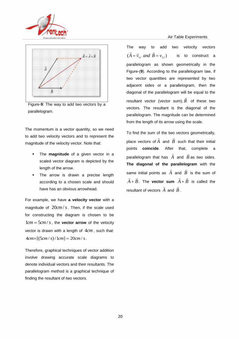
The way to add two velocity vectors

)( ,2,1 ii vBandvA

is to construct a

parallelogram as shown geometrically in the

Figure-(9). According to the parallelogram law, if

two vector quantities are represented by two

adjacent sides or a parallelogram, then the

diagonal of the parallelogram will be equal to the

resultant vector (vector sum), R

of these two

vectors. The resultant is the diagonal of the

parallelogram. The magnitude can be determined

from the length of its arrow using the scale.

To find the sum of the two vectors geometrically,

place vectors of A

and B

such that their initial

points coincide. After that, complete a

parallelogram that has A

and B

as two sides.

The diagonal of the parallelogram with the

same initial points as A

and B

is the sum of

BA

. The vector sum BA

is called the

resultant of vectors A

and B

.

Figure-9: The way to add two vectors by a

parallelogram.


21


This experiment will be carried on a level air

table. We will investigate the conservation of

momentum for two pucks moving on frictionless

horizontal air table and we will assume there is no

net external force on the system. The two pucks

will be allowed to collide and then their total

momentum before and after the collision will be

measured.

1. By adjusting the legs of the air table,

make sure it is precisely leveled.

2. Choose the spark timer frequency as

Hzf 20 .

3. Activate the compressor and spark timer

switches in the same time, and then push

the two pucks diagonally to get a collision

nearly at the center of the table. Don’t

push too slowly or too fast, you will find

the best speed after several experimental

test observations.

4. Release the two switches when they

complete their motion after the collision.

5. Remove the data sheet on the air table.

5.1. Number the dots produced by each

puck starting as 0, 1, 2, 3, 4, 5…10.

5.2. Label the two trajectories produced

by the pucks as A and B before the

collision and then A and B after

the collision. The dots of the two

pucks should look like those in the

Figure-(10).

6. Measure the total length of the two or

three intervals of the each trajectory

before and after the collision with a ruler.

7. Find the corresponding total time ( t ) of

the two or three intervals by taking the

spark timer frequency Hzf 20 .

8. Calculate the magnitude of velocity

)( vv

for each puck- A and B before

and after the collision. The magnitude of

velocity of the each puck is found by

using the total length dividing by total

time )(t . Fill your calculated data values

in the Table-(6).

Figure-10: The motion of the two pucks

before and after the collision.


22

9. Find the vector sum ii vv ,2,1

.

9.1. To find vector sum ii vv ,2,1

, extend

the trajectories A and B until they

intersect on the data sheet as seen in

the Figure-(11).

9.2. By starting from the intersection

point, draw the corresponding

velocity vectors of iv ,1

and iv ,2

along

the directions with lengths

proportional to the magnitudes of

these velocities iv ,1

and iv ,2

.

9.3. Draw a cm1 vector to represent a

velocity of scmv /10ˆ on your

data sheet or on a graph paper such

that scale: 1cm=10cm/s.

9.4. Constructing the parallelogram as

shown in the Figure-(11), add the two

velocity vectors by using

parallelogram method to find the

vector sum (resultant vector)

ii vv ,2,1

and its magnitude as

ii vv ,2,1

. Record the results in the

Table-(6).

9.5. The length of the each vector

represents the magnitude and it

points in the direction of the velocity.

10. Repeat the same procedure to find the

vector sum of ff vv ,2,1

and the

corresponding magnitude.

LABORATORY REPORT

Comments and Discussion:

1. Is the linear momentum is conserved in the collision

if no external force acts on the system?.

2. Discuss the conservation of the linear momentum

by using the data values.

Figure-11: Vector sum given

geometrically by constructing a

parallelogram.

Table-6: Conservation of the linear momentum.

)/(,1 smv i

)/(,2 smv i

ii vv ,2,1

ff vv ,2,1

air table experimental set (student's...

Documents