A COMBINED ADAPTIVE TABU SEARCH AND SET

PARTITIONING APPROACH FOR THE CREW SCHEDULING

PROBLEM WITH AN AIR TANKER CREW APPLICATION

DISSERTATION

Todd E. Combs, Captain, USAF

AFIT/DS/ENS/02-04

DEPARTMENT OF THE AIR FORCE AIR UNIVERSITY

AIR FORCE INSTITUTE OF TECHNOLOGY

Wright-Patterson Air Force Base, Ohio

APPROVED FOR PUBLIC RELEASE; DISTRIBUTION UNLIMITED.

Report Documentation Page

Report Date 15 Aug 02

Report Type Final

Dates Covered (from... to) Apr 01 - Aug 02

Title and Subtitle A Combined Adaptive Tabu Search and Set PartitioningApproach for the Crew Scheduling Problem with an AirTanker Crew Application

Contract Number

Grant Number

Program Element Number

Author(s) Captain Todd E. Combs, USAF

Project Number

Task Number

Work Unit Number

Performing Organization Name(s) and Address(es) Air Force Institute of Technology Graduate School ofEngineering and Management (AFIT/EN) 2950 P StreetWPAFB OH 45433-7765

Performing Organization Report Number AFIT/DS/ENS/02-04

Sponsoring/Monitoring Agency Name(s) and Address(es) Maj Juan Vasquez AFOSR/NM 801 N. Randolph St., Rm732 Arlington, VA 22203-1977

Sponsor/Monitor’s Acronym(s)

Sponsor/Monitor’s Report Number(s)

Distribution/Availability Statement Approved for public release, distribution unlimited

Supplementary Notes The original document contains color images.

Abstract This research develops the first metaheuristic approach to the complete air crew scheduling problem. Itdevelops the first dynamic, integrated, set-partitioning based vocabulary scheme for metaheuristic search.Since no benchmark flight schedules exist for the tanker crew scheduling problem, this research defines anddevelops a Java (TM) based flight schedule generator. The robustness of the tabu search algorithms is judgedby testing them using designed experiments. An integer program is developed to calculate lower bounds forthe tanker crew scheduling problem objectives and to measure the overall quality of solutions produced bythe developed algorithms.

Subject Terms Metaheuristics, Tabu Search, Group Theory, Crew Scheduling, Crew Scheduling Problems, Flight Schedule Generation

Report Classification unclassified

Classification of this page unclassified

Classification of Abstract unclassified

Limitation of Abstract UU

Number of Pages 174

The views expressed in this dissertation are those of the author and do not reflect the official policy or position of the United States Air Force, Department of Defense, or the U.S. Government.

AFIT/DS/ENS/02-04

A COMBINED ADAPTIVE TABU SEARCH AND SET PARTITIONING

APPROACH FOR THE CREW SCHEDULING PROBLEM WITH AN AIR

TANKER CREW APPLICATION

DISSERTATION

Presented to the Faculty

Graduate School of Engineering and Management

Air Force Institute of Technology

Air University

Air Education and Training Command

in Partial Fulfillment of the Requirements for the

Degree of Doctor of Philosophy

Todd E. Combs, B.S., M.S.

Captain, USAF

August 2002

APPROVED FOR PUBLIC RELEASE; DISTRIBUTION UNLIMITED.

AFIT/DS/ENS/02-04

A COMBINED ADAPTIVE TABU SEARCH AND SET PARTITIONING

APPROACH FOR THE CREW SCHEDULING PROBLEM WITH AN AIR

TANKER CREW APPLICATION

Todd E. Combs, B.S., M.S. Captain, US Air Force

Approved: Date ____________________________________ James T. Moore (Chairman) ____________________________________ J. Wesley Barnes (Member) ____________________________________ Lt Col Raymond R. Hill (Member) ____________________________________ Mark E. Oxley (Member) ____________________________________ Won B. Roh (Dean’s Representative)

Accepted: ______________________________ Robert A. Calico, Jr., Dean Date Graduate School of Engineering and Management

iv

Acknowledgments

I would like to express my appreciation to my faculty advisor, Dr. James Moore. His

guidance and unwavering support paved the path to success for this research effort. I

would like to thank my committee members Dr. Barnes, Dr. Oxley, and Lt Col Hill for

the time and effort spent successfully guiding my research.

Special appreciation goes to Capt Vic Wiley and Lt Rob Harder. Capt Wiley and Lt

Harder provided the group theory and tabu search JavaTM frameworks on which this

research’s code was built. They were extremely responsive in providing underlying

improvements needed for this research.

Finally, I would like to express my appreciation for the love and patience provided by

my wife, step-children, and parents throughout my research effort. This support allowed

me to overcome the obstacles that arose throughout this long venture.

Todd E. Combs

v

Table of Contents

Page Acknowledgments..........................................................................................................iv

List of Figures ..............................................................................................................viii

List of Tables .................................................................................................................ix

List of Equations .............................................................................................................x

I. Introduction..............................................................................................................1

1.1 General Discussion ............................................................................................1 1.2 Motivation .........................................................................................................1 1.3 Problem Statement .............................................................................................3 1.4 Organization of Dissertation ..............................................................................4

II Introduction to Tabu Search and Group Theory .......................................................5

2.1 Tabu Search.......................................................................................................5 2.1.1 The Basic Tabu Search................................................................................6 2.1.2 Advanced Concepts...................................................................................10

2.2 Group Theory ..................................................................................................17 2.2.1 The Basics.................................................................................................17 2.2.2 Template-based Moves..............................................................................20 2.2.3 Conjugation-based Moves. ........................................................................21

III Literature Review ..............................................................................................23

3.1 U.S. Air Force Concerns ..................................................................................23 3.2 Crew Scheduling..............................................................................................25

3.2.1 The Airline Crew Scheduling Problem. .....................................................25 3.2.2 Solving the Airline CSP. ...........................................................................28 3.2.3 Motivation for this Research. ....................................................................30 3.2.4 Solving Other CSPs...................................................................................32

3.3 Designed Experiments .....................................................................................33 IV An Adaptive Tabu Search (ATS) Approach..........................................................37

4.1 Tanker Crew Scheduling Problem....................................................................37 4.2 Components of the Adaptive Tabu Search........................................................40

4.2.1 Solution Structure. ....................................................................................40

vi

4.2.2 Initial Solution Construction......................................................................46 4.2.3 Restricted Neighborhood Construction. .....................................................49 4.2.4 Solution and Move Evaluation................................................................52 4.2.5 Tabu List...................................................................................................64

4.3 Vocabulary Building With Set Partitioning ......................................................65 4.4 Completing the ATS Framework .....................................................................68

4.4.1 One Iteration of the ATS. ..........................................................................68 4.4.2 The ATS with Intensification. ...................................................................69

V A JavaTM-based Flight Schedule Generator ............................................................73

5.1 Motivation .......................................................................................................73 5.2 The Flight Schedule Generator Components ....................................................74

5.2.1 Java Classes. .............................................................................................74 5.2.2 Java Interfaces...........................................................................................75

5.3 The Flight Schedule Generator Algorithm........................................................78 VI Analysis of the ATS and Experimental Results........................................................81

6.1 Objectives........................................................................................................81 6.2 Experimental Design........................................................................................82

6.2.1 Design Factors. .........................................................................................82 6.2.2 Responses Studied.....................................................................................85 6.2.3 The Fractional Factorial Design. ................................................................88

6.3 Determining Lower Bounds for the TCSP........................................................89 6.4 Experimental Results .....................................................................................92

6.4.1 Examination of the Factor Effects. ............................................................92 6.4.2 Comparing the ATS Solutions to Lower Bounds. ......................................98 6.4.3 Comparing ATS Solutions to Known Optimal Solutions. ........................100 6.4.4 Solving a Very Large TCSP. ...................................................................101

VII Concluding Remarks........................................................................................105

7.1 Major Contributions.....................................................................................105 7.1.1 Operations Research Contributions..........................................................105 7.1.2 USAF Contributions................................................................................106

7.2 Avenues for Future Research .........................................................................107 7.3 Conclusions ...................................................................................................109

APPENDIX A: JavaTM Components of the Flight Schedule Generator .......................110

Java Classes.........................................................................................................110 Java Interfaces .....................................................................................................112

vii

APPENDIX B: Using the Flight Schedule Generator..................................................114

APPENDIX C: Resolution IV Experimental Design...................................................119

APPENDIX D: Raw Data on Experimental Design ....................................................126

APPENDIX E: Raw Data on Crew Bounds ................................................................131

APPENDIX F: Example TCSP Bound Solution..........................................................135

APPENDIX G: ANOVA Calculations for the Designed Experiment ..........................136

APPENDIX H: Optimality Results on Smaller TCSPs................................................ 155

Bibliography ...............................................................................................................157

viii

List of Figures

Figure Page 1. One Iteration of OpenTS (Harder, 2002).................................................................10 2. A Balanced Intensification & Diversification Approach..........................................13 3. Strategic Oscillation ...............................................................................................15 4. Mapping a Symmetric Group Element to the SPP ...................................................27 5. Initial Solution Heuristic.........................................................................................48 6. Evaluation of a Single Crew ...................................................................................58 7. Evaluation of 30/90 Day Flying History for First Flight ..........................................61 8. Evaluation of 30/90 Day Flying History for Other Flights.......................................63 9. Typical Local Search ..............................................................................................65 10. ATS Local Search...................................................................................................66 11. One Iteration of OpenTS (Harder, 2002).................................................................69 12. Generating the Flight Schedules..............................................................................78 13. Generating Aircraft Rotations .................................................................................79 14. Finding the Smallest Feasible Number of Crews in a Large TCSP. .......................103 15. Finding the Smallest Total Wait Time in a Large TCSP........................................103

ix

List of Tables

Table Page

1. Crew Constraints for the Tanker CSP .......................................................................38 2. Comparison of generalized hs and the existing group theory hash function................44 3. Experimental Design Factors ....................................................................................84 4. Factor Effects for the TCSP objectives .....................................................................95 5. Factor Effects for Number of Iterations, Total Solution Time, Number of Conjucacy

Classes Visited, Ave Neighborhood Size, and Ave Tabu Tenure............................97 6. Ave and Standard Deviation for % Distance with Respect to the Lower Bounds.......99 7. Summary of Four Sub-optimal ATS Solutions in the Experimental Design.............101 8. Characteristics of a Large Deployment Operation...................................................102 9. Example Flight Schedule ........................................................................................118

x

List of Equations

Equation Page 1. Set Partitioning Problem (SPP) Formulation ...........................................................27 2. Hashing Function for a Crew Rotation....................................................................42 3. General Hashing Function for Disjoint Cycles ........................................................43 4. Solution Hashing Function for the TCSP ................................................................44 5. Conjugacy Class Hash Function..............................................................................45 6. Solution Evaluation ................................................................................................52 7. Move evaluation .....................................................................................................53 8. Penalty parameter adjustment .................................................................................54 9. Linear Penalties for TCSP Constraints ....................................................................56 10. Integer Program Used to Calculate TCSP Lower Bounds........................................91 11. Hypothesis Test for Factor Effects ..........................................................................92 12. Calculating % Distance from the Lower Bound ......................................................98

xi

AFIT/DS/ENS/02-04

Abstract

Aerial refueling is a crucial component of modern day military operations. A vital

part of this refueling process is the individual tanker crews. Constrained by the number

of tanker crews available, the United States Air Force must find ways to efficiently

schedule them.

This research develops two effective tabu search approaches to Air Mobility

Command’s tanker crew scheduling problem. The first is an adaptive tabu search with

intensification. The second is a hybrid adaptive tabu search/set partitioning scheme that

combines the metaheuristic tabu search with a classical optimization approach. The

research shows that group theory can be used to effectively direct the search process of

each algorithm.

Since no benchmark flight schedules exist for the tanker crew scheduling problem,

this research developed a JavaTM based flight schedule generator. The robustness of the

developed tabu search algorithms is judged by testing them using designed experiments.

An integer program (IP) is developed to calculate lower bounds for the tanker crew

scheduling problem objectives and to measure the overall quality of solutions produced

by the developed algorithms. The results show that either algorithm significantly

improves the solutions found by the currently used heuristic methodology.

1

A COMBINED ADAPTIVE TABU SEARCH AND SET PARTITIONING

APPROACH FOR THE CREW SCHEDULING PROBLEM WITH AN AIR

TANKER CREW APPLICATION

I. Introduction

1.1 General Discussion

This research significantly contributes to the efficient scheduling of Air Mobility

Command’s (AMC) tanker crews. The general airline scheduling problem has been

studied for over 30 years, with markedly increased interest in the last decade. Previous

research has developed extensive optimization and heuristic algorithms for the airline

crew scheduling problem, but it has focused little effort on the use of metaheuristics such

as tabu search. In addition, the United States Air Force (USAF) has focused its analytic

efforts on the scheduling of aircraft for aerial refueling and paid less attention to the crew

assignment component of the problem. This research uses the tabu search metaheuristic

to solve the USAF tanker crew scheduling problem (TCSP).

1.2 Motivation

One of the most important aspects of running an operational Air Force flying unit or

major airline is scheduling flight crews. Once the Air Tasking Order (ATO) or airline

schedule is published to specify the flights to be flown daily, crews must be intelligently

assigned to each flight. For today’s airlines, crew costs are the second highest component

2

of direct operating costs, with the fuel cost being the highest (Gershkoff, 1989:30). Crew

costs such as temporary duty (TDY) per diem are also a significant portion of the direct

operating costs of any flying unit within the U.S. Air Force, but the mission of the Air

Force contains many more important concerns. Since many flying units operate with an

insufficient number of crews, improper crew scheduling will further limit combat

operations. A recent Air Force Times article addresses this issue (Simon, 2000:10).

When lives and national interests are on the line, any increase in the probability of

mission failure is unacceptable.

In addition to cost, many other factors must be considered in tanker crew scheduling.

The USAF dictates the handling of its crews through various regulations. For example, a

crew’s flight duty period starts when an aircrew reports for a mission, briefing, or other

official duty and ends with an outbriefing following engine shut down at the completion

of a mission, mission leg, or a series of missions (AFI11-202V3, 1998:43). Air Force

Instruction 11-202 Volume 3 (AFI 11-202V3) states that the maximum flight duty period

for a tanker aircrew is 16 hours (1998:44). Many other such constraints apply to the

TCSP, and they are defined in Section 4.1. For commercial airlines, the Federal Aviation

Administration (FAA) has also established complex rules to ensure that crewmembers

fulfill their duties at an appropriate performance level.

These regulations, combined with the nature of the underlying combinatorial problem,

make the crew scheduling problem (CSP) very difficult to solve. The airlines are

constantly searching for new ways to obtain “good” crew schedules, i.e., schedules that

cover all the flights on the schedule, meet the FAA rules, meet union requirements, and

are of relatively low cost. Because civilian airline crew costs often exceed $1.3 billion

3

every year, even very small incremental savings can save the airlines a significant amount

of money each year (Hoffman and Padberg, 1993:658). The success of tabu search on

similar combinatorial problems motivates its use in this research (Barnes, et al., 1995;

Dowsland, 1998; Lourenco, et al., 1998; Shen and Kwan, 2000).

1.3 Problem Statement

A major problem facing AMC is how to efficiently schedule its tanker crews. They

have a severe shortage of tanker crews with no apparent relief projected in terms of either

more crews or reduced mission requirements. Today, AMC analysts use a simulation

program, “Crew Dog,” to determine the number of crews needed to fly a given aerial

refueling schedule (Ryer, 2000). Crew Dog embodies a simple greedy heuristic. Greedy

heuristics tend to converge to local optimal solutions, thus ignoring large portions of the

solution space. This is true of the heuristic described in Section 4.2.2, which provides a

starting solution for the tabu search approach developed in this work. Although the

greedy heuristic provides very good initial solutions, the results from Chapter VI show

that the solutions can clearly be improved.

The thrust of this research is to develop an efficient tabu search approach to AMC’s

TCSP. Tabu search allows the search to overcome the trap of local optimality and

provide more efficient crew schedules. For the two adaptive tabu search algorithms

developed, group theory provides the mechanisms to efficiently direct the metaheuristic

search process.

The robustness of the developed tabu search algorithms is judged by extensively

testing them using designed experiments and benchmark test problems. Since no

4

benchmark problem sets for the TCSP exist, construction of these experiments required

the development of a JavaTM based flight schedule generator. Finally, an integer program

(IP) to calculate lower bounds for the TCSP objectives is developed in order to measure

the overall quality of the metaheuristics.

1.4 Organization of Dissertation

The remainder of this dissertation is organized as follows. Chapter II provides an

introduction to tabu search and group theory, laying the foundation for Chapters III and

IV. Chapter III provides a review of both the USAF’s concern with crew scheduling and

the airline CSP, to include previously developed solution methodologies.

Chapter IV discusses the adaptive tabu search methodology developed to solve the

TCSP, including a hybrid methodology that uses set partitioning optimization as a

vocabulary building mechanism within the metaheuristic. Chapter V details the general

flight schedule generator developed during this research. Chapter VI provides a

designed, statistical analysis of the tabu search approaches--to include the development of

new IP-based lower bounds. Finally, Chapter VII concludes by discussing the

contributions of the research and avenues for future research.

5

II Introduction to Tabu Search and Group Theory

This chapter explains the basics of tabu search and group theory. It provides the

minimum background necessary to understand the adaptive tabu search methodology

developed in Chapter IV.

2.1 Tabu Search

Tabu search is a metaheuristic, a master strategy that forces a local heuristic search

procedure to explore the solution space beyond local optimal (Glover and Laguna,

1997:2). The fundamental philosophies of tabu search are the following:

1) Adaptive memory should be used to create a robust search methodology, unlike simulated annealing and genetic algorithms that use randomness to guide the search process.

2) The solution space should be explored intelligently, i.e., the search must respond

appropriately to what is occurring or has occurred during the search process. Section 2.1.1 describes the basic components present in any tabu search metaheuristic.

This basic tabu search mechanism is often so effective that it suffices for the problem

under investigation. Unfortunately, the basic tabu search approach fails for some

problems and the implementation of more advanced, readily available concepts is

required. Section 2.1.2 discusses the advanced tabu search concepts exploited by this

research.

6

2.1.1 The Basic Tabu Search.

Solution Structure.

The foundation of any optimization routine is the problem’s solution structure. This

structure mathematically describes the various decision variables inherent in the

optimization model and precisely defines the elements of the solution space. Section

2.2.1 describes the solution structure the symmetric group on n letters provides for this

research. Once a solution structure is chosen, the basic tabu search begins by creating an

initial solution. Section 4.2.2 describes the constructive heuristic used to create initial

solutions in this research.

The Neighborhood of Solution x.

Once the initial solution, x, is created, the metaheuristic needs a way to travel to other

solutions within the solution space. This is done by creating and examining a

neighborhood of the initial solution, x, and all subsequent solutions.

Reeves (1995:5) states, “A neighborhood N(x,σ) of a solution x is a set of solutions

that can be reached from x by a simple operation σ.” The operation σ is generally called

a “move” in tabu search applications. Implicit in the definition of N(x,σ) is M, the set of

all moves of type σ that map x to N(x,σ).

A simple example clarifies this neighborhood definition. Suppose for a 3-crew/3-

flight problem the initial solution, x, has crew 1 assigned flight 1, crew 2 assigned flight

2, and crew 3 assigned flight 3. A swap move could be used to search beyond this

incumbent solution. Define the swap move, σ, as exchanging flight i with flight j. M is

7

therefore all exchanges of flight i with flight j, for i = 1, 2 and i < j ≤ 3. Therefore,

N(x,σ) is as follows:

1) Reassign flight 2 to crew 1 and flight 1 to crew 2. Crew 3 assigned flight 3.

2) Reassign flight 3 to crew 1 and flight 1 to crew 3. Crew 2 assigned flight 2.

3) Reassign flight 3 to crew 2 and flight 2 to crew 3. Crew 1 assigned flight 1.

Choosing the Next Incumbent Solution from N(x,σ).

Once N(x,σ) has been constructed, solutions in N(x,σ) must be evaluated and one

member chosen as the next incumbent solution. The function used to evaluate solutions

within N(x,σ) generally considers the particular problem’s objectives and constraints, as

shown in Section 4.2.4. Given this method to evaluate solutions, different rules may be

used to choose the next incumbent solution from N(x,σ). For example, one tabu search

implementation may choose the first improving solution in the neighborhood while

another selects the “best” neighbor solution. The tabu search routines developed in this

research strategically exploit both of these rules.

Tabu List.

In choosing the new incumbent solution from N(x,σ), the tabu list must also be

considered. A tabu list provides the short-term memory needed to escape from a local

optimum and progress into other regions of the solution space.

Glover and Laguna (1997:31) state, “The most commonly used short-term memory

keeps track of solution attributes that have changed during the recent past.” Suppose the

first neighborhood move from the swap neighborhood previously described satisfies the

“best” criteria and is selected as the new incumbent solution. One attribute of the

8

solution is the assignment changes of crews 1 and 2. A tabu list based on this attribute

may make swaps involving crews 1 and 2 tabu for a period of time, called the tabu

tenure. Another attribute of the solution is the reassignment of flights 1 and 2. One tabu

list using this attribute may make any swaps involving flights 1 and 2 tabu for a period of

time. This is a restrictive implementation when compared to another tabu list

implementation that may only make the specific swapping of flights 1 and 2 tabu for a

period of time. The tabu list to implement is generally problem specific and an area of

research when developing a complete tabu search methodology.

Aspiration criteria provide a flexible tool to overcome the restrictive implementations

described above, and may be important to avoid not visiting good solutions. The analyst

defines the aspiration criteria conditions that must be satisfied before the tabu search

accepts a currently forbidden move. A commonly used aspiration is to allow a forbidden

move if the resulting solution quality is superior to the best found so far. Glover and

Laguna note that aspiration criteria are very important in allowing tabu search to achieve

its expected superior performance (1997:50).

Many different ways exist to represent recent solutions or moves on a tabu list and

how you define the list can significantly affect the search. A solution tabu list may be

used as an alternative to the attribute-based lists discussed above. In this case, an entire

solution is placed on the tabu list. Since storing and comparing whole solutions can take

an enormous amount of memory and time, hash values are generally used as solution

surrogates (Glover and Laguna, 1997:246-248). Chapter IV describes the solution tabu

list used within the adaptive tabu search (ATS) developed in this dissertation.

9

An Iteration of the Basic Tabu Search.

This section concludes by demonstrating an iteration of the basic tabu search, as

implemented in OpenTS, the JavaTM-based software used in this research. Figure 1

below displays an iteration of the OpenTS tabu search framework (Harder: 2002).

OpenTS starts from an initial solution defined by the user. Instead of explicitly

building the solutions defined by N(x,σ), OpenTS builds the neighborhood of moves, M.

This neighborhood of moves has a one-to-one correspondence to N(x,σ), and is generally

quicker and more memory-efficient to build.

Once the moves are created, OpenTS forwards M to the objective function evaluator.

The objective function evaluator takes each move of M and examines N(x,σ), one

element at a time, using user-defined evaluation methods. Clearly, if the next incumbent

solution is chosen as the first improving solution in N(x,σ), it is unlikely the entire

neighborhood will be evaluated and the time to evaluate N(x,σ) should decrease. Further

time efficiencies occur when elements of N(x,σ) can be evaluated incrementally, i.e.,

without completely building the neighbor solutions. Section 4.2.4 describes the

incremental evaluations used in this research.

Finally, the move chosen from N(x,σ) is used to operate on the current solution, create

the new incumbent solution, and complete an iteration of the basic tabu search.

10

Figure 1: One Iteration of OpenTS (Harder, 2002)

2.1.2 Advanced Concepts.

The basic approach described above does not always produce the best solutions. The

simple search often fails because of the combinatorial explosion in the number of

variables and constraints present in many of the problems approached by tabu search.

Such an explosion overwhelms simpler methods and does not allow the effective search

of the problem’s solution space.

For example, it would be impractical to examine the entire solution space of a scenario

with 50 flights to schedule. The solution space consists of 50! = 3.04*1064 solutions and

a computer evaluating 1 trillion solutions per second would take 1044 years to examine all

of them. Therefore, during the tabu search process, only the applicable portion of the

entire solution space need be examined explicitly.

This does not imply defeat in the face of the basic tabu search’s failure. It simply

means other strategies must be invoked. Glover and Laguna (1997) emphasized the need

11

to understand advanced strategies early in their book. They stated that, “Incorporating

only a couple of TS-related concepts into a search procedure may result in an inferior

method and a frustrating experience…Our goal, however, is to present most of the

strategic issues as early as possible in order to encourage future TS researchers and

practitioners to incorporate these concepts into their application” (Glover and Laguna,

1997:9). This section of the paper describes some of the advanced tabu search concepts

that have proved very useful in combinatorial applications.

Intensification and Diversification.

Glover and Laguna define intensification as, “Strategies based on modifying choice

rules to encourage move combinations and solution features historically found good.

They may also initiate a return to attractive regions to search them more thoroughly”

(Glover and Laguna, 1997:96).

Intensification may be implemented by modifying appropriate choice rules found

within the tabu search. For example, while conducting recency-based moves, the search

may identify move combinations or solution attributes that produce good solutions. Once

identified, the search could encourage the use of these moves or attributes to build

ensuing neighborhoods.

Another strategy for intensification is an ability to return to promising regions found

in the previous portion of the search in an attempt to find better solutions. Glover and

Laguna state that, “Since elite solutions must be recorded in order to examine their

immediate neighborhoods, explicit memory is closely related to the implementation of

intensification strategies” (Glover and Laguna, 1997:8). In other words, if you expect to

return to promising regions, you must explicitly record the solutions you may want to

12

revisit. In addition, this explicit bookkeeping must be done in a manner that does not

hinder the computational performance of the search process.

As opposed to intensification’s concentration on certain moves or promising regions,

diversification encourages the search process to examine unvisited regions of the solution

space to investigate solutions that differ significantly from those found previously.

The philosophy of diversification within tabu search is analogous to the diversification

recommended for personal investments. Financial counselors routinely tell investors to

diversify their financial portfolio by placing their money in multiple market sectors or

financial instruments. Diversification protects the investor by ensuring one poorly

performing sector does not destroy their financial interests.

Diversification within tabu search works much the same way, but the investment made

by a tabu search algorithm is the computational effort needed to solve the problem.

When a tabu search is diversified, it visits many sectors of the solution space. These

sectors, defined in Section 2.2.1 as conjugacy classes, contain many individual solutions.

While the investor lowers his financial risk by diversifying into multiple market sectors,

the tabu search lowers its risk of not identifying very good individual solutions by

visiting many of the solution space sectors.

One way to ensure diversification within the tabu search is to use long-term memory

structures that track solutions or solution attributes that have occurred earlier in the

search. Frequency data is a popular way to represent such long-term memory. For

instance, throughout the search process the tabu search may record how many times

certain sectors are visited. It may then force the search trajectory to move to sectors

previously unvisited.

13

This research uses a balanced approach to intensification and diversification. It uses

two tabu list schemes, described in Section 4.2.5, and an adaptive solution and move

evaluator, described in Section 4.2.4, to promote diversification. By using these two

components, the search avoids using long-term frequency information to explicitly force

the trajectory to particular portions of the solution space. It implements an intensification

scheme, described in Section 4.4.2, that returns to elite solutions to further search their

neighborhoods for improvements. Diversification is not ignored while completing this

intensification. The tabu search continues to allow movement to any solution space

sector. Figure 2 below displays a typical result of the intensification and diversification

approach used in this research. The number of sectors visited grows linearly as the

search progresses for this problem, showing the synergy of the implemented

intensification and diversification approach.

0200400600800

10001200140016001800

194

318

8528

2737

6947

1156

5365

9575

3784

7994

2110

363

1130

512

247

1318

914

131

1507

3

Iterations

Num

ber o

f Sec

tors

Vis

ited

Figure 2: A Balanced Intensification & Diversification Approach

14

Candidate List Strategies.

As the size of the CSP grows, it is clear that neighborhoods built with moves such as

the two-letter swap become astronomically large. Obviously, for such a problem, the

tabu search cannot examine every possible swap within the neighborhood. Instead,

candidate list strategies must be used to restrict neighborhoods to manageable sizes.

Candidate list strategies may be created using rules related to a particular problem,

i.e., rules developed from the structure of the crew scheduling problem, or to general list

strategies that have proved useful in past applications. Some of these general classes of

candidate list strategies are Aspiration Plus, Elite Candidate List, Successive Filter

Strategy, Sequential Fan Candidate List, and the Bounded Change Candidate List (Glover

and Laguna, 1997:61-67). For example, the Aspiration Plus strategy works as follows:

a) Define how the quality of a particular move is determined and establish a threshold for the move.

b) Examine moves until the threshold has been reached, then examine a preset

additional number of moves. c) Define a minimum and a maximum number of moves to perform to ensure neither

too few nor too many moves are considered. (Glover and Laguna, 1997:61)

The time-sequenced nature of the TCSP allows the tabu search developed in this

research to restrict its neighborhoods using the structure of the TCSP itself. Section 4.2.3

details this candidate list strategy.

Strategic Oscillation.

Glover and Laguna state that, “Strategic Oscillation operates by orienting moves in

relation to a critical level, as identified by a stage of construction or a chosen interval of

functional values” (1997:102). The critical level examined in many cases is infeasibility.

15

There may be times during the search process when strategically moving through an

infeasible region allows the search to explore solutions with different attributes and

potentially better objective function values than those found previously.

This research uses adaptive penalty weights to force the search to oscillate between

areas of feasibility and infeasibility. The use of these adaptive weights is described in

Section 4.2.4. Figure 3 below shows an example of the oscillation that occurred in the

initial search trajectory of a tabu search applied to a small TCSP. The search starts from

an initial feasible solution, shown by the solid black boxes in the figure. At iteration 16,

it moves to the infeasible portion of the solution space, displayed as hollow circles on the

figure, seeking to improve total waiting time. The search trajectory returns to feasibility

at iteration 360, completing the oscillation.

8000

9000

10000

11000

12000

13000

14000

1 28 55 82 109

136

163

190

217

244

271

298

325

352

Iterations

Tota

l Wai

ting

Tim

e

Figure 3: Strategic Oscillation

16

The oscillation among alternative choice rules and neighborhoods is another form of

strategic oscillation. Decision rules are used to decide which type of move to select from

amongst a pool of possible moves, i.e., a pool consisting of the swap move and the

insertion move. At any time during the search, the move defining the incumbent

solution’s neighborhood may be changed from the swap to the insertion move.

Vocabulary Building.

Vocabulary building is an integral part of this dissertation research and the last

advanced concept discussed in this section. Glover and Laguna (1997:252) define

vocabulary building as, “Identifying meaningful fragments of solutions, rather than

focusing solely on full vectors, as a basis for generating combinations.” They further

state, “In some settings these fragments can be integrated into full solutions by means of

optimizations models.”

Rochat and Taillard (1995) and Kelly and Xu (1998) successfully implemented an

optimization-based type of vocabulary building as they implemented different heuristic

approaches to the vehicle routing problem (VRP). Rochat and Taillard found augmenting

their initial heuristic approach with a post-optimization set partitioning problem (SPP)

solved with CPLEX MIP (ILOG, 2002) allowed them to match the best known results of

many benchmark VRPs.

Kelly and Xu (1998) experienced this type of improvement as well, but they found the

CPLEX MIP ran out of memory and failed to find solutions for many of their larger

problems. They developed a two-phased approach to the VRP to overcome this

limitation. In phase one, they used various heuristics to develop the columns of a SPP.

These heuristics typically found, at a minimum, a feasible solution to the problem. Phase

17

2 entailed using a tabu search routine they developed to solve the large partitioning

problems created by phase 1.

Interestingly, both groups used their vocabulary building mechanism as a post-

optimization scheme rather than embedding it into their heuristic search. Kelly and Xu

(1998) suggest that finding a mechanism to integrate the column generation and SPP

solution phases is “an interesting avenue of research.” This research extends previous

vocabulary building efforts. Section 4.3 details the methodology used to integrate SPP-

based optimization within the adaptive tabu search (ATS) routine.

There are many other advanced concepts that could be covered, but the reader is

referred to Glover and Laguna (1997). Now that the basics of the tabu search

metaheuristic have been outlined, the next section discusses another important area of

this research, group theory.

2.2 Group Theory

The following section discusses the basics of group theory, the foundation for the

adaptive tabu search. Group theory provides the solution structure for the ATS, provides

two operators, function composition and conjugation, for neighborhood building, and

provides mechanisms to measure tabu search concepts such as diversification.

2.2.1 The Basics.

A group is a set G and a binary operation ⊕ on G such that the following axioms are

satisfied:

a) (Associativity) For any elements a, b, c of G,

a ⊕ (b ⊕ c) = (a ⊕ b) ⊕ c.

18

b) (Identity) There is a unique element i in G such that, for every element a of G,

a ⊕ i = i ⊕ a = a.

c) (Inverses) For any element a of G, there exists a unique element a-1 of G such that

a ⊕ a-1 = a-1 ⊕ a = i. (Grossman and Magnus, 1975:13)

This research focuses on the use of the symmetric group on n letters, Sn. Assuming

that G consists of n objects labeled 1, 2, 3, …n, Sn is the group of all permutations of n

objects and has the order n! (Fassler and Stiefel, 1992:8). An element, m, of Sn can be

represented in two forms, long and cyclic. Without loss of generality, assume that m

represents a one-to-one mapping of the letters {1,2,3} onto itself such that 1→2, 2→3,

and 3→1. The left side of the mapping, x, represents its domain while the right side

represents its image, m(x). This mapping can be thought of as rearranging the sequence

(1, 2, 3) to form the sequence (2, 3, 1) by replacing x with m(x) (Grossman and Magnus,

1975:107). In long form, create a 2 x N array with the domain placed on the top row and

the image placed on the bottom row. The result is m =

)(xm

x=

13

32

21

.

The cyclic form of m is written as a single-rowed array. One letter in m’s domain is

chosen as the starting letter. Each letter’s image is then written in the cell to its

immediate right in the array, until all letters have been exhausted. For example, starting

with the letter 1, the cyclic form of m is (1,2,3). Note that the cyclic form of the mapping

is not unique because m could have been written as (2,3,1). Both of these cyclic forms

represent the same element of S3. Therefore, to provide a consistent identification of

unique elements of Sn, the convention throughout this research is to start a cycle with the

smallest letter it contains, i.e. always write m as (1,2,3).

19

Each element of Sn can be written as the product of disjoint cycles containing distinct

letters. For example, a mapping such as 1→4, 2→2, 3→5, 4→6, 5→3, 6→1, 7→8, and

8→7 can be written as the product of the disjoint cycles (1,4,6), (2), (3,5), and (7,8),

resulting in the permutation (1,4,6)(2)(3,5)(7,8) (Fassler and Stiefel, 1992:137). The

importance of this property is reiterated in the solution structure discussion in Section

4.2.1.

The focus of this discussion changes from the elements of Sn to the binary operation

that defines it, function composition (Colletti, 1999:11). Function composition, ⊕, is

defined as (α ⊕ β)(x) = β(α(x)), where α, β ∈ Sn, x ∈ 1,2,…n, α(x) is the image of x in α,

and β(y) is the image of y in β. As an example, let α = (1 2 3) and β = (1 3 2). Calculate

(α ⊕ β)(1) as β(α (1)) = β(2) = 1. Doing this for the other letters, the resulting

composition is α ⊕ β = (1)(2)(3), the identity element of S3. This research uses function

composition to create template-based insert moves within the tabu search framework.

For S5, notice that seven ways exist to express permutations in terms of cyclic form:

(xxxxx), (xxxx)(x), (xxx)(xx), (xxx)(x)(x), (xx)(xx)(x), (xx)(x)(x)(x), and (x)(x)(x)(x)(x).

Representatives of each are: (12345), (1234)(5),(123)(45), (123)(4)(5), (12)(34)(5),

(12)(3)(4)(5), and (1)(2)(3)(4)(5), respectively. Notice that the number of letters and

their order does not change in each case, but, because the cyclic structures are different,

there are seven distinct permutations within S5. Sets of permutations of similar cyclic

structure are called conjugacy classes. Conjugation, the other symmetric group operation

used in this research, must be defined.

20

For g, h ∈ group G, g and h are conjugates in G iff ∃ x ε G such that x-1gx = gx = h

(Scott, 1964:52). The following useful theorem provides a convenient way to perform

conjugation:

Theorem: For g, x ∈ S(n), build gx by replacing each letter in g with its image in x. Cycle structure of g is preserved (Colletti, 1999:26).

A conjugacy class of g∈group G can now be defined as CClass(G,g) = {gx: x∈G}.

Since the conjugation operator preserves cycle structure, it is clear that conjugacy classes

contain sets of permutations with like cycle structure.

With the basics of group theory established, the next two sections discuss classes of

moves built using group theory. Chapter IV details the specific moves developed within

each class for this research.

2.2.2 Template-based Moves.

A template is a permutation that either fragments a given permutation or joins smaller

disjoint cycles into a single cycle (Colletti, 1999:61). Splitting templates are

permutations (a1,b1,c1,d1) that split larger cycles into subcycles in the manner:

(a1,…,am,b1,…,bn,c1,…,ck,d1,…,dp) ⊕ (a1,b1,c1,d1)-1 = (a1,…,am)(b1,…,bn)(c1,…,ck)(d1,…,dp).

Welding templates do just the opposite. They take smaller cycles and gather them into

one larger cycle in the manner:

(a1,…,am)(b1,…,bn)(c1,…,ck)(d1,…,dp) ⊕ (a1,b1,c1,d1) = (a1,…,am,b1,…,bn,c1,…,ck,d1,…,dp)

The following four examples show the use of each type of template.

Example 1: Welding Template

(1)(2)(3)(4)(5) ⊕ (1,2) = (1,2)(3)(4)(5) = (1,2)

21

Example 2: Welding Template

(1,2)(3,4) ⊕ (1,3) = (1,2,3,4)

Example 3: Splitting Template

(1,2,3,4,5) ⊕ (1,4)-1 = (1,2,3,4,5) ⊕ (4,1) = (1,2,3)(4,5)

Example 4: Splitting Template

(1,2,3,4,5) ⊕ (1,3,5)-1 = (1,2,3,4,5) ⊕ (1,5,3) = (1,2)(3,4)(5) = (1,2)(3,4)

Clearly, splitting and welding templates can be used to traverse the various conjugacy

classes of the CSP. However, it is their use in more powerful moves that makes them

extremely useful. Colletti discusses the use of templates in moves such as (p,τ) and (P,T)

neighborhoods, inserts, and the general cross exchange (1999:135-177).

2.2.3 Conjugation-based Moves.

Once the search process moves from one conjugacy class to another, it may be useful

to focus the search in a quest for good solutions within the new conjugacy class.

Conjugation is an ideal tool for conducting such intensification because it ensures the

preservation of the incumbent solution’s cycle structure.

Colletti discusses using conjugation in path relinking, k-letter swaps, and the Dokov

Method (1999:135-177). The next two examples show the use of conjugation in the

powerful 2-letter swap neighborhood. Clearly, conjugation takes the search to different

permutations within the solution space while staying in the incumbent conjugacy class.

Example 1: Swap 2 and 4

(1,2,3)(4,5) ^ (2,4) = (1,4,3)(2,5)

22

Example 2: Swap 2,3 and 4,5

(1,2,3)(4,5) ^ (2,4)(3,5) = (1,4,5)(2,3)

This chapter provided an overview of tabu search and group theory; the foundations

for the adaptive tabu search developed in this research. The next chapter provides a

discussion of USAF tanker fleet concerns, a review of the air crew scheduling literature,

and a discussion of the analysis of metaheuristics.

23

III Literature Review

The first section of the chapter reviews the Air Force’s concerns with tanker crew

scheduling. The next section discusses various heuristic and optimization algorithms

previously developed to solve crew scheduling problems, highlighting their links to group

theory where appropriate. The final section reviews the use of designed experiments in

validating heuristic algorithms.

3.1 U.S. Air Force Concerns

Air Force Doctrine Document 2-6.2 (AFDD 2-6.2) (1999) discusses the history of air

refueling, why air refueling is important to today’s operations, and how it should be

employed in today’s Air Force. It states that, “Even though the preponderance of the

world’s tanker aircraft are in the U.S. Air Force, the high demand placed on these assets

makes proper employment critical” (AFDD 2-6.2, 1999:9). A significant portion of this

proper employment is efficient use of tanker aircrews. The force management portion of

the doctrine document specifically addresses the crew scheduling problem (AFDD 2-6.2,

1999:62). Because tanker units have a low aircrew-to-aircraft ratio (crew ratio), it is

aircrew availability rather than aircraft availability that most often limits mission

scheduling.

AFDD 2-6.2 states that tanker units are currently manned at 1.17-1.36 crews per

aircraft. Depending on the nature of the operation, crews may deploy with a crew ratio of

1.00-1.50 (1999:62). With this low crew ratio, high operating tempos force many aircrew

members to face monthly flying hour maximums. In fact, the low crew ratio creates a

24

situation where aircrew availability cannot keep pace with the operations tempo of the

aircraft that they fly. For example, examine the intertheater refueling needed in the

deployment phase of a conflict. An aircraft flown continuously on intertheater missions

averaging 12 hours per sortie can fly 9.9 missions in a week, while at a crew ratio of 1.27,

the aircrew assigned to the tanker can only fly 7.6 missions in a week. Aircrew

capabilities become equal to aircraft capabilities at a crew ratio of 1.65. Clearly with

today’s crew availabilities, aircrew capabilities will always be less than aircraft

capabilities.

General Walter Kross highlighted this issue in a keynote address given to the Airlift

Tanker Association Annual Convention, held in Anaheim, CA on October 25, 1997. He

stated, “We have big readiness issues, but the biggest is that we need more aircrews.

Programmers call it increasing the crew ratio. We never broke the tanker crew ratio out

of the Cold War formula—we must if we are to survive” (Kross, 1997). The problem

still exists. In personal e-mail correspondence with Major David Ryer, the analyst in

charge of tanker affairs at Air Mobility Command’s Studies & Analysis office, Ryer

stated, “As a side note, when our team briefed General Ryan (Chief of Staff of the AF)

two weeks ago, we faced a barrage of crew related questions” (2000). The question still

remains, “How do we efficiently operate in our aircrew-constrained environment?” The

crew ratio data and each general’s view clearly provide the impetus for research into

improving the efficiencies of tanker crew scheduling. If there are not enough aircrews to

keep up with the aircraft themselves, then it is absolutely necessary to make sure the

USAF uses its aircrews wisely.

25

3.2 Crew Scheduling

With the USAF concerns in mind, this section transitions to a discussion of the CSP

itself. It discusses the CSP from a historical perspective, concluding with a review of

previous solution methodologies.

3.2.1 The Airline Crew Scheduling Problem.

Gershkoff describes the airline CSP as follows (1989:32):

1) The objective is to minimize the cost of flying the published schedule, subject to constraints 2-5 below.

2) Each flight must be covered once and only once.

3) Each pairing (pairings are sequences of flights a crew flies) must begin at a crew

base, fly around the system, and return to the same base.

4) Each pairing must conform to the limitations of FAA regulations and published work rules in force at the airline.

5) The total number of hours flown by crews at each crew home base must be within

specific minimum-maximum limits, in accordance with the airline’s manpower plan.

Gershkoff details the components of crew scheduling cost for American Airlines. The

U.S. Air Force incurs many of the same costs, such as the hotel and per-diem expenses

resulting from scheduling layovers away from each crew’s home base. Gershkoff also

coins a term called pay and credit, which represents unproductive crew time that must be

minimized, i.e., paying crews while they are on the ground (1989:32). Given the poor

crew ratios the U.S. Air Force has, unproductive crew time is an item Air Force

operational units must minimize as well.

The formulation of the mathematical model of the CSP is based on the airline’s

published flight schedule, which is equivalent to the USAF ATO. The published

26

schedule includes departure/arrival locations and times for each flight segment during a

month. Flight segments are nonstop flights between pairs of cities. For tanker refueling,

these flight segments consist of nonstop flights between pairs of operational bases.

Refueling waypoints exist between tanker departures and arrivals, but these mid-flight

stops simply add to the length of the flight segment and do not require explicit modeling.

Constraint 2) from the airline CSP described above clearly leads to formulation of the

classic set partitioning problem (SPP). In a set partitioning problem, each member of a

given set, S1, must be assigned to or partitioned by a member of a second set, S2. For the

air crew scheduling problem, each member of the set of flights must be assigned to a

member of the set of crew rotations.

For this research, Sn provides a natural partitioning of the flights in the TCSP. Each

flight is placed in one of the disjoint cycles representing a crew rotation. These disjoint

cycles have a one-to-one correspondence with the columns of the set partitioning

problem’s constraint matrix, as seen in Figure 4 below. The disjoint cycles also represent

a partial solution to the TCSP, i.e., cycle (0,4,6,9) below is one crew rotation within the

solution set of crew rotations. Throughout the tabu search process, these types of partial

solutions can be recorded in a pool of columns for a SPP optimizer. Section 4.3 describes

how this research uses partial solutions and the SPP to improve the search process

through vocabulary building.

27

(0 ,4,6,9)(1,5)(2,7)(3,8,10)

Crew 0 1 0 0 0 Crew 1 0 1 0 0 Crew 2 0 0 1 0 Crew 3 0 0 0 1 Flight 4 1 0 0 0 Flight 5 0 1 0 0 Flight 6 1 0 0 0 Flight 7 0 0 1 0 Flight 8 0 0 0 1 Flight 9 1 0 0 0 Flight 10 0 0 0 1

Figure 4: Mapping a Symmetric Group Element to the SPP

Once a set of columns or crew rotations is generated, the mathematical program for

the SPP is as follows (Hoffman and Padberg, 1993:658):

Equation 1: Set Partitioning Problem (SPP) Formulation

, ..., 1, = for }1,0{∈ ,= :subject to

min

j

1=∑

njx eAx

xc

m

n

jjj

otherwise. 0 ,rotation by covered is legflight if 1 = with time,aat column one generated ismatrix The flown. isrotation

if 1= i.e. rotation,each with associated variablesone-zero are The it. usingfor cost with rotationflight a representscolumn each whilesegment,flight a representsmatrix x theof

rowEach consider. that werotations ofnumber theis and ones, of vector a is where

jiaAj

xxcAnm

nme

ij

jjj

m

Although the set partitioning formulation is most often used for the airline CSP,

researchers have developed a few other formulations as well. Many airlines relax

constraint 2) above and allow deadheading, typically for intercontinental flying

28

schedules. Deadheading occurs when crews are allowed to fly on a flight segment as

passengers, repositioning them for better utilization later. Graves, et al. (1993) slightly

change the formulation by modeling the problem as an elastic embedded SPP, allowing a

flight segment to be uncovered but penalizing the solution if this constraint violation

occurs. Finally, Desaulniers, et al. (1997) take an entirely different approach by

modeling the CSP as an integer, nonlinear, multi-commodity network flow problem.

3.2.2 Solving the Airline CSP.

The SPP defined above is a NP-complete problem (Housos and Elmroth, 1997:70).

For as few as 1,000 flight segments, billions of feasible rotations exist. Problems of this

size are impossible to exhaustively enumerate and solve optimally, and have led

researchers to propose a variety of solution algorithms. These algorithms can be grouped

into three categories: heuristics, methods requiring a priori generation of the SPP

columns, and column generation approaches.

Rubin (1973) developed the first heuristic approach to the airline crew scheduling

problem. He decomposed the large problems into a series of subproblems, ultimately

finding a local solution to the CSP. At each step, he recorded the last subproblem solved

in a permanent “tabu” list to avoid resolving previously visited subproblems. American

Airlines successfully implemented Rubin’s heuristic in their trip evaluation and

improvement program (TRIP) and improvements to the methodology are discussed in

later papers (Anbil, et al., 1991, 1998; Gershkoff, 1989). The typical advances, driven by

improvements in computer hardware technology, involve solving larger subproblems to

find solutions closer to the globally optimal solution. Anbil, et al. implemented a

29

fundamental concept from tabu search as well. They attempted to avoid local optima by

allowing the heuristic to initially make unimproving moves (Anbil, et al., 1991:69).

Baker, et al. (1979, 1981), Ball and Roberts (1985), Wark, et al. (1997), and Levine

(1996) develop heuristics distinct from Rubin. Ball and Roberts develop a graph-

partitioning approach to the SPP, Wark, et al. create a repeated matching heuristic, and

Baker, et al. start from an initial feasible solution and use 2-opt moves to quickly find

local optimal solutions to the CSP. Chu and Chan (1998) found 2-opt moves to be

extremely useful in railroad crew scheduling.

Levine’s (1996) genetic algorithm (GA) appears to be the first metaheuristic applied

to the airline CSP. Unfortunately, he also assumes the columns of the SPP are known

prior to the use of his GA. Levine’s GA seems to ignore the powerful potential of a

metaheuristic: to input an existing flight schedule and develop good crew schedules

without explicitly generating the columns of the SPP a priori. This research shows that a

metaheuristic, when combined with a classical optimizer, provides an excellent column

generation-type approach to SPP problems.

Although heuristics have proven successful in practice, they only guarantee

convergence to locally optimal solutions. To overcome this limitation, researchers

created optimization methods to solve the CSP.

The first group of optimization-based algorithms assumes the SPP columns exist a

priori to the use of their algorithm (Chu, et al., 1997; Graves, et al., 1993; Hoffman and

Padberg, 1993; Housus and Elmroth, 1997; Marsten, et al., 1979, 1981). Marsten, et al.

(1979, 1981) initiated the a priori movement by decomposing the large SPP into

manageable SPPs solved using branch-and-bound. Later researchers took advantage of

30

the advances in computer hardware to implement algorithms that solve huge SPPs of up

to approximately 1,000,000 columns (Chu, et al., 1997; Graves, et al., 1993; Hoffman

and Padberg, 1993; Housus and Elmroth, 1997).

This a priori generation of the SPP columns dissatisfied researchers such as Crainic

and Rousseau (1987). They felt the heuristics used to generate the set of columns still

created a suboptimal situation. Their paper initiated a movement of optimization

techniques toward column generation approaches (Yan and Chang, 2002; Anbil, et al.,

1998; Barnhart and Shenoi, 1998; Crainic and Rousseau, 1987; Desaulniers, et al., 1997;

Lavoie, et al., 1988; Stojkovic, et al., 1998). The goal of these methods is to generate the

columns on the fly and eliminate the possibility of ignoring key columns in the optimal

solution. Each of these methods differ in the reduced pricing schemes used to generate

the columns to a linear relaxation of the SPP. They also implement a variety of branch-

and-bound methodologies to form integer solutions from the relaxed solutions.

Lagerholm, et al. (1997, 2000) and Beasley and Cao (1998) developed vastly different

approaches to the CSP. The former solve the problem using a Potts feedback neural

network while the latter provide an algorithm that uses dynamic programming and tree

search to solve a number of large problems to proven optimality.

3.2.3 Motivation for this Research.

While the methodologies of Section 3.2.2 solve airline crew scheduling problems

well, they use two significant assumptions to reduce the computational complexity of the

CSP. These assumptions are required in order to feasibly use classic optimization

31

techniques, do not apply to tanker crew scheduling, and provide significant motivation

for the research found in this dissertation.

First, crew rotations are assumed to start and end at the same home base (Yan and

Chang, 2002; Desaulnier, et al., 1997; Anbil, et al., 1992; Gershkoff, 1989; Baker and

Fisher, 1981; Baker, et al., 1979; Rubin, 1973). This is a natural assumption for civilian

flight crews because returning the crews home reduces unnecessary costs such as

overnight hotel stays. Returning home is generally not an option during military wartime

operations. Therefore, tanker crews can be scheduled more flexibly by allowing them to

end a rotation at a base different from where they started. Allowing rotations to start and

end at different bases increases the number of rotations that must be considered;

therefore, the computational complexity of the problem increases. The modern

metaheuristic approach used in this research, tabu search, is an excellent tool for these

types of combinatorial, computationally complex problems.

Second, optimization techniques assume that the flight schedule has a time horizon of

length t. The flights for U.S. domestic schedules are assumed to repeat daily. Therefore,

U.S. domestic optimization techniques typically solve problems with t = 1, named the

daily problem (Anbil, et al., 1998; Chu, et al., 1997; Anbil, et al., 1992; Gershkoff, 1989;

Rubin, 1973). European and U.S. international schedules are more irregular than the U.S.

domestic schedules, i.e., their schedules repeat weekly but not daily. Optimization

techniques for these problems seek to exploit this weekly time horizon (Barnhart and

Shenoi, 1998; Housos and Elmroth, 1997; Desaulnier, et al., 1997; Wark, et al., 1997;

Lavoie, et al., 1988). This time horizon assumption is critical to optimization techniques

because it reduces the number of rows in their problem formulations, i.e., if flight f

32

repeats daily and t = 1, then it only needs to be covered once in the SPP. Operational

military schedules are, by design, irregular. This irregularity represents the element of

surprise and reduces operational risk. Tanker schedules will likely not repeat daily,

weekly, or monthly, therefore a flexible optimization tool is needed! The tabu search

methodology developed in this research is a time-horizon free approach to tanker crew

scheduling.

This section concludes with one significant observation. No tabu search approach to

the airline CSP exists in the literature! This is a noticeable absence given its success on

other combinatorial optimization problems, such as the crew scheduling problems

discussed in Section 3.2.4.

3.2.4 Solving Other CSPs.

Although tabu search has not been used to solve the airline CSP, it has been used to

schedule other types of crews (Dowsland, 1998; Lourenco, et al., 1998; Shen and Kwan,

2000).

Lourenco, et al. (1998) and Shen and Kwan (2000) describe tabu search approaches to

the bus driver CSP. Lourenco, et al. assume that the bus driver CSP is small enough to

generate all feasible columns of the SPP a priori and their tabu search assumes such an

approach while Shen and Kwan develop a methodology starting from an initial feasible

solution, similar to Baker, et al. (1979, 1981).

Lourenco, et al. (1998) describe a solution structure with one set holding the columns

that cover the bus routes and the other set holding the columns not in the solution, i.e., the

33

typical basic and nonbasic variables from linear programming. They use the following

three moves, in sequential order, to build their neighborhood structure:

1) An insert move that takes one column from the nonbasic set and places it in the solution.

2) An exchange move that takes one column from the basic set and one column from

the nonbasic set and exchanges them.

3) A remove move that takes one column from the basic (solution) set and places it in the nonbasic set.

Using the symmetric group easily describes their neighborhood structure and moves.

Suppose 10 columns in the SPP are partitioned into two disjoint cycles, for example

(1,2,3)(4,5,6,7,8,9,10), where the first disjoint cycle represents the basic variables and the

second disjoint cycle represents the nonbasic variables. This solution indicates that

columns 1-3 cover the bus routes. In addition, notice that move 2) above is the two-letter

swap and moves 1) and 3) are the single-letter insert. Similarly, Shen and Kwan claim

they use four distinct neighborhood structures to diversify their search (2000:4). When

group theory is used to examine their solution structure and moves, these four

neighborhoods reduce to the two-letter swap and single-letter insert neighborhoods as

well. In essence, symmetric group theory has reduced the “conceptual” complexity of the

neighborhood structure. This reduction in conceptual complexity should lead to

streamlined coding of metaheuristic algorithms by reducing the number of neighborhoods

to be coded.

3.3 Designed Experiments

Experiments are often conducted to examine how an algorithm performs against other

algorithms within a certain problem class and how it performs on a variety of instances

34

within a particular problem class, such as the TCSP (Lin and Rardin, 1980:12).

Historically, factorial designs (Myers and Montgomery, 1995) have been proposed for

this purpose (Greenberg, 1990; Hooker, 1994, 1995; Lin and Rardin, 1980).

The most commonly used factorial designs are the 2k full factorial designs, named

such because each factor of interest is held to two levels and each replicate of such a

design has exactly 2k experimental runs (Myers and Montgomery, 1995:79). When such

designs create enormously costly experiments, then fractional factorial designs are used

to reduce the number of runs required (Myers and Montgomery, 1995:134).

Greenberg (1990:94) states that computational tests of algorithms should demonstrate

the correctness of a model or algorithm, the quality of its solution, the speed of its

computation, and its robustness. Barr, et al. add experimental goals such as

demonstrating the algorithm is high-impact, generalizeable, and innovative. In addition,

they appreciate experimentation that reveals insight into the heuristic or problem

structure and provides theoretical contributions such as solution quality bounds (Barr, et

al., 1995:12).

Hooker (1994, 1995) calls for an empirical science of algorithms beyond the

construction of benchmark problem sets. In this empirical science, the robustness of an

algorithm is not demonstrated during the research phase by showing its ability to solve a

few benchmark problems. Instead, the researcher determines how the algorithm’s

performance depends on the characteristics of the problem under investigation (Hooker,

1994:202).

Many algorithms contain parameters whose values must be carefully chosen to ensure

their effectiveness. Hooker considers the tuning of algorithms moot because the

35

parameters should be part of the experimentation. He suggests running controlled

experiments over a variety of parameter settings and examining the effect of these

parameter settings on the algorithm’s performance (Hooker, 1995:40). The implication is

that once the parameters’ effect on algorithm performance is known, the choice of levels

is clear.

Adenso-Diaz and Laguna extend the Hooker approach with their automated fine-

tuning algorithm (1998). The procedure, called CALIBRA, uses a Taguchi fractional

factorial design and local search procedure to search for the best parameter settings for

any algorithm. This extends Hooker’s approach because CALIBRA must determine the

affect of parameter settings on the algorithm’s performance in order to choose the best set

of parameter values. Adenso-Diaz and Laguna show CALIBRA’s effectiveness over a

variety of problem classes and algorithms, to include the tabu search metaheuristics

(1998).

This research follows Hooker’s recommendations (1994, 1995). Chapter VI uses a

fractional factorial experiment to examine how the characteristics of the TCSP and the

ATS affect performance measures such as the number of crews in a solution or the total

waiting time of those crews. This type of analysis has not previously been done on an air

crew scheduling problem. As suggested, the results from the designed experiment

provide insight into the appropriate levels for important tabu search parameters. Chapter

6 also provides a methodology to calculate lower bounds for the TCSP, as suggested by

Barr, et al. (1995). These lower bounds are used to judge the quality of the solutions

found by the ATS.

36

This chapter discussed the USAF’s tanker fleet concerns, reviewed the air crew

scheduling literature, and reviewed the literature on analysis of algorithms. The next

chapter details the adaptive tabu search developed in this research.

37

IV An Adaptive Tabu Search (ATS) Approach

This chapter outlines the methodology developed to solve the TCSP. The TCSP is

discussed first, highlighting its differences from the airline CSP. Section 4.2 details the

various components of our adaptive tabu search algorithm. Section 4.3 discusses using

set partitioning within the tabu search framework as a vocabulary building mechanism.

Section 4.4 concludes the chapter by detailing the flow of the entire search heuristic.

References to U.S. Air Force crews are specifically to tanker crews.

4.1 Tanker Crew Scheduling Problem

Suppose there exists an air refueling schedule that USAF crews must fly. A flight

within the schedule is defined as an aircraft departing one base and landing at another

base, possibly the same base. A crew’s duty day is the summed time of its initial

briefing, flights flown for the day, waiting time between flights, and its final out briefing.

To cover the schedule, a crew may be assigned a number of duty days. A crew rotation

is defined as the sequence of duty days assigned to a particular crew. Finally, the set of

rotations covering all flights create the crew schedule.

The nature of the mission of the USAF and its crew ratio difficulties create a problem

similar to the airline CSP, but unique in its own right. To clarify this, examine the

description of the airline CSP discussed in Chapter III:

1) The objective is to minimize the cost of flying the published schedule, subject to the following constraints.

2) Each flight must be covered uniquely.

38

3) Each pairing (pairings are sequences of flights a crew flies) must begin at a crew base, fly around the system, and return to the same base.

4) Each pairing must conform to the limitations of FAA regulations and published

work rules in force at the airline.

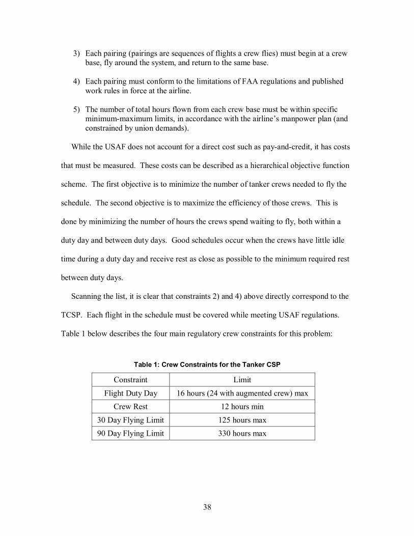
5) The number of total hours flown from each crew base must be within specific minimum-maximum limits, in accordance with the airline’s manpower plan (and constrained by union demands).

While the USAF does not account for a direct cost such as pay-and-credit, it has costs

that must be measured. These costs can be described as a hierarchical objective function

scheme. The first objective is to minimize the number of tanker crews needed to fly the

schedule. The second objective is to maximize the efficiency of those crews. This is

done by minimizing the number of hours the crews spend waiting to fly, both within a

duty day and between duty days. Good schedules occur when the crews have little idle

time during a duty day and receive rest as close as possible to the minimum required rest

between duty days.

Scanning the list, it is clear that constraints 2) and 4) above directly correspond to the

TCSP. Each flight in the schedule must be covered while meeting USAF regulations.

Table 1 below describes the four main regulatory crew constraints for this problem:

Table 1: Crew Constraints for the Tanker CSP

Constraint Limit

Flight Duty Day 16 hours (24 with augmented crew) max Crew Rest 12 hours min

30 Day Flying Limit 125 hours max 90 Day Flying Limit 330 hours max

39

An augmented crew involves two operational crews assigned to a particular flight(s),

thus sharing the flying time. It extends the maximum duty day for each crew by 8 hours.

Crew rest is simply the minimum amount of time a crew needs to be inactive between

duty periods. The 30 and 90 day flying limits represent the maximum number of hours a

crew can fly during those time periods. Since crews enter an operation with a flying

history, these histories must be considered when creating a current crew schedule.

Constraint 3) is overly restrictive for the TCSP. In fact, relaxing it allows us to

explore the strategic prepositioning of crews, especially once operations leave the

deployment phase of a conflict and enter intra-theater operations. Prepositioning crews at

bases other than the aircraft home bases allows the search to find better crew rotations by

allowing one crew to deboard a tanker and rest while another crew continues the mission.

Allowing crews to deboard one aircraft and take off with another creates an additional

constraint within our TCSP. Clearly, a minimum time is needed for crews to leave one

aircraft and operate another. Even if crews land and take off with the same aircraft, there

exists some minimum time to taxi along the runway between flights. This is modeled by

adding a minimum waiting time between flights (MWBF) constraint to the TCSP. Since

no MWBF exists in USAF regulations, these values must be defined by the tanker crew

analyst/scheduler using the ATS metaheuristic.

The final constraint added to the model involves simple geography. If a crew arrives

at base A, it must also depart from base A. To do otherwise is physically impossible.

Finally, the TCSP is not constrained by 5) above. Instead, the tabu search solution

provides the distribution of crew hours needed at each base to cover the flight schedule.

In conclusion, the TCSP can be described as follows:

40

1) Minimize the number of crews required and maximize the efficiency of the crews, subject to constraints 2-7 below.

2) Each flight of the aerial refueling problem must be flown uniquely.

3) Crew duty days must not exceed 16 hours. 4) Once their duty day is over, a crew must rest for a minimum of 12 hours.

5) Crews can fly no more than 125 hours in 30 days and 330 hours in 90 days.

6) The user-defined MWBF must be met. 7) Bases of arrival and departure must match for each crew and aircraft.

4.2 Components of the Adaptive Tabu Search

This section describes the components of the adaptive tabu search (ATS) approach

used to solve the TCSP. It discusses the solution structure for the TCSP, the heuristic

that provides the initial solution, the moves used for the local search process, the

methodology used to evaluate those moves, and the tabu lists used to overcome the trap

of local optimality. These components comprise the elements needed to use Harder’s

OpenTS tabu search framework and Wiley’s group theory code; the backbone of the

JavaTM code developed in this research (Harder, 2002; Wiley, 2000).

4.2.1 Solution Structure.

The cyclic form of the Sn provides a compact solution structure for the TCSP. A

TCSP solution is written as the product of disjoint cyclic factors, where each disjoint

cycle is a single crew’s rotation. The first letter in each cycle is the identification number

of the crew, and each remaining letter in a cycle represents the flights flown and the order

in which they must be flown.

41

For example, assume 5 tanker flights must be flown and there exist 5 crews to fly

them. By mapping letters 1-5 to crews 1-5, mapping the letters 6-10 to the five flights,

and working within S10, each flight must be flown once, satisfying constraint 2) above.

Some representative solutions taken from S10 that cover each flight once are:

(1,6,7,8)(2,9,10), (1,6,7,8 9,10), and (1,6)(2,7)(3,8)(4,9)(5,10).

Reexamine what each disjoint cyclic factor in the solutions above represents. They

are the flights covered by each tanker crew in the solution. For example, (1,6,7,8)(2,9,

10) means crew 1 covers flights 6-8, crew 2 covers flights 9-10, and crews 3-5 are

unassigned or inactive. It is also clear that crew 1 must fly flight 6, then flight 7, and

finally, flight 8.

Various components of our adaptive tabu search use long-term frequency information

to perform their individual operations. As the size of the problems grow, storing and

comparing information on crew rotations, solutions, or conjugacy classes becomes

computationally expensive. A typical solution to this problem is to create hashing

functions that map each crew rotation, complete solution, or conjugacy class to integer

values (Glover and Laguna, 1997:246). These hashing functions are used to store the

frequency information on the various items in hash maps. Sections 4.2.1.1-4.2.1.3

describe the hash functions developed for various components of our solution structure.

4.2.1.1 Rotation (Cycle) Hash Function.

The rotation or cycle hash function is used to capture attributive information on each

individual crew rotation. This allows the search to operate on partial solutions and is

42

specifically used in the vocabulary building conducted by the set partitioning optimizer

described in Section 4.3.

Examine the hash calculation of a member of S10 as described above. The process

begins by generating randhash, an n-sized vector of unique random integers uniformly

ranging from 1 to n*n. Each element of randhash maps a random integer to one of the

original n letters. In the case of S10, randhash has 10 unique elements randomly

generated from the U(1,100) distribution. Given a crew rotation or disjoint cycle d with

m elements, define the hashing function as follows:

Equation 2: Hashing Function for a Crew Rotation

. cycle of position in foundletter theis where,][ 1diddrandhashh i

m

i id ∏ ==

For example, suppose we have randhash = [2,51,11,24,74,43,19,15,60,9] and d = (1 6

7 8). The resulting hash value is calculated as hd = 2*43*19*15 = 24510.

It is clear that hd is specific to the TCSP because it does not account for the ordering

of the elements within d. This is sufficient for the TCSP because of the manner in which

the letters are assigned, the departure time ordering of the input flight schedule, and the

candidate list strategies used to build the neighborhoods in Section 4.2.3. Collisions

occur when two different rotations are mapped to the same hash value. The ATS

explicitly avoids collisions between cycles such as (1,6,7,8), (1,6,8,7), (1,7,6,8), (1,8,6,7),

and (1,8,7,6) by using candidate list strategies to disallow solutions such as the last four

because of inappropriate departure time sequencing.

While hd is specific to our problem, it is possible to slightly modify the methodology

and create a generalized form for hd. This generalized form is useful in solving

combinatorial optimization problems where within-cycle ordering matters. Start by

43

generating randhash, an n x n-sized array of unique random integers uniformly ranging

from 1 to 2* n2. Each element of randhash maps the arc i-j in a disjoint cycle. For

example, for the disjoint cycle (1 6 7 8), randhash[1][6] is the random integer

representing the arc 1-6 in the cycle. The trivial inactive crews such as (3) are mapped to

elements randhash[i][i]. For S10, randhash has 100 unique elements from the U(1,200)

distribution.

Given a crew rotation or disjoint cycle d with m elements, we define the generalized

hashing function as follows:

Equation 3: General Hashing Function for Disjoint Cycles

letter.first the to inletter last thefrom arc theis ]1][[ and cycle of

position in foundletter theis where],[ ][]1][[ 11

1

dmrandhashd

idddrandhashmrandhashh iim

i id +−

=∏∗=

One obvious disadvantage with Equation 3 versus Equation 2 is the storage

requirements for randhash. In Equation 3 the storage requirement is O(n2), while it is

only O(n) for Equation 2.

4.2.1.2 Solution Hash Function. The importance of the solution hash function to the ATS cannot be overemphasized.

It is used for comparisons within the tabu list and helps drive much of the adaptive

scheme throughout the search. This said, a simple extension of the rotation hash function

works extremely well for the TCSP. Suppose solution s exists with c disjoint cycles or

crew rotations. The solution hash function is defined as follows:

44

Equation 4: Solution Hashing Function for the TCSP

above. 2Equation in defined is where,1 d

c

d ds hhh ∑ ==

If a generalized solution hash function is required for a different application, simply

modify Equation 4 by using the hd defined in Equation 3. Since the symmetric group

theory code used to build the ATS contains a method to calculate hash values for group

elements, it appears useful to compare the new hash function to it. Table 2 below

displays the results of the comparison:

Table 2: Comparison of generalized hs and the existing group theory hash function n Size of Sn Collisions with group

theory hash function Collisions with

hs Cum time to calculate with group theory hash (milliseconds)

Cum time to calculate hs (milliseconds)

3 6 0 0 0 0 4 24 0 0 0 0 5 120 1 0 0 0 6 720 11 0 0 0 7 5040 555 4 47 16 8 40320 9801 35 153 109

Table 2 clearly shows hs outperforms the existing group element hash function. Not

only does it significantly reduce the number of collisions, but it calculates the hash value

in less time.

4.2.1.3 Conjugacy Class Hash Function.

Knowing the conjugacy class of a solution may prove useful to general tabu search

methodologies. Intensification or diversification schemes may be driven by long term

conjugacy class frequency information. In our TCSP application, conjugacy class

frequency information was used for two purposes. During ATS development, it was used

45

to determine if the search was achieving suitable diversification. This conjugacy class

information, recorded using the conjugacy class hash function below, spurred changes

that improved the flow of the ATS. In Chapter VI, this conjugacy class information is

used to measure the degree of diversification achieved by the ATS.

To gather conjugacy class frequency information, it is useful to use a hashing function

as seen with rotations and solutions above. The conjugacy class hash function is based

on the typical notation for a conjugacy class:

2).:1991 (Sagan,solution in the length of cycles ofnumber theis where, ... ...21 21 kmnk kmmmm nk

For example, the solution (1 6 7 8)(2 9 10) above (remember it contains 5 crews) is in the

conjugacy class 133141.

Given the conjugacy class notation, we define the conjugacy class hash function as

follows:

Equation 5: Conjugacy Class Hash Function

solution. in the sizes cycledistinct ofnumber theis and

and ofion concatenat theis )(. where),(.1

r

mkmconcatkmconcatkhiii kikik

r

i iCC ∏ ==

Therefore, the hash value of the conjugacy class 133141 above is 13*31*41 = 16523.

4.2.1.4 Characterizing the TCSP Solution.

To adapt various parameters during the search, it is useful to characterize a TCSP

solution in terms of feasibility. Section 4.2.1 concludes by defining three types of

feasibility measures: feasible, near feasible, and poor infeasible.

Feasible solutions are those solutions that meet all TCSP constraints. These are risk

free solutions for the decision maker, i.e., all USAF regulations are satisfied.

46

Near feasible solutions violate some of the constraints, but the amount of constraint

violation is within an acceptable tolerance. By examining and recording near feasible

solutions, a decision maker may examine the risks of relaxing constraints such as crew

rest. The size of each constraint deviation is user-defined and preset prior to starting the

solver.

Finally, a poor infeasible solution exceeds the allowable constraint violation on one or

more of the TCSP constraints. These are solutions that exceed at least one of a decision

maker’s acceptable tolerances.

The solution structure has been discussed, three useful hashing functions have been

developed, and TCSP solutions have been characterized. The next section discusses the

heuristic that provides a starting point for the ATS.

4.2.2 Initial Solution Construction.

The first task in starting the tabu search is creating an initial solution. The heuristic

used is very similar to the Crew Dog tool used by AMC analysts today and is clearly

suboptimal. This research uses a global tabu search approach to find better solutions.

Figure 5 below displays the flow of the process.

The tabu search runs in two modes: analysis or operational. The analysis mode

allows AMC analysts to study questions such as, “What is the proper crew ratio for a

given scenario and how does the structure of the schedule affect this?” The operational

mode assumes that AMC crews are physically mobilized for a deployment or other

operation. It searches the solution space to find extremely good flight assignments for

these crews. Each mode considers all crew constraints as defined in Section 4.1.

47

The only component of the ATS affected by these two modes is the initial solution

heuristic. Once an initial solution is constructed, the tabu search operates identically for

each mode.

In analysis mode, the heuristic assumes it is given an aircraft schedule sorted in order

of increasing flight departure, i.e., the first flight in the list departs the earliest. The

heuristic then creates an initial crew and populates its 30 and 90 day flying histories in a

JavaTM array list. The flying histories are populated using two monte carlo draws. The

first uses a user-supplied input parameter, probfly, to determine whether or not a crew

flew on any of its previous 90 days. If a crew did fly, then another draw is made and

compared to the cumulative flying time distribution in the AMC furnished

crewProbabilities.txt file to determine the flight duration. The probfly and

crewProbabilities.txt allow an analyst to study how historical operations tempo affects

current warfighting.

Once the first crew is created, the heuristic begins to iterate through each flight in the

schedule. For each flight, it examines each crew by order of creation. It checks all

constraints and determines if a crew can feasibly cover the flight. If so, the heuristic

assigns the flight to the crew with the smallest identification number. Otherwise, the

heuristic creates a new crew, populates the 30 and 90 day flying histories, and determines

whether or not the new crew can cover the flight. New crews are created until all flights

in the aircraft schedule are covered. The heuristic ensures an initial feasible solution

when running the tabu search in analysis mode.

The operational mode heuristic is slightly different. It assumes the same type of flight

schedule as described above, but it also assumes the existence of a crewHistory.txt file.

48

This file contains the 30 and 90 day flying histories of each mobilized crew. Instead of

creating crews on the fly, the heuristic immediately instantiates the given number of

crews and reads their crew histories from the text file.

Figure 5: Initial Solution Heuristic

What is the mode of the search?

OperationalAnalysis

Read ordered air refueling

schedule

Create 1st crew and populate 30/90

histories

Can next flight be placed in existing

crew rotation?

Add flight to 1st feasible

crew rotation

Create new crew and populate 30/90

histories

Read ordered air refueling

schedule

Create all crews and read all 30/90

histories from file

Can next flight be placed in existing

crew rotation?

Add flight to 1st feasible crew

rotation

Does the arrival base of last flight in

any crew rotation match the departure base of flight being

assigned?

Yes

No

Yes

No

No

Place flight in rotation of crew 1

Add flight to first crew rotation with

matched bases

Yes

Are there flights left to be assigned?

Terminate

No

Yes Are there flights left

to be assigned?

Terminate

No

Yes

49

The heuristic then begins iterating through the flights. For each flight, the heuristic

checks the TCSP constraints and determines if one of the existing crews can cover it. If

so, the flight is assigned to the crew with the smallest identification number. If not, it is

clear that the initial solution is infeasible. It then ignores every constraint other than

matching the arrival and departure bases. It assigns the flight to the crew with the

smallest identification number whose last arrival base matches the flight’s departure base.

If no arrival-departure base matches are available, the heuristic places the flight in the

rotation of crew one. If this occurs, the initial solution contains a physical dislocation

and becomes severely infeasible.

Once an initial solution is built, the tabu search must examine its neighborhood to

determine the next incumbent solution. The next section discusses the neighborhoods

built within the ATS, as well as the candidate list strategies used to restrict the

neighborhood size.

4.2.3 Restricted Neighborhood Construction.

The local search examines the current neighborhood of an incumbent solution, and

chooses a move to a different solution. This section defines the moves used to create the

neighborhood structure.

For scheduling problems, it is well known that good tabu search algorithms have been

developed using swap and insert moves (Barnes, et al., 1995; Lourenco, et al., 1998;

O’Rourke, et al., 2001; Wiley, 2001). For the TCSP, a swap is defined as exchanging

50

flights in two crew’s rotations and an insert is defined as taking a flight from one crew’s

rotation and placing it in another crew’s rotation.

As problem size increases, individual swap and insert neighborhoods can become

excessively large. For example, the complete swap neighborhood for 1000 flights

consists of 1000(999)/2 = 499,500 members. This research used a TCSP specific

candidate list strategy to reduce neighborhoods of this size. The ATS uses the following

restrictions to create its Restricted Swap Neighborhood:

1) Only swap flights between disjoint cycles or rotations.

2) Only swap flights that maintain proper base of arrival-departure matching. 3) Only swap flights that maintain increasing letter order within each affected

rotation. Given the time-sequenced nature of the TCSP, it does not make sense to swap flights

within a crew’s rotation. Doing so creates a situation where a crew’s departure for one

flight occurs later than the departure time for a subsequent flight in its rotation. For

example, in the solution (1,3,4,6)(2,5,7,8), it is not realistic to swap flights 4 and 6 to

obtain (1,3,6,4)(2,5,7,8) because it violates departure time sequencing.

Swap restriction 2) ensures that crews are physically able to fly the given rotations.

Swap restriction 3) is similar to 1) in that it avoids inappropriate time sequencing in the

rotations. Unlike 1), swaps between two disjoint cycles are examined to determine if a

poor sequencing results. Let us return to the solution (1,3,4,6)(2,5,7,8). Exchanging

flights 4 and 8 results in the solution (1,3,8,6)(2,5,7,4). Clearly, both crews now have

inappropriate time-sequenced rotations.

51

Similarly, the Restricted Insert Neighborhood is created using the following

restrictions:

1) Only insert a flight from one crew rotation to another. 2) Only allow inserts that maintain proper base of arrival-departure matching.

3) Only allow inserts that maintain increasing letter order within each affected

rotation. Allowing inserts within cycles creates the same sequencing problem as the within

cycle swaps described above. Insert restriction 2) maintains geographical feasibility.

Insert restriction 3) is similar to the swap restriction as well. Given (1,3,4,6)(2,5,7,8), the

search disallows inserting flight 7 in front of 4 to create (1,3,7,4,6)(2,5,8) because it

creates inappropriate departure time sequencing for the first crew.

With the Restricted Swap and Insert Neighborhoods created, it may appear enticing to

use them sequentially, i.e., use an insert to take us to a different solution, and then

explore the solution’s conjugacy class with the swap neighborhood. But previous tabu

search methods have demonstrated better performance by examining the neighborhoods

simultaneously (Barnes, et al., 1995). Therefore, the ATS uses a Combined Restricted

Swap/Insert neighborhood (CRSIN).

The ATS can periodically become trapped in areas of poor infeasibility during the

search process. The ATS responds to this situation by changing the structure of the

CRSIN described above. It does this in two ways. First, it allows mismatches between

arrival and departure bases. Second, the neighborhood targets the crews that are

currently infeasible. We call this neighborhood the Targeted Combined Restricted Swap-

Insert Neighborhood (TCRSIN). The TCRSIN is vital for escaping the trap of poor

52

infeasibility. Once the ATS determines the solution trajectory is trapped in poor

infeasibility, as explained in Section 4.4.2, it uses the TCRSIN until, at a minimum, near

feasibility is restored.

Once the CRSIN or TCRSIN is built, the next move cannot be chosen until all

members of each neighborhood are evaluated. The next section describes the adaptive

methodology used to evaluate each neighborhood move.

4.2.4 Solution and Move Evaluation. This section describes how individual solutions and solution/move pairs are evaluated

during the ATS. It begins by discussing the evaluation of individual TCSP solutions and

solution/move pairs. It then details the scheme used to adapt the evaluation function’s

numerous penalty weights. It concludes by describing the methodology used to calculate

the penalties for the TCSP constraints.

To evaluate the initial solution or a solution generated from a restart, Equation 6 is

used:

Equation 6: Solution Evaluation

) () (

) ()() () () (#

90

30

penaltiesbasemismatchedpenaltiesdayninety

penaltiesdaythirtyMTBFpenaltiesdaydutypenaltiesrestcrewstimewaitingeval

bases

MTBFduty

restcrewssolution

∗+∗+

∗+∗+∗+∗+∗+=

ρρρρρ

ρρ

Notice that the evaluation function clearly captures the objectives and constraints that

compose the TCSP: a crew variable to capture the number of crews in the solution, a

waiting time variable to capture a measure of the efficiency of the schedule, and penalty

variables relating to violations of each TCSP constraint.

53

With the swap and insert moves used, only two crews are affected at any iteration of

the search. Therefore, instead of using Equation 6 for each move evaluation, the ATS

uses a well-known incremental means of evaluating moves. First, the ATS calculates the

difference in the number of crews between the incumbent solution and the solution

created by the move. It isolates the two crews affected by the move, and calculates the

differences in each remaining variable for those crews alone. Of course, the crew waiting

time and constraint penalties must be stored and updated each iteration.

The resulting move evaluation function is as follows:

Equation 7: Move evaluation

) () (

) ()() () () (#

90

30

penaltiesbasemismatchedpenaltiesdayninety

penaltiesdaythirtyMTBFpenaltiesdaydutypenaltiesrestcrewstimewaitingeval

bases

MTBFduty

restcrewsmove

∆∗+∆∗+

∆∗+∆∗+∆∗+∆∗+∆∗+∆=

ρρρρρ

ρρ

Given evalmove, OpenTS uses the following criteria to choose a move:

1) Choose the move with the smallest evaluation value, to include an unimproving move.

2) If two move values are equal, choose the move occurring first in the neighborhood.

Equations 6 and 7 contain seven penalty parameters that the ATS must continuously

adapt. These parameters allow the ATS to control its strategic oscillation between the

feasible, near feasible, and poor infeasible areas of the solution space. The ATS

implements the self-adjusting scheme proposed by Gendreau, et al. (1996) and used

successfully by O’Rourke, et al. (2001). This research shows the scheme can

successfully control a significantly larger number of parameters, nearly four times the

number of penalties adjusted for O’Rourke’s vehicle routing problems. Each of the

54

penalty parameters described in Equations 6 and 7 are independently adjusted every five

iterations as follows:

Equation 8: Penalty parameter adjustment

.,..., where,2 15/ basesrestcrewsipenaltyii =∗→ −ρρ

The value of penalty in Equation 8 varies depending on the parameter being adjusted.

For ρcrews, penalty is the number of feasible or near feasible solutions in the last ten

iterations. Therefore, if the last ten iterations have all been feasible or near feasible

solutions, ρcrews doubles and induces the search to move to smaller crew solutions. If the

last ten iterations have all produced poor infeasible solutions, the value of ρcrews is halved

and the search moves towards solutions with a larger number of crews.

For the parameters relating to the TCSP constraints, penalty refers to the number of i

infeasible solutions found in the last ten iterations, i.e., for i = rest, the number of

infeasible solutions that violated crew rest. As with the ρcrews, if constraint i is violated

during each of the last ten iterations, ρi doubles and provides an incentive for the

constraint to be satisfied. Likewise, ρi halves if i was not violated during the last ten

iterations. When the violation counts are greater than zero and less than ten, the search

adjusts the penalty between ½ and 2 times the current penalty.

A description of the method used to quantify the number of active crews and

constraint penalties found in Equations 6 and 7 concludes this section. When evaluating

a complete solution, the ATS simply counts the number of nontrivial disjoint cycles in

the group element and records this value as the number of active crews in the solution.

When determining the number of active crews created by a move, the ATS first checks

55

the type of move evaluated. If the move is a swap, the ATS recognizes that conjugation

maintains the number of active crews. If the move is an insert, one of three cases may

arise and the ATS recognizes such:

1) The insert leaves the number of active crews the same. 2) The insert takes the only assigned flight from one active crew and places it in

another crew’s rotation. This deactivates the crew that lost the flight and reduces the number of active crews by one.

3) The insert takes a flight from an active crew with multiple flights and places it in

a previously inactive crew’s rotation. This activates the crew and increases the number of active crews by one.

When evaluating a complete solution, the ATS first initializes a penalty array for each

constraint. It then performs the linear operation described in Figure 6 to calculate and

record penalties for each constraint and each crew. For each constraint, the crews’

penalties are summed for use in Equation 6. For subsequent move evaluations, the linear

operation is performed for the two crews affected by the move and the crews’ recorded

penalty information is used to calculate the differences found in Equation 7.

A simple example is now used to describe the algorithm displayed in Figure 6.

Assume crew 0 covers flights 1-4, so the crew rotation is (0,1,2,3,4). The ATS first

penalizes the solution for any 30 or 90-day flying history violations, as described below.

It initializes the first flight in the rotation and first flight in the duty day to flight 1.

The ATS assumes the schedule starts with the initial briefing that occurs before the

schedule’s first flight departure. The briefing length is a user-defined value, set to forty-

five minutes for this research. The time between the departure of flight 1 and the

schedule’s start time is added to crew 0’s waiting time. In this case, flight 1 is the first

flight in the schedule so no waiting time would be added. If more flights exist, the flight

56

to examine is incremented by one. In this case, flight 2 is the next flight to examine. The

waiting time from the arrival of flight 1 to the departure of flight 2 is added to crew 0’s

waiting time array. The ATS then determines if the minimum wait time between flights 1

and 2 is satisfied, linearly penalizing if necessary. Linear penalties are used for every

constraint and calculated as such:

Equation 9: Linear Penalties for TCSP Constraints

required. are hours 12 states constraintrest theand flights obetween twrest hours 11 calculatemay algorithm theexample,for ;constraint particular theof lue target va theis esired and

algorithm by the calculated value theis where,| - | =valued

valueactualvaluedesiredvalueactualpenalty

After checking the MWBF constraint, the ATS determines if the departure base of

flight 2 matches the arrival base of flight 1. If the bases are different, a penalty of 1 is

added to crew 0’s mismatched base penalty array. Notice that while MWBF is described

in time units, the mismatched bases penalty is a binary, unitless value that simply states

whether or not a mismatch occurred. The adaptive penalty scheme previously described

allows the smooth integration of these two types of penalties.

Next, the ATS determines if the minimum amount of rest occurs between flights 1 and

2. If sufficient rest exists, the examined flight is set as the start of the next duty day and

the next existing flight is set as the flight to examine. In this case, the ATS sets flight 2

as the first flight in the next duty day and sets flight 3 as the flight to examine. If

insufficient rest exists, the ATS checks the duty day constraint.

The length of the duty day is calculated between the first flight in the duty day, in this

case flight 1, and the arrival flight being examined, in this case flight 2. If the duty day

constraint is satisfied, the ATS increments the flight to examine by one and restarts the

57

process at the waiting time calculation. In this case, the flight to examine would be

incremented to 3 while the first flight in the duty day remained 1. If the duty day

constraint is violated, the ATS performs a local optimization by determining the

minimum of the proposed rest and duty day penalties. In developing the ATS, we found

the following reasons to integrate this local optimization within the algorithm:

1) If both constraints are penalized, the solution is unduly penalized and the search fails to seek solutions with a smaller number of crews.

2) The particular constraint penalized drives the duty day flow, as we describe now.

Suppose the ATS determines crew rest is the least violated constraint. The ATS then

flows to a new duty day and sets the flight being examined, in this case 2, as the first

flight in that duty day. The flight to examine is set to flight 3, and the ATS restarts

processing the constraint penalties.

Suppose the ATS determines duty day length is the least violated constraint. In this

case, the ATS completes the existing duty day with the flight being examined, i.e.,

completes the duty day with flight 2, and starts a new duty day with the next existing

flight, flight 3. The algorithm records the waiting time between the departure of the first

flight in the next duty day and the arrival of the last flight examined. It must also check

all constraints but the duty day constraint. In this case, the waiting time between flights 2

and 3 is recorded and all constraints but the duty day constraint are checked. This flow is

seen in the lower right hand corner of Figure 6. With this complete, the ATS sets the

flight to examine as the next existing flight, i.e., flight 4, and restarts the process.

58

Figure 6: Evaluation of a Single Crew

Reset 1st duty day to f

Set flight to examine to f, first flight in duty day to f, and add waiting time from start time to

departure time f

Set next flight to examine, f →f+1, if any remain.

Add waiting time between f and f-1

Penalize MTBF violation between f and f-1

Penalize mismatched

arrival/departure bases for f and f-1

Is rest constraint satisfied?

Is duty constraint satisfied?

Penalize min(rest penalty, duty penalty)

Was rest penalized? Reset 1st duty day and f → f+1

Add waiting time between f and f-1.

Penalize MTBF for f and f-1.

Penalize mismatched bases

for f and f-1.

Penalize rest violation between f

and f-1.

Penalize 30/90 day flying histories

Yes

No

Yes

No

Yes No

59

In Figure 6, notice the ATS calculates the 30 and 90 day flying history penalties

before starting its loop to determine the remaining penalties. The calculation of the

history penalties is another operation approached separately. While calculating the other

penalties, the ATS kept track of the rest and duty day structure of the crew rotation.

When calculating the flying history penalties, the ATS must track the 30 and 90 calendar

day windows.

The approach to the problem is straightforward. To evaluate the crew’s rotation, the

flying history array list is updated to recognize additional flying time and recognize the

passing of time. Whenever the algorithm transitions to a new calendar day, it determines

whether or not to penalize the 30 or 90-day flying history constraints. There is one

exception to this rule. When there are idle days between flights, the ATS does not

attempt to penalize the histories as the array list transitions. Idle days added to the 30 or

90-day history cannot create either constraint violation, and the ATS would double

penalize for previous flights if it checked the histories again.

The logic required to implement the approach is presented below, and its discussion is

broken into two parts: calculation of the 30 and 90-day flying history penalties for the

first flight and calculation of the 30 and 90-day flying history penalties for all remaining

flights.

Figure 7 displays the process used to calculate the 30 and 90-day flying histories for

the first assigned flight. First, the flying history array list is updated to account for idle

time between the schedule start time and the departure time of the first flight in the

crew’s rotation. For example, if there are three idle days before the crew starts its

60

rotation, the top three elements of the array list are removed and three flying days of zero

are added to the end of the list.

The second step determines if the first flight departs and arrives on the same day. If

so, it removes the first member in the list and adds the first flight time to the bottom.

If no other flights exist in the rotation, penalties for the 30 and 90-day flying histories are

calculated and the algorithm terminates. If other flights exist, the ATS moves to examine

the next flight in the rotation.

If the first flight’s departure and arrival days are different, a separate sequence of

events occurs. First, the ATS removes the top member of the array list and adds the

flying time occurring on the day of departure to the bottom of the list. Since the

algorithm removed a day from the history list and added the most recent day, it checks

the crew history and calculates history penalties. The ATS removes the top member of

the list again and adds the flying time occurring on the day of arrival to the bottom of the

list. At this point, the ATS makes another decision. If no other flights exist in the

rotation, it calculates history penalties and the algorithm terminates. If other flights exist,

history penalties are not calculated because the flying day may not be finished. The ATS

simply moves to examine the next flight in the rotation.

61

Figure 7: Evaluation of 30/90 Day Flying History for First Flight

Initialize flight to examine to initial flight, f = 1

Update history list for idle days from start time to f’s

departure day

Does departure day of f = arrival day of f?

Remove day 1 from history list. Add time from dep

time f to 0000 to end of list.

Calculate 30/90 day flying history penalties

Remove day 1 from history list. Add time from 0000 to

arr time f to end of list.

Is crew rotation complete?

Calculate 30/90 day flying history penalties

Set f → f + 1 and terminate.

Remove day 1 from history list. Add flight time of f to

end of list.

Is crew rotation complete?

Calculate 30/90 day flying history penalties

Yes

No

Yes

Yes

No

No

62

Figure 8 below displays the logic used to evaluate the remainder of the crew’s flights.

The ATS first determines if the previous flight arrives on the same day the current flight

departs. If not, the flying day previously left open is complete and history penalties are

calculated. The history list is updated for idle days between the previous flight’s arrival

and the current flight’s departure. Once the list is updated for idle days, the logic is

identical to that described for the first flight.

If the previous flight’s arrival day and the current flight’s departure day are identical,

the logic changes. The ATS first determines if the current flight’s departure and arrival

days are the same. If they are, the current flight is completed on the same day the

previous flight finished. Therefore, no days are added to or removed from the history list.

The current flight time is simply added to the flying time of the last day on the history

list. If the current flight completes the rotation, history penalties are calculated and this

part of the algorithm terminates. If not, the ATS returns to evaluate the next flight in the

rotation.

If the current flight’s departure and arrival days are different, the ATS first updates the

last day in the history list by adding the flying time occurring during the current flight’s

departure day. Note, the top member of the history list is not removed because the

current flight’s departure day flying time occurs on the same day as the previous flight’s

arrival. Once this update occurs, the ATS calculates history penalties. It removes the

first member of the history list and adds the current flight’s arrival day flying time to the

end of the list. If the crew rotation is complete, the history penalties are calculated and

this part of the algorithm terminates. If other flights exist, the ATS returns and evaluates

the next flight in the rotation.

63

Figure 8: Evaluation of 30/90 Day Flying History for Other Flights

Update history list for idle days from arr f-1 to dep f

Does arrival day of f-1 = departure day of f?

Update last day on list with time from dep to 0000 to end of list.

Calculate 30/90 day flying history penalties

Remove day 1 from history list. Add timefrom 0000 to arr time f to end of list.

Is crew rotation complete?

Is crew rotation complete?

Calculate 30/90 day flying history penalties

Set f → f + 1

Does departure day of f = arrival day of f?

Calculate 30/90 day flying history penalties

Update last day on list with flight time of f

Calculate 30/90 day flying history penalties

No

Yes

Yes

No

Yes

Yes

No

NoDoes departure day of f = arrival day of f?

Remove day 1 from history list. Add time from dep f to 0000 to end of list.

Calculate 30/90 day flying history penalties

Remove day 1 from history list. Add flight time of f to end of list.

No

Yes

64

4.2.5 Tabu List.

Now that a procedure exists to calculate solution and move values, this section

describes the tabu lists created for the ATS. Recall that tabu search uses tabu lists to

avoid becoming trapped at local optimum.

The ATS uses a solution-based tabu list. The search records the hash value of each

solution visited in a JavaTM array list. The tabu tenure is implemented in two ways. The

statistical analysis in Chapter VI provides a comparison of their utility.

The first approach makes every solution visited tabu for the rest of the search. Morton

and Pentico (1993) suggest this tenure is robust for a wide variety of scheduling

problems. This is simple to implement, but it may significantly restrict the tabu search

and may be computationally expensive.

This implementation restricts the search because of its interaction with the move

evaluation function previously described. Suppose the ATS arrives at solution x, at

iteration 100, with a set of penalty weights as defined in Section 4.2.4. If the ATS

allowed a return to solution x at iteration 1000, the penalty weights would likely be

different and could possibly send the trajectory into a part of the solution space superior

to the area originally visited from x. Making all previously visited solutions tabu would

prevent x from being revisited, and could restrict the tabu search.

An adaptive tabu tenure is the second scheme studied in this research. Assume the

tabu tenure at a particular iteration is t. The ATS searches the last t elements of the array

list previously described to determine tabu status. The ATS adapts the tenure using the

following rules:

1) If the current solution is a revisited solution, the tabu tenure doubles.

65

2) If the current solution is unique, the tenure decreases by one.

Rule one should allow the search to quickly escape cycling and provides a

diversification mechanism for the search. Rule two should provide a means to reduce the

severe tabu restriction of a long list when cycling ceases.

4.3 Vocabulary Building With Set Partitioning

This research extends the heuristic/post-optimization approach discussed in Section

2.1.2 by developing an integrated tabu search/SPP optimizer. This section describes the

SPP portion of the optimizer, while the next section describes how the SPP optimization

is embedded within the overall tabu search scheme.

Figure 9: Typical Local Search Figure 9 displays the typical flow of a local search algorithm. From an incumbent

solution, a neighborhood of solutions is built and evaluated, with a new incumbent

solution chosen from the neighborhood.

Kelly and Xu note that some of their heuristic solutions to the VRP are infeasible, but

these infeasible solutions contain good partial solutions that should be included in the

pool of columns sent to the SPP optimizer (Kelly and Xu, 1998:4). This research extends

Incumbent Solution

Build neighborhood of solutions

Evaluate neighbor solutions

66

this idea by developing a pool that contains good partial solutions from the initial solution

and good partial solutions from the series of created neighborhoods.

Figure 10: ATS Local Search

Figure 10 shows the ATS method for collecting partial solutions. To initialize the pool,

all the feasible or near feasible crew rotations from the ATS initial solution are added to a

JavaTM hashmap that stores their hash value as the key and a rotation/waiting time pair as

the value. Near feasible rotations may initially occur when no feasible starting solution

exists for a problem solved in the operational mode.

Once the pool is initialized with the individual crew rotations from the starting

solution, crew rotations may be added with each neighborhood move evaluation. Since

the neighborhoods created within this research consist of swaps and inserts, only two

crews are affected by any move. If the crew rotations of either affected crew are feasible

or near feasible partial solutions, and the partial solutions have not been previously

recorded, the hashmap is updated with the appropriate rotation/waiting time pair.

Incumbent Solution

Build neighborhood of solutions

Evaluate neighbor solutions

Record feasible and near feasible partial solutions of neighbor solutions

67

At various times during the search, the ATS solves a near feasible or feasible SPP

using the Java Concert Technology embedded within ILOG CPLEX 7.5. The near

feasible SPP contains crew rotations that are both feasible and near feasible. The feasible

SPP has columns whose crew rotations are all feasible. This ensures the solution created

by solving a feasible SPP is itself feasible. The next section describes exactly when the

ATS chooses to solve the two types of problems. The SPP was defined in Equation 1. In

this case, the waiting time of each rotation represents its cost coefficient. There are two

reasons for using waiting time despite its minimization being the ATS’s secondary

objective:

1) Solving a SPP that minimizes the number of active crews causes the ATS to converge prematurely to poor solutions. These solutions characteristically have poor waiting times AND an unnecessarily large number of active crews.

2) Feasible solutions often occur in the vicinity of near feasible solutions.

Minimizing waiting times moves the search to near feasible solutions with increasingly fewer active crews. The tabu search itself finds smaller-crewed feasible solutions near these infeasible solutions. The ATS uses the SPP optimizer to vocabulary build. The SPP’s main role is to provide the ATS with excellent points at which to restart the search.

Finally, note that many of the SPP problems the ATS creates are too large for CPLEX

to efficiently solve. In some cases, the solution time for CPLEX either overwhelms the

overall search time or CPLEX runs out of memory and fails to report a feasible answer.

Therefore, the ATS actually uses CPLEX in a heuristic manner. It places a ten-minute

threshold on the SPP solution process. If an optimal solution is not found in ten minutes,

CPLEX reports the best solution found so far.

68

4.4 Completing the ATS Framework

With the discussion of the components of the ATS and SPP optimizer complete, this

section completes the chapter by describing how the overall tabu search process

functions. The first section describes an iteration of the adaptive tabu search, as driven

by Harder’s OpenTS software (2002). The second section discusses the first variant of

the ATS, an adaptive search that includes an intensification scheme. The final section

completes the chapter by discussing the integrated ATS/SPP optimizer.

4.4.1 One Iteration of the ATS.

Figure 11 below displays an iteration of the OpenTS tabu search framework (Harder,

2002). This basic sequence is repeated throughout the ATS process, except in the special

case where the SPP optimizer completes the iteration. It is important to note that the

OpenTS architecture provides none of the fundamental methods needed to solve a TCSP.

All the methods described in Section 4.2 were coded independently, and OpenTS simply

provided tabu search bookkeeping services.

The process is as follows: the ATS starts from an initial solution built using the

greedy heuristic of Section 4.2.2. It builds the neighborhood of restricted moves

described by Section 4.2.3. These neighborhoods are adaptive, meaning the

neighborhoods change from iteration to iteration depending on the current incumbent

solution and long-term frequency memory. Once the moves are created, they are sent to

the objective function evaluator. The objective function evaluator uses the methods

described in Section 4.2.4 to evaluate the neighborhood. The best non-tabu move

amongst the moves in the neighborhood is chosen next. The determination of the best

69

move is an adaptive process for the ATS with intensification, and it is described in the

next section. Finally, the move is used to operate on the current solution. If the move is

a swap, the ATS uses conjugation to move to the new current solution. If it is an insert

move, the ATS uses the function composition operator. These are the conjugative and

template-based moves described in Section 2.2.1. With a new incumbent solution found,

the process repeats.

Figure 11: One Iteration of OpenTS (Harder, 2002)

4.4.2 The ATS with Intensification.

This section on ATS with intensification begins by defining the elements that drive the

search process. The ATS maintains two elite lists of size five; one for the best feasible

solutions and one for the best near feasible solutions found throughout the search. The

elements in these elite lists are ordered by number of active crews first and total waiting

time second. Closely related to the elite lists is the counter, ISGS, the number of

iterations since finding a good solution, i.e., the number of iterations since updating either

70

elite list. The second counter used to coordinate the search is CP, the number of

consecutive poor infeasible solutions the ATS visits.

CFIM, choose the first improving move, is the final variable defined. It is a boolean

variable. When its value is true, the first improving move, as described by the move

evaluation, is chosen as the best move. When its value is false, every move in the

neighborhood is evaluated and the best move is chosen. For the ATS with intensification,

the ATS uses CFIM with a true value in the early stages of the search. This is done for

two reasons:

1) At the beginning of the search, the ATS is diversifying and therefore, seeking a larger sampling of the solution space.

2) When insert moves are placed first in the neighborhood and the swaps second, the

likelihood of the first improving move taking the ATS to a smaller-crewed solution increases. The likelihood increases for two reasons. One, only inserts can decrease the number of active crews in a solution. Two, since the inserts are placed first in the neighborhood, the objective function evaluator finds an insert as the first improving move, if one exists, before evaluating any swaps.

Note that these four elements are not the lone drivers of the search space trajectory.

Every five iterations, the search adapts the penalty weights for the solution and move

evaluation equations, as described in Section 4.2.4. In addition, the neighborhoods

themselves adapt to change the search trajectory, as described below.

The first phase of the ATS uses the elite lists, ISGS, CP, CFIM, and CRSIN to

coordinate the search in a straightforward manner. After each iteration, the ATS attempts

to update the elite lists. If either of the lists is updated, the ISGS is reset to zero. If

neither is updated, ISGS increases by one. The ATS also characterizes the solution as

feasible, near feasible, or poor infeasible. If the solution is poor infeasible, CP increases

by one; otherwise, CP is reset to zero. If the search performs a preset number of CP

71

iterations, a value studied in Chapter VI, it identifies the search as trapped in a poor

infeasible space and changes the neighborhood used to the TCRSIN. When the search

returns to a near feasible or feasible solution, it changes the neighborhood back to the

CRSIN.

When ISGS equals its preset limit, another value studied in Chapter VI, phase two

intensification begins. CFIM becomes false, and the ATS evaluates the entire

neighborhood of each incumbent solution. A restart list is then created from each

solution on the elite lists. The ATS starts a new phase one-type search from each

member of the restart list. CFIM remains false for these intensified searches. When

ISGS equals its preset limit during phase two, the next member on the restart list is

chosen until the list is exhausted. Once the list is exhausted, the ATS determines if either

elite list was updated during phase two. If so, phase two is repeated; otherwise, the ATS

terminates.

4.4.3 A Hybrid ATS/SPP Optimizer. This section completes the hybrid ATS/SPP optimizer discussion. The two-phased

approach is detailed, noting the similarities to the ATS with intensification scheme. The

merits of this vocabulary-building approach are discussed in Chapter VI.

Phase one of the ATS/SPP hybrid is identical to the ATS with intensification. The

differences occur when ISGS reaches its specified maximum. With the ATS/SPP hybrid,

CFIM remains true. Changing CFIM to false creates very large SPPs that do not improve

the overall quality of the search.

72

Once the ISGS reaches its limit, the ATS starts phase two by calling the CPLEX

solver. A near feasible SPP is always solved first. This keeps the ATS/SPP moving

towards smaller-crewed solution space regions. If the solution found is unique, a new

phase one-type search starts from the near feasible solution produced and the solver is

recalled once ISGS reaches its maximum. If the near feasible SPP solution is a revisit,

then a feasible SPP is solved. If the solution to this problem is unique, the search restarts

from the feasible solution. Finally, if the near feasible and feasible SPP problems both

find previously visited solutions, the ATS/SPP terminates.

In conclusion, this chapter detailed the adaptive tabu search and vocabulary building

methodologies developed in this research. The next chapter describes the flight schedule

generator created during this research. This generator allowed creation of the flight

schedules needed to conduct the analysis of the ATS in Chapter VI.

73

V A JavaTM-based Flight Schedule Generator

This chapter describes the flight schedule generator developed in this research. The

first section discusses the motivation for creating the generator. The second section

describes the components of the generator. The final section details the algorithm used to

create flight schedules. Appendix A details the JavaTM framework for the generator and

Appendix B shows how to use the generator to create a small example schedule.

5.1 Motivation

The most basic component of any air crew scheduling problem is the flight schedule.

Unfortunately, it seems to be the problem’s most ignored component in the literature.

The rules for generating the flight schedules are usually well documented, but no

benchmark flight schedules exist. Maybe this is due to the airlines desire to keep their

own schedules proprietary. Instead, airline crew scheduling benchmarks are typically

large SPPs developed heuristically from the flight schedules of various airlines (Beasley,

1990, 2002). These airline crew scheduling benchmarks are generic SPP benchmarks and

do not allow comparison of algorithms that use a flight schedule as input. Even if

benchmarks did exist, they likely would not allow the type of statistical analysis

conducted in Chapter VI.

The goals of the flight schedule generator research are as follows:

1) Develop a flight schedule generator that allows efficient and rigorous analysis of the ATS.

2) Develop the generator so it can create any type of flying schedule, i.e., for both

military and civilian applications.

74

3) Develop the generator so an analyst with average programming skills can reuse it.

5.2 The Flight Schedule Generator Components

The flight schedule generator is composed of four JavaTM classes and three JavaTM

interfaces. A class is a template for an object and the object itself is an instance of a class

(Schildt, 2001:130). In other words, the class defines a data type and allows you to

instantiate objects of that type. Classes contain instance variables and methods that drive

the behavior of any object instantiated with it.

Interfaces are similar to classes, but they do not contain instance variables, and its

methods are all empty. Using interfaces allows us to set characteristics of the flight

schedule generator without making prior assumptions on their implementation (Schildt,

2001: 236), i.e., the software will not run without the creation of an aircraft base network,

but it does not predefine the characteristics of this network.

The various classes and interfaces that compose the generator are described below.

The descriptions highlight what are important factors when developing a flight schedule.

For any given scenario, only a subset of these factors may be significant. The generator,

coupled with a sound statistical analysis, should allow analysts to identify this subset of

significant factors.

5.2.1 Java Classes.

The four JavaTM classes contained in the generator drive the flight scheduler.

Although they provide information useful to users, no extensions or modifications are

required for their implementation. A discussion of each follows.

75

Aircraft Pool.

The Aircraft Pool class models the aircraft used to fly the flight schedule. Throughout

the scheduling process, the Aircraft Pool maintains a record of where each aircraft is

located and when each aircraft is ready to depart for its next mission. A user may choose

to populate the pool with aircraft, but this is not a requirement. When unmodified, the

pool creates aircraft as needed and assigns unique identification numbers to them.

Day Of Schedule.

The Day Of Schedule class tracks time for the flight schedule generator. This class

allows users to model dynamic flight scheduling, such as periods of surge operations and

down days due to poor weather.

Schedule.

The Schedule class models the flight schedule itself, the fundamental input to the crew

scheduling process. The flight schedule is maintained in a JavaTM array list, and methods

are provided to add/delete flights from the schedule.

Flight Scheduler.

The Flight Scheduler class provides the engine for the flight schedule generator. It

contains the algorithm used to generate a schedule, and writes the flight schedule

produced each iteration to output files.

5.2.2 Java Interfaces.

The three JavaTM interfaces detailed below are vital to the flight schedule generator.

They define empty, abstract methods that the user must override when implementing an

interface. The interfaces allow the generalization of the generator. By overriding the

76

abstract methods, users create flight schedules representing their own scenario. The

characteristics of the schedule may be as simple or complicated as the user desires.

Rotation.

The Rotation interface models an aircraft rotation, defined as a series of flights ending

with a required period of aircraft rest. By creating these rotations, the generator

constructs the aircraft schedule. Users must define a rotation’s length, home base,

departure time, and return base.

The rotation length is the number of flights contained within each rotation. This value

may be probabilistic, i.e., probability of being length one may be 0.75 while the

probability of being length two may be 0.25. Rotation lengths may also vary depending

on the day of schedule.

The home base is simply the rotation’s base of departure. This base must be contained

within the network defined below. The departure time fixes the time at which the

rotation leaves the home base. The generator provides significant flexibility in modeling

departures. For example, departures could be uniform over the entire day or could be

clustered in a particular time frame, i.e., military analysts could model a schedule of

nighttime operations between 0000 and 0400 hours. The return base variable provides

the rotation’s base of termination. It is common for aircraft to return to their base of

departure, but it is not required for this generator. For example, aerial refueling

schedules may be created with rotations departing base A and terminating 10% of the

time at base B.

In addition to the individual rotation characteristics, users must provide a method to

determine the number of rotations to be initiated each day. This allows modeling

77

phenomena such as the early surge in military deployment schedules or

weekday/weekend operations in civilian aircraft schedules.

Finally, aircraft down time must be modeled. This variable represents the amount of

time an aircraft must rest before it begins another rotation. It allows modeling situations

such as routine aircraft maintenance and overnight commercial stops.

Flight.

The flight interface models an individual aircraft flight, defined as a departure and

arrival of an aircraft, with some quantity of flying time defined between the events.

Users must define a flight’s extension time, arrival base, and aircraft turn time.

Obviously, there exists a flight time between two bases. The flight time extension

models deviations from this base-to-base flight time. The deviations could represent

things such as refueling time for USAF tankers, time added due to no fly zones between

two bases, or bad weather conditions occurring during the flight.

The arrival base variable provides the identification number of the landing base for

each flight. No method is provided to determine departure bases because they are already

defined by the problem structure. The rotation object initiates the departure base of the

first flight. The flight object tells this first flight where to land. Once the arrival base is

set, the departure base is determined by geography, i.e., an aircraft must depart from

where it arrived.

Finally, users must define aircraft turn times. These times represent the amount of

time it takes to turn an aircraft after a flight and prepare it for its next flight. For

example, in a civilian airline schedule, time is needed to unload the passengers, clean the

cabin, and then load the new set of passengers.

78

Base Network.

This interface models the network in which the aircraft operate. Users must define the

base network in a two-dimensional integer array containing the flying times between the

bases.

5.3 The Flight Schedule Generator Algorithm

Figure 12 shows the flow of the algorithm used to generate flight schedules. The

algorithm starts the iteration by generating the base network, creating the aircraft pool,

and initializing the day of schedule counter to zero. Next, the day of schedule counter is

incremented by one. The number of rotations generated on day i is determined and an

array of departure times ordered from smallest to highest is created.

Figure 12: Generating the Flight Schedules

Generate base network, initialize aircraft pool, & initialize i = 0.

Set day of schedule to i + 1.

Determine the # of rotations and generate ordered rotation departure times.

Generate rotations.

Is schedule done?

Write schedule to output file.

Are # of iterations complete?Terminate.

No

Yes

Yes No

79

Next, the algorithm generates the rotations, a process described in Figure 13. Once

the rotations for day i are generated, the algorithm determines if the schedule is done. If

not, it moves to the next day of the schedule and creates additional rotations. If the

schedule is done, it writes the schedule to the output file. Finally, it determines if the

number of schedules to be generated is satisfied. If so, the generation process is

terminated. If not, it repeats the process for the next iteration.

Figure 13: Generating Aircraft Rotations Figure 13 shows the flow of the algorithm used to generate the aircraft rotations. The

algorithm first sets the length of the rotation, the aircraft’s home, or departure base, and

its departure time. It queries the aircraft pool to choose the aircraft to fly the rotation. It

begins adding flights to the rotation using the methods available in the Rotation and

Flight interfaces. With the addition of each flight, the algorithm determines if the

Set length of next rotation, home of rotation, and departure time.

Determine aircraft to fly.

Is rotation done?

Add next flight to schedule.

Has required # of rotations been generated?Terminate.

Yes

No

No Yes

80

rotation is complete. If not, it continues to add flights. If so, it determines if the number

of rotations to be generated on this day is complete. If a sufficient number of rotations

have been generated, the process terminates. Otherwise, the algorithm moves to the next

rotation and continues.

In conclusion, this research created the first generalized flight schedule generator.

Now there exists a mechanism by which researchers can compare their competing air

crew scheduling algorithms. The generator is used extensively in conducting the analysis

presented in Chapter VI. Without the generator, this type of systematic analysis would

have been time prohibitive.

81

VI Analysis of the ATS and Experimental Results

This chapter analyzes the performance of the ATS search process. The first section

discusses the objectives for the analysis. The second section describes the experimental

design used for the analysis. A discussion of the IP lower bounds used to measure the

effectiveness of the ATS follows in the third section. The fourth section discusses the

experimental results, to include comparison of the ATS solutions to the lower bound. It

provides, through solution space enumeration, optimal solutions to a few smaller TCSPs.

These solutions are compared to the ATS solutions to further illustrate the excellence of

the ATS process. It concludes by demonstrating the performance of the ATS on a large

TCSP.

6.1 Objectives

Before beginning any computational study, it is important to clearly state the

objectives of the experimentation. These objectives help define the study’s variables of

interest, and help determine the type of data that should be collected on important

performance measures. From this point forth, we refer to the variables of interest as

factors and the performance measures as responses.

This said, the objectives of the analysis completed in this chapter are as follows:

1) Determine how the characteristics of the TCSP affect a number of responses: the number of crews and waiting time in the best feasible and near feasible solutions, the number of iterations of the ATS required to solve the problem, the total solution time of the ATS, the number of conjugacy classes visited during the search process, the average neighborhood size built using the restricted neighborhood schemes, and the average tabu tenure used for recency-based memory.

82

2) Determine how the tabu search factors CP and ISGS affect the responses

described in 1 above.

3) Determine which tabu tenure strategy performs best.

4) Determine if vocabulary building significantly improves the solution process and if so, the magnitude of the improvement.

5) Measure the quality of the ATS process by comparing the best solutions found to

IP lower bounds for the TCSP.

6) Measure the quality of the ATS process by comparing the best solution found to the known optimal solution for a number of smaller TCSPs.

7) Demonstrate the performance of the ATS on a very large TCSP.

6.2 Experimental Design

The following section describes the experimental design used for this analysis. It

begins by discussing the factors chosen for evaluation. A discussion of the responses

listed in 1 and 2 above follows. The section concludes by presenting the fractional

factorial design used for experimentation.

6.2.1 Design Factors.

Table 3 below lists the factors studied in this research. Notice the factors are divided

into three categories: flight schedule, crew, and tabu search. The flight schedule factors

relate to the underlying tanker aerial refueling schedule. Most of the factors were already

described in the discussion on the problem generator. The crew factors relate to the

physical tanker crews awaiting assignment. Finally, the tabu search factors correspond to

the variables or components used to drive the ATS search process.

83

The values for the flight schedule factors were set to model two refueling scenarios.

The first scenario is the deployment schedule, where assets must be taken from their

home bases and escorted to the theater of operations. Wiley’s aerial fleet refueling

problem describes this type of scenario (Wiley, 2001). The second scenario is

intratheater employments, where the tankers are within the theater of operations and

support current operations through aerial refueling. For intratheater employment, the

tankers are scheduled daily through the air tasking order (ATO) process.

The following flight schedule factors tell the flight schedule generator what kind of

schedule to generate. Rot/day is the number of tanker rotations generated each day of the

schedule. The two levels of the factor allow study of higher tempo operations versus

lower tempo operations. NumBases is the number of bases in the tanker base network.

Closely related to this factor is MDIBN, the maximum distance between any two bases in

the network. The low level for MDIBN models a tighter base network likely to be seen in

intratheater operations, while the high level models the larger networks typical of

intertheater deployments. The MDIBN is measured by the time it takes to fly from one

base to another, in minutes. TBF is the time between tanker flights, or the time from a

tanker landing on one flight and taking off on another within a rotation. TBR is the time

between rotations. This is the time the tanker is scheduled for rest or maintenance after it

finishes a rotation. The TBR for this study varies between 12 and 24 hours. RS is the

rotation size. Low rotation size models tankers returning to their base of departure to

complete their rotation. Its high level allows the tankers to escort an aircraft to another

base and land, typically for refueling itself, before returning to its home base. RT is the

refueling time, modeled as a triangular distribution for this study. The low level

84

simulates refueling smaller aircraft or refueling a small number of aircraft. The high

level simulates refueling aircraft with large fuel tanks or a large number of smaller

aircraft. The final flight schedule factor is RDT, the departure time for each aircraft

rotation. The low level of RDT models aircraft rotations departing uniformly across the

entire 24-hour day. The high level models intensified operations, such as nighttime

operations, where the aircraft depart only within a given time window. The time window

for this study was 0000-0600.

Table 3: Experimental Design Factors

Source Factor Low High Flight Schedule Rot/day 25 50 Flight Schedule NumBases 4 8 Flight Schedule TBF 120 min 360 min Flight Schedule TBR 720 min 1440 min Flight Schedule NumDIS 1 7 Flight Schedule MDIBN 325 min 645 min Flight Schedule RS 1 75% 1 / 25% 2 Flight Schedule RT T(0,75,150) min T(180,240,300) min Flight Schedule RDT Uniform Clustered

Crew PCF 0.25 0.50 Crew MWBF 30/120 min 60/240 min

Tabu Search Tenure Adaptive # iterations completed Tabu Search ISGS 250 500 Tabu Search CP 25 50 Tabu Search Intensification/VB Intensification VB

The crew related factors were discussed in Chapter IV. PCF is the probability that a

crew, during its previous 90 days, flew on any given day. The low value of 0.25 means

the crew flew, on average, once every four days. The higher level of 0.50 models higher

operational tempos, where the crew flew, on average, every other day. MWFB is the

minimum time a crew must wait between flights. The low level is the minimum wait

time required when a crew lands and departs in the same aircraft. The high level is the

85

minimum wait time required when a crew lands in one aircraft and departs in a different

aircraft. For example, if the crew changes aircraft at the low level they have to wait 120

minutes between flights. If the crew did not change aircraft at the high level, they have to

wait 60 minutes.

The tabu search factors were discussed in Chapter IV. Tenure represents the type of

tabu tenure used during the ATS process. At the low level, the ATS uses the adaptive

tenure scheme. At the high level, each solution visited is tabu for the remainder of the

search process.

ISGS is the number of iterations between finding good solutions, or solutions that are

placed on the feasible or near feasible elite list. The levels of this factor allow the study

of response times for the ATS, as does, CP, the number of consecutive poor infeasible

solutions found during the search. The goal is to determine how the ATS is affected by

the length of time it is trapped in poor infeasible regions of the solution space, or by long

periods of time where improved elite solutions are not found. The final tabu search factor

simply describes whether the ATS uses intensification or vocabulary building. This

factor is used to study the contribution of vocabulary building to the ATS search process.

6.2.2 Responses Studied.

Nine responses were listed in the discussion of the objectives of this analysis. The

first four responses directly relate to the two objectives of the ATS search process,

minimizing the number of crews needed to fly the schedule and minimizing their waiting

time during their scheduled rotations. The four responses are the number of crews and

waiting time found in the best feasible and near feasible solutions. Studying these

86

responses with respect to the factors described above allows determination of a variety of

things. First, the flight schedule characteristics that significantly affect the two objectives

can be identified. Second, the crew characteristics that significantly affect the objectives

can be identified. Finally, the ATS components that affect the solution quality with

regard to the objectives are identified.

The fifth response is the number of iterations the ATS ran before termination. This is

a machine-independent measure used to measure the speed at which the ATS processed.

As problems increase in size, the neighborhoods become larger and the time to evaluate

them grows. Therefore, if either the intensification or vocabulary-building scheme

decreases the number of iterations needed to find excellent solutions, the scheme

improves the solution process. While developing the ATS with vocabulary building, an

observation was made that CPLEX often had difficulty solving the SPPs. It is the reason

that a 10-minute time limitation was placed on the CPLEX solver. This number of

iterations to termination allows the study of the speed of the two ATS schemes without

biasing the vocabulary building with the CPLEX difficulties. In fact, building a better

SPP solver is discussed in Chapter VII as an avenue of further research. Furthermore, the

number of iterations to termination allows an examination of the ATS independent of the

computer processing it.

While a time-independent measure was just described, it is also useful to study the

time it took to solve the generated problems on one particular machine. While the

CPLEX solver may have problems with solving the given SPPs, the vocabulary-building

scheme may be so influential it overcomes this limitation and reduces the total solution

time, measured in seconds. Total solution time of the ATS is the sixth response studied.

87

The seventh response is the number of conjugacy classes visited during the search

process, a measure of how quickly the ATS moves to good portions of the solution space

and a measure of the diversification of the search. The conjugacy classes represent

partitions of the solution space within the Sn. The number of conjugacy classes increases

as the number of flights in the schedule and crews in the solution increases. It seems the

ATS may respond to larger problems by increasing its diversification and visiting a larger

number of conjugacy classes. But the ATS may find very good portions of the solution

space in the early stages of the search, regardless of the size of the solution space. In this

case, the number of conjugacy classes would remain small. This response helps to

evaluate the factors that affect the ATS’s movement through the solution space.

Response eight is the average neighborhood size evaluated during the search process.

Since neighborhood evaluation is rather expensive, examination of this response should

give further insight into why certain factors affect the total solution time. In addition, it

should lend insight into the affect of the tabu search factors on the restricted

neighborhood schemes.

The final response is the average tabu tenure used during the search process. This

response is used to determine if the adaptive scheme, since it is biased toward preventing

cycling by doubling the tenure when revisits occur, is truly different than the scheme that

makes all visited solutions tabu. In addition, the effects of the flight schedule and crew

factors can be measured to determine if certain characteristics of the underlying TCSP

influence the tabu tenure. It could also provide further insight into the total solution time.

If the adaptive scheme lowers the average tabu tenure, then a smaller list of solutions

needs to be scanned for tabu status, and the solution time should decrease.

88

6.2.3 The Fractional Factorial Design.

There are a total of 15 factors considered in this dissertation. A full factorial design

for 15 factors contains 32768 design points, or combinations of the levels of the factors.

Obviously, a design of this size is impractical for the problems produced by the flight

schedule factors of Table 3. Some of the problems are small, but many are large and

require a significant amount of solution time. The average solution time for problems in

the testing phase of this research was 36 minutes.

Since the full factorial design is impractical, attention focused on the use of a good

fractional factorial design (Myers and Montgomery, 1995:140). JMP 4.0.4, a statistical

software package that contains an experimental design module, was used to evaluate

prospective Resolution IV designs and choose the final design (JMP, 2002).

A resolution IV fractional factorial is a design with all main effects independent of

two-factor interactions, but some two-factor interactions are aliased with each other

(Myers and Montgomery, 1995:172). Aliasing occurs when two factors cannot be

differentiated (Myers and Montgomery, 1995:172). For example, in the final design

chosen for this study, the two-factor interactions Rot/day*NumBases and PCF*MWBF

are aliased. Therefore, if this aliased pair is shown to be significant for one of the

responses described above, there exists no way to mathematically show which interaction

is truly the important one. While there may exist no mathematical means to differentiate

the two interactions, knowledge of the problem domain may lend insight into which

interaction is likely significant.

Since two-factor interactions are aliased in any Resolution IV design, efforts focused

on identifying a design that could evaluate the main factor effects on the described

89

responses while allowing for replication of the overall design. Replication was necessary

because early evaluation of the TCSP showed that different randomly generated flight

schedules within a particular combination of factor levels could produce significant

differences in the initial and final TCSP solution.

Appendix C displays the resulting Resolution IV design used in this dissertation, along

with its aliasing structure. The design contains 64 combinations or design points, with

each replicated three times. The aliasing structure shows that no main effect is aliased

with another effect. While there are no two-factor interactions that can be estimated

freely, it is important to note that this design can be the starting point of additional

analysis. It is possible to fold over Resolution IV designs to separate aliased two-factor

interactions (Myers and Montgomery, 1995:172). This sequential experimentation could

be completed until all significant two-factor interactions were clear from aliasing and is

an area for further research.

6.3 Determining Lower Bounds for the TCSP

As noted in Chapter 2, Barr, et al. appreciate analysis that provides theoretical

contributions such as solution quality bounds (Barr, et al., 1995:12). This section

describes an integer programming based approach to finding solution bounds for the

TCSP. It extends an approach used to find bounds for general crew scheduling problems

(Mingozzi, et al., 1999: 877).

The existing bounding procedure is extended by relaxing two significant constraints in

the problem definition of Mingozzi, et al. (1999:877). One, they assumed that M crews

should be used to cover the schedule. The approach developed in this section determines

90

the number of crews that need to be assigned. Two, they assumed that all crews leave

and return to the same home base. The approach developed here relaxes the assumption

and allows tanker crews to leave home base and end a rotation at a different base.

The extended approach must make two assumptions itself to create a tractable integer

program. First, the procedure assumes the crew flying histories are insignificant for the

problem being bounded. This is true for the problems solved in this dissertation’s

designed experiment, as seen in the next section. This is a reasonable assumption

because flying histories for the TCSP are not likely to be significant until the flying

schedule has a much larger time horizon, such as a 30-day schedule. Bounds calculated

for these much larger problems are likely to be very weak and yield little information on

the power of the metaheuristic. This said, the next section shows the bounding procedure

performs very well for the problems generated for this experiment. Note that by

assuming insignificant crew histories, the solution associated with the bound does not

assign flights to a particular crew, i.e., crew 1 must fly flights 5 and 10. Instead, the

solution shows the number of crews needed to fly the schedule, i.e., one crew is needed to

fly flights 5 and 10.

Second, the bounding procedure assumes a pair-wise examination of the flights is

sufficient for building the duty day structure of a rotation. By viewing flights pair-wise,

there is no need to enumerate all feasible duty days.

With these assumptions in mind, a graph-based view of the TCSP is used to develop

the bounding procedure. Suppose there exists graph G(V,A), where V = {0, 1,…n} is the

set of n + 1 vertices and A is a set of directed arcs. Vertex 0 of V is an artificial vertex

representing the start of a flight schedule and the remaining vertices represent the flights

91

that must be flown. A contains all arcs (0,i) for i ∈ V – {0}. The remainder of A consists

of all arcs (i, j), i,j ∈ V – {0}, that satisfy the following constraints:

1) The departure base of j = the arrival base of i.

2) The MWBF is satisfied for flights i and j.

3) Flights i and j may be flown in the same duty day or there exists sufficient crew rest between flights i and j.

Given G(V,A), the integer program used to find the bounds for the two TCSP

objectives is formulated as follows:

Equation 10: Integer Program Used to Calculate TCSP Lower Bounds

Constraint (1) states that only one arc may enter each flight vertex in the graph.

Constraint (2) states that at most one arc may leave each flight vertex in the graph. If an

arc does not leave a flight vertex in the graph, then the flight represents the termination

point of a crew rotation. Constraints (1) and (2) together ensure that each flight is

assigned to only one crew.

The definition of cij allows the simultaneous optimization of both objectives

(Mingozzi, et al., 1999: 874). Every cij contains the wait time associated with the arc

integer. positivelargeais Zand,otherwise,

0,

where (3)}, (i, j) ∈ A1 , 0 { (2)}0{,1

(1),1. . } 0 {

=+

= = wait time associated with arc (i, j), in minutes,

= 1 if the optimal solution contains arc (i, j) ∈ A ∈

−∈ V≤ = j ∈ V – {0}

∑ ∑ ∑

− ∈ ∈

∈

ij ij

ij ij

ij ij

V j ij V i ij

A (i,j) ijij

w iZw

c w

x x

ix x t s

xc Min

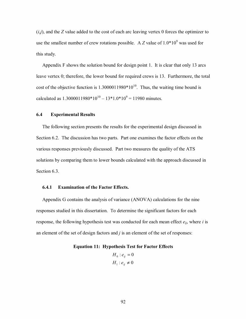
92

(i,j), and the Z value added to the cost of each arc leaving vertex 0 forces the optimizer to

use the smallest number of crew rotations possible. A Z value of 1.0*109 was used for

this study.

Appendix F shows the solution bound for design point 1. It is clear that only 13 arcs

leave vertex 0; therefore, the lower bound for required crews is 13. Furthermore, the total

cost of the objective function is 1.3000011980*1010. Thus, the waiting time bound is

calculated as 1.3000011980*1010 – 13*1.0*109 = 11980 minutes.

6.4 Experimental Results

The following section presents the results for the experimental design discussed in

Section 6.2. The discussion has two parts. Part one examines the factor effects on the

various responses previously discussed. Part two measures the quality of the ATS

solutions by comparing them to lower bounds calculated with the approach discussed in

Section 6.3.

6.4.1 Examination of the Factor Effects.

Appendix G contains the analysis of variance (ANOVA) calculations for the nine

responses studied in this dissertation. To determine the significant factors for each

response, the following hypothesis test was conducted for each mean effect eij, where i is

an element of the set of design factors and j is an element of the set of responses:

Equation 11: Hypothesis Test for Factor Effects

0:

0:

1

0

≠

=

ij

ij

eH

eH

93

The p-value of each eij was used as the test statistic for the hypothesis test. It is a

standard test statistic and is defined as follows:

The p-value is the smallest level of significance, α, at which H0 would be rejected when a specified test procedure is used on a given data set. Once the p-value has

been determined, the conclusion at any particular level α results from comparing the p-value to α:

1) p-value ≤ α ⇒ reject H0 at level α. 2) p-value > α ⇒ do not reject H0 at level α. (Devore, 1991:315)

Analysis of variance was used on each data set, hence the p-value relates to a standard

F-test conducted for each factor/response combination. An α value of 0.05 was used for

all hypothesis tests performed in this research.

Table 4 shows the mean effects of each design factor with respect to the number of

crews and total waiting time (WT) in the ATS’s best feasible (F) and best near feasible

(NF) solutions. Table values of X indicate that H0 above was not rejected, hence the

factor was found to be insignificant for that particular response.

It is clear that, for the TCSP’s two objectives, the characteristics of the flight schedule

dominate the solution. Especially significant are the number of rotations generated each

day and the length of the schedule. This is to be expected--longer schedules and higher

operational tempos require more crews and increase the amount of wait time for those

crews.

As the maximum distance in the base network and refueling times increased, so did

the number of crews required and the waiting time of the crews. This appears to be a

function of crew reusability. The increased distances and refueling times create longer

94

refueling flights; hence the crews are busy for longer periods of the duty day and cannot

be assigned to other flights.

The rotation departure time also has a notable effect on the two objectives. When the

rotation departure time is clustered, it significantly tightens the schedule. Crews cannot

be reused because there are a large number of flights taking off in the same time period.

Since rotation departures are clustered, the waiting time increases because once a crew

completes their duty day, operations do not restart until 0000 hours the next day. When

departures are uniform throughout the day, the crews are reused more quickly and their

waiting time on the ground is reduced.

PCF is insignificant for all the responses. This supports the intuition that crew flying

histories will likely not affect the two objectives until the flying schedules examined are

larger, i.e. 30+ day schedules.

The type of tabu tenure used and the value for the ISGS counter do not significantly

affect the ATS solutions, but the higher value for the CP counter increases the total

waiting time in feasible and near feasible ATS solutions. This is to be expected. When

the search trajectory becomes severely entrenched in areas of poor infeasibility, it is

difficult to escape and the ATS must use the TCRSIN for a larger number of iterations.

This targeted neighborhood directs the trajectory toward feasibility, but in the process, it

appears to hinder the model’s ability to find the better waiting time solutions. The

obvious solution is to use the low CP value and not allow the trajectory to delve so

deeply into areas of poor infeasibility.

Finally, the intensification scheme performs as well as the ATS with vocabulary

building for all responses but the total waiting time in near feasible solutions. The main

95

contribution of the vocabulary building scheme is its ability to solve the TCSP much

more quickly than the ATS with intensification, as discussed below.

Table 4: Factor Effects for the TCSP objectives Factor ATS F Crews ATS NF Crews ATS F WT ATS NF WT

Average Value 40.151 37.557 165491 156037 Rot/day 21.302 19.990 81514 78895

NumBases 5.781 5.302 27520 25023 TBF X X X X TBR X X X X

NumDIS 19.177 18.740 302248 286065 MDIBN 1.823 2.198 X X

RS 7.802 7.219 31964 28913 RT 10.177 10.656 29776 31765

RDT 12.073 11.656 26500 26197 PCF X X X X

MWBF 3.990 4.865 19046 23645 Tenure X X X X ISGS X X X X CP X X 18608 17086

Intensification/VB X X X -15546 With a discussion of the two TCSP objectives complete, the remainder of this section

examines the affect of the design factors on various ATS performance measures. Table 5

displays the mean effects for each of the factors.

As seen for the TCSP objectives, many of the ten flight schedule factors significantly

affect tabu search performance measures such as total solution time and the number of

conjugacy classes visited. When the number of daily rotations generated and number of

days in the schedule increase, the size of the resulting flight schedules increases. Table 5

shows that as the size of these flight schedules increase, there is more opportunity to

improve the initial solution and the number of iterations and the total solution time

increases.

96

As the flight schedule sizes increase, the size of the solution space, Sn, increases. The

ATS appears to respond to an increased solution space size by increasing the tabu tenure.

This limits cycling and forces the search to different parts of the solution space. This

increase in diversification corresponds to visiting a larger number of conjugacy classes.

Notice that clustering rotation departure times decreases the values of all tabu search

responses but the average neighborhood size. This supports the intuition that flight

schedules with clustered departures are much tighter, meaning there is much less

opportunity to improve the initial solution. In effect, the clustered departure times prune

a significant portion of Sn from consideration. This solution space reduction is seen as a

large decrease in the number of conjugacy classes visited. Since the ATS does not

diversify often, it terminates sooner, decreasing the number of iterations and total

solution time. The number of iterations completed bounds the tabu tenure, i.e., if 10

iterations have been completed, the tabu tenure is effectively 10 at the high level.

Therefore, decreasing the number of iterations decreases the average tabu tenure.

The tabu search factors ISGS and CP significantly affect the ATS performance. As

ISGS increases, the number of iterations and total solution time increases, as does the

average tabu tenure. This larger average tabu tenure indicates that the ATS tends to cycle

when the solution does not improve for long periods of time. Note that this increase in

computational cost comes with no improvement in the two TCSP objectives.

When the search is permitted to stay in areas of poor infeasibility too long, the number

of conjugacy classes visited severely decreases. The search becomes trapped in a smaller

region of the solution space. This seems to explain the degradation of the total waiting

time in feasible and near feasible ATS solutions at the high CP level.

97

Vocabulary building clearly improves the performance of the adaptive tabu search

developed in this research. It is the most significant factor with respect to the number of

iterations completed, reducing termination by 8459 iterations. This is over twice the

magnitude of the next most significant mean effect. While CPLEX took a significant

amount of time to solve the vocabulary building SPPs, the strategy worked so well that it

overcame this limitation and still reduced the TST by over 28 minutes. This is very

significant considering the average TST is approximately 36 minutes. Where the

intensification scheme forces the ATS to traverse a large number of conjugacy classes to

find good solutions, vocabulary building avoids these classes and moves rapidly to

excellent areas of the solution space.

Table 5: Factor Effects for Number of Iterations, Total Solution Time, Number of Conjucacy Classes Visited, Ave Neighborhood Size, and Ave Tabu Tenure

Factor Iterations TST Num CC Visited Ave NS Ave Tabu Tenure Average Value 6089 2149.1 895.6 1822.3 2541

Rot/day 2207 2832.8 X 1887.5 1031 NumBases X X X -439.8 X

TBF X X X X X TBR X X X X X

NumDIS 3845 4103.8 1742.9 2643.3 1339 MDIBN X X X 117.3 X

RS X X 395.9 X X RT X X -470.3 X X

RDT -1980 -1299.1 -705.5 X -760 PCF X X X X X

MWBF X X X X X Tenure X X X X 737 ISGS 3721 1039.9 X X 1474 CP X X -544.1 X X

Intensification/VB -8459 -1687.5 -642.2 X -4116

As discussed in Section 3.3, Hooker suggests that once controlled experiments are run

over a variety of parameter settings and the effects of the parameter settings examined,

98

the choice of levels should be clear (1995:40). This appears true for the ATS developed

in this research.

Clearly, vocabulary building should be used within the ATS framework. At the high

level, ISGS increases computational time while providing no improvement in finding

good feasible or near feasible solutions. Thus, ISGS should be set to the low level of 250.

While the values for CP do not affect computational time, they clearly hinder the

performance of the ATS by terminating at solutions with increased waiting time.

Therefore, CP should also be set at the low level. Finally, either tabu tenure scheme

appears robust and could be implemented.

6.4.2 Comparing the ATS Solutions to Lower Bounds.

To measure the quality of the ATS solutions, the following section examines the

number of assigned crews and total waiting time for the initial and best feasible ATS

solutions with respect to the lower bounding scheme developed in Section 6.3. The

starting solutions are examined for two reasons:

1) To show that the initial heuristic finds good solutions.

2) To examine the amount of improvement gained by implementing the ATS.

The performance measure used is the percentage distance from the respective bound:

Equation 12: Calculating % Distance from the Lower Bound

}. , {∈}, , {∈ where

,

) (= %

TimeWaitingTotalCrewsofNumberjSolutionStartingSolutionATSi

valueboundvalueboundvalueactual

distj

jijij

99

Appendix E contains the data on the respective % distance calculations. In addition to

reducing the % distance as compared to the starting solution, the ATS solutions are much

less variable. Table 6 below summarizes the data on the average and standard deviation

for each respective % distance.

The heuristic used to create starting solutions for the ATS appears to create good

initial solutions. It provides solutions, on average, within 7.71 of the crew bound and

within 13.51 percent of the waiting time bound. The ATS does an excellent job of

improving these solutions. With respective percentage distances of 3.78 and 5.03, the

ATS reduces the distance from the crew bound by more than half and reduces the

distance from the waiting time bound by nearly 63%. In addition to reducing the mean %

distance, it is clear that the ATS solutions are much less variable as well, nearly halving

the standard deviation in each TCSP objective.

Table 6: Ave and Standard Deviation for % Distance with Respect to the Lower Bounds

ATS Num Crews

ATS Wait Time

Starting Num Crews

Starting Wait Time

Ave % dist 3.78 5.03 7.71 13.51 SD % dist 5.82 7.27 10.58 14.35

The table in Appendix E shows many instances where the ATS solution matches the

lower bounds on number of crews and total waiting time. Since all ATS solutions shown

are feasible, and the lower bounds show that no smaller crew or waiting time solution

exists, these ATS solutions are optimal. Indeed, the ATS can be shown to find the

optimal solution for nearly 40% of the problems solved in the designed experiment.

100

The lower bounding scheme does not guarantee that the bound found is a feasible

solution. The ATS may be finding optimal solutions although its solution does not match

the lower bounds. Therefore, the 40% optimality described above is a lower bound on

the percentage of problems for which the ATS finds the optimal solution. The next

section identifies design points where the ATS solution does not match the lower bound

but is the optimal solution.

6.4.3 Comparing ATS Solutions to Known Optimal Solutions.

The following section examines a number of smaller TCSPs. These problems allow

enumeration of all feasible crew rotations. For each problem, the known optimal solution

is found by solving two SPPs, with each feasible crew rotation a column of the SPP. The

first SPP minimizes the number of crews in the solution. The number of crews in the

optimal solution to the first SPP is added as a constraint to the second SPP, which

minimizes total waiting time.

Forty-four of the problems in the experimental design are small enough to find the

optimal solution. Appendix H summarizes each design problem’s % distance from the

optimal solution, and indicates whether the ATS solution is optimal or sub-optimal. This

is calculated as in Equation 12, but the bound value is replaced by the optimal value. The

results show that the ATS finds the optimal solution to 40 of the 44 problems. The 40

optimal ATS solutions are not shown to be optimal by the lower bounds. Therefore,

adding them to the previous list of known optimal solutions, the ATS finds the optimal

solution for nearly 60% of all problems in the experimental design.

101

Of course, the ATS is a metaheuristic and is not guaranteed to find the optimal

solution. Table 7 below summarizes the results for the four problems out of 44 where the

ATS solution is not optimal. The results show the ATS still found excellent solutions.

The average % distance from the optimal number of crews and optimal waiting time is

only 0.86% and 1.00%, respectively.

Table 7: Summary of Four Sub-optimal ATS Solutions in the Experimental Design Design Point Optimal # Crews Optimal Wait Time ATS # Crews ATS Wait Time

101 26 21321 26 21352 102 25 25094 25 25342 121 30 23102 30 23232 134 29 27503 30 28138

While the ATS performed well for the problems found in the designed experiment, a

natural follow-on question is, “How will the ATS perform on a problem found outside

the design space or a problem of significantly larger size?” The next section addresses

this issue.

6.4.4 Solving a Very Large TCSP.

The following section discusses the ATS performance on a very large TCSP. The

problem simulates a 30-day deployment scenario. The deployment surges in the first

week, generating 40 rotations each day. The tempo slows for the remainder of the

schedule, generating only 15 rotations per day for the last three weeks. Table 8 displays a

complete listing of the problem characteristics. The resulting schedule contains 1269

flights. This schedule is three times the size of the largest schedule in the experimental

102

design, and over 11.5 times the size of the schedule produced by Wiley’s largest

deployment scenario (Wiley, 2001).

Table 8: Characteristics of a Large Deployment Operation

Factor Value Rot/day 40 1st week, 15 weeks 2-4

NumBases 8 TBF 60 min TBR 360 min

NumDIS 30 MDIBN 485 min

RS 25% 1, 50% 2, 25% 3 RT T(180,240,300) min

RDT Uniform PCF 0.50

MWBF 60/240 min

An ATS with vocabulary building scheme is used to solve the problem. ISGS is set to

250, CP to 25, PCF to 0.50, and the MWFB to 60/240 minutes. The ATS produces a

feasible initial solution with 118 crews and 3334175 minutes of total waiting time.

Figure 14 shows the progress of the ATS with respect to minimizing the number of crews

in a feasible solution. Figure 15 shows the progress with respect to minimizing total

waiting time. The square boxes on the graphs represent points of vocabulary building.

At the beginning of the search, little progress is made in terms of the number of crews in

the solution, but total waiting time of those crews is being reduced significantly.

By iteration 365, about 27 minutes after starting the solution process, a feasible

solution with 3087760 minutes of waiting time is found. This is a 7.4% reduction in

waiting time, a savings of 246415 minutes or about 171 days.

103

114

115

116

117

118

119

0

312

624

936

1248

1560

1872

2184

2496

2808

3120

3432

3744

4056

4368

4680

4992

5304

Iterations

Num

ber o

f Fea

sibl

e C

rew

s

Figure 14: Finding the Smallest Feasible Number of Crews in a Large TCSP.

25000002600000270000028000002900000300000031000003200000330000034000003500000

0

358

716

1074

1432

1790

2148

2506

2864

3222

3580

3938

4296

4654

5012

5370

Iterations

Tota

l Wai

t Tim

e

Figure 15: Finding the Smallest Total Wait Time in a Large TCSP.

At this point, the ATS seems to stall and no crew or waiting time improvements are

made for a long period of time. But the ATS does not terminate at any time during this

stretch because the vocabulary building continues to improve the best near feasible

104

solutions. At iteration 2421, about 3.5 hours into the solution process, vocabulary

building sends the trajectory of the search into a significantly better portion of the

solution space. A 17 crew feasible solution is found in the next neighborhood evaluation.

The total waiting time of this solution is 2754589. At this point in the search, total

waiting time has been reduced by 17.38%, a savings of 579586 minutes or about 402

days.

The ATS continues to improve the solution until at iteration 5263, the best solution is

found by solving a SPP. The best solution has 15 crews and 2667124 minutes of total

waiting time. This is a savings of 3 crews and a reduction in total waiting time of 20%, a

savings of 667051 minutes or about 463 days! The ATS terminates 255 iterations after

finding the best solution. The total solution time is just over 8 hours.

In conclusion, this chapter met all its objectives. It examined various factors of the

TCSP and ATS to determine their effects on solution quality and ATS performance. It

clearly showed the effectiveness of embedding SPP-based vocabulary building within the

ATS. It then provided a lower bounding scheme to measure the quality of ATS solutions.

It compared ATS solutions to known optimal solutions, supporting the excellence of the

approach. Finally, it showed the effectiveness of the ATS on a large-scale deployment

schedule.

105

VII Concluding Remarks This chapter details the major contributions of this research and discusses future

avenues of research for the TCSP and the methodologies developed.

7.1 Major Contributions

This section discusses the many contributions produced by this research. It begins by

discussing the contributions to the general operations research community and concludes

by discussing the various USAF contributions.

7.1.1 Operations Research Contributions.

This research presents the first metaheuristic approach to the complete air crew

scheduling problem. It simultaneously pairs flights and rosters them to individual crews.

Although the excellence of the tabu search approach has been shown with application to

tanker crew scheduling, FAA and airline rules and objectives could be substituted for the

Air Force regulations and objectives to obtain a tabu search suitable for their needs.

Furthermore, the methodology can be extended to any scheduling problem that requires a

time-dependent assignment of one set of resources to another set of resources. The

underlying theoretic tabu search mechanisms remain identical.

This research presents the first use of dynamic, integrated, set-partitioning based,

vocabulary building within a metaheuristic search. The effectiveness of the integrated

vocabulary builder within the adaptive tabu search has clearly been shown. This

methodology can be extended to any problem that has an underlying set partioning or set

covering solution structure.

106

This research defined and created the first general flight schedule generator. This new

generator will allow future researchers to create benchmark data sets when studying their

air crew scheduling problems. The generator allowed the creation of the benchmark data

set used to conduct a statistical analysis of our ATS, an area routinely ignored by other

researchers. This analysis included the development of integer programming-based

lower bounds that helped measure the quality of the ATS process.

This research demonstrates the effective use of group theory as a tabu search

foundation. It shows group theory provides an excellent solution structure for

combinatorial problems such as the TCSP. It develops effective solution and conjugacy

class hash functions. It demonstrates the effectiveness of template-based inserts and

conjugation-based swaps. Finally, it provides a new measure of tabu search

diversification by using conjugacy class frequency information.

7.1.2 USAF Contributions.

The methodology developed in this research provides a rigorous analytic foundation

for determining the number of crews required to fly aircraft schedules, as opposed to the

back-of-the-envelope calculations so often used. Air Force analysts can develop a variety

of scenarios and determine crew ratios using the ATS or ATS/SPP hybrid.

The ATS provides a means for air mobility analysts to conduct deeper analyses. In

addition to answering questions on the number of crews required, they can also study

problems such as:

1) How does operations during peace affect our crew operations during war?

2) How should crews be distributed within a base network to most effectively utilize them?

107

Besides peacetime planning, the tool can be used during operations. Given an air

refueling schedule, the ATS provides a good crew schedule. Within an air operations

center, crew schedulers could use the tool to answer “what if” questions like: Is the air

refueling schedule produced feasible given the flying history of our crews? Coupled with

an air refueling scheduler, it should allow a more intense flying schedule or detect severe

risks in the given schedule. Finally, the tabu search is easily extended to other Air Force

problems, such as scheduling crews for the airlift community.

7.2 Avenues for Future Research

While completing this research, many future avenues of research appeared. This

section provides a description of these avenues.

A novice programmer created the JavaTM code for this research. While it finds

excellent solutions in a reasonable amount of time, there likely are inefficiencies to be

found in the code. An in-depth analysis by an expert programmer could uncover such

and reduce solution times.

During vocabulary building, as the set partitioning problems become large, the time to

solve the SPP portion of the problem begins to overwhelm the search. The ten-minute

solution time limit is routinely reached by CPLEX, and heuristic solutions are ultimately

produced. Research should be conducted to find a faster SPP solver within the hybrid

scheme. One alternative may be to embed a SPP metaheuristic solver within the hybrid.

A second would be to examine a previously developed large-scale SPP solver and

develop JavaTM wrappers or a JavaTM version of it.

108

The ATS uses a relatively simple insert and swap neighborhood to conduct its search.

This neighborhood performed excellently, but follow-on research could examine the

utility of implementing more complicated neighborhoods. Future research could also

examine other adaptive tabu search schemes, or extend the adaptive scheme to the

reactive tabu search developed by Battiti and Tecchiolli (1994). It would be interesting

to compare the reactive tabu search to the ATS with vocabulary building, and to study

whether or not vocabulary building increases the effectiveness of the reactive tabu search.

This research directly follows Wiley’s Aerial Refueling dissertation (2001). Wiley’s

tabu search provides the tanker refueling input for our crew scheduler. The two tools

produced by these efforts need to be combined. One solution is a sequential approach

where the aerial fleet refueling problem is solved, feeds the resulting schedule to the crew

scheduler, and the TCSP is solved. An alternative approach is to solve the aerial fleet

refueling problem and TCSP simultaneously. The objectives and constraints of each

problem could be combined to form a larger problem suitable for metaheuristic search.

The combined problem may yield solutions unattainable by the sequential approach.

This research focused on solving the TCSP. The ATS approach developed can clearly

be applied to other USAF flying communities. Demonstration of this would be

beneficial, along with further extension to the airlines’ crew scheduling problem.

Extensions can be made to the flight schedule generator. For example, to generate

random variates from different probability distributions, users have to rely on outside

JavaTM objects. Embedding such a probability class within the generator itself would

alleviate the need for this.

109

7.3 Conclusions

This research contributes significantly to the operations research community. It

provides the first metaheuristic approach for solving the complete air crew scheduling

problem. This methodology can be extended to other crew scheduling problems. It

provides the first dynamic, integrated, set-partitioning based vocabulary building scheme.

This vocabulary building methodology may be exploited by other problems that have

underlying set partitioning or set covering solution structures. It provides a general,

reusable flight schedule generator. The research highlights the insights to be gained

when conducting statistical analysis on metaheuristics. Finally, it opens many avenues

for future research. Future researchers should be able to extend the methodologies

provided and build better approaches to other combinatorial problems.

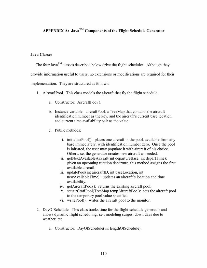
110

APPENDIX A: JavaTM Components of the Flight Schedule Generator

Java Classes

The four JavaTM classes described below drive the flight scheduler. Although they

provide information useful to users, no extensions or modifications are required for their

implementation. They are structured as follows:

1. AircraftPool. This class models the aircraft that fly the flight schedule.

a. Constructor: AircraftPool(). b. Instance variable: aircraftPool, a TreeMap that contains the aircraft

identification number as the key, and the aircraft’s current base location and current time availability pair as the value.

c. Public methods:

i. initializePool(): places one aircraft in the pool, available from any

base immediately, with identification number zero. Once the pool is initiated, the user may populate it with aircraft of his choice. Otherwise, the generator creates new aircraft as needed.

ii. getNextAvailableAircraft(int departureBase, int departTime): given an upcoming rotation departure, this method assigns the first available aircraft.

iii. updatePool(int aircraftID, int baseLocation, int newAvailableTime): updates an aircraft’s location and time availability.

iv. getAircraftPool(): returns the existing aircraft pool; v. setAirCraftPool(TreeMap tempAircraftPool): sets the aircraft pool

to the temporary pool value specified. vi. writePool(): writes the aircraft pool to the monitor.

2. DayOfSchedule. This class tracks time for the flight schedule generator and

allows dynamic flight scheduling, i.e., modeling surges, down days due to weather, etc.

a. Constructor: DayOfSchedule(int lengthOfSchedule).

111

b. Instance variables: i. dayOfSchedule: an integer that represents the current day of the

schedule. ii. lengthOfSchedule: an integer that represents how many days the

aircraft should fly.

c. Public methods:

i. getDayOfSchedule(): allows access to the current day by any class.

ii. getLengthOfSchedule(): allows access to the length of schedule. iii. setDayOfSchedule(int newDay): sets the flight schedule day. iv. setLengthOfSchedule(int length): sets the length of the aircraft

schedule.

3. Schedule. This class models the flight schedule itself, the fundamental input to the crew scheduling process.

a. Constructor: Schedule(). b. Instance variable: flightSchedule, a JavaTM ArrayList representing the

aircraft flight schedule. c. Public methods:

i. addFlight(int[] flight): this method adds a flight to the schedule.

ii. getFlightSchedule(): returns the flight schedule at any point in time.

iii. setFlightSchedule(ArrayList tempFlightSchedule): sets the flight schedule to the arraylist passed as a parameter.

iv. printToScreen(): prints the flight schedule to the monitor. v. clearFlightSchedule(): clears the flight schedule, primarily used

when randomly generating multiple flight schedules.

4. FlightScheduler. This class provides the engine for the flight schedule generator. It contains the algorithm used to generate a schedule, and writes each iteration to output files.

a. Constructor: FlightScheduler (AircraftPool aircraftPool, DayOfSchedule

timeKeeper, Rotation rotation, Flight flight, BaseNetwork network, Schedule flightSchedule, int scheduledDays, int numberOfIterations, String outputDirectory).

112

b. Instance variables:

i. aircraftPool: an instantiation of the aircraft pool.

ii. timekeeper: an instantiation of the DayOfSchedule object. iii. flightSchedule: an instantiation of the flight schedule. iv. scheduledDays: an integer representing the length of the flight

schedule. v. numberOfIterations: an integer representing the number of flight

schedules generated. vi. outputDirectory: a string declaring where the output files should

be placed.

The following represent instantiations of objects using the interfaces described below.

vii. rotation: an instantiated Rotation object viii. network: an instantiated base network.

ix. flight: an instantiated Flight object.

c. Public methods: generateFlightSchedule(): this method generates the flight schedules using the generator algorithm described in Chapter V.

Java Interfaces

The three JavaTM interfaces detailed below describe the characteristics of the flight

scheduler. They contain no constructors or instance variables. Instead, they simply

define empty, abstract methods that the user must override when implementing an

interface. The interfaces allow the generalization of the generator. By overriding the

abstract methods, users create flight schedules representing their own scenario. The

characteristics may be as simple or complicated as the user desires.

1. Rotation. This interface models an aircraft rotation. The following abstract methods must be overridden to implement the Rotation interface:

a. getRotationLength(): returns an integer representing the number of flights

contained in each rotation. b. getRotationHomeBase(): returns an integer representing the base of

departure of the rotation. c. getRotationDepartureTime(): returns an integer representing the time at

which the rotation departs.

113

d. getRotationReturnBase(): returns an integer representing the base on which the rotation terminates.

e. getNumberOfRotations(): returns an integer representing the number of

rotations to be initiated each day. f. getAircraftDownTime(): returns an integer representing the amount of

time an aircraft must rest before it begins another rotation.

2. Flight. This interface models an aircraft flight. A flight is simply a departure and arrival of an aircraft, with some quantity of flying time defined between the events. The following methods must be overridden to implement the interface:

a. getFlightTimeExtension(): This method returns an integer representing

deviations added to the flight time between bases. b. getArrivalBase(): returns an integer representing the arrival base of the

flight. c. getAircraftTurnTimes(): returns an integer representing the amount of

time it takes to turn an aircraft after a flight. For example, in a civilian airline schedule time is needed to unload the passengers, clean the cabin, and then load the new set of passengers.

3. BaseNetwork. This interface represents the network in which the aircraft operate.

It contains one method that must be overridden, generateBaseNetwork(). This method returns a two-dimensional integer array containing the flying times between the bases.

114

APPENDIX B: Using the Flight Schedule Generator

While it is important to understand the inner workings of the flight schedule generator,

an issue likely more important to the typical user is, “How do we implement the flight

schedule generator for our application?” The following section discusses implementation

issues, step-by-step, by way of a small example.

Suppose a flight schedule with the following characteristics needs to be created:

1. All flights depart and arrive at a single base. 2. The schedule length is two days. 3. Five rotations of length two are initiated each day. 4. The rotations depart uniformly throughout the day. 5. Time between flights in a rotation is sixty minutes. 6. Down time between rotations is 360 minutes. 7. Each flight generated from the base is 240 minutes long.

This example is obviously simplistic, but it allows demonstration of the basic steps

required to use the generator.

The first step for implementation is creating the class files that implement the

BaseNetwork, Rotation, and Flight interfaces. The following is the code required to

implement each and serves as a framework for more complicated classes.

Base Network Implementation:

import combs.flightscheduler.*; public class ExampleBaseNetwork implements BaseNetwork{ public ExampleBaseNetwork(){ } public int[][] generateBaseNetwork(){ int[][] baseNetwork = {{0}}; return baseNetwork; }

115

} Notice the first statement in the ExampleBaseNetwork class, import

combs.flightscheduler.*. The flight schedule generator is packaged in a Java Archive

(JAR) file called flightscheduler.jar. Each of the three user-defined classes described

above must have this import statement to use the generator. The base network class

simply creates a base network of size one with zero inter-base flying time.

Rotation Implementation:

import combs.flightscheduler.*; import drasys.or.prob.*; public class ExampleRotation implements Rotation{ //Instance variables private DayOfSchedule exampleDayOfSchedule; private DiscreteUniformDistribution rotationDepartTime; //Create a constructor public ExampleRotation(DayOfSchedule dayOfSchedule){ rotationDepartTime = new DiscreteUniformDistribution(0,1,1440,1); this.exampleDayOfSchedule = dayOfSchedule; } //Implement the various rotation methods public int getRotationLength(){ return 2; } public int getRotationHomeBase(){ return 0; } public int getRotationDepartureTime(){ int day = exampleDayOfSchedule.getDayOfSchedule(); int departureTime = (1400*(day-1) + rotationDepartTime.getRandomInteger()); return departureTime; } public int getRotationReturnBase(){ return 0; }

116

public int getNumberOfRotations(){ return 5; } public int getAircraftDownTime(){ return 360; } }

The Rotation class demonstrates another advantage of building the generator with an

object-oriented language such as JavaTM. Users can build their own schedules using

previously built classes, such as the probability classes found in OR-Objects on

www.opsresearch.com (2002). The ExampleRotation class uses the

DiscreteUniformDistribution class to spread departures uniformly throughout each

scheduled day.

Flight Implementation:

import combs.flightscheduler.*; public class ExampleFlight implements Flight{ //Constructor public ExampleFlight(){ } //Implement the various flight methods public int getFlightTimeExtension(){ return 240; } public int getArrivalBase(){ return 0; } public int getAircraftTurnTimes(){ return 60; } }

Once the implementation classes are built, a main class has to be built to instantiate all

objects and run the flight schedule generator. The main class for this example follows.

117

Main Class:

import combs.flightscheduler.*; public class ExampleScheduler { public static void main(String args[]) { //Set the # of days in the schedule int scheduleLength = 2; //Set the # of iterations int numberIterations = 1; //Instantiate an aircraft pool object AircraftPool aircraftPool = new AircraftPool(); //Instantiate a day of schedule object DayOfSchedule exampleDayOfSchedule = new DayOfSchedule(scheduleLength); //Instantiate a flight schedule object Schedule exampleFlightSchedule = new Schedule(); //Instantiate a flight object ExampleFlight exampleFlight = new ExampleFlight(); //Instantiate a rotation object ExampleRotation exampleRotation = new ExampleRotation(exampleDayOfSchedule); //Instantiate a base network object ExampleBaseNetwork exampleBaseNetwork = new ExampleBaseNetwork(); //Instantiate a flight scheduler object FlightScheduler exampleFlightScheduler = new FlightScheduler(aircraftPool, exampleDayOfSchedule, exampleRotation, exampleFlight, exampleBaseNetwork, exampleFlightSchedule, scheduleLength, numberIterations,

"/ExampleScheduler/"); exampleFlightScheduler.generateFlightSchedule(); } }

The ExampleScheduler class follows a sequence that must be done for any

application:

1. Set the schedule length and number of iterations desired. 2. Instantiate all flight schedule classes. Before running the scheduler, ensure

that the output directory specified in the FlightScheduler object already exists in the specified location.

3. Call the generateFlightSchedule() method to generate the flight schedule(s).

118

Once these four classes are created, the user is ready to generate flight schedules. We

recommend placing all jar and class files in the same directory when running the

generator. A good location is a user-defined directory within the bin directory of the

JavaTM software. Once this is done, the code must be compiled and run. The commands

for this example are:

1. javac -classpath .;flightscheduler.jar;or124.jar.zip *.java 2. java -classpath .;flightschedule.jar;or124.jar.zip ExampleScheduler

The example schedule produced captures the desired characteristics.

Table 9: Example Flight Schedule

Aircraft ID Departure Base Departure Time Flight Time Arrival Base Arrival Time 0 0 229 240 0 469 0 0 529 240 0 769 1 0 701 240 0 941 1 0 1001 240 0 1241 2 0 776 240 0 1016 2 0 1076 240 0 1316 3 0 1109 240 0 1349 3 0 1409 240 0 1649 0 0 1393 240 0 1633 0 0 1693 240 0 1933 1 0 1796 240 0 2036 1 0 2096 240 0 2336 2 0 1823 240 0 2063 2 0 2123 240 0 2363 3 0 2093 240 0 2333 3 0 2393 240 0 2633 0 0 2298 240 0 2538 0 0 2598 240 0 2838 1 0 2787 240 0 3027 1 0 3087 240 0 3327

119

APPENDIX C: Resolution IV Experimental Design

DP = Design Point A = Rot/day B = NumBases C = TBF D = TBR E = NumDIS F = PCF G = ISGS H = CP I = MDIBN J = RS K = RT L = RDT M = MWBF N = tenure O = Intensify/VB

DP A B C D E F G H I J K L M N O 1 -1 -1 -1 -1 -1 -1 -1 -1 -1 1 -1 -1 -1 1 1 2 -1 -1 -1 -1 -1 -1 -1 -1 -1 1 -1 -1 -1 1 1 3 -1 -1 -1 -1 -1 -1 -1 -1 -1 1 -1 -1 -1 1 1 4 -1 -1 -1 -1 -1 1 1 1 1 1 1 1 1 1 -1 5 -1 -1 -1 -1 -1 1 1 1 1 1 1 1 1 1 -1 6 -1 -1 -1 -1 -1 1 1 1 1 1 1 1 1 1 -1 7 -1 -1 -1 -1 1 -1 1 1 1 -1 -1 -1 -1 1 -1 8 -1 -1 -1 -1 1 -1 1 1 1 -1 -1 -1 -1 1 -1 9 -1 -1 -1 -1 1 -1 1 1 1 -1 -1 -1 -1 1 -1

10 -1 -1 -1 -1 1 1 -1 -1 -1 -1 1 1 1 1 1 11 -1 -1 -1 -1 1 1 -1 -1 -1 -1 1 1 1 1 1 12 -1 -1 -1 -1 1 1 -1 -1 -1 -1 1 1 1 1 1 13 -1 -1 -1 1 -1 -1 1 -1 -1 -1 1 -1 -1 -1 -1 14 -1 -1 -1 1 -1 -1 1 -1 -1 -1 1 -1 -1 -1 -1 15 -1 -1 -1 1 -1 -1 1 -1 -1 -1 1 -1 -1 -1 -1 16 -1 -1 -1 1 -1 1 -1 1 1 -1 -1 1 1 -1 1 17 -1 -1 -1 1 -1 1 -1 1 1 -1 -1 1 1 -1 1 18 -1 -1 -1 1 -1 1 -1 1 1 -1 -1 1 1 -1 1 19 -1 -1 -1 1 1 -1 -1 1 1 1 1 -1 -1 -1 1 20 -1 -1 -1 1 1 -1 -1 1 1 1 1 -1 -1 -1 1 21 -1 -1 -1 1 1 -1 -1 1 1 1 1 -1 -1 -1 1 22 -1 -1 -1 1 1 1 1 -1 -1 1 -1 1 1 -1 -1

120

23 -1 -1 -1 1 1 1 1 -1 -1 1 -1 1 1 -1 -1 24 -1 -1 -1 1 1 1 1 -1 -1 1 -1 1 1 -1 -1 25 -1 -1 1 -1 -1 -1 -1 1 -1 -1 -1 1 -1 -1 -1 26 -1 -1 1 -1 -1 -1 -1 1 -1 -1 -1 1 -1 -1 -1 27 -1 -1 1 -1 -1 -1 -1 1 -1 -1 -1 1 -1 -1 -1 28 -1 -1 1 -1 -1 1 1 -1 1 -1 1 -1 1 -1 1 29 -1 -1 1 -1 -1 1 1 -1 1 -1 1 -1 1 -1 1 30 -1 -1 1 -1 -1 1 1 -1 1 -1 1 -1 1 -1 1 31 -1 -1 1 -1 1 -1 1 -1 1 1 -1 1 -1 -1 1 32 -1 -1 1 -1 1 -1 1 -1 1 1 -1 1 -1 -1 1 33 -1 -1 1 -1 1 -1 1 -1 1 1 -1 1 -1 -1 1 34 -1 -1 1 -1 1 1 -1 1 -1 1 1 -1 1 -1 -1 35 -1 -1 1 -1 1 1 -1 1 -1 1 1 -1 1 -1 -1 36 -1 -1 1 -1 1 1 -1 1 -1 1 1 -1 1 -1 -1 37 -1 -1 1 1 -1 -1 1 1 -1 1 1 1 -1 1 1 38 -1 -1 1 1 -1 -1 1 1 -1 1 1 1 -1 1 1 39 -1 -1 1 1 -1 -1 1 1 -1 1 1 1 -1 1 1 40 -1 -1 1 1 -1 1 -1 -1 1 1 -1 -1 1 1 -1 41 -1 -1 1 1 -1 1 -1 -1 1 1 -1 -1 1 1 -1 42 -1 -1 1 1 -1 1 -1 -1 1 1 -1 -1 1 1 -1 43 -1 -1 1 1 1 -1 -1 -1 1 -1 1 1 -1 1 -1 44 -1 -1 1 1 1 -1 -1 -1 1 -1 1 1 -1 1 -1 45 -1 -1 1 1 1 -1 -1 -1 1 -1 1 1 -1 1 -1 46 -1 -1 1 1 1 1 1 1 -1 -1 -1 -1 1 1 1 47 -1 -1 1 1 1 1 1 1 -1 -1 -1 -1 1 1 1 48 -1 -1 1 1 1 1 1 1 -1 -1 -1 -1 1 1 1 49 -1 1 -1 -1 -1 -1 -1 -1 1 -1 -1 -1 1 -1 -1 50 -1 1 -1 -1 -1 -1 -1 -1 1 -1 -1 -1 1 -1 -1 51 -1 1 -1 -1 -1 -1 -1 -1 1 -1 -1 -1 1 -1 -1 52 -1 1 -1 -1 -1 1 1 1 -1 -1 1 1 -1 -1 1 53 -1 1 -1 -1 -1 1 1 1 -1 -1 1 1 -1 -1 1 54 -1 1 -1 -1 -1 1 1 1 -1 -1 1 1 -1 -1 1 55 -1 1 -1 -1 1 -1 1 1 -1 1 -1 -1 1 -1 1 56 -1 1 -1 -1 1 -1 1 1 -1 1 -1 -1 1 -1 1 57 -1 1 -1 -1 1 -1 1 1 -1 1 -1 -1 1 -1 1 58 -1 1 -1 -1 1 1 -1 -1 1 1 1 1 -1 -1 -1 59 -1 1 -1 -1 1 1 -1 -1 1 1 1 1 -1 -1 -1 60 -1 1 -1 -1 1 1 -1 -1 1 1 1 1 -1 -1 -1 61 -1 1 -1 1 -1 -1 1 -1 1 1 1 -1 1 1 1 62 -1 1 -1 1 -1 -1 1 -1 1 1 1 -1 1 1 1 63 -1 1 -1 1 -1 -1 1 -1 1 1 1 -1 1 1 1 64 -1 1 -1 1 -1 1 -1 1 -1 1 -1 1 -1 1 -1 65 -1 1 -1 1 -1 1 -1 1 -1 1 -1 1 -1 1 -1 66 -1 1 -1 1 -1 1 -1 1 -1 1 -1 1 -1 1 -1 67 -1 1 -1 1 1 -1 -1 1 -1 -1 1 -1 1 1 -1 68 -1 1 -1 1 1 -1 -1 1 -1 -1 1 -1 1 1 -1

121

69 -1 1 -1 1 1 -1 -1 1 -1 -1 1 -1 1 1 -1 70 -1 1 -1 1 1 1 1 -1 1 -1 -1 1 -1 1 1 71 -1 1 -1 1 1 1 1 -1 1 -1 -1 1 -1 1 1 72 -1 1 -1 1 1 1 1 -1 1 -1 -1 1 -1 1 1 73 -1 1 1 -1 -1 -1 -1 1 1 1 -1 1 1 1 1 74 -1 1 1 -1 -1 -1 -1 1 1 1 -1 1 1 1 1 75 -1 1 1 -1 -1 -1 -1 1 1 1 -1 1 1 1 1 76 -1 1 1 -1 -1 1 1 -1 -1 1 1 -1 -1 1 -1 77 -1 1 1 -1 -1 1 1 -1 -1 1 1 -1 -1 1 -1 78 -1 1 1 -1 -1 1 1 -1 -1 1 1 -1 -1 1 -1 79 -1 1 1 -1 1 -1 1 -1 -1 -1 -1 1 1 1 -1 80 -1 1 1 -1 1 -1 1 -1 -1 -1 -1 1 1 1 -1 81 -1 1 1 -1 1 -1 1 -1 -1 -1 -1 1 1 1 -1 82 -1 1 1 -1 1 1 -1 1 1 -1 1 -1 -1 1 1 83 -1 1 1 -1 1 1 -1 1 1 -1 1 -1 -1 1 1 84 -1 1 1 -1 1 1 -1 1 1 -1 1 -1 -1 1 1 85 -1 1 1 1 -1 -1 1 1 1 -1 1 1 1 -1 -1 86 -1 1 1 1 -1 -1 1 1 1 -1 1 1 1 -1 -1 87 -1 1 1 1 -1 -1 1 1 1 -1 1 1 1 -1 -1 88 -1 1 1 1 -1 1 -1 -1 -1 -1 -1 -1 -1 -1 1 89 -1 1 1 1 -1 1 -1 -1 -1 -1 -1 -1 -1 -1 1 90 -1 1 1 1 -1 1 -1 -1 -1 -1 -1 -1 -1 -1 1 91 -1 1 1 1 1 -1 -1 -1 -1 1 1 1 1 -1 1 92 -1 1 1 1 1 -1 -1 -1 -1 1 1 1 1 -1 1 93 -1 1 1 1 1 -1 -1 -1 -1 1 1 1 1 -1 1 94 -1 1 1 1 1 1 1 1 1 1 -1 -1 -1 -1 -1 95 -1 1 1 1 1 1 1 1 1 1 -1 -1 -1 -1 -1 96 -1 1 1 1 1 1 1 1 1 1 -1 -1 -1 -1 -1 97 1 -1 -1 -1 -1 -1 -1 -1 -1 1 1 1 1 -1 -1 98 1 -1 -1 -1 -1 -1 -1 -1 -1 1 1 1 1 -1 -1 99 1 -1 -1 -1 -1 -1 -1 -1 -1 1 1 1 1 -1 -1 100 1 -1 -1 -1 -1 1 1 1 1 1 -1 -1 -1 -1 1 101 1 -1 -1 -1 -1 1 1 1 1 1 -1 -1 -1 -1 1 102 1 -1 -1 -1 -1 1 1 1 1 1 -1 -1 -1 -1 1 103 1 -1 -1 -1 1 -1 1 1 1 -1 1 1 1 -1 1 104 1 -1 -1 -1 1 -1 1 1 1 -1 1 1 1 -1 1 105 1 -1 -1 -1 1 -1 1 1 1 -1 1 1 1 -1 1 106 1 -1 -1 -1 1 1 -1 -1 -1 -1 -1 -1 -1 -1 -1 107 1 -1 -1 -1 1 1 -1 -1 -1 -1 -1 -1 -1 -1 -1 108 1 -1 -1 -1 1 1 -1 -1 -1 -1 -1 -1 -1 -1 -1 109 1 -1 -1 1 -1 -1 1 -1 -1 -1 -1 1 1 1 1 110 1 -1 -1 1 -1 -1 1 -1 -1 -1 -1 1 1 1 1 111 1 -1 -1 1 -1 -1 1 -1 -1 -1 -1 1 1 1 1 112 1 -1 -1 1 -1 1 -1 1 1 -1 1 -1 -1 1 -1 113 1 -1 -1 1 -1 1 -1 1 1 -1 1 -1 -1 1 -1 114 1 -1 -1 1 -1 1 -1 1 1 -1 1 -1 -1 1 -1

122

115 1 -1 -1 1 1 -1 -1 1 1 1 -1 1 1 1 -1 116 1 -1 -1 1 1 -1 -1 1 1 1 -1 1 1 1 -1 117 1 -1 -1 1 1 -1 -1 1 1 1 -1 1 1 1 -1 118 1 -1 -1 1 1 1 1 -1 -1 1 1 -1 -1 1 1 119 1 -1 -1 1 1 1 1 -1 -1 1 1 -1 -1 1 1 120 1 -1 -1 1 1 1 1 -1 -1 1 1 -1 -1 1 1 121 1 -1 1 -1 -1 -1 -1 1 -1 -1 1 -1 1 1 1 122 1 -1 1 -1 -1 -1 -1 1 -1 -1 1 -1 1 1 1 123 1 -1 1 -1 -1 -1 -1 1 -1 -1 1 -1 1 1 1 124 1 -1 1 -1 -1 1 1 -1 1 -1 -1 1 -1 1 -1 125 1 -1 1 -1 -1 1 1 -1 1 -1 -1 1 -1 1 -1 126 1 -1 1 -1 -1 1 1 -1 1 -1 -1 1 -1 1 -1 127 1 -1 1 -1 1 -1 1 -1 1 1 1 -1 1 1 -1 128 1 -1 1 -1 1 -1 1 -1 1 1 1 -1 1 1 -1 129 1 -1 1 -1 1 -1 1 -1 1 1 1 -1 1 1 -1 130 1 -1 1 -1 1 1 -1 1 -1 1 -1 1 -1 1 1 131 1 -1 1 -1 1 1 -1 1 -1 1 -1 1 -1 1 1 132 1 -1 1 -1 1 1 -1 1 -1 1 -1 1 -1 1 1 133 1 -1 1 1 -1 -1 1 1 -1 1 -1 -1 1 -1 -1 134 1 -1 1 1 -1 -1 1 1 -1 1 -1 -1 1 -1 -1 135 1 -1 1 1 -1 -1 1 1 -1 1 -1 -1 1 -1 -1 136 1 -1 1 1 -1 1 -1 -1 1 1 1 1 -1 -1 1 137 1 -1 1 1 -1 1 -1 -1 1 1 1 1 -1 -1 1 138 1 -1 1 1 -1 1 -1 -1 1 1 1 1 -1 -1 1 139 1 -1 1 1 1 -1 -1 -1 1 -1 -1 -1 1 -1 1 140 1 -1 1 1 1 -1 -1 -1 1 -1 -1 -1 1 -1 1 141 1 -1 1 1 1 -1 -1 -1 1 -1 -1 -1 1 -1 1 142 1 -1 1 1 1 1 1 1 -1 -1 1 1 -1 -1 -1 143 1 -1 1 1 1 1 1 1 -1 -1 1 1 -1 -1 -1 144 1 -1 1 1 1 1 1 1 -1 -1 1 1 -1 -1 -1 145 1 1 -1 -1 -1 -1 -1 -1 1 -1 1 1 -1 1 1 146 1 1 -1 -1 -1 -1 -1 -1 1 -1 1 1 -1 1 1 147 1 1 -1 -1 -1 -1 -1 -1 1 -1 1 1 -1 1 1 148 1 1 -1 -1 -1 1 1 1 -1 -1 -1 -1 1 1 -1 149 1 1 -1 -1 -1 1 1 1 -1 -1 -1 -1 1 1 -1 150 1 1 -1 -1 -1 1 1 1 -1 -1 -1 -1 1 1 -1 151 1 1 -1 -1 1 -1 1 1 -1 1 1 1 -1 1 -1 152 1 1 -1 -1 1 -1 1 1 -1 1 1 1 -1 1 -1 153 1 1 -1 -1 1 -1 1 1 -1 1 1 1 -1 1 -1 154 1 1 -1 -1 1 1 -1 -1 1 1 -1 -1 1 1 1 155 1 1 -1 -1 1 1 -1 -1 1 1 -1 -1 1 1 1 156 1 1 -1 -1 1 1 -1 -1 1 1 -1 -1 1 1 1 157 1 1 -1 1 -1 -1 1 -1 1 1 -1 1 -1 -1 -1 158 1 1 -1 1 -1 -1 1 -1 1 1 -1 1 -1 -1 -1 159 1 1 -1 1 -1 -1 1 -1 1 1 -1 1 -1 -1 -1 160 1 1 -1 1 -1 1 -1 1 -1 1 1 -1 1 -1 1

123

161 1 1 -1 1 -1 1 -1 1 -1 1 1 -1 1 -1 1 162 1 1 -1 1 -1 1 -1 1 -1 1 1 -1 1 -1 1 163 1 1 -1 1 1 -1 -1 1 -1 -1 -1 1 -1 -1 1 164 1 1 -1 1 1 -1 -1 1 -1 -1 -1 1 -1 -1 1 165 1 1 -1 1 1 -1 -1 1 -1 -1 -1 1 -1 -1 1 166 1 1 -1 1 1 1 1 -1 1 -1 1 -1 1 -1 -1 167 1 1 -1 1 1 1 1 -1 1 -1 1 -1 1 -1 -1 168 1 1 -1 1 1 1 1 -1 1 -1 1 -1 1 -1 -1 169 1 1 1 -1 -1 -1 -1 1 1 1 1 -1 -1 -1 -1 170 1 1 1 -1 -1 -1 -1 1 1 1 1 -1 -1 -1 -1 171 1 1 1 -1 -1 -1 -1 1 1 1 1 -1 -1 -1 -1 172 1 1 1 -1 -1 1 1 -1 -1 1 -1 1 1 -1 1 173 1 1 1 -1 -1 1 1 -1 -1 1 -1 1 1 -1 1 174 1 1 1 -1 -1 1 1 -1 -1 1 -1 1 1 -1 1 175 1 1 1 -1 1 -1 1 -1 -1 -1 1 -1 -1 -1 1 176 1 1 1 -1 1 -1 1 -1 -1 -1 1 -1 -1 -1 1 177 1 1 1 -1 1 -1 1 -1 -1 -1 1 -1 -1 -1 1 178 1 1 1 -1 1 1 -1 1 1 -1 -1 1 1 -1 -1 179 1 1 1 -1 1 1 -1 1 1 -1 -1 1 1 -1 -1 180 1 1 1 -1 1 1 -1 1 1 -1 -1 1 1 -1 -1 181 1 1 1 1 -1 -1 1 1 1 -1 -1 -1 -1 1 1 182 1 1 1 1 -1 -1 1 1 1 -1 -1 -1 -1 1 1 183 1 1 1 1 -1 -1 1 1 1 -1 -1 -1 -1 1 1 184 1 1 1 1 -1 1 -1 -1 -1 -1 1 1 1 1 -1 185 1 1 1 1 -1 1 -1 -1 -1 -1 1 1 1 1 -1 186 1 1 1 1 -1 1 -1 -1 -1 -1 1 1 1 1 -1 187 1 1 1 1 1 -1 -1 -1 -1 1 -1 -1 -1 1 -1 188 1 1 1 1 1 -1 -1 -1 -1 1 -1 -1 -1 1 -1 189 1 1 1 1 1 -1 -1 -1 -1 1 -1 -1 -1 1 -1 190 1 1 1 1 1 1 1 1 1 1 1 1 1 1 1 191 1 1 1 1 1 1 1 1 1 1 1 1 1 1 1 192 1 1 1 1 1 1 1 1 1 1 1 1 1 1 1

Alias Structure (up to order 2) I Rot/day num_Base TBF TBR num_DIS PCF ISGS CP

124

MDIBN RS RT RDT MWBF tenure C/I Rot/day*num_Base + PCF*MWBF Rot/day*TBF + PCF*RDT Rot/day*TBR + PCF*RT Rot/day*num_DIS + ISGS*RT + CP*RDT + MDIBN*MWBF + RS*tenure Rot/day*PCF + num_Base*MWBF + TBF*RDT + TBR*RT + RS*C/I Rot/day*ISGS + num_DIS*RT Rot/day*CP + num_DIS*RDT Rot/day*MDIBN + num_DIS*MWBF Rot/day*RS + num_DIS*tenure + PCF*C/I Rot/day*RT + TBR*PCF + num_DIS*ISGS Rot/day*RDT + TBF*PCF + num_DIS*CP Rot/day*MWBF + num_Base*PCF + num_DIS*MDIBN Rot/day*tenure + num_DIS*RS Rot/day*C/I + PCF*RS num_Base*TBF + CP*MDIBN + RDT*MWBF num_Base*TBR + ISGS*MDIBN + RT*MWBF num_Base*num_DIS + PCF*MDIBN num_Base*ISGS + TBR*MDIBN num_Base*CP + TBF*MDIBN num_Base*MDIBN + TBF*CP + TBR*ISGS + num_DIS*PCF + tenure*C/I num_Base*RS + MWBF*C/I num_Base*RT + TBR*MWBF num_Base*RDT + TBF*MWBF num_Base*tenure + MDIBN*C/I num_Base*C/I + MDIBN*tenure + RS*MWBF TBF*TBR + ISGS*CP + RT*RDT TBF*num_DIS + PCF*CP TBF*ISGS + TBR*CP TBF*RS + RDT*C/I TBF*RT + TBR*RDT TBF*tenure + CP*C/I TBF*C/I + CP*tenure + RS*RDT TBR*num_DIS + PCF*ISGS TBR*RS + RT*C/I TBR*tenure + ISGS*C/I TBR*C/I + ISGS*tenure + RS*RT num_DIS*C/I + PCF*tenure ISGS*RS + RT*tenure

125

ISGS*RDT + CP*RT ISGS*MWBF + MDIBN*RT CP*RS + RDT*tenure CP*MWBF + MDIBN*RDT MDIBN*RS + MWBF*tenure

126

APPENDIX D: Raw Data on Experimental Design

Design Pt

ATS crews ATS WT

ATS GI Crews

ATS GI WT ITER TST CC Visited Ave NS Ave Tenure

1 14 12130 11 9804 1189 6 57 130 594 2 12 8831 10 7239 949 6 119 187 474 3 17 11843 14 10351 790 5 115 187 395 4 29 9083 29 9083 3012 34 6 409 1504 5 28 6063 27 5653 8071 109 6 420 4028 6 30 7968 28 6981 5658 77 4 425 2824 7 18 136298 16 123655 15505 1900 1550 1540 7738 8 18 129373 17 125618 10801 1463 1604 1685 5391 9 19 130902 18 129163 6204 1235 2661 2346 3097

10 35 226231 35 226231 286 23 66 1121 143 11 35 217389 35 217389 275 26 108 529 138 12 39 246233 39 246233 308 19 125 1053 154 13 14 10418 13 9337 10864 118 12 90 5003 14 18 10384 14 7511 5662 45 18 146 1982 15 16 8776 15 8370 5584 43 10 114 2384 16 24 4623 24 4623 256 2 6 355 90 17 25 3859 24 3704 523 5 2 381 85 18 23 3339 22 3255 526 4 2 292 81 19 40 258132 39 242432 2221 474 1050 1960 55 20 40 274595 36 231090 3454 1492 1286 1867 72 21 38 230364 36 214217 1717 284 492 1650 133 22 35 240329 35 231418 27815 3916 10259 1184 8634 23 32 208104 30 193651 10576 1743 2237 1401 4304 24 38 250875 35 229088 15869 2652 1981 1747 7416 25 19 3653 17 3466 7868 79 4 181 3594 26 21 3051 19 2772 5346 50 4 230 2506 27 20 3189 19 2887 1764 11 2 185 826 28 16 12665 15 11370 1033 5 4 127 18 29 19 11400 18 10512 1060 6 16 160 33 30 18 9684 17 9123 1093 5 14 127 34 31 38 249123 34 214141 6002 1221 1986 1813 169 32 32 216545 27 182777 4295 1324 1863 1745 68 33 36 191600 31 168569 6989 1245 1905 1496 241 34 41 280630 40 269248 11022 2095 988 1749 4804 35 41 292733 40 280756 10843 2179 1052 2004 4742 36 39 256829 39 248448 8455 1647 868 2064 2646 37 29 9285 28 8964 1076 10 5 402 538 38 26 5199 24 4749 1097 9 3 330 548 39 31 9997 28 8309 1516 17 7 468 758

127

40 19 19607 17 17520 5974 52 40 177 2977 41 14 11402 13 10663 7984 82 28 173 3977 42 19 16261 18 15353 3001 28 60 202 1496 43 35 226231 35 226231 1537 153 71 1134 766 44 35 216216 33 201729 5320 544 263 1241 2650 45 39 246233 37 233507 2826 276 538 1161 1408 46 23 168470 20 149167 3297 2328 440 1906 1646 47 20 145140 19 131202 2836 3771 1623 1927 1416 48 23 167578 19 139926 3496 3857 1666 2247 1745 49 15 13593 14 12231 5577 47 22 140 2713 50 16 10237 15 9918 2782 16 53 122 1277 51 16 11379 16 11379 1511 7 28 74 659 52 25 4727 24 4456 528 4 2 281 74 53 25 3859 25 3859 506 3 2 292 37 54 25 3530 24 3253 527 4 2 283 74 55 36 244288 34 220799 7179 783 2965 1070 127 56 33 233638 31 216184 5705 1481 1259 1399 124 57 35 230486 33 221189 1264 188 525 1991 84 58 56 338356 54 324973 13510 2816 2630 1945 6577 59 55 341325 52 322016 3217 490 630 1228 1206 60 55 298381 52 288308 10785 1843 1166 1399 4309 61 25 23514 23 22117 523 3 9 102 262 62 22 14848 20 13413 528 3 18 151 264 63 31 24900 29 23522 552 7 4 408 276 64 22 4878 18 4320 2790 20 9 164 1390 65 21 3565 19 3239 2783 16 8 148 1387 66 24 4507 21 4099 2787 19 10 155 1389 67 42 256593 37 243395 10488 1402 1212 1789 5224 68 37 236127 34 218406 15984 1943 1360 1361 7962 69 43 261692 40 250678 5487 785 659 1843 2734 70 35 228176 30 204119 2067 179 243 933 1032 71 32 208743 31 196621 1062 87 196 861 531 72 38 214130 33 178358 2712 280 249 1221 1354 73 29 9517 27 9052 525 5 12 408 262 74 25 5695 22 5236 325 2 9 264 163 75 31 11054 30 10930 272 3 8 403 136 76 24 22809 21 19164 5537 49 4 210 2764 77 20 13473 18 12491 10831 111 24 128 5406 78 28 24421 23 19331 11819 189 15 288 5900 79 44 277216 42 268570 16200 2083 943 1403 8085 80 38 252911 37 246467 5840 678 1441 1231 2915 81 44 263109 41 248925 10576 1384 297 1603 5278 82 38 234771 33 212679 2244 3842 1003 1925 1119 83 33 200482 31 186050 2478 3908 1199 1117 1235 84 39 226671 33 203866 1939 230 814 1645 967 85 25 4727 25 4727 3011 26 2 292 1288

128

86 25 3859 25 3859 3011 24 2 292 1364 87 25 3530 25 3530 3011 27 2 294 1364 88 12 11499 11 9991 523 2 40 134 19 89 14 9855 13 9320 765 4 37 140 23 90 14 9984 12 9045 272 1 24 99 10 91 52 318998 51 311798 1367 196 719 1604 16 92 53 342764 49 312559 1942 322 749 1435 56 93 53 312982 52 299215 1391 180 410 1338 81 94 39 273802 37 255801 15918 2208 2718 989 7467 95 37 269029 35 259167 10624 1634 1459 1586 4493 96 36 236945 35 222518 23455 4127 7662 1684 6599 97 57 13835 51 10787 5569 288 14 1568 2416 98 52 11470 50 10371 2787 99 8 979 1050 99 52 12158 51 11631 2782 109 2 1179 1291 100 27 23390 23 18906 2278 40 220 605 97 101 26 21352 24 17472 2286 57 102 638 67 102 25 25342 22 21378 2091 47 75 659 129 103 68 436584 68 436584 565 294 46 4597 117 104 72 424930 72 424930 578 358 55 4912 126 105 69 428980 69 428980 559 317 49 4868 46 106 27 203200 26 194612 16898 11506 8527 6231 4991 107 30 221511 28 212705 8553 5764 4802 6731 3653 108 30 211391 28 199859 11165 5481 6567 5072 3532 109 43 8062 38 7289 1034 31 6 1033 517 110 45 7743 41 7127 1525 53 5 1216 762 111 48 9286 43 8744 1057 40 6 1415 528 112 30 22313 28 20894 5863 112 10 495 2922 113 29 18774 28 17739 16782 369 7 350 8361 114 31 23851 29 22126 5421 123 10 630 2701 115 72 480921 70 472558 5457 5087 858 7004 2719 116 68 433639 66 431530 8141 5940 493 5625 4056 117 69 428302 65 416681 11151 8342 1734 5990 5557 118 59 369509 55 325669 5641 9834 2104 4671 2817 119 59 346672 54 310960 3766 7408 1551 5574 1880 120 54 316411 53 304011 2885 3956 1290 4255 1441 121 30 23232 30 23161 288 5 4 438 144 122 32 21465 28 19011 562 9 5 459 281 123 34 27422 29 23402 788 16 8 557 393 124 34 6606 33 6496 5539 109 5 514 2765 125 33 5915 27 4967 20668 525 18 541 10314 126 36 7726 30 6548 10562 300 13 670 5271 127 71 452913 69 444345 35488 30999 8278 6464 17714 128 71 431181 70 426438 10949 9028 631 5943 5465 129 65 394082 64 388780 23138 19075 5078 6257 11549 130 57 384401 51 320611 3509 4772 2021 5768 1749 131 54 336819 47 299687 3582 3667 1619 4184 1785

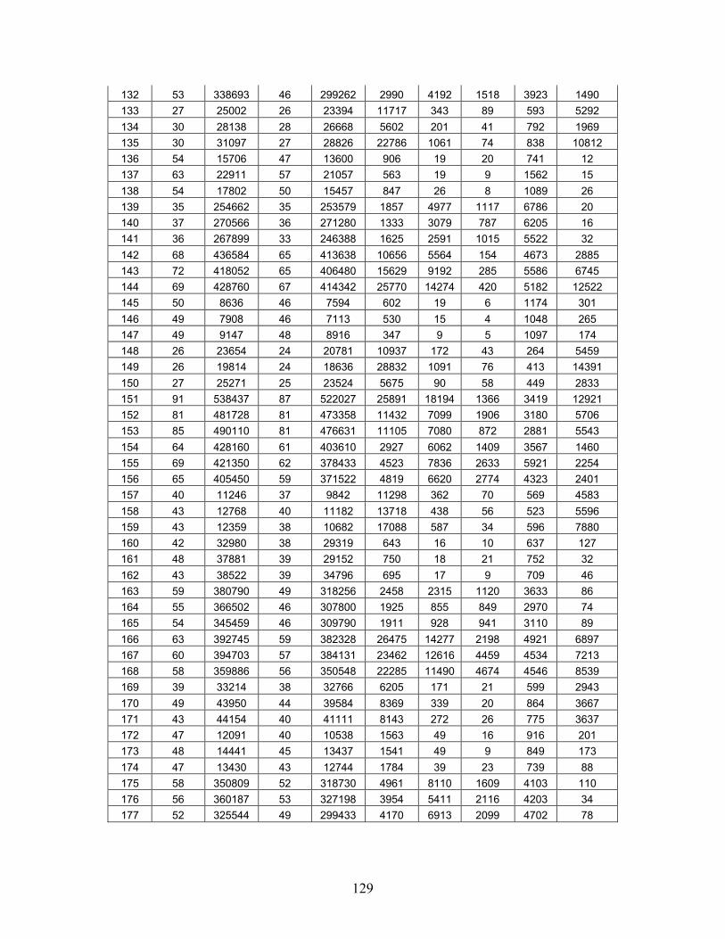
129

132 53 338693 46 299262 2990 4192 1518 3923 1490 133 27 25002 26 23394 11717 343 89 593 5292 134 30 28138 28 26668 5602 201 41 792 1969 135 30 31097 27 28826 22786 1061 74 838 10812 136 54 15706 47 13600 906 19 20 741 12 137 63 22911 57 21057 563 19 9 1562 15 138 54 17802 50 15457 847 26 8 1089 26 139 35 254662 35 253579 1857 4977 1117 6786 20 140 37 270566 36 271280 1333 3079 787 6205 16 141 36 267899 33 246388 1625 2591 1015 5522 32 142 68 436584 65 413638 10656 5564 154 4673 2885 143 72 418052 65 406480 15629 9192 285 5586 6745 144 69 428760 67 414342 25770 14274 420 5182 12522 145 50 8636 46 7594 602 19 6 1174 301 146 49 7908 46 7113 530 15 4 1048 265 147 49 9147 48 8916 347 9 5 1097 174 148 26 23654 24 20781 10937 172 43 264 5459 149 26 19814 24 18636 28832 1091 76 413 14391 150 27 25271 25 23524 5675 90 58 449 2833 151 91 538437 87 522027 25891 18194 1366 3419 12921 152 81 481728 81 473358 11432 7099 1906 3180 5706 153 85 490110 81 476631 11105 7080 872 2881 5543 154 64 428160 61 403610 2927 6062 1409 3567 1460 155 69 421350 62 378433 4523 7836 2633 5921 2254 156 65 405450 59 371522 4819 6620 2774 4323 2401 157 40 11246 37 9842 11298 362 70 569 4583 158 43 12768 40 11182 13718 438 56 523 5596 159 43 12359 38 10682 17088 587 34 596 7880 160 42 32980 38 29319 643 16 10 637 127 161 48 37881 39 29152 750 18 21 752 32 162 43 38522 39 34796 695 17 9 709 46 163 59 380790 49 318256 2458 2315 1120 3633 86 164 55 366502 46 307800 1925 855 849 2970 74 165 54 345459 46 309790 1911 928 941 3110 89 166 63 392745 59 382328 26475 14277 2198 4921 6897 167 60 394703 57 384131 23462 12616 4459 4534 7213 168 58 359886 56 350548 22285 11490 4674 4546 8539 169 39 33214 38 32766 6205 171 21 599 2943 170 49 43950 44 39584 8369 339 20 864 3667 171 43 44154 40 41111 8143 272 26 775 3637 172 47 12091 40 10538 1563 49 16 916 201 173 48 14441 45 13437 1541 49 9 849 173 174 47 13430 43 12744 1784 39 23 739 88 175 58 350809 52 318730 4961 8110 1609 4103 110 176 56 360187 53 327198 3954 5411 2116 4203 34 177 52 325544 49 299433 4170 6913 2099 4702 78

130

178 75 491258 69 471013 10454 5890 850 4917 4253 179 70 475082 67 472023 5373 2883 194 4559 1950 180 70 456738 68 446777 5368 2817 948 4616 2400 181 20 18832 19 17026 1126 10 36 198 563 182 22 16845 18 13900 1537 17 37 231 768 183 21 18673 21 18554 540 7 64 462 270 184 50 8636 50 8636 1511 44 11 1032 753 185 50 8117 50 8117 1511 49 7 1220 753 186 50 9346 50 9346 1511 49 6 1215 753 187 53 378835 51 362222 14671 8277 4958 3493 7308 188 52 354332 51 343410 8189 4954 2856 4364 4080 189 53 348452 52 345083 16892 11705 6355 5171 8417 190 95 576533 91 542598 2264 1661 649 3342 1131 191 88 525069 86 497137 3580 2922 725 3027 1788 192 92 522419 88 494198 2744 1743 888 3127 1371

131

APPENDIX E: Raw Data on Crew Bounds

Design Pt Crew Bound

WT Bound

% Distance ATS

Crews

% Distance ATS WT

% Distance SP

Crews

% Distance SP WT

1 13 11980 0.076923077 0.012520868 0.076923077 0.1059265442 11 8194 0.090909091 0.07773981 0.272727273 0.4475225773 15 10230 0.133333333 0.157673509 0.2 0.65259042 4 29 9083 0 0 0 0.0037432575 28 6063 0 0 0 0 6 30 7968 0 0 0 0.0249749 7 15 119911 0.2 0.136659689 0.333333333 0.3397186258 16 114434 0.125 0.130546865 0.3125 0.3101176229 18 117773 0.055555556 0.111477164 0.222222222 0.40495699410 35 226231 0 0 0 0.00992790611 35 217389 0 0 0 0.01257653312 39 246233 0 0 0 0.01461623713 13 9778 0.076923077 0.065453058 0.076923077 0.14276948314 15 8369 0.2 0.240769507 0.2 0.40518580515 16 8735 0 0.004693761 0.0625 0.15535203216 24 4623 0 0 0 0 17 25 3859 0 0 0 0 18 23 3339 0 0 0 0.00539083619 38 239998 0.052631579 0.075558963 0.078947368 0.15256377120 40 272452 0 0.007865606 0.025 0.08891474521 36 205235 0.055555556 0.12244013 0.138888889 0.22212098322 35 239193 0 0.004749303 0.028571429 0.07011910923 31 199750 0.032258065 0.041822278 0.032258065 0.07804255324 38 246455 0 0.017934308 0 0.05338094225 19 3653 0 0 0 0 26 21 3051 0 0 0 0.03474270727 20 3114 0 0.024084778 0 0.02408477828 16 12665 0 0 0 0.01444927 29 18 10754 0.055555556 0.060070671 0.111111111 0.21052631630 18 9684 0 0 0.055555556 0.13630731131 38 247646 0 0.005964159 0.052631579 0.0730034 32 31 207540 0.032258065 0.043389226 0.064516129 0.09405415833 34 182797 0.058823529 0.048157245 0.058823529 0.24151928134 39 263922 0.051282051 0.063306583 0.051282051 0.11177544935 41 288983 0 0.012976542 0.024390244 0.06397954236 37 237250 0.054054054 0.082524763 0.162162162 0.21002318237 29 9285 0 0 0 0 38 26 5199 0 0 0 0 39 31 9997 0 0 0 0.01760528240 19 19523 0 0.004302617 0 0.02960610641 14 10610 0 0.07464656 0.071428571 0.18925541942 19 15386 0 0.056869882 0 0.25796178343 35 226231 0 0 0 0.009927906

132

44 35 216216 0 0 0 0.01397213945 39 246233 0 0 0 0.01498174546 19 149513 0.210526316 0.12679165 0.315789474 0.22181348847 18 134731 0.111111111 0.077257647 0.222222222 0.20192828748 21 143384 0.095238095 0.168735703 0.142857143 0.25517491549 15 13593 0 0 0.066666667 0.08916354 50 15 9758 0.066666667 0.049087928 0.133333333 0.20362779351 16 10904 0 0.043561996 0 0.04356199652 25 4727 0 0 0 0 53 25 3859 0 0 0 0 54 25 3530 0 0 0 0 55 34 223596 0.058823529 0.092541906 0.088235294 0.18451582356 31 206200 0.064516129 0.133064985 0.193548387 0.37174102857 33 197336 0.060606061 0.167987595 0.181818182 0.40881542158 56 336092 0 0.006736251 0 0.04415457759 55 341093 0 0.000680166 0.018181818 0.03979266760 55 298334 0 0.000157542 0.018181818 0.08960091761 25 23514 0 0 0 0 62 21 14289 0.047619048 0.039121002 0.095238095 0.12821051263 31 24900 0 0 0 0.02365461864 22 4878 0 0 0 0.09963099665 21 3565 0 0 0 0.21739130466 23 4287 0.043478261 0.051317938 0.043478261 0.38021926867 40 242313 0.05 0.058932042 0.1 0.10821128 68 37 234381 0 0.007449409 0.027027027 0.07299653169 40 240184 0.075 0.089548013 0.125 0.18345934870 35 228176 0 0 0 0.00864245171 32 208743 0 0 0 0.01114288972 38 214130 0 0 0 0.01260916373 29 9517 0 0 0 0 74 25 5695 0 0 0 0.02546093175 31 11054 0 0 0 0.02876786776 23 22142 0.043478261 0.030123747 0.043478261 0.05943455977 18 12335 0.111111111 0.092257803 0.111111111 0.19181191778 28 24421 0 0 0 0.01998280279 44 277216 0 0 0 0.01164795780 38 252911 0 0 0 0.01127669481 44 263109 0 0 0 0.0145339 82 35 212292 0.085714286 0.105887174 0.142857143 0.17184349983 32 189460 0.03125 0.058175868 0.09375 0.21090467684 34 202410 0.147058824 0.119860679 0.235294118 0.26978904285 25 4727 0 0 0 0 86 25 3859 0 0 0 0 87 25 3530 0 0 0 0 88 12 11499 0 0 0.083333333 0.10913992589 13 9376 0.076923077 0.051087884 0.153846154 0.22088310690 14 9408 0 0.06122449 0 0.06122449 91 52 318899 0 0.000310443 0.019230769 0.07333983592 53 339247 0 0.010367078 0.018867925 0.05868880293 53 312592 0 0.001247633 0.018867925 0.04494676894 34 226659 0.147058824 0.207990859 0.147058824 0.24582302

133

95 34 237677 0.088235294 0.131910113 0.205882353 0.27853347296 36 222363 0 0.065577457 0.083333333 0.23877623597 57 13835 0 0 0 0 98 52 11470 0 0 0 0.08047079399 52 12158 0 0 0 0.087761145

100 26 21538 0.038461538 0.085987557 0.153846154 0.316788931101 22 17573 0.181818182 0.215045809 0.454545455 0.631024868102 24 24060 0.041666667 0.053283458 0.291666667 0.312635079103 68 436584 0 0 0 0.010918861104 72 424930 0 0 0 0.013981126105 69 428980 0 0 0 0.011263928106 21 158447 0.285714286 0.282447759 0.571428571 0.581399458107 27 189568 0.111111111 0.168504178 0.37037037 0.452164922108 26 178301 0.153846154 0.18558505 0.307692308 0.383149842109 43 8062 0 0 0 0 110 45 7743 0 0 0 0.003487021111 48 9286 0 0 0 0 112 28 19631 0.071428571 0.136620651 0.178571429 0.297947124113 28 17450 0.035714286 0.075873926 0.035714286 0.202234957114 28 22419 0.107142857 0.063874392 0.285714286 0.313484098115 69 457963 0.043478261 0.050130687 0.086956522 0.115225466116 66 393006 0.03030303 0.103390279 0.03030303 0.143944367117 66 400261 0.045454545 0.070056788 0.045454545 0.146594347118 52 313329 0.134615385 0.179300352 0.192307692 0.327470486119 50 266393 0.18 0.301355516 0.26 0.477140916120 49 252305 0.102040816 0.25408137 0.183673469 0.408307406121 30 21466 0 0.082269636 0.066666667 0.161418056122 31 20858 0.032258065 0.029101544 0.032258065 0.101543772123 33 26636 0.03030303 0.029508935 0.060606061 0.084810032124 34 6606 0 0 0 0.040720557125 33 5915 0 0 0 0.064243449126 36 7726 0 0 0 0.00673052 127 69 437738 0.028985507 0.034666856 0.086956522 0.140999868128 70 413047 0.014285714 0.043902994 0.042857143 0.122533271129 63 371023 0.031746032 0.062149786 0.095238095 0.174986456130 52 347689 0.096153846 0.105588615 0.192307692 0.235638746131 53 310388 0.018867925 0.08515471 0.037735849 0.200809954132 51 314215 0.039215686 0.077902073 0.039215686 0.154381554133 26 23732 0.038461538 0.053514242 0.115384615 0.157677398134 26 23952 0.153846154 0.174766199 0.307692308 0.358132933135 29 30984 0.034482759 0.003647044 0.206896552 0.22669765 136 54 15706 0 0 0 0.024640265137 63 22911 0 0 0.015873016 0.017022391138 54 17802 0 0 0 0.006010561139 30 206209 0.166666667 0.234970346 0.366666667 0.557419899140 34 239814 0.088235294 0.128232714 0.264705882 0.293335668141 33 234735 0.090909091 0.141282723 0.212121212 0.313370396142 68 436584 0 0 0 0.011743445143 72 418052 0 0 0 0.015526777144 69 428760 0 0 0 0.011689523145 50 8636 0 0 0 0

134

146 49 7908 0 0 0 0 147 49 9147 0 0 0 0 148 25 22083 0.04 0.071140696 0.04 0.090069284149 24 19372 0.083333333 0.022816436 0.083333333 0.116405121150 27 25271 0 0 0.148148148 0.184955087151 91 532356 0 0.011422807 0 0.041203631152 81 468504 0 0.028226013 0.012345679 0.058012312153 85 475749 0 0.030186086 0 0.070476239154 55 351159 0.163636364 0.219276738 0.236363636 0.377265 155 63 370244 0.095238095 0.138033297 0.174603175 0.28349953 156 60 361515 0.083333333 0.121530227 0.15 0.282168098157 40 11084 0 0.014615662 0.025 0.061349693158 42 12541 0.023809524 0.01810063 0.023809524 0.090662627159 43 12351 0 0.000647721 0 0.040725447160 41 32666 0.024390244 0.009612441 0.048780488 0.060460418161 48 37343 0 0.014406984 0 0.041399995162 43 38522 0 0 0.046511628 0.122345673163 59 380790 0 0 0 0.014349116164 55 366502 0 0 0 0.013372369165 54 345459 0 0 0 0.014959807166 57 342380 0.105263158 0.147102634 0.157894737 0.274586717167 58 378528 0.034482759 0.042731317 0.068965517 0.154775869168 54 323767 0.074074074 0.111558621 0.148148148 0.23148437 169 38 32543 0.026315789 0.020618873 0.105263158 0.123805427170 49 43950 0 0 0.020408163 0.093219568171 42 43917 0.023809524 0.005396543 0.071428571 0.067536489172 47 12091 0 0 0 0.037135059173 48 14372 0 0.004801002 0.020833333 0.145978291174 47 13286 0 0.010838477 0 0.118846907175 51 304716 0.137254902 0.151265441 0.196078431 0.311890416176 53 338244 0.056603774 0.064873287 0.132075472 0.187231703177 48 289706 0.083333333 0.123704721 0.229166667 0.275061614178 75 491258 0 0 0 0.013469501179 70 475082 0 0 0 0.010979157180 70 456738 0 0 0 0.015124645181 20 18291 0 0.029577388 0.05 0.085506533182 21 16402 0.047619048 0.027008901 0.047619048 0.109376905183 19 17398 0.105263158 0.073284286 0.315789474 0.391884125184 50 8636 0 0 0 0 185 50 8117 0 0 0 0 186 50 9346 0 0 0 0 187 42 274204 0.261904762 0.381580867 0.285714286 0.456685533188 46 302908 0.130434783 0.169767718 0.173913043 0.263892007189 42 258787 0.261904762 0.346481856 0.333333333 0.475139787190 95 575748 0 0.001363444 0.010526316 0.039366181191 88 525046 0 4.38057E-05 0.011363636 0.040379319192 92 519702 0 0.005227996 0.010869565 0.065260476

135

APPENDIX F: Example TCSP Bound Solution

Arcs in the solution: X0-1,1.0 X1-21,1.0 X0-2,1.0 X2-5,1.0 X0-3,1.0 X3-9,1.0 X0-4,1.0 X4-12,1.0 X5-13,1.0 X0-6,1.0 X6-27,1.0 X0-7,1.0 X7-16,1.0 X0-8,1.0 X8-18,1.0 X0-10,1.0 X10-25,1.0 X0-11,1.0 X11-19,1.0 X12-20,1.0 X0-14,1.0 X14-26,1.0 X0-15,1.0 X15-24,1.0 X16-22,1.0 X0-17,1.0 X21-29,1.0 X22-28,1.0 X0-23,1.0 X25-30,1.0 The cost is: 1.300001198E10

136

APPENDIX G: ANOVA Calculations for the Designed Experiment Analysis of Variance for ATS Crews Source DF Seq SS Adj SS Adj MS F P Rot/day 1 21781.4 21781.4 21781.4 671.38 0.000 numBase 1 1604.3 1604.3 1604.3 49.45 0.000 TBF 1 9.6 9.6 9.6 0.30 0.587 TBR 1 0.6 0.6 0.6 0.02 0.889 numDIS 1 17652.5 17652.5 17652.5 544.12 0.000 PCF 1 0.4 0.4 0.4 0.01 0.909 ISGS 1 2.8 2.8 2.8 0.08 0.771 CP 1 11.5 11.5 11.5 0.35 0.552 MDIBN 1 159.5 159.5 159.5 4.92 0.028 RS 1 2921.9 2921.9 2921.9 90.06 0.000 RT 1 4971.5 4971.5 4971.5 153.24 0.000 RDT 1 6996.3 6996.3 6996.3 215.65 0.000 MWBF 1 764.0 764.0 764.0 23.55 0.000 tenure 1 10.5 10.5 10.5 0.33 0.569 C/I 1 7.9 7.9 7.9 0.24 0.622 Error 176 5709.9 5709.9 32.4 Total 191 62604.6 Analysis of Variance for ATS WT Source DF Seq SS Adj SS Adj MS F P Rot/day 1 3.1894E+11 3.1894E+11 3.1894E+11 112.25 0.000 numBase 1 3.6354E+10 3.6354E+10 3.6354E+10 12.79 0.000 TBF 1 1637413378 1637413378 1637413378 0.58 0.449 TBR 1 1153045 1153045 1153045 0.00 0.984 numDIS 1 4.3850E+12 4.3850E+12 4.3850E+12 1543.32 0.000 PCF 1 24918493 24918493 24918493 0.01 0.925 ISGS 1 412687798 412687798 412687798 0.15 0.704 CP 1 1.6620E+10 1.6620E+10 1.6620E+10 5.85 0.017 MDIBN 1 6201801101 6201801101 6201801101 2.18 0.141 RS 1 4.9041E+10 4.9041E+10 4.9041E+10 17.26 0.000 RT 1 4.2557E+10 4.2557E+10 4.2557E+10 14.98 0.000 RDT 1 3.3708E+10 3.3708E+10 3.3708E+10 11.86 0.001 MWBF 1 1.7412E+10 1.7412E+10 1.7412E+10 6.13 0.014 tenure 1 81019931 81019931 81019931 0.03 0.866 C/I 1 3784878001 3784878001 3784878001 1.33 0.250 Error 176 5.0006E+11 5.0006E+11 2841273781 Total 191 5.4118E+12 Analysis of Variance for ATS Near feasible Crews Source DF Seq SS Adj SS Adj MS F P Rot/day 1 19180.0 19180.0 19180.0 624.75 0.000 numBase 1 1349.4 1349.4 1349.4 43.95 0.000 TBF 1 12.5 12.5 12.5 0.41 0.524 TBR 1 1.9 1.9 1.9 0.06 0.805

137

numDIS 1 16856.3 16856.3 16856.3 549.06 0.000 PCF 1 1.9 1.9 1.9 0.06 0.805 ISGS 1 0.0 0.0 0.0 0.00 0.990 CP 1 9.6 9.6 9.6 0.31 0.576 MDIBN 1 231.9 231.9 231.9 7.55 0.007 RS 1 2501.3 2501.3 2501.3 81.48 0.000 RT 1 5450.7 5450.7 5450.7 177.55 0.000 RDT 1 6521.7 6521.7 6521.7 212.43 0.000 MWBF 1 1135.9 1135.9 1135.9 37.00 0.000 tenure 1 10.5 10.5 10.5 0.34 0.559 C/I 1 86.7 86.7 86.7 2.82 0.095 Error 176 5403.2 5403.2 30.7 Total 191 58753.4 Analysis of Variance for ATS Near feasible Wait Time Source DF Seq SS Adj SS Adj MS F P Rot/day 1 2.9877E+11 2.9877E+11 2.9877E+11 106.96 0.000 numBase 1 3.0056E+10 3.0056E+10 3.0056E+10 10.76 0.001 TBF 1 1398686576 1398686576 1398686576 0.50 0.480 TBR 1 106943596 106943596 106943596 0.04 0.845 numDIS 1 3.9280E+12 3.9280E+12 3.9280E+12 1406.29 0.000 PCF 1 52310664 52310664 52310664 0.02 0.891 ISGS 1 555846020 555846020 555846020 0.20 0.656 CP 1 1.4012E+10 1.4012E+10 1.4012E+10 5.02 0.026 MDIBN 1 8723447252 8723447252 8723447252 3.12 0.079 RS 1 4.0127E+10 4.0127E+10 4.0127E+10 14.37 0.000 RT 1 4.8433E+10 4.8433E+10 4.8433E+10 17.34 0.000 RDT 1 3.2941E+10 3.2941E+10 3.2941E+10 11.79 0.001 MWBF 1 2.6836E+10 2.6836E+10 2.6836E+10 9.61 0.002 tenure 1 103858484 103858484 103858484 0.04 0.847 C/I 1 1.1601E+10 1.1601E+10 1.1601E+10 4.15 0.043 Error 176 4.9160E+11 4.9160E+11 2793168536 Total 191 4.9333E+12 Analysis of Variance for Iterations Source DF Seq SS Adj SS Adj MS F P Rot/day 1 233866967 233866967 233866967 12.37 0.001 numBase 1 47314 47314 47314 0.00 0.960 TBF 1 1922001 1922001 1922001 0.10 0.750 TBR 1 2581 2581 2581 0.00 0.991 numDIS 1 709748555 709748555 709748555 37.53 0.000 PCF 1 24795438 24795438 24795438 1.31 0.254 ISGS 1 664555717 664555717 664555717 35.14 0.000 CP 1 10187183 10187183 10187183 0.54 0.464 MDIBN 1 1841225 1841225 1841225 0.10 0.755 RS 1 71109311 71109311 71109311 3.76 0.054 RT 1 15638550 15638550 15638550 0.83 0.364 RDT 1 188159401 188159401 188159401 9.95 0.002 MWBF 1 6483435 6483435 6483435 0.34 0.559 tenure 1 12696833 12696833 12696833 0.67 0.414 C/I 1 3434709279 3434709279 3434709279 181.64 0.000 Error 176 3328118071 3328118071 18909762 Total 191 8703881857

138

Analysis of Variance for Total Solution Time (TST) Source DF Seq SS Adj SS Adj MS F P Rot/day 1 385188847 385188847 385188847 43.72 0.000 numBase 1 2109456 2109456 2109456 0.24 0.625 TBF 1 4285569 4285569 4285569 0.49 0.486 TBR 1 3473597 3473597 3473597 0.39 0.531 numDIS 1 808360779 808360779 808360779 91.75 0.000 PCF 1 820718 820718 820718 0.09 0.761 ISGS 1 51911600 51911600 51911600 5.89 0.016 CP 1 32514261 32514261 32514261 3.69 0.056 MDIBN 1 52041 52041 52041 0.01 0.939 RS 1 21614923 21614923 21614923 2.45 0.119 RT 1 21085391 21085391 21085391 2.39 0.124 RDT 1 81009538 81009538 81009538 9.20 0.003 MWBF 1 13052 13052 13052 0.00 0.969 tenure 1 14812408 14812408 14812408 1.68 0.196 C/I 1 136692563 136692563 136692563 15.52 0.000 Error 176 1550561940 1550561940 8810011 Total 191 3114506682 Analysis of Variance for Number of Conjugacy Classes Visited Source DF Seq SS Adj SS Adj MS F P Rot/day 1 5264888 5264888 5264888 3.35 0.069 numBase 1 188376 188376 188376 0.12 0.730 TBF 1 562034 562034 562034 0.36 0.550 TBR 1 181425 181425 181425 0.12 0.734 numDIS 1 145812408 145812408 145812408 92.83 0.000 PCF 1 2006963 2006963 2006963 1.28 0.260 ISGS 1 1549445 1549445 1549445 0.99 0.322 CP 1 14210369 14210369 14210369 9.05 0.003 MDIBN 1 1010360 1010360 1010360 0.64 0.424 RS 1 7524792 7524792 7524792 4.79 0.030 RT 1 10617305 10617305 10617305 6.76 0.010 RDT 1 23888230 23888230 23888230 15.21 0.000 MWBF 1 1531888 1531888 1531888 0.98 0.325 tenure 1 2104219 2104219 2104219 1.34 0.249 C/I 1 19797999 19797999 19797999 12.60 0.000 Error 176 276448966 276448966 1570733 Total 191 512699666 Analysis of Variance for Average Neighborhood Size Source DF Seq SS Adj SS Adj MS F P Rot/day 1 171015050 171015050 171015050 211.27 0.000 numBase 1 9284002 9284002 9284002 11.47 0.001 TBF 1 166852 166852 166852 0.21 0.650 TBR 1 27792 27792 27792 0.03 0.853 numDIS 1 335386133 335386133 335386133 414.33 0.000 PCF 1 183521 183521 183521 0.23 0.635 ISGS 1 1022292 1022292 1022292 1.26 0.263 CP 1 1249365 1249365 1249365 1.54 0.216 MDIBN 1 660352 660352 660352 0.82 0.368

139

RS 1 20378 20378 20378 0.03 0.874 RT 1 120501 120501 120501 0.15 0.700 RDT 1 1075205 1075205 1075205 1.33 0.251 MWBF 1 2121002 2121002 2121002 2.62 0.107 tenure 1 560520 560520 560520 0.69 0.406 C/I 1 869678 869678 869678 1.07 0.301 Error 176 142465887 142465887 809465 Total 191 666228531 Analysis of Variance for Average Tenure Source DF Seq SS Adj SS Adj MS F P Rot/day 1 51046875 51046875 51046875 12.28 0.001 numBase 1 250274 250274 250274 0.06 0.806 TBF 1 5852 5852 5852 0.00 0.970 TBR 1 244816 244816 244816 0.06 0.809 numDIS 1 86028075 86028075 86028075 20.70 0.000 PCF 1 2916588 2916588 2916588 0.70 0.403 ISGS 1 104270761 104270761 104270761 25.09 0.000 CP 1 19120 19120 19120 0.00 0.946 MDIBN 1 664581 664581 664581 0.16 0.690 RS 1 13005213 13005213 13005213 3.13 0.079 RT 1 1426920 1426920 1426920 0.34 0.559 RDT 1 27700485 27700485 27700485 6.66 0.011 MWBF 1 778771 778771 778771 0.19 0.666 tenure 1 26082431 26082431 26082431 6.28 0.013 C/I 1 813231049 813231049 813231049 195.66 0.000 Error 176 731527053 731527053 4156404 Total 191 1859198864

Estimated Effects and Coefficients for ATS CREWS(coded units) Term Effect Coef SE Coef T P Constant 40.151 0.1739 230.88 0.000 Rot/day 21.302 10.651 0.1739 61.25 0.000 num_Base 5.781 2.891 0.1739 16.62 0.000 TBF 0.448 0.224 0.1739 1.29 0.200 TBR -0.115 -0.057 0.1739 -0.33 0.742 num_DIS 19.177 9.589 0.1739 55.14 0.000 PCF 0.094 0.047 0.1739 0.27 0.788 ISGS -0.240 -0.120 0.1739 -0.69 0.492 CP 0.490 0.245 0.1739 1.41 0.162 MDIBN 1.823 0.911 0.1739 5.24 0.000 RS 7.802 3.901 0.1739 22.43 0.000 RT 10.177 5.089 0.1739 29.26 0.000 RDT 12.073 6.036 0.1739 34.71 0.000 MWBF 3.990 1.995 0.1739 11.47 0.000 tenure 0.469 0.234 0.1739 1.35 0.180 C/I -0.406 -0.203 0.1739 -1.17 0.245 Rot/day*num_Base 0.531 0.266 0.1739 1.53 0.129 Rot/day*TBF -0.177 -0.089 0.1739 -0.51 0.611 Rot/day*TBR 0.010 0.005 0.1739 0.03 0.976 Rot/day*num_DIS 3.510 1.755 0.1739 10.09 0.000 Rot/day*PCF 0.260 0.130 0.1739 0.75 0.455 Rot/day*ISGS 2.385 1.193 0.1739 6.86 0.000

140

Rot/day*CP 0.531 0.266 0.1739 1.53 0.129 Rot/day*MDIBN 1.240 0.620 0.1739 3.56 0.001 Rot/day*RS 1.802 0.901 0.1739 5.18 0.000 Rot/day*RT 3.052 1.526 0.1739 8.78 0.000 Rot/day*RDT 4.781 2.391 0.1739 13.75 0.000 Rot/day*MWBF 2.156 1.078 0.1739 6.20 0.000 Rot/day*tenure 2.302 1.151 0.1739 6.62 0.000 Rot/day*C/I -0.073 -0.036 0.1739 -0.21 0.834 num_Base*TBF 0.052 0.026 0.1739 0.15 0.881 num_Base*TBR -2.177 -1.089 0.1739 -6.26 0.000 num_Base*num_DIS 3.948 1.974 0.1739 11.35 0.000 num_Base*ISGS -1.010 -0.505 0.1739 -2.91 0.004 num_Base*CP -0.281 -0.141 0.1739 -0.81 0.420 num_Base*MDIBN 0.219 0.109 0.1739 0.63 0.530 num_Base*RS 0.365 0.182 0.1739 1.05 0.296 num_Base*RT -0.552 -0.276 0.1739 -1.59 0.115 num_Base*RDT -0.740 -0.370 0.1739 -2.13 0.035 num_Base*tenure 0.656 0.328 0.1739 1.89 0.061 num_Base*C/I -0.344 -0.172 0.1739 -0.99 0.325 TBF*TBR -0.677 -0.339 0.1739 -1.95 0.054 TBF*num_DIS 0.490 0.245 0.1739 1.41 0.162 TBF*ISGS 0.656 0.328 0.1739 1.89 0.061 TBF*RS 0.073 0.036 0.1739 0.21 0.834 TBF*RT 0.281 0.141 0.1739 0.81 0.420 TBF*tenure -1.135 -0.568 0.1739 -3.26 0.001 TBF*C/I -1.635 -0.818 0.1739 -4.70 0.000 TBR*num_DIS -0.406 -0.203 0.1739 -1.17 0.245 TBR*RS -0.198 -0.099 0.1739 -0.57 0.570 TBR*tenure 0.094 0.047 0.1739 0.27 0.788 TBR*C/I 1.427 0.714 0.1739 4.10 0.000 num_DIS*C/I -1.740 -0.870 0.1739 -5.00 0.000 ISGS*RS -0.615 -0.307 0.1739 -1.77 0.080 ISGS*RDT 0.448 0.224 0.1739 1.29 0.200 ISGS*MWBF -0.302 -0.151 0.1739 -0.87 0.387 CP*RS -0.510 -0.255 0.1739 -1.47 0.145 CP*MWBF 0.010 0.005 0.1739 0.03 0.976 MDIBN*RS 1.698 0.849 0.1739 4.88 0.000 Analysis of Variance for ATS (coded units) Source DF Seq SS Adj SS Adj MS F P Main Effects 15 56894.7 56894.7 3792.98 653.22 0.000 2-Way Interactions 43 4937.6 4937.6 114.83 19.78 0.000 Residual Error 133 772.3 772.3 5.81 Lack of Fit 5 24.3 24.3 4.86 0.83 0.530 Pure Error 128 748.0 748.0 5.84 Total 191 62604.6 Unusual Observations for ATS _ cr Obs ATS _ cr Fit SE Fit Residual St Resid 62 22.0000 26.4531 1.3358 -4.4531 -2.22R 63 31.0000 26.4531 1.3358 4.5469 2.27R 78 28.0000 23.2656 1.3358 4.7344 2.36R 80 38.0000 42.5156 1.3358 -4.5156 -2.25R 137 63.0000 56.5990 1.3358 6.4010 3.19R

141

151 91.0000 85.2656 1.3358 5.7344 2.86R 152 81.0000 85.2656 1.3358 -4.2656 -2.13R 169 39.0000 44.1823 1.3358 -5.1823 -2.58R 170 49.0000 44.1823 1.3358 4.8177 2.40R 178 75.0000 70.9323 1.3358 4.0677 2.03R R denotes an observation with a large standardized residual Estimated Effects and Coefficients for ATS Wait Time(coded units) Term Effect Coef SE Coef T P Constant 165491 991.1 166.97 0.000 Rot/day 81514 40757 991.1 41.12 0.000 num_Base 27520 13760 991.1 13.88 0.000 TBF 5841 2920 991.1 2.95 0.004 TBR -155 -77 991.1 -0.08 0.938 num_DIS 302248 151124 991.1 152.48 0.000 PCF 721 360 991.1 0.36 0.717 ISGS 2932 1466 991.1 1.48 0.141 CP 18608 9304 991.1 9.39 0.000 MDIBN 11367 5683 991.1 5.73 0.000 RS 31964 15982 991.1 16.12 0.000 RT 29776 14888 991.1 15.02 0.000 RDT 26500 13250 991.1 13.37 0.000 MWBF 19046 9523 991.1 9.61 0.000 tenure 1299 650 991.1 0.66 0.513 C/I -8880 -4440 991.1 -4.48 0.000 Rot/day*num_Base 3839 1919 991.1 1.94 0.055 Rot/day*TBF 607 304 991.1 0.31 0.760 Rot/day*TBR -1732 -866 991.1 -0.87 0.384 Rot/day*num_DIS 72225 36113 991.1 36.44 0.000 Rot/day*PCF 4 2 991.1 0.00 0.998 Rot/day*ISGS 26319 13160 991.1 13.28 0.000 Rot/day*CP 38562 19281 991.1 19.45 0.000 Rot/day*MDIBN 17950 8975 991.1 9.06 0.000 Rot/day*RS 3027 1514 991.1 1.53 0.129 Rot/day*RT 4240 2120 991.1 2.14 0.034 Rot/day*RDT 14928 7464 991.1 7.53 0.000 Rot/day*MWBF 10840 5420 991.1 5.47 0.000 Rot/day*tenure 25443 12722 991.1 12.84 0.000 Rot/day*C/I -2053 -1026 991.1 -1.04 0.302 num_Base*TBF 120 60 991.1 0.06 0.952 num_Base*TBR -6197 -3099 991.1 -3.13 0.002 num_Base*num_DIS 25592 12796 991.1 12.91 0.000 num_Base*ISGS -3173 -1586 991.1 -1.60 0.112 num_Base*CP -3281 -1640 991.1 -1.66 0.100 num_Base*MDIBN 748 374 991.1 0.38 0.707 num_Base*RS 455 227 991.1 0.23 0.819 num_Base*RT -8361 -4180 991.1 -4.22 0.000 num_Base*RDT -52 -26 991.1 -0.03 0.979 num_Base*tenure 1431 715 991.1 0.72 0.472 num_Base*C/I -1006 -503 991.1 -0.51 0.613 TBF*TBR -1548 -774 991.1 -0.78 0.436 TBF*num_DIS 4550 2275 991.1 2.30 0.023

142

TBF*ISGS 4556 2278 991.1 2.30 0.023 TBF*RS -4354 -2177 991.1 -2.20 0.030 TBF*RT -569 -285 991.1 -0.29 0.774 TBF*tenure -4775 -2388 991.1 -2.41 0.017 TBF*C/I -10133 -5067 991.1 -5.11 0.000 TBR*num_DIS -160 -80 991.1 -0.08 0.936 TBR*RS 1059 530 991.1 0.53 0.594 TBR*tenure 161 80 991.1 0.08 0.936 TBR*C/I 2583 1292 991.1 1.30 0.195 num_DIS*C/I -8853 -4426 991.1 -4.47 0.000 ISGS*RS -3709 -1854 991.1 -1.87 0.064 ISGS*RDT 2193 1096 991.1 1.11 0.271 ISGS*MWBF -4108 -2054 991.1 -2.07 0.040 CP*RS -2787 -1394 991.1 -1.41 0.162 CP*MWBF 634 317 991.1 0.32 0.750 MDIBN*RS 5785 2892 991.1 2.92 0.004 Analysis of Variance for ATS (coded units) Source DF Seq SS Adj SS Adj MS F P Main Effects 15 4.91176E+12 4.9118E+12 3.2745E+11 2E+03 0.000 2-Way Interactions 43 4.74979E+11 4.7498E+11 1.1046E+10 58.57 0.000 Residual Error 133 25085081634 2.5085E+10 188609636 Lack of Fit 5 948762311 948762311 189752462 1.01 0.417 Pure Error 128 24136319323 2.4136E+10 188564995 Total 191 5.41182E+12 Unusual Observations for ATS WT Obs ATS WT Fit SE Fit Residual St Resid 20 274595 250568 7613 24027 2.10R 23 208104 231133 7613 -23029 -2.01R 31 249123 217430 7613 31693 2.77R 33 191600 217430 7613 -25830 -2.26R 60 298381 329460 7613 -31079 -2.72R 96 236945 261941 7613 -24996 -2.19R 115 480921 449599 7613 31322 2.74R 120 316411 347984 7613 -31573 -2.76R 127 452913 425901 7613 27012 2.36R 129 394082 425901 7613 -31819 -2.78R 130 384401 354955 7613 29446 2.58R 151 538437 499995 7613 38442 3.36R 190 576533 541142 7613 35391 3.10R R denotes an observation with a large standardized residual Estimated Effects and Coefficients for ATS Near feasible Crews Term Effect Coef SE Coef T P Constant 37.557 0.1468 255.76 0.000 Rot/day 19.990 9.995 0.1468 68.06 0.000 num_Base 5.302 2.651 0.1468 18.05 0.000 TBF 0.510 0.255 0.1468 1.74 0.085 TBR -0.198 -0.099 0.1468 -0.67 0.502 num_DIS 18.740 9.370 0.1468 63.81 0.000

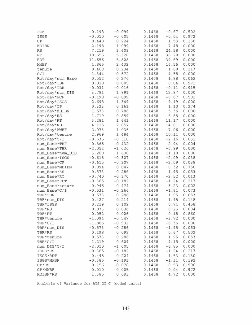
143

PCF -0.198 -0.099 0.1468 -0.67 0.502 ISGS -0.010 -0.005 0.1468 -0.04 0.972 CP 0.448 0.224 0.1468 1.53 0.130 MDIBN 2.198 1.099 0.1468 7.48 0.000 RS 7.219 3.609 0.1468 24.58 0.000 RT 10.656 5.328 0.1468 36.28 0.000 RDT 11.656 5.828 0.1468 39.69 0.000 MWBF 4.865 2.432 0.1468 16.56 0.000 tenure 0.469 0.234 0.1468 1.60 0.113 C/I -1.344 -0.672 0.1468 -4.58 0.000 Rot/day*num_Base 0.552 0.276 0.1468 1.88 0.062 Rot/day*TBF 0.010 0.005 0.1468 0.04 0.972 Rot/day*TBR -0.031 -0.016 0.1468 -0.11 0.915 Rot/day*num_DIS 3.781 1.891 0.1468 12.87 0.000 Rot/day*PCF -0.198 -0.099 0.1468 -0.67 0.502 Rot/day*ISGS 2.698 1.349 0.1468 9.19 0.000 Rot/day*CP 0.323 0.161 0.1468 1.10 0.274 Rot/day*MDIBN 1.573 0.786 0.1468 5.36 0.000 Rot/day*RS 1.719 0.859 0.1468 5.85 0.000 Rot/day*RT 3.281 1.641 0.1468 11.17 0.000 Rot/day*RDT 4.115 2.057 0.1468 14.01 0.000 Rot/day*MWBF 2.073 1.036 0.1468 7.06 0.000 Rot/day*tenure 2.969 1.484 0.1468 10.11 0.000 Rot/day*C/I -0.635 -0.318 0.1468 -2.16 0.032 num_Base*TBF 0.865 0.432 0.1468 2.94 0.004 num_Base*TBR -2.052 -1.026 0.1468 -6.99 0.000 num_Base*num_DIS 3.260 1.630 0.1468 11.10 0.000 num_Base*ISGS -0.615 -0.307 0.1468 -2.09 0.038 num_Base*CP -0.615 -0.307 0.1468 -2.09 0.038 num_Base*MDIBN 0.094 0.047 0.1468 0.32 0.750 num_Base*RS 0.573 0.286 0.1468 1.95 0.053 num_Base*RT -0.740 -0.370 0.1468 -2.52 0.013 num_Base*RDT -0.365 -0.182 0.1468 -1.24 0.217 num_Base*tenure 0.948 0.474 0.1468 3.23 0.002 num_Base*C/I -0.531 -0.266 0.1468 -1.81 0.073 TBF*TBR 0.573 0.286 0.1468 1.95 0.053 TBF*num_DIS 0.427 0.214 0.1468 1.45 0.148 TBF*ISGS 0.219 0.109 0.1468 0.74 0.458 TBF*RS 0.073 0.036 0.1468 0.25 0.804 TBF*RT 0.052 0.026 0.1468 0.18 0.860 TBF*tenure -1.094 -0.547 0.1468 -3.72 0.000 TBF*C/I -1.865 -0.932 0.1468 -6.35 0.000 TBR*num_DIS -0.573 -0.286 0.1468 -1.95 0.053 TBR*RS 0.198 0.099 0.1468 0.67 0.502 TBR*tenure 0.573 0.286 0.1468 1.95 0.053 TBR*C/I 1.219 0.609 0.1468 4.15 0.000 num_DIS*C/I -2.010 -1.005 0.1468 -6.85 0.000 ISGS*RS -0.365 -0.182 0.1468 -1.24 0.217 ISGS*RDT 0.448 0.224 0.1468 1.53 0.130 ISGS*MWBF -0.385 -0.193 0.1468 -1.31 0.192 CP*RS -0.156 -0.078 0.1468 -0.53 0.596 CP*MWBF -0.010 -0.005 0.1468 -0.04 0.972 MDIBN*RS 1.385 0.693 0.1468 4.72 0.000 Analysis of Variance for ATS_GI_C (coded units)

144

Source DF Seq SS Adj SS Adj MS F P Main Effects 15 53350.2 53350.2 3556.68 859.05 0.000 2-Way Interactions 43 4852.6 4852.6 112.85 27.26 0.000 Residual Error 133 550.7 550.7 4.14 Lack of Fit 5 15.3 15.3 3.06 0.73 0.600 Pure Error 128 535.3 535.3 4.18 Total 191 58753.4 Unusual Observations for ATS_GI_C Obs ATS_GI_C Fit SE Fit Residual St Resid 32 27.0000 30.8802 1.1279 -3.8802 -2.29R 62 20.0000 24.4427 1.1279 -4.4427 -2.62R 63 29.0000 24.4427 1.1279 4.5573 2.69R 74 22.0000 26.1094 1.1279 -4.1094 -2.43R 75 30.0000 26.1094 1.1279 3.8906 2.30R 80 37.0000 40.4427 1.1279 -3.4427 -2.03R 125 27.0000 30.4427 1.1279 -3.4427 -2.03R 136 47.0000 51.0677 1.1279 -4.0677 -2.40R 137 57.0000 51.0677 1.1279 5.9323 3.50R 151 87.0000 82.7344 1.1279 4.2656 2.52R R denotes an observation with a large standardized residual Estimated Effects and Coefficients for ATS Near feasible Wait Time Term Effect Coef SE Coef T P Constant 156037 861.1 181.20 0.000 Rot/day 78895 39447 861.1 45.81 0.000 num_Base 25023 12512 861.1 14.53 0.000 TBF 5398 2699 861.1 3.13 0.002 TBR -1493 -746 861.1 -0.87 0.388 num_DIS 286065 143033 861.1 166.10 0.000 PCF -1044 -522 861.1 -0.61 0.545 ISGS 3403 1701 861.1 1.98 0.050 CP 17086 8543 861.1 9.92 0.000 MDIBN 13481 6741 861.1 7.83 0.000 RS 28913 14457 861.1 16.79 0.000 RT 31765 15883 861.1 18.44 0.000 RDT 26197 13098 861.1 15.21 0.000 MWBF 23645 11822 861.1 13.73 0.000 tenure 1471 735 861.1 0.85 0.395 C/I -15546 -7773 861.1 -9.03 0.000 Rot/day*num_Base 2156 1078 861.1 1.25 0.213 Rot/day*TBF 1258 629 861.1 0.73 0.466 Rot/day*TBR -1223 -611 861.1 -0.71 0.479 Rot/day*num_DIS 70556 35278 861.1 40.97 0.000 Rot/day*PCF -2349 -1175 861.1 -1.36 0.175 Rot/day*ISGS 28634 14317 861.1 16.63 0.000 Rot/day*CP 36904 18452 861.1 21.43 0.000 Rot/day*MDIBN 22271 11135 861.1 12.93 0.000 Rot/day*RS 2845 1423 861.1 1.65 0.101 Rot/day*RT 4731 2365 861.1 2.75 0.007 Rot/day*RDT 13631 6815 861.1 7.91 0.000

145

Rot/day*MWBF 12712 6356 861.1 7.38 0.000 Rot/day*tenure 23410 11705 861.1 13.59 0.000 Rot/day*C/I -4992 -2496 861.1 -2.90 0.004 num_Base*TBF 2915 1458 861.1 1.69 0.093 num_Base*TBR -6361 -3180 861.1 -3.69 0.000 num_Base*num_DIS 23125 11562 861.1 13.43 0.000 num_Base*ISGS -2101 -1050 861.1 -1.22 0.225 num_Base*CP -3265 -1632 861.1 -1.90 0.060 num_Base*MDIBN -705 -352 861.1 -0.41 0.683 num_Base*RS 4273 2137 861.1 2.48 0.014 num_Base*RT -9178 -4589 861.1 -5.33 0.000 num_Base*RDT -284 -142 861.1 -0.17 0.869 num_Base*tenure 2157 1079 861.1 1.25 0.213 num_Base*C/I -2409 -1204 861.1 -1.40 0.164 TBF*TBR 2511 1256 861.1 1.46 0.147 TBF*num_DIS 3877 1939 861.1 2.25 0.026 TBF*ISGS 2449 1224 861.1 1.42 0.157 TBF*RS -4314 -2157 861.1 -2.51 0.013 TBF*RT -2122 -1061 861.1 -1.23 0.220 TBF*tenure -5901 -2951 861.1 -3.43 0.001 TBF*C/I -10654 -5327 861.1 -6.19 0.000 TBR*num_DIS -1609 -805 861.1 -0.93 0.352 TBR*RS 3807 1904 861.1 2.21 0.029 TBR*tenure 1079 540 861.1 0.63 0.532 TBR*C/I 2023 1012 861.1 1.17 0.242 num_DIS*C/I -15199 -7600 861.1 -8.83 0.000 ISGS*RS -3545 -1772 861.1 -2.06 0.042 ISGS*RDT 2935 1468 861.1 1.70 0.091 ISGS*MWBF -4823 -2411 861.1 -2.80 0.006 CP*RS -1735 -868 861.1 -1.01 0.316 CP*MWBF 1183 592 861.1 0.69 0.493 MDIBN*RS 3715 1857 861.1 2.16 0.033 Analysis of Variance for ATS_GI_W (coded units) Source DF Seq SS Adj SS Adj MS F P Main Effects 15 4.44172E+12 4.4417E+12 2.9611E+11 2E+03 0.000 2-Way Interactions 43 4.72662E+11 4.7266E+11 1.0992E+10 77.21 0.000 Residual Error 133 18935361545 1.8935E+10 142371139 Lack of Fit 5 1380457410 1380457410 276091482 2.01 0.081 Pure Error 128 17554904135 1.7555E+10 137147689 Total 191 4.93332E+12 Unusual Observations for ATS_GI_W Obs ATS_GI_W Fit SE Fit Residual St Resid 12 246233 226057 6614 20176 2.03R 23 193651 217242 6614 -23591 -2.38R 31 214141 187345 6614 26796 2.70R 44 201729 222423 6614 -20694 -2.08R 60 288308 314131 6614 -25823 -2.60R 68 218406 240790 6614 -22384 -2.25R 96 222518 247577 6614 -25059 -2.52R 115 472558 438920 6614 33638 3.39R 117 416681 438920 6614 -22239 -2.24R 127 444345 416706 6614 27639 2.78R

146

129 388780 416706 6614 -27926 -2.81R 151 522027 486161 6614 35866 3.61R 168 350548 371185 6614 -20637 -2.08R 190 542598 513862 6614 28736 2.89R R denotes an observation with a large standardized residual Estimated Effects and Coefficients for Iterations Term Effect Coef SE Coef T P Constant 6089 277.4 21.95 0.000 Rot/day 2207 1104 277.4 3.98 0.000 num_Base -31 -16 277.4 -0.06 0.955 TBF -200 -100 277.4 -0.36 0.719 TBR 7 4 277.4 0.01 0.989 num_DIS 3845 1923 277.4 6.93 0.000 PCF 719 359 277.4 1.30 0.197 ISGS 3721 1860 277.4 6.71 0.000 CP -461 -230 277.4 -0.83 0.408 MDIBN -196 -98 277.4 -0.35 0.725 RS 1217 609 277.4 2.19 0.030 RT -571 -285 277.4 -1.03 0.305 RDT -1980 -990 277.4 -3.57 0.000 MWBF -368 -184 277.4 -0.66 0.509 tenure -514 -257 277.4 -0.93 0.356 C/I -8459 -4230 277.4 -15.25 0.000 Rot/day*num_Base 159 79 277.4 0.29 0.776 Rot/day*TBF -213 -107 277.4 -0.38 0.701 Rot/day*TBR 58 29 277.4 0.10 0.917 Rot/day*num_DIS -159 -79 277.4 -0.29 0.775 Rot/day*PCF -267 -134 277.4 -0.48 0.631 Rot/day*ISGS 1091 546 277.4 1.97 0.051 Rot/day*CP -466 -233 277.4 -0.84 0.403 Rot/day*MDIBN 745 373 277.4 1.34 0.181 Rot/day*RS -696 -348 277.4 -1.25 0.212 Rot/day*RT 849 425 277.4 1.53 0.128 Rot/day*RDT -741 -371 277.4 -1.34 0.184 Rot/day*MWBF -327 -164 277.4 -0.59 0.556 Rot/day*tenure 733 366 277.4 1.32 0.189 Rot/day*C/I -1967 -984 277.4 -3.55 0.001 num_Base*TBF -1453 -726 277.4 -2.62 0.010 num_Base*TBR 6 3 277.4 0.01 0.991 num_Base*num_DIS 478 239 277.4 0.86 0.391 num_Base*ISGS 6 3 277.4 0.01 0.992 num_Base*CP 14 7 277.4 0.03 0.979 num_Base*MDIBN 359 179 277.4 0.65 0.519 num_Base*RS -177 -89 277.4 -0.32 0.750 num_Base*RT 273 136 277.4 0.49 0.624 num_Base*RDT -656 -328 277.4 -1.18 0.239 num_Base*tenure 37 18 277.4 0.07 0.947 num_Base*C/I 25 12 277.4 0.04 0.964 TBF*TBR -1126 -563 277.4 -2.03 0.044 TBF*num_DIS 12 6 277.4 0.02 0.983 TBF*ISGS 214 107 277.4 0.39 0.701

147

TBF*RS 1400 700 277.4 2.52 0.013 TBF*RT -158 -79 277.4 -0.29 0.776 TBF*tenure 315 158 277.4 0.57 0.571 TBF*C/I 500 250 277.4 0.90 0.369 TBR*num_DIS 396 198 277.4 0.71 0.477 TBR*RS -112 -56 277.4 -0.20 0.840 TBR*tenure -2816 -1408 277.4 -5.08 0.000 TBR*C/I -437 -219 277.4 -0.79 0.432 num_DIS*C/I -1912 -956 277.4 -3.45 0.001 ISGS*RS 324 162 277.4 0.58 0.560 ISGS*RDT 214 107 277.4 0.39 0.701 ISGS*MWBF 609 304 277.4 1.10 0.274 CP*RS -635 -317 277.4 -1.14 0.254 CP*MWBF -526 -263 277.4 -0.95 0.345 MDIBN*RS 450 225 277.4 0.81 0.418 Analysis of Variance for iteratio (coded units) Source DF Seq SS Adj SS Adj MS F P Main Effects 15 5375763787 5375763787 358384252 24.26 0.000 2-Way Interactions 43 1363363167 1363363167 31706120 2.15 0.001 Residual Error 133 1964754904 1964754904 14772593 Lack of Fit 5 20007766 20007766 4001553 0.26 0.932 Pure Error 128 1944747138 1944747138 15193337 Total 191 8703881857 Unusual Observations for iteratio Obs iteratio Fit SE Fit Residual St Resid 22 27815.0 17752.3 2130.6 10062.7 3.15R 23 10576.0 17752.3 2130.6 -7176.3 -2.24R 96 23455.0 16732.7 2130.6 6722.3 2.10R 113 16782.0 9020.9 2130.6 7761.1 2.43R 124 5539.0 12649.1 2130.6 -7110.1 -2.22R 125 20668.0 12649.1 2130.6 8018.9 2.51R 127 35488.0 22693.6 2130.6 12794.4 4.00R 128 10949.0 22693.6 2130.6 -11744.6 -3.67R 134 5602.0 13731.2 2130.6 -8129.2 -2.54R 135 22786.0 13731.2 2130.6 9054.8 2.83R 142 10656.0 17094.1 2130.6 -6438.1 -2.01R 144 25770.0 17094.1 2130.6 8675.9 2.71R 149 28832.0 14758.3 2130.6 14073.7 4.40R 150 5675.0 14758.3 2130.6 -9083.3 -2.84R 151 25891.0 16427.1 2130.6 9463.9 2.96R R denotes an observation with a large standardized residual Estimated Effects and Coefficients for Total Solution Time (TST) Term Effect Coef SE Coef T P Constant 2149.1 148.6 14.46 0.000 Rot/day 2832.8 1416.4 148.6 9.53 0.000 num_Base -209.6 -104.8 148.6 -0.71 0.482 TBF 298.8 149.4 148.6 1.01 0.317 TBR -269.0 -134.5 148.6 -0.90 0.367

148

num_DIS 4103.8 2051.9 148.6 13.80 0.000 PCF 130.8 65.4 148.6 0.44 0.661 ISGS 1039.9 520.0 148.6 3.50 0.001 CP -823.0 -411.5 148.6 -2.77 0.006 MDIBN -32.9 -16.5 148.6 -0.11 0.912 RS 671.1 335.5 148.6 2.26 0.026 RT 662.8 331.4 148.6 2.23 0.027 RDT -1299.1 -649.6 148.6 -4.37 0.000 MWBF 16.5 8.2 148.6 0.06 0.956 tenure 555.5 277.8 148.6 1.87 0.064 C/I -1687.5 -843.8 148.6 -5.68 0.000 Rot/day*num_Base -146.8 -73.4 148.6 -0.49 0.622 Rot/day*TBF 4.6 2.3 148.6 0.02 0.988 Rot/day*TBR -278.7 -139.3 148.6 -0.94 0.350 Rot/day*num_DIS 2696.8 1348.4 148.6 9.07 0.000 Rot/day*PCF -351.0 -175.5 148.6 -1.18 0.240 Rot/day*ISGS 726.3 363.2 148.6 2.44 0.016 Rot/day*CP -1266.7 -633.3 148.6 -4.26 0.000 Rot/day*MDIBN 22.7 11.3 148.6 0.08 0.939 Rot/day*RS 578.0 289.0 148.6 1.94 0.054 Rot/day*RT 957.4 478.7 148.6 3.22 0.002 Rot/day*RDT -843.8 -421.9 148.6 -2.84 0.005 Rot/day*MWBF -29.0 -14.5 148.6 -0.10 0.922 Rot/day*tenure 635.1 317.5 148.6 2.14 0.034 Rot/day*C/I -1383.1 -691.5 148.6 -4.65 0.000 num_Base*TBF -820.0 -410.0 148.6 -2.76 0.007 num_Base*TBR -117.3 -58.7 148.6 -0.39 0.694 num_Base*num_DIS -203.6 -101.8 148.6 -0.68 0.495 num_Base*ISGS -295.6 -147.8 148.6 -0.99 0.322 num_Base*CP 38.3 19.2 148.6 0.13 0.898 num_Base*MDIBN 147.6 73.8 148.6 0.50 0.620 num_Base*RS -459.3 -229.7 148.6 -1.55 0.125 num_Base*RT 121.3 60.6 148.6 0.41 0.684 num_Base*RDT -6.6 -3.3 148.6 -0.02 0.982 num_Base*tenure -354.3 -177.2 148.6 -1.19 0.235 num_Base*C/I 238.9 119.5 148.6 0.80 0.423 TBF*TBR -467.0 -233.5 148.6 -1.57 0.119 TBF*num_DIS 304.6 152.3 148.6 1.02 0.307 TBF*ISGS 360.6 180.3 148.6 1.21 0.227 TBF*RS -79.7 -39.9 148.6 -0.27 0.789 TBF*RT 238.6 119.3 148.6 0.80 0.424 TBF*tenure 170.3 85.2 148.6 0.57 0.568 TBF*C/I 123.8 61.9 148.6 0.42 0.678 TBR*num_DIS -265.4 -132.7 148.6 -0.89 0.374 TBR*RS -765.6 -382.8 148.6 -2.58 0.011 TBR*tenure -892.8 -446.4 148.6 -3.00 0.003 TBR*C/I -5.8 -2.9 148.6 -0.02 0.984 num_DIS*C/I -1524.3 -762.2 148.6 -5.13 0.000 ISGS*RS 49.7 24.8 148.6 0.17 0.867 ISGS*RDT -355.0 -177.5 148.6 -1.19 0.235 ISGS*MWBF 195.0 97.5 148.6 0.66 0.513 CP*RS -304.7 -152.4 148.6 -1.03 0.307 CP*MWBF -822.0 -411.0 148.6 -2.77 0.007 MDIBN*RS 366.0 183.0 148.6 1.23 0.220

149

Analysis of Variance for TST (coded units) Source DF Seq SS Adj SS Adj MS F P Main Effects 15 1563944742 1563944742 104262983 24.58 0.000 2-Way Interactions 43 986337955 986337955 22938092 5.41 0.000 Residual Error 133 564223985 564223985 4242286 Lack of Fit 5 87228849 87228849 17445770 4.68 0.001 Pure Error 128 476995136 476995136 3726525 Total 191 3114506682 Unusual Observations for TST Obs TST Fit SE Fit Residual St Resid 106 11506.0 6902.5 1141.8 4603.5 2.69R 120 3956.0 7939.1 1141.8 -3983.1 -2.32R 127 30999.0 18677.7 1141.8 12321.3 7.19R 128 9028.0 18677.7 1141.8 -9649.7 -5.63R 142 5564.0 9263.1 1141.8 -3699.1 -2.16R 144 14274.0 9263.1 1141.8 5010.9 2.92R 151 18194.0 9936.4 1141.8 8257.6 4.82R 189 11705.0 7725.1 1141.8 3979.9 2.32R R denotes an observation with a large standardized residual Estimated Effects and Coefficients for Number of Conjugacy Classes Visited Term Effect Coef SE Coef T P Constant 895.6 71.17 12.58 0.000 Rot/day 331.2 165.6 71.17 2.33 0.021 num_Base -62.6 -31.3 71.17 -0.44 0.661 TBF -108.2 -54.1 71.17 -0.76 0.449 TBR -61.5 -30.7 71.17 -0.43 0.667 num_DIS 1742.9 871.5 71.17 12.24 0.000 PCF 204.5 102.2 71.17 1.44 0.153 ISGS 179.7 89.8 71.17 1.26 0.209 CP -544.1 -272.1 71.17 -3.82 0.000 MDIBN -145.1 -72.5 71.17 -1.02 0.310 RS 395.9 198.0 71.17 2.78 0.006 RT -470.3 -235.2 71.17 -3.30 0.001 RDT -705.5 -352.7 71.17 -4.96 0.000 MWBF -178.6 -89.3 71.17 -1.25 0.212 tenure -209.4 -104.7 71.17 -1.47 0.144 C/I -642.2 -321.1 71.17 -4.51 0.000 Rot/day*num_Base 28.4 14.2 71.17 0.20 0.842 Rot/day*TBF -25.0 -12.5 71.17 -0.18 0.861 Rot/day*TBR -264.0 -132.0 71.17 -1.85 0.066 Rot/day*num_DIS 320.0 160.0 71.17 2.25 0.026 Rot/day*PCF -75.0 -37.5 71.17 -0.53 0.599 Rot/day*ISGS -440.5 -220.2 71.17 -3.09 0.002 Rot/day*CP -677.2 -338.6 71.17 -4.76 0.000 Rot/day*MDIBN -168.2 -84.1 71.17 -1.18 0.239 Rot/day*RS -204.0 -102.0 71.17 -1.43 0.154 Rot/day*RT 171.0 85.5 71.17 1.20 0.232 Rot/day*RDT -545.2 -272.6 71.17 -3.83 0.000

150

Rot/day*MWBF -148.2 -74.1 71.17 -1.04 0.300 Rot/day*tenure 379.3 189.7 71.17 2.66 0.009 Rot/day*C/I -159.6 -79.8 71.17 -1.12 0.264 num_Base*TBF 217.8 108.9 71.17 1.53 0.128 num_Base*TBR 367.7 183.8 71.17 2.58 0.011 num_Base*num_DIS -56.6 -28.3 71.17 -0.40 0.691 num_Base*ISGS -69.6 -34.8 71.17 -0.49 0.626 num_Base*CP 258.6 129.3 71.17 1.82 0.072 num_Base*MDIBN 204.8 102.4 71.17 1.44 0.153 num_Base*RS -10.8 -5.4 71.17 -0.08 0.940 num_Base*RT 256.1 128.1 71.17 1.80 0.074 num_Base*RDT -135.8 -67.9 71.17 -0.95 0.342 num_Base*tenure 42.9 21.5 71.17 0.30 0.764 num_Base*C/I 103.3 51.6 71.17 0.73 0.469 TBF*TBR 11.0 5.5 71.17 0.08 0.939 TBF*num_DIS -98.9 -49.5 71.17 -0.70 0.488 TBF*ISGS 114.8 57.4 71.17 0.81 0.422 TBF*RS 359.7 179.8 71.17 2.53 0.013 TBF*RT 114.4 57.2 71.17 0.80 0.423 TBF*tenure 455.7 227.8 71.17 3.20 0.002 TBF*C/I 249.2 124.6 71.17 1.75 0.082 TBR*num_DIS -55.0 -27.5 71.17 -0.39 0.700 TBR*RS 212.9 106.4 71.17 1.50 0.137 TBR*tenure -129.2 -64.6 71.17 -0.91 0.366 TBR*C/I -148.0 -74.0 71.17 -1.04 0.300 num_DIS*C/I -645.0 -322.5 71.17 -4.53 0.000 ISGS*RS 261.2 130.6 71.17 1.83 0.069 ISGS*RDT 39.6 19.8 71.17 0.28 0.782 ISGS*MWBF 453.6 226.8 71.17 3.19 0.002 CP*RS -69.4 -34.7 71.17 -0.49 0.627 CP*MWBF -126.6 -63.3 71.17 -0.89 0.376 MDIBN*RS 118.9 59.4 71.17 0.84 0.405 Analysis of Variance for num_CC_V (coded units) Source DF Seq SS Adj SS Adj MS F P Main Effects 15 236250701 236250701 15750047 16.19 0.000 2-Way Interactions 43 147087307 147087307 3420635 3.52 0.000 Residual Error 133 129361659 129361659 972644 Lack of Fit 5 4914271 4914271 982854 1.01 0.414 Pure Error 128 124447389 124447389 972245 Total 191 512699666 Unusual Observations for num_CC_V Obs num_CC_V Fit SE Fit Residual St Resid 22 10259.0 4728.9 546.7 5530.1 6.74R 23 2237.0 4728.9 546.7 -2491.9 -3.04R 24 1981.0 4728.9 546.7 -2747.9 -3.35R 95 1459.0 3853.4 546.7 -2394.4 -2.92R 96 7662.0 3853.4 546.7 3808.6 4.64R 106 8527.0 6464.0 546.7 2063.0 2.51R 107 4802.0 6464.0 546.7 -1662.0 -2.02R 127 8278.0 4435.3 546.7 3842.7 4.68R 128 631.0 4435.3 546.7 -3804.3 -4.63R 166 2198.0 3847.6 546.7 -1649.6 -2.01R

151

188 2856.0 4734.6 546.7 -1878.6 -2.29R R denotes an observation with a large standardized residual Estimated Effects and Coefficients for Average Neighborhood Size Term Effect Coef SE Coef T P Constant 1822.3 28.72 63.45 0.000 Rot/day 1887.5 943.8 28.72 32.86 0.000 num_Base -439.8 -219.9 28.72 -7.66 0.000 TBF 59.0 29.5 28.72 1.03 0.307 TBR -24.1 -12.0 28.72 -0.42 0.676 num_DIS 2643.3 1321.7 28.72 46.02 0.000 PCF -61.8 -30.9 28.72 -1.08 0.284 ISGS -145.9 -73.0 28.72 -2.54 0.012 CP -161.3 -80.7 28.72 -2.81 0.006 MDIBN 117.3 58.6 28.72 2.04 0.043 RS 20.6 10.3 28.72 0.36 0.720 RT -50.1 -25.1 28.72 -0.87 0.385 RDT -149.7 -74.8 28.72 -2.61 0.010 MWBF 210.2 105.1 28.72 3.66 0.000 tenure -108.1 -54.0 28.72 -1.88 0.062 C/I -134.6 -67.3 28.72 -2.34 0.021 Rot/day*num_Base -344.0 -172.0 28.72 -5.99 0.000 Rot/day*TBF -7.3 -3.7 28.72 -0.13 0.899 Rot/day*TBR 0.6 0.3 28.72 0.01 0.992 Rot/day*num_DIS 1351.7 675.8 28.72 23.53 0.000 Rot/day*PCF -14.5 -7.3 28.72 -0.25 0.801 Rot/day*ISGS -190.8 -95.4 28.72 -3.32 0.001 Rot/day*CP -433.3 -216.7 28.72 -7.54 0.000 Rot/day*MDIBN 109.0 54.5 28.72 1.90 0.060 Rot/day*RS -84.3 -42.1 28.72 -1.47 0.145 Rot/day*RT -59.7 -29.9 28.72 -1.04 0.300 Rot/day*RDT -25.1 -12.5 28.72 -0.44 0.663 Rot/day*MWBF 167.4 83.7 28.72 2.91 0.004 Rot/day*tenure -66.0 -33.0 28.72 -1.15 0.252 Rot/day*C/I -126.0 -63.0 28.72 -2.19 0.030 num_Base*TBF 37.7 18.9 28.72 0.66 0.513 num_Base*TBR -122.2 -61.1 28.72 -2.13 0.035 num_Base*num_DIS -380.3 -190.1 28.72 -6.62 0.000 num_Base*ISGS -92.8 -46.4 28.72 -1.62 0.109 num_Base*CP -93.1 -46.6 28.72 -1.62 0.107 num_Base*MDIBN -29.7 -14.8 28.72 -0.52 0.606 num_Base*RS -107.1 -53.6 28.72 -1.86 0.064 num_Base*RT 126.8 63.4 28.72 2.21 0.029 num_Base*RDT -3.7 -1.8 28.72 -0.06 0.949 num_Base*tenure 2.4 1.2 28.72 0.04 0.967 num_Base*C/I 27.4 13.7 28.72 0.48 0.634 TBF*TBR -25.1 -12.6 28.72 -0.44 0.663 TBF*num_DIS 76.6 38.3 28.72 1.33 0.185 TBF*ISGS 54.9 27.4 28.72 0.95 0.341 TBF*RS -41.7 -20.8 28.72 -0.73 0.469 TBF*RT 42.1 21.1 28.72 0.73 0.464 TBF*tenure -70.8 -35.4 28.72 -1.23 0.220

152

TBF*C/I 30.7 15.4 28.72 0.53 0.594 TBR*num_DIS -39.7 -19.9 28.72 -0.69 0.490 TBR*RS -42.5 -21.2 28.72 -0.74 0.461 TBR*tenure 56.0 28.0 28.72 0.97 0.331 TBR*C/I 34.0 17.0 28.72 0.59 0.555 num_DIS*C/I -188.9 -94.5 28.72 -3.29 0.001 ISGS*RS -90.0 -45.0 28.72 -1.57 0.120 ISGS*RDT -49.0 -24.5 28.72 -0.85 0.395 ISGS*MWBF -26.8 -13.4 28.72 -0.47 0.642 CP*RS -6.4 -3.2 28.72 -0.11 0.912 CP*MWBF 17.7 8.9 28.72 0.31 0.758 MDIBN*RS 80.6 40.3 28.72 1.40 0.163 Analysis of Variance for Ave_NS (coded units) Source DF Seq SS Adj SS Adj MS F P Main Effects 15 523762644 523762644 34917510 220.44 0.000 2-Way Interactions 43 121399161 121399161 2823236 17.82 0.000 Residual Error 133 21066726 21066726 158396 Lack of Fit 5 5582136 5582136 1116427 9.23 0.000 Pure Error 128 15484590 15484590 120973 Total 191 666228531 Unusual Observations for Ave_NS Obs Ave_NS Fit SE Fit Residual St Resid 57 1991.00 1255.08 220.62 735.92 2.22R 107 6731.00 5779.40 220.62 951.60 2.87R 108 5072.00 5779.40 220.62 -707.40 -2.14R 115 7004.00 6012.17 220.62 991.83 2.99R 119 5574.00 4759.31 220.62 814.69 2.46R 130 5768.00 4508.54 220.62 1259.46 3.80R 139 6786.00 6092.31 220.62 693.69 2.09R 143 5586.00 4915.42 220.62 670.58 2.02R 154 3567.00 4818.88 220.62 -1251.88 -3.78R 155 5921.00 4818.88 220.62 1102.12 3.33R 187 3493.00 4438.08 220.62 -945.08 -2.85R 189 5171.00 4438.08 220.62 732.92 2.21R R denotes an observation with a large standardized residual Estimated Effects and Coefficients for Average Tenure Term Effect Coef SE Coef T P Constant 2541 134.3 18.92 0.000 Rot/day 1031 516 134.3 3.84 0.000 num_Base -72 -36 134.3 -0.27 0.788 TBF -11 -6 134.3 -0.04 0.967 TBR -71 -36 134.3 -0.27 0.791 num_DIS 1339 669 134.3 4.98 0.000 PCF 247 123 134.3 0.92 0.360 ISGS 1474 737 134.3 5.49 0.000 CP -20 -10 134.3 -0.07 0.941 MDIBN -118 -59 134.3 -0.44 0.662 RS 521 260 134.3 1.94 0.055

153

RT -172 -86 134.3 -0.64 0.522 RDT -760 -380 134.3 -2.83 0.005 MWBF -127 -64 134.3 -0.47 0.636 tenure 737 369 134.3 2.74 0.007 C/I -4116 -2058 134.3 -15.32 0.000 Rot/day*num_Base -109 -54 134.3 -0.40 0.686 Rot/day*TBF 13 7 134.3 0.05 0.961 Rot/day*TBR -53 -26 134.3 -0.20 0.845 Rot/day*num_DIS 7 4 134.3 0.03 0.978 Rot/day*PCF -299 -150 134.3 -1.11 0.267 Rot/day*ISGS 579 289 134.3 2.15 0.033 Rot/day*CP -50 -25 134.3 -0.19 0.852 Rot/day*MDIBN 355 178 134.3 1.32 0.188 Rot/day*RS 232 116 134.3 0.86 0.390 Rot/day*RT 214 107 134.3 0.80 0.427 Rot/day*RDT -203 -102 134.3 -0.76 0.451 Rot/day*MWBF -146 -73 134.3 -0.54 0.588 Rot/day*tenure 436 218 134.3 1.62 0.107 Rot/day*C/I -814 -407 134.3 -3.03 0.003 num_Base*TBF -644 -322 134.3 -2.40 0.018 num_Base*TBR -117 -58 134.3 -0.43 0.665 num_Base*num_DIS 139 69 134.3 0.52 0.606 num_Base*ISGS -179 -89 134.3 -0.67 0.507 num_Base*CP -26 -13 134.3 -0.10 0.923 num_Base*MDIBN 76 38 134.3 0.28 0.777 num_Base*RS 58 29 134.3 0.21 0.831 num_Base*RT -31 -15 134.3 -0.11 0.909 num_Base*RDT -116 -58 134.3 -0.43 0.666 num_Base*tenure 75 37 134.3 0.28 0.782 num_Base*C/I 32 16 134.3 0.12 0.904 TBF*TBR -374 -187 134.3 -1.39 0.167 TBF*num_DIS 70 35 134.3 0.26 0.794 TBF*ISGS 123 62 134.3 0.46 0.647 TBF*RS 617 309 134.3 2.30 0.023 TBF*RT -95 -47 134.3 -0.35 0.725 TBF*tenure 69 34 134.3 0.26 0.798 TBF*C/I 39 20 134.3 0.15 0.884 TBR*num_DIS 130 65 134.3 0.48 0.630 TBR*RS 34 17 134.3 0.13 0.900 TBR*tenure -1333 -666 134.3 -4.96 0.000 TBR*C/I 169 84 134.3 0.63 0.531 num_DIS*C/I -841 -421 134.3 -3.13 0.002 ISGS*RS 50 25 134.3 0.19 0.853 ISGS*RDT 205 102 134.3 0.76 0.447 ISGS*MWBF 239 120 134.3 0.89 0.374 CP*RS -544 -272 134.3 -2.03 0.045 CP*MWBF -195 -97 134.3 -0.73 0.469 MDIBN*RS 169 85 134.3 0.63 0.530 Analysis of Variance for Ave_Tenu (coded units) Source DF Seq SS Adj SS Adj MS F P Main Effects 15 1127671812 1127671812 75178121 21.71 0.000 2-Way Interactions 43 270872092 270872092 6299351 1.82 0.005 Residual Error 133 460654961 460654961 3463571 Lack of Fit 5 14645386 14645386 2929077 0.84 0.523

154

Pure Error 128 446009575 446009575 3484450 Total 191 1859198864 Unusual Observations for Ave_Tenu Obs Ave_Tenu Fit SE Fit Residual St Resid 113 8361.0 4315.6 1031.7 4045.4 2.61R 124 2765.0 6304.7 1031.7 -3539.7 -2.29R 125 10314.0 6304.7 1031.7 4009.3 2.59R 127 17714.0 11168.1 1031.7 6545.9 4.23R 128 5465.0 11168.1 1031.7 -5703.1 -3.68R 134 1969.0 6274.9 1031.7 -4305.9 -2.78R 135 10812.0 6274.9 1031.7 4537.1 2.93R 142 2885.0 7353.4 1031.7 -4468.4 -2.88R 144 12522.0 7353.4 1031.7 5168.6 3.34R 149 14391.0 7131.3 1031.7 7259.7 4.69R 150 2833.0 7131.3 1031.7 -4298.3 -2.77R 151 12921.0 8266.4 1031.7 4654.6 3.01R

R denotes an observation with a large standardized residual

155

APPENDIX H: Optimality Results on Smaller TCSPs

Design Point

% Distance ATS Crews

% Distance ATS Wait Time

Optimality Status

1 7.69 1.25 Optimal 2 9.09 7.77 Optimal 3 13.33 15.77 Optimal

13 7.69 6.55 Optimal 14 20.00 24.08 Optimal 15 0 0.47 Optimal 29 5.56 6.01 Optimal 40 0 0.43 Optimal 41 0 7.46 Optimal 42 0 5.69 Optimal 50 6.67 4.91 Optimal 51 0 4.36 Optimal 62 4.76 3.91 Optimal 66 4.35 5.13 Optimal 76 4.35 3.01 Optimal 77 11.11 9.23 Optimal 89 7.69 5.11 Optimal 90 0 6.12 Optimal 100 3.85 8.60 Optimal 101 18.18 21.50 Sub-optimal 102 4.17 5.33 Sub-optimal 113 3.57 7.59 Optimal 114 10.71 6.39 Optimal 121 0 8.23 Sub-optimal 122 3.23 2.91 Optimal 123 3.03 2.95 Optimal 133 3.85 5.35 Optimal 134 15.38 17.48 Sub-optimal 135 3.45 0.36 Optimal 148 4.00 7.11 Optimal 149 8.33 2.28 Optimal 157 0 1.46 Optimal 158 2.38 1.81 Optimal 159 0 0.06 Optimal 160 2.44 0.97 Optimal 161 0 1.44 Optimal 169 2.63 2.06 Optimal

156

171 2.38 0.54 Optimal 173 0 0.48 Optimal 174 0 1.08 Optimal 181 0 2.96 Optimal 182 4.76 2.70 Optimal 183 10.53 7.33 Optimal

157

Bibliography

Adenso-Diaz, B, and M. Laguna. 1998. Automated Fine-tuning of Algorithms with Partial Experimental Designs and Local Search, available on the web at http://bus.colorado.edu/faculty/laguna. AFDD 2-6.2. 1999. Air Refueling, Air Force Doctrine Document 2-6.2. AFI 11-202V3. 1998. Flying Operation, General Flight Rules, Air Force Instruction 11-202, Volume 3. Anbil, R., Forrest, J.J., and Pulleyblank, W.R. 1998. Column Generation and the Airline Crew Pairing Problem, Documenta Mathematica, Extra Volume ICM, 3:677-686. Anbil, R., Gelman, E., Patty, B., and R. Tanga. 1991. Recent Advances in Crew-Pairing Optimization at American Airlines, Interfaces, 21(1):62-74. Baker, E.K., Bodin, L.D., Finnegan, W.F., and Ponder R.J. 1979. Efficient Heuristic Solutions to an Airline Crew Scheduling Problem, AIIE Transactions, 11(2):79-85. Baker E. and M. Fisher. 1981. Computational Results for Very Large Air Crew Scheduling Problems, Omega, 9(6):613-618. Ball, M. and A. Roberts. 1985. A Graph Partitioning Approach to Airline Crew Scheduling, Transportation Science, 19(2):107-126. Barnes, J.W., Laguna, M., and F. Glover. 1995. An Overview of Tabu Search Approaches to Production Scheduling Problems, In D.E. Brown and W.T. Scherer (eds.) Intelligent Scheduling Systems, Kluwer Academic Publishers, 101-127. Barnhart, C., and R.G. Shenoi. 1998. An Approximate Model and Solution Approach for the Long-Haul Crew Pairing Problem, Transportation Science, 32(3):221-231. Barr, R.S., Golden, B.L., Kelly, J.P., Resende, M.G.C., and W.R. Stewart. 1995. Designing and Reporting Computational Experiments with Heuristic Methods, Journal of Heuristics, 1(1):9-32. Battiti, R. and G. Tecchiolli. 1994. The Reactive Tabu Search, ORSA Journal on Computing, 6(2):126-140. Beasley, J.E. 1990. OR-Library: Distributing Test Problems by Electronic Mail, Journal of the Operational Research Society, 41(11):1069-1072. Beasley, J.E. 2002. OR-Library: http://mscmga.ms.ic.ac.uk/info.html.

158

Beasley, J.E., and B. Cao. 1998. A Dynamic Programming Based Algorithm for the Crew Scheduling Problem, Computers and Operations Research, 25:567-582. Chu, S.C.K., and E.C.H. Chan. 1998. Crew Scheduling of Light Rail Transit in Hong Kong: From Modeling to Implementation, Computers and Operations Research, 25(11):887-894. Chu, H.D., Gelman, E., and E.L. Johnson. 1997. Solving Large Scale Crew Scheduling Problems, European Journal of Operational Research, 97:260-268. Colletti, Bruce W. 1999. Group Theory and Metaheuristics. PhD dissertation, University of Texas at Austin. Crainic, T.G. and J.M. Rousseau. 1987. The Column Generation Principle and the Airline Crew Scheduling Problem, INFOR, 25(2):136-151. Desaulniers, G., Desrosiers, J., Dumas, Y., Marc, S., Rioux, B., Solomon, M.M., and F. Soumis. 1997. Crew Pairing at Air France, European Journal of Operational Research, 97:245-259. Devore, Jay L. Probability and Statistics for Engineering and the Sciences, 3rd ed. Pacific Grove: Brooks/Cole Publishing Company, 1991. Dowsland, K. 1998. Nurse scheduling with Tabu Search and Strategic Oscillation, European Journal of Operational Research, 106:393-407. DRA Systems. 2002. OR-Objects: http://www.opsresearch.com. Fassler, A. and E. Stiefel. Group Theoretical Methods and Their Applications. Birkhauser Boston, USA, 1992. Gendreau, M., Laporte, G., and R. Seguin. A Tabu Search Heuristic for the Vehicle Routing Problem with Stochastic Demands and Customers, Operations Research, 44:469-477. Gershkoff, I. 1989. Optimizing Flight Crew Schedules, Interfaces, 19(4):29-43. Glover, F., and M. Laguna. Tabu Search. Kluwer Academic Publishers, USA, 1997. Graves, G.W., McBride, R.D, Gershkoff, I., Anderson, D., and D. Mahidhara. 1993. Flight Crew Scheduling, Management Science, 39(6):736-745. Greenberg, H. 1990. Computational Testing: Why, How, and How Much, ORSA Journal on Computing, 2(1):94-97.

159

Grossman, I. and W. Magnus. Groups and Their Graphs. The Mathematical Association of America, USA, 1975. Harder, Robert. 2002. OpenTS: http://www.iharder.net. Hoffman, K.L., and M. Padberg. 1993. Solving Airline Crew Scheduling Problems by Branch-and-Cut, Management Science, 39(6):657-682. Hooker, J.N. 1994. Needed: An Empirical Science of Algorithms, Operations Research, 42(2):201-212. Hooker, J.N. 1995. Testing Heuristics: We Have It All Wrong, Journal of Heuristics, 1(1):33-42. Housos, E. and T. Elmroth. 1997. Automatic Optimization of Subproblems in Scheduling Airline Crews, Interfaces, 27(5):68-77. ILOG. 2002. http://www.ilog.com. JMP. 2002. http://www.jmpdiscovery.com. Kelly, J.P. and J. Xu. 1998. Technical Report, Graduate School of Business, University of Colorado at Boulder. Kross, W. Keynote Speech at the Airlift Tanker Association Anuual Convention. Anaheim, CA. Oct 27, 1997. Lagerholm, M., Peterson, C., and B. Soderberg. 1997. Airline Crew Scheduling with Potts Neurons, Neural Computation, 9:1589-1599. Lagerholm, M.L., Peterson, C., and B. Soderberg. Airline Crew Scheduling Using Potts Mean Field Techniques, European Journal of Operational Research, 120(1):81-96. Lavoie, S., Minoux, M., and E. Odier. 1988. A New Approach for Crew Pairing Problems by Column Generation with an Application to Air Transportation, European Journal of Operational Research, 35:45-58. Levine, D. 1996. Application of a Hybrid Genetic Algorithm to Airline Crew

Scheduling, Computers and Operations Research, 23(6):547-558.

Lin, B.W., and R.L. Rardin. 1980. Controlled Experimental Design for Statistical Comparison of Integer Programming Algorithms, Management Science, 25(12):1258-1271.

160

Lourenco, H.R., Paixao, J.P., and R. Portugal. 1998. Metaheuristics for The Bus-Driver Scheduling Problem, Economic Working Papers Series No. 304, Universitat Pompeu Fabra, Spain. Marsten, R.E., Muller, M.R., and C.L. Killion. 1979. Crew Planning at Flying Tiger: A Successful Application of Integer Programming, Management Science, 25(12):1175-1183. Marsten, R.E. and F. Shepardson. 1981. Exact Solution of Crew Scheduling Problems Using the Set Partitioning Model: Recent Successful Applications, Networks, 11:165-177. Mingozzi, A., Boschetti, M.A., Ricciardelli, S., and L. Bianco. 1999. A Set Partitioning Approach to the Crew Scheduling Problem, Operations Research, 47(6): 873-888. Morton, T.E. and D.W. Pentico. Heuristic Scheduling Systems. John Wiley & Sons, Inc., USA, 1993. Myers, R. and D. Montgomery. Response Surface Methodology, Process and Product Optimization Using Designed Experiments. John Wiley & Sons, Inc., USA, 1995. O’Rourke, K.P., Carlton, W.B, Bailey, T.G., and R.R. Hill. 2001. Dynamic Routing of Unmanned Aerial Vehicles Using Reactive Tabu Search, Military Operations Research, 6(1):5-30. Reeves, Colin R. Modern Heuristic Techniques for Combinatorial Problems. McGraw-Hill International Limited, UK, 1995. Rochat, Y. and E.D. Taillard. 1995. Probabilistic Diversification and Intensification in Local Search for Vehicle Routing, Journal of Heuristics, 1:147-167. Rubin, J. 1973. A Technique for the Solution of Massive Set Covering Problems, with Application to Airline Crew Scheduling, Transportation Science, 7(1):34-48. Ryer, D. 2000. Personal e-mail correspondence with author. Scott, W.R. Group Theory. Prentice-Hall, Inc., USA, 1964. Shen, Y., and R.S.K. Kwan. 2000. Tabu Search for Driver Scheduling, Technical Report 2000.10, University of Leeds. Schildt, H. JavaTM 2, The Complete Reference, Fourth Edition. Osborne/McGraw-Hill, USA, 2001.

161

Simon, S. 11 December 2000. AMC Again Asks for More Funding for KC-135 Crews, Air Force Times, 10. Stojkovic, M., Soumis, F., and J. Desrosiers. 1998. The Operational Airline Crew Scheduling Problem, Transportation Science, 32(3):232-245. Wark, P., Holt, J., Ronnqvist, M., and D. Ryan. 1997. Aircrew Schedule Generation Using Repeated Matching, European Journal of Operational Research, 102:21-35. Wiley, V. 2000. The Symmetric Group Class User’s Manual for Partitioning and Ordering Problems, Technical Report ORP00-04, University of Texas at Austin. Wiley, V. 2001. The Aerial Fleet Refueling Problem, PhD Dissertation, University of Texas at Austin. Yan, Shangyao, and J. Chang. 2002. Airline cockpit crew scheduling. European Journal of Operational Research, 136: 501-511.

REPORT DOCUMENTATION PAGE Form Approved OMB No. 074-0188

The public reporting burden for this collection of information is estimated to average 1 hour per response, including the time for reviewing instructions, searching existing data sources, gathering and maintaining the data needed, and completing and reviewing the collection of information. Send comments regarding this burden estimate or any other aspect of the collection of information, including suggestions for reducing this burden to Department of Defense, Washington Headquarters Services, Directorate for Information Operations and Reports (0704-0188), 1215 Jefferson Davis Highway, Suite 1204, Arlington, VA 22202-4302. Respondents should be aware that notwithstanding any other provision of law, no person shall be subject to an penalty for failing to comply with a collection of information if it does not display a currently valid OMB control number. PLEASE DO NOT RETURN YOUR FORM TO THE ABOVE ADDRESS. 1. REPORT DATE (DD-MM-YYYY)

15-08-2002 2. REPORT TYPE

Doctoral Dissertation 3. DATES COVERED (From – To)

April 2001 – August 2002 5a. CONTRACT NUMBER

5b. GRANT NUMBER

TITLE AND SUBTITLE A COMBINED ADAPTIVE TABU SEARCH AND SET PARTITIONING APPROACH FOR THE CREW SCHEDULING PROBLEM WITH AN AIR TANKER CREW APPLICATION 5c. PROGRAM ELEMENT NUMBER

5d. PROJECT NUMBER ENR # 2000-061 5e. TASK NUMBER

AUTHOR(S) Combs, Todd E., Capt, USAF

5f. WORK UNIT NUMBER

7. PERFORMING ORGANIZATION NAMES(S) AND ADDRESS(S) Air Force Institute of Technology Graduate School of Engineering and Management (AFIT/EN) 2950 P Street, Building 640, WPAFB OH 45433-7765

8. PERFORMING ORGANIZATION REPORT NUMBER AFIT/DS/ENS/02-04

10. SPONSOR/MONITOR’S ACRONYM(S)

9. SPONSORING/MONITORING AGENCY NAME(S) AND ADDRESS(ES) AFOSR/NM, Attn: Maj Juan Vasquez, 801 North Randolph St., Rm. 732 Arlington VA 22203-1977 phone:(703) 696-8431 DSN: 426-8431 FAX: (703) 696-8450; E-mail: juan.vasquez@afosr.af.mil

11. SPONSOR/MONITOR’S REPORT NUMBER(S)

12. DISTRIBUTION/AVAILABILITY STATEMENT APPROVED FOR PUBLIC RELEASE; DISTRIBUTION UNLIMITED. 13. SUPPLEMENTARY NOTES 14. ABSTRACT This research develops the first metaheuristic approach to the complete air crew scheduling problem. It develops the first dynamic, integrated, set-partitioning based vocabulary scheme for metaheuristic search. Since no benchmark flight schedules exist for the tanker crew scheduling problem, this research defines and develops a JavaTM based flight schedule generator. The robustness of the tabu search algorithms is judged by testing them using designed experiments. An integer program is developed to calculate lower bounds for the tanker crew scheduling problem objectives and to measure the overall quality of solutions produced by the developed algorithms. 15. SUBJECT TERMS Metaheuristics, Tabu Search, Group Theory, Crew Scheduling, Crew Scheduling Problems, Flight Schedule Generation 16. SECURITY CLASSIFICATION OF: 19a. NAME OF RESPONSIBLE PERSON

Dr. James T. Moore, AFIT/ENS a. REPORT

U b. ABSTRACT

U c. THIS PAGE

U

17. LIMITATION OF ABSTRACT

UU

18. NUMBER OF PAGES

174 19b. TELEPHONE NUMBER (Include area code) (937) 255-6565, ext 4337; e-mail: James.Moore@afit.edu

Standard Form 298 (Rev. 8-98) Prescribed by ANSI Std. Z39-18