* The author is indebted to Prof. S. Johansen for his helpful suggestions. This paper has also benefited fromcomments received at the XL Meeting of the Argentinean Economic Association (AAEP) and at a seminar atthe Department of Agricultural Economics and Sociology of the Buenos Aires-INTA on an earlier version.Remaining mistakes are of the sole responsibility of the author.

Agricultural Supply Response in the Argentinean Economy

Alberto Herrou-Aragón aherrouaragon@hotmail.com

In a paper by A. Herrou-Aragón (2001), it was found that the import-substitutionpolicies of the 70s and the 80s in Argentina resulted in heavy taxation of internationaltrade. In the paper, it is estimated that taxation of the volume of international trade in theArgentinean economy resulting from protectionist policies was about 115 and 80 percentduring the 70s and in the 80s, respectively. Short-lived trade liberalization policies wereimplemented in the late 70s that reduced the overall taxation of trade to about 18 percentbut these policies were reversed later on as a result of macroeconomic imbalances. In the90s, the government introduced in-depth trade reforms that resulted in a reduction ofinternational trade taxation to about 20 percent.

Import-substitution policies resulting in heavy taxation of international trade havecertainly harmed the growth potential of the Argentinean exportable sector during thoseyears. The extent of this effect has been subject to considerable debate depending uponthe optimism or pessimism about the supply price elasticity of the main export commodityof the Argentinean economy, namely, the agricultural sector. This is, of course, anempirical question that several authors have tried to address.

L. G. Reca (1980) estimated short- and long-run supply price elasticities with datacovering the years 1950-1974 using a partial equilibrium Nerlovian model of adjustment.The estimated the short- and long- run elasticities are in a range of 0.20-0.35, and 0.4-0.5,respectively, depending on the specification of the model. These estimates are within therange of previous estimates by the author (Reca, 1969) for the years 1934/35-1966/67,and by R. Colomé (1966)

A very comprehensive general equilibrium study about the response of theArgentinean agricultural sector to economic incentives is that of Mundlak, Cavallo andDomenech (1989). They develop a model in which the rate of adoption of new techniquesdepending upon relative prices of the commodities, sectoral capital-labor ratios, andseveral macroeconomic variables such as bank crises, inflation etc.. The sectoralallocation of resources in response to economic incentives is also estimated. Theirestimates for the period 1913-1984 are consistent with the theoretical model and they areused to simulate the implicit short and long run responses of the Argentinean agriculturalsector to prices and other policy interventions.

The results of the simulations of Mundlak, et. al., (1989) indicate that there is asluggish response of the agricultural sector to economic incentives. According to thesimulations, there is 0.40 percent response of agricultural output to a one percent changein its relative price that is achieved in five years. A unitary supply price response to pricesis achieved in about twenty years when the output of the agricultural sector reaches itsequilibrium state.

2

This paper is aimed at presenting new estimates of the long-run supply priceelasticity of the agricultural sector and of the speed of adjustment to its stationary state.An aggregate agricultural supply function is derived within the framework of a generalequilibrium model and includes relative prices, overall endowments of productive factorsand a measure of the government’s size as explanatory variables. The agricultural supplyfunction is estimated with the econometric methodology of cointegration analysis of vectorautoregression models in which the long-run parameters are estimated without anytheoretical specification of the short-run adjustment process.

In Section 1, a general equilibrium agricultural supply function is derived within amodel of three goods, one of which is a non traded good, and three factors of production.The results of the estimates of the agricultural supply function are presented in Section 2.The concluding remarks are in Section 3.

1. Some Theoretical Issues

In this section, an aggregate supply function of the agricultural sector is derivedwithin a general equilibrium framework of three goods and three factors of production. Thegeneral equilibrium model developed in this section is similar in structure to that of R.Jones (1965), R. Batra and F. Casas (1976), F. Rivera-Batiz (1982), and R. Jones and S.Easton (1983). The main difference with these models is that there are threecommodities, one of which is non traded, and three factors of production.

The model includes three goods, namely, exportable agricultural (A), importsubstitution (M), and non traded goods (H). Factors of production, on the other hand,include land (T), capital (K) and labor (L). Production of the three goods is subject toconstant returns to scale. Agriculture is assumed to be intensive in the use of land, andimport substitution goods are intensive in the use of capital. Non-traded goods areassumed to be labor intensive. The economy is assumed to be small enough to take theprices of A and M as given in international equilibrium and the price of H is endogenouslydetermined by domestic demand and supply conditions.

The three factors of production are assumed to be mobile among the three sectorsof the economy, and prices are flexible in order to achieve full employment of allresources. It is also assumed that the supply of the three factors is perfectly inelastic. Ineach market, competition and non specialization in production prevail in order to guaranteethat average production costs equal the market prices.

Let jia , denote the amount of input i required to produce one unit of good j. Under

full employment,

LHaMaAa

KHaMaAa

THaMaAa

LHLMLA

KHKMKA

THTMTA

=++=++

=++(1)

Let TKL www and , , be the wage rate, the capital and land rental, respectively.Under zero profit conditions in each market,

3

HLLHKKHTTH

MLLMKKMTTM

ALLAKKATTA

Pwawawa

pwawawa

pwawawa

=++=++=++

(2)

Under the assumption of production functions with constant returns to scale, eachinput-output coefficient is independent of the scale of output and is a function of factorprices,

),,( LKTijij wwwaa = (3)

where each function is homogenous of degree zero in all input prices. Let zijE be the

elasticity of ija with respect to price of input z, holding constant the prices of the other two

factors, that is,

ij

z

z

ijzij a

ww

aE ⋅

∂∂

= (4)

The zero homogeneity condition of each ija implies,

∑ =z

zijE 0 (5)

The exogenous variables of the system of equations (1)-(5) are the three factorendowments ( )KTL and , , , MA pp and . In order to derive an aggregate agricultural supplyfunction as a function of the exogenous variables of the system, the full employmentconditions are totally differentiated,

( )( )

( )LHLHLMLMLALALHLMLA

KHKHKMKMKAKAKHKMKA

THTHTMTMTATATHTMTA

aaaLHMA

aaaKHMA

aaaTHMA

ˆˆˆˆˆˆˆˆˆˆˆˆˆˆ

ˆˆˆˆˆˆˆ

λλλλλλλλλλλλ

λλλλλλ

++−=++++−=++

++−=++(6)

where an asterisk denotes a rate of change, and where ijλ is the proportion of the total

supply of input i used in the j sector and,. of course, .1=++ iHiMiA λλλ In the system of

equations (6), ∑j

Tja , for instance, shows the change in total quantity of land (T) required

by the economy, as a result of changes in factor proportions in each sector at unchangedoutputs, to maintain full employment of the resource.

The rate of change in sectoral outputs can be defined as functions of the rates ofchange of input-output coefficients, and of rates of change in factor endowments byinverting the matrix of input requirements ( )λ ,

4

⋅

−

⋅

=

−−−

−−−

−−−

−−−

−−−

−−−

LHLHLMLMLALA

KHKHKMKMKAKA

THTHTMTMTATA

LHLMLA

KHKMKA

THTMTA

LHLMLA

KHKMKA

THTMTA

aaa

aaaaaa

L

KT

H

MA

ˆˆˆˆˆˆˆˆˆ

ˆˆˆ

ˆˆ

ˆ

111

111

111

111

111

111

λλλλλλλλλ

λλλλλλλλλ

λλλλλλλλλ

(7)

If the inverse of the matrix λ of input requirements is a Minkowski matrix, then,the Rybczynski theorem linking the sectoral outputs to changes in factor endowments canbe reproduced in this 3x3 model. This being the case, then the diagonal elements ispositive and the off-diagonal elements are negative. Furthermore, as the sum of the rowelements of the ( )λ matrix is equal to one, then the sum of the row elements of its inverseis also equal to one. This implies that the diagonal elements of the matrix are greater thanone. From the system (7),

0ˆˆ

,0ˆˆ

,1ˆˆ 111 <=<=>= −−−

LAKATA LA

KA

TA λλλ , at constant commodity prices.

The impact of the different variables on the agricultural output can be derived fromthe system of equations (7). In particular, the response of the agricultural output tochanges in its own relative price can be assessed as well as those responses to changesin factor endowments. The results would depend upon the interactions among factorintensities, factor substitution and complementarities as well as on the effects of changesin commodity prices on factor prices.

The own relative price elasticity of agricultural supply can be obtained for givenfactor endowments ( 0ˆˆˆ === TKL ), by introducing the zero homogeneity condition (5)and the definition of price elasticities of input-output coefficients (4) into the system ofequations (7),

( ) ( ) ( ) ( ) ( ) ( ) +

−−⋅+

−−⋅⋅−=

−−

MA

LTTT

MA

LKKTTA

MA ppww

ppww

ppA

ˆˆˆˆ

ˆˆˆˆ

ˆˆ

ˆ 1 δδλ

( ) ( ) ( ) ( ) ( ) +

−−⋅+

−−⋅⋅−+ −

MA

LTTK

MA

LKKKTM pp

wwppww

ˆˆˆˆ

ˆˆˆˆ1 δδλ

( ) ( ) ( ) ( ) ( ) ˆˆˆˆ

ˆˆˆˆ1

−−

⋅+

−−

⋅⋅−+ −

MA

LTTL

MA

LKKLTH pp

wwppww δδλ (8)

where HMAjLTKiTKzEj

zijij

zi ,, and ,,, ,,for ==== ∑λδ

In equation (8), the terms ziδ show the response of the use of capital and land by

the three sectors to changes in relative prices of capital and land compared to that oflabor. The terms 1−

Tjλ show the response of the output of the A sector that is needed

5

(along with those of the other two sectors) to achieve full employment of capital, labor andland. The signs and magnitudes of the terms in brackets depend upon the effects of thechange in the relative price of agriculture on the prices of factors of production as well ason the interactions among factor intensities and substitution and complementarityrelationships among factors1. Furthermore, the impact of a change in Ap is going to bereflected in Hp as shown in L. Sjaastad (1980). If substitution in consumption as well asin production is assumed, then an increase in the price of A will increase the price of H butless than proportionately.

In order to obtain a relationship between relative factor prices and prices of goods,the system of equations (2) is totally differentiated to get,

=

⋅

H

M

A

L

K

T

LHKHTH

LMKMTM

LAKATA

p

pp

w

ww

ˆˆˆ

ˆˆˆ

θθθθθθθθθ

(9)

where ijθ is the share of input i in production costs of sector j.To arrive at equation (9), the envelope property of cost minimization has been

used, that is,

∑ =i

ijij a 0ˆθ (10)

As indicated earlier, the price of the non traded good is endogenously determinedby its domestic demand and supply and is affected only indirectly through substitution andcomplementarity effects by the prices of the two traded goods A and M. In particular, ifsubstitution effects in both consumption and production prevail, it can be shown that,

0ˆˆ1 and 0

ˆˆ1 >>>>

M

H

A

h

pp

pp

, or that

( ) MAH ppp ˆˆ1ˆ ⋅+⋅−= ωω (11)

where 01 >> ω . By the zero homogeneity condition in prices of both demand and supplyfunctions of the non traded good, a proportional increase in both prices of traded goodswill leave the relative price of the non traded good constant vis-à-vis prices of the twotraded goods. Thus, factor prices can be obtained from (9) and (11) as functionsof MA pp and ,

( )

⋅+⋅−⋅

=

−−−

−−−

−−−

MA

M

A

LHKHTH

LMKMTM

LAKATA

L

K

T

pp

p

p

w

w

w

ˆˆ1ˆˆ

ˆˆˆ

111

111

111

ωωθθθθθθθθθ

(12)

1 The percentage response of A’s output to a percentage change in Ap is a general equilibrium supply priceelasticity calculated along the transformation schedule of the economy. See, R. Jones (1965).

6

where the matrix 1−θ is a Minkowski matrix. Thus,

( ) ( ) ( )[ ] ( )MALALHKAKHLT ppww ˆˆ ˆˆ 1111 −⋅⋅−+−=− −−−− ωθθθθ (13)

( ) ( ) ( )[ ] ( )MALMLHKMKHLK ppww ˆˆˆˆ 1111 −⋅⋅−+−=− −−−− ωθθθθ (14)

The impact of changes in the price of agriculture on the relative prices of land andcapital is ambiguous. The sign of the first term in parenthesis of equation (13) dependsupon the intensity of use of capital in the agricultural and non traded sectors and isnegative under the factor intensity assumptions made earlier. The second term is positiveand greater than one as the non traded sector is intensive in the use of labor but it ismultiplied by the factor that is less than one. The first term in parenthesis in equation(14) is negative and the second term is positive and greater than one but it is multiplied by . Thus, one plausible result is that an increase in the price of agriculture would increasethe relative price of land and reduce the relative price of capital compared to that of laboras agriculture and the non traded good are intensive in the use of land and labor,respectively.

In the case that there were positive and negative responses of the prices of landand capital (relative to the price of labor) to an increase in the relative price of theagricultural sector (compared to the price of import substitutes), sufficient but notnecessary conditions for a positive response of the agricultural output to changes in itsown relative price can be obtained as follows: (i) the non traded good uses land lessintensively than the other two sectors, and (ii) either the three factors of production aresubstitutes ( 0>k

ijE ) and the degree of substitution between capital and labor is poorer

than that between land and capital in the three sectors, capital and labor are complements( )0<K

LjE , or capital and labor are used in fixed proportions ( )0=KLjE .

The impact of changes in factor endowments on agricultural output can beanalyzed with equations (7) and (12). An increase in the endowment of one factor wouldincrease production of the good that is intensive in the use of the factor y reduce that ofthe other two goods at constant sectoral relative prices. But prices of traded goodscompared to those of non traded goods would not be constant because equilibrium in themarkets for non traded goods would require of a price adjustment. This change in relativeprices would result, in turn, in a change in relative factor prices and, hence, in a change inthe optimal factor intensities in the three activities.

If, as assumed for expositional purposes in this paper, the non traded good sectoris intensive in the use of labor, then, an increase in the endowment of labor will increaseits sectoral output and will decrease those of the other two sectors under constant factorprices. The proportional increase in output of the non traded activity will be greater thanthe proportional increase in labor endowment in order to keep all factors fully employed.At the same time, the increase in the endowment of labor will raise national income and,as a result, the demand for non-traded goods will increase at constant commodity prices.The final impact of these two forces on relative prices of non-traded goods is ambiguousdepending upon their relative magnitudes.

7

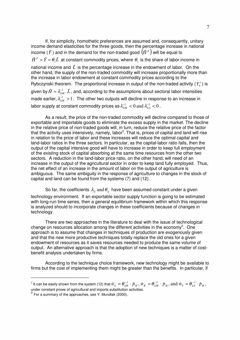
If, for simplicity, homothetic preferences are assumed and, consequently, unitaryincome demand elasticities for the three goods, then the percentage increase in nationalincome ( Y ) and in the demand for the non-traded good ( )dH will be equal to

LYH ld ˆˆˆ θ== at constant commodity prices, where lθ is the share of labor income in

national income and L is the percentage increase in the endowment of labor. On theother hand, the supply of the non-traded commodity will increase proportionally more thanthe increase in labor endowment at constant commodity prices according to theRybczynski theorem. The proportional increase in output of the non-traded activity ( s

hY ) is

given by LH LMˆ .ˆ 1−= λ , and, according to the assumptions about sectoral labor intensities

made earlier, 11 >−LMλ . The other two outputs will decline in response to an increase in

labor supply at constant commodity prices as 0 and 0 11 << −−LALM λλ .

As a result, the price of the non-traded commodity will decline compared to those ofexportable and importable goods to eliminate the excess supply in the market. The declinein the relative price of non-traded goods will, in turn, reduce the relative price of the factorthat the activity uses intensively, namely, labor2. That is, prices of capital and land will risein relation to the price of labor and these increases will reduce the optimal capital andland-labor ratios in the three sectors. In particular, as the capital-labor ratio falls, then theoutput of the capital intensive good will have to increase in order to keep full employmentof the existing stock of capital absorbing at the same time resources from the other twosectors. A reduction in the land-labor price ratio, on the other hand, will need of anincrease in the output of the agricultural sector in order to keep land fully employed. Thus,the net effect of an increase in the amount of labor on the output of agriculture isambiguous. The same ambiguity in the response of agriculture to changes in the stock ofcapital and land can be found from the systems (7) and (12).

So far, the coefficients ijij θλ and have been assumed constant under a given

technology environment. If an exportable sector supply function is going to be estimatedwith long-run time series, then a general equilibrium framework within which this responseis analyzed should to incorporate changes in these coefficients because of changes intechnology.

There are two approaches in the literature to deal with the issue of technologicalchange on resources allocation among the different activities in the economy3. Oneapproach is to assume that changes in techniques of production are exogenously givenand that the new more productive techniques totally replace the old ones for a givenendowment of resources as it saves resources needed to produce the same volume ofoutput. An alternative approach is that the adoption of new techniques is a matter of cost-benefit analysis undertaken by firms.

According to the technique choice framework, new technology might be available tofirms but the cost of implementing them might be greater than the benefits. In particular, if

2 It can be easily shown from the system (12) that HLATHLMKHLHL pwpwpw ˆˆ and ,ˆˆ ,ˆˆ 111 ⋅=⋅=⋅= −−− θθθ ,under constant prices of agricultural and imports substitution activities.3 For a summary of the approaches, see Y. Mundlak (2000).

8

new available techniques are capital-intensive, then these techniques are going to beimplemented by firms if the relative price of capital compared to other factors of productionis low enough to make them profitable to acquire. Otherwise, firms would keep usingtraditional techniques that are less intensive in the use of capital and the new ones wouldnot be adopted. Thus, this approach emphasizes the differences between availabletechnology and implemented production techniques. The rate of adoption of productiontechniques by firms within the envelope of the available technology set would thus be amatter of economic choice and this would depend upon economic incentives that theyface.

Economic incentives to implement new techniques include relative prices and thecapital-labor and land-labor ratios. If there were an increase in the relative price ofexportable agriculture resulting, for instance, from a reduction in import tariffs, and if thiswould result in increases in the prices of labor and land compared to that of capital. As aresult, labor- and land-saving techniques were going to be adopted. If, on the other hand,there were an increase in the overall capital-labor ratio and, as a result, prices of laborcompared to that of capital and land would rise, then firms would find more profitable toadopt techniques that labor-saving.

The available technology set is hard to measure as it is embodied in knowledgeand, thus, in human capital. Schooling and expenditure in research and development canbe measures of the available technology as they represent investment in human capital.Quality of schooling and profitability of research and development are issues that are hardto deal with actual data. Alternatively, as the human capital factor is a complement of theother factors of production, these factors are going to be positively related with knowledge.This analysis suggests specifying a technique choice function (Ti) for firms in sector i as,

= LTK

pp

fTm

xii , , , (15)

The results of this section can be summarized in an aggregate agriculturalsupply function like the following:

LTKpp

Am

x lnlnlnln ln 43210 βββββ +++

+= (16)

where the

’s include not only the direct effect of the variables on agricultural output butalso their impact on the rate of adoption of technology given the available state of the arts.

2. The Results of the Estimation

In this section, the agricultural supply function (16) is estimated with annual datacovering the period 1939-1984 for which data is available4. On the basis of the Phillips-Perron test, the null hypothesis that all the variables of the agricultural supply function arenon stationary cannot be rejected by the data (see Table 1 below). The p-values areobtained from the surface response function estimated by MacKinnon (1993) that permits

4 For a description of the data, see Annex B.

9

the calculation of the Phillips and Perron critical values for any sample size and for anyright-hand variables.

Table 1: Phillips-Perron (PP) Test for Unit Roots

Variables PP statistic p-values

ln(A) -1.31 0.62

ln(px/pm) -0.68 0.42

ln(K) 1.55 0.99

ln(L) -1.25 0.64

ln(T) 0.70 0.99

Notes: With the exception of the logarithm of the relative price of agriculture, all the variables show a trend in their levels and a deterministic constant was thus added tothe first differences of the variables in the PP unit root tests.

Non stationary variables mean that a linear combination of them may be stationaryand this is what has been referred in the literature as cointegration vectors that areinterpreted as long run equilibrium relationships. One method of estimating the long runparameters of the agricultural supply function is that of Johansen and Juselius (1990). Inorder to estimate the number of stationary long run equilibrium equations, a cointegrationtest has to be performed. Consider first the following autoregressive model

tktkttt XXXX ε+Π++Π+Π= −−− ...2211 (t=1,…,T) (17)

where st ´ε are independent Gaussian variables with 0 mean and variance Xt is apx1 vector of stochastic variables.

As most economic time series are non stationary, it is convenient to rewrite themodel (17) as:

tktkttt XXX ε+Π+Γ++∆Γ=∆ −+−− 111 ... (18) L, and L is the lag operator

∑+=

Π−=Γk

ijji

1

, and

Π−−=Π ∑

=

k

ii

1

1

As demonstrated by Johansen and Juselius (1990), testing the number of

cointegration vectors amounts to determine the rank of the matrix . The hypothesis thatthe rank of is r can be formulated as the restriction that where the vector is thecointegrating vector with the property that is stationary, and can be interpreted as theaverage rate of adjustment of the variables towards their long run equilibrium values, and

10

! and " are p x r vectors. If the hypothesis that r=0 is rejected, then the matrix # containsinformation about long-run relationships between the variables in the data.

Johansen (1990, 1991) has developed two test statistics to test the cointegration$&%')(+*-,/.10-2 3 465-7981: ;/<)=54>? @A<B79C->D>: EF>=HG-5?JI->K5=-L679C->67M8N5AOH>QP7N579: P71: OBPARTSUPB@V4QWB7&X71: OYO89: 71: OH5?values for these test statistics are provided by Doornik, J. A. (1998). The asymptoticdistribution of the test statistics depends upon the assumptions about the deterministicterms included in (17).

As demonstrated by Cheung and Lai (1993), the critical asymptotic values of thetwo tests statistics tend to overestimate the number of statistically significant cointegrationvectors in small samples. They also find that the trace test statistic shows little bias in thepresence of either skewness or excess kurtosis and that the maximal eigenvalue testshows substantial bias in the presence of large skewness although it is quite robust toexcess kurtosis.

Cheung and Lai (1993), and Ahn and Reinsel (1990) proposed small samplecorrections based on the degrees of freedom. While Cheung and Lai (1993) correct theasymptotic critical values of the test statistics, Ahn and Reinsel (1990) correct the teststatistics. Cheung and Lai show that the Ahn-Reinsel method does not yield unbiasedestimates of the finite sample critical values for Johansen´s tests. The distribution of thetest statistics in small samples depends not only on the degrees of freedom but also on theparameters of the vector autoregression under the null hypothesis about the number ofcointegrated vectors. Both of the mentioned degrees of freedom corrections capture partof this dependence on the lag length but not the dependence upon the parameters.

Johansen (2002) derives a Bartlett correction factor of the trace test statistic toimprove its finite sample properties. The Bartlett procedure amounts to find theexpectation of the likelihood ratio test and correcting it to have the same mean as the limitdistribution. The correction factor is a function of the estimated values of the parameters( )ΩΓ ˆ and ,ˆ , , iβα under the null hypothesis about the number of cointegration vectors (r)and the deterministic terms, and under the assumption of Gaussian errors. If, for instance,it is assumed that r = 0, then the correction factor will only be a function of ( ) and ˆ ΩΓi . If,on the other hand, r = n, the correction factor is calculated using the estimatesof ( ) and ,ˆ..., ,ˆ , , n1 ΩΓΓβα .

The unrestricted parameters of the vector autoregression (17) are estimated withtwo lags in the levels of the variables based on the likelihood ratio test and the Hannanand Quinn criterion. In small samples, however, the use of the likelihood ratio test wouldlead to spurious rejection of the null hypothesis because the small sample distribution ofthe test statistic differs from its asymptotic distribution. Thus, the likelihood ratio test isadjusted for degrees of freedom to correct the small sample bias of the unadjustedlikelihood ratio. In addition, the White test statistic indicates that the hypothesis ofhomoskedastic disturbances cannot be rejected with a marginal probability of about 20percent.

The test of the null hypothesis of Gaussian residuals is based on the Jarque-Beratest statistic with a correction for small samples as proposed by Doornik and Hansen(1994) for both the individual equations and the system of equations as a whole. The

11

residuals are orthogonalized according to the procedure of Doornik and Hansen (1994)that makes the test statistic invariant with respect to the ordering of the variables (as withthe Choleski orthogonalization. Furthermore, the Doornik and Hansen´s procedureZ9[N\]-^_N`[Mab^Y^cedf]-dA^H^b\]-ghc-i)[jZN`V^Vk ^YZN`D\l/lA[N`m)kJan\Zdo p q 2 in small samples.

For the system as a whole, the null hypothesis of normality cannot be rejected byr9s-tQu/v-r&vQv)wxr9s-tbq 2 (10) test statistic is calculated for the system as a whole in 4.09 with amarginal significance level (the p-value) of 94 percent. The null hypothesis of seriallyuncorrelated residuals is also tested and the Lagrange multiplier test statistic indicates thatit cannot be rejected by the data at one and two lags of the residuals with p-values of 35and 44 percent, respectively. There is no evidence of heteroskedastic disturbancesaccording to the ARCH test5.

In order to calculate the small sample correction factor of the trace statistic underthe null hypothesis of r=0, the model (18) is fitted with one lag of the variables in firstdifferences and a constant in the cointegration space and a linear trend in the data6. Sincethe power of the test is likely to be low against near cointegration alternatives, it seemsreasonable to follow a test procedure that rejects the null hypothesis for higher p-valuesthan the usual 5 percent significance level, say, at 10 percent.

The corrected trace statistic of 72.80 shows that the hypothesis of no cointegrationvector (r=0) is rejected by the data (see table 2 below) with a marginal probability of 2.7percent. The hypothesis of one cointegration vector (r=1) cannot be rejected as thecorrected trace statistic is calculated in 42.93 with a marginal probability of 13.4 percent.

Table 2: Trace Test Statistics for Testing Cointegrating Vectors

r Bartlett CorrectionFactor

TraceStatistic

Corrected TraceStatistic

p- values

0 1.388 101.051 72.802 0.027

1 1.237 53.117 42.931 0.134

Note: The model includes a constant in the cointegration space and a linear trend in the data. The corrected trace statistic is the trace statistic divided by the Bartlett correction factor. The p-

values are approximated using the Γ-distribution, see Doornik (1998).

The estimated cointegration vector (the y 1’s) is as follows (the t-statistics are thenumbers in parenthesis):

ln(A) = 46.055 + 1.256 ln(px/pm) + 2.226 ln(K) + 4.679 ln(T) – 6.701 ln (L) (7.970) (6.466) (4.014) (-7.541)

All the estimated coefficients are significantly different from zero at the usualsignificance levels. In particular, the long-run supply price elasticity is estimated in 1.26and is about three times higher than those estimated by Reca (1980). The estimated 5 See Annex A6 The coefficients to calculate the correction factor have not been tabulated in Johansen, Nielsen, and Fachin(2005). This problem is avoided by using the coefficients of a slightly larger model with a linear trend restrictedto the cointegration space.

12

supply price elasticity is higher than the simulated by Mundlak, Cavallo, and Domenech(1989) with a time horizon of twenty years. The economic interpretation of the coefficientsof the factor endowments is not straightforward because they include not only the effect oftheir changes on agricultural output but also the effects of these changes on relative pricesof non-traded goods. In addition, they may include the impact of these variables on therate of adoption of new technologies.

The average speeds of adjustment of the variables towards their long-runequilibrium states (the α vector) are estimated as follows (the number in parenthesis arethe t-statistics):

Table 4: Estimates of the z vector

ln A ln(px/pm) lnK lnT lnL

-0.114(-3.662)

0.300(4.587)

0.007(1.452)

0.050(3.079)

-0.011(-1.035)

The average speed of adjustment of the agricultural output is -0.11 and thisindicates that convergence to its long-run equilibrium state is achieved in about nine-tenyears. The likelihood ratio test statistic (adjusted by degrees of freedom) under the nullhypothesis that this coefficient is zero is calculated in 4.44 and this hypothesis is rejectedwith a marginal probability of 3.5 percent. In their simulations, Mundlak, Cavallo, andDomenech (1989) implicitly estimate a unit elastic response of agricultural output tochanges in relative prices but the long run equilibrium output is achieved in twenty years7.

Weakly exogeneity tests of the variables can be conducted under the nullhypothesis of αj=0 using the likelihood ratio test adjusted by degrees of freedom that is| ~e11|JAAQ)~+ 2 (1). The value of the test statistic under the null hypothesis that therelative price of agriculture (Px /Pm) is weakly exogenous is 5.14 with a p- value of 2.3percent and this amounts to reject it at the usual significance levels. On the other hand,the test statistic calculated under the null hypothesis that land is weakly exogenous is 4.85and this value amounts to reject it with a p-value of about 2.8 percent. Furthermore, thehypothesis that capital and labor are weakly exogenous cannot be rejected by the data.

The interpretation of causal relationships among variables is not straightforward.For instance, a government policy reaction function can induce causality from output toprices although they are structurally exogenous and simulations based on the estimatedparameters can be subject to the Lucas’ criticism (1981). In the case of the relative pricevariable, a plausible explanation for the lack of weakly exogeneity could be a feedbackpolicy reaction that relates taxation of exports to a booming agricultural economy. Analternative hypothesis is that the international prices of agricultural commodities areaffected by Argentinean agricultural output variations in which case the country would notbe a small economy in international markets. This is certainly an issue that deservesadditional research because if the country is a price maker in world markets, then an

7 See Mundlak, Y., D. Cavallo, and R. Domenech (1989), Table 19, page 96.

13

export tax would maximize welfare from the country’s standpoint in absence of importtaxes.

As mentioned earlier, the hypothesis that land is weakly exogenous is rejected bythe data. One explanation could be that if the error correction vector contains, in additionto its own equilibrium correction process, information about stationary technologicalshocks that are land saving and if these shocks affect the use of land by the variousagricultural crops differently, then this could be reflected in the output weighted cultivatedland and a causal ordering would follow.

Mundlak, Cavallo, and Domenech (1989) include several macroeconomic variablessuch as inflation, deflation, and bank failures in their estimates of agricultural productionfunctions. A model consisting of the six variables including fiscal deficit (d as a percentageof GDP8 is fitted with two lags, and an unrestricted constant term. Fiscal deficits can havenegative effects on sectoral outputs through potential distortions caused by the inflation taxand/or crowding out effects of public sector borrowing over the private sector.

The results of the estimation indicate that the hypothesis of normally distributedresiduals cannot be rejected as the multivariate Jarque-Bera test statistic (χ2(12)) iscalculated in 8.46 with a marginal probability of 75 percent. On the other hand, the LMstatistics to test the hypothesis of uncorrelated residuals are calculated at one and twolags in 34.92 and 33.56, respectively, and these values indicate that the null hypothesiscannot be rejected. On the other hand, the hypothesis of homoskedastic disturbances isnot rejected by the data as the multivariate ARCH test statistics are calculated in 454.0and 924.0 for one and two lags, respectively with marginal probabilities of 32 and 16percent.

The cointegration rank of the cointegrating model is determined by comparing thetrace statistic adjusted by the Bartlett small sample correction factor with the asymptoticcritical values at 10 percent significance level. The results indicate (see table 3) that thehypothesis of r= 1 cannot be rejected at this significance level.

Table 3: Trace Test Statistics for Testing Cointegrating Vectors

r Bartlett CorrectionFactor

TraceStatistic

Corrected TraceStatistic

p-values

0 1.4137 129.889 91.173 0.098

1 1.2790 77.805 60.832 0.211

Note: See Table 2.

The estimated cointegrating vector is as follows:

ln(A) = 33.224 + 1.055 ln(px/pm) + 2.578 ln(K) + 3.137 ln(T) – 6.547 ln(L) – 0.023 ln(d) (7.810) (6.433) (2.925) (-7.873) (-2.478)

8 The null hypothesis that the fiscal deficit follows a unit root autoregressive process with a linear trend in thelevel of the variable cannot be rejected by the data as the PP test statistic is calculated in -2.63 and thisamounts not to reject the null with a marginal probability of 9.5 percent.

14

The supply price elasticity is estimated in about 1.0 and this estimate is close tothat of the supply price function that excludes the fiscal deficit. This estimated supply priceelasticity is similar to that estimated in Mundlak, Cavallo, and Domenech (1989) for a timehorizon of twenty years. As expected, the coefficient of the fiscal deficit is negative andstatistically different from zero. The remaining coefficients are all statistically different fromzero and they are quite robust to the inclusion of the fiscal deficit variable.

The speed of convergence of agricultural output towards the long-run equilibrium isestimated in -0.134 and is statistically different from zero. This is another piece ofevidence supporting the existence of one cointegration vector. The hypothesis thatrelative prices and land are weakly exogenous are rejected by the data as the likelihoodratio tests statistics are calculated in 6.6 and 4.1, respectively with marginal probabilities of1.0 and 4.2 percent.

In his aforementioned study, L. G. Reca (1980) includes a dummy variable thattakes a value of zero for the years 1950-1964 and one afterwards to define two differenttechnological levels. According to Reca’s estimates, technological change wasresponsible for an increase in agricultural production of about 8-10 percent between1965and 1974. As the coefficients of the supply function estimated in this paper includes theeffect of prices changes on the adoption of new production techniques, the existence oftwo technological levels before and after 1964 could affect the stability of the parametersover time.

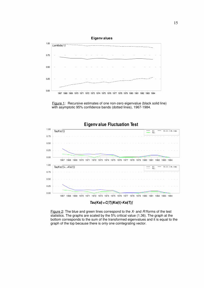
Hansen and Johansen (1999) suggest a graphical procedure to evaluate theconstancy of the long-run parameters over time in cointegrated vector autoregressivemodels. The procedure is based on recursively estimated non-zero eigenvalues as theseprovide information about the adjustment coefficients and the cointegrated vectors andnon-constancy of these parameters will be reflected in the time path of the estimatedeigenvalues. The time paths of the estimated eigenvalues for the sub sample 1967-1984are used as a diagnosis tool in the model evaluation. The size of the sub sample hasbeen chosen as a function of the parameters of the model9. The results are presented inFigure 1 and, although it is not a formal test of stability of parameters, they do not seem toindicate non-constancy of the parameters.

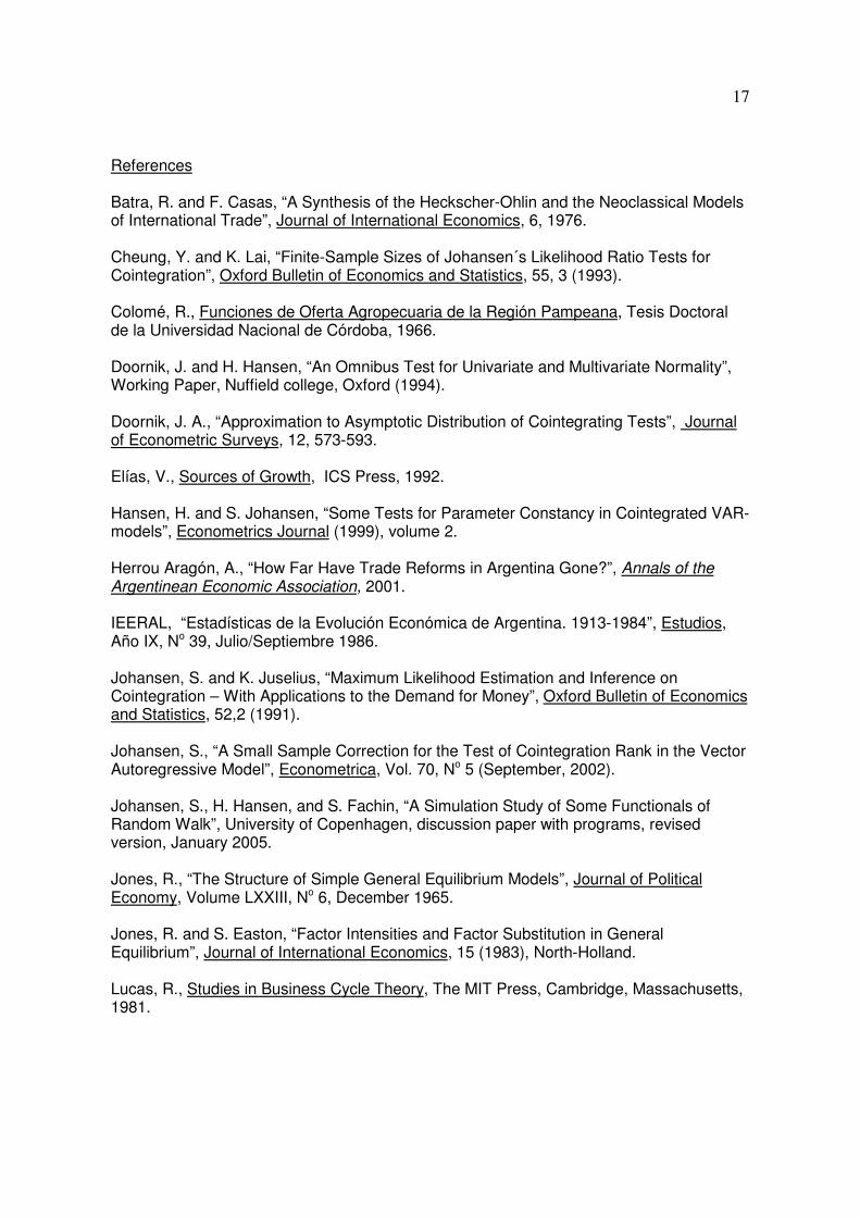
A formal test of stability of parameters over time developed by Hansen andJohansen (1999) is presented in Figure 2, where the fluctuation test of the transformed

eigenvalues is presented. The eigenvalues, λI , are transformed into

−

=i

ii λ

λε

1log to

obtain a better approximation of their limiting distribution. In the recursive analysis, thetest statistics are calculated either by reestimating recursively all the parameters (the so-called X-form), or by reestimating only the long-run parameters α and and concentratingout the short term coefficients (the R1-form). It can be seen that the values of the teststatistics are below the 5% critical level and, consequently, the hypothesis of constancy ofparameters cannot be rejected.

9 In the six variable system including the fiscal deficit, the sub sample to calculate the recursive eigenvaluesincludes the period of time from 1975 until 1984 and, thus, the estimates of the coefficients with the base datacould be affected by the technological innovations of the mid-sixties and, consequently, the stability tests mightnot be reliable For this reason, the eigenvalues of the six variable system have not been recursivelyestimated.

15

Eigenv alues

1967 1968 1969 1970 1971 1972 1973 1974 1975 1976 1977 1978 1979 1980 1981 1982 1983 19840.00

0.25

0.50

0.75

1.00Lambda(1)

Figure 1: Recursive estimates of one non-zero eigenvalue (black solid line) with asymptotic 95% confidence bands (dotted lines), 1967-1984.

Eigenv alue Fluctuation Test

Tau(Ksi) = C(T)||Ksi(t)-Ksi(T)||

1967 1968 1969 1970 1971 1972 1973 1974 1975 1976 1977 1978 1979 1980 1981 1982 1983 19840.00

0.25

0.50

0.75

1.00X( t )R1(t )

5% C. V. (1. 36 = I ndex)Tau(Ksi(1))

1967 1968 1969 1970 1971 1972 1973 1974 1975 1976 1977 1978 1979 1980 1981 1982 1983 19840.00

0.25

0.50

0.75

1.00X( t )R1(t )

5% C. V. (1. 36 = I ndex)Tau(Ksi(1)+...+Ksi(1))

Figure 2: The blue and green lines correspond to the X- and R1forms of the test statistics. The graphs are scaled by the 5% critical value (1.36). The graph at the bottom corresponds to the sum of the transformed eigenvalues and it is equal to thegraph of the top because there is only one cointegrating vector.

16

3. Concluding Remarks

This paper estimates a reduced-form agricultural supply function within theframework of a general equilibrium model. The supply function includes not only sectoralrelative prices but also the stock of factors of production. The response of agriculturaloutput to changes in factor endowments reflect not only changes in the transformationsurface of the economy caused by these changes but also the movement along it resultingfrom the induced changes in relative factor prices. The model is also estimated with theinclusion of a fiscal deficit variable to incorporate the effects of macroeconomic policies onagricultural output.

Technological change is regarded as a variable subject to economic choice byfirms given the available technology and, hence, it is endogenous. Variables that affectthis choice of techniques include relative sectoral prices and factor endowments. Inaddition, the endowment of physical capital (and, perhaps, land) is regarded as a carrier ofthe available technology as it is correlated with human capital and, hence, with knowledge.

The results of the estimations show that there is a statistically significant supplyprice elasticity of the agricultural output in the range of 1.0-1.25 and that the convergenceto the equilibrium state is achieved in a range of about eight to ten years, depending uponthe model estimated. The estimated supply price response is much higher than previousestimates of partial equilibrium models by Reca (1969, 1980), and Colome (1966). Thespeed of convergence is much shorter than that estimated by Mundlak, Cavallo, andDomenech (1989) of about twenty years for a unitary response of agricultural output tochanges in prices. It is also found that fiscal deficits have a statistically significant negativeeffect on agricultural output.

The results also show that, according to the time path of one non-zero eigenvalue,there is no indication of non-constancy of parameters for the period covering 1967-1984,years during which new techniques of production were adopted. A formal fluctuation testof the transformed eigenvalues also indicates that the null hypothesis of constancy ofparameters cannot be rejected by the data.

17

References

Batra, R. and F. Casas, “A Synthesis of the Heckscher-Ohlin and the Neoclassical Modelsof International Trade”, Journal of International Economics, 6, 1976.

Cheung, Y. and K. Lai, “Finite-Sample Sizes of Johansen´s Likelihood Ratio Tests forCointegration”, Oxford Bulletin of Economics and Statistics, 55, 3 (1993).

Colomé, R., Funciones de Oferta Agropecuaria de la Región Pampeana, Tesis Doctoralde la Universidad Nacional de Córdoba, 1966.

Doornik, J. and H. Hansen, “An Omnibus Test for Univariate and Multivariate Normality”,Working Paper, Nuffield college, Oxford (1994).

Doornik, J. A., “Approximation to Asymptotic Distribution of Cointegrating Tests”, Journalof Econometric Surveys, 12, 573-593.

Elías, V., Sources of Growth, ICS Press, 1992.

Hansen, H. and S. Johansen, “Some Tests for Parameter Constancy in Cointegrated VAR-models”, Econometrics Journal (1999), volume 2.

Herrou Aragón, A., “How Far Have Trade Reforms in Argentina Gone?”, Annals of theArgentinean Economic Association, 2001.

IEERAL, “Estadísticas de la Evolución Económica de Argentina. 1913-1984”, Estudios,Año IX, No 39, Julio/Septiembre 1986.

Johansen, S. and K. Juselius, “Maximum Likelihood Estimation and Inference onCointegration – With Applications to the Demand for Money”, Oxford Bulletin of Economicsand Statistics, 52,2 (1991).

Johansen, S., “A Small Sample Correction for the Test of Cointegration Rank in the VectorAutoregressive Model”, Econometrica, Vol. 70, No 5 (September, 2002).

Johansen, S., H. Hansen, and S. Fachin, “A Simulation Study of Some Functionals ofRandom Walk”, University of Copenhagen, discussion paper with programs, revisedversion, January 2005.

Jones, R., “The Structure of Simple General Equilibrium Models”, Journal of PoliticalEconomy, Volume LXXIII, No 6, December 1965.

Jones, R. and S. Easton, “Factor Intensities and Factor Substitution in GeneralEquilibrium”, Journal of International Economics, 15 (1983), North-Holland.

Lucas, R., Studies in Business Cycle Theory, The MIT Press, Cambridge, Massachusetts,1981.

18

MacKinnon, J. G., “Critical Values for Cointegration Tests” in R. F. Engle and C. W.Granger (eds.), Long-run Economic Relationships: Readings in Cointegration, OxfordUniversity press, 1991.

Maddala, G. S., Introduction to Econometrics, Third Edition, Wiley, 2000.

Mundlak, Y., D. Cavallo, and R. Domenech, Agriculture and Economic Growth inArgentina, 1913-1984. Research Report 76, IFPRI, November 1989.

Mundlak, Y., Agriculture and Economic Growth: Theory and Measurement, HarvardUniversity Press, 2000.

Reca, L.G., “Determinantes de la Oferta Agropecuaria en la Argentina 1934/35-1966/67”,Estudios sobre la Economía Argentina, Agosto 1969, Buenos Aires.

- Argentina: Country Case Study of Agricultural Prices and Subsidies, WorldBank Staff Working Paper No 386, April 1980.

Reinsel, G. and S. Ahn, “Asymptotic Properties of the Likelihood Ratio Tests forCointegration in the Nonstationary Vector AR Model”, Technical Report, Department ofStatistics, University of Winsconsin, Madison, 1988.

Rivera-Batiz, F., “Non traded Goods and the Pure Theory of International Trade with EqualNumbers of Goods and Factors”, International Economic Review, Vol. 23, No 2, June1982.

Rodriguez, C., “Salarios Reales y Protección”, Cuadernos de Economía, No 54-55, 1981.

Sjaastad, L., “Commercial Policy, ‘True tariffs’, and Relative Prices”, in John Black andBrian Hindley (eds.), Current Issues in Commercial Policy and Diplomacy, London,MacMillan, 1980.

19

Annex A: Univariate Tests of Residuals

Normality test – Doornik-Hansen procedure:

Equation J-B Test Statistic p-value

lnA 0.331 0.848

ln(Px/Pm) 3.193 0.203

lnK 0.203 0.903

lnT 2.609 0.271

lnL 0.745 0.689

ARCH test of heteroskedasticity:

Equation ARCH(2) p-value

lnA 0.038 0.981

ln(Px/Pm) 0.149 0.928

lnK 1.068 0.586

lnT 2.963 0.227

lnL 0.113 0.945

Normality test – Doornik-Hansen procedure:

Equation J-B Test Statistic p-value

lnA 0.602 0.740

ln(Px/Pm) 0.616 0.735

lnK 0.079 0.961

lnT 1.350 0.509

lnL 1.320 0.517

d 4.034 0.133

ARCH test of heteroskedasticity:

20

Equation ARCH(2) p-value

lnA 1.403 0.496

ln(Px/Pm) 0.366 0.833

lnK 1.966 0.374

lnT 1.457 0.483

lnL 1.460 0.482

d 0.159 0.924

21

Annex B: Data Description

A: Agricultural output at 1960 prices. Source: IERRAL, op. cit.(Px/Pm) : Price of agricultural goods divided by the price of imported goods. Source:from 1939 until 1965, Diaz-Alejandro, C. F., Ensayos sobre la Historia EconómicaArgentina, Amorrortu editores. From 1966 until 1984: INDEC.K : Stock of capital employed in production of goods and services in australes at 1960prices. Source: IEERAL, op. cit.T : Total planted area in thousand of hectares weighted by the value of production ofeach crop. Source: IEERAL, op. cit.L: Total labor force in million people. Source IEERAL, op. cit.D: Consolidated fiscal deficit as percentage of the gross domestic product at currentprices. Source: IERAL, op. cit.