1

Agricultural Risk, Insurance, and the

Land-Productivity Inverse Relationship Huang Chen

University of California, Davis

Abstract:

China is attempting to improve upon existing land entitling policy to stimulate rural

land aggregation trend for absorbing rural labors to support urban development.

However, the potential negative impact of land size increase on farm productivity, i.e.

the Inverse Relationship (IR), is triggering an intensive debate. Given the fact that

China’s agricultural insurance market has grown rapidly in recent years, the purpose

of this study is to investigate whether the insurance boosts large farms’ productivity

more than smaller farms’, so that the establishment of an insurance market can

complement the development of land markets, and mitigate the concern of IR. To

answer this question, the first part of this study analyzes the role of risk in affecting

productivity. A general farm profit model is developed and the result brings an

additional layer to the conventional conclusion in literature about the risk and the IR:

a constant relative risk averse (CRRA) farmer still suffers from IR problem. The

second part of the model shows that insurance can indeed boost productivity, and the

impact of the insurance for large farms is bigger than the small farms. In the last

theory section, three explanations of IR are decomposed and compared to see how

their different roles in affecting productivity. The theoretical findings are

econometrically tested using a large-scale filed survey data from 6 provinces in

northern China. Insurance policy is employed as IV for dealing with the endogeneity

of farmers' insurance purchase behavior. Results show that insurance can significantly

boost productivity by 25%, and substantially mitigate the IR. Policy implications for

land and insurance market developments are discussed.

Key Words: Risk, Insurance, Land-Productivity Inverse Relationship, IV

2

1. Introduction

The Chinese government has consistently been trying to relocate agricultural labors

from rural area to urban area for supporting industrial development (Meng, 2012),

especially after the increase of urban labor cost was criticized as a main source of the

slowdown of its rapid GDP growth rate in recent years (CPG, 2013, 2014; Eggleston

et al., 2013; Li et al., 2012). Among the package of policies released to encourage

migration, land (use-right) entitlement is widely considered a fundamental policy that

secures the development of rural land rental markets, resulting in a promised

emergence of land aggregation trends and the increase of farmers’ non-farm works

(Deininger et al., 2014; Kung, 2002; NDRC, 2009).

However, there is growing concern on the potential negative impacts of the land

aggregation trend on agricultural productivity, given that the land-productivity inverse

relationship (IR) has commonly been found in the literature (Fan and Chan‐Kang,

2005; Jin and Deininger, 2009). Rada (2015) finds direct evidence showing that grain

yields likely will decline as current farm-scale expansion progresses. Wang (2016)

and Deininger (2014) also confirm the existence of the IR in China using different

data sets. To ensure food security in the world’s most populous country, a stream of

new subsidies and incentive programs to support farm production have been

implemented (MOA, 2013, 2014).

3

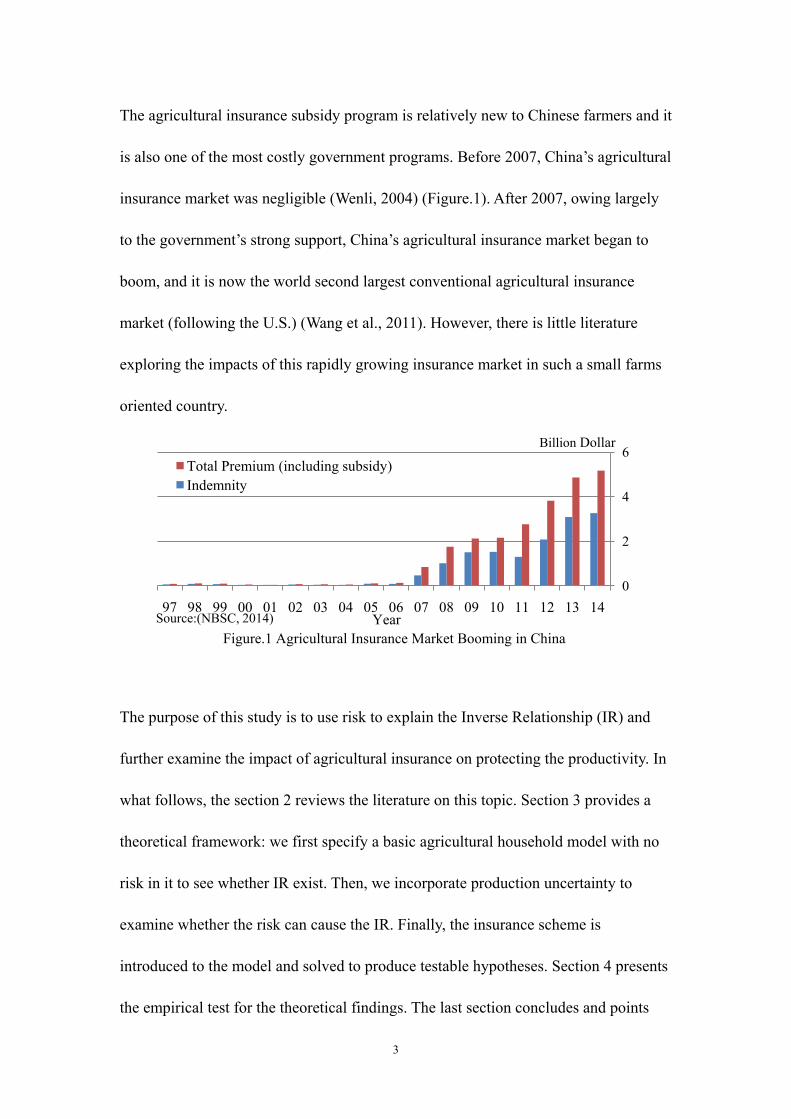
The agricultural insurance subsidy program is relatively new to Chinese farmers and it

is also one of the most costly government programs. Before 2007, China’s agricultural

insurance market was negligible (Wenli, 2004) (Figure.1). After 2007, owing largely

to the government’s strong support, China’s agricultural insurance market began to

boom, and it is now the world second largest conventional agricultural insurance

market (following the U.S.) (Wang et al., 2011). However, there is little literature

exploring the impacts of this rapidly growing insurance market in such a small farms

oriented country.

The purpose of this study is to use risk to explain the Inverse Relationship (IR) and

further examine the impact of agricultural insurance on protecting the productivity. In

what follows, the section 2 reviews the literature on this topic. Section 3 provides a

theoretical framework: we first specify a basic agricultural household model with no

risk in it to see whether IR exist. Then, we incorporate production uncertainty to

examine whether the risk can cause the IR. Finally, the insurance scheme is

introduced to the model and solved to produce testable hypotheses. Section 4 presents

the empirical test for the theoretical findings. The last section concludes and points

0

2

4

6

141312111009080706050403020100999897

Billion Dollar

YearFigure.1 Agricultural Insurance Market Booming in China

Total Premium (including subsidy)Indemnity

Source:(NBSC, 2014)

4

out the policy implication from this study.

2. Literature Review

Literature has pointed out there are many potential candidates for explaining the IR

phenomenon, such as imperfect labor market (Mazumdar, 1965; Sen, 1962), existence

of supervision cost on hired labors (Feder, 1985), scale economies (Townsend et al.,

1998), land quality (Benjamin, 1995; Bhalla and Roy, 1988), and even

methodological shortcomings in studying this topic (sample selection bias based on

illiteracy, ignorance of village effect in econometric approach, and measurement error

on farm size) (Carletto et al., 2013; Carter, 1984). It’s important to note that,

sometimes, we may not be able to observe the IR in our data, as yields are

endogenously determined through changes in technology and mechanization (Bardhan,

1973; Gorton and Davidova, 2004; Sheng et al., 2015). Whether the IR can be

observed in field works depends on the particular external circumstances of the region

under study.

Only a handful of papers in the literature point out that risk can be another candidate

for explaining the IR.1 Three papers point out that production risk can be a reason for

explaining IR, but two of them specifically require farmers to be increasing relative

risk averse (IRRA) to obtain IR result (Feder,1980; Just and Zilberman, 1983).

1 Surprisingly, they are all among the most cited papers in the research filed of explaining the IR According to Google Scholar search, there are approximately 100 papers focusing on the IR with more than 10 citations by July 10, 2016. Only five papers use risk to explain the IR. One of them has more than 1000 citations, three of them have approximately 300 citations, and the least one has 73 citations.

5

Srinivasan (1972) shows a boarder conclusion that non-decreasing RRA can lead to

IR, but such a finding strictly relies on an assumption on the two technologies

specified in the paper. Moreover, actually, all of the three papers model the farmers

have two types of risky technologies to choose when making planting decision. This

study is going to show that there is a more general and straightforward conclusion

between production risk and IR, not relying on the IRRA assumption on farmers' risk

altitude or complicated production technologies. Even farmers are constant relative

risk averse (CRRA) and only one technology is available for them, the IR still exists.

It is worth to mention that Rosenzweig and Binswanger (1993) and Barrett (1996)

study risk and the IR from different points of views. The former study assumes

large/wealth farmers have better income smoothing ability than small/poor farmers,

giving the large/wealth farmers more risk tolerance, therefore, their expected

productivity is higher than small/poor farmers. In other words, Rosenzweig and

Binswanger (1993) disagree with the argument that risk causes the IR. But whether

large farmers in developing countries have better financial situation than small

farmers is questionable. For example, nonfarm departments China are relatively well

developed, and small farmers usually have substantial higher non-farm incomes than

large farmers. Another thing worth noting is that the large farmers are new emerged

ones, they may not have accumulated enough wealth to provide buffers for

agricultural shock. The latter study (Barrett, 1996) uses price uncertainty to explain

why small farms tend to over invest in crops, while the large ones tend to under invest.

6

Since small farms are more likely to be net buyers and large farms are more likely to

be net sellers in product markets, the price uncertainty generates a positive and

negative risk premium for the small and large farms’ own productions, respectively,

resulting in different input intensity levels.

3. Theoretical Model

3.1 Model Introduction

In this study, we focus on production uncertainty. Three possible explanations for IR

will be considered. Except the risk, the other two explanations are the agency cost and

the property of return to scale of agricultural technology. Although we include these

two explanations in our model setting, for focusing on the role of risk, the results

presented here are assuming there is not agency cost and the technology is constant

return to scale (CRS), except in the end of this section, we reassume the two factors

exist in order to decompose the effects of the three explanations for comparing their

different contribution to IR and figuring out is there joint effect of different

explanations. Farmers will be assumed to be constant relative risk averse, CRRA, for

eliminating the impact of relative risk preference.

Based on the degree of complexity, the modeling process is divided into three phases:

Phase-1: Basic Model, in which there is no risk, illustrates the basic relationship

between land, labor endowments and farmer productivity. Phase-2: Risk Model

includes uncertainty in the production function, so that the effect of risk can be found.

7

Phase-3: Insurance Model assumes farmers can buy insurance against risk, so the

results can be used to answer a practically meaningful question whether insurance can

recover the lost productivity due to risk avoiding action, and mitigate the IR.

3.2 Basic Model

3.2.1 Model Setting

Total Farm Income (𝛱𝛱):

𝛱𝛱 = 𝜋𝜋 + 𝑁𝑁 = (𝑌𝑌 − 𝐶𝐶) + 𝑁𝑁

where 𝛱𝛱 is total farm income, 𝜋𝜋 is farm (net) income, 𝑁𝑁 is non-farm income, 𝑌𝑌 is

total farm output value (price of output is normalized to be 1), and 𝐶𝐶 is total farm

cost.

Farm Product (𝑌𝑌):

Modern agricultural production should at least have three types of inputs: labor, land,

and intermediate material inputs (seeds, fertilizers, pesticides, irrigation water, et al.).

However, for focusing on the effect of land scale and labor, we use a simplified

production function by assuming that the intermediate material inputs per area is fixed,

i.e. we are imposing a Fixed-Input Assumption for this study. The production function

is denoted as 𝑔𝑔(. ), assuming it has a Cobb-Douglas function form, and 𝑔𝑔𝑖𝑖′ > 0,

𝑔𝑔𝑖𝑖𝑖𝑖′′ < 0, 𝑔𝑔𝑖𝑖𝑖𝑖′′ > 0, 𝑖𝑖 and 𝑖𝑖 = 1 and 2:

𝑔𝑔(𝐸𝐸,𝑇𝑇) ≡ 𝛼𝛼𝐸𝐸𝛽𝛽𝑇𝑇𝛾𝛾

where 𝐸𝐸 is the Effective Labor Input, 𝑇𝑇 is the land input, 𝛽𝛽 is the output elasticity

8

of effective labor; 𝛾𝛾 is the generalized output elasticity of land; and 𝑎𝑎 is the

generalized total factor productivity (TFP).2 We capture the property of return to scale

by simply assigning 𝛽𝛽 + 𝛾𝛾 = (< 𝑜𝑜𝑜𝑜 >)1 for constant (decreasing or increasing)

return to scale technology assumption.

Effective Labor Input (𝐸𝐸):

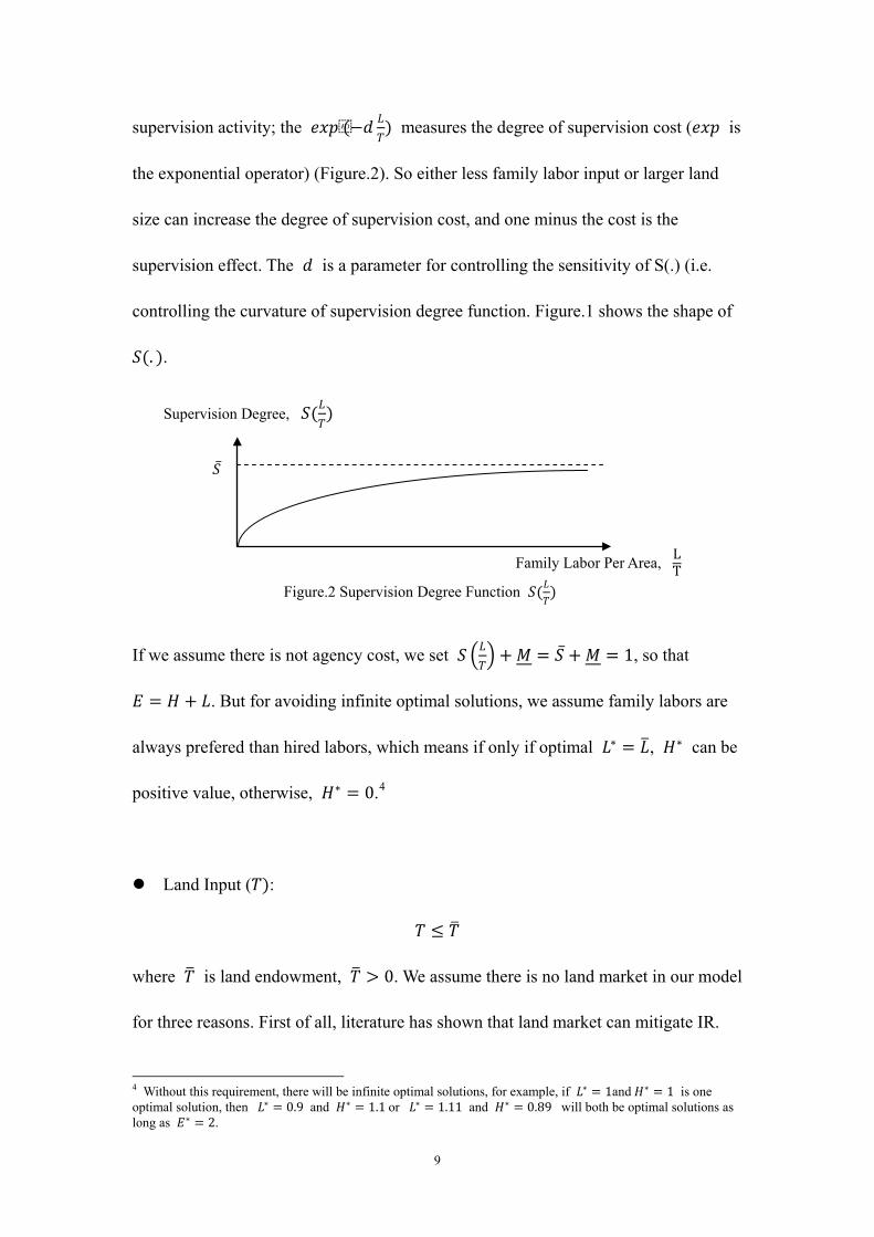
𝐸𝐸 = 𝐻𝐻 ∗ [𝑆𝑆 �𝐿𝐿𝑇𝑇�

+ 𝑀𝑀 ] + 𝐿𝐿

where 𝐻𝐻 is the number of hired labors; 𝐿𝐿 is the family labors, and denote 𝐿𝐿� as

family labor endowment, 𝐿𝐿� > 0. To capture the effect of agency cost in our model,

assume the contribution of hired labors on effective labor input need to be discounted

by multiplying an agency cost multiplier, [𝑆𝑆 �𝐿𝐿𝑇𝑇� + 𝑀𝑀], where 𝑆𝑆(. ) measures

supervision degree imposed by family labors on hired labors, and 𝑀𝑀 > 0 is the

minimum degree of effort that hired labors will guarantee when there is no

supervision activity, driven by their moral standard.3 Assume 𝑆𝑆′ ≥ 0, 𝑆𝑆′′ ≤ 0, which

means as family labor per area increases, hired labors will work harder, but this

supervision effect marginally decreases. Moreover, we explicitly assume:

𝑆𝑆 �𝐿𝐿𝑇𝑇�

= 𝑆𝑆̅ ∗ �1 − 𝑒𝑒𝑒𝑒𝑒𝑒(−𝑑𝑑𝐿𝐿𝑇𝑇

)�

where 𝑆𝑆̅ > 0 is the maximum degree of effort of a hired labor that can be affected by

2 More details of transforming a production function with three inputs to a production function with two inputs using the Fixed-Input Assumption and the meaning of the word “generalized” in describing 𝑎𝑎 and 𝛾𝛾 can be found in Appendix.I. 3 The reason to add moral standard constraint, 𝑀𝑀, is that when land size goes very large, supervision cost becomes extremely high, and 𝑆𝑆(𝐿𝐿

𝑇𝑇) is too close to zero, resulting no one want to hire labors. But, in real world,

large farms still hire labors. There must be something driving the hired labors to work effectively even there is almost not family labor to supervise them all the time. I assume it is the moral standard or the “spirit of agreement” in the society playing the role to ensure hired labors to work at some least levels.

9

supervision activity; the 𝑒𝑒𝑒𝑒𝑒𝑒(−𝑑𝑑 𝐿𝐿𝑇𝑇

) measures the degree of supervision cost (𝑒𝑒𝑒𝑒𝑒𝑒 is

the exponential operator) (Figure.2). So either less family labor input or larger land

size can increase the degree of supervision cost, and one minus the cost is the

supervision effect. The 𝑑𝑑 is a parameter for controlling the sensitivity of S(.) (i.e.

controlling the curvature of supervision degree function. Figure.1 shows the shape of

𝑆𝑆(. ).

If we assume there is not agency cost, we set 𝑆𝑆 �𝐿𝐿𝑇𝑇� + 𝑀𝑀 = 𝑆𝑆̅ + 𝑀𝑀 = 1, so that

𝐸𝐸 = 𝐻𝐻 + 𝐿𝐿. But for avoiding infinite optimal solutions, we assume family labors are

always prefered than hired labors, which means if only if optimal 𝐿𝐿∗ = 𝐿𝐿�, 𝐻𝐻∗ can be

positive value, otherwise, 𝐻𝐻∗ = 0.4

Land Input (𝑇𝑇):

𝑇𝑇 ≤ 𝑇𝑇�

where 𝑇𝑇� is land endowment, 𝑇𝑇� > 0. We assume there is no land market in our model

for three reasons. First of all, literature has shown that land market can mitigate IR.

4 Without this requirement, there will be infinite optimal solutions, for example, if 𝐿𝐿∗ = 1and 𝐻𝐻∗ = 1 is one optimal solution, then 𝐿𝐿∗ = 0.9 and 𝐻𝐻∗ = 1.1 or 𝐿𝐿∗ = 1.11 and 𝐻𝐻∗ = 0.89 will both be optimal solutions as long as 𝐸𝐸∗ = 2.

𝑆𝑆̅

Supervision Degree, 𝑆𝑆(𝐿𝐿𝑇𝑇

)

Family Labor Per Area, LT Figure.2 Supervision Degree Function 𝑆𝑆(𝐿𝐿

𝑇𝑇)

10

For find other explanations rather than just missing land market, we shut down land

market in our model. Secondly, the land markets in developing countries are not well

developed in most of cases; even in developed countries, land as an production asset

cannot be easily traded due to transaction cost, information unavailability, and

geographic inaccessibility. Lastly, land contracts usually last more than one year, so

farmers cannot arbitrarily change the land size in one growing season. More

accurately speaking, we assume our model is a short-run model, i.e. single production

period model, so land endowment is fixed.

Total Farming Cost (𝐶𝐶):

𝐶𝐶 = 𝑊𝑊 𝐻𝐻 + 𝐶𝐶𝑒𝑒𝑇𝑇

where 𝑊𝑊 is the wage of hired labors, 𝐶𝐶𝑒𝑒 is the cost of the fixed inputs per unit land.

As we discussed before, for simplicity, we assume intermediate material input is fixed.

But, in real world, this fixed input cost can be a very small number, such as just

seeding cost and harvesting cost.

Non-Farm Income (𝑁𝑁):

𝑁𝑁 = 𝑊𝑊𝐿𝐿𝑁𝑁 = 𝑊𝑊(𝐿𝐿� − 𝐿𝐿)

where 𝐿𝐿𝑁𝑁 is farm household's non-farm works, so 𝐿𝐿� = 𝐿𝐿𝑁𝑁 + 𝐿𝐿. One implicit but

important assumption here is that the labor hiring department has not risk, so cash

flow from doing nonfarm or hiring workers is risk free.

11

3.2.2 Profit Maximization Problem of Basic Model

Since in the Basic Model, there is no risk, the farmer’s utility can be directly

optimized by maximizing the total farm income 𝛱𝛱. The farmer’s profit maximization

problem (PMP) is:

𝑚𝑚𝑎𝑎𝑒𝑒𝐿𝐿,𝐻𝐻,𝑇𝑇

𝛱𝛱 = 𝑌𝑌 − 𝐶𝐶 + 𝑁𝑁

= 𝛼𝛼𝐸𝐸𝛽𝛽𝑇𝑇𝛾𝛾 − (𝑊𝑊 𝐻𝐻 + 𝐶𝐶𝑒𝑒𝑇𝑇) + 𝑊𝑊(𝐿𝐿� − 𝐿𝐿)

𝑠𝑠. 𝑡𝑡. 𝐿𝐿 ≤ 𝐿𝐿� … 𝜌𝜌1

𝑇𝑇 ≤ 𝑇𝑇� … 𝜌𝜌2

𝐿𝐿 ≥ 0 … 𝜌𝜌3

𝑇𝑇 ≥ 0 … 𝜌𝜌4

𝐻𝐻 ≥ 0 … 𝜌𝜌5

𝐻𝐻(𝐿𝐿� − 𝐿𝐿) = 0 … 𝜌𝜌6

where 𝐸𝐸 = 𝐻𝐻[𝑆𝑆̅ �1 − 𝑒𝑒𝑒𝑒𝑒𝑒(−𝑑𝑑 𝐿𝐿𝑇𝑇

)� + 𝑀𝑀 ] + 𝐿𝐿 if we assume there is agency cost,

otherwise, 𝐸𝐸 = 𝐻𝐻 + 𝐿𝐿. Denote 𝜌𝜌𝑖𝑖 , 𝑖𝑖 = 1,2, … ,6 as the Lagrange Multipliers for the

corresponding constraints. The mathematical process of solving the PMP can be found

in Appendix.II.

Since our primal interesting is in the role of risk, for the Basic Model, we briefly

discuss the result without agency cost assumption in Figure.3, which depicts four

patterns of optimal solutions (marked by the arrows) in four regions of the land and

labor endowment space. First of all, the four regions are divided by three endowment

thresholds (𝑇𝑇�𝜌𝜌1=0,𝜌𝜌2=0, 𝐿𝐿�𝜌𝜌1=0,𝜌𝜌2=0, and 𝐿𝐿�𝜌𝜌1=0,𝜌𝜌2>0) and the solid line displays the

final optimal solutions.5 Region A and B represent the farmer has too many labor

5 The formulas of the cutoffs will be in the Appendix.II, which will be updated in next version....

12

endowment, so the farmer will do some nonfarm works, making sure 𝐿𝐿∗ =

𝐿𝐿�𝜌𝜌1=0,𝜌𝜌2=0 < 𝐿𝐿� in Region A or 𝐿𝐿∗ = 𝐿𝐿�𝜌𝜌1=0,𝜌𝜌2>0 < 𝐿𝐿� in Region B, i.e. arrows

pointing down means selling labors, and the distances measure the number of

nonfarm works. In contrast, Region C and D show that when the farmer has limited

labor endowment, he/she will hire labors to do farm works, i.e. arrows point up and

the distances measure the size of 𝐻𝐻∗. Between the dash threshold line 𝑇𝑇�𝜌𝜌1=0,𝜌𝜌2=0,

Region A and D means the farmer has too large land endowment. Since we assume

there is fixed cost for cultivating land, so optimal choice is to left some of lands

uncultivated. In Region B and C, the farmer has not enough lands, so he/she will

cultivate all of available lands, therefore the arrows in Region B and C are strictly

vertical, i.e. 𝑇𝑇∗ = 𝑇𝑇� < 𝑇𝑇�𝜌𝜌1=0,𝜌𝜌2=0.

Note that, if we assume the technology is CRS, then, the Region A and D disappear,

since 𝑇𝑇�𝜌𝜌1=0,𝜌𝜌2=0 = ∞ and 𝐿𝐿�𝜌𝜌1=0,𝜌𝜌2=0 = ∞ (formulas in Appendix.II), and in Region

B and C no IR will be found, so productivity is constant cross all of endowment

B

A

D C

𝐿𝐿�

𝑇𝑇�

𝐿𝐿�𝜌𝜌1=0,𝜌𝜌2=0

𝐿𝐿�𝜌𝜌1=0,𝜌𝜌2>0

𝑇𝑇�𝜌𝜌1=0,𝜌𝜌2=0

No IR Found

No IR Found

IR Found if Tech. is DRS No IR Found if Tech. is CRS

0 Figure.3 Four Regions of the Optimal Choice Pattern

IR Found if Tech. is DRS No IR Found if Tech. is CRS

Sell Labors

Hire Labors Waste Lands

Hire Labors

13

combinantions.

3.2.3 Numerical Simulation of Basic Model

Though the Basic Model is still mathematically traceable, after introducing risk, the

model becomes unsolveable, we have to rely on numberical simulation to see the

effect of risk and insurance. For comparing with the risk and insurance results, we

first run simulation on the Basic Model. Different calibration in this study will change

the scale of results presented, but will not fundamentally change the conclusion.

Here is how the simulation is calibrated: first of all, the social parameters are

calibrated according to survey data in 6 provinces in the north China: price of output

is 1 Yuan/Jin, non-farm wage 𝑊𝑊 = 120 Yuan/Man-Day, and input cost per mu

𝐶𝐶𝑒𝑒 = 500 Yuan/Mu. Secondly, the technology parameters: 𝛼𝛼 = 700 is set by

gurranting the yield level (after introcing risk) is arround survey data level. Output

elasticities are arbitrily calibrated. Assume 𝛽𝛽 = 0.5 and 𝛾𝛾 = 0.5 for CRS technology,

i.e. 𝛽𝛽 + 𝛾𝛾 = 1. Lastly, the land size is allowed to vary between 0 to 220 Mu, and the

labor endowment is allowed to vary between 0 man-day to 1000 Man-Days. Figure.3

shows the result, in which we find that the productivity does not change, i.e. no IR

found.6

6 Small fluctuations of productivity is due to lack of simulation accuracy. Better smooth result can be obtained if I run it using more time.

14

3.3 Risk Model

3.3.1 Introducing Risk and Utility Function

We modify the Basic Model to consider agricultural risks. Assume the farm has

possibility 𝑒𝑒 to realize production with 𝛼𝛼𝐻𝐻 as TFP in production function, and has

possibility �̅�𝑒 = 1 − 𝑒𝑒 to realize production with 𝛼𝛼𝐿𝐿 as TFP.

The Natural Logarithmic Utility (NLU) is chosen to continue the following analysis,

since it represents a decreasing absolute risk averse (DARA) and constant relative risk

averse (CRRA) utility. The DARA is the most acceptable assumption for the ARA in

the literature, and for avoiding distraction of IRRA and DRRA in finding the IR, we

assume the farmer is CRRA. Appendix.III summaries most common used utility

functions in microeconomics risk related research, and gives more justification for

15

why we choose NLU. The NLU takes form:

𝑈𝑈(𝛱𝛱) = 𝑙𝑙𝑙𝑙(𝛱𝛱)

Where Π is the total farm income.

According to the Expected Utility Theorem, the farmer’s utility maximization

problem (UMP) is such that:

𝑚𝑚𝑎𝑎𝑒𝑒𝐿𝐿,𝐻𝐻,𝑇𝑇

𝑈𝑈 = 𝑒𝑒𝑈𝑈�𝛼𝛼𝐻𝐻𝐸𝐸𝛽𝛽𝑇𝑇𝛾𝛾 − (𝑊𝑊 𝐻𝐻 + 𝐶𝐶𝑒𝑒𝑇𝑇) + 𝑊𝑊(𝐿𝐿� − 𝐿𝐿)�

+𝑒𝑒𝑈𝑈�𝛼𝛼𝐿𝐿𝐸𝐸𝛽𝛽𝑇𝑇𝛾𝛾 − (𝑊𝑊 𝐻𝐻 + 𝐶𝐶𝑒𝑒𝑇𝑇) + 𝑊𝑊(𝐿𝐿� − 𝐿𝐿) �

𝑠𝑠. 𝑡𝑡 𝐿𝐿 ≤ 𝐿𝐿�

𝑇𝑇 ≤ 𝑇𝑇�

𝐿𝐿 ≥ 0

𝑇𝑇 ≥ 0

𝐻𝐻 ≥ 0

𝐻𝐻(𝐿𝐿� − 𝐿𝐿) = 0

where 𝐸𝐸 = 𝐻𝐻[𝑆𝑆̅ �1 − 𝑒𝑒𝑒𝑒𝑒𝑒(−𝑑𝑑 𝐿𝐿𝑇𝑇

)� + 𝑀𝑀 ] + 𝐿𝐿 if we assume there is agency cost,

otherwise 𝐸𝐸 = 𝐻𝐻 + 𝐿𝐿.

3.3.2 Numerical Simulation of Risk Model

Although Basic Model has detailed mathematically analyzable solution forms, after

introducing risks, the model becomes mathematically untraceable. Thus we have to

employ numerical simulation methods to find the result of the model. As we

mentioned in the beginning of this modeling section, for focusing on the effect of risk,

the result presented in this subsection assume no agency cost and CRS. Calibrating

risk parameters: 𝛼𝛼𝐻𝐻 = 900, 𝛼𝛼𝐿𝐿 = 500, 𝑒𝑒 = 0.5, �̅�𝑒 = 0.5. Hence, the expected TFP

is 700, which equals the TFP in Basic Model.

16

Figure.5 shows the simulation result of the Risk Model. As we can see, as land size

increases, the farmer is exposed to more agricultural risk, resulting in the labor input

intensity ( 𝐸𝐸∗/𝑇𝑇∗ ) decreases, which eventually brings down the expected

productivity.7

Part of mathematical proof of risk model results are traceable, and they are in the

Appendix.IV. To better understand the result of Figure.5, there are more points worth

discussing. First of all, how to define that the farmer is becoming more conservative

in this model? The answer is focusing on the input intensity, i.e. lower 𝐸𝐸∗/𝑇𝑇∗

indicates the farmer is becoming more conservative. Note that, we have two

7 Note that in Figure.4, all 220 Mu lands are cultivated. If the fixed cost per mu,𝐶𝐶𝑒𝑒 , increases or the maximum simulated land endowment keeps increasing, some of land eventually will be wasted, since productivity is constantly decreasing as land size increases. But since wasted land is not our research focus, so we don't show this extreme case. Moreover, as we discussed in the model setting about the Fixed Cost Assumption, in real world, the 𝐶𝐶𝑒𝑒 could be very small, such as just seed cost, so no land will be wasted.

17

departments in this model: agricultural department (farm works) is risky one, and

labor department (doing nonfarm works or hiring labors) is risk free one. So the cost

of increasing one more effective labor is certain, but the benefit of receiving output is

uncertain, the higher labor intensity is chosen the more aggressive action is

conducted.

Secondly, why CRRA farmer still has IR as land size increases? The definition of

CRRA first appears in Arrow (1965), which basically says that suppose an agent

divides his/her asset into two games, one is risky game, the other one is risk free game.

As the asset increases, the ratio of dividing the asset between the two games does not

change if the agent is CRRA. In such a framework, the environmental risk exposure is

an endogenous choice variable -- the agent decides how large the risk game he/she

wants to involve. But in our farm Risk Model, the risk exposure is exogenous: as land

size increases, the farmer is facing more uncertainty inevitably, as long as no land is

wasted, i.e. marginally investing agricultural is still profitable. As the scale of the

farmer's risk "game" is increasing, to balance the total risk the he/she can bear as a

CRRA investor, he/she has to reduce risky investment intensity, i.e. 𝐸𝐸∗/𝑇𝑇∗. In a word,

the risk affects farmers' behavior by two channels: one is their objective risk

preference, the other one is the environmental risk exposure they are involved.

Third point, why does the productivity increase as the labor endowment increases?

A general answer is that the larger labor endowment means higher initial endowment

18

in risk free department, which gives the farmer more degree of freedom when

balancing the investment between the two departments. In other word, higher labor

endowment allows the farmer to use less cost to maintain same investment in labor

market, so the farmer can bear more 𝐸𝐸∗/𝑇𝑇∗ in risky farm activity.

Last but not the least, note that the IR found here does not rely on existence of agency

cost and CRS technology, and the only thing changes between the Basic Model and

the Risk Model is just the production uncertainty. Therefore, we don't really need a

complicated model setting, such as two production technologies in the current

literature, to obtain the result that risk can cause IR.

3.4 Insurance Model

3.4.1 Introducing Insurance

This section introduces an insurance mechanism to examine whether an insurance

instrument can recover the sacrificed productivity due to risk aversion, not just

smoothing farmers' income flow. For illustration purpose, we assume the insurance

market is perfect, i.e. assuming all information is symmetric to both sides and there is

no transaction cost, thus insurers know the possibility distribution and they can

monitor the outcome as well. For simplicity, I assume insurers set the price at the

actuarially fair level.

Using 𝑞𝑞 to denote the premium rate. By assuming actuarially fair pricing, we

19

have 𝑞𝑞 ≡ 1 − 𝑒𝑒. Denote 𝐼𝐼 as the coverage that the farmer purchases. Hence, the total

premium the farmer pays is 𝑞𝑞𝐼𝐼, no matter what the outcome is. The insurer

indemnifies the farmer 𝛿𝛿 if the 𝛼𝛼𝐿𝐿 is realized, and does not indemnify the farmer if

𝛼𝛼𝐻𝐻 is realized.

3.4.2 Utility Maximization Problem with Insurance

The farmer chooses optimal coverage level at given coverage price 𝑞𝑞. So, the

farmer’s Utility Maximization Problem with Insurance (UMP-I) is that:

𝑚𝑚𝑎𝑎𝑒𝑒𝐿𝐿,𝐻𝐻,𝑇𝑇,𝐼𝐼

𝑈𝑈 = 𝑒𝑒𝑈𝑈�𝛼𝛼𝐻𝐻𝐸𝐸𝛽𝛽𝑇𝑇𝛾𝛾 − (𝑊𝑊 𝐻𝐻 + 𝐶𝐶𝑒𝑒𝑇𝑇) + 𝑊𝑊(𝐿𝐿� − 𝐿𝐿) − 𝑞𝑞𝐼𝐼�+𝑒𝑒𝑈𝑈�𝛼𝛼𝐿𝐿𝐸𝐸𝛽𝛽𝑇𝑇𝛾𝛾 − (𝑊𝑊 𝐻𝐻 + 𝐶𝐶𝑒𝑒𝑇𝑇) + 𝑊𝑊(𝐿𝐿� − 𝐿𝐿) − 𝑞𝑞𝐼𝐼 + 𝐼𝐼�

𝑠𝑠. 𝑡𝑡 𝐿𝐿 ≤ 𝐿𝐿�

𝑇𝑇 ≤ 𝑇𝑇�

𝐿𝐿 ≥ 0

𝑇𝑇 ≥ 0

𝐻𝐻 ≥ 0

𝐻𝐻(𝐿𝐿� − 𝐿𝐿) = 0

𝐼𝐼 ≥ 0

where 𝐸𝐸 = 𝐻𝐻[𝑆𝑆̅ �1 − 𝑒𝑒𝑒𝑒𝑒𝑒(−𝑑𝑑 𝐿𝐿𝑇𝑇

)� + 𝑀𝑀 ] + 𝐿𝐿 if we assume there is agency cost,

otherwise 𝐸𝐸 = 𝐻𝐻 + 𝐿𝐿.

Without completely solving the UMP-I, just taking FOC with respect to 𝐼𝐼, it is easy

to show that the optimal coverage level must satisfy the following conditions:

𝐼𝐼∗ = 𝛼𝛼𝐻𝐻𝐸𝐸∗𝛽𝛽𝑇𝑇∗𝛾𝛾 − 𝛼𝛼𝐿𝐿𝐸𝐸∗

𝛽𝛽𝑇𝑇∗𝛾𝛾

20

In other words, full coverage is the optimal choice of 𝐼𝐼∗ under perfect insurance

situation, which is consistent with the conclusion from classic insurance literature

(Mas-Colell et al., 1995).

3.4.3 Recovering Productivity under Perfect Insurance

There are two approaches in running numerical simulations to check the effect of

insurance on productivity: the first one is directly using the full coverage conclusion

to simplify the UMP-I. So the risk is eliminated from the model, in other words, the

insurance equalize the two outcomes. Second method, we can also directly run

simulation on the original UMP-I, allowing the 𝐼𝐼 to vary, so the 𝐼𝐼∗ is chosen by

simulation process itself, and we can test whether our full coverage conclusion is

correct by comparing with the result from the first method.

We run simulations using both and obtain exactly the same results from the two

approaches. So the full coverage conclusion is justified. Figure.6 shows the effect of

insurance on recovering productivity. Compared with Figure.5, the IR disappears, i.e.

the productivity is recovered. Moreover, since the insurance market is assumed to be

perfect, the productivity actually is recovered to no risk level (comparing Figure.6

with Figure.4), meaning that perfect insurance eliminate the effect of risk on expected

productivity.

21

3.5 Decomposition of the Three IR Factors

The above analysis shows that, due to the risk can cause the IR even if the farmer is

CRRA, and a perfect insurance scheme can fully recover the lost productivity,

eliminating the effect of risk on the IR. However, as we discussed in literature review,

there are many explanations for IR. The specification of the model in this study

allows us to decompose the three effects from each other. Figure.7 shows the

simulated results.8

For focusing on the relationship between productivity and land size, we fix the labor

endowment 𝐿𝐿� at 500. The simulations are based on Risk Model in which we switch

on and off the assumptions about risk, agency cost and return to scale. The 𝑆𝑆̅ and 𝑀𝑀 8 When we introduce agency cost and DRS, the farm activity become less attractive, result the threshold of land being wasted move left. For the green line in Figure.6, the threshold is 230 mu, and for the purple line, the threshold is 170 mu. As we are interested more on comparing risk with agency cost, we cut the results in Figure.6 at 220 mu, so all the top four lines are comparable. The productivity calculated in this study is production divided by total land endowment, so the purple line keeps decreasing after 170 mu.

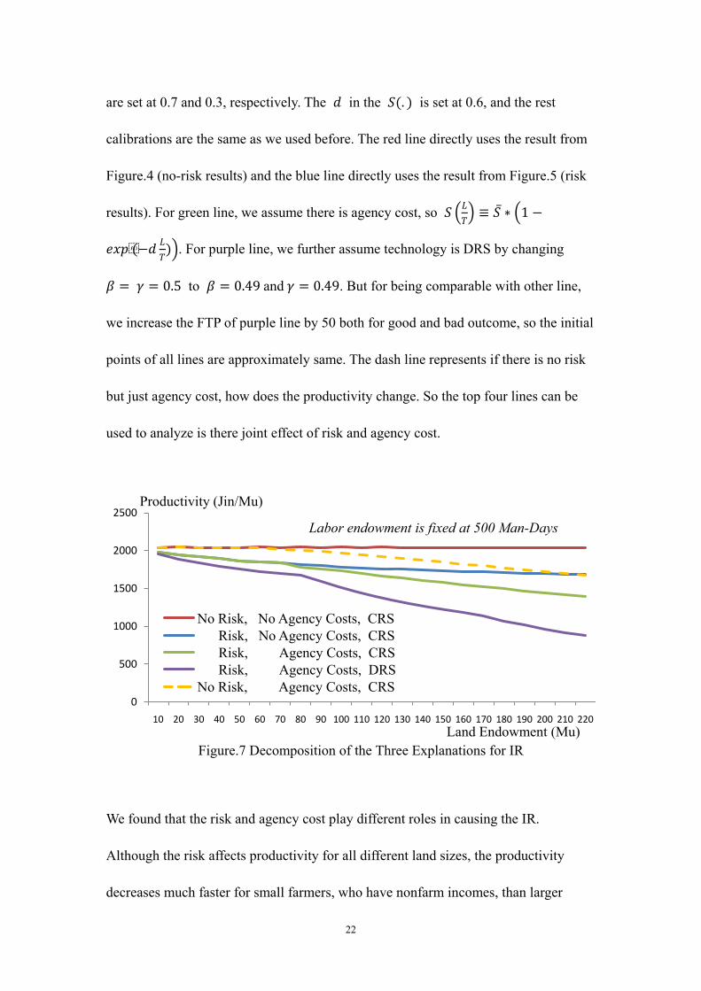
22

are set at 0.7 and 0.3, respectively. The 𝑑𝑑 in the 𝑆𝑆(. ) is set at 0.6, and the rest

calibrations are the same as we used before. The red line directly uses the result from

Figure.4 (no-risk results) and the blue line directly uses the result from Figure.5 (risk

results). For green line, we assume there is agency cost, so 𝑆𝑆 �𝐿𝐿𝑇𝑇� ≡ 𝑆𝑆̅ ∗ �1 −

𝑒𝑒𝑒𝑒𝑒𝑒(−𝑑𝑑 𝐿𝐿𝑇𝑇

)�. For purple line, we further assume technology is DRS by changing

𝛽𝛽 = 𝛾𝛾 = 0.5 to 𝛽𝛽 = 0.49 and 𝛾𝛾 = 0.49. But for being comparable with other line,

we increase the FTP of purple line by 50 both for good and bad outcome, so the initial

points of all lines are approximately same. The dash line represents if there is no risk

but just agency cost, how does the productivity change. So the top four lines can be

used to analyze is there joint effect of risk and agency cost.

We found that the risk and agency cost play different roles in causing the IR.

Although the risk affects productivity for all different land sizes, the productivity

decreases much faster for small farmers, who have nonfarm incomes, than larger

0

500

1000

1500

2000

2500

10 20 30 40 50 60 70 80 90 100 110 120 130 140 150 160 170 180 190 200 210 220

No Risk, No Agency Costs, CRSRisk, No Agency Costs, CRSRisk, Agency Costs, CRSRisk, Agency Costs, DRS

No Risk, Agency Costs, CRS

Productivity (Jin/Mu)

Figure.7 Decomposition of the Three Explanations for IRLand Endowment (Mu)

Labor endowment is fixed at 500 Man-Days

23

farmers according to simulation result. In contrast, the agency cost reduces the

productivity only when farmers have extra lands, i.e. they have to hire labors to work

on their extra lands. Lastly, the DRS can certainly explain IR for all types of farms,

the effect of return to scale purely depends on the parameters, i.e. the nature the

technology.

The orange dash line starts to deviate from red line at 𝑇𝑇� = 60, while the green line

starts to deviate from blue line at 𝑇𝑇� = 70. So the start point of hiring is pushed to

right when the agency cost and risk both exist. The reason can still be explained by

farmer's willingness to balance the investment intensity between risky department and

risk free department. As risk exists, the farm activity becomes less attractive, so the

farmer inclines to reallocate resource (labor input) from risky farm department to risk

free labor department, resulting nonfarm work demand increases, so the starting point

of hiring labor is pushed from 60 mu to 70 mu.

When combining the effects of risk and agency cost, the two factors mitigate each

other's effect in causing IR (such mitigate effect is small, like 20-60 Yuan/mu), not

amplifying each other's effect. The reason could be that the farmer' force or

willingness to balance the risky investment and risk free investment is marginally

decreasing. So when risk already causes the IR, the effect of agency cost on IR

decreases as the farmer becomes less sensitive to one more IR explanation.

24

4. Empirical Testing

The theoretical section shows the how risks causes the IR, and illustrates that the

agricultural insurance can boost farmers' productivity. The following two hypotheses

corresponding to the theoretical findings will be tested using field survey data.

Hypothesis 1: Risk can explain the IR even we control farmers for CRRA. Hypothesis

2: Well-functional insurance market can mitigate the degree of IR.

4.1 Data Description

Right now, three data sets from large scale cross-section household agricultural

production surveys are available. But right now, the following estimation result just

uses the 2013 survey data.

2010, 7 provinces in China, 1353 households, 8% of the sample are insured.

2012, 9 provinces in China, 3332 households, 38% of the sample are insured.

2013, 6 provinces in the northeast and north China, 786 households, 4 agricultural

enterprises, and 55 cooperatives. Among total 845 observations, 47% of the

sample are insured.

4.2 Identification Strategy

To find the joint effect of insurance and land size on farmers’ productivity, the

following econometric model will be estimation:

𝑌𝑌𝑖𝑖𝑖𝑖 = 𝛼𝛼 + 𝛽𝛽𝑇𝑇𝑖𝑖𝑖𝑖 + 𝛾𝛾𝐼𝐼𝑖𝑖𝑖𝑖 + 𝛿𝛿𝑇𝑇𝑖𝑖𝑖𝑖 𝐼𝐼𝑖𝑖𝑖𝑖 + 𝜆𝜆 𝑋𝑋 + 𝜖𝜖𝑖𝑖𝑖𝑖

where 𝑌𝑌𝑖𝑖𝑖𝑖 is the agricultural productivity of individual 𝑖𝑖 in village 𝑖𝑖, measured by

25

revenue per mu (Yuan/Mu); 𝑇𝑇𝑖𝑖𝑖𝑖 represents the land size (Mu) in corresponding

growth season (for some province, there may be two growth seasons); 𝐼𝐼𝑖𝑖𝑖𝑖 indicates

the treatment state, if the farmer purchased insurance, 𝐼𝐼𝑖𝑖𝑖𝑖 = 1, otherwise, 𝐼𝐼𝑖𝑖𝑖𝑖 = 0;

and 𝑇𝑇𝑖𝑖𝑖𝑖 𝐼𝐼𝑖𝑖𝑖𝑖 is the interaction term of the land size and the insurance treatment state.

The above three regressors are variables interested.

The rests, 𝑋𝑋, are controls, including the local average production loss rate (%) in

2013 for controlling local agricultural risk level; local crop average price (Yuan/Jin),

weighted by total crop revenues, for controlling output market disturbance; the

individual non-farm income (1000Yuan) in 2013; the farmers’ wealth level

(1000Yuan); regional dummies (at province level); age (year) and age squared; Plot

Distant to Home (Km); Agricultural Experience (Year); family labor per mu

(Person/mu); Plain Terrain Rate (%); Number of glowing season (#); 2012 household

loss rate (100%); 2012 nonfarm income (1000 Yuan); Gender (1=mal;0=female). .

The Greek letters in the model are the coefficients to be estimated, except the last one

𝜖𝜖𝑖𝑖𝑖𝑖 , which is the error term.

As projected in the conceptual section, large farmers could have lower productivity

than small farmers, therefore, the expected sign of 𝛽𝛽 is negative. Moreover, as after

being insured, farmers will choose more risky portfolios, which supposedly can bring

them higher expected outcomes, hence, in a well-functioning insurance market, the

expected sign of 𝛾𝛾 should be positive. Furthermore, one of the most important

contributions of this study comes from the theoretical finding of the joint effect of

26

insurance and land size on productivity, large farmers will receive more benefits from

being insured. This theoretical finding should be able to be justified by empirically

testing whether the 𝛿𝛿 is positive.

Because higher risk farmers may be more likely to purchase insurance than lower risk

farmers, resulting endogeneity of the insurance purchase variable, 𝐼𝐼𝑖𝑖𝑖𝑖 . To estimate the

model, an instrumental variable has to be used for correcting the endogeneity (using

2SLS). We use insurance policy accessibility, denote as 𝐴𝐴𝑖𝑖 , as an instrumental

variable. 𝐴𝐴𝑖𝑖 = 1 means the village 𝑖𝑖 has insurance policy accessibility, otherwise

𝐴𝐴𝑖𝑖 = 0. Note that, the data do not come from an RCT project, which means 𝐴𝐴𝑖𝑖 may

not be a perfect IV, since it is not randomly assigned to farmers, however, if we can

accept an assumption that the degree of endogeneity from insurance policy is less than

the degree of endogeneity from farms, then, the estimated results are still meaningful

according to Nevo and Rosen (2012) -- the real coefficients 𝛾𝛾 and 𝛿𝛿 can be bound

by using imperfect IV. Particularly in this study, the real value of 𝛾𝛾 and 𝛿𝛿 should be

larger than or equal to the maximum values of my estimated coefficients, respectively,

i.e. 𝛾𝛾 ≥ max{𝛾𝛾�𝑂𝑂𝐿𝐿𝑆𝑆 , 𝛾𝛾�2𝑆𝑆𝐿𝐿𝑆𝑆} and 𝛿𝛿 ≥ max{�̂�𝛿𝑂𝑂𝐿𝐿𝑆𝑆 , �̂�𝛿2𝑆𝑆𝐿𝐿𝑆𝑆}.

As just being mentioned, 2SLS will be employed to estimate the model. Since the

endogenous variable 𝐼𝐼𝑖𝑖𝑖𝑖 is interacted with 𝑇𝑇𝑖𝑖𝑖𝑖 , the equation actually has two

endogenous terms. To fix this problem, we interact the IV, 𝐴𝐴𝑖𝑖 , with 𝐿𝐿𝑖𝑖𝑖𝑖 for creating

a second IV. Then, there are two ways to perform 2SLS. One standard way to run

2SLS with two endogenous terms is to have two regressions in the first stage for

27

getting fitted 𝐼𝐼𝑖𝑖𝑖𝑖� and 𝑇𝑇𝑖𝑖𝑖𝑖 𝐼𝐼𝑖𝑖𝑖𝑖� , respectively, then use them to run the second stage.

However, in this particular model setting, although there are two endogenous terms in

the model, there is essentially only one source of the endogeneity (𝐼𝐼𝑖𝑖𝑖𝑖 ). Using another

regression in the first stage to predict the 𝑇𝑇𝑖𝑖𝑖𝑖 𝐼𝐼𝑖𝑖𝑖𝑖� will lead to a variance reduction in the

fitted regressor in the second stage, resulting in efficiency loss. Therefore, we use an

alternative way to increase efficiency, which only requires one regression in the first

stage to obtain 𝐼𝐼𝑖𝑖𝑖𝑖�, then directly use 𝐼𝐼𝑖𝑖𝑖𝑖� to interact with 𝑇𝑇𝑖𝑖𝑖𝑖 , hence, we have 𝑇𝑇𝑖𝑖𝑖𝑖 𝐼𝐼𝑖𝑖𝑖𝑖� to

act as the second IV for endogenous interaction term 𝑇𝑇𝑖𝑖𝑖𝑖 𝐼𝐼𝑖𝑖𝑖𝑖 . This manually perform

2SLS requires correcting the standard deviation.

4.3 Estimation Results

Table.1 provides the estimation results using improved 2SLS (manually multiply

predicted insurance purchase variable with real land size variable in the 1st stage).

First of all, the general result of model fitting is acceptable. The R-squared ranges

from 0.686 to 0.707, which is an acceptable level considering just using cross-sectional

data. Secondly, all the signs of the estimated coefficients are consistent with

expectations. Furthermore, most estimated coefficients are statistically significant,

especially the key variables.

Three key empirical findings will be discussed based on the estimation (4). First of all,

temporally assume a farmer does not purchase insurance, i.e. 𝑇𝑇𝑖𝑖𝑖𝑖 𝐼𝐼𝑖𝑖𝑖𝑖 = 0, his/her

marginal increase of land size will reduce productivity by 0.7 yuan/mu, so IR exist.

Based on simple algebra using the survey data, if average land size increases by 25%,

28

i.e. roughly 1 hectare, the total agricultural production decreases 1%; if average land

size is doubled, the total production decreases 3.8%. Note that, in 2013, the rate of

China’s national agricultural production increase is only 2.6% according to

government reports.

Secondly, the estimation of 𝛾𝛾�2𝑆𝑆𝐿𝐿𝑆𝑆 justifies our conceptual finding, that farmers with

insurance are more likely to take more risky but profitable decisions, causing

expected productivity to increase. Given the land size at sample mean level,

purchasing insurance can increase productivity more than 276 yuan/mu, accounting

for about 15% of current productivity mean, which is considerable number in

magnitude. If looking at this number from another angle, this 15% productivity can be

considered as an average loss due to farmers’ risk aversion. This finding provides

evidence that developing a well-functioning agricultural insurance market is not only

good for smoothing farmers’ income but also good for increasing agricultural

productivity.

Lastly, the estimated coefficient of the interaction term, �̂�𝛿2𝑆𝑆𝐿𝐿𝑆𝑆 , is positive, which is

consistent with the expectation, that insurance has heterogeneous impact on farmers

(large farmers receive more benefits from insurance). More importantly, 𝛿𝛿�2𝑆𝑆𝐿𝐿𝑆𝑆

𝛽𝛽�2𝑆𝑆𝐿𝐿𝑆𝑆 ≈

94%, i.e. 94% of IR is explained. Therefore, this empirical finding provides a strong

support for urging government to develop a well-functioning agricultural insurance

market in order to secure the national food supply and promote the land market

transformation.

29

Table.1 Improved 2SLS Estimation Results: Effect of Insurance Dependent Variable: Productivity (Yuan/Mu)

(1) (2) (3) (4) SE Robust-SE SE Robust-SE

Key Variables Cultivated Land Size(Mu) -0.701 -0.701 -0.753 -0.753

(0.239)*** (0.327)** (0.259)*** (0.402)* Insurance Purchase (1=Yes; 0=No)

285.8 285.8 276.3 276.3 (103.8)*** (99.49)*** (101.9)*** (98.63)***

Insurance Purchase * Land Size 0.580 0.580 0.705 0.705 (0.218)*** (0.288)** (0.257)*** (0.389)*

Controls Non-Farm Income (1000Yuan) -0.118 -0.118 0.516 0.516 (0.292) (0.335) (1.029) (1.067)

Local Loss Rate (%) -15.96 -15.96 -14.73 -14.73 (1.379)*** (1.610)*** (1.355)*** (1.595)***

Local Crop Price (Yuan/Jin) 771.3 771.3 756.2 756.2 (42.22)*** (41.89)*** (41.42)*** (42.24)***

Wealth (1000Yuan) 0.0834 0.0834 0.0838 0.0838 (0.0567) (0.0445)* (0.0555) (0.0446)*

pcode_dummy2 16.81 16.81 24.44 24.44

(75.32) (70.28) (73.46) (68.68)

pcode_dummy3 223.9 223.9 217.6 217.6

(54.00)*** (48.04)*** (53.26)*** (48.80)***

pcode_dummy4 831.1 831.1 369.0 369.0

(59.30)*** (56.91)*** (114.3)*** (123.6)***

pcode_dummy5 815.0 815.0 352.0 352.0

(83.26)*** (86.11)*** (131.5)*** (147.7)**

pcode_dummy6 894.4 894.4 441.4 441.4

(59.32)*** (65.29)*** (111.9)*** (125.2)***

Loan Time since 2010(#)

-15.02 -15.02

(7.083)** (7.957)*

Age (year)

-36.34 -36.34

(10.50)*** (12.24)***

Age Squared

0.379 0.379

(0.0998)*** (0.115)***

Education (Year)

-5.557 -5.557

(5.075) (4.923)

Plot Distance to Home (km)

-3.585 -3.585

(6.255) (5.152)

Agricultural Experience (Year)

-1.767 -1.767

(2.001) (1.894)

Family Labor Per Mu

17.02 17.02

30

(Person/Mu)

(21.07) (16.30)

Terrain (Plain Terrain Rate) (%)

170.3 170.3

(66.65)** (68.74)**

Number of Growing Season(#)

438.1 438.1

(101.1)*** (119.2)***

2012 HH Yield Loss Rate (100%)

-2.479 -2.479

(1.123)** (0.997)**

2012 Nonfarm Income(1000Yuan)

-0.587 -0.587

(1.065) (1.115)

Gender (1=male;0=female)

230.2 230.2

(102.0)** (94.13)**

Constant 338.6 338.6 484.2 484.2

(86.48)*** (78.62)*** (311.3) (351.0)

Observations 844 844 844 844 R-squared 0.686 0.686 0.707 0.707 Standard errors in parentheses

*** p<0.01, ** p<0.05, * p<0.1

31

Appendix

Appendix.I A General Production Function and the Fixed-Input Assumption

Firstly, write down a general form of C-D production function with three input

elements, 𝑌𝑌 = 𝑓𝑓(𝐸𝐸,𝑋𝑋,𝑇𝑇):

𝑌𝑌 = 𝛼𝛼0𝐸𝐸𝛽𝛽 ��𝑋𝑋𝑖𝑖𝛾𝛾𝑖𝑖

𝑍𝑍

𝑖𝑖=1

�𝑇𝑇𝛾𝛾𝑇𝑇

where 𝑋𝑋𝑖𝑖 is total amount of 𝑖𝑖th material input, such as seeds, fertilizers, pesticides,

etc; 𝑍𝑍 is total number of types of material inputs; 𝑎𝑎0 is a total factor productivity

(TPF); 𝛾𝛾𝑖𝑖 is output elasticity of 𝑖𝑖th material input; and 𝛾𝛾𝑇𝑇 is output elasticity of

land.

One of the important explanations of the IR, rather than the land quality and labor

issues, is that small farms tend to have higher input intensity than large farms (Barrett,

1996; Sen, 1962). In other words, the input per area, denoted as 𝑒𝑒𝑖𝑖 , can be a function

of 𝑇𝑇 (possibly negatively correlated with 𝑇𝑇), i.e. 𝑋𝑋𝑖𝑖 = 𝑒𝑒𝑖𝑖(𝑇𝑇)𝑇𝑇. Therefore:

𝑌𝑌 = 𝛼𝛼0𝐸𝐸𝛽𝛽 ��𝑒𝑒𝑖𝑖(𝑇𝑇)𝛾𝛾𝑖𝑖𝑇𝑇𝛾𝛾𝑖𝑖𝑍𝑍

𝑖𝑖=1

�𝑇𝑇𝛾𝛾𝑇𝑇 = [𝛼𝛼0 �𝑒𝑒𝑖𝑖(𝑇𝑇)𝛾𝛾𝑖𝑖𝑍𝑍

𝑖𝑖=1

]𝐸𝐸𝛽𝛽𝑇𝑇𝛾𝛾𝑇𝑇+∑ 𝛾𝛾𝑖𝑖𝑍𝑍𝑖𝑖

Although, by simulation method, using the general production function form still can

yield results for analysis (function form of 𝑒𝑒𝑖𝑖(𝑇𝑇) need to be specified explicitly).

However, for focusing on risk, it does no harm to simplify the production function by

applying a Fixed Input-Assumption, which means 𝑒𝑒𝑖𝑖(𝑇𝑇) ≡ 𝑒𝑒𝑖𝑖� , therefore:

𝑌𝑌 = [𝛼𝛼0 ��̅�𝑒𝑖𝑖𝛾𝛾𝑖𝑖

𝑍𝑍

𝑖𝑖=1

]𝐸𝐸𝛽𝛽𝑇𝑇𝛾𝛾𝑇𝑇+∑ 𝛾𝛾𝑖𝑖𝑍𝑍𝑖𝑖

Denote a generalized α = 𝛼𝛼0 ∏ �̅�𝑒𝑖𝑖𝛾𝛾𝑖𝑖𝑍𝑍

𝑖𝑖=1 , and a generalized 𝛾𝛾 = 𝛾𝛾𝑇𝑇 + ∑ 𝛾𝛾𝑖𝑖𝑍𝑍𝑖𝑖 , so

simplified production function is: 𝑌𝑌 = 𝛼𝛼𝐸𝐸𝛽𝛽𝑇𝑇𝛾𝛾 ≡ 𝑔𝑔(𝐸𝐸,𝑇𝑇)

32

Appendix.II Mathematical Results of the Basic Model (will be updated in next

version)

33

Appendix.III Risk-Averse Utility Function

To choose a utility function form for building the farmer’s utility maximization

problem (UMP), it is worth to reveal some “secrets” of the risk-averse utility

functions. First of all, Figure.IV1 helps us to better understand the relationship

between the absolute risk aversion (ARA) and relative risk aversion (RRA). It is

easily to show that any smooth risk-averse utility function should have a position in

Figure.IV1, according to the size of the third derivative relative to the two cut-off

values, 𝑈𝑈𝐴𝐴′′′ and 𝑈𝑈𝐵𝐵′′′ , marked in the figure. The “𝑐𝑐” is the final consumption in the

utility function.

The basic findings of Figure.IV1 are that all IARA and CARA utility functions must

be IRRA, but DARA is not necessary to be DRRA. Moreover, all CRRA and DRRA

utility functions must be DARA, but IRRA is not necessary to be IARA. Drawing

Figure.IV1 is useful, since it explains why most of studies agree with that people are

DARA, but there are many diversified conclusions on people’ RRA (Arrow, 1971;

Levy, 1994; Szpiro, 1986)9. Currently, empirical studies find that most of people’s

ARA and RRA locate in the circled area in Figure.IV1. Hence, to choose a utility 9 Many papers try to measure the RRA and obtain various results. Here I only cite three of them to represent the three directions. Arrow (1971) supports IRRA; Szpiro (1986) finds CRRA, and Levy (1994) stands for DRRA.

where 𝑈𝑈𝐴𝐴′′′ = �𝑈𝑈 ′′�2

𝑈𝑈 ′ and 𝑈𝑈𝐵𝐵′′′ = �𝑈𝑈 ′′�2

𝑈𝑈 ′ − 𝑈𝑈 ′′

𝑐𝑐= 𝑈𝑈𝐴𝐴′′′ −

𝑈𝑈 ′′

𝑐𝑐

0

DRRA CRRA IRRA

DARA CARA IARA

𝑈𝑈′′′ 𝑈𝑈𝐴𝐴′′′

𝑈𝑈𝐵𝐵′′′

Figure.IV1 Classification of ARA and RRA for Risk-Averse Utility

34

function for this study, I adopt a DARA utility function.

Secondly, recall that the former studies build a “one to one relationship" between the

types of RRA and the IR, for example, only IRRA results in IR. However, their

conclusion is not complete. If we consider the income share effect (ISE), it can be

shown that both IRRA and CRRA will lead to the IR, and part of DRRA can also

result in the IR. To test whether there is real ISE existing, I assume the farmer’s utility

function is CRRA.

In a word, the utility function I use in this analysis should be DARA and CRRA, i.e.

the function should locate at point 𝑈𝑈𝐵𝐵′′′ in Figure.IV1. The Table.IV1 summarizes

most commonly used utility functions in risk related research. The Isoelastic Utility

(IU) is chosen to continue the following analysis, but note that, the result does not

change if I use the Natural Logarithmic Utility (NLU), and the general form of the

Power Utility (PU) can be used to prove that part of DRRA utility function can also

lead to the IR.

Table.IV1 Common Used Utility Functions in Risk Related Research

Formulation ARA RRA Locations in Figure.IV1

Quadratic Utility (QU)

𝑈𝑈(𝑐𝑐) = 𝜓𝜓𝑐𝑐 − 𝜙𝜙𝑐𝑐2, 𝜓𝜓2𝛿𝛿≥ 𝑐𝑐̅,𝜙𝜙 > 0 IARA IRRA 0-Point

Exponential Utility (EU)

𝑈𝑈(𝑐𝑐) =1 − 𝑒𝑒−𝜓𝜓𝑐𝑐

𝜓𝜓 ,𝜓𝜓 ≠ 0 CARA IRRA Point 𝑈𝑈𝐴𝐴′′′

Power Utility (PU)

35

𝑈𝑈(𝑐𝑐) = �(𝑐𝑐 + 𝜂𝜂)1−𝜓𝜓 − 𝜙𝜙

1 − 𝜓𝜓 ,𝜓𝜓 ≠ 1

𝑙𝑙 𝑙𝑙(𝑐𝑐 + 𝜂𝜂) ,𝜓𝜓 = 1,𝜙𝜙 = 1

� DARA IRRA if 𝜂𝜂>0; CRRA if 𝜂𝜂=0; DRRA if 𝜂𝜂<0

𝑈𝑈𝐴𝐴′′′ -𝑈𝑈𝐵𝐵′′′ if 𝜂𝜂>0; 𝑈𝑈𝐵𝐵′′′ if 𝜂𝜂=0; 𝑈𝑈𝐵𝐵′′′ -∞ if 𝜂𝜂<0

Isoelastic Utility (IU) – A Special form of PU

𝑈𝑈(𝑐𝑐) =𝑐𝑐1−𝜓𝜓

1 − 𝜓𝜓 ,𝜓𝜓 ≠ 1, 𝜂𝜂 = 0,𝜙𝜙 = 0 DARA CRRA Point 𝑈𝑈𝐵𝐵′′′

Natural Logarithmic Utility (NLU) – A Special form of PU

𝑈𝑈(𝑐𝑐) = 𝑙𝑙 𝑙𝑙(𝑐𝑐) ,𝜓𝜓 = 1, 𝜂𝜂 = 0,𝜙𝜙 = 1 DARA CRRA Point 𝑈𝑈𝐵𝐵′′′

Note: 𝑐𝑐 is final consumption; 𝜓𝜓, 𝜂𝜂, and 𝜙𝜙 are parameters.

36

Appendix.IV. Proof of Risk Model Results

First of all, we know that if 𝐶𝐶𝑒𝑒 is zero, then all of 𝑇𝑇� will be invested in production.

Moreover, if 𝐶𝐶𝑒𝑒 is positive, then there will a threshold in 𝑇𝑇� when the 𝑇𝑇� passes this

threshold, the farmer start to waste extra lands, since the marginal benefit starts to be

less than the marginal cost, which is the 𝐶𝐶𝑒𝑒 after that point. We can reasonable

assume that 𝐶𝐶𝑒𝑒 is relatively smell so that no land is wasted, since this is more

realistic case. Also note that, in our simulation, all of lands are used, as 𝑇𝑇� ≤ 220 mu.

In this appendix, I assume 𝑇𝑇 = 𝑇𝑇�, so only 𝐸𝐸 is left as a choice variable.

Note that the objective function is that:

𝑚𝑚𝑎𝑎𝑒𝑒𝐸𝐸

𝐸𝐸[𝑈𝑈(𝐸𝐸)] = 𝑒𝑒 𝑙𝑙𝑙𝑙�𝛼𝛼𝐻𝐻𝐸𝐸𝛽𝛽𝑇𝑇1−𝛽𝛽 + 𝑊𝑊(𝐿𝐿� − 𝐸𝐸) − 𝐶𝐶𝑒𝑒𝑇𝑇� +

(1 − 𝑒𝑒) 𝑙𝑙𝑙𝑙�𝛼𝛼𝐿𝐿𝐸𝐸𝛽𝛽𝑇𝑇1−𝛽𝛽 + 𝑊𝑊(𝐿𝐿� − 𝐸𝐸) − 𝐶𝐶𝑒𝑒𝑇𝑇�

where 𝐸𝐸 is effective labor input. 𝐿𝐿� is labor endowment, so if 𝐸𝐸∗ > 𝐿𝐿�, then the

farmer need to hire labors; if 𝐸𝐸∗ < 𝐿𝐿�, the farmer sell labors.

Labor-Land Elasticity and Inverse Relationship:

Before taking the FOC to find equations for analyzing, it is worth to think about how

to prove the IR. Note that the (expected) productivity per unit land is calculated by:

𝐸𝐸[𝑦𝑦] = �𝑒𝑒𝛼𝛼𝐻𝐻𝐸𝐸∗𝛽𝛽𝑇𝑇1−𝛽𝛽 + (1 − 𝑒𝑒)𝛼𝛼𝐿𝐿𝐸𝐸∗

𝛽𝛽𝑇𝑇1−𝛽𝛽�/𝑇𝑇

= [𝜃𝜃𝛼𝛼𝐻𝐻 + (1 − 𝜃𝜃)𝛼𝛼𝐿𝐿]𝐸𝐸∗𝛽𝛽𝑇𝑇−𝛽𝛽 ≡ 𝛼𝛼𝐸𝐸𝐸𝐸∗𝛽𝛽𝑇𝑇−𝛽𝛽

where 𝛼𝛼𝐸𝐸 is expected TFP.

37

Take derivative of 𝐸𝐸[𝑦𝑦] with respect to 𝑇𝑇, we have:

𝑑𝑑𝐸𝐸[𝑦𝑦]𝑑𝑑𝑇𝑇

= 𝛼𝛼𝐸𝐸[𝛽𝛽𝐸𝐸∗𝛽𝛽−1 𝑑𝑑𝐸𝐸∗

𝑑𝑑𝑇𝑇𝑇𝑇−𝛽𝛽 + (−𝛽𝛽)𝐸𝐸𝛽𝛽𝑇𝑇−𝛽𝛽−1]

= 𝛼𝛼𝐸𝐸𝛽𝛽𝐸𝐸∗𝛽𝛽𝑇𝑇−𝛽𝛽 [𝐸𝐸∗−1 𝑑𝑑𝐸𝐸∗

𝑑𝑑𝑇𝑇− 𝑇𝑇−1]

Therefore, 𝐸𝐸∗−1 𝑑𝑑𝐸𝐸∗

𝑑𝑑𝑇𝑇− 𝑇𝑇−1 determines the sign of 𝑑𝑑𝐸𝐸 [𝑦𝑦]

𝑑𝑑𝑇𝑇. Note that, if 𝐸𝐸∗−1 𝑑𝑑𝐸𝐸∗

𝑑𝑑𝑇𝑇−

𝑇𝑇−1 < 0, which means 𝑑𝑑𝐸𝐸∗

𝑑𝑑𝑇𝑇𝑇𝑇𝐸𝐸

< 1, i.e. if Labor-Land Elasticity, denote as 𝑒𝑒 ≡ 𝑑𝑑𝐸𝐸∗

𝑑𝑑𝑇𝑇𝑇𝑇𝐸𝐸,

is less than one, then IR can be found.

First Order Derivative:

Since we assume that no land will be wasted (𝑇𝑇∗ = 𝑇𝑇�), labor market is available (𝐸𝐸∗

can be larger than 𝐿𝐿�), and production function takes C-D form (𝐸𝐸∗ > 0), so we don't

need to explicitly apply endowment and non-negative constraints when deriving the

results.

Take the FOC of expected utility function with respect to 𝐸𝐸, we have:

𝑑𝑑𝐸𝐸[𝑈𝑈(𝐸𝐸)]𝑑𝑑𝐸𝐸

= 𝑒𝑒𝛽𝛽𝛼𝛼𝐻𝐻𝐸𝐸𝛽𝛽−1𝑇𝑇1−𝛽𝛽 −𝑊𝑊

𝛼𝛼𝐻𝐻𝐸𝐸𝛽𝛽𝑇𝑇1−𝛽𝛽 + 𝑊𝑊(𝐿𝐿� − 𝐸𝐸) − 𝐶𝐶𝑒𝑒𝑇𝑇

+ (1 − 𝑒𝑒)𝛽𝛽𝛼𝛼𝐿𝐿𝐸𝐸𝛽𝛽−1𝑇𝑇1−𝛽𝛽 −𝑊𝑊

𝛼𝛼𝐿𝐿𝐸𝐸𝛽𝛽𝑇𝑇1−𝛽𝛽 + 𝑊𝑊(𝐿𝐿� − 𝐸𝐸) − 𝐶𝐶𝑒𝑒𝑇𝑇= 0

Rearrange the FOC, we get:

𝐸𝐸2𝛽𝛽−1𝑇𝑇2−2𝛽𝛽𝛽𝛽𝛼𝛼𝐻𝐻𝛼𝛼𝐿𝐿 − 𝐸𝐸𝛽𝛽𝑇𝑇1−𝛽𝛽𝑊𝑊𝛼𝛼𝐸𝐸���� + 𝐸𝐸𝛽𝛽−1𝑇𝑇1−𝛽𝛽𝑊𝑊𝐿𝐿�𝛽𝛽𝛼𝛼𝐸𝐸 − 𝐸𝐸𝛽𝛽𝑇𝑇1−𝛽𝛽𝑊𝑊𝛽𝛽𝛼𝛼𝐸𝐸

38

−𝐸𝐸𝛽𝛽−1𝑇𝑇2−𝛽𝛽𝐶𝐶𝑒𝑒𝛽𝛽𝛼𝛼𝐸𝐸 + 𝑊𝑊2𝐸𝐸 −𝑊𝑊2𝐿𝐿� + 𝑊𝑊𝐶𝐶𝑒𝑒𝑇𝑇 = 0

(1)

where 𝛼𝛼𝐸𝐸���� ≡ [(1 − 𝜃𝜃)𝛼𝛼𝐻𝐻 + 𝜃𝜃𝛼𝛼𝐿𝐿]

Total Differentiation of FOC with Respect to 𝑻𝑻:

Take total differentiation of FOC with respect to 𝑇𝑇 at optimal solution level, we

obtain equation (2). Note that 𝐸𝐸∗ is a function of 𝑇𝑇. Denote 𝐸𝐸′ ≡ 𝑑𝑑𝐸𝐸∗

𝑑𝑑𝑇𝑇, and omit the

star mark representing optimal solution in following formulas. the equation (2)

contains 12 terms:

(2𝛽𝛽 − 1)𝐸𝐸2𝛽𝛽−2𝐸𝐸′𝑇𝑇2−2𝛽𝛽 𝛽𝛽𝛼𝛼𝐻𝐻𝛼𝛼𝐿𝐿 + (2 − 2𝛽𝛽)𝐸𝐸2𝛽𝛽−1𝑇𝑇1−2𝛽𝛽𝛽𝛽𝛼𝛼𝐻𝐻𝛼𝛼𝐿𝐿

−𝛽𝛽𝐸𝐸𝛽𝛽−1𝐸𝐸′𝑇𝑇1−𝛽𝛽𝑊𝑊𝛼𝛼𝐸𝐸���� − (1 − 𝛽𝛽)𝐸𝐸𝛽𝛽𝑇𝑇−𝛽𝛽𝑊𝑊𝛼𝛼𝐸𝐸����

+(𝛽𝛽 − 1)𝐸𝐸𝛽𝛽−2𝐸𝐸′𝑇𝑇1−𝛽𝛽𝑊𝑊𝐿𝐿�𝛽𝛽𝛼𝛼𝐸𝐸 + (1 − 𝛽𝛽)𝐸𝐸𝛽𝛽−1𝑇𝑇−𝛽𝛽𝑊𝑊𝐿𝐿�𝛽𝛽𝛼𝛼𝐸𝐸

−𝛽𝛽𝐸𝐸𝛽𝛽−1𝐸𝐸′𝑇𝑇1−𝛽𝛽𝑊𝑊𝛽𝛽𝛼𝛼𝐸𝐸 − (1 − 𝛽𝛽)𝐸𝐸𝛽𝛽𝑇𝑇−𝛽𝛽𝑊𝑊𝛽𝛽𝛼𝛼𝐸𝐸

−(𝛽𝛽 − 1)𝐸𝐸𝛽𝛽−2𝐸𝐸′𝑇𝑇2−𝛽𝛽𝐶𝐶𝑒𝑒𝛽𝛽𝛼𝛼𝐸𝐸 − (2 − 𝛽𝛽)𝐸𝐸𝛽𝛽−1𝑇𝑇1−𝛽𝛽𝐶𝐶𝑒𝑒𝛽𝛽𝛼𝛼𝐸𝐸

+𝑊𝑊2𝐸𝐸′ + 𝑊𝑊𝐶𝐶𝑒𝑒 = 0 (2)

For every term contains 𝐸𝐸′, we can rearrange to obtain the labor-land elasticity

𝑒𝑒 = 𝐸𝐸′ 𝑇𝑇𝐸𝐸, then (2) can be reduced to (3):

𝐸𝐸2𝛽𝛽−1𝑇𝑇1−2𝛽𝛽𝛽𝛽𝛼𝛼𝐻𝐻𝛼𝛼𝐿𝐿[(2𝛽𝛽 − 1)𝑒𝑒 + (2 − 2𝛽𝛽)]

−𝐸𝐸𝛽𝛽𝑇𝑇−𝛽𝛽𝑊𝑊𝛼𝛼𝐸𝐸����[𝛽𝛽𝑒𝑒 + (1 − 𝛽𝛽)]

39

+𝐸𝐸𝛽𝛽−1𝑇𝑇−𝛽𝛽𝑊𝑊𝐿𝐿�𝛽𝛽𝛼𝛼𝐸𝐸(1 − 𝛽𝛽)(1 − 𝑒𝑒)

−𝐸𝐸𝛽𝛽𝑇𝑇−𝛽𝛽𝑊𝑊𝛽𝛽𝛼𝛼𝐸𝐸[𝛽𝛽𝑒𝑒 + (1 − 𝛽𝛽)]

−𝐸𝐸𝛽𝛽−1𝑇𝑇1−𝛽𝛽𝐶𝐶𝑒𝑒𝛽𝛽𝛼𝛼𝐸𝐸[𝑒𝑒(𝛽𝛽 − 1) + (2 − 𝛽𝛽)]

+𝑊𝑊2𝐸𝐸𝑇𝑇−1𝑒𝑒 + 𝑊𝑊𝐶𝐶𝑒𝑒 = 0 (3)

Combining FOC and Total Differentiation Results:

Note that, by FOC equation (1), we have:

𝐸𝐸𝛽𝛽𝑇𝑇1−𝛽𝛽𝑊𝑊𝛼𝛼𝐸𝐸���� = 𝐸𝐸2𝛽𝛽−1𝑇𝑇2−2𝛽𝛽𝛽𝛽𝛼𝛼𝐻𝐻𝛼𝛼𝐿𝐿 + 𝐸𝐸𝛽𝛽−1𝑇𝑇1−𝛽𝛽𝑊𝑊𝐿𝐿�𝛽𝛽𝛼𝛼𝐸𝐸 − 𝐸𝐸𝛽𝛽𝑇𝑇1−𝛽𝛽𝑊𝑊𝛽𝛽𝛼𝛼𝐸𝐸

−𝐸𝐸𝛽𝛽−1𝑇𝑇2−𝛽𝛽𝐶𝐶𝑒𝑒𝛽𝛽𝛼𝛼𝐸𝐸 + 𝑊𝑊2𝐸𝐸 −𝑊𝑊2𝐿𝐿� + 𝑊𝑊𝐶𝐶𝑒𝑒𝑇𝑇 (4)

Substitute (4) into (3), cancelling out 𝛼𝛼𝐸𝐸���� and rearranging, we obtain (5), which is so

far the most reduced and analyzable equation we can get.

𝐸𝐸2𝛽𝛽−1𝑇𝑇1−2𝛽𝛽𝛽𝛽𝛼𝛼𝐻𝐻𝛼𝛼𝐿𝐿(1 − 𝛽𝛽)(1 − 𝑒𝑒) − 𝐸𝐸𝛽𝛽−1𝑇𝑇−𝛽𝛽𝑊𝑊𝐿𝐿�𝛽𝛽𝛼𝛼𝐸𝐸𝑒𝑒

−𝑊𝑊2𝐸𝐸𝑇𝑇−1(1 − 𝛽𝛽)(1 − 𝑒𝑒) + 𝑊𝑊2𝐿𝐿�𝑇𝑇−1(𝛽𝛽𝑒𝑒 + 1 − 𝛽𝛽)

−𝐸𝐸𝛽𝛽−1𝑇𝑇1−𝛽𝛽𝐶𝐶𝑒𝑒𝛽𝛽𝛼𝛼𝐸𝐸(1 − 𝑒𝑒) + 𝑊𝑊𝐶𝐶𝑒𝑒𝛽𝛽(1 − 𝑒𝑒) = 0 (5)

Analysis:

First, we prove that when there is no risk, 𝒆𝒆 = 𝟏𝟏, i.e. no IR will be found.

Proof:

Assuming there is no risk by setting 𝛼𝛼𝑜𝑜 = 𝛼𝛼𝑜𝑜��� = 𝛼𝛼𝐸𝐸 .

40

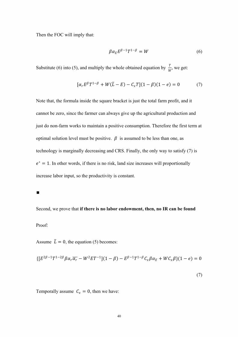
Then the FOC will imply that:

𝛽𝛽𝛼𝛼𝐸𝐸𝐸𝐸𝛽𝛽−1𝑇𝑇1−𝛽𝛽 = 𝑊𝑊 (6)

Substitute (6) into (5), and multiply the whole obtained equation by 𝑇𝑇𝑊𝑊

, we get:

[𝛼𝛼𝑜𝑜𝐸𝐸𝛽𝛽𝑇𝑇1−𝛽𝛽 + 𝑊𝑊(𝐿𝐿� − 𝐸𝐸) − 𝐶𝐶𝑒𝑒𝑇𝑇](1 − 𝛽𝛽)(1 − 𝑒𝑒) = 0 (7)

Note that, the formula inside the square bracket is just the total farm profit, and it

cannot be zero, since the farmer can always give up the agricultural production and

just do non-farm works to maintain a positive consumption. Therefore the first term at

optimal solution level must be positive. 𝛽𝛽 is assumed to be less than one, as

technology is marginally decreasing and CRS. Finally, the only way to satisfy (7) is

𝑒𝑒∗ = 1. In other words, if there is no risk, land size increases will proportionally

increase labor input, so the productivity is constant.

∎

Second, we prove that if there is no labor endowment, then, no IR can be found

Proof:

Assume 𝐿𝐿� = 0, the equation (5) becomes:

{[𝐸𝐸2𝛽𝛽−1𝑇𝑇1−2𝛽𝛽𝛽𝛽𝛼𝛼𝑜𝑜𝛼𝛼𝑜𝑜��� −𝑊𝑊2𝐸𝐸𝑇𝑇−1](1 − 𝛽𝛽) − 𝐸𝐸𝛽𝛽−1𝑇𝑇1−𝛽𝛽𝐶𝐶𝑒𝑒𝛽𝛽𝛼𝛼𝐸𝐸 + 𝑊𝑊𝐶𝐶𝑒𝑒𝛽𝛽}(1 − 𝑒𝑒) = 0

(7)

Temporally assume 𝐶𝐶𝑒𝑒 = 0, then we have:

41

��𝐸𝐸2𝛽𝛽−1𝑇𝑇1−2𝛽𝛽𝛽𝛽𝛼𝛼𝐻𝐻𝛼𝛼𝐿𝐿 −𝑊𝑊2𝐸𝐸𝑇𝑇−1�(1 − 𝛽𝛽)�(1 − 𝑒𝑒) = 0 (8)

Therefore, if the first term equal to zero, then:

𝐸𝐸2𝛽𝛽−1𝑇𝑇1−2𝛽𝛽𝛽𝛽𝛼𝛼𝐻𝐻𝛼𝛼𝐿𝐿 = 𝑊𝑊2𝐸𝐸𝑇𝑇−1 (9)

Rearrange, we get:

𝐸𝐸 = �𝛽𝛽𝛼𝛼𝐻𝐻𝛼𝛼𝐿𝐿𝑊𝑊2 �

12−2𝛽𝛽 𝑇𝑇 (10)

Hence,

𝑒𝑒 = 𝐸𝐸′ 𝑇𝑇𝐸𝐸

=�𝛽𝛽𝛼𝛼𝐻𝐻𝛼𝛼𝐿𝐿

𝑊𝑊2 �1

2−2𝛽𝛽 ∗𝑇𝑇

𝐸𝐸= 1 (11)

If the first term does not equal to zero, the third term has to be zero, which also means

𝑒𝑒 = 1. So, no IR can be found.

Before we relax the assumption on 𝐶𝐶𝑒𝑒 = 0, it is worth to note that the equation (10) is

not the solution of 𝐸𝐸∗. ∀ 𝑐𝑐𝑜𝑜𝑙𝑙𝑠𝑠𝑡𝑡𝑎𝑎𝑙𝑙𝑡𝑡, 𝐸𝐸 = 𝑐𝑐𝑜𝑜𝑙𝑙𝑠𝑠𝑡𝑡𝑎𝑎𝑙𝑙𝑡𝑡 ∗ 𝑇𝑇 will imply 𝑒𝑒 = 1, and

satisfies the equation (8). Therefore, the first term in (8) does not determines the

solution of 𝐸𝐸∗. Using simulation method, it can be shown that when 𝐿𝐿� = 0, 𝐶𝐶𝑒𝑒 = 0:

𝐸𝐸∗ ≈ �𝛽𝛽2𝛼𝛼𝐻𝐻𝛼𝛼𝐿𝐿𝑊𝑊2 �

12−2𝛽𝛽 𝑇𝑇 (12)

Then, we assume 𝐶𝐶𝑒𝑒 > 0. Similar idea as we just explained about (10) and (12), the

first term in (7) does not necessarily determine the value of 𝐸𝐸∗. So, we don't know the

value of the first term, but we do know that 𝑒𝑒 = 1 in the second term in (7) still can

42

solve the equation. Our simulation results also support this conclusion, i.e. 𝐿𝐿� = 0

leads to 𝑒𝑒 = 0.

Therefore, we formally proved that when there is no labor endowment and no fixed

cost, there is no IR, and informally proved that if fixed cost is positive, 𝑒𝑒 = 1 is still

a solution of the model, which indicates no IR can be found.

∎

The Figure.A1 shows simulation results corresponding to the last two mathematically

proved findings.

Unfortunately, so far, we failed in mathematically proving that when labor

endowment is positive, and there is risk, the labor-land elasticity in (5) is less than 1.

Simulation details show that, at optimal solution levels, the sums of the second to

sixth term are always negative, which indicate that the first term must be positive,

i.e. 𝑒𝑒 < 1. For strengthening our findings, we provide Figure.A2, in which there are a

bunch of simulation results with different calibrations. We actually run substantially

43

more simulations than we present here, all of them show IR results.

44

Reference:

Arrow, K. J., 1971, The theory of risk aversion: Essays in the theory of risk-bearing, p. 90-120.

Bardhan, P. K., 1973, Size, productivity, and returns to scale: An analysis of farm-level data in Indian agriculture: The Journal of Political Economy, p. 1370-1386.

Barrett, C. B., 1996, On price risk and the inverse farm size-productivity relationship: Journal of Development Economics, v. 51, p. 193-215.

Benjamin, D., 1995, Can unobserved land quality explain the inverse productivity relationship?: Journal of Development Economics, v. 46, p. 51-84.

Bhalla, S. S., and P. Roy, 1988, Mis-specification in farm productivity analysis: the role of land quality: Oxford Economic Papers, v. 40, p. 55-73.

Carletto, C., S. Savastano, and A. Zezza, 2013, Fact or artifact: The impact of measurement errors on the farm size–productivity relationship: Journal of Development Economics, v. 103, p. 254-261.

Carter, M. R., 1984, Identification of the inverse relationship between farm size and productivity: an empirical analysis of peasant agricultural production: Oxford Economic Papers, p. 131-145.

Carter, M. R., and Y. Yao, 2002, Local versus global separability in agricultural household models: The factor price equalization effect of land transfer rights: American Journal of Agricultural Economics, v. 84, p. 702-715.

Chen, Z., W. E. Huffman, and S. Rozelle, 2011, Inverse relationship between productivity and farm size: the case of China: Contemporary Economic Policy, v. 29, p. 580-592.

CPG, 2013, Guowuyuan Guanyu Jiakuai Fazhan Xiandai Nongye Jing Yi Bu Zeng Qiang Nongcun Fa Zhan Huoli De Yijian (State Council’s Suggestions on Speeding Up Development of Modern Agriculture and Further Strengthening Agricultural Development). Central People’s Government of PRC.

CPG, 2014, Deepening Rural Reforms and Pushing Modernization of Agriculture, Central People’s Government of PRC.

Deininger, K., S. Jin, F. Xia, and J. Huang, 2014, Moving off the farm: Land institutions to facilitate structural transformation and agricultural productivity growth in China: World Development, v. 59, p. 505-520.

Eggleston, K., J. C. Oi, S. Rozelle, A. Sun, A. Walder, and X. Zhou, 2013, Will demographic change slow China's rise?: The Journal of Asian Studies, v. 72, p. 505-518.

Fan, S., and C. Chan‐Kang, 2005, Is small beautiful? Farm size, productivity, and poverty in Asian agriculture: Agricultural Economics, v. 32, p. 135-146.

Feder, G., 1980, Farm size, risk aversion and the adoption of new technology under uncertainty: Oxford Economic Papers, v. 32, p. 263-283.

Feder, G., 1985, The relation between farm size and farm productivity: The role of family labor, supervision and credit constraints: Journal of development economics, v. 18, p. 297-313.

Frisvold, G. B., 1994, Does supervision matter? Some hypothesis tests using Indian farm-level data: Journal of Development Economics, v. 43, p. 217-238.

45

Gorton, M., and S. Davidova, 2004, Farm productivity and efficiency in the CEE applicant countries: a synthesis of results: Agricultural economics, v. 30, p. 1-16.

Jin, S., and K. Deininger, 2009, Land rental markets in the process of rural structural transformation: Productivity and equity impacts from China: Journal of Comparative Economics, v. 37, p. 629-646.

Just, R. E., and D. Zilberman, 1983, Stochastic structure, farm size and technology adoption in developing agriculture: Oxford Economic Papers, v. 35, p. 307-328.

Khan, M. H., and D. R. Maki, 1979, Effects of farm size on economic efficiency: The case of Pakistan: American Journal of Agricultural Economics, v. 61, p. 64-69.

Kung, J. K.-s., 2002, Off-farm labor markets and the emergence of land rental markets in rural China: Journal of Comparative Economics, v. 30, p. 395-414.

Levy, H., 1994, Absolute and relative risk aversion: An experimental study: Journal of Risk and uncertainty, v. 8, p. 289-307.

Li, H., L. Li, B. Wu, and Y. Xiong, 2012, The end of cheap Chinese labor: The Journal of Economic Perspectives, v. 26, p. 57-74.

Mas-Colell, A., M. D. Whinston, and J. R. Green, 1995, Microeconomic theory, v. 1, Oxford university press New York.

Mazumdar, D., 1965, Size of farm and productivity: a problem of Indian peasant agriculture: Economica, v. 32, p. 161-173.

Meng, X., 2012, Labor market outcomes and reforms in China: The Journal of Economic Perspectives, v. 26, p. 75-101.

MOA, 2013, 2013 Nian Guojia Zhichi Liangshi Zengchan Nongmin Zengshou Zhengce Cuoshi (2014 National Policy for Supporting Grain Production and Increasing Farm Income), Ministry of Agriculture, PRC.

MOA, 2014, 2014 Nian Guojia Shenhua Nongcun Gaige, Zhichi Liangshi Shengchan, Cujin Nongmin Zengshou Zhengce Cuoshi (2014 Policy for Deepening Rural Reform, Supporting Grain Production, and Increasing Farm Income). Ministry of Agriculture, PRC.

NDRC, 2009, The Program for Increasing China’s Grain Production Capacity by 50 Billion Kilogram, National Development and Reform Commission.

Rada, N., C. Wang, and L. Qin, 2015, Subsidy or market reform? Rethinking China’s farm consolidation strategy: Food Policy, v. 57, p. 93-103.

Rosenzweig, M. R., and H. P. Binswanger, 1993, Wealth, weather risk and the composition and profitability of agricultural investments: The Economic Journal, v. 103, p. 56-78.

Rozelle, S., J. E. Taylor, and A. DeBrauw, 1999, Migration, remittances, and agricultural productivity in China: The American Economic Review, v. 89, p. 287-291.

Sen, A. K., 1962, An aspect of Indian agriculture: Economic Weekly, v. 14, p. 243-246. Sheng, Y., S. Zhao, K. Nossal, and D. Zhang, 2015, Productivity and farm size in Australian

agriculture: reinvestigating the returns to scale: Australian Journal of Agricultural and Resource Economics, v. 59, p. 16-38.

Srinivasan, T., 1972, Farm size and productivity implications of choice under uncertainty: Sankhyā: The Indian Journal of Statistics, Series B, p. 409-420.

Szpiro, G. G., 1986, Measuring risk aversion: an alternative approach: The Review of Economics and Statistics, p. 156-159.

46

Townsend, R. F., J. Kirsten, and N. Vink, 1998, Farm size, productivity and returns to scale in agriculture revisited: a case study of wine producers in South Africa: Agricultural Economics, v. 19, p. 175-180.

Wang, M., P. Shi, T. Ye, M. Liu, and M. Zhou, 2011, Agriculture insurance in China: History, experience, and lessons learned: International Journal of Disaster Risk Science, v. 2, p. 10-22.

Wang, X., F. Yamauchi, and J. Huang, 2016, Rising wages, mechanization, and the substitution between capital and labor: evidence from small scale farm system in China: Agricultural Economics, v. 47, p. 309-317.

Wenli, F., 2004, Market Failure and Institution Supply of Agriculture Insurance in China [J]: Journal of Finance, v. 4, p. 016.