Agricultural Productivity and Deforestation inBrazil

Juliano AssunçãoPUC-Rio

Molly LipscombUniversity of Virginia

Ahmed Mushfiq MobarakYale University

Dimitri SzermanPUC-Rio

February 28, 2017

Click here for the latest version.

Abstract

Increasing agricultural productivity can have ambiguous effects on forest protec-tion in theory: it can expand the scope of farming, which is detrimental to the forest,but it can also induce farmers to intensify their production. We examine these predic-tions using county-level data from five waves of the Brazilian Census of Agriculture.We identify productivity shocks using the expansion of rural electrification in Brazilduring 1960-2000. We show that electrification increased crop productivity, and farm-ers subsequently both expand farming through frontier land conversion, but also shiftaway from land-intensive activities and into capital- and labor-intensive activities. Thenet effect depends on the county’s land use prior to the increase in agricultural pro-ductivity, but it reduces deforestation in the typical county in the sample.

Keywords: Electricity, Hydro-power, Agriculture, Productivity, Deforestation, Brazil

1

1 Introduction

The rapid loss of tropical forests has been one of the major environmental disasters ofthe last century. Tropical deforestation accounts for nearly 20% of recent global green-house gas emissions (Stern, 2008) and has significant impacts on the world’s biodiversity.The challenge of preventing the loss, and promoting the recovery, of tropical forests isimmense. At its core lies the tension, perceived or real, between conservation goals andeconomic development. Deforestation is intricately tied to decisions on land use for agri-cultural production, which not only is a major source of livelihoods for the world’s poor-est, but also plays an important role in structural transformation of developing societies.Therefore, in balancing development and environmental goals, a key question is to whatextent improvements in agricultural productivity will lead to more or less deforestation.

The link between agricultural productivity and deforestation has been the subject of de-bates in the literature and in policy circles alike (for an early review, see Angelsen andKaimowitz (2001)). Enthusiasts of the Green Revolution argue that increasing yields ulti-mately reduced the pressure of an ever-growing demand for food on the world’s forests.If true, this intensification effect, known as the Borlaug’s hypothesis, provides a “win-win” solution to the conflict between environmental and development objectives that de-veloping countries face. However, improving agricultural productivity gives individualproducers the economic incentives to increase the scope of their farming. This expansioneffect, sometimes referred to as Boserup’s hypotheses, may offset the intensification ef-fect and result in more deforestation. Understanding the extent of each of these effectsis important for policy making in conservation. Forest protection in the tropics is ham-pered by regulators’ inability to enforce fines or bans on deforestation (Burgess et al.,2012). Conservation policies therefore have to account for the preferences of potentialusers of the common pool resource, and focus on strategies that are in the economic inter-est of user groups. Governments and other environmental organizations are increasinglyexperimenting with approaches such as direct payments for ecosystem services (Porras,2012; Jayachandran et al., 2016) or interventions that improve farm productivity.

This paper examines the link between agricultural productivity and deforestation in Brazil.To guide our empirical analysis, we first develop a simple framework that allows for boththe intensification effect as well as the expansion effect. In this framework, farmers en-gage in two activities that are different with respect to their factor intensities – we labelthe land-intensive activity “cattle grazing” and the other activity “crop cultivation”. Thefarmer faces a factor market constraint that limits growth. Any productivity shock biasedtowards cropping will induce farmers to switch into cultivation and decrease the landallocation to grazing. The shift away from the land-intensive activity decreases overall

2

land use, and benefits native vegetation. On the extensive margin, increased agriculturalproductivity induces new people to move into farming, which has the opposite effect ondeforestation. The overall effect on deforestation is therefore theoretically ambiguous, andthis motivates our empirical inquiry.

The empirical exercise uses the impressive expansion of the electricity grid in Brazil dur-ing the period 1960-2000 that electrified many frontier areas and farms as a measure of ashock to agricultural productivity. To address the endogeneity issues inherent in infras-tructure data (where investment may follow demand), we use the IV estimation strategydeveloped in Lipscomb et al. (2013). Using county-level data from the Census of Agri-culture, we first document that electricity access increases productivity of cropping morethan that of cattle grazing. Next, we show that farmland expands following an increase inelectricity infrastructure, but also that farmers leave more of their land in native vegetation(which in Brazil is mostly composed of forests). With both the intensification and expan-sion effects at play, the net effect on overall native vegetation depends on land use beforethe improvement in agricultural productivity: in frontier (consolidated) areas, increasingagricultural productivity has negative (positive) impacts on forests. For the typical county,a 10 percent increase in electricity infrastructure causes the area in native vegetation to in-crease by -0.18 to 2.7 percent, depending on the prior state of native vegetation outsidefarms.

Brazil provides an ideal setting for our study. During our sample period, the enforcementof environmental regulation in Brazil was extremely weak, much like in the rest of thetropics today. Moreover, Brazil is a relevant case study in itself: It is home to the largestportion of rainforest in the world, at the same time that agricultural production grew enor-mously – the country now ranks among the world’s three largest producers of sugarcane,soybeans and maize, and is also the world’s largest exporter of beef. Understanding howthe increases in agricultural productivity interacted with Brazilian forests can yield valu-able lessons to other countries in Latin America and Africa which also ave large portionsof forest, but that have not yet experienced their own Green Revolutions.

Related Literature

Starting with Grossman and Krueger (1991, 1995), a large literature in economics stud-ies the trade-offs between economic development and environmental outcomes. Togetherwith the 1992 World Bank Development Report, these papers popularized the conceptof an Environmental Kuznets Curve (ECK) — an inverted U-shaped relationship betweeneconomic growth and environmental outcomes (see Stern (2004) and Jill L. Caviglia-Harris(2009) for critical reviews of this literature). Part of this literature (eg., Foster and Rosen-

3

zweig (2003)) focuses on the ECK for forests, forming what sometimes is called the for-est transition literature, which broadly shows that afforestation takes place after a certainpoint of economic growth. We contribute to this literature in three ways. First, we providewell-identified effects of one aspect of economic development (agricultural productivity)on forests (native vegetation). The previous literature suffers from methodological con-cerns, by using cross-country regressions or simply time-series correlations. Second, wedo so using Brazil as a case study, whereas most of the previous literature focuses ondeveloped countries. Third, we provide evidence of the positive spillovers between agri-cultural productivity and forests at the local level; time-series evidence on the relationshipbetween yields and area harvested is well-known at least since Dyson (1996).

We also contribute to a literature linking infrastructure and deforestation. Our findingsthat the expansion in the electricity grid had positive effects on deforestation stands incontrast to Pfaff (1999), Cropper et al. (1999) and Cropper et al. (2001), who show thatroad infrastructure aids deforestation in Brazil and Thailand, respectively. Stavins andJaffe (1990) find that flood-control infrastructure projects account for 30 percent of forestedwetland depletion in the Mississippi Valley by affecting private land use decisions.

Our paper is most closely related to papers on agricultural use of electricity and irrigationtechnology in the United States (Lewis and Severnini, 2015; Hornbeck and Keskin, 2014)and in India (Sekhri, 2011), and broadly related to the literatures on technology adoptionin agriculture (BenYishay and Mobarak, 2014; Conley and Udry, 2010) and to a rapidlygrowing literature on the effects of electrification (Dinkelman, 2011; Rud, 2012; Lipscombet al., 2013) and other forms of infrastructure (Duflo and Pande, 2007; Donaldson, ming)on development.

The paper is organized as follows: section 2 discusses historical land use in Brazil, thevast growth in the electricity network during the period 1960-2000, and the expansionof the use of irrigation. Section 3 discusses a simple theoretical model which we use toinvestigate the contrasting impacts of increased agricultural productivity on land use: theincreased intensity of agricultural productivity, versus the potential for expansion acrossincreased land area as agriculture becomes more profitable. Section 4 discusses the twokey datasets that we use–the Census of Agriculture in Brazil, and the Electricity Data fromvarious historical archives in Brazil and elevation maps from USGS. Section 5 discussesour estimation strategy and the instrumental variable technique we employ. Section 6discusses the empirical results, and section 8 concludes.

4

2 Background

Large scale deforestation in Brazil has resulted in a 19% decrease in forest cover in theAmazon since 1970 . This deforestation was, in large part, a result of the widespread ex-pansion of agriculture and cattle grazing (Marguilis, 2004). . The conflict between theforest and agricultural land uses is particularly pronounced in areas of Brazil with lowerdistances and transport costs to major markets: Northern Brazil, the Pantanal and theCerrado (Pfaff, 1997). This expansion in farmland has occurred at the same time as awidespread increase in farm productivity stemming from improved seed varieties, im-proved farming techniques, and increased use of capital in farming. In this section, wediscuss the increase in productivity in the agricultural sector and the reallocation in landuse in farming that has occurred over the past 50 years.

2.1 The Increase in Agricultural Productivity in Brazil

Agricultural productivity in Brazil has increased significantly since 1970, as Brazil closesthe gap between agricultural productivity in Brazil and the US (Viera Filho and Fornazier,2016). This increase in productivity has depended in large part on the ability of farmersto invest in new farming technology, and has varied substantially across regions of Brazil(Viera Filho Santos and Fornazier, 2013).Over the period 1970 to 2002, average yields perhectare increased, and as a result there was also an increase in the area spared from defor-estation (FAO, 2004).

Constraints in Factor Markets The ability to take advantage of productivity improve-ments through new technologies is often dependent on the ability of farmers to investin new capital equipment and to hire workers with higher levels of education than tra-ditional farm labor. One common feature of rural economies in developing countries ispresence of frictions, and ensuing constraints faced by producers in factor markets (Con-ning and Udry, 2007). For example, between 1960 and 2006 at least 80 percent of Brazilianfarmers had no access to external financing of any sort (citation?). Farmers who did ob-tain credit typically used it for short-term loans to finance materials — seeds, fertilizer andpesticides — or transportation, as opposed to long-term investments. Access to other fi-nancial products, such as insurance, is uncommon even today. Agricultural labor marketsin general, and in developing economies in particular, are also plagued by informationalfrictions and strict regulations which create constraints for producers to hire labor. InBrazil, these problems have been compounded by a massive rural-urban migration which

5

decreased labor supply in rural labor markets: the fraction of the population living inrural areas decreased from 64 percent in 1950 to 19 percent in 2000 (citation).

Electricity and Agricultural Productivity Farmers use electricity for various purposesin their agricultural production function including irrigation, processing and storage, pro-duction of fertilizer and pesticides, and production and use of farm machinery (Fluck,1992). For example, many technologies for irrigation and storage of farm production re-quire the use of electricity. Sprinkler irrigation systems, common throughout Brazil, re-quire energy to lift groundwater and distribute it. Although diesel can be used to provideenergy for pumps, using electricity is cheaper not only because of the equipment, but alsobecause of fuel costs. This was particularly true after the oil price shocks in the 1970s, andthe expansion of the electricity grid providing cheap energy from hydropower (WorldBank, 1990; Rud, 2012). In the drier areas of the country, irrigation during the winter sea-son allows for two, and sometimes even three harvests of grains (soybeans, maize, cotton)per growing season, significantly increasing yields.

Electricity also enables farmers to adopt various technologies to process and store theiroutput. Post-harvest handling of grains requires an array of machinery for drying grains,including ventilators and a conveyor belt, which are energy-intensive. Drying grains isimportant as it enables producers to store their output and sell it when market prices aregood, besides adding value to the output. Livestock production can also benefit fromelectricity through mechanized milking, pasteurizing and cooling of dairy products, andpoultry and egg production (Lewis and Severnini, 2015). As we will see, however, thevast majority of the Brazilian cattle herd is for beef production and is not confined, leavingconsiderably less room for electricity to improve cattle grazing productivity.

2.2 Evolution of Land Use in Brazilian Farms

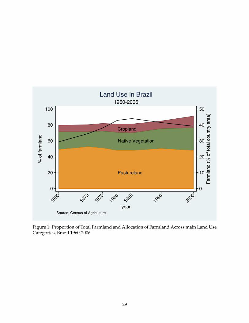
Land use trends over the second half of the twentieth century in Brazil are shown in Fig-ure 1, based on data from the Census of Agriculture, described in more detail in section 4.Farmland expanded considerably, reaching 44 percent of the country’s territory in 1985,from 29 percent in 1960, a 50 percent increase within 25 years, before it started slowly de-creasing. Brazilian farmers allocate their land mainly between pastures, annual crops andnative vegetation; at any point in time between 1960 and 2006, these three categories ac-counted for 80-90 percent of total land in farms.1 As can be seen, there were major changesin the allocation of farmland between these three categories over this period. The share of

1The remaining land use categories include planted forests (timber), perennial crops, water bodies, andunsuitable land.

6

pastureland, which is almost entirely used for cattle grazing, decreased from a peak of 52percent in 1970 to 48 percent of total farmland in 2006, while the shares of cropland andnative vegetation increased from about 9 and 19 percent to 14 and 29 percent, respectively.These trends show a clear expansion of cropland and native vegetation within farmland,at the cost of pastureland and other uses.

There has been substantial growth in the cattle stock in the North and Central West areasof Brazil. In the North, cattle stock more than tripled between 1960 and 1980 and againincreased by 400% by 1990, while in the center West region the cattle stock also increasedby 450%. This expansion in the cattle stock came in part from increased intensity in agri-cultural practices, but in large part the increase came from deforestation. At the same timemany of the farms in the South were converting from cattle herds to soy. (FAO, 2004, p.14).

Native Vegetation in Private Properties Native vegetation is an important componentof our analysis and forms a large component of land use in Brazilian farms. 2 There arepotentially many reasons why producers may decide to keep trees in their properties.Although land is a relatively abundant factor in Brazil, land markets are plagued with fric-tions, from weak property rights to regulations in rental markets. As a result, producersmay leave uncultivated land for the sheer reason of not being able to hire enough laborand capital, nor being able to sell or rent their land. Second, there are regulations man-dating property owners to keep trees in a fraction of their land at least since 1934.3 Thissort of legislation however can hardly explain the observed patterns for the period weanalyze, as its monitoring and enforcement has been an historical challenge in Brazil ingeneral, and in rural areas of the country in particular. Illegal deforestation in the Ama-zon for example only started to be more seriously tackled with command-and-controlpolicies after peaking in 2004, therefore at the very end of our sample period. Third,agro-forestry production is a source of income and livelihood, specially for smallhold-ers. Although this can partially explain the presence of native vegetation in farmland, itcannot explain the increase of native vegetation in farmland at the aggregate level. Overthis period, Brazil’s agriculture became increasingly professional, focused on commodi-ties and export-oriented; the fact that Brazil became the world’s largest soybean producerand exporter is the quintessential example of this trend. Given the increased importance

2The presence of trees among agricultural land is a common feature in the tropics, and not specific toBrazil. Zomer et al. (2014) find that 92 (50) percent of agricultural land in Central America had at least 10(30) percent of tree cover in year 2000.

3This legislation, known as the Brazilian Forest Code, was enacted in 1934 and mandated that everyrural property to keep at least 25 percent of its area in native vegetation, in order to guarantee a stock ofwood fuel. The Forest Code was amended in 1965 and then in 2012 after long public debates. Enforcementof the Forest Code is only now being taken seriously with the help of high-resolution satellite technology,unavailable even in the early 2000’s.

7

of export-oriented commodities, one would have expected the relative share of forestryproduction, and therefore of land allocated to forests in farmland, to decrease during thisperiod. Finally, it is possible that producers realize the production benefits of having bio-diversity in their land, but this is a possibility that we cannot test with our data.

Crop Cultivation and Cattle Grazing As practiced in Brazil, cattle gazing and cropcultivation mix inputs at very different rates. Specifically, cattle grazing is a relativelyland-intensive activity, whereas crop cultivation requires more capital, both physical andhuman. For example, in 2006 the value of machinery and equipment per hectare in thetypical cattle grazing farm was one-sixth of that of a typical crop farm; and crop farmshad eleven times as many workers per hectare than cattle farms. These figures are notsurprising when one notes that only 4 percent of cattle farms use confinement, that only0.2 percent of producers pasteurize the milk they sell, and that the beef cattle heard is fivetimes the dairy cattle herd. At the same time, over 60 percent of the harvested area ofmaize and sugar cane is mechanized, as is virtually all of the soybean production in thecountry. Moreover, crop cultivation demands more human skills than beef cattle graz-ing as practiced in Brazil, requiring experimentation with techniques and inputs, such asseeds and fertilizers. In short, the typical cattle grazing farm requires low levels of capitalinvestments within farm gate when compared to crop farming, a fact that motivates someassumptions in the model we present in Section 3.

8

3 Conceptual Framework

In this section we build a simple, partial-equilibrium theoretical framework inspired bythe salient features of farming and land use in Brazil, with the goal of generating pre-dictions on how a productivity shock in crop cultivation will affect farming choices anddeforestation. To mirror the language in our empirical exercise, we refer to the key pro-ductivity parameter in our model as “availability of electricity”, which is denoted by W.Our model allows farmers to engage in both crop cultivation and cattle grazing becausethese are the two major categories of agricultural activities, as indicated in the previoussection and in the agricultural census data.

The economy is endowed with total land of H which is initially completely covered bynative vegetation. A continuum of individuals reside in this economy, and each decideswhether to become a farmer and convert land to agricultural use. These agents only differby their outside option q, which is their individual-specific opportunity cost of operatinga farm. q ⇠ G, with pdf g. The opportunity cost of farming can be thought of as the wagerate in the non-agricultural sector, which may increase with the availability of electricity,and so we allow W to shift the distribution of outside options in the sense of first-orderstochastic dominance: G(q; bW) G(q; eW), for all bW > eW. The profit from farming activitiesis common across farmers and is denoted P, and the mass of farmers is therefore G(q),where q = {q : q P}.

Each farm is a tract of land of size H, which is fully covered by native vegetation beforefarming activities commence. Each farmer can engage in both crop cultivation and cattlegrazing, and the areas allocated to each type of activity are denoted Hc and Hg, respec-tively. We assume that the production functions for the two activities are similar, exceptthat there is a factor other than land which is more useful in crop cultivation, which wedenote N; we think of N as capital, labor, or a combination of both. Electrification im-proves the productivity of N. Our modeling choice reflects the fact that electrificationenhances the productivity of crop cultivation more than cattle grazing. We assume thefollowing forms for the production functions for crops and cattle grazing: C = WNF(Hc)

and G = F(Hg), with FH > 0, FHH < 0 and FH(0) = •.4

Land and the factor N can be bought in the market at prices p and r, respectively. Farmersare credit constrained and need to fund their expenditures with capital and land fromtheir own resources, M. We normalize the prices of C and G to 15. Thus, each farmer’s

4The factor W only entering the production function for crop but not cattle is merely a modeling simpli-fication. The results we derive only require that electrification benefits crop cultivation relatively more.

5To the extent that commodity prices are exogenous to local conditions, this normalization is innocuous.In any case, making prices endogenous to the (local) productivity shock would not add predictive power to

9

problem can be written as:

maxN,Hc,Hg

P = WNF(Hc) + F(Hg)� rN � p(Hc + Hg) (1)

subject to

rN + p(Hc + Hg) M, (2)

Hc + Hg H. (3)

Our modeling choice reflects the fact that the majority of farmers in Brazil are small andmedium holders who face some factor market constraints in capital, credit or labor whichaffects their ability to hire non-land factors. Since the profit function is linear in N andFH(0) = •, the resource constraint (2) always binds; this is merely a modeling device,and what is essential in this model is that farmers are constrained in their ability to hireN. Land will therefore not be the limiting factor, and the land constraint (3) will typicallynot bind. Again, this focus reflects reality–farming in Brazil expanded into frontier landsthat just needed to be cleared and occupied during our period of study–, and makes themodel informative.

In the Appendix, we show that the optimal land use and production choices for farmers,H⇤

c (W), H⇤g(W), N⇤(W), display the following properties:

∂N⇤

∂W> 0 (4)

∂H⇤c

∂W� 0 (5)

∂H⇤g

∂W< 0 (6)

∂(H⇤c + H⇤

g)

∂W< 0 (7)

The intuition behind equations (4)–(7) is straightforward. Since factor N and land allo-cated to crop cultivation become more productive with electrification, N and Hc move inthe same direction as W in this model, as shown in equations (4) and (5). However, sincethe credit constraint binds, the farmer can only increase land allocated to crop cultivationand/or hire more N in response to an increase in electrification if she decreases land al-located to cattle grazing (equation 6). The total land demand for agricultural purposeswithin the farm, H⇤

c + H⇤g , decreases in response to increases in electrification (equation

7): as farmers switch away from cattle grazing and into crop cultivation, they also spend

this framework.

10

more on N and hence must give up more of Hg than they can increase Hc.6

The net effect of electrification on deforestation depends not only on intensive-marginchanges in land demand within each farm, but also on how the productivity shock inducesextensive-margin changes in the decision to enter the agricultural sector. To analyze thisnet effect, we define the total area of native vegetation, Hv, as the difference betweenthe economy’s total land endowment and farmer’s total land demand for agriculturalpurposes:

Hv = H �Z q

�•(H⇤

c + H⇤g)dG(q) (8)

The derivative of the total area of native vegetation with respect to electrification has twoeffects:

dHvdW

= �d(H⇤

c + H⇤g)

dWG(q)

| {z }>0

� (H⇤c + H⇤

g)G(q)dq

dW| {z }70

(9)

The first term relates to the intensive-margin adjustment, through which electrificationreduces the land demand for each farmer by inducing farmers to shift away from land-intensive cattle grazing activities. The second term is the extensive-margin effect: a pos-itive productivity shock associated with electrification changes the threshold in the dis-tribution of farming opportunity costs below which individuals decide to farm. Whetherthis threshold increases or decreases with electrification depends on the relative magni-tudes of the changes in farming profits and in non-agricultural wages. If electrificationincreases farm profits more than the it increases farmers’ outside option, the extensive-margin adjustment would lead to some deforestation as native vegetation is cleared fornew farms. In this case, the overall effect on native vegetation is ambiguous. Otherwise,farmers’ will leave their land, allowing native vegetation to regrow over time, and the neteffect on deforestation should be unambiguously negative. The net effect on the forest istherefore theoretically ambiguous; it will depend on the relative magnitudes of the twoopposing effects, including the mass of citizens who are on the margin of participation inagriculture. We will examine each of the two (intensive and extensive margin) effects inthe data and infer the net implication of a productivity shock on land demand for agricul-ture and, hence, on deforestation.

6In reality, the price of cropland is higher than the price of pastureland, so the intensification effect mustbe even stronger–and in fact that is what our empirical results show. However, we do not assume differentland prices for each activity precisely to highlight this effect. In the same vein, we assume that electrificationdoes not increase input prices. If electrification increases (decreases) relative price p/r, farmers would adjustby spending more (less) in N and less (more) in Hc + Hg.

11

To sum up, this model makes a few assumptions about the agricultural production func-tion that we can examine in the data, and yields a few further testable predictions, whichwe now summarize.

1. We make the testable assumption that electrification increases crop cultivation pro-ductivity more so than cattle grazing productivity.

2. We assume that farmers face constraints in factor markets. We will provide evi-dence that farmers are credit-constrained, although we cannot rule out that otherconstraints are at work.

3. The model predicts that electrification should lead to greater investments in capital,specifically in capital that raises crop farming productivity.

4. The model predicts that positive productive shocks induce farmers to shift land usefrom land-intensive cattle grazing to N-intensive cultivation.

5. The model highlights that electrification has intensive- and extensive margin effectson the demand for agricultural land. On the intensive margin, it reduces demand foragricultural land through reductions in land demand for cattle grazing. Increases inland demand for crop cultivation, if any, are not enough to offset the reduction inland demand for cattle grazing. The effects on the extensive margin are ambiguous.Land demand – hence, farmland – may or may not increase depending on the rela-tive magnitude of farms’ profits vis-a-vis farmers’ outside option. Hence, the overalleffect on demand for agricultural land is also ambiguous.

12

4 Data

We combine two datasets in order to study the impact of the vast expansion of the elec-tricity network across Brazil from 1960-2000 on agricultural productivity, agricultural in-vestments, and deforestation. First, we use county-level data from the Brazilian Censusof Agriculture in order to track amount of land under cultivation, agricultural inputs, andtotal harvests. Second, we use data assembled by Lipscomb et al. (2013) for measures ofelectricity infrastructure in each decade and an instrumental variable which provides theexogenous variation in electricity access. Table 1 presents summary statistics from thesedatasets.

4.1 Census of Agriculture

The Brazilian Census of Agriculture is a comprehensive and detailed source of data on theuniverse of rural establishments in the country. The definition of a rural establishment isconstant across the waves we use, and is similar to what would be commonly thought ofas a farm: a continuous plot of land under a single operator, with some rural economicactivity – crop, vegetable or flower farming, orchards, animal grazing or forestry. Thereare no restrictions on the size of the plot, tenure, or market participation. Common landsare excluded from this definition, as are domestic backyards and gardens. Throughout thepaper, we refer to a rural establishment simply as a farm. We use county-level data fromthe following 5 waves of the Census of Agriculture: 1970, 1975, 1985, 1996 and 2006.7

During this period, there were significant changes in the borders and number of Brazilianmunicipalities. We follow the methodology of Reis et al (2010), who construct minimumcomparable geographical areas that are constant over this period, allowing for meaningfulcomparison across years. We loosely refer to these areas as counties.

Three sets of outcome variables are central to our analysis. First is the total land in farms(farmland), and how it is split in each of three land use categories: annual crops (cropland),pastures (cropland), and native vegetation. “Native vegetation” in Brazil is mostly com-posed of tropical rainforest although there are other types of forest, as well as Savannah-like portions in the Central parts of the country and a semiarid portion in the Northeast.By design, the Census of Agriculture collects data regarding land within farms, and to thebest of our knowledge, there are no countrywide reliable sources of data on the total areaunder native vegetation for most of our period of analysis. Cropland excludes area for

7This selection was made so as to match the other available sources of data. The first wave of the Censusof Agriculture was carried in 1920. From 1940 to 1970 the Census of Agriculture was decennial. From 1970to 1985 it was carried in 5-year intervals. The last two waves were carried in 1996 and 2006.

13

perennial crops (many of which are in orchards) and includes forage-land. Pastures canbe either natural or planted. Together, these three land use categories account for between81% and 90% of the total land in farms in Brazil during the period 1970-2006. The remain-ing farm area includes orchards, planted forests, buildings and facilities, water bodies andnon-arable land.8

Second, we construct measures to capture farm productivity as well as the productivity ofcrop farming and cattle grazing separately. We measure farm productivity by their grossproduction value divided by total farm area (production per hectare). Gross productionvalue is the market value of all goods produced in farms, including production for ownconsumption. Crop farming productivity is measured in an analogous way: gross cropproduction value of divided by cropland (crop production per hectare). Our main measureof cattle grazing productivity is the farm inventory of cattle heads divided by hectares ofpastureland (heads per hectare). We also breakdown the total cattle herd into beef and dairycattle, and measure dairy cattle productivity as milk production per head of dairy cattle.

A third set of outcome variables is related to the capital stock, irrigation and input usagein farms. For capital stock, we use the number of tractor in a country. For irrigation, wehave the number of farms that use irrigation as well as the irrigated area within farms.Finally, we use spending on fertilizers and pesticides as measures of input usage.

4.2 Electricity Data

The large majority of Brazil’s electricity is based on hydro-power Electricity access is mea-sured based on archival research of the location and date of construction of hydro-powerplants and transmission substations in Brazil from 1950-2000. Reports, inventories, andmaps from Brazil’s major electricity company (Eletrobras) over the period were collected,and the data was consolidated into information about the status of the electricity gridin each decade. Eletrobras made data available on their power plants, transmission lines(which transport electricity from the power plant at which they are generated to the regionin which the electricity will be used), and transmission substations (which take electricityfrom the high voltage transmission lines and convert the power to voltage levels that canbe accepted by distribution lines and used by companies, farms, and households). Thereports include tables cataloging the existing electricity network in order to determinewhere further expansion was necessary over the next decade.

The electricity network in Brazil developed from a base in the more developed and wealthy

8For our purposes in this paper, we explicitly separate planted forests from native forests. The area inplanted forests is small, and bundling the two categories makes no quantitative difference in or results.

14

South in the 1950s and 1960s and spread Southeast in the 1960s and 70s and to the North-east in the 1970s and 1980s. Expansion occurred further westward in the 1980s and 1990s.

As in Lipscomb et al. (2013), we focus on the transmission lines, substations, and genera-tion plants as these are the highest cost components of the infrastructure network and thecomponents most dependent on geographic costs. Distribution networks are very closelylinked with areas where demand for electricity is highest. We merged these datasets,creating a mapping of the location of power plants and transmission substations in eachdecade from 1960 through 2000.

The measure of access to electricity infrastructure is generated as follows: Brazil is dividedinto 33,342 evenly spaced grid points. All grid points within a 50 kilometer radius of thecentroid of a county containing a power plant or transmission substation are assumedto have access to electricity — it is estimated that on average the distribution networksstretch one-hundred kilometers across. The grid points are then aggregated to the countylevel, and the electricity access variable is defined as the proportion of grid points assignedas electrified in a county.

We match census and agricultural census data to electricity data with a time lag betweenthe two since the development of a distribution grid around transmission stations takesseveral years. We match the 1970 Census data to the electricity data for the 1960s; the1975 Census data to the 1970s electricity data; the 1985 Census data to the 1980s electricitydata; the 1995 Census data to the 1990s electricity data; and 2006 Census data to the 2000selectricity data. This gives distribution networks and farms a short period of time toreact to new electricity access so that we observe the changes resulting from expansionin infrastructure.

Because Brazil’s electricity is based primarily on hydro-power, geographic factors playa major role in the expansion of the network. We develop an instrumental variable forelectricity infrastructure based on a prediction of lowest cost areas for expansion in eachdecade in Lipscomb et al. (2013). This instrument is further explained in section 5.1; itis based on using geographic variation to predict the lowest cost expansion path for theelectricity network over time. The instrument is developed using on geographic datacollected from the USGS Hydro1k dataset. The Hydro1k dataset is a hydrographically ac-curate digital elevation map developed from satellite photos of the earth. Using ARCGIS,we then calculate the geographic variables most useful for predicting the cost of buildinga hydro-power plant: maximum and average slope and flow accumulation in the riversnear each of the 33,342 grid points. This data is then matched to each of the 33,342 evenlyspaced grid points for use in the model, and then predicted access is aggregated to thelevel of the 2,184 standardized counties across Brazil.

15

5 Empirical Strategy

In order to identify the impact of access to electricity on deforestation and farm produc-tivity, we use variation in electrification from 1960-2000 and data from the agriculturalcensus on farm productivity and data on deforestation over that period. The principalidentification concern in estimating the effect of access to electricity on farm productivityis that demand variables that attract the government to install new electricity infrastruc-ture in some counties will also be related to farm productivity and deforestation. Forexample, quickly growing nearby cities may increase the demand for electricity, pushingthe government to increase the power network in the area, but it could also increase thedemand for agricultural products and increase the level of capital investments in agricul-ture because of high local demand. This would create an omitted variable bias, and wetherefore need an instrumental variable which includes only variation exogenous to farmproductivity and deforestation.

5.1 Predicting Electricity Expansion Based on Geographic Costs: the

design of the Instrument

Our instrument takes advantage of the fact that hydropower accounts for the majority ofelectricity generation in Brazil. The power potential of a hydropower plant depends onthe distance that the water has to fall from the top to the bottom of the turbine and theamount of water available. Hydropower plants require a steep slope and a large amountof water flow in order to create pressure from the water descending through the turbines.Areas which already have a large natural slope and a significant amount of water flowcan have hydropower turbines installed relatively inexpensively, while areas in which thenatural geography is less suited to hydropower generation must have large dams andhuge flooded areas in order to create enough of a distance for the water to fall that powercan be generated. Creating the conditions for the generation of hydropower in areas notnaturally suited to it imposes costs both from the construction of the dam and from theflooding of the area. This means that topography is highly influential in determining areasthat receive electricity since extending transmission lines is expensive.

We use predicted electricity availability based on the engineering cost of expanding thenetwork to instrument for electrification. We calculate predicted availability at each gridpoint in each decade based on minimization of construction cost for new plants and trans-mission lines at the level of the national budget for new power plants using only geo-graphic characteristics. The instrument is generated using the information considered by

16

engineers when choosing locations for hydropower plants while omitting any demandside information which they might consider. We use the flow accumulation of water andthe maximum and average slope in rivers on a grid of points across Brazil to predict lowcost areas for the generation of electricity. The model varies over time since new powerplants are built first in the lowest cost areas, and later in areas slightly less attractive froman engineering standpoint in order to expand the grid outward. Therefore, we identifyfirst where the most attractive areas are for the generation of hydropower, and allow thenetwork to expand to successively higher cost areas as Brazil invests further in its electric-ity grid from decade to decade.

We use the national budget for electricity plants in each decade based on the size of theexpansion of the actual network in each decade, and predict where these are likely tobe placed given where electricity plants and transmission networks have been placed inpast decades. In the construction of the instrument, we use only topographic character-istics of the land (flow accumulation and slope in rivers) to estimate likely locations fornew electricity access. This instrument is also used in Lipscomb et al. (2013). That paperdemonstrates that electricity expansion had large impacts on both the Human Develop-ment Index and housing values by county.

As described in Lipscomb et al. (2013), there are three key steps to the creation of ourinstrument: first we calculate the budget for plants in each time period based on the ac-tual construction of major dams in each decade across Brazil. Second, we generate a costvariable that ranks potential locations by geographic suitability. We base our suitabilitypredictions on geographic factors of areas where hydropower plants were actually built.Finally, following the prediction on estimated construction site for each dam, we generatean estimated transmission network flowing from the new plants.

The budget of electricity plants is generated based on the actual construction of majorelectricity plants in Brazil over the period. This allows us to model greater expansion ofelectricity in years in which the national government decided to expand production ofelectricity, and reduced expansion in years in which the government budgeted for fewernew plants.

In order to rank the suitability of the different sites, we generate hydrographic variablesusing the USGS Hydro1k dataset. We generate weights for hydrographic variables usingthe actual placement of hydropower plants in Brazil (for robustness we have comparedthese weights to those generated using US hydropower plants, and we arrive at similarresults). The cost parameters are derived using probit regressions in which the dependentvariable is an indicator for whether a location has a dam built on it at the end of thesample period (2000), and the explanatory variables are the topographic measures. Steep

17

gradients and high water availability are key factors reducing dam costs.

The Matlab model then begins by placing the new budgeted hydropower plants for thedecade at grid points with the predicted lowest cost from among those grid points thatare not already predicted to have electricity. The model then predicts transmission linesflowing out from each plant. All plants are assumed to have the same generation capac-ity, as we make no assumption on demand in various areas, so we make the simplifyingassumption that each plant has two transmission substations attached to it. We minimizethe cost of the transmission lines based on land slope and length. We then assume thatall grid points within 50km of a predicted plant or predicted transmission substation arecovered by distribution networks.

In later decades, we take the existing predicted network as given and estimate additionalplants and transmission lines as locating in the next lowest cost areas. We then estimatethe coverage of electricity access in a county by estimating average coverage of grid pointswith predicted electricity across the county.

The key potential identification concern related to this instrumental variables estimationstrategy would be if the geographic costs for expanding electricity access also affectedthe productivity of agriculture or the attractiveness of deforesting new areas. While vari-ables like water access and slope could affect agricultural productivity in a cross-sectionalframework, our identifying variation results from variation in whether the cost param-eter of a gridpoint is low enough to make it among the low cost budgeted points in agiven decade. This generates a non-linearity in chosen gridpoints across decades and isdifferent from a simple ranking of lowest to highest cost gridpoints. Our identification istherefore based on discrete jumps between thresholds of suitability for electricity accessbetween decades. The time variation in our instrument allows us to use fixed effects toseparately control for factors directly impacting the suitability of land for agriculture sothat our estimates are the direct impact of electricity on agricultural productivity.

5.2 Estimation Strategy

We estimate the effect of electrification on the productivity of rural establishments overthe period 1960 to 2000 using county-level data. We are interested in running regressionsof the form:

Yct = ac + gt + bEc,t + #ct, (10)

18

where Yct is the outcome of interest in county c at time t, ac is a county fixed-effect, gt is atime fixed-effect, and Ec,t is the proportion of grid points in county c that are electrified inperiod t – that is, Ec,t is our measure of actual electricity infrastructure.

The main concern with (10) is that, even controlling for time and year fixed-effects, theevolution of electricity infrastructure is likely to be endogenous to a various factors alsoaffecting the evolution of farm productivity. This causes OLS estimates to be biased.

We therefore use an instrumental variable (IV) approach, making use of the instrumentdescribed in Section 5.1. Specifically, we use a 2SLS model where the first stage is:

Ect = a1c + g2

t + qZc,t + hct, (11)

where Zct is the fraction of grid points in county c predicted to be electrified by the fore-casting model (relying only on the exogenous variation from the geographic cost variableschanging according to the budgeted amount of infrastructure in each decade) at time t.The second stage is:

Yct = a2c + g2

t + bbEc,t + #2ct, (12)

where bEc,t is obtained from the first stage regression (11). Note that both Zc,t and Ec,t areconstructed by aggregating grid points within the county. Since the number of grid pointsvary in each county, we weight regressions using county area as weights. In all specifi-cations, we cluster standard errors at the county level in order to avoid under-estimatingstandard errors as a result of serial correlation in electrification.

Our IV strategy corrects for the bias introduced by the endogenous placement of elec-tricity infrastructure by isolating the impact of determinants of the electricity grid evolu-tion unrelated to farm productivity. We present a variety of robustness checks in table 4,demonstrating that our estimates do not vary with the addition of geographic trends andother controls.

19

6 Empirical Results

6.1 First-stage results

Table 2 shows the first-stage results of our main analysis. As explained in section 4, ourinstrument is based on a engineering model that takes various inputs. Columns 1–3 showdifferent specifications controlling directly for some of these inputs. In addition to countyfixed-effects, which are included in all specifications in Table 2, column 1 uses year-fixedeffects. The modeled electricity availability is highly correlated with actual electricityinfrastructure, and this correlation is significant at the 1 percent level. Column 2 addsAmazon-specific year dummies to flexibly control for the region’s time trend, which hassignificantly differed from that of the rest of the country. The point estimates decreasesfrom from 0.326 to 0.265, but remains significant at the 1 percent level. Column 3 adds in-teractions of our water flow and river gradient measures with year dummies. The changesin the point estimate and standard error are negligible and, for the rest of the paper, wemaintain the specification of column 2 as our preferred specification. In columns 4 and 5,we check that both our modeled instrument and measure of electricity infrastructure areindeed correlated with actual electricity provision as captured by the Census of Agricul-ture. The correlations are strongly significant and have similar magnitudes on the meanas those of column 2.

6.2 The effects of electricity on agricultural productivity

We start our empirical exercise by examining a central assumption of our framework,namely that the arrival of electricity is as a positive productivity shock to agriculture andthat it is biased towards to crop cultivation. Table 3 reports the main effects of increasingelectricity infrastructure on agricultural productivity. Columns 1–3 show respectively theOLS, reduced form, and IV estimates when the dependent variable is the log of agricul-ture production value per hectare of farmland. The IV estimate is larger than the OLSestimate and implies that a 10 percent increase in electricity availability increases agri-cultural productivity by 24 percent, and this result is significant at the 1 percent level.Next, we analyze separately the effects on crop cultivation and cattle grazing productiv-ity. Columns 4–6 show results when the dependent variable is the log of crop productionvalue per hectare of cropland. The IV estimate implies that a 10 percentage-point increasein electricity infrastructure increases crop productivity by 24.3 percent, and this effect issignificant at the 1 percent level. The high impact of electricity on crop cultivation pro-ductivity is mirrored by a low impact on cattle grazing productivity. Columns 7–9 show

20

the effects of electricity on log of the value of cattle production per hectare of pastureland.The IV estimate in column 9 implies that a 10 percentage-point increase in electricity leadsto a 12-percent increase in this measure of productivity. Not only this is a much lowerimpact than that for crop cultivation, but the statistical significance is also much lower.

In sum, the arrival of electricity infrastructure in a county significantly increases produc-tivity in crop cultivation, but not in cattle grazing. Section 6.2.1 below gives further ev-idence that the effect of electricity on cattle grazing productivity is small or negligible,supporting our interpretation that the arrival of electricity can be thought of as a produc-tivity shock to crop cultivation, but not to cattle grazing.

6.2.1 Effects of electricity on cattle grazing productivity

To build confidence that electricity has little impact on cattle grazing productivity, Table4 looks at the effect of electricity on alternative measures of cattle-related productivity.9

Columns 1 and 2 show that the fraction of livestock production on overall farm produc-tion decreases with electrification. This is consistent with the results from Table 3 thatelectrification increases productivity in crop cultivation relative to cattle grazing. The next4 columns use alternative measures of cattle grazing productivity. In columns 3 and 4, thedependent variable is the stocking ratio—heads of cattle per hectare of pastureland.10 Incolumns 5 and 6, the dependent variable is fraction of young herd on overall herd, a proxyfor cattle turnover – the idea being that the higher the turnover, the more productive thefarm is. The results show that according to these alternative measures, electrification hasno effect on cattle grazing productivity.

As explained in section 2, electricity can have effects on dairy activities by allowing formechanical milking and refrigeration. To explore this possibility, columns 7 and 8 look atdairy cattle productivity as measured by milk production per dairy call. The IV estimatein column 8 implies that a 10 percent increase in electricity increases milk production by56 litters per dairy cow, a 5.8 percent effect on the mean. This effect does not seem tobe strong enough to induce producers to change their herd’s composition towards dairycattle. We can see this in columns 9 and 10, where the dependent variable is the fraction ofdairy cattle on the herd. The IV coefficient implies that a 10 percent increase in electricity

9Ideally one would measure cattle grazing productivity as kilos per hectare per year. Unfortunately, tothe best of our knowledge this measure is not available from any data sources, and heads per hectare is thebest measure we can use.

10Unlike production value per hectare, heads per hectare does not capture price effects. This is an ad-vantage because beef markets tend to be local, and electricity may raise local demand for beef throughincreased population and income. In turn, increased demand may translate to higher prices, spuriouslyincreasing measures of productivity that .

21

increases the proportion of dairy cows 0.65 percentage point, a small effect on the mean. Insum, the effect of electrification on dairy cattle productivity, while sizable, is not sufficientto induce producers to change their herd composition, having therefore little effect on theaggregate cattle grazing productivity.

6.3 Changes in Land Use and Production Decisions

In this section we examine the effects of electrification on producers’ land use decisions.In our conceptual framework, farmers to switch into crop cultivation and allocating lessland to cattle grazing after receiving a productivity shock. Because of differences in land-intensity, the model predicts that overall land demand for agricultural purposes reducesin the intensive margin. But by making agriculture more attractive, the arrival of elec-tricity may also increase land demand in the extensive margin, leading to an expansion offarmland. We therefore analyze the effect of electrification on the two adjustment margins.

6.3.1 Effects on land use

Table 5 shows the effects of electrification on land allocation. Columns 1 and 2 examinethe extensive margin effects by using the proportion of farmland in the county area as thedependent variable. The IV estimate implies that the share of farmland increases by 2.88percentage points following a 10 percentage point increase in electricity infrastructure,and this effect is statistically significant at the 1 percent level.

Next, we turn to land allocation within farms. In columns 3 and 4 of the table, we seethat the share of pastures in the county’s farmland decreases with electricity infrastruc-ture. The IV estimate in column 4 implies that the share of pastures in farmland decreasesby 3.29 percentage points following a 10 percentage point increase in electricity, a sizableand significant effect of 10 percent on the mean. Columns 5 and 6 show the same anal-ysis for cropland, and find a small and not statistically significant effect. These resultsare consistent with our model’s predictions in two ways. First, although we do not findevidence that cropland relative to farmland expands with the arrival of electricity, the re-sults clearly show that cropland relative to pastureland expands, and that is the substantiveprediction of the model presented in section 3. Second, because crop cultivation requiresnon-land factors, the decrease in pastureland should be greater than the correspondingincrease in cropland. Moreover, the relative increase in cropland is not surprising givenprevious results that electricity increases crop farming productivity relative to cattle graz-ing productivity. In section 6.3.2 below, we show that electrification has effects on the cropmix, which partially explains the small effect on overall cropland.

22

The effect on native vegetation within farms, shown in columns 7 and 8 of Table 5, mirrorsthe difference between the effects on shares of pastureland and cropland. The IV estimateimplies that increasing electrification in a county by 10 percentage-points causes the shareof native vegetation within rural establishments to increase by 3.17 percentage points. Oneimportant aspect to this result is that it does not imply that farmland is reforested follow-ing an increase in electrification. Rather, it means that farmers in counties with increasedelectricity infrastructure deforest less than they would have in the counterfactual scenariowhere electrification does not increase. In line with our model’s predictions, the positiveeffect on native vegetation inside farms contrasts with the potentially negative effect ofelectrification on native vegetation outside farms.

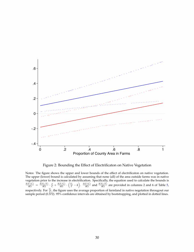
To calculate the effect of electricity on overall native vegetation, one needs to make as-sumptions about the state of native vegetation outside farms prior to the arrival of elec-tricity. At given proportions of farmland in the county area and native vegetation withinfarms, assuming that all land outside farms is covered (not covered) with native vegeta-tion yields the lower (upper) bound of the effect.11 Figure 2 illustrates the bounds for theeffect of electricity on overall native vegetation at varying proportions of farmland in thecounty area using the estimates obtained from table 5, along with confidence intervals ob-tained through bootstrapping. At the sample averages, the effect of a 10 percentage pointincrease in electricity infrastructure on the share of native vegetation ranges from -0.18percentage points (s.e. 0.100) to 2.7 (s.e. 0.087) percentage points, depending on the initialstate of native vegetation outside farms. In “frontier counties” – i.e., counties with littlefarmland as a proportion of the overall area – increasing agricultural productivity tendsto increase deforestation.

Long-run One may wonder if the increase in native vegetation within farms concomi-tantly with the expansion of farmland is not just a first step towards cutting down trees inthe long run. To investigate the impact of electrification in land use choices, we forward-lag the dependent variable by one decade.12 Appendix Table 6 shows that the resultsremain largely unchanged, suggesting that these are not just short-run effects. In fact, thebounds on the effect of electricity in overall native vegetation implied by Table 6 are now

11To see this, write V = VI + VO, where V is the overall area in native vegetation, VI is native vegetationinside farms, and VO is native vegetation outside farms. V0 can be written as k(C � F), where C is the countyarea, F is the area in farmland, and k 2 [0, 1] is the proportion of the area outside farms in native vegetation.Algebraic manipulations and differentiating both sides with respect to W yields ∂(V/C)

∂W = ∂(VI /F)∂W · F

C +∂(F/C)

∂W ·⇣

VIF � k

⌘. To calculate the bounds on the effect of electricity on overall native vegetation, we use the

estimated ∂(VI /F)∂W and ∂(F/C)

∂W from Table 5, as well as the sample averages for FC and VI

F .12As described in section 4, the outcome variables from the Census of Agriculture are already lagged, to

allow for the impacts of electricity to kick in.

23

tighter, with a positive lower bound, suggesting that, if anything, increasing agriculturalproductivity has an even stronger effect in reducing deforestation in the long run.

6.3.2 Effects on crop choices

The substantive prediction of our stylized model is that, following a productivity shock,farmers will substitute away from activities that benefit less from the shock. That predic-tion should be true not only between cattle grazing and crops cultivation, but also acrosscrops that benefit differently from the shock. We therefore analyze effects of electrificationon the composition of different crops choices. Specifically, we investigate the effects ofelectrification separately on grains and cassava. Grains – which include soybeans, maize,cotton and rice – are the high-productive, capital-intensive cash crops that Brazilian farm-ers grow, and the ones that benefit the most from energy-intensive inputs. In contrast,cassava is a staple, commonly grown a subsistence crop across Brazil and relatively moreland-intensive than grains.

Table 7 reports the results. The IV estimate in column 2 implies that grain productionincreases by 32 percent following a 10 percentage point increase in electricity infrastruc-ture, and this estimate is significant at the 1 percent level. In contrast, the IV estimate forcassava production is not statistically significant and in any case has a negligible effectsize. Looking at the land allocated to each of the crops, the IV estimates again imply thatfarmers allocate more land into grains: the IV estimates in columns 4 and 6 show thatfarmers allocate more land to grains and less land to cassava, both in absolute terms andrelative to overall farmland, following arrival of electricity infrastructure. To sum up, theshift from land-intensive towards capital-intensive activities happens also between crops,and not only between cattle grazing and crops.

The results shown in Table 7 also help explaining why we see little or no effect of electri-fication on cropland relative to overall farmland, despite the increased crop productivity.By changing the crop mix towards less land-intensive crops, farmer keep overall croplandstable while responding to the productivity shock.

6.4 Mechanism: increased capital and input usage in crop cultivation

One important part of our model’s mechanism is that electrification should lead to greaterinvestments in capital, specifically in capital that raises crop farming productivity. In sec-tion 2, we highlighted that irrigation and grain storage are two energy-intensive technolo-gies that benefit crop farmers but not cattle ranchers. We now present results that support

24

this story and build confidence that it can explain the mechanisms underlying our results.Specifically, we examine whether farmers use more capital and inputs that are comple-ments to those technologies, such as irrigation, tractors, and fertilizers.

Table 8 presents the effects of electrification on usage of capital and inputs that usedmostly in crop cultivation. Column 1 shows that more farms adopt irrigation as electricitybecomes available. The effect in grain storage capacity and in the number of tractors farm-ers use is also large, as shown in columns 2 and 3, respectively. Finally, columns 4 and 5show that farmers spend more on fertilizers and pesticides per hectare of farmland. Notonly these results are consistent with the intensification effect that is the key mechanismthat behind our main result, but they also support the story that increased electricity in-frastructure enables farmers to adopt technologies and employ capital that would not befeasible otherwise. The increase in crop cultivation productivity is accompanied by largeramounts of capital, fertilizers and pesticides.

6.5 Robustness

As explained in section 4, our instrument uses cross-sectional variation from geographicalfactors, and time-series variation from the national budget for construction of electricityinfrastructure and suitability ranks that introduce discontinuities on the order in whichnew infrastructure is built. Including county fixed-effects isolates any pure cross-sectionvariation. To further mitigate concerns that our instrument uses invalid variation for deal-ing of the endogeneity problems of grid placement, Appendix Tables 9 and ?? presentresults of a sensitivity test where we use all possible combinations of our instrument’scomponents as explicit controls in the second-stage regressions, on top of county fixed-effects and decade dummies. Each row of the tables reports a different specification ofa 2SLS regression. Appendix Table 9 assesses the sensitivity of the results from table 3and shows that both the main result of Table 3 — that electricity affects crop cultivationproductivity, but not cattle grazing productivity — survives all the different specificationsand, in fact, may even get stronger in alternative specifications. Appendix table ?? doesthe same for 5, and shows that both the extensive and intensive margin effects are robustto different specifications.

25

7 Discussion on alternative mechanisms

Our stylized model in section 3 offers an explanation for the empirically observed links be-tween electricity, agricultural productivity and deforestation. There are alternative mech-anisms that could explain the empirical regularities that we document, and we now turnto a discussion of those.

Demand for Forest products One alternative explanation for the positive link betweenelectricity and forests, is through a rise in demand for forestry products induced by anincrease in income and, more broadly, development (Lipscomb et al., 2013). Foster andRosenzweig (2003) argue that such demand mechanism was central to explain the positiveassociation between income and forest in India, as well as in a panel of countries. Oneimportant condition for this mechanism to be captured empirically is that local demandfor forestry products must be met by local supply. Thus, in their panel of countries Fosterand Rosenzweig (2003) find that a positive association between income and forest growthfor closed economies – Brazil included – but not for open economies. We therefore askthe question: did the shift in land use toward forests come from increases in demand forforest products?

We answer this question in Table 10. In columns 1 and 2 the dependent variable is the logof the total value of forestry goods produced. Both the OLS and IV estimates are negative,and the IV estimate is not statistically significant, indicating that production of forestryproducts does not increase with electricity, despite the increase in native vegetation doc-umented in Table 5. Forestry goods however are very heterogeneous, ranging from wildfruits to timber. In columns 3 and 4 we focus on the production of wood-related products– fuelwood, charcoal and timber. The IV estimate is now positive, but not statisticallysignificant. In columns 5 and 6 we ask whether producers make a more intensive useof the forests in their property — a natural thing to do when faced with rising demandfor forestry products – and use the log of the production value of forestry produces perhectare of forest area. The negative OLS and IV estimates suggest that the rise in forestarea within farmland outpaces their direct economic exploration. Finally, we ask whetherproducers actively plant more forests, presumably to meet demand for products that can-not be produced with native species, and use the share of planted forests in farmland asthe dependent variable in columns 7 and 8. Both the OLS and IV estimates are small inmagnitude and non-significant. To sum up, we find no evidence that the demand channelto be driving the growth of native vegetation in Brazil for the period we analyze.

26

Substitution of fuelwood for electricity An argument that runs in the opposite direc-tion of Foster and Rosensweig’s is that electricity may have induced households and firmsto switch away from wood-based fuels, reducing the pace of wood extraction and hencedeforestation. This could result in a positive link between electricity and native vegetationin the data. We argue that this alternative mechanism is unlikely to have played a relevantrole, at least locally, for three reasons.

First, electricity did not replace wood-based fuels in the residential sector, which ac-counted for 70 percent of the firewood consumption in 1970. Whereas household con-sumption of wood-based energy reduced by 50 percent between 1970 and 2006, this re-duction was due to the dissemination of bottled liquefied petroleum gas—a fossil fuelobtained from petroleum or natural gas with little or no use of electricity—, which grad-ually replaced firewood as a cooking fuel. Whereas we cannot formally test this due todata limitations, aggregate data make this point clear: In 1970, 49 percent of householdsused firewood, and 43 percent used bottled LPG for cooking, according to Census data.By 1991 (the last Census to inquire about cooking fuel), 71 percent of households used bot-tled LPG, and 13 percent used only firewood, with a further 14 percent using both bottledLPG and firewood. Electric stoves on the other hand have never been adopted in Brazil.In 1970, only 0.08 percent of households declared using electricity for cooking accordingto Census data, whereas in 1991 respondents did not even have the option to choose “elec-tricity”, which would be under the “other” category, chosen again by 0.08 percent of thehouseholds.

Second, firewood has virtually never been used to generate electricity directly in Brazil.During the period we study, at most 0.75 percent of the energy content of firewood wasused to generate electricity (BRASIL, 2007). Thermal generation in Brazil has typicallyused fossil fuels. Therefore, the hydropower-based electric grid expansion in Brazil didnot directly replace firewood for electricity generation. While in a counterfactual scenariowithout electricity expansion it is possible that aggregate firewood consumption wouldhave increased, there is no evidence that electricity replaced firewood locally, because thisis the variation we use to identify the link between electricity and deforestation.

27

8 Conclusion

We provide evidence that an increase in agricultural productivity can be good for forests.We find that rural properties in counties where electricity infrastructure increases expe-rience more growth in native vegetation than farms located in counties where electricitydid not expand. This effect is persistent, and is consistent with an intensification storywhereby producers substitute away from land-intensive cattle grazing and into crop cul-tivation. Producers also shift away from other subsistence, land-intensive crops, such ascassava and increase the area of capital-intensive crops, such as grains.

We interpret our results as supportive for a more subtle version of the Borlaug Hypoth-esis. The subtlety comes from the fact that increases in agricultural production alone arenot able to prevent farmland to expand; in our story, frictions in factor markets — suchas credit or (local) labor markets — prevent producers to fully explore their land, leavingroom for native vegetation. In absence of such frictions, it is likely that farmland expan-sion would dominate the intensification effect, leading to more forest loss. Yet, given thewidespread presence of frictions in tropical rural economies, these findings are relevantfor contexts other than the Brazilian case.

However, by using variation at the county level only, our analysis ignores the more tra-ditional underestimates the positive effects of agricultural productivity on conservation.Because Brazil is a major commodity producer–“the world’s food basket”–, it is likelythat an increase in Brazilian agricultural productivity has the potential to spare land foragriculture in other countries.

Our results have important implications for policy making in conservation. Forest protec-tion in the tropics is hampered by regulators’ inability to enforce fines or bans on defor-estation. Conservation policies therefore have to account for the preferences of potentialusers of the common pool resource, and focus on strategies that are in the economic inter-est of user groups. Governments and other environmental organizations are increasinglyexperimenting with approaches such as direct payments for ecosystem services13 or inter-ventions that improve farm productivity.

13Several developing countries are already beginning to implement payments for environmental ser-vices, including Costa Rica, Brazil, Vietnam, and Uganda(Porras, 2012).

28

Pastureland

Native Vegetation

Cropland

0

10

20

30

40

50

Farm

land

(% o

f tot

al c

ount

ry a

rea)

0

20

40

60

80

100

% o

f far

mla

nd

1960

1970

1975

1980

1985

1995

2006

yearSource: Census of Agriculture

1960-2006Land Use in Brazil

Figure 1: Proportion of Total Farmland and Allocation of Farmland Across main Land UseCategories, Brazil 1960-2006

29

-.4

-.2

0

.2

.4

.6

0 .2 .4 .6 .8 1Proportion of County Area in Farms

Figure 2: Bounding the Effect of Electrificaton on Native Vegetation

Notes: The figure shows the upper and lower bounds of the effect of electrificaton on native vegetation.The upper (lower) bound is calculated by assuming that none (all) of the area outside farms was in nativevegetation prior to the increase in electrification. Specifically, the equation used to calculate the bounds is∂(V/C)

∂W = ∂(VI /F)∂W · F

C + ∂(F/C)∂W ·

⇣VIF � k

⌘. ∂(F/C)

∂W and ∂(VI /F)∂W are provided in columns 2 and 6 of Table 5,

respectively. For VIF , the figure uses the average proportion of farmland in native negetation througout our

sample period (0.372). 95% confidence intervals are obtained by bootstrapping, and plotted in dotted lines.

30

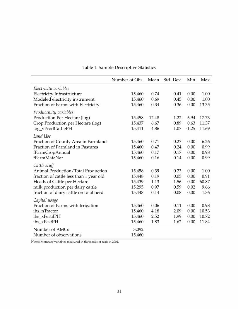
Table 1: Sample Descriptive Statistics

Number of Obs. Mean Std. Dev. Min Max

Electricity variablesElectricity Infrastructure 15,460 0.74 0.41 0.00 1.00Modeled electricity instrument 15,460 0.69 0.45 0.00 1.00Fraction of Farms with Electricity 15,460 0.34 0.36 0.00 13.35

Productivity variablesProduction Per Hectare (log) 15,458 12.48 1.22 6.94 17.73Crop Production per Hectare (log) 15,437 6.67 0.89 0.63 11.37log_vProdCattlePH 15,411 4.86 1.07 -1.25 11.69

Land UseFraction of County Area in Farmland 15,460 0.71 0.27 0.00 6.26Fraction of Farmland in Pastures 15,460 0.47 0.24 0.00 0.99fFarmCropAnnual 15,460 0.17 0.17 0.00 0.98fFarmMataNat 15,460 0.16 0.14 0.00 0.99

Cattle stuffAnimal Production/Total Production 15,458 0.39 0.23 0.00 1.00fraction of cattle less than 1 year old 15,448 0.19 0.05 0.00 0.91Heads of Cattle per Hectare 15,439 1.13 1.56 0.00 60.87milk production per dairy cattle 15,295 0.97 0.59 0.02 9.66fraction of dairy cattle on total herd 15,448 0.14 0.08 0.00 1.36

Capital usageFraction of Farms with Irrigation 15,460 0.06 0.11 0.00 0.98ihs_nTractor 15,460 4.18 2.09 0.00 10.53ihs_xFertilPH 15,460 2.52 1.99 0.00 10.72ihs_xPestPH 15,460 1.83 1.62 0.00 11.84

Number of AMCs 3,092Number of observations 15,460

Notes: Monetary variables measured in thousands of reais in 2002.

31

Table 2: First-Stage Results

Dependent Variable Electricity Infrastructure Fractions of Farmswith Electricity

(1) (2) (3) (4) (5)

Modeled electricity availability 0.326⇤⇤⇤ 0.265⇤⇤⇤ 0.264⇤⇤⇤ 0.158⇤⇤⇤[0.0422] [0.0358] [0.0359] [0.0338]

Electricity Infrastructure 0.107⇤⇤⇤[0.0187]

Year dummies Yes Yes Yes Yes Yes

Jungle ⇥ year dummies No Yes Yes Yes Yes

Water flow ⇥ year dummies No No Yes No No

River gradient ⇥ year dummies No No Yes No No

Observations 15,460 15,460 15,460 15,460 15,460Mean dep. var. 0.740 0.740 0.740 0.338 0.338F-stat 59.7 54.8 54.0 21.8 32.4p-value 0.000 0.000 0.000 0.000 0.000

Notes: In columns 1–3 the dependent variable is prevalence of electricity infrastructure in the county, measured from infrastructur in-ventories. Each colum adds controls that soak up variation from our instrument. Adding water flow and river gradient interactedwith year dummies (column 3) does not change the point estimate substatially. We therefore keep the specification in column 2 as ourpreferred specification througout the paper. In columns 4 amd 5, the dependent variable is the fraction of farms with electricity in thecounty, measured from the Censuses of Agriculture. Standard errors clustered at county level in brackets. All specifications includecounty fixed effects and use county area weights.⇤ p < 0.10, ⇤⇤ p < 0.05, ⇤⇤⇤ p < 0.01

32

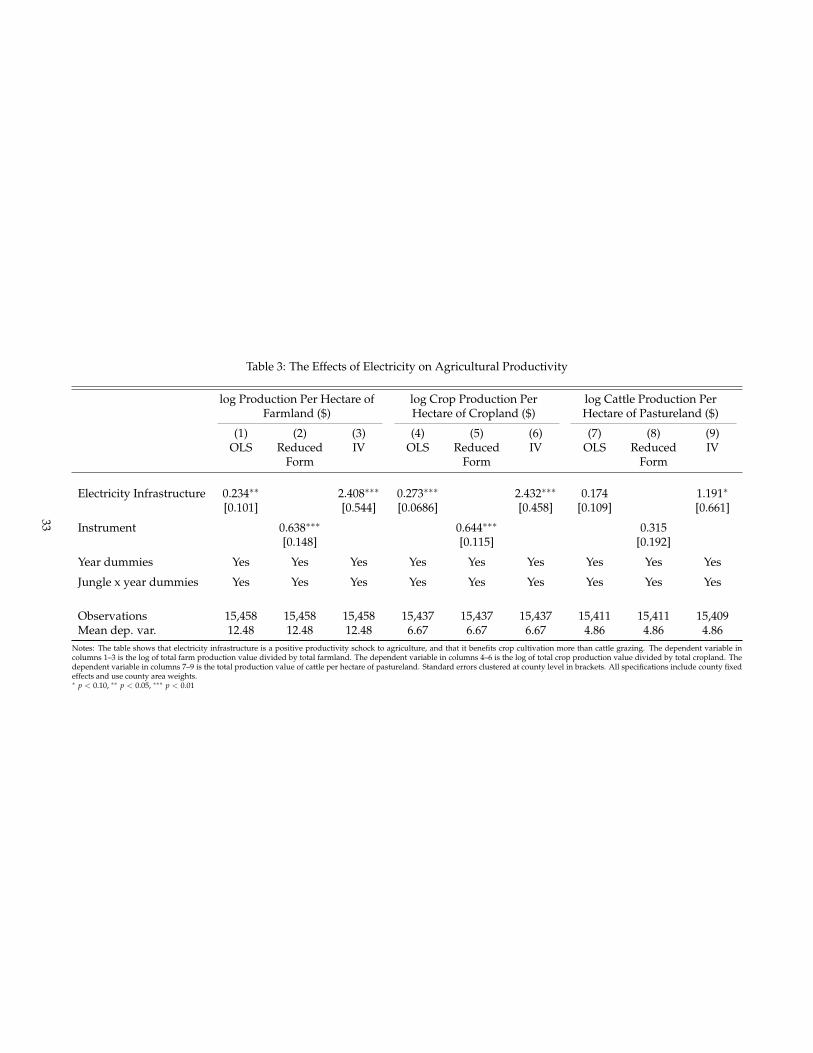
Table 3: The Effects of Electricity on Agricultural Productivity

log Production Per Hectare ofFarmland ($)

log Crop Production PerHectare of Cropland ($)

log Cattle Production PerHectare of Pastureland ($)

(1) (2) (3) (4) (5) (6) (7) (8) (9)OLS Reduced

FormIV OLS Reduced

FormIV OLS Reduced

FormIV

Electricity Infrastructure 0.234⇤⇤ 2.408⇤⇤⇤ 0.273⇤⇤⇤ 2.432⇤⇤⇤ 0.174 1.191⇤[0.101] [0.544] [0.0686] [0.458] [0.109] [0.661]

Instrument 0.638⇤⇤⇤ 0.644⇤⇤⇤ 0.315[0.148] [0.115] [0.192]

Year dummies Yes Yes Yes Yes Yes Yes Yes Yes Yes

Jungle x year dummies Yes Yes Yes Yes Yes Yes Yes Yes Yes

Observations 15,458 15,458 15,458 15,437 15,437 15,437 15,411 15,411 15,409Mean dep. var. 12.48 12.48 12.48 6.67 6.67 6.67 4.86 4.86 4.86

Notes: The table shows that electricity infrastructure is a positive productivity schock to agriculture, and that it benefits crop cultivation more than cattle grazing. The dependent variable incolumns 1–3 is the log of total farm production value divided by total farmland. The dependent variable in columns 4–6 is the log of total crop production value divided by total cropland. Thedependent variable in columns 7–9 is the total production value of cattle per hectare of pastureland. Standard errors clustered at county level in brackets. All specifications include county fixedeffects and use county area weights.⇤ p < 0.10, ⇤⇤ p < 0.05, ⇤⇤⇤ p < 0.01

33

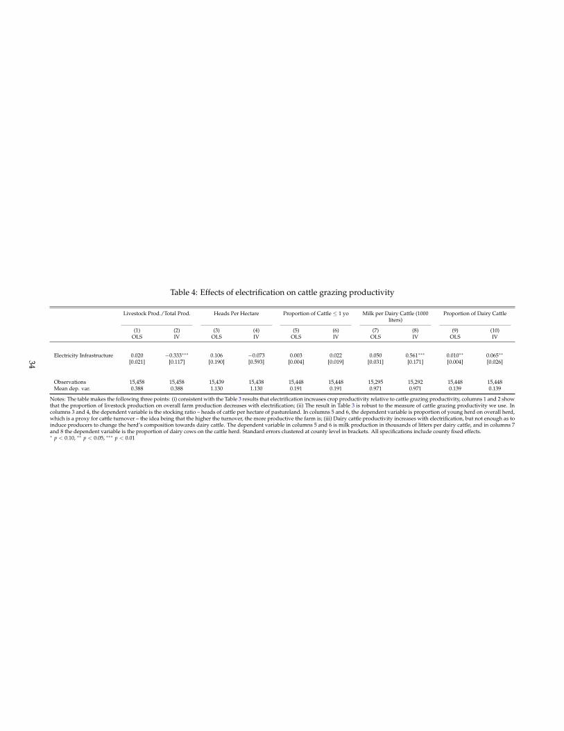
Table 4: Effects of electrification on cattle grazing productivity

Livestock Prod./Total Prod. Heads Per Hectare Proportion of Cattle 1 yo Milk per Dairy Cattle (1000liters)

Proportion of Dairy Cattle

(1) (2) (3) (4) (5) (6) (7) (8) (9) (10)OLS IV OLS IV OLS IV OLS IV OLS IV

Electricity Infrastructure 0.020 �0.333⇤⇤⇤ 0.106 �0.073 0.003 0.022 0.050 0.561⇤⇤⇤ 0.010⇤⇤ 0.065⇤⇤[0.021] [0.117] [0.190] [0.593] [0.004] [0.019] [0.031] [0.171] [0.004] [0.026]

Observations 15,458 15,458 15,439 15,438 15,448 15,448 15,295 15,292 15,448 15,448Mean dep. var. 0.388 0.388 1.130 1.130 0.191 0.191 0.971 0.971 0.139 0.139

Notes: The table makes the following three points: (i) consistent with the Table 3 results that electrification increases crop productivity relative to cattle grazing productivity, columns 1 and 2 showthat the proportion of livestock production on overall farm production decreases with electrification; (ii) The result in Table 3 is robust to the measure of cattle grazing productivity we use. Incolumns 3 and 4, the dependent variable is the stocking ratio – heads of cattle per hectare of pastureland. In columns 5 and 6, the dependent variable is proportion of young herd on overall herd,which is a proxy for cattle turnover – the idea being that the higher the turnover, the more productive the farm is; (iii) Dairy cattle productivity increases with electrification, but not enough as toinduce producers to change the herd’s composition towards dairy cattle. The dependent variable in columns 5 and 6 is milk production in thousands of litters per dairy cattle, and in columns 7and 8 the dependent variable is the proportion of dairy cows on the cattle herd. Standard errors clustered at county level in brackets. All specifications include county fixed effects.⇤ p < 0.10, ⇤⇤ p < 0.05, ⇤⇤⇤ p < 0.01

34

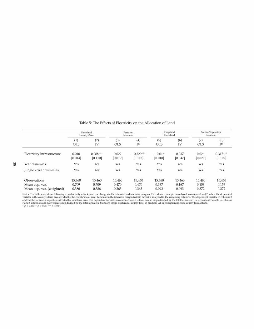
Table 5: The Effects of Electricity on the Allocation of Land

FarmlandCounty Area

PasturesFarmland

CroplandFarmland

Native VegetationFarmland

(1) (2) (3) (4) (5) (6) (7) (8)OLS IV OLS IV OLS IV OLS IV

Electricity Infrastructure 0.010 0.288⇤⇤⇤ 0.022 �0.329⇤⇤⇤ �0.016 0.037 0.024 0.317⇤⇤⇤[0.014] [0.110] [0.019] [0.112] [0.010] [0.047] [0.020] [0.109]

Year dummies Yes Yes Yes Yes Yes Yes Yes Yes

Jungle x year dummies Yes Yes Yes Yes Yes Yes Yes Yes

Observations 15,460 15,460 15,460 15,460 15,460 15,460 15,460 15,460Mean dep. var. 0.709 0.709 0.470 0.470 0.167 0.167 0.156 0.156Mean dep. var. (weighted) 0.386 0.386 0.363 0.363 0.093 0.093 0.372 0.372

Notes: The table shows how, following a productivity schock, land use changes in the extensive and intensive margins. The extensive margin is analyzed in columns 1 and 2, where the dependentvariable is the county’s farm area divided by the county’s total area. Land use in the intensive margin (within farms) is analyzed in the remaining columns. The dependent variable in columns 3and 4 is the farm area in pastures divided by total farm area. The dependent variable in columns 5 and 6 is farm area in crops divided by the total farm area. The dependent variable in columns7 and 8 is farm area in native negetation divided by the total farm area. Standard errors clustered at county level in brackets. All specifications include county fixed effects.⇤ p < 0.10, ⇤⇤ p < 0.05, ⇤⇤⇤ p < 0.01

35

Table 6: The Effects of Electricity on the Allocation of Land: Long Run

FarmlandCounty Area

PasturesFarmland

CroplandFarmland

Native VegetationFarmland

(1) (2) (3) (4) (5) (6) (7) (8)OLS IV OLS IV OLS IV OLS IV

Electricity Infrastructure �0.019 0.095 �0.006 �0.430⇤⇤⇤ �0.011 0.074 0.054⇤⇤⇤ 0.331⇤⇤⇤[0.014] [0.107] [0.020] [0.117] [0.012] [0.047] [0.021] [0.126]

Year dummies Yes Yes Yes Yes Yes Yes Yes Yes

Jungle x year dummies Yes Yes Yes Yes Yes Yes Yes Yes

Observations 12,368 12,368 12,368 12,368 12,368 12,368 12,368 12,368Mean dep. var. 0.706 0.706 0.471 0.471 0.172 0.172 0.157 0.157

Notes: This table is similar to table 5, except that the dependent variables are forward-lagged by one decade. The goal is to show that the increase in native vegetation within farms does notoccur just a short-run. The number of observations drop because we loose one period of our panel of counties. The dependent variable in columns 1 and 2 is the county’s farm area dividedby the county’s total area. The dependent variable in columns 3 and 4 is the farm area in pastures divided by total farm area. The dependent variable in columns 5 and 6 is farm area in cropsdivided by the total farm area. The dependent variable in columns 7 and 8 is farm area in native negetation divided by the total farm area. Standard errors clustered at county level in brackets.All specifications include county fixed effects.⇤ p < 0.10, ⇤⇤ p < 0.05, ⇤⇤⇤ p < 0.01

36

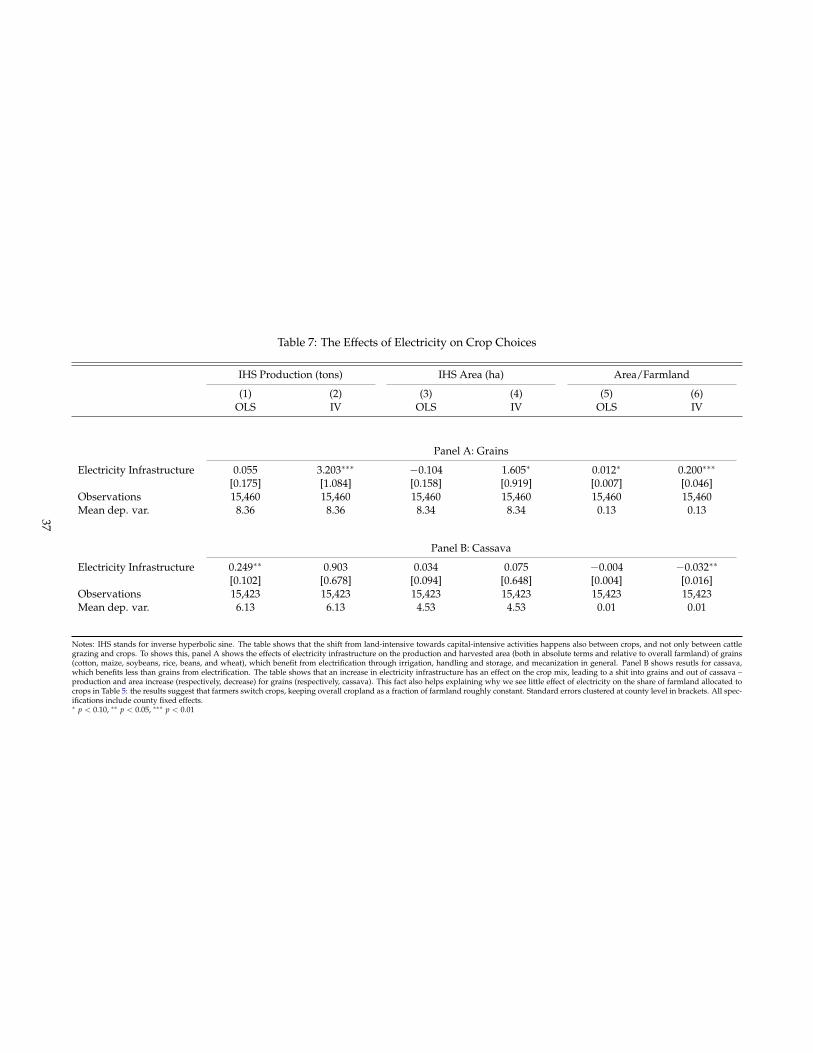
Table 7: The Effects of Electricity on Crop Choices

IHS Production (tons) IHS Area (ha) Area/Farmland

(1) (2) (3) (4) (5) (6)OLS IV OLS IV OLS IV

Panel A: Grains

Electricity Infrastructure 0.055 3.203⇤⇤⇤ �0.104 1.605⇤ 0.012⇤ 0.200⇤⇤⇤[0.175] [1.084] [0.158] [0.919] [0.007] [0.046]

Observations 15,460 15,460 15,460 15,460 15,460 15,460Mean dep. var. 8.36 8.36 8.34 8.34 0.13 0.13

Panel B: Cassava

Electricity Infrastructure 0.249⇤⇤ 0.903 0.034 0.075 �0.004 �0.032⇤⇤[0.102] [0.678] [0.094] [0.648] [0.004] [0.016]

Observations 15,423 15,423 15,423 15,423 15,423 15,423Mean dep. var. 6.13 6.13 4.53 4.53 0.01 0.01

Notes: IHS stands for inverse hyperbolic sine. The table shows that the shift from land-intensive towards capital-intensive activities happens also between crops, and not only between cattlegrazing and crops. To shows this, panel A shows the effects of electricity infrastructure on the production and harvested area (both in absolute terms and relative to overall farmland) of grains(cotton, maize, soybeans, rice, beans, and wheat), which benefit from electrification through irrigation, handling and storage, and mecanization in general. Panel B shows resutls for cassava,which benefits less than grains from electrification. The table shows that an increase in electricity infrastructure has an effect on the crop mix, leading to a shit into grains and out of cassava –production and area increase (respectively, decrease) for grains (respectively, cassava). This fact also helps explaining why we see little effect of electricity on the share of farmland allocated tocrops in Table 5: the results suggest that farmers switch crops, keeping overall cropland as a fraction of farmland roughly constant. Standard errors clustered at county level in brackets. All spec-ifications include county fixed effects.⇤ p < 0.10, ⇤⇤ p < 0.05, ⇤⇤⇤ p < 0.01

37

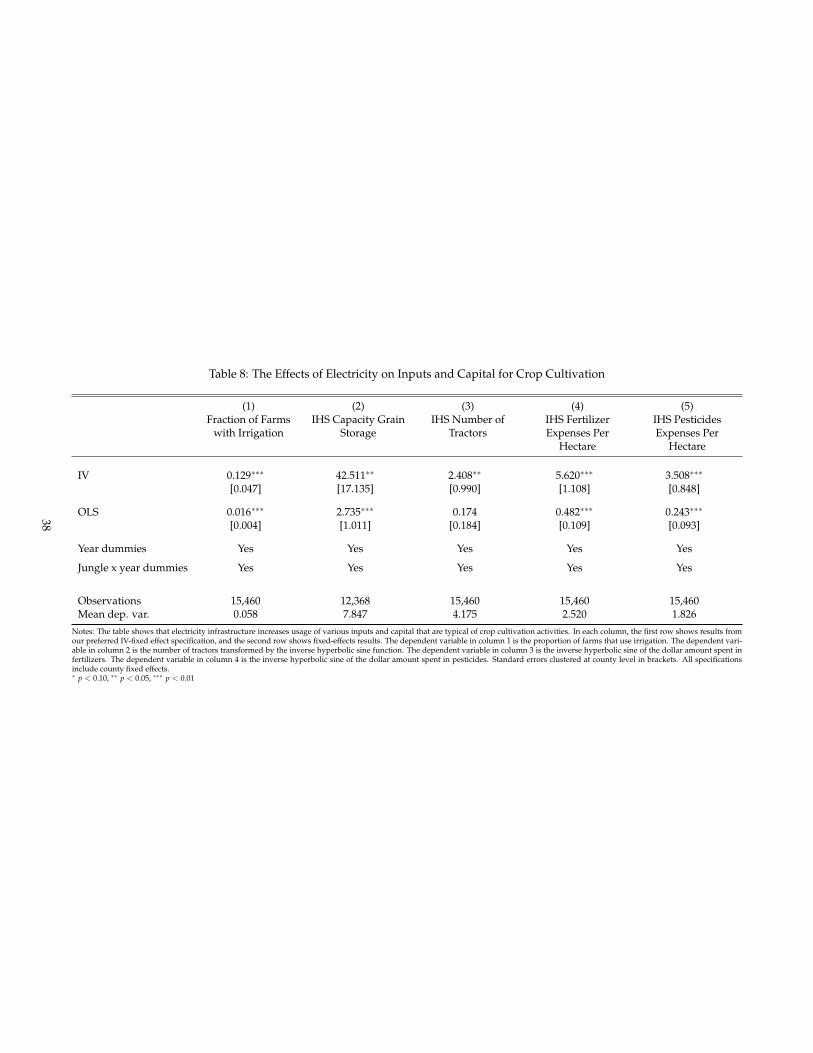
Table 8: The Effects of Electricity on Inputs and Capital for Crop Cultivation

(1) (2) (3) (4) (5)Fraction of Farms

with IrrigationIHS Capacity Grain

StorageIHS Number of

TractorsIHS FertilizerExpenses Per

Hectare

IHS PesticidesExpenses Per

Hectare

IV 0.129⇤⇤⇤ 42.511⇤⇤ 2.408⇤⇤ 5.620⇤⇤⇤ 3.508⇤⇤⇤[0.047] [17.135] [0.990] [1.108] [0.848]

OLS 0.016⇤⇤⇤ 2.735⇤⇤⇤ 0.174 0.482⇤⇤⇤ 0.243⇤⇤⇤[0.004] [1.011] [0.184] [0.109] [0.093]

Year dummies Yes Yes Yes Yes Yes

Jungle x year dummies Yes Yes Yes Yes Yes

Observations 15,460 12,368 15,460 15,460 15,460Mean dep. var. 0.058 7.847 4.175 2.520 1.826

Notes: The table shows that electricity infrastructure increases usage of various inputs and capital that are typical of crop cultivation activities. In each column, the first row shows results fromour preferred IV-fixed effect specification, and the second row shows fixed-effects results. The dependent variable in column 1 is the proportion of farms that use irrigation. The dependent vari-able in column 2 is the number of tractors transformed by the inverse hyperbolic sine function. The dependent variable in column 3 is the inverse hyperbolic sine of the dollar amount spent infertilizers. The dependent variable in column 4 is the inverse hyperbolic sine of the dollar amount spent in pesticides. Standard errors clustered at county level in brackets. All specificationsinclude county fixed effects.⇤ p < 0.10, ⇤⇤ p < 0.05, ⇤⇤⇤ p < 0.01

38

A Appendix

39

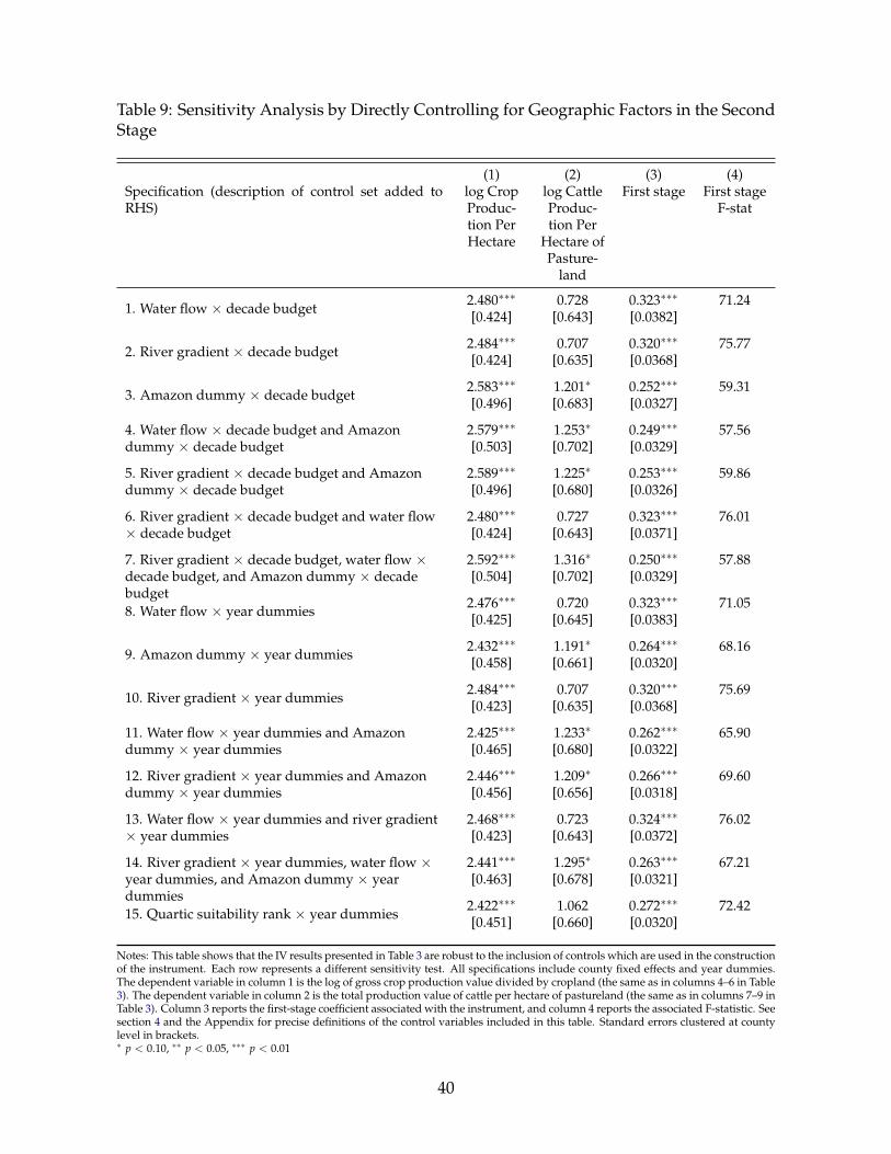
Table 9: Sensitivity Analysis by Directly Controlling for Geographic Factors in the SecondStage

(1) (2) (3) (4)Specification (description of control set added toRHS)

log CropProduc-tion PerHectare

log CattleProduc-tion Per

Hectare ofPasture-

land

First stage First stageF-stat

1. Water flow ⇥ decade budget 2.480⇤⇤⇤ 0.728 0.323⇤⇤⇤ 71.24[0.424] [0.643] [0.0382]

2. River gradient ⇥ decade budget 2.484⇤⇤⇤ 0.707 0.320⇤⇤⇤ 75.77[0.424] [0.635] [0.0368]

3. Amazon dummy ⇥ decade budget 2.583⇤⇤⇤ 1.201⇤ 0.252⇤⇤⇤ 59.31[0.496] [0.683] [0.0327]

4. Water flow ⇥ decade budget and Amazondummy ⇥ decade budget

2.579⇤⇤⇤ 1.253⇤ 0.249⇤⇤⇤ 57.56[0.503] [0.702] [0.0329]

5. River gradient ⇥ decade budget and Amazondummy ⇥ decade budget

2.589⇤⇤⇤ 1.225⇤ 0.253⇤⇤⇤ 59.86[0.496] [0.680] [0.0326]

6. River gradient ⇥ decade budget and water flow⇥ decade budget

2.480⇤⇤⇤ 0.727 0.323⇤⇤⇤ 76.01[0.424] [0.643] [0.0371]

7. River gradient ⇥ decade budget, water flow ⇥decade budget, and Amazon dummy ⇥ decadebudget

2.592⇤⇤⇤ 1.316⇤ 0.250⇤⇤⇤ 57.88[0.504] [0.702] [0.0329]

8. Water flow ⇥ year dummies 2.476⇤⇤⇤ 0.720 0.323⇤⇤⇤ 71.05[0.425] [0.645] [0.0383]

9. Amazon dummy ⇥ year dummies 2.432⇤⇤⇤ 1.191⇤ 0.264⇤⇤⇤ 68.16[0.458] [0.661] [0.0320]

10. River gradient ⇥ year dummies 2.484⇤⇤⇤ 0.707 0.320⇤⇤⇤ 75.69[0.423] [0.635] [0.0368]

11. Water flow ⇥ year dummies and Amazondummy ⇥ year dummies

2.425⇤⇤⇤ 1.233⇤ 0.262⇤⇤⇤ 65.90[0.465] [0.680] [0.0322]

12. River gradient ⇥ year dummies and Amazondummy ⇥ year dummies

2.446⇤⇤⇤ 1.209⇤ 0.266⇤⇤⇤ 69.60[0.456] [0.656] [0.0318]

13. Water flow ⇥ year dummies and river gradient⇥ year dummies

2.468⇤⇤⇤ 0.723 0.324⇤⇤⇤ 76.02[0.423] [0.643] [0.0372]

14. River gradient ⇥ year dummies, water flow ⇥year dummies, and Amazon dummy ⇥ yeardummies

2.441⇤⇤⇤ 1.295⇤ 0.263⇤⇤⇤ 67.21[0.463] [0.678] [0.0321]

15. Quartic suitability rank ⇥ year dummies 2.422⇤⇤⇤ 1.062 0.272⇤⇤⇤ 72.42[0.451] [0.660] [0.0320]

Notes: This table shows that the IV results presented in Table 3 are robust to the inclusion of controls which are used in the constructionof the instrument. Each row represents a different sensitivity test. All specifications include county fixed effects and year dummies.The dependent variable in column 1 is the log of gross crop production value divided by cropland (the same as in columns 4–6 in Table3). The dependent variable in column 2 is the total production value of cattle per hectare of pastureland (the same as in columns 7–9 inTable 3). Column 3 reports the first-stage coefficient associated with the instrument, and column 4 reports the associated F-statistic. Seesection 4 and the Appendix for precise definitions of the control variables included in this table. Standard errors clustered at countylevel in brackets.⇤ p < 0.10, ⇤⇤ p < 0.05, ⇤⇤⇤ p < 0.01

40

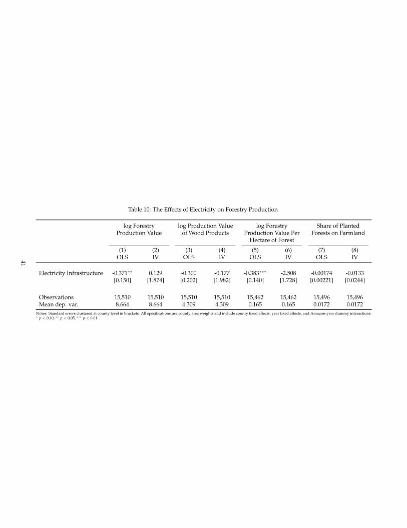
Table 10: The Effects of Electricity on Forestry Production

log ForestryProduction Value

log Production Valueof Wood Products

log ForestryProduction Value Per

Hectare of Forest

Share of PlantedForests on Farmland

(1) (2) (3) (4) (5) (6) (7) (8)OLS IV OLS IV OLS IV OLS IV

Electricity Infrastructure -0.371⇤⇤ 0.129 -0.300 -0.177 -0.383⇤⇤⇤ -2.508 -0.00174 -0.0133[0.150] [1.874] [0.202] [1.982] [0.140] [1.728] [0.00221] [0.0244]

Observations 15,510 15,510 15,510 15,510 15,462 15,462 15,496 15,496Mean dep. var. 8.664 8.664 4.309 4.309 0.165 0.165 0.0172 0.0172

Notes: Standard errors clustered at county level in brackets. All specifications use county area weights and include county fixed effects, year fixed effects, and Amazon-year dummy interactions.⇤ p < 0.10, ⇤⇤ p < 0.05, ⇤⇤⇤ p < 0.01

41

B Appendix

B.1 Model Derivation

Proposition 1. The optimal land use and production choices for farmers, H⇤c (W), H⇤

g(W), N⇤(W),satisfy equations (4)–(7) in section 3.

Proof. The solution to the farmer’s problem is given by the set of first-order conditions

wrt Hc : WNFH(H⇤c ) = (1 + l)p (13)

wrt Hg : FH(H⇤g) = (1 + l)p (14)

wrt N : WF(H⇤c ) = (1 + l)r (15)

constraint l(rN⇤ + p(H⇤c + H⇤

g)� M) = 0 (16)

where l is the Lagrange multiplier associated with equation (2).

To prove equation (4), note that equations (13) and (15) imply that N⇤ = pr

F(H⇤c )

FH(H⇤c )

and thus∂N⇤∂H⇤

c> 0.

To prove equation (5), note that combining equations (14) and (15) and taking derivativeswith respect to W gives

rp

FHH(Hg)dHg

dW� WFHH(Hc)

dHcdW

= FH(Hc) (17)

Furthermore, taking derivatives with respect to W in equation (16) and re-arranging yields

⇣1 +

rp

dNdHc

⌘dHcdW

= �dHg

dW(18)

Now, substituting (18) into (17), we can see that dHc/dW > 0:

� rp

FHH(Hg)⇣

1 +rp

dNdHc

⌘dHcdW

� WFHH(Hc)dHcdW

= FH(Hc) (19)

Electrification therefore increases the productivity of N and induces farmers to invest inmore N. N is useful for cultivation, which increases the land allocated to cultivation.This necessarily leads credit constrained farmers to lower land allocated to cattle grazing,because a larger share of their budget is spent on cultivation.

42

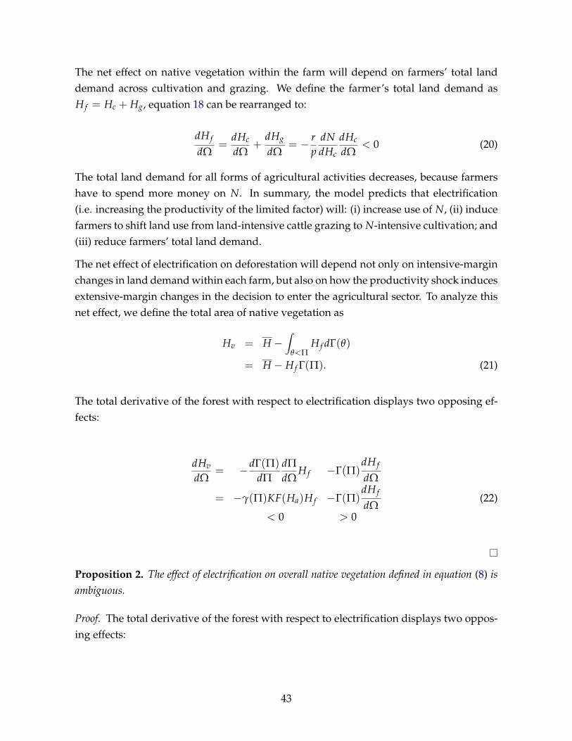
The net effect on native vegetation within the farm will depend on farmers’ total landdemand across cultivation and grazing. We define the farmer’s total land demand asHf = Hc + Hg, equation 18 can be rearranged to:

dHf

dW=

dHcdW

+dHg

dW= � r

pdNdHc

dHcdW

< 0 (20)

The total land demand for all forms of agricultural activities decreases, because farmershave to spend more money on N. In summary, the model predicts that electrification(i.e. increasing the productivity of the limited factor) will: (i) increase use of N, (ii) inducefarmers to shift land use from land-intensive cattle grazing to N-intensive cultivation; and(iii) reduce farmers’ total land demand.

The net effect of electrification on deforestation will depend not only on intensive-marginchanges in land demand within each farm, but also on how the productivity shock inducesextensive-margin changes in the decision to enter the agricultural sector. To analyze thisnet effect, we define the total area of native vegetation as

Hv = H �Z

q<PHf dG(q)

= H � Hf G(P). (21)

The total derivative of the forest with respect to electrification displays two opposing ef-fects:

dHvdW

= �dG(P)dP

dPdW

Hf �G(P)dHf

dW

= �g(P)KF(Ha)Hf �G(P)dHf

dW(22)

< 0 > 0

Proposition 2. The effect of electrification on overall native vegetation defined in equation (8) isambiguous.

Proof. The total derivative of the forest with respect to electrification displays two oppos-ing effects:

43

dHvdW

= �dHc + dHg

dWG(q)� (Hc + Hg)G(q)[

dPdW

� dq

dW] (23)

dHvdW

= �dG(P)dP

dPdW

Hf �G(P)dHf

dW

= �g(P)KF(Ha)Hf �G(P)dHf

dW(24)

< 0 > 0

References

Angelsen, A. and Kaimowitz, D., editors (2001). Agricultural Technologies and Tropical De-forestation. CABI Publiching.

BenYishay, A. and Mobarak, A. M. (2014). Social Learning and Communication. NBERWorking Papers 20139, National Bureau of Economic Research, Inc.

BRASIL (2007). Balanco energetico nacional 2007: ano base 2006. Technical Re-port 194 p, Ministerio de Minas e Energia, EPE, Rio de Janeiro. available athttps://ben.epe.gov.br/downloads/BEN2007_Versao_Completa.pdf.

Burgess, R., Hansen, M., Olken, B. A., Potapov, P., and Sieber, S. (2012). The politicaleconomy of deforestation in the tropics. The Quarterly journal of economics, 127(4):1707–1754.

Conley, T. G. and Udry, C. R. (2010). Learning about a new technology: pineapple inGhana. American Economic Review, 100(1):35–69.

Conning, J. and Udry, C. (2007). Rural Financial Markets in Developing Countries, volume 3of Handbook of Agricultural Economics, chapter 56, pages 2857–2908. Elsevier.

Cropper, M., Griffiths, C., and Jyotsna (2001). Predicting Spatial Patterns of Deforestation:The Role of Roads and Protected Areas in North Thailand. Land Economics, May.

Cropper, M., Griffiths, C., and Mani, M. (1999). Roads, Population Pressures, and Defor-estation in Thailand, 1976-1989. Land Economics, 75 (1):58–73.

44

Dinkelman, T. (2011). The Effects of Rural Electrification on Employment: New Evidencefrom South Africa. American Economic Review, 101(7):3078–3108.

Donaldson, D. (forthcoming). Railroads of the raj: Estimating the impact of transportationinfrastructure. American Economic Review.

Duflo, E. and Pande, R. (2007). Dams. The Quarterly Journal of Economics, 122(2):pp. 601–646.

Dyson, T. (1996). Population and Food: Global Trends and Future Prospects. Routledge.

Foster, A. D. and Rosenzweig, M. R. (2003). Economic growth and the rise of forests. TheQuarterly Journal of Economics, 118(2):pp. 601–637.

Grossman, G. M. and Krueger, A. B. (1991). Environmental impacts of a north americanfree trade agreement. National Bureau of Economic Research Working Paper 3914, NBER,Cambridge MA.

Grossman, G. M. and Krueger, A. B. (1995). Economic growth and the environment. Quar-terly Journal of Economics, 110:353–377.

Hornbeck, R. and Keskin, P. (2014). The historically evolving impact of the ogallalaaquifer: Agricultural adaptation to groundwater and drought. American Economic Jour-nal: Applied Economics, 6(1):190–219.

Jayachandran, S., de Laat, J., Lambin, E. F., and Stanton, C. Y. (2016). Cash for carbon: Arandomized controlled trial of payments for ecosystem services to reduce deforestation.Working Paper 22378, National Bureau of Economic Research.

Jill L. Caviglia-Harris, Dustin Chambers, J. R. K. b. (2009). Taking the “u” out of kuznets: Acomprehensive analysis of the ekc and environmental degradation. Ecological Economics,(68):1149–1159.

Lewis, J. and Severnini, E. (2015). The value of rural electricity: Evidence from the rolloutof the us power grid. Technical report, Mimeo.

Lipscomb, M., Mobarak, A. M., and Barham, T. (2013). Development Effects of Electri-fication: Evidence from the Topographic Placement of Hydropower Plants in Brazil.American Economic Journal: Applied Economics, 5(2):200–231.

Pfaff, A. (1999). What Drives Deforestation in the Brazilian Amazon? Evidence fromSatellite and Socioeconomic Data. Journal of Environmental Economics and Management,37(1):26–43.

45

Porras, I. (2012). Payments for environmental services in costa rica: from rio to rio andbeyond. iied Briefing.

Rud, J. P. (2012). Electricity provision and industrial development: Evidence from india.Journal of Development Economics, 97:352–367.

Sekhri, S. (2011). Public provision and protection of natural resources: Groundwater irri-gation in rural india. Amercian Economic Journal: Applied Economics, 3(4):29–55.

Stavins, R. N. and Jaffe, A. B. (1990). Unintended Impacts of Public Investments on PrivateDecisions: The Depletion of Forested Wetlands. The American Economic Review, 80(3):pp.337–352.

Stern, D. I. (2004). The rise and fall of the environmental kuznets curve. World Development,32(8):1419–1439.

Stern, N. (2008). The economics of climate change. American Economic Review, 98(2):1–37.

World Bank (1990). Brazil - irrigation subsector review. Sector Report 7797, World Bank.

Zomer, R. J., Trabucco, A., Coe, R., and Place, F. (2014). Trees on farms: an update and re-analysis of agroforestry’s global extent and socio-ecological characteristics. World Agro-forestry Center Working Paper 179.

46