agricultural production, dietary diversity, and climate

Policy Research Working Paper 7022

Agricultural Production, Dietary Diversity, and Climate Variability

Andrew DillonKevin McGee

Gbemisola Oseni

Development Research GroupPoverty and Inequality TeamSeptember 2014

WPS7022P

ublic

Dis

clos

ure

Aut

horiz

edP

ublic

Dis

clos

ure

Aut

horiz

edP

ublic

Dis

clos

ure

Aut

horiz

edP

ublic

Dis

clos

ure

Aut

horiz

ed

Produced by the Research Support Team

Abstract

The Policy Research Working Paper Series disseminates the findings of work in progress to encourage the exchange of ideas about development issues. An objective of the series is to get the findings out quickly, even if the presentations are less than fully polished. The papers carry the names of the authors and should be cited accordingly. The findings, interpretations, and conclusions expressed in this paper are entirely those of the authors. They do not necessarily represent the views of the International Bank for Reconstruction and Development/World Bank and its affiliated organizations, or those of the Executive Directors of the World Bank or the governments they represent.

Policy Research Working Paper 7022

This paper is a product of the Poverty and Inequality Team, Development Research Group. It is part of a larger effort by the World Bank to provide open access to its research and make a contribution to development policy discussions around the world. Policy Research Working Papers are also posted on the Web at http://econ.worldbank.org. The authors may be contacted at [email protected].

Nonseparable household models outline the links between agricultural production and household consumption, yet empirical extensions to investigate the effect of produc-tion on dietary diversity and diet composition are limited. Although a significant literature has investigated the calorie-income elasticity abstracting from production, this paper provides an empirical application of the nonseparable household model linking the effect of exogenous variation in planting season production decisions via climate vari-ability on household dietary diversity. Using exogenous variation in degree days, rainfall, and agricultural capital stocks as instruments, the effect of production on house-hold dietary diversity at harvest is estimated. The empirical specifications estimate production effects on dietary diver-sity using both agricultural revenue and crop production

diversity. Significant effects of agricultural revenue and crop production diversity on dietary diversity are estimated. The dietary diversity-production elasticities imply that a 10 per-cent increase in agricultural revenue or crop diversity results in a 1.8 percent or 2.4 percent increase in dietary diversity, respectively. These results illustrate that agricultural income growth or increased crop diversity may not be sufficient to ensure improved dietary diversity. Increases in agricul-tural revenue do change diet composition. Estimates of the effect of agricultural income on share of calories by food groups indicate relatively large changes in diet composition. On average, a 10 percent increase in agricultural revenue makes households 7.2 percent more likely to consume vegetables and 3.5 percent more likely to consume fish, and increases the share of tubers consumed by 5.2 percent.

Agricultural Production, Dietary Diversity, and Climate Variability

Andrew Dillon Michigan State University

Kevin McGee

American University

Gbemisola Oseni World Bank

Keywords: Agriculture, Crop Diversity, Dietary Diversity, Nutrition, Rainfall, Temperature JEL Codes: Q12, O13 __________________________________ Acknowledgements: We appreciate the helpful comments of Gero Carletto, Alan de Brauw, John Maluccio, Paul Winters, an anonymous referee, and the participants of the Farm Household Production and Nutrition conference at the World Bank. The management of the Nigeria LSMS-ISA data collection process in Nigeria benefited from the collaboration of Gero Carletto, Kinnon Scott, the Nigerian Bureau of Statistics staff, and Colin Williams. Siobhan Murray provided invaluable support to organize the GIS and climate data. All errors are our own.

I. Introduction Nonseparable household models outline the links between agricultural production and

household consumption, yet empirical extensions to investigate the effect of production on

nutrition are limited. An early, related literature investigated the calorie-income elasticity as

part of a larger debate on whether households could grow their way out of poverty and

malnutrition, but abstracted from agricultural production (see Strauss and Thomas, 1995 for a

review). In current discussions about the role of agriculture in promoting nutrition, increased

agricultural income and increased production of nutrient rich food, especially among

subsistence farmers, are two of the pathways through which agriculture might promote

nutrition (Hoddinott 2011). However, similar to the earlier calorie-income elasticity debates,

we know little about whether agricultural income growth or production diversity is likely to

have a larger effect on dietary diversity and diet composition. This paper provides an

empirical application of the nonseparable household model to identify the effect of variation

in planting season production via exogenous climate variability on household dietary diversity

and diet composition.

Household dietary diversity is strongly associated with household calorie availability (Ruel

2003), an important component of nutritional status, while diet composition is associated with

the consumption of particular micronutrients as well as diet quality. However, it should be

noted that household nutrition measures fundamentally proxy for individual level food

intakes. Intrahousehold distribution of calories and micronutrients is unlikely to be uniform

across household members. Despite this important caveat, dietary diversity and diet

composition are important nutritional indicators in rural subsistence populations (Ruel 2003,

2

Swindale and Bilinsky 2006, FAO 2011). Dietary diversity is one method of measuring data

quality. The paper also uses the components of the household dietary diversity score to

measure the effect of increased production on the share of total calories by food group.

Using recent panel data from Nigeria that includes observations from both planting and

harvest seasons within an agricultural season, our econometric strategy uses degree day and

rainfall deviations from historical means as well as agricultural input prices and quasi-fixed

agricultural capital to instrument for production variables (agricultural revenue or crop

production diversity) which are simultaneously determined with consumption. Degree days, a

cumulative measure of optimal temperatures for plant growth, have been found to be

correlated with reduced yields and agricultural income (Hatfield et al. 2008). We identify the

effect of revenue variation on dietary diversity and diet composition in an empirical

application of the nonseparable household model by using exogenous variation in rainfall and

degree days that affect plant growth and agricultural revenue, but do not necessarily change

market level prices at harvest which affect consumption patterns. This mechanism through

which the exclusion restriction assumption could be violated can be tested in our data.

A small literature has investigated the effects of agricultural production on nutrition primarily

via reduced form identification strategies. Muller (2009) found that production of food crops

such as beans and certain tubers as well as a category composed of heterogeneous food of

high quality had positive impacts on nutritional statuses, while the production of traditional

beers and nonfood crops was found to have negative effects for nutrition. The authors also

found production of other fruits and vegetables was associated with better health status.

3

Although agriculture is primarily a rural activity in many developing nations, there has also

been evidence that urban agricultural production has positive effects on nutrition. In their

study of 15 developing countries, Zezza and Tasciotti (2010) find that urban agriculture does

appear to be associated with greater dietary diversity and calorie availability after controlling

for economic welfare and a set of household characteristics. Using a smaller set of countries

Zezza and Tasciotti (2010) also find some evidence of a relationship between participation in

urban agriculture and greater calorie consumption. Fruits and vegetables were the food

groups more consistently found to contribute to the increase in calorie consumption.

Fewer studies have looked at both the linkage between income and nutrition and that between

the diversity of crops produced and nutrition. Food prices, access to markets and credit can

influence decisions on what type of crops households grow. For example, smallholder farmers

are more likely to grow food crops to ensure food self-sufficiency rather that grow cash crops

and thus staple food expenditures have low income elasticity (Fafchamps, 1992). Using a

nationally representative household survey of India, Bhagowalia et al. (2012) examine the

relationship between agricultural income and nutrition (measured using children’s

anthropometric indicators), as well as agricultural production. They find a modest effect of

income on nutritional status unless accompanied by improved health and education outcomes.

However, they also find strong evidence that agricultural production conditions such as

irrigation, crop diversity and ownership of livestock, substantially influence household dietary

diversity. Jones et al. (2014) also find a strong positive association between production

diversity and household dietary diversity in Malawi.

4

There have been even fewer studies using data from Nigeria to examine the agriculture and

nutrition linkage and the few papers that do exist are case studies or only use descriptive

statistics (Babatunde et al., 2010; Okezie and Nwosu, 2007). Babatunde et al. (2010)

examines the relationship between income and calorie intake for farm households in rural

Nigeria using household data from 40 villages in Kwara state. Although, the authors find a

significant positive relationship between income and calorie intake, the calorie-income

elasticity was estimated as 0.181 suggesting that calorie intake does not increase substantially

with income. They also find a positive relationship between farm size and calorie intake in

Nigeria. Okezie and Nwosu (2007) examined the effect of agricultural commercialization on

nutritional status of children in Abia state in Nigeria and found that children in households

that are more commercialized recorded a higher prevalence of underweight and stunting.

Given the existing gaps in the literature, the present study contributes to the literature by using

nationally representative data from Nigeria that contains information on household

consumption, agricultural production, and geospatial variables to examine the link between

agriculture production and dietary diversity. The econometric strategy of the paper is based on

the nonseparable household literature to estimate the causal effects of production diversity on

dietary diversity rather than associations. In previous cross-sectional studies, identification of

the income and nutrition interlinkage may be confounded by the inability to distinguish the

causal direction of the interlinkage, as higher income households may have increased

nutrition, but households with better nutrition may also have higher productivity and higher

incomes. By modeling this causal relationship using a nonseparable household model and

using exogenous variation in degree days and rainfall and agricultural capital as instruments,

5

the casual direction of the production-dietary diversity relationship is more clearly identified.

The empirical estimates suggest significant effects of both agricultural revenue and crop

production diversity on dietary diversity. A revenue-dietary diversity elasticity of 0.18 and a

crop diversity-dietary diversity elasticity of 0.24 were estimated. We have most confidence in

the revenue-dietary diversity estimates as this specification clearly passes all instrumental

variable tests. Climate variability is also shown to have differing effects on revenue versus

crop production diversity. Deviations from historical means of both rainfall and degree days

has statistically significant effects on agricultural revenue while only deviations from rainfall

means have statistically significant effects on crop production diversity.

The investigation below also reveals differential impacts of production variability on the

likelihood of food group consumption and the share of calories consumed from separate food

groups. A 10% increase of agricultural revenue increases the likelihood of a household

reporting consumption of vegetables by 7.2% and fish by 3.5%. Increased agricultural revenue

is found to induce households to alter the composition of their diets by lowering the share of

consumption from beverages and increasing tuber consumption shares. A 10% increase in

agricultural revenue results in a decrease in the consumption share of beverages by 5.9% but

increases the consumption share of tubers by 5.2%. Estimates of changes in other food groups

were either not statistically significant or did not pass all instrumental variables tests.

In the next section of the paper, the data is described including the construction of the climate

variability and degree day variables. The third section outlines the econometric strategy of the

paper, while the fourth section presents the paper’s key results. The last section concludes.

6

II. Data Description This study uses data from Wave 1 of the General Household Survey-Panel (GHS-Panel)

conducted in 2010/11 by the Nigeria National Bureau of Statistics (NBS) in collaboration with

the World Bank Living Standard Measurement Study - Integrated Surveys on Agriculture

(LSMS-ISA) project. The GHS-Panel survey is modeled after the Living Standard Measurement

Study (LSMS) surveys and is representative at the national, zonal, and rural/urban levels. The

total sample consists of about 5,000 households covering all 36 states in the country and the

Federal Capital Territory, Abuja. One of the main objectives of the GHS-Panel is to improve

agriculture data collection in Nigeria by collecting information at disaggregated levels (crop,

plot, and household levels), and linking such data to nonagricultural aspects of livelihoods. All

households were visited at two points in time: right after planting (post planting visit) and right

after harvest (post-harvest visit) and were administered multi-topic household, agriculture and

community questionnaires. Amongst a variety of topics, the household questionnaire gathered

detailed information on food and nonfood consumption and expenditure of households. The

survey covers over 100 food items commonly consumed in Nigeria and collected information on

household consumption (quantity consumed) of the items in the past seven days before the

survey. The use of handheld GPS devices to record coordinates of household plots allows the

linkage of the data with geospatial variables such as rainfall and temperature data from other

sources. Of the 5,000 households in the survey, about 3,000 were agricultural households in rural

and urban areas producing a wide variety of crops. The study focuses on the rural agricultural

households interviewed for the GHS-Panel 2010/11 survey and all statistics are weighted to

ensure representativeness at national, regional and rural/urban levels.

7

Using the consumption data from the GHS-Panel, dietary diversity indicators from the harvest

round of the data are constructed. The indicator is constructed by classifying food items from the

consumption module into 12 distinct food groups. The food groups are delineated according to

guidelines from the Food and Agriculture Organization (Kennedy et al, 2011). Dietary diversity

is an important nutritional indicator of household calorie availability. In a review of the

nutritional literature on validation studies, Ruel (2003) documents a consistent set of results in

developing countries which illustrate this positive correlation between dietary diversity measures

and nutrient adequacy. For this reason, the present study uses household dietary diversity as its

primary nutritional measure. In addition to dietary diversity, calorie intake from food groups is

included in the descriptive analysis. Calorie intake and production was estimated using the

consumption and agricultural production data in the GHS-Panel and applying calorie conversions

for each item from the U.S. Department of Agriculture's National Nutrient Database for Standard

Reference1. The item level calorie estimates were then aggregated to the food/crop group and

household levels for use in the analysis.

The two measures of production variability used in the analysis that follows are a count of the

number of crop groups harvested and the value of agricultural output (agricultural revenue). Both

measures are calculated using information from the post-harvest round of the GHS-Panel. To

construct the count of harvested crop groups, food crops were separated into 5 groups that

correspond to 5 of the 15 groups that comprise the dietary diversity measure. Harvested nonfood

crops were excluded. Agricultural revenue was calculated using farmer estimates of the total

harvest value for each crop.

8

A major factor that could influence income (revenue) from production diversity is climate

variability. The extensive literature on climate variability and agricultural production has

established a strong relationship between climate and crop yields (Tao et al. 2009; Rowhani et

al., 2011). Rowhani et al. (2011) examined the relationship between seasonal climate and crop

yields in Tanzania and found that both intra and inter seasonal changes in temperature and

precipitation influence cereal (maize, sorghum and rice) yields in Tanzania. They found that

seasonal temperature increases have the most important impact on yields. Tao et al (2009)

found that major crop yields were significantly related to growing season climate in the main

production regions of China, and that growing season temperature had a generally significant

warming trend. Using a panel dataset, Schlenker and Lobell (2010) examine the impact of

changes in temperature and precipitation on crop yields of five main staple crops (maize,

sorghum, millet, groundnuts and cassava) in sub-Saharan Africa and find that temperature

changes have a much stronger impact on yields than precipitation changes2. Hatfield et al.

(2008) establish that degree days, the number of days extreme temperatures affect optimal

plant growth, have been found to be correlated with reduced yields and agricultural income.

For this reason, the paper uses degree day and rainfall deviations as a source of exogenous

variation in agricultural production. Daily temperature data from 1981-2010 and daily rainfall

data from 2000-2010 was extrapolated from the Surface Meteorology and Solar Energy

version 6.0 developed by the Atmospheric Sciences Data Center at NASA3 and georeferenced

to the GHS-Panel. Historical averages for the number of degree days (1981-2009) and rainfall

(2000-2009) during the planting season (April-June) were calculated for each household. The

deviations from historical planting season degree day and rainfall averages were then

calculated for the 2010 planting season.

9

In the next section, the econometric strategy for the paper is described, building on the

socioeconomic, georeferenced climate data, and dietary diversity indicators.

III. Econometric Strategy

In a nonseparable household model, production and consumption decisions are jointly

determined (Strauss 1984, Benjamin 1992, Bardhan and Udry 1999, LaFave and Thomas 2013).

Identification of the direction of causality is potentially confounded by cross sectional

correlation. In our empirical strategy, a reduced form regression of climate variables on dietary

diversity would also be mis-specified due to omitted production variables. Behrman et al. (1997)

addressed these econometric challenges by developing a dynamic nonseparable household model

which motivated using planting and harvest season data to improve the identification of calorie-

income elasticity estimates. Our strategy builds on this approach and the post-planting and post-

harvest data structure of the Nigeria LSMS-ISA by distinguishing between the timing of seasonal

production decisions to understand the effect of planting period production decisions on post-

harvest dietary diversity within a full agricultural season, t.

In the dynamic formulation of the agricultural household model, households maximize expected

utility given the production function (𝑄𝑡), time endowment (𝐸𝐿) and intertemporal budget

constraint (equation 4) (LaFave and Thomas 2013). The household’s problem is to choose

produced agricultural goods (𝑥𝑎𝑡), purchased market goods (𝑥𝑚𝑡), agricultural inputs (𝑉𝑡) and

leisure (𝑙𝑡) to maximize utility given observed (𝜇𝑡) and unobserved household characteristics (𝜀𝑡)

such that:

10

max 𝐸[∑ 𝛽𝑡𝑢(𝑥𝑎𝑡𝑥𝑚𝑡,∞𝑡=0 𝑙𝑡; 𝜇𝑡, 𝜀𝑡)] (1)

subject to the constraints :

𝑄𝑡 = 𝑄𝑡(𝐿𝑡,𝑉𝑡,𝐴𝑡;𝜃) (2)

𝐸𝐿 = 𝑙𝑡 + 𝐿𝑡𝐹 + 𝐿𝑡𝑂 (3)

𝑊𝑡+1 = (1 + 𝑟𝑡+1)[𝑊𝑡 + 𝑤𝑡(𝐸𝐿 − 𝑙𝑡) + 𝜋 − 𝑝𝑎𝑡𝑥𝑎𝑡 − 𝑝𝑚𝑡𝑥𝑚𝑡] (4)

where 𝜋𝑡 = 𝑝𝑎𝑡𝑄𝑡(𝐿𝑡,𝑉𝑡,𝐴𝑡; 𝜃) − 𝑤𝑡𝐿𝑡 − 𝑝𝑉𝑡𝑉𝑡 − 𝑝𝐴𝐴𝑡 is the profit function over season t.

Equation 2 represents the production function which depends on vectors of farm labor (𝐿𝑡),

variable inputs (𝑉𝑡), fixed assets (𝐴𝑡) such as land and capital, and seasonal climate variability

(𝜃). The household’s time endowment (equation 3) is divided between leisure, on-farm (𝐿𝑡𝐹) and

off-farm labor (𝐿𝑡𝑂). A standard dynamic household budget constraint is represented in equation

4.

In a separable household model, demand for consumption of good c in period t is:

𝑥𝑐𝑡 = 𝑥𝑐𝑡(𝑝𝑚𝑣,𝑝𝑎𝑣,𝑤𝑣, 𝑟𝑡+1,𝜋𝑡(𝑝𝑣𝑉,𝑝𝑎𝑉 ,𝑝𝑉,𝑝𝐴𝑡;𝜃 ),𝑦𝑉, 𝜆𝑉; 𝜇𝑡, 𝜀𝑡) (5)

where good c consumption depends on market (𝑝𝑚𝑣) and agricultural prices (𝑝𝑎𝑣), the price of

variable inputs (𝑝𝑣) such as agricultural labor, fertilizer, pesticides or herbicides, interest rates

(𝑟𝑡+1), farm profits (𝜋𝑡) conditional on climate variability (𝜃), exogenous income (𝑦𝑉) and future

prices via the marginal utility of wealth (𝜆𝑉). Consumption also depends on observed (size and

composition) and unobservable household characteristics (food preferences). The problem can

be disaggregated into a recursive two-period problem where the household first maximizes

profits and then chooses consumption levels if we assume separability (Strauss et al. 1986,

Bardhan and Udry (1999)).

11

In our nonseparable formulation, production factors such as input prices influence the

household’s consumption choices such that:

𝑥𝑐𝑡 = 𝑥𝑐𝑡(𝑝𝑚𝑣,𝑝𝑎𝑣,𝑤𝑣, 𝑟𝑡+1,𝜋𝑡(𝑝𝑣𝑉,𝑝𝑎𝑉 ,𝑝𝑉,𝑝𝐴;𝜃 ),𝑝𝑣𝑉,𝑝𝑎𝑉,𝑝𝑉, 𝑝𝐴,𝑦𝑉 , 𝜆𝑉; 𝜇𝑡, 𝜀𝑡) (5)

The identification strategy to disentangle the joint production and consumption decision by the

household is to model the production-climate variability relationship as a first stage regression

controlling for other production variables including labor availability and agricultural capital

while also controlling for prices and including state level fixed effects. The state fixed effects

control for potentially omitted variables that are unobserved in our data set including interest rate

and price expectations which we assume are similar across rural areas within states. In the

second stage, exogenous climate deviations from long term means provide identification for the

effect of agricultural production variables (agricultural revenue and crop diversity) on dietary

diversity. The demand for a consumption good is generalizable to a dietary diversity indicator or

a share of calories consumed by food group after converting food quantities into calories.

More precisely, the first stage relationship between production which (Y) is determined by input

prices (𝑝𝑣), the value of agricultural capital (𝑝𝐴), climate variability (𝜃ℎ𝑠), and household

characteristics including household size and composition (X):

ln𝑌ℎ𝑣𝑠 = 𝛽𝑝𝑣𝑝𝑣 + 𝛽𝐴𝑝𝐴 + 𝛽𝜃𝜃ℎ𝑣𝑠 + 𝛽𝑥𝑋ℎ𝑣𝑠 + 𝜆𝑠 + 𝜀ℎ𝑣𝑠 (6)

In our empirical analysis, the relationship between production and climate variability includes

the specification of 𝑌ℎ𝑠 as either a crop group count index in a first set of regressions or

agricultural revenue4 in a second set of regressions. Farm capital is a quasi-fixed stock over the

12

agricultural season considered in the analysis. The motivation for including agricultural capital

is clear from the agricultural production function: agricultural capital, along with inputs, is

posited to directly affect production and hence agricultural revenue. As agricultural capital is a

stock, we argue that this stock does not change within season, though it may change across

season5. Agricultural capital likely satisfies the exclusion restriction because investments in

capital occur before post-harvest consumption measurement and unlikely to be correlated with

post-harvest consumption. The value of agricultural capital is uniformly low in our sample,

while consumption diversity is more variable. In direct tests, we find that agricultural capital is

not strongly correlated with current period consumption. Climate variables including the degree

day and rainfall deviations from historical trends are included in the above first stage equation.

State fixed effects (𝜆) are also included in this regression to control for agricultural market

integration that may affect either access to inputs or marketing opportunities for farmers.

The second stage equation establishes the relationship between production and dietary diversity

at the household level and is given by:

ln𝑁ℎ𝑣𝑠 = 𝛽𝑌 ln𝑌ℎ𝑣𝑠 + 𝛽𝑝𝑚𝑝𝑚 + 𝛽𝑝𝑣𝑝𝑣 + 𝛽𝑥𝑋𝑣ℎ𝑠 + 𝜆𝑠 + 𝜀ℎ𝑣𝑠 (7)

where 𝑁ℎ𝑠 is dietary diversity for household h in village v in state s. Dietary diversity is

determined by agricultural production Y, market prices (𝑝𝑚) during the post-harvest period,

variable input prices (𝑝𝑣), and household characteristics X including household composition

which may affect household consumption. Y is endogenously determined so we instrument with

local climate variables and agricultural capital which are correlated with production variables,

but uncorrelated with dietary diversity. The plausibility of the excludability condition depends

on the spatial intensity of climate shocks and market integration. While climate shocks could

13

have an effect on dietary diversity via price variation, the econometric specification includes

market prices in the second stage. Further, rural Nigerian markets seem to be sufficiently

integrated that local climate variability causes reduction in yields for local farmers, but these

climate induced yield variations have small effects on equilibrium prices. Hence, the pathway

through which climate variation affects dietary diversity is through the quantity of crops

available for the household’s own-consumption or in our second specification through the

agricultural income generated from production, but not via local climate variability induced price

changes.

Testing the Exclusion Restriction

The validity of the exclusion restriction potentially invalidates the identification of the effect of

production variables on the nutritional outcomes. The primary concern is that climate variation

may be correlated with dietary diversity or calorie shares by food group. This would be the case

if climate variation produced general equilibrium price changes that in turn affect consumption

through market prices independently of their effect on production.

One approach to test this mechanism and find evidence that the exclusion restriction is indeed

invalid would be to estimate the effect of climate directly on market level prices. Any potential

general equilibrium effects of climate variation on market prices, either through deviation from

historical averages of degree days or rainfall, can be estimated directly. As a test of one potential

mechanism that would violate the exclusion restriction, the climate-price specification is

estimated at the enumeration area level, the unit of analysis that most closely correlates to local

14

markets in our data. If strong correlations exist between the climate shocks and market prices,

the exclusion restriction would be clearly violated.

IV. Results Tables 1-4 examine the descriptive linkages between production, climate, and nutrition. In

Tables 1-3, households are separated into degree day and rainfall deviation quartiles where

deviations are with respect to the historical mean of the climate variable. Those households in

the first quartile experienced larger negative deviations (e.g. below average rainfall, fewer degree

days) while those in the fourth experienced larger positive deviations (e.g. higher rainfall and

more degree days). Increased degree days have negative effects on crop yields and agricultural

income for a variety of crops (Hatfield et al. (2008), Schlenker and Lobell (2010)).

Table 1 provides descriptive estimates for total production across degree day and rainfall shock

quartiles. For both degree day and rainfall shocks, an inverted-U relationship is observed

whereby agricultural revenue is highest when there is a small deviation from average weather but

smallest when there are large positive or negative shocks. Negative rainfall shocks and positive

degree day shocks appear to have the greatest effect on agricultural revenue. Table 1 suggests

there is a strong relationship between degree day and rainfall variability and the type of crops

harvested by the household. Grains and flours as well as pulses, nuts, and seeds were more likely

to be harvested by households that experienced above average temperatures (degree days) and

below average rainfall during the planting season. This may be because grains and pulses are

generally more drought and heat tolerant than other crops. For all other crop groups, the reverse

descriptive trend is observed. The middle panels of Table 1 present the shares of total

production in terms of both agricultural revenue and the calories produced of each crop group.

15

Variations in the production shares across the climate shock quartiles are nearly identical to those

for the production indicators in the top panel.

Table 2 examines the descriptive relationship between crop diversity and climate deviations. In

contrast to agricultural revenue, the number of crop groups harvested exhibits a weakly positive

relationship with degree day shocks and a weakly negative relationship with rainfall shocks.

Positive rainfall deviations potentially reduce production uncertainty in the early planting period

which results in less need to diversify planting. Increased degree days imply higher temperatures

during the agricultural season and increased production uncertainty which may increase farmer’s

crop diversification. The bottom panel of Table 2 presents the share of cultivated land devoted

to each crop group. In general, the land shares follow the same pattern as production shares in

Table 1. Overall, the descriptive results highlight an important linkage between climate

variability and agricultural production.

The relationship between climate variations and both dietary diversity and food group

consumption is explored in Table 3. The estimates in the top panel suggest that wetter weather is

associated with higher dietary diversity. Rainfall conditions that are more favorable to

agricultural production are associated with improved dietary diversity, while there is a negative

association between degree day shocks and dietary diversity. The middle panel of Table 3

presents calorie consumption shares of each food group. Variations across climate shock

quintiles are similar to the production patterns shown in Table 1. The consumption share of

grains and flours as well as pulses, nuts, and seeds is higher on average in households that

experience above average temperatures and below average rainfall while the opposite is largely

16

true for all remaining categories. A similar pattern is found in the bottom panel of Table 3 where

the calorie consumption share from own production is presented.

Table 4 examines the relationship between agricultural revenue and dietary diversity. The

estimates in the top panel of Table 4 do not suggest a clear trend between the number of food

groups consumed and agricultural revenue. Curiously, households with the lowest agricultural

revenue consumed the most food groups on average. These may be the farmers who consume

entirely out of own production. Further, wealthier rural households may engage in agriculture as

a side activity with a nonfarm activity as their main source of income. Such households will

probably fall in the lower agricultural revenue quartile but have sufficient means to acquire a

wider variety of food. The bottom panel of the table looks at the distribution of the number of

food groups consumed by agricultural revenue quartile. The distribution remains relatively stable

across agriculture revenue though the proportion of households consuming 7 to 9 food groups

does consistently increase with agricultural revenue.

Table 5 presents the summary statistics for variables used in the analysis. According to the table,

an average household consumed food from 7.5 of the 12 food groups included in the dietary

diversity measure. An average household in the sample had agricultural revenue of 158,000

Naira (about $980) though there was considerable variation within the sample. Households grew

2.8 different crops across 1.9 different crop groups. Around half of all households grew 2 crop

groups but a sizeable number only grew a single crop group or 3 groups6. The 2010 planting

season average degree day deviation was positive while the rainfall deviation was negative. This

suggests that the 2010 planting season was hotter as well as drier than average.

17

The value of agriculture capital for the average rural households is relatively low with a value of

4,600 Naira (about $28) while the average size of total land holdings is 1 hectare. The average

household has about 3 persons in the 15-65 age group who are primarily the labor pool for the

household and about 3 persons in the 0-14 age group while less than 1 person on average fall in

the above 65 age group. As expected, most household heads are male (about 90%) and have an

average of 4 years of schooling.

The last two panels in Table 5 present the average prices for agricultural inputs and composite

prices for the dietary diversity food groups. The average daily male agricultural wage was just

under 1900 Naira (about $12). The average local per kilogram prices for fertilizer, pesticide, and

herbicide were 120, 830, and 960 Naira respectively. Fertilizer is significantly cheaper than

pesticide or herbicide because the majority of fertilizer used was organic and not chemically

based. Local food prices follow a predictable pattern whereby staples such as grains and tubers

are relatively expensive while proteins (eggs, meat, and fish) are more expensive.

The descriptive trends presented in Tables 1 to 5 outline the key variables in our econometric

strategy. Tables 6 and 7 present the paper’s primary results from estimation of the relationship

between agricultural revenue and dietary diversity as well as production variability and dietary

diversity, respectively from equation 7. In both tables, the first column shows the results of an

OLS specification. The OLS results are included for comparison and show a positive and

significant correlation between dietary diversity and both agricultural revenue and production

diversity. The second column in Tables 6 and 7 shows the first stage results establishing the

18

relationship between the instrumental variables (climate variability and quasi-fixed agricultural

capital) and production. The results from the first stage estimations suggest that a higher than

average number of degree days and lower than average rainfall in a planting season are

associated with lower agricultural revenue as expected.

The first stage results also suggest that a higher than average rainfall is positively associated with

increased harvested crop diversity. Although the results show a negative relationship between

degree days and crop diversity, this relationship was not significant. The interaction of degree

day and rainfall deviations was a significant determinant of crop group diversity. The first stage

results also provide some evidence that the other instrumental variable, agricultural capital, is

relevant to explaining production variables. The household's value of agricultural capital

equipment was positively associated with both crop group diversity and agricultural revenue.

The third column of Tables 6 and 7 present the main results from the second stage of the IV

estimation. According to the results, agricultural revenue has a positive and statistically

significant effect on dietary diversity. The set of instruments in Table 6 is strongly correlated

with the endogenous variable with an F-statistic of 12.6. The specification also passes two

benchmark tests for endogeneity (Durbin-Wu-Hausman) and overidentification (Sargan and

Bassmann) whose results are shown at the bottom of Table 6. The estimates suggest that a 10

percent increase in agricultural revenue will increase dietary diversity by 1.8%, a relatively small

effect that is precisely estimated.

The results also indicate that both the agricultural wage and herbicide price have a negative

effect on dietary diversity. Other household characteristics also have an association with dietary

19

diversity. Gender of the household head is found to have a significant effect on dietary diversity.

Households with male heads are less likely to have a diverse diet compared to those with female

heads. The results also show that households with better educated heads had more diverse diets

while households with older heads had less diverse diets.

Production diversity was found to have a positive and statistically significant effect on dietary

diversity as shown in Table 7. The set of instruments are correlated with the number of crop

groups grown with a first stage F-statistic of 7.6. This F-statistic falls slightly below the standard

cutoff value of 10 established by Staiger and Stock (1997) which indicate that this specification

could suffer from relatively weak instruments. As for the agricultural revenue specification, the

Durbin-Wu-Hausman test result indicates that the correction for endogeneity of production

diversity is justified. The production diversity specification does not pass the Sargan-Bassman

overidentification test. This casts some doubt on the validity of the instruments in the production

diversity specification and thus the results should be interpreted with this caveat in mind. The

point estimate suggests that a 10 percent increase in production diversity (as measured by crop

groups7) will increase dietary diversity by 2.4 percent, all else equal. This elasticity is larger than

that found for agricultural revenue, but the overall magnitude is relatively small.8

Significant dietary diversity relationships are also found for the number of persons aged 0-14 and

for the age and education of the household head. The results indicate that households with more

persons in the 0-14 age group are more likely to have a diverse diet. Similar to agricultural

revenue, the production diversity results indicate that households with older heads are less likely

to consume a diverse diet while having a more highly educated head is associated with a more

diverse household diet.

20

Testing the Exclusion Restriction

If climate variations impact dietary diversity through climate induced price fluctuations, then the

instrument exclusion restriction is violated and our IV results will be biased. Table 8 contains the

results from a direct test of the relationship between climate deviations and local (enumeration

area) composite prices for each food group. This is one mechanism through which the exclusion

restriction would be violated if production shocks affected harvest period prices and the

consumption choices of households. If markets are relatively integrated or production shocks are

relatively minor then localized production shocks should have no effect on market prices.

For the majority of food groups, there is no significant relationship between climate deviations

during the agricultural season and local prices after harvest. In addition, most estimates of the

effect are relatively small. Although for a few items climate deviations appear to have had a

weak effect on prices, the lack of a measured effect for most food items lends support that the

exclusion restriction is not violated through the transmission of production shocks on post-

harvest food prices.

Differential Effects Across Food Groups

The agricultural revenue estimation results found in Table 6 indicate a small but significant

effect of increased agricultural revenue on dietary diversity. Dietary diversity measures may

coarsely measure diet composition changes due to exogenous changes in agricultural revenue

because the dietary diversity measure aggregates changes in consumption patterns across all food

groups in a single index. To examine the effects of agricultural revenue changes on diet

composition, two additional variations of the IV models used above are estimated. The first is a

probit version with food group consumption indicators as the dependent variable. This

21

specification estimates how exogenous changes in agricultural revenue affect the likelihood that

a household consumes a particular food group. The second specification estimates how

exogenous changes in agricultural revenue through production shocks affect the share of a food

group a household consumes. In this version, the calorie consumption share from each food

group are the dependent variables. We focus on the effects of agricultural revenue on the

probability of food group consumption and the share of total calories by food group because only

our previous agricultural revenue specification passed all instrumental variable tests.

The marginal effect estimates from the probit are presented in the top panel of Table 9. The

marginal effect estimates suggest that higher agricultural revenue is associated with a higher

probability that a household will consume tubers, fruits, vegetables, fish, and meat and poultry.

However, only the specifications for vegetables and fish pass all three IV tests. The estimated

effect for the other food groups must therefore be viewed with some caution. The results suggest

that as agricultural revenue increases, large effects on diet composition are unlikely as the

probability of eating any single food group increases with similar likelihood.

However, diet composition could also change with respect to the share of calories consumed

from any single food group. The results from the food group calorie consumption shares are

presented in the bottom panel of Table 9. The results suggest that increased agricultural revenue

was associated with a greater share of tubers being consumed but a lower share of fish,

beverages, and grains. However, only the tuber and beverage specifications pass all three IV

tests. The estimates indicate that a 10 percent increase in agricultural revenue will result in the

household consuming 5.2 percent more tuber calories and 5.9 percent fewer beverage calories as

a share of total calories consumed. This could suggest that as households increase agricultural

revenue, beverage consumption is replaced by healthier tuber consumption.

22

V. Conclusion

In recent discussions of the agriculture-nutrition relationship (Hoddinott 2011), agricultural

pathways to increase nutrition are likely to occur through two mechanisms: either through

income effects or via increased consumption of own produced foods. The paper’s main results

presented in Tables 6 and 7 test the potential effect of each of these pathways. We employ the

use of exogenous variation in rainfall and degree days and agricultural capital to instrument for

the effect of agricultural revenue and crop diversity on dietary diversity, our preferred measure

of nutrition. Climate variability is shown to have differing effects on revenue versus crop

production diversity. Deviations from historical rainfall means have statistically significant

effects on agricultural revenue and crop diversity while deviations from degree day seems to

only have statistically significant effects on agricultural revenue.

The estimated dietary diversity-production elasticities imply that a 10% increase in agricultural

revenue or crop diversity results in a 1.8% or 2.4% increase in dietary diversity, respectively.

Both specifications illustrate a statistically significant, but small effect of production on dietary

diversity. Our preferred specification is the dietary diversity-agricultural revenue specification

not only because it passes all instrumental variable tests, but because agricultural revenue can be

derived either through variations in crops grown or the specialization of farms towards higher

value crops. As both types of production are present, our preferred specification with

agricultural revenue includes not only crop choice by farmer, but also crop specialization. Our

elasticity estimates are similar to those found by Babatunde et al. (2010) for farming households

in rural areas of Kwara state in Nigeria and Aromolaran (2004) for low income households in the

rural South Western region in Nigeria. Our results also illustrated the limited effect of

23

agricultural revenue changes on diet composition (Table 9). Increases in agricultural income

raise the probability of consumption of both vegetables and fish, while the substitution of

calories across food groups is limited to diet changes of reduction in beverage consumption and

increase in tuber consumption.

In our preferred results, the low dietary diversity-agricultural revenue elasticity illustrates the

potentially limited role that agricultural interventions designed solely to raise the agricultural

revenue of households might be expected to have on dietary diversity and diet composition. This

may be particularly true if interventions do not change local availability of foods which are not

normally consumed in local diets. The findings in this paper suggest it might be important for

policy interventions targeted at improving the nutrition of agricultural households to be broader

than income expansion. Bhagowalia et al. (2012) found higher effects of agriculture income on

nutrition when combined with better health and education outcomes.

While our estimates of the dietary diversity-crop choice elasticity do estimate a small effect of

changes in crop count on dietary diversity, this specification is not well identified as the

instruments do not pass the Sargan-Basmann overidentification test. However, the result of this

statistical test reveals a potentially important behavioral relationship to be investigated in future

research. The small effect of crop group count on dietary diversity is likely due to the weak

relationship between rainfall and temperature shocks on crop count in our data used for

identification. As farmers do not change crop choice greatly across agricultural seasons in

general, an area of potentially interesting research could be to investigate first when farmers

choose to diversify production into foods not normally consumed in local diets that meet macro

or micronutrient needs of the population. This would yield insights into the design of agricultural

interventions which could be expected to have larger nutritional effects.

24

Another promising dimension of the production-nutrition relationship which could be

investigated in future work is the role of intrahousehold production on household dietary

diversity. While it is expected that increase in agricultural income can lead to improved nutrition

in the household, the literature on intrahousheold allocation (see Berhman 1997) indicates that

the extent could depend on the source and the recipient of the income. Using data on pastoralists

in eastern Africa, Villa et al. (2011) estimate income elasticities of dietary diversity for

demographic cohorts allowing asymmetric behaviors within the household. They find that

household heads disproportionately bear the nutritional burden when household income is below

mean, while other cohorts disproportionately enjoy the nutritional gains when it is above mean.

The authors also find that adult daughters are better off than other household members in their

dietary diversity, sons as worse off, and little difference between male heads and their wives. In

future work, we hope to explore intrahousehold dimensions of the production-nutrition

relationship.

25

References Ayinde, O., & Muchie, M. (2011). Effect of Climate Change on Agricultural Productivity in Nigeria: A Co-integration Model Approach. Journal of Human Ecology, 35, 189-194. Aromolaran, A. B. (2004). Household income, women’s income share and food calorie intake in South Western Nigeria. Food Policy, 29, 507-530. Babatunde, R. O., Adejobi, A. O., and Fakayode, S. B. (2010). “Income and Calorie Intake among Farming Households in Rural Nigeria: Results of Parametric and Nonparametric Analysis” Journal of Agricultural Science, 2(2), 135-146 Behrman, J. R. (1997). Intrahousehold Distribution and the Family. In Mark R. Rosenzweig & Oded Stark (Eds.), Handbook of Population and Family Economics (pp. 125-187). Amsterdam: North-Holland. Bhagowalia, P., Headey, D. and Kadiyala, S. (2012). Agriculture, Income, and Nutrition Linkages in India Insights from a Nationally Representative Survey. International Food Policy Research Institute Discussion Paper 01195. Fafchamps, M. (1992). Cash crop production, food price volatility, and rural market integration in the third world. American Journal of Agricultural Economics, 74, 90-99. FAO (2011). Guidelines for measuring household and individual dietary diversity. Mimeo. Hatfield, J., K. Boote, P. Fay, L. Hahn, C. Izaurralde, B.A. Kimball, T. Mader, J. Morgan, D. Ort, W.Polley, A. Thomson, and D. Wolfe. (2008). Agriculture. In P. Backlund, A. Janetos, & D. Schimel, The Effects of Climate Change on Agriculture, Land Resources, Water Resources, and Biodiversity (pp. 21–74). Washington, DC: U.S. Climate Change Science Program and the Subcommittee on Global Change Research. Hoddinott, J. (2011). “Agriculture, health and nutrition: Toward conceptualizing the linkages” Mimeo. http://www.ifpri.org/sites/default/files/publications/2020anhconfpaper02.pdf. Jones, A., Shrinivas, A., and Bezner-Kerr, R. (2014). “Farm production diversity is associated with greater household dietary diversity in Malawi: Findings from nationally representative data” Food Policy, 46: 1-12. Kennedy, Gina, Terri Ballard, and Marie Claude Dop. (2011). Guidelines for measuring household and individual dietary diversity. Food and Agriculture Organization of the United Nations. LaFave, D. Peet, E. and D. Thomas. (2013). Are rural markets complete? Prices, profits and recursion. mimeo, http://web.colby.edu/drlafave/files/2012/08/farmprices_15jan13.pdf.

26

http://www.ifpri.org/sites/default/files/publications/2020anhconfpaper02.pdf

Muller, C. (2009). Do agricultural outputs of partly autarkic peasants affect their health and nutrition? Evidence from Rwanda. Food policy, 34, 166-175. Okezie, C. and Nwosu, A. (2007). The Effect of Agricultural Commercialization on the Nutritional Status of Cocoa Growing Households in Ikwuano LGA of Abia State Nigeria. International Journal of Agriculture and Rural Development, 9, 12-15. Rowhani, P., Lobell, D., Linderman, M., and Ramankutty, N. (2011). Climate variability and crop production in Tanzania. Agricultural and Forest Meteorology, 151, 449-460. Ruel (2003). Operationalizing Dietary Diversity: A Review of Measurement Issues and Research Priorities. The Journal of Nutrition, 133, 3911S-3926S. Singh, I., Squire, L., & Strauss, J. (1986). Agricultural household models: extensions, applications, and policy. Johns Hopkins University Press. Schlenker, W., & Lobell, D. B. (2010). Robust negative impacts of climate change on African agriculture. Environmental Research Letters, 5, 014010. Staiger, D., & Stock, J. H. (1997). Instrumental Variables Regression with Weak Instruments. Econometrica, 65, 557-586. Strauss, J. (1984). “Joint Determination of Food Consumption and Production in Rural Sierra Leone: Estimates of a Household-Firm Model,” Journal of Development Economics, 14 (1), 77–103. Strauss, J. and D. Thomas. (1995). Human Resources: Empirical Modeling of Household and Family Decisions. In J. Behrman and T.N. Srinivasan (Eds), Handbook of Development Economics, Vol. IIIA (pp. 1883–2023). Amsterdam: Elsevier. Tao, F., Yokozawa, M., Liu, J., and Zhang, Z. (2009). Climate–crop yield relationships at provincial scales in China and the impacts of recent climate trends. Climate Research, 38, 83-94. Villa, K., Barrett, C., and Just, D. (2011). Whose Fast and Whose Feast? Intrahousehold Asymmetries in Dietary Diversity Response among East African Pastoralists. American Journal of Agricultural Economics 93, 1062–1081. Zezza, Alberto and Luca Tasciotti. (2010). Urban agriculture, poverty, and food security: Empirical evidence from a sample of developing countries. Food Policy, 35, 265–273.

27

1 Available at http://ndb.nal.usda.gov/index.html 2 There have been a few studies that have focused on effect of climate variability on agriculture in Nigeria, although most are state or region specific rather than nationally representative. Adamgbe and Ujoh (2012) examine the patterns and trends of the variations in the climatic parameters and the implications of such variations on efficient yield rates of some food crops in Benue state using data on climatic variables (rainfall, temperature, sunshine). Among the seven climatic parameters used in their study, sunshine and rain days have the highest influence on the yield of all the seven crops while dates of onset and duration have the least influence. Adejuwon (2005) examines the impact of climate variability on the yield of the major crops (cowpeas, groundnut, millet, maize, sorghum and rice ) cultivated in the Nigerian Arid Zone, using Bornu and Yobe states as case studies. The author found that among the more powerful determinants of crop yield were rainfall at the onset and at the cessation months of the growing season and during the long periods with normal and above normal rainfall, crop yield sensitivity tends to be weak. However, Adejuwon (2005) found that during the years with unusually low precipitation, crop yield sensitivity becomes more pronounced. Ayinde et al. (2011) examine the effect of variability in rainfall and temperature on agricultural productivity in Nigeria and find strong effects of variability in rainfall while temperature appear not be as important for agricultural production Nigeria. Temperature change was revealed to exert negative effect while rainfall change exerts positive effect on agricultural productivity but found that previous year rainfall was negatively significant in affecting current year agricultural productivity. 3 The data can be found at: http://power.larc.nasa.gov. 4 We include agricultural revenue as opposed to agricultural profit due to limitations in estimating the shadow value of household labor allocated to agricultural production. Revenue is directly observable in our data set while profit would have to be imputed. 5 In our data across season, we do not see large changes in agricultural capital stocks over time and this stylized fact is commonly indicated as a major determinant of yield gaps and low productivity in African agriculture. 6 Note that farmers could have farmed more than one crop within each dietary diversity group. 7 Two alternative specifications were estimated for production diversity. The first uses the number of distinct crops grown by the household to measure production diversity instead of the number of crop groups. This yielded a very similar crop count-dietary diversity elasticity of 2.1 percent, significant at the 10 percent level. In the second alternative specification, the logs are dropped from dietary diversity and production diversity. The IV estimate of effect of the number of crop groups grown on dietary diversity was 1.05 (significant at the 10 percent level). This suggests producing an additional crop (food) group results in consumption of an additional food group. The results from both alternative specifications are available upon request. 8 Robustness checks of our results are presented in Tables 10 and 11 in the appendix. In the first, tree crops are excluded since they are less subject to seasonal variation. Table 10 shows the results of the specifications in Tables 6 and 7 with the exclusion of tree crops. In the agricultural revenue-dietary diversity relationship, we find a slightly stronger effect on dietary diversity compared to our main results in Table 6. A 10 percent increase in agricultural revenue increases dietary diversity by 2.1 percent. In the production diversity-dietary diversity relationship, we found a similar 2.2 percent increase in dietary diversity associated with a 10 percent increase in production diversity. However this effect was not precisely estimated. The value of household durable assets is included as additional variable in the agricultural revenue-dietary diversity specification and the results are presented in Table 11. We find the revenue-nutrition diversity elasticity to be of the same magnitude (1.7%) as the result in table 6.

28

http://ndb.nal.usda.gov/index.html

http://power.larc.nasa.gov/

TABLE 1: TOTAL PRODUCTION AND CLIMATE SHOCKS

Degree Day Shock Quartiles Rainfall Shock Quartiles Total - Shock + Shock - Shock + Shock

1 2 3 4 1 2 3 4

Total harvest value

Harvest Value (Naira) 139,269 170,005 190,035 133,172 118,777 186,447 164,381 162,866 158,114

Households that grew crop groups (% of quartile):

Grains or flours 60.0 41.8 87.4 99.6 98.7 95.2 60.1 34.8 72.2

Starchy roots, tubers, and plantains 62.3 86.7 29.2 6.6 4.2 19.3 75.3 86.0 46.2

Pulses, nuts, or seeds 29.1 8.7 56.0 81.0 82.5 56.5 27.9 7.8 43.7

Fruits 12.9 10.7 2.6 0.8 0.7 3.0 11.1 12.3 6.7

Oil plants 6.9 12.8 1.0 0.0 0.0 0.2 4.6 15.9 5.2

Vegetables 20.3 21.8 7.8 10.9 3.7 13.9 16.2 27.0 15.2

Other crops 9.4 1.0 2.2 3.7 2.4 5.7 7.9 0.2 4.1

Share of harvest value from crop group:

Grains or flours 32.9 17.2 59.9 67.4 68.6 65.3 29.5 13.8 44.3



Fruits 3.4 2.9 0.8 0.2 0.3 0.8 2.6 3.7 1.8

Oil plants 2.6 3.9 0.5 0.0 0.0 0.0 1.4 5.6 1.8

Vegetables 5.5 3.7 1.1 3.7 1.5 3.4 3.5 5.5 3.5

Other crops 5.7 0.6 0.5 1.6 0.9 2.7 4.7 0.1 2.1

Share of total calories produced from crop group:

Grains or flours 35.6 18.1 60.2 73.7 74.9 67.4 30.0 15.2 46.9



Fruits 4.9 2.1 0.5 0.0 0.0 1.0 3.9 2.7 1.9

Oil plants 4.2 7.3 0.5 0.0 0.0 0.1 2.4 9.5 3.0

Vegetables 3.7 2.3 0.2 0.7 0.6 0.6 2.3 3.4 1.7

Other crops 0.1 0.0 0.0 0.0 0.0 0.0 0.1 0.0 0.0 Notes: Degree day and rainfall shocks are deviations from historical mean values. A positive shock indicates above average degree days or rainfall while a negative shock indicates below average.

29

TABLE 2: PRODUCTION DIVERSITY AND CLIMATE SHOCKS


1 2 3 4 1 2 3 4 Number of crops and crop groups harvested by household:

# of crop groups harvested 1.92 1.82 1.84 1.99 1.90 1.88 1.95 1.84 1.89

# of crops harvested 2.69 2.46 2.84 3.40 3.07 3.15 2.77 2.41 2.85

Share of cultivated land devoted to crop group:

Grains or flours 36.6 20.6 61.9 66.1 64.3 70.1 34.9 15.8 46.3



Fruits 4.3 2.6 0.5 0.1 0.1 0.5 2.7 4.2 1.9

Oil plants 0.7 1.6 0.3 - - - 0.8 1.9 0.7

Vegetables 5.9 4.9 1.6 2.5 1.2 3.0 4.1 6.6 3.7

Other crops 5.8 0.7 0.6 0.8 0.5 2.6 4.7 0.0 2.0 Notes: Degree day and rainfall shocks are deviations from historical mean values. A positive shock indicates above average degree days or rainfall while a negative shock indicates below average.

30

TABLE 3: HARVEST VALUE, DIETARY DIVERSITY AND CLIMATE SHOCKS


1 2 3 4 1 2 3 4 Dietary diversity:

Dietary Diversity (food group count) 8.04 8.18 7.04 6.94 6.65 7.24 7.72 8.59 7.55

Percent of total calories consumed from food group:

Grains and flours 39.6 31.3 55.2 66.6 68.9 57.8 38.2 27.8 48.2

Roots and tubers 21.2 25.2 11.2 2.0 1.8 7.7 23.7 26.4 14.9

Pulses, nuts, and seeds 9.2 11.9 10.5 9.9 10.3 10.5 9.8 10.9 10.4

Oils and fats 16.8 18.1 14.2 13.7 11.9 15.2 17.1 18.7 15.7

Fruits 1.9 1.1 0.5 0.2 0.2 0.4 1.5 1.6 0.9

Vegetables 1.6 2.4 1.2 1.3 1.2 1.1 1.5 2.7 1.6

Eggs 0.1 0.1 0.0 0.0 0.0 0.0 0.1 0.1 0.0

Meat and poultry 2.5 2.1 2.3 1.8 1.7 2.2 2.2 2.7 2.2

Fish and seafood 2.2 3.8 1.7 0.6 0.6 1.4 2.3 4.0 2.1

Milk and milk products 1.1 1.6 0.3 0.6 0.4 0.4 0.7 2.0 0.9

Sweets and confections 1.8 1.0 2.0 2.8 2.8 2.2 1.7 0.9 1.9

Condiments and beverages 1.9 1.4 0.9 0.4 0.1 1.0 1.3 2.3 1.2

Percent of food group consumption from own production*:

Grains and flours 33.6 19.3 56.7 61.4 57.2 63.6 36.0 13.7 43.0

Roots and tubers 49.0 65.5 35.6 12.2 8.0 27.4 52.5 65.8 46.1

Pulses, nuts, and seeds 14.5 7.7 38.0 58.8 57.9 42.9 11.3 6.9 29.2

Oils and fats 11.4 25.4 2.9 1.5 1.7 2.5 7.4 29.5 10.3

Fruits 36.1 29.3 11.5 0.4 1.0 11.6 35.0 30.3 24.0

Vegetables 9.4 7.3 6.2 9.4 9.1 7.6 9.6 6.1 8.1

Eggs 14.4 2.6 4.8 36.9 0.0 4.4 7.3 14.7 9.1

Meat and poultry 8.6 6.3 7.3 2.9 2.2 7.4 8.3 6.8 6.2

Fish and seafood 1.1 0.7 2.6 7.8 7.4 2.0 1.5 0.8 2.0

Milk and milk products 6.7 4.2 14.2 4.0 5.2 11.5 13.5 1.0 6.8

Sweets and confections 2.4 0.3 0.2 0.0 0.1 0.2 2.0 0.8 0.7

Condiments and beverages 0.9 2.1 1.9 0.0 0.0 1.3 1.0 2.2 1.4 *Calculated as: calories produced of group x / total calories consumed of group x Notes: Degree day and rainfall shocks are deviations from historical mean values. A positive shock indicates above average degree days or rainfall while a negative shock indicates below average.

31

TABLE 4: DIETARY DIVERSITY AND HARVEST VALUE QUARTILES

Harvest Value Quartiles Total 1 2 3 4

Dietary Diversity (food group count) 8.16 7.19 7.30 7.54 7.54 Distribution:

Consumed 3 or fewer food groups (% of quartile) 1.1 2.7 2.5 1.7 2.0

Consumed 4 to 6 food groups (% of quartile) 22.4 33.2 30.4 24.2 27.5

Consumed 7 to 9 food groups (% of quartile) 45.7 50.1 55.9 59.8 52.9

Consumed 10 or more food groups (% of quartile) 30.8 14.0 11.2 14.3 17.7 Notes: The sample is divided into quartiles based upon total harvest value. Quartile 1 contains households with the lowest harvest value while quartile 4 contains those with the highest.

32

TABLE 5: SUMMARY STATISTICS Mean Std Dev

Dietary diversity

Count of food groups consumed 7.55 1.97

Production characteristics:

Harvest value 158,114 324,928

Number of crops grown by the household 2.85 1.38

Number of crop groups grown by the household 1.89 0.78

Distribution of number of crop groups:

Grew crops from 1 group 0.32 0.47

Grew crops from 2 groups 0.51 0.50




Climate shocks:

Deviation from mean planting season (April-June) degree days 48.9 54.0

Deviation from mean planting season (April-June) rainfall -30.9 49.5

Other agricultural characteristics:

Value of household agricultural capital 4,581 25,717

Total household land holdings (hectares) 1.0 1.6

Household characteristics:

Number of persons aged 15-65 in the household 3.1 1.8

Number of persons aged 0-14 in the household 3.0 2.3

Number of persons aged 66 and over in the household 0.2 0.5

Male Head of HH 0.9 0.3

Age of head 50.0 15.2

Head years of education 4.4 4.8

Local agricultural input prices (various geographic levels)

Local male adult agricultural wage 1855.8 3677.1

Local fertilizer price per kg 122.8 329.0

Local pesticide price per kg 827.7 667.8

Local herbicide price per kg 964.6 665.3

Local food prices (various geographic levels):

Market price of grains/flour 118.9 42.9

Market price of roots/tubers 77.4 17.6

Market price of pulses, nuts, seeds 142.1 67.8

Market price of oils and fats 248.6 97.6

Market price of fruits 98.8 16.7

Market price of vegetables 167.7 82.0

Market price of eggs 494.6 133.9

Market price of meat and poultry 476.2 116.3

Market price of fish and seafood 421.0 179.0

Market price of milk and products 491.7 207.1

Market price of sweets and confections 277.0 116.5

Market price of condiments and beverages 246.6 123.6

Observations 2154 2154 Notes: Weighted sample mean and standard deviation estimates presented.

33

TABLE 6: AGRICULTURAL REVENUE AND DIETARY DIVERSITY

OLS IV: 1st Stage

IV: 2nd Stage

Agricultural Revenue:

Log of agricultural revenue 0.014**

0.18***

(0.0061)

(0.056)

Instrumental variables:

Deviation from mean planting season (April-June) degree days -0.0015***

(0.00049)

Deviation from mean planting season (April-June) rainfall 0.0022***

(0.00083)

Interaction of rainfall and degree day deviation (April-June) -0.00001

(0.000011)

Log value of agricultural capital 0.11***

(0.019) Local input prices (various geopolitical levels):

Log male adult agricultural wage -0.0081 0.11*** -0.026**

(0.0081) (0.030) (0.011)

Log fertilizer price per kg -0.0019 0.0055 -0.0040

(0.0072) (0.042) (0.0089)

Log pesticide price per kg -0.0050* -0.034** 0.00085

(0.0030) (0.016) (0.0039)

Log herbicide price per kg -0.016* 0.012 -0.018*

(0.0081) (0.028) (0.0093)


Number of persons aged 15-65 in the household 0.0041 0.081*** -0.010

(0.0034) (0.013) (0.0062)

Number of persons aged 0-14 in the household 0.0074*** 0.049*** -0.0014

(0.0025) (0.011) (0.0043)

Number of persons aged 66 and over in the household 0.0023 0.0076 0.00047

(0.016) (0.055) (0.018)

Male Head of HH 0.00089 0.43*** -0.077**

(0.019) (0.092) (0.036)

Age of head -0.00088 0.0026 -0.0013**

(0.00057) (0.0021) (0.00066)

Head years of education 0.0058*** -0.0011 0.0060***

(0.0013) (0.0053) (0.0015)

Constant 5.65*** 4.82 4.69**

(1.57) (8.29) (2.15)

Durbin-Wu-Hausman χ^2 10.91*** F-Statistic 12.64*** Sargan and Basmann overidentification χ^2 4.4

Note: Standard errors clustered at the enumeration area in parentheses. Estimates for local food group prices omitted for brevity. Significance denoted: *** p<0.01, ** p<0.05, * p<0.1.

TABLE 7: CROP DIVERSITY AND DIETARY DIVERSITY

OLS IV: 1st Stage

IV: 2nd Stage

34

Production diversity:

Log count of food groups grown 0.037**

0.24*

(0.015)

(0.13)


Deviation from mean planting season (April-June) degree days -0.00014

(0.00034)

Deviation from mean planting season (April-June) rainfall 0.0018***

(0.00048)

Interaction of rainfall and degree day deviation (April-June)

-0.000017**

(0.00001)



Log male adult agricultural wage -0.0060 -0.0096 -0.0027

(0.0082) (0.013) (0.0093)

Log fertilizer price per kg -0.0014 -0.011 0.00090

(0.0073) (0.011) (0.0075)

Log pesticide price per kg -0.0049 -0.013** -0.0019

(0.0030) (0.0053) (0.0036)

Log herbicide price per kg -0.016** 0.016 -0.021***

(0.0080) (0.012) (0.0079)


Number of persons aged 15-65 in the household 0.0051 0.0056 0.0040

(0.0034) (0.0056) (0.0037)

Number of persons aged 0-14 in the household 0.0079*** 0.0058 0.0065**

(0.0025) (0.0042) (0.0026)

Number of persons aged 66 and over in the household 0.0032 -0.021 0.0078

(0.016) (0.024) (0.017)

Male Head of HH 0.0059 0.018 -0.0017

(0.018) (0.035) (0.020)

Age of head -0.00088 0.00091 -0.0011*

(0.00056) (0.00075) (0.00058)

Head years of education 0.0058*** 0.0019 0.0055***

(0.0013) (0.0022) (0.0013)

Constant 5.82*** -2.15 6.28***

(1.58) (2.77) (1.75)

Durbin-Wu-Hausman χ^2 3.27* F-Statistic 7.6*** Sargan and Basmann overidentification χ^2 20.67***

Note: Standard errors clustered at the enumeration area in parentheses. Estimates for local food group prices omitted for brevity. Significance denoted: *** p<0.01, ** p<0.05, * p<0.1.

35

TABLE 8: LOCAL MARKET PRICES AND CLIMATE SHOCKS

Median EA Market Prices

Grains Tubers Pulses Oils Fruit Vegetables Eggs Meat Fish Milk Sweets Condiments

& Beverages

Village median degree day deviation 0.015** 0.0030 0.0017 -0.0018 -0.0062 -0.0070 -0.014 -0.0026 -0.019 0.0079 0.035 -0.034

(0.0072) (0.0041) (0.0099) (0.020) (0.0055) (0.015) (0.020) (0.016) (0.027) (0.021) (0.024) (0.031)

Village median rainfall deviation 0.022 -0.0031 0.016 0.054* -0.012 0.0078 0.031 0.050* 0.088* 0.057 0.0062 -0.0059

(0.017) (0.0058) (0.021) (0.031) (0.011) (0.041) (0.047) (0.026) (0.049) (0.050) (0.027) (0.029)

Interaction of rainfall and degree day deviation -0.000062 0.000066 0.00024 -0.000075 0.00019 0.00021 0.000086 -0.00015 -0.0010** -0.00043 0.00046 0.00080

(0.00016) (0.000068) (0.00020) (0.00042) (0.00012) (0.00041) (0.00034) (0.00036) (0.00042) (0.00048) (0.00052) (0.00088)

Village median agricultural wage 1.34** 0.16 1.48** -0.46 -0.30 1.23 2.05 -0.35 1.28 2.84 1.04 0.035

(0.67) (0.27) (0.67) (1.41) (0.31) (1.13) (1.57) (1.06) (1.95) (1.91) (1.56) (1.09)

Village median fertilizer price 0.52 0.13 -0.57 0.50 -0.27 1.69 -0.41 -0.53 -0.14 -1.08 -2.62 -0.18

(0.49) (0.21) (0.79) (0.86) (0.33) (1.41) (1.47) (1.06) (1.28) (2.00) (2.96) (1.01)

Village median pesticide price -0.0045 0.28* 0.53 1.22** 0.075 1.62** 0.10 -0.080 -0.21 2.26 0.37 0.12

(0.25) (0.15) (0.45) (0.48) (0.056) (0.73) (0.41) (0.51) (0.55) (1.50) (0.34) (0.56)

Village median herbicide price -0.73 0.060 1.64* 1.58 0.069 0.34 1.31 -0.32 -1.92 0.83 0.13 1.53

(0.60) (0.28) (0.96) (1.84) (0.24) (1.08) (1.13) (1.55) (1.51) (2.71) (0.95) (1.32)

Constant 66.0*** 73.3*** 41.1*** 139*** 129*** 215*** 564*** 409*** 344*** 449*** 160*** 157***

(6.38) (2.79) (8.61) (15.9) (3.27) (13.1) (12.7) (13.4) (14.9) (25.6) (11.3) (8.85)

Observations 294 294 294 294 294 294 294 294 294 294 294 294 R-squared 0.986 0.976 0.985 0.988 0.976 0.952 0.955 0.993 0.994 0.986 0.988 0.990 Note: Robust standard errors in parentheses. Significance denoted: *** p<0.01, ** p<0.05, * p<0.1.

36

TABLE 9: AGRICULTURAL REVENUE AND CONSUMPTION OF FOOD GROUPS

Food Groups

Grains Tubers Pulses Oils Fruit Vegetables Eggs Meat & Poultry Fish Milk

Products Sweets Beverages

Consumption indicators (Probit)* Log agricultural revenue 0.301 0.981*** 0.242 0.172 0.339** 0.729** 0.095 0.305* 0.355** -0.026 0.127 0.157

(0.494) (0.212) (0.174) (0.223) (0.173) (0.311) (0.353) (0.161) (0.176) (0.171) (0.161) (0.180)

Wald exogeneity χ^2 0.16 26.88*** 1.36 1.59 3.57* 6.19** 0.02 2.49 5.42** 0.12 0.65 0.74 F-Statistic 17.34*** 17.34*** 17.34*** 17.34*** 17.34*** 17.34*** 17.34*** 17.34*** 17.34*** 17.34*** 17.34*** 17.34*** Amemiya-Lee-Newey overidentification χ^2 3.05 13.79*** 2.21 2.67 16.52*** 1.81 18.28*** 14.55*** 5.07 17.24*** 13.26*** 26.6***

Log share of total calorie consumption Log agricultural revenue -0.18* 0.52*** 0.099 -0.20 -0.054 -0.038 -0.015 0.14 -0.36* 0.14 0.27 -0.59*

(0.10) (0.16) (0.19) (0.17) (0.17) (0.24) (0.048) (0.17) (0.21) (0.14) (0.19) (0.34)

Durbin-Wu-Hausman χ^2 4.52** 9.13*** 0.04 0.69 0.17 0.08 0.4 0.75 3.83* 0.87 1.75 3.26* F-Statistic 12.64*** 12.64*** 12.64*** 12.64*** 12.64*** 12.64*** 12.64*** 12.64*** 12.64*** 12.64*** 12.64*** 12.64*** Sargan and Basmann overidentification χ^2 16.75*** 3.23 8.74* 21.71*** 1.29 13.12*** 0.27 18.34*** 7.82** 0.39 0.13 2.51 Observations 2154 2154 2154 2154 2154 2154 2154 2154 2154 2154 2154 2154 * Zone fixed effects were used in the probit estimation due to no variation in consumption patterns for some food groups within some states. Note: IV probit marginal effect and IV coefficient estimates presented with standard errors clustered at the enumeration area in parentheses. Significance denoted: *** p<0.01, ** p<0.05, * p<0.1.

37

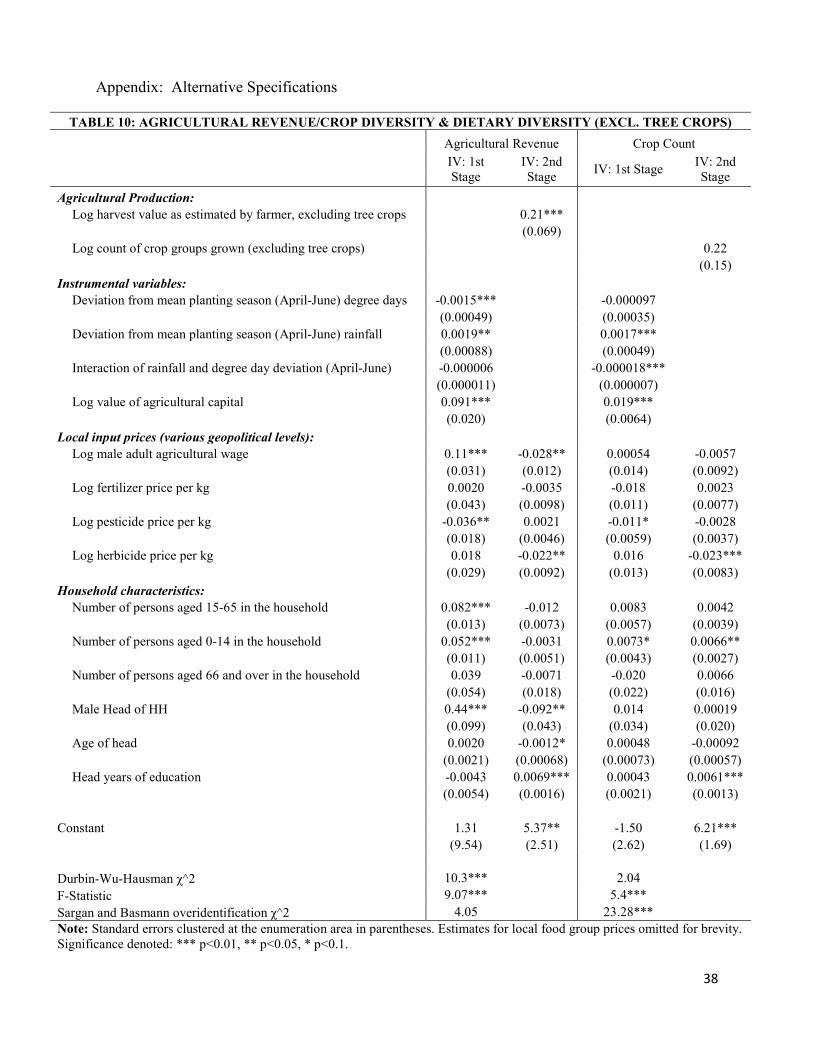
Appendix: Alternative Specifications

TABLE 10: AGRICULTURAL REVENUE/CROP DIVERSITY & DIETARY DIVERSITY (EXCL. TREE CROPS)

Agricultural Revenue Crop Count IV: 1st Stage

IV: 2nd Stage IV: 1st Stage IV: 2nd

Stage Agricultural Production:

Log harvest value as estimated by farmer, excluding tree crops 0.21***

(0.069)

Log count of crop groups grown (excluding tree crops)

0.22

(0.15)


Deviation from mean planting season (April-June) degree days -0.0015***

-0.000097

(0.00049)

(0.00035)

Deviation from mean planting season (April-June) rainfall 0.0019**

0.0017***

(0.00088)

(0.00049)

Interaction of rainfall and degree day deviation (April-June) -0.000006

-0.000018***

(0.000011)

(0.000007)


0.019***

(0.020)


Log male adult agricultural wage 0.11*** -0.028** 0.00054 -0.0057

(0.031) (0.012) (0.014) (0.0092)

Log fertilizer price per kg 0.0020 -0.0035 -0.018 0.0023

(0.043) (0.0098) (0.011) (0.0077)

Log pesticide price per kg -0.036** 0.0021 -0.011* -0.0028

(0.018) (0.0046) (0.0059) (0.0037)

Log herbicide price per kg 0.018 -0.022** 0.016 -0.023***

(0.029) (0.0092) (0.013) (0.0083)


Number of persons aged 15-65 in the household 0.082*** -0.012 0.0083 0.0042

(0.013) (0.0073) (0.0057) (0.0039)

Number of persons aged 0-14 in the household 0.052*** -0.0031 0.0073* 0.0066**

(0.011) (0.0051) (0.0043) (0.0027)

Number of persons aged 66 and over in the household 0.039 -0.0071 -0.020 0.0066

(0.054) (0.018) (0.022) (0.016)

Male Head of HH 0.44*** -0.092** 0.014 0.00019

(0.099) (0.043) (0.034) (0.020)

Age of head 0.0020 -0.0012* 0.00048 -0.00092

(0.0021) (0.00068) (0.00073) (0.00057)

Head years of education -0.0043 0.0069*** 0.00043 0.0061***

(0.0054) (0.0016) (0.0021) (0.0013)

Constant 1.31 5.37** -1.50 6.21***

(9.54) (2.51) (2.62) (1.69)

Durbin-Wu-Hausman χ^2 10.3***

2.04 F-Statistic 9.07***

5.4***

Sargan and Basmann overidentification χ^2 4.05 23.28*** Note: Standard errors clustered at the enumeration area in parentheses. Estimates for local food group prices omitted for brevity. Significance denoted: *** p<0.01, ** p<0.05, * p<0.1.

38

TABLE 11: AGRICULTURAL REVENUE AND DIETARY DIVERSITY

WITH VALUE OF DURABLE ASSETS

2nd Stage

IV w/ Durables

Agricultural Production:

Log value of harvest 0.17***

(0.058)

Local input prices (various geopolitical levels):

Log of local male adult agricultural wage -0.026**

(0.011)

Log of local fertilizer price per kg -0.0042

(0.0087)

Log of local pesticide price per kg 0.00076

(0.0037)

Log of local herbicide price per kg -0.017*

(0.0090)


Number of persons aged 15-65 in the household -0.011*

(0.0059)

Number of persons aged 0-14 in the household -0.0015

(0.0041)

Number of persons aged 66 and over in the household 0.00041

(0.018)

Male Head of HH -0.075**

(0.035)

Age of head -0.0013*

(0.00066)

Head years of education 0.0053***

(0.0016)

Log value of household durables in PH 0.0068

(0.0062)

Constant 4.50**

(2.08)

Durbin-Wu-Hausman χ^2 9.02*** F-Statistic 12.64*** Sargan and Basmann overidentification χ^2 4.27 Note: Standard errors clustered at the enumeration area in parentheses. Estimates for local food group prices omitted for brevity. Significance denoted: *** p<0.01, ** p<0.05, * p<0.1.

39

agricultural production, dietary diversity, and climate

Documents