agricultural growth program (agp) of ethiopia baseline
TRANSCRIPT
Agricultural Growth Program (AGP) of Ethiopia –
Baseline Report 2011
Guush Berhane, Mekdim Dereje, John Hoddinott, Bethelehem Koru, Fantu Nisrane,
Fanaye Tadesse, Alemayehu Seyoum Taffesse, Ibrahim Worku, and Yisehac Yohannes
International Food Policy Research Institute
December 13, 2012
* Address for correspondence: Alemayehu Seyoum Taffesse, email: [email protected]
ii
TABLE OF CONTENTS
ACKNOWLEDGMENTS .................................................................................................................................... XII
EXECUTIVE SUMMARY ..................................................................................................................................... 1
CHAPTER 2 ............................................................................................................................................................. 1 CHAPTER 3 ............................................................................................................................................................. 1 CHAPTER 4 ............................................................................................................................................................. 2 CHAPTER 5 ............................................................................................................................................................. 4 CHAPTER 6 ............................................................................................................................................................. 7 CHAPTER 7 ............................................................................................................................................................. 9 CHAPTER 8 ............................................................................................................................................................. 9 LOG-FRAME INDICATORS ......................................................................................................................................... 10 LOG-FRAME INDICATORS – BASELINE LEVELS ............................................................................................................... 17 ANNEX TO THE EXECUTIVE SUMMARY ........................................................................................................................ 30
CHAPTER 1: THE AGP BASELINE SURVEY — METHODOLOGY AND IMPLEMENTATION ................................... 53
1.1. BACKGROUND........................................................................................................................................ 53 1.2. OBJECTIVES OF THE IMPACT EVALUATION OF THE AGP .................................................................................. 55 1.3. METHODOLOGY — IMPACT EVALUATION .................................................................................................... 55 1.4. METHODOLOGY — SAMPLE DESIGN .......................................................................................................... 60 1.5. METHODOLOGY — HOUSEHOLD AND COMMUNITY QUESTIONNAIRES .............................................................. 64 1.6. DATA COLLECTION .................................................................................................................................. 66
CHAPTER 2: CHARACTERISTICS OF HOUSEHOLDS ........................................................................................... 68
2.1. DEMOGRAPHIC CHARACTERISTICS .............................................................................................................. 68 2.2. EDUCATIONAL CHARACTERISTICS OF HOUSEHOLDS ........................................................................................ 76 2.3. OCCUPATION OF HOUSEHOLD HEADS AND MEMBERS ................................................................................... 78 2.4. OWNERSHIP OF ASSETS ........................................................................................................................... 80 2.5. SUMMARY ............................................................................................................................................ 83
CHAPTER 3: CHARACTERISTICS OF CROP PRODUCTION AND DECISION MAKING ........................................... 85
3.1. CHARACTERISTICS OF CROP PRODUCTION .................................................................................................... 85 3.2. DECISION MAKING IN AGRICULTURE .......................................................................................................... 88 3.3. SUMMARY ............................................................................................................................................ 91
CHAPTER 4: PRODUCTIVITY IN AGRICULTURE ................................................................................................ 92
4.1. PRODUCTIVITY IN THE CROP SUB-SECTOR .................................................................................................... 92 4.2. PRODUCTIVITY IN THE LIVESTOCK SUB-SECTOR ........................................................................................... 101 4.3. LIVESTOCK OWNERSHIP ......................................................................................................................... 102 4.4. SUMMARY .......................................................................................................................................... 105
CHAPTER 5: INPUT USE IN CROP PRODUCTION ............................................................................................ 107
5.1. LAND ................................................................................................................................................. 107 5.2. LABOUR USE ........................................................................................................................................ 115 5.3. MODERN INPUTS USE ........................................................................................................................... 117 5.4. FACTORS CONTRIBUTING TO LOW LEVELS OF USE OF MODERN INPUTS AND PRODUCTION METHODS ...................... 125
CHAPTER 6: UTILIZATION AND MARKETING OF CROPS, LIVESTOCK, AND LIVESTOCK PRODUCTS ................. 131
6.1. CROP UTILIZATION AND MARKETING ........................................................................................................ 131 6.2. LIVESTOCK MARKETING ......................................................................................................................... 145 6.3. DAIRY MARKETING ............................................................................................................................... 152 6.4. SUMMARY .......................................................................................................................................... 155
CHAPTER 7: WAGE EMPLOYMENT AND NONFARM BUSINESSES .................................................................. 157
7.1. PARTICIPATION IN WAGE EMPLOYMENT AND NONFARM BUSINESS ................................................................ 157 7.2. TYPES OF WAGE EMPLOYMENT AND NONFARM BUSINESS ACTIVITIES ............................................................ 159

iii
7.3. SUMMARY .......................................................................................................................................... 172
CHAPTER 8: FOOD SECURITY, NUTRITION, AND HEALTH OUTCOMES ........................................................... 173
8.1. HOUSEHOLD FOOD SECURITY .................................................................................................................. 173 8.2. HOUSEHOLD DIET, AND CHILD NUTRITION AND FEEDING PRACTICES .............................................................. 177 8.3. CHILD AND ADULT HEALTH ..................................................................................................................... 183 8.4. SUMMARY .......................................................................................................................................... 187
REFERENCES ................................................................................................................................................. 189
ANNEXES 190
LIST OF TABLES
Table ES.0.1. Indicators to be fully addressed in the evaluation work ..................................................... 12
Table ES.0.2. Indicators to be partially covered in the evaluation work ................................................. 14
Table ES.0.3. Indicators that will not be covered in the evaluation work due to low level of answerability .................................................................................................................................................................... 16
PDO 1 (National) – Agricultural yield1, by AGP Status .................................................................................... 19
PDO 1 (Regional) – Agricultural yield1, by region ............................................................................................. 20
PDO 2 (National) – Total value of marketed agricultural products per household at current and constant prices (in ETB), by AGP Status ................................................................................................................ 21
PDO 2 (Regional) – Total value of marketed agricultural products per household at current and constant prices (in ETB), by AGP Status and by Region .................................................................................. 22
IO 1.1 (National) – Percentage of farmers satisfied with quality of extension services provided, by AGP Status .................................................................................................................................................................... 23
IO 1.1 (Regional) – Percentage of farmers satisfied with quality of extension services provided by region ............................................................................................................................................................................. 24
IO 2.3 (National) – Area under irrigation (level and per cent of cultivated land) by AGP Status .. 25
IO 2.3 (Regional) – Area under irrigation (level per cent of cultivated land), by region and AGP status .................................................................................................................................................................................... 26
IO 2.4 (National) – Percentage of households practicing soil conservation and water harvesting, by AGP status .................................................................................................................................................................... 27
IO 2.4 (Regional) – Percentage of households practicing soil conservation and water harvesting, by region. ............................................................................................................................................................................ 28
IO.2.5.Community level information on travel time to the nearest market centre (with a population of 50,000 or more) in hours ................................................................................................................ 29
Table ES.1 – Percentage of Kebeles with farmer organizations and the services they provide, by AGP status (related to IO 1.2) .................................................................................................................................... 30
Table ES.2 – Percentage of households using chemical fertilizer, improved seed and irrigation by AGP Status (related to IO 1.3) .................................................................................................................................... 30
Table ES.3 – Percentage of households using chemical fertilizer, improved seed and irrigation (related to IO 1.3) ............................................................................................................................................................ 31
Table ES.4 – Transport Cost (Birr per quintal) to the nearest market in …............................................ 32
Table ES.5 – Transport Cost per Quintal to the nearest market in … ........................................................ 33

iv
Table ES.6Percentage of EAs with farmer organizations and the services they provide, by AGP status and region ............................................................................................................................................................. 34
Table ES.7 Distance to the nearest town and type of first important road, by region and AGP status. ................................................................................................................................................................................... 35
Table ES.8 Accessibility of the first most important road, by region and AGP status. ....................... 35
ES.9. – Cell phone, and radio access and quality of services, by region and AGPstatus. .................... 36
Table ES.10. Access to markets and services, by region and AGP status ................................................. 36
Table ES.11. Yield in quintals for major cereals, pulses and oil seeds by AGP status and egion .... 37
Table ES.12. Milk yield in litre per cow per day by AGP status and region ............................................ 38
Table ES.13. Percentage of households visited by extension agents in the last 12 months............. 39
Table ES.14. Extension service provided for major cereals, pulses and oil seeds on preparation of land ....................................................................................................................................................................................... 39
Table ES.15. Extension service provided for major cereals, pulses and oil seeds on methods of planting ............................................................................................................................................................................... 40
Table ES.16. Extension service provided for major cereals, pulses and oil seeds on methods of fertilizer use ...................................................................................................................................................................... 40
Table ES.17. Satisfaction of households with the last visit by extension agents (crop, livestock and natural management experts) -percentage of households ................................................................... 41
Table ES.18. Satisfaction of households with the last visit by crop expert -percentage of households ......................................................................................................................................................................... 42
Table ES.19 - Satisfaction of households with the last visit by livestock expert (including veterinary services) -percentage of households ................................................................................................ 43
Table ES.20 – Satisfaction of households with the last visit by natural resource management expert -percentage of households ............................................................................................................................ 44
Table ES.21 – Satisfaction of households with the last visit to FTCs -percentage of households .. 45
Table ES.22. Yield in quintals for root crops, chat, enset, and coffee by AGP status and region .... 46
Table ES.23. Extension service provided for root crops, chat, enset, and coffee on preparation of land by AGP status and region ................................................................................................................................... 47
Table ES.24. Extension service provided for root crops, chat, enset, and coffee on seed planting methods by AGP status and region .......................................................................................................................... 47
Table ES.25. Extension service provided for root crops, chat, enset, and coffee on methods of fertilizer use by AGP status and region .................................................................................................................. 48
Table ES.26. Percentage of communities (EAs) who reported to have had community level public work projects undertaken since 2009 and completed by AGP woreda ................................................... 48
Table ES.27. Percentage of communities (EAs) who reported to have had community level public work projects undertaken since 2009 and completed by region and AGP woreda ............................ 49
Table ES.28. Average and proportion of revenue collected from the sale of livestock products by region and AGP status ................................................................................................................................................... 50
Table ES.29. Average and proportion of revenue collected from the sale of crops, by region and AGP status .......................................................................................................................................................................... 51
Table ES.30. Average and proportion of revenue collected from the sale of livestock products by region and AGP status ................................................................................................................................................... 52

v
Table 1.1. Sample size and distribution ................................................................................................................. 62
Table 1.2. Household composition of EA sample ............................................................................................... 63
Table 1.3. AGP program indictors and questionnaire sections .................................................................... 65
Table 2.1. Descriptive statistics on household head’s age by household categories and AGP status ................................................................................................................................................................................................ 69
Table 2.2. Proportion of household head marital status by household categories and AGP status ................................................................................................................................................................................................ 70
Table 2.3. Average household size by household categories and AGP status ........................................ 72
Table 2.4 Percentage of households with average age of members for different age groups by AGP status and household categories ..................................................................................................................... 74
Table 2.5. Percentage of households with an average number of children under 5 years old (in months) of age groups by household categories and AGP status ............................................................... 75
Table 2.6. Percentage of household heads with different education level by household categories and AGP status ................................................................................................................................................................. 76
Table 2.7. Percentage of household members on education level by age and gender ....................... 78
Table 2.8. Percentage of household head’s occupation by household categories and AGP status 79
Table 2.9. Percentage of household head’s occupation of non-head members by household categories and AGP status ........................................................................................................................................... 80
Table 2.10. Percentage of household head’s that used different materials to construct their dwelling by household categories and AGP status ............................................................................................ 81
Table 2.11. Percentage of household head’s asset ownership structure by household categories and AGP status ................................................................................................................................................................. 82
Table 2.12. Average animal ownership by animal type, AGP status and household categories .... 83
Table 3.1. Number of plots cultivated in Meher 2010/11 by household categories and AGP status ................................................................................................................................................................................................ 86
Table 3.2. The distribution of plots by crop type, household categories, and AGP status (percent) ................................................................................................................................................................................................ 87
Table 3.3. Proportion of households growing different crops by household categories and AGP status .................................................................................................................................................................................... 88
Table 3.4. Household members that make decision on what crop to plant by AGP status .............. 89
Table 3.5. Household members that make decision on marketing of crop by household categories and AGP status ................................................................................................................................................................. 90
Table 3.6. Proportion of household members that make decisions on livestock and livestock products by household head categories ................................................................................................................ 91
Table 4.2. Average plot size (ha), by crop type ................................................................................................... 96
Table 4.3. Average crop yield (quintal/ha)1, by household head characteristics ................................ 97
Table 4.4. Average crop yield1, by AGP status and household head characteristics ........................... 99
Table 4.5. Output per adult equivalent labour-day1, by AGP status and household head characteristics ............................................................................................................................................................... 101
Table 4.6. Livestock ownership, by AGP status and household characteristics ................................. 102
Table 4.7. Grazing land as a share of landholdings, by household .......................................................... 103

vi
categories and AGP status ........................................................................................................................................ 103
Table 4.8. Milk yield in litre per cow per day, by AGP status ..................................................................... 104
and household heads’ characteristics .................................................................................................................. 104
Table 5.1. Average number of plots operated, by household categories, AGP status, and region (100% = all households in that category) .......................................................................................................... 108
Table 5.2. Average household plot area and characteristics of plots, by household categories and AGP status ....................................................................................................................................................................... 109
Table 5.3. Average household cultivated area (ha), by household categories, AGP status, and region ................................................................................................................................................................................ 110
Table 5.4. Average area cultivated by crop, by household categories, AGP status and crop classification ................................................................................................................................................................... 113
Table 5.6. Average family labour used (in adult equivalent labour days)1 per hectare of crop, by household categories, AGP status, and crop ..................................................................................................... 117
Table 5.7. Proportion of chemical fertilizer users and average application rate of fertilizer on a plot of land for all farmers and users only (in kg), by household categories and AGP status ...... 118
Table 5.8. Total chemical fertilizer use per crop by household categories and AGP status (kg/ha) ............................................................................................................................................................................................. 119
Table 5.9. Total chemical fertilizer use intensity, by household categories, AGP status, and crop classification for fertilizer users (kg/ha) ........................................................................................................... 121
Table 5.10. Trends in fertilizer application, by household categories, AGP status, and region (% of all households using chemical fertilizer) ...................................................................................................... 122
Table 5.11. Improved seed use, irrigation, and soil conservation, by household categories and AGP status (100%=all farmers) ............................................................................................................................. 123
Table 5.12. Main help from extension agents’ visit, by household categories and AGP status .... 125
Table 5.13. Constraints to fertilizer adoption — proportion of households reporting as most important constraint to adoption (%), by household categories and AGP status............................. 126
Table 5.14. Availability of modern inputs — proportion of households reporting availability in time (%), by household categories and AGP status (100% = all households) .................................... 127
Table 5.15. Percentage of households that purchased Dap with credit and reasons for not using credit, by AGP status and household categories ............................................................................................. 128
Table 5.16. Main reason for not being visited by extension agents, by household categories and AGP status (%) .............................................................................................................................................................. 130
Table 6.1. Crop use (%), by AGP status, household categories, and crop type (100%=total crop production) ..................................................................................................................................................................... 133
Table 6.2. Average revenue per household from crop sales ...................................................................... 134
Table 6.3.a. Average household revenue, , by household categories, and crop types [for households who sold these crops] ........................................................................................................................ 135
Table 6.3.b. Average household revenue, by AGP status, household categories, and crop types [for households who sold these crops] ............................................................................................................... 136
Table 6.4. Average household revenue from crop sales and percentage share by crop class, by AGP status, household categories, and crop types [for all households] ................................................ 139
Table 6.5. Percentage of total crop sales' revenue used for transportation, by AGP status, household categories, and crop type ................................................................................................................... 141

vii
Table 6.6. Major buyers and major reasons for sellers’ choice of buyers, by AGP status, household categories, and crop type [for households who sold these crops] .......................................................... 143
Table 6.7. Proportion of households that used mobile phones in crop sale transaction and that agreed prices over the mobile phone, if used, by AGP status, household categories, and crop type [for households who sold these crops] ............................................................................................................... 144
Table 6.8. Average and proportion of revenue collected from sale of livestock products, by household category, AGP status, and livestock type ..................................................................................... 146
Table 6.9. Proportion of revenue paid for transportation, by household and livestock category and AGP status .............................................................................................................................................................. 147
Table 6.10. Proportion of households that used mobile phone for livestock sales transaction and those that agreed on a price on the phone, if used, by household categories, AGP status, and livestock categories ..................................................................................................................................................... 150
Table 6.11. Average revenue and share of different categories in total revenue of livestock products ........................................................................................................................................................................... 152
Table 6.12. Average travel time to the market place and proportion of revenue paid for transportation, by household category and AGP status ............................................................................... 153
Table 7.1. Percentage of households with wage employment or nonfarm .......................................... 158
businesses, by household categories and AGP status ................................................................................... 158
Table7.2. Percentage of households, by type of wage employment, by household categories, and AGP status [for households that earn wages] .................................................................................................. 161
Table7.3. Percentage of households, by nonfarm business activities, household categories, and AGP status [for households that have nonfarm business activities] ...................................................... 165
Table7.4. Market for selling products/services of nonfarm businesses, by household categories and AGP status [for households that have nonfarm business activities] .............................................. 166
Table7.5. Percentage of households who received technical assistance or credit for their nonfarm business activities, by household categories and ........................................................................ 167
AGP status [for households that have nonfarm business activities] ...................................................... 167
Table 7.6. Reason for not borrowing to finance nonfarm business (percentage of households that not borrowed), by household categories and AGP status ........................................................................... 171
Table 8.1. Primary source of food, by month and gender of household head (percentage of households) .................................................................................................................................................................... 175
Table 8.2. Primary source of food, by month and age of household head ............................................ 175
(percentage of households) ..................................................................................................................................... 175
Table 8.3. Child feeding practices by age (100%=all children in particular age group) ................ 179
Table 8.4. Child feeding practices by age and AGP woreda (100%=all children in particular age group) ............................................................................................................................................................................... 180
Table 8.5. Measures of malnutrition, by household categories and AGP status ................................ 182
Table 8.6. Percentage of children under the age of five with common diseases, by household categories and AGP status ........................................................................................................................................ 184
Table 8.7. Source of drinking water and water treatment, by household ............................................ 187
categories and AGP status ........................................................................................................................................ 187

viii
LIST OF FIGURES
Figure 1.1. AGP woredas .............................................................................................................................................. 54
Figure 1.2. Measuring impact from outcomes from beneficiary and comparison groups ................ 56
Figure 2.1. Distribution of household size ........................................................................................................... 71
Figure 2.2. Age Structure of household members ............................................................................................. 73
Figure 2.3. Proportion of children under 5 years of age ................................................................................. 75
Figure 4.1 Shares in cultivated area and grain output .................................................................................... 92
Figure 4.2. Average household cereal production in kg, by output quintiles ........................................ 95
Figure 4.3. Average cereal yield, by yield quintiles (kg/ha) .......................................................................... 98
Figure 5.1. Distribution of household’s cultivated area ............................................................................... 111
Figure 6.1. Variation of revenue from crop sales among households that actually sold crops ... 140
Figure 6.2. The three largest buyers and their corresponding shares from total sales (%) ......... 148
Figure 6.3. The three most important reasons for sellers' choice of buyer and their corresponding shares (%) ........................................................................................................................................ 149
Figure 6.4. Distribution of revenue from livestock products (percent) ................................................ 151
Figure 6.5. The three largest buyers of dairy products and their share from total sales ............... 154
Figure 6.6. The three most important reasons for choices of dairy product buyers and their respective share ............................................................................................................................................................ 154
Figure 7.1. Percentage of households with wage employment and nonfarm businesses ............. 157
Figure 7.2. Percentage of households, by type of wage employment and ............................................ 159
AGP status [for households that earn wages] .................................................................................................. 159
Figure 7.3. Percentage of households with wage employment, by ......................................................... 160
type of wage employment and month ................................................................................................................. 160
Figure 7.4. Percentage of households by place of wage employment, by ............................................. 162
AGP status [for households that earn wages] .................................................................................................. 162
Figure 7.5. Percentage of households by nonfarm business activities and AGP status [for households that have nonfarm business activities] ...................................................................................... 163
Figure 7.6. Months in which households had business activity for the most and fewest number of days (percentage of households with nonfarm business activities) ...................................................... 164
Figure 7.7. Source of technical assistance and credit .................................................................................... 168
Figure 7.8. Source of technical assistance and credit (percentage of households ............................ 169
with nonfarm business activities receiving assistance/credit), by AGP status .................................. 169
Figure 7.9. Reasons for not borrowing by AGP status (percentage of households ........................... 170
that did not borrow) ................................................................................................................................................... 170
Figure 8.1. Primary source of food by month (percentage of households) ......................................... 174
Figure 8.2. Primary source of food by AGP status (100%=all households) ......................................... 176

ix
Figure 8.3. Average number of months household was food insecure, by household categories and AGP status .............................................................................................................................................................. 177
Figure 8.4. Household dietary diversity score, by household category and AGP status................. 178
Figure 8.5. Percentage of malnourished children under the age of five, by gender ......................... 182
Figure 8.6. Percentage of children under the age of five with common diseases, by AGP status 184
Figure 8.7.a. Percentage of households with at least one member having a hearing or vision problem, by household categories and AGP status ........................................................................................ 185
Figure 8.7.b. Percentage of households with at least one member having a disability caused by injury or accident, by household categories and AGP status ..................................................................... 186
Annex Figure B.4.3. Average household production, by output quintile and AGP status .............. 199
ANNEXES
Annex A: AGP Details .................................................................................................................................................. 190
Annex Table A.1.1. List of AGP woredas ............................................................................................................. 190
Annex Table A.1.2. Sampled AGP-woredas ....................................................................................................... 191
Annex Table A.1.3. Sampled Non-AGP woredas .............................................................................................. 192
Annex B: Tables ............................................................................................................................................................ 193
Annex Table B.2.1. Descriptives statistics on household head’s age, by region and AGP status . 193
Annex Table B.2.2. Proportion of household head’s marital status, by region and AGP status ... 193
Annex Table B.2.3. Average household size, by region and AGP status ................................................ 194
Annex Table B.2.4. Percentage of households with members of different age groups, by region and AGP status .............................................................................................................................................................. 194
Annex Table B.2.5. Percentage of households with children under 5 years old of different age groups, by household categories and AGP status ........................................................................................... 195
Annex Table B.2.6. Percentage of household heads with different education level, by region and AGP status ....................................................................................................................................................................... 195
Annex Table B.2.7.Percentage of household heads’ occupation of by region and AGP status ..... 196
Annex Table B.2.8.Percentage of household heads that used different materials to construct their dwelling, by region and AGP status ...................................................................................................................... 196
Annex Table B.2. 9. Percentage of household heads’ asset ownership structure, by region and AGP status ....................................................................................................................................................................... 197
Annex Table B.2.10. Average animal ownership by animal type, by region and AGP status........ 197
Annex Table B.2.11. Average animal ownership by animal type, by region and AGP status (average for those who own the respective animals) ................................................................................... 198
Annex Figure B.4.1. Share of crops in total acreage, by AGP status ........................................................ 198
Annex Figure B.4.2. Average household cereals production, by output quintiles and AGP status ............................................................................................................................................................................................. 199
Annex Table B.4.1. Mean Difference (MD) test – Average output (in kg), by household head characteristics, AGP status, and crop classification ....................................................................................... 200
x
Annex Table B.4.2. Average output (kg) by region and AGP status ........................................................ 201
Annex Table B.4.3. Mean Difference test - Average yield by household head characteristics, AGP status and crop classification .................................................................................................................................. 202
Annex Table B.4.4. Average crop yield (kg/ha), by AGP status and region ......................................... 203
Annex Table B.4.4. Family labour use – Output per labour day in adult equivalent units, by region and AGP status .............................................................................................................................................................. 204
Annex Table B.4.5. Livestock ownership, by type, region, and AGP status .......................................... 205
Annex Table B.4.6. Milk yield in liters per cow per day, by AGP status and household heads’ characteristics ............................................................................................................................................................... 206
Annex Table B.5.1. Proportion of chemical fertilizer users (%), by crop and household categories ............................................................................................................................................................................................. 207
Annex Table B.5.2. Proportion of chemical fertilizer users and average application rate of fertilizer for all farmers and users only (in kg), by household categories and AGP status ........... 208
Annex Table B.5.3. Improved seed, irrigation, and soil conservation use by region and AGP status (% of households) ........................................................................................................................................................ 208
Annex Table B.5.4. Improved seed use by AGP status, household head characteristics and crop type (% of households).............................................................................................................................................. 209
Annex Table B.5.5. Improved seed use, by region, AGP status, and crop type (% of households) ............................................................................................................................................................................................. 209
Annex Table B.5.6. Mean difference test – Proportion of households using improved seed, by crop type and household categories .................................................................................................................... 210
Annex Table B.5.7. Percentage of households that purchased improved seed with credit and reasons for not using credit, by AGP status and household categories ................................................. 210
Annex Table B.6.1. Crop use (%), by region, crop, and AGP status (100%=total crop production) ............................................................................................................................................................................................. 212
Annex Table B.6.2. Average revenue (ETB) from crop sale, by region, AGP status, and crop type ............................................................................................................................................................................................. 213
Annex Table B.6.3. Percentage of households who sold their output, by crop type, household categories, and AGP status ....................................................................................................................................... 214
Annex Table B.6.4. Percentage of households who sold their output, by crop type, region, and AGP status ....................................................................................................................................................................... 215
Annex Table B.6.5. Percentage of transportation cost from total revenue, by region, AGP status and crop type ................................................................................................................................................................. 215
Annex Table B.6.6. Major buyers and major reasons for the choice of buyers, by region and crop type. ................................................................................................................................................................................... 216
Annex B.6.7. Proportion of households that used mobile phone in crop transaction and those that agreed price over mobile phone, if used, by region and crop type ................................................ 217
Annex Table B.6.8. Average and proportion of revenue collected from the sale of livestock types, by region .......................................................................................................................................................................... 217
Annex Table B.6.9. Proportion of revenue paid for transportation, by region. .................................. 217
Annex Table B.6.10. Proportion of households that used mobile phone and that agreed price using mobile, if used, by region .............................................................................................................................. 218

xi
Annex Table B.6.11. Average and proportion of revenue collected from the sale of livestock products, by region ..................................................................................................................................................... 218
Annex Table B.6.12. Average travel time to the market place and proportion of revenue paid for transportation, by household category and AGP status. .............................................................................. 218
Annex C: Description of Survey Areas based on Community Questionnaire Data ........................... 219
Annex Table C.1.1. Distance to the nearest town and type of first important road, by region and AGP status. ...................................................................................................................................................................... 221
Annex Table C.1.2. Accessibility of the first most important road, by region and AGP status. .... 222
Annex Table C.1.3. Tap water access and sources of drinking water, by region and AGP status. ............................................................................................................................................................................................. 225
Annex Table C.1.4. Electricity, cell phone, and radio - access and quality of services, by region and AGP status. ............................................................................................................................................................. 226
Annex Table C.1.5. Access to markets and services, by region and AGP status ................................. 230
Annex Table C.1.6. Number of schools in PAs and distances travelled where unavailable, by region and AGP status ................................................................................................................................................ 232
Annex Table C.1.7. Access to health facilities in PAs and distances travelled where unavailable, by region and AGP status .......................................................................................................................................... 234
Annex Table C.1.8. Availability, sufficiency, and criteria for allocation of fertilizer and improved seeds, by region and AGP status ............................................................................................................................ 239
Annex Table C.1.9. Access to and quality of extension services, by region and AGP status .......... 243
Annex Table C.1.10. Distribution of saving and credit cooperatives (SCCs) and services they provided, by region and AGP status. .................................................................................................................... 245
Annex Table C.1.11. Distribution of savings and loan cooperatives (SLCs) and services they provided, by region and AGP status. .................................................................................................................... 246
Annex Table C.1.12. Distribution of producers associations (PAs) and services they provided, by region and AGP status. ............................................................................................................................................... 247
Annex Table C.1.13. Distribution of banks and small microfinance institutions (MFIs) and services provided by MFIs, by region and AGP status .................................................................................. 248

xii
Acknowledgments
We thank USAID for funding and the World Bank for facilitating the work undertaken to
produce this report. We also would like to acknowledge the support of the Agricultural
Growth Program Technical Committee (AGP-TC) throughout the conduct of the AGP
baseline survey and the preparation of the report. The Ethiopian Central Statistical
Agency (CSA) ably implemented the household and community surveys on which this
report is based. We especially thank Weizro Samia Zekaria and Ato Biratu Yigezu,
respectively, Director-General and Deputy Director-General of the CSA, for their support.
Most importantly, we thank the thousands of Ethiopians who answered our many
questions about themselves and their lives. The authors of this report are solely
responsible for its contents.

1
Executive Summary
Chapter 2
This chapter provides an overview of the demographic structure of households
which are covered by the Agricultural Growth Program (AGP) baseline survey. The
chapter reports descriptive analysis of demographic variables like age and size
distribution of the households, marital status, education, and occupation of the
household heads and household members. In the discussion, emphasis is also
given to differences between genders, age groups and AGP status classification.
The average age for the household head is about 43 years while female headed
households tend to be older. Regarding marital status of heads, the majority of
household heads are married. There are more female headed households who are
separated or divorced compared to male heads. However, there is no notable
difference across households in AGP and non-AGP woredas. The surveyed
households have on average five members with relatively smaller size for
households with younger heads. However, there is little difference in household
size distribution across AGP classification. Detailed statistics are also computed
across age cohorts.
Regarding the educational status, about 54 percent of the household heads
surveyed are illiterate. When looked across gender, the large majority of the
female household members are illiterate. From those who attended formal
education, the majority are households with young heads while a higher
proportion of mature heads have some sort of informal education. Notable
differences also exist among the different age groups. The occupational structure
of households shows that about 89 percent of the household heads surveyed are
farmers or family farm workers and the proportion reaches even about 97 for male
headed households. Female headed households tend to diversify their occupation
to non-agricultural activities.
Chapter 3
The chapter summarises crop production and decision making of households in
the production and sale of crop and livestock products. The surveyed households
cultivated for the Meher season a total number of 46.9 million plots. A significant
percentage of variation was observed in the proportion of plots allocated for each

2
crop category. Cereals took the largest proportion of plots followed by pulses and
coffee. This result holds true for AGP and non-AGP woredas, except in AGP
woredas enset is more important than coffee. Decision making on crop production
and marketing was mostly made by the head or head and spouse. Likewise,
decision on marketing of crop produced is mostly done by the head, followed by
the spouse (though the percentage is much lower). However, a noticeable result
was found when comparing decision making on livestock and livestock products
by gender dimension. Chicken production is mainly controlled by female heads and
spouses. Moreover, decisions regarding the production of milk and milk products
are made by the female heads.
Chapter 4
This chapter focuses on aspects of crop and livestock productivity of households in
the study area. Accordingly, the summarized findings on output levels, yields, and
labour productivity estimates for both crop production and livestock production
are provided. Due emphasis is attached to major crops yields. In order to capture
the output and yield estimates, crops are categorized into fifteen groups — teff,
barley, wheat, maize, sorghum, other cereals, (which at some points are discussed
in group as cereals), pulses, oilseeds, vegetables, fruits, root crops, coffee, chat,
enset, others.
In terms of area cultivated, the first striking feature is the predominance of cereals
which accounted for 66 percent of total acreage. Among cereals, teff recorded the
largest share of cultivated area (16.1 percent), followed by maize (15.2 percent)
and wheat (11.5 percent). Regarding the acreage shares across AGP status
groupings, on average, AGP woredas had larger acreage shares going to teff,
sorghum, and oil seeds. In contrast, non-AGP woredas recorded greater shares for
barley, pulses, and fruits. Although maize and wheat respectively took second and
third place in terms of acreage, they ranked first and second in output with a share
of 30 percent and 17 percent respectively. Teff took the third spot in output with a
share of 13 percent.
Estimates of output at the household level reveal that on average these outputs
were not very high during the Meher season covered. For the study area as a
whole, they range from 1.3 quintals for coffee through to 5.8 quintals for maize.
The median, on the other hand, is 2 quintals, implying that half of these households

3
produced less than 2 quintals. The comparison among AGP groups show that,
among the crops considered, average household output was higher in AGP
woredas relative to non-AGP woredas for teff, wheat, maize, sorghum, pulses, oil
seeds, and chat while average output was greater in non-AGP woredas for the
other crops. Moreover, the only statistically significant differences between
households in AGP and non-AGP woredas were observed for sorghum, pulses, and
oilseeds. To complement on the perspective provided by average output levels,
average plot sizes are also computed. The findings indicate that on average a
household operates plots measuring a third of a hectare. Although the land sizes
allocated to sorghum and oilseeds are the two highest, there was no significant
difference on average plot size allotted to annual crops. When plot sizes are viewed
across gender of household heads, the findings confirm that male headed and
mature headed households had slightly bigger plots compared to those of their
respective counterparts.
Subsequently, average yields for each crop are considered. Among cereals, maize
turned out to have the highest yields (17.2 quintals per hectare), while teff had the
lowest (9.4 quintals per hectare). This ranking held across household groups and
locations. A striking difference has been observed across mean and median
estimates, however. For instance, the mean teff yield of 9.4 quintals per hectare is
matched with a median of 6.7 quintals per hectare. In other words, half of the teff
producers could only achieve teff yields of less than 6.7 quintals per hectare.
Statistically significant differences in mean yields were registered across
household types. Female headed households achieved lower yields in teff, barley,
maize, and root crop production. These differences amounted to 1-2 quintals per
hectare. However, there is no significant difference recorded between AGP and
non-AGP woredas.
Labour productivity is generally characterized in terms of a ratio of the amount of
output produced to the associated amount of labour used. To do so, output per unit
of labour (in adult equivalent labour (or work) day) is estimated. For all farm
households, mean levels of labour productivity measured range from 9.7 kg for
sorghum to 14 kg for barley. It is striking that differences of comparable
magnitude were not recorded among these output levels across household types.
For example, the largest labour productivity shortfall in female headed households
was 1kg in oilseeds production. Similarly, the gap between labour productivity of

4
households in AGP and non-AGP woredas was highest in oilseeds, amounting to 2.8
kg.
Livestock productivity indices are intrinsically more complex with corresponding
data challenges. But some indicative measures are computed. On average, cattle-
owning farm households in the study area owned 3.6 heads of cattle. Male headed
households, mature headed households, and households in AGP woredas owned
more cattle than their counterparts. Availability of grazing land is another major
determinant of not only the number of animals owned but also the corresponding
productivity. Farm households in the study area identified only 6 percent of their
landholdings as grazing area. On average, female headed households allocated a bit
more of their holdings (7.2 percent) to grazing than male headed households (5.8
percent). The average milk yield was about a litre per cow per day and displays
very little variation across household groups or locations. Nevertheless, there is
considerable heterogeneity (relative to the average) in cow milk yields within each
group.
Chapter 5
Chapter 5 provides an overview on the intensity and magnitude of inputs used for crop
production. The major inputs used during the season considered are land, labour, and
modern inputs (fertilizer, improved seeds, soil conservation methods and extension
services).
Land: A total of 45.2 million plots of land were covered by annual and perennial
crops in the study area. On average, during the survey year, a household operated
1.14 ha of land divided into 4.7 plots with the average size of a single plot being
0.25 ha. About half of the households cultivated less than 0.94 ha of land. Male
headed households hold roughly 1.25 ha of land while female heads are found to
possess only 0.89 ha. When we look at the difference across age, larger proportion
of households with young heads operated relatively fewer plots than mature
heads. The calculated statistics also reveal that AGP Woredas tend to have slightly
larger cultivated areas than non AGP woredas.

5
Most of the plots are located at about 19 minutes walking distance from farmers’
residences. Plots cultivated by households headed by male and young heads are
farther away from their homes relative to those operated by female and mature
headed households.
Households were asked to classify their plot as in response to the question slightly
more than half of the cultivated plots were reported to be fertile while were
deemed moderately fertile, only remaining 11 percent were identified as infertile.
Labour: Labour use is measured as the number of adult equivalent work days per
hectare of land by family members. Among cereals, median labour days were
highest maize and teff and least required for cultivating barley and wheat required.
The data show that male headed households used more labour for all crops except
vegetables.
Fertilizer: Although the percentage of households who use fertilizer has increased
over time, the baseline survey indicates that fertilizer application is still low. About
58 percent of households in the study area used chemical fertilizers. Even among
farmers who are using fertilizer, a large proportion of them only apply small
quantities. On average, farm households in the study area applied 27 kg of
chemical fertilizer made up of DAP and urea separately or together. On average,
male-headed and mature–headed households applied more chemical fertilizers
compared to female-headed and young-headed households, respectively. The gap
narrows down considerably when we compare actual users. Relative to
households headed by the young, those with mature heads used 10 percent more
fertilizer. AGP Woreda households on average used 16 percent more fertilizer than
those in non-AGP Woredas. Nevertheless, a large majority (98 percent) of
households reported that they have applied manure in their fields.
The recent trend in fertilizer application is improving over time in both AGP and
non-AGP Woredas. The adoption is increasing at an average annual rate of 6.2
percent although the growth rate is slower for female headed households.
Improved seeds: Out of all plots, about 90 percent were planted with local seeds;
about 1.3 percent with seeds saved from output produced using previously bought
improved seeds, and 6.3 percent with freshly bought improved seeds. The
remaining 2.1 percent were sown with a combination of the three types. While 76

6
percent of the total improved seed was newly bought, the remaining 24 percent
was saved from the output of previously used improved seeds. Although 23.5
percent of the households used improved seeds, the amount used in the study area
averaged less than a kilogram per hectare. However, the application rate of
improved seeds among users was significantly large at about 17.5 kg per hectare.
The proportion of female-headed households that applied improved seeds is 9
percentage points lower than applied by male headed households. Slightly more
households with mature-heads applied improved seeds. Relative to households in
non AGP Woredas more households in AGP Woredas used improved seeds and
average improved seeds application was slightly larger among households in AGP
Woredas.
Irrigation and soil conservation: Among households in the study area only 4.2
percent irrigated their plots while a significantly large proportion (72 percent)
practiced some soil conservation measures. Relative to female-headed households,
the proportions of households with male heads that used irrigation and soil
conservation measures were larger. A relatively larger proportion of AGP
households of all categories irrigated their land relative to the corresponding
categories of non-AGP households.
Extension services: About 35.5 percent of the households were visited by an
extension agent at least once and a quarter said they were visited more than once.
Comparatively, female headed households were less visited than their male
counter parts. Relative to households with mature heads those with young heads
were also visited more. Information provided on new inputs and production
methods were selected by respondents as by far the two most important services
visited households received – 35 percent and 34 percent of the households
selecting the two as most important, respectively. All household groups in all
locations identified the two as important, though the order in which they did so
was not always the same. Extension agents’ help in obtaining fertilizer was the
third important support.

7
Chapter 6
Sales income. Combining sales revenue from three sources (crops, livestock, and
livestock products), it is found that total sales income for an average household in
the survey area over a 12 month period amounts to 4,968 Birr. The majority of the
sales revenue is made up from crop sales revenue, as this category accounts for
70% of the sales income of the average household (3,469 Birr). The revenue from
the sales of livestock comes second, making up 26% of the sales income (1,344
Birr). Sales revenue from livestock products (meat, hides and skins, milk, cheese,
butter, yoghurt, dung, and eggs) are estimated to be relatively less important as
they make up only 3% of the annual sales revenue of an average household (155
Birr).
Crop utilization. One of the salient features of crop production in countries such as
Ethiopia is that households consume a significant fraction of the output they
harvest. This is also found in this dataset. We, however, note significant differences
between crops. For only two crops more than half of the production is sold, i.e. chat
(81%) and oilseeds (68%). Even for a major cash crop as coffee, the majority of the
production is consumed by the household itself (64%) and only 35% of the coffee
production is put up for sale. We note also large differences between the major
cereals. Of all the cereals, teff is used most as a cash crop. A quarter of total
production is being sold. This compares to 58% of its production being used for
own consumption. Sorghum, maize, and barley show the lowest level of
commercialization with a share of production that is being sold ranging from 10%
to 13%. Farmers in the study area further rely little on markets to obtain seeds, as
illustrated by relatively large percentages of the production being retained for seed
purposes, in the case of cereals varying between 6% (maize) and 19% (barley) of
total household production.
Crop sales. The average revenue from crop sales in the survey area in the year prior
to the survey amounts to 3,469 Birr per household. There are large differences
between households and it is estimated that half of the households earned less
than 597 Birr from crop sales income. Coffee is the most important crop in total
crop sales, accounting for 40% of total crop sales followed by wheat accounting for
11% of the total crop sales. This high contribution of coffee to total crop sales
could be driven by the high price of coffee relative to other crops. However, the
percentage of households who are marketing coffee is only 10 percent and mainly

8
concentrated in SNNP (Southern Nations, Nationalities, and Peoples) and Oromiya
regions. Most of the crops are being sold to village traders and few farmers travel
far distances to sell produce as it is found that transportation costs make up a
relatively small percentage of total earnings from sales. Most importantly, most
farmers chose traders because they are able to pay immediately and not because
they offer higher prices. This might reflect lack of trust in traders as well as a
relative large importance of distress sales. It is also found that relatively few
farmers use mobile phones to find traders and agree on prices, partly reflecting the
still relatively low penetration of mobile phones in rural areas of Ethiopia.
Livestock sales. The revenue from livestock sales for an average household in the
survey made up 1,344 Birr in the year prior to the survey. The revenue from
livestock sales compares to 38% of the revenue from crop sales. Within the sales of
livestock, it is especially the sales of cattle that are important as they account for
77% of the total sales. Second come the sales of goats and sheep accounting for
13% of total livestock sales income. Pack animals and chicken each count for 5% of
total livestock sales income. As for the case of crops, expenses for transportation
are relatively less important compared to sales income. The most important reason
for choosing a buyer is linked to cash payments, followed by the prices offered. No
choice in traders is relatively less important as the reason for the choice of selling
to a particular trader but it still makes up 10% of the stated answers for choosing a
trader. It thus seems that farmers in these surveyed areas might benefit from
improved choices in sales options.
Livestock products. The revenues that were generated from the sales of livestock
products amounted to 155 Birr in the year prior to the survey for an average
household. The most important livestock product was the butter/yoghurt category
accounting for 55% of all livestock products sales income. Egg comes second,
accounting for 30% of the livestock product sales. Meat (6%), hides and skins
(4%), fresh milk or cream (4%), and dung (1%) are relatively much less important.
While sales to village traders are still relatively most important, direct sales to
consumers for these products are much more important than for crop and
livestock sales, reflecting the more perishable nature of the majority of these
products. They are thus probably relatively more important for the local economy.
The most important reason for the choice of a buyer is again cash payments (and
less the level of the price offered).
9
Chapter 7
This chapter describes wage employment and nonfarm business activities of the
household in the four regions. Of all the household members, head of the
household takes the largest percentage in the participation of nonfarm business. In
terms of age categories, the involvement of younger household heads in nonfarm
business and wage employment is higher than the matured ones. Although there is
no considerable difference between male and female headed households in the
percentage of households participating in nonfarm and wage employment, female
headed households involved more in selling traditional food/liquor. It was noted in
the survey results that households with young heads are more engaged in livestock
trade than those with matured heads. The major market for selling
products/service for AGP and non-AGP woredas was found to be the same village
they are living in. Male headed households appear to have a better access to
markets outside their own villages while female heads use their own village as a
market place for their products.
The survey results revealed that relatives and friends account for the largest share
of credit source. However, microcredit institutions were found to be one of the
main sources of credit for households living in AGP woredas in order to finance
nonfarm business. Households in the study area were asked to prioritize their
reason for not receiving credit and a large percentage of the households indicated
that they were not interested to take the loan, followed by lack of an institution to
provide loan in their area.
Chapter 8
Most rural households rely on own production to satisfy their food requirements.
Reliance on own-produced food varies mainly with cropping seasons. The largest
proportions of the households rely on own-produced food during and after
harvest. The smallest proportions of households rely on own-produced food
during the raining and planting months in the main agricultural season, during
which a considerable proportion of food is purchased and obtained from other
sources to cover the food need. Moreover, the data indicate that an average
household was food insecure for 1.2 months during the year. Male headed and
households in AGP woredas performed relatively better.

10
The data also indicate that the food items consumed by household members were
less than half as diverse as required for a healthy diet. Although dietary diversity
varied among the different categories and woredas, the variation was small. Long-
and short-term nutritional status of children under the age of 5 was examined
using anthropometric measures collected in the survey. The results indicate a
prevalence of severe stunting, wasting, and underweight in 27, 6, and 10 percent of
the children. The proportion with moderate stunting, wasting, and underweight
was 46, 12, and 27 percent, respectively. Children in households with female and
mature heads and those in non-AGP woredas performed better in all or most
measures. Diarrhoea, coughing, fever, and breathing problems affected 25, 37, 32,
and 15 percent of the children in the 2 weeks prior to the survey.
Less than half of the households have access to safe drinking water and more than
40 percent use the same water for drinking and other purposes. While there were
differences among household categories in access to safe water the differences
were small. Although about 58 percent of the households do not have access to
safe drinking water, less than 10 percent boil the water they drink. The practice is
more prevalent in male and mature headed households.
Log-frame Indicators
The AGP has a set of outcome indicators that defines its intermediate and ultimate
objectives. These are identified in the program’s log frame. The primary objective of the
AGP baseline survey (as well as the planned follow-on surveys and analyses) is to assess
the impact of AGP interventions on the log frame indicators as rigorously as possible.
Ideally, this assessment will answer whether AGP interventions are directly and
exclusively responsible for the recorded changes in these indicators. Nevertheless, there
is considerable cost involved in achieving this ideal. Moreover, not all indicators are
equally important and, in a lot of cases, it may be sufficient to credibly establish that AGP
interventions contributed to changes in the relevant indicators without ascertaining
causality.
Accordingly, the degree of answerability reported below expresses the possible type of
link that can be credibly established between the AGP interventions and the indicators
identified as well as the nature of the analysis used to do so. These reflect the survey

11
sample size as per the decision of the AGP-TC and the survey data collected. The latter,
in turn, reflect the instruments of data collection used (the questionnaires were shared
with AGP-TC members), the characteristics of sample households actually drawn, and
the circumstances of data collection.
The manner of coverage is summarized by three possibilities identified under the
‘Answerability’ column in the tables below. ‘Answerability’ identifies the type of analysis
possible for the corresponding key indicator. The following are the options:
1. Impact Assessment (IA) — Movements in the indicators are tracked and the impact
originating from AGP interventions/investments will be identified and measured.
2. Track Changes (TC) — Movements in the indicators as well as their correlates will
be tracked without necessarily causally identifying those movements with AGP
interventions/investments. There are two sub-options. It is possible to conduct
systematic analysis of the movements of indicators and correlates (TC-A). Or, it is
possible to have descriptive analysis only (TC-D).
3. Not Feasible (NF) — Movements in the indicator cannot be tracked and/or
analysed with reasonable confidence given the data available.
Similarly, the extent of coverage in the proposed evaluation work categorizes the
indicators into three groups. These are:
1. Indicators to be fully addressed – all defining characteristics of the indicator will
be examined;
2. Indicators to be partially covered – key aspects of the indicator will be studied; and
3. Indicators to be not covered, because they are either infeasible or have low level of
answerability.
Tables ES.0.1-ES.0.3 collect the log-frame indicators by the extent of coverage. They also
report on the manner in which these indicators are tracked. The baseline levels of the
indicators are subsequently reported via summary tables while additional tables are
included in the annex to the Executive Summary.

12
Table ES.0.1. Indicators to be fully addressed in the evaluation work
Development objective PDO indicators Available indicator Answerability Reference
table Remark
Agricultural productivity and market access increased for key crop and livestock products in targeted woredas, with increased participation of women and youth.
1. Percentage increase in agricultural yield of participating households (index for basket crops and livestock products).
yield
IA (teff, wheat, barley, maize sorghum, pulses, and oil seeds), TC-A by household type
PDO 1, ES.11,
Attribution to AGP can only be achieved with detailed information about the nature and implementation of the relevant AGP interventions.
yield TC-A (Others crops and milk)
PDO 1, ES.12, ES.22
Systematic analysis can only be achieved with detailed information about the nature and implementation of the relevant AGP interventions.
2. Percentage increase in total real value of marketed agricultural (including livestock) products per participating household.
marketed output IA possible, TC-A more likely
PDO 2, ES.28, ES.29, ES.30
Attribution to AGP and/or systematic analysis can only be achieved with detailed information about the nature and implementation of the relevant AGP interventions.
Intermediate outcome for each component
Outcome indicators for components
Available indicator Answerability Reference
table Remark
Component 1: Agricultural production and commercialization
Sub-component 1.1: Institutional strengthening and development
Farmers have improved access to and quality of services through support from key public institutions and private organizations (groups).
1. Percentage of farmers satisfied with quality of extension services provided (disaggregated by service providers, type of service/technology, crop, and livestock).
percentage of households who received crop level extension advice and the percentage of households satisfied with the advice received (by key types of advice/information)
IA possible, TC-A more likely (teff, wheat, barley, maize, sorghum, pulses, and oil seeds)
IO 1.1, ES.13, ES.14, ES.15, E.16, ES.17, ES.18, ES.19, ES.20, ES.21
Attribution to AGP and/or systematic analysis can only be achieved with detailed information about the nature and implementation of the relevant AGP interventions.

13
Sub-component 1.2: Scaling up best practices
Sub-projects for improved productivity, value addition, and marketing realized and sustainably managed.
3. Number of farm households with innovative best practices (improved/new techniques and technologies).
Percentage of households that used chemical fertilizers, improved seeds, irrigation, water harvesting, soil conservation, and row planting
IA possible, TC-A more likely (chemical fertilizers, improved seeds, and irrigation)
IO 1.1, ES.3
Attribution to AGP and/or systematic analysis can only be achieved with detailed information about the nature and implementation of the relevant AGP interventions.
Component 2: Rural infrastructure development
Sub-component 2.1: Small-scale agricultural water development and management
Demand driven infrastructure investments for improved agricultural productivity realized and sustainable managed.
1. Number of farmers benefiting from the irrigation investments (disaggregated by type of investments).
Percentage of farmers using irrigation on their plot and the percentage of farm land under irrigation
IA possible, TC-A more likely
IO 2.3
Attribution to AGP and/or systematic analysis can only be achieved with detailed information about the nature and implementation of the relevant AGP interventions.
3. Percentage increase in area under irrigation.
Percentage of farm land under irrigation
TC-A IO 2.3
Notes: ‘Answerability’ identifies the type of analysis possible for the corresponding key indicator. The following are the options: 1. Impact Assessment (IA) — Movements in the indicators are tracked and the impact originating from AGP interventions/investments will be identified and measured. 2. Track Changes (TC) — Movements in the indicators as well as their correlates will be tracked without necessarily causally identifying those movements with AGP
interventions/investments. There are two sub-options. It is possible to conduct systematic analysis of the movements of indicators and correlates (TC-A). Or, it is possible to have descriptive analysis only (TC-D).
3. Not Feasible (NF) — Movements in the indicator cannot be tracked and/or analysed with reasonable confidence given the data available.

14
Table ES.0.2. Indicators to be partially covered in the evaluation work
Intermediate outcome for each component
Outcome indicators for components
Available indicator Answerability Reference
table Remark
Component 1: Agricultural production and commercialization
Sub-component 1.1: Institutional strengthening and development
Farmers have improved access to and quality of services through support from key public institutions and private organizations (groups).
1. Percentage of farmers satisfied with quality of extension services provided (disaggregated by service providers, type of service/technology, crop, and livestock).
Percentage of households who received crop level extension advice and the percentage of households satisfied with the advice received (by key types of advice/information)
TC-A (Other crops, livestock)
ES.23, ES.24, ES.25
Systematic analysis can only be achieved with detailed information about the nature and implementation of the relevant AGP interventions.
2. Share of households that are members of functioning farmer organizations (disaggregated by group type).
Community level availability of functioning farmer organizations and their services
TC-A IO 1.2, ES.1, ES.6
Attribution to AGP and/or systematic analysis can only be achieved with detailed information about the nature and implementation of the relevant AGP interventions.
Sub-component 1.2: Scaling up best practices
Sub-projects for improved productivity, value addition, and marketing realized and sustainably managed.
4. Number of sub-projects fully operational and sustainably managed 2 years after initial investments (disaggregated by type of investments).
Community level information on community level public work projects undertaken since 2009 and completed
TC-D ES.26, ES.27
Requires detailed information on the relevant AGP sub-projects.
Sub-component 1.3: Market and agribusiness development
Key selected value chains strengthened.
5. Percentage real sales value increase of the key selected value chains commodities supported at the end of the value chain.
Marketed output TC-A
Systematic analysis can only be achieved with detailed information about the nature and implementation of the relevant AGP interventions.

15
Component 2: Rural infrastructure development
Sub-component 2.1: Small-scale agricultural water development and management.
Demand driven infrastructure investments for improved agricultural productivity realized and sustainably managed.
4. Percentage increase in areas treated under sustainable land management.
Percentage of farmers practicing soil conservation measures
TC-D
Sub-component 2.2: Small-scale market infrastructure development and management
Demand-driven infrastructure investments for improved access to market realized and sustainably managed.
5. Percentage decrease in time for farmers to travel to market centre.
Community level information on travel to the nearest city centre
TC-A IO 2.5
Notes: ‘Answerability’ identifies the type of analysis possible for the corresponding key indicator. The following are the options: 1. Impact Assessment (IA) — Movements in the indicators are tracked and the impact originating from AGP interventions/investments will be identified and measured. 2. Track Changes (TC) — Movements in the indicators as well as their correlates will be tracked without necessarily causally identifying those movements with AGP interventions/investments. There are two sub-options. It is possible to conduct systematic analysis of the movements of indicators and correlates (TC-A). Or, it is possible to have descriptive analysis only (TC-D). 3. Not Feasible (NF) — Movements in the indicator cannot be tracked and/or analysed with reasonable confidence given the data available.
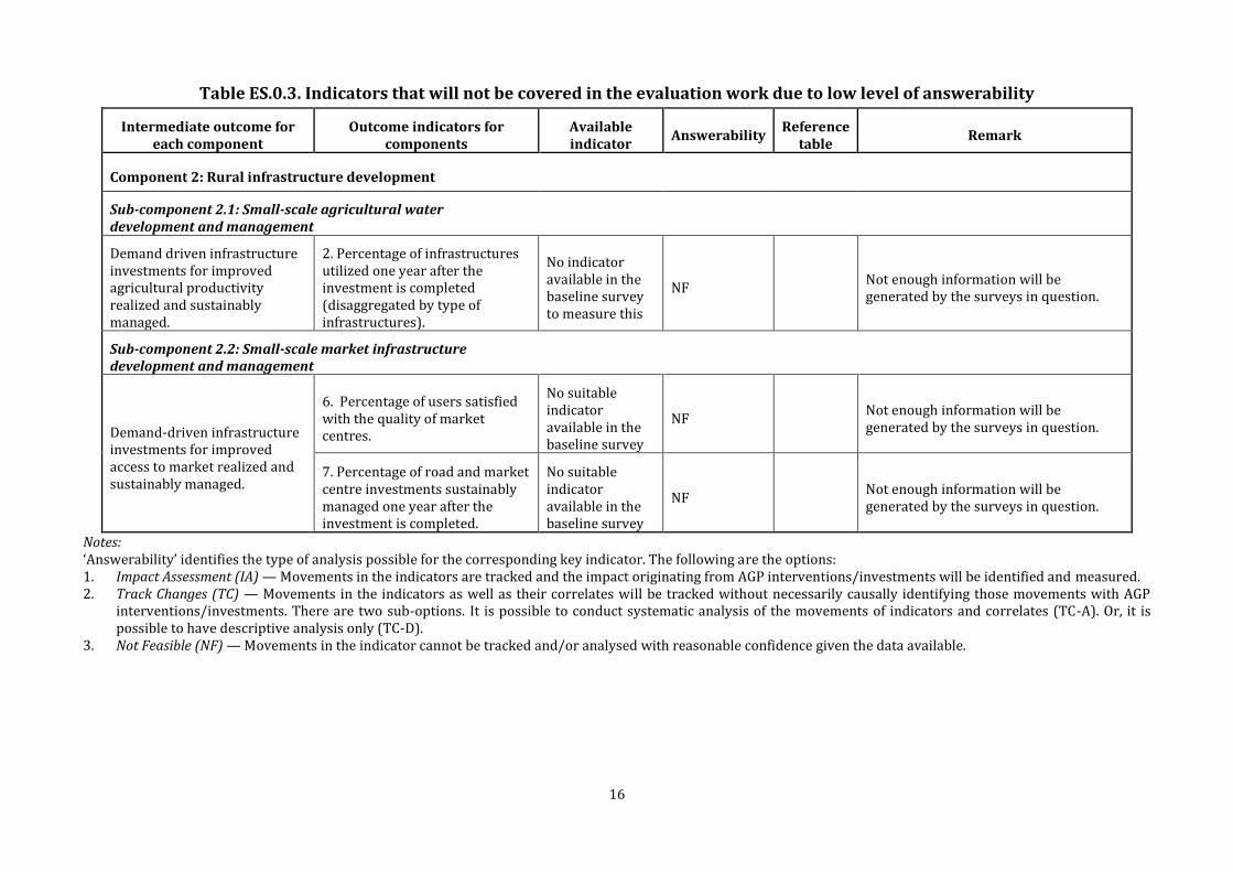
16
Table ES.0.3. Indicators that will not be covered in the evaluation work due to low level of answerability
Intermediate outcome for each component
Outcome indicators for components
Available indicator
Answerability Reference
table Remark
Component 2: Rural infrastructure development
Sub-component 2.1: Small-scale agricultural water development and management
Demand driven infrastructure investments for improved agricultural productivity realized and sustainably managed.
2. Percentage of infrastructures utilized one year after the investment is completed (disaggregated by type of infrastructures).
No indicator available in the baseline survey to measure this
NF Not enough information will be generated by the surveys in question.
Sub-component 2.2: Small-scale market infrastructure development and management
Demand-driven infrastructure investments for improved access to market realized and sustainably managed.
6. Percentage of users satisfied with the quality of market centres.
No suitable indicator available in the baseline survey
NF Not enough information will be generated by the surveys in question.
7. Percentage of road and market centre investments sustainably managed one year after the investment is completed.
No suitable indicator available in the baseline survey
NF Not enough information will be generated by the surveys in question.
Notes: ‘Answerability’ identifies the type of analysis possible for the corresponding key indicator. The following are the options: 1. Impact Assessment (IA) — Movements in the indicators are tracked and the impact originating from AGP interventions/investments will be identified and measured. 2. Track Changes (TC) — Movements in the indicators as well as their correlates will be tracked without necessarily causally identifying those movements with AGP
interventions/investments. There are two sub-options. It is possible to conduct systematic analysis of the movements of indicators and correlates (TC-A). Or, it is possible to have descriptive analysis only (TC-D).
3. Not Feasible (NF) — Movements in the indicator cannot be tracked and/or analysed with reasonable confidence given the data available.

17
Log-frame Indicators – Baseline Levels
The following tables report on the level of AGP log-frame indicators estimated from the AGP
Baseline Survey. The details regarding data collection and estimation of levels are to be
found in the relevant chapters. Two important caveats – one pertaining to disaggregation
and the other to yield estimates – need to be declared at this juncture, however.
Disaggregation
The AGP log-frame (included in the project appraisal document as well as the project
implementation manual) identifies two project development objective (PDO) indicators and
twelve component-level outcome indicators.1 A number of these indicators were to be
disaggregated by region, commodity, and gender and age of household heads. Further, the
impact of AGP on all these has to be rigorously assessed. A survey that can generate
information of sufficient quantity and quality for a rigorous evaluation of AGP’s impact on
each and every one of these indicators will be very large, very expensive as a consequence,
and of doubtful value.
Instead, a sample stratification design reflecting the population shares of the household
types of AGP interest – namely, female and youth-headed households – was implemented.2
As a consequence, it become possible to report all household-level data below as
disaggregated by gender and age of household heads (female, youth). Nevertheless, the
stratification and subsequent disaggregation were implemented with an explicit
understanding that it is unlikely allow a rigorous impact comparison across household
types. In other words, although some useful conclusions could be inferred from systematic
assessments, the AGP survey’s sample size is not large enough to ensure that these results
would necessarily and conclusively establish AGP interventions as the source of the changes
in those targets as disaggregated by household type (such as female-headed or youth-
headed ones).
1
See MoARD (June, 2010) and World Bank (September, 2010).
2 See Chapter 1 below for details.
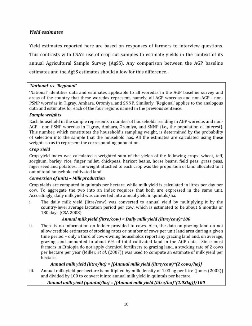
18
Yield estimates
Yield estimates reported here are based on responses of farmers to interview questions.
This contrasts with CSA’s use of crop cut samples to estimate yields in the context of its
annual Agricultural Sample Survey (AgSS). Any comparison between the AGP baseline
estimates and the AgSS estimates should allow for this difference.
‘National’ vs. ‘Regional’
‘National’ identifies data and estimates applicable to all woredas in the AGP baseline survey and areas of the country that these woredas represent, namely, all AGP woredas and non-AGP - non-PSNP woredas in Tigray, Amhara, Oromiya, and SNNP. Similarly, ‘Regional’ applies to the analogous data and estimates for each of the four regions named in the previous sentence.
Sample weights
Each household in the sample represents a number of households residing in AGP woredas and non-AGP - non-PSNP woredas in Tigray, Amhara, Oromiya, and SNNP (i.e., the population of interest). This number, which constitutes the household’s sampling weight, is determined by the probability of selection into the sample that the household has. All the estimates are calculated using these weights so as to represent the corresponding population.
Crop Yield
Crop yield index was calculated a weighted sum of the yields of the following crops: wheat, teff, sorghum, barley, rice, finger millet, chickpeas, haricot beans, horse beans, field peas, grass peas, niger seed and potatoes. The weight attached to each crop was the proportion of land allocated to it out of total household cultivated land.
Conversion of units – Milk production
Crop yields are computed in quintals per hectare, while milk yield is calculated in litres per day per cow. To aggregate the two into an index requires that both are expressed in the same unit. Accordingly, daily milk yield was converted into annual yield in quintals/ha.
i. The daily milk yield (litre/cow) was converted to annual yield by multiplying it by the country-level average lactation period per cow, which is estimated to be about 6 months or 180 days (CSA 2008)
Annual milk yield (litre/cow) = Daily milk yield (litre/cow)*180
ii. There is no information on fodder provided to cows. Also, the data on grazing land do not allow credible estimates of stocking rates or number of cows per unit land area during a given time period – only a third of cow-owning households report any grazing land and, on average, grazing land amounted to about 6% of total cultivated land in the AGP data . Since most farmers in Ethiopia do not apply chemical fertilizers to grazing land, a stocking rate of 2 cows per hectare per year (Miller, et al. (2007)) was used to compute an estimate of milk yield per hectare.
Annual milk yield (litre/ha) = [(Annual milk yield (litre/cow)*(2 cows/ha)]
iii. Annual milk yield per hectare is multiplied by milk density of 1.03 kg per litre (Jones (2002)) and divided by 100 to convert it into annual milk yield in quintals per hectare.
Annual milk yield (quintal/ha) = [(Annual milk yield (litre/ha)*(1.03kg)]/100

19
PDO 1 (National) – Agricultural yield1, by AGP Status
Group Category Quintal/ha
Total
All households 9.61
Female HHHs 8.48
Youth HHHs 9.78
AGP
All households 9.93
Female HHHs 9.44
Youth HHHs 10.28
Non AGP
All households 9.52
Female HHHs 8.17
Youth HHHs 9.63
Source: Authors’ calculations using data from the AGP Baseline Survey 2011.
Notes: ‘HHHs’ stands for ‘Household Heads’’. 1 Baseline agricultural yield is defined as a productivity index of the following agricultural commodity basket: crops (include wheat, teff, sorghum, barley, rice, finger millet, chickpeas, haricot beans, horse beans, field peas, grass peas, niger seed and potatoes), weighted 75%, and livestock products (only milk in the present case), weighted 25%.

20
PDO 1 (Regional) – Agricultural yield1, by region
Group Category Quintal/ha
Tigray
All households 7.64
Female HHHs 7.00 Youth HHHs 7.85
AGP HHHs 8.34
Female HHHs 7.23
Youth HHHs 8.68
Non-AGP 6.47 Female HHHs 6.63
Youth HHHs 6.40
Amhara
All households 11.21
Female HHHs 9.20
Youth HHHs 12.07 AGP HHHs 12.18
Female HHHs 11.39
Youth HHHs 12.43
Non-AGP 10.96
Female HHHs 8.75
Youth HHHs 11.98
Oromiya
All households 10.18
Female HHHs 8.91
Youth HHHs 10.27
AGP HHHs 10.68
Female HHHs 10.25
Youth HHHs 11.25
Non-AGP 10.02
Female HHHs 8.51
Youth HHHs 9.96
SNNP
All households 6.52
Female HHHs 6.48
Youth HHHs 5.78
AGP HHHs 4.87
Female HHHs 5.26
Youth HHHs 4.52 Non-AGP 6.87
Female HHHs 6.73
Youth HHHs 6.05 Source: Authors’ calculations using data from the AGP Baseline Survey 2011. Notes: HHHs’ stands for ‘Household Heads’’. 1 Baseline agricultural yield is defined as a productivity index of the following agricultural commodity basket: crops (include wheat, teff, sorghum, barley, rice, finger millet, chickpeas, haricot beans, horse beans, field peas, grass peas, niger seed and potatoes), weighted 75%, and livestock products (only milk in the present case), weighted 25%.
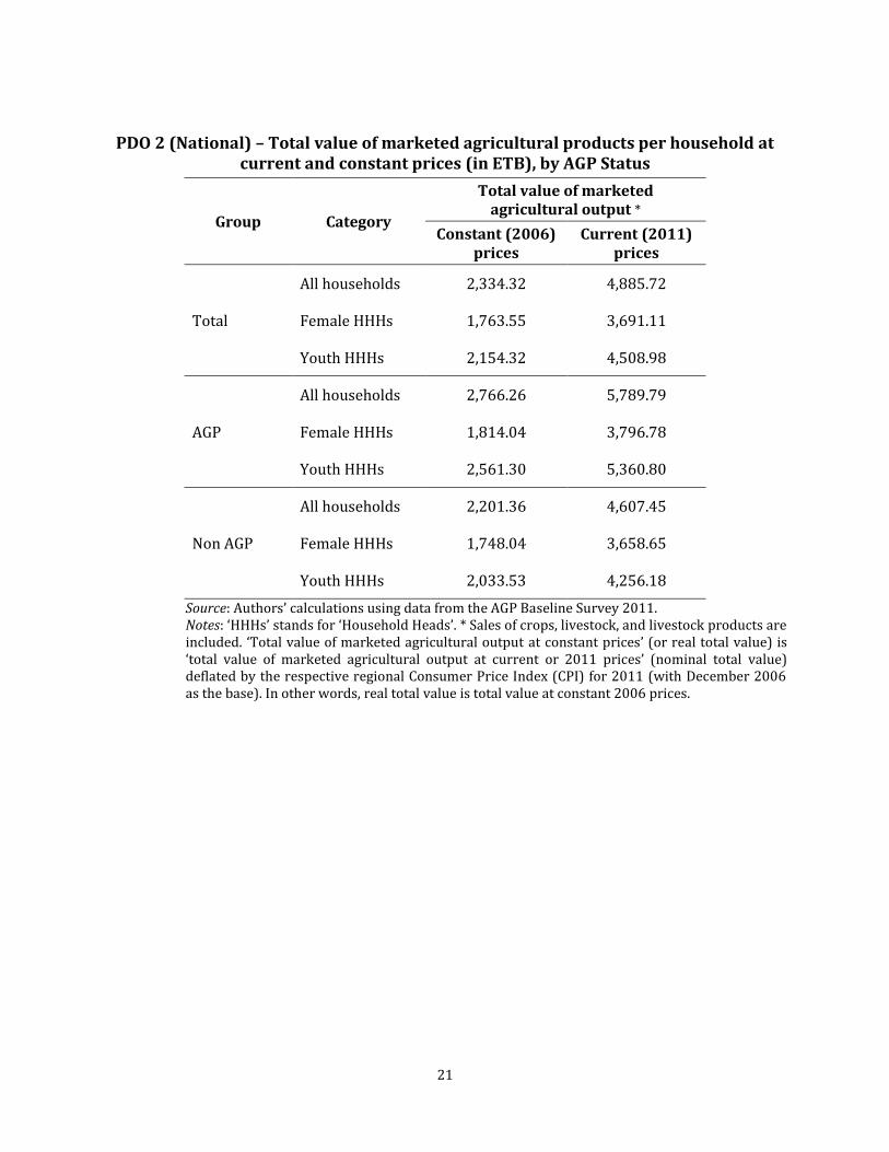
21
PDO 2 (National) – Total value of marketed agricultural products per household at current and constant prices (in ETB), by AGP Status
Group Category
Total value of marketed agricultural output *
Constant (2006) prices
Current (2011) prices
Total
All households 2,334.32 4,885.72
Female HHHs 1,763.55 3,691.11
Youth HHHs 2,154.32 4,508.98
AGP
All households 2,766.26 5,789.79
Female HHHs 1,814.04 3,796.78
Youth HHHs 2,561.30 5,360.80
Non AGP
All households 2,201.36 4,607.45
Female HHHs 1,748.04 3,658.65
Youth HHHs 2,033.53 4,256.18
Source: Authors’ calculations using data from the AGP Baseline Survey 2011. Notes: ‘HHHs’ stands for ‘Household Heads’. * Sales of crops, livestock, and livestock products are included. ‘Total value of marketed agricultural output at constant prices’ (or real total value) is ‘total value of marketed agricultural output at current or 2011 prices’ (nominal total value) deflated by the respective regional Consumer Price Index (CPI) for 2011 (with December 2006 as the base). In other words, real total value is total value at constant 2006 prices.

22
PDO 2 (Regional) – Total value of marketed agricultural products per household at current and constant prices (in ETB), by AGP Status and by Region
Group Category Total value of marketed agricultural output1
Constant (2006) prices Current (2011) prices
All households 1,451.78 3,492.97
Female HHHs 726.37 1,747.64
Youth HHHs 1,353.11 3,255.59
AGP HHHs 1,808.29 4,350.74
Tigray Female HHHs 869.99 2,093.19
Youth HHHs 1,694.97 4,078.09
Non-AGP HHHs 880.09 2,117.51
Female HHHs 501.26 1,206.04
Youth HHHs 753.35 1,812.56
All households 1,600.52 3,926.07
Female HHHs 879.54 2,157.50
Youth HHHs 1,655.76 4,061.58
AGP HHHs 2,543.06 6,238.12
Amhara Female HHHs 1,137.96 2,791.42
Youth HHHs 2,060.73 5,054.98
Non-AGP HHHs 1,316.18 3,228.58
Female HHHs 802.37 1,968.21
Youth HHHs 1,538.21 3,773.23
All households 2,163.49 5,728.92
Female HHHs 1,525.46 4,039.41
Youth HHHs 1,813.32 4,801.67
AGP HHHs 1,951.12 5,166.56
Oromiya Female HHHs 1,449.94 3,839.45
Youth HHHs 1,751.34 4,637.54
Non-AGP HHHs 2,232.09 5,910.57
Female HHHs 1,550.24 4,105.04
Youth HHHs 1,832.44 4,852.30
All households 1,684.12 4,547.13
Female HHHs 1,525.46 4,039.41
Youth HHHs 1,813.32 4,801.67
AGP HHHs 2,648.42 7,150.72
SNNP Female HHHs 2,045.46 5,522.75
Youth HHHs 2,889.09 7,800.53
Non-AGP HHHs 1,466.45 3,959.42
Female HHHs 1,718.82 4,640.82
Youth HHHs 1,432.58 3,867.96 Source: Authors’ calculations using data from the AGP Baseline Survey 2011. Notes: ‘HHHs’ stands for ‘Household Heads’. 1 Sales of crops, livestock, and livestock products are included. ‘Total value of marketed agricultural output at constant prices’ (or real total value) is ‘total value of marketed agricultural output at current or 2011 prices’ (nominal total value) deflated by the respective regional Consumer Price Index (CPI) for 2011 (with December 2006 as the base). In other words, real total value is total value at constant 2006 prices.

23
IO 1.1 (National) – Percentage of farmers satisfied with quality of extension services provided, by AGP Status
Group Category Level of
Satisfaction (%)
Percentage of households visited by
extension agents
Total
All households 91.9 26.97
Female HHHs 92.3 20.11
Youth HHHs 91.7 26.95
AGP
All households 92.0 27.90
Female HHHs 91.7 22.15
Youth HHHs 92.7 28.09
Non AGP
All households 91.9 26.68
Female HHHs 92.5 19.47
Youth HHHs 91.4 26.61 Source: Authors’ calculations using data from the AGP Baseline Survey 2011. Notes: ‘HHHs’ stands for ‘Household Heads’. The "level of satisfaction" is calculated using the response of households on how satisfied they were by the last expert visit. More specifically, it captures the fraction of households who replied ‘strongly agree’ or ‘agree’ to the question “The information provided (during the most recent visit) was satisfactory?” Interestingly, fewer households reported a visit in response to this question than when asked “How many times were you visited by an extension agent during the last main season?”
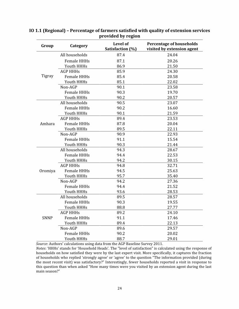
24
IO 1.1 (Regional) – Percentage of farmers satisfied with quality of extension services provided by region
Group Category Level of Satisfaction (%)
Percentage of households visited by extension agent
Tigray
All households 87.4 24.04
Female HHHs 87.1 20.26 Youth HHHs 86.9 21.50
AGP HHHs 85.9 24.30 Female HHHs 85.4 20.58 Youth HHHs 85.1 22.02
Non-AGP 90.1 23.58 Female HHHs 90.3 19.70 Youth HHHs 90.2 20.57
Amhara
All households 90.5 23.07 Female HHHs 90.2 16.60 Youth HHHs 90.1 21.59
AGP HHHs 89.4 23.53 Female HHHs 87.8 20.04 Youth HHHs 89.5 22.11
Non-AGP 90.9 22.93 Female HHHs 91.1 15.54 Youth HHHs 90.3 21.44
Oromiya
All households 94.3 28.67 Female HHHs 94.4 22.53 Youth HHHs 94.2 30.15
AGP HHHs 94.8 32.71 Female HHHs 94.5 25.63 Youth HHHs 95.7 35.40
Non-AGP 94.2 27.36 Female HHHs 94.4 21.52 Youth HHHs 93.6 28.53
SNNP
All households 89.5 28.57 Female HHHs 90.3 19.55 Youth HHHs 88.8 27.77
AGP HHHs 89.2 24.10 Female HHHs 91.1 17.46 Youth HHHs 89.4 22.13
Non-AGP 89.6 29.57 Female HHHs 90.2 20.02 Youth HHHs 88.7 29.01
Source: Authors’ calculations using data from the AGP Baseline Survey 2011. Notes: ‘HHHs’ stands for ‘Household Heads’. The "level of satisfaction" is calculated using the response of households on how satisfied they were by the last expert visit. More specifically, it captures the fraction of households who replied ‘strongly agree’ or ‘agree’ to the question “The information provided (during the most recent visit) was satisfactory?” Interestingly, fewer households reported a visit in response to this question than when asked “How many times were you visited by an extension agent during the last main season?”

25
IO 2.3 (National) – Area under irrigation (level and per cent of cultivated land) by AGP Status
Total land under
irrigation (hectare)
Total land size cultivated by
households (ha)
Percentage of irrigated land
Total
All households 179,645 11,690,413 1.54
Female HHHs 23,339 2,767,548 0.84
Youth HHHs 69,765 3,935,530 1.77
AGP
All households 70,603 3,057,938 2.31
Female HHHs 15,094 660,839 2.28
Youth HHHs 20,635 1,016,151 2.03
Non AGP
All households 109,042 8,632,241 1.26
Female HHHs 8,244 2,106,710 0.39
Youth HHHs 49,130 2,919,379 1.68
Source: Authors’ calculations using data from the AGP Baseline Survey 2011. Notes: ‘HHHs’ stands for ‘Household Heads’.
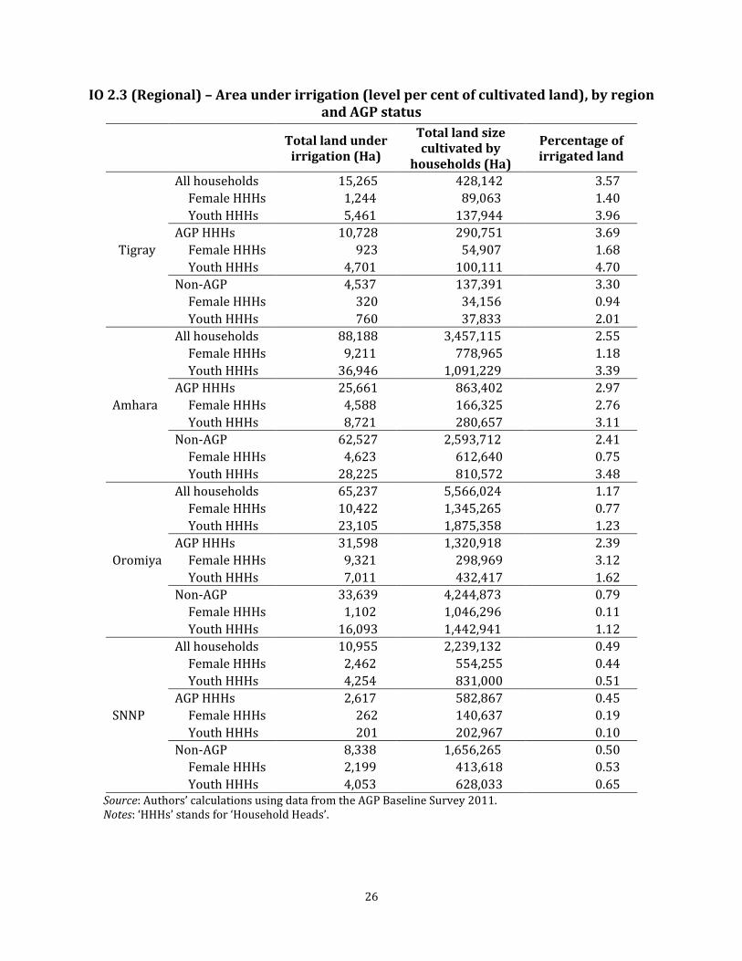
26
IO 2.3 (Regional) – Area under irrigation (level per cent of cultivated land), by region and AGP status
Total land under
irrigation (Ha)
Total land size cultivated by
households (Ha)
Percentage of irrigated land
Tigray
All households 15,265 428,142 3.57
Female HHHs 1,244 89,063 1.40
Youth HHHs 5,461 137,944 3.96
AGP HHHs 10,728 290,751 3.69
Female HHHs 923 54,907 1.68
Youth HHHs 4,701 100,111 4.70
Non-AGP 4,537 137,391 3.30
Female HHHs 320 34,156 0.94
Youth HHHs 760 37,833 2.01
Amhara
All households 88,188 3,457,115 2.55
Female HHHs 9,211 778,965 1.18
Youth HHHs 36,946 1,091,229 3.39
AGP HHHs 25,661 863,402 2.97
Female HHHs 4,588 166,325 2.76
Youth HHHs 8,721 280,657 3.11
Non-AGP 62,527 2,593,712 2.41
Female HHHs 4,623 612,640 0.75
Youth HHHs 28,225 810,572 3.48
Oromiya
All households 65,237 5,566,024 1.17
Female HHHs 10,422 1,345,265 0.77
Youth HHHs 23,105 1,875,358 1.23
AGP HHHs 31,598 1,320,918 2.39
Female HHHs 9,321 298,969 3.12
Youth HHHs 7,011 432,417 1.62
Non-AGP 33,639 4,244,873 0.79
Female HHHs 1,102 1,046,296 0.11
Youth HHHs 16,093 1,442,941 1.12
SNNP
All households 10,955 2,239,132 0.49
Female HHHs 2,462 554,255 0.44
Youth HHHs 4,254 831,000 0.51
AGP HHHs 2,617 582,867 0.45
Female HHHs 262 140,637 0.19
Youth HHHs 201 202,967 0.10
Non-AGP 8,338 1,656,265 0.50
Female HHHs 2,199 413,618 0.53
Youth HHHs 4,053 628,033 0.65 Source: Authors’ calculations using data from the AGP Baseline Survey 2011. Notes: ‘HHHs’ stands for ‘Household Heads’.

27
IO 2.4 (National) – Percentage of households practicing soil conservation and water harvesting, by AGP status
Group Category Soil
conservation (%)
Water harvesting
(%)
Total
All households 72.4 15.3
Female HHHs 66.4 10.6
Youth HHHs 70.8 15.8
AGP
All households 71.0 19.8
Female HHHs 66.2 15.1
Youth HHHs 71.1 19.1
Non AGP
All households 72.8 13.9
Female HHHs 66.4 9.2
Youth HHHs 70.7 14.9 Source: Authors’ calculations using data from the AGP Baseline Survey 2011. Notes: ‘HHHs’ stands for ‘Household Heads’. The three most common types of soil conservation activities adopted by households are fanya juu (34.7 percent), stone bunds (29.1 percent) and soil bunds (22.2 percent). Fanya Juu is an embankment along the contour which is made of soil or stones, with a purpose of conserving soil moisture and controlling erosion.

28
IO 2.4 (Regional) – Percentage of households practicing soil conservation and water harvesting, by region.
Group Category Soil
conservation Water
harvesting
Tigray
All households 84.6 32.5
Female HHHs 80.5 23.4
Youth HHHs 86.7 31.6
AGP HHHs 80.1 33.8
Female HHHs 73.5 23.0
Youth HHHs 82.8 33.3
Non-AGP 92.3 30.3
Female HHHs 92.2 24.2
Youth HHHs 93.6 28.6
Amhara
All households 88.2 15.0
Female HHHs 81.2 9.7
Youth HHHs 87.9 13.0
AGP HHHs 81.3 12.4
Female HHHs 75.5 8.3
Youth HHHs 80.9 12.4
Non-AGP 90.3 15.7
Female HHHs 83.0 10.1
Youth HHHs 89.9 13.2
Oromiya
All households 76.1 17.0
Female HHHs 70.2 12.3
Youth HHHs 73.3 19.1
AGP HHHs 80.1 26.7
Female HHHs 75.5 22.4
Youth HHHs 80.3 25.7
Non-AGP 74.8 13.9
Female HHHs 68.5 9.0
Youth HHHs 71.1 17.1
SNNP
All households 47.5 10.5
Female HHHs 42.4 7.0
Youth HHHs 46.4 11.4
AGP HHHs 32.2 7.7
Female HHHs 28.5 3.7
Youth HHHs 32.0 7.4
Non-AGP 50.9 11.1
Female HHHs 45.4 7.7
Youth HHHs 49.6 12.3 Source: Authors’ calculations using data from the AGP Baseline Survey 2011. Notes: ‘HHHs’ stands for ‘Household Heads’. The three most common types of soil conservation activities adopted by households are fanya juu (34.7 percent), stone bunds (29.1 percent) and soil bunds (22.2 percent). Fanya Juu is an embankment along the contour which is made of soil or stones, with a purpose of conserving soil moisture and controlling erosion.

29
IO.2.5.Community level information on travel time to the nearest market centre (with a population of 50,000 or more) in hours
Category Travel time to the nearest
market centre
National
All woredas 3.1
AGP woredas 1.9
Non-AGP woredas 3.5
Tigray
All woredas 1.9
AGP woredas 2.0
Non- AGP woredas 1.5
Amhara
All woredas 4.5
AGP woredas 2.5
Non- AGP woredas 5.1
Oromiya
All woredas 2.6
AGP woredas 1.3
Non- AGP woredas 2.9
SNNP
All woredas 2.6
AGP woredas 2.4
Non- AGP woredas 2.7
Source: Authors’ calculations using data from the AGP Baseline Survey 2011. Notes: Household level data on travel times were not collected. Data on the household-level costs of moving products to and from markets were collected, instead (see Tables ES.4-ES.5 below). More disaggregated travel time data will be coleected in the next survey round.

30
Annex to the Executive Summary
Table ES.1 – Percentage of Kebeles with farmer organizations and the services they provide, by AGP status (related to IO 1.2)
Community level variables Non-AGP AGP Total
Rural savings and credit cooperative in PA 31.2 34.8 32.1
There are restrictions on who can join the cooperatives 66.7 78.2 69.5
Sell/distribute improved seeds or hybrids 19.4 30.2 21.8
Provide agricultural credit 22.9 31.9 25
Supply fertilizer 29.1 32.8 29.9
Village saving and loan association in the PA 16 21.9 17.4
There are restrictions on who can join the cooperatives 55.9 72.7 60.1
Sell/distribute improved seeds or hybrids 10.5 18.1 12.3
Provide agricultural credit 15.4 23.8 17.3
Supply fertilizer 12 19.1 13.7
Producer association in the PA 23.8 16.6 22.1
There are restrictions on who can join the cooperatives 64.8 64.2 64.7
Sell/distribute improved seeds or hybrids 33.3 24 31.2
Provide agricultural credit 7 18.7 9.7
Supply fertilizer 36.7 25.7 34.1 Source: Authors’ calculations using data from the AGP Baseline Survey 2011
Table ES.2 – Percentage of households using chemical fertilizer, improved seed and irrigation by AGP Status (related to IO 1.3)
Group Category Chemical fertilizer
users
Improved seed users
Irrigation
Total
All households 57.5 22.5 4.2
Female HHHs 48.7 16.7 2.9
Youth HHHs 57.7 22.1 4.0
AGP
All households 62.2 22.1 7.8
Female HHHs 52.7 18.0 6.3
Youth HHHs 62.0 22.5 7.4
Non AGP
All households 62.2 22.6 3.1
Female HHHs 47.5 16.3 1.9
Youth HHHs 56.0 22.0 2.9 Source: Authors’ calculations using data from the AGP Baseline Survey 2011. Notes: HHHs and HHs stand respectively for ‘Household Heads’ and ‘Households’.

31
Table ES.3 – Percentage of households using chemical fertilizer, improved seed and irrigation (related to IO 1.3)
Group Category Chemical fertilizer users Improved seed users Irrigation
All households 56.8 18.4 8.5
Female HHHs 48.0 11.8 7.0
Youth HHHs 53.0 18.9 8.4
AGP HHHs 44.0 12.0 7.4
Tigray Female HHHs 35.4 6.0 7.3
Youth HHHs 40.3 12.0 7.0
Non-AGP 78.0 29.0 10.4
Female HHHs 69.0 20.7 6.5
Youth HHHs 75.2 31.0 10.8
Amhara
All households 59.0 33.8 7.2
Female HHHs 47.0 25.8 4.3
Youth HHHs 58.0 33.8 6.7
AGP HHHs 65.8 45.9 12.3
Female HHHs 52.2 36.4 8.7
Youth HHHs 67.1 46.7 11.3
Non-AGP 56.8 30.0 5.8
Female HHHs 45.0 22.6 3.0
Youth HHHs 55.7 30.0 5.3
Oromiya
All households 66.0 21.5 3.4
Female HHHs 57.0 16.2 2.9
Youth HHHs 69.0 20.7 3.6
AGP HHHs 73.6 13.2 8.1
Female HHHs 65.0 12.5 7.5
Youth HHHs 75.0 14.0 8.1
Non-AGP 64.0 24.0 1.9
Female HHHs 54.5 17.0 1.5
Youth HHHs 66.7 22.6 2.3
SNNP
All households 41.0 13.1 1.8
Female HHHs 36.0 9.4 1.1
Youth HHHs 39.0 13.2 1.4
AGP HHHs 38.0 15.0 1.2
Female HHHs 31.0 12.7 0.7
Youth HHHs 34.7 14.0 0.9
Non-AGP 41.0 12.6 2.0
Female HHHs 37.5 8.6 1.2
Youth HHHs 40.0 12.9 1.5 Source: Authors’ calculations using data from the AGP Baseline Survey 2011 Notes: HHHs and HHs stand respectively for ‘Household Heads’ and ‘Households’.

32
Table ES.4 – Transport Cost (Birr per quintal) to the nearest market in …
Group Category Respondents’
village Local market
town
Total
All households 3.26 20.95
Female HHHs 3.3 17.3
Youth HHHs 4.63 28.42
AGP
All households 4.3 14.67
Female HHHs 6.94 8.98
Youth HHHs 4.79 16.5
Non AGP
All households 2.88 22.95
Female HHHs 1.98 19.88
Youth HHHs 4.57 32.06
Source: Authors’ calculations using data from the AGP Baseline Survey 2011. Notes: HHHs and HHs stand respectively for ‘Household Heads’ and ‘Households’.
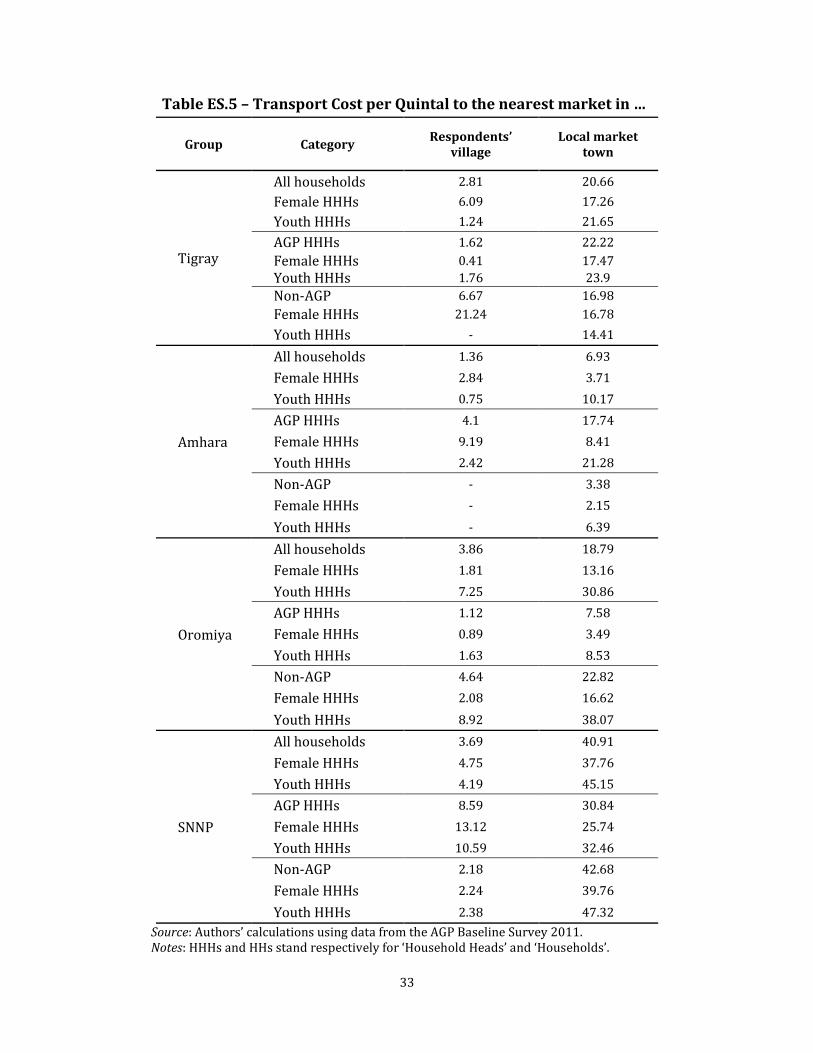
33
Table ES.5 – Transport Cost per Quintal to the nearest market in …
Group Category Respondents’
village Local market
town
Tigray
All households 2.81 20.66
Female HHHs 6.09 17.26
Youth HHHs 1.24 21.65
AGP HHHs 1.62 22.22
Female HHHs 0.41 17.47
Youth HHHs 1.76 23.9
Non-AGP 6.67 16.98
Female HHHs 21.24 16.78
Youth HHHs - 14.41
Amhara
All households 1.36 6.93
Female HHHs 2.84 3.71
Youth HHHs 0.75 10.17
AGP HHHs 4.1 17.74
Female HHHs 9.19 8.41
Youth HHHs 2.42 21.28
Non-AGP - 3.38
Female HHHs - 2.15
Youth HHHs - 6.39
Oromiya
All households 3.86 18.79
Female HHHs 1.81 13.16
Youth HHHs 7.25 30.86
AGP HHHs 1.12 7.58
Female HHHs 0.89 3.49
Youth HHHs 1.63 8.53
Non-AGP 4.64 22.82
Female HHHs 2.08 16.62
Youth HHHs 8.92 38.07
SNNP
All households 3.69 40.91
Female HHHs 4.75 37.76
Youth HHHs 4.19 45.15
AGP HHHs 8.59 30.84
Female HHHs 13.12 25.74
Youth HHHs 10.59 32.46
Non-AGP 2.18 42.68
Female HHHs 2.24 39.76
Youth HHHs 2.38 47.32
Source: Authors’ calculations using data from the AGP Baseline Survey 2011. Notes: HHHs and HHs stand respectively for ‘Household Heads’ and ‘Households’.
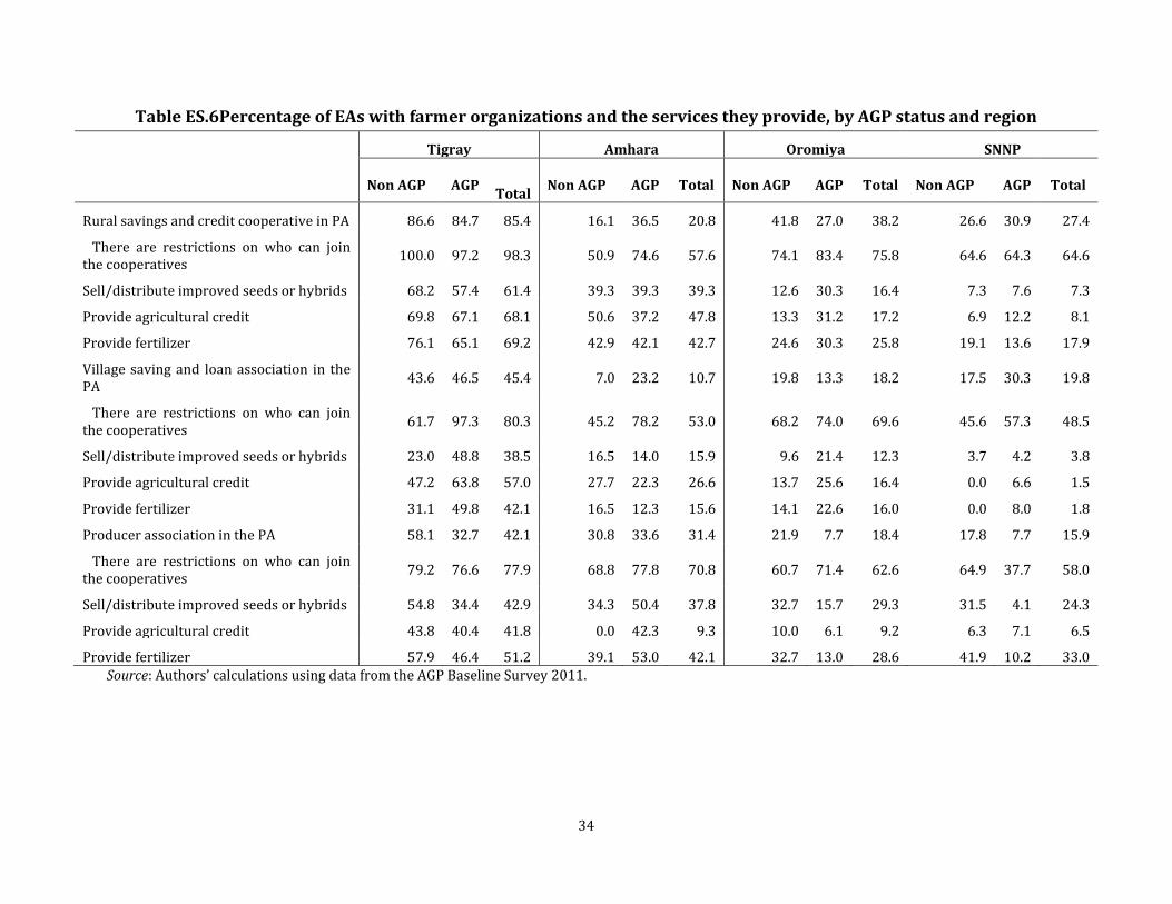
34
Table ES.6Percentage of EAs with farmer organizations and the services they provide, by AGP status and region
Tigray Amhara Oromiya SNNP
Non AGP AGP
Total
Non AGP AGP Total Non AGP AGP Total Non AGP AGP Total
Rural savings and credit cooperative in PA 86.6 84.7 85.4 16.1 36.5 20.8 41.8 27.0 38.2 26.6 30.9 27.4
There are restrictions on who can join the cooperatives
100.0 97.2 98.3 50.9 74.6 57.6 74.1 83.4 75.8 64.6 64.3 64.6
Sell/distribute improved seeds or hybrids 68.2 57.4 61.4 39.3 39.3 39.3 12.6 30.3 16.4 7.3 7.6 7.3
Provide agricultural credit 69.8 67.1 68.1 50.6 37.2 47.8 13.3 31.2 17.2 6.9 12.2 8.1
Provide fertilizer 76.1 65.1 69.2 42.9 42.1 42.7 24.6 30.3 25.8 19.1 13.6 17.9
Village saving and loan association in the PA
43.6 46.5 45.4 7.0 23.2 10.7 19.8 13.3 18.2 17.5 30.3 19.8
There are restrictions on who can join the cooperatives
61.7 97.3 80.3 45.2 78.2 53.0 68.2 74.0 69.6 45.6 57.3 48.5
Sell/distribute improved seeds or hybrids 23.0 48.8 38.5 16.5 14.0 15.9 9.6 21.4 12.3 3.7 4.2 3.8
Provide agricultural credit 47.2 63.8 57.0 27.7 22.3 26.6 13.7 25.6 16.4 0.0 6.6 1.5
Provide fertilizer 31.1 49.8 42.1 16.5 12.3 15.6 14.1 22.6 16.0 0.0 8.0 1.8
Producer association in the PA 58.1 32.7 42.1 30.8 33.6 31.4 21.9 7.7 18.4 17.8 7.7 15.9
There are restrictions on who can join the cooperatives
79.2 76.6 77.9 68.8 77.8 70.8 60.7 71.4 62.6 64.9 37.7 58.0
Sell/distribute improved seeds or hybrids 54.8 34.4 42.9 34.3 50.4 37.8 32.7 15.7 29.3 31.5 4.1 24.3
Provide agricultural credit 43.8 40.4 41.8 0.0 42.3 9.3 10.0 6.1 9.2 6.3 7.1 6.5
Provide fertilizer 57.9 46.4 51.2 39.1 53.0 42.1 32.7 13.0 28.6 41.9 10.2 33.0 Source: Authors’ calculations using data from the AGP Baseline Survey 2011.

35
Table ES.7 Distance to the nearest town and type of first important road, by region and AGP status.
Region Category
Distance to nearest large town (KMs)
First important road made of (%)
Mean Median SD Concrete Stones Dirt Others
National
All woredas 13.9 10 12.2 11.0 18.8 55.8 14.4
AGP woredas 14.4 10 13.7 13.4 21.6 49.0 16.0
Non-AGP woredas 12.7 10 8.5 6.1 13.3 69.4 11.2
Tigray
All woredas 15.7 14 11.6 16.7 3.3 73.3 6.7
AGP woredas 16.0 14 13.0 22.0 0.0 70.7 7.3
Non-AGP woredas 14.9 14 7.9 5.3 10.5 78.9 5.3
Amhara
All woredas 16.6 12 12.3 5.6 22.2 48.6 23.6
AGP woredas 17.1 12 13.2 8.0 28.0 40.0 24.0
Non-AGP woredas 15.5 14 10.2 0.0 9.1 68.2 22.7
Oromiya
All woredas 12.6 10 9.7 13.9 26.6 43.0 16.5
AGP woredas 12.2 10 10.4 13.5 30.8 36.5 19.2
Non-AGP woredas 13.4 12 8.2 14.8 18.5 55.6 11.1
SNNP
All woredas 11.1 7 14.1 8.6 19.8 61.7 9.9
AGP woredas 12.7 8 17.1 11.8 23.5 52.9 11.8
Non-AGP woredas 8.2 7 5.5 3.3 13.3 76.7 6.7
Source: Authors’ calculations using data from the AGP Baseline Survey, 2011.
Table ES.8 Accessibility of the first most important road, by region and AGP status.
Region Category
Accessibility of first important road during rainy season (%)
Accessibility of first important road during dry season (%)
Any vehicle
Trucks and
buses
Mini-bus
Carts or animals
Only walking
Any vehicle
Trucks and
buses
Mini-bus
Carts or animals
Only walking
National
All woredas 30.6 6.2 2.4 13.4 47.4 45.9 7.9 8.9 10.3 27.1
AGP woredas 34.4 5.7 2.6 13.0 44.3 50.5 6.8 7.8 9.4 25.5
Non-AGP woredas 23.2 7.1 2.0 14.1 53.5 37.0 10.0 11.0 12.0 30.0
Tigray
All woredas 38.6 10.5 7.0 3.5 40.4 58.6 12.1 17.2 0.0 12.1
AGP woredas 44.7 5.3 7.9 2.6 39.5 64.1 10.3 12.8 0.0 12.8
Non-AGP woredas 26.3 21.1 5.3 5.3 42.1 47.4 15.8 26.3 0.0 10.5
Amhara
All woredas 31.1 1.4 1.4 8.1 58.1 51.4 5.4 8.1 6.8 28.4
AGP woredas 38.0 2.0 2.0 8.0 50.0 60.0 4.0 6.0 4.0 26.0
Non-AGP woredas 16.7 0.0 0.0 8.3 75.0 33.3 8.3 12.5 12.5 33.3
Oromiya
All woredas 35.0 8.8 0.0 16.3 40.0 38.8 10.0 0.0 18.8 32.5
AGP woredas 37.7 9.4 0.0 13.2 39.6 43.4 7.5 0.0 17.0 32.1
Non-AGP woredas 29.6 7.4 0.0 22.2 40.7 29.6 14.8 0.0 22.2 33.3
SNNP
All woredas 20.0 5.0 2.5 22.5 50.0 38.8 5.0 12.5 12.5 31.3
AGP woredas 19.6 5.9 2.0 25.5 47.1 38.0 6.0 14.0 14.0 28.0
Non-AGP woredas 20.7 3.4 3.4 17.2 55.2 40.0 3.3 10.0 10.0 36.7
Source: Authors’ calculations using data from the AGP Baseline Survey 2011.
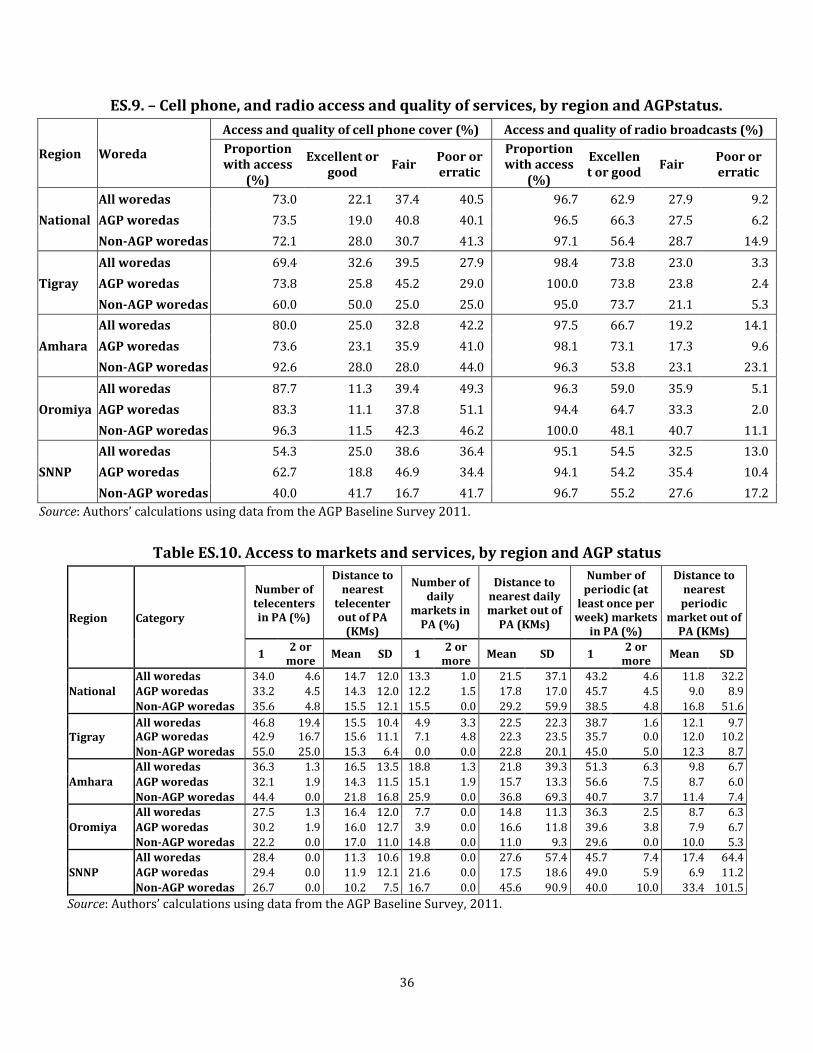
36
ES.9. – Cell phone, and radio access and quality of services, by region and AGPstatus.
Region Woreda
Access and quality of cell phone cover (%) Access and quality of radio broadcasts (%)
Proportion with access
(%)
Excellent or good
Fair Poor or erratic
Proportion with access
(%)
Excellent or good
Fair Poor or erratic
National
All woredas 73.0 22.1 37.4 40.5 96.7 62.9 27.9 9.2
AGP woredas 73.5 19.0 40.8 40.1 96.5 66.3 27.5 6.2
Non-AGP woredas 72.1 28.0 30.7 41.3 97.1 56.4 28.7 14.9
Tigray
All woredas 69.4 32.6 39.5 27.9 98.4 73.8 23.0 3.3
AGP woredas 73.8 25.8 45.2 29.0 100.0 73.8 23.8 2.4
Non-AGP woredas 60.0 50.0 25.0 25.0 95.0 73.7 21.1 5.3
Amhara
All woredas 80.0 25.0 32.8 42.2 97.5 66.7 19.2 14.1
AGP woredas 73.6 23.1 35.9 41.0 98.1 73.1 17.3 9.6
Non-AGP woredas 92.6 28.0 28.0 44.0 96.3 53.8 23.1 23.1
Oromiya
All woredas 87.7 11.3 39.4 49.3 96.3 59.0 35.9 5.1
AGP woredas 83.3 11.1 37.8 51.1 94.4 64.7 33.3 2.0
Non-AGP woredas 96.3 11.5 42.3 46.2 100.0 48.1 40.7 11.1
SNNP
All woredas 54.3 25.0 38.6 36.4 95.1 54.5 32.5 13.0
AGP woredas 62.7 18.8 46.9 34.4 94.1 54.2 35.4 10.4
Non-AGP woredas 40.0 41.7 16.7 41.7 96.7 55.2 27.6 17.2
Source: Authors’ calculations using data from the AGP Baseline Survey 2011.
Table ES.10. Access to markets and services, by region and AGP status
Region Category
Number of telecenters in PA (%)
Distance to nearest
telecenter out of PA
(KMs)
Number of daily
markets in PA (%)
Distance to nearest daily market out of
PA (KMs)
Number of periodic (at
least once per week) markets
in PA (%)
Distance to nearest periodic
market out of PA (KMs)
1 2 or
more Mean SD 1
2 or more
Mean SD 1 2 or
more Mean SD
National
All woredas 34.0 4.6 14.7 12.0 13.3 1.0 21.5 37.1 43.2 4.6 11.8 32.2
AGP woredas 33.2 4.5 14.3 12.0 12.2 1.5 17.8 17.0 45.7 4.5 9.0 8.9
Non-AGP woredas 35.6 4.8 15.5 12.1 15.5 0.0 29.2 59.9 38.5 4.8 16.8 51.6
Tigray All woredas 46.8 19.4 15.5 10.4 4.9 3.3 22.5 22.3 38.7 1.6 12.1 9.7 AGP woredas 42.9 16.7 15.6 11.1 7.1 4.8 22.3 23.5 35.7 0.0 12.0 10.2
Non-AGP woredas 55.0 25.0 15.3 6.4 0.0 0.0 22.8 20.1 45.0 5.0 12.3 8.7
Amhara
All woredas 36.3 1.3 16.5 13.5 18.8 1.3 21.8 39.3 51.3 6.3 9.8 6.7
AGP woredas 32.1 1.9 14.3 11.5 15.1 1.9 15.7 13.3 56.6 7.5 8.7 6.0
Non-AGP woredas 44.4 0.0 21.8 16.8 25.9 0.0 36.8 69.3 40.7 3.7 11.4 7.4
Oromiya
All woredas 27.5 1.3 16.4 12.0 7.7 0.0 14.8 11.3 36.3 2.5 8.7 6.3
AGP woredas 30.2 1.9 16.0 12.7 3.9 0.0 16.6 11.8 39.6 3.8 7.9 6.7
Non-AGP woredas 22.2 0.0 17.0 11.0 14.8 0.0 11.0 9.3 29.6 0.0 10.0 5.3
SNNP
All woredas 28.4 0.0 11.3 10.6 19.8 0.0 27.6 57.4 45.7 7.4 17.4 64.4
AGP woredas 29.4 0.0 11.9 12.1 21.6 0.0 17.5 18.6 49.0 5.9 6.9 11.2
Non-AGP woredas 26.7 0.0 10.2 7.5 16.7 0.0 45.6 90.9 40.0 10.0 33.4 101.5
Source: Authors’ calculations using data from the AGP Baseline Survey, 2011.

37
Table ES.11. Yield in quintals for major cereals, pulses and oil seeds by AGP status and egion
Group Category Statistic Teff Barley Wheat Maize Sorghum Pulses Oil
Seeds
National All HHHs
Mean 9.4 14.7 14.6 17.2 11.5 10.9 5.1
Median 6.7 9.6 10.0 12.0 8.0 6.7 4.0
SD 9.0 14.8 14.4 17.4 10.4 14.2 5.8
AGP woredas
All HHHs
Mean 9.8 14.0 15.1 16.0 13.0 12.6 7.0
Median 8.0 10.0 10.7 10.0 9.3 8.0 4.0
SD 9.1 14.0 14.5 17.0 12.9 14.1 9.0
Non-AGP woredas
All HHHs
Mean 9.2 14.9 14.4 17.6 10.9 10.4 4.4
Median 6.0 9.5 9.6 12.0 8.0 6.0 3.8
SD 8.9 15.0 14.3 17.5 9.1 14.2 3.5
Tigray
All Households
Mean 7.7 10.8 11.6 10.5 10.9 9.1 4.6
Median 6.0 8.0 8.3 6.9 8.0 6.7 3.2
SD 7.1 8.3 9.4 12.7 10.1 15.0 6.2
AGP Households
Mean 7.9 11.2 12.5 11.0 11.9 8.4 4.8
Median 6.0 8.0 10.0 6.7 9.3 6.4 3.2
SD 6.9 9.2 10.0 13.4 10.8 7.8 6.7
Non-AGP Households
Mean 7.4 10.3 10.8 9.8 7.5 10.2 3.8
Median 5.9 8.0 8.0 7.2 6.0 8.0 2.8
SD 7.4 7.2 8.7 11.5 5.9 21.8 2.8
Amhara
All Households
Mean 12.1 16.8 16.5 24.7 11.6 12.5 6.6
Median 8.0 8.7 9.3 15.0 9.0 6.0 4.0
SD 11.0 19.0 18.5 24.4 9.4 18.1 8.3
AGP Households
Mean 11.2 16.0 21.1 20.7 13.0 13.7 8.5
Median 8.0 10.7 14.0 15.0 9.6 8.0 4.8
SD 10.8 15.6 21.1 19.2 13.3 19.0 11.0
Non-AGP Households
Mean 12.4 17.0 15.9 27.1 11.1 12.4 5.3
Median 8.4 8.0 8.4 16.0 9.0 6.0 3.2
SD 11.0 19.5 18.1 26.7 7.8 17.9 5.6
Oromiya
All Households
Mean 8.4 15.9 14.7 17.5 12.2 11.5 4.6
Median 6.7 12.0 11.2 13.7 8.4 8.0 4.0
SD 7.1 12.9 11.9 14.6 11.6 11.1 4.1
AGP Households
Mean 9.8 16.0 15.2 17.2 15.0 14.0 6.8
Median 8.0 12.0 11.3 11.2 11.2 10.0 4.0
SD 8.1 14.7 13.2 17.2 14.3 12.8 7.8
Non-AGP Households
Mean 7.5 15.8 14.4 17.6 11.2 10.4 4.0
Median 6.0 12.0 11.2 14.0 8.0 8.0 3.8
SD 6.3 12.3 11.2 13.9 10.4 10.1 2.4
SNNP
All Households
Mean 5.5 7.5 10.5 10.7 9.0 6.9 5.2
Median 4.0 5.6 8.0 7.5 8.0 4.2 3.8
SD 5.4 7.2 10.9 11.9 7.0 10.4 3.5
AGP Households
Mean 4.7 7.8 7.2 7.2 6.2 6.0 3.8
Median 2.8 5.0 5.0 5.0 5.0 4.0 3.5
SD 5.3 8.4 6.7 7.4 5.3 8.1 2.2
Non-AGP Households
Mean 5.6 7.4 11.2 11.5 9.6 7.0 6.1
Median 4.0 5.6 8.0 8.0 8.0 4.2 6.3
SD 5.4 6.8 11.5 12.7 7.1 10.7 3.9
Source: Authors’ calculations using data from the AGP Baseline Survey 2011. Note: ‘SD’ stands for ‘Standard Deviation’.

38
Table ES.12. Milk yield in litre per cow per day by AGP status and region
Group Category Milk yield
(litres/cow/day)
Mean SD
National All Households 0.95 0.7 AGP Households All Households 0.93 0.73 Non-AGP Households All Households 0.96 0.69
Tigray
All Households 0.94 0.83
AGP Households 1.02 0.87
Non-AGP Households 0.79 0.72
Amhara
All Households 0.97 0.75
AGP Households 0.75 0.45
Non-AGP Households 1.10 0.86
Oromiya
All Households 0.90 0.64
AGP Households 0.94 0.76
Non-AGP Households 0.89 0.59
SNNP
All Households 1.03 0.75
AGP Households 1.20 1.07
Non-AGP Households 0.98 0.62
Source: Authors’ calculations using data from the AGP Baseline Survey 2011.
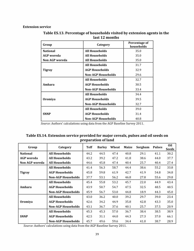
39
Extension service
Table ES.13. Percentage of households visited by extension agents in the last 12 months
Group Category Percentage of
households
National All Households 35.0
AGP woreda All Households 35.0
Non AGP woreda All Households 35.0
Tigray
All Households 31.7
AGP Households 32.9
Non-AGP Households 29.6
Amhara
All Households 32.7
AGP Households 30.5
Non-AGP Households 33.4
Oromiya
All Households 34.4
AGP Households 39.5
Non-AGP Households 32.7
SNNP
All Households 39.0
AGP Households 31.4
Non-AGP Households 40.8
Source: Authors’ calculations using data from the AGP Baseline Survey 2011.
Table ES.14. Extension service provided for major cereals, pulses and oil seeds on preparation of land
Group Category Teff Barley Wheat Maize Sorghum Pulses Oil
Seeds
National All Households 44.2 44.5 47.4 40.8 29.1 41.1 30.2
AGP woreda All Households 43.2 39.2 47.2 41.8 38.6 44.0 37.7
Non AGP woreda All Households 44.6 45.8 47.4 40.4 25.7 40.4 27.4
Tigray
All Households 41.4 56.3 58.7 44.4 38.6 55.2 33.8
AGP Households 45.8 59.8 61.9 42.7 41.9 54.8 34.8
Non-AGP Households 37.7 53.1 56.2 46.8 27.8 55.6 29.8
Amhara
All Households 45.4 55.8 53.2 45.7 22.0 44.9 43.4
AGP Households 43.9 50.7 54.7 47.5 32.5 48.5 40.5
Non-AGP Households 45.9 56.7 53.0 44.8 18.9 44.3 45.0
Oromiya
All Households 43.0 36.2 40.0 39.2 29.7 39.0 23.4
AGP Households 42.6 34.2 44.9 35.8 42.8 43.3 35.0
Non-AGP Households 43.1 36.7 37.6 40.1 25.7 37.5 20.9
SNNP
All Households 45.3 45.3 57.0 36.7 38.4 38.5 38.9
AGP Households 42.5 31.1 44.0 44.3 27.3 37.0 66.1
Non-AGP Households 45.7 49.6 59.6 34.4 41.0 38.7 28.9
Source: Authors’ calculations using data from the AGP Baseline Survey 2011.

40
Table ES.15. Extension service provided for major cereals, pulses and oil seeds on methods of planting
Group Category Teff Barley Wheat Maize Sorghum Pulses Oil
Seeds
National All Households 44.6 44.4 47.5 42.4 28.9 41.6 30.7
AGP woreda All Households 42.3 37.8 48.0 43.2 39.6 43.6 38.0
Non AGP woreda All Households 45.5 46.1 47.4 42.1 25.1 41.1 28.0
Tigray
All Households 41.7 57.4 59.4 47.3 43.0 53.6 40.7
AGP Households 47.1 62.3 63.7 48.4 47.3 52.5 42.4
Non-AGP Households 37.1 52.8 55.9 45.8 28.7 55.0 33.4
Amhara
All Households 46.5 56.5 52.6 50.1 21.0 45.9 44.4
AGP Households 44.4 49.1 55.2 49.3 31.9 47.4 40.2
Non-AGP Households 47.2 57.7 52.2 50.5 17.8 45.6 46.7
Oromiya
All Households 43.2 36.0 40.3 39.8 29.3 39.2 22.9
AGP Households 40.6 31.4 45.2 36.2 43.0 43.3 32.5
Non-AGP Households 44.6 37.2 37.9 40.8 25.1 37.8 20.9
SNNP
All Households 44.3 43.8 58.0 36.3 38.0 38.7 37.8
AGP Households 41.7 31.5 46.7 45.7 25.4 36.9 62.1
Non-AGP Households 44.8 47.6 60.2 33.5 41.0 39.1 28.9
Source: Authors’ calculations using data from the AGP Baseline Survey 2011.
Table ES.16. Extension service provided for major cereals, pulses and oil seeds on methods of fertilizer use
Group Category Teff Barley Wheat Maize Sorghum Pulses Oil
Seeds
National All Households 45.5 43.6 48.7 41.5 25.5 39.7 28.5
AGP woreda All Households 42.8 39.1 48.1 41.8 37.9 41.8 34.4
Non AGP woreda All Households 46.6 44.7 48.9 41.4 21.0 39.2 26.3
Tigray
All Households 48.7 67.0 66.8 47.5 44.6 59.0 36.7
AGP Households 51.4 76.0 74.1 46.6 45.8 60.0 37.8
Non-AGP Households 46.3 58.5 61.0 48.7 40.6 57.8 32.0
Amhara
All Households 49.2 53.0 55.8 49.6 16.1 43.9 39.5
AGP Households 45.8 52.1 57.0 48.7 28.6 48.9 35.6
Non-AGP Households 50.4 53.1 55.6 50.1 12.4 43.2 41.7
Oromiya
All Households 43.0 36.5 40.6 38.9 26.8 36.8 22.0
AGP Households 40.6 30.7 44.2 34.6 42.5 39.4 31.1
Non-AGP Households 44.3 38.0 38.8 40.0 22.1 35.9 20.0
SNNP
All Households 42.9 42.2 56.9 35.0 30.8 37.3 43.5
AGP Households 40.4 31.4 46.7 43.1 22.3 34.8 46.0
Non-AGP Households 43.3 45.4 59.0 32.5 32.8 37.8 42.5
Source: Authors’ calculations using data from the AGP Baseline Survey 2011.

41
Table ES.17. Satisfaction of households with the last visit by extension agents (crop, livestock and natural management experts) -percentage of households
Group Category Very
Satisfied Satisfied Dissatisfied Very
Dissatisfied
Percentage of households visited by
extension agents
National All Households 66.7 32.1 0.8 0.5 27.0
AGP Households All Households 65.3 33.0 0.9 0.9 27.9
Non-AGP Households All Households 67.1 31.8 0.7 0.4 26.7
Tigray
All Households 49.0 48.3 1.9 0.8 24.0
AGP Households 36.9 61.7 0.8 0.6 24.3
Non-AGP Households 69.9 25.2 3.9 1.1 23.6
Amhara
All Households 67.4 31.1 1.4 0.1 23.1
AGP Households 56.2 40.8 2.4 0.7 23.5
Non-AGP Households 70.3 28.6 1.1 0.0 22.9
Oromiya
All Households 76.2 22.5 1.0 0.4 28.7
AGP Households 79.6 18.9 0.3 1.2 32.7
Non-AGP Households 74.9 23.9 1.2 0.0 27.4
SNNP
All Households 58.7 40.4 0.1 0.8 28.6
AGP Households 56.2 42.5 0.7 0.7 24.1
Non-AGP Households 59.1 40.0 0.8 0.0 29.6 Source: Authors’ calculations using data from the AGP Baseline Survey 2011.

42
Table ES.18. Satisfaction of households with the last visit by crop expert -percentage of households
Group Category Very
Satisfied Satisfied Dissatisfied Very
Dissatisfied
Percentage of households visited by
crop expert (out of those visited by an
agent)
National All Households 64.7 33.7 1.0 0.5 35.3
AGP Households All Households 63.4 34.9 0.6 1.1 33.0
Non-AGP Households All Households 65.1 33.4 1.1 0.4 36.1
Tigray
All Households 56.4 40.8 2.4 0.4 23.3
AGP Households 31.3 67.1 0.7 0.8 20.0
Non-AGP Households 84.4 11.3 4.3 0.0 29.7
Amhara
All Households 65.0 33.0 1.8 0.2 31.7
AGP Households 53.2 44.7 1.0 1.1 33.7
Non-AGP Households 68.5 29.5 2.0 - 31.1
Oromiya
All Households 75.7 22.5 1.5 0.3 31.1
AGP Households 78.8 19.4 0.6 1.2 29.5
Non-AGP Households 74.6 23.6 1.8 - 31.7
SNNP
All Households 54.7 44.3 0.1 0.9 47.4
AGP Households 52.6 46.0 0.5 1.0 49.4
Non-AGP Households 55.1 44.0 0.9 - 47.0 Source: Authors’ calculations using data from the AGP Baseline Survey 2011.

43
Table ES.19 - Satisfaction of households with the last visit by livestock expert (including veterinary services) -percentage of households
Group Category Very
Satisfied Satisfied Dissatisfied Very
Dissatisfied
Percentage of households visited by livestock expert (out of those visited by an
agent)
National All Households 74.6 24.3 0.3 0.7 13.3
AGP Households All Households 69.3 28.8 1.0 1.0 15.2
Non-AGP Households All Households 76.7 22.6 0.1 0.7 12.7
Tigray
All Households 47.4 49.8 1.4 1.4 29.4
AGP Households 42.5 56.2 0.7 0.6 31.4
Non-AGP Households 58.4 35.6 3.0 3.0 25.5
Amhara
All Households 74.8 24.3 0.9 - 13.7
AGP Households 55.8 39.2 5.0 - 11.9
Non-AGP Households 78.9 21.1 - - 14.2
Oromiya
All Households 81.7 17.5 - 0.7 10.1
AGP Households 82.6 15.7 - 1.8 14.5
Non-AGP Households 81.2 18.8 - 0.0 8.2
SNNP
All Households 72.7 26.1 - 1.2 17.2
AGP Households 69.3 30.7 - - 15.0
Non-AGP Households 73.3 25.3 - 1.4 17.6 Source: Authors’ calculations using data from the AGP Baseline Survey 2011.
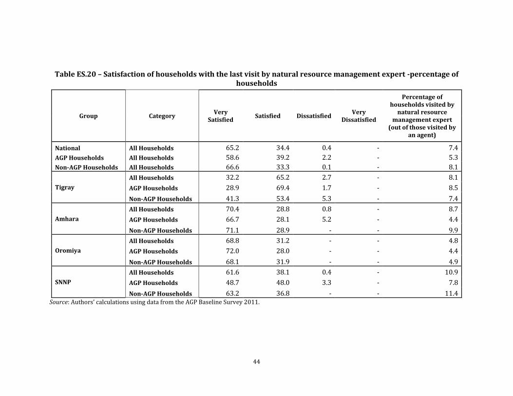
44
Table ES.20 – Satisfaction of households with the last visit by natural resource management expert -percentage of households
Group Category Very
Satisfied Satisfied Dissatisfied
Very Dissatisfied
Percentage of households visited by
natural resource management expert
(out of those visited by an agent)
National All Households 65.2 34.4 0.4 - 7.4
AGP Households All Households 58.6 39.2 2.2 - 5.3
Non-AGP Households All Households 66.6 33.3 0.1 - 8.1
Tigray
All Households 32.2 65.2 2.7 - 8.1
AGP Households 28.9 69.4 1.7 - 8.5
Non-AGP Households 41.3 53.4 5.3 - 7.4
Amhara
All Households 70.4 28.8 0.8 - 8.7
AGP Households 66.7 28.1 5.2 - 4.4
Non-AGP Households 71.1 28.9 - - 9.9
Oromiya
All Households 68.8 31.2 - - 4.8
AGP Households 72.0 28.0 - - 4.4
Non-AGP Households 68.1 31.9 - - 4.9
SNNP
All Households 61.6 38.1 0.4 - 10.9
AGP Households 48.7 48.0 3.3 - 7.8
Non-AGP Households 63.2 36.8 - - 11.4 Source: Authors’ calculations using data from the AGP Baseline Survey 2011.

45
Table ES.21 – Satisfaction of households with the last visit to FTCs -percentage of households
Group Category Very
Satisfied Satisfied Dissatisfied Very
Dissatisfied
Percentage of households who
visited FTC (Farmer training
Centers)
National All Households 63.4 35.9 0.6 0.2 5.7 AGP Households All Households 56.3 42.2 0.9 0.7 6.2 Non-AGP Households All Households 65.6 33.9 0.5 - 5.6
All Households 46.5 50.6 2.9 - 8.7
Tigray AGP Households 36.2 60.9 3.0 - 6.9 Non-AGP Households 60.5 36.8 2.8 - 11.9
All Households 55.1 44.7 - 0.2 4.5
Amhara AGP Households 60.3 38.4 - 1.3 4.1 Non-AGP Households 54.1 45.9 - - 4.6
All Households 83.0 16.7 - 0.3 4.7
Oromiya AGP Households 53.6 45.1 - 1.4 5.5 Non-AGP Households 93.0 7.0 - - 4.5
All Households 54.6 44.4 1.0 - 8.4
SNNP AGP Households 63.5 35.2 - 1.3 10.6 Non-AGP Households 52.1 47.0 0.9 - 8.0
Source: Authors’ calculations using data from the AGP Baseline Survey 2011.

46
Table ES.22. Yield in quintals for root crops, chat, enset, and coffee by AGP status and region
Group Category2 Statistic2 Root
Crops Chat Enset Coffee
National All HHHs
Mean 46.6 130.6 52.3 12.1
Median 24.0 4.7 10.0 3.4
SD 64.5 677.9 203.3 40.4
AGP woredas All HHHs
Mean 46.4 189.1 34.8 16.8
Median 20.0 640.0 10.0 3.6
SD 66.8 1029.6 119.1 49.2
Non-AGP woredas
All HHHs
Mean 46.6 108.2 57.9 11.0
Median 24.0 400.0 9.3 3.3
SD 63.9 477.9 223.2 37.9
Tigray
All Households
Mean 39.8 109.0 3.5 0.0
Median 12.1 9.0 0.5 0.0
SD 64.9 229.3 7.4 0.0
AGP Households
Mean 37.3 114.4 2.1 0.0
Median 12.0 9.0 0.5 0.0
SD 58.5 233.6 2.6 0.0
Non-AGP Households
Mean 42.8 0.0 5.2 0.0
Median 15.0 0.0 0.3 0.0
SD 71.8 0.0 10.5 0.0
Amhara
All Households
Mean 66.0 23.5 15.9 10.1
Median 32.0 2.5 3.2 1.5
SD 86.1 65.1 39.0 10.5
AGP Households
Mean 68.1 34.3 22.1 10.1
Median 34.1 2.5 3.2 1.5
SD 86.8 76.2 49.0 10.5
Non-AGP Households
Mean 65.3 0.1 6.5 0.0
Median 32.0 0.1 3.2 0.0
SD 85.9 0.0 7.5 0.0
Oromiya
All Households
Mean 47.6 173.0 10.4 55.2
Median 30.0 18.0 2.4 16.0
SD 62.1 641.2 40.0 120.9
AGP Households
Mean 51.3 36.5 11.3 47.7
Median 30.0 7.2 2.7 20.0
SD 66.6 201.7 33.6 126.5
Non-AGP Households
Mean 46.8 234.6 10.2 62.8
Median 30.0 24.0 2.4 16.0
SD 61.0 752.5 40.9 114.4
SNNP
All Households
Mean 29.1 107.3 13.2 51.9
Median 17.5 3.2 5.0 8.5
SD 37.9 706.0 40.8 213.0
AGP Households
Mean 21.1 317.2 18.6 30.0
Median 14.0 6.1 5.0 8.3
SD 28.0 1378.2 55.7 116.0
Non-AGP Households
Mean 31.4 40.3 11.9 57.4
Median 20.0 3.2 5.0 8.5
SD 40.0 181.1 35.9 230.7
Source: Authors’ calculations using data from the AGP Baseline Survey 2011.

47
Table ES.23. Extension service provided for root crops, chat, enset, and coffee on preparation of land by AGP status and region
Group Category Root Crops Chat Enset Coffee
National All Households 35.8 23.9 24.1 26.6
AGP woreda All Households 34.2 14.6 20.6 23.6
Non-AGP woreda All Households 36.2 27.5 25.2 27.3
Tigray
All Households 65.7 6.1 - 23.5
AGP Households 70.7 0.0 - 37.2
Non-AGP Households 58.0 64.8 - 0.0
Amhara
All Households 45.5 12.6 100.0 25.7
AGP Households 51.1 30.6 100.0 27.1
Non-AGP Households 44.1 0.0 - 23.9
Oromiya
All Households 28.2 19.5 13.4 23.8
AGP Households 26.3 7.5 16.3 15.4
Non-AGP Households 28.7 24.7 11.3 24.8
SNNP
All Households 39.5 27.4 26.6 29.7
AGP Households 30.3 20.1 22.8 27.5
Non-AGP Households 42.7 29.9 27.6 30.2
Source: Authors’ calculations using data from the AGP Baseline Survey 2011.
Table ES.24. Extension service provided for root crops, chat, enset, and coffee on seed planting methods by AGP status and region
Group Category Root Crops Chat Enset Coffee
National All Households 36.9 20.1 22.1 23.8
AGP woreda All Households 35.4 14.2 19.8 22.1
Non AGP woreda All Households 37.3 22.5 22.8 24.2
Tigray
All Households 68.9 6.1 - 18.4
AGP Households 76.1 0.0 - 29.2
Non-AGP Households 58.0 64.8 - 0.0
Amhara
All Households 44.8 9.7 100.0 24.5
AGP Households 51.1 23.5 100.0 25.0
Non-AGP Households 43.2 0.0 - 23.9
Oromiya
All Households 30.0 17.4 12.4 20.8
AGP Households 29.5 6.8 16.2 14.6
Non-AGP Households 30.1 22.0 9.5 21.5
SNNP
All Households 40.8 22.5 24.3 26.9
AGP Households 29.5 20.1 21.5 25.9
Non-AGP Households 44.9 23.2 25.1 27.2
Source: Authors’ calculations using data from the AGP Baseline Survey 2011.
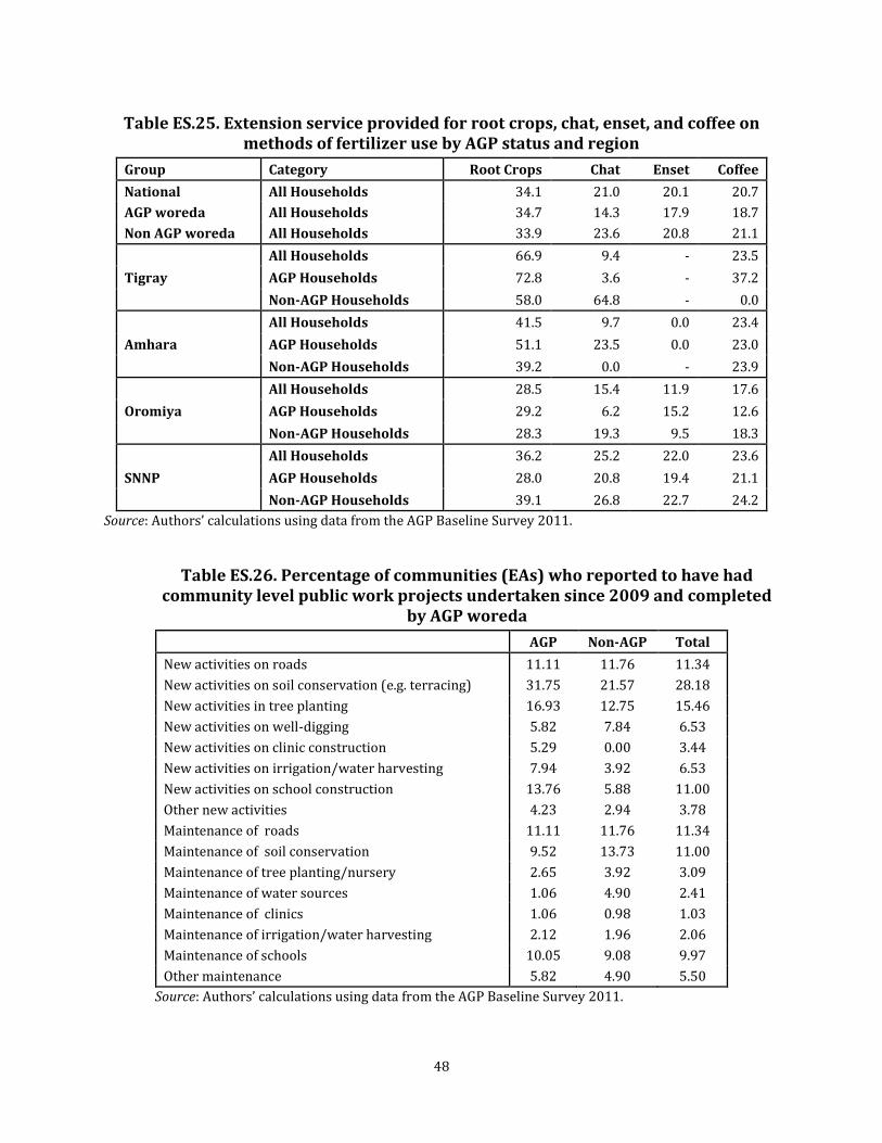
48
Table ES.25. Extension service provided for root crops, chat, enset, and coffee on methods of fertilizer use by AGP status and region
Group Category Root Crops Chat Enset Coffee
National All Households 34.1 21.0 20.1 20.7
AGP woreda All Households 34.7 14.3 17.9 18.7
Non AGP woreda All Households 33.9 23.6 20.8 21.1
Tigray
All Households 66.9 9.4 - 23.5
AGP Households 72.8 3.6 - 37.2
Non-AGP Households 58.0 64.8 - 0.0
Amhara
All Households 41.5 9.7 0.0 23.4
AGP Households 51.1 23.5 0.0 23.0
Non-AGP Households 39.2 0.0 - 23.9
Oromiya
All Households 28.5 15.4 11.9 17.6
AGP Households 29.2 6.2 15.2 12.6
Non-AGP Households 28.3 19.3 9.5 18.3
SNNP
All Households 36.2 25.2 22.0 23.6
AGP Households 28.0 20.8 19.4 21.1
Non-AGP Households 39.1 26.8 22.7 24.2
Source: Authors’ calculations using data from the AGP Baseline Survey 2011.
Table ES.26. Percentage of communities (EAs) who reported to have had community level public work projects undertaken since 2009 and completed
by AGP woreda
AGP Non-AGP Total
New activities on roads 11.11 11.76 11.34
New activities on soil conservation (e.g. terracing) 31.75 21.57 28.18
New activities in tree planting 16.93 12.75 15.46
New activities on well-digging 5.82 7.84 6.53
New activities on clinic construction 5.29 0.00 3.44
New activities on irrigation/water harvesting 7.94 3.92 6.53
New activities on school construction 13.76 5.88 11.00
Other new activities 4.23 2.94 3.78
Maintenance of roads 11.11 11.76 11.34
Maintenance of soil conservation 9.52 13.73 11.00
Maintenance of tree planting/nursery 2.65 3.92 3.09
Maintenance of water sources 1.06 4.90 2.41
Maintenance of clinics 1.06 0.98 1.03
Maintenance of irrigation/water harvesting 2.12 1.96 2.06
Maintenance of schools 10.05 9.08 9.97
Other maintenance 5.82 4.90 5.50
Source: Authors’ calculations using data from the AGP Baseline Survey 2011.
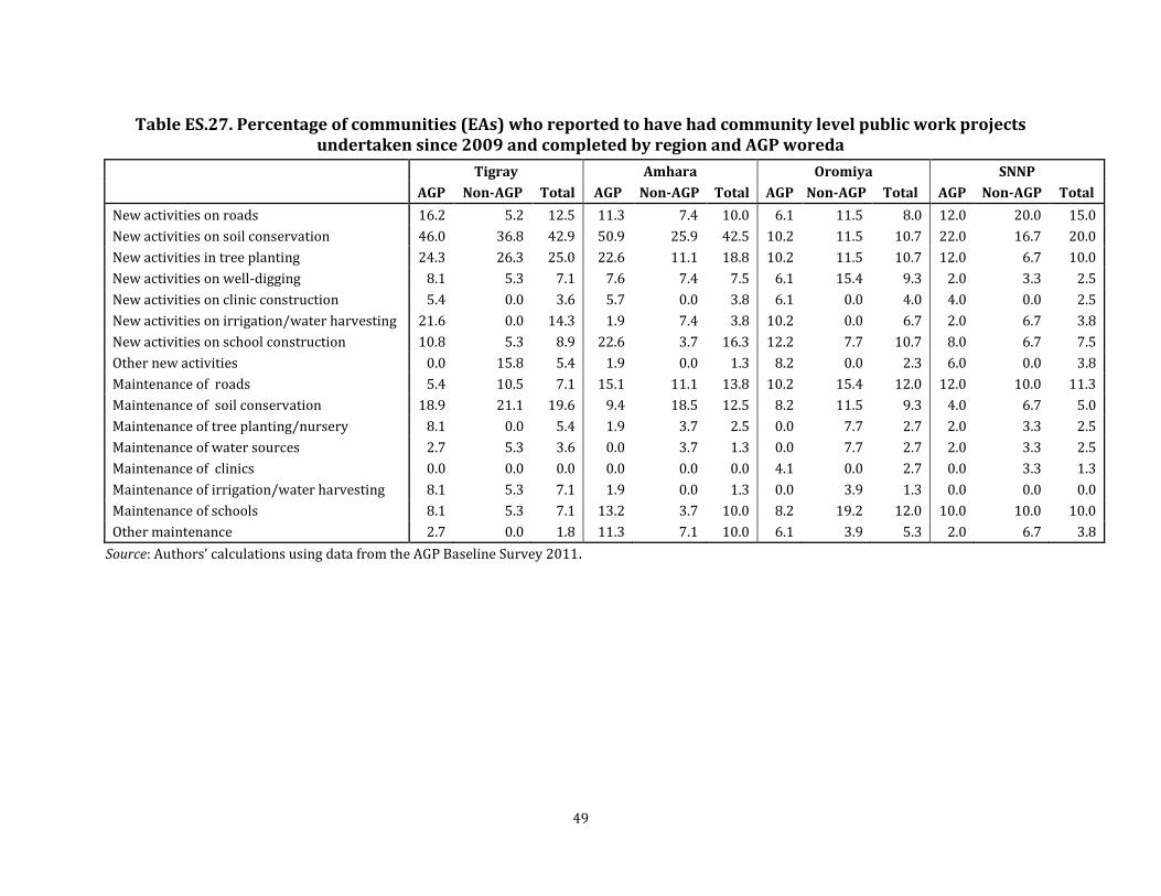
49
Table ES.27. Percentage of communities (EAs) who reported to have had community level public work projects undertaken since 2009 and completed by region and AGP woreda
Tigray Amhara Oromiya SNNP
AGP Non-AGP Total AGP Non-AGP Total AGP Non-AGP Total AGP Non-AGP Total
New activities on roads 16.2 5.2 12.5 11.3 7.4 10.0 6.1 11.5 8.0 12.0 20.0 15.0
New activities on soil conservation 46.0 36.8 42.9 50.9 25.9 42.5 10.2 11.5 10.7 22.0 16.7 20.0
New activities in tree planting 24.3 26.3 25.0 22.6 11.1 18.8 10.2 11.5 10.7 12.0 6.7 10.0
New activities on well-digging 8.1 5.3 7.1 7.6 7.4 7.5 6.1 15.4 9.3 2.0 3.3 2.5
New activities on clinic construction 5.4 0.0 3.6 5.7 0.0 3.8 6.1 0.0 4.0 4.0 0.0 2.5
New activities on irrigation/water harvesting 21.6 0.0 14.3 1.9 7.4 3.8 10.2 0.0 6.7 2.0 6.7 3.8
New activities on school construction 10.8 5.3 8.9 22.6 3.7 16.3 12.2 7.7 10.7 8.0 6.7 7.5
Other new activities 0.0 15.8 5.4 1.9 0.0 1.3 8.2 0.0 2.3 6.0 0.0 3.8
Maintenance of roads 5.4 10.5 7.1 15.1 11.1 13.8 10.2 15.4 12.0 12.0 10.0 11.3
Maintenance of soil conservation 18.9 21.1 19.6 9.4 18.5 12.5 8.2 11.5 9.3 4.0 6.7 5.0
Maintenance of tree planting/nursery 8.1 0.0 5.4 1.9 3.7 2.5 0.0 7.7 2.7 2.0 3.3 2.5
Maintenance of water sources 2.7 5.3 3.6 0.0 3.7 1.3 0.0 7.7 2.7 2.0 3.3 2.5
Maintenance of clinics 0.0 0.0 0.0 0.0 0.0 0.0 4.1 0.0 2.7 0.0 3.3 1.3
Maintenance of irrigation/water harvesting 8.1 5.3 7.1 1.9 0.0 1.3 0.0 3.9 1.3 0.0 0.0 0.0
Maintenance of schools 8.1 5.3 7.1 13.2 3.7 10.0 8.2 19.2 12.0 10.0 10.0 10.0
Other maintenance 2.7 0.0 1.8 11.3 7.1 10.0 6.1 3.9 5.3 2.0 6.7 3.8
Source: Authors’ calculations using data from the AGP Baseline Survey 2011.

50
Table ES.28. Average and proportion of revenue collected from the sale of livestock products by region and AGP status
Group Categories Variables Cattle Shoats Pack
Animals Chicken Total
National All Households Average revenue (in Birr) 1,037 177 64 64 1,344
Proportion (in %) 77 13 5 5 100
AGP Households
All Households Average revenue (in Birr) 801 155 49 30 1,044
Proportion (in %) 77 15 5 3 100
Non-AGP Households
All Households Average revenue (in Birr) 1,111 184 69 75 1,438
Proportion (in %) 77 13 5 5 100
Tigray
All Households Average revenue (in Birr) 688 205 23 31 1,001
Proportion (in %) 69 21 2 3 100
AGP Households Average revenue (in Birr) 728 218 19 27 1,079
Proportion (in %) 67 20 2 3 100
Non-AGP Households
Average revenue (in Birr) 621 184 29 36 871
Proportion (in %) 71 21 3 4 100
Amhara
All Households Average revenue (in Birr) 742 222 64 25 1,053
Proportion (in %) 70 21 6 2 100
AGP Households Average revenue (in Birr) 751 144 34 32 962
Proportion (in %) 78 15 4 3 100
Non-AGP Households
Average revenue (in Birr) 736 263 80 21 1,102
Proportion (in %) 67 24 7 2 100
Oromiya
All Households Average revenue (in Birr) 1,356 195 84 122 1,758
Proportion (in %) 77 11 5 7 100
AGP Households Average revenue (in Birr) 951 192 73 33 1,250
Proportion (in %) 76 15 6 3 100
Non-AGP Households
Average revenue (in Birr) 1,491 197 87 152 1,927
Proportion (in %) 77 10 5 8 100
SNNP
All Households Average revenue (in Birr) 834 89 32 7 963
Proportion (in %) 87 9 3 1 100
AGP Households Average revenue (in Birr) 479 83 12 8 587
Proportion (in %) 82 14 2 1 100
Non-AGP Households
Average revenue (in Birr) 953 91 39 7 1,089
Proportion (in %) 88 8 4 1 100
Source: Authors’ calculations using data from the AGP Baseline Survey 2011.

51
Table ES.29. Average and proportion of revenue collected from the sale of crops, by region and AGP status
Group Category Teff Barley Wheat Maize Sorghum Pulses Oil
seeds Vegeta
bles Root
Crops Fruit Crops
Chat Coffee Enset Total
National All Households 264.0 106.0 320.0 246.0 60.0 260.0 283.0 35.0 121.0 14.0 120.0 1309.0 11.0 3469.0 Proportion (%) 7.6 3.1 9.2 7.1 1.7 7.5 8.1 1.0 3.5 0.4 3.4 37.7 0.3 100.0
AGP woredas
All Households 427.0 132.0 404.0 249.0 107.0 284.0 881.0 113.0 137.0 17.0 420.0 1150.0 18.0 4637.0
Proportion (%) 9.2 2.8 8.7 5.4 2.3 6.1 19.0 2.4 3.0 0.4 9.1 24.8 0.4 100.0
Non-AGP woredas
All Households 214.0 98.0 294.0 245.0 45.0 252.0 98.0 11.0 116.0 14.0 27.0 1358.0 9.0 3109.0
Proportion (%) 6.9 3.2 9.5 7.9 1.5 8.1 3.2 0.4 3.7 0.4 0.9 43.7 0.3 100.0
Tigray
All Households 169.9 52.9 61.8 26.0 231.4 42.5 1369.8 17.5 173.6 0.3 6.4 3.0 0.0 2428.2
Proportion (in %) 7.0 2.2 2.5 1.1 9.5 1.8 56.4 0.7 7.1 0.0 0.3 0.1 0.0 100.0
AGP Households 139.7 51.3 58.8 32.9 336.9 53.2 2058.1 10.7 255.2 0.4 10.3 4.6 0.0 3212.8
Proportion (in %) 4.3 1.6 1.8 1.0 10.5 1.7 64.1 0.3 7.9 0.0 0.3 0.1 0.0 100.0
Non-AGP Households 218.3 55.5 66.5 14.9 62.4 25.4 266.1 28.3 42.6 0.0 0.0 0.5 0.0 1170.1
Proportion (in %) 18.7 4.7 5.7 1.3 5.3 2.2 22.7 2.4 3.6 0.0 0.0 0.0 0.0 100.0
Amhara
All Households 306.2 75.4 135.3 303.3 73.6 338.5 627.9 96.2 69.7 3.1 1.3 74.7 0.0 2807.8
Proportion (in %) 10.9 2.7 4.8 10.8 2.6 12.1 22.4 3.4 2.5 0.1 0.0 2.7 0.0 100.0
AGP Households 364.3 157.1 274.7 802.7 57.6 322.2 1726.8 256.1 86.4 8.5 2.6 176.1 0.0 6029.2
Proportion (in %) 6.0 2.6 4.6 13.3 1.0 5.3 28.6 4.2 1.4 0.1 0.0 2.9 0.0 100.0
Non-AGP Households 274.9 31.4 60.3 34.2 82.2 347.4 35.9 10.1 60.6 0.2 0.6 20.1 0.0 1072.1
Proportion (in %) 25.6 2.9 5.6 3.2 7.7 32.4 3.3 0.9 5.7 0.0 0.1 1.9 0.0 100.0
Oromiya
All Households 291.0 154.1 565.0 318.6 70.0 265.9 175.6 16.1 201.8 21.4 58.4 1480.8 2.8 3857.6
Proportion (in %) 7.5 4.0 14.6 8.3 1.8 6.9 4.6 0.4 5.2 0.6 1.5 38.4 0.1 100.0
AGP Households 627.4 206.6 684.0 161.1 112.9 432.8 181.8 13.8 200.2 23.0 158.5 703.6 11.7 3725.6
Proportion (in %) 16.8 5.5 18.4 4.3 3.0 11.6 4.9 0.4 5.4 0.6 4.3 18.9 0.3 100.0
Non-AGP Households 182.3 137.2 526.6 369.5 56.1 212.0 173.6 16.9 202.4 20.9 26.1 1731.9 0.0 3900.3
Proportion (in %) 4.7 3.5 13.5 9.5 1.4 5.4 4.4 0.4 5.2 0.5 0.7 44.4 0.0 100.0
SNNP
All Households 183.4 59.6 110.0 81.7 9.8 190.7 1.1 7.9 27.9 15.4 360.2 2415.5 39.5 3579.2
Proportion (in %) 5.1 1.7 3.1 2.3 0.3 5.3 0.0 0.2 0.8 0.4 10.1 67.5 1.1 100.0
AGP Households 71.2 76.1 61.9 153.4 28.0 125.9 4.2 10.8 26.2 12.2 1213.4 4272.7 54.9 6239.0
Proportion (in %) 1.1 1.2 1.0 2.5 0.4 2.0 0.1 0.2 0.4 0.2 19.4 68.5 0.9 100.0
Non-AGP Households 222.6 53.8 126.8 56.6 3.4 213.4 0.0 6.9 28.5 16.6 62.0 1766.5 34.1 2649.6
Proportion (in %) 8.4 2.0 4.8 2.1 0.1 8.1 0.0 0.3 1.1 0.6 2.3 66.7 1.3 100.0
Source: Authors’ calculations using data from the AGP Baseline Survey 2011.
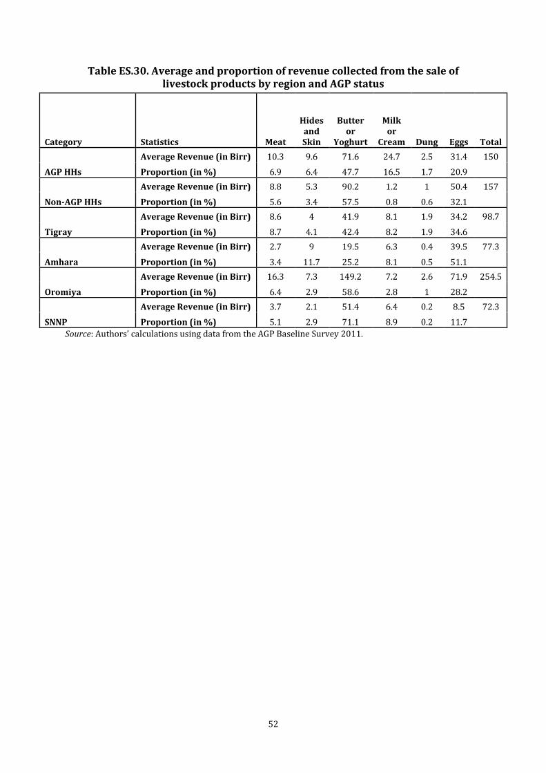
52
Table ES.30. Average and proportion of revenue collected from the sale of livestock products by region and AGP status
Category Statistics Meat
Hides and Skin
Butter or
Yoghurt
Milk or
Cream Dung Eggs Total
AGP HHs
Average Revenue (in Birr) 10.3 9.6 71.6 24.7 2.5 31.4 150
Proportion (in %) 6.9 6.4 47.7 16.5 1.7 20.9
Non-AGP HHs
Average Revenue (in Birr) 8.8 5.3 90.2 1.2 1 50.4 157
Proportion (in %) 5.6 3.4 57.5 0.8 0.6 32.1
Tigray
Average Revenue (in Birr) 8.6 4 41.9 8.1 1.9 34.2 98.7
Proportion (in %) 8.7 4.1 42.4 8.2 1.9 34.6
Amhara
Average Revenue (in Birr) 2.7 9 19.5 6.3 0.4 39.5 77.3
Proportion (in %) 3.4 11.7 25.2 8.1 0.5 51.1
Oromiya
Average Revenue (in Birr) 16.3 7.3 149.2 7.2 2.6 71.9 254.5
Proportion (in %) 6.4 2.9 58.6 2.8 1 28.2
SNNP
Average Revenue (in Birr) 3.7 2.1 51.4 6.4 0.2 8.5 72.3
Proportion (in %) 5.1 2.9 71.1 8.9 0.2 11.7
Source: Authors’ calculations using data from the AGP Baseline Survey 2011.

53
Chapter 1: The AGP Baseline Survey — Methodology and
Implementation
1.1. Background
Increased smallholder productivity and value-added in the agricultural sector are core elements
of the Ethiopian Government’s approach to poverty reduction. The Agricultural Growth Program
(AGP) is a component of this broad effort that will commence in 2011.3 The AGP, as proposed, is
a five-year program which has as the primary objective “to increase agricultural productivity
and market access for key crop and livestock products in targeted woredas with increased
participation of women and youth”. The AGP will:
Focus on agricultural productivity growth;
Target 83 woredas in Amhara, Oromiya, SNNP, and Tigray — woredas deemed to possess
high agricultural growth potential that can be realized with appropriate interventions (see
Figure 1.1 for a map and Annex Table A.1.1 for the list of AGP woredas)4;
Identify key commodities based on a variety of considerations — from current share in
production and potential marketability to possibilities for spatial spill-over effects; and
Emphasize greater participation of women and young people.
The AGP has two main components. Agricultural Production and Commercialization constitutes
the first component and its objectives are: “to strengthen the capacity of farmer organizations
and their service providers to scale up best practices and adopt improved technologies in
production and processing, and to strengthen marketing and processing of selected
commodities through engagement with private sector stakeholders”. The second component,
Small-scale Rural Infrastructure Development and Management, will “support the construction,
rehabilitation and/or improvement, and management of small-scale rural infrastructure to
improve productivity, and to further develop and increase the efficiency of key value chains
through improved access to markets.”
3 The details regarding the AGP are drawn from MoARD (June, 2010) and World Bank (September, 2010). 4 The number of woredas covered by the AGP has more recently been expanded to 96.
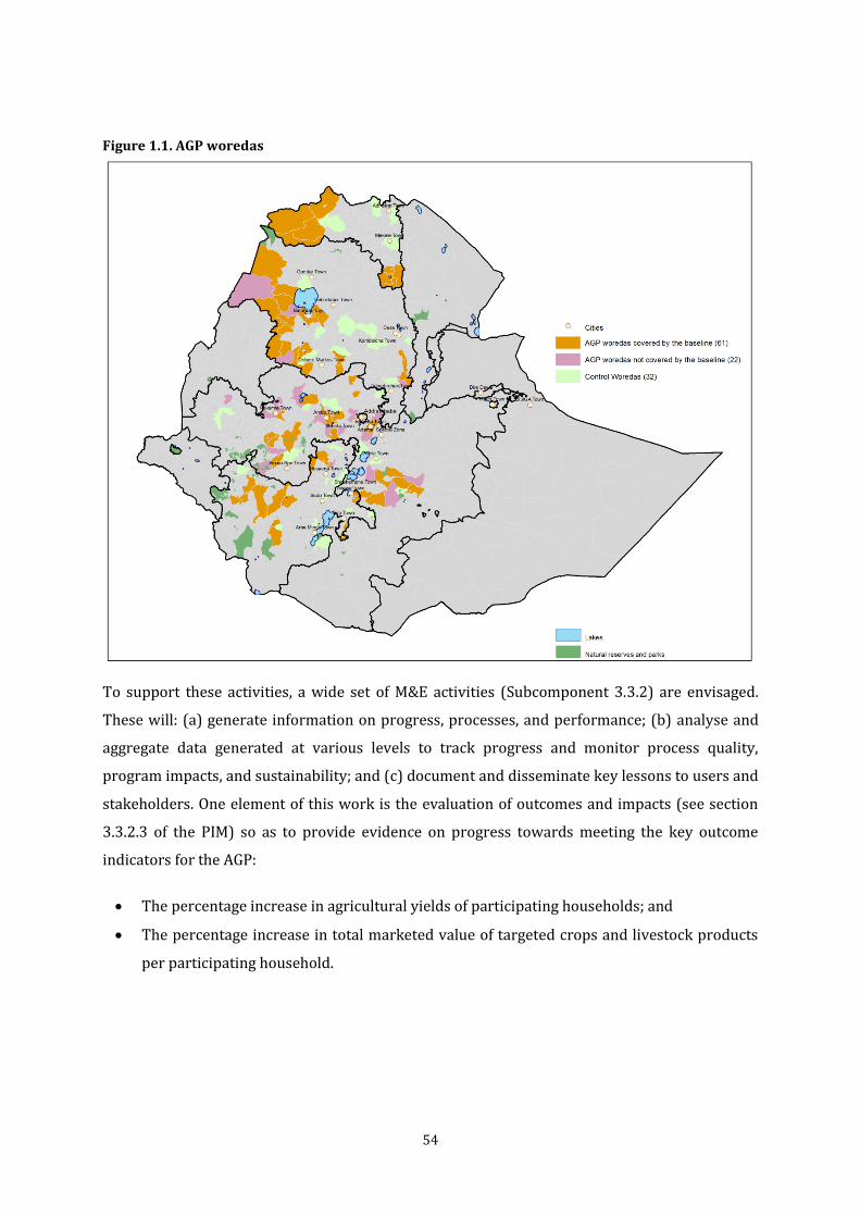
54
Figure 1.1. AGP woredas
To support these activities, a wide set of M&E activities (Subcomponent 3.3.2) are envisaged.
These will: (a) generate information on progress, processes, and performance; (b) analyse and
aggregate data generated at various levels to track progress and monitor process quality,
program impacts, and sustainability; and (c) document and disseminate key lessons to users and
stakeholders. One element of this work is the evaluation of outcomes and impacts (see section
3.3.2.3 of the PIM) so as to provide evidence on progress towards meeting the key outcome
indicators for the AGP:
The percentage increase in agricultural yields of participating households; and
The percentage increase in total marketed value of targeted crops and livestock products
per participating household.

55
1.2. Objectives of the Impact Evaluation of the AGP
IFPRI’s Ethiopia Strategy Support Program (ESSP) will support the AGP through the
development and implementation of an impact evaluation strategy.5 The discussion below
outlines the proposed evaluation strategy. We begin by outlining general issues associated with
any impact evaluation. We discuss specific features of the AGP that affect how it can be evaluated
and, based on these, propose a general approach for the impact evaluation of the AGP.
1.3. Methodology — Impact Evaluation
General Design Issues
The purpose of an impact evaluation is to compare outcomes for beneficiaries of a program to
what those outcomes would have been had they not received the program. The difference
between the observed outcomes for beneficiaries and these counterfactual outcomes represent
the causal impact of the program. The fundamental challenge of an impact evaluation is that it is
not possible to observe program beneficiaries in the absence of the program; the counterfactual
outcomes for beneficiaries are unknown. All evaluation strategies are designed to find a method
for constructing a proxy for these counterfactual outcomes. Most evaluations measure
counterfactual outcomes for beneficiaries by constructing a comparison group of similar
households from among non-beneficiaries. Collecting data on this comparison group makes it
possible to observe changes in outcomes without the program and to control for some other
factors that affect the outcome, which reduces bias in the impact estimates.
Figure 1.2 shows how information on a comparison group can be used to measure program
impact. In the figure, the outcome variable (say crop yields) is represented on the Y axis and
time is represented on the X axis. A household survey is conducted to measure yields in two
periods, the baseline at 0t and the follow-up at 1t . In the figure, at baseline the average outcome
for both the households benefiting from the intervention and those in the comparison group is at
the level of 0Y . After the program, at 1t , the intervention group has yields of level 1Y , while the
comparison group has an outcome level of
1Y . The impact of the program is measured
5 “The indicators in the Results Framework will ... [guide] the design [of] the baseline and impact evaluation questions and sampling as the programs outcomes will be measured against these indicators. In addition to the baseline two impact evaluations are planned: a mid-term impact evaluation in FY3 and a final impact evaluation in FY5. The baseline is planned before the project launch. The data collection for the baseline, mid-term impact evaluation and final impact evaluation will be conducted by the Central Statistical Agency (CSA). The Ethiopia Strategy Support Program Phase II will complement the work of CSA. In particular, ESSP would develop the survey instrument ... and the sampling process, as well as to analyze the data and write the impact evaluation reports.” (PIM, p. 96).

56
as 11 YY . If a comparison group had not been included, the impact might have been
misrepresented (and overstated) as the observed change in the outcome for the beneficiary
group, 01 YY .
In constructing a comparison group for the evaluation, it is important to ensure that the
comparison group is as similar as possible to the program beneficiaries before the start of the
program. To understand why, consider estimating the impact of the AGP on crop yields as the
difference in average crop yields between beneficiaries and a random sample of non-
beneficiaries. The problem with this approach is that non-beneficiaries are different from
program beneficiaries in ways that make them an ineffective comparison group. For example,
suppose that AGP participants have higher levels of schooling, greater knowledge of good
farming practices or are more entrepreneurial than non-participants, and they have
demonstrated their interest by participating in the program (this latter factor is sometimes
referred to as self-selection bias). If the evaluation does not control for these pre-program
differences, impact estimates will be biased. Put it another way, a simple comparison of AGP
participants and non-participants cannot distinguish between changes in crop yields brought
about by the AGP from those that result from the pre-existing differences in participants and
non-participants.
Figure 1.2. Measuring impact from outcomes from beneficiary and comparison groups
There are three ways by which a comparison group can be constructed: randomization,
regression discontinuity design (RDD), and matching. Randomization is widely considered to be
one of the most powerful approaches to construct a comparison group for an evaluation. The
method involves randomly assigning the program among comparably eligible communities or
57
households. Those that are randomly selected out of the program form a control group, while
those selected for the program are the treatment group. RDD is appropriate when there is a
strict cut-off applied that determines program eligibility. Individuals (or households) either side
of this cut-off are compared on the assumption that those ineligible (for example, households
just above a threshold value used as the cut-off) are virtually identical those that are eligible (for
example, households just below the threshold value used as the cut-off). Matching involves the
statistical construction of a comparison group of, say households that are sufficiently similar to
the treatment group before the program that they serve as a good indication of what the
counterfactual outcomes would have been for the treatment group. One popular approach is to
match program beneficiaries to a sub-sample of similar non-beneficiaries from the same or
neighbouring communities using a matching method such as propensity score matching (PSM),
nearest neighbour matching, or propensity weighted regression. Matching methods choose
communities or households as a comparison group based on their similarity in observable
variables correlated with the probability of being in the program and with the outcome. All
matching methods measure program impact as the difference between average outcomes for
treated households and a weighted average of outcomes for non-beneficiary households where
the weights are a function of observed variables.6
Aspects of the AGP Relevant to the Design of an Impact Evaluation Strategy
There are five aspects of the AGP that have a direct bearing on our choice of impact evaluation
strategy: purposive woreda selection; the demand driven nature of the AGP; household self-
selection into AGP activities; the presence of multiple interventions; and spill-over effects. We
discuss these, and their implications for evaluation, in turn.
Purposive Woreda Selection: Woredas eligible for the AGP are those where existing location
factors are conducive for agricultural growth. Further, clustering of AGP woredas will assist the
program in making significant impact within the targeted areas. The criteria for selection of AGP
woredas include:
Access to markets (access to cities of 50,000 population or over in less than 5 hours);
Natural resource endowments;
Suitable rainfall and soil for crop and fodder production;
Potential for development of small-scale irrigation facilities;
6 The difference between alternative matching methods centres on various methods for constructing the weights for measuring impact.

58
Institutional plurality of service providers, including good basis and growth of viable
cooperatives and farmer groups; and existing partnership engagements with private
sector; and
Willingness and commitment to participate.
Purposive woreda selection means that an evaluation design based on randomizing access to the
AGP at the woreda level is infeasible. It also implies that an RDD design at the woreda or even
the enumeration area (EA) level is infeasible given that there is not a single, strict metric that
determines eligibility.
Demand Driven AGP and Household Self Selection: The AGP is intended to be demand-driven.
Households will choose what activities they will undertake and the extent of their participation.
As stated in the PIM:
Bottom-up planning process will be practiced to give greater power to kebele- and
woreda-level development initiatives with particular attention to ensuring equal
and active participation of both women and men. Individual activities would be
largely chosen by farmers, communities and organizations as well as business
private sector at a grassroots level. Thus, local male and female farmers, youth,
women and private business enterprises are the owners of the program, and will
actively participate in problem identification, planning, implementation and
monitoring and evaluation of the activities. (PIM, p. 9)
The demand driven, self-selected nature of the AGP means that at the household level, both
randomized and RDD designs are infeasible. Further, particular attention must be paid in
identifying those locality, household, and individual characteristics that affect the decision to
participate in an AGP activity.
Multiple Interventions: Participants in the AGP may benefit from a single intervention, from
multiple interventions, and from interventions with differing degrees of intensity. This needs to
be taken into account in the evaluation design and implementation.
Spill-over Effects: The AGP will benefit both program participants and non-participants. For
example, even if a household chooses not to actively participate in any AGP activities, it may
benefit from AGP activities such as the upgrading or construction of new feeder roads or
improved market centres. Consider a woreda where, as part of the AGP, an improved feeder road
is constructed and a package of improved seeds, fertilizers, and technical advice is provided to
households who have formed farmers groups. Comparing changes in outcome indicators

59
between households in these farmers groups and those households who are not members, will
underestimate the impact of the AGP for several reasons: all households, not just those in the
farmers groups, may benefit from the construction of feeder roads; knowledge gained by
members of farmers groups may be shared with non-members; and producer prices may rise if
higher output increases the number of traders buying in this locality.
The Impact Evaluation Strategy
The following impact evaluation strategy is proposed:
We will use double difference and matching methods to assess impact employing (as envisaged
in the PIM) a baseline survey fielded before the start of the AGP and follow-up surveys (also
envisaged in the PIM) to track both program implementation and estimate impact over time. We
propose these for three reasons: (a) they can be used to assess the impact of single or multiple
interventions; (b) they can estimate the impact of intensity of participation, not just whether a
household participates; and (c) other methods, such as randomization and RDD, are infeasible.
More specifically, matching estimates are improved by measuring outcomes for treatment and
comparison groups before and after the program begins. This makes it possible to construct
“difference-in-differences” (DID) estimates of program impact, defined as the average change in
the outcome in the treatment group, T, minus the average change in the outcome in the
comparison group, C. Mathematically, this is expressed as,
CCTTATT
DID yyyy 0101 .
The main strength of DID estimates of program impact is that they remove the effect of any
unobserved variables that represent persistent (time-invariant) differences between the
treatment and comparison group. This helps to control for the fixed component of various
contextual differences between treatment and comparison groups, including depth of markets,
agro-climatic conditions, and any persistent differences in infrastructure development. As a
result, DID estimates can lead to a substantial reduction in selection bias of estimated program
impact. As envisaged in existing AGP documentation, DID estimates will be feasible given the
intention to field baseline and two follow-up surveys.
We will pay careful attention to characteristics that affect selection and intensity of
participation. This provides useful programmatic information (What are the characteristics of
those who take part and those who do not? What does this imply in terms of program outreach

60
and the distribution of benefits within participating woredas?). It is also necessary for the
implementation of matching methods.
At the household and EA level (kebele level, to be precise), we will collect “bottom-up” data on
program implementation. This provides useful programmatic information as well as informing
our definition of “participation” in the AGP. We will also ensure that the baseline and follow-up
surveys are implemented in both AGP and non-AGP woredas so as to collect information that
allows us to examine spill-over effects.
1.4. Methodology — Sample Design
The first step in implementing this evaluation strategy is the collection and analysis of baseline
data. The nature and number of indicators to track as well as the coverage and level of
disaggregation have to be decided
Disaggregation
A key element of the evaluation design concerns the level or levels of disaggregation at which
AGP’s impact will be assessed. The AGP-PIM and AGP-PAD contain broad expressions of
preference regarding this issue. According to these documents, the two PDO indicators noted
above are to be further qualified with the following:
The indicators “will be monitored for the average household as well as separately for
female- and youth-headed households” (World Bank (September, 2010), p. 46).
“The impact evaluation study will disaggregate the indicators for the key agricultural
commodities by region.” (World Bank (September, 2010), p. 46)
“An impact evaluation will be conducted that will assess the increase achieved by the end
of implementation relative to the baseline in the area selected for intervention and relative
to areas without the intervention.” (World Bank (September, 2010), p. 8)
Thus, for example, a literal interpretation suggests that crop- and region-specific indicators are
to be monitored for classes of household-types (by gender and age of household heads) in
program and non-program woredas. Although appealing at face value, such an evaluation will
demand, among others, a rather large sample and an extensive data collection effort. It is thus
necessary to consider the extent of spatial and socio-economic disaggregation involved in the
impact assessment in light of survey and sampling requirements it entails.
61
As always, the design of the baseline survey reflects a compromise between coverage and cost.
To assist the AGP-TC in making a decision, the IFPRI team highlighted the challenges of
conducting a baseline and, subsequently, impact surveys to exhaustively and rigorously track
the indictors listed in the AGP-PIM and AGP-PAD. It also presented alternative scenarios
matching coverage and levels of disaggregation with cost. The AGP-TC decided to have a yield-
focused region-disaggregated baseline.
Sample Size Calculations
The first task in sample design is estimating the sample size needed for the baseline survey. In
brief, this involves the following: determine the appropriate level of statistical significance (the
sample has to be sufficiently large to minimize the chance of detecting an effect that does not
exist), and statistical power (the sample has to be sufficiently large to minimize the chance of not
detecting an effect that does exist). Additional determinants of sample size are variability of
project outcome indicators; the size of the design effect; the extent of program take up; assumed
response and attrition rates; and minimum detectable effect size.
The survey team, based on the decision of the AGP-TC noted above and in consultation with the
CSA, has determined sample size on the basis of the following:
Yield (primarily crop yield) measured from survey data is the primary outcome indicator;
The desired minimum detectable size effect is equivalent to 20 percent of (or 0.2)
standard deviation crop yield growth greater than that achieved in comparable but non-
AGP woredas;7
The target level of significance is 5% (two-tailed) and that of power is 80%;
Ninety percent of the households asked will agree to an interview (or the response rate is
90%);
The average uptake rate of 75% — i.e., on average, 75% of households who are offered
benefits via AGP will accept the offer. This leads to a variance in take-up rates of 0.1875;
The sample is divided in to two-third treated (or AGP woredas) and one-third control (or
non-AGP woredas);
The woreda being the cluster being targeted, it is proposed to sample 78 households per
woreda, with 26 households per enumeration area (EA)
7 Calculations using CSA’s Ethiopian Agricultural Sample Survey data for 2009/10 show that the standard deviation of
cereal yields is around 8.8 quintals such that a yield increase equivalent to 30 percent this is the same as a 15 percent growth in mean yield over the project period. Note that between 2007/08 and 2009/10 cereal yields grew at an average annual growth of 4 percent, which, if maintained for five years, will produce a total yield growth of 22 percent.
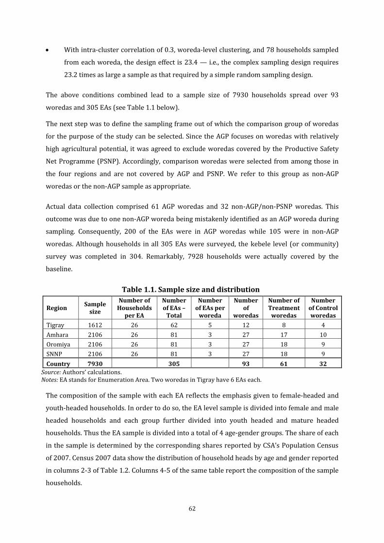
62
With intra-cluster correlation of 0.3, woreda-level clustering, and 78 households sampled
from each woreda, the design effect is 23.4 — i.e., the complex sampling design requires
23.2 times as large a sample as that required by a simple random sampling design.
The above conditions combined lead to a sample size of 7930 households spread over 93
woredas and 305 EAs (see Table 1.1 below).
The next step was to define the sampling frame out of which the comparison group of woredas
for the purpose of the study can be selected. Since the AGP focuses on woredas with relatively
high agricultural potential, it was agreed to exclude woredas covered by the Productive Safety
Net Programme (PSNP). Accordingly, comparison woredas were selected from among those in
the four regions and are not covered by AGP and PSNP. We refer to this group as non-AGP
woredas or the non-AGP sample as appropriate.
Actual data collection comprised 61 AGP woredas and 32 non-AGP/non-PSNP woredas. This
outcome was due to one non-AGP woreda being mistakenly identified as an AGP woreda during
sampling. Consequently, 200 of the EAs were in AGP woredas while 105 were in non-AGP
woredas. Although households in all 305 EAs were surveyed, the kebele level (or community)
survey was completed in 304. Remarkably, 7928 households were actually covered by the
baseline.
Table 1.1. Sample size and distribution
Region Sample
size
Number of Households
per EA
Number of EAs –
Total
Number of EAs per
woreda
Number of
woredas
Number of Treatment
woredas
Number of Control woredas
Tigray 1612 26 62 5 12 8 4
Amhara 2106 26 81 3 27 17 10
Oromiya 2106 26 81 3 27 18 9
SNNP 2106 26 81 3 27 18 9
Country 7930
305
93 61 32
Source: Authors’ calculations. Notes: EA stands for Enumeration Area. Two woredas in Tigray have 6 EAs each.
The composition of the sample with each EA reflects the emphasis given to female-headed and
youth-headed households. In order to do so, the EA level sample is divided into female and male
headed households and each group further divided into youth headed and mature headed
households. Thus the EA sample is divided into a total of 4 age-gender groups. The share of each
in the sample is determined by the corresponding shares reported by CSA’s Population Census
of 2007. Census 2007 data show the distribution of household heads by age and gender reported
in columns 2-3 of Table 1.2. Columns 4-5 of the same table report the composition of the sample
households.

63
Table 1.2. Household composition of EA sample
Share in the population of rural household heads – Census 2007 (%)
Share in the AGP baseline sample of
rural household heads – Census 2007 (%)
Implied post-stratification
weights
Male Female Male Female Male Female
Young (15-34 years of age) 29.6 (8) 5.4 (1) 30.8 (8) 7.7 (2) 0.961 0.701
Mature (35 years of age or older) 48.9 (12) 16.1 (5) 38.5 (10) 23.1 (6) 1.270 0.697
Source: Authors’ calculation using CSA data. Note: The numbers in brackets are implied (columns 2-3) and actual (columns 4-5) number of sample households in an EA (with the total being a predetermined 26).
Thus the AGP baseline slightly oversamples households headed by both young and mature
females relative to their share implied by Census 2007. In contrast, mature male headed
households are slightly under-sampled. In this regard, the baseline adopted the 15-34 years of
age as the relevant bracket in identifying young household heads. Note that the official definition
of youth in Ethiopia is from 13 to 34 years of age. However, Census 2007 does not report any
heads younger than 15 — thus the cut-off for the baseline.

64
Methodology — Household and Community Questionnaires
Two questionnaires were administered during the AGP baseline. Both were specifically designed
for the baseline in consultation with CSA and relevant stakeholders. The structure of these
questionnaires is outlined below:
Household questionnaire
Module Content 0 General information about the household location; tracking information for follow-
up surveys 1 Basic household characteristics 2 Land characteristics and use Crop production Input use in crop production 3 Crop output utilization and marketing 4 Agricultural extension, technology, and information networks 5 Livestock assets, production, and use 6 Household assets 7 Income apart from own agricultural activities and credit 8 Consumption: Non-food expenditures, food consumption, food availability, access,
and coping strategies 9 Shocks and poverty perceptions
Community questionnaire
Module Content
0 Site identification 1 Location and access
2 Household assets
3 Services (general)
4 Production and marketing
5 Technology adoption
6 Migration
7 Local wages
8 Food prices in the last year
9 Current food prices
The design of the questionnaires was guided by the AGP’s program objectives and indicators
thereof. Table 1.3 reports on this link.

65
Table 1.3. AGP program indictors and questionnaire sections
Development objective PDO indicators Questionnaire
module/section
Agricultural productivity and market access increased for key crop and livestock products in targeted woredas, with increased participation of women and youth.
Percentage increase in agricultural yield of participating households (index for basket crops and livestock products).
Module 2: Section 2
Module 5: Sections 1-2
Percentage increase in total real value of marketed agricultural (including livestock) products per participating household.
Module 3: Section 2
Module 5: Section 3
Sub-component 1.1: Institutional strengthening and development
Farmers have improved access to and quality of services through support from key public institutions and private organizations (groups).
Percentage of farmers satisfied with quality of extension services provided (disaggregated by service providers, type of service/technology, crop, and livestock).
Share of households that are members of functioning farmer organizations (disaggregated by group type).
Module 4
Sub-component 1.2: Scaling up best practices
Sub-projects for improved productivity, value addition, and marketing realized and sustainably managed.
Number of farm households with innovative best practices (improved/new techniques and technologies).
Number of sub-projects fully operational and sustainably managed 2 years after initial investments (disaggregated by type of investments).
Module 4
Sub-component 1.3: Market and agribusiness development
Key selected value chains strengthened.
Percentage real sales value increase of the key selected value chains commodities supported at the end of the value chain.
Community questionnaire:
Section 8
Sub-component 2.1: Small-scale agricultural water development and management.
Demand-driven infrastructure investments for improved agricultural productivity realized and sustainably managed.
Number of farmers benefiting from the irrigation investments (disaggregated by type of investments).
Percentage increase in area under irrigation.
Percentage increase in areas treated under sustainable land management.
Module 2 : Section 7
Sub-component 2.2: Small-scale market infrastructure development and management
Demand-driven infrastructure investments for improved access to market realized and sustainably managed.
Percentage decrease in time for farmers to travel to market centre.
Percentage of users satisfied with the quality of market centres.
Community questionnaire
Source: MoARD (June, 2010)
66
1.5. Data Collection
In line with the PIM, the CSA conducted the preparation and implementation of the household
and community surveys and the entry of data once collection was completed. IFPRI provided
support to CSA as it conducted these activities. Specifically, IFPRI staff: (a) assisted in the
training of CSA staff; (b) jointly developed enumerator manuals; (c) assisted with EA and
household selection; (d) provided technical support during survey implementation; (e) gave
technical advice in the development of the data entry programs. The same approach that IFPRI
and CSA have used in the fielding of household and community surveys for the evaluation of the
Productive Safety Net Programme was followed. Throughout all aspects of survey
implementation, managerial authority rested with CSA. IFPRI’s role is to provide technical
support and capacity building.
During May-June, 2011, the CSA, in collaboration with IFPRI, completed the design and
implementation of the survey methodology (including sampling strategy and sample selection),
preparation of questionnaires and manuals, selection and training of survey enumerators, and
delineation of EA and household listing. The actual data collection occurred during July 3-22,
2011.
Although data collection was completed as planned, date entry took much longer than initially
anticipated. The CSA planned to provide cleaned and processed raw data to MoA by November
13, 2011. Unfortunately, the second half of 2011 and the first couple of months of 2012 turned
out to be a very busy time for CSA with a number of periodic large surveys (HICE, DHS)
happening in addition to its annual ones during the period. As a consequence, the entry and
first-stage cleaning of the AGP baseline data could only be completed in March 2012. This led to
a considerable pressure to produce the baseline report in the time frame initially planned.
A Note on Sample Weights
Three steps were involved in the selection of households for the AGP baseline. First, the 61
woredas were randomly selected from among the 83 AGP woredas. Similarly, 32 woredas were
randomly selected from among non-PSNP and non-AGP woredas in the four regions within
which AGP operates (Amhara, Oromiya, SNNP, and Tigray). At the second stage, 3 EAs where
randomly chosen from among EAs in each woreda. Tigray is the exception to this rule because,
though the same number of households is demanded by the desired level of precision and
power, there are fewer woredas to include. Thus, 5 EAs each from ten woredas and 6 EAs each
from two woredas were selected in Tigray. The final step is the selection of 26 households from
within each EA. This is done based on a fresh listing of households residing within each EA and

67
selecting households randomly until the desired number and composition of households is
obtained.
Each household included in the AGP baseline sample represents a certain number of households
reflecting the selection probability associated with it. This number is its sample weight. All
descriptive statistics in this report are weighted by these sample weights.
68
Chapter 2: Characteristics of Households
This chapter adds to the last section of Chapter 1 in which we provided general features of the
study woredas. This section describes households in the study area in terms of their members’
(including heads) age, marital status, and occupation. Households are also described in terms of
physical assets and livestock they own as well as the type of houses they reside in.
2.1. Demographic Characteristics
As noted above, the design of the AGP baseline survey allows the generation of statistics that are
representative of not only the AGP woredas but also the non-PSNP rural woredas of the four
regions. According to this survey, an estimated 9.4 million rural households resided in these
woredas during 2011. In terms of coverage by AGP, of the total, 22.9 percent resided in woredas
planned to benefit from the AGP while the remaining 77.1 reside in non-AGP, non-PSNP
woredas. This chapter provides an overview of the demographic structure of these households.
The average age of a household head is 43 years with standard deviation of 15.6 years and a
median of 40 years. The age of the household head extends from 15 to 98 years old. When
disaggregated by gender, male headed households are younger at 41 years relative to females at
47.5 years (Table 2.1). The median age is relatively lower for male headed households, 36 years,
relative to female headed households, 46 years. The gap in the median age between male and
female headed households is even higher. As one would expect, households with mature headed
households have a higher mean, 51.9 years, than that of younger heads, only 28 years. Regarding
AGP status, on average household heads in non-AGP woredas are 0.2 years older than those in
AGP woredas which is almost equal in both woreda categories. The remaining statistics for
categories by AGP status also have a similar pattern as the national estimates.
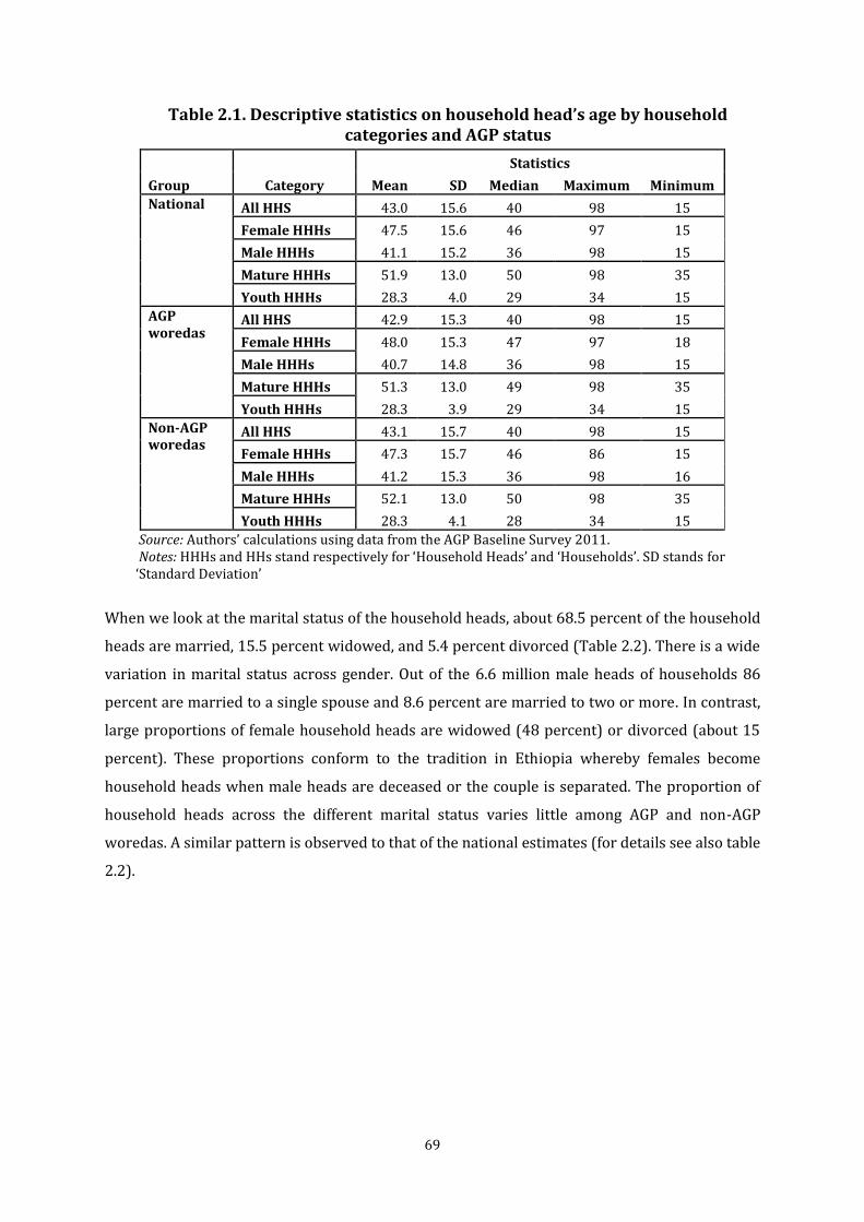
69
Table 2.1. Descriptive statistics on household head’s age by household categories and AGP status
Group Category
Statistics
Mean SD Median Maximum Minimum
National All HHS 43.0 15.6 40 98 15
Female HHHs 47.5 15.6 46 97 15
Male HHHs 41.1 15.2 36 98 15
Mature HHHs 51.9 13.0 50 98 35
Youth HHHs 28.3 4.0 29 34 15
AGP woredas
All HHS 42.9 15.3 40 98 15
Female HHHs 48.0 15.3 47 97 18
Male HHHs 40.7 14.8 36 98 15
Mature HHHs 51.3 13.0 49 98 35
Youth HHHs 28.3 3.9 29 34 15
Non-AGP woredas
All HHS 43.1 15.7 40 98 15
Female HHHs 47.3 15.7 46 86 15
Male HHHs 41.2 15.3 36 98 16
Mature HHHs 52.1 13.0 50 98 35
Youth HHHs 28.3 4.1 28 34 15
Source: Authors’ calculations using data from the AGP Baseline Survey 2011. Notes: HHHs and HHs stand respectively for ‘Household Heads’ and ‘Households’. SD stands for ‘Standard Deviation’
When we look at the marital status of the household heads, about 68.5 percent of the household
heads are married, 15.5 percent widowed, and 5.4 percent divorced (Table 2.2). There is a wide
variation in marital status across gender. Out of the 6.6 million male heads of households 86
percent are married to a single spouse and 8.6 percent are married to two or more. In contrast,
large proportions of female household heads are widowed (48 percent) or divorced (about 15
percent). These proportions conform to the tradition in Ethiopia whereby females become
household heads when male heads are deceased or the couple is separated. The proportion of
household heads across the different marital status varies little among AGP and non-AGP
woredas. A similar pattern is observed to that of the national estimates (for details see also table
2.2).

70
Table 2.2. Proportion of household head marital status by household categories and AGP status
Group Category Married,
single spouse
Single Divorced Widowed Separated
Married, more
than one spouse
National
All HHS 68.5 2.4 5.4 15.5 1.5 6.7
Female HHHs 28.6 2.2 14.7 48.3 4.0 2.2
Male HHHs 85.8 2.4 1.4 1.4 0.4 8.6
Mature HHHs 60.3 0.4 6.1 22.7 1.3 9.2
Youth HHHs 82.4 5.6 4.3 3.5 1.7 2.5
AGP woredas
All HHS 67.2 2.2 6.7 16.4 1.2 6.4
Female HHHs 24.2 1.4 18.3 50.7 3.2 2.2
Male HHHs 85.9 2.5 1.7 1.4 0.3 8.2
Mature HHHs 59.5 0.5 7.2 23.6 1.3 8.0
Youth HHHs 80.6 5.2 5.8 3.8 1.1 3.5
Non-AGP woredas
All HHS 69.0 2.4 5.0 15.3 1.5 6.8
Female HHHs 30.1 2.4 13.5 47.5 4.2 2.2
Male HHHs 85.7 2.4 1.3 1.4 0.4 8.8
Mature HHHs 60.5 0.4 5.7 22.4 1.3 9.5
Youth HHHs 82.9 5.7 3.8 3.5 1.9 2.3
Source: Authors’ calculations using data from the AGP Baseline Survey 2011. Notes: HHHs and HHs stand respectively for ‘Household Heads’ and ‘Households’.
With regards to the distribution of household size, there were 45.5 million household members
in the 9.4 million households surveyed, which is an average household size of about 4.9 persons
(Table 2.3). About 34 percent of the households have 3-4 members followed by 30 percent of
the households with 5-6 members (Figure 2.1). With 5.3 members, male headed households are
significantly larger than those with female heads that average 3.7 persons. The fact that 63
percent of female household heads are either widowed or divorced relative to the 95 percent
male heads who are married may partly explain this difference. The largest 2 categories of 3-4
and 5-6 members account for about 64 percent of the male headed households while
households with 1-2 and 3-4 members account for 71 percent of female headed households.

71
Figure 2.1. Distribution of household size
Source: Authors’ calculations using AGP baseline survey data.
As can be expected households with relatively younger heads have smaller sizes, averaging 4.3
members relative to the 5.2 members in the households with mature heads. Households with 3-
4 and 5-6 members dominate the youth categories at 76 percent, as well as the mature
categories at 57 percent. Although the difference is little, non-AGP woredas have larger
household sizes averaging 4.9 members relative to the 4.7 in AGP woredas. The difference is
also statistically significant. The distribution of household sizes is similar across AGP and non-
AGP woredas. However, there are differences in the proportions across mature and youth
headed households.
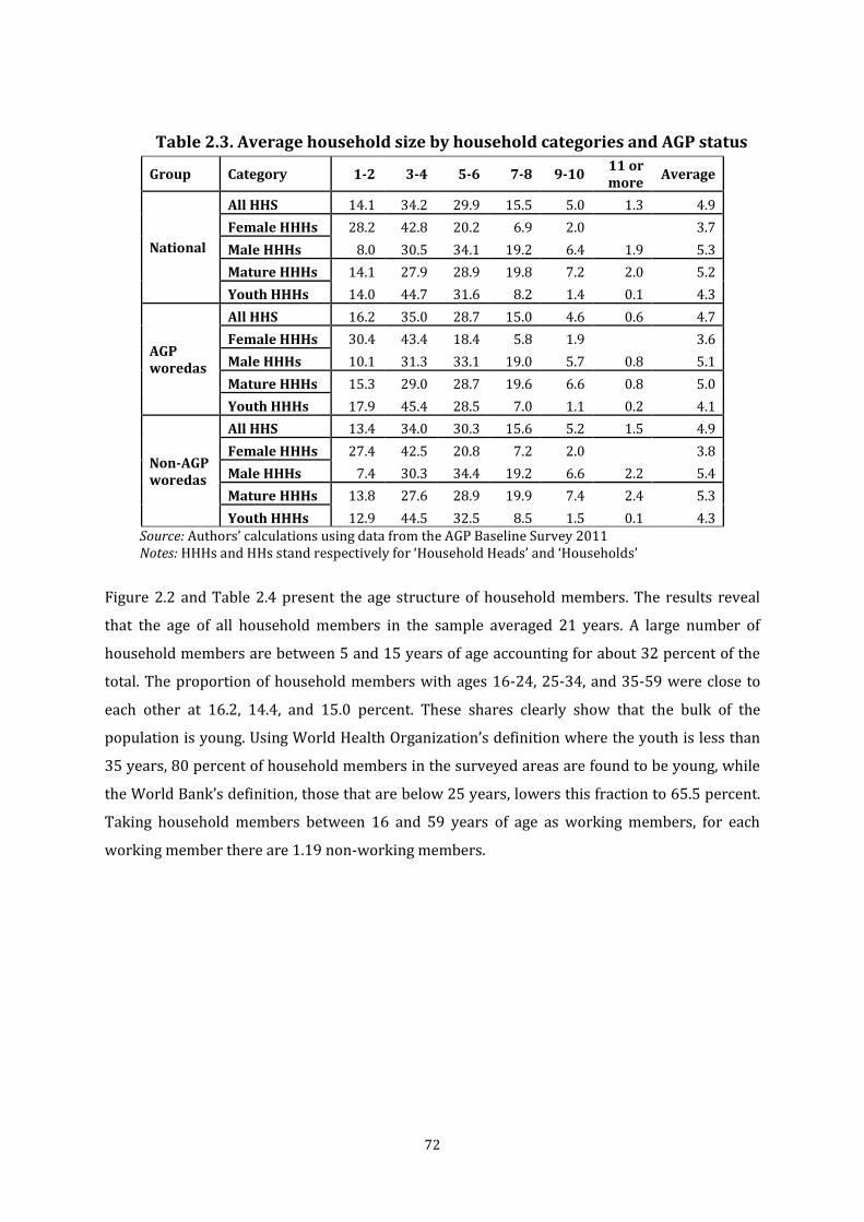
72
Table 2.3. Average household size by household categories and AGP status
Group Category 1-2 3-4 5-6 7-8 9-10 11 or more
Average
National
All HHS 14.1 34.2 29.9 15.5 5.0 1.3 4.9
Female HHHs 28.2 42.8 20.2 6.9 2.0 3.7
Male HHHs 8.0 30.5 34.1 19.2 6.4 1.9 5.3
Mature HHHs 14.1 27.9 28.9 19.8 7.2 2.0 5.2
Youth HHHs 14.0 44.7 31.6 8.2 1.4 0.1 4.3
AGP woredas
All HHS 16.2 35.0 28.7 15.0 4.6 0.6 4.7
Female HHHs 30.4 43.4 18.4 5.8 1.9 3.6
Male HHHs 10.1 31.3 33.1 19.0 5.7 0.8 5.1
Mature HHHs 15.3 29.0 28.7 19.6 6.6 0.8 5.0
Youth HHHs 17.9 45.4 28.5 7.0 1.1 0.2 4.1
Non-AGP woredas
All HHS 13.4 34.0 30.3 15.6 5.2 1.5 4.9
Female HHHs 27.4 42.5 20.8 7.2 2.0 3.8
Male HHHs 7.4 30.3 34.4 19.2 6.6 2.2 5.4
Mature HHHs 13.8 27.6 28.9 19.9 7.4 2.4 5.3
Youth HHHs 12.9 44.5 32.5 8.5 1.5 0.1 4.3 Source: Authors’ calculations using data from the AGP Baseline Survey 2011 Notes: HHHs and HHs stand respectively for ‘Household Heads’ and ‘Households’
Figure 2.2 and Table 2.4 present the age structure of household members. The results reveal
that the age of all household members in the sample averaged 21 years. A large number of
household members are between 5 and 15 years of age accounting for about 32 percent of the
total. The proportion of household members with ages 16-24, 25-34, and 35-59 were close to
each other at 16.2, 14.4, and 15.0 percent. These shares clearly show that the bulk of the
population is young. Using World Health Organization’s definition where the youth is less than
35 years, 80 percent of household members in the surveyed areas are found to be young, while
the World Bank’s definition, those that are below 25 years, lowers this fraction to 65.5 percent.
Taking household members between 16 and 59 years of age as working members, for each
working member there are 1.19 non-working members.

73
Figure 2.2. Age Structure of household members
Source: Authors’ calculations using AGP baseline survey data.
Excluding the 16-24 year old age group in which the proportion in female and male headed
households is about the same, in female headed households children under 15 accounted for
47.2 percent of all members while the corresponding number in male headed households was
about 49.8 percent. Considering all members, households with male heads have members about
2.5 years younger while considering members 5 years of age or older the difference drops to 1.4
years.
Members in non-AGP households were relatively older and this holds across genders as well
excluding children under 5 years. This is because of the relatively larger proportions of 5-15 and
16-24 and smaller proportion of 60 or more years old categories in AGP households. The
proportion of working members between ages of 16 and 59 is 46 percent in AGP woredas,
slightly larger than the proportion in non-AGP woredas of 45.5 percent.

74
Table 2.4 Percentage of households with average age of members for different age groups by AGP status and household categories
Group Category
under 5 Ages 5-15
Ages 16-24
Ages 25-34
Ages 35-59
Ages 60 or more
Average age (all
members)
Average age (5
years or older
National
All HHS 17.6 31.6 16.2 14.4 15.0 5.2 21.2 24.6
Female HHHs 12.6 34.6 19.5 9.6 15.5 8.2 23.1 25.6
Male HHHs 19.2 30.6 15.2 15.9 14.8 4.3 20.6 24.2
Mature HHHs 12.5 34.7 16.9 7.0 21.6 7.3 23.8 26.2
Youth HHHs 28.1 25.2 14.8 29.4 1.4 1.0 15.9 20.5
AGP woredas
All HHS 17.0 32.2 16.6 14.1 15.3 4.9 21.1 24.3
Female HHHs 11.9 35.7 19.5 8.7 15.6 8.7 23.4 25.7
Male HHHs 18.5 31.1 15.7 15.7 15.2 3.7 20.4 23.9
Mature HHHs 12.2 35.6 16.6 6.7 22.0 6.9 23.6 26
Youth HHHs 27.2 24.8 16.5 29.8 1.0 0.7 15.9 20.2
Non-AGP woredas
All HHS 17.8 31.3 16.1 14.5 14.9 5.3 21.2 24.6
Female HHHs 12.8 34.3 19.5 9.8 15.5 8.1 23.1 25.5
Male HHHs 19.4 30.5 15.1 15.9 14.7 4.5 20.6 24.4
Mature HHHs 12.5 34.4 17.0 7.1 21.5 7.4 23.8 26.3
Youth HHHs 28.4 25.3 14.3 29.3 1.5 1.1 16 20.6
Source: Authors’ calculations using data from the AGP Baseline Survey 2011. Notes: HHHs and HHs stand respectively for ‘Household Heads’ and ‘Households’
Figure 2.3 and Table 2.5 summarize some of the descriptions on distribution of child members
while in chapter eight we dedicate a section to deal with children health and nutrition.
Interesting observations about both the proportions of different age categories and the average
ages in these categories include the following. Children in the first age category of 0-11 months
account for about one-fifth of the total. There is a decline in the proportion of households with
an average number of children across age categories 0-11, 12-23, and 24-35 months from 20
percent to 18.1 and 18.4 percent respectively. The proportion of households with number of
children with ages 36-47 months and 48-59 months is almost the same which is about 21.8
percent.

75
Figure 2.3. Proportion of children under 5 years of age
Source: Authors’ calculations using data from the AGP Baseline Survey 2011.
Households with male heads have a larger proportion of children between the age group of 0 to
23 months compared to female headed households while the proportion of children in the other
age categories is higher for female headed households. Young heads also have a relatively
higher proportion of infants than matured ones. Regarding the AGP status classification, there is
no pronounced difference in the distribution of children; it follows the pattern of the national
estimates.
Table 2.5. Percentage of households with an average number of children under 5 years old (in months) of age groups by household categories and AGP status
Group Category 0-11 months
12-23 months
24-35 months
36-47 months
48-59 months
National
All HHS 20.0 18.1 18.4 21.8 21.7
Female HHHs 18.0 15.4 19.1 24.0 23.5
Male HHHs 20.4 18.6 18.2 21.4 21.3
Mature HHHs 17.4 15.7 18.5 23.9 24.5
Youth HHHs 22.2 20.2 18.3 20.1 19.3
AGP woredas
All HHS 19.6 19.8 18.1 20.9 21.6
Female HHHs 14.4 22.7 18.7 21.2 23.1
Male HHHs 20.6 19.2 18.0 20.8 21.3
Mature HHHs 17.7 17.9 18.9 22.0 23.6
Youth HHHs 21.4 21.5 17.4 19.9 19.7
Non-AGP woredas
All HHS 20.1 17.6 18.4 22.1 21.7
Female HHHs 19.0 13.3 19.2 24.8 23.6
Male HHHs 20.4 18.4 18.3 21.6 21.3
Mature HHHs 17.4 15.0 18.3 24.5 24.8
Youth HHHs 22.4 19.8 18.5 20.1 19.1
Source: Authors’ calculations using AGP baseline survey data Notes: HHHs and HHs stand respectively for ‘Household Heads’ and ‘Households

76
There is larger proportion of children 0-23 months in the AGP woredas relative to non-AGP
woredas and the reverse is the case for 24-59 month old. Within the AGP status classification,
there is a similar distribution of proportion of children in all categories for matured and young
households. In the following section we describe levels of education of both household heads
and other members.
2.2. Educational Characteristics of Households
Table 2.6 summarizes household heads’ levels of education by gender and age. About 54 percent
of the household heads surveyed in are illiterate, 11.6 percent have informal education often
provided by religious schools or through adult education, while the remaining 34.4 are formally
educated. Out of those with formal education, the largest proportion, 31 percent, had only
primary education, 2.6 percent attended secondary schools, while only 0.8 percent had tertiary
education (Table 2.6). However, the averages just stated hide the wide difference in education
levels among male and female heads of households. While 43 and 80 percent of male and female
heads are illiterate, 12 and 10 percent have informal education, and 40 and 9.4 percent attended
primary school classes, respectively. Moreover, only 0.6 percent of the female heads of
households have secondary or higher education relative to the 4.6 percent of male heads.
Table 2.6. Percentage of household heads with different education level by household categories and AGP status
Group Category Illiterate
Informal education
Primary education
Secondary education
Higher education
National
All HHS 54.0 11.6 31.0 2.6 0.8
Female HHHs 79.8 10.2 9.4 0.4 0.2
Male HHHs 42.9 12.3 40.2 3.6 1.0
Mature HHHs 61.8 14.0 22.2 1.6 0.3
Youth HHHs 41.1 7.7 45.5 4.3 1.4
AGP woredas
All HHS 63.7 7.7 26.0 2.3 0.3
Female HHHs 87.4 4.1 8.1 0.4
Male HHHs 53.4 9.3 33.7 3.1 0.5
Mature HHHs 70.7 9.3 18.5 1.3 0.2
Youth HHHs 51.5 5.0 38.9 4.0 0.5
Non-AGP woredas
All HHS 51.0 12.9 32.6 2.7 0.9
Female HHHs 77.4 12.1 9.8 0.4 0.2
Male HHHs 39.7 13.2 42.3 3.7 1.2
Mature HHHs 59.0 15.5 23.4 1.8 0.4
Youth HHHs 37.9 8.6 47.5 4.3 1.7
Source: Authors’ calculations using AGP baseline survey data. Note: ‘HHHs’ and ‘HHs’ stand respectively for ‘Headed households’ and ‘Households’
77
Remarkable differences also exist among the different age groups considered. While 61 percent
of mature heads are illiterate this proportion drops to 41 percent for the younger heads.
Moreover, except for the case of informal education, which is 14 percent among mature heads
and 7.7 percent in the young heads category, formal education attended by the younger head
groups is relatively larger for all education levels. The corresponding number with primary,
secondary and higher education are 45.5, 4.3, and 1.4 percent for younger heads while they are
only 22.2, 1.6, and 0.3 percent among the mature heads. One notable observation of
comparisons made is that younger heads are relatively more educated through formal
education while a relatively higher percentage of mature heads have attended informal
education.
Across both AGP and non-AGP woredas a relatively larger proportion of male and younger
heads are educated and formal education is more pronounced in the younger age groups.
Moreover, while 63.7 percent of household heads in AGP woredas are illiterate this proportion
is only 51 percent in non-AGP woredas. Among non-AGP woreda household heads 12.9 and 32.6
percent had informal and primary education respectively, while these numbers are respectively
7.7 and 26 percent among household heads in AGP woredas.
Table 2.7 presents the education level of household members by age and gender. Out of the 5-9
years old members in the households surveyed, 23 and 26 percent of the male and female
members are attending primary school, respectively. The proportion of members in that age
category who are attending informal education is about 7 percent for both male and female
members while the proportion of illiterate male members is 70 percent compared to 67 percent
for female members. For those members in the age group between 10 and 14 years, the
proportion of male members enrolled in primary education was 77 percent while it was 79
percent for female members. About 18 percent of both male and female members between 10
and 14 years are illiterate. About 2 percent of the male members between 15 and 64 were
educated beyond secondary school while this proportion was only 0.5 percent for females. The
large majority of the female household members in this age group (56 percent) are illiterate
while the proportion of illiterate male members is lower (31 percent) for the same age group.
The percentage of male members with primary education is also higher at 51 percent compared
to only 32 percent for female members. In terms of secondary education the percentage of male
members between 15 and 64 years is 8.5 percent, almost double to that of female members,
which is only 4.3 percent.

78
Table 2.7. Percentage of household members on education level by age and gender
Illiterate Informal Education
Primary Secondary Higher
education
National 46.0 7.0 42.6 3.7 0.6
Male 38.1 7.6 48.4 4.9 1.0
Female 53.4 6.6 37.1 2.6 0.3
5-9 years
Male 70.0 6.6 23.4 0.03 -
Female 66.8 6.9 26.4 0.005 -
10-14 years
Male 18.0 4.9 76.9 0.2 -
Female 18.1 3.2 78.6 0.03 -
15-64 years
Male 30.6 8.2 51.0 8.5 1.8
Female 56.0 7.2 32.1 4.3 0.5
65 and above
Male 73.8 16.8 9.3 0.1 -
Female 91.0 8.4 0.1 - 0.6
Source: Authors’ calculations using data from the AGP
2.3. Occupation of Household Heads and Members
Table 2.8 presents the occupation of household heads by gender, age, and AGP status. About 89
percent of the household heads surveyed are farmers or family farm workers and 6.8 percent
are domestic workers, a category that is likely to include female heads in households while
other members are engaged in agriculture. The remaining 4.3 percent of household heads are
manual workers, trained workers, crafts persons, self-employed, students, or engaged in other
occupations. Both male and female heads are dominantly farmers or family farm workers.
However, the percentage of male heads who are farmers (96.6 percent) is higher than the
female heads (71.1 percent).
In comparing AGP and non-AGP woredas, a relatively larger proportion of female household
heads are farmers or family farm workers in AGP woredas. In addition, the proportion of female
heads who are domestic workers is 18.3 percent compared to 23.3 percent in non-AGP woredas.
In both AGP and non-AGP woredas, a slightly higher proportion of mature household heads are
domestic workers while the reverse is true for farmers or family farm workers. The proportion
of farmers or family farm workers is higher for younger heads compared to mature heads.

79
Table 2.8. Percentage of household head’s occupation by household categories and AGP status
Group Category
Farmer or family
farm worker
Domestic work
Manual work
Trained worker
Crafts person
Self employed
Employed in service
sector Student Other
National
All HHS 88.9 6.8 0.5 0.1 0.3 0.7 0.4 0.2 2.1
Female HHHs 71.1 22.1 0.7 0.7 1.7 0.02 0.05 3.5
Male HHHs 96.6 0.2 0.3 0.1 0.1 0.3 0.6 0.3 1.4
Mature HHHs 87.2 8.5 0.4 0.1 0.4 0.5 0.2 0.03 2.8
Youth HHHs 91.8 3.9 0.6 0.1 0.2 1.0 0.9 0.6 0.9
AGP woredas
All HHS 89.4 5.8 0.9 0.1 0.3 0.8 0.4 0.3 2.0
Female HHHs 74.0 18.3 1.5 0.5 1.7 0.1 0.2 3.9
Male HHHs 96.1 0.4 0.6 0.2 0.2 0.4 0.5 0.3 1.2
Mature HHHs 87.9 7.3 0.8 0.1 0.3 0.5 0.3 0.1 2.6
Youth HHHs 92.0 3.2 1.0 0.3 0.2 1.2 0.6 0.6 1.0
Non-AGP woredas
All HHS 88.8 7.1 0.3 0.03 0.3 0.7 0.4 0.2 2.1
Female HHHs 70.2 23.3 0.5 0.8 1.7 3.4
Male HHHs 96.8 0.1 0.2 0.05 0.1 0.3 0.6 0.3 1.5
Mature HHHs 87.0 8.9 0.2 0.1 0.4 0.5 0.1 2.9
Youth HHHs 91.8 4.1 0.5 0.2 1.0 1.0 0.6 0.8
Source: Authors’ calculations using data from the AGP Baseline Survey 2011. Note: ‘HHHs’ and ‘HHs’ stands respectively for ‘Household Heads’ and ‘Households’
In Table 2.9 we summarize the number of household members engaged in agricultural and non-
agricultural activities by classifying the households by gender and occupation of heads. As we
shall see in the succeeding chapters, the importance of agriculture among the households
surveyed cannot be overemphasized. This is implied also by the number of non-head members
engaged in agriculture in households where the heads are not engaged in agriculture,
particularly in female headed households. Among the 29 and 3.4 percent of the households in
which female and male heads are engaged in non-agricultural activities, about 11 percent of
members in female headed households are engaged in agriculture while it is about 1 percent of
members for the male headed households. Together with Table 2.8 the summary in Table 2.9
seem to also provide evidence about labour shortage in female headed households, an issue that
we will investigate in Chapter 5.
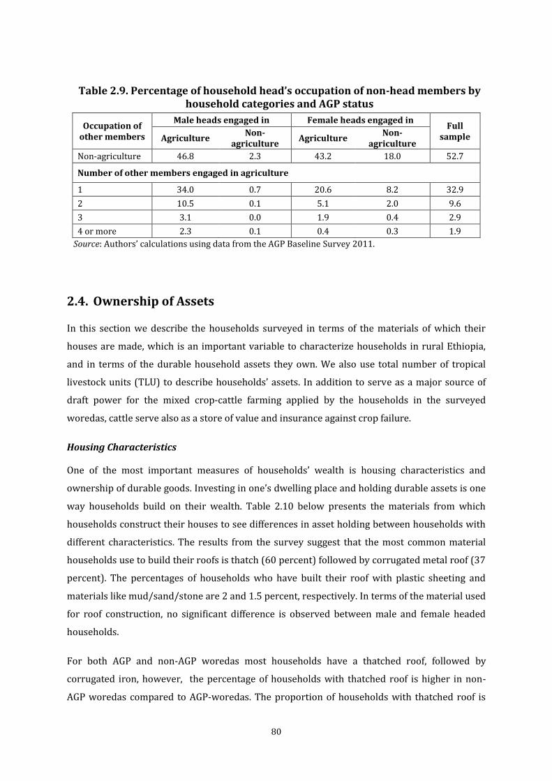
80
Table 2.9. Percentage of household head’s occupation of non-head members by household categories and AGP status
Occupation of other members
Male heads engaged in Female heads engaged in Full
sample Agriculture Non-
agriculture Agriculture
Non-agriculture
Non-agriculture 46.8 2.3 43.2 18.0 52.7
Number of other members engaged in agriculture
1 34.0 0.7 20.6 8.2 32.9
2 10.5 0.1 5.1 2.0 9.6
3 3.1 0.0 1.9 0.4 2.9
4 or more 2.3 0.1 0.4 0.3 1.9
Source: Authors’ calculations using data from the AGP Baseline Survey 2011.
2.4. Ownership of Assets
In this section we describe the households surveyed in terms of the materials of which their
houses are made, which is an important variable to characterize households in rural Ethiopia,
and in terms of the durable household assets they own. We also use total number of tropical
livestock units (TLU) to describe households’ assets. In addition to serve as a major source of
draft power for the mixed crop-cattle farming applied by the households in the surveyed
woredas, cattle serve also as a store of value and insurance against crop failure.
Housing Characteristics
One of the most important measures of households’ wealth is housing characteristics and
ownership of durable goods. Investing in one’s dwelling place and holding durable assets is one
way households build on their wealth. Table 2.10 below presents the materials from which
households construct their houses to see differences in asset holding between households with
different characteristics. The results from the survey suggest that the most common material
households use to build their roofs is thatch (60 percent) followed by corrugated metal roof (37
percent). The percentages of households who have built their roof with plastic sheeting and
materials like mud/sand/stone are 2 and 1.5 percent, respectively. In terms of the material used
for roof construction, no significant difference is observed between male and female headed
households.
For both AGP and non-AGP woredas most households have a thatched roof, followed by
corrugated iron, however, the percentage of households with thatched roof is higher in non-
AGP woredas compared to AGP-woredas. The proportion of households with thatched roof is

81
higher for young household heads compared to households with mature heads; more
households with mature heads have corrugated metal as roof material compared to households
with young heads.
Table 2.10. Percentage of household head’s that used different materials to construct their dwelling by household categories and AGP status
Group Category
Roof Floor
Plastic sheeting
Thatched Mud/ sand/
stone, etc.
Corrugated metal
Earth Cow dung
mixed with soil
Concrete/stone/ cement
Tile
National
All HHs 1.9 59.7 1.5 36.9 62.1 37.2 0.5 0.1
Female HHHs 2.0 67.1 1.6 29.3 62.5 36.9 0.5 0.04
Male HHHs 1.8 56.5 1.5 40.2 62.0 37.4 0.5 0.2
Mature HHHs 1.6 56.9 1.6 39.9 61.8 37.4 0.7 0.1
Youth HHHs 2.4 64.4 1.4 31.8 62.6 37.0 0.3 0.1
AGP woredas
All HHs 1.4 55.8 1.8 41.0 56.5 42.6 0.8 0.2
Female HHHs 0.9 63.4 1.8 33.9 56.2 43.0 0.6 0.2
Male HHHs 1.6 52.5 1.8 44.1 56.6 42.4 0.8 0.2
Mature HHHs 1.1 54.2 1.9 42.7 57.4 41.6 0.8 0.2
Youth HHHs 1.8 58.4 1.7 38.0 54.9 44.3 0.7 0.1
Non-AGP woredas
All HHs 2.0 60.9 1.4 35.6 63.9 35.6 0.4 0.1
Female HHHs 2.3 68.3 1.6 27.8 64.4 35.0 0.5
Male HHHs 1.9 57.7 1.4 39.0 63.6 35.8 0.4 0.2
Mature HHHs 1.7 57.7 1.5 39.0 63.2 36.1 0.6 0.1
Youth HHHs 2.5 66.2 1.3 30.0 64.9 34.8 0.1 0.2
Source: Authors’ calculations using data from the AGP Baseline Survey 2011. Note: ‘HHHs’ and ‘HHs’ stands respectively for ‘headed households’ and ‘households’
In terms of floor material, 62 percent of the households have not made any construction to
improve their floor while 37 percent have cow dung mixed with soil as floor material. The
proportion of households with concrete/stone/cement and tile as floor material are only 0.5
and 0.1 percent, respectively. No significant difference is observed in the floor material of
houses of male and female headed households. A higher proportion of households in AGP
woredas have an improved floor material compared to those in non-AGP woredas. In other
words, the percentage of households with earth as floor material is lower for AGP woredas
while the percentage of those with cow dung mixed with soil is higher for those in AGP woredas.
Durable Household Assets
Table 2.11 presents ownership of durable household assets by farm households. As indicated in
the table below, ownership of bed stood first (34.6 percent) in terms of percentage followed by
TV/radio and jewellery. The survey result revealed that male headed farmers acquire a larger
percentage share of non-productive assets than their female counterparts. Very few households

82
own a car. Assets such as radio/TV and mobile are used to obtain information. However, very
small proportions of households (13 percent) possess mobile phones. Considering households
across AGP and non-AGP woredas, the results show that households in AGP woredas own more
durable household assets than their counterparts in non-AGP woredas.
Table 2.11. Percentage of household head’s asset ownership structure by household categories and AGP status
Group Category Stove Sofa Bed Mobile Radio/
Television Jewellery
Table/ chair
Wheel-barrow
cart Car
National
All HHS 13.4 3.3 34.6 13.1 30.2 22.2 8.6 3.9 1.6
Female HHHs 10.9 1.9 25.3 8.2 17.7 13.3 4.5 2.5 0.9
Male HHHs 14.5 3.9 38.6 15.3 35.6 26.0 10.3 4.5 1.9
Mature HHHs 13.7 3.5 35.2 12.2 28.7 20.5 8.7 3.9 2.0
Youth HHHs 13.0 2.9 33.6 14.6 32.7 25.1 8.4 3.9 0.9
AGP woredas
All HHS 20.3 4.0 38.7 12.9 31.3 25.9 7.5 3.6 1.0
Female HHHs 18.1 3.2 33.3 9.0 19.1 18.2 5.3 2.5 1.0
Male HHHs 21.3 4.4 41.1 14.7 36.6 29.3 8.5 4.1 1.0
Mature HHHs 21.0 4.3 39.5 12.4 30.8 22.7 7.1 3.6 1.1
Youth HHHs 19.2 3.5 37.4 13.9 32.1 31.5 8.4 3.6 0.9
Non-AGP woredas
All HHS 11.3 3.0 33.3 13.2 29.9 21.0 8.9 4.0 1.8
Female HHHs 8.6 1.5 22.8 8.0 17.2 11.7 4.3 2.6 0.8
Male HHHs 12.4 3.7 37.8 15.4 35.3 25.0 10.9 4.6 2.2
Mature HHHs 11.3 3.3 33.8 12.2 28.0 19.7 9.2 4.0 2.3
Youth HHHs 11.2 2.6 32.4 14.8 32.9 23.1 8.4 4.0 0.9
Source: Authors’ calculations using data from the AGP Baseline Survey 2011. Note: ‘HHHs’ and ‘HHs’ stand respectively for ‘Headed Households’ and ‘Households’.
Ownership of Livestock
In addition to the flow of draft power services they provide, cattle also serve as a store of value.
In fact there are parts of Ethiopia in which cattle are the only measure of household wealth.
Tropical livestock units (TLU) are the standardised unit of choice in measuring livestock
holding.8 Accordingly, an average household in the surveyed woredas owned 3.75 cattle of
different ages and sexes, 2.32 sheep and goats, 0.65 pack animals, and 0.002 camels, while the
average number of TLU owned is 3.29. Disaggregating the number of cattle into their age and
sex categories, an average household owned about 1.6 calves, young bulls, and heifers, 0.18
bulls, 0.97 oxen, and 1.01 cows, respectively.
An average female headed household owned fewer livestock of all types relative to an average
male headed household, with the latter owning 37 percent more cattle, 21 percent more shoats
8Tropical livestock unit is often used to standardize the value of different types of cattle into camel units. The formula used to convert cattle into TLU is: TLU= total cattle*0.7+total sheep*0.1+total goats*0.1+total horse*0.8+total asses*0.5+total mules*0.7+ total camel
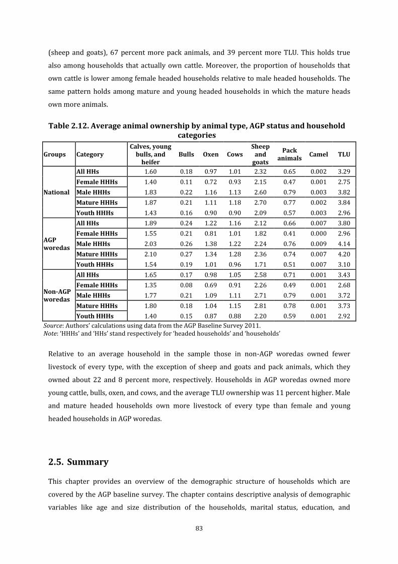
83
(sheep and goats), 67 percent more pack animals, and 39 percent more TLU. This holds true
also among households that actually own cattle. Moreover, the proportion of households that
own cattle is lower among female headed households relative to male headed households. The
same pattern holds among mature and young headed households in which the mature heads
own more animals.
Table 2.12. Average animal ownership by animal type, AGP status and household categories
Groups Category Calves, young
bulls, and heifer
Bulls Oxen Cows Sheep
and goats
Pack animals
Camel TLU
National
All HHs 1.60 0.18 0.97 1.01 2.32 0.65 0.002 3.29
Female HHHs 1.40 0.11 0.72 0.93 2.15 0.47 0.001 2.75
Male HHHs 1.83 0.22 1.16 1.13 2.60 0.79 0.003 3.82
Mature HHHs 1.87 0.21 1.11 1.18 2.70 0.77 0.002 3.84
Youth HHHs 1.43 0.16 0.90 0.90 2.09 0.57 0.003 2.96
AGP woredas
All HHs 1.89 0.24 1.22 1.16 2.12 0.66 0.007 3.80
Female HHHs 1.55 0.21 0.81 1.01 1.82 0.41 0.000 2.96
Male HHHs 2.03 0.26 1.38 1.22 2.24 0.76 0.009 4.14
Mature HHHs 2.10 0.27 1.34 1.28 2.36 0.74 0.007 4.20
Youth HHHs 1.54 0.19 1.01 0.96 1.71 0.51 0.007 3.10
Non-AGP woredas
All HHs 1.65 0.17 0.98 1.05 2.58 0.71 0.001 3.43
Female HHHs 1.35 0.08 0.69 0.91 2.26 0.49 0.001 2.68
Male HHHs 1.77 0.21 1.09 1.11 2.71 0.79 0.001 3.72
Mature HHHs 1.80 0.18 1.04 1.15 2.81 0.78 0.001 3.73
Youth HHHs 1.40 0.15 0.87 0.88 2.20 0.59 0.001 2.92
Source: Authors’ calculations using data from the AGP Baseline Survey 2011. Note: ‘HHHs’ and ‘HHs’ stand respectively for ‘headed households’ and ‘households’
Relative to an average household in the sample those in non-AGP woredas owned fewer
livestock of every type, with the exception of sheep and goats and pack animals, which they
owned about 22 and 8 percent more, respectively. Households in AGP woredas owned more
young cattle, bulls, oxen, and cows, and the average TLU ownership was 11 percent higher. Male
and mature headed households own more livestock of every type than female and young
headed households in AGP woredas.
2.5. Summary
This chapter provides an overview of the demographic structure of households which are
covered by the AGP baseline survey. The chapter contains descriptive analysis of demographic
variables like age and size distribution of the households, marital status, education, and
84
occupation of the household heads and household members. In the discussion, emphasis is also
given to differences between genders, age groups, and AGP status classification.
The average age for the household head is about 43 years while female heads tend to be older.
Regarding marital status of heads, the majority of household heads are married. There are more
female heads who are separated or divorced compared to male heads. However, there is no
notable difference across households in AGP and non-AGP woredas. The surveyed households
have on average five members with relatively smaller size for households with younger heads.
However, there is little difference in household size distribution across AGP classification.
Detailed statistics is also computed across age cohorts.
Regarding the educational status, about 54 percent of the household heads surveyed are
illiterate. When looked across gender, a large majority of the female heads are illiterate, as well
as more than half of the female household members. More young heads had formal education,
while a higher proportion of mature heads had some sort of informal education. Notable
differences also exist among the different age groups.
The occupational structure of households shows that about 89 percent of the household heads
surveyed are farmers or family farm workers and even the proportion reaches about 97 for
male headed households. Female headed households tend to diversify their occupation to non-
agricultural activities a little more.

85
Chapter 3: Characteristics of Crop production and Decision
Making
Almost all households in rural Ethiopia derive their livelihood from agriculture or related
activities. This is true for the millions of households residing in the study area. Among
households included in the sample over 96.6 and 71 percent of male and female heads are
engaged in agriculture, respectively. In households whose livelihood is mainly dependent on
agriculture, it is important to look at the responsible member in decision making of certain
activities.
In the first section of this chapter we describe the importance associated to different crop
categories in terms of the number of plots used and the number of households cultivating them.
In the second section we characterize the households in terms of members responsible for
making decisions on crop and livestock production and use.
3.1. Characteristics of crop production
For the purpose of showing the importance associated to different crops we first describe the
number of plots used to grow the six crop categories of cereals, pulses, oilseeds, vegetables, root
crops, and fruits. The second section describes the number of households growing the crop
categories. Due to the importance in the number of plots used and the number of households
growing enset and coffee, we include them in the description.
Number of Plots by Use
A total of 46.9 million plots were sown to one or more crops or were under permanent crops
during the 2010/11 Meher — the main agricultural season of the year. Out of the total number
of fields 75/25 percent were operated by households with male/female heads, and 65/35
percent by households with matured heads/young heads (Table 3.1). Households in non-AGP
cultivated 75.8 percent of the total amount of plots; households in AGP woredas cultivated the
remaining 24.2 percent of plots. Though the distribution of number of plots by gender and age
slightly varies across AGP and non-AGP woredas, it is generally close to the average in the
overall sample. Relative to the overall sample and non-AGP woredas, fewer plots are operated
by households with female and young heads in AGP woredas.

86
Table 3.1. Number of plots cultivated in Meher 2010/11 by household categories and AGP status
Group Category Number (000) Percent
National
All Households 46,920 100
Male headed Households 35,330 75.3
Female headed Households 11,590 24.7
Youth headed Households 16,383 34.9
Mature headed Households 30,537 65.1
AGP woredas
All Households 11,358 24.2
Male headed Households 8,651 76.2
Female headed Households 2,707 23.8
Youth headed Households 3,862 34.0
Mature headed Households 7,496 66.0
Non-AGP woredas
All Households 35,562 75.8
Male headed Households 26,680 75.0
Female headed Households 8,882 25.0
Youth headed Households 12,521 35.2
Mature headed Households 23,041 64.8
Source: Authors’ calculations using data from the AGP Baseline Survey 2011.
Households have reported to have grown 53 crop types. Ten of the crop types grown are
cereals, 9 are pulses, 5 are oilseeds, 7 are vegetables, 8 are root crops, and 5 are fruits. While we
single out enset and coffee out of the remaining group of relatively heterogeneous crops, the
remaining 7 crops are categorized as “all others”. Out of the total cultivated plots 55 percent
were under cereals, pulses were second in importance at 12.7 percent, with coffee and enset
following at 7.3 and 5.9 percent, respectively. Root crops, oilseeds, fruits, and vegetables were
important in that order and together accounted for about 11.7 percent of the plots (Table 3.2).
The proportion of plots used to grow each of the crop categories differs across male and female
headed households. However, their difference is less than 0.5 percent in all crop categories
except households with male heads allocated 0.9 percent more for cereals. Similarly the
proportion allocated by households with mature and young heads are similar. In general,
households with mature heads allocated relatively more plots to grow pulses and fruit crops
and fewer plots to grow cereals, oilseeds, root crops, and enset. Patterns observed in the
aggregated sample hold across male and female headed and mature and young headed
households in both AGP and non-AGP woredas with few exceptions.

87
Table 3.2. The distribution of plots by crop type, household categories, and AGP status (percent)
Group Category Cereals Pulses Oil
seeds Vegetables Root crops
Fruit crops Coffee Enset
Na
tio
na
l
All HHs 55.3 12.7 3.0 2.0 4.3 2.4 7.3 5.9
Male HHHs 55.5 12.7 3.1 1.9 4.2 2.3 7.4 5.6
Female HHHs 54.6 12.7 2.7 2.4 4.5 2.8 7.1 6.8
Youth HHHs 55.7 12.2 3.2 2.0 4.5 2.2 7.3 6.0
Mature HHHs 55.0 13.0 2.9 2.1 4.2 2.6 7.3 5.8
AG
P w
ore
da
s All HHs 56.2 10.8 3.4 3.1 3.7 2.5 5.0 6.1
Male HHHs 56.3 10.8 3.6 3.0 3.8 2.4 4.9 5.8
Female HHHs 55.6 10.5 2.8 3.4 3.3 2.7 5.3 6.8
Youth HHHs 56.3 9.9 3.5 3.5 4.4 2.5 4.8 6.4
Mature HHHs 56.1 11.2 3.3 2.9 3.3 2.5 5.2 5.9
No
n-A
GP
w
ore
da
s
All HHs 55.0 13.3 2.9 1.7 4.5 2.4 8.0 5.8
Male HHHs 55.2 13.3 2.9 1.6 4.3 2.3 8.1 5.5
Female HHHs 54.3 13.4 2.7 2.0 4.8 2.8 7.6 6.8
Youth HHHs 55.5 13.0 3.2 1.5 4.5 2.1 8.0 5.9
Mature HHHs 54.7 13.5 2.7 1.8 4.4 2.6 8.0 5.8 Source: Authors’ calculations using data from the AGP Baseline Survey 2011. Notes: around 7 % of the plots from the whole sample were allocated for other and mixed crops. ‘HHs’ and ‘HHHs’ stand respectively for ‘Households’ and ‘Headed Households’
Cropping Patterns
Households in the survey planted on average at least two types of crop categories. Table 3.3 lists
the number and proportion of households growing one or more of the 8 important crop
categories/crops. As expected, the largest proportion (about 91 percent) of the households
planted cereals.
Next in importance to cereals are pulses cultivated by 41 percent of the households. Enset and
coffee are close to each other as 3rd and 4th in importance. This ranking of importance holds
across gender and age categories, with the exception that coffee is more important than enset in
female headed households.
The proportion of households growing the different crops in AGP and non-AGP woredas is
mostly similar as discussed in the above paragraph with the most notable exception that enset
is less important than coffee in the non-AGP woredas (but for female headed households in non-
AGP woredas enset is more important than coffee — as opposite to the finding for female
headed households in all households). In addition, vegetables are less important than fruits for
all categories of non-AGP woredas.

88
Table 3.3. Proportion of households growing different crops by household categories and AGP status
Group Category Cereals Pulses Oil
seeds Vegetables Root crops
Fruit crops Coffee Enset
Na
tio
na
l
All HHs 90.57 41.19 11.8 9.51 17.92 8.7 26.02 26.5
Female HHHs 91.66 43.51 13.17 9.58 18.64 8.98 26.77 26.65
Male HHHs 97.98 35.72 8.57 9.35 16.24 8.04 24.25 26.14
Youth HHHs 90.16 38.67 11.86 8.59 17.54 7.71 24.21 25
Mature HHHs 90.81 42.68 11.73 10.06 18.16 9.29 27.09 27.39
AG
P w
ore
da
s All HHs 92.89 33.6 13.67 14.54 16.14 9.24 19.02 27.68
Female HHHs 89.63 28.56 9.72 12.97 12.6 8.54 18.48 26.19
Male HHHs 94.25 35.69 15.31 15.2 17.62 9.52 19.25 28.31
Youth HHHs 92.32 31.78 13.44 15.01 17.26 8.59 16.51 27.02
Mature HHHs 93.22 34.64 13.79 14.28 15.51 9.6 20.45 28.07
No
n-A
GP
w
ore
da
s
All HHs 89.85 43.52 11.22 7.97 18.47 8.54 28.17 26.13
Female HHHs 87.49 37.88 8.23 8.26 17.34 7.89 25.99 26.13
Male HHHs 90.86 45.93 12.5 7.84 18.95 8.81 29.1 26.14
Youth HHHs 89.51 40.72 11.38 6.68 17.62 7.45 26.49 24.4
Mature HHHs 90.06 45.2 11.13 8.74 18.98 9.19 29.17 27.18
Source: Authors’ calculations using data from the AGP Baseline Survey 2011. Note: ‘HHHs’ and ‘HHs’ stands respectively for ‘Headed households and ‘households’
3.2. Decision Making in Agriculture
In this section we describe patterns in decision making for production of both crops and
livestock and livestock products. To that end we use three aspects of decision making in
agricultural production: types of crop to produce, how to market crop outputs, and production
of livestock and livestock products. We provide the number and proportion of households in
which different members are responsible for making decision on which crop to produce and on
marketing of output in Tables 3.4 and 3.5, respectively, while Table 3.6 summarizes production
decision for livestock and livestock products.
Table3.4 shows proportion of household members that make decision on what to plant. In most
households it is the head that most often makes production and consumption decisions. In 72
percent of the surveyed households it is the head who decide what corps to plant, in 86 percent
of the households the head decides how to market crop output, and in 92 percent of the
households he/she determines which livestock to keep (Tables 3.4-3.6). It is interesting to note
that in 21 percent of the households decisions on what crop to produce are jointly decided by
the head and spouse. The proportion of households in which the spouse is responsible in
deciding what crop to produce, 3.5 percent, is about the same as the proportion in which adult
children make the decision alone or jointly with the head and the spouse, which is about 3.6
percent.

89
There are remarkable differences between households with male and female heads. In 69.6
percent of the male headed households the head decides what crop to plant while this
proportion is larger among female headed households with 79.6 percent. By contrast, the
proportion in which the head and spouse make the decision jointly is much larger among male
headed households at 26 percent relative to the 4.7 percent in female headed households. This
is largely because only 31 percent of the female heads are married, compared to 94 percent of
the male heads.
In both young and mature headed households most decision on crop planting are made by the
head. One remarkable difference is that in more decisions on are made by both head and spouse
in young headed households (i.e., 23.2 percent) than in mature headed households (i.e., 19.3
percent). To the contrary, in households with mature heads a larger proportion of adult children
make a decision (i.e., 5.1 percent), compared to adult children in households with young heads
(i.e., 0.6 percent).
The decision making pattern in non-AGP woredas differs only slightly from the average for the
overall sample, with slightly fewer heads but slightly more heads and spouses making the
decisions. The exact opposite of this holds among AGP households.
Table 3.4. Household members that make decision on what crop to plant by AGP status
Group Category Head Spouse
Head and
spouse Adult
children
Head and adult
children
Spouse and adult children
National
All HHs 72.3 3.5 20.6 1.2 1.8 0.6
Male HHHs 69.6 3.1 26.2 0.2 0.2 0.7
Female HHHs 79.9 4.7 4.7 4.1 6.4 0.1
Youth HHHs 72.0 4.1 23.2 0.2 0.4 0.03
Mature HHHs 72.4 3.2 19.3 1.7 2.5 0.9
AGP woredas
All HHs 75.7 3.9 17.8 0.8 1.6 0.3
Male HHHs 73.6 3.8 22.1 0.1 0.2 0.3
Female HHHs 82.1 4.2 4.5 3.1 5.8 0.4
Youth HHHs 76.3 3.8 19.2 0.1 0.5 0.1
Mature HHHs 75.4 3.9 17.1 1.1 2.1 0.4
Non-AGP woredas
All HHs 71.3 3.4 21.5 1.3 1.9 0.7
Male HHHs 68.4 2.9 27.4 0.2 0.2 0.9
Female HHHs 79.2 4.9 4.8 4.4 6.6 0.1
Youth HHHs 70.8 4.2 24.4 0.3 0.4 0.02
Mature HHHs 71.5 2.9 20 1.9 2.7 1
Source: Authors’ calculations using data from the AGP Baseline Survey 2011. Note: ‘HHHs’ and ‘HHs’ stands respectively for ‘Headed households’ and ‘households’
Table 3.5 presents the percentage of household members who make decisions on the marketing

90
of crop products. For 86 percent of the households, household heads are the sole deciders on
issues related with crop marketing while the spouse makes such decision in only 8 percent of
the households. In comparing male and female headed households, a higher proportion of
female heads make the marketing decisions while decisions by the spouse are more prevalent in
the male headed households. When compared to mature headed households, a higher
percentage of marketing decisions in young headed households are made by household heads.
In AGP woredas more decisions are made by the head or spouse, and less are made by the
children, than in the non-AGP woredas. This pattern is also observed when looking into the
different household categories within households in AGP and non-AGP woredas.
Table 3.5. Household members that make decision on marketing of crop by household categories and AGP status
Group Category Head Spouse Child Other
National
All HHs 86.43 8.13 4.58 0.86
Male HHHs 85.18 10.59 3.8 0.43
Female HHHs 90.13 0.86 6.9 2.11
Youth HHHs 89.46 7.65 2.24 0.65
Mature HHHs 84.64 8.42 5.97 0.97
AGP woredas
All HHs 87.49 9.13 2.44 0.94
Male HHHs 85.85 11.77 1.92 0.46
Female HHHs 92.5 1.09 4.03 2.38
Youth HHHs 89.96 8.06 1.56 0.42
Mature HHHs 86.11 9.73 2.93 1.23
Non-AGP woredas
All HHs 86.06 7.78 5.34 0.82
Male HHHs 84.94 10.17 4.47 0.42
Female HHHs 89.33 0.78 7.88 2.01
Youth HHHs 89.3 7.51 2.47 0.72
Mature HHHs 84.11 7.94 7.06 0.89
Source: Authors’ calculations using data from the AGP Baseline Survey Note: ‘HHHs’ and ‘HHs’ stands respectively for ‘Headed households’ and ‘households’
In what looks like an extension of the decision on crop to cultivate, the number and type of
livestock that a household keeps is decided by the head in an even larger proportion of
households. While this is true for most livestock in about 91 percent of the households, it is
markedly lower for chickens at 68 percent, in which the spouse makes the decision in 24
percent of the households. The proportion of female heads that make the decision on the
number of chickens to keep is larger at 92.5 percent. In male headed households the decision on
how to use milk and milk products is decided by the spouse while in female headed households
it is the head that makes such decision, which together imply that such decisions are made by
female spouses or female heads.

91
Table 3.6. Proportion of household members that make decisions on livestock and livestock products by household head categories
Category
Cattle Goats & Sheep Pack Animals Chicken
Head Spouse Child Head Spouse Child Head Spouse Child Head Spouse Child
All HHs 91.6 2.8 4.4 90.5 2.7 4.8 90.9 0.8 5.5 67.8 24.3 6.4
Male HHHs 92.2 3.3 3.5 92.9 3.1 3.2 91.7 0.9 5.7 58.2 33.1 7.2
Female HHHs 89.6 1.3 7.3 84 1.3 9.4 86 0 4.4 92.5 1.7 4.5
Youth HHHs 90.6 3.5 4.3 91.5 3.3 3.5 88.9 0.1 7.4 67.1 26.3 3.4
Mature HHHs 92.3 2.4 4.4 89.9 2.3 5.6 92.2 1.3 4.3 68.3 22.8 8.6
Milk Cheese Butter Yoghurt
Head Spouse Child Head Spouse Child Head Spouse Child Head Spouse Child
All HHs 26.5 65.62 1.11 34.16 56.61 0 31 62.8 3.11 71.21 28.79 0
Male HHHs 4.23 90.62 0 10.63 80.1 0 6.8 88.24 1.59 26.86 73.14 0
Female HHHs 84.97 0 4.03 90.85 0 0 90.55 0.22 6.85 100 0 0
Youth HHHs 19.11 73.38 1.11 37.18 58.87 0 36.15 57.62 3.86 95.17 4.83 0
Mature HHHs 36.47 55.17 1.11 27.79 51.85 0 22.07 71.79 1.82 29.14 70.86 0
Source: Authors’ calculations using data from the AGP Baseline Survey 2011. Note: ‘HHHs’ and ‘HHs’ stand respectively for ‘Headed households’ and ‘households’
3.3. Summary
The chapter summarises crop allocation and decision making of households in the production
and sale of crop and livestock products. In the surveyed households, the total number of plots
cultivated for Maher season was 46.9 million. A significant percentage of variation was observed
in the proportion of plots allocated for each crop categories. Cereals took the largest proportion
of plots used for production, followed by pulses and coffee. This result holds true for AGP and
non-AGP woredas, except in AGP woredas enset is more important than coffee. Decision making
on crop production was almost always made by the head and head and spouse. Likewise,
decision on marketing of crop produced is mostly done by the head and followed by the spouse
though the percentage is much lower than the proportion of the head. Decisions on the number
and type of livestock that a household keeps is decided by the head, however, for chickens heads
do decide in most cases, but the proportion of households in which the spouses make the
decision is markedly larger than for other livestock types. A noticeable result was found
regarding the decision making on the production of milk and milk products; these decisions are
made by the female spouses and female heads.

92
Chapter 4: Productivity in Agriculture
Enhancing smallholders’ productivity, via improvements in input provision and market access,
is the central objective of AGP. Tracking indicators of crop productivity is thus a key component
of monitoring progress and impact associated with AGP. The AGP baseline survey collected data
on household-level quantity of output produced and inputs applied for that purpose. The
information obtained is subsequently used to generate estimates of the desired productivity
indicators. This chapter reports on output levels, yields, and labour productivity estimates for
both crop and, to a more limited extent, livestock production.
4.1. Productivity in the Crop Sub-sector
Land Productivity
A recap on the composition of crop output is provided as a prelude. That is followed by a brief
look at reported output levels and plot sizes. All of these are helpful dimensions that
contextualize subsequent analysis of yields.
More than fifty types of crops were cultivated by farmers covered by the baseline during Meher
2010/11 (see chapter 3 for more details). Such diversity makes both analysis and interventions
rather challenging. For the purpose of the descriptive analysis, these crops are categorised into
fifteen groups — Teff, Barley, Wheat, Maize, Sorghum, Other Cereals, Pulses, Oilseeds,
Vegetables, Fruits, Root Crops, Coffee, Chat, Enset, Others.9 Figure 4.1 summarizes the share of
these groups in total cultivated area and total grain output (measured as an un-weighted
physical sum over output of individual crops).
Figure 4.1 Shares in cultivated area and grain output
Source: Authors’ calculations using data from the AGP Baseline Survey 2011.
9 In subsequent sections ‘Other Cereals’ are frequently combined with ‘Others’.

93
The first striking feature conveyed by the figure is the predominance of cereals — thus
justifying the inclusion of five single cereals as distinct groups. All cereals together accounted
for 66 percent of acreage. Among the cereals, teff (16.1 percent) recorded the largest share of
cultivated area, followed closely by maize (15.2 percent) and wheat (11.5 percent). As a group,
pulses took 16 percent of area cultivated, thereby bringing the share of grains to a total of 85.6
percent (with oilseeds also included). Fruits (3.8 percent), root crops (3.7 percent), and oil
seeds (3.6 percent) made up the other major non-cereal crop categories with significant shares.
The acreage share of enset is only 1.6 percent.
It is noteworthy that teff, having the largest acreage share, did not make it the top contributor of
grain output. It only reached third place with 13 percent. With 30 percent, maize had by far the
largest share in grain output, while wheat (17 percent) had the second largest.
There is some variation across AGP and non-AGP woredas in terms of crop shares in cultivated
area. On average, AGP woredas had larger acreage shares going to teff, sorghum, and oil seeds
(see Annex Figure B.4.1). In contrast, non-AGP woredas recorded greater shares to barley,
maize, pulses, and coffee. The two sub-samples had essentially the same shares for the other
crops.
Output Levels
Table 4.1 reports average Meher output levels estimated from the AGP baseline data. For each
crop, the estimates are based on declared output levels of households who have reported to be
engaged in the production of that crop. The estimates reveal that average levels of output per
household are not very high. At the national level, they range from 1.3 quintals for coffee
through to 5.8 quintals for maize. Even lower numbers are observed if the median is considered
instead of the mean. For instance, the overall mean output of teff-producing households was 3.1
quintals. The median, on the other hand, is 2 quintals, implying that half of these households
produced less than 2 quintals. In addition, as expressed by the standard deviations included in
the table, the average levels hide considerable variation across households. Figure 4.2 presents
a more visual way of summarising this variation. It plots the mean levels of output per
household by output quintiles for the five major cereals. Households in the bottom quintile
(Quintile I) on average produced less than a quintal for all the cereals, while those in the top
quintile (Quintile V) managed to produce a much higher average output, i.e., 8 quintals for teff
through to 18 quintals for sorghum. Annex Figures B.4.2 and B.4.3 show that comparable
differences were also prevalent in relation to other crops as well as within AGP and non-AGP
woredas.

94
Table 4.1. Average output (quintals), by AGP status and household head characteristics
Group Category Statistic Teff Barley Wheat Maize Sorghum Pulses Oil Seeds
Vege tables
Root Crops
Fruit Crops Chat Coffee Enset
National
All HHs
Mean 3.1 4.3 5 5.8 5.2 1.7 1.7 2.7 4.8 1.5 1.8 1.3 3.8
Median 2 2.8 2.8 3 3 1 1 1 2.1 0.3 0.4 0.5 1.5
SD 3.7 4.8 7.5 9.8 7.3 2 2.5 5.0 7.6 7.3 6.1 2.1 7.8
Male HHHs
Mean 3.4 4.4 5.2 6.6 5.8 1.8 1.8 2.8 5.4 1.1 1.9 1.2 4
Median 2 2.5 2.8 3 3 1 1 1 2.5 0.2 0.4 0.5 1.5
SD 4 5 7.7 11 8 2.2 2.6 5.4 8.5 3.8 6.8 2.1 8.5
Female HHHs
Mean 2.4 4 4.5 3.8 3.6 1.4 1.4 2.6 3.5 2.6 1.3 1.3 3.2
Median 2 3 2.1 2 2 1 1 1 2 0.5 0.3 0.5 1
SD 2.3 4.1 6.9 5.8 4.5 1.5 2.2 3.6 4.3 12 2.6 2 5.9
Mature HHHs
Mean 3.2 4.2 5 5.8 5.3 1.7 1.7 2.7 4.9 1.5 1.8 1.3 3.8
Median 2 2.8 2.8 3 3 1 1 1 2.1 0.3 0.4 0.5 1.5
SD 3.7 4.8 7.6 9.9 7.4 2 2.6 5 7.8 7.5 6.1 2.1 8.0
Youth HHHs
Mean 2.7 4.5 4.6 5.6 4.6 1.6 1.7 2.4 4 1 1.6 0.9 2.7
Median 2 3 2.5 3 2 1 1 1 2.8 0.4 0.5 0.5 1.5
SD 2.3 4.5 5.5 7.3 5.9 1.7 2.2 4 4 1.6 6 1 4
AGP woredas
All HHs
Mean 3.4 4.1 5.4 5 7.5 2.2 3.1 2.5 4.6 1.3 2.7 1.3 3.6
Median 2.5 2.4 2.8 2.5 5 1.5 2 1 2 0.2 0.6 0.5 1.5
SD 3.6 5 8 7.9 8.8 2.5 4.2 5 8.3 5.9 6.9 2.8 7.3
Male HHHs
Mean 3.6 4.1 5.6 5.4 8.3 2.2 3.2 2.4 5 1.5 2.9 1.4 3.6
Median 2.5 2.3 3 3 5 1.5 2 1 2.1 0.2 0.6 0.5 1.5
SD 3.8 5.1 8.4 7.2 9.4 2.6 4.2 5 9.1 6.8 7.6 3 7.2
Female HHHs
Mean 2.8 3.9 4.8 3.9 5.3 2.1 2.6 2.6 3.4 0.9 2.3 1.1 3.6
Median 2 2.4 2.5 2 4 1.5 1.5 1 2 0.2 0.6 0.5 1.5
SD 2.9 4.5 6.6 9.4 6.1 2.3 3.8 4.7 4.4 2.2 4 2.4 7.4
Mature HHHs
Mean 3.5 4.1 5.4 5 7.6 2.2 3.1 2.5 4.7 1.3 2.7 1.3 3.6
Median 2.5 2.4 2.8 2.5 5 1.5 2 1 2 0.2 0.6 0.5 1.5
SD 3.6 5 8 8 8.8 2.5 4.2 4.9 8.5 6.1 6.6 2.9 7.3
Youth HHHs
Mean 2 3.6 5.6 5 6.5 2 2.8 1.5 2.6 1.3 3.7 0.8 3.5
Median 1.5 2.8 3 2.8 4 1.5 2 0.5 1 0.2 0.2 0.3 1
SD 2 3.2 8.1 6.3 8.3 2.9 3.2 5.3 3.4 2.3 11 1.3 6.6
Non-AGP woredas
All HHs
Mean 3.4 4.1 5.4 5 7.5 2.2 3.1 2.5 4.6 1.3 2.7 1.3 3.6
Median 2.5 2.4 2.8 2.5 5 1.5 2 1 2 0.2 0.6 0.5 1.5
SD 3.6 5 8 7.9 8.8 2.5 4.2 5 8.3 5.9 6.9 2.8 7.3
Male HHHs
Mean 3.3 4.4 5.1 6.9 4.9 1.8 1.2 2.9 5.5 0.9 1.6 1.2 4.1
Median 2 2.8 2.8 3 2.5 1 0.8 1 2.5 0.2 0.4 0.5 1.5
SD 4.1 5 7.5 12 7.2 2 1.1 5.6 8.3 1.9 6.4 1.8 8.9
Female HHHs
Mean 2.1 4 4.4 3.8 3 1.2 0.9 2.6 3.5 3.1 0.9 1.4 3.1
Median 1.8 3 2 2.1 1.8 0.8 0.8 1.4 2 0.5 0.2 0.5 1
SD 1.9 4 7 4.3 3.6 1.2 0.6 3.1 4.3 14 1.7 1.9 5.4
Mature HHHs
Mean 3 4.3 4.9 6 4.4 1.6 1.1 2.8 4.9 1.6 1.5 1.3 3.9
Median 2.0 2.8 2.5 3 2 1 0.8 1 2.1 0.3 0.3 0.5 1.4
SD 3.8 4.7 7.5 10 6.6 1.9 1 5 7.6 7.9 5.9 1.9 8.2
Youth HHHs
Mean 2.9 4.7 4.3 5.8 3.6 1.5 1.1 2.9 4.4 0.9 0.8 0.9 2.4
Median 2.0 4 2.1 3 2 1 0.5 2 3.5 0.4 0.5 0.5 1.5
SD 2.4 4.7 4.5 7.6 3.8 1.4 1.2 3 4.2 1.2 0.7 0.9 2.7
Source: Authors’ calculations using data from the AGP Baseline Survey 2011. Notes: HHHs and HHs stand respectively for ‘Headed Households’ and ‘Households’. SD denotes ‘Standard Deviation’.

95
As can be seen from Table 4.1 some of this heterogeneity is correlated with household location
as well as gender and age differences among household heads. Among the crops considered,
average household output was higher in AGP woredas relative to non-AGP woredas for teff,
wheat, maize, sorghum, pulses, oil seeds, and chat. Average output was greater in non-AGP
woredas for the other crops. However, the only statistically significant differences were the
bigger output levels for sorghum, pulses, and oilseeds in AGP woredas (see Annex Table
B.4.1).10 The gender of the household head is another important correlate. Male headed
households reported higher output levels in almost all crops, and we found statistically
significant ones for six crops (Annex Table B.4.1). These differences largely persist across AGP
and non-AGP woredas. In contrast, age of the household head appears not to matter much,
except for coffee production (mature heads reporting higher levels of coffee output).
Figure 4.2. Average household cereal production in kg, by output quintiles
Source: Authors’ calculations using data from the AGP Baseline Survey 2011.
Average Plot Size
Plot sizes are briefly considered to complement the perspective provided by average output
levels reported on above.
Table 4.2 reveals that plot sizes were not large in the study areas. Average plot sizes hover
around a third of a hectare. Moreover, no significant difference in average plot size can be
detected across annual crops, though sorghum and oilseeds had the two highest average plot
sizes. Both features are consistent with the usual characterization of the farmers covered by the
survey as smallholders. Looking across household types, it is notable that male headed
10
Roughly speaking, statistically significant differences are those which are more than a chance occurrence.

96
households have slightly bigger plots compared to female headed households. So did mature
headed households relative to young headed households. Significant size differences were
observed within crops, however. Calculated standard deviations are high, particularly relative
to the averages. There are really tiny plots as there are much-larger-than-average plots. As the
next section reveals, this considerable variation in plot size has implications for yield estimates.
Table 4.2. Average plot size (ha), by crop type
Group Category Statistic Teff Barley Wheat Maize Sorghum Pulses Oil
Seeds Vege
tables Root
Crops Fruit Crops Chat Coffee Enset
National
All HHHs Mean 0.3 0.28 0.29 0.27 0.38 0.22 0.36 0.21 0.21 0.24 0.2 0.2 0.2
SD 0.29 0.38 0.29 0.45 0.36 0.31 0.43 0.68 0.55 0.61 0.4 0.4 0.4
Female HHHs
Mean 0.28 0.28 0.28 0.24 0.33 0.21 0.33 0.17 0.3 0.3 0.2 0.2 0.2
SD 0.22 0.35 0.25 0.38 0.28 0.34 0.32 0.54 0.7 0.9 0.4 0.4 0.4
Male HHHs
Mean 0.31 0.28 0.3 0.28 0.39 0.22 0.36 0.23 0.19 0.2 0.2 0.2 0.2
SD 0.3 0.39 0.3 0.47 0.38 0.3 0.46 0.73 0.48 0.45 0.4 0.4 0.3
Mature HHHs
Mean 0.3 0.28 0.29 0.28 0.38 0.22 0.36 0.22 0.21 0.21 0.2 0.2 0.2
SD 0.29 0.39 0.29 0.45 0.36 0.31 0.44 0.69 0.56 0.43 0.4 0.4 0.4
Youth HHHs
Mean 0.29 0.27 0.31 0.21 0.31 0.18 0.34 0.11 0.2 0.78 0.2 0.3 0.3
SD 0.25 0.25 0.24 0.24 0.25 0.15 0.28 0.24 0.29 1.78 0.3 0.4 0.3
AGP woredas
All HHHs Mean 0.33 0.28 0.29 0.25 0.53 0.22 0.53 0.18 0.21 0.23 0.2 0.3 0.2
SD 0.32 0.27 0.31 0.35 0.48 0.27 0.59 0.59 0.54 0.6 0.5 0.5 0.4
Female HHHs
Mean 0.28 0.26 0.32 0.22 0.45 0.22 0.48 0.15 0.17 0.27 0.2 0.2 0.2
SD 0.24 0.24 0.3 0.3 0.39 0.23 0.52 0.51 0.26 0.73 0.6 0.5 0.3
Male HHHs
Mean 0.34 0.28 0.29 0.26 0.56 0.22 0.55 0.19 0.22 0.22 0.2 0.3 0.2
SD 0.33 0.28 0.31 0.36 0.49 0.28 0.6 0.62 0.59 0.55 0.5 0.5 0.4
Mature HHHs
Mean 0.33 0.28 0.29 0.25 0.54 0.22 0.54 0.18 0.2 0.2 0.3 0.3 0.2
SD 0.32 0.26 0.31 0.35 0.48 0.27 0.6 0.6 0.6 0.6 0.5 0.5 0.4
Youth HHHs
Mean 0.3 0.36 0.33 0.25 0.42 0.26 0.47 0.13 0.15 0.48 0.2 0.3 0.2
SD 0.27 0.46 0.3 0.36 0.37 0.23 0.41 0.34 0.14 1.01 0.3 0.7 0.3
Non-AGP woredas
All HHHs Mean 0.29 0.28 0.29 0.28 0.32 0.21 0.29 0.23 0.2 0.2 0.2 0.2 0.2
SD 0.27 0.4 0.28 0.47 0.29 0.32 0.34 0.73 0.6 0.6 0.3 0.3 0.3
Female HHHs
Mean 0.28 0.26 0.32 0.22 0.45 0.22 0.48 0.15 0.17 0.27 0.2 0.2 0.2
SD 0.24 0.24 0.3 0.3 0.39 0.23 0.52 0.51 0.26 0.73 0.6 0.5 0.3
Male HHHs
Mean 0.34 0.28 0.29 0.26 0.56 0.22 0.55 0.19 0.22 0.22 0.2 0.3 0.2
SD 0.33 0.28 0.31 0.36 0.49 0.28 0.6 0.62 0.59 0.55 0.5 0.5 0.4
Mature HHHs
Mean 0.29 0.28 0.29 0.29 0.33 0.22 0.29 0.24 0.21 0.2 0.2 0.2 0.2
SD 0.28 0.41 0.28 0.48 0.29 0.32 0.34 0.74 0.56 0.38 0.3 0.3 0.3
Youth HHHs
Mean 0.28 0.26 0.3 0.2 0.25 0.17 0.29 0.09 0.22 0.91 0.3 0.3 0.3
SD 0.24 0.22 0.22 0.19 0.14 0.13 0.2 0.1 0.32 2.08 0.4 0.3 0.3
Source: Authors’ calculations using data from the AGP Baseline Survey 2011. Notes: HHHs and HHs stand respectively for ‘Headed Households’ and ‘Households’.

97
Crop Yields
Land productivity is usually measured by yield or output per hectare (or other units of land).
Yield is also the primary indicator identified with AGP’s objective of raising agricultural
productivity. This subsection reports on yield measured as reported farm households’ crop
output per hectare of land cultivated. The discussion is confined to the major cereals (teff,
barley, wheat, maize, and sorghum), pulses, oil seeds, root crops, enset, and coffee. Vegetables,
fruits, and chat are thus not considered
Table 4.3. Average crop yield (quintal/ha)1, by household head characteristics
Category Statistic Teff Barley Wheat Maize Sorghum Pulses
Oil Seeds
Root Crops
Chat Enset Coffee
Na
tio
na
l
All HHs
Mean 9.4 14.7 14.6 17.2 11.5 10.9 5.1 46.6 130.6 52.3 12.1
Median 6.7 9.6 10.0 12.0 8.0 6.7 4.0 24.0 4.7 10.0 3.4
SD 9.0 14.8 14.4 17.4 10.4 14.2 5.8 64.5 677.9 203.3 40.4
Female HHHs
Mean 8.4 13.4 13.3 15.5 9.9 10.1 5.0 32.9 160.9 58.5 10.7
Median 6.0 8.4 10.0 11.4 8.0 6.0 4.0 22.4 2.7 8.0 4.1
SD 8.2 12.5 12.5 14.9 8.5 15.6 4.7 37.4 700.3 233.4 28.9
Male HHHs
Mean 9.7 15.1 15.0 17.9 12.0 11.1 5.2 51.9 122.1 49.7 12.6
Median 7.3 10.0 10.0 12.0 8.8 7.0 4.0 25.0 5.6 10.0 3.3
SD 9.2 15.5 14.9 18.3 10.9 13.8 6.0 71.6 671.2 188.9 43.7
Mature HHHs
Mean 9.3 14.6 14.4 17.1 11.6 10.8 5.1 45.2 118.3 57.6 13.1
Median 6.6 9.3 10.0 11.2 8.2 6.4 4.0 24.0 4.0 10.0 3.3
SD 8.8 14.4 14.0 17.4 10.0 14.9 5.8 61.3 722.4 219.9 43.7
Youth HHHs
Mean 9.6 14.8 14.8 17.5 11.2 11.0 5.1 49.2 153.7 42.6 10.0
Median 7.0 9.6 9.6 12.1 8.0 7.0 4.0 24.0 8.0 10.0 3.4
SD 9.4 15.4 14.9 17.5 10.9 13.0 5.7 70.0 584.3 168.0 32.7
Source: Authors’ calculations using data from the AGP Baseline Survey 2011. Notes: 1 Yield is measured as output in quintals per hectare of land (quintal/ha). ‘HHHs’, ‘HHs’, and ‘SD’ stand respectively for ‘Headed Households’, ‘Households’, and ‘Standard Deviation’.
Table 4.3 summarizes the key features of yield estimates from the AGP baseline data. Among
cereals, maize turned out to have the highest yields (17.2 quintals), while teff achieved the
lowest (9.4 quintals). These ranking held across household groups and locations. An important
feature is the fact that median yield levels were considerably lower than corresponding means.
For instance, the mean teff yield of 9.4 quintals is matched with a median of 6.7 quintals. In
other words, half of the teff producers could only achieve teff yields of less than 6.7 quintals. The
considerable variation in these mean-median differences is corroborated by the high standard
deviations associated with crop yields. Moreover, relatively low median and high standard
deviation are displayed for enset as well as chat yield levels, to an extent much larger than those
of grains.

98
Figure 4.3. Average cereal yield, by yield quintiles (kg/ha)
Source: Authors’ calculations using data from the AGP Baseline Survey 2011.
Tables 4.4 and Annex Table B.4.3 indicate that statistically significant differences in mean yields
were registered across household types. Female headed households had lower yields of teff,
barley, wheat, maize, sorghum, and root crop production. These differences amounted to 1-2
quintals for cereals while it was as high as 19 quintals for root crops. In terms of comparing AGP
and non-AGP woredas, statistically significant differences were recorded for sorghum and oil
seeds where households in AGP woredas had higher yields compared to households in non-AGP
woredas.

99
Table 4.4. Average crop yield1, by AGP status and household head characteristics
Category Statistic Teff Barley Wheat Maize Sorghum Pulses
Oil Seeds
Root Crops
Enset Coffee
AG
P w
ore
da
s
All HHs
Mean 9.8 14.0 15.1 16.0 13.0 12.6 7.0 46.4 34.8 16.8
Median 8.0 10.0 10.7 10.0 9.3 8.0 4.0 20.0 10.0 3.6
SD 9.1 14.0 14.5 17.0 12.9 14.1 9.0 66.8 119.1 49.2
Female HHHs
Mean 9.6 14.5 14.5 14.8 11.5 12.3 6.3 34.5 30.8 18.2
Median 6.7 10.0 10.0 9.0 8.0 8.0 4.0 20.0 10.0 4.3
SD 8.8 14.5 13.7 15.6 12.3 14.0 6.9 39.0 71.6 55.4
Male HHHs
Mean 9.9 13.8 15.3 16.5 13.5 12.7 7.2 50.3 36.5 16.3
Median 8.0 9.8 10.8 10.1 10.0 8.0 4.0 21.0 10.0 3.3
SD 9.2 13.7 14.8 17.5 13.1 14.1 9.4 73.2 133.8 46.6
Mature HHHs
Mean 9.8 13.7 14.8 15.4 12.9 12.1 7.0 46.8 35.6 14.2
Median 7.5 9.2 10.0 10.0 9.6 8.0 4.0 22.4 10.0 3.6
SD 9.4 13.9 14.3 16.6 12.5 13.9 9.1 65.8 124.5 40.8
Youth HHHs
Mean 9.8 14.5 15.8 17.2 13.1 13.7 6.9 45.8 33.3 22.4
Median 8.0 10.7 12.0 11.1 9.2 8.0 4.0 20.0 10.0 3.6
SD 8.6 14.0 14.9 17.8 13.5 14.5 8.8 68.5 108.3 63.3
No
n-A
GP
wo
red
as
All HHs
Mean 9.2 14.9 14.4 17.6 10.9 10.4 4.4 46.6 57.9 11.0
Median 6.0 9.5 9.6 12.0 8.0 6.0 3.8 24.0 9.3 3.3
SD 8.9 15.0 14.3 17.5 9.1 14.2 3.5 63.9 223.2 37.9
Female HHHs
Mean 7.9 13.1 12.9 15.7 9.3 9.5 4.5 32.6 67.1 8.8
Median 6.0 8.0 10.0 12.0 8.0 5.6 4.0 24.0 7.5 4.0
SD 7.8 11.8 12.0 14.7 6.6 15.9 3.4 37.0 263.4 15.8
Male HHHs
Mean 9.6 15.5 14.9 18.4 11.4 10.7 4.3 52.3 53.9 11.7
Median 6.4 10.0 9.6 12.0 8.0 6.4 3.4 26.7 10.0 3.2
SD 9.2 15.9 15.0 18.5 9.8 13.7 3.5 71.2 203.3 43.0
Mature HHHs
Mean 9.0 14.9 14.3 17.6 11.1 10.5 4.3 44.8 64.6 12.9
Median 6.0 9.5 10.0 12.0 8.0 6.0 3.2 24.0 9.3 3.3
SD 8.5 14.6 14.0 17.6 8.9 15.1 3.4 60.1 242.2 44.4
Youth HHHs
Mean 9.6 14.8 14.5 17.6 10.4 10.4 4.4 50.2 45.5 7.3
Median 6.0 9.6 9.3 13.1 8.0 6.4 3.8 24.0 9.6 3.2
SD 9.7 15.8 14.9 17.4 9.4 12.5 3.6 70.4 182.7 19.8
Source: Authors’ calculations using data from the AGP Baseline Survey 2011. Notes: 1 Yield is measured as output in quintals per hectare of land (quintals/ha). HHHs’, ‘HHs’, and ‘SD’ stand respectively for ‘Headed Households’, ‘Households’, and ‘Standard Deviation’.
Labour Productivity
Another common partial factor productivity measure is labour productivity. Labour
productivity is generally characterized in terms of a ratio of the amount of output produced to
the associated amount of labour used. It is clear that both output and labour can be measured in
a variety of physical or value units, thereby leading to different indicators of labour
productivity. Output per adult equivalent labour (or work) day is one such measure and is equal

100
to the average output produced per each adult equivalent work day that household members
spent during a given production cycle.
In the present case, labour productivity is measured as the ratio of output in kilograms to family
labour used in adult equivalent labour days. An adult equivalent labour day equals the amount
of labour an adult male spent during a working day. Adult equivalent labour days were obtained
as a weighted sum of labour days reported for adult males (weight=1), adult females
(weight=0.84), and children below the age of 15 (weight=0.48). The weights are derived as
averages across activities for each group estimates reported in ILCA (1990).11
AGP baseline survey respondents were asked to report the number of days that members of
their household spent on each plot by crop and specific activity. The resulting person days were
converted into adult equivalent labour days and, combined with corresponding output level
estimates, were used to compute labour productivity as defined above. Table 4.5 summarizes
the estimates for the 2010/2011 Meher season. The figures represent estimated output (in kg)
produced by family labour spent during an adult equivalent labour day. For all farm households,
mean levels of labour productivity measured range from 9.7 kg for sorghum to 14 kg for barley.
Large standard deviations suggest significant differences among households — a one standard
deviation increase meant a doubling of labour productivity for almost all crops.
Labour productivity was similar for male and female headed households, with only a labour
productivity difference for oilseeds — female headed households produced 1 kg less oilseeds
per labour day than male headed households — and for maize — female headed households
produced 1.5 kg more maize per labour day than male headed households. However, young
headed households had slightly higher labour productivity levels compared to mature headed
households for almost all crops, with the highest difference recorded for teff (2.2 kg). Similarly,
AGP woredas had slightly higher labour productivity levels than non-AGP woredas, with the
highest difference shown for sorghum (2.8kg).
11 It is important to note as a caveat that the labour days reported by respondents were not necessarily equal to full working days in every case. It is also unlikely that these days were identical across crops and/or activities. Reasonable adjustments for these features were not possible due to lack of the requisite data.

101
Table 4.5. Output per adult equivalent labour-day1, by AGP status and household head characteristics
Group Statistic Teff Barley Wheat Maize Sorghum Pulses Oil
Seeds Root
Crops Coffee Enset
Na
tio
na
l
All HHs
Mean 10.0 14.0 12.3 10.7 9.7 13.8 11.8 13.7 10.2 10.8
Median 6.2 10.0 9.1 6.7 6.1 9.3 7.8 10.5 6.3 6.7
SD 10.0 12.1 11.0 10.6 10.3 12.5 11.9 11.9 11.0 11.4
Female HHHs
Mean 9.8 13.9 12.1 11.8 10.0 13.4 11.0 13.5 10.6 10.6
Median 6.4 11.8 8.8 8.2 6.5 8.7 6.4 10.9 6.8 6.7
SD 9.1 11.0 11.5 10.9 11.0 12.5 12.7 12.6 11.2 10.7
Male HHHs
Mean 10.1 14.1 12.4 10.3 9.6 13.9 12.0 13.8 10.1 10.9
Median 6.2 9.8 9.3 6.5 6.0 9.5 8.5 10.4 5.9 6.6
SD 10.3 12.4 10.9 10.5 10.1 12.5 11.8 11.7 10.9 11.7
Mature HHHs
Mean 9.2 13.5 11.8 10.1 9.2 13.4 11.3 13.3 10.1 10.2
Median 5.5 9.3 8.6 6.1 5.5 9.1 6.8 10.2 6.2 6.1
SD 9.7 12.2 10.6 10.1 10.3 12.2 12.5 11.8 10.9 11.0
Youth HHHs
Mean 11.4 14.9 13.2 11.8 10.7 14.5 12.6 14.5 10.5 11.9
Median 8.2 12.5 9.9 7.2 6.9 9.8 9.5 11.3 6.3 7.7
SD 10.5 11.7 11.6 11.4 10.3 13.0 11.0 12.1 11.0 12.1
AGP woredas
Mean 11.2 14.1 12.6 11.9 11.8 15.3 13.0 13.4 10.7 11.3
Median 7.4 10.4 9.4 7.7 7.8 11.6 9.3 9.9 5.7 7.5
SD 10.7 12.4 11.5 11.5 11.4 12.3 11.7 12.6 11.8 11.6
Non-AGP woredas
Mean 9.5 14.0 12.2 10.4 9.0 13.4 11.4 13.8 10.1 10.7
Median 5.8 10.0 9.0 6.4 5.6 8.9 7.4 10.9 6.3 6.3
SD 9.7 12.0 10.9 10.3 9.8 12.5 12.0 11.7 10.8 11.3
Source: Authors’ compilation, AGP base line survey, 2011. Notes: 1Labour productivity is measured as the ratio of output in kilograms to family labour used in adult equivalent labour days; Adult equivalent labour days are obtained as a weighted sum of labour days reported for adult males (weight=1), adult females (weight=0.84), and children below the age of 15 (weight =0.48); The weights are derived as averages across activities for each group estimates reported by ILCA (1990). HHHs’, ‘HHs’, and ‘SD’ stand respectively for ‘Headed Households’, ‘Households’, and ‘Standard Deviation’.
4.2. Productivity in the Livestock Sub-sector
The livestock sub-sector is an important element of mixed farming practiced in most of the
study area. It provides draft power to crop production as well as additional food and income.
Measuring productivity in this sub-sector is thus valuable.
Livestock productivity indices are intrinsically more complex with corresponding data
challenges. One possibility, akin to the measurement of crop productivity, is to link volume of
output of, say milk, to the amount of grazing land. However, livestock are unlikely to have
exclusive use of specific private plots as is usually the case with crops. In addition, other sources

102
of forage are available to the animals including common grazing land, crop residues, and fallow
plots (James and Carles, 1996). An alternative is to use volume of output with the number of
animals producing it. In fact, from all livestock productivity measures, it was possible to
compute only cow milk yields using AGP baseline data.
As a prelude, livestock ownership patterns and grazing land sizes are considered next.
4.3. Livestock Ownership
Table 4.6 summarizes the information on livestock ownership collected by the AGP baseline. On
average, cattle-owning farm households in the study area owned 3.6 heads of cattle. Cows
(female cattle) represented about half of the cattle owned by these households. Male headed
households, mature headed households, and households in AGP woredas owned more cattle
than their counterparts. A similar pattern is observed in cow ownership with one significant
exception — on average, female headed households had more cows than male headed ones.
Table 4.6. Livestock ownership, by AGP status and household characteristics
Group Category Statistic
Cattle* Shoats Camel Cows Proportion of households who own one or more cows (%)
No. No. No. No.
National
All Households Mean 3.56 4.03 0.03 1.83
28.1 SD 3.70 4.85 0.27 1.38
Female headed Households
Mean 2.94 3.64 0.01 1.65 34.0
SD 3.12 4.16 0.12 1.08
Male headed Households
Mean 3.79 4.18 0.04 1.89 26.4
SD 3.86 5.07 0.31 1.46
Mature headed Households
Mean 3.88 4.35 0.03 1.94 25.8
SD 3.97 5.23 0.27 1.43
Youth headed Households
Mean 3.03 3.47 0.03 1.62 33.0
SD 3.12 4.03 0.27 1.23
AGP woredas Mean 4.04 3.58 0.09 1.91
24.7 SD 4.25 4.50 0.49 1.46
Non-AGP woredas Mean 3.41 4.17 0.01 1.80
29.3 SD 3.49 4.94 0.14 1.35
Source: Authors’ calculations using data from the AGP Baseline Survey 2011. Notes: * ‘Cattle’ excludes calves. ‘Shoats’, ‘No.’, and ‘SD’ stand respectively for ‘Sheep and Goats’,
‘Number’, and ‘Standard Deviation’.
The average picture depicted in the previous paragraph hides considerable differences across
households. Only 28 percent of the households reported owning one cow or more (Table 4.6).
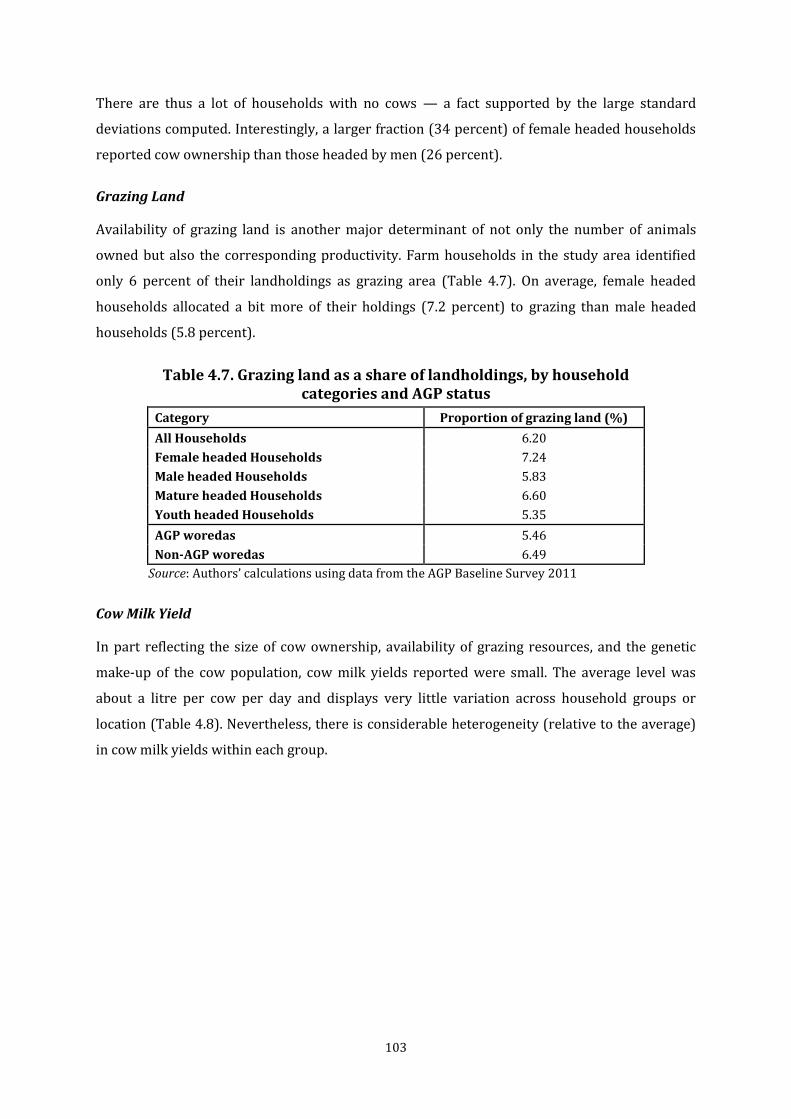
103
There are thus a lot of households with no cows — a fact supported by the large standard
deviations computed. Interestingly, a larger fraction (34 percent) of female headed households
reported cow ownership than those headed by men (26 percent).
Grazing Land
Availability of grazing land is another major determinant of not only the number of animals
owned but also the corresponding productivity. Farm households in the study area identified
only 6 percent of their landholdings as grazing area (Table 4.7). On average, female headed
households allocated a bit more of their holdings (7.2 percent) to grazing than male headed
households (5.8 percent).
Table 4.7. Grazing land as a share of landholdings, by household categories and AGP status
Category Proportion of grazing land (%)
All Households 6.20
Female headed Households 7.24
Male headed Households 5.83
Mature headed Households 6.60
Youth headed Households 5.35
AGP woredas 5.46
Non-AGP woredas 6.49
Source: Authors’ calculations using data from the AGP Baseline Survey 2011
Cow Milk Yield
In part reflecting the size of cow ownership, availability of grazing resources, and the genetic
make-up of the cow population, cow milk yields reported were small. The average level was
about a litre per cow per day and displays very little variation across household groups or
location (Table 4.8). Nevertheless, there is considerable heterogeneity (relative to the average)
in cow milk yields within each group.

104
Table 4.8. Milk yield in litre per cow per day, by AGP status
and household heads’ characteristics
Group Category
Milk Yield (litres/cow/day)
Mean SD
National
All Households 0.95 0.70
Female headed Households 1.04 0.75
Male headed Households 0.92 0.68
Mature headed Households 0.93 0.72
Youth headed Households 1.00 0.67
AGP woredas 0.93 0.73
Non-AGP woredas 0.96 0.69
Source: Authors’ calculations using data from the AGP Baseline Survey 2011. Notes: ‘SD’ stands for ‘Standard Deviation’.

105
4.4. Summary
This chapter focuses on aspects of crop and livestock productivity of households in the study
area. Accordingly, summaries of the findings on output levels, yields, and labour productivity
estimates for both crop production and livestock production are provided. Due emphasis is
attached to yield of major crop classifications. In order to capture the output and yield
estimates, crops are categorized into fifteen groups — Teff, Barley, Wheat, Maize, Sorghum,
Other Cereals, (which at some points are discussed in group as cereals), Pulses, Oilseeds,
Vegetables, Fruits, Root Crops, Coffee, Chat, Enset, Others.
In terms of area cultivated, the first striking feature is the predominance of cereals which
accounted for 66 percent of total acreage. Among cereals, teff (16.1 percent) recorded the
largest share of cultivated area, followed by maize (15.2 percent), and wheat (11.5 percent).
Regarding the acreage shares across AGP status groupings, on average, AGP woredas had larger
acreage shares going to teff, sorghum, and oil seeds. In contrast, non-AGP woredas recorded
greater shares for barley, pulses, and fruits. Although maize and wheat respectively took second
and third places in terms of acreage, they ranked first and second in output with a share of 30
percent and 17 percent respectively. Teff took the third spot with a share of 13 percent.
Estimates of output at the household level reveal that on average these outputs were not very
high during the Meher season covered. For the study area as a whole, they range from 1.3
quintals for coffee through to 5.8 quintals for maize. The median, on the other hand, is 2
quintals, implying that half of these households produced less than 2 quintals. The comparison
between AGP groups show that, among the crops considered, average household output was
higher in AGP woredas relative to non-AGP woredas for teff, wheat, maize, sorghum, pulses, oil
seeds, and chat, while average output was greater in non-AGP woredas for the other crops.
Moreover, the only statistically significant differences between households in AGP and non-AGP
woredas were observed for sorghum, pulses, and oilseeds. To complement on the perspective
provided by average output levels, average plot sizes are also computed. The findings indicate
that on average a household operated plots measuring a third of a hectare. Although the land
sizes allocated to sorghum and oilseeds were the two highest, there was no significant
difference on average plot size allotted to annual crops. When plot sizes are viewed across
gender of household heads, the findings confirm that male headed and mature headed
households had slightly bigger plots compared to those of their respective counterparts.
Average yields for each crop classification are subsequently considered. Among cereals, maize

106
turned out to have the highest yields (17.2 quintals per hectare), while teff had the lowest (9.4
quintals per hectare). This ranking held across household groups and locations. A striking
difference has been observed across mean and median estimates, however. For instance, the
mean teff yield of 9.4 quintals per hectare is matched with a median of 6.7 quintals per hectare.
In other words, half of the teff producers could only achieve teff yields of less than 6.7 quintals
per hectare. Statistically significant differences in mean yields were registered across household
types. Female headed households achieved lower yields in teff, barley, maize, and root crop
production. These differences amounted to 1-2 quintals per hectare. However, there is no
significant difference recorded between AGP and non-AGP woredas.
Labour productivity is generally characterized in terms of a ratio of the amount of output
produced to the associated amount of labour used. To do so, output per unit of labour (in adult
equivalent labour (or work day) is estimated. For all farm households, mean levels of labour
productivity measured ranged from 9.7 kg for sorghum to 14 kg for barley. Labour productivity
was similar for male and female headed households, with only a labour productivity difference
for oilseeds — female headed households produced 1 kg less oilseeds per labour day than male
headed households — and for maize — female headed households produced 1.5 kg more maize
per labour day than male headed households. However, young headed households had slightly
higher labour productivity levels compared to mature headed households for almost all crops,
with the highest difference recorded for teff (2.2 kg). Similarly, AGP woredas had slightly higher
labour productivity levels than non-AGP woredas, with the highest difference shown for
sorghum (2.8kg).
Livestock productivity indices are intrinsically more complex with corresponding data
challenges. But some indicative measures are computed. On average, cattle-owning farm
households in the study area owned 3.6 heads of cattle. Male headed households, mature
headed households, and households in AGP woredas owned more cattle than their counterparts.
Availability of grazing land is another major determinant of not only the number of animals
owned but also the corresponding productivity. Farm households in the study area identified
only 6 percent of their landholdings as grazing area. On average, female headed households
allocated a bit more of their holdings (7.2 percent) to grazing than male headed households (5.8
percent). The average milk yield was about a litre per cow per day and displays very little
variation across household groups or location. Nevertheless, there is considerable
heterogeneity (relative to the average) in cow milk yields within each group.

107
Chapter 5: Input use in crop production
In this chapter we describe the types of inputs used in crop production along with the
corresponding magnitudes and intensity of applications. We start with land. We describe the
number, characteristics, and size of plots cultivated as well as average acreage by households.
Second, we provide descriptive statistics for labour. Application rates of modern inputs
including fertilizer, improved seeds, soil conservation methods, and extension services will be
discussed in the third subsection. The subsection will also discuss fertilizer application trends in
the recent past and problems associated with adoption and/or application rates of fertilizer and
other modern inputs. The final section summarizes.
5.1. Land
Land Use
In this subsection we first describe the number, size, and other characteristics of plots cultivated
during the 2010/11 Meher season. Then we consider household and crop specific average
cultivated area.
Number and Characteristics of Plots Cultivated
A total of 45.2 million plots of varies sizes were cultivated with temporary (annual) and
permanent (perennial) crops during the Meher season within which the survey was conducted.
Out of this total, 79.2 percent were fully and 2.3 percent were partially cultivated with
temporary crops. About 18.5 percent were under permanent crops.
On average, a household in the study area operated 5.1 plots, the average size of a plot being
0.25 hectares (Tables 5.1-5.2). Slightly more than half of the households operated 4 or less plots.
The most common number of plots was 3; 16 percent of all households reported to cultivate 3
plots. Overall, male headed households farmed larger total cultivated area (1.44 ha) and had
slightly higher number of plots (5) than female headed households (1.06 ha and 4 plots,
respectively) (Table 5.1 and 5.3). While 60.9 percent of female headed households cultivated 4
or fewer plots, the corresponding figure for male headed households was only 43.6 percent.

108
Table 5.1. Average number of plots operated, by household categories, AGP status, and region (100% = all households in that category)
Groups Category Households with the given number of plots (%)
Total number of
plots operated
1 2 3 4 5 6 7 8 9 and above
Mean SD
National
All HHs 6.61 11.41 15.82 14.89 13.80 11.1 8.99 5.92 11.48 5.09 2.94
Female HHHs 11.43 16.98 17.98 14.53 13.21 8.48 7.51 4.06 5.82 4.22 2.56
Male HHHs 4.56 9.05 14.9 15.04 14.05 12.21 9.62 6.71 13.86 5.45 3.01
Mature HHHs 5.84 10.06 15.46 15.65 14.32 10.68 8.54 6.22 13.24 5.28 3.06
Youth HHHs 7.89 13.68 16.42 13.61 12.92 11.80 9.76 5.43 8.50 4.76 2.69
AGP woredas
All HHs 6.60 9.87 15.10 15.14 15.09 10.46 8.18 5.91 13.64 5.23 2.97
Female HHHs 12.64 15.71 17.09 14.76 15.18 7.62 6.85 2.81 7.34 4.24 2.61
Male HHHs 4.09 7.44 14.25 15.30 15.05 11.65 8.74 7.20 16.3 5.65 3.01
Mature HHHs 5.79 9.47 14.95 14.70 14.87 9.64 9.08 6.31 15.19 5.42 3.10
Youth HHHs 8.03 10.58 15.33 15.91 15.47 11.90 6.61 5.19 10.98 4.90 2.70
Non-AGP woredas
All HHs 6.61 11.89 16.04 14.81 13.40 11.3 9.25 5.93 10.79 5.04 2.93
Female HHHs 11.07 17.36 18.25 14.46 12.61 8.74 7.72 4.44 5.35 4.21 2.54
Male HHHs 4.71 9.55 15.10 14.96 13.73 12.39 9.90 6.56 13.11 5.40 3.01
Mature HHHs 5.86 10.25 15.62 15.94 14.14 11.01 8.37 6.19 12.62 5.23 3.05
Youth HHHs 7.85 14.6 16.75 12.93 12.17 11.77 10.70 5.50 7.73 4.72 2.68
Source: Authors’ calculations using data from the AGP Baseline Survey 2011. Notes: ‘HHHs’ and ‘HHs’ stand respectively for ‘Headed Households’ and ‘Households’. The proportions in Column 3–11 do not exactly sum up to slightly less than 100 because of rounding.
A larger proportion of households with young heads operated fewer plots relative to those with
mature heads. Moreover, average plot sizes cultivated by households with young heads were
relatively smaller. About 52 and 47 percent of households headed with young and mature heads
operated 4 or fewer plots, respectively.
The average number of plots cultivated by households in non-AGP woredas is almost the same
as the average in AGP woredas. However, AGP households cultivate slightly larger plots,
resulting in slightly larger average cultivated area in AGP woredas. The pattern and difference in
the number of plots operated by young and mature observed in the aggregated sample also
holds in both AGP and non-AGP woredas. Similarly, as observed in the case of all households,
male headed ones cultivate more plots in both AGP and non-AGP woredas. However, the
difference in the average number of plots cultivated by male and female headed households is
larger in AGP woredas.

109
According to respondents, a plot on average was located at about 15 minutes walking distance
from farmers’ residences. Plots cultivated by households headed by male and young are farther
away from their homes relative to those operated by female and mature headed households.
The last observation also holds in both AGP and non-AGP woredas. Nevertheless, differences in
the distance of plots from the homestead across categories were not large (Table 5.2).
Table 5.2. Average household plot area and characteristics of plots, by household categories and AGP status
Group Category Average plot size
(ha)
Plot distance from
homestead (minutes)
Soil quality (%)________ Plot slope (%)_
Fertile Moderately
fertile Poorly fertile
Flat Steep
National
All HHs 0.26 15.3 57.6 32.2 10.2 68.0 29.0
Female HHHs 0.25 12.9 57.1 32.4 10.5 68.3 29.9
Male HHHS 0.26 16.0 59.1 31.5 9.4 69.6 29.0
Mature HHHs 0.27 14.8 57.6 32.7 9.6 68.3 30.1
Youth HHHs 0.25 16.1 57.6 31.9 10.5 68.8 29.5
AGP woredas
All HHs 0.28 16.0 59.9 31.9 8.1 66.8 31.4
Female HHHs 0.26 14.7 59.2 32.5 8.3 73.7 25.1
Male HHHS 0.29 16.4 62.2 30.2 7.7 76.7 22.1
Mature HHHs 0.29 15.3 60.3 31.9 7.9 74.2 24.6
Youth HHHs 0.27 17.5 59.8 32.0 8.3 74.5 24.3
Non-AGP woredas
All HHs 0.25 15.0 56.9 32.3 10.9 74.4 24.4
Female HHHs 0.25 12.3 56.5 32.4 11.2 66.6 31.4
Male HHHS 0.26 15.9 58.2 31.9 9.9 67.4 31.1
Mature HHHs 0.26 14.7 56.8 33.0 10.0 66.5 31.7
Youth HHHs 0.24 15.7 56.9 31.9 11.2 66.9 31.2
Source: Authors’ calculations using data from the AGP Baseline Survey 2011. Notes: ‘HHHs’ and ‘HHs’ stand respectively for ‘Headed Household’ and ‘Households’.
Farmers were asked to characterize their plots as fertile, moderately fertile, and poorly fertile.
About 58 percent of the plots cultivated during Meher 2010/11 were categorized as fertile, 32
percent moderately fertile, and the remaining 10 percent poorly fertile (Table 5.2). Although the
proportions marginally vary, the rank order of the three fertility classes remains the same
across gender, ages, and woreda categories. Farmers were also asked whether they consider
their plots as flat, which is easy to cultivate, steep, or very steep. About 68 percent of the plots
were flat, 29 percent steep, and the remaining 3 percent were very steep12. Again, the relative
share of the three qualitative slope measures remains more or less the same across the different
categories and woredas with only slight differences in the proportions. Among the differences
worth mentioning are: a relatively larger proportion of plots in non-AGP woredas are flat and a
slightly larger proportion in AGP woredas are steep. 12 In Table 5.2, the share of the ‘very steep’ category can be obtained as 100 less the sum of the percentage share of the ‘flat’ and ‘steep’ categories.

110
Area Cultivated
On average, households used 1.32 hectares of land to grow temporary and permanent crops
during the 2010/11 Meher season in the study area, with male and mature headed households
cultivating larger area than their counterparts (Table 5.3).13 The mean area cultivated in non-
AGP woredas was slightly smaller relative to those in AGP woredas. However, there is a wide
variation in cultivated area across households with male and female heads in non-AGP and AGP
woredas. While an average male headed household in non-AGP woredas cultivated 30 percent
more land relative to those with female heads, this number was 51 percent in AGP woredas. The
average area cultivated by female headed households in non-AGP woredas is the smallest
among male and female headed households in the two woreda categories. Mature headed
households cultivated 19 percent larger area relative to the average by households with young
heads. This pattern is somehow similar among households in both non-AGP and AGP woredas.
Table 5.3. Average household cultivated area (ha), by household categories, AGP status, and region
Groups Category All Sample Without Western and North western Tigray
National
All HHs 1.32 1.31
Male HHHs 1.44 1.42
Female- HHHs 1.06 1.05
Mature HHHs 1.41 1.39
Youth HHHs 1.18 1.17
AGP woredas
All HHs 1.47 1.42
Male HHHs 1.63 1.58
Female- HHHs 1.08 1.06
Mature HHHs 1.55 1.51
Youth HHHs 1.33 1.29
Non-AGP woredas
All HHs 1.28 1.27
Male HHHs 1.37 1.37
Female HHHs 1.05 1.05
Mature HHHs 1.36 1.36
Youth HHHs 1.13 1.14
Regions
Tigray 1.66 1.13 Amhara 1.47 1.47 Oromiya 1.39 1.39 SNNP 1.01 1.01
Source: Authors’ calculations using data from the AGP Baseline Survey 2011. Notes: ‘HHHs’ and ‘HHs’ stand respectively for ‘Headed Households’ and ‘Households’.
13 The last column in Table 5.3 is added to clarify why Tigray came out as the region with the highest mean area cultivated among the four regions. The table shows that the inclusion of the relatively land abundant Western Tigray and North Western Tigray zones explains the outcome. Given the relative abundance of land, households in these zones cultivate some of the largest plots of land in the country. Excluding households in these zones reduces the area cultivated by an average household in the aggregated sample to 1.13 hectares. This is a reduction by only 1.1 percent from the average including those zones. However, average cultivated area in Tigray region without the Western and North Western Tifray zones is 1.13 hectares, which is about 43 percent lower than the average computed for households in Tirgray with these zones included (1.66 ha) — an inclusion which made the region with the highest mean area cultivated among the four regions.

111
The distribution of cultivated acreage provides additional information. Figure 5.1 below
summarizes acreage and percentiles of households with corresponding cultivated area. The
average area of 1.32 hectares hides the important fact that a large majority of the households
cultivate very small areas. In the aggregated sample, 50 percent of the households cultivated
less than 0.94 hectares. More revealing, however, is the difference in average area that the
upper 50 percent of households are cultivating compared to the lower half of households:
average cultivated area is 2.2 hectares for the former compared to 0.48 ha for the latter; or the
upper 50 percent of households are cultivating an area that is 4.6 times larger than that of the
lower half of households.. Similarly, about 5 percent of the households cultivate about one-
eighth of a hectare or smaller and about 10 percent cultivate one-fifth of a hectare or smaller.
Only 42 percent of the households cultivate an area that is equal to or larger than the average
area of 1.14 hectares.
Figure 5.1. Distribution of household’s cultivated area
01
23
45
67
89
1011
1213
Per
cent
Mean-1SD +1SD+2SD+3SD
0 1 2 3 4 5 6 7 8cultivated_area_by_hh_ha
Source: Authors’ calculations using data from the AGP Baseline Survey 2011. Notes: ‘SD’, ‘hh’ and ‘ha’ represent ‘Standard Deviation’, ‘Household’, and ‘hectare’, respectively.
In Table 5.4 we summarize average area used to cultivate teff, barley, wheat, maize, and
sorghum, pulses, oil seeds, vegetables, root crops, fruits, enset, chat, and coffee. Area allocated to
grow cereals accounted for the largest proportion of total area. In addition, for each of the five
cereals more land was used than for most other crop categories. Households that grow sorghum
allocated the largest area to sorghum relative to all other crops or cop categories. Oilseeds and
teff share the second place in crop acreage. . Wheat, maize, and barely, in that order, get the next
three rankings in crop acreage. The average cultivated area under each crop/crop category
varied little ranging from 0.49 hectares in sorghum to 0.20 hectares in chat.

112
The importance of crops in area for male headed households is mostly similar to that for all
households. In contrast, the area allocated by households with female heads differs more. Unlike
an average household in the aggregated sample, households with female heads allocated the
largest area for fruits, oilseeds, and sorghum respectively while barley and teff are equally
important at 4th place. Given that households with male heads on average cultivate larger area
they allocate more land for most crops. The exceptions to this are barley, enset, and chat, in
which the averages for both genders were equal, and root crops and fruits in which households
with female heads allocated 39 and 69 percent more land, respectively. For households with
mature heads the importance of the crops in terms of area was similar to that for an average
household with the exception that that sorghum and teff share the first place in acreage, and
that coffee is more important than fruits. For households with young heads, fruits are more
important than teff; as such, fruits are the third most important crop in terms of area cultivated.
Again, given the larger average area households with mature heads cultivate they allocate more
land for teff, barley, wheat, maize, pulses, vegetables, root crops, enset, chat and coffee.
However, these differences were small when comparing them with corresponding differences
for households with male and female heads.

113
Table 5.4. Average area cultivated by crop, by household categories, AGP status and crop classification
Group Category Statistic Teff Barely Wheat Maize Sorghum Pulses Oil
Seeds Vege
tables Root
Crops Fruit Crops
Enset Chat Coffee
National
All HHs
Mean 0.46 0.38 0.41 0.39 0.49 0.34 0.46 0.23 0.25 0.34 0.26 0.20 0.33
Rank 2 5 3 4 1 6 2 10 9 6 8 11 7
SD 0.48 0.51 0.47 0.58 0.49 0.48 0.56 0.73 0.63 0.82 0.39 0.40 0.53
Female HHHs
Mean 0.38 0.38 0.37 0.32 0.40 0.31 0.44 0.18 0.32 0.49 0.26 0.21 0.28
SD 0.31 0.46 0.35 0.46 0.40 0.53 0.42 0.56 0.80 1.15 0.39 0.40 0.42
Male HHHs
Mean 0.49 0.38 0.43 0.42 0.53 0.35 0.47 0.26 0.23 0.29 0.26 0.20 0.35
SD 0.52 0.52 0.50 0.63 0.52 0.46 0.59 0.78 0.55 0.65 0.40 0.40 0.56
Mature HHHs
Mean 0.49 0.39 0.43 0.41 0.49 0.36 0.44 0.25 0.27 0.30 0.27 0.21 0.35
SD 0.52 0.46 0.51 0.62 0.49 0.50 0.51 0.79 0.68 0.67 0.40 0.42 0.58
Youth- HHHs
Mean 0.41 0.36 0.38 0.35 0.50 0.30 0.49 0.20 0.23 0.43 0.25 0.19 0.30
SD 0.39 0.58 0.38 0.51 0.50 0.45 0.63 0.59 0.53 1.06 0.38 0.34 0.39
AGP woredas
All HHs
Mean 0.52 0.34 0.43 0.34 0.68 0.37 0.69 0.20 0.25 0.33 0.25 0.29 0.35
Ranks 3 7 4 7 2 5 1 11 10 8 10 9 6
SD 0.56 0.34 0.49 0.47 0.64 0.48 0.77 0.63 0.63 0.95 0.41 0.58 0.77
Female HHHs
Mean 0.43 0.32 0.42 0.27 0.53 0.34 0.59 0.17 0.19 0.36 0.24 0.28 0.28
SD 0.39 0.28 0.42 0.39 0.45 0.43 0.64 0.55 0.33 1.05 0.37 0.61 0.62
Male HHHs
Mean 0.55 0.34 0.43 0.36 0.73 0.38 0.72 0.21 0.27 0.32 0.26 0.29 0.38
SD 0.60 0.36 0.51 0.50 0.68 0.50 0.80 0.66 0.70 0.91 0.42 0.57 0.82
Mature HHHs
Mean 0.55 0.35 0.45 0.35 0.70 0.40 0.69 0.23 0.24 0.32 0.26 0.29 0.38
SD 0.61 0.35 0.52 0.51 0.66 0.51 0.80 0.75 0.62 0.94 0.42 0.61 0.86
Youth HHHs
Mean 0.46 0.31 0.39 0.32 0.66 0.32 0.70 0.15 0.28 0.36 0.24 0.28 0.30
SD 0.45 0.32 0.43 0.39 0.61 0.43 0.72 0.36 0.65 0.95 0.40 0.52 0.53
Non-AGP woredas
All HHs Mean 0.44 0.39 0.41 0.41 0.42 0.33 0.37 0.25 0.25 0.35 0.26 0.17 0.33
SD 0.44 0.54 0.46 0.62 0.41 0.48 0.43 0.77 0.63 0.78 0.39 0.29 0.46
Female HHHs
Mean 0.36 0.39 0.35 0.34 0.36 0.30 0.39 0.18 0.35 0.53 0.26 0.19 0.28
SD 0.26 0.49 0.32 0.48 0.37 0.55 0.29 0.57 0.87 1.18 0.40 0.26 0.36
Male HHHs
Mean 0.46 0.39 0.42 0.44 0.45 0.34 0.37 0.28 0.22 0.28 0.26 0.16 0.35
SD 0.48 0.56 0.50 0.66 0.42 0.45 0.46 0.85 0.50 0.53 0.39 0.30 0.49
Mature HHHs
Mean 0.46 0.40 0.42 0.44 0.42 0.35 0.34 0.26 0.28 0.29 0.27 0.18 0.34
SD 0.47 0.49 0.51 0.66 0.40 0.49 0.29 0.81 0.69 0.55 0.40 0.32 0.51
Youth HHHs
Mean 0.39 0.37 0.38 0.36 0.43 0.30 0.42 0.23 0.22 0.46 0.25 0.14 0.30
SD 0.36 0.62 0.36 0.54 0.43 0.46 0.58 0.70 0.48 1.10 0.38 0.21 0.36
Source: Authors’ calculations using data from the AGP Baseline Survey 2011. Notes: ‘HHHs’ and ‘HHs’ stands respectively for ‘Headed Households’ and ‘Households’. ‘SD’ stands for ‘Standard Deviation’.
The ranking of crop importance in terms of area cultivated for households in AGP woredas
shows several differences compared the ranking for the households in the aggregated sample. A
remarkable difference is that households in AGP woredas allocated the biggest share of land to
oil seeds and a greater share of land to coffee than to maize and barley — maize and barley
dropped as such to the seventh ranking, compared to the 4th and 5th place in the aggregated
sample. In addition, households in AGP woredas also allocated a larger share of land to chat
cultivation; in fact, in terms of allocated land, chat was more important than enset, root crops

114
and vegetables. In terms of average cultivated area for each crop, households in AGP woredas
allocated 70, 62, 86, 18, and 6 percent more area to grow chat, sorghum, oilseeds, teff, and
coffee, respectively, compared to households in non-AGP woredas. By contrast households in
non-AGP woredas allocated 15 percent larger area for barley, and 21, 25, 6, and 4 percent larger
area to grow maize, vegetables, fruits, and enset, respectively. There was no difference in root
crops area.
Land Tenure and Registration
The survey included questions regarding sources of cultivated plots and whether or not the plot
was registered. The findings are summarized in Table 5.5.
The large majority of the plots that households cultivated in the Meher 2010/11 season were
inherited from relatives (48 percent). This is 40 percent higher than the proportion of plots that
were directly allocated by the government to their current tenants, which is 35 percent. The
proportion of plots owned by other households but cultivated through some arrangement is
about 16 percent of the total. This is largely composed of share-cropped (8 percent) and rented-
in (6 percent) land. It is interesting to note that over 0.6 million plots are borrowed/rented for
free. The vast majority of the plots (82 percent) that were cultivated by the households were
registered. By registering a plot with the local authority households get certificates
acknowledging their user rights.
Households with female heads acquired a larger proportion of plots directly from the
government (43 percent) than households with male heads (31 percent). Given the fact that
farmers associations are required to allocate land without gender discrimination the difference
in the proportion allocated to households with female and male heads is considerably wide. For
both male and female headed households the proportion of plots inherited was 48 percent. A
slightly larger proportion of cultivated by female headed households are registered.
The proportion of plots that are allocated by the government increases with age, indicating that
younger household heads have to find land through other means than government allocation.
Moreover, the proportion of plots households acquired through inheritance declines with the age
of the head. Thus, for households with younger heads inheritance is a more important means of
land acquisition. The ratio of proportion inherited to proportion allocated is roughly 3.1 for
households with young heads. It is also interesting to note that households with younger heads use
more plots from others through the means of renting and share-cropping relative to households
with older heads. Mature headed households have a larger proportion of plots registered than

115
young headed households.
Table 5.5. Sources of user rights of cultivated land (%)
Groups Category
Own plots Others' plots
Proportion registered Allocated Inherited Mortgaged Rented-in
Share-cropped
Borrowed free
National
All HHs 34.2 47.9 0.3 4.2 6.3 1.9 81.9
Female HHHs 42.7 48.2 0.1 1.6 1.8 1.2 82.3
Male HHHs 31.3 47.9 0.3 5.0 7.7 2.1 81.8
Mature HHHs 43.8 41.3 0.3 3.0 4.0 2.3 85.4
Youth HHHs 14.0 61.9 0.1 6.7 11.1 0.9 74.5
Total AGP Sample
All HHs 38.2 43.2 0.6 5.2 8.0 0.6 80.9
Female HHHs 51.1 40.2 0.4 1.7 1.8 0.6 82.0
Male HHHs 34.1 44.2 0.7 6.3 10.0 0.6 82.2
Mature HHHs 49.0 37.9 0.7 3.7 4.8 0.7 85.1
Youth HHHs 14.4 55.0 0.5 8.4 15.2 0.4 76.2
Total Non-AGP Sample
All HHs 32.9 49.5 0.2 3.8 5.7 2.3 82.2
Female HHHs 40.1 50.7 0.0 1.6 1.8 1.4 83.0
Male HHHs 30.5 49.1 0.2 4.6 7.0 2.6 80.3
Mature HHHs 42.1 42.4 0.2 2.7 3.7 2.9 86.4
Youth HHHs 13.8 64.0 0.0 6.1 9.8 1.1 69.0 Source: Authors’ calculations using data from the AGP Baseline Survey 2011 Notes: ‘HHHs’ and ‘HHs’ stand respectively for ‘Headed Households’ and ‘Households’. Row percentages are not equal to 100% as some means of acquiring land are not reported.
Compared to households in non-AGP woredas, households in AGP woredas had a larger
proportion of directly allocated plots and a smaller proportion of inherited plots. Considering
the remaining source, the proportions of rented-in and share-cropped plots were about 39
percent larger in AGP households, while the proportion of freely rented plots was 3.8 times
larger in non-AGP households.
5.2. Labour use
The AGP baseline survey collected data on the number of days (as opposed to hours) spent on
performing different tasks of production. As such, any crop production activity of any length is
considered as a work day. We converted the total number of days that each household member
of a specific age and gender contributed into adult male equivalents. We summarize the
estimated average labour use per hectare in Table 5.6. It is important to note as a caveat that the
labour days reported by respondents were not necessarily equal to full working days in every
case. It is also unlikely that these days were identical across crops and/or activities. Reasonable
adjustments for these features were not possible due to lack of the requisite data. Note also that,
although the labour days are expressed on a per hectare basis only by far, the largest fraction of
crop-specific cultivated area is much less than a hectare.

116
Labour days used to grow sorghum are more than twice the one for chat, which has the second
largest number of days. While sorghum requires more care during fruition to harvest, this large
number may indicate labour use that grows proportionally faster than area. Among cereals, in
the number of adult equivalent work days, teff was second from last, next to wheat, while
considerably more labour was used per hectare of barley and maize grown. The smallest
number of family labour days was used to cultivate oilseeds.
The importance of crops in terms of number of family labour used by female headed households
is different from the aggregated sample for all crops except for oilseeds and enset. Male headed
households perform relatively similar with an average household. However, the number of
median work days used to grow each crop by female and male headed households differs from
the aggregated median. The importance of crops in terms of the number of work days is very
different between households with mature heads and households with young heads. The
importance of crops in terms of the number of work days is also very different between
households in AGP woredas and households in non-AGP woredas.
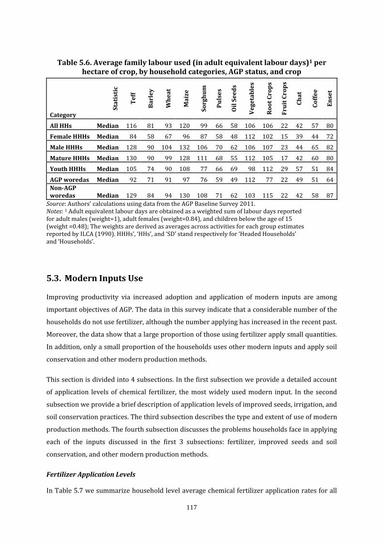
117
Table 5.6. Average family labour used (in adult equivalent labour days)1 per hectare of crop, by household categories, AGP status, and crop
Category S
tati
stic
Te
ff
Ba
rle
y
Wh
ea
t
Ma
ize
So
rgh
um
Pu
lse
s
Oil
Se
ed
s
Ve
ge
tab
les
Ro
ot
Cro
ps
Fru
it C
rop
s
Ch
at
Co
ffe
e
En
set
All HHs Median 116 81 93 120 99 66 58 106 106 22 42 57 80
Female HHHs Median 84 58 67 96 87 58 48 112 102 15 39 44 72
Male HHHs Median 128 90 104 132 106 70 62 106 107 23 44 65 82
Mature HHHs Median 130 90 99 128 111 68 55 112 105 17 42 60 80
Youth HHHs Median 105 74 90 108 77 66 69 98 112 29 57 51 84
AGP woredas Median 92 71 91 97 76 59 49 112 77 22 49 51 64
Non-AGP woredas Median 129 84 94 130 108 71 62 103 115 22 42 58 87
Source: Authors’ calculations using data from the AGP Baseline Survey 2011. Notes: 1 Adult equivalent labour days are obtained as a weighted sum of labour days reported for adult males (weight=1), adult females (weight=0.84), and children below the age of 15 (weight =0.48); The weights are derived as averages across activities for each group estimates reported by ILCA (1990). HHHs’, ‘HHs’, and ‘SD’ stand respectively for ‘Headed Households’ and ‘Households’.
5.3. Modern Inputs Use
Improving productivity via increased adoption and application of modern inputs are among
important objectives of AGP. The data in this survey indicate that a considerable number of the
households do not use fertilizer, although the number applying has increased in the recent past.
Moreover, the data show that a large proportion of those using fertilizer apply small quantities.
In addition, only a small proportion of the households uses other modern inputs and apply soil
conservation and other modern production methods.
This section is divided into 4 subsections. In the first subsection we provide a detailed account
of application levels of chemical fertilizer, the most widely used modern input. In the second
subsection we provide a brief description of application levels of improved seeds, irrigation, and
soil conservation practices. The third subsection describes the type and extent of use of modern
production methods. The fourth subsection discusses the problems households face in applying
each of the inputs discussed in the first 3 subsections: fertilizer, improved seeds and soil
conservation, and other modern production methods.
Fertilizer Application Levels
In Table 5.7 we summarize household level average chemical fertilizer application rates for all

118
households and for households that actually applied chemical fertilizer. In the aggregated
sample, 58 percent of households in the study area used chemical fertilizers during the Meher
2010/11. On average, farm households in the study area applied 27 kg of chemical fertilizer
made up of DAP and urea separately or together per plot. This pattern holds more or less across
male and female and mature and young headed households. On average, male headed
households applied 46 percent more chemical fertilizers compared to female headed
households. This gap narrows down considerably when we compare actual users only (see
below). Relative to households with young heads, those with mature heads used 10 percent
more chemical fertilizer.
Table 5.7. Proportion of chemical fertilizer users and average application rate of fertilizer on a plot of land for all farmers and users only (in kg), by household
categories and AGP status
Group Category Chemical fertilizer
users (%)
DAP-All farmers
(kg)
DAP-User farmers
Only (kg)
Urea-All farmers
(kg)
Urea-User
farmers only (kg)
DAP+Urea-All farmers
(kg)
DAP+Urea-User
farmers only (kg)
National
All HHs 57.6 17.2 33.7 9.7 28.6 27.0 49.2
Female HHHs 48.2 13.5 31.1 6.9 25.2 20.4 44.0
Male HHHs 61.7 18.8 34.5 10.9 29.7 29.7 51.0
Mature HHHs 57.7 17.7 34.6 10.2 29.5 27.9 51.0
Youth HHHs 57.4 16.3 32.1 9.0 27.0 25.4 46.3
AGP woredas
All HHs 62.3 19.3 37.0 12.7 31.8 32.0 55.0
Female HHHs 51.2 13.4 32.7 9.3 28.5 22.7 47.7
Male HHHs 67.0 19.3 38.4 14.1 32.9 33.4 57.0
Mature HHHs 62.1 17.8 37.5 13.2 32.5 31.0 55.8
Youth HHHs 62.7 17.1 36.1 12.0 30.8 29.1 52.9
Non-AGP woredas
All HHs 55.7 16.6 32.6 8.8 27.4 25.4 47.3
Female HHHs 46.9 13.5 30.6 6.0 23.6 19.5 42.6
Male HHHs 59.5 18.6 33.1 9.6 28.0 28.2 48.5
Mature HHHs 55.9 17.7 33.5 9.0 28.0 26.6 49.0
Youth HHHs 55.3 16.1 30.7 7.9 25.1 23.9 43.7
Source: Authors’ calculations using data from the AGP Baseline Survey 2011. Notes: ‘HHHs’ and ‘HHs’ stands respectively for ‘Headed Households’ and ‘Households’.
Around 12 percent more households used chemical fertilizer in AGP woredas compared to those
in non-AGP woredas. As was observed in the aggregated sample, on average male and mature
headed households applied more chemical fertilizer than female and young headed households
in both AGP and non-AGP woredas. Moreover, all subgroups of households in AGP woredas
apply more chemical fertilizer relative to their counterparts in non-AGP woredas.
Average chemical fertilizer application rates of households that actually used chemical fertilizer
is also presented in Table 5.7. The fact that only 57 percent of the households applied chemical
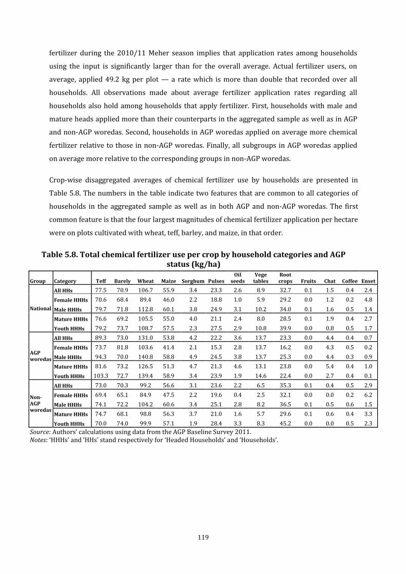
119
fertilizer during the 2010/11 Meher season implies that application rates among households
using the input is significantly larger than for the overall average. Actual fertilizer users, on
average, applied 49.2 kg per plot — a rate which is more than double that recorded over all
households. All observations made about average fertilizer application rates regarding all
households also hold among households that apply fertilizer. First, households with male and
mature heads applied more than their counterparts in the aggregated sample as well as in AGP
and non-AGP woredas. Second, households in AGP woredas applied on average more chemical
fertilizer relative to those in non-AGP woredas. Finally, all subgroups in AGP woredas applied
on average more relative to the corresponding groups in non-AGP woredas.
Crop-wise disaggregated averages of chemical fertilizer use by households are presented in
Table 5.8. The numbers in the table indicate two features that are common to all categories of
households in the aggregated sample as well as in both AGP and non-AGP woredas. The first
common feature is that the four largest magnitudes of chemical fertilizer application per hectare
were on plots cultivated with wheat, teff, barley, and maize, in that order.
Table 5.8. Total chemical fertilizer use per crop by household categories and AGP status (kg/ha)
Group Category Teff Barely Wheat Maize Sorghum Pulses Oil
seeds Vege
tables Root crops Fruits Chat Coffee Enset
National
All HHs 77.5 70.9 106.7 55.9 3.4 23.3 2.6 8.9 32.7 0.1 1.5 0.4 2.4
Female HHHs 70.6 68.4 89.4 46.0 2.2 18.8 1.0 5.9 29.2 0.0 1.2 0.2 4.8
Male HHHs 79.7 71.8 112.8 60.1 3.8 24.9 3.1 10.2 34.0 0.1 1.6 0.5 1.4
Mature HHHs 76.6 69.2 105.5 55.0 4.0 21.1 2.4 8.0 28.5 0.1 1.9 0.4 2.7
Youth HHHs 79.2 73.7 108.7 57.5 2.3 27.5 2.9 10.8 39.9 0.0 0.8 0.5 1.7
AGP woredas
All HHs 89.3 73.0 131.0 53.8 4.2 22.2 3.6 13.7 23.3 0.0 4.4 0.4 0.7
Female HHHs 73.7 81.8 103.6 41.4 2.1 15.3 2.8 13.7 16.2 0.0 4.3 0.5 0.2
Male HHHs 94.3 70.0 140.8 58.8 4.9 24.5 3.8 13.7 25.3 0.0 4.4 0.3 0.9
Mature HHHs 81.6 73.2 126.5 51.3 4.7 21.3 4.6 13.1 23.8 0.0 5.4 0.4 1.0
Youth HHHs 103.3 72.7 139.4 58.9 3.4 23.9 1.9 14.6 22.4 0.0 2.7 0.4 0.1
Non-AGP woredas
All HHs 73.0 70.3 99.2 56.6 3.1 23.6 2.2 6.5 35.3 0.1 0.4 0.5 2.9
Female HHHs 69.4 65.1 84.9 47.5 2.2 19.6 0.4 2.5 32.1 0.0 0.0 0.2 6.2
Male HHHs 74.1 72.2 104.2 60.6 3.4 25.1 2.8 8.2 36.5 0.1 0.5 0.6 1.5
Mature HHHs 74.7 68.1 98.8 56.3 3.7 21.0 1.6 5.7 29.6 0.1 0.6 0.4 3.3
Youth HHHs 70.0 74.0 99.9 57.1 1.9 28.4 3.3 8.3 45.2 0.0 0.0 0.5 2.3
Source: Authors’ calculations using data from the AGP Baseline Survey 2011. Notes: ‘HHHs’ and ‘HHs’ stand respectively for ‘Headed Households’ and ‘Households’.

120
The survey also included questions on households’ use of organic fertilizer. Although about 57
percent of the households applied chemical fertilizer, a large majority (98 percent) applied
manure in their fields. It is also interesting to note that more than 90 percent of the households
applied manure to more than one-half of their fields. Out of the total plots cultivated in the
2010/11 main agricultural season more than 86 percent were applied with manure. Moreover,
about 12 percent of the households applied compost on their fields. Assuming chemical
fertilizers, manure, and compost are more or less substitutes, about 98.5 of the households used
some kind of fertilizer. Moreover, the proportion of the households that applied a combination
of these fertilizers is larger relative to those that applied only one type. The proportion of
households that applied only chemical fertilizers was small at 0.4 percent. By contrast 33 and 8
percent of the households applied only manure or compost, respectively. Moreover, 41.6
percent of the households applied chemical fertilizer and manure, while about 15 percent
applied all three types.
Average crop level per hectare fertilizer application rates of households in the different
categories and woredas that use chemical fertilizers are summarized in Table 5.9. As expected,
application rates are significantly higher when the computation is confined to users alone.
Nevertheless, note that the large increase for some of the crops is largely due to the small
number of users in the sub-sample. This is particularly true for non-cereal crops. For instance,
only 2 fruit producers reported chemical fertilizer use. The analogous number for coffee, chat,
and enset producers are 19, 35, and 37, respectively. The number of adopters was so small that
these crops were dropped from Table 5.9. The only cereal with a relatively small fertilizer-using
sub-sample is sorghum with 247 households.
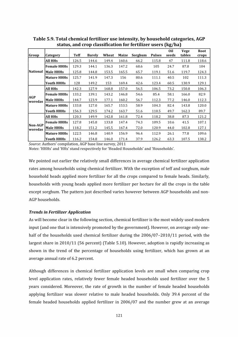
121
Table 5.9. Total chemical fertilizer use intensity, by household categories, AGP status, and crop classification for fertilizer users (kg/ha)
Group Category Teff Barely Wheat Maize Sorghum Pulses Oil
seeds Vege
tables Root crops
National
All HHs 126.5 144.6 149.4 160.6 66.2 115.8 47 111.8 118.6
Female HHHs 129.3 144.1 136.3 147.2 68.6 105 24.7 87.8 104
Male HHHs 125.8 144.8 153.5 165.5 65.7 119.1 51.6 119.7 124.3
Mature HHHs 125.7 141.9 147.3 156 80.6 111.1 40.5 102 111.3
Youth HHHs 128 149.2 153 169.4 42.6 123.4 60.5 130.9 129.1
AGP woredas
All HHs 142.3 127.9 168.8 157.0 56.5 106.5 73.2 150.8 106.3
Female HHHs 133.2 139.1 143.2 146.8 54.6 85.4 58.1 166.0 82.9
Male HHHs 144.7 123.9 177.1 160.2 56.7 112.3 77.2 146.0 112.3
Mature HHHs 133.8 127.0 165.7 153.5 58.9 104.3 82.4 143.8 120.0
Youth HHHs 156.3 129.5 174.2 163.7 51.6 110.5 49.7 162.3 89.7
Non-AGP woredas
All HHs 120.3 149.9 142.8 161.8 72.4 118.2 38.8 87.3 121.2
Female HHHs 127.8 145.8 133.8 147.4 74.3 109.5 10.6 41.5 107.1
Male HHHs 118.2 151.2 145.5 167.4 72.0 120.9 44.0 102.8 127.1
Mature HHHs 122.5 146.8 140.9 156.9 96.4 112.9 26.1 77.8 109.6
Youth HHHs 116.2 154.8 146.0 171.4 37.9 126.2 63.3 107.5 138.2
Source: Authors’ compilation, AGP base line survey, 2011 Notes: ‘HHHs’ and ‘HHs’ stand respectively for ‘Headed Households’ and ‘Households’.
We pointed out earlier the relatively small differences in average chemical fertilizer application
rates among households using chemical fertilizer. With the exception of teff and sorghum, male
household heads applied more fertilizer for all the crops compared to female heads. Similarly,
households with young heads applied more fertilizer per hectare for all the crops in the table
except sorghum. The pattern just described varies however between AGP households and non-
AGP households.
Trends in Fertilizer Application
As will become clear in the following section, chemical fertilizer is the most widely used modern
input (and one that is intensively promoted by the government). However, on average only one-
half of the households used chemical fertilizer during the 2006/07–2010/11 period, with the
largest share in 2010/11 (56 percent) (Table 5.10). However, adoption is rapidly increasing as
shown in the trend of the percentage of households using fertilizer, which has grown at an
average annual rate of 6.2 percent.
Although differences in chemical fertilizer application levels are small when comparing crop
level application rates, relatively fewer female headed households used fertilizer over the 5
years considered. Moreover, the rate of growth in the number of female headed households
applying fertilizer was slower relative to male headed households. Only 39.4 percent of the
female headed households applied fertilizer in 2006/07 and the number grew at an average

122
annual rate of 4.6 percent to get to 47 percent in 2010/11. By contrast about 46 percent of male
headed households used fertilizer in 2006/07 which grew to 59.6 percent in 2010/11 at an
average annual rate of 6.9 percent, which is 50 percent larger than the growth rate in female
headed households.
On average only 47 percent of the households with young heads applied chemical fertilizer
during the 2006/07–2010/11 period, while the average for households with mature heads was
51 percent. However, the fraction of young headed households adopting fertilizer has been
growing faster albeit from a lower base.
While about 49 percent of the households in non-AGP woredas applied chemical fertilizer
during the 5 year period, the proportion was larger in AGP woredas (53 percent). However, the
number applying fertilizer increased relatively faster over the past five years in AGP woredas by
17 percent relative to the 7 percent in non-AGP woredas. The pattern observed among male vs.
female and mature vs. young headed households in the aggregated sample also holds in both
AGP and non-AGP woredas.
Table 5.10. Trends in fertilizer application, by household categories, AGP status, and region (% of all households using chemical fertilizer)
Groups Category
Period
2006/07 2007/08 2008/09 2009/10 2010/11 Average
National
All HHs 43.8 46.8 49.9 52.5 55.8 49.8
Female-HHHs 39.4 41.3 44.1 46.4 47.1 43.7
Male HHHs 45.7 49.2 52.4 55.2 59.6 52.4
Mature HHHs 45.7 48.8 51.5 53.6 56.7 51.3
Youth HHHs 40.6 43.5 47.2 50.8 54.3 47.3
AGP woredas
All HHs 42.8 50.7 54.1 56.8 60.6 53.0
Female HHHs 41.8 43.8 45.5 47.9 50.4 45.9
Male HHHs 49.5 53.7 57.8 60.7 65.0 57.3
Mature HHHs 49.4 52.8 55.0 57.3 60.6 55.0
Youth HHHs 43.2 47.0 52.5 56.0 60.7 51.9
Non-AGP woredas
All HHs 47.2 45.6 48.6 51.2 54.4 49.4
Female HHHs 38.6 40.6 43.6 45.9 46.0 42.9
Male HHHs 44.6 47.7 50.7 53.5 57.9 50.9
Mature HHHs 44.6 47.5 50.4 52.4 55.5 50.1
Youth HHHs 39.8 42.4 45.6 49.2 52.4 45.9
Source: Authors’ calculations using data from the AGP Baseline Survey 2011. Notes: ‘HHHs’ and ‘HHs’ stand respectively for ‘Headed Households’ and ‘Households’
Application Levels of Improved Seeds, Irrigation, and Soil Conservation
Households obtain high yielding seeds either through new purchases, mostly from government
agencies, or by saving from their own output, using high yielding variety seeds bought in

123
previous seasons or years. In this survey we made an effort to measure the extent of use of both
types of seeds. Out of all plots, about 90 percent were planted with local seeds, about 1.3
percent with seeds saved from output produced by using previously bought high yielding
variety seeds, and 6.3 percent with freshly bought high yielding variety seeds (Table 5.11). The
remaining 2.1 percent were sown with a combination of the three types. While 76 percent of the
total improved seed was newly bought, the remaining 24 percent was saved from the output of
previously used improved seeds.
Although 23.5 percent of the households used improved seeds during the Meher 2010/2011
season, the amount used in the study area averaged less than a kilogram per hectare (Table
5.11). However, among users application rates of improved seeds was significantly large at
about 11.1 kg per hectare. Although the proportion of female headed households that applied
improved seeds is 8 percentage points lower compared to male headed households, application
rate was not significantly different between male and female headed households who actually
applied the input. Slightly more households with mature heads applied improved seeds.
Relative to households in AGP woredas, more households in non-AGP woredas used improved
seeds and the average application rate of improved seeds by households using the input was
larger. Both of the last observations also hold for households in all age and gender categories.
Table 5.11. Improved seed use, irrigation, and soil conservation, by household categories and AGP status (100%=all farmers)
Group Category
Improved seed users
Improved seed use – All Farmers
Improved seed use – User
Farmers Only Irrigation Soil
conservation
(%) (kg/ha) (kg/ha) (%) (%)
National
All HHs 22.5 2.1 11.1 4.2 72.4
Female HHHs 16.7 1.5 10.9 2.9 66.4
Male HHHs 24.9 2.3 11.1 4.7 75.0
Mature HHHs 22.7 2.1 10.9 4.3 73.4
Youth HHHs 22.1 2.1 11.4 4.0 70.8
AGP woredas
All HHs 22.1 2.1 10.6 7.8 71.0
Female HHHs 18.2 1.5 10.5 1.9 66.2
Male HHHs 23.7 2.4 10.6 3.6 73.2
Mature HHHs 21.8 2.1 10.1 3.1 71.0
Youth HHHs 22.6 2.1 11.2 3.0 71.1
Non-AGP woredas
All HHs 22.6 1.9 11.2 3.1 72.8
Female HHHs 16.3 1.6 11.0 6.4 66.4
Male HHHs 25.3 2.1 11.3 8.3 75.6
Mature HHHs 23.0 1.8 11.1 8.0 74.1
Youth HHHs 22.0 2.1 11.4 7.4 70.7
Source: Authors’ calculations using data from the AGP Baseline Survey 2011. Notes: ‘HHHs’ and ‘HHs’ stand respectively for ‘Headed Households’ and ‘Households’

124
In the study area only 4.2 percent of the households irrigated their plots while a significantly
large proportion (72 percent) practiced some soil conservation measures. Relative to female
headed households, the proportions of households with male heads that used irrigation and/or
soil conservation measures were larger. The same is true when comparing mature and youth
headed households, although the difference is narrower in this case. A relatively larger
proportion of AGP households irrigated their land relative to the corresponding categories of
non-AGP households. By contrast, a relatively larger proportion of all non-AGP households
applied soil conservation methods, with the exception of mature headed households in which
case the proportion was larger for AGP woredas.
Modern Production Methods
This section describes the type and use of the advice on modern production methods and inputs
that households in the study area acquire from agricultural extension agents. While application
levels of modern inputs that we described above partly measure the extent to which extension
agents were able to convince farmers into using the inputs, the description in this section shows
the efforts being made by the latter in any given year.
During the Meher season of 2010/2011 about 35 percent of the households were visited by an
extension agent at least once (Table 5.12). That more than a third of the households were
visited at least once in only one agricultural season and more than a quarter were visited more
than once is noteworthy.
A larger fraction of male headed households were visited compared to female headed
households: i.e., 46, 50, and 45 percent more households with male heads were visited at least
once in the aggregated sample, in AGP woredas, and non-AGP woredas, respectively. Relative to
households with mature heads those with young heads were also visited more in total, in AGP
woredas, and in non-AGP woredas. The percentage of households visited by extension agents is
the same for both AGP and non-AGP woredas.
Households were requested to mention the 3 important advises and assistances out of the six
listed in the questionnaire and mention others that are not on the list. Information provided on
new inputs and production methods were selected by respondents as by far the two most
important services received by visited households 35 percent and 34 percent of the households
selecting the two as most important, respectively. All household groups in all locations did the
same, though the order in which the two were selected was not always the same. Extension
agents’ help in obtaining fertilizer was the third important support identified by all groups of
households (Table 5.12).

125
Table 5.12. Main help from extension agents’ visit, by household categories and AGP status
Group Category
Proportion visited (%)
Main help from extension agent for those visited, introducing:
New inputs
New methods
New crops Fertilizer
Improved seed Credit Others
National
All HHs 35.0 34.9 34.1 6.4 12.5 6.6 0.7 4.8
Male HHHs 38.7 34.9 33.4 6.5 13.4 6.6 0.6 4.6
Female HHHs 26.5 35.1 36.3 6 9.5 6.6 1 5.6
Mature HHHs 37.1 33.4 36.3 6.8 12.8 5.9 0.8 4
Youth HHHs 31.5 37.8 29.6 5.6 12.1 8 0.6 6.3
AGP woredas
All HHs 35.0 41.7 28.4 5.5 10.6 6.7 1.0 6.0
Male HHHs 38.9 42.5 28.2 5.8 10.3 6.2 0.9 6.2
Female HHHs 26.0 39.0 29.2 4.7 11.8 8.4 1.3 5.6
Mature HHHs 35.9 40.2 30.2 6.5 10.8 5.1 0.8 6.3
Youth HHHs 33.4 44.5 25.0 3.7 10.3 9.5 1.5 5.5
Non-AGP woredas
All HHs 35.0 32.8 35.8 6.7 13.1 6.6 0.6 4.4
Male HHHs 38.7 32.5 35.1 6.8 14.4 6.7 0.6 4.1
Female HHHs 26.6 33.9 38.5 6.3 8.8 6.0 0.9 5.6
Mature HHHs 37.5 31.4 38.2 6.9 13.3 6.1 0.8 3.3
Youth HHHs 31.0 35.7 31.1 6.2 12.6 7.5 0.3 6.6
Source: Authors’ calculations using data from the AGP Baseline Survey 2011. Notes: ‘HHHs’ and ‘HHs’ stand respectively for ‘Headed Households’ and ‘Households’.
5.4. Factors contributing to low levels of use of modern inputs and
production methods
Adoption of modern inputs requires timely and sufficient availability of these inputs. It may also
require access to credit, in addition to the information households obtain on the inputs and
production methods. This section looks at some of such and related challenges faced by
households in the study area.
Households were asked to name the three most important problems they face in accessing
fertilizer whether or not they applied fertilizer. While 87.6 percent indicated they faced at least
one problem, 12.4 percent indicated they did not have a problem or the question was not
relevant for them. A summary of the problems indicated as important by the households
surveyed are summarized in Table 5.13.

126
Table 5.13. Constraints to fertilizer adoption — proportion of households reporting as most important constraint to adoption (%), by household categories
and AGP status
Groups Category Shortage of supply
Arrived late
High price
Lack of credit
Others No problem/ not relevant
National
All HHs 20.4 12.0 35.9 14.5 4.7 12.4
Female HHHs 19.3 10.6 35.3 14.7 5.9 14.2
Male HHHs 20.9 12.7 36.2 14.4 4.2 11.6
Mature HHHs 20.9 11.9 36.3 14.0 4.5 12.4
Youth HHHs 19.6 12.3 35.1 15.4 5.0 12.5
AGP woredas
All HHs 16.5 11.9 40.8 12.2 14.0 4.7
Female HHHs 16.1 11.6 38.6 12.5 15.4 5.9
Male HHHs 16.7 12.0 41.7 12.1 13.4 4.2
Mature HHHs 16.3 12.2 41.4 11.3 14.1 4.8
Youth HHHs 17.0 11.3 39.7 13.8 13.8 4.4
Non-AGP woredas
All HHs 21.6 12.1 34.4 15.2 12.0 4.7
Female HHHs 20.3 10.2 34.3 15.4 13.9 5.9
Male HHHs 22.2 12.9 34.5 15.1 11.1 4.2
Mature HHHs 22.4 11.8 34.8 14.8 11.8 4.4
Youth HHHs 20.4 12.6 33.8 15.9 12.2 5.2
Source: Authors’ calculations using data from the AGP Baseline Survey 2011. Notes: ‘HHHs’ and ‘HHs’ stand respectively for ‘Headed Households’ and ‘Households’
The problem that is cited as important by most households (36 percent) is the high price of
fertilizer. It was also second in importance among households that selected another problem as
first. The second important factor that contributed to low levels of adoption or application of
fertilizer was shortage of supply. The first and second problems were also selected by most
households in all categories in the aggregated sample, in AGP woredas, and in non-AGP
woredas. The third and fourth important factors were unavailability of credit and untimely
arrival of fertilizer supply.
There are significant differences in the factors cited as important across AGP and non-AGP
woredas. Relative to AGP households, a larger fraction of non-AGP households deemed shortage
of supply and lack of credit as more important constraints. In contrast, a considerably large
proportion of households in AGP woredas considered high fertilizer price as the most important
limitation.
The survey questionnaire also included questions on timely availability and/or use of inputs as
well as credit. In Table 5.14 below we summarize the inputs that were made available before
the start of the season.

127
Table 5.14. Availability of modern inputs — proportion of households reporting availability in time (%), by household categories and AGP status (100% = all
households)
Group Category Input available before the start of the main planting season
Fertilizer Local seed Improved seed Other inputs
National
All HHs 52.6 72.1 34.8 46.5
Male HHHs 49.6 72.5 32.0 43.0
Female HHHs 53.9 71.9 36.0 47.9
Mature HHHs 51.4 71.5 33.7 46.3
Youth HHHs 54.6 73.0 36.7 46.8
AGP woredas
All HHs 56.5 58.9 29.9 49.7
Male HHHs 58.6 76.0 37.4 46.8
Female HHHs 51.3 76.3 33.7 42.2
Mature HHHs 56.6 75.5 35.0 45.4
Youth HHHs 56.1 77.1 38.5 45.5
Non-AGP woredas
All HHs 51.4 76.1 36.3 45.5
Male HHHs 52.4 58.4 31.4 51.4
Female HHHs 49.1 60.1 26.3 45.8
Mature HHHs 49.8 58.9 29.4 48.9
Youth HHHs 54.1 59.0 30.7 51.1
Source: Authors’ calculations using data from the AGP Baseline Survey 2011. Notes: ‘HHHs’ and ‘HHs’ stand respectively for ‘Headed Households’ and ‘Households’. Other inputs include herbicides, pesticides, and fungicides.
Fifty-three percent of the respondents indicated that fertilizer arrived in a timely fashion, while
35 percent reported timely arrival of improved seeds. Included in the “Other inputs” category
are herbicides, pesticides, and fungicides, which are often used at a later stage; about 46 percent
of the households reported their timely availability. The ranking of the inputs according their
timely availability is similar for all households across categories. Respondents who used
purchased inputs were asked whether or not they used credit to purchase the inputs and why
not if they did not. The inputs consisted of DAP, Urea, local and improved seeds, herbicides,
pesticides, and fungicides. Table 5.15 summarizes the information on the proportion of
households that purchased DAP using credit and the reasons for those who did not.
Let us consider the issue among households that used DAP, which constituted 64 percent of the
total chemical fertilizer used during the 2010/2011 Meher season. Out of all households that
used DAP in 2010/2011 only 16.6 percent used credit to purchase the input. Out of those
households who did not use credit to purchase DAP, 29.5 percent did not need to use credit or
had sufficient funds to buy the input. Out of the remaining 70.5 percent that did not use credit,
by far the largest proportion (53.4 percent) claimed not to have access to credit institutions in
their localities. The second important reason for not using credit to buy DAP was the rejection of
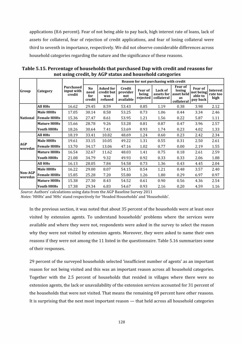
128
applications (8.6 percent). Fear of not being able to pay back, high interest rate of loans, lack of
assets for collateral, fear of rejection of credit applications, and fear of losing collateral were
third to seventh in importance, respectively. We did not observe considerable differences across
household categories regarding the nature and the significance of these reasons.
Table 5.15. Percentage of households that purchased Dap with credit and reasons for not using credit, by AGP status and household categories
Group Category Purchased input with
credit
Reason for not purchasing with credit
No need
for credit
Asked for credit but
was refused
Credit provider
not available
Fear of being
rejected
Lack of assets for collateral
Fear of losing
asset held as
collateral
Fear of not being
able to pay back
Interest rate too
high
National
All HHs 16.62 29.45 8.59 53.43 0.85 1.19 0.38 3.98 2.12
Male HHHs 17.05 30.14 8.58 53.25 0.73 1.06 0.44 3.34 2.46
Female HHHs 15.36 27.47 8.61 53.95 1.21 1.56 0.22 5.87 1.11
Mature HHHs 15.66 28.78 9.26 53.28 0.81 0.87 0.47 3.96 2.57
Youth HHHs 18.26 30.64 7.41 53.69 0.93 1.74 0.23 4.02 1.33
AGP woredas
All HHs 18.19 33.41 10.82 48.69 1.24 0.60 0.23 2.42 2.34
Male HHHs 19.61 33.15 10.05 49.22 1.31 0.55 0.31 2.50 2.61
Female HHHs 13.70 34.17 13.06 47.16 1.02 0.77 0.00 2.19 1.55
Mature HHHs 16.54 32.67 11.62 48.03 1.41 0.75 0.18 2.61 2.59
Youth HHHs 21.08 34.79 9.32 49.93 0.92 0.33 0.33 2.06 1.88
Non-AGP woredas
All HHs 16.13 28.05 7.84 54.58 0.73 1.36 0.43 4.45 2.04
Male HHHs 16.22 29.00 8.07 54.15 0.54 1.21 0.48 3.57 2.40
Female HHHs 15.85 25.28 7.20 55.80 1.26 1.80 0.29 6.97 0.97
Mature HHHs 15.38 27.30 8.43 54.52 0.61 0.90 0.56 4.36 2.54
Youth HHHs 17.38 29.34 6.83 54.67 0.93 2.16 0.20 4.59 1.16
Source: Authors’ calculations using data from the AGP Baseline Survey 2011 Notes: ‘HHHs’ and ‘HHs’ stand respectively for ‘Headed Households’ and ‘Households’.
In the previous section, it was noted that about 35 percent of the households were at least once
visited by extension agents. To understand households’ problems where the services were
available and where they were not, respondents were asked in the survey to select the reason
why they were not visited by extension agents. Moreover, they were asked to name their own
reasons if they were not among the 11 listed in the questionnaire. Table 5.16 summarizes some
of their responses.
29 percent of the surveyed households selected ‘insufficient number of agents’ as an important
reason for not being visited and this was an important reason across all household categories.
Together with the 2.5 percent of households that resided in villages where there were no
extension agents, the lack or unavailability of the extension services accounted for 31 percent of
the households that were not visited. That means the remaining 69 percent have other reasons.
It is surprising that the next most important reason — that held across all household categories

129
— is the fact that farmers did not know there were such services (12.6 percent of the
households in the aggregate sample).

130
Table 5.16. Main reason for not being visited by extension agents, by household categories and AGP status (%)
Group Category
Reason for not being visited by extension agents
Advice they provide is unsuitable
or unhelpful
Not interested
in changing cultivation practices
Do not wish to borrow
money to purchase
inputs
No extension
agent available in this PA
Not enough extension
agents available
in this village
Did not know about
services offered by extension
agents
Extension agents only
help farmers
with more land
Extension agents only help male farmers
Extension agents only
help farmers
with oxen
Extension agents only
help farmers who are
friends or relatives
Extension agents only
help educated farmers
Other
National
All HHs 3.9 5.1 2.5 2.5 28.6 12.6 4.1 1.2 1.3 5 3.9 29.5
Female HHHs 4.1 5.6 2.4 2.1 30.4 11.4 4.4 0.1 0.8 6 4.2 28.5
Male HHHs 3.6 4.0 2.6 3.2 25.0 14.8 3.5 3.3 2.3 3.1 3.2 31.6
Mature HHHs 3.8 4.7 2.4 2.4 28.2 13.6 4.4 1.4 1.3 5 3.9 29
Youth HHHs 4.2 5.7 2.6 2.6 29.1 11.0 3.6 0.8 1.3 5 3.8 30.4
AGP woredas
All HHs 2.0 4.5 2.9 1.7 29.9 15.5 5.0 1.3 1.5 5.4 3.0 27.3
Female HHHs 1.7 3.5 3.5 1.6 26.3 19.2 4.7 3.4 1.5 4.4 2.6 27.6
Male HHHs 2.2 5.1 2.6 1.8 31.7 13.5 5.1 0.2 1.5 5.9 3.2 27.2
Mature HHHs 1.7 3.9 2.6 1.4 31.1 15.8 5.0 1.7 1.4 5.7 3.2 26.5
Youth HHHs 2.6 5.6 3.5 2.2 27.8 14.9 5.0 0.6 1.7 4.9 2.7 28.6
Non-AGP woredas
All HHs 4.5 5.2 2.3 2.7 28.2 11.7 3.8 1.2 1.2 4.8 4.2 30.2
Female HHHs 4.2 4.1 2.2 3.7 24.6 13.4 3.1 3.2 2.6 2.6 3.4 32.9
Male HHHs 4.7 5.8 2.4 2.2 30.0 10.8 4.1 0.1 0.5 6.0 4.6 28.9
Mature HHHs 4.5 4.9 2.4 2.7 27.2 12.9 4.2 1.3 1.2 4.7 4.2 29.7
Youth HHHs 4.6 5.7 2.3 2.7 29.5 9.8 3.2 0.9 1.2 5.0 4.1 31.0
Source: Authors’ calculations using data from the AGP Baseline Survey 2011. Notes: ‘HHHs’ and ‘HHs’ stand respectively for ‘Headed Households’ and ‘Households’. PA stands for Peasant Association

131
Chapter 6: Utilization and Marketing of Crops, Livestock, and
Livestock Products
In this chapter we describe how households use their crop, livestock, and livestock products.
Moreover, we provide descriptions on revenues generated, prices, transportation costs, and
marketing mechanisms involved in selling of their crops, livestock, and livestock products. For
that purpose the chapter is divided into three major sections that respectively deal with crops,
livestock, and livestock products.
6.1. Crop Utilization and Marketing
One of the salient features of crop production in countries such as Ethiopia is that households
consume a significant fraction of the output they harvest. In other words, farmers are largely
subsistent. Thus, in the first subsection we will briefly describe the proportion of each crop
output that is consumed at home, saved for seed, and sold. In the second subsection we describe
revenues generated from crop sales and their variation over the households surveyed. The last
section deals with transportation costs and marketing mechanisms involved in the sales of
crops.
Crop Utilization
In Table 6.1 we summarize utilization rates of the five important cereals (teff, barley, wheat,
maize, and sorghum) as well as nine other crops including pulses, oilseeds, enset, and coffee
14,15. There are significant differences in the proportions consumed and sold among the most
important cereals. Teff is the most marketed cereal with 25 percent of output sold. With 57
percent used for home consumption, teff is also the least home-consumed crop, not only relative
to other cereals but also relative to non-cereals, with the exception of oilseeds and chat. The
four other cereals had a rate of home consumption of at least 60 percent. Seventy-eight percent
of maize output, the most important crop in total crop output, was consumed at home while
only 13 percent of maize production was marketed. At 78.5 percent, a similar proportion of
sorghum is home-consumed while only 10.2 percent is sold. About the same proportion of
barley is sold at 10.8 percent while the proportion consumed at home is slightly lower at 66
percent. Next to teff the cereal with the largest proportion sold is wheat at 17.7 percent and the
proportion of wheat consumed at home is 61 percent.
14
The information on crop use was collected by asking the household how they used the crop production of the year prior to the survey. 15
Note that the reported numbers in Table 6.1. do not add up to 100% because of non-reported categories in the Table (e.g. wastage, animal feed, other uses).

132
The crop with both the largest proportion consumed at home and the lowest proportion
marketed is enset at respective rates of 91.3 and 6.2 percent. Oilseeds and chat, 67.8 and 81.1
percent of which are marketed, constitute the only two crops where less than one-half is home
consumed. Over 63 percent of the coffee produced is consumed at home. However, coffee is the
fourth most marketed crop next to chat, oilseeds, and fruit crops with 34.6 percent of the coffee
produced sold, followed by teff, vegetables, pulses, root crops, and wheat. The proportion of
total output saved as seed for the next season was considerable for barley, wheat, pulses, teff,
root crops, and oil seeds (10-18 percent). The proportion of maize and sorghum saved as seed
was lower (5-6 percent).
Table 6.1 further shows the difference in utilization rates between households with female and
male heads and with mature and young heads. With the exception of enset, female headed
households consumed even larger proportions at home of those crops that have high home
consumption on average (such as cereals, vegetables, and pulses); and they consumed less of
those that are largely for sales, (oilseeds, chat, and coffee). Relative to youth headed households;
mature headed households consumed larger proportions of their output at home (except for
root crops, fruit crops, and enset) and sold less of every item (except for oil seeds and root
crops). Relative to an average household in non-AGP woredas, those in AGP woredas consumed
less (except for teff, chat, and root crops) and sold more of every type of crop (except for teff
and pulses).

133
Table 6.1. Crop use (%), by AGP status, household categories, and crop type (100%=total crop production)
Group Category Variable Teff Barley Wheat Maize Sorghum Pulses Oil
seeds Vege
tables Root
crops Fruit
crops Chat Coffee Enset
National
All HHs Consumption 57.6 66.3 60.9 78.4 78.5 57.1 19.1 71.8 65.0 57.4 17.3 63.7 91.3 Seed 13.2 18.4 18.1 5.5 6.1 15.8 10.2 1.7 10.6 0.6 0.3 0.3 0.3 Sale 25.3 10.8 17.7 12.5 10.2 23.1 67.8 23.9 22.8 38.8 81.1 34.6 6.2
Female HHHs Consumption 60.7 66.7 64.3 82.7 79.1 60.7 17.4 73.2 66.4 62.2 11.4 60.8 89.4 Seed 13.1 17.1 16.9 5.8 6.6 15.3 8.7 1.0 10.7 1.3 0.7 0.1 0.5 Sale 23.3 11.3 15.7 9.1 9.0 19.6 72.1 23.2 21.8 31.3 86.9 37.5 7.8
Male HHHs Consumption 56.6 66.1 59.7 76.7 78.3 55.8 19.6 71.2 64.5 55.6 19.1 64.7 92.1 Seed 13.2 18.8 18.5 5.4 5.9 16.0 10.7 2.0 10.5 0.4 0.1 0.4 0.2 Sale 25.9 10.6 18.3 13.9 10.7 24.3 66.5 24.1 23.1 41.5 79.4 33.6 5.5
Mature HHHs Consumption 58.2 67.3 61.8 79.7 79.4 58.3 20.0 73.5 64.9 57.3 18.1 64.2 91.3 Seed 13.3 18.5 19.0 5.8 6.7 16.0 9.8 1.3 9.9 0.9 0.3 0.3 0.3 Sale 24.9 9.9 15.9 11.7 9.5 22.1 68.0 22.8 23.7 38.5 80.8 34.3 6.1
Youth HHHs
Consumption 56.6 64.5 59.4 76.2 77.0 54.9 17.7 68.5 65.2 57.6 15.8 62.5 91.5
Seed 12.9 18.1 16.5 5.0 5.1 15.3 10.9 2.5 11.9 0.0 0.2 0.3 0.3
Sale 26.0 12.3 20.7 14.0 11.5 25.0 67.3 26.0 21.0 39.3 81.9 35.4 6.2
AGP woredas
All HHs
Consumption 60.2 66.2 58.8 76.5 75.2 55.5 12.4 66.5 65.3 53.2 19.4 58.3 88.7
Seed 14.0 16.8 18.9 6.0 7.1 18.9 9.2 0.8 8.8 0.2 0.9 0.5 0.6
Sale 22.6 13.7 19.8 14.1 14.2 23.0 75.7 30.9 24.5 44.1 77.4 39.8 8.7
Female HHHs
Consumption 64.7 65.7 63.0 80.6 77.9 56.5 13.5 70.6 65.4 51.6 16.1 44.4 87.4
Seed 12.3 16.9 16.8 4.6 6.6 16.5 7.1 0.2 10.3 0.0 2.2 0.5 0.9
Sale 20.9 15.6 18.6 12.6 12.5 25.4 77.7 28.5 23.1 46.9 80.8 54.3 10.3
Male HHHs
Consumption 60.1 64.7 57.2 73.9 74.5 53.6 11.9 65.0 67.3 55.1 20.5 48.4 90.5
Seed 13.8 16.5 19.4 5.3 7.2 17.0 10.6 1.0 7.6 0.3 0.5 0.4 0.3
Sale 21.7 14.8 19.5 16.4 14.7 26.0 74.9 32.3 24.0 42.0 76.3 49.4 7.6
Mature HHHs
Consumption 63.7 67.3 59.5 77.6 75.4 55.4 13.0 67.3 65.7 54.6 19.7 48.1 89.9
Seed 13.4 16.7 19.6 4.9 7.3 17.6 11.2 0.7 8.7 0.3 1.1 0.6 0.4
Sale 20.6 13.5 18.3 14.8 14.8 25.0 73.9 31.0 24.6 42.7 76.9 50.5 7.9
Youth HHHs
Consumption 56.6 60.9 57.1 72.2 75.2 52.3 10.8 65.4 68.8 53.1 18.7 45.4 89.2
Seed 13.6 16.4 17.2 5.3 6.8 15.6 7.8 0.9 7.5 0.0 0.6 0.1 0.5
Sale 23.1 17.3 21.0 16.5 13.1 27.5 78.2 31.6 22.5 44.6 78.5 51.6 9.1
Non-AGP woredas
All HHs
Consumption 56.6 66.3 61.6 79.0 79.5 57.5 21.4 74.3 65.0 58.6 16.4 64.9 92.3
Seed 12.8 18.8 17.8 5.4 5.8 15.1 10.6 2.1 11.1 0.7 0.0 0.3 0.2
Sale 26.4 10.0 17.0 12.0 9.0 23.1 65.0 20.5 22.3 37.2 82.7 33.4 5.3
Female HHHs
Consumption 58.9 67.0 64.9 83.7 79.4 61.9 18.6 74.7 66.7 65.6 9.3 67.1 90.5
Seed 13.5 17.2 17.0 6.4 6.6 14.9 9.1 1.5 10.9 1.8 0.0 0.0 0.3
Sale 24.3 10.0 14.5 7.5 8.1 18.0 70.3 20.3 21.3 26.3 89.6 31.1 6.6
Male HHHs
Consumption 54.7 66.6 60.8 78.1 79.5 56.5 22.9 74.5 63.3 55.7 18.6 70.1 92.9
Seed 12.9 19.7 18.2 5.5 5.5 15.7 10.8 2.5 11.8 0.4 0.0 0.4 0.2
Sale 28.2 9.0 17.8 12.6 9.4 23.8 62.9 19.7 22.8 41.4 80.6 28.4 4.4
Mature HHHs
Consumption 55.4 67.2 62.8 80.7 80.5 59.2 22.9 76.6 64.7 58.1 17.4 70.0 92.0
Seed 13.3 19.2 18.8 6.2 6.5 15.6 9.3 1.6 10.3 1.1 0.0 0.3 0.2
Sale 27.1 8.6 14.9 10.1 8.0 21.2 65.6 18.6 23.3 37.2 82.3 28.5 5.3
Youth HHHs
Consumption 56.5 65.9 60.3 78.2 77.6 55.6 20.2 70.3 63.6 58.9 14.4 68.1 92.7
Seed 12.6 18.7 16.2 4.9 4.6 15.3 12.0 3.5 13.9 0.0 0.0 0.4 0.2
Sale 27.4 10.4 20.6 12.7 10.9 24.2 63.4 22.6 20.4 37.6 83.4 30.2 4.7
Source: Authors’ calculation based on AGP baseline survey, 2011. Note: ‘HHs’ and ‘HHHs’ stand respectively for “Households heads’ and Headed households’.
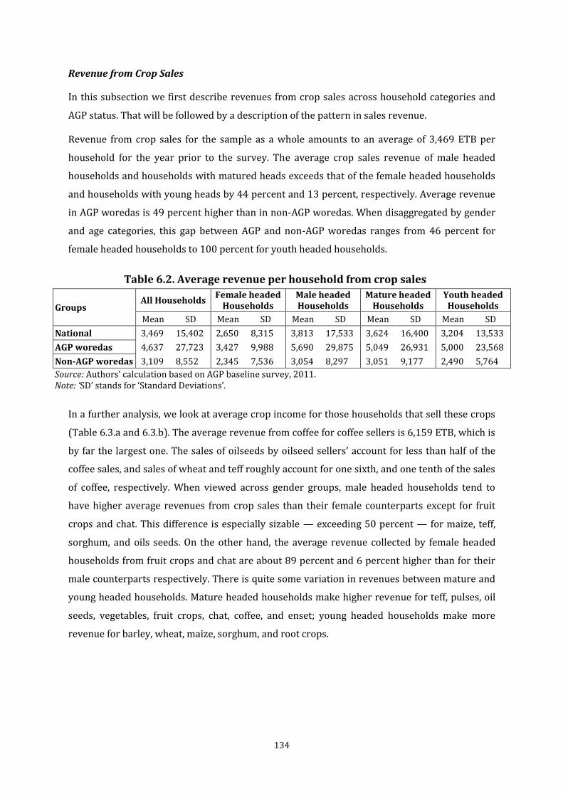
134
Revenue from Crop Sales
In this subsection we first describe revenues from crop sales across household categories and
AGP status. That will be followed by a description of the pattern in sales revenue.
Revenue from crop sales for the sample as a whole amounts to an average of 3,469 ETB per
household for the year prior to the survey. The average crop sales revenue of male headed
households and households with matured heads exceeds that of the female headed households
and households with young heads by 44 percent and 13 percent, respectively. Average revenue
in AGP woredas is 49 percent higher than in non-AGP woredas. When disaggregated by gender
and age categories, this gap between AGP and non-AGP woredas ranges from 46 percent for
female headed households to 100 percent for youth headed households.
Table 6.2. Average revenue per household from crop sales
Groups All Households
Female headed Households
Male headed Households
Mature headed Households
Youth headed Households
Mean SD Mean SD Mean SD Mean SD Mean SD
National 3,469 15,402 2,650 8,315 3,813 17,533 3,624 16,400 3,204 13,533
AGP woredas 4,637 27,723 3,427 9,988 5,690 29,875 5,049 26,931 5,000 23,568
Non-AGP woredas 3,109 8,552 2,345 7,536 3,054 8,297 3,051 9,177 2,490 5,764
Source: Authors’ calculation based on AGP baseline survey, 2011. Note: ‘SD’ stands for ‘Standard Deviations’.
In a further analysis, we look at average crop income for those households that sell these crops
(Table 6.3.a and 6.3.b). The average revenue from coffee for coffee sellers is 6,159 ETB, which is
by far the largest one. The sales of oilseeds by oilseed sellers’ account for less than half of the
coffee sales, and sales of wheat and teff roughly account for one sixth, and one tenth of the sales
of coffee, respectively. When viewed across gender groups, male headed households tend to
have higher average revenues from crop sales than their female counterparts except for fruit
crops and chat. This difference is especially sizable — exceeding 50 percent — for maize, teff,
sorghum, and oils seeds. On the other hand, the average revenue collected by female headed
households from fruit crops and chat are about 89 percent and 6 percent higher than for their
male counterparts respectively. There is quite some variation in revenues between mature and
young headed households. Mature headed households make higher revenue for teff, pulses, oil
seeds, vegetables, fruit crops, chat, coffee, and enset; young headed households make more
revenue for barley, wheat, maize, sorghum, and root crops.

135
Table 6.3.a. Average household revenue, , by household categories, and crop types [for households who sold these crops]
Category Statistics Teff Barley Wheat Maize Sorghum Pulses Oil
seeds Vege
tables Root
crops Fruit
crops Chat Coffee Enset
All HHs
Mean 691 374 1021 532 315 688 2781 372 666 208 1990 6159 66
Median 72 0 0 0 0 7 692 0 0 7 151 0 0
SD 3238 999 2687 1573 1117 1999 34147 1631 2228 1205 9554 19703 214
Female HHs
Mean 469 328 735 233 181 653 1428 315 577 316 2075 5942 64
Median 0 0 0 0 0 0 698 0 0 0 115 0 0
SD 1125 915 1697 745 494 3255 3357 1097 1607 1390 6761 13578 195
Male HHHs
Mean 763 391 1121 654 366 700 3177 395 700 167 1963 6238 67
Median 135 0 0 0 0 21 692 0 0 8 172 0 0
SD 3670 1027 2950 1790 1275 1278 38776 1800 2423 1125 10267 21515 222
Mature HHHs
Mean 740 358 903 501 237 730 3153 377 657 212 2101 6514 68
Median 88 0 0 0 0 0 583 0 0 3 117 0 0
SD 3954 1088 2535 1575 713 2326 42678 1723 2251 935 10301 15439 228
Youth HHHs
Mean 603 403 1228 587 458 606 2196 363 684 199 1773 5461 63
Median 35 0 183 0 0 31 778 0 0 8 205 93 0
SD 1100 826 2924 1568 1605 1129 11737 1437 2181 1615 7903 26116 185
Source: Authors’ calculation based on AGP baseline survey, 2011. Note: ‘HHs’ and ‘HHHs’ stand respectively for Households’ and ‘Headed households’.

136
Table 6.3.b. Average household revenue, by AGP status, household categories, and crop types [for households who sold these crops]
Group Category Statistics Teff Barley Wheat Maize Sorghum Pulses Oil
Seeds Vege
tables Root
Crops Fruit
Crops Chat Coffee Enset
AGP Households
All HHs
Mean 914 536 1260 514 564 914 7982 871 830 267 5626 6636 94
Median 60 0 0 0 0 0 560 0 0 2 91 0 0
SD 1474 735 2410 1582 988 2029 1527 440 1897 860 1419 14245 173
Female HHHs
Mean 554 523 834 388 347 914 3767 502 537 132 5100 5619 83
Median 58 0 183 0 0 138 1666 0 0 11 585 1390 0
SD 939 1610 2322 1086 807 1794 6278 1590 1546 550 10877 13424 231
Male HHHs
Mean 942 595 1236 766 635 999 8290 896 739 302 5802 7513 85
Median 120 0 257 0 0 350 1920 0 0 16 550 2687 0
SD 5833 1501 3316 1840 1577 1835 70671 2867 3060 2253 18602 34288 289
Mature HHHs
Mean 911 565 1060 657 547 1060 8597 865 808 122 6215 6157 86
Median 41 0 84 0 0 275 1666 0 0 11 574 2049 0
SD 6334 1758 3166 1773 1219 1940 78327 2832 3101 398 18564 12003 301
Youth HHHs
Mean 754 604 1269 677 598 820 5457 648 493 524 4584 8682 82
Median 141 0 327 0 0 296 2100 0 0 17 454 1897 0
SD 1483 1024 2964 1489 1732 1574 22285 2063 2109 3306 13735 49626 214
Non-AGP Households
All HHs
Mean 601 333 946 538 238 633 994 135 621 191 489 6046 56
Median 145 0 183 0 0 248 1824 0 0 16 574 379 0
SD 5565 1656 3407 1544 1431 1854 67215 2735 3157 1987 16996 34176 302
Female HHHs
Mean 432 273 693 162 139 578 720 212 589 375 714 6065 55
Median 0 0 0 0 0 0 577 0 0 0 63 0 0
SD 1196 572 1353 505 364 3560 768 669 1626 1561 2664 13634 174
Male HHHs
Mean 669 312 1073 595 278 606 1001 122 684 127 421 5816 58
Median 136 0 0 0 0 0 461 0 0 8 98 0 0
SD 1604 756 2777 1760 1145 1025 1605 569 2087 339 684 15033 177
Mature HHHs
Mean 653 285 835 422 147 629 879 130 600 240 479 6641 59
Median 93 0 0 0 0 0 503 0 0 0 63 0 0
SD 1782 699 2201 1456 436 2423 1374 490 1829 1045 1658 16487 181
Youth HHHs
Mean 527 330 1211 543 411 540 1014 185 769 101 508 4424 52
Median 0 0 0 0 0 0 625 0 0 7 197 0 0
SD 834 727 2907 1603 1557 941 1559 781 2208 241 727 10216 166 Source: Authors’ calculation based on AGP baseline survey, 2011.
137
Note: ‘HHs’ and ‘HHHs’ stand respectively for Households’ and ‘Headed households’. ‘SD’ stands for ‘Standard Deviation’.

138
Except for maize, the average crop revenue of AGP woredas appeared higher than that of the
non-AGP woredas (Table 6.3.b). Within AGP woredas, male headed households reported to have
higher revenue for all the crop categories except for enset (for which the average small revenue
is comparable across gender categories). However, the result is more mixed and there is no
pronounced gap across age categories. A similar pattern is observed within non-AGP woredas.
Comparing AGP and non-AGP woredas across gender and age categories reveals the following.
Similar to the result for all households, male headed households in AGP woredas generated
higher revenue from all crops (even for maize) than in non-AGP woredas. The same holds for
female headed households with the exception that those in AGP woredas earned less revenue
for coffee, fruit crops, and root crops than their counterparts in non-AGP woredas. The general
pattern of higher revenues for AGP households holds also for both age groups, with the
exception that mature headed households in AGP woredas generated less revenue from coffee
and fruit crops than those in non-AGP woredas, and that young headed households in AGP
woredas generated less revenue for root crops than those in non-AGP woredas. Tables 6.3.a and
6.3.b discussed the average household revenue from crop sales for those households who sold
the different crop types. For further analysis, we look into the average revenue from each crop
type for an average household (Table 6.4). In other words, households which did not sell a
certain crop type are considered to have zero revenue from that crop. From such computation,
we find that the average revenue an average household obtains from the sales of crops is about
3,469 ETB. Coffee is the most important crop in total crop sales, accounting for 38 percent of the
total. Wheat is the second most important contributor to total crop sales and the most
important crop in cereal sales. The fact that coffee is the highest contributor to total revenue
holds true to households in both AGP and non-AGP woredas. This significant contribution is due
to the high price of coffee in the market relative to the price of other crops. Although the average
contribution of coffee to total sales is high, the percentage of households that actually sell coffee
is relatively small at 10.4 percent (Annex Table B.6.3). Wheat, the second most important crop
in total crop revenue, is sold by about 15 percent of the households. The marketing of coffee is
also mainly concentrated in Oromiya and SNNP regions (Annex Tables B.6.3 and B.6.4).
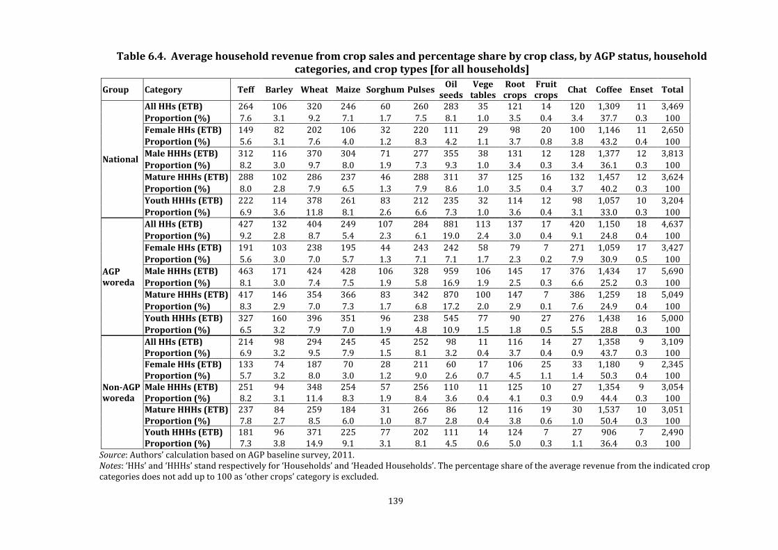
139
Table 6.4. Average household revenue from crop sales and percentage share by crop class, by AGP status, household categories, and crop types [for all households]
Group Category Teff Barley Wheat Maize Sorghum Pulses Oil
seeds Vege
tables Root crops
Fruit crops
Chat Coffee Enset Total
National
All HHs (ETB) 264 106 320 246 60 260 283 35 121 14 120 1,309 11 3,469
Proportion (%) 7.6 3.1 9.2 7.1 1.7 7.5 8.1 1.0 3.5 0.4 3.4 37.7 0.3 100
Female HHs (ETB) 149 82 202 106 32 220 111 29 98 20 100 1,146 11 2,650
Proportion (%) 5.6 3.1 7.6 4.0 1.2 8.3 4.2 1.1 3.7 0.8 3.8 43.2 0.4 100
Male HHHs (ETB) 312 116 370 304 71 277 355 38 131 12 128 1,377 12 3,813
Proportion (%) 8.2 3.0 9.7 8.0 1.9 7.3 9.3 1.0 3.4 0.3 3.4 36.1 0.3 100
Mature HHHs (ETB) 288 102 286 237 46 288 311 37 125 16 132 1,457 12 3,624
Proportion (%) 8.0 2.8 7.9 6.5 1.3 7.9 8.6 1.0 3.5 0.4 3.7 40.2 0.3 100
Youth HHHs (ETB) 222 114 378 261 83 212 235 32 114 12 98 1,057 10 3,204
Proportion (%) 6.9 3.6 11.8 8.1 2.6 6.6 7.3 1.0 3.6 0.4 3.1 33.0 0.3 100
AGP woreda
All HHs (ETB) 427 132 404 249 107 284 881 113 137 17 420 1,150 18 4,637
Proportion (%) 9.2 2.8 8.7 5.4 2.3 6.1 19.0 2.4 3.0 0.4 9.1 24.8 0.4 100
Female HHs (ETB) 191 103 238 195 44 243 242 58 79 7 271 1,059 17 3,427
Proportion (%) 5.6 3.0 7.0 5.7 1.3 7.1 7.1 1.7 2.3 0.2 7.9 30.9 0.5 100
Male HHHs (ETB) 463 171 424 428 106 328 959 106 145 17 376 1,434 17 5,690
Proportion (%) 8.1 3.0 7.4 7.5 1.9 5.8 16.9 1.9 2.5 0.3 6.6 25.2 0.3 100
Mature HHHs (ETB) 417 146 354 366 83 342 870 100 147 7 386 1,259 18 5,049
Proportion (%) 8.3 2.9 7.0 7.3 1.7 6.8 17.2 2.0 2.9 0.1 7.6 24.9 0.4 100
Youth HHHs (ETB) 327 160 396 351 96 238 545 77 90 27 276 1,438 16 5,000
Proportion (%) 6.5 3.2 7.9 7.0 1.9 4.8 10.9 1.5 1.8 0.5 5.5 28.8 0.3 100
Non-AGP woreda
All HHs (ETB) 214 98 294 245 45 252 98 11 116 14 27 1,358 9 3,109 Proportion (%) 6.9 3.2 9.5 7.9 1.5 8.1 3.2 0.4 3.7 0.4 0.9 43.7 0.3 100 Female HHs (ETB) 133 74 187 70 28 211 60 17 106 25 33 1,180 9 2,345 Proportion (%) 5.7 3.2 8.0 3.0 1.2 9.0 2.6 0.7 4.5 1.1 1.4 50.3 0.4 100 Male HHHs (ETB) 251 94 348 254 57 256 110 11 125 10 27 1,354 9 3,054 Proportion (%) 8.2 3.1 11.4 8.3 1.9 8.4 3.6 0.4 4.1 0.3 0.9 44.4 0.3 100 Mature HHHs (ETB) 237 84 259 184 31 266 86 12 116 19 30 1,537 10 3,051 Proportion (%) 7.8 2.7 8.5 6.0 1.0 8.7 2.8 0.4 3.8 0.6 1.0 50.4 0.3 100 Youth HHHs (ETB) 181 96 371 225 77 202 111 14 124 7 27 906 7 2,490 Proportion (%) 7.3 3.8 14.9 9.1 3.1 8.1 4.5 0.6 5.0 0.3 1.1 36.4 0.3 100
Source: Authors’ calculation based on AGP baseline survey, 2011. Notes: ‘HHs’ and ‘HHHs’ stand respectively for ‘Households’ and ‘Headed Households’. The percentage share of the average revenue from the indicated crop categories does not add up to 100 as ‘other crops’ category is excluded.

140
Distribution of Average Household Revenue
Figure 6.1 provides an overview of the variation of revenue from crop sales among households
that actually sold crops. The figure shows that he large majority of households earned much less
revenue than the average income of 4,826 ETB, which had a large standard deviation of 12,191
ETB. To be specific, about one-half of the households earned 597 ETB or less, more than 80
percent earned less than the average revenue, while the upper 5 percent of households earned
14,458 ETB or more. This shows that the average revenue is largely dictated by crop sales
revenue earned by a relatively small proportion of the households.
Figure 6.1. Variation of revenue from crop sales among households that actually sold crops
02
46
81
0
Pe
rcen
t
Mean +1 SD +2 SD +3 SD
0 2000 4000 6000 8000 10000Average household revenue from crop sales
Source: Authors’ calculations using data from the AGP Baseline Survey 2011.
Crop Transportation Costs and Marketing Mechanisms
It is estimated that households paid about 2.2 percent of their total revenue obtained from crop
sales for transportation (Table 6.5). This proportion was smaller among pulses and fruit crops
growers that sold the crops at relatively higher prices and for those farmers that often sell their
products at the local market. The rate of transportation paid by vegetables growers was the
largest at 9 percent of their revenue and much larger than the next highest transportation cost
of 3.8 percent of the revenue of chat growers. This may partly be explained by the special care
needed to transport vegetables as well as the time sensitiveness of the produce. Other crop

141
types with transportation costs in excess of 1 percent of total sales revenue include root crops
(3.2 percent), coffee (2.2 percent), enset (2.2 percent), barley (1.8 percent), and maize (1.7
percent). Note that in addition to the type of crop involved, transportation costs may increase
depending on the location of households relative to marketing centres; and importantly on
whether or not transport operators have to collect the produce from locations relatively close to
each other.
Table 6.5. Percentage of total crop sales' revenue used for transportation, by AGP status, household categories, and crop type
Group Category Teff Barley Wheat Maize Sorghum Pulses Oil
seeds Vege
tables Root
crops Fruit
crops Chat Coffee Enset
National
All HHs 1.0 1.8 1.0 1.7 1.0 0.5 0.9 9.0 3.2 0.5 3.8 2.2 2.2
Female HHHs 1.0 0.9 0.7 1.5 0.9 0.5 0.7 1.1 1.0 0.8 4.8 1.2 2.5
Male HHHs 1.0 2.1 1.1 1.7 1.0 0.6 0.9 9.9 3.9 0.4 3.5 2.6 2.1
Mature HHHs 0.9 2.3 1.1 1.7 0.9 0.5 0.9 1.0 4.7 0.4 4.1 0.8 2.5
Youth HHHs 1.1 0.9 1.0 1.6 1.2 0.7 0.9 12.7 0.8 0.7 3.3 6.5 1.7
AGP woredas
All HHs 0.5 1.3 0.4 1.4 1.6 0.5 1.2 0.7 9.5 0.5 2.6 0.5 1.8
Female HHHs 0.4 1.1 0.5 0.9 2.3 0.5 1.0 0.3 0.9 0.6 3.0 0.5 1.2
Male HHHs 0.4 0.9 0.4 1.0 1.5 0.3 1.3 0.7 9.3 0.5 2.5 0.5 2.0
Mature HHHs 0.4 1.2 0.4 0.9 1.8 0.4 1.3 0.6 10.5 0.7 2.6 0.4 1.9
Youth HHHs 0.5 0.5 0.5 1.2 1.2 0.3 1.1 0.7 1.6 0.1 2.7 0.6 1.4
Non-AGP woredas
All HHs 1.3 2.0 1.4 1.7 0.6 0.6 0.4 13.3 1.2 0.5 5.1 2.7 2.4
Female HHHs 1.5 0.7 0.9 1.8 0.1 0.5 0.2 2.1 1.0 0.9 6.4 1.5 3.3
Male HHHs 1.3 2.7 1.6 2.2 0.7 0.7 0.4 14.3 1.3 0.4 4.7 3.8 2.1
Mature HHHs 1.3 2.7 1.6 2.2 0.3 0.5 0.2 2.1 1.7 0.3 5.7 1.0 2.8
Youth HHHs 1.6 1.2 1.3 2.1 1.2 0.8 0.6 15.3 0.6 1.0 3.9 11.5 1.8
Source: Authors’ calculation based on AGP baseline survey, 2011. Note: ‘HHs’ and ‘HHHs’ stand respectively for ‘Households’ and Headed households’.
Female headed households on average paid 1.4 percent of their crop revenues for
transportation, which is about 40 percent lower than the proportion paid by male headed
households. The average transportation cost of households was inversely related to the age
categories of the heads. While households with mature heads paid 1.7 percent of their revenue
on transportation cost, the corresponding figure for households with young heads was 2.5
percent. Households in non-AGP woredas — which dominantly produce crops costly to
transport — on average paid 2.5 percent of their sales revenue, which is about 48 percent larger
than the 1.7 percent average paid by households in AGP woredas. The finding that the
transportation cost of male headed households and households with young heads exceeds that
of their corresponding counterparts holds for both AGP and non-AGP woredas.

142
The majority households reported to have sold their output to a private trader in the village or
local market, which is what the “Buyer Type I” stands for in the “Major buyer” row of Table 6.6.
Similarly, the majority of the sellers chose the selected buyer for immediate payment reasons,
which is what “immediate pay” stands for in the “Reason to choose buyer” row. The remaining
relatively smaller proportion of households chose their buyer because he/she pays a high price,
and most of the households that chose their buyer because of this reason sold oilseeds. We did
not include the major buyer and reasons for choosing that buyer for all categories (age, gender,
and spatial disaggregation) considered in this report in the table because the first choice of
buyer is the same for all categories and the reason for the choice varied only slightly.
It is interesting to note that households producing the most marketed output, i.e. oilseeds, and
thus are relatively well integrated into the market system can afford to wait relatively longer or
look for a buyer that is willing to pay higher prices. While all households seem to choose traders
over other buyers, most of which are in the local market, the overwhelming majority that are
less integrated to the market chose the buyer with the explicit purpose to get paid immediately.
Whether or not the private trader pays the highest price needs further study. However, the
sellers’ perception is crucial in their decision to whom to sell and it seems to imply that their
immediate need of the money is more important than any other reason.
Only a small proportion of households use mobile phones to communicate with buyers (Table
6.7). This ranged from a rare use of mobile phones among fruit sellers to 11.6 percent for chat
sellers. However, it is interesting to note that among those that use mobile phones the largest
proportion agree on prices over the phone. This result is an important consideration for policy
makers. The lowest proportion is for root crop growers; only 58 percent of the households
selling root crops that used mobile phones agreed on prices on the phone. Next to chat sellers,
vegetable sellers and oil seed sellers are the second and third largest in using mobile phones in
crop sale transactions; however, these proportions are already small with only 4 percent of the
households selling these crops, though, those using the mobile phone in transactions mostly
agree on prices over the phone. While coffee is the most important crop in total crop sales, the
proportion of coffee selling households using the mobile phone for transactions is very low (0.9
percent). This may have to do with the coffee price information that ECX provides.
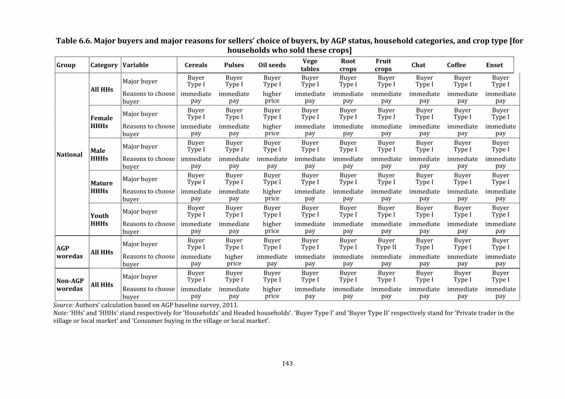
143
Table 6.6. Major buyers and major reasons for sellers’ choice of buyers, by AGP status, household categories, and crop type [for households who sold these crops]
Group Category Variable Cereals Pulses Oil seeds Vege
tables Root crops
Fruit crops
Chat Coffee Enset
National
All HHs Major buyer
Buyer Type I
Buyer Type I
Buyer Type I
Buyer Type I
Buyer Type I
Buyer Type I
Buyer Type I
Buyer Type I
Buyer Type I
Reasons to choose buyer
immediate pay
immediate pay
higher price
immediate pay
immediate pay
immediate pay
immediate pay
immediate pay
immediate pay
Female HHHs
Major buyer Buyer Type I
Buyer Type I
Buyer Type I
Buyer Type I
Buyer Type I
Buyer Type I
Buyer Type I
Buyer Type I
Buyer Type I
Reasons to choose buyer
immediate pay
immediate pay
higher price
immediate pay
immediate pay
immediate pay
immediate pay
immediate pay
immediate pay
Male HHHs
Major buyer Buyer Type I
Buyer Type I
Buyer Type I
Buyer Type I
Buyer Type I
Buyer Type I
Buyer Type I
Buyer Type I
Buyer Type I
Reasons to choose buyer
immediate pay
immediate pay
immediate pay
immediate pay
immediate pay
immediate pay
immediate pay
immediate pay
immediate pay
Mature HHHs
Major buyer Buyer Type I
Buyer Type I
Buyer Type I
Buyer Type I
Buyer Type I
Buyer Type I
Buyer Type I
Buyer Type I
Buyer Type I
Reasons to choose buyer
immediate pay
immediate pay
higher price
immediate pay
immediate pay
immediate pay
immediate pay
immediate pay
immediate pay
Youth HHHs
Major buyer Buyer Type I
Buyer Type I
Buyer Type I
Buyer Type I
Buyer Type I
Buyer Type I
Buyer Type I
Buyer Type I
Buyer Type I
Reasons to choose buyer
immediate pay
immediate pay
higher price
immediate pay
immediate pay
immediate pay
immediate pay
immediate pay
immediate pay
AGP woredas
All HHs Major buyer
Buyer Type I
Buyer Type I
Buyer Type I
Buyer Type I
Buyer Type I
Buyer Type II
Buyer Type I
Buyer Type I
Buyer Type I
Reasons to choose buyer
immediate pay
higher price
immediate pay
immediate pay
immediate pay
immediate pay
immediate pay
immediate pay
immediate pay
Non-AGP woredas
All HHs Major buyer
Buyer Type I
Buyer Type I
Buyer Type I
Buyer Type I
Buyer Type I
Buyer Type I
Buyer Type I
Buyer Type I
Buyer Type I
Reasons to choose buyer
immediate pay
immediate pay
higher price
immediate pay
immediate pay
immediate pay
immediate pay
immediate pay
immediate pay
Source: Authors’ calculation based on AGP baseline survey, 2011. Note: ‘HHs’ and ‘HHHs’ stand respectively for ‘Households’ and Headed households’. ‘Buyer Type I’ and ‘Buyer Type II’ respectively stand for ‘Private trader in the village or local market’ and ‘Consumer buying in the village or local market’.

144
Table 6.7. Proportion of households that used mobile phones in crop sale transaction and that agreed prices over the mobile phone, if used, by AGP status, household categories, and crop type [for households who sold these crops]
Group Category Variable Cereals Pulses Oil
seeds Vege
tables Root
crops Fruit
crops Chat Coffee Enset
National
All HHs Mobile use in crop sale (%) 2.2 1.9 3.8 3.9 2.6 0.1 11.6 0.9 2.5
Agreed price over mobile (%) 90.7 82.6 99.5 97.0 58.3 0.0 87.6 100 100
Female HHHs
Mobile use in crop sale (%) 1.4 1.2 2.0 0.8 4.8 0.0 7.6 0.0 3.1
Agreed price over mobile (%) 98.2 66.9 96.3 100 37.1
100.0
100
Male HHHs
Mobile use in crop sale (%) 2.4 2.2 4.3 4.9 1.8 0.1 12.9 1.3 2.2
Agreed price over mobile (%) 89.3 85.3 100 96.8 78.1 0.0 85.1 100 100
Mature HHHs
Mobile use in crop sale (%) 2.0 2.1 4.3 0.7 3.7 0.0 9.6 1.1 3.8
Agreed price over mobile (%) 98.1 91.1 100 83.5 55.7
99.5 100 100
Youth HHHs
Mobile use in crop sale (%) 2.5 1.7 2.9 8.4 0.7 0.2 15.3 0.4 0.0
Agreed price over mobile (%) 80.8 65.2 98.4 98.5 81.6 0.0 73.4 100
AGP woredas
All HHs Mobile use in crop sale (%) 2.1 3.9 1.9 0.9 4.2 0.3 1.1 0.6 1.3
Agreed price over mobile (%) 82.7 76.0 97.2 100 92.9 0.0 91.1 100 100
Non-AGP woredas
All HHs Mobile use in crop sale (%) 2.2 1.2 4.7 6.0 2.0 0.0 16.0 1.0 3.1
Agreed price over mobile (%) 95.2 89.8 100 96.6 29.8
87.5 100 100
Source: Authors’ calculation based on AGP baseline survey, 2011. Note: ‘HHs’ and ‘HHHs’ stand respectively for ‘Households’ and ‘Headed households’.

145
6.2. Livestock Marketing
The households in the four regions included in the AGP survey practice a mixed crop-livestock
production system. These regions also account for a large majority of the livestock population in the
country. As discussed in Chapter 2, livestock is an important part of household assets, which is
monetized when households sell their livestock in times of need. Households also benefit from the
flow of outputs that their stock provides in the form of milk and dairy products, eggs, and hides and
skins. Moreover, the services cattle provide in ploughing the land is a crucial input in crop
production. This section deals with livestock sales focusing on revenue generated and marketing
mechanisms. The first subsection deals with livestock revenue while the second deals with
transportation costs and marketing mechanisms.
Revenues from Livestock Sales
The revenue from livestock sales for an average household in the survey makes up to 1,344 ETB in
the year prior to the survey (Table 6.8). Revenue from sales income from livestock constitutes 38
percent of the revenue from crop sales. Within the sales of livestock, it is especially the sales of
cattle which are important as they account for 77 percent of the total sales. Second come the sales
of goats and sheep accounting for 13 percent of total livestock sales income. Pack animals and
chickens each count for 5 percent of total sales income.
The numbers in Table 6.8 further indicate that households with male heads generated 34 percent
more income from all livestock sales than female headed households. When we compare this for the
different livestock categories, we note that male headed households, compared to female headed
households, earn 49 percent more income from cattle sales, 32 percent more from sheep and goats,
and 334 percent more from pack animals. In contrast, female headed households generated 385
percent more from chicken sales. Relative to households with young heads, those with mature
heads earned more income from the sales of all livestock types (with the exception of sheep and
goats and camels). Mature headed households earned 8, 65, and 132 percent more relative to
households with young heads from the sales of cattle, pack animals, and chickens, respectively,
while the average revenue collected from the sale of sheep and goats is comparable. As a result of
this, total livestock earning of mature headed households was 12.3 percent larger relative to that of
households with young heads. On average, households in AGP woredas earned 801 ETB from cattle
sales, which was 28 percent lower relative to the mean revenue of 1,111 ETB obtained by
households in non-AGP woredas. For all livestock types, the revenues are smaller for households in

146
AGP woredas compared to those in non-AGP woredas.
Table 6.8. Average and proportion of revenue collected from sale of livestock products, by household category, AGP status, and livestock type
Category Statistics Cattle Sheep
& goats Pack
animals Chickens Total
All Households Average Revenue (ETB) 1,037 177 64 64 1,344
Proportion (%) 77 13 5 5 100
Female headed Households
Average Revenue (ETB) 768 144 19 148 1,080
Proportion (%) 71 13 2 14 100
Male headed Households
Average Revenue (ETB) 1,144 190 82 31 1,449
Proportion (%) 79 13 6 2 100
Mature headed Households
Average Revenue (ETB) 1,066 177 75 81 1,401
Proportion (%) 76 13 5 6 100
Youth headed Households
Average Revenue (ETB) 987 176 45 35 1,248
Proportion (%) 79 14 4 3 100
AGP woredas Average Revenue (ETB) 801 155 49 30 1,044
Proportion (%) 77 15 5 3 100
Non-AGP woredas
Average Revenue (ETB) 1,111 184 69 75 1,438
Proportion (%) 77 13 5 5 100
Source: Authors’ calculation based on AGP baseline survey, 2011.
Livestock Transportation Costs and Marketing Mechanisms
One of the most commonly cited reasons for low monetization and productivity of the livestock
sector is poor infrastructure such as roads and telecommunication. In this subsection, we describe
the cost of transportation, the intensity of mobile use in livestock marketing, and its role in price
determination. A description about households’ main livestock buyers in the survey areas and the
main reasons for their choices of the buyers is also included. To directly link transportation cost to
the amount generated from the sale of livestock, we focus here on the proportion of revenue paid
for transportation, which we summarize in Table 6.9. Caution is in order in interpreting the
magnitude of this variable. A transportation cost that is a smaller proportion of total revenue does
not necessarily imply that the market is closer. Whenever roads or transportation means are not
available, farmers have to travel to the market places on foot and the opportunity cost of time is not
included in this analysis.
Table 6.9 shows that households paid an average of about 0.3 percent of their total revenue
obtained from livestock sales for transportation. This ranges from nearly 0.1 percent for pack
animals to 0.5 percent for chickens. Compared to the proportion of total revenue spent on

147
transporting crops, this is smaller as households often trek with their cattle to markets as opposed
to crops that have to be transported. The latter also partially explains the relatively higher
transportation cost of chickens.
Female headed households on average spent 0.1 percent of the revenue they generated from
livestock sales on transportation, while male headed households on average paid 0.3 percent. Recall
that also in the case of crops transportation fares accounted for a larger proportion of total revenue
for male headed households than for female headed households. It also seems that, on average,
transportation cost relative to revenue was slightly higher for households with younger heads
compared the households with mature heads. Households in non-AGP woredas paid on average 0.3
percent of their sales revenue on transportation which ranges from 0.1 percent on pack animals to
0.8 percent on chicken. As is shown in Table 6.9, the proportion of revenue spent on transporting
livestock is higher for all livestock categories in non-AGP woredas than in AGP woredas where
households on average paid about 0.1 percent of their revenue for transportation.
Table 6.9. Proportion of revenue paid for transportation, by household and livestock category and AGP status
Category Cattle Sheep &
goats Pack
animals Chickens
All Households 0.3 0.2 0.1 0.5
Female headed Households 0.1 0.1 0.1 0.5
Male headed Households 0.3 0.3 0.1 0.5
Mature headed Households 0.1 0.2 0.1 0.7
Youth headed Households 0.5 0.3 0.0 0.2
AGP woredas 0.1 0.1 0.1 0.1
Non-AGP woredas 0.3 0.3 0.1 0.8 Source: Authors’ calculation based on AGP baseline survey, 2011.
Local markets or buyers/consumers in the village were the major destinations for households'
livestock sales followed by buyers/sellers in the region and local consumers. Figure 6.2 shows that
these three buyers jointly accounted for more than 85 percent of the total sales for all livestock
categories, except camels.16 This was consistent across livestock groups, household categories, and
AGP and non-AGP woredas.
16
For camels, the major buyers were not clearly identified in the survey.
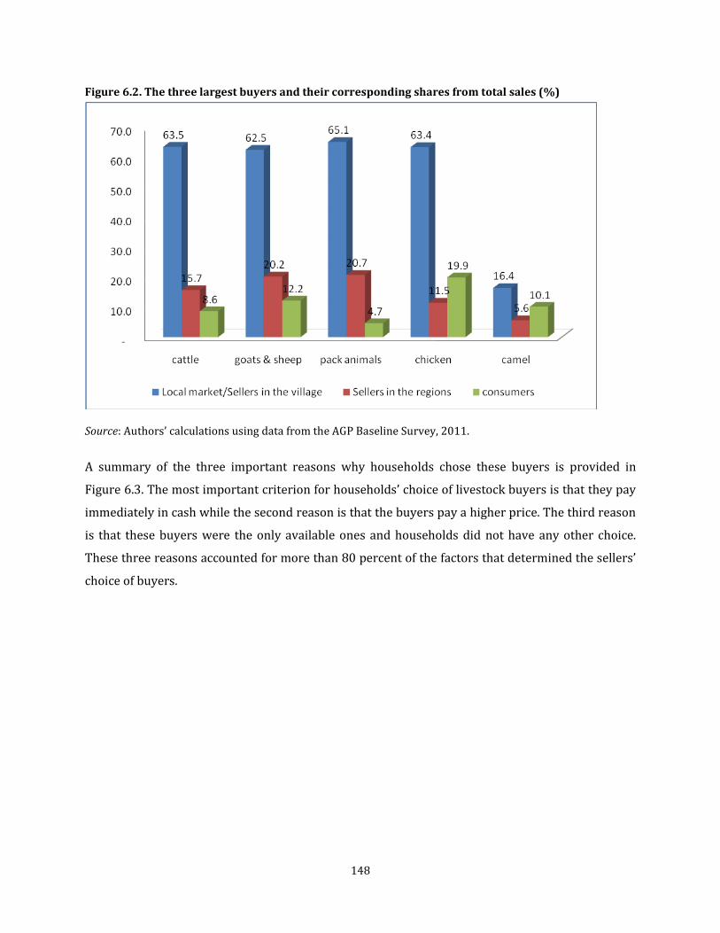
148
Figure 6.2. The three largest buyers and their corresponding shares from total sales (%)
Source: Authors’ calculations using data from the AGP Baseline Survey, 2011.
A summary of the three important reasons why households chose these buyers is provided in
Figure 6.3. The most important criterion for households’ choice of livestock buyers is that they pay
immediately in cash while the second reason is that the buyers pay a higher price. The third reason
is that these buyers were the only available ones and households did not have any other choice.
These three reasons accounted for more than 80 percent of the factors that determined the sellers’
choice of buyers.

149
Figure 6.3. The three most important reasons for sellers' choice of buyer and their corresponding shares (%)
Source: Authors’ calculations using data from the AGP Baseline Survey 2011.
Though mobile phone usage has considerably increased in the country, its usage to facilitate
livestock sales transactions is limited. Table 6.10 summarizes the proportion of households that
used mobile phone to contact their buyers and the proportion that agreed on a price over the phone
from those reported to have used a mobile phone in transactions. The numbers in the table indicate
that only 0.8 percent of the total sample used a mobile phone in livestock sales. This differs among
different livestock categories with 0.1 percent for chicken and sheep and goats, 1.3 percent for
cattle, and 4.3 percent for pack animals. It is, however, important to note that among those that
used mobile phone to contact their buyers, about 54 percent agreed on a price over the phone.

150
Table 6.10. Proportion of households that used mobile phone for livestock sales transaction and those that agreed on a price on the phone, if used, by household
categories, AGP status, and livestock categories
Group Category Variable Cattle Sheep &
goats Pack
animals Chickens
National
All HHs Mobile use in sale (%) 1.3 0.1 4.3 0.1
Agreed price over mobile (%) 56.6 43.5 49.6 56.7
Female HHHs
Mobile use in sale (%) 0.3 0.2 1.1 0.0
Agreed price over mobile (%) 39.1 48.4 0.0 100
Male HHHs
Mobile use in sale (%) 1.6 0.1 4.9 0.1
Agreed price over mobile (%) 57.7 41.9 51.5 51.4
Mature HHHs
Mobile use in sale (%) 1.5 0.2 4.0 0.1
Agreed price over mobile (%) 69.2 58.1 81.4 100
Youth HHHs
Mobile use in sale (%) 1.1 0.1 4.8 0.1
Agreed price over mobile (%) 24.3 0.0 7.2 0.0
AGP woredas
All HHs Mobile use in sale (%) 1.3 0.6 5.1 0.3
Agreed price over mobile (%) 43.2 43.5 22.8 56.7
Non-AGP woredas
All HHs Mobile use in sale (%) 1.4 0.0 4.1 0.0
Agreed price over mobile (%) 62.2 59.8 56.7
Source: Authors’ calculation based on AGP baseline survey, 2011. Note: ‘HHs’ and ‘HHHs’ stand respectively for ‘Households’ and ‘Headed households’.
Comparing the sub-samples, a larger proportion of male headed households used the mobile phone,
which held true across all livestock categories, and they agreed more frequently on a sales price
over the phone relative to female headed households, except for goats and sheep. Interestingly, on
average, the use of mobile phones in livestock transactions is a little more common among
households with young heads than those with mature heads. This probably suggests that
households with younger heads are relatively more attracted to modern ways of doing business.
In AGP woredas, the proportion of households that used mobile phone to contact buyers was 1.1
percent. This is slightly higher than the 0.8 percent mobile usage in households in non-AGP
woredas. On the other hand, while about 40 percent of those who had contact with buyers agreed
price over the phone in AGP woredas, a relatively larger proportion of 62 percent agreed prices in
non-AGP woredas.
Revenues from Livestock Products
In this part, we briefly describe the revenues generated from livestock products. The livestock
products covered in the survey are meat (excluding the sale of live animals), hides/skins,
butter/yoghurt, eggs, milk/cream, and dung. For the 12 months prior to the survey, an average
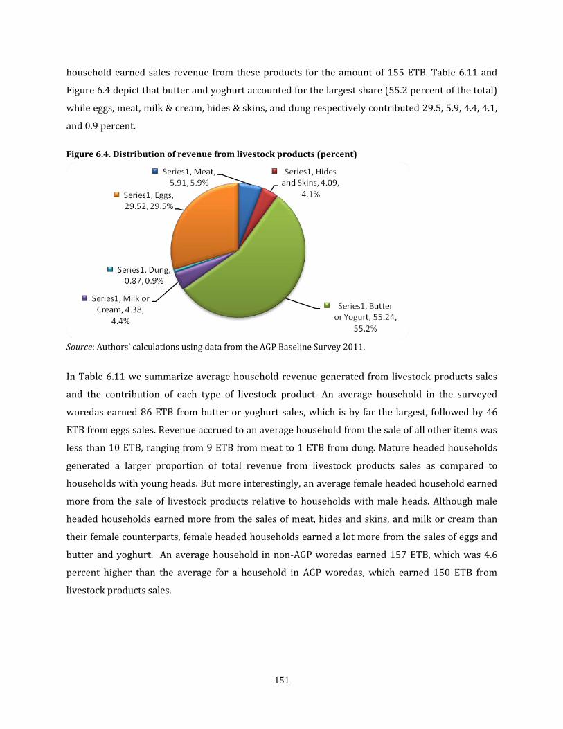
151
household earned sales revenue from these products for the amount of 155 ETB. Table 6.11 and
Figure 6.4 depict that butter and yoghurt accounted for the largest share (55.2 percent of the total)
while eggs, meat, milk & cream, hides & skins, and dung respectively contributed 29.5, 5.9, 4.4, 4.1,
and 0.9 percent.
Figure 6.4. Distribution of revenue from livestock products (percent)
Source: Authors’ calculations using data from the AGP Baseline Survey 2011.
In Table 6.11 we summarize average household revenue generated from livestock products sales
and the contribution of each type of livestock product. An average household in the surveyed
woredas earned 86 ETB from butter or yoghurt sales, which is by far the largest, followed by 46
ETB from eggs sales. Revenue accrued to an average household from the sale of all other items was
less than 10 ETB, ranging from 9 ETB from meat to 1 ETB from dung. Mature headed households
generated a larger proportion of total revenue from livestock products sales as compared to
households with young heads. But more interestingly, an average female headed household earned
more from the sale of livestock products relative to households with male heads. Although male
headed households earned more from the sales of meat, hides and skins, and milk or cream than
their female counterparts, female headed households earned a lot more from the sales of eggs and
butter and yoghurt. An average household in non-AGP woredas earned 157 ETB, which was 4.6
percent higher than the average for a household in AGP woredas, which earned 150 ETB from
livestock products sales.

152
Table 6.11. Average revenue and share of different categories in total revenue of livestock products
Category Statistics Meat Hides &
skins Butter or yoghurt
Milk or cream
Dung Eggs Total
All HHs Average Revenue (ETB) 9.2 6.3 85.8 6.8 1.4 45.8 155
Proportion (%) 5.9 4.1 55.2 4.4 0.9 29.5 Female
HHHs Average Revenue (ETB) 4.4 3.2 96.0 4.5 0.9 53.9 163
Proportion (%) 2.7 2.0 59.0 2.7 0.5 33.1
Male HHHs Average Revenue (ETB) 11.2 7.7 81.4 7.8 1.6 42.4 152
Proportion (%) 7.4 5.1 53.5 5.1 1.0 27.9 Mature
HHHs Average Revenue (ETB) 9.5 7.4 109.8 7.1 1.6 47.2 183
Proportion (%) 5.2 4.0 60.1 3.9 0.9 25.9 Youth
HHHs Average Revenue (ETB) 8.6 4.5 41.6 6.2 0.9 43.3 105
Proportion (%) 8.2 4.3 39.6 5.9 0.9 41.3 AGP
woredas Average Revenue (ETB) 10.3 9.6 71.6 24.7 2.5 31.4 150
Proportion (%) 6.9 6.4 47.7 16.5 1.7 20.9 Non-AGP
woredas Average Revenue (ETB) 8.8 5.3 90.2 1.2 1.0 50.4 157
Proportion (%) 5.6 3.4 57.5 0.8 0.6 32.1 Source: Authors’ calculation based on AGP baseline survey, 2011.
Note: ‘HHs’ and ‘HHHs’ stand respectively for ‘Households’ and ‘Headed households’.
6.3. Dairy Marketing
Table 6.12 shows that households that sell dairy products had to travel about 52 minutes on
average to a market place. For those that paid transportation costs, this translates into 1.1 percent
of total revenue, on average. The disaggregated figures show that the proportion of total revenue
spent on transportation is consistently and notably lower for female headed households, relative to
the male headed households, regardless of the distance they travel to the market place. For non-
AGP woredas, the average travel time to the market place was 55 minutes ranging from 43 minutes
for yoghurt to 69 minutes for butter. The corresponding share of transportation costs to total
revenue averages 2 percent. On the other hand, for AGP woredas, the average distance to the
market place was about 42 minutes with the proportion paid for transportation costs amounting to
about 0.5 percent.

153
Table 6.12. Average travel time to the market place and proportion of revenue paid for transportation, by household category and AGP status
Category Statistics Fresh milk Cheese Butter Yoghurt
All HHs Proportion paid for transportation (%) 1.4 2.4 0.7 0.0
Average travel time to market (minutes) 50.0 48.6 65.4 43.4
Female HHHs Proportion paid for transportation (%) 0.7 0.5 0.4 0.0
Average travel time to market (minutes) 62.5 48.4 63.0 40.0
Male HHHs Proportion paid for transportation (%) 1.6 3.6 0.8 0.0
Average travel time to market (minutes) 45.7 48.7 66.5 48.6
Mature HHHs Proportion paid for transportation (%) 0.3 2.1 0.7 0.0
Average travel time to market (minutes) 45.6 49.0 66.3 38.1
Youth HHHs Proportion paid for transportation (%) 3.2 3.1 0.7 0.0
Average travel time to market (minutes) 55.0 47.8 64.0 52.7
AGP woredas Proportion paid for transportation (%) 0.9 0.6 0.4 0.0
Average travel time to market (minutes) 29.4 41.5 51.8 45.9
Non-AGP woredas
Proportion paid for transportation (%) 1.6 3.2 0.9 0.0
Average travel time to market (minutes) 55.1 51.0 69.1 43.0
Source: Authors’ calculation based on AGP baseline survey, 2011. Note: ‘HHs’ and ‘HHHs’ stand respectively for ‘Households’ and ‘Headed Households’.
Analogous to livestock and crops, local markets or buyers/consumers in the village, buyers/sellers
in the region, and local consumers were the major buyers of dairy products. Figure 6.5 summarizes
the proportion by the three buyers in each type and in total. It shows that the three buyers jointly
counted for about 94 percent and local markets alone command about one half of the total market
of dairy products. Consumers and regional traders rank second and third with an average share of
32.1 percent and 12.2 percent, respectively. By and large, this is the pattern for all types of dairy
products and for all demographic and spatial categories considered in this report.

154
Figure 6.5. The three largest buyers of dairy products and their share from total sales
Source: Authors’ calculations using data from the AGP Baseline Survey 2011.
Similar to the case of crops and livestock in general, the major reasons for the households’ choice of
buyers are ‘pay immediately’ and ‘pay better/higher prices’ (see Figure 6.6). The figure also
indicates that sizable proportions of the households do not have alternative buyers to choose from.
Figure 6.6. The three most important reasons for choices of dairy product buyers and their respective share
Source: Authors’ calculations using data from the AGP Baseline Survey 2011.

155
6.4. Summary
Sales income. Combining sales revenue from three sources (crops, livestock, and livestock
products), it is found that total sales income for an average household in the survey area over a 12
month period amounts to 4,968 ETB. The majority of the sales revenue is made up from crop sales,
as this category accounts for 70 percent of the sales income of the average household (3,469 ETB).
Second comes the revenue from the sales of livestock, making up 26 percent of the sales income
(1,344 ETB). Sales revenue from livestock products (meat, hides and skins, milk, cheese, butter,
yoghurt, dung, and eggs) are estimated to be relatively less important as they make up only 3
percent of the annual sales revenue of an average household (155 ETB).
Crop utilization. One of the salient features of crop production in countries such as Ethiopia is that
households consume a significant fraction of the output they harvest. This is also found in this
dataset. We, however, note significant differences between crops. Only for two crops more than half
of the production is sold, i.e. chat (81 percent) and oilseeds (68 percent). Even for a major cash crop
as coffee, the majority of the production is consumed by the household itself (64 percent) and only
35 percent of the coffee production is put up for sale. We note also large differences between the
major cereals. Of all the cereals, teff is used most as a cash crop. A quarter of total production is
being sold. This compares to 58 percent of its production being used for own consumption.
Sorghum, maize, and barley show the lowest level of commercialization with a share of production
that is being sold ranging from 10 percent to 13 percent. Farmers in the study area further rely
little on markets to obtain seeds, as illustrated by relatively large percentages being retained for
seed purposes, in the case of cereals varying between 6 percent (maize) and 19 percent (barley) of
total household production.
Crop sales. The average revenue from crop sales in the survey area in the year prior to the survey
amounts to 3,469 ETB per household. There are large differences between households and it is
estimated that 50 percent of the households earned less than 597 ETB from crops sales. Coffee is
the most important crop in total crop revenue, accounting for 40 percent of total crop sales
revenue, followed by wheat accounting for 11 percent of the total crop sales revenue. This high
contribution of coffee to total crop sales revenue could be driven by the high price of coffee relative
to other crops. However, only 10 percent of the households are marketing coffee and are mainly
concentrated in SNNP and Oromiya regions. Most of the crops are being sold to village traders and

156
few farmers travel far distances to sell produce as it is found that transportation costs make up a
relatively small percentage of total sales earnings. Most importantly, most farmers chose buyers
because they are able to pay immediately and not because they offer higher prices. This might
reflect lack of trust in buyers as well as a relative large importance of distress sales. It is also found
that few farmers use mobile phones for their sales transactions, partly reflecting the still relatively
low penetration of mobile phones in rural areas of Ethiopia. If farmers use a mobile phone in
transactions they often agree on prices on the phone.
Livestock sales. The revenue from livestock sales for an average household in the survey made up to
1,344 ETB in the year prior to the survey. Revenue from livestock sales constitutes 38 percent of
the revenue from crop sales. Within the sales of livestock, it is especially the sales of cattle that are
important as they account for 77 percent of the total sales revenue. The sale of goats and sheep
comes second accounting for 13 percent of total livestock sales revenue. Pack animals and chicken
each count for 5 percent of total livestock sales revenue. As for the case of crops, expenses for
transportation are a small proportion of the livestock sales revenue. The most important reason for
choosing a buyer is linked to immediate cash payments, followed by the prices offered. No choice in
traders is relatively less important as the reason for the choice of a particular trader, but it still
makes up 10 percent of the stated answers for choosing a trader. It thus seems that farmers in these
surveyed areas might benefit from improved choices in sales options.
Livestock products. The revenues that were generated from the sales of livestock products
amounted to 155 ETB for an average household in the year prior to the survey. The most important
livestock product was the butter/yoghurt category accounting for 55 percent of all sales income in
this category. Second came eggs, accounting for 30 percent. Meat (6 percent), hides and skins (4
percent), fresh milk or cream (4 percent), and dung (1 percent) are relatively much less important.
While sales to village traders are still relatively most important, direct sales to consumers for these
products are much more important than for crop and livestock sales, reflecting the more perishable
nature of the majority of these products. They are thus probably relatively more important for the
local economy. The most important reason for the choice of a buyer is again immediate cash
payments (and less the level of the price offered).

157
Chapter 7: Wage Employment and Nonfarm Businesses
7.1. Participation in Wage Employment and Nonfarm Business
Although farming on own agricultural land is the major activity of households in rural Ethiopia,
some rural households are also engaged in wage employment or nonfarm businesses. In the AGP
baseline survey, households were asked if any of their members participated in any wage
employment or nonfarm businesses and the type of activity they were engaged in. Figure 7.1
presents the percentage of households who participate in wage employment or nonfarm
businesses. In 30 percent of the households either the head or other members in the households
were engaged in some sort of wage employment. In half of the cases, it is the head only that
participated in such activities while in close to 10 percent of the households it is the head and at
least one other member that are engaged in wage employment. In the remaining 5 percent of the
households, only other members of the households have some participation. In only 24 percent of
the households head or other members were engaged in nonfarm business. This could be due to the
capital requirement of starting one’s own business as opposed to wage employment which does not
have any capital requirement. In 12 percent of the cases, the nonfarm businesses are owned and
operated by the household heads. In the remaining 8 and 4 percent the businesses are owned by
other members only, and by the head and other members together, respectively.
Figure 7.1. Percentage of households with wage employment and nonfarm businesses
Source: Authors’ calculations using data from the AGP Baseline Survey 2011.
When looking into the characteristics of households that engage in wage employment or nonfarm
businesses, the percentage of households engaged in such activities is higher for male headed

158
households compared to the female headed ones. The percentage difference is particularly higher
for wage employment (8.2 percent more) compared to the difference in terms of being engaged in
nonfarm businesses (6.5 percent more). There is a 6.3 percent difference between households with
mature heads and households with younger heads in wage employment. However, the difference is
about 9 percent for those engaged in nonfarm businesses. This could be a reflection of the risk
taking behaviour of younger household heads compared to the mature heads.
The percentage of households in AGP woredas engaged in wage employment is slightly higher than
those in non-AGP woredas while for nonfarm businesses the reverse is true. However, the pattern
in terms of the difference between female and male headed households, and young and mature
heads is similar in both woreda categories, i.e. male headed and young headed households in both
AGP and non-AGP woredas are engaged more in wage employment and nonfarm business
compared to their respective counterparts.
Table 7.1. Percentage of households with wage employment or nonfarm businesses, by household categories and AGP status
Group Category Wage employment Nonfarm business
National
All HHs 30.4 24.2
Female HHHs 24.6 19.6
Male HHHs 32.8 26.1
Mature HHHs 28.0 20.8
Youth HHHs 34.3 29.9
AGP- woredas
All HHs 30.8 19.7
Female HHHs 22.2 19.6
Male HHHs 31.9 19.8
Mature HHHs 25.9 16.9
Youth HHHs 34.3 24.6
Non-AGP woredas
All HHs 29.0 25.6
Female HHHs 25.4 19.7
Male HHHs 33.1 28.1
Mature HHHs 28.7 22.0
Youth HHHs 34.3 31.4
Source: Authors’ calculations using data from the AGP Baseline Survey 2011. Note: ‘HHHs’ and ‘HHs’ stand respectively for ‘Headed households’ and ‘Households’.

159
7.2. Types of Wage Employment and Nonfarm Business Activities
Wage Employment Activities
Figure 7.2 presents the type of activities households are engaged in by AGP woreda classification.
The most common wage employment type is working on agricultural farms for cash or in-kind
payments. From those households who indicated that they were engaged in some sort of wage
employment activities, 63 percent were working in agriculture. The next common employment
activity, practiced by about 23 percent of the households, was unskilled nonfarm work which may
include casual works not related with agricultural production. Professional or skilled work
accounted for 8 percent of the households. A slightly higher percentage of households in non-AGP
woredas were engaged in both unskilled nonfarm work and professional work.
Figure 7.2. Percentage of households, by type of wage employment and
AGP status [for households that earn wages]
Source: Authors’ calculations using data from the AGP Baseline Survey 2011.
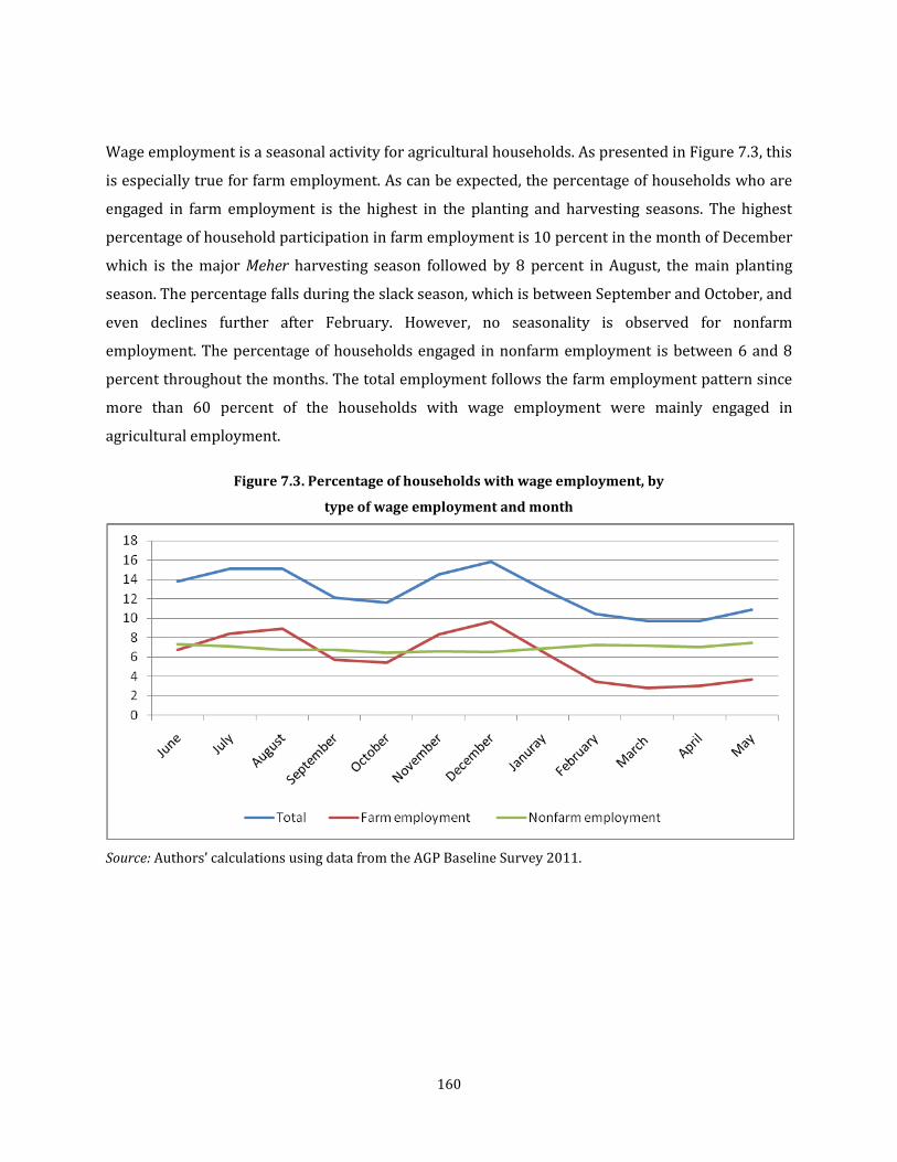
160
Wage employment is a seasonal activity for agricultural households. As presented in Figure 7.3, this
is especially true for farm employment. As can be expected, the percentage of households who are
engaged in farm employment is the highest in the planting and harvesting seasons. The highest
percentage of household participation in farm employment is 10 percent in the month of December
which is the major Meher harvesting season followed by 8 percent in August, the main planting
season. The percentage falls during the slack season, which is between September and October, and
even declines further after February. However, no seasonality is observed for nonfarm
employment. The percentage of households engaged in nonfarm employment is between 6 and 8
percent throughout the months. The total employment follows the farm employment pattern since
more than 60 percent of the households with wage employment were mainly engaged in
agricultural employment.
Figure 7.3. Percentage of households with wage employment, by
type of wage employment and month
Source: Authors’ calculations using data from the AGP Baseline Survey 2011.

161
Table 7.2 below presents the percentage of households in each wage employment activity by
household characteristics (percentages calculated from those households who indicated that at
least one member is engaged in wage employment). The percentage of households who have at
least one member employed in farming is slightly higher for female headed households (66
percent) compared to male headed households (62 percent). In contrast, 9 percent more male
headed households participate in professional or skilled work compared to female headed
households.
Table7.2. Percentage of households, by type of wage employment, by household categories, and AGP status [for households that earn wages]
Group Category Farming on
others' farm
Unskilled nonfarm
work
Professional or skilled
work
Food for work
program Soldier Other
National
All HHs 62.8 23.5 8.0 4.6 0.6 6.4
Female HHHs 65.8 26.0 1.5 4.6 0.4 6.2
Male HHHs 61.8 22.6 10.4 4.6 0.7 8.8
Mature HHHs 65.2 22.4 7.8 4.2 0.3 8.3
Youth HHHs 59.5 25.0 8.3 5.2 1.1 7.9
AGP woredas
All HHs 65.1 20.4 5.9 3.9 1.6 6.9
Female HHHs 61.1 22.1 5.0 5.5 0.3 7.9
Male HHHs 66.4 19.9 6.2 3.4 2.0 6.5
Mature HHHs 65.9 20.0 5.3 4.4 0.5 7.1
Youth HHHs 64.1 20.9 6.7 3.3 3.0 6.5
Non-AGP woredas
All HHs 62.1 24.4 8.6 4.8 0.3 6.3
Female HHHs 67.0 27.0 0.5 4.3 0.4 3.7
Male HHHs 60.3 23.4 11.6 5.0 0.3 7.3
Mature HHHs 64.9 23.1 8.5 4.2 0.2 6.3
Youth HHHs 58.1 26.2 8.8 5.7 0.5 6.3
Source: Authors’ calculations using data from the AGP Baseline Survey 2011. Notes: ‘HHHs’ and ‘HHs’ stand respectively for ‘Headed households’ and ‘Households’. The percentage of households could sum up more than 100 percent since households can be engaged in more than one wage employment activities.
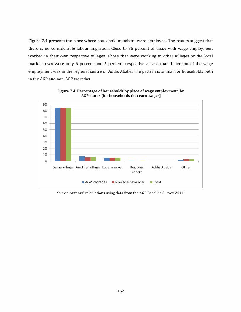
162
Figure 7.4 presents the place where household members were employed. The results suggest that
there is no considerable labour migration. Close to 85 percent of those with wage employment
worked in their own respective villages. Those that were working in other villages or the local
market town were only 6 percent and 5 percent, respectively. Less than 1 percent of the wage
employment was in the regional centre or Addis Ababa. The pattern is similar for households both
in the AGP and non-AGP woredas.
Figure 7.4. Percentage of households by place of wage employment, by AGP status [for households that earn wages]
Source: Authors’ calculations using data from the AGP Baseline Survey 2011.

163
Nonfarm Business Activities
As presented in Figure 7.5 below, the most common type of nonfarm business activity households
participate in is selling traditional food/liquor. Out of those households who indicated engagement
in any nonfarm business, 29 percent were in a business of selling traditional food or drinks. The
next common business activity is grain trade with 18 percent participation, followed by handicraft
(14 percent) and livestock trade (12 percent). Weaving/spinning, milling, selling firewood/dung,
and transport are activities carried out by a total of 7 percent of the households. In terms of
difference between AGP and non-AGP woredas, the percentage of households engaged in the
business of selling traditional food/liquor is higher by about 8 percent in AGP woredas while the
second considerable difference is observed in livestock trade where the percentage of households
in non-AGP woredas engaged in livestock trade is higher by close to 6 percent. Three percent more
households are involved in handicraft as a business activity in non-AGP woredas compared to AGP,
woredas; the difference for the remaining activities is much lower.
Figure 7.5. Percentage of households by nonfarm business activities and AGP status [for households that have nonfarm business activities]
Source: Authors’ calculations using data from the AGP Baseline Survey 2011.

164
The number of days households engage in nonfarm business differs by month (see Figure 7.6). Out
of those households with some sort of nonfarm business, most households indicated that they
worked on their nonfarm business the most between November and February with a peak in
January. About 23 percent indicated January to be the month when they had worked on their
nonfarm business the most days. The months in the main harvesting period were also the months
that households with nonfarm businesses were the most profitable. This could be because the
harvesting season is the period where most farm households are expected to have their highest
earnings from their farm production. During this period, the market for nonfarm businesses is
likely to be higher, since most farmers would be able to spend from their farm incomes. In contrast,
households with nonfarm businesses worked for the fewest days on their nonfarm business in June,
which is a planting season and when most of the resources of farm households are depleting.
Similarly, in terms of profitability, the period between May and August was also the time that
households reported that they were the least profitable from their businesses.
Figure 7.6. Months in which households had business activity for the most and fewest number of days (percentage of households with nonfarm business activities)
Source: Authors’ calculations using data from the AGP Baseline Survey 2011.

165
Table 7.3 presents the percentage of households who participate in different nonfarm businesses
by household characteristics. Most female headed households are engaged in selling traditional
food/liquor. The next common nonfarm activity for female headed households is grain trade
followed by handicraft. Although the most common activity for male headed households is also
selling traditional food/liquor, the percentage of households engaged in the activity is much lower
than for households with female heads. Grain trade and livestock trade are the second and third
most common activities for male headed households. Comparison between households with mature
and younger heads reveals that both types of households are mostly engaged in selling traditional
food/liquor. However, more households with young heads are engaged in livestock trade than
those with mature heads.
Table7.3. Percentage of households, by nonfarm business activities, household categories, and AGP status [for households that have nonfarm business activities]
Group Category Weaving
/spinning Mil-ling
Han-dicraft
Grain trade
Live-stock trade
Retail trade
Tran-sport
Selling firewood
/dung
Selling traditional food/liquor
Other
National
All HHs 3.7 1.3 14.1 18 12.2 10.6 0.9 1.2 29.3 18.4
Female HHHs 2.8 0.2 15.1 17.2 3.1 14.3 0.5 1.9 40.0 14.8
Male HHHs 4.0 1.7 13.7 18.3 15.6 9.2 1.0 0.9 25.3 19.7
Mature HHHs 4.7 1.6 15.5 19.2 8.0 10.1 0.9 1.4 32.2 16
Youth HHHs 2.5 1.0 12.4 16.6 17.2 11.1 1.0 0.9 25.8 21.3
AGP woredas
All HHs 3.0 2.0 10.7 13.9 8.1 12.6 2.1 1.6 35.5 19.4
Female HHHs 5.5 0.8 8.7 13.5 2.0 11.5 0.4 2.6 48.2 19.7
Male HHHs 1.7 2.6 11.6 14.0 11.1 13.1 3.0 1.1 29.2 19.2
Mature HHHs 4.8 1.3 16.8 20.2 8.6 9.0 0.8 1.2 31.7 14.7
Youth HHHs 2.6 0.9 12.5 17.5 18.5 11.4 0.4 0.8 23.3 22.2
Non-AGP woredas
All HHs 3.8 1.1 14.8 19.0 13.2 10.1 0.6 1.1 27.8 18.2
Female HHHs 2.0 0.0 16.9 18.3 3.4 15.1 0.6 1.7 37.6 13.4
Male HHHs 4.4 1.5 14.1 19.2 16.5 8.4 0.6 0.8 24.5 19.8
Mature HHHs 4.8 1.3 16.8 20.2 8.6 9.0 0.8 1.2 31.7 14.7
Youth HHHs 2.6 0.9 12.5 17.5 18.5 11.4 0.4 0.8 23.3 22.2
Source: Authors’ calculations using data from the AGP Baseline Survey 2011. Note: ‘HHHs’ and ‘HHs’ stand respectively for ‘Headed households’ and ‘Households’. The percentage of households could sum up more than 100 percent since households can be engaged in more than one nonfarm business activities.

166
Table 7.4 shows where households with business activities sell their output or service. Forty three
percent of the households sold their product or services within the village. The second most
common place for selling their output is in their respective local markets. Only 1.7 percent of the
households had the regional centre as their markets while those who provided to the Addis Ababa
market were only 0.1 percent. Looking into the different characteristics of households, more than
half of the female headed households had their own village as a market for their products while the
major markets for male headed households were the local markets. A slightly higher percentage of
male headed households sold their products in another village and regional centres. In comparing
young and mature heads of households, 45 percent of the mature headed households sold their
products in the same village - their main market - while 42 percent of the young headed households
did so. The main markets for young headed households were the local markets. The major markets
for non-AGP woredas were local markets while more than half of the households in the AGP
woredas sold their outputs in the same village.
Table7.4. Market for selling products/services of nonfarm businesses, by household categories and AGP status [for households that have nonfarm business activities]
Group Category
Same village
Another village
Local market
Regional centre
Addis Ababa Other
National
All HHs 43.5 7.3 41.6 1.7 0.1 5.8
Female HHHs 51.8 6.8 36.5 0.9 0.1 4.0
Male HHHs 40.3 7.4 43.5 2.1 0.2 6.5
Mature HHHs 44.9 6.9 40.1 2.6 0.2 5.3
Youth HHHs 41.7 7.7 43.5 0.7 0.0 6.4
AGP woredas
All HHs 52.4 6.0 36.4 1.4 0.2 3.6
Female HHHs 59.8 5.8 32.0 0.7 0.2 1.6
Male HHHs 48.5 6.0 38.7 1.8 0.2 4.7
Mature HHHs 51.1 5.3 38.3 1.4 0.4 3.5
Youth HHHs 54.2 6.8 33.9 1.4 0.0 3.7
Non-AGP woredas
All HHs 41.5 7.6 42.8 1.8 0.1 6.3
Female HHHs 49.4 7.1 37.9 1.0 0.0 4.7
Male HHHs 38.7 7.7 44.5 2.1 0.1 6.9
Mature HHHs 43.5 7.3 40.5 2.8 0.2 5.8
Youth HHHs 39.0 7.9 45.5 0.6 0.0 7.0
Source: Authors’ calculations using data from the AGP Baseline Survey 2011. Note: ‘HHHs’ and ‘HHs’ stand respectively for ‘Headed households’ and ‘Households’.

167
Technical Support and Credit for Nonfarm Businesses
Thirteen percent of the households who have reported to have a nonfarm business have received
some sort of technical assistance (Table7.5). The difference between male and female headed
households who have received assistance is only about 1 percent. Two percent more mature
headed households have received technical support compared to younger headed households.
Fourteen percent of households in non-AGP woredas have received technical support compared to
10 percent in AGP woredas.
Table7.5. Percentage of households who received technical assistance or credit for their nonfarm business activities, by household categories and
AGP status [for households that have nonfarm business activities]
Group Category Any technical support Borrowed
money
National
All households 13.4 18.6
Female household heads 12.8 16.6
Male household heads 13.6 19.4
Mature household heads 14.4 17.1
Youth household heads 12.3 20.5
AGP woredas
All households 10.2 17.0
Female household heads 6.4 15.7
Male household heads 12.1 17.7
Mature household heads 10.2 16.3
Youth household heads 10.2 18.0
Non-AGP woredas
All households 14.3 19.1
Female household heads 15.3 16.9
Male household heads 14.0 19.8
Mature household heads 15.6 17.4
Youth household heads 12.8 21.1
Source: Authors’ calculations using data from the AGP Baseline Survey 2011.
Out of all households who participate in nonfarm business activities, 18.6 percent have borrowed
money to finance their businesses. More male headed households have borrowed money compared
to female headed households. The percentage of households who have taken credit is 3 percent
higher for households with younger heads compared to those with mature heads. In comparing
households in AGP and non-AGP woredas, 19 percent of households in non-AGP woredas had
borrowed some money compared to 17 percent in AGP woredas.

168
For those who have indicated that they have received some sort of technical or financial assistance,
a question was asked from where they obtained such assistance. Figure 7.7 summarizes the source
of technical support and credit for the business. Most of the technical assistance for nonfarm
businesses was received from relatives and friends (70 percent of all assistance). Cooperatives gave
technical support to 8 percent of the households while the role of NGOs is only 5 percent. In terms
of credit, from the 18 percent of the households who have indicated to have received credit, the
major credit providers were again relatives and friends accounting for 50 percent of the credit. The
second most common source of credit, for those who received credit for their businesses, is micro-
credit institutions followed by cooperatives with 16 and 15 percent contribution, respectively.
Figure 7.7. Source of technical assistance and credit
Source: Authors’ calculations using data from the AGP Baseline Survey 2011.

169
Figure 7.8 compares between AGP and non-AGP woredas the sources of technical support or credit
indicated by the households. Relatives and friends are the most common sources of technical
support for households in both AGP and non-AGP woredas. The percentage of households who have
received technical support from cooperatives is 5 percent higher in AGP woredas compared to non-
AGP woredas. Not much difference is observed when considering the remaining sources of
technical support. In terms of the source of credit, the primary source of credit for households in
AGP woredas is micro-credit institutions (35 percent of the credit), while for households in non-
AGP woredas micro-credit institutions came only at the fourth place ( providing only 12 percent of
the credit). For households in non-AGP woredas friends and relatives are the primary source of
credit. The percentage of households that have received credit from NGO’s is also 3.7 percent higher
in AGP woredas than in non-AGP woredas.
Figure 7.8. Source of technical assistance and credit (percentage of households with nonfarm business activities receiving assistance/credit), by AGP status
Source: Authors’ calculations using data from the AGP Baseline Survey 2011.
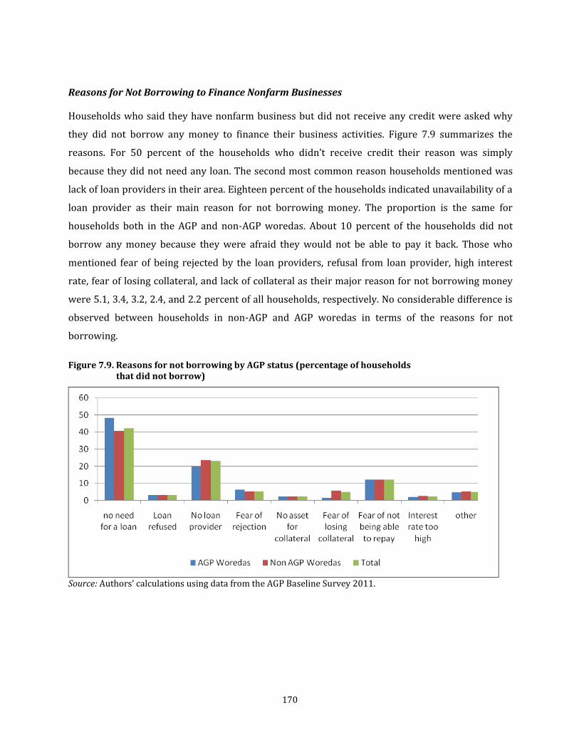
170
Reasons for Not Borrowing to Finance Nonfarm Businesses
Households who said they have nonfarm business but did not receive any credit were asked why
they did not borrow any money to finance their business activities. Figure 7.9 summarizes the
reasons. For 50 percent of the households who didn’t receive credit their reason was simply
because they did not need any loan. The second most common reason households mentioned was
lack of loan providers in their area. Eighteen percent of the households indicated unavailability of a
loan provider as their main reason for not borrowing money. The proportion is the same for
households both in the AGP and non-AGP woredas. About 10 percent of the households did not
borrow any money because they were afraid they would not be able to pay it back. Those who
mentioned fear of being rejected by the loan providers, refusal from loan provider, high interest
rate, fear of losing collateral, and lack of collateral as their major reason for not borrowing money
were 5.1, 3.4, 3.2, 2.4, and 2.2 percent of all households, respectively. No considerable difference is
observed between households in non-AGP and AGP woredas in terms of the reasons for not
borrowing.
Figure 7.9. Reasons for not borrowing by AGP status (percentage of households that did not borrow)
Source: Authors’ calculations using data from the AGP Baseline Survey 2011.

171
As presented in Table 7.6., the reason provided by households for not borrowing to finance their
nonfarm businesses differs by the household characteristics. A slightly higher percentage (2.4
percent difference) of male headed households indicated that they did not have any need for a loan
compared to female headed households. The proportion of female headed households who did not
take any loan due to fear of not being able to repay is 7 percent higher than for male headed
households. On the other hand, more male headed households reported unavailability of loan
provider as their major reason for not borrowing. In terms of comparing young and mature headed
households, fewer younger headed households reported fear of not being able to repay as their
major reason. There are more pronounced differences in the gender and age categories between
AGP and non-AGP woredas.
Table 7.6. Reason for not borrowing to finance nonfarm business (percentage of households that not borrowed), by household categories and AGP status
Group Category No need
for a loan Loan
refused No loan
provider Fear of
rejection
No asset for
collateral
Fear of losing
collateral
Fear of not being
able to repay
Interest rate too
high Other
National
All HHs 42.2 3.1 22.9 5.3 2.3 4.9 12.0 2.3 5.0
Female HHHs 41.9 3.5 16.5 5.5 3.3 4.3 17.1 2.9 5.0
Male HHHs 42.3 3.0 25.3 5.2 1.9 5.2 10.1 2.1 5.0
Mature HHHs 41.4 3.4 24.0 4.6 2.4 4.4 12.9 2.3 4.6
Youth HHHs 43.1 2.8 21.6 6.1 2.1 5.6 10.9 2.4 5.5
AGP woredas
All HHs 48.4 3.1 19.7 6.3 2.3 1.5 12.0 2.1 4.7
Female HHHs 44.0 2.6 18.4 8.5 3.3 2.1 13.9 1.3 5.8
Male HHHs 50.6 3.3 20.4 5.1 1.8 1.2 11.0 2.4 4.2
Mature HHHs 47.5 2.7 19.1 7.0 1.8 1.4 13.4 2.2 5.0
Youth HHHs 49.4 3.6 20.5 5.4 3.0 1.7 10.2 1.9 4.4
Non-AGP woredas
All HHs 40.7 3.1 23.6 5.1 2.3 5.7 12.0 2.4 5.1
Female HHHs 41.3 3.8 16.0 4.6 3.3 4.9 18.1 3.4 4.7
Male HHHs 40.5 2.9 26.4 5.2 1.9 6.0 9.9 2.1 5.2
Mature HHHs 40.0 3.5 25.1 4.1 2.6 5.1 12.8 2.3 4.5
Youth HHHs 41.6 2.6 21.8 6.3 1.9 6.5 11.1 2.5 5.8
Source: Authors’ calculations using data from the AGP Baseline Survey 2011. Note: ‘HHHs’ and ‘HHs’ stand respectively for ‘Headed households’ and ‘Households’.

172
7.3. Summary
This chapter describes wage employment and nonfarm business activities of the households in the
four regions. Of all the household members, the head of the household takes the largest percentage
in the participation in nonfarm business. In terms of age categories, the involvement of young
household heads in nonfarm business and wage employment is higher than the matured ones.
Similar, male headed households are more engaged than female headed households. However,
female headed households involved much more in selling traditional food/liquor. It was noted in
the survey results that households with young heads are more engaged in livestock trade than
those with matured heads. Male headed households appear to have better access to markets
outside their own villages while female headed households use more often their own village as a
market place for their products. The major market for selling products/service for AGP and non-
AGP woreda was found to be the same village as they are living in.
The survey results revealed that relatives and friend account for the largest share of credit source
for the households’ nonfarm businesses. However, microcredit institutions were found to be one of
the main sources of credit for households living in AGP woredas. Households in the study area were
asked to prioritize their reason for not receiving credit and a large percentage of the households
indicated that they were not interested to take the loan followed by lack of institutions to provide
loans in their area.
173
Chapter 8: Food Security, Nutrition, and Health Outcomes
As we discussed in Chapter 6 a large proportion of the crop output households produce is
consumed at home. Consequently, households’ level of food security is heavily influenced by
households’ level of food crop production. The AGP is expected to positively affect households’ level
of food security by increasing agricultural productivity, an important component of its primary
objectives. This chapter describes different dimensions of household level food security. In the first
section we describe the primary sources of household food consumption and periods in which
households were food insecure. The AGP baseline survey collected data on dietary diversity —
another dimension of food security — which will be described in the second section. In this regard,
child growth and health is susceptible to availability and nutritional content of food; making the
latter the most vulnerable item. As part of evaluating the effect of the AGP on the latter the survey
collected data on child nutrition and health, discussed also in the second section of this chapter. In
addition, the survey collected data on health status of household members as well as on sources of
drinking water. We describe health related issues and sources of potable water in the third section.
The final section summarizes.
8.1. Household Food Security
The AGP survey indicates that most rural households in Ethiopia are subsistence farmers that
derive most of their food from their own production. Households’ level of use of own-produced food
varies during different months and agricultural seasons. In Figure 8.1 we summarize households’
primary source of food for each month of the year. The data indicate that in any given month at least
three-quarters of the households used own-produced food as their main food source. From June
through September, the major raining and planting season, were the months during which the
smallest proportion of households indicated using own-produced food as their major source.
During these months purchased food was the major source for about 19 percent of the households
while food gifts, assistance from the safety net, or other forms of food aid were the major sources
for about 4 percent. The proportion of households that indicated own-produced food as their major
source of food was the highest (ranging between 90-93 percent) during the months of November to
February. The proportion purchased or obtained through some sort of assistance was the lowest
during these months.

174
Figure 8.1. Primary source of food by month (percentage of households)
Source: Authors’ calculations using data from the AGP Baseline Survey 2011.
As shown in Table 8.1 below, the proportion of households reporting own produce as major food
source is the highest in the month of December, with almost 93 percent of the households using
own production as their primary food source. This was followed by the months of January (92
percent) and November and February (90 percent). On the other hand, a considerable proportion of
the households purchased food from the market in the remaining months; from March to October
more than 10 percent of the households reported food purchased from the market as their major
food source. Similarly, a larger proportion of households are depending on gifts, safety net, and
other food aid as their primary source of food during March–October, compared to the period
November–February.
The general pattern observed is that the proportion of households which satisfy their food
requirement from own production is the largest during and after harvest season while a
considerable proportion rely on other sources in the other months. Some households are more
dependent on food aid and other programs than others. For instance a higher proportion of female
headed households indicated gift, safety net, or food aid as their major source of food in all months
of the year compared to their male counterparts. Similarly, a slightly higher proportion of female
headed households also indicated purchased food from the market as their major source of food
consumption. However, also in these two cases the proportion is smaller during and after the
harvest season.
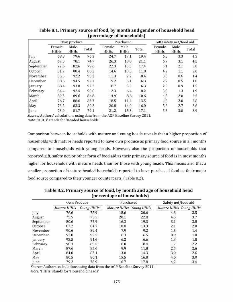
175
Table 8.1. Primary source of food, by month and gender of household head (percentage of households)
Own produce
Purchased
Gift/safety net/food aid
Female HHHs
Male HHHs
Total
Female HHHs
Male HHHs
Total
Female HHHs
Male HHHs
Total
July 68.8 79.6 76.3
24.7 17.1 19.4
6.5 3.3 4.3
August 67.0 78.1 74.7
26.3 18.8 21.1
6.7 3.1 4.2
September 72.6 82.6 79.6
22.3 15.3 17.4
5.1 2.1 3.0
October 81.2 88.4 86.2
14.6 10.5 11.8
4.2 1.1 2.0
November 85.5 92.2 90.2
11.3 7.2 8.4
3.3 0.6 1.4
December 88.6 94.5 92.7
9.2 5.1 6.3
2.2 0.5 1.0
January 88.4 93.8 92.2
8.7 5.3 6.3
2.9 0.9 1.5
February 84.4 92.4 90.0
12.3 6.4 8.2
3.3 1.3 1.9
March 80.5 89.6 86.8
14.9 8.8 10.6
4.8 2.0 2.5
April 76.7 86.6 83.7
18.5 11.4 13.5
4.8 2.0 2.8
May 73.5 83.3 80.3
20.8 14.0 16.0
5.8 2.7 3.6
June 73.0 81.7 79.1 21.2 15.3 17.1 5.8 3.0 3.9
Source: Authors’ calculations using data from the AGP Baseline Survey 2011. Note: ‘HHHs’ stands for ‘Headed households’
Comparison between households with mature and young heads reveals that a higher proportion of
households with mature heads reported to have own produce as primary food source in all months
compared to households with young heads. However, also the proportion of households that
reported gift, safety net, or other form of food aid as their primary source of food is in most months
higher for households with mature heads than for those with young heads. This means also that a
smaller proportion of mature headed households reported to have purchased food as their major
food source compared to their younger counterparts. (Table 8.2).
Table 8.2. Primary source of food, by month and age of household head (percentage of households)
Own Produce Purchased Safety net/food aid
Mature HHHs Young HHHs Mature HHHs Young HHHs Mature HHHs Young HHHs
July 76.6 75.9 18.6 20.6 4.8 3.5 August 75.5 73.5 20.1 22.8 4.5 3.7 September 80.6 77.9 16.3 19.3 3.1 2.8 October 87.2 84.7 10.8 13.3 2.1 2.0 November 90.6 89.4 7.9 9.2 1.5 1.4 December 92.8 92.5 6.3 6.5 0.9 1.0 January 92.5 91.6 6.2 6.6 1.3 1.8 February 90.3 89.5 8.0 8.4 1.7 2.2 March 87.6 85.6 9.9 11.8 2.5 2.6 April 84.0 83.1 13.0 14.3 3.0 2.6 May 80.5 80.1 15.5 16.8 4.0 3.0 June 79.2 78.9 16.7 17.8 4.2 3.4
Source: Authors’ calculations using data from the AGP Baseline Survey 2011. Note: ‘HHHs’ stands for ‘Household heads’

176
A similar comparison of households in AGP and non-AGP woredas reveals that a slightly smaller
proportion of households in non-AGP woredas rely on own production (Figure 8.2). In an average
month, 88 percent of the households in AGP woredas indicated own production as their primary
source of food while the proportion was 83 percent for households in the non-AGP woredas.
Throughout the year, an average of about 3 percent of the households in the non-AGP woredas
primarily relied on food from gifts, safety nets, or other food aid while this proportion was slightly
lower (2 percent) in AGP woredas.
Figure 8.2. Primary source of food by AGP status (100%=all households)
Source: Authors’ calculations using data from the AGP Baseline Survey 2011.
The length of period in which households experienced food shortage or were food insecure is
another measure of households’ level of food security. As shown in Figure 8.3 below, households
reported that they were food insecure for an average of 1.2 months in the one year period before
the survey. There was a difference of half a month between the periods in which male and female
headed households were food insecure. The number of months that female headed households
were food insecure was 1.5 months while it was only a month for male headed households. There is
a very slight difference between households with mature and young heads. When comparing
households in AGP woredas with those in the non-AGP woredas, we find a difference in food
security as large as the one observed between male and female headed households is observed.
Households in the AGP woredas were food insecure for an average of 0.9 months while those in the
non-AGP woredas were food insecure for 1.3 months.

177
Figure 8.3. Average number of months household was food insecure, by household categories and AGP status
Source: Authors’ calculations using data from the AGP Baseline Survey 2011. Note: ‘HHHs’ and ‘HHs’ stand respectively for ‘Household heads’ and ‘Households’.
8.2. Household Diet, and Child Nutrition and Feeding Practices
Household Diet
Household’ dietary diversity, defined as the number of food groups consumed by a household over
a given period, is another measure used to indicate the food security level of households (Hoddinott
and Yohannes, 2002). A varied diet is associated with an improved anthropometric status of
children and a lower mortality risk from different diseases (ibid.). In this survey households were
asked if they have consumed a list of food items over the past 7 days of the survey. These food items
were aggregated to form 10 major food groups17 from which the number of different food groups
consumed is calculated. The results indicate that households on average have a dietary diversity
score of 4.6. This implies that, on average, households consume about 4.6 types of food groups.
However, differences are observed among different households. Figure 8.4 presents the average
diversity score by different characteristics of household heads. Male headed households have a
higher average dietary diversity score relative to female headed households. Households with
young heads have a slightly higher dietary diversity score compared to those with mature heads.
17
The following food groups were used to create the Household Dietary Diversity Score: cereals, roots, vegetables, fruits,
meat, eggs, pulses, milk and milk products, sugar, and coffee.

178
Comparing AGP and non-AGP woredas, households in AGP woredas have a higher diversity score
compared to those in non-AGP woredas.
Figure 8.4. Household dietary diversity score, by household category and AGP status
Source: Authors’ calculations using data from the AGP Baseline Survey 2011. Note: ‘HHHs’ stands for ‘Household heads’.
Infant and Child Feeding Practices
For children under the age of 6 months breast feeding is both sufficient and beneficial for nutrition;
additional sources of feeding are discouraged since it may expose new-born infants to illness (CSA,
2011). At a later age, however, supplementary liquids and other solid foods are required for
children’s nourishment. The AGP baseline survey collected data on households’ feeding practices of
infants and children under the age of two. Information on breast feeding status is collected for each
household for a 24 hour period before the date of data collection. Moreover, data were collected on
whether the child consumed other food categories in the last 7 days. As presented in Table 8.3, 93
percent of the infants under the age of 2 months are exclusively breast fed. As the age of the infants
increases, it can be clearly seen that the percentage of infants who take supplementary food also
increases. Only 28 percent of infants under the age of 6 months are given complementary food in
addition to breast feeding while it is 50 percent for those infants between six and nine months. The
percentage of infants who are not breastfed increases with age reaching 24 percent for children
between 20 and 24 months.

179
Table 8.3. Child feeding practices by age (100%=all children in particular age group)
Months Not
breastfeeding Exclusively breastfed
Breast feeding and consuming
plain water only
Breast feeding and
liquid/juices
Breast feeding and other milk
Breast feeding and complementary
food
<2 7.4 92.6 0.0 0.0 0.0 0.0
2-3 0.0 90.8 8.4 0.0 0.0 0.8
4-5 1.7 21.2 11.6 2.1 15.0 48.4
6-7 2.8 23.8 17.6 7.9 8.0 39.8
8-9 3.8 3.4 9.4 8.1 14.3 61.0
10-11 1.4 6.7 10.7 6.1 8.9 66.2
12-15 3.1 2.8 4.6 0.5 3.0 86.1
16-19 5.5 3.4 3.1 1.1 4.5 82.4
20-24 24.4 4.0 6.1 1.0 0.5 64.0
<6 1.6 50.9 9.5 1.2 8.6 28.2
6-9 3.3 14.1 13.7 8.0 11.0 49.9
Source: Authors’ calculations using data from the AGP Baseline Survey 2011. Notes: The classification used for the feeding practices is produced similar to the presentation in the CSA EDHS (Ethiopian Demographic and Health surveys) (2011) preliminary report under the section "Infant and Child feeding practices" page 18.
As shown in Table 8.4, all infants under two months old were breast fed in the non-AGP woredas
while the proportion was lower at around 86 percent, for those in the AGP woredas. The gap is even
higher for children between the ages of two and three months with 100 percent of the infants in
non-AGP woredas exclusively breastfed relative to 58 percent in AGP woredas. A higher proportion
of children in AGP woredas (39 percent) appear to take plain water supplementing breast milk. In
non-AGP woredas 63 percent of children between four and five months are given complementary
food while the proportion is about 22 percent in AGP woredas.
Considering children under 6 months, the proportion of children who are exclusively breast fed is
1.2 percent higher in the non-AGP woredas than in the AGP woredas. However, the difference is
more substantial when considering children who are given in addition plain water, liquids/juices,
or other milk, with the proportion in non-AGP woredas being 7.8, 3.9, and 4.4 percent higher,
respectively, than the corresponding proportion in AGP woredas.
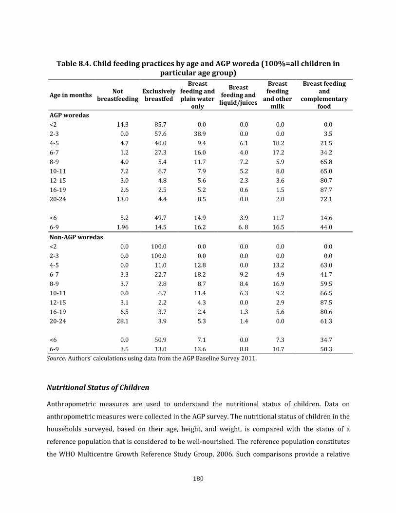
180
Table 8.4. Child feeding practices by age and AGP woreda (100%=all children in particular age group)
Age in months Not
breastfeeding Exclusively breastfed
Breast feeding and plain water
only
Breast feeding and
liquid/juices
Breast feeding
and other milk
Breast feeding and
complementary food
AGP woredas
<2 14.3 85.7 0.0 0.0 0.0 0.0
2-3 0.0 57.6 38.9 0.0 0.0 3.5
4-5 4.7 40.0 9.4 6.1 18.2 21.5
6-7 1.2 27.3 16.0 4.0 17.2 34.2
8-9 4.0 5.4 11.7 7.2 5.9 65.8
10-11 7.2 6.7 7.9 5.2 8.0 65.0
12-15 3.0 4.8 5.6 2.3 3.6 80.7
16-19 2.6 2.5 5.2 0.6 1.5 87.7
20-24 13.0 4.4 8.5 0.0 2.0 72.1
<6 5.2 49.7 14.9 3.9 11.7 14.6
6-9 1.96 14.5 16.2 6. 8 16.5 44.0
Non-AGP woredas
<2 0.0 100.0 0.0 0.0 0.0 0.0
2-3 0.0 100.0 0.0 0.0 0.0 0.0
4-5 0.0 11.0 12.8 0.0 13.2 63.0
6-7 3.3 22.7 18.2 9.2 4.9 41.7
8-9 3.7 2.8 8.7 8.4 16.9 59.5
10-11 0.0 6.7 11.4 6.3 9.2 66.5
12-15 3.1 2.2 4.3 0.0 2.9 87.5
16-19 6.5 3.7 2.4 1.3 5.6 80.6
20-24 28.1 3.9 5.3 1.4 0.0 61.3
<6 0.0 50.9 7.1 0.0 7.3 34.7
6-9 3.5 13.0 13.6 8.8 10.7 50.3
Source: Authors’ calculations using data from the AGP Baseline Survey 2011.
Nutritional Status of Children
Anthropometric measures are used to understand the nutritional status of children. Data on
anthropometric measures were collected in the AGP survey. The nutritional status of children in the
households surveyed, based on their age, height, and weight, is compared with the status of a
reference population that is considered to be well-nourished. The reference population constitutes
the WHO Multicentre Growth Reference Study Group, 2006. Such comparisons provide a relative
181
measure of the nutritional status of children in the households surveyed. Accordingly, measures of
age-for-height, age-for-weight, and weight-for-height are used. A more than minus two standard
deviation (-2Sd) from the median of the reference population is an indication of moderate
malnourishment while a minus three standard deviation (-3Sd) is a severe case of malnourishment.
Children who have a height-for-age less than minus two standard deviations from the median of the
reference population are considered to be short for their age, a condition described as moderate
stunting. Moreover, those with less than minus three standard deviations are considered to be
severely stunted. Stunting is a cumulative indication of a long term malnourishment. In this survey,
46.2 percent of children under the age of five were found to be stunted while 26.7 percent were
severely stunted (Figure 8.5). A larger proportion of boys were stunted compared to girls; slightly
less than half of the boys under the age of five were stunted while it was 45 percent for girls. Also, 4
percent more boys were severely stunted compared to girls.
An indicator for the current nutritional status of children is weight-for-height. Depending on the
severity of the incidence, a child that is too thin for his/her height is referred to as wasted or
severely wasted. The data in this survey indicates that 12 percent of the children were wasted while
5.7 percent were severely wasted. As in the case of stunting, more boys are both moderately and
severely wasted as compared to girls. However the difference between boys and girls is lower in the
case of wasting than that of stunting.
Weight for age is considered as an indicator for both acute and chronic malnutrition. It measures
whether the weight of a child for his/her age is much different from a reference of a well-nourished
population. About 27 percent of the children surveyed are underweight while 10 percent are
severely underweight. Relative to girls, the proportion of boys moderately and severely
underweight is higher by 3.1 and 1.1 percentage points, respectively.
Table 8.5 compares the level of child malnourishment among different household categories. The
proportion of stunted, wasted, and underweight children is lower in female headed households,
which also perform better in all three severely malnourished versions of the measures. The
proportion of malnourished children is higher for households with young heads than for those with
mature heads, with the exception of proportion of children that are wasted being larger in mature
headed households.
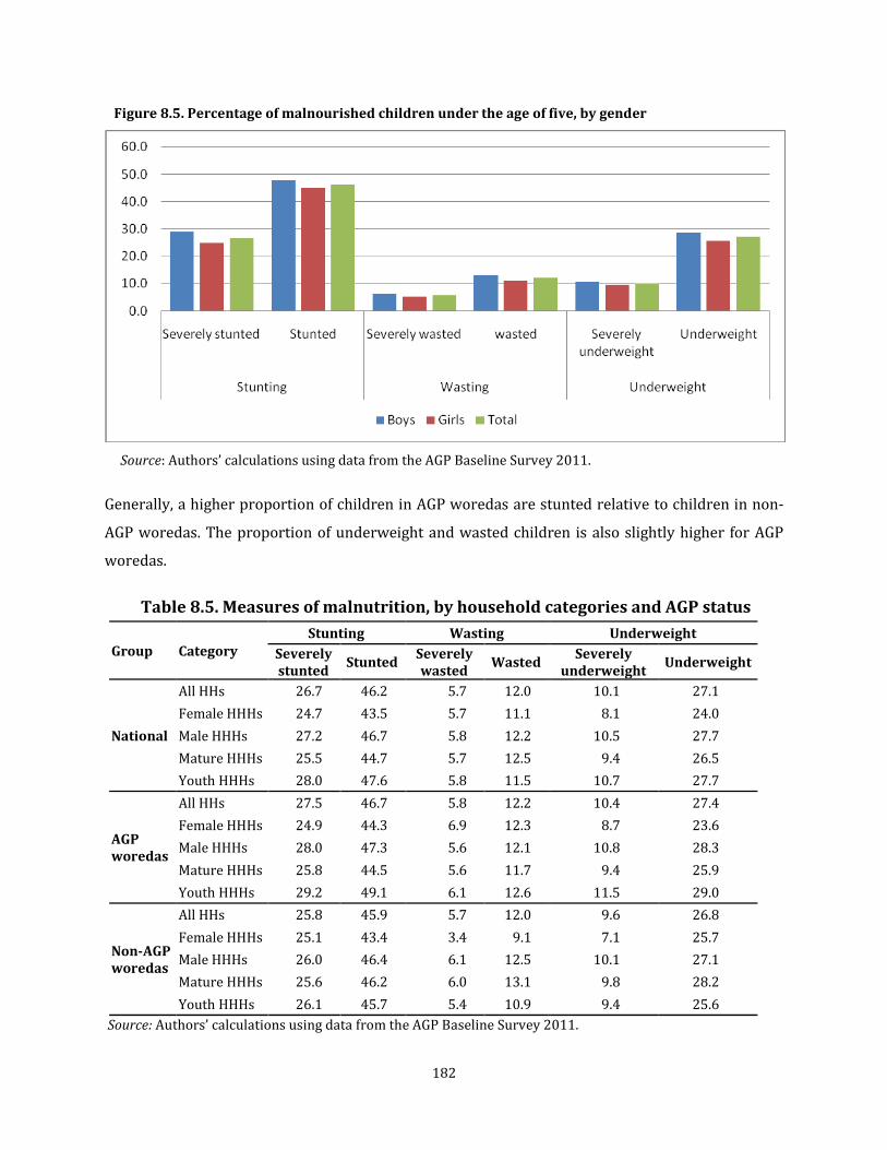
182
Figure 8.5. Percentage of malnourished children under the age of five, by gender
Source: Authors’ calculations using data from the AGP Baseline Survey 2011.
Generally, a higher proportion of children in AGP woredas are stunted relative to children in non-
AGP woredas. The proportion of underweight and wasted children is also slightly higher for AGP
woredas.
Table 8.5. Measures of malnutrition, by household categories and AGP status
Group Category Stunting Wasting Underweight
Severely stunted
Stunted Severely wasted
Wasted Severely
underweight Underweight
National
All HHs 26.7 46.2 5.7 12.0 10.1 27.1
Female HHHs 24.7 43.5 5.7 11.1 8.1 24.0
Male HHHs 27.2 46.7 5.8 12.2 10.5 27.7
Mature HHHs 25.5 44.7 5.7 12.5 9.4 26.5
Youth HHHs 28.0 47.6 5.8 11.5 10.7 27.7
AGP woredas
All HHs 27.5 46.7 5.8 12.2 10.4 27.4
Female HHHs 24.9 44.3 6.9 12.3 8.7 23.6
Male HHHs 28.0 47.3 5.6 12.1 10.8 28.3
Mature HHHs 25.8 44.5 5.6 11.7 9.4 25.9
Youth HHHs 29.2 49.1 6.1 12.6 11.5 29.0
Non-AGP woredas
All HHs 25.8 45.9 5.7 12.0 9.6 26.8
Female HHHs 25.1 43.4 3.4 9.1 7.1 25.7
Male HHHs 26.0 46.4 6.1 12.5 10.1 27.1
Mature HHHs 25.6 46.2 6.0 13.1 9.8 28.2
Youth HHHs 26.1 45.7 5.4 10.9 9.4 25.6
Source: Authors’ calculations using data from the AGP Baseline Survey 2011.
183
Note: ‘HHHs’ and ‘HHs’ stand respectively for ‘Headed households’ and ‘Households’
8.3. Child and Adult Health
This section describes the health status of household members and households’ access to safe
drinking water. In the first subsection we discuss about the health status of children under 5 years
of age while the second section deals with members 15 years and older. Due to the contribution of
safe drinking water to a healthy diet and the negative effects of waterborne diseases that could
result from inaccessibility of safe drinking water we also describe households’ access to the latter in
this section.
Child Health
According to WHO (2011) acute respiratory infections and diarrhoea are among the leading causes
of death in children under age of 5 years in developing countries. The AGP baseline survey asked
households if children under the age of two years were sick of fever, coughing/cold, had breathing
problems or diarrhoea in the two weeks before the survey. Figure 8.6 presents the prevalence of
common child diseases by AGP status. Thirty seven percent of the children were reported to have
been coughing while about 15 percent had some sort of a breathing problem. About 32 and 25
percent of the children had fever and diarrhoea, respectively. A higher proportion of children in
non-AGP woredas had some sort of breathing problems (3.5 percent more), coughing (3.1 percent
more), and fever (2.9 percent more) compared the children in AGP woredas, while diarrhoea was
more prevalent in AGP woredas (1.0 percent more).

184
Figure 8.6. Percentage of children under the age of five with common diseases, by AGP status
Source: Authors’ calculations using data from the AGP Baseline Survey 2011.
The difference in the prevalence of common child diseases among different household groups is
given in Table 8.6. The proportion of children affected by fever, respiratory infections, and
diarrhoea is slightly higher in female headed households than in male headed households. A higher
proportion of children in households with mature heads were affected by fever, breathing problem,
and diarrhoea relative to households with young heads while the reverse is true for coughing.
Table 8.6. Percentage of children under the age of five with common diseases, by household categories and AGP status
Group Category Fever Coughing Breathing problem Diarrhoea
National
All HHs 32.2 36.7 15.0 25.2
Female HHHs 33.5 38.3 15.0 24.6
Male HHHs 32.0 36.5 15.0 25.3
Mature HHHs 34.5 34.9 16.5 25.8
Youth HHHs 30.7 38.0 14.0 24.7
AGP woredas
All HHs 30.1 34.6 12.5 26.2
Female HHHs 37.9 43.2 17.6 31.2
Male HHHs 28.8 33.1 11.6 25.3
Mature HHHs 32.1 32.4 15.0 26.4
Youth HHHs 28.8 36.0 10.8 26.0
Non-AGP woredas
All HHs 33.1 37.6 16.0 24.8
Female HHHs 31.8 36.4 14.0 22.1
Male HHHs 33.3 37.8 16.3 25.2
Mature HHHs 35.5 35.8 17.1 25.5
Youth HHHs 31.4 38.8 15.2 24.3 Source: Authors’ calculations using data from the AGP Baseline Survey 2011. Note: ‘HHHs’ and ‘HHs’ stand respectively for ‘Headed households’ and ‘Households’

185
Adult Health
Respondents were asked about the health status of the adult household members (15 years or
older). This mainly focused on whether such household members were not able to participate in
any work, inside or outside of the household, due to any kind of hearing or vision problems or due
to some sort of accident or injury. Figures 8.7.a and 8.7.b present the proportion of households that
reported they had one or more such members. About 4 percent reported that at least one member
of the household is unable to work due to hearing or vision problems. Relatively more (5.2 percent)
female headed households have at least one member with hearing/vision problem compared to
male headed households (3.3 percent). There are more households with mature heads with at least
one member with hearing or vision problems relative to those with young heads. More households
in non-AGP woredas (4.3 percent) have members unable to work due to hearing or vision problems
when compared with those in AGP woredas (2.7 percent). A more or less similar pattern is
observed in the case of households having members with disabilities due to accidents or injury.
Figure 8.7.a. Percentage of households with at least one member having a hearing or vision problem, by household categories and AGP status
Source: Authors’ calculations using data from the AGP Baseline Survey 2011. Note: ‘HHHs’ and ‘HHs’ stand respectively for ‘Headed households‘ and ‘Households’

186
Figure 8.7.b. Percentage of households with at least one member having a disability caused by injury or accident, by household categories and AGP status
Source: Authors’ calculations using data from the AGP Baseline Survey 2011. Note: ‘HHHs’ and ‘HHs’ stand respectively for ‘Headed households’ and ‘Households’
Source of Water
Access to safe drinking water is limited in most rural areas of Ethiopia. As a result of this,
households use water sources that are not safe. In this survey respondents were asked to indicate
where they get the water they use for drinking and other purposes. The sources were then
categorized into safe water sources or otherwise. Households are said to have access to safe
drinking water sources if they obtain their drinking water primarily from protected wells,
private/public standpipes, or rain water collection while sources such as lakes, rivers, or
unprotected wells or springs are considered as unsafe. Table 8.7 presents the proportion of
households with access to safe drinking water by household characteristics. Only less than half of
the households surveyed (46 percent) have access to safe drinking water. Although male and
mature headed households have slightly better access to safe water compared to their respective
counterparts, the proportions are close to each other. The difference between non-AGP and AGP
woredas stands at 8.4 percentage points, with more households having access to safe water in non-
AGP woredas than in AGP woredas.
Slightly more than 44 percent of the households use the same water source for drinking as well as
for other purposes and this holds true among both female and male headed households. Slightly
more households with younger heads use the same water source for drinking and other purposes at
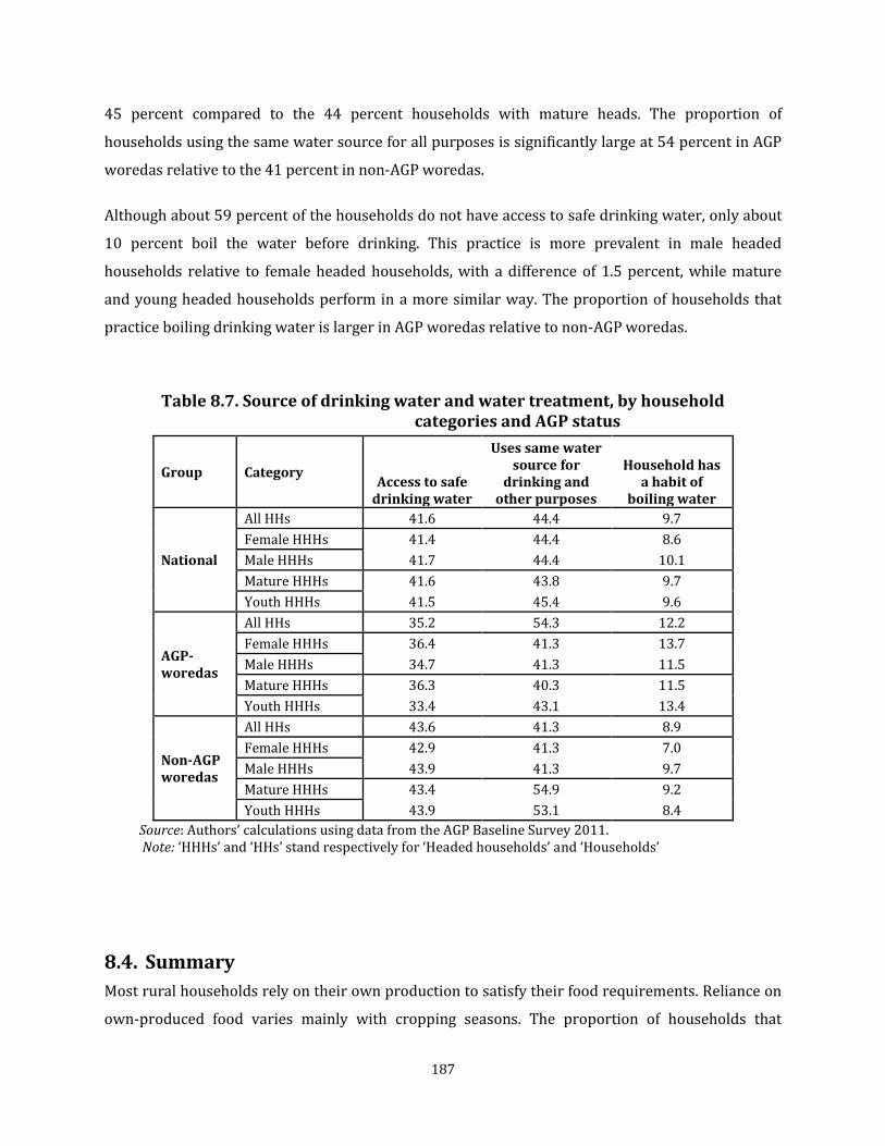
187
45 percent compared to the 44 percent households with mature heads. The proportion of
households using the same water source for all purposes is significantly large at 54 percent in AGP
woredas relative to the 41 percent in non-AGP woredas.
Although about 59 percent of the households do not have access to safe drinking water, only about
10 percent boil the water before drinking. This practice is more prevalent in male headed
households relative to female headed households, with a difference of 1.5 percent, while mature
and young headed households perform in a more similar way. The proportion of households that
practice boiling drinking water is larger in AGP woredas relative to non-AGP woredas.
Table 8.7. Source of drinking water and water treatment, by household categories and AGP status
Group Category Access to safe
drinking water
Uses same water source for
drinking and other purposes
Household has a habit of
boiling water
National
All HHs 41.6 44.4 9.7
Female HHHs 41.4 44.4 8.6
Male HHHs 41.7 44.4 10.1
Mature HHHs 41.6 43.8 9.7
Youth HHHs 41.5 45.4 9.6
AGP- woredas
All HHs 35.2 54.3 12.2
Female HHHs 36.4 41.3 13.7
Male HHHs 34.7 41.3 11.5
Mature HHHs 36.3 40.3 11.5
Youth HHHs 33.4 43.1 13.4
Non-AGP woredas
All HHs 43.6 41.3 8.9
Female HHHs 42.9 41.3 7.0
Male HHHs 43.9 41.3 9.7
Mature HHHs 43.4 54.9 9.2
Youth HHHs 43.9 53.1 8.4
Source: Authors’ calculations using data from the AGP Baseline Survey 2011. Note: ‘HHHs’ and ‘HHs’ stand respectively for ‘Headed households’ and ‘Households’
8.4. Summary
Most rural households rely on their own production to satisfy their food requirements. Reliance on
own-produced food varies mainly with cropping seasons. The proportion of households that

188
indicated own-produced food as their major food source is largest during and after harvest and is
smallest during the raining and planting months of the main agricultural season. During these latter
months a considerable proportion of households had to purchase food or obtained it from other
sources to cover the food deficit. Moreover, the data indicate that an average household was food
insecure for 1.2 months during the year. Male headed and households in AGP woredas performed
relatively better.
The data also indicate that the items household members consumed were less than half as diverse
as required for a healthy diet. Although dietary diversity varied among the different categories and
woredas, the variation was small. Long- and short-term nutritional status of children under the age
of 5 was examined using anthropometric measures collected in the survey. The results indicate a
prevalence of severe stunting, wasting, and underweight in 27, 6, and 10 percent of the children.
The proportion with moderate stunting, wasting, and underweight was 46, 12, and 27 percent,
respectively. Children in households with female and mature heads and those in non-AGP woredas
performed better in all or most measures. Diarrhoea, coughing, fever, and breathing problems
affected 25, 37, 32, and 15 percent of the children in the 2 weeks prior to the survey.
Less than half of the households have access to safe drinking water and more than 40 percent use
the same water for drinking and other purposes. While there were differences among household
categories in access to safe water the differences were small. Although about 58 percent of the
households do not have access to safe drinking water, less than 10 percent boil the water they
drink. This practice is more prevalent in male and mature headed households.
189
References
Central Statistical Agency (CSA) [Ethiopia] and ICF Macro. 2011. Ethiopia Demographic and
Health survey 2011. Preliminary Report. Addis Ababa, Ethiopia and Calverton, Maryland,
USA: CSA and ICF International.
CSA (Central Statistical Agency). 2008. Agricultural sample survey 2007/08. Volume II. Report
on livestock and livestock characteristics (private peasant holdings). CSA, Addis Ababa,
Ethiopia.
Hoddinott, John and Yisehac Yohannes. 2002. Dietary Diversity as a Household Food Security
Indicatory. Washington DC: Food and Nutrition Technical Assistance Project Academy for
Educational Development.
James, A.D., and Carles, A.B. 1996. Measuring the Productivity of Grazing and Foraging
Livestock. Agricultural Systems, Vol. 52. No2/3 pp271-291
Jones, Alicia Noelle (2002). “Density of Milk,” in The Physics Factbook™, Edited by Glenn Elert -
Written by his student, accessed at
http://hypertextbook.com/facts/2002/AliciaNoelleJones.shtml
Miller, R.C., D.L. French, and P.G. Jennings. 2007. Revitalization of the Jamaican Dairy Sector:
Evaluation of the Feasibility of Business Models for Intensive Dairy Production. Report
prepared for Annual Conference 2007, Jamaican Society for Agricultural Sciences,
September 2007. Retrieved from
http://www.jddb.gov.jm/files/Publications/models_for_intensive_dairy_production.pdf
MoARD (June, 2010). Agricultural Growth Program (AGP) - Program Implementation Mannual
(PIM) (Main Text), Ministry of Agriculture and Rural Development (MoARD), Federal
Democratic Republic of Ethiopia, Addis Ababa.
World Bank (September, 2010). Ethiopia: Agricultural Growth Project – Project Appraisal
Document (PAD), Sustainable Development Department, Agriculture and Rural
Development Unit Country Department 3, Africa Region, the World Bank.
World Health Organization (WHO) Multicentre Growth Reference Study Group. 2006. WHO
Child Growth Standards: Length/height-for-age, weight-for-age, weight-for-length,
weight-for-height and body mass index-for-age: Methods and development. Geneva: WHO.
World Health Organization (WHO). 2011. World Health Statistics. WHO. Geneva.

190
Annexes
Annex A: AGP Details Project implementation period: Start December 1, 2010; End: September 30, 2015
Expected Effectiveness Date: December 1, 2010
Expected Closing Date: September 30, 2015
Annex Table A.1.1. List of AGP woredas
Region No Zone AGP woreda Region No Zone AGP woreda
Oro
miy
a
1
North Shewa
Hidebu Habote
Am
har
a
1
West Gojam
Jabi-tehnane
2 G/Jarso 2 Bure
3 Yaya Gulele 3 Wenebrema
4
West Shewa
Dendi 4 Debube Achefer
5 Ambo 5 Semin
6 Toke Kutaye 6 Bahir-DarKetma Zuria
7
South West Shewa
Bacho (Tulu Bolo) 7
East Gojam
Dejene
8 Wenchi 8 Enmaye
9 Weliso 9 Debre Elias
10
East Shewa
Ada’a 10
Awi
Anikasha (Ankasha)
11 Liban 11 Gwangwa (Guangua)
12 Gimbichu 12 Danegela (Dangila)
13
East Wollega
Gutu Gida 13 Jawi
14 Diga 14
Semen Gondar
Taqusa
15 Wayu Tuqa 15 Metma (Metema)
16 Horo Guduru
Wollega
Guduru 16 Qura
17 Jima-Genet 17 Alefa
18 Horo 18 Debub Gondar Dera
19
Illu Aba Bora
Gechi 19
North Shewa
Efratana- Gidim
20 Bedele 20 Anitsokiya-Gemza
21 Dhedhesa 21 Qewt
22
Jimma
Goma 22 Tarma Ber
23 Gera
SNN
PR
1 Kaffa
Chena
24 Limu saqaa 2 Decha
25
Arsi
Limu-Bilbilo 3 Gurage
Enemor na ener
26 Shirka 4 Endegeng (Endegegn)
27 Munesa 5 Silte
Merab Azernet
28
West Arsi
Dodola 6 Misrak Azernet
29 Adaba 7
Sidama
Gorche (Shebedino)
30 Kofele 8 Malga (Malga)
31
Bale Zone
Sinana 9 Wondo Genet
32 Gasera 10 Dawro
Esira (Isara)
33 Agarfa 11 Konta
34 Special Welmera 12 Debub Omo
Debub Ari
Tig
ray
1
Southern
Alamata 13 Semen Ari
2 Raya/Azebo 14 Bench Maji
Debub Bench
3 Ofla 15 Sheye bench
4 Enidemhoni 16 Gedeo
Bule
5
Western
Tsegde 17 Gedeb
6 Welqayt 18 Special woredas
Yem
7 Qfta humra 19 Besketo
8 North Western Tahtaye-adiyabo
Source: World Bank (September, 2010)

191
Annex Table A.1.2. Sampled AGP-woredas Region Zone Woreda Tigray North Western Tigray Tahitay Adiyabo Tigray South Tigray Endamehone Tigray South Tigray Rya Azebo Tigray South Tigray Alamata Tigray South Tigray Ofla Tigray Western Tigray Qafta Humera Tigray Western Tigray Welqayet Tigray Western Tigray Tsegede Amhara North Gondar Metema Amhara North Gondar Alefa Amhara North Gondar Takusa Amhara South Gonder Dera Amhara North Shewa Antsokiya Gemza Amhara North Shewa Yifratana Gidim Amhara North Shewa Kewet Amhara East Gojjam Enemay Amhara East Gojjam Debere Elias Amhara East Gojjam Dejen Amhara West Gojjam Bahir Dar Zuriya Amhara West Gojjam Jebitenan Amhara West Gojjam Bure Amhara West Gojjam South Achefer Amhara Awi Dengila Amhara Awi Ankasha Guagusa Amhara Awi Guangua Amhara Awi Jawi Oromiya East Wellega Wayu Tuqa Oromiya Ilu Aba Bora Gechi Oromiya Ilu Aba Bora Bedele Zuriya Oromiya Jimma Limu Seka Oromiya Jimma Gomma Oromiya West Shewa Ambo Oromiya West Shewa Dendi Oromiya North Shewa Hidabu Abote Oromiya North Shewa Yaya Gulele Oromiya East Shewa Adea Oromiya Arsi Shirka Oromiya Arsi Limuna Bilbilo Oromiya Bale Agarfa Oromiya Bale Sinana Oromiya South West Shewa Weliso Oromiya West Arsi Kofele Oromiya West Arsi Dodola Oromiya Horo Gudru Wellega Guduru SNNPR Gurage Endegeng SNNPR Gurage Enemor na ener SNNPR Sidama Gorche SNNPR Sidama Malga SNNPR Sidama Wendo Genet SNNPR Gedeo Bule SNNPR Gedeo Gedeb SNNPR South Omo South Ari SNNPR Kefa Decha SNNPR Kefa Chena SNNPR Bench Maji Southern Bench SNNPR Bench Maji Shay Bench SNNPR YEM Yem Special SNNPR Dawuro Esira SNNPR Basketo Basketo SNNPR Konta Konta Special SNNPR Siliti Mirab Azenet

192
Annex Table A.1.3. Sampled Non-AGP woredas
Region Zone Woreda
Tigray North Western Tigray Asegede Tsimbila
Tigray Central Tigray Ahiferom
Tigray Eastern Tigray Saesi Tsadamba
Tigray South Tigray Enderta
Amhara North Gondar Dembia
Amhara South Gonder Simada
Amhara South Wolo Mekdela
Amhara South Wolo Legamibo
Amhara North Shewa Mojana Wedera
Amhara East Gojjam Enarj Enawuga
Amhara West Gojjam Dembecha
Amhara West Gojjam Gonji Kolela
Amhara Argoba Special woreda Argoba
Oromiya West Wellega Ayira
Oromiya Jimma Limu Kosa
Oromiya West Shewa Jeldu
Oromiya North Shewa Abichugna
Oromiya East Shewa Dugda
Oromiya Arsi Tiyo
Oromiya Bale Dinsho
Oromiya Qeleme Wellega Dale Wabera
Oromiya Horo Gudru Wellega Jima Rare
SNNPR Gurage Muhur NA Aklil
SNNPR Kembata Timbaro Anigacha
SNNPR Sidama Aleta Wondo
SNNPR Sidama Chire
SNNPR Wolayita Damot Gale
SNNPR South Omo Gelila
SNNPR Kefa Gesha
SNNPR Gamo Gofa Chencha
SNNPR Amaro Special Amaro Special Wereda
SNNPR Alaba Alaba

193
Annex B: Tables
Annex Table B.2.1. Descriptives statistics on household head’s age, by region and AGP status
Group Category Statistics
Mean SD Median Maximum Minimum
Tigray
All HHS 43 14.6 40 97 18
AGP woredas 42.4 14.3 40 97 18
Non-AGP woredas 44 14.9 40 86 20
Amhara
All HHS 43.6 15.4 40 98 18
AGP woredas 42.7 14.9 39 90 18
Non-AGP woredas 43.9 15.6 40 98 19
Oromiya
All HHS 42.9 15.9 40 98 16
AGP woredas 43.8 16.2 40 98 16
Non-AGP woredas 42.6 15.8 40 89 17
SNNP
All HHS 42.6 15.3 38 97 15
AGP woredas 41.3 14 38 91 15
Non-AGP woredas 42.9 15.5 39 97 15
Source: Authors’ calculations using data from the AGP Baseline Survey 2011. Notes: ‘HHs’ stands for ‘Households’. SD represents ‘Standard Deviation’.
Annex Table B.2.2. Proportion of household head’s marital status, by region and AGP status
Group Category Married,
single spouse
Single Divorced Widowed Separated
Married, more than one
spouse
Tigray
All HHS 65.5 1.7 14.8 12.9 0.6 4.6
AGP woredas 63.6 1.3 16.4 11.7 0.7 6.2
Non-AGP woredas 68.7 2.4 12.0 14.8 0.4 1.7
Amhara
All HHS 67.1 0.7 11.0 17.0 1.7 2.4
AGP woredas 67.1 0.8 11.3 15.6 1.8 3.5
Non-AGP woredas 67.2 0.7 10.9 17.5 1.7 2.0
Oromiya
All HHS 67.5 2.8 3.3 15.6 1.8 9.0
AGP woredas 66.8 2.7 4.5 18.2 1.0 6.8
Non-AGP woredas 67.7 2.8 3.0 14.7 2.1 9.7
SNNP
All HHS 72.3 3.5 1.9 14.1 0.6 7.6
AGP woredas 69.8 3.1 1.7 15.0 1.1 9.3
Non-AGP woredas 72.9 3.6 1.9 13.9 0.6 7.2
Source: Authors’ calculations using data from the AGP Baseline Survey 2011.
Note: ‘HHs’ stands for ‘Households’.

194
Annex Table B.2.3. Average household size, by region and AGP status
Group Category 1-2 3-4 5-6 7-8 9-10 11 or more
Average
Tigray
All HHS 18.5 33.6 29.0 14.9 3.7 0.4 4.6
AGP woredas 20.6 34.6 28.4 12.8 3.4 0.3 4.4
Non-AGP woredas 15.0 31.7 30.1 18.4 4.2 0.5 4.8
Amhara
All HHS 18.4 38.8 26.8 11.2 4.3 0.5 4.4
AGP woredas 18.4 37.0 27.5 13.2 3.6 0.3 4.4
Non-AGP woredas 18.4 39.3 26.6 10.6 4.6 0.5 4.4
Oromiya
All HHS 12.1 33.6 29.2 17.2 5.8 2.1 5.1
AGP woredas 14.9 34.8 28.0 15.6 5.8 0.9 4.8
Non-AGP woredas 11.2 33.2 29.6 17.7 5.7 2.5 5.1
SNNP
All HHS 12.5 30.5 34.5 17.1 4.7 0.8 5.0
AGP woredas 14.5 33.0 31.8 16.8 3.6 0.3 4.8
Non-AGP woredas 12.0 29.9 35.1 17.1 4.9 0.9 5.0
Source: Authors’ calculations using data from the AGP Baseline Survey 2011. Note: ‘HHs’ stands for ‘Households’.
Annex Table B.2.4. Percentage of households with members of different age groups, by region and AGP status
Group Category under 5 Ages 5-15
Ages 16-24
Ages 25-34
Ages 35-59
Ages 60 or more
Average age (all
members)
Average age(5
years or older
Tigray
All HHS 19.4 29.3 17.0 14.0 15.6 4.7 21 24.7
AGP woredas 18.3 29.2 17.9 14.3 16.0 4.3 21 24.5
Non-AGP woredas
21.0 29.4 15.6 13.6 15.0 5.4 21 25
Amhara
All HHS 15.4 29.7 17.5 15.7 16.0 5.8 22.5 25.6
AGP woredas 16.2 29.9 17.2 15.8 15.9 4.9 21.8 24.9
Non-AGP woredas
15.1 29.6 17.5 15.6 16.0 6.0 22.7 25.8
Oromiya
All HHS 18.2 31.6 16.8 13.8 14.3 5.3 20.9 24.2
AGP woredas 16.1 32.9 17.5 13.4 14.4 5.6 21.3 24.4
Non-AGP woredas
18.8 31.2 16.6 13.9 14.3 5.2 20.7 24.2
SNNP
All HHS 18.6 33.5 13.9 14.4 15.0 4.6 20.5 24.2
AGP woredas 19.3 34.5 13.1 13.4 16.2 3.5 19.8 23.5
Non-AGP woredas
18.5 33.3 14.1 14.6 14.8 4.8 20.7 24.3
Source: Authors’ calculations using data from the AGP Baseline Survey 2011. Note: ‘HHs’ stands for ‘Households’.

195
Annex Table B.2.5. Percentage of households with children under 5 years old of different age groups, by household categories and AGP status
Group Category 0-11 months
12-23 months
24-35 months
36-47 months
48-60 months
Tigray
All HHS 19.7 19.5 16.9 23.0 20.9
AGP woredas 20.2 18.9 17.3 22.6 20.9
Non-AGP woredas 18.9 20.2 16.3 23.5 21.0
Amhara
All HHS 17.5 19.5 17.1 21.4 24.5
AGP woredas 18.7 20.5 20.2 20.5 20.1
Non-AGP woredas 17.1 19.2 16.1 21.7 25.9
Oromiya
All HHS 20.8 18.8 18.2 21.8 20.4
AGP woredas 19.6 20.3 17.3 19.6 23.3
Non-AGP woredas 21.2 18.4 18.5 22.4 19.6
SNNP
All HHS 20.7 15.8 19.7 22.1 21.7
AGP woredas 20.4 18.5 17.7 23.3 20.2
Non-AGP woredas 20.8 15.2 20.1 21.8 22.1
Source: Authors’ calculations using AGP baseline survey data. Note: ‘HHs’ stands for ‘Households’.
Annex Table B.2.6. Percentage of household heads with different education level, by region and AGP status
Group Category Illiterate Informal
education Primary
education Secondary education
Higher education
Tigray
All HHS 62.7 10.0 25.1 2.1 0.03
AGP woredas 68.0 9.3 21.3 1.4 0.04
Non-AGP woredas 53.7 11.3 31.6 3.4 -
Amhara
All HHS 64.5 18.7 15.8 0.8 0.2
AGP woredas 66.5 16.4 15.5 1.4 0.2
Non-AGP woredas 63.9 19.4 15.9 0.6 0.1
Oromiya
All HHS 45.3 13.1 37.4 3.0 1.2
AGP woredas 61.6 5.0 30.1 3.0 0.4
Non-AGP woredas 39.9 15.8 39.8 3.0 1.4
SNNP
All HHS 56.8 1.6 36.9 4.0 0.7
AGP woredas 63.0 1.6 32.6 2.2 0.5
Non-AGP woredas 55.4 1.6 37.9 4.4 0.8
Source: Authors’ calculations using data from the AGP Baseline Survey 2011. Note: ‘HHs’ stands for ‘Households’.

196
Annex Table B.2.7.Percentage of household heads’ occupation of by region and AGP status
Group Category Farmer or
family farm worker
Domestic work
Manual work
Trained worker
Crafts person
Self-employed
Employed in service
sector Student Other
Tigray
All HHS 89.7 5.1 1.2 - 0.2 1.0 0.4 0.1 2.3
AGP woredas 89.5 5.7 0.8 - 0.2 1.3 0.6 0.1 1.8
Non-AGP woredas 90.1 4.1 1.9 - 0.2 0.5 0.2 0.2 3.0
Amhara
All HHS 88.6 7.7 0.2 0.02 0.3 1.1 0.2 0.3 1.6
AGP woredas 90.0 5.2 0.8 0.1 0.3 1.1 0.3 0.2 2.1
Non-AGP woredas 88.2 8.5 - - 0.3 1.2 0.1 0.3 1.5
Oromiya
All HHS 90.9 4.2 0.6 0.04 0.4 0.4 0.6 0.0 2.7
AGP woredas 90.5 4.7 1.0 0.2 0.2 0.5 0.3 0.2 2.3
Non-AGP woredas 91.1 4.0 0.5 - 0.5 0.3 0.7 - 2.9
SNNP
All HHS 85.7 10.4 0.3 0.1 0.2 0.8 0.4 0.6 1.4
AGP woredas 86.0 9.2 0.7 0.1 0.5 0.8 0.7 0.7 1.2
Non-AGP woredas 85.6 10.7 0.3 0.1 0.1 0.8 0.4 0.6 1.4
Source: Authors’ calculations using data from the AGP Baseline Survey 2011. Note: ‘HHs’ stands for ‘Households’.
Annex Table B.2.8.Percentage of household heads that used different materials to construct their dwelling, by region and AGP status
Region Category
Roof Floor
Plastic sheeting
Thatched Mud/sand/stone, etc.
Corrugated metal
Earth Cow dung
mixed with soil
Concrete/stone/ cement
Tile
Tigray
All HHS 2.4 39.1 24.3 34.2 65.7 33.1 0.9 0.2
AGP woredas 2.8 53.7 11.1 32.4 61.6 38.0 0.2 0.3
Non-AGP woredas 1.6 14.0 47.1 37.2 72.8 24.8 2.2 0.2
Amhara
All HHS 2.1 40.4 - 57.5 42.2 57.5 0.3 0.03
AGP woredas 1.5 61.7 0.3 36.5 54.9 44.3 0.7 0.1
Non-AGP woredas 1.1 34.4 - 64.6 38.4 61.5 0.1 -
Oromiya
All HHS 1.5 61.3 0.3 37.0 73.9 25.6 0.3 0.1
AGP woredas 1.4 59.9 0.1 38.6 63.7 36.0 0.3 -
Non-AGP woredas 1.5 61.7 0.3 36.5 77.2 22.3 0.3 0.1
SNNP
All HHS 2.3 80.2 2.7 14.8 62.5 36.2 1.0 0.3
AGP woredas 1.3 76.0 4.7 18.1 39.6 57.7 2.2 0.6
Non-AGP woredas 2.5 81.2 2.2 14.1 67.6 31.4 0.8 0.2
Source: Authors’ calculations using data from the AGP Baseline Survey 2011.
Note: ‘HHs’ stands for ‘Households’.

197
Annex Table B.2. 9. Percentage of household heads’ asset ownership structure, by region and AGP status
Group Category Stove Sofa Bed Mobile Radio/
Television Jewelry Table/ chair
Wheel-barrow
cart Car
Tigray
All HHS 27.6 3.9 42.4 12.9 25.8 26.6 2.8 1.4 0.2
AGP woredas 28.2 4.2 46.4 10.6 21.2 21.4 3.5 1.8 0.2
Non-AGP woredas 26.7 3.4 35.6 16.9 33.6 35.7 1.7 0.7 0.3
Amhara
All HHS 17.2 3.3 40.8 5.5 19.5 27.5 1.9 1.4 0.2
AGP woredas 21.6 5.3 48.1 9.4 24.8 34.2 4.6 2.9 0.5
Non-AGP woredas 15.9 2.7 38.7 4.3 17.9 25.5 1.1 1.0 0.1
Oromiya
All HHS 16.1 4.0 40.9 18.8 38.0 24.4 12.4 5.6 2.7
AGP woredas 24.8 4.3 40.4 16.6 37.3 25.4 9.2 4.2 1.6
Non-AGP woredas 13.3 4.0 41.1 19.5 38.2 24.1 13.4 6.0 3.0
SNNP
All HHS 2.9 1.8 15.7 11.5 28.7 12.0 9.7 3.9 1.3
AGP woredas 4.9 1.8 19.0 10.2 30.3 17.8 9.2 3.9 0.6
Non-AGP woredas 2.5 1.9 15.0 11.8 28.3 10.6 9.8 3.9 1.5
Source: Authors’ calculations using data from the AGP Baseline Survey 2011. Note: ‘HHs’ stands for ‘Households’.
Annex Table B.2.10. Average animal ownership by animal type, by region and AGP status
Group Category
Calves, young
bulls, and heifers
Bulls Oxen Cows Sheep and
goats Pack
animals Camel TLU
Tigray
All HHS 1.548 0.189 1.152 1.11 2.489 0.553 0.03 3.401
AGP woredas 1.834 0.216 1.284 1.295 2.599 0.569 0.041 3.872
Non-AGP woredas 1.289 0.171 1.095 0.957 2.653 0.603 0.017 3.092
Amhara
All HHS 1.19 0.119 1.004 0.639 2.334 0.598 0.005 2.66
AGP woredas 1.708 0.129 1.296 0.913 1.583 0.514 0.012 3.311
Non-AGP woredas 1.105 0.123 0.975 0.594 2.698 0.659 0.002 2.621
Oromiya
All HHS 1.911 0.233 1.252 1.191 2.621 0.898 0 4.083
AGP woredas 2.085 0.316 1.419 1.265 2.497 0.925 0.000 4.401
Non-AGP woredas 2.012 0.226 1.301 1.266 2.88 0.963 0.000 4.318
SNNP
All HHS 1.505 0.129 0.413 1.075 1.74 0.288 0 2.576
AGP woredas 1.698 0.236 0.566 1.195 1.746 0.235 0 2.957
Non-AGP woredas 1.649 0.121 0.43 1.181 1.956 0.336 0 2.811
Source: Authors’ calculations using data from the AGP Baseline Survey 2011.

198
Annex Table B.2.11. Average animal ownership by animal type, by region and AGP status (average for those who own the respective animals)
Group Category
Calves, young
bulls, and heifers
Bulls Oxen Cows Sheep and
goats Pack
animals Camel TLU
Tigray
All HHS 2.726 1.549 1.801 1.938 6.244 1.373 1.516 3.401
AGP woredas 2.992 1.64 1.887 2.031 6.371 1.423 1.442 3.872
Non-AGP woredas 2.252 1.387 1.654 1.757 6.048 1.301 1.933 3.092
Amhara
All HHS 2.015 1.443 1.634 1.393 5.087 1.603 1.375 2.66
AGP woredas 2.62 1.393 1.885 1.671 4.054 1.47 1.832 3.311
Non-AGP woredas 1.819 1.46 1.551 1.293 5.327 1.638 1 2.621
Oromiya
All HHS 2.801 1.478 2.053 1.95 4.93 2.125 - 4.083
AGP woredas 2.808 1.364 2.065 1.932 4.457 1.924 - 4.401
Non-AGP woredas 2.798 1.538 2.049 1.956 5.086 2.198 - 4.318
SNNP
All HHS 2.146 1.326 1.457 1.681 3.443 1.429 - 2.576
AGP woredas 2.186 1.592 1.578 1.684 3.055 1.465 - 2.957
Non-AGP woredas 2.136 1.236 1.425 1.68 3.533 1.424 - 2.811
Source: Authors’ calculations using data from the AGP Baseline Survey 2011.
Annex Figure B.4.1. Share of crops in total acreage, by AGP status
Source: Authors’ calculations using data from the AGP Baseline Survey 2011

199
Annex Figure B.4.2. Average household cereals production, by output quintiles and AGP status
Source: Authors’ calculations using data from the AGP Baseline Survey 2011.
Annex Figure B.4.3. Average household production, by output quintile and AGP status
Source: Authors’ calculations using data from the AGP Baseline Survey 2011.

200
Annex Table B.4.1. Mean Difference (MD) test – Average output (in kg), by household head characteristics, AGP status, and crop classification
Group Category Statistic Teff Barley Wheat Maize Sorghum Pulses Oil
seeds Vege
tables Root crops
Fruit crops
Chat Coffee Enset
National
Male HHHs vs. Female HHHS
MD 103 41 72 273 225 47 39 16 190 -152 59 -9 74
Sig. ** *** ** *** *** ***
Mature HHHs vs. Youth HHHs
MD 48 -26 48 20 68 12 0 36 91 51 15 40 113
Sig. **
AGP HHs vs. Non-AGP HHs
MD 41 -24 55 -102 318 54 196 -36 -26 -24 131 5 -20
Sig. *** *** **
AGP woredas
Male HHHs vs. Female HHHS
MD 80 29 79 148 301 3 60 -21 160 57 63 29 -1
Sig. ** *** *** ** ***
Mature HHHs vs. Youth HHHs
MD 144 52 -14 6 113 15 33 99 216 5 -99 57 10
Sig. *** *** **
Non-AGP woredas
Male HHHs vs. Female HHHS
MD 114 45 70 312 185 56 27 35 199 -217 61 -18 98
Sig. *** *** *** *** ***
Mature HHHs vs. Youth HHHs
MD 14 -38 64 26 84 7 -2 -7 55 70 63 37 147
Sig.
Source: Authors’ calculations using data from the AGP Baseline Survey 2011. Notes: ‘HHHs’ and ‘HHs’ stand respectively for ‘Household Heads’ and ‘Households’. ‘MD’ and ‘Sig.’ stand for ‘Mean Difference’ and ‘Significance’, respectively. ‘Mean difference’ refers to the difference between the mean values of the variable in question within the groups being compared. ‘Significance’ reports the result of a corresponding (two-tailed) test of whether such difference is statistically different from zero. ***, ** and * indicate that the corresponding mean difference is statistically significant at 1 percent, 5 percent and 10 percent, respectively.

201
Annex Table B.4.2. Average output (kg) by region and AGP status
Region Group Statistic Teff Barley Wheat Maize Sorghum Pulses Oil
seeds Vege
tables Root crops
Fruit crops
Chat Coffee Enset
Tig
ray
All Households
Mean 314 328 334 172 926 140 410 297 515 82 170 18 -
Median 200 200 217 100 700 100 300 100 150 100 60 14 -
SD 404 336 300 272 859 149 421 721 975 32 336 15 -
AGP Households
Mean 447 313 366 210 1007 174 448 247 394 100 178 19 -
Median 300 225 280 100 800 100 300 100 150 100 60 14 -
SD 521 247 312 334 842 166 445 784 529 0 342 14 -
Non-AGP Households
Mean 189 342 307 115 655 88 237 374 662 71 0 16 -
Median 150 200 200 100 500 50 200 125 100 100 0 7 -
SD 172 404 287 104 859 98 211 604 1314 37 0 16 -
Am
ha
ra
All Households
Mean 350 364 330 632 646 189 194 261 426 183 34 49 86
Median 250 200 210 300 450 125 100 50 200 21 10 15 10
SD 334 411 403 940 797 210 345 566 655 588 65 158 93
AGP Households
Mean 391 315 587 606 827 233 366 464 351 230 49 66 86-
Median 280 200 280 350 500 150 150 140 210 21 22 25 10-
SD 384 320 897 683 1005 311 501 748 470 680 73 199 93-
Non-AGP Households
Mean 335 372 296 646 591 183 86 61 450 54 1 23 -
Median 240 200 200 300 420 120 50 40 200 100 1 7 -
SD 314 424 261 1054 714 192 75 60 702 49 0 46 -
Oro
miy
a
All Households
Mean 330 555 682 669 478 181 134 310 582 211 142 131 347
Median 200 400 400 350 200 100 100 105 250 48 40 50 100
SD 430 535 899 1041 709 200 151 613 903 1015 378 224 811
AGP Households
Mean 323 526 595 467 668 226 202 186 653 193 232 150 473
Median 230 350 300 200 300 150 140 84 250 50 40 60 100
SD 331 576 836 929 854 232 273 327 1122 914 642 311 1088
Non-AGP Households
Mean 335 562 725 716 415 161 118 361 566 215 101 128 218-
Median 200 400 400 400 200 100 100 140 280 48 40 50 100-
SD 482 523 926 1060 642 180 98 690 846 1033 128 207 299-
SN
NP
All Households
Mean 175 183 293 385 161 129 84 247 358 90 203 127 381-
Median 100 100 150 200 100 96 50 100 200 21 50 50 150-
SD 179 274 704 879 181 195 69 367 508 216 721 193 777-
AGP Households
Mean 199 247 219 447 328 151 117 167 290 75 320 135 320
Median 125 100 150 200 200 100 100 80 150 15 100 50 150
SD 258 434 252 726 317 249 81 324 443 207 749 283 523
Non-AGP Households
Mean 171 160 309 371 121 126 62 279 376 95 166 125 397
Median 100 100 150 200 100 96 28 105 250 25 24 57 147
SD 162 181 764 911 91 184 48 379 522 219 707 162 828
Source: Authors’ calculations using data from the AGP Baseline Survey 2011. Notes: ‘SD’ represents ‘Standard Deviation’.

202
Annex Table B.4.3. Mean Difference test - Average yield by household head characteristics, AGP status and crop classification
Group Category Statistic Teff Barley Wheat Maize Sorghum Pulses Oil
seeds Root crops Coffee Enset
National
Male HHHs vs. Female HHHS
MD 130 178 167 238 211 106 13 1896 187 -887
Sig. * * * *** *** ***
Mature HHHs vs. Youth HHHs
MD 17 -244 256 -148 -312 -142 41 1140 387 -76
Sig.
AGP HHs vs. Non-AGP HHs
MD 60 -90 70 -158 214 220 260 -19 587 -2311
Sig. * ***
AGP woredas
Male HHHs vs. Female HHHS
MD 34 -75 84 164 193 38 89 1580 -192 565
Sig. * ** ***
Mature HHHs vs. Youth HHHs
MD 229 -253 165 -111 -687 69 -161 1304 -286 1397
Sig. *** * **
Non-AGP woredas
Male HHHs vs. Female HHHS
MD 175 243 195 262 210 117 -20 1976 293 -1316
Sig. * ** *** *** ***
Mature HHHs vs. Youth HHHs
MD -53 -237 280 -156 -82 -193 160 1092 517 -569
Sig. **
Source: Authors’ calculations using data from the AGP Baseline Survey 2011.
Notes: ‘HHHs’ and ‘HHs’ stand respectively for ‘Household Heads’ and ‘Households’. ‘MD’ and ‘Sig.’ stand for
‘Mean Difference’ and ‘Significance’, respectively. ‘Mean difference’ refers to the difference between the mean
values of the variable in question within the groups being compared. ‘Significance’ reports the result of a
corresponding (two-tailed) test of whether such difference is statistically different from zero. ***, ** and *
indicate that the corresponding mean difference is statistically significant at 1 percent, 5 percent and 10 percent,
respectively.

203
Annex Table B.4.4. Average crop yield (kg/ha), by AGP status and region
Region Group Statistic Teff Barley Wheat Maize Sorghum Pulses Oilseeds Vegetables Roots Fruits Chat Coffee Enset
Tigray
All Households
Mean 765 1077 1156 1049 1090 914 459 6372 3977 912 10895 352 -
Median 600 800 833 686 800 667 320 1400 1212 667 900 51 -
SD 713 828 937 1269 1007 1502 615 19663 6488 555 22930 741 -
AGP Households
Mean 790 1122 1247 1097 1192 843 476 6503 3730 528 11438 214 -
Median 600 800 1000 667 933 640 320 1200 1200 400 900 51 -
SD 686 921 1002 1342 1081 779 665 24282 5846 133 23362 262 -
Non-AGP Households
Mean 740 1031 1079 975 748 1021 380 6174 4276 1139 0 524 -
Median 587 800 800 720 600 800 280 2000 1500 1600 0 32 -
SD 735 721 870 1145 592 2179 276 8938 7178 584 0 1048 -
Amhara
All Households
Mean 1211 1683 1648 2470 1155 1252 655 4729 6595 74019 2352 1587 1008
Median 800 867 933 1500 900 600 400 1280 3200 1600 246 320 152
SD 1096 1903 1852 2443 936 1807 826 15679 8610 317841 6507 3902 1047
AGP Households
Mean 1119 1595 2109 2067 1302 1373 849 7630 6810 94387 3426 2212 1008
Median 800 1067 1400 1500 960 800 480 1400 3413 1600 250 320 152
SD 1084 1563 2113 1921 1326 1897 1098 21781 8681 368612 7619 4902 1047
Non-AGP Households
Mean 1243 1697 1588 2705 1111 1236 534 1873 6526 17665 5 651 -
Median 840 800 840 1600 900 600 320 1000 3200 33333 5 320 -
SD 1098 1951 1806 2674 775 1794 560 2070 8586 16598 0 750 -
Oromiya
All Households
Mean 837 1588 1466 1754 1218 1149 456 11196 4764 24196 17297 1037 5517
Median 667 1200 1120 1371 840 800 400 1800 3000 720 1800 240 1600
SD 714 1285 1193 1460 1160 1114 412 34251 6208 105137 64124 4004 12091
AGP Households
Mean 977 1600 1515 1721 1501 1404 675 6805 5126 16536 3654 1131 4769
Median 800 1200 1133 1120 1120 1000 400 1600 3000 1667 720 267 2000
SD 814 1473 1318 1715 1427 1284 776 37812 6664 48184 20165 3362 12648
Non-AGP Households
Mean 749 1584 1441 1762 1124 1038 404 12987 4683 25684 23458 1023 6281
Median 600 1200 1120 1400 800 800 384 2000 3000 667 2400 240 1600
SD 626 1230 1124 1394 1039 1011 235 32517 6099 112854 75254 4091 11444
SNNP
All Households
Mean 549 750 1053 1070 895 689 519 25512 2909 2898 10728 1322 5191
Median 400 556 800 750 800 417 375 2000 1750 280 320 500 850
SD 539 724 1089 1194 696 1036 348 83645 3786 25662 70599 4077 21303
AGP Households
Mean 469 783 721 721 615 604 384 14409 2105 6526 31718 1861 2996
Median 275 500 500 500 500 400 350 1800 1400 270 613 495 833
SD 529 839 672 736 526 814 223 69722 2802 47487 137815 5573 11600
Non-AGP Households
Mean 562 738 1122 1152 962 702 610 30059 3142 1456 4029 1185 5742
Median 400 560 800 800 800 417 625 2400 2000 288 320 500 853
SD 540 678 1145 1265 714 1065 386 88316 3996 4077 18107 3585 23074
Source: Authors’ calculations using data from the AGP Baseline Survey 2011. Notes: Yield is measured as output in kilograms per hectare of land (kg/ha). ‘SD’ stands for ‘Standard Deviation’. It is clear that Chat output is measured with significant imprecision. It is reported here for the sake of completeness.
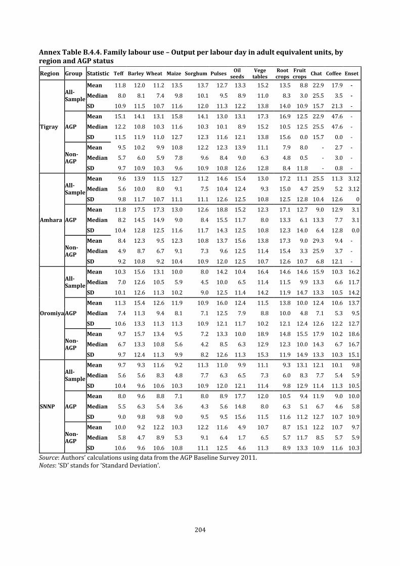
204
Annex Table B.4.4. Family labour use – Output per labour day in adult equivalent units, by region and AGP status
Region Group Statistic Teff Barley Wheat Maize Sorghum Pulses Oil
seeds Vege
tables Root crops
Fruit crops
Chat Coffee Enset
Tigray
All-Sample
Mean 11.8 12.0 11.2 13.5 13.7 12.7 13.3 15.2 13.5 8.8 22.9 17.9 -
Median 8.0 8.1 7.4 9.8 10.1 9.5 8.9 11.0 8.3 3.0 25.5 3.5 -
SD 10.9 11.5 10.7 11.6 12.0 11.3 12.2 13.8 14.0 10.9 15.7 21.3 -
AGP
Mean 15.1 14.1 13.1 15.8 14.1 13.0 13.1 17.3 16.9 12.5 22.9 47.6 -
Median 12.2 10.8 10.3 11.6 10.3 10.1 8.9 15.2 10.5 12.5 25.5 47.6 -
SD 11.5 11.9 11.0 12.7 12.3 11.6 12.1 13.8 15.6 0.0 15.7 0.0 -
Non-AGP
Mean 9.5 10.2 9.9 10.8 12.2 12.3 13.9 11.1 7.9 8.0 - 2.7 -
Median 5.7 6.0 5.9 7.8 9.6 8.4 9.0 6.3 4.8 0.5 - 3.0 -
SD 9.7 10.9 10.3 9.6 10.9 10.8 12.6 12.8 8.4 11.8 - 0.8 -
Amhara
All-Sample
Mean 9.6 13.9 11.5 12.7 11.2 14.6 15.4 13.0 17.2 11.1 25.5 11.3 3.12
Median 5.6 10.0 8.0 9.1 7.5 10.4 12.4 9.3 15.0 4.7 25.9 5.2 3.12
SD 9.8 11.7 10.7 11.1 11.1 12.6 12.5 10.8 12.5 12.8 10.4 12.6 0
AGP
Mean 11.8 17.5 17.3 13.0 12.6 18.8 15.2 12.3 17.1 12.7 9.0 12.9 3.1
Median 8.2 14.5 14.9 9.0 8.4 15.5 11.7 8.0 13.3 6.1 13.3 7.7 3.1
SD 10.4 12.8 12.5 11.6 11.7 14.3 12.5 10.8 12.3 14.0 6.4 12.8 0.0
Non-AGP
Mean 8.4 12.3 9.5 12.3 10.8 13.7 15.6 13.8 17.3 9.0 29.3 9.4 -
Median 4.9 8.7 6.7 9.1 7.3 9.6 12.5 11.4 15.4 3.3 25.9 3.7 -
SD 9.2 10.8 9.2 10.4 10.9 12.0 12.5 10.7 12.6 10.7 6.8 12.1 -
Oromiya
All-Sample
Mean 10.3 15.6 13.1 10.0 8.0 14.2 10.4 16.4 14.6 14.6 15.9 10.3 16.2
Median 7.0 12.6 10.5 5.9 4.5 10.0 6.5 11.4 11.5 9.9 13.3 6.6 11.7
SD 10.1 12.6 11.3 10.2 9.0 12.5 11.4 14.2 11.9 14.7 13.3 10.5 14.2
AGP
Mean 11.3 15.4 12.6 11.9 10.9 16.0 12.4 11.5 13.8 10.0 12.4 10.6 13.7
Median 7.4 11.3 9.4 8.1 7.1 12.5 7.9 8.8 10.0 4.8 7.1 5.3 9.5
SD 10.6 13.3 11.3 11.3 10.9 12.1 11.7 10.2 12.1 12.4 12.6 12.2 12.7
Non-AGP
Mean 9.7 15.7 13.4 9.5 7.2 13.3 10.0 18.9 14.8 15.5 17.9 10.2 18.6
Median 6.7 13.3 10.8 5.6 4.2 8.5 6.3 12.9 12.3 10.0 14.3 6.7 16.7
SD 9.7 12.4 11.3 9.9 8.2 12.6 11.3 15.3 11.9 14.9 13.3 10.3 15.1
SNNP
All-Sample
Mean 9.7 9.3 11.6 9.2 11.3 11.0 9.9 11.1 9.3 13.1 12.1 10.1 9.8
Median 5.6 5.6 8.3 4.8 7.7 6.3 6.5 7.3 6.0 8.3 7.7 5.4 5.9
SD 10.4 9.6 10.6 10.3 10.9 12.0 12.1 11.4 9.8 12.9 11.4 11.3 10.5
AGP
Mean 8.0 9.6 8.8 7.1 8.0 8.9 17.7 12.0 10.5 9.4 11.9 9.0 10.0
Median 5.5 6.3 5.4 3.6 4.3 5.6 14.8 8.0 6.3 5.1 6.7 4.6 5.8
SD 9.0 9.8 9.8 9.0 9.5 9.5 15.6 11.5 11.6 11.2 12.7 10.7 10.9
Non-AGP
Mean 10.0 9.2 12.2 10.3 12.2 11.6 4.9 10.7 8.7 15.1 12.2 10.7 9.7
Median 5.8 4.7 8.9 5.3 9.1 6.4 1.7 6.5 5.7 11.7 8.5 5.7 5.9
SD 10.6 9.6 10.6 10.8 11.1 12.5 4.6 11.3 8.9 13.3 10.9 11.6 10.3
Source: Authors’ calculations using data from the AGP Baseline Survey 2011. Notes: ‘SD’ stands for ‘Standard Deviation’.
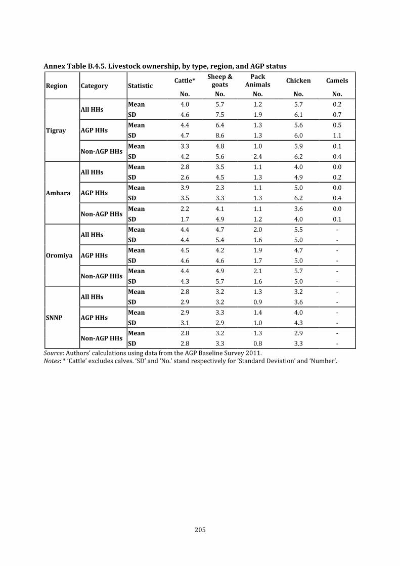
205
Annex Table B.4.5. Livestock ownership, by type, region, and AGP status
Region Category Statistic Cattle*
Sheep & goats
Pack Animals
Chicken Camels
No. No. No. No. No.
Tigray
All HHs Mean 4.0 5.7 1.2 5.7 0.2
SD 4.6 7.5 1.9 6.1 0.7
AGP HHs Mean 4.4 6.4 1.3 5.6 0.5
SD 4.7 8.6 1.3 6.0 1.1
Non-AGP HHs Mean 3.3 4.8 1.0 5.9 0.1
SD 4.2 5.6 2.4 6.2 0.4
Amhara
All HHs Mean 2.8 3.5 1.1 4.0 0.0
SD 2.6 4.5 1.3 4.9 0.2
AGP HHs Mean 3.9 2.3 1.1 5.0 0.0
SD 3.5 3.3 1.3 6.2 0.4
Non-AGP HHs Mean 2.2 4.1 1.1 3.6 0.0
SD 1.7 4.9 1.2 4.0 0.1
Oromiya
All HHs Mean 4.4 4.7 2.0 5.5 -
SD 4.4 5.4 1.6 5.0 -
AGP HHs Mean 4.5 4.2 1.9 4.7 -
SD 4.6 4.6 1.7 5.0 -
Non-AGP HHs Mean 4.4 4.9 2.1 5.7 -
SD 4.3 5.7 1.6 5.0 -
SNNP
All HHs Mean 2.8 3.2 1.3 3.2 -
SD 2.9 3.2 0.9 3.6 -
AGP HHs Mean 2.9 3.3 1.4 4.0 -
SD 3.1 2.9 1.0 4.3 -
Non-AGP HHs Mean 2.8 3.2 1.3 2.9 -
SD 2.8 3.3 0.8 3.3 -
Source: Authors’ calculations using data from the AGP Baseline Survey 2011. Notes: * ‘Cattle’ excludes calves. ‘SD’ and ‘No.’ stand respectively for ‘Standard Deviation’ and ‘Number’.
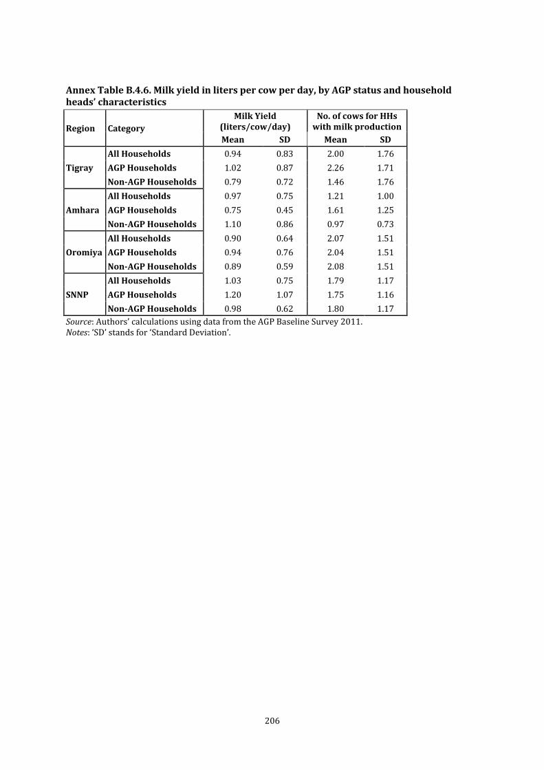
206
Annex Table B.4.6. Milk yield in liters per cow per day, by AGP status and household heads’ characteristics
Region Category
Milk Yield (liters/cow/day)
No. of cows for HHs with milk production
Mean SD Mean SD
Tigray
All Households 0.94 0.83 2.00 1.76
AGP Households 1.02 0.87 2.26 1.71
Non-AGP Households 0.79 0.72 1.46 1.76
Amhara
All Households 0.97 0.75 1.21 1.00
AGP Households 0.75 0.45 1.61 1.25
Non-AGP Households 1.10 0.86 0.97 0.73
Oromiya
All Households 0.90 0.64 2.07 1.51
AGP Households 0.94 0.76 2.04 1.51
Non-AGP Households 0.89 0.59 2.08 1.51
SNNP
All Households 1.03 0.75 1.79 1.17
AGP Households 1.20 1.07 1.75 1.16
Non-AGP Households 0.98 0.62 1.80 1.17
Source: Authors’ calculations using data from the AGP Baseline Survey 2011. Notes: ‘SD’ stands for ‘Standard Deviation’.
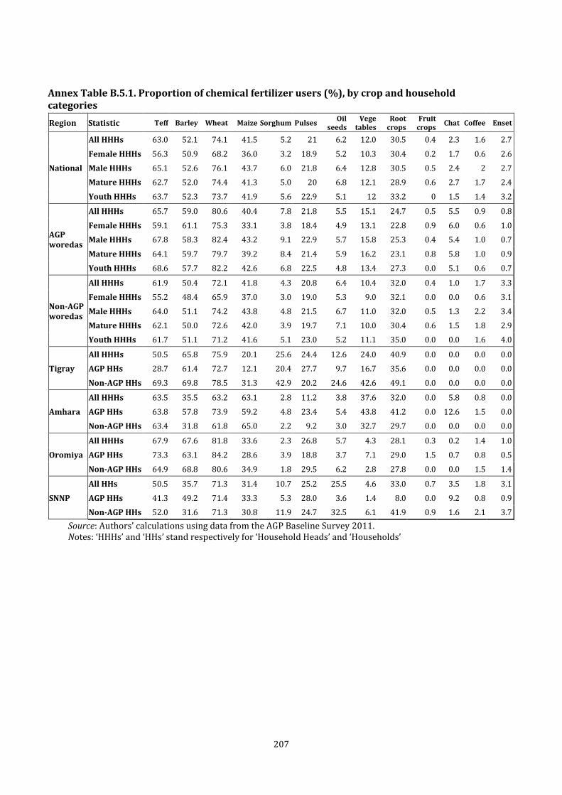
207
Annex Table B.5.1. Proportion of chemical fertilizer users (%), by crop and household categories
Region Statistic Teff Barley Wheat Maize Sorghum Pulses Oil
seeds Vege
tables Root
crops Fruit
crops Chat Coffee Enset
National
All HHHs 63.0 52.1 74.1 41.5 5.2 21 6.2 12.0 30.5 0.4 2.3 1.6 2.7
Female HHHs 56.3 50.9 68.2 36.0 3.2 18.9 5.2 10.3 30.4 0.2 1.7 0.6 2.6
Male HHHs 65.1 52.6 76.1 43.7 6.0 21.8 6.4 12.8 30.5 0.5 2.4 2 2.7
Mature HHHs 62.7 52.0 74.4 41.3 5.0 20 6.8 12.1 28.9 0.6 2.7 1.7 2.4
Youth HHHs 63.7 52.3 73.7 41.9 5.6 22.9 5.1 12 33.2 0 1.5 1.4 3.2
AGP woredas
All HHHs 65.7 59.0 80.6 40.4 7.8 21.8 5.5 15.1 24.7 0.5 5.5 0.9 0.8
Female HHHs 59.1 61.1 75.3 33.1 3.8 18.4 4.9 13.1 22.8 0.9 6.0 0.6 1.0
Male HHHs 67.8 58.3 82.4 43.2 9.1 22.9 5.7 15.8 25.3 0.4 5.4 1.0 0.7
Mature HHHs 64.1 59.7 79.7 39.2 8.4 21.4 5.9 16.2 23.1 0.8 5.8 1.0 0.9
Youth HHHs 68.6 57.7 82.2 42.6 6.8 22.5 4.8 13.4 27.3 0.0 5.1 0.6 0.7
Non-AGP woredas
All HHHs 61.9 50.4 72.1 41.8 4.3 20.8 6.4 10.4 32.0 0.4 1.0 1.7 3.3
Female HHHs 55.2 48.4 65.9 37.0 3.0 19.0 5.3 9.0 32.1 0.0 0.0 0.6 3.1
Male HHHs 64.0 51.1 74.2 43.8 4.8 21.5 6.7 11.0 32.0 0.5 1.3 2.2 3.4
Mature HHHs 62.1 50.0 72.6 42.0 3.9 19.7 7.1 10.0 30.4 0.6 1.5 1.8 2.9
Youth HHHs 61.7 51.1 71.2 41.6 5.1 23.0 5.2 11.1 35.0 0.0 0.0 1.6 4.0
Tigray
All HHHs 50.5 65.8 75.9 20.1 25.6 24.4 12.6 24.0 40.9 0.0 0.0 0.0 0.0
AGP HHs 28.7 61.4 72.7 12.1 20.4 27.7 9.7 16.7 35.6 0.0 0.0 0.0 0.0
Non-AGP HHs 69.3 69.8 78.5 31.3 42.9 20.2 24.6 42.6 49.1 0.0 0.0 0.0 0.0
Amhara
All HHHs 63.5 35.5 63.2 63.1 2.8 11.2 3.8 37.6 32.0 0.0 5.8 0.8 0.0
AGP HHs 63.8 57.8 73.9 59.2 4.8 23.4 5.4 43.8 41.2 0.0 12.6 1.5 0.0
Non-AGP HHs 63.4 31.8 61.8 65.0 2.2 9.2 3.0 32.7 29.7 0.0 0.0 0.0 0.0
Oromiya
All HHHs 67.9 67.6 81.8 33.6 2.3 26.8 5.7 4.3 28.1 0.3 0.2 1.4 1.0
AGP HHs 73.3 63.1 84.2 28.6 3.9 18.8 3.7 7.1 29.0 1.5 0.7 0.8 0.5
Non-AGP HHs 64.9 68.8 80.6 34.9 1.8 29.5 6.2 2.8 27.8 0.0 0.0 1.5 1.4
SNNP
All HHs 50.5 35.7 71.3 31.4 10.7 25.2 25.5 4.6 33.0 0.7 3.5 1.8 3.1
AGP HHs 41.3 49.2 71.4 33.3 5.3 28.0 3.6 1.4 8.0 0.0 9.2 0.8 0.9
Non-AGP HHs 52.0 31.6 71.3 30.8 11.9 24.7 32.5 6.1 41.9 0.9 1.6 2.1 3.7
Source: Authors’ calculations using data from the AGP Baseline Survey 2011. Notes: ‘HHHs’ and ‘HHs’ stand respectively for ‘Household Heads’ and ‘Households’

208
Annex Table B.5.2. Proportion of chemical fertilizer users and average application rate of fertilizer for all farmers and users only (in kg), by household categories and AGP status
Region Household type Chemical
fertilizer users (%)
DAP - All farmers
DAP - User
farmers only
Urea - All farmers
Urea - User
farmers only
DAP+Urea - All
farmers
DAP+Urea - User
farmers only
Tigray
All Households 56.8 12.1 22.5 8.4 19.5 20.4 36.4
AGP Households 78.0 8.5 21.0 6.7 19.4 15.3 34.9
Non-AGP Households
44.0 17.8 23.7 11.0 19.5 28.9 37.8
Amhara
All Households 58.9 14.1 30.2 13.0 26.5 27.1 50.6
AGP Households 56.8 19.5 41.1 18.6 33.0 38.1 62.1
Non-AGP Households
65.8 11.2 24.2 10.0 22.1 21.1 42.8
Oromiya
All Households 66.4 24.8 40.6 11.6 35.0 36.4 56.7
AGP Households 64.1 24.2 39.8 15.1 34.7 39.3 57.1
Non-AGP Households
73.6 25.0 40.8 10.4 35.1 35.4 56.5
SNNP
All Households 40.7 7.8 20.5 3.5 17.7 11.2 28.5
AGP Households 64.1 6.3 23.2 2.4 18.6 8.7 30.8
Non-AGP Households
73.6 8.3 19.8 3.8 17.6 12.1 28.0
Source: Authors’ calculations using data from the AGP Baseline Survey 2011.
Annex Table B.5.3. Improved seed, irrigation, and soil conservation use by region and AGP status (% of households)
Region Household type
Improved seed users
Improved seed use –
All Farmers
Improved seed use –
User Farmers Only
Irrigation Soil
conservation
(%) (kg/ha) (kg/ha) (%) (%)
Tigray
All HHs 18.4 1.73 17.7 8.60 84.6
AGP HHs 12.0 1.15 18.2 7.50 80.1
Non-AGP HHs 29.0 2.69 17.0 10.40 92.3
Amhara
All HHs 33.8 3.67 11.8 7.30 88.2
AGP HHs 45.9 1.44 12.4 12.30 81.3
Non-AGP HHs 30.1 3.44 10.6 5.80 90.3
Oromiya
All HHs 21.5 1.68 9.9 3.40 76.1
AGP HHs 13.2 1.04 9.9 8.10 80.1
Non-AGP HHs 24.2 1.89 10.3 1.90 74.8
SNNP
All HHs 13.1 1.21 11.4 1.80 47.5
AGP HHs 15.3 1.10 11.9 1.23 32.2
Non-AGP HHs 12.6 1.24 9.3 1.95 51.0
Source: Authors’ calculations using data from the AGP Baseline Survey 2011. Notes: ‘HHs’ stands for ‘Households’.
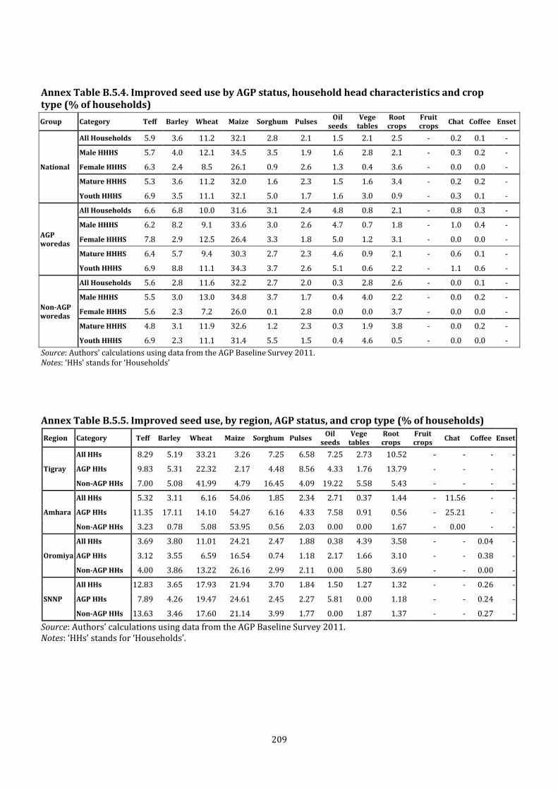
209
Annex Table B.5.4. Improved seed use by AGP status, household head characteristics and crop type (% of households)
Group Category Teff Barley Wheat Maize Sorghum Pulses Oil
seeds Vege
tables Root crops
Fruit crops
Chat Coffee Enset
National
All Households 5.9 3.6 11.2 32.1 2.8 2.1 1.5 2.1 2.5 - 0.2 0.1 -
Male HHHS 5.7 4.0 12.1 34.5 3.5 1.9 1.6 2.8 2.1 - 0.3 0.2 -
Female HHHS 6.3 2.4 8.5 26.1 0.9 2.6 1.3 0.4 3.6 - 0.0 0.0 -
Mature HHHS 5.3 3.6 11.2 32.0 1.6 2.3 1.5 1.6 3.4 - 0.2 0.2 -
Youth HHHS 6.9 3.5 11.1 32.1 5.0 1.7 1.6 3.0 0.9 - 0.3 0.1 -
AGP woredas
All Households 6.6 6.8 10.0 31.6 3.1 2.4 4.8 0.8 2.1 - 0.8 0.3 -
Male HHHS 6.2 8.2 9.1 33.6 3.0 2.6 4.7 0.7 1.8 - 1.0 0.4 -
Female HHHS 7.8 2.9 12.5 26.4 3.3 1.8 5.0 1.2 3.1 - 0.0 0.0 -
Mature HHHS 6.4 5.7 9.4 30.3 2.7 2.3 4.6 0.9 2.1 - 0.6 0.1 -
Youth HHHS 6.9 8.8 11.1 34.3 3.7 2.6 5.1 0.6 2.2 - 1.1 0.6 -
Non-AGP woredas
All Households 5.6 2.8 11.6 32.2 2.7 2.0 0.3 2.8 2.6 - 0.0 0.1 -
Male HHHS 5.5 3.0 13.0 34.8 3.7 1.7 0.4 4.0 2.2 - 0.0 0.2 -
Female HHHS 5.6 2.3 7.2 26.0 0.1 2.8 0.0 0.0 3.7 - 0.0 0.0 -
Mature HHHS 4.8 3.1 11.9 32.6 1.2 2.3 0.3 1.9 3.8 - 0.0 0.2 -
Youth HHHS 6.9 2.3 11.1 31.4 5.5 1.5 0.4 4.6 0.5 - 0.0 0.0 -
Source: Authors’ calculations using data from the AGP Baseline Survey 2011. Notes: ‘HHs’ stands for ‘Households’
Annex Table B.5.5. Improved seed use, by region, AGP status, and crop type (% of households)
Region Category Teff Barley Wheat Maize Sorghum Pulses Oil
seeds Vege
tables Root crops
Fruit crops
Chat Coffee Enset
Tigray
All HHs 8.29 5.19 33.21 3.26 7.25 6.58 7.25 2.73 10.52 - - - -
AGP HHs 9.83 5.31 22.32 2.17 4.48 8.56 4.33 1.76 13.79 - - - -
Non-AGP HHs 7.00 5.08 41.99 4.79 16.45 4.09 19.22 5.58 5.43 - - - -
Amhara
All HHs 5.32 3.11 6.16 54.06 1.85 2.34 2.71 0.37 1.44 - 11.56 - -
AGP HHs 11.35 17.11 14.10 54.27 6.16 4.33 7.58 0.91 0.56 - 25.21 - -
Non-AGP HHs 3.23 0.78 5.08 53.95 0.56 2.03 0.00 0.00 1.67 - 0.00 - -
Oromiya
All HHs 3.69 3.80 11.01 24.21 2.47 1.88 0.38 4.39 3.58 - - 0.04 -
AGP HHs 3.12 3.55 6.59 16.54 0.74 1.18 2.17 1.66 3.10 - - 0.38 -
Non-AGP HHs 4.00 3.86 13.22 26.16 2.99 2.11 0.00 5.80 3.69 - - 0.00 -
SNNP
All HHs 12.83 3.65 17.93 21.94 3.70 1.84 1.50 1.27 1.32 - - 0.26 -
AGP HHs 7.89 4.26 19.47 24.61 2.45 2.27 5.81 0.00 1.18 - - 0.24 -
Non-AGP HHs 13.63 3.46 17.60 21.14 3.99 1.77 0.00 1.87 1.37 - - 0.27 -
Source: Authors’ calculations using data from the AGP Baseline Survey 2011. Notes: ‘HHs’ stands for ‘Households’.

210
Annex Table B.5.6. Mean difference test – Proportion of households using improved seed, by crop type and household categories
Region Category Statis tic
Teff Barley Wheat Maize Sorghum Pulses Oil
seeds Vege
tables Root
Crops Fruit Crops
Chat Coffee Enset
National
Male HHHs vs. Female HHHs
MD -0.5 1.6 3.5 8.4 2.6 -0.7 0.3 2.4 -1.5 - 0.3 0.2 -
Sig. *** ** *
Mature HHHs vs. Youth HHHs
MD -1.6 0.1 0.1 -0.1 -3.4 0.6 -0.1 -1.4 2.5 - -0.1 0.1 -
Sig.
*
AGP HHs vs. Non-AGP HHs
MD 1.0 4.0 -1.6 -0.6 0.4 0.4 4.4 -2.0 -0.5 - 0.8 0.1 -
Sig. *
AGP woredas
Male HHHs vs. Female HHHs
MD -1.6 5.2 -3.3 7.2 -0.3 0.7 -0.4 -0.5 -1.2 - 1.0 0.4 -
Sig. ** ***
*
Mature HHHs vs. Youth HHHs
MD -0.5 -3.1 -1.8 -4.0 -1.0 -0.3 -0.5 0.3 -0.1 - -0.5 -0.5 -
Sig. * **
Source: Authors’ calculations using data from the AGP Baseline Survey 2011. Note: ‘HHHs’ and ‘HHs’ stand respectively for ‘Headed Households’ and ‘Households’. ‘MD’ and ‘Sig.’ stand for ‘Mean Difference’ and ‘Significance’, respectively. ‘Mean difference’ refers to the difference between the mean values of the variable in question wit in the groups being compared. ‘Significance’ reports the result of a corresponding (two-tailed) test of whether such difference is statistically different from zero. ***, ** and * indicate that the corresponding mean difference is statistically significant at 1 percent, 5 percent and 10 percent, respectively.
Annex Table B.5.7. Percentage of households that purchased improved seed with credit and reasons for not using credit, by AGP status and household categories
Region Category Purchased input with
credit
Reason for not purchasing with credit
No need for
credit
Asked for credit but
was refused
Credit provider
not available
Fear of being
rejected
Lack of assets for collateral
Fear of losing
asset held as
collateral
Fear of not being able
to pay back
Interest rate too
high
National
All HHs 7.3 29.8 11.1 51.5 1.0 0.6 0.3 2.9 2.7
Male HHHs 7.3 31.1 10.2 52.0 0.8 0.4 0.4 2.5 2.7
Female HHHs 7.1 25.4 14.2 50.0 2.0 1.4 0.0 4.3 2.7
Mature HHHs 7.8 27.4 12.4 52.5 0.9 0.8 0.5 2.4 3.2
Youth HHHs 6.4 34.1 8.8 49.9 1.3 0.4 0.0 3.8 1.9
AGP woredas
All HHs 8.6 35.3 11.9 45.8 0.9 0.4 0.1 1.7 3.2
Male HHHs 9.1 36.0 12.1 45.0 1.0 0.4 0.1 1.3 3.2
Female HHHs 6.7 32.9 10.9 48.5 0.8 0.5 0.0 3.1 3.2
Mature HHHs 9.5 32.9 12.4 46.4 1.4 0.7 0.1 1.8 3.8
Youth HHHs 7.0 39.6 10.8 44.8 0.2 0.0 0.0 1.6 2.2
Non-AGP woredas
All HHs 6.9 28.3 10.9 52.7 1.1 0.7 0.4 3.2 2.6
Male HHHs 6.8 29.8 9.7 53.7 0.7 0.4 0.5 2.8 2.6
Female HHHs 7.1 23.2 15.0 49.3 2.3 1.6 0.0 4.6 2.5
Mature HHHs 7.2 26.0 12.4 53.6 0.8 0.8 0.6 2.5 3.0
Youth HHHs 6.2 32.5 8.2 51.1 1.6 0.4 0.0 4.4 1.8
Source: Authors’ calculations using data from the AGP Baseline Survey 2011. Notes: ‘HHHs’ and ‘HHs’ stand respectively for ‘Headed Households’ and ‘Households’

211
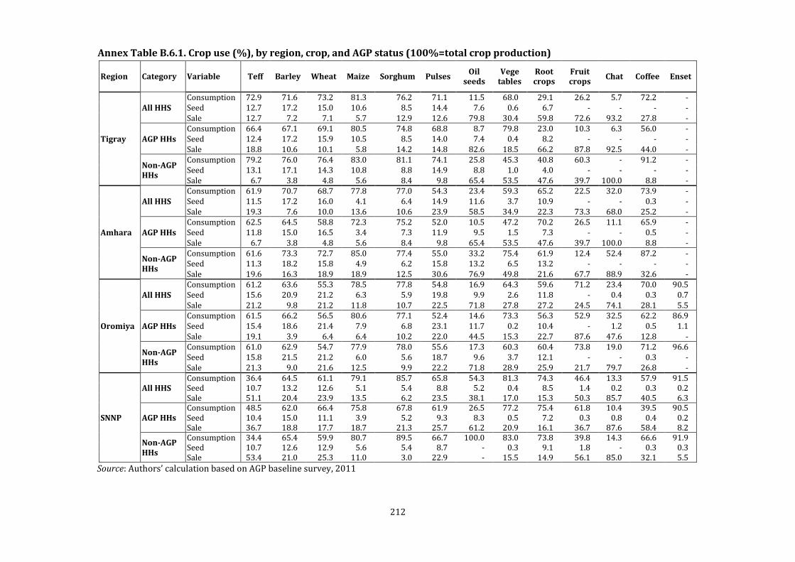
212
Annex Table B.6.1. Crop use (%), by region, crop, and AGP status (100%=total crop production)
Region Category Variable Teff Barley Wheat Maize Sorghum Pulses Oil
seeds Vege
tables Root crops
Fruit crops
Chat Coffee Enset
Tigray
All HHS Consumption 72.9 71.6 73.2 81.3 76.2 71.1 11.5 68.0 29.1 26.2 5.7 72.2 - Seed 12.7 17.2 15.0 10.6 8.5 14.4 7.6 0.6 6.7 - - - - Sale 12.7 7.2 7.1 5.7 12.9 12.6 79.8 30.4 59.8 72.6 93.2 27.8 -
AGP HHs Consumption 66.4 67.1 69.1 80.5 74.8 68.8 8.7 79.8 23.0 10.3 6.3 56.0 - Seed 12.4 17.2 15.9 10.5 8.5 14.0 7.4 0.4 8.2 - - - - Sale 18.8 10.6 10.1 5.8 14.2 14.8 82.6 18.5 66.2 87.8 92.5 44.0 -
Non-AGP HHs
Consumption 79.2 76.0 76.4 83.0 81.1 74.1 25.8 45.3 40.8 60.3 - 91.2 - Seed 13.1 17.1 14.3 10.8 8.8 14.9 8.8 1.0 4.0 - - - - Sale 6.7 3.8 4.8 5.6 8.4 9.8 65.4 53.5 47.6 39.7 100.0 8.8 -
Amhara
All HHS Consumption 61.9 70.7 68.7 77.8 77.0 54.3 23.4 59.3 65.2 22.5 32.0 73.9 - Seed 11.5 17.2 16.0 4.1 6.4 14.9 11.6 3.7 10.9 - - 0.3 - Sale 19.3 7.6 10.0 13.6 10.6 23.9 58.5 34.9 22.3 73.3 68.0 25.2 -
AGP HHs Consumption 62.5 64.5 58.8 72.3 75.2 52.0 10.5 47.2 70.2 26.5 11.1 65.9 - Seed 11.8 15.0 16.5 3.4 7.3 11.9 9.5 1.5 7.3 - - 0.5 - Sale 6.7 3.8 4.8 5.6 8.4 9.8 65.4 53.5 47.6 39.7 100.0 8.8 -
Non-AGP HHs
Consumption 61.6 73.3 72.7 85.0 77.4 55.0 33.2 75.4 61.9 12.4 52.4 87.2 - Seed 11.3 18.2 15.8 4.9 6.2 15.8 13.2 6.5 13.2 - - - - Sale 19.6 16.3 18.9 18.9 12.5 30.6 76.9 49.8 21.6 67.7 88.9 32.6 -
Oromiya
All HHS Consumption 61.2 63.6 55.3 78.5 77.8 54.8 16.9 64.3 59.6 71.2 23.4 70.0 90.5 Seed 15.6 20.9 21.2 6.3 5.9 19.8 9.9 2.6 11.8 - 0.4 0.3 0.7 Sale 21.2 9.8 21.2 11.8 10.7 22.5 71.8 27.8 27.2 24.5 74.1 28.1 5.5
AGP HHs Consumption 61.5 66.2 56.5 80.6 77.1 52.4 14.6 73.3 56.3 52.9 32.5 62.2 86.9 Seed 15.4 18.6 21.4 7.9 6.8 23.1 11.7 0.2 10.4 - 1.2 0.5 1.1 Sale 19.1 3.9 6.4 6.4 10.2 22.0 44.5 15.3 22.7 87.6 47.6 12.8 -
Non-AGP HHs
Consumption 61.0 62.9 54.7 77.9 78.0 55.6 17.3 60.3 60.4 73.8 19.0 71.2 96.6 Seed 15.8 21.5 21.2 6.0 5.6 18.7 9.6 3.7 12.1 - - 0.3 - Sale 21.3 9.0 21.6 12.5 9.9 22.2 71.8 28.9 25.9 21.7 79.7 26.8 -
SNNP
All HHS Consumption 36.4 64.5 61.1 79.1 85.7 65.8 54.3 81.3 74.3 46.4 13.3 57.9 91.5 Seed 10.7 13.2 12.6 5.1 5.4 8.8 5.2 0.4 8.5 1.4 0.2 0.3 0.2 Sale 51.1 20.4 23.9 13.5 6.2 23.5 38.1 17.0 15.3 50.3 85.7 40.5 6.3
AGP HHs Consumption 48.5 62.0 66.4 75.8 67.8 61.9 26.5 77.2 75.4 61.8 10.4 39.5 90.5 Seed 10.4 15.0 11.1 3.9 5.2 9.3 8.3 0.5 7.2 0.3 0.8 0.4 0.2 Sale 36.7 18.8 17.7 18.7 21.3 25.7 61.2 20.9 16.1 36.7 87.6 58.4 8.2
Non-AGP HHs
Consumption 34.4 65.4 59.9 80.7 89.5 66.7 100.0 83.0 73.8 39.8 14.3 66.6 91.9 Seed 10.7 12.6 12.9 5.6 5.4 8.7 - 0.3 9.1 1.8 - 0.3 0.3 Sale 53.4 21.0 25.3 11.0 3.0 22.9 - 15.5 14.9 56.1 85.0 32.1 5.5
Source: Authors’ calculation based on AGP baseline survey, 2011

213
Annex Table B.6.2. Average revenue (ETB) from crop sale, by region, AGP status, and crop type
Region Categories Teff Barley Wheat Maize Sorghum Pulses Oil
seeds Vege
tables Root crops
Fruit crops
Chat Coffee Enset
Tigray
All HHs 512 167 195 91 550 259 6819 475 3836 68 436 236 0
AGP HHs 527 202 266 109 642 351 7508 272 5277 111 484 409 0
Non-AGP HHs 497 133 142 57 245 138 3189 870 1059 0 7 33 0
Amhara
All HHs 564 221 361 603 344 699 5478 1359 421 254 320 2196 0
AGP HHs 632 536 885 977 527 1037 12192 2225 463 337 463 2898 0
Non-AGP HHs 524 85 147 103 304 601 358 215 393 40 181 1025 0
Oromiya
All HHs 792 500 1603 602 326 722 1228 258 1082 282 1183 7549 58
AGP HHs 1120 736 1440 372 584 1121 1958 171 1337 585 2423 6532 93
Non-AGP HHs 597 433 1683 659 254 584 1090 297 1019 238 589 7707 0
SNNP
All HHs 742 337 604 256 100 623 188 43 136 124 2547 5420 67
AGP HHs 532 413 480 388 422 562 302 54 100 85 8521 7765 82
Non-AGP HHs 776 309 632 193 32 637 0 39 154 141 440 4318 61
Source: Authors’ calculation based on AGP baseline survey, 2011. Note: ‘HHs’ stands for ‘Households’.

214
Annex Table B.6.3. Percentage of households who sold their output, by crop type, household categories, and AGP status
Group Categories Teff Barley Wheat Maize Sorghum Pulses
Oil seeds
Vege tables
Root crops
Fruit crops
Chat Coffee Enset
National
All HHs 20.0 9.3 14.6 16.4 6.4 19.0 8.4 3.4 8.1 3.7 5.2 10.4 3.7
Female HHHs 15.8 9.1 12.2 13.7 5.6 15.7 6.9 3.5 7.0 3.0 4.2 9.2 4.0
Male HHHs 21.7 9.3 15.6 17.6 6.7 20.3 9.0 3.4 8.6 4.0 5.7 11.0 3.5
Mature HHHs 20.8 9.0 13.8 16.1 6.4 19.3 8.1 3.5 8.4 3.8 5.4 10.7 3.8
Youth HHHs 18.6 9.8 15.9 17.0 6.4 18.4 8.8 3.3 7.7 3.5 5.0 9.9 3.3
AGP woredas
All HHs 24.6 9.1 16.4 18.0 8.7 17.1 9.6 6.0 7.4 4.0 6.5 9.5 5.3
Female HHHs 17.6 8.5 14.6 17.7 5.3 14.1 5.5 4.8 6.1 3.3 4.8 12.6 5.4
Male HHHs 25.3 11.9 18.7 24.4 7.9 19.7 9.9 5.5 9.3 3.6 5.6 12.0 4.9
Mature HHHs 23.1 9.9 16.9 22.6 7.5 17.9 8.5 5.0 8.2 3.6 5.3 13.1 5.0
Youth HHHs 23.0 12.6 18.5 22.3 6.5 18.3 8.8 5.7 8.7 3.4 5.3 10.6 5.2
Non-AGP woredas
All HHs 18.6 9.3 14.0 16.0 5.7 19.5 8.0 2.6 8.3 3.6 4.8 10.7 3.2
Female HHHs 15.1 9.3 11.2 12.2 5.8 16.4 7.4 3.0 7.3 2.9 4.0 7.8 3.4
Male HHHs 20.3 8.3 14.3 14.8 6.3 20.6 8.6 2.5 8.3 4.1 5.7 10.6 3.0
Mature HHHs 19.9 8.6 12.5 13.5 6.0 19.9 7.9 2.8 8.4 3.9 5.4 9.8 3.4
Youth HHHs 16.8 8.6 14.9 14.9 6.3 18.4 8.8 2.3 7.2 3.5 4.9 9.7 2.6 Source: Authors’ calculation based on AGP baseline survey, 2011. Note: ‘HHs’ and ‘HHHs’ stand respectively for ‘Households’ and ‘Headed Households’.

215
Annex Table B.6.4. Percentage of households who sold their output, by crop type, region, and AGP status
Region Categories Teff Barley Wheat Maize Sorghum Pulses Oil
seeds Vege
tables Root crops
Fruit crops
Chat Coffee Enset
Tigray
All HHs 10.9 7.9 8.7 3.7 17.5 5.2 17.4 1.1 3.6 0.1 1.3 0.4 -
AGP HHs 11.3 8.1 8.0 3.6 23.7 5.8 24.3 0.7 4.2 0.2 2.0 0.6 -
Non-AGP HHs 10.2 7.6 9.8 3.9 7.7 4.1 6.3 1.7 2.7 0.0 0.2 0.2 -
Amhara
All HHs 27.2 9.2 12.2 20.7 9.0 27.3 8.2 3.0 7.9 1.0 0.3 1.3 -
AGP HHs 29.3 14.3 18.3 43.8 5.3 19.4 12.5 6.4 8.4 1.9 0.4 3.0 -
Non-AGP HHs 26.1 6.5 8.8 8.3 10.9 31.6 5.8 1.2 7.6 0.5 0.2 0.4 -
Oromiya
All HHs 18.4 10.2 19.3 18.2 7.1 17.4 12.7 2.2 9.0 2.9 4.4 8.0 0.9
AGP HHs 28.9 10.1 25.6 11.6 8.7 23.2 7.9 2.9 8.4 2.2 5.3 5.9 3.7
Non-AGP HHs 15.0 10.2 17.2 20.3 6.6 15.5 14.2 2.0 9.2 3.1 4.1 8.7 0.0
SNNP
All HHs 16.3 7.8 9.4 10.3 1.4 14.6 0.1 6.2 7.2 8.2 12.3 25.2 12.6
AGP HHs 7.7 8.0 5.2 15.2 3.1 10.8 0.5 8.8 9.5 8.8 13.0 38.4 15.6
Non-AGP HHs 19.3 7.8 10.9 8.6 0.8 15.9 0.0 5.3 6.4 8.0 12.0 20.6 11.6
Source: Authors’ calculation based on AGP baseline survey, 2011. Note: ‘HHs’ stands for ‘Households’.
Annex Table B.6.5. Percentage of transportation cost from total revenue, by region, AGP status and crop type
Region Category Teff Barley Wheat Maize Sorghum Pulses Oil
seeds Vege
tables Root crops
Fruit crops
Chat Coffee Enset
Tigray
All HHs 0.5 1.8 0.6 1.2 1.2 0.4 1.2 6.6 5.2 0.6 0.8 -
AGP HHs 0.7 2.3 0.4 1.3 1.2 0.4 1.3 1.2 1.0 - 0.8 -
Non-AGP HHs 0.2 0.2 0.9 0.9 0.3 0.1 0.2 15.6 14.7 4.8 - -
Amhara
All HHs 0.3 0.2 0.3 0.8 1.1 0.1 1.5 0.4 0.8 0.5 0.8 0.0
AGP HHs 0.5 0.3 0.3 0.8 3.5 0.2 1.5 0.4 1.1 0.6 1.1 -
Non-AGP HHs 0.2 - 0.3 0.2 0.2 0.1 0.2 0.5 0.4 - - 0.1
Oromiya
All HHs 1.3 0.6 1.2 2.1 0.8 0.6 0.4 13.5 3.7 0.0 0.2 3.2 1.9
AGP HHs 0.3 1.0 0.4 1.6 0.4 0.4 0.3 0.8 13.0 0.2 0.1 0.3 1.9
Non-AGP HHs 2.0 0.4 1.7 2.1 1.0 0.7 0.4 15.0 1.1 - 0.6 3.9
SNNP
All HHs 2.0 11.2 0.7 2.4 1.7 2.1 0.8 4.8 1.5 0.7 4.8 1.5 2.3
AGP HHs 0.9 2.2 1.0 1.8 2.0 1.6 1.2 3.1 2.6 0.6 3.5 0.6 1.5
Non-AGP HHs 2.2 15.8 0.7 2.9 0.9 2.2 0.5 5.1 1.2 0.7 5.9 2.1 2.5
Source: Authors’ calculation based on AGP baseline survey, 2011. Note: ‘HHs’ stands for ‘Households’.
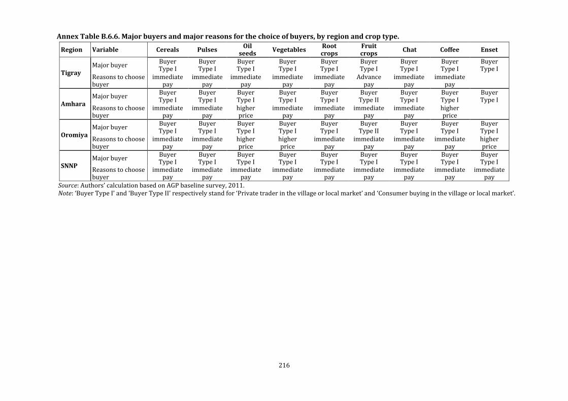
216
Annex Table B.6.6. Major buyers and major reasons for the choice of buyers, by region and crop type.
Region Variable Cereals Pulses Oil
seeds Vegetables
Root crops
Fruit crops
Chat Coffee Enset
Tigray Major buyer
Buyer Type I
Buyer Type I
Buyer Type I
Buyer Type I
Buyer Type I
Buyer Type I
Buyer Type I
Buyer Type I
Buyer Type I
Reasons to choose buyer
immediate pay
immediate pay
immediate pay
immediate pay
immediate pay
Advance pay
immediate pay
immediate pay
Amhara Major buyer
Buyer Type I
Buyer Type I
Buyer Type I
Buyer Type I
Buyer Type I
Buyer Type II
Buyer Type I
Buyer Type I
Buyer Type I
Reasons to choose buyer
immediate pay
immediate pay
higher price
immediate pay
immediate pay
immediate pay
immediate pay
higher price
Oromiya Major buyer
Buyer Type I
Buyer Type I
Buyer Type I
Buyer Type I
Buyer Type I
Buyer Type II
Buyer Type I
Buyer Type I
Buyer Type I
Reasons to choose buyer
immediate pay
immediate pay
higher price
higher price
immediate pay
immediate pay
immediate pay
immediate pay
higher price
SNNP Major buyer
Buyer Type I
Buyer Type I
Buyer Type I
Buyer Type I
Buyer Type I
Buyer Type I
Buyer Type I
Buyer Type I
Buyer Type I
Reasons to choose buyer
immediate pay
immediate pay
immediate pay
immediate pay
immediate pay
immediate pay
immediate pay
immediate pay
immediate pay
Source: Authors’ calculation based on AGP baseline survey, 2011. Note: ‘Buyer Type I’ and ‘Buyer Type II’ respectively stand for ‘Private trader in the village or local market’ and ‘Consumer buying in the village or local market’.

217
Annex B.6.7. Proportion of households that used mobile phone in crop transaction and those that agreed price over mobile phone, if used, by region and crop type
Region Variable Cereals Pulses Oil
seeds Vege
tables Root crops
Fruit crops
Chat Coffee Enset
Tigray Mobile use in crop sale (%) 0.5 0.0 3.0 5.9 6.9 0.0 6.0 0.0
Agreed price over mobile (%) 15.5
92.2 28.6 43.9
0.0
Amhara Mobile use in crop sale (%) 1.2 1.6 0.5 1.9 0.2 0.9 0.0 0.0
Agreed price over mobile (%) 80.2 68.6 100.0 100.0 47.6 0.0
Oromiya Mobile use in crop sale (%) 3.8 3.6 5.3 10.7 4.1 0.0 0.3 2.2 4.3
Agreed price over mobile (%) 94.0 98.0 100 100 63.8
100 100 100
SNNP Mobile use in crop sale (%) 0.6 0.5 0.0 0.0 1.3 0.0 16.8 0.4 2.3
Agreed price over mobile (%) 91.9 17.9 19.3 87.7 100 100
Source: Authors’ calculation based on AGP baseline survey, 2011.
Annex Table B.6.8. Average and proportion of revenue collected from the sale of livestock types, by region
Region Variables Cattle Sheep &
goats Pack
animals Chickens Camels Total
Tigray Average revenue (ETB) 687.8 205.1 23.1 30.6 53.3 1001
Proportion (%) 68.7 20.5 2.3 3.1 5.3 100
Amhara Average revenue (ETB) 741.6 221.8 64.2 24.9 0.9 1053
Proportion (%) 70.4 21.1 6.1 2.4 0.1 100
Oromiya Average revenue (ETB) 1356.4 195.4 83.9 122.5 0.0 1758
Proportion (%) 77.1 11.1 4.8 7.0 0.0 100
SNNP Average revenue (ETB) 834.3 88.7 32.0 6.8 0.0 963
Proportion (%) 86.6 9.2 3.3 0.7 0.0 100
Source: Authors’ calculation based on AGP baseline survey, 2011.
Annex Table B.6.9. Proportion of revenue paid for transportation, by region.
Region Cattle Sheep &
goats Pack animals Chickens
Tigray 0.0 0.0 0.0 0.0
Amhara 0.0 0.2 - 0.1
Oromiya 0.4 0.3 0.0 0.7
SNNP 0.3 0.4 0.5 0.3
Source: Authors’ calculation based on AGP baseline survey, 2011.

218
Annex Table B.6.10. Proportion of households that used mobile phone and that agreed price using mobile, if used, by region
Region Variable Cattle Sheep &
goats Pack
animals Chickens
Tigray Mobile use in sale (%) 1.0 0.0 0.0 0.2
Agreed price over mobile (%) 0.0 100.0
Amhara Mobile use in sale (%) 0.2 0.0 0.5 0.0
Agreed price over mobile (%) 75.9 0.0
Oromiya Mobile use in sale (%) 2.6 0.2 7.7 0.1
Agreed price over mobile (%) 57.5 42.7 51.4 51.4
SNNP Mobile use in sale (%) 0.2 0.2 0.0 0.0
Agreed price over mobile (%) 36.7 46.9
Source: Authors’ calculation based on AGP baseline survey, 2011.
Annex Table B.6.11. Average and proportion of revenue collected from the sale of livestock products, by region
Region Variable Meat Hides
and skins
Butter or
yoghurt
Milk or
cream Dung Eggs Total
Tigray Average Revenue (ETB) 8.6 4.0 41.9 8.1 1.9 34.2 98.7
Proportion (%) 8.7 4.1 42.4 8.2 1.9 34.6 100
Amhara Average Revenue (ETB) 2.7 9.0 19.5 6.3 0.4 39.5 77.3
Proportion (%) 3.4 11.7 25.2 8.1 0.5 51.1 100
Oromiya Average Revenue (ETB) 16.3 7.3 149.2 7.2 2.6 71.9 254.5
Proportion (%) 6.4 2.9 58.6 2.8 1.0 28.2 100
SNNP Average Revenue (ETB) 3.7 2.1 51.4 6.4 0.2 8.5 72.3
Proportion (%) 5.1 2.9 71.1 8.9 0.2 11.7 100
Source: Authors’ calculation based on AGP baseline survey, 2011.
Annex Table B.6.12. Average travel time to the market place and proportion of revenue paid for transportation, by household category and AGP status.
Region Variable Fresh milk Cheese Butter Yoghurt
Tigray Proportion paid for transportation (%) 0.0
0.8
Average travel time to market (minutes) 16.9 0.0 51.0 0.0
Amhara Proportion paid for transportation (%) 0.0
0.0
Average travel time to market (minutes) 25.5 0.0 62.9 0.0
Oromiya Proportion paid for transportation (%) 8.4 4.5 1.0 0.0
Average travel time to market (minutes) 55.1 64.2 73.8 40.0
SNNP Proportion paid for transportation (%) 0.2 1.1 0.5 0.0
Average travel time to market (minutes) 50.3 43.6 50.8 48.6
Source: Authors’ calculation based on AGP baseline survey, 2011.
219
Annex C: Description of Survey Areas based on Community Questionnaire Data
The AGP baseline survey was planned to cover 93 woredas and 305 enumeration areas (EAs)
(see Annex Table A.1.1 above). Two-thirds (62) of the woredas were sampled from among those
included in the AGP program and the remaining 31 from among non-AGP and non-PSNP
woredas. However, the actual data collection comprised 61 AGP woredas and 32 non-AGP/non-
PSNP woredas. Consequently, 200 of the EAs were in AGP woredas while 104 were in non-AGP
woredas. Although households in all 305 EAs were surveyed, the Kebele-level (or community)
survey was conducted in 304 EAs.
In the AGP baseline survey a community is defined as the kebele or peasant association (PA).
Enumerators collected community level data by interviewing at least five people who are
knowledgeable about the community, such as community leaders, PA chairmen, elders, priests,
and teachers. At least one of the five respondents was required to be female and a
representative of the youth was also included in the group of five people. In this section we
describe the surveyed communities using unweighted statistics from data collected. The section
is organized into 6 subsections. In the first subsection we describe the EAs in terms of their
proximity to larger towns, quality, and accessibility of roads. Subsection 2 describes the EAs in
terms of access to tap water, sources of drinking water, and access and coverage quality of
electricity, radio, and mobile phone. The third subsection describes whether or not telephone
centers, post offices, daily and periodic markets, and veterinary service providers are available
in the PA and distances to the nearest center providing such services if it is unavailable in the
PA. In subsection 4 we provide a similar description in terms of elementary, junior, and high
schools and 5 types of health services provision centers: government hospitals, public clinics or
health posts, private clinics, pharmacies, and traditional medical service providers. In
subsection 5 we describe the EAs in terms of timely availability and sufficiency of fertilizer and
improved seeds, and access to and quality of agricultural extension services. In the final
subsection we provide a description of the EAs in terms of access to financial cooperatives
farmers associations, and microfinance institutions.
Proximity to Larger Towns and Roads Quality and Accessibility
Data was collected on names of and distances to large towns closest to the surveyed PAs.
Summary statistics on distances to the nearest towns are provided in columns 3 to 5 of Annex
Table C.1.1. On average, the PAs surveyed are about 14 kilometers (KMs) away from the closest
town while one-half of the PAs were 10 km away. This indicates that EAs with large distances to
nearest towns dominate the mean distance. Among the 304 PAs 10 are located in PAs with

220
relatively larger towns, as a result of which the distance was effectively zero. Distances in the
remaining 294 EAs range from half a kilometer to 100 km. About 40 percent of the EAs are
farther than the mean distance of 14 km, 20 percent are 20 km or more from the nearest town,
10 percent 27 km or more, while 2 percent are 50 km or farther than the nearest town.
Average distance and variation of distances to the nearest town is larger in AGP EAs relatively to
non-AGP EAs. This pattern in average distances and its variation observed in the overall sample
holds true when comparing AGP and non-AGP EAs in the 4 regions with the exception of
Oromiya, in which average distance is smaller in AGP woredas. Relative to the national average,
mean and median distances are larger in an average EA in Tigray and Amhara while they are
smaller in Oromiya and SNNP. The mean distance to the closest town in the 30 AGP EAs in
Amhara is more than twice the mean distance for the 30 non-AGP EAs of SNNP.
The community survey instrument comprised questions on the three most important roads
linking the village to towns in different directions. Data on materials from which the roads are
made of and how well accessible the roads are during rainy and dry seasons are collected.
Accessibility is assessed in terms of means of transport that can be used. Responses to these
questions were obtained for 292 of the 304 EAs while they were not obtained for 6 AGP and 6
non-AGP EAs. The last 4 columns of Table C. 1.1 summarize the materials from which the first
most important roads are made while Table C.1.2 contains summary on the latter 2 questions.
We will also briefly summarize data collected from 182 and 98 EAs on second and third
important roads, respectively.
A large majority of the roads in the EAs surveyed were dirt tracked at 56 percent and accessible
only on foot during rainy seasons. Roads made of stones are second in importance in an average
EA and across AGP and non-AGP EAs, as well as in the corresponding regional subsamples, with
some exceptions. The exceptions to this are: in an average and AGP EAs of Tigray roads made of
concrete are more important, and in an average and non-AGP EAs in Amhara roads made of
other materials are more important. On average, roads made of concrete/tarmac are last in
importance at 11 percent. This held across AGP and non-AGP EAs of the overall sample and in
all 3 categories of the 4 regions, with some exceptions. The exceptions are: in non-AGP woredas
of Oromiya roads made of concrete/tarmac are third in importance, and in non-AGP EAs of
Tigray and in AGP EAs of SNNP they are as much important as roads made of other materials.

221
Annex Table C.1.1. Distance to the nearest town and type of first important road, by region and AGP status.
Region Category
Distance to nearest large town (KMs)
First important road made of (%)
Mean Median SD Concrete Stones Dirt Others
National
All woredas 13.9 10 12.2 11.0 18.8 55.8 14.4
AGP woredas 14.4 10 13.7 13.4 21.6 49.0 16.0
Non-AGP woredas 12.7 10 8.5 6.1 13.3 69.4 11.2
Tigray
All woredas 15.7 14 11.6 16.7 3.3 73.3 6.7
AGP woredas 16.0 14 13.0 22.0 0.0 70.7 7.3
Non-AGP woredas 14.9 14 7.9 5.3 10.5 78.9 5.3
Amhara
All woredas 16.6 12 12.3 5.6 22.2 48.6 23.6
AGP woredas 17.1 12 13.2 8.0 28.0 40.0 24.0
Non-AGP woredas 15.5 14 10.2 0.0 9.1 68.2 22.7
Oromiya
All woredas 12.6 10 9.7 13.9 26.6 43.0 16.5
AGP woredas 12.2 10 10.4 13.5 30.8 36.5 19.2
Non-AGP woredas 13.4 12 8.2 14.8 18.5 55.6 11.1
SNNP
All woredas 11.1 7 14.1 8.6 19.8 61.7 9.9
AGP woredas 12.7 8 17.1 11.8 23.5 52.9 11.8
Non-AGP woredas 8.2 7 5.5 3.3 13.3 76.7 6.7
Source: Authors’ calculations using data from the AGP Baseline Survey, 2011.
In an average EA with data on second important roads, the large majority (51 percent) are dirt
tracks and the proportion of roads made of stones is second largest and this pattern holds in
AGP and non-AGP EAs. Roads made of concrete/tarmac are third in importance in an average
and AGP EAs while concrete/tarmac roads are least in importance in non-AGP EAs. The pattern
observed in the overall sample of EAs about which materials second important roads made of
holds across regions and their AGP-non-AGP subsamples. However, there are more exceptions
in the case of the second important road than in the first. Just to highlight the case, despite the
importance of dirt tracked roads in the 3 categories of the overall sample of EAs, in Oromiya the
proportion of roads made of stones is larger than those that are dirt tracked. Similarly, although
roads made of stones are second in importance in the 3 categories of the overall sample this
holds true in only non-AGP EAs of Tigray and in the 3 categories of SNNP.
In the 82 EAs from which information about the third important roads was elicited, 48 percent
are made of dirt tracks and roads made of stones are second in importance at 22.4 percent.
Roads made of concrete/tarmac are least important at 12 percent in both the overall and AGP
EAs while in non-AGP EAs an equal proportion of roads are made of tarmac/concrete and other
materials.

222
A large majority of 47.4 percent of the roads in an average EA are accessible only on foot during
rainy seasons and the pattern holds in all other categories, with only one category excepted
(Table C.1.2). The exception is that a relatively larger proportion of roads are accessible during
rainy seasons to any vehicle in AGP EAs of Tigray, although the proportion accessible on foot is a
close second. This is despite the proportion of dirt roads in AGP EAs of Tigray is the largest
relative to an average, AGP, and non-AGP EAs of all other regions (excepting non-AGP EAs of the
same region and that of SNNP).
Annex Table C.1.2. Accessibility of the first most important road, by region and AGP status.
Region Category
Accessibility of first important road during rainy season (%)
Accessibility of first important road during dry season (%)
Any vehicle
Trucks and
buses
Mini-bus
Carts or animals
Only walking
Any vehicle
Trucks and
buses
Mini-bus
Carts or animals
Only walking
National
All woredas 30.6 6.2 2.4 13.4 47.4 45.9 7.9 8.9 10.3 27.1
AGP woredas 34.4 5.7 2.6 13.0 44.3 50.5 6.8 7.8 9.4 25.5
Non-AGP woredas 23.2 7.1 2.0 14.1 53.5 37.0 10.0 11.0 12.0 30.0
Tigray
All woredas 38.6 10.5 7.0 3.5 40.4 58.6 12.1 17.2 0.0 12.1
AGP woredas 44.7 5.3 7.9 2.6 39.5 64.1 10.3 12.8 0.0 12.8
Non-AGP woredas 26.3 21.1 5.3 5.3 42.1 47.4 15.8 26.3 0.0 10.5
Amhara
All woredas 31.1 1.4 1.4 8.1 58.1 51.4 5.4 8.1 6.8 28.4
AGP woredas 38.0 2.0 2.0 8.0 50.0 60.0 4.0 6.0 4.0 26.0
Non-AGP woredas 16.7 0.0 0.0 8.3 75.0 33.3 8.3 12.5 12.5 33.3
Oromiya
All woredas 35.0 8.8 0.0 16.3 40.0 38.8 10.0 0.0 18.8 32.5
AGP woredas 37.7 9.4 0.0 13.2 39.6 43.4 7.5 0.0 17.0 32.1
Non-AGP woredas 29.6 7.4 0.0 22.2 40.7 29.6 14.8 0.0 22.2 33.3
SNNP
All woredas 20.0 5.0 2.5 22.5 50.0 38.8 5.0 12.5 12.5 31.3
AGP woredas 19.6 5.9 2.0 25.5 47.1 38.0 6.0 14.0 14.0 28.0
Non-AGP woredas 20.7 3.4 3.4 17.2 55.2 40.0 3.3 10.0 10.0 36.7
Source: Authors’ calculations using data from the AGP Baseline Survey 2011.
The proportion of roads that are accessible to any vehicle during rainy seasons is second in
importance at about 31 percent. This pattern holds in AGP and non-AGP categories of the
overall sample and in all 3 categories of the 4 regions, with 3 categories excepted. The
exceptions are: AGP EAs of Tigray, and average and AGP EAs of SNNP, for which the proportion
accessible to any vehicle is third in importance next to those accessible to carts or animals. By
contrast the proportion accessible to carts or animals is third largest in the 3 categories of the
overall sample, Amhara, and Oromiya, and in non-AGP EAs of SNNP. Roads accessible to trucks
and buses during rainy seasons are fourth in importance in all categories, with the exception of
average and non-AGP EAs in Tigray, for which it is third in importance. The proportion of roads
accessible to mini-buses during rainy seasons is the least important in the 3 categories of the
overall sample as well as in average and AGP EAs of SNNP. The proportion accessible to mini-

223
buses is as much important as those accessible to trucks and buses in the 3 categories of
Amhara and in non-AGP EAs of SNNP. In Tigray, roads accessible to mini-buses are fourth in
importance for average and non-AGP EAs while it is third in importance in AGP EAs.
At an average value of 46 percent, the large majority of the roads are accessible to any vehicle
during dry seasons. This holds also in average, AGP, and non-AGP EAs of all regions, with only 2
exceptions. The exceptions to this are non-AGP EAs of Amhara, in which the proportion is the
same with those suitable for only walking, and in non-AGP EAs of Oromiya, in which the largest
proportion are accessible only on foot even during dry seasons. Particularly, the pattern in
accessibility of roads in non-AGP EAs of Oromiya is the same in both rainy and dry seasons.
The proportion accessible only on foot during dry seasons is second largest in an average EA of
the overall sample, Amhara, Oromiya, and SNNP; and in AGP EAs of the overall sample and all 4
regions, and in non-AGP EAs of the overall sample and SNNP. The proportion of roads accessible
to carts or animals is third largest in all 3 categories of the overall sample and in Oromiya while
it is equally important as those accessible to mini-buses in all 3 categories of SNNP and in non-
AGP EAs of Amhara. In an average and AGP EAs of Amhara roads accessible to carts or animals
is fourth in importance while it is least in importance in all 3 categories of Tigray. Although
roads accessible to mini-buses during dry seasons are fourth in importance in the aggregate
sample they are not so in all of the regions. The proportion accessible to mini-buses is second in
importance across all 3 categories of Tigray, third in importance for an average and AGP EAs of
Amhara, and least in importance in all 3 categories of Oromiya. Roads accessible to trucks and
buses in dry seasons are least in importance in the aggregate sample, in all 3 categories of SNNP,
and in average and non-AGP EAs of Amhara.
Sources of Drinking Water and Access to Electricity, Radio, and Mobile Phone
In this section we describe community data on access to public or private piped water and most
important sources of drinking water (Table C.1.3) and access to and coverage quality of
electricity, cell phone, and radio (Table C.1.4). Accordingly, (public) piped water is available in
110 (36 percent) of the 304 EAs with slightly better access in non-AGP EAs. Relative to average
and AGP EAs in Amhara a significantly large proportion of non-AGP EAs have access to piped
water. The latter has resulted in the relatively better access of non-AGP EAs nationally, given
that AGP EAs have relatively better access in all other regions. Regionally, a significantly larger
proportion of EAs in Tigray and a slightly larger proportion in Amhara have access to piped
water, relative to an average EA in the overall sample.

224
Although 36 percent of the EAs have access to piped water it serves as the most important
source of drinking water for only about 22 percent of the EAs during dry seasons. During dry
season piped water is the third most important source of drinking water, next to springs and
rivers, while wells (boreholes) are fourth in importance, and lakes and other sources are least in
importance. The only exception to the latter is that tap water is more important than rivers in
non-AGP EAs. At 45 percent the largest proportion of EAs in Tigray get their drinking water
from pipes during dry seasons, making Tigray best performing in tap water. The proportion of
EAs that obtain most of their drinking water from piped sources is lower in the 3 categories of
all other regions, relative to their national counterparts. The two exceptions are the slightly
larger proportion of non-AGP EAs in Amhara and AGP EAs in Oromiya.
Respondents were also asked to list second, third, and fourth important sources of drinking
water, if they use them. All 304 EAs listed the second important source. Rivers are the second
important source of drinking water for a largest proportion of EAs at 33 percent closely
followed by those using springs at about 31 percent. The proportion of EAs using piped water as
their second important source of drinking water is the third largest, while those using wells and
lakes and other are fourth and fifth largest, respectively. The pattern observed in the aggregated
sample holds in Amhara with the exception that the proportion using springs is larger than
those using rivers. Similarly the pattern in the aggregate sample holds in Oromiya and SNNP,
with the exception that the proportion using wells is larger than those using tap water in both
regions and the proportion using springs is larger than those using rivers in SNNP.
The second largest proportion of EAs use wells (boreholes) as their second important source of
drinking water in Tigray during dry seasons, next to piped water. Springs, rivers, and lakes and
other sources are third to fifth as the second important source of drinking water in Tigray. A
largest and second largest proportion of EAs use springs and rivers as their second important
source of drinking water in all 3 categories of Amhara, Oromiya, and SNNP, with the exception
that those using tap water is larger in non-AGP EAs of Amhara. The proportion of EAs that use
wells, piped water, and lakes and other sources as their most important source of drinking
water is third to fifth largest in Amhara. In Oromiya and SNNP the proportion using tap water,
wells, and lakes and others as their most important source of drinking water is third to fifth
largest.

225
Annex Table C.1.3. Tap water access and sources of drinking water, by region and AGP status.
Region Woreda
Propor tion with access to
tap water
(%)
First important sources of drinking water during dry seasons (%)
Second important source of drinking water during dry seasons
(%)
Tap water
Wells/ bore holes
Spring River Lakes
and others
Tap water
Wells/ bore holes
Spring River Lakes
and others
National
All woredas 36.2 21.7 12.8 39.8 23.7 2.0 17.8 13.8 30.6 33.2 4.6
AGP woredas 35.5 20.0 12.0 40.0 25.5 2.5 15.5 13.0 32.5 35.5 3.5
Non-AGP woredas 37.5 25.0 14.4 39.4 20.2 1.0 22.1 15.4 26.9 28.8 6.7
Tigray
All woredas 54.8 45.2 27.4 17.7 8.1 1.6 37.1 21.0 17.7 22.6 1.6
AGP woredas 57.1 45.2 23.8 21.4 7.1 2.4 38.1 19.0 16.7 23.8 2.4
Non-AGP woredas 50.0 45.0 35.0 10.0 10.0 0.0 35.0 25.0 20.0 20.0 0.0
Amhara
All woredas 38.8 17.5 18.8 37.5 22.5 3.8 21.3 13.8 32.5 30.0 2.5
AGP woredas 30.2 11.3 20.8 35.8 26.4 5.7 15.1 15.1 39.6 28.3 1.9
Non-AGP woredas 55.6 29.6 14.8 40.7 14.8 0.0 33.3 11.1 18.5 33.3 3.7
Oromiya
All woredas 27.2 16.0 6.2 46.9 29.6 1.2 11.1 12.3 28.4 39.5 8.6
AGP woredas 29.6 20.4 3.7 42.6 33.3 0.0 9.3 11.1 22.2 50.0 7.4
Non-AGP woredas 22.2 7.4 11.1 55.6 22.2 3.7 14.8 14.8 40.7 18.5 11.1
SNNP
All woredas 28.4 13.6 2.5 51.9 30.9 1.2 6.2 9.9 40.7 38.3 4.9
AGP woredas 29.4 7.8 2.0 56.9 31.4 2.0 3.9 7.8 49.0 37.3 2.0
Non-AGP woredas 26.7 23.3 3.3 43.3 30.0 0.0 10.0 13.3 26.7 40.0 10.0
Source: Authors’ calculations using data from the AGP Baseline Survey 2011.
About 19 percent of the 304 EAs have access to electricity services with better access to
electricity in AGP EAs. All 3 categories of EAs in Tigray and average and AGP EAs in Amhara
have better access to electricity, relative to their national counterparts. Access to electricity is
poorer in non-AGP EAs in Amhara, and in all 3 categories of EAs in Oromiya and SNNP, relative
to their national counterparts. Out of the 57 EAs with access to electricity in only 13 (23
percent) is the services excellent (available all the time) or good (available most of the time). In
23 of the EAs (40.4 percent) the services are fair (available about half the time), while in 21 of
the EAs (37 percent) services are poor (available less than half the time) or erratic (rarely
available). In a large proportion of the EAs in Tigray, i.e. 39 percent, electricity services are
excellent or good followed by poor or erratic services, at 33 percent. In Amhara, electricity
services are fair for the largest proportion followed by poor or erratic services, which is about
the same in Oromiya. For an average EA in SNNP about the same proportion of EAs have fair and
poor or erratic electricity services. All non-AGP EAs of SNNP have fair electricity services while
in AGP EAs of SNNP services are fair to a third of the EAs and poor or erratic for two-thirds.
Most notable in SNNP is that in none of the EAs services are excellent or good.

226
Annex Table C.1.4. Electricity, cell phone, and radio - access and quality of services, by region and AGP status.
Region Woreda
Access and reliability of electricity
Access and quality of cell phone cover (%)
Access and quality of radio broadcasts (%)
Propor tion with
access (%)
Excellent or good
Fair Poor or erratic
Propor tion with
access (%)
Excellent or good
Fair Poor or erratic
Propor tion with
access (%)
Excellent or good
Fair Poor or erratic
National
All woredas 18.8 22.8 40.4 36.8 73.0 22.1 37.4 40.5 96.7 62.9 27.9 9.2
AGP woredas
20.0 22.5 37.5 40.0 73.5 19.0 40.8 40.1 96.5 66.3 27.5 6.2
Non-AGP woredas
16.3 23.5 47.1 29.4 72.1 28.0 30.7 41.3 97.1 56.4 28.7 14.9
Tigray
All woredas 29.0 38.9 27.8 33.3 69.4 32.6 39.5 27.9 98.4 73.8 23.0 3.3
AGP woredas
23.8 40.0 30.0 30.0 73.8 25.8 45.2 29.0 100.0 73.8 23.8 2.4
Non-AGP woredas
40.0 37.5 25.0 37.5 60.0 50.0 25.0 25.0 95.0 73.7 21.1 5.3
Amhara
All woredas 22.5 16.7 44.4 38.9 80.0 25.0 32.8 42.2 97.5 66.7 19.2 14.1
AGP woredas
26.4 14.3 35.7 50.0 73.6 23.1 35.9 41.0 98.1 73.1 17.3 9.6
Non-AGP woredas
14.8 25.0 75.0 0.0 92.6 28.0 28.0 44.0 96.3 53.8 23.1 23.1
Oromiya
All woredas 16.0 23.1 46.2 30.8 87.7 11.3 39.4 49.3 96.3 59.0 35.9 5.1
AGP woredas
18.5 30.0 50.0 20.0 83.3 11.1 37.8 51.1 94.4 64.7 33.3 2.0
Non-AGP woredas
11.1 0.0 33.3 66.7 96.3 11.5 42.3 46.2 100.0 48.1 40.7 11.1
SNNP
All woredas 9.9 0.0 50.0 50.0 54.3 25.0 38.6 36.4 95.1 54.5 32.5 13.0
AGP woredas
11.8 0.0 33.3 66.7 62.7 18.8 46.9 34.4 94.1 54.2 35.4 10.4
Non-AGP woredas
6.7 0.0 100 0.0 40.0 41.7 16.7 41.7 96.7 55.2 27.6 17.2
Source: Authors’ calculations using data from the AGP Baseline Survey 2011.
Out of the 304 EAs, 222 or 73 percent have cell phone coverage. Out of the EAs with cell phone
coverage the signals in a largest proportion of 40.5 percent is poor or erratic, it is fair in 37.4
percent, and excellent or good in 22 percent. The pattern in the overall sample holds in non-AGP
EAs while a slightly larger proportion in AGP EAs receive fair signals than those receiving poor
or erratic signals. The pattern observed for an average EA holds in all 3 categories of Amhara
and Oromiya. The proportion of EAs receiving fair signals is larger than those receiving poor or
erratic signals in average and AGP EAs of SNNP while in non-AGP EAs of SNNP an equally large
proportion receive excellent or good and poor or erratic signals. For an average EA in Tigray the
proportion receiving fair and excellent or good signals is largest and second largest,
respectively, while the order is fair and poor or erratic in AGP EAs, and in non-AGP EAs the
proportion receiving excellent or good signals is the largest while the other two are equally
important.

227
Radio broadcasts or signals are received in 294 (about 97 percent) of the EAs, out of this total
185 (63 percent) receive excellent or good signals, in 82 EAs (28 percent) the signals are fair,
while in only 27 (9 percent) the signals are poor or erratic. Not only are the proportion of AGP
and non-AGP EAs with radio signals about the same at 97 percent, but also most categories are
close in the proportion of EAs receiving radio signals, ranging in the narrow band of 94.1 to 100.
Moreover, the pattern in quality of radio signals observed in the overall sample holds in all
other categories.
Access to Social Services, Markets, and Veterinary Services
In this section we describe data collected on whether or not public telephone centers, post
offices, daily markets, periodic markets (that open at least once per week), and veterinary
services are available in the PA and distances to the nearest center out of the PA providing such
services if unavailable in the PA. Summary results of the data are provided in Table C.1.5.
While 34 percent of the EAs have one telephone center in the PA, 4.6 percent have two or more
telephone centers; implying 61.4 percent do not have telephone centers in their respective PAs.
Relative to an average, AGP, and non-AGP EAs nationally, a larger proportion in Tigray have at
least one telephone center while a lower proportion in Oromiya and SNNP have such services.
Average and AGP EAs in Amhara perform worse than their national counterpart while non-AGP
Amhara EAs perform better. Residents of the 187 EAs that do not have telephone centers, on
average, travel 14.7 km while the median distance is 12 km. Distances travelled to telephone
centers range between the lowest averages of 10.2 km in non-AGP EAs of SNNP to 21.8 km in
non-AGP EAs of Amhara.
Only 23 of the 304 EAs (7.6 percent) have a post office in the PA, with non-AGP EAs performing
slightly better. The only region with all 3 subgroups performing better in access to post offices is
SNNP; particularly, non-AGP EAs of SNNP have a rather large proportion of 20 percent. All 3
categories of Amhara and Oromiya perform worse relative to their national counterparts. While
average and AGP EAs in Tigray perform better than their national counterpart, non-AGP EAs in
Tigray perform worse. While residents of EAs with no post offices on average travel 25 km to
the nearest post office out of the Pas, the median distance is 18 km. Surprisingly, in SNNP
(which performs better in terms of presence of post office in the PAs), residents of EAs with no
post office travel the longest relative to their national and regional counterparts. Distance to the
nearest post office out of the PA ranged between averages of 20.7 km in AGP EAs of Oromiya to
34.5 km in non-AGP EAs of SNNP.

228
Only 14.3 percent of the EAs have daily markets within the PA. This averaged about 8 percent in
Tigray and Oromiya, both of which perform worse in all 3 categories relative the corresponding
nationwide categories, while the average is about 20 percent in Amhara and SNNP, both of
which perform better in all 3 categories relative the corresponding national averages. The
average distance to the nearest daily market out of the PA is 21.5 km and it was lower in AGP
EAs. Although a larger proportion of EAs in Amhara and SNNP have daily markets, distances
travelled by residents of average and non-AGP EAs with no markets is larger than the
corresponding national average. With the exception of residents of non-AGP EAs of Tigray, those
with no daily markets in Tigray travel longer than their national counterparts. Although the
proportion of EAs with daily markets is the smallest in Oromiya residents of EAs with no daily
markets travel the shortest average distance of about 15 km.
Relative to the proportion with daily markets, a significantly larger proportion of 48 percent
have periodic markets that open at least once per week with AGP EAs performing better. This
aside the general pattern observed in daily markets almost repeats: a larger proportion of EAs
in Amhara and SNNP have periodic markets and a lower proportion of EAs in Oromiya and
Tigray have periodic markets. The exception relative to daily markets is that a larger proportion
of non-AGP Tigray EAs have periodic markets. Residents of EAs in which periodic markets are
not available travel about 12 km to the nearest market out of the PA, with AGP EAs travelling
less, and the median distance is 9 km. Relative to the 3 national subsamples, residents in an
average EA in Tigray and SNNP and AGP EAs of Tigray and non-AGP EAs of SNNP travel longer
while residents in all 3 categories of Amhara and Oromiya travel shorter.
About 32 percent of the EAs have one or more veterinary service providers with AGP EAs
performing better. Average and non-AGP EAs of Tigray have lower access to veterinary services
than their national counterparts. All 3 categories of Amhara perform better relative to the
corresponding national categories in access to veterinary services while all 3 categories of
Oromiya and average and AGP EAs of SNNP perform worse. Residents of EAs with no veterinary
services on average travel about 15 km with residents AGP EAs travelling less. Residents of
average and non-AGP EAs of Tigray and Amhara travel less relative to their national
counterparts. Residents of all 3 categories of Oromiya and SNNP where there are no veterinary
services travel shorter and longer, respectively, relative to their national counterparts.

229
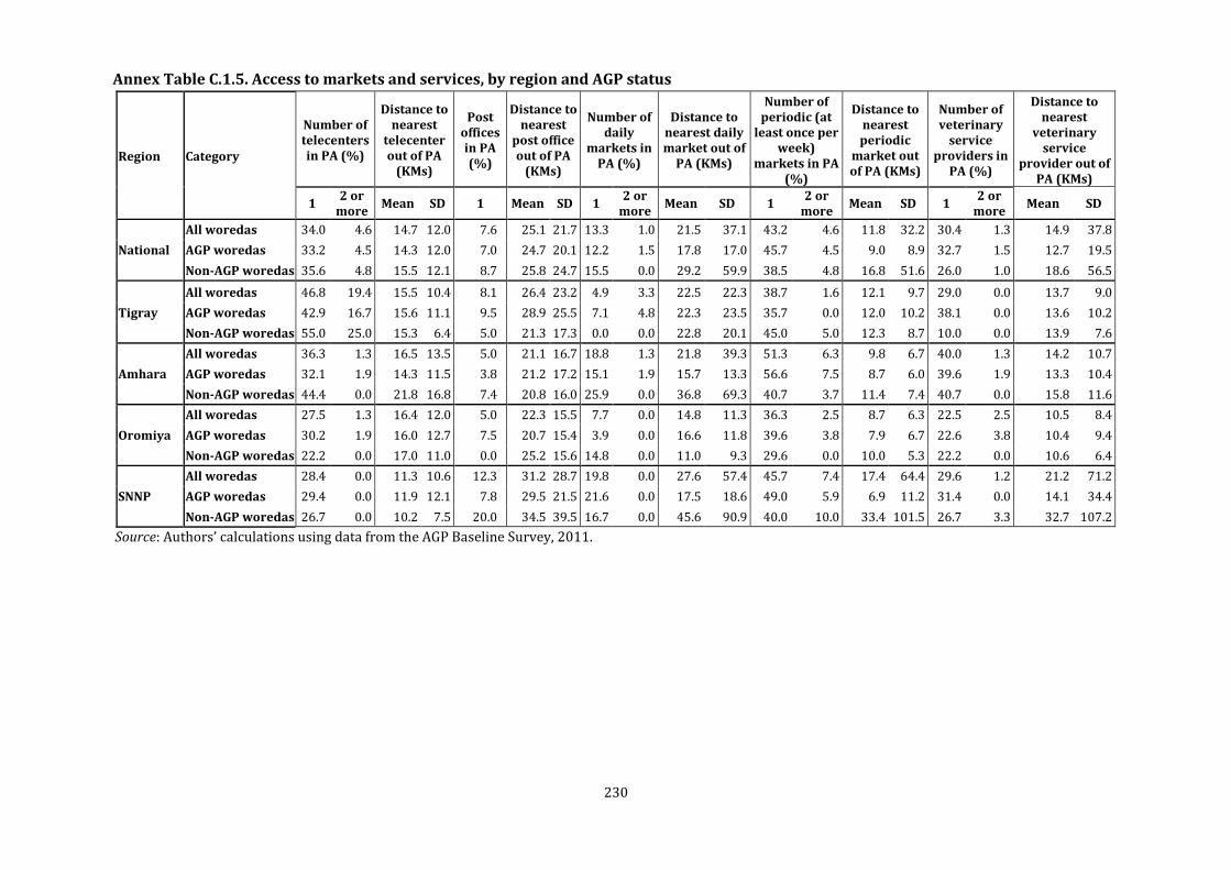
230
Annex Table C.1.5. Access to markets and services, by region and AGP status
Region Category
Number of telecenters in PA (%)
Distance to nearest
telecenter out of PA
(KMs)
Post offices in PA (%)
Distance to nearest
post office out of PA
(KMs)
Number of daily
markets in PA (%)
Distance to nearest daily market out of
PA (KMs)
Number of periodic (at
least once per week)
markets in PA (%)
Distance to nearest periodic
market out of PA (KMs)
Number of veterinary
service providers in
PA (%)
Distance to nearest
veterinary service
provider out of PA (KMs)
1 2 or
more Mean SD 1 Mean SD 1
2 or more
Mean SD 1 2 or
more Mean SD 1
2 or more
Mean SD
National
All woredas 34.0 4.6 14.7 12.0 7.6 25.1 21.7 13.3 1.0 21.5 37.1 43.2 4.6 11.8 32.2 30.4 1.3 14.9 37.8
AGP woredas 33.2 4.5 14.3 12.0 7.0 24.7 20.1 12.2 1.5 17.8 17.0 45.7 4.5 9.0 8.9 32.7 1.5 12.7 19.5
Non-AGP woredas 35.6 4.8 15.5 12.1 8.7 25.8 24.7 15.5 0.0 29.2 59.9 38.5 4.8 16.8 51.6 26.0 1.0 18.6 56.5
Tigray
All woredas 46.8 19.4 15.5 10.4 8.1 26.4 23.2 4.9 3.3 22.5 22.3 38.7 1.6 12.1 9.7 29.0 0.0 13.7 9.0
AGP woredas 42.9 16.7 15.6 11.1 9.5 28.9 25.5 7.1 4.8 22.3 23.5 35.7 0.0 12.0 10.2 38.1 0.0 13.6 10.2
Non-AGP woredas 55.0 25.0 15.3 6.4 5.0 21.3 17.3 0.0 0.0 22.8 20.1 45.0 5.0 12.3 8.7 10.0 0.0 13.9 7.6
Amhara
All woredas 36.3 1.3 16.5 13.5 5.0 21.1 16.7 18.8 1.3 21.8 39.3 51.3 6.3 9.8 6.7 40.0 1.3 14.2 10.7
AGP woredas 32.1 1.9 14.3 11.5 3.8 21.2 17.2 15.1 1.9 15.7 13.3 56.6 7.5 8.7 6.0 39.6 1.9 13.3 10.4
Non-AGP woredas 44.4 0.0 21.8 16.8 7.4 20.8 16.0 25.9 0.0 36.8 69.3 40.7 3.7 11.4 7.4 40.7 0.0 15.8 11.6
Oromiya
All woredas 27.5 1.3 16.4 12.0 5.0 22.3 15.5 7.7 0.0 14.8 11.3 36.3 2.5 8.7 6.3 22.5 2.5 10.5 8.4
AGP woredas 30.2 1.9 16.0 12.7 7.5 20.7 15.4 3.9 0.0 16.6 11.8 39.6 3.8 7.9 6.7 22.6 3.8 10.4 9.4
Non-AGP woredas 22.2 0.0 17.0 11.0 0.0 25.2 15.6 14.8 0.0 11.0 9.3 29.6 0.0 10.0 5.3 22.2 0.0 10.6 6.4
SNNP
All woredas 28.4 0.0 11.3 10.6 12.3 31.2 28.7 19.8 0.0 27.6 57.4 45.7 7.4 17.4 64.4 29.6 1.2 21.2 71.2
AGP woredas 29.4 0.0 11.9 12.1 7.8 29.5 21.5 21.6 0.0 17.5 18.6 49.0 5.9 6.9 11.2 31.4 0.0 14.1 34.4
Non-AGP woredas 26.7 0.0 10.2 7.5 20.0 34.5 39.5 16.7 0.0 45.6 90.9 40.0 10.0 33.4 101.5 26.7 3.3 32.7 107.2
Source: Authors’ calculations using data from the AGP Baseline Survey, 2011.
231
Access to Education and Health Services
Only 5 percent of the surveyed EAs do not have primary schools in their PAs. Out of the 95 EAs
with at least one primary school 62 percent have one, 17 percent have 2, and 16 percent have 3
primary schools. Amhara constitutes a region with universal primary school coverage as do
non-AGP EAs of Tigray. Except for AGP EAs in Oromiya, which have the lowest coverage of 88
percent resulting in an overall average of about 90 percent in Oromiya, the minimum coverage
of primary schools is 93 percent in all other categories. A pupil in an average EA with no
primary school travelled about 4.4 km while students in one-half of the EAs with no primary
school travelled 3 or more km. The distance travelled is slightly longer in AGP EAs. This is
mainly because of a non-AGP EA in Tigray, which is 17 km away from the nearest primary
school. Disregarding this EA the average distance travelled by a student is 3.3 km while the
maximum distance is 6 km.
About 46 percent of the EAs have a junior secondary school (JSS) in the PAs while 5.6 percent
have two junior secondary schools (JSS), with students in 48.5 percent (147) of the EAs that do
not have JSS travelling an average of 12 km to the nearest school. Distances travelled to JSS
range from 0.5 to 70 km, the median distance is 9 km, and students in 10 percent of the EAs
travel 30 to 70 km. Relative to their national counterpart, access to JSS is better in all 3
categories of Amhara, particularly in non-AGP EAs that have JSS coverage about 20 percent
larger than the national non-AGP average of 11.7 percent. Access to JSS is worse in all 3
categories of Tigray and SNNP. Non-AGP EAs in Oromiya perform better while AGP EAs and an
average EA in the region perform worse than their national counterparts. Despite the poor
performance in access to JSS in SNNP, distances travelled by students in all 3 categories of SNNP
are shorter while the opposite holds in Amhara, the region that perform better in access to JSS,
both relative to distances travelled by their national counterparts. Not only perform EAs in all 3
categories in Tigray worse in access to JSS but also students in an average and AGP EAs in
Tigray travel longer relative to students in their national counterparts.

232
Annex Table C.1.6. Number of schools in PAs and distances travelled where unavailable, by region and AGP status
Region Woreda
Proportion with primary schools in PA
(%)
Dist. to nearest primary
school out of PA (KMs)
Proportion with junior
high schools in PA (%)
Dist. to nearest junior high
school out of PA (KMs)
Proportion with one
high school in PA (%)
Dist. to nearest high school out of
PA (KMs)
1 2 or
more Mean SD 1
2 or more
Mean SD
Mean SD
National
All woredas 62.3 33.0 4.4 4.2 45.9 5.6 12.0 11.3 5.6 18.2 16.3
AGP woredas 59.9 35.0 5.1 4.6 41.5 5.5 12.1 12.0 6.0 18.5 16.0
Non-AGP woredas 67.0 29.1 2.3 1.2 54.4 5.8 11.7 9.3 4.8 17.8 16.9
Tigray
All woredas 41.9 56.5 17.0 _ 43.5 16.1 12.9 9.9 6.6 20.1 19.7
AGP woredas 31.0 66.7 17.0 _ 40.5 16.7 13.8 10.2 7.3 21.3 21.6
Non-AGP woredas 65.0 35.0 _ _ 50.0 15.0 9.8 9.5 5.0 17.7 15.8
Amhara
All woredas 46.8 53.2 _ _ 59.5 5.1 16.2 16.0 6.3 19.4 15.7
AGP woredas 49.1 50.9 _ _ 52.8 7.5 15.5 16.6 9.4 19.1 16.6
Non-AGP woredas 42.3 57.7 _ _ 73.1 0.0 18.3 15.1 0.0 19.9 14.2
Oromiya
All woredas 75.6 14.1 3.3 1.5 46.9 3.7 11.7 8.5 3.7 16.5 12.2
AGP woredas 72.5 15.7 3.8 1.3 42.6 0.0 11.9 9.2 3.7 16.7 12.3
Non-AGP woredas 81.5 11.1 2.0 1.4 55.6 11.1 10.9 6.1 3.7 15.9 12.1
SNNP
All woredas 80.2 13.6 3.3 1.3 33.3 0.0 9.6 10.1 6.2 17.5 17.7
AGP woredas 82.4 11.8 3.3 1.5 29.4 0.0 9.3 11.4 3.9 17.6 13.7
Non-AGP woredas 76.7 16.7 3.0 _ 40.0 0.0 10.1 7.4 10.0 17.4 23.7
Source: Authors’ calculations using data from the AGP Baseline Survey, 2011.
Only 17 (about 6 percent) of the EAs have high schools in their PAs. There are 3 high schools in
the 30 non-AGP EAs of SNNP and 5 high schools in the 53 AGP EAs of Amhara, categories which
performed first and second best. There are no high schools in the 27 non-AGP EAs of Amhara,
which performs worst and contrasts to the AGP EAs in the same region. Both AGP and non-AGP
EAs in Oromiya perform worse, next to non-AGP EAs in Amhara, with a ratio of 1 high school in
27 EAs. On average, high school students travel about 18.2 km, which is about 50 percent longer
than distance travelled to junior secondary schools. Distances travelled by high school students
range from 0.5 to 125 km, students in one-half of the EAs travel 14 km or more, students in 20
and 10 percent of the EAs travel 26 and 36 km or more. Relative to the corresponding national
categories, distances travelled by students in all 3 categories of Amhara, in average and AGP EAs
of Tigray are longer, while distances travelled by students in all 3 categories of Oromiya and
SNNP are shorter.
Government hospitals are available in only 8 (2.6 percent) of the 304 EAs. AGP EAs of Amhara,
Oromiya, and SNNP each have a hospital, AGP EAs of Tigray have 2 hospitals and non-AGP EAs
of SNNP, which perform best, have 3 hospitals. Residents of the 296 EAs that do not have

233
hospitals in their PAs travel an average of 56 km to the nearest government hospital for
treatment while the median distance is 45 km. In the national sample, distances travelled by
residents where hospitals are unavailable range from 0.5 to 250 km. Residents in 30 percent of
these EAs travel 72 km or more, residents in 20 percent of the EAs travel 90 km or more, and
residents in the most remote 10 percent EAs travel 120 km or longer to the nearest government
hospital.
Government clinics or health posts are available in 235 (77.3 percent) of the 304 EAs out of
which 15 EAs (about 5 percent) have two such clinics. Non-AGP woredas are endowed with
slightly more government clinics. Relative to the corresponding national average, the
proportion of EAs with at least one government clinic is larger in all 3 categories of Tigray and
SNNP; particularly, non-AGP EAs in Tigray have a markedly higher clinic availability of 95
percent. A lower proportion of EAs in all 3 categories of Oromiya and average and non-AGP EAs
in Amhara have clinics. In 6 of the 26 EAs where government clinics/health posts are not
available there are private clinics. Residents of the 26 EAs in which government clinics are
unavailable travel 11 km to the nearest health clinic out of the PA, with a median distance of 9.2
KMs. Residents in AGP EAs travel 4.5 km longer than those in non-AGP EAs. Residents in
average and AGP EAs of Tigray and Oromiya, and residents in all 3 categories of EAs in SNNP
travel longer than their national counterparts while those in average and AGP EAs of Amhara
travel shorter distances.
There are 62 private clinics operating in 49 of the 304 EAs; that is, there are 36 EAs in which
there is a single private clinic and 13 EAs with 2 private clinics. AGP EAs of Amhara and non-
AGP EAs of SNNP have relatively larger proportion of private clinics with 28 and 21 percent of
the EAs served by at least one private clinic, respectively. By contrast non-AGP and AGP EAs of
Tigray perform worst with at least one private clinic in only 5 and 10 percent of them,
respectively. In the 255 EAs where private clinics are unavailable, residents on average travel
18 km to the nearest such center out of the PA. Distances to the nearest private clinic out of the
PA ranged from 0.5 to 158 km while the median distance is 12 km. Residents in 20 and 10
percent of the EAs travel 24 and 36 km or more, respectively. Relative to the 3 categories of the
overall sample, distances travelled by residents in all 3 categories of EAs in Tigray are longer
and those in the remaining 3 regions are shorter. The only exception to this is non-AGP EAs of
SNNP, where residents travel a kilometer longer than those in the corresponding national
average.

234
Annex Table C.1.7. Access to health facilities in PAs and distances travelled where unavailable, by region and AGP status
Region Category
Prop. with a
gov. hospital
in PA (%)
Dist. to nearest gov. hospital out of PA (km)
Prop. with gov. health clinics/pos
ts in PA (%)
Dist. to nearest gov.
health clinic/ post out of PA
(km)
Prop. with
private clinics in PA (%)
Dist. to nearest private
clinic out of PA (km)
Prop. with
pharmacies in PA (%)
Dist. to nearest
pharmacy out of PA
(km)
Prop. with traditional
medical service
providers in PA (%)
Dist. to nearest traditional
medical service
provider out of PA (km)
Mean SD Mean SD Mean SD Mean SD Mean SD
National
All woredas 2.6 55.8 45.5 77.3 11.0 9.2 16.3 17.8 18.9 10.0 19.0 20.3 15.0 32.0 39.3
AGP woredas 2.5 53.9 45.7 76.5 12.4 10.2 17.7 17.9 21.1 11.6 19.2 22.3 14.9 29.3 37.3
Non-AGP woredas 2.9 59.2 45.1 78.8 7.9 5.5 13.7 17.5 14.3 6.9 18.5 16.4 15.3 37.4 42.9
Tigray
All woredas 3.3 52.4 44.7 85.5 11.6 7.7 8.2 29.1 29.0 16.4 23.2 23.0 31.7 30.4 32.3
AGP woredas 4.9 59.2 50.5 81.0 13.3 6.7 9.8 33.4 34.1 17.1 26.3 26.3 31.7 30.7 33.6
Non-AGP woredas 0.0 39.2 27.4 95.0 0.0 _ 5.0 21.3 13.2 15.0 26.3 26.3 31.6 29.7 30.6
Amhara
All woredas 1.3 74.7 55.7 78.8 9.5 4.8 22.8 15.4 12.7 2.5 22.3 27.1 10.6 30.8 40.4
AGP woredas 1.9 72.1 57.9 84.9 9.8 5.2 28.3 14.4 13.6 3.8 21.9 29.7 9.8 25.4 33.8
Non-AGP woredas 0.0 79.3 52.4 66.7 9.3 4.7 11.5 16.9 11.1 0.0 23.0 22.2 12.5 41.7 50.4
Oromiya
All woredas 1.2 43.4 32.5 65.4 11.1 9.0 17.5 12.4 8.8 8.6 15.0 10.9 8.0 29.6 34.0
AGP woredas 1.9 38.3 29.6 59.3 12.6 9.3 18.9 11.5 9.2 11.1 14.8 11.9 10.4 28.0 32.9
Non-AGP woredas 0.0 53.3 36.1 77.8 5.0 4.2 14.8 14.0 7.9 3.7 15.2 9.1 3.7 32.6 36.5
SNNP
All woredas 4.9 51.8 40.6 81.5 12.4 14.0 15.0 15.7 16.5 14.1 16.1 15.2 13.1 37.0 47.7
AGP woredas 2.0 48.3 35.5 82.4 13.7 17.1 11.8 14.2 13.5 15.7 15.2 13.7 10.4 34.2 47.2
Non-AGP woredas 10.0 58.2 48.6 80.0 10.0 6.8 20.7 18.5 21.3 11.1 17.8 17.8 17.9 43.5 49.6
Source: Authors’ calculations using data from the AGP Baseline Survey, 2011.

235

236
There are 33 pharmacies providing services in 30 EAs, with 3 EAs served by 2 pharmacies. AGP
EAs in Tigray and SNNP perform better in terms of availability of pharmacies with 17 and about
16 percent of the EAs served by at least one pharmacy. By contrast, there are no pharmacies in
non-AGP EAs of Amhara, which do not also have government hospitals that often include
pharmacies as part of their services. Non-AGP EAs in Oromiya and AGP EAs in Amhara have the
next 2 lowest proportions at about 4 percent. Residents of the 274 EAs where pharmacies are
unavailable in their PAs travel 19 km to the nearest pharmacy out of the PA, with the distance
slightly shorter for non-AGP residents. Distances travelled by residents of EAs where
pharmacies are unavailable range from 0.5 to 193 km, the median is 14 km, and residents in 20
percent of the EAs travelled 25 km or more while those in the farthest 10 percent travel 42 km
or more. Distances travelled to pharmacies out of the PA are longer in all 3 categories of EAs in
Tigray and Amhara and shorter in Oromiya and SNNP, relative to corresponding national
averages.
Out of the 304 EAs 29 (10 percent) are served by a single local (cultural) medication center,
while about 5 percent are served by 2 or more local medication centers, ranging up to 8 such
centers in an AGP EA in Tigray. The proportion of EAs served by local medication centers is
generally higher in Tigray with the proportion of EAs in all 3 categories of Tigray about twice
the proportion in average, AGP, and non-AGP EAs of the overall sample as well as in the
remaining 3 regions, with the exception of non-AGP EAs in SNNP. By contrast, all 3 categories of
Amhara, Oromiya, and SNNP have lower proportion of EAs with local medical centers relative to
their national counterparts, again with the exception of non-AGP EAs in SNNP. Distances
travelled to local medical centers average 32 km, the median is 17 km, and it ranges from 0.5 to
210 km. Distances travelled by residents of EAs with no local medical centers is larger than their
national counterparts in all 3 categories of EAs in SNNP, AGP EAs in Tigray, and non-AGP EAs of
Amhara.
Access and Patterns of Distribution of Modern Inputs: Fertilizer, Improved Seeds,
and Extension
In this section we describe data collected in 2 parts of the community survey. The first part
pertains to the timely availability, sufficiency, and distribution criterion of fertilizer and
improved seeds. The second is on availability of extension offices, trends in quality of service
provision, and on the number and qualitative aspects of extension agents. We provide summary
results of the first part in Table C.1.8 and the second part is summarized in Table C.1.9.

237
Out of the 300 EAs that responded to the question enquiring whether or not fertilizer was
available before Meher 77 percent (232) responded in the affirmative. The proportion of EAs
where fertilizer was made available before Meher is larger in all 3 categories of EAs in SNNP, in
average and non-AGP EAs of Tigray, and in AGP EAs in Amhara, relative to their national
counterparts. In about 88 percent of the EAs where fertilizer was made available before Meher
there is enough fertilizer, with a slightly larger proportion of AGP EAs facing fertilizer shortage
at 16 percent. The proportion of EAs with fertilizer shortage is larger in all 3 categories of
Tigray and in average and AGP EAs of SNNP relative to their national counterparts.
Respondents in each EA were asked to name the 3 most important criteria used to allocate
fertilizer among farmers that wanted to use the input. In the largest proportion of EAs (48.5
percent) the ability to pay cash is the most important criterion. In 20 percent of the EAs there
are no priority groups or no criterion was used. Out of the 6 specific criterion listed the ability to
use credit is third in importance, used in 16.5 percent of the EAs. The category of others, which
totaled 17 percent, includes 9.2 percent of the EAs in which the most important criterion used
to allocate fertilizer is the ability to pay the highest price. Included also in the “others” category
is the 4.6 percent of EAs where being approved by a development agent is the most important
criterion and the 3 percent of the EAs where being knowledgeable about fertilizer is the most
important criterion. Among EAs that provided a second criterion the largest proportion of about
37 percent the ability to use credit is the most important criterion followed by the ability to pay
cash, which is used in 31 percent of the EAs. The criterion of approval by a development agent
and being knowledgeable about fertilizer are third and fourth important and are used in about
15 and 10 percent of the EAs, respectively. Approval by a development agent, being
knowledgeable about fertilizer, and ability to buy on credit are first to third important in EAs
that provided 3 criteria.
There are differences in the first most important criterion by AGP classification as well as
among regions. Relative to the criterion in the national average the category of “others” is more
important than no priority group in AGP EAs while the use of credit is more important than
“others” in non-AGP EAs. Taken together, the pattern in average, AGP, and non-AGP EAs of
Tigray is the most dissimilar when compared with that observed nationally while that in
Oromiya is most similar.

238

239
Annex Table C.1.8. Availability, sufficiency, and criteria for allocation of fertilizer and improved seeds, by region and AGP status
Region Category
Fertilizer available
in time for Meher (%)
Sufficient fertilizer available
(%)
Fertilizer allocated to those satisfying the criterion
Improved seeds
available in time for Meher (%)
Sufficient improved
seeds available
(%)
Improved seeds allocated to those satisfying the criterion
Pay cash
Use credit
No priority groups
Others Pay the
highest
Pay cash
Use credit
No priority groups
Others
National
All woredas 77.3 87.8 48.5 14.6 20.0 16.9 54.7 77.2 16.1 40.7 13.6 17.8 11.9
AGP woredas 76.6 83.9 42.7 17.1 18.3 22.0 56.9 72.3 15.7 42.2 13.3 16.9 12.0
Non-AGP woredas 78.6 95.1 58.3 10.4 22.9 8.3 50.5 88.0 17.1 37.1 14.3 20.0 11.4
Tigray
All woredas 81.4 79.2 10.3 27.6 51.7 10.3 66.1 72.5 4.2 8.3 29.2 45.8 12.5
AGP woredas 75.0 73.3 4.5 36.4 45.5 13.6 70.0 62.1 4.8 4.8 33.3 42.9 14.3
Non-AGP woredas 94.7 88.9 28.6 0.0 71.4 0.0 57.9 100.0 0.0 33.3 0.0 66.7 0.0
Amhara
All woredas 72.5 93.0 61.5 7.7 15.4 15.4 45.0 64.7 19.0 42.9 4.8 19.0 14.3
AGP woredas 77.4 92.5 46.7 6.7 26.7 20.0 49.1 61.5 18.8 43.8 0.0 25.0 12.5
Non-AGP woredas 63.0 94.1 81.8 9.1 0.0 9.1 37.0 75.0 20.0 40.0 20.0 0.0 20.0
Oromiya
All woredas 75.3 91.8 76.7 0.0 10.0 13.3 49.4 77.5 12.5 62.5 3.1 9.4 12.5
AGP woredas 75.9 87.8 84.2 0.0 0.0 15.8 55.6 76.7 17.4 69.6 0.0 4.3 8.7
Non-AGP woredas 74.1 100.0 63.6 0.0 27.3 9.1 37.0 80.0 0.0 44.4 11.1 22.2 22.2
SNNP
All woredas 81.3 85.9 46.7 20.0 8.9 24.4 61.3 89.6 24.4 41.5 17.1 7.3 9.8
AGP woredas 78.0 78.9 42.3 19.2 3.8 34.6 56.0 88.9 21.7 47.8 17.4 0.0 13.0
Non-AGP woredas 86.7 96.2 52.6 21.1 15.8 10.5 70.0 90.5 27.8 33.3 16.7 16.7 5.6
Source: Authors’ calculations using data from the AGP Baseline Survey 2011.

240

241
Out of the 300 EAs that provided a reply for the question whether or not improved seeds were
available before Meher 55 percent (164) responded in the affirmative. Improved seeds are
made available in larger proportion of AGP EAs. Availability of improved seeds is relatively
better in all 3 categories of Tigray and in average and non-AGP EAs of SNNP. Among the EAs
where improved seeds were made available before Meher it is sufficient in 77 percent with
farmers in a significantly large proportion of non-AGP EAs able to obtain sufficient improved
seeds. Although average and AGP EAs in Tigray fare worse relative to their national
counterparts, sufficient improved seeds are made available in all non-AGP EAs of Tigray. EAs in
all 3 categories of Amhara perform worse relative to their national counterparts while the
reverse is true in SNNP. An average EA in Oromiya perform slightly better while AGP EAs
perform better, both relative to their national counterparts. Respondents were asked to list the
3 important criteria that were used to allocate improved seeds. For the most part, the pattern in
the importance of the criteria used to allocate improved seeds is similar with those used to
allocate fertilizer.
Government extension or development agent offices are available in the respective PAs of 252
(83 percent) of the 304 EAs. Out of the 52 EAs with no extension office 25 and 8 are in AGP and
non-AGP EAs of SNNP, 10 and 6 are in AGP and non-AGP EAs of Oromiya, 2 in AGP EAs of Tigray,
and 1 in AGP EAs of Amhara. Distances travelled to the nearest extension office out of the PA
average 12 km, range between 1 and 56 km, and farmers in 50 percent of the EAs with no
extension office travel 7.5 km or more to such offices located out of the PA. The distances are
longer in Oromiya and shorter in SNNP relative to the national averages.
In a large majority of 75.4 percent of the EAs extension service provisions have improved in the
2 years before the survey, were about the same in 16.3 percent, and deteriorated in 8.3 percent.
The trend in the quality of extension service provision observed in the recent past in the
aggregated sample holds true in all remaining subcategories.
Not only is there a large presence of extension offices observed but also the proportion of EAs
with 3 or more development agents (DAs) is the largest at 71 percent and this includes 21, 9, 4
and 1 EA with 4, 5, 6, and 9 development agents. Moreover, the proportion of EAs with 2 DAs is
the second largest at 26 percent. The pattern in the number of DAs observed in the aggregate
sample also holds in all other subsamples.
Questions were asked about years of experience and specialization of three extension agents.
The data indicates that in an average EA the first extension agent is relatively more experienced,
which is why we used the data about the first development agent (DA) in Table C.1.9. The

242
largest proportion (90 percent) of the development agents have only 0-5 years of experience
working in the PAs, about 9 percent serve in the PA for 5 to 10 years, and about 1 percent serve
for longer than 10 years. Among the least experienced group of DAs only 5 percent have 0 years
of experience, a largest proportion of 29 percent have at least one year of experience, followed
by those who have 2, 3, 4, and 5 years of experience at 28, 18, 13, and about 7 percent. The
pattern in the number of years of experience observed in the aggregated sample also holds in all
other subsamples with the exception in non-AGP EAs of Oromiya and AGP EAs of SNNP, which
have no DAs with 5-10 years of experience.
In the largest proportion of EAs (41 percent) the first development agent was specialized in
crops, followed by those specialized in non-agricultural income generation activities at 31
percent and in livestock at 25.4 percent. The proportion specialized in crops is largest in all
subcategories with the exception of non-AGP EAs in SNNP in which the proportion of
development agents specialized in non-agricultural income generation activities is the largest
followed by those trained in livestock. While EAs in Tigray and Amhara are mostly similar with
the aggregated sample, in Oromiya the proportion of development agents trained in livestock is
larger than those trained in non-agricultural income generation activities.

243
Annex Table C.1.9. Access to and quality of extension services, by region and AGP status
Region Category
Proportion with
extension office in PA
(%)
Dist. to nearest extension office out of PA (km)
Access to extension services in the last 2 years
(proportion %)
Number of development
agents in extension office
Years of experience development agent 1 in PA (proportion in
%)
Specialty of development agent 1 (proportion in %)
Mean SD Improved Was
same Deteriorated 1 2
3 or more
0 to 5 6 to 10
10 or more
Crops Livestock Non-agri. income
gen. activ. Others
National
All woredas 82.9 12.1 12.8 75.4 16.3 8.3 2.8 26.2 71.0 90.1 9.1 0.8 40.9 25.4 31.0 2.8
AGP woredas 81.0 13.3 14.4 75.3 15.4 9.3 1.2 26.5 72.2 90.1 9.3 0.6 44.4 22.8 29.6 3.1
Non-AGP woredas 86.5 8.8 7.0 75.6 17.8 6.7 5.6 25.6 68.9 90.0 8.9 1.1 34.4 30.0 33.3 2.2
Tigray
All woredas 96.8 8.0 2.8 78.3 16.7 5.0 1.7 6.7 91.7 81.7 18.3 0.0 46.7 25.0 28.3 0.0
AGP woredas 95.2 8.0 2.8 75.0 17.5 7.5 0.0 5.0 95.0 80.0 20.0 0.0 47.5 25.0 27.5 0.0
Non-AGP woredas 100.0 0.0 0.0 85.0 15.0 0.0 5.0 10.0 85.0 85.0 15.0 0.0 45.0 25.0 30.0 0.0
Amhara
All woredas 98.8 4.0 0.0 65.8 19.0 15.2 5.1 34.2 60.8 88.6 11.4 0.0 40.5 19.0 35.4 5.1
AGP woredas 98.1 4.0 0.0 67.3 19.2 13.5 1.9 32.7 65.4 90.4 9.6 0.0 42.3 13.5 38.5 5.8
Non-AGP woredas 100.0 0.0 0.0 63.0 18.5 18.5 11.1 37.0 51.9 85.2 14.8 0.0 37.0 29.6 29.6 3.7
Oromiya
All woredas 80.2 18.0 15.0 70.8 20.0 9.2 3.1 36.9 60.0 95.4 3.1 1.5 38.5 30.8 26.2 4.6
AGP woredas 81.5 23.9 16.5 72.7 15.9 11.4 2.3 36.4 61.4 95.5 4.5 0.0 40.9 29.5 25.0 4.5
Non-AGP woredas 77.8 10.2 8.6 66.7 28.6 4.8 4.8 38.1 57.1 95.2 0.0 4.8 33.3 33.3 28.6 4.8
SNNP
All woredas 59.3 9.2 11.1 93.8 6.3 0.0 0.0 22.9 77.1 95.8 2.1 2.1 37.5 29.2 33.3 0.0
AGP woredas 51.0 9.8 12.4 96.2 3.8 0.0 0.0 30.8 69.2 96.2 0.0 3.8 50.0 26.9 23.1 0.0
Non-AGP woredas 73.3 7.2 4.9 90.9 9.1 0.0 0.0 13.6 86.4 95.5 4.5 0.0 22.7 31.8 45.5 0.0
Source: Authors’ calculations using data from the AGP Baseline Survey, 2011.

244
Financial Cooperatives, Farmers’ Associations, and Micro-Finance Institutions
The community survey included questions about availability of credit and savings cooperatives,
credit and loans cooperatives, peasant associations, and small microfinance institutions. The
questions include the number of such institutions in the PA, distances to the nearest outside the PA
if unavailable, and services provided by such institutions. We summarize the data on each of the
institutions in Tables C.1.10 through C.1.13.
In 40.5 percent of the EAs there is at least one saving and credit cooperative (SCC). Relative to their
national counterparts EAs in all 3 categories of Tigray have better access to SCCs, particularly the
proportion of average and non-AGP EAs where the access to SCCs is about twice as large. Non-AGP
EAs in Oromiya are the only other category that performs better. A large majority of the EAs that
have SCCs have only one such cooperative and this is true in all subcategories. In EAs where there
are no saving and credit cooperatives in the PA the closest SCC is located at an average distance of
18 km. The distance is longer in an average EA of Tigray and Amhara while the reverse is true in
Oromiya and SNNP.
A large proportion of the SCCs (52 percent) provide credit, followed closely by those who provide
agricultural credit at 50.4 percent, while 48.4 percent of the SCCs sold improved/hybrid seeds.
Relative to their national counterparts a larger proportion of saving and credit cooperatives in
Tigray and Amhara provide all 3 services while the reverse holds true in Oromiya and SNNP. In
most, 96 percent, of the EAs there are restrictions on membership and that ranges from 80 percent
in non-AGP EAs of Oromiya to 100 percent in all 3 categories of Tigray, and non-AGP EAs of Amhara
and SNNP.

245
Annex Table C.1.10. Distribution of saving and credit cooperatives (SCCs) and services they provided, by region and AGP status.
Region Category
Propor tion with
SCCs in PA (%)
Number of SCCs in PA
(%)
Distance to the nearest SCC out of
PA (km)
Services provided by the SCCs before the recent Meher season
(%)
Proportion with
restrictions to be a
member (%)
1 2 or
more Mean SD
Sold fertilizer
Sold improved/
hybrid seeds
Provided agricultural
credit
National
All woredas 40.5 78.0 22.0 18.0 15.9 52.0 48.4 50.4 95.9
AGP woredas 43.0 79.1 20.9 19.8 18.2 52.3 49.4 54.7 96.5
Non-AGP woredas 35.6 75.7 24.3 14.8 9.8 51.4 45.9 40.5 94.6
Tigray
All woredas 80.6 76.0 24.0 25.6 36.0 74.0 68.0 74.0 100
AGP woredas 78.6 78.8 21.2 29.3 37.9 72.7 63.6 75.8 100
Non-AGP woredas 85.0 70.6 29.4 3.0 0.0 76.5 76.5 70.6 100
Amhara
All woredas 30.0 91.7 8.3 22.3 15.8 66.7 62.5 62.5 95.8
AGP woredas 37.7 90.0 10.0 23.4 19.3 65.0 65.0 65.0 95.0
Non-AGP woredas 14.8 100.0 0.0 20.9 10.0 75.0 50.0 50.0 100
Oromiya
All woredas 34.6 67.9 32.1 16.9 11.7 25.0 21.4 28.6 89.3
AGP woredas 33.3 66.7 33.3 17.5 13.2 33.3 27.8 38.9 94.4
Non-AGP woredas 37.0 70.0 30.0 15.7 8.6 10.0 10.0 10.0 80.0
SNNP
All woredas 25.9 81.0 19.0 14.8 13.5 19.0 20.0 9.5 95.2
AGP woredas 29.4 80.0 20.0 17.5 15.1 13.3 21.4 13.3 93.3
Non-AGP woredas 20.0 83.3 16.7 9.7 7.9 33.3 16.7 0.0 100
Source: Authors’ calculations using data from the AGP Baseline Survey, 2011.
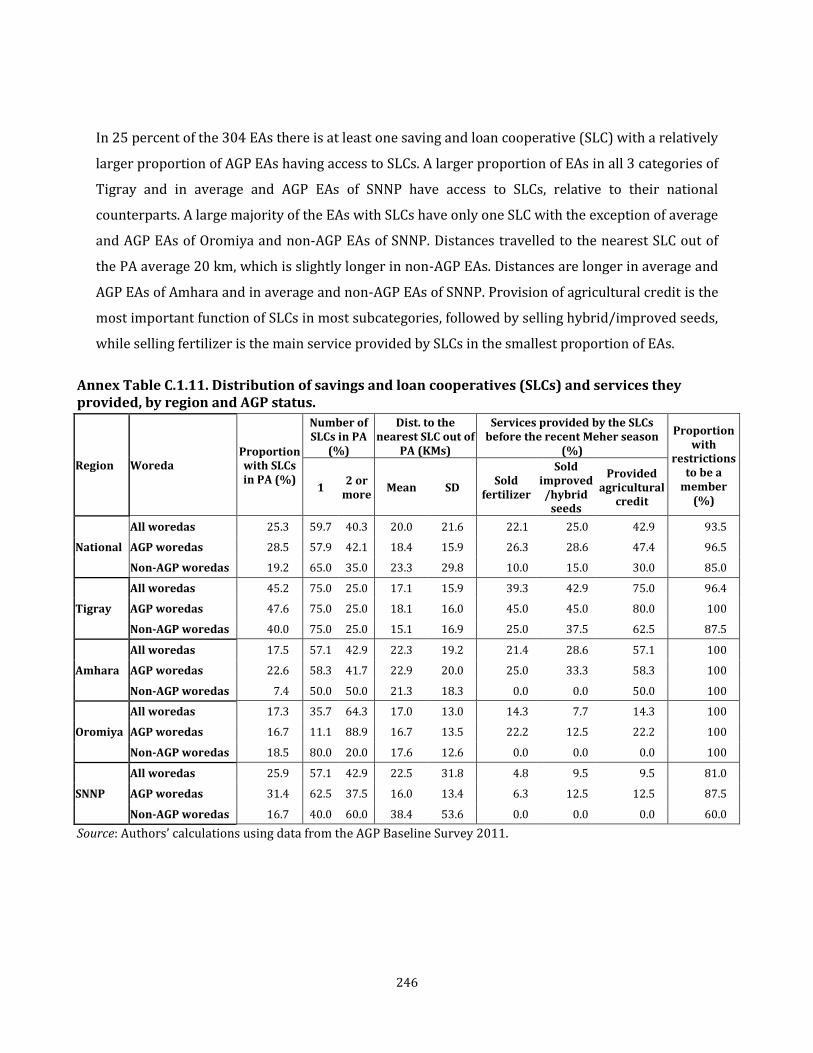
246
In 25 percent of the 304 EAs there is at least one saving and loan cooperative (SLC) with a relatively
larger proportion of AGP EAs having access to SLCs. A larger proportion of EAs in all 3 categories of
Tigray and in average and AGP EAs of SNNP have access to SLCs, relative to their national
counterparts. A large majority of the EAs with SLCs have only one SLC with the exception of average
and AGP EAs of Oromiya and non-AGP EAs of SNNP. Distances travelled to the nearest SLC out of
the PA average 20 km, which is slightly longer in non-AGP EAs. Distances are longer in average and
AGP EAs of Amhara and in average and non-AGP EAs of SNNP. Provision of agricultural credit is the
most important function of SLCs in most subcategories, followed by selling hybrid/improved seeds,
while selling fertilizer is the main service provided by SLCs in the smallest proportion of EAs.
Annex Table C.1.11. Distribution of savings and loan cooperatives (SLCs) and services they provided, by region and AGP status.
Region Woreda Proportion with SLCs in PA (%)
Number of SLCs in PA
(%)
Dist. to the nearest SLC out of
PA (KMs)
Services provided by the SLCs before the recent Meher season
(%)
Proportion with
restrictions to be a
member (%)
1 2 or
more Mean SD
Sold fertilizer
Sold improved
/hybrid seeds
Provided agricultural
credit
National
All woredas 25.3 59.7 40.3 20.0 21.6 22.1 25.0 42.9 93.5
AGP woredas 28.5 57.9 42.1 18.4 15.9 26.3 28.6 47.4 96.5
Non-AGP woredas 19.2 65.0 35.0 23.3 29.8 10.0 15.0 30.0 85.0
Tigray
All woredas 45.2 75.0 25.0 17.1 15.9 39.3 42.9 75.0 96.4
AGP woredas 47.6 75.0 25.0 18.1 16.0 45.0 45.0 80.0 100
Non-AGP woredas 40.0 75.0 25.0 15.1 16.9 25.0 37.5 62.5 87.5
Amhara
All woredas 17.5 57.1 42.9 22.3 19.2 21.4 28.6 57.1 100
AGP woredas 22.6 58.3 41.7 22.9 20.0 25.0 33.3 58.3 100
Non-AGP woredas 7.4 50.0 50.0 21.3 18.3 0.0 0.0 50.0 100
Oromiya
All woredas 17.3 35.7 64.3 17.0 13.0 14.3 7.7 14.3 100
AGP woredas 16.7 11.1 88.9 16.7 13.5 22.2 12.5 22.2 100
Non-AGP woredas 18.5 80.0 20.0 17.6 12.6 0.0 0.0 0.0 100
SNNP
All woredas 25.9 57.1 42.9 22.5 31.8 4.8 9.5 9.5 81.0
AGP woredas 31.4 62.5 37.5 16.0 13.4 6.3 12.5 12.5 87.5
Non-AGP woredas 16.7 40.0 60.0 38.4 53.6 0.0 0.0 0.0 60.0
Source: Authors’ calculations using data from the AGP Baseline Survey 2011.

247
Producer associations operate in 24.4 percent of the EAs with the proportion slightly larger in non-
AGP EAs. With the exception of non-AGP EAs of Amhara both Tigray and Amhara have relatively
larger proportion of EAs with producer associations. All 3 categories of EAs in Oromiya and SNNP
have smaller proportion of producer associations. In a large majority of the EAs there is a single
operational producer association. In the EAs where there are no producer associations the closest
outside the PA is about 19 km away, with a slightly longer distance in non-AGP EAs. About 64
percent of the producer associations sell fertilizers and 61 percent sell improved or hybrid seeds.
Technical assistance on crop production, assistance in crop marketing, and provision of credits are
the next three important functions of producer associations. This general pattern broadly holds in
the rest of the subsamples.
Annex Table C.1.12. Distribution of producers associations (PAs) and services they provided, by region and AGP status.
Region Woreda
Propor tion with
PAs in PA (%)
Number of PAs in PA (%) Dist. to
the nearest
PA (km)
Services provided by the PAs before the recent Meher season (%) Proportion
with restrictions to be a member
(%) 1
2 or more
Sold fertilizer
Sold improved/hybrid
seeds
Provided agricultural
credit
Provided technical advice on
crop production
Provided assistance
in marketing of crops
National
All woredas 24.4 82.9 17.1 18.7 63.5 60.8 37.8 54.1 45.9 94.6
AGP woredas 22.0 87.8 12.2 17.2 59.1 56.8 45.5 45.5 52.3 93.2
Non-AGP woredas 29.1 75.9 24.1 21.7 70.0 66.7 26.7 66.7 36.7 96.7
Tigray
All woredas 41.9 76.0 24.0 15.4 53.8 53.8 38.5 46.2 46.2 92.3
AGP woredas 33.3 76.9 23.1 14.6 35.7 28.6 21.4 28.6 50.0 85.7
Non-AGP woredas 60.0 75.0 25.0 17.2 75.0 83.3 58.3 66.7 41.7 100
Amhara
All woredas 32.5 95.8 4.2 21.4 84.6 84.6 53.8 57.7 57.7 100
AGP woredas 35.8 100.0 0.0 20.7 84.2 89.5 73.7 52.6 57.9 100
Non-AGP woredas 25.9 83.3 16.7 22.2 85.7 71.4 0.0 71.4 57.1 100
Oromiya
All woredas 16.0 75.0 25.0 17.0 53.8 53.8 23.1 61.5 30.8 92.3
AGP woredas 13.0 83.3 16.7 17.1 57.1 57.1 28.6 57.1 42.9 85.7
Non-AGP woredas 22.2 66.7 33.3 16.8 50.0 50.0 16.7 66.7 16.7 100
SNNP
All woredas 11.3 77.8 22.2 19.5 44.4 22.2 11.1 55.6 33.3 88.9
AGP woredas 7.8 75.0 25.0 15.9 25.0 0.0 25.0 50.0 50.0 100
Non-AGP woredas 17.2 80.0 20.0 30.9 60.0 40.0 0.0 60.0 20.0 80.0
Source: Authors’ calculations using data from the AGP Baseline Survey, 2011.

248
In only 6.3 percent of the 304 EAs do small money and financial institutions (MFIs) operate with a
slightly higher proportion in AGP EAs. Proportionately more MFIs operate in Tigray and SNNP and
the reverse is true in Amhara and Oromiya, particularly there are no MFIs in non-AGP EAs of
Oromiya. Nationally, more than one MFI operate in a large majority of the EAs. This is mainly
influenced by SNNP, in which all EAs have 2 or more MFIs.
Residents of the 285 EAs where there are no MFIs travel about 19 km to the nearest MFI outside
the PA. The distance ranges from 11.2 km for an average resident of SNNP to 16.5 km in Amhara.
Where available, MFIs mostly provide timely credit. Credit is provided by MFIs in about 59 percent
of the EAs surveyed. With the exception of SNNP in which MFIs provide credit in only a quarter of
the EAs a minimum of two-thirds of the MFIs provide credit in all others where they operated.
Annex Table C.1.13. Distribution of banks and small microfinance institutions (MFIs) and services provided by MFIs, by region and AGP status
Region Woreda Proportion with MFIs in PA (%)
Number of MFIs in PA (%)
Distance to the nearest MFI out of
PA (km)
Proportion in which MFIs provided credit
before the most recent Meher season
(%) 1
2 or more
Mean SD
National
All woredas 6.3 47.4 52.6 18.9 14.7 58.8
AGP woredas 6.5 46.2 53.8 18.8 14.6 61.5
Non-AGP woredas 5.8 50.0 50.0 19.0 14.9 50.0
Tigray
All woredas 11.3 71.4 28.6 17.5 12.6 71.4
AGP woredas 9.5 50.0 50.0 19.0 14.0 75.0
Non-AGP woredas 15.0 100.0 0.0 14.2 8.3 66.7
Amhara
All woredas 3.8 66.7 33.3 22.2 16.5 66.7
AGP woredas 3.8 100.0 0.0 22.4 18.1 100.0
Non-AGP woredas 3.7 0.0 100.0 21.8 13.6 0.0
Oromiya
All woredas 3.8 66.7 33.3 21.5 16.0 66.7
AGP woredas 5.7 66.7 33.3 19.0 13.2 66.7
Non-AGP woredas 0.0 _ _ 25.9 19.5 -
SNNP
All woredas 7.4 0.0 100.0 14.0 11.2 25.0
AGP woredas 7.8 0.0 100.0 15.0 11.7 25.0
Non-AGP woredas 6.7 0.0 100.0 12.2 10.2 -
Source: Authors’ calculations using data from the AGP Baseline Survey, 2011.

249