aggregation-based algebraic multigrid - [groupe...
TRANSCRIPT
Aggregation-based algebraic multigridfrom theory to fast solvers
Yvan Notay∗
Universite Libre de BruxellesService de Metrologie Nucleaire
CEMRACS, Marseille, July 18, 2012
∗ Supported by the Belgian FNRShttp://homepages.ulb.ac.be/∼ynotay
Aggregation-based algebraic multigrid – p.1
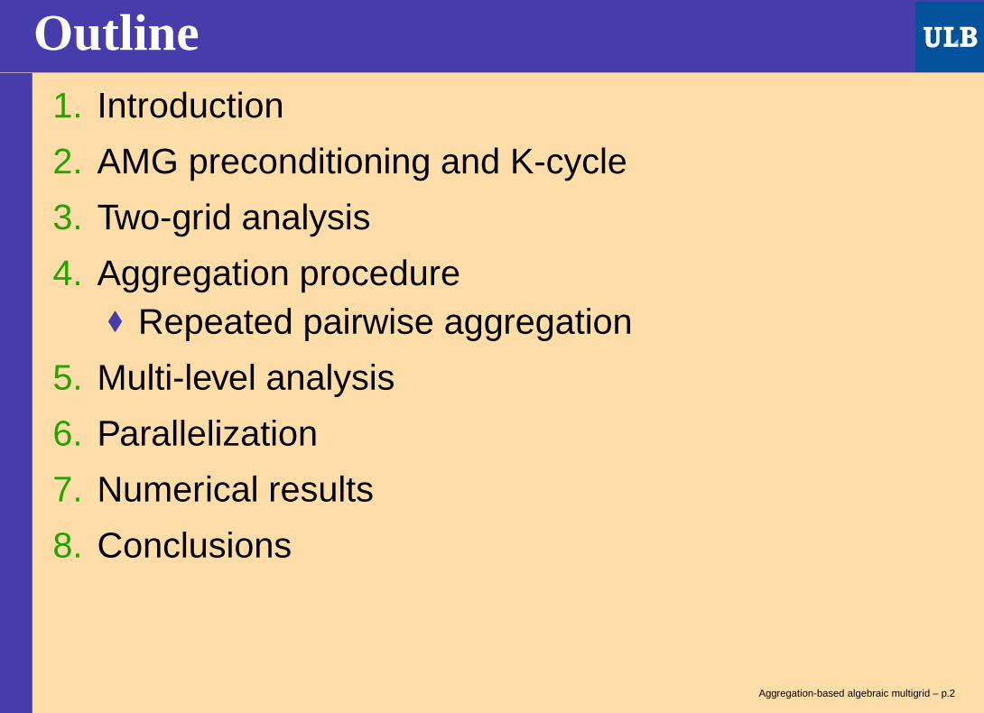
Outline1. Introduction
2. AMG preconditioning and K-cycle
3. Two-grid analysis
4. Aggregation procedure Repeated pairwise aggregation
5. Multi-level analysis
6. Parallelization
7. Numerical results
8. Conclusions
Aggregation-based algebraic multigrid – p.2
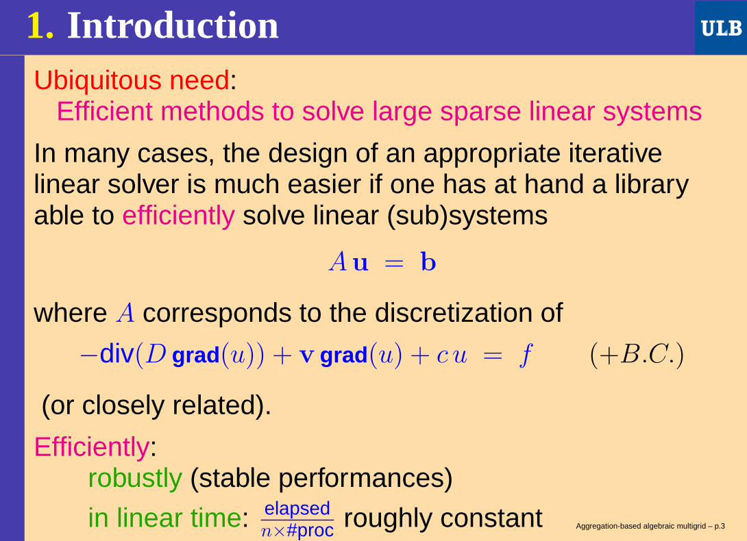
1. IntroductionUbiquitous need:
Efficient methods to solve large sparse linear systems
In many cases, the design of an appropriate iterativelinear solver is much easier if one has at hand a libraryable to efficiently solve linear (sub)systems
Au = b
where A corresponds to the discretization of
−div(D grad (u)) + v grad (u) + c u = f (+B.C.)
(or closely related).
Efficiently:robustly (stable performances)
in linear time: elapsedn×#proc roughly constant Aggregation-based algebraic multigrid – p.3

1. Introduction From Martin Gander talk:
Krylov subspace method needed for robustness
Aggregation-based algebraic multigrid – p.4

1. Introduction From Martin Gander talk:
Krylov subspace method needed for robustness From Ulrich Rüde talk:
multigrid needed for linear time
Aggregation-based algebraic multigrid – p.4

1. Introduction From Martin Gander talk:
Krylov subspace method needed for robustness From Ulrich Rüde talk:
multigrid needed for linear time Here: use multigrid as a preconditioner for Krylov
(combine multigrid with Krylov acceleration)
Aggregation-based algebraic multigrid – p.4

1. Introduction From Martin Gander talk:
Krylov subspace method needed for robustness From Ulrich Rüde talk:
multigrid needed for linear time Here: use multigrid as a preconditioner for Krylov
(combine multigrid with Krylov acceleration)
Why algebraic multigrid (AMG)? Geometric multigrid: needs a predefined set of grids AMG attempts to obtain the same effect using only the
information present in the system matrix A
(Reminder: effect = efficient damping of “smooth” errorcomponents, that can be seen only from large scale)
Aggregation-based algebraic multigrid – p.4

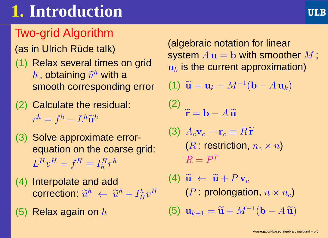
1. IntroductionTwo-grid Algorithm(as in Ulrich Rüde talk)(1) Relax several times on grid
h , obtaining uh with asmooth corresponding error
(2) Calculate the residual:rh = fh − Lh
uh
(3) Solve approximate error-equation on the coarse grid:LHvH = fH ≡ IH
hrh
(4) Interpolate and addcorrection: uh ← uh + Ih
HvH
(5) Relax again on h
Aggregation-based algebraic multigrid – p.5

1. IntroductionTwo-grid Algorithm(as in Ulrich Rüde talk)(1) Relax several times on grid
h , obtaining uh with asmooth corresponding error
(2) Calculate the residual:rh = fh − Lh
uh
(3) Solve approximate error-equation on the coarse grid:LHvH = fH ≡ IH
hrh
(4) Interpolate and addcorrection: uh ← uh + Ih
HvH
(5) Relax again on h
(algebraic notation for linearsystem Au = b with smoother M ;uk is the current approximation)
(1) u = uk +M−1(b− Auk)
(2)r = b−A u
(3) Acvc = rc ≡ R r
(R : restriction, nc × n)
(4) u ← u+ P vc
(P : prolongation, n× nc)
(5) uk+1 = u+M−1(b− A u)
Aggregation-based algebraic multigrid – p.5
1. IntroductionTwo-grid Algorithm(as in Ulrich Rüde talk)(1) Relax several times on grid
h , obtaining uh with asmooth corresponding error
(2) Calculate the residual:rh = fh − Lh
uh
(3) Solve approximate error-equation on the coarse grid:LHvH = fH ≡ IH
hrh
(4) Interpolate and addcorrection: uh ← uh + Ih
HvH
(5) Relax again on h
(algebraic notation for linearsystem Au = b with smoother M ;uk is the current approximation)
(1) u = uk +M−1(b− Auk)
(2)r = b−A u
(3) Acvc = rc ≡ R r
(R : restriction, nc × n)R = P T
(4) u ← u+ P vc
(P : prolongation, n× nc)
(5) uk+1 = u+M−1(b− A u)
Aggregation-based algebraic multigrid – p.5

1. IntroductionTwo-grid Algorithm(as in Ulrich Rüde talk)(1) Relax several times on grid
h , obtaining uh with asmooth corresponding error
(2) Calculate the residual:rh = fh − Lh
uh
(3) Solve approximate error-equation on the coarse grid:LHvH = fH ≡ IH
hrh
(4) Interpolate and addcorrection: uh ← uh + Ih
HvH
(5) Relax again on h
(algebraic notation for linearsystem Au = b with smoother M ;uk is the current approximation)
(1) u = uk +M−1(b− Auk)
(2)r = b−A u
(3) Acvc = rc ≡ R r
(R : restriction, nc × n)R = P T , Ac = RAP = P TAP
(4) u ← u+ P vc
(P : prolongation, n× nc)
(5) uk+1 = u+M−1(b− A u)
→ Try to obtain P from AAggregation-based algebraic multigrid – p.5

1. Intro: Why aggregation-basedAMG?Classical AMG Heuristic algorithms to mimic geometric multigrid
(Connectivity → set of coarse nodes;Matrix entries→ interpolation rules)
Need to be used recursively:Ac = P TAP→ Acc = P T
c Ac Pc , etcIs a good algorithm for A also good for Ac ?
Several variants and parameters;relevant choices depend on applications
Main difficulty:Find a good tradeoff between accuracy and themastering of “complexity” (i.e., the control of thesparsity in successive coarse grid matrices)
Aggregation-based algebraic multigrid – p.6

1. Intro: Aggregation-based AMGGroup nodes into aggregates Gi (partitioning of [1 , n])Each set corresponds to 1 coarse variable(and vice-versa)
G1
G2
G3
G4
Aggregation-based algebraic multigrid – p.7

1. Intro: Aggregation-based AMG
Prolongation P : Pij =
1 if i ∈ Gj
0 otherwiseExample
uc =
1
2
3
4
→
G1
G2
G3
G4
1
1
1
2
2
2
2
3
3 3
3
4
44
4
4
Aggregation-based algebraic multigrid – p.8

1. Intro: Aggregation-based AMGCoarse grid matrix: Ac = P T AP given by
(Ac)ij =∑
k∈Gi
∑
ℓ∈Gj
akℓ
G1
G2
G3
G4
→Tends to reproduce the stencil from the fine grid
Aggregation-based algebraic multigrid – p.9
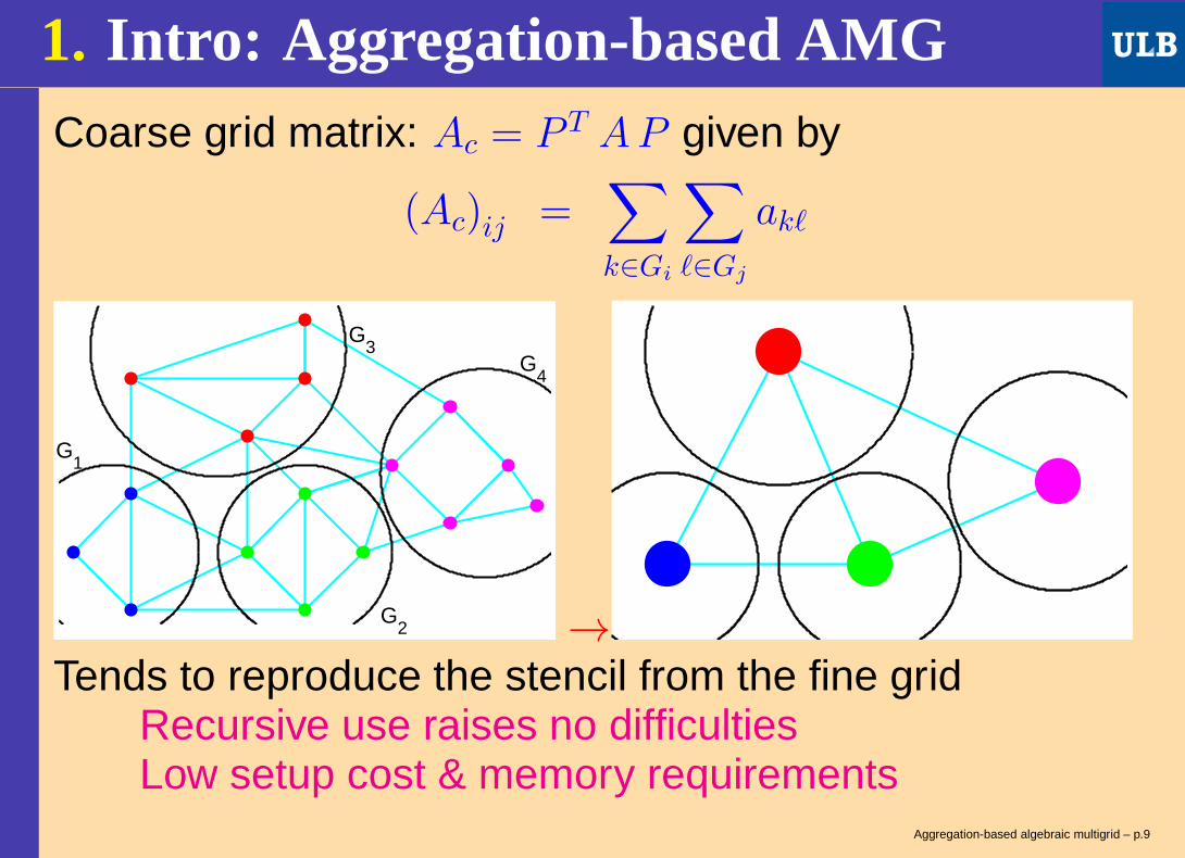
1. Intro: Aggregation-based AMGCoarse grid matrix: Ac = P T AP given by
(Ac)ij =∑
k∈Gi
∑
ℓ∈Gj
akℓ
G1
G2
G3
G4
→Tends to reproduce the stencil from the fine grid
Recursive use raises no difficultiesLow setup cost & memory requirements
Aggregation-based algebraic multigrid – p.9

1. Intro: Aggregation-based AMG Does not mimic any classical multigrid method Not efficient if the piecewise constant P just
substitutes the classical prolongation in a standardmultigrid scheme
→ has been overlooked for a long time
Aggregation-based algebraic multigrid – p.10

1. Intro: Aggregation-based AMG Does not mimic any classical multigrid method Not efficient if the piecewise constant P just
substitutes the classical prolongation in a standardmultigrid scheme
→ has been overlooked for a long time
Recent revival: Proper convergence theory (mimicry not
essential for a good interplay with the smoother) Efficient when combined with specific components:
preconditioner for a Krylov method, cheap smoother &K-cycle (Krylov for coarse problems – all levels)
Theory and efficient solver developed hand in handAggregation-based algebraic multigrid – p.10
Outline1. Introduction
2. AMG preconditioning and K-cycle
3. Two-grid analysis
4. Aggregation procedureRepeated pairwise aggregation
5. Multi-level analysis
6. Parallelization
7. Numerical results
8. Conclusions
Aggregation-based algebraic multigrid – p.11

2. AMG preconditioning and K-cycleReminder:Stationary iteration: uk+1 = uk +M−1(b− Auk)
Corresponding preconditioning step:vk = M−1
rk (rk = b− Auk)
Aggregation-based algebraic multigrid – p.12

2. AMG preconditioning and K-cycleReminder:Stationary iteration: uk+1 = uk +M−1(b− Auk)
Corresponding preconditioning step:vk = M−1
rk (rk = b− Auk)
→ for multigrid, rewrite the algorithm above as
uk+1 = uk + B(b− Auk) ;
B is the inverse of the preconditioner and
vk = B rk
the corresponding preconditioning step
Aggregation-based algebraic multigrid – p.12

2. AMG preconditioning and K-cycleBenefit of Krylov Relaxed convergence conditions Scaling-independent convergence,
characterized by the condition number (λi eig of BA) :
SPD: κ =maxi λi
mini λi=
λmax(BA)
λmin(BA)
General:maxi |λi|
miniℜe(λi)or
1
miniℜe(1/λi) miniℜe(λi)
(All eigs with positive real part) Accelerated convergence
Aggregation-based algebraic multigrid – p.13
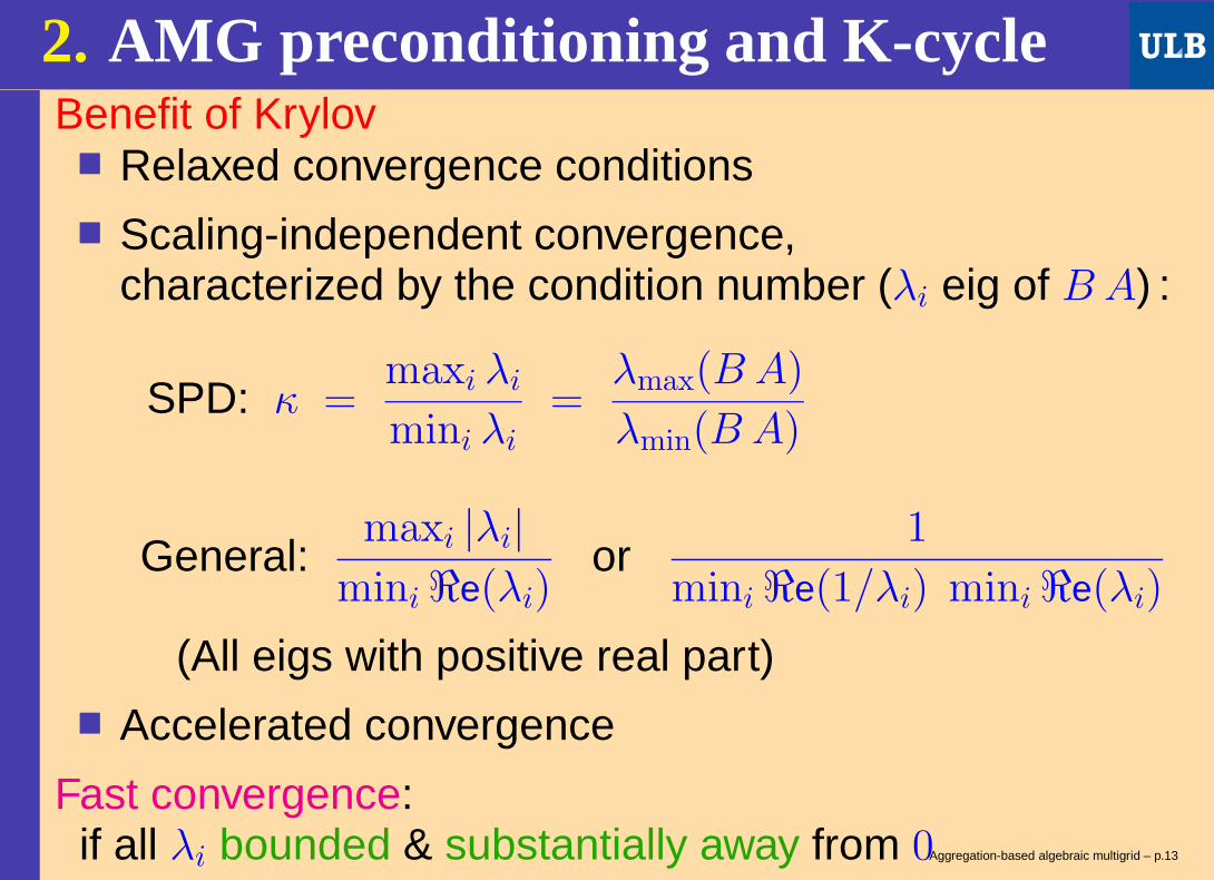
2. AMG preconditioning and K-cycleBenefit of Krylov Relaxed convergence conditions Scaling-independent convergence,
characterized by the condition number (λi eig of BA) :
SPD: κ =maxi λi
mini λi=
λmax(BA)
λmin(BA)
General:maxi |λi|
miniℜe(λi)or
1
miniℜe(1/λi) miniℜe(λi)
(All eigs with positive real part) Accelerated convergence
Fast convergence:if all λi bounded & substantially away from 0Aggregation-based algebraic multigrid – p.13

2. AMG preconditioning and K-cycleK-cycle Reminder: recursive use of the two-grid scheme:
Acvc = rc not solved exactly vc ← approximate solution from multigrid
step(s) to solve the coarse system 1 step → V-cycle
2 steps→W-cycle K-cycle: solve Acvc = rc with 2 steps of a Krylov
method with multigrid preconditioner at coarser level
(essentially: W-cycle with Krylov acceleration)
Aggregation-based algebraic multigrid – p.14
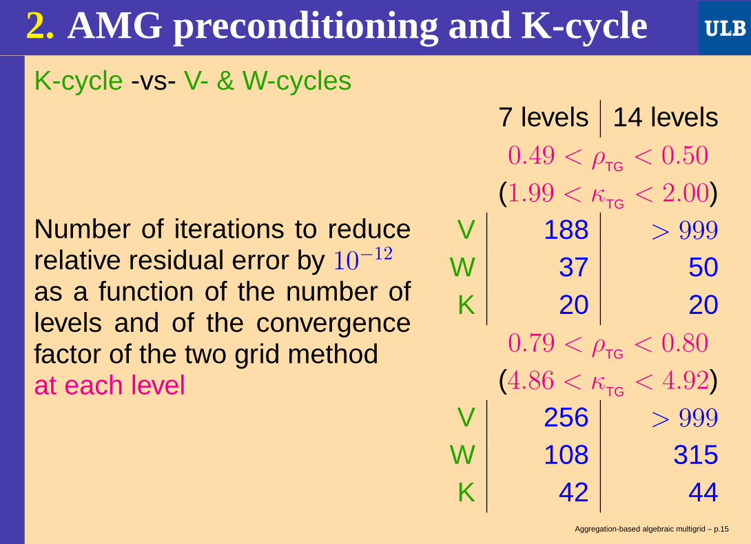
2. AMG preconditioning and K-cycleK-cycle -vs- V- & W-cycles
Number of iterations to reducerelative residual error by 10−12
as a function of the number oflevels and of the convergencefactor of the two grid methodat each level
7 levels 14 levels0.49 < ρTG < 0.50
(1.99 < κTG < 2.00)V 188 > 999
W 37 50K 20 20
0.79 < ρTG < 0.80
(4.86 < κTG < 4.92)V 256 > 999
W 108 315K 42 44
Aggregation-based algebraic multigrid – p.15

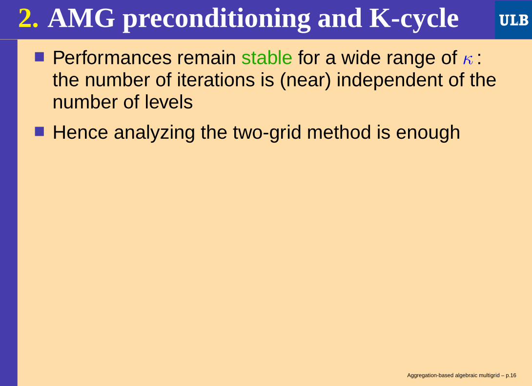
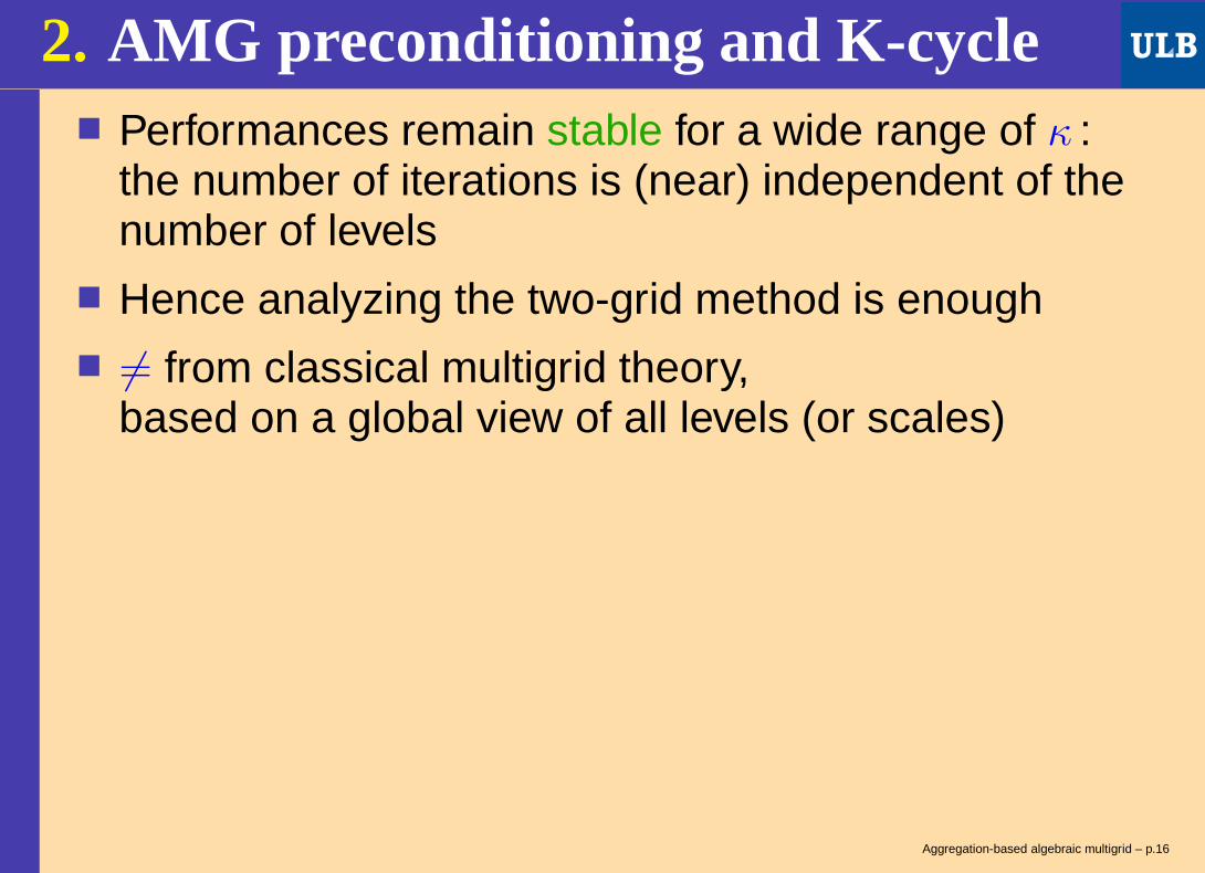
2. AMG preconditioning and K-cycle Performances remain stable for a wide range of κ :
the number of iterations is (near) independent of thenumber of levels
Aggregation-based algebraic multigrid – p.16
2. AMG preconditioning and K-cycle Performances remain stable for a wide range of κ :
the number of iterations is (near) independent of thenumber of levels
Hence analyzing the two-grid method is enough
Aggregation-based algebraic multigrid – p.16
2. AMG preconditioning and K-cycle Performances remain stable for a wide range of κ :
the number of iterations is (near) independent of thenumber of levels
Hence analyzing the two-grid method is enough 6= from classical multigrid theory,
based on a global view of all levels (or scales)
Aggregation-based algebraic multigrid – p.16

2. AMG preconditioning and K-cycle Performances remain stable for a wide range of κ :
the number of iterations is (near) independent of thenumber of levels
Hence analyzing the two-grid method is enough 6= from classical multigrid theory,
based on a global view of all levels (or scales) Classical multigrid: use “enough” smoothing steps to
have spectral radius as small as desired
Aggregation-based AMG:compensate for the larger condition number withKrylov, but also cheap smoothing stage(typically: one Gauss-Seidel sweep for pre- andpost-smoothing)
Aggregation-based algebraic multigrid – p.16

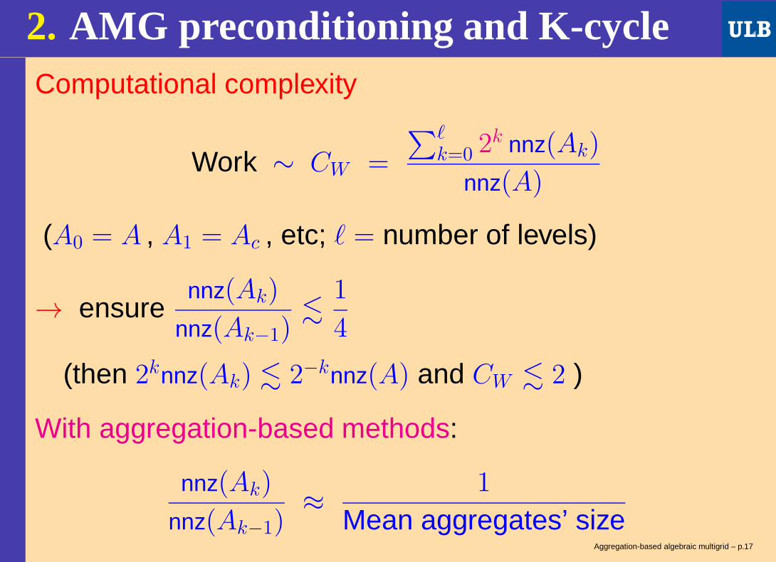
2. AMG preconditioning and K-cycleComputational complexity
Work ∼ CW =
∑ℓk=0 2
k nnz(Ak)
nnz(A)
(A0 = A , A1 = Ac , etc; ℓ = number of levels)
→ ensurennz(Ak)
nnz(Ak−1).
1
4
(then 2knnz(Ak) . 2−knnz(A) and CW . 2 )
Aggregation-based algebraic multigrid – p.17
2. AMG preconditioning and K-cycleComputational complexity
Work ∼ CW =
∑ℓk=0 2
k nnz(Ak)
nnz(A)
(A0 = A , A1 = Ac , etc; ℓ = number of levels)
→ ensurennz(Ak)
nnz(Ak−1).
1
4
(then 2knnz(Ak) . 2−knnz(A) and CW . 2 )
With aggregation-based methods:
nnz(Ak)
nnz(Ak−1)≈
1
Mean aggregates’ sizeAggregation-based algebraic multigrid – p.17
Outline1. Introduction
2. AMG preconditioning and K-cycle
3. Two-grid analysis
4. Aggregation procedureRepeated pairwise aggregation
5. Multi-level analysis
6. Parallelization
7. Numerical results
8. Conclusions
Aggregation-based algebraic multigrid – p.18

3. Two-grid analysisThe algebraic convergence theory: yields meaningful bounds
(actual convergence as proved often OK)
Aggregation-based algebraic multigrid – p.19

3. Two-grid analysisThe algebraic convergence theory: yields meaningful bounds
(actual convergence as proved often OK) is compatible with irregular geometries, unstructured
grids, jumps in coefficients, etc(guarantees essentially the same bound)
Aggregation-based algebraic multigrid – p.19

3. Two-grid analysisThe algebraic convergence theory: yields meaningful bounds
(actual convergence as proved often OK) is compatible with irregular geometries, unstructured
grids, jumps in coefficients, etc(guarantees essentially the same bound)
requires M-matrix, but has natural heuristic extensions
Aggregation-based algebraic multigrid – p.19

3. Two-grid analysisThe algebraic convergence theory: yields meaningful bounds
(actual convergence as proved often OK) is compatible with irregular geometries, unstructured
grids, jumps in coefficients, etc(guarantees essentially the same bound)
requires M-matrix, but has natural heuristic extensions whenever applicable, holds at every level of the
hierarchy
Aggregation-based algebraic multigrid – p.19
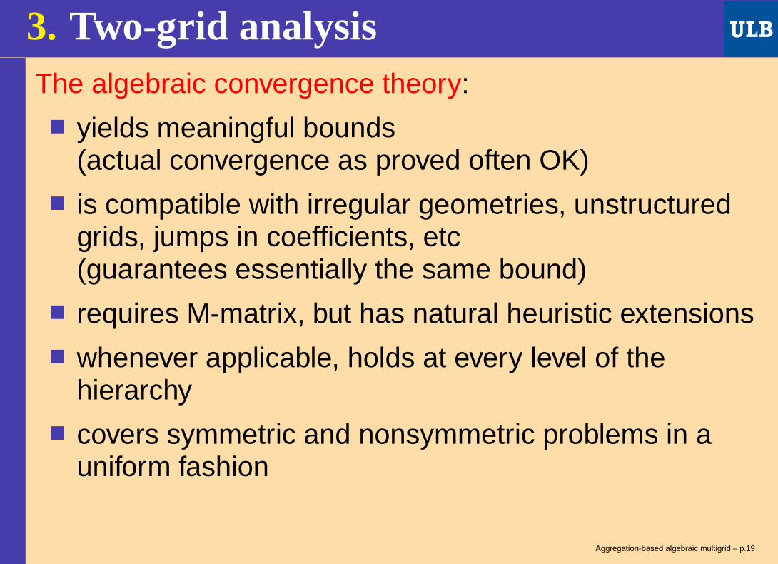
3. Two-grid analysisThe algebraic convergence theory: yields meaningful bounds
(actual convergence as proved often OK) is compatible with irregular geometries, unstructured
grids, jumps in coefficients, etc(guarantees essentially the same bound)
requires M-matrix, but has natural heuristic extensions whenever applicable, holds at every level of the
hierarchy covers symmetric and nonsymmetric problems in a
uniform fashion
The aggregation algorithm we use is entirely based on thetheory and its heuristic extensions Aggregation-based algebraic multigrid – p.19

3. Two-grid analysis Method used as a preconditioner for CG or GCR
→ Fast convergence if the eigenvalues λi of thepreconditioned matrix are:
bounded substantially away from 0
Using a standard smoother (e.g., Gauss-Seidel),the eigenvalues are bounded independently of P
If P = 0 the eigenvalues associated with “smooth”modes are in general very small → Main difficulty: λi substantially away from 0 Role of the coarse grid correction: move the small
eigenvalues enough to the right(Guideline for the choice of P ) Aggregation-based algebraic multigrid – p.20

3. Two-grid analysis: λi away from 0SPD caseMain identity [Falgout, Vassilevski & Zikatanov (2005)]:
λmin =1
κ(A , P )
with
κ(A,P ) = ω−1 supv 6=0
vTD
(I − P (P TDP )−1P TD
)v
vTAv
Aggregation-based algebraic multigrid – p.21

3. Two-grid analysis: λi away from 0SPD caseMain identity [Falgout, Vassilevski & Zikatanov (2005)]:
λmin =1
κ(A , P )
with
κ(A,P ) = ω−1 supv 6=0
vTD
(I − P (P TDP )−1P TD
)v
vTAv
General case [YN (2010)]For any λi :
ℜe(λi) ≥1
κ(AS , P )with AS = 1
2(A+ AT )
The analysis of the SPD case can be sufficientAggregation-based algebraic multigrid – p.21
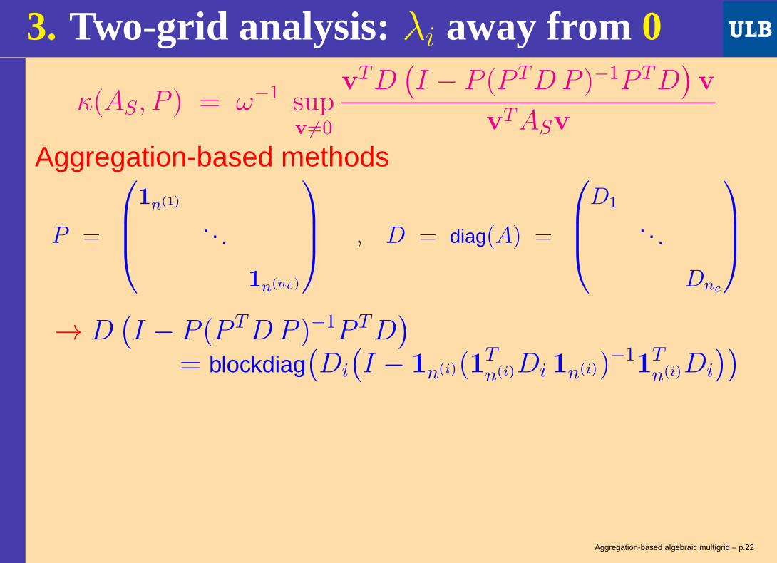
3. Two-grid analysis: λi away from 0
κ(AS, P ) = ω−1 supv 6=0
vTD
(I − P (P TDP )−1P TD
)v
vTASv
Aggregation-based methods
P =
1n(1)
. . .
1n(nc)
, D = diag(A) =
D1
. . .
Dnc
→ D(I − P (P TDP )−1P TD
)
= blockdiag(Di
(I − 1n(i)(1T
n(i)Di 1n(i))−11Tn(i)Di
))
Aggregation-based algebraic multigrid – p.22

3. Two-grid analysis: λi away from 0
κ(AS, P ) = ω−1 supv 6=0
vTD
(I − P (P TDP )−1P TD
)v
vTASv
Aggregation-based methods
P =
1n(1)
. . .
1n(nc)
, D = diag(A) =
D1
. . .
Dnc
→ D(I − P (P TDP )−1P TD
)
= blockdiag(Di
(I − 1n(i)(1T
n(i)Di 1n(i))−11Tn(i)Di
))
→ find Ab , Ar nonnegative definite s.t. AS = Ab +Ar with
Ab =
A(S)G1
. . .
AG
(S)nc
Aggregation-based algebraic multigrid – p.22

3. Two-grid analysis: λi away from 0
κ(AS, P ) ≤ ω−1 supv 6=0
vTD
(I − P (P TDP )−1P TD
)v
vTAbv
Aggregation-based methods
P =
1n(1)
. . .
1n(nc)
, D = diag(A) =
D1
. . .
Dnc
→ D(I − P (P TDP )−1P TD
)
= blockdiag(Di
(I − 1n(i)(1T
n(i)Di 1n(i))−11Tn(i)Di
))
→ find Ab , Ar nonnegative definite s.t. AS = Ab +Ar with
Ab =
A(S)G1
. . .
AG
(S)nc
Aggregation-based algebraic multigrid – p.22

3. Two-grid analysis: λi away from 0Aggregate Quality
µG = ω−1 supv/∈N (A
(S)G )
vTDG(I − 1G(1
TGDG1G)
−11TGDG)v
vTA(S)G v
,
Then: κ(AS , P ) ≤ maxi µGi
Controlling µGiensures that eigenvalues are away from 0
Aggregation-based algebraic multigrid – p.23

3. Two-grid analysis: λi away from 0Aggregate Quality
µG = ω−1 supv/∈N (A
(S)G )
vTDG(I − 1G(1
TGDG1G)
−11TGDG)v
vTA(S)G v
,
Then: κ(AS , P ) ≤ maxi µGi
Controlling µGiensures that eigenvalues are away from 0
A(S)G : Computed from AS = Ab + Ar with Ar1 = 0
Rigorous for M-matrices s.t. AS1 ≥ 0(then Ab , Ar guaranteed nonnegative definite)
Heuristic in other cases(Ar could have negative eigenvalue(s))
Aggregation-based algebraic multigrid – p.23

Outline1. Introduction
2. AMG preconditioning and K-cycle
3. Two-grid analysis
4. Aggregation procedureRepeated pairwise aggregation
5. Multi-level analysis
6. Parallelization
7. Numerical results
8. Conclusions
Aggregation-based algebraic multigrid – p.24
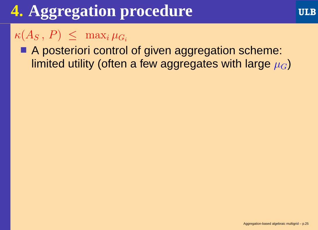
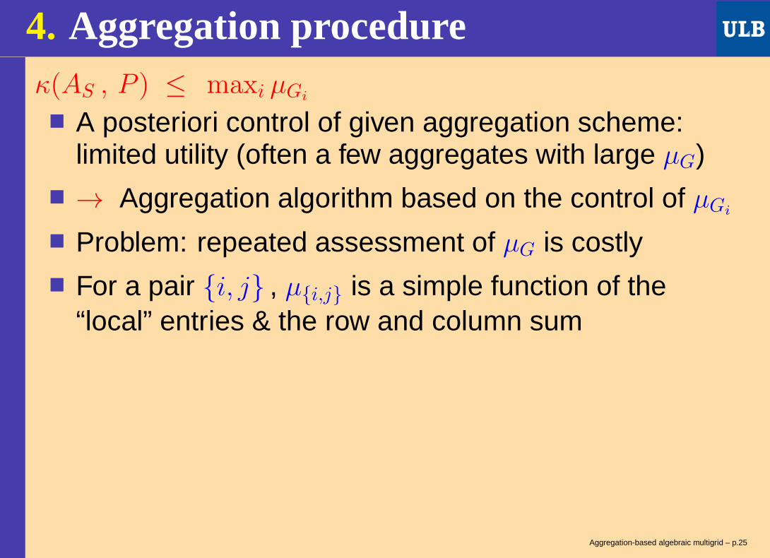
4. Aggregation procedureκ(AS , P ) ≤ maxi µGi
A posteriori control of given aggregation scheme:limited utility (often a few aggregates with large µG)
Aggregation-based algebraic multigrid – p.25

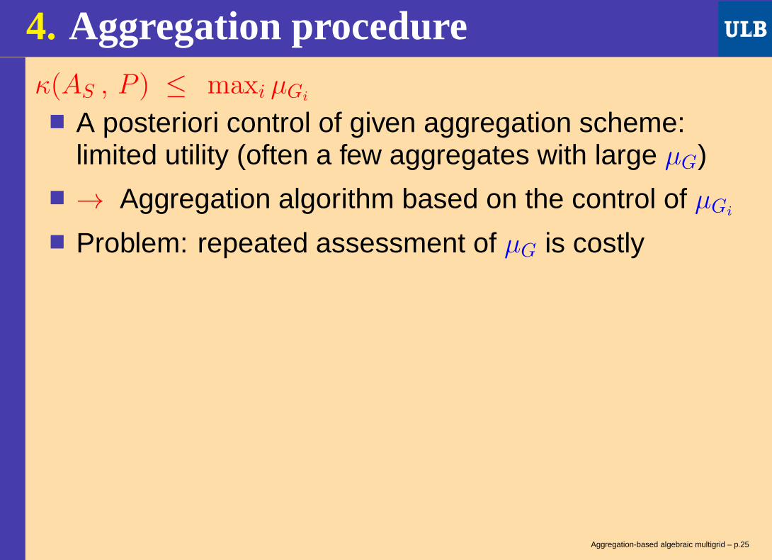
4. Aggregation procedureκ(AS , P ) ≤ maxi µGi
A posteriori control of given aggregation scheme:limited utility (often a few aggregates with large µG)
→ Aggregation algorithm based on the control of µGi
Aggregation-based algebraic multigrid – p.25
4. Aggregation procedureκ(AS , P ) ≤ maxi µGi
A posteriori control of given aggregation scheme:limited utility (often a few aggregates with large µG)
→ Aggregation algorithm based on the control of µGi
Problem: repeated assessment of µG is costly
Aggregation-based algebraic multigrid – p.25
4. Aggregation procedureκ(AS , P ) ≤ maxi µGi
A posteriori control of given aggregation scheme:limited utility (often a few aggregates with large µG)
→ Aggregation algorithm based on the control of µGi
Problem: repeated assessment of µG is costly For a pair i, j , µi,j is a simple function of the
“local” entries & the row and column sum
Aggregation-based algebraic multigrid – p.25

4. Aggregation procedureκ(AS , P ) ≤ maxi µGi
A posteriori control of given aggregation scheme:limited utility (often a few aggregates with large µG)
→ Aggregation algorithm based on the control of µGi
Problem: repeated assessment of µG is costly For a pair i, j , µi,j is a simple function of the
“local” entries & the row and column sum
µG = ω−1 supz/∈N (A
(S)G )
zT DG(I−1G
(1TGDG1G
)−1
1TGDG) z
zT A(S)G z
It is always cheap to check that µG < κTG holds:
ZG = κTG A(S)G − ω−1DG(I − 1G
(1TGDG1G
)−11TGDG)
is nonnegative definite if no negative pivot occurs whileperforming an LDLT factorization Aggregation-based algebraic multigrid – p.25

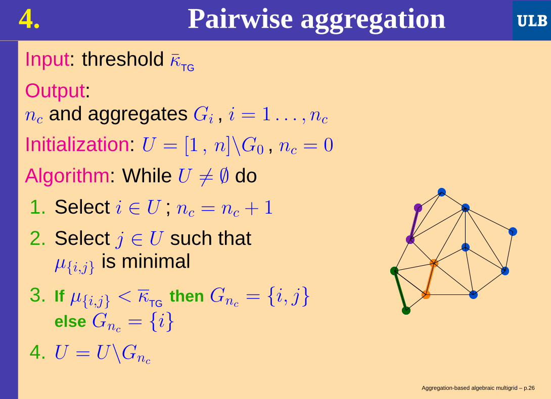
4. Pairwise aggregationInput: threshold κTG
Output:nc and aggregates Gi , i = 1 . . . , nc
Initialization: U = [1 , n]\G0 , nc = 0
Algorithm: While U 6= ∅ do
1. Select i ∈ U ; nc = nc + 1
2. Select j ∈ U such thatµi,j is minimal
3. If µi,j < κTG then Gnc= i, j
else Gnc= i
4. U = U\Gnc
Aggregation-based algebraic multigrid – p.26

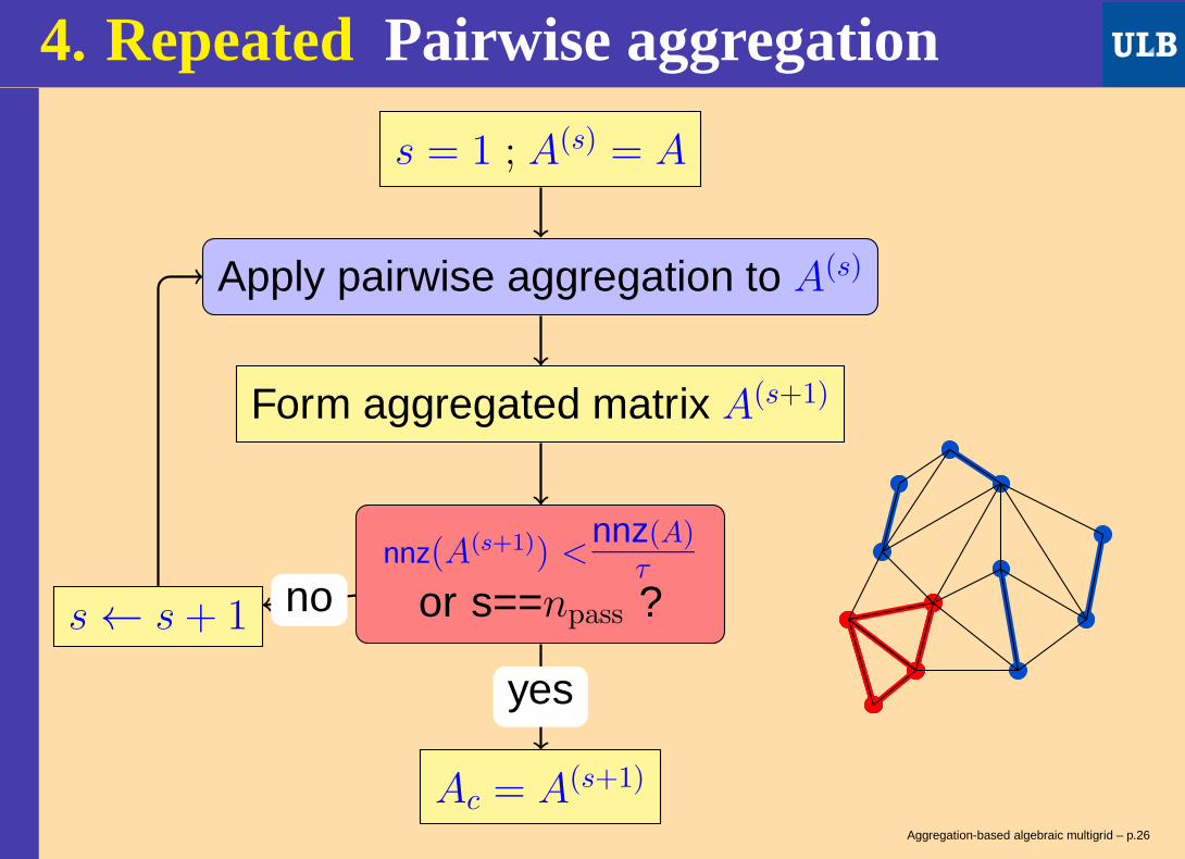
4. RepeatedPairwise aggregation
s = 1 ; A(s) = A
nnz(A(s+1)) <nnz(A)
τ
or s==npass ?
Apply pairwise aggregation to A(s)
Form aggregated matrix A(s+1)
s← s+ 1
Ac = A(s+1)
no
yes
Aggregation-based algebraic multigrid – p.26
4. RepeatedPairwise aggregation
s = 1 ; A(s) = A
nnz(A(s+1)) <nnz(A)
τ
or s==npass ?
Apply pairwise aggregation to A(s)
Form aggregated matrix A(s+1)
s← s+ 1
Ac = A(s+1)
no
yes
Aggregation-based algebraic multigrid – p.26

4. RepeatedPairwise aggregation
s = 1 ; A(s) = A
nnz(A(s+1)) <nnz(A)
τ
or s==npass ?
Apply pairwise aggregation to A(s)
Form aggregated matrix A(s+1)
s← s+ 1
Ac = A(s+1)
no
yes
Aggregation-based algebraic multigrid – p.26

4. RepeatedPairwise aggregation
s = 1 ; A(s) = A
nnz(A(s+1)) <nnz(A)
τ
or s==npass ?
Apply pairwise aggregation to A(s)
Form aggregated matrix A(s+1)
s← s+ 1
Ac = A(s+1)
Check µG < κTG in A
no
yes
Aggregation-based algebraic multigrid – p.26

4. RepeatedPairwise aggregation
s = 1 ; A(s) = A
nnz(A(s+1)) <nnz(A)
τ
or s==npass ?
Apply pairwise aggregation to A(s)
Form aggregated matrix A(s+1)
s← s+ 1
Ac = A(s+1)
Check µG < κTG in A
no
yes
Aggregation-based algebraic multigrid – p.26
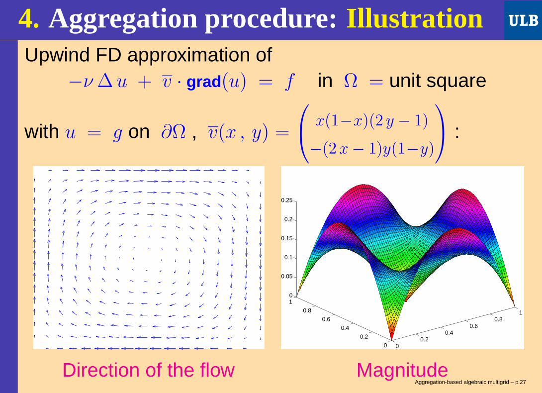
4. Aggregation procedure: IllustrationUpwind FD approximation of
−ν∆u + v · grad (u) = f in Ω = unit square
with u = g on ∂Ω , v(x , y) =
x(1−x)(2 y − 1)
−(2x− 1)y(1−y)
:
00.2
0.40.6
0.81
0
0.2
0.4
0.6
0.8
10
0.05
0.1
0.15
0.2
0.25
Direction of the flow MagnitudeAggregation-based algebraic multigrid – p.27

4. Aggregation procedure: Illustrationν = 1 : diffusion dominating (near symmetric)
Aggregation Spectrum
0 0.2 0.4 0.6 0.8 1
−0.5
0
0.5
+ : σ(I − T ) — : theory¨¨ : σ(ωD−1A) (convex hull)
Aggregation-based algebraic multigrid – p.28
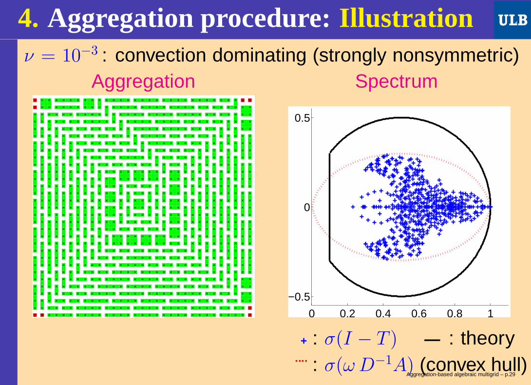
4. Aggregation procedure: Illustrationν = 10−3 : convection dominating (strongly nonsymmetric)
Aggregation Spectrum
0 0.2 0.4 0.6 0.8 1
−0.5
0
0.5
+ : σ(I − T ) — : theory¨¨ : σ(ωD−1A) (convex hull)
Aggregation-based algebraic multigrid – p.29

Outline1. Introduction
2. AMG preconditioning and K-cycle
3. Two-grid analysis
4. Aggregation procedureRepeated pairwise aggregation
5. Multi-level analysis
6. Parallelization
7. Numerical results
8. Conclusions
Aggregation-based algebraic multigrid – p.30

5. Multi -level analysisRequires to exchange the K-cycle (Krylov acceleration)for the AMLI-cycle (polynomial acceleration; i.e., frozencoefficients) less flexible: requires a known bound ρ on the two-grid
convergence factor less efficient in practice avoid nonlinearities→ convergence proof easier upper bound on the convergence rate independent of
the number of levels can be guaranteed with the soleassumption that ρ is below a given threshold
Aggregation-based algebraic multigrid – p.31

5. Multi -level analysisRequires to exchange the K-cycle (Krylov acceleration)for the AMLI-cycle (polynomial acceleration; i.e., frozencoefficients) less flexible: requires a known bound ρ on the two-grid
convergence factor less efficient in practice avoid nonlinearities→ convergence proof easier upper bound on the convergence rate independent of
the number of levels can be guaranteed with the soleassumption that ρ is below a given threshold
Our aggregation procedure: allows to choose ρ(for symmetric M-matrices with nonnegative row sum)
Aggregation-based algebraic multigrid – p.31

5. Multi -level analysis:final result The method is purely algebraic and applies to any
symmetric M-matrix with nonnegative row-sum
Aggregation-based algebraic multigrid – p.32

5. Multi -level analysis:final result The method is purely algebraic and applies to any
symmetric M-matrix with nonnegative row-sum The condition number is bounded
Aggregation-based algebraic multigrid – p.32

5. Multi -level analysis:final result The method is purely algebraic and applies to any
symmetric M-matrix with nonnegative row-sum The condition number is bounded
independently of mesh or problem size
Aggregation-based algebraic multigrid – p.32

5. Multi -level analysis:final result The method is purely algebraic and applies to any
symmetric M-matrix with nonnegative row-sum The condition number is bounded
independently of mesh or problem size independently of the number of levels
Aggregation-based algebraic multigrid – p.32
5. Multi -level analysis:final result The method is purely algebraic and applies to any
symmetric M-matrix with nonnegative row-sum The condition number is bounded
independently of mesh or problem size independently of the number of levels independently of matrix coefficients
(jumps, anisotropy, etc)
Aggregation-based algebraic multigrid – p.32

5. Multi -level analysis:final result The method is purely algebraic and applies to any
symmetric M-matrix with nonnegative row-sum The condition number is bounded
independently of mesh or problem size independently of the number of levels independently of matrix coefficients
(jumps, anisotropy, etc) independently of the regularity of the grid
Aggregation-based algebraic multigrid – p.32

5. Multi -level analysis:final result The method is purely algebraic and applies to any
symmetric M-matrix with nonnegative row-sum The condition number is bounded
independently of mesh or problem size independently of the number of levels independently of matrix coefficients
(jumps, anisotropy, etc) independently of the regularity of the grid independently of the type of refinement
(quasi uniformity, etc)
Aggregation-based algebraic multigrid – p.32

5. Multi -level analysis:final result The method is purely algebraic and applies to any
symmetric M-matrix with nonnegative row-sum The condition number is bounded
independently of mesh or problem size independently of the number of levels independently of matrix coefficients
(jumps, anisotropy, etc) independently of the regularity of the grid independently of the type of refinement
(quasi uniformity, etc) independently of any regularity assumption
Aggregation-based algebraic multigrid – p.32

5. Multi -level analysis:final resultWhy ?
Aggregation-based algebraic multigrid – p.33

5. Multi -level analysis:final resultWhy ?
. . . because the upper bound is 27.056
Aggregation-based algebraic multigrid – p.33
5. Multi -level analysis:final resultWhy ?
. . . because the upper bound is 27.056
Optimality requires in addition bounded complexity: can be proved for model problems on regular grids; no proof in general, but, in practice, no more
complexity issues than with other AMG schemes:coarsening parameters selected for this.
Aggregation-based algebraic multigrid – p.33

Outline1. Introduction
2. AMG preconditioning and K-cycle
3. Two-grid analysis
4. Aggregation procedureRepeated pairwise aggregation
5. Multi-level analysis
6. Parallelization
7. Numerical results
8. Conclusions
Aggregation-based algebraic multigrid – p.34

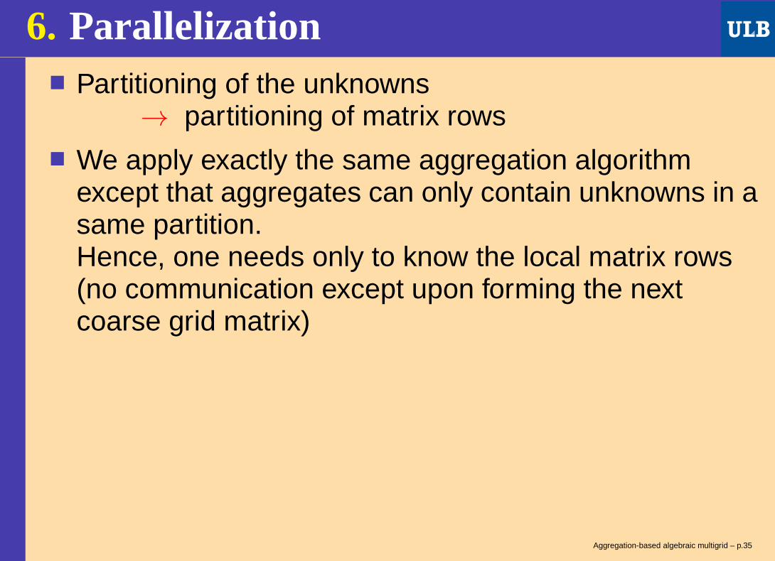
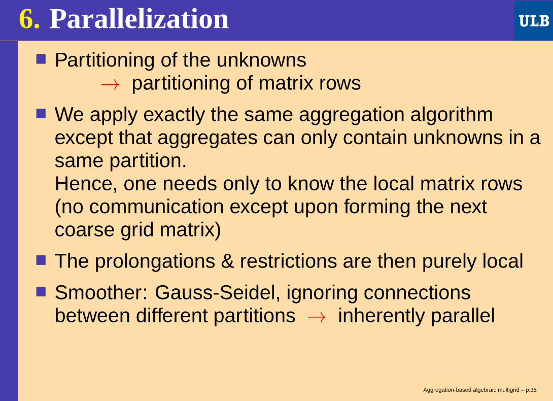
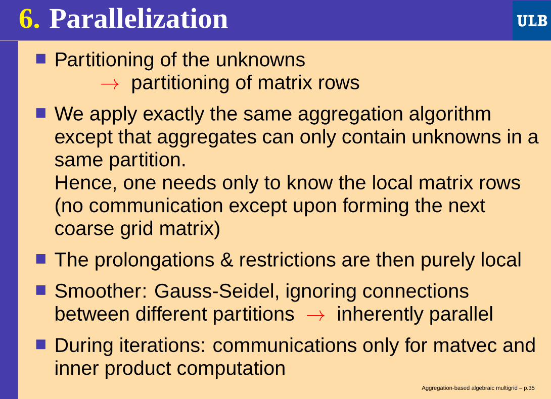
6. Parallelization Partitioning of the unknowns
→ partitioning of matrix rows
Aggregation-based algebraic multigrid – p.35
6. Parallelization Partitioning of the unknowns
→ partitioning of matrix rows We apply exactly the same aggregation algorithm
except that aggregates can only contain unknowns in asame partition.Hence, one needs only to know the local matrix rows(no communication except upon forming the nextcoarse grid matrix)
Aggregation-based algebraic multigrid – p.35

6. Parallelization Partitioning of the unknowns
→ partitioning of matrix rows We apply exactly the same aggregation algorithm
except that aggregates can only contain unknowns in asame partition.Hence, one needs only to know the local matrix rows(no communication except upon forming the nextcoarse grid matrix)
The prolongations & restrictions are then purely local
Aggregation-based algebraic multigrid – p.35
6. Parallelization Partitioning of the unknowns
→ partitioning of matrix rows We apply exactly the same aggregation algorithm
except that aggregates can only contain unknowns in asame partition.Hence, one needs only to know the local matrix rows(no communication except upon forming the nextcoarse grid matrix)
The prolongations & restrictions are then purely local Smoother: Gauss-Seidel, ignoring connections
between different partitions → inherently parallel
Aggregation-based algebraic multigrid – p.35
6. Parallelization Partitioning of the unknowns
→ partitioning of matrix rows We apply exactly the same aggregation algorithm
except that aggregates can only contain unknowns in asame partition.Hence, one needs only to know the local matrix rows(no communication except upon forming the nextcoarse grid matrix)
The prolongations & restrictions are then purely local Smoother: Gauss-Seidel, ignoring connections
between different partitions → inherently parallel During iterations: communications only for matvec and
inner product computationAggregation-based algebraic multigrid – p.35

Outline1. Introduction
2. AMG preconditioning and K-cycle
3. Two-grid analysis
4. Aggregation procedureRepeated pairwise aggregation
5. Multi-level analysis
6. Parallelization
7. Numerical results
8. Conclusions
Aggregation-based algebraic multigrid – p.36
7. Numerical resultsClassical AMG talk on application Description of the application (beautiful pictures) Description of the AMG strategy and needed tuning Numerical results, often not fully informative:
no robustness study on a comprehensive test suite; no comparison with state of the art competitors.
Aggregation-based algebraic multigrid – p.37

7. Numerical resultsThis talk Most applications ran by people downloading the code.
Some of those I am aware of: CFD, electrocardiology(in general, I don’t have the beautiful pictures at hand).
Aggregation-based algebraic multigrid – p.38
7. Numerical resultsThis talk Most applications ran by people downloading the code.
Some of those I am aware of: CFD, electrocardiology(in general, I don’t have the beautiful pictures at hand).
The code is used black box(adaptation neither sought nor needed)
I think the most important is the robustness on acomprehensive test suite
Aggregation-based algebraic multigrid – p.38

7. Numerical resultsThis talk Most applications ran by people downloading the code.
Some of those I am aware of: CFD, electrocardiology(in general, I don’t have the beautiful pictures at hand).
The code is used black box(adaptation neither sought nor needed)
I think the most important is the robustness on acomprehensive test suite
I like comparison with state of the art competitors
Aggregation-based algebraic multigrid – p.38

7. Numerical results Iterations stopped when ‖rk‖‖r0‖ < 10−6
Times reported are total elapsed times in seconds(including set up) per 106 unknowns
Test suite: discrete scalar elliptic PDEs SPD problems with jumps and all kind of anisotropy
in the coefficients (some with reentering corner) convection-diffusion problems with viscosity from1 → 10−6 and highly varying recirculating flow
FD on regular grids; 3 sizes:2D: h−1 = 600 , 1600 , 50003D: h−1 = 80 , 160 , 320
FE on (un)structured meshes (with different levels oflocal refinement); 2 sizes: n = 0.15e6 → n = 7.1e6
Aggregation-based algebraic multigrid – p.39
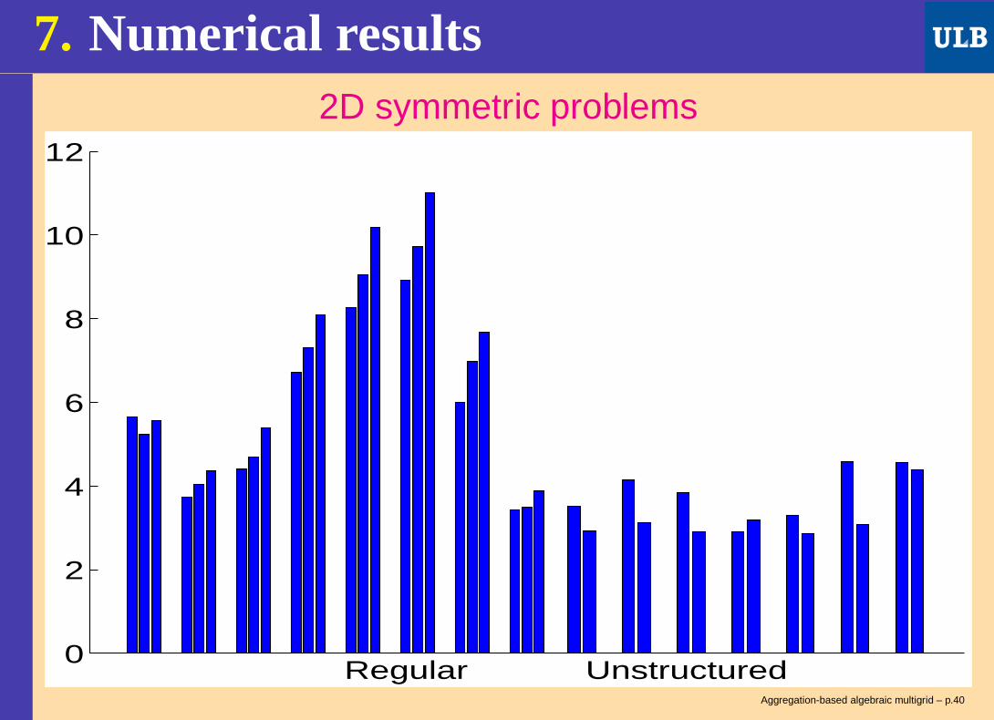
7. Numerical results2D symmetric problems
0
2
4
6
8
10
12
Regular UnstructuredAggregation-based algebraic multigrid – p.40

7. Numerical results3D symmetric problems
0
2
4
6
8
10
12
Regular UnstructuredAggregation-based algebraic multigrid – p.41

7. Numerical results2D nonsymmetric problems
0 5 10 15 20 25 300
2
4
6
8
10
12
Aggregation-based algebraic multigrid – p.42

7. Numerical results3D nonsymmetric problems
0 5 10 15 20 25 300
2
4
6
8
10
12
Aggregation-based algebraic multigrid – p.43

7. Numerical resultsComparison with other methods AMG(Hyp): classical AMG method as implemented in
the Hypre library (Boomer AMG) AMG(HSL): the classical AMG method as
implemented in the HSL library ILUPACK: efficient threshold-based ILU preconditioner Matlab \: Matlab sparse direct solver (UMFPACK)
All methods but the last with Krylov subspace acceleration
Aggregation-based algebraic multigrid – p.44

7. Numerical results
POISSON 2D, FD LAPLACE 2D, FE(P3)
104
105
106
107
108
3
5
10
20
50
100
200
400
AGMGAMG(Hyp)AMG(HSL)ILUPACKMatlab \
104
105
106
107
108
3
5
10
20
50
100
200
400
AGMGAMG(Hyp)AMG(HSL)ILUPACKMatlab \
33% of nonzero offdiag > 0
Aggregation-based algebraic multigrid – p.45

7. Numerical results
Poisson 2D, L-shaped, FE Convection-Diffusion 2D, FDUnstructured, Local refin. ν = 10−6
105
106
107
3
5
10
20
50
100
200
400
AGMGAMG(Hyp)AMG(HSL): coarsening failure in all casesILUPACKMatlab \
104
105
106
107
108
3
5
10
20
50
100
200
400
AGMGAMG(Hyp)AMG(HSL)ILUPACKMatlab \
Aggregation-based algebraic multigrid – p.46

7. Numerical results
POISSON 3D, FD LAPLACE 3D, FE(P3)
104
105
106
107
108
3
5
10
20
50
100
200
400
AGMGAMG(Hyp)AMG(HSL)ILUPACKMatlab \
104
105
106
107
3
5
10
20
50
100
200
400
AGMGAMG(Hyp)AMG(HSL)ILUPACKMatlab \
51% of nonzero offdiag > 0
Aggregation-based algebraic multigrid – p.47

7. Numerical results
Poisson 3D, FE Convection-Diffusion 3D, FDUnstructured, Local refin. ν = 10−6
104
105
106
107
3
5
10
20
50
100
200
400
AGMGAMG(Hyp)AMG(HSL)ILUPACKMatlab \
104
105
106
107
108
3
5
10
20
50
100
200
400
AGMGAMG(Hyp)AMG(HSL)ILUPACKMatlab \
Aggregation-based algebraic multigrid – p.48
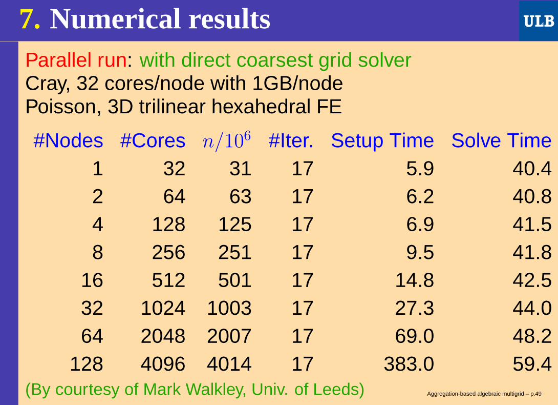
7. Numerical resultsParallel run: with direct coarsest grid solverCray, 32 cores/node with 1GB/nodePoisson, 3D trilinear hexahedral FE
#Nodes #Cores n/106 #Iter. Setup Time Solve Time1 32 31 17 5.9 40.42 64 63 17 6.2 40.84 128 125 17 6.9 41.58 256 251 17 9.5 41.8
16 512 501 17 14.8 42.532 1024 1003 17 27.3 44.064 2048 2007 17 69.0 48.2
128 4096 4014 17 383.0 59.4(By courtesy of Mark Walkley, Univ. of Leeds) Aggregation-based algebraic multigrid – p.49

7. Numerical resultsParallel run: with (new) iterative coarsest grid solverIntel(R) Xeon(R) CPU E5649 @ 2.53GHz3D problem with jumps, FD
#Nodes #Cores n/106 #Iter. Setup Time Solve Time1 8 64 12 14.9 89.
16 128 1026 16 17.4 191.48 384 3065 14 18.0 165.96 768 6155 13 17.4 170.
Aggregation-based algebraic multigrid – p.50

8. Conclusions Robust method for scalar elliptic PDEs
Aggregation-based algebraic multigrid – p.51

8. Conclusions Robust method for scalar elliptic PDEs Purely algebraic convergence theory:
do not depend on FE spaces, regularity assumption;applies also to the nonsymmetric case.
Aggregation-based algebraic multigrid – p.51

8. Conclusions Robust method for scalar elliptic PDEs Purely algebraic convergence theory:
do not depend on FE spaces, regularity assumption;applies also to the nonsymmetric case.
Can be used (and is used!) black box(does not require tuning or adaptation)
Faster than some solvers based on classical AMG
Aggregation-based algebraic multigrid – p.51
8. Conclusions Robust method for scalar elliptic PDEs Purely algebraic convergence theory:
do not depend on FE spaces, regularity assumption;applies also to the nonsymmetric case.
Can be used (and is used!) black box(does not require tuning or adaptation)
Faster than some solvers based on classical AMG Fairly small setup time: especially well suited when
only a modest accuracy is needed(e.g., linear solve within Newton steps)
Efficient parallelization
Aggregation-based algebraic multigrid – p.51

8. Conclusions Robust method for scalar elliptic PDEs Purely algebraic convergence theory:
do not depend on FE spaces, regularity assumption;applies also to the nonsymmetric case.
Can be used (and is used!) black box(does not require tuning or adaptation)
Faster than some solvers based on classical AMG Fairly small setup time: especially well suited when
only a modest accuracy is needed(e.g., linear solve within Newton steps)
Efficient parallelization Professional code available, free academic license
Aggregation-based algebraic multigrid – p.51

References Analysis of aggregation–based multigrid (with A. C. Muresan), SISC (2008).
Recursive Krylov-based multigrid cycles (with P. S. Vassilevski), NLAA (2008).
An aggregation-based algebraic multigrid method, ETNA (2010).
Algebraic analysis of two-grid methods: the nonsymmetric case, NLAA (2010).
Algebraic analysis of aggregation-based multigrid,(with A. Napov) NLAA (2011).
An algebraic multigrid method with guaranteed convergence rate(with A. Napov), SISC (2012).
Aggregation-based algebraic multigrid for convection-diffusion equations,SISC (2012, to appear).
AGMG software: Google AGMG(http://homepages.ulb.ac.be/~ynotay/AGMG)
Thank you for your attention !Aggregation-based algebraic multigrid – p.52