Research Division Federal Reserve Bank of St. Louis Working Paper Series

Aggregate Shocks and Labor Market Fluctuations

Helge Braun Reinout De Bock

and Riccardo DiCecio

Working Paper 2006-004A http://research.stlouisfed.org/wp/2006/2006-004.pdf

January 2006

FEDERAL RESERVE BANK OF ST. LOUIS Research Division

P.O. Box 442 St. Louis, MO 63166

______________________________________________________________________________________

The views expressed are those of the individual authors and do not necessarily reflect official positions of the Federal Reserve Bank of St. Louis, the Federal Reserve System, or the Board of Governors.

Federal Reserve Bank of St. Louis Working Papers are preliminary materials circulated to stimulate discussion and critical comment. References in publications to Federal Reserve Bank of St. Louis Working Papers (other than an acknowledgment that the writer has had access to unpublished material) should be cleared with the author or authors.

Aggregate Shocks and Labor Market Fluctuations�

Helge BraunNorthwestern University

Reinout De BockNorthwestern University

Riccardo DiCecioFederal Reserve Bank of St. Louis

January 2006

Abstract

This paper evaluates the dynamic response of worker �ows, job �ows, andvacancies to aggregate shocks in a structural vector autoregression. We iden-tify demand, monetary, and technology shocks by imposing sign restrictions onthe responses of output, in�ation, the interest rate, and the relative price ofinvestment. No restrictions are placed on the responses of job and worker �owsvariables. We �nd that both investment-speci�c and neutral technology shocksgenerate responses to job and worker �ows variables that are qualitatively sim-ilar to those induced by monetary and demand shocks. However, technologyshocks have more persistent e¤ects. The job �nding rate largely drives the re-sponse of unemployment, though the separation rate explains up to one third.For job �ows, the destruction margin is more important than the creation mar-gin in driving employment growth. Measuring reallocation from job �ows, we�nd that monetary and demand shocks do not have signi�cant e¤ects on cu-mulative job reallocation, whereas expansionary technology shocks have mildlynegative e¤ects. We also estimate shock-speci�c matching functions. Allowingfor a break in 1984:Q1 shows considerable subsample di¤erences in matchingelasticities and relative shock-speci�c e¢ ciency.JEL: C32, E24, E32, J63.Keywords: business cycles, job �ows, unemployment, vacancies, vector au-

toregressions, worker �ows.

�We are grateful to Larry Christiano, Martin Eichenbaum, Luca Dedola, Daniel Levy, ÉvaNagypál, Dale Mortensen, Frank Smets and seminar participants at the ECB for helpful comments.We thank Olivier Blanchard, Hoyt Bleakley, Steven Davis, Jonas Fisher, and Robert Shimer forsharing their data. Helge Braun and Reinout De Bock thank the research department at the St.Louis Fed and the ECB, respectively, for their hospitality. Reinout gratefully acknowledges �nan-cial support of a Dehousse Fellowship of the Speciaal Fonds voor Onderzoek at the University ofAntwerp. Any views expressed are our own and do not necessarily re�ect the views of the FederalReserve Bank of St. Louis or the Federal Reserve System. All errors are our own. Correspondingauthor: Riccardo DiCecio, Riccardo.DiCecio@stls.frb.org

1

1 Introduction

How do labor market variables, such as job and worker �ows, respond to di¤erentshocks? What is the contribution of job loss and job destruction versus hiring andjob creation to the evolution of aggregate employment and unemployment? Earlierresearch suggests that the cyclicality of employment can be best understood by look-ing at the �ows into rather than the �ows out of unemployment. This line of researchis summarized in Davis, Haltiwanger, and Schuh (1996) and is consistent with thesearch and matching model with endogenous job destruction developed by Mortensenand Pissarides (1994).1 Recently part of the literature has taken a di¤erent route.Hall (2005b), and Shimer (2005b) argue that the business cycle dynamics of the labormarket are determined mostly by the job �nding rate and not by the separation rate.2

This paper further examines the relationship of the labor market to the businesscycle. We study both worker and job �ows data. For worker �ows data we takethe hiring and separation rate constructed as in Shimer (2005b). The job �owsdata are the spliced 1947-2004 quarterly job creation and destruction series recentlyassembled by Faberman (2004), and Davis, Faberman, and Haltiwanger (2005). Wetake a look at the unconditional business cycle properties of these series. We evaluatethe dynamic responses of key labor market variables to di¤erent shocks in a structuralvector autoregression (SVAR). We use sign restrictions on the impulse responses ofoutput, in�ation, and the federal funds rate to identify demand, monetary, and supplyshocks.3 The sign restrictions are consistent with a basic IS-LM-AD-AS frameworkand with microfounded new Keynesian models. Furthermore, we divide supply shocksinto neutral and embodied shocks based on the response of the price of investment,measured in output units. Our approach is asymmetric in that we leave the responsesof the worker and job �ows variables unrestricted. This is intentional, as we want toexamine the responses of these variables, a measure of vacancies, the implied levelof employment growth, the unemployment rate, and the reallocation rate to di¤erentshocks.Section 2 describes the empirical background of the di¤erent readily available

labor market data we use and presents business cycle features of the postwar U.S.worker and job �ows. Unconditional �ltered moments of the job versus worker �owdata suggest a somewhat di¤erent picture of the labor adjustment mechanism atthe business cycle frequency. Job destruction and the separation rate are positivelycorrelated. The job creation and job �nding rates are orthogonal. The job �ndingrate is strongly procyclical, whereas the correlation of job creation with output is low.The separation and job destruction rate are both strongly countercyclical. In terms

1Davis, Haltiwanger, and Schuh (1996) and Davis and Haltiwanger (1999) study job �ows. Worker�ows are extensively studied in Abowd and Zellner (1985), Poterba and Summers (1986), and Blan-chard and Diamond (1990).

2Related papers are Hall (2005a) and Shimer (2005a). See Davis (2005) on the key role cyclical�uctuations in job loss and worker displacement nevertheless play in the data.

3Sign restrictions achieve identi�cation without imposing zero contraints on the impact responseor on the long-run response of certain variables to shocks. Other implementations of sign restrictionscan be found in Canova and De Nicolò (2002), Dedola and Neri (2004), Uhlig (2005), and Peersman(2005).

2

of relative volatilities, job destruction is one-and-a-half times more volatile than jobcreation, whereas the job �nding rate is twice as volatile as the separation rate.Section 3 lays out the SVAR. We �nd that responses to all shocks are qualitatively

similar, with the supply shocks generating more persistent e¤ects than monetary anddemand shocks. An expansionary shock leads to a persistent hump-shaped increasein vacancies, mirrored by an increase in the job �nding rate. The separation ratedrops initially, but returns to its steady state value faster than the job �nding rate.Responses of the job destruction rate are similar in shape but larger in magnitude thanthe responses of the separation rate. Compared with the �nding rate, the responses ofjob creation have wider bands and are less hump-shaped. The bulk of the response ofunemployment is due to changes in the job �nding rate, though separations contributeup to one third to the response of unemployment and are especially important in theinitial phase after the shock. The dynamics of the job �ows data, on the other hand,suggest that the destruction margin plays a bigger role than the creation margin indriving employment growth.We also examine the responses of job reallocation, the sum of job creation and

destruction, to the di¤erent shocks. Davis and Haltiwanger (1992) propose this mea-sure and emphasize that worker reallocation associated with their measure providesa lower bound on total worker reallocation. As in Davis and Haltiwanger (1999), we�nd that job reallocation falls following expansionary shocks. Focusing on cumulativejob reallocation, we �nd no signi�cant permanent e¤ects after demand or monetaryshocks. Expansionary technology shocks, on the other hand, have mildly negativee¤ects on cumulative reallocation. This result is in contrast with Caballero andHammour (2005), who �nd that expansionary aggregate shocks increase cumulativejob reallocation.A number of papers have documented a substantial drop in the volatility of out-

put, in�ation, interest rates, and many other macroeconomic variables since the mid-1980s.4 There has been relatively little work in examining how this drop is relatedto the labor market dynamics. We take a �rst stab at this question by breaking oursample in a pre-1984 and post-1984 periods. We then examine the impulse responsesand estimates of a matching function under the assumption of a Cobb-Douglas func-tional form after di¤erent shocks. Estimates of the elasticities within each sample arerelatively close. However, the matching function for the pre-1984 sample shows de-creasing returns to scale, whereas the post-1984 sample suggests strongly decreasingreturns to scale and more congestion in the labor market. We also observe substantialshifts in the relative e¢ ciency of the matching function following money and demandshocks versus the two technology shocks in the two subsamples.The last subsection of section 3 discusses a reallocation shock identi�ed from job

�ows variables. Section 4 concludes.The major contribution of our paper is to o¤er an integrated analysis over a

large sample of the response of job and worker �ows to shocks identi�ed using signrestrictions on aggregate variables while being agnostic on the responses of key labor

4See, among others, Kim and Nelson (1999), McConnell and Perez-Quiros (2000), and Stock andWatson (2002).

3

market variables.

2 Data

For worker �ows data, we use the separation and job �nding rates constructed byShimer (2005b). We brie�y discuss their construction in Section 2.1. For job �owsdata, we take the job creation and destruction series recently constructed by Faber-man (2004) and Davis, Faberman, and Haltiwanger (2005), as discussed in Section2.2. Section 2.3 presents business cycle statistics of the data.

2.1 Separation and Job Finding Rates

The separation rate measures the rate at which workers leave employment and enterthe unemployment pool. The job �nding rate measures the rate at which unemployedworkers exit the unemployment pool. Although the rates are constructed and inter-preted while omitting �ows between labor market participation and non-participation,Shimer (2005b) shows that they capture the most important cyclical determinants ofthe behavior of both the unemployment and employment pools. The advantage ofusing these data lies in its availability for a long time span. The data constructed byShimer is available from 1947, whereas worker �ow data including non-participation�ows from the Current Population Survey (CPS) is available only from 1967 onwards.The idea is to use data on the short-term unemployment rate as a measure of

separations and the law of motion for the unemployment rate to back out a measureof the job �nding rate. The size of the unemployment pool is observed at discretedates t; t+1; t+2:::. Hirings and separations occur continuously between these dates.To identify the relevant rates within a time period, assume that between dates t andt + 1, separations and hirings occur with constant Poisson arrival rates st and ft,respectively: For some � 2 (0; 1), the law of motion for the unemployment pool Ut+�is

�U t+� = Et+�st � Ut+�ft;

where Et+� is the pool of employed workers. Here, Et+�st are simply the in�ows andUt+�ft the out�ows from the unemployment pool, at t+ � . The analogous expressionfor the pool of short-term unemployed U st+� (i.e., those workers who have entered theunemployment pool after date t) is:

�Us

t+� = Et+�st � U st+�ft:

Combining these expressions leads to

�U t+� =

�Us

t+� � (Ut+� � U st+� )ft:

Solving the di¤erential equation using U st = 0 yields:

Ut+1 = Ute�ft + U st+1;

4

Given data on Ut; Ut+1, and U st+1, this expression can be used to construct the job�nding rate ft. The separation rate then follows from

Ut+1 = (1� e�ft�st)st

ft + stLt + e

�ft�stUt; (1)

where Lt � Ut + Et. Given the job �nding rate, ft, and labor force data, Lt andUt, equation 1 uniquely de�nes the separation rate, st. Note that the rates st andft are time-aggregation adjusted versions of

Ust+1Et+1

andUt�Ut+1+Ust+1

Ut+1, respectively. The

construction of st and ft takes into account that workers may experience multipletransitions between dates t and t + 1. Note also that these rates are continuoustime arrival rates. The corresponding probabilities are St = (1� exp (�st)) andFt = (1� exp (�ft)).Using equation 1, observe that if ft+st is large, the unemployment rate,

Ut+1Lt; can

be approximated by the steady state relationship stft+st

: As shown by Shimer (2005b),this turns out to be a very accurate approximation to the true unemployment rate.We use it to infer changes in unemployment from the responses of ft and st in theSVAR. To gauge the importance of the job �nding and separation rates in determiningunemployment, we follow Shimer (2005b) and construct the following variables:

� stst+ft

is the approximated unemployment rate;

� �s�s+ft

is the unemployment rate computed with the actual job �nding rate, ft,and the average separation rate, �s;

� stst+ �f

is the unemployment rate computed with the average job �nding rate, f ,and the actual separation rate, s:

The accuracy of the identi�cation scheme for the separation and job �nding ratesabove depends crucially on a consistent and unbiased measure of the short-term un-employment rate. We discuss some of the resulting issues in appendix B and comparethe construction used by Shimer (2005b) to alternatives. For the SVAR and businesscycle analysis, we stick with Shimer (2005b).The identi�cation of the job �nding and separation rates ft and st above assumes

that all workers are either unemployed or employed. Transitions into and out ofthe labor force are not accounted for. As documented in Shimer (2005b) for thethree-pool data available from the CPS from June 1967 onwards, transitions fromunemployment to employment and conversely from employment to unemploymentare the most important contributing factors to cyclical changes in unemployment and(albeit to a lesser extent) employment. In the overlapping sample, the job �ndingrate is in turn highly correlated with an analogously constructed transition rate forthe three-pools data and shows a similar volatility. For the separation rate, however,the volatility of the transition rate from the three-pools data is signi�cantly higherand the correlation between the two is lower. A further discussion can be found inappendix C.Lastly, we want to point out that measuring the in�ow side of the employment

pool using the job �nding rate is di¤erent from using the hiring rate. The hiring

5

rate sums all worker �ows into the employment pool and scales them by currentemployment (see Fujita (2004)). Its construction is analogous to the job creationrate de�ned for job �ows. The response of this rate to shocks is in general not verypersistent, whereas the response of the job �nding rate indicates persistence. Thisdi¤erence is due to the scaling. We return to this point below.

2.2 Job Creation and Job Destruction

The job �ows literature focuses on job creation (JC) and destruction (JD) rates.5

Gross job creation is the employment gains summed over all plants that expand orstart up between t�1 and t. Gross job destruction, on the other hand, is the employ-ment losses summed over all plants that contract or shut down between t� 1 and t.To obtain the creation and destruction rates, both measures are divided by the aver-ages of employment at t�1 and t. Davis, Haltiwanger, and Schuh (1996) constructedmeasures for both series from the Longitudinal Research Database (LRD) and themonthly Current Employment Statistics (CES) survey from the Bureau of Labor Sta-tistics (BLS).6 A number of researchers work only with the quarterly job creation andjob destruction series from the LRD.7 Unfortunately this series is available only forthe 1972:Q1-1993:Q4 period.In this paper we work with the quarterly job �ows constructed by Faberman

(2004), and Davis, Faberman, and Haltiwanger (2005) from three sources. Theseauthors splice together data from the (i) BLS manufacturing Turnover Survey (MTD)from 1947 to 1982, (ii) the LRD from 1972 to 1998, and (iii) the Business EmploymentDynamics (BED) from 1990 to 2004. The MTD-LRD data are spliced as in Davisand Haltiwanger (1999), whereas the LRD-BED splice follows Faberman (2004).8

A fundamental accounting identity relates the net employment change betweenany two points in time to the di¤erence between job creation and destruction. Wede�ne gJC;JDE;t as the growth rate of employment implied by job �ows:

gJC;JDE;t � Et � Et�1(Et + Et�1) =2

� JCt � JDt. (2)

The data spliced from the MTD and LRD of the job creation and destruction ratesconstructed by Davis, Faberman, and Haltiwanger (2005), pertains to the manufac-turing sector. However, over the period 1951:Q2-2004:Q2, the implied growth rateof employment from these job �ows data, gJC;JDE;t � (JCt � JDt), is highly correlated

5See Davis and Haltiwanger (1992), Davis, Haltiwanger, and Schuh (1996), Davis and Haltiwanger(1999), Caballero and Hammour (2005), and Lopez-Salido and Michelacci (2005).

6As pointed out in Blanchard and Diamond (1990) these job creation and destruction measuresdi¤er from true job creation and destruction as (i) they ignore gross job creation and destructionwithin �rms, (ii) the point-in-time observations do not take into account job creation and destructiono¤sets within the quarter, and (iii) the failure to account for newly created jobs that are not �lledwith workers yet.

7Davis and Haltiwanger (1999) extend the series back to 1948. Some authors report that thisextended series is (i) somewhat less accurate and (ii) only tracks aggregate employment in the1972Q1-1993Q4 period (See Caballero and Hammour (2005)).

8See Appendix D for a comparison of job �ows data to worker �ows data.

6

with the growth rate of total non-farm payroll employment, gE;t �h

Et�Et�10:5(Et+Et�1)

i:

Corr�gJC;JDE;t ; gE;t

�= 0:89.9

As in Davis, Haltiwanger, and Schuh (1996), we de�ne gross job reallocation rtas:

rt � JCt + JDt: (3)

Using this de�nition we examine the reallocation e¤ects of a particular shock inthe SVARs. We also look at cumulative reallocation.

2.3 Business Cycle Properties

Table 1 reports correlations and standard deviations (relative to output) for the busi-ness cycle component of worker �ows, job �ows, the unemployment rate (u), vacancies(v) and output (y).10 The job �nding rate and vacancies are strongly procyclical. Jobcreation is moderately procyclical. The separation rate, job destruction and the un-employment rate are countercyclical. Job destruction is one-and-a-half times morevolatile than job creation. The job �nding rate is twice as volatile as the separationrate. Notice that job destruction and the separation rate are positively correlated,whereas job creation and the job �nding rate are orthogonal to each other.In Table 2 we report correlations of the three unemployment approximations de-

scribed in Section 2.1 with actual unemployment, and standard deviations (relativeto actual unemployment). The steady state approximation to unemployment is veryaccurate, and the job �nding rate plays a bigger role in determining unemployment.The contribution of the job �nding rate is even larger at cyclical frequencies.11

3 Structural VAR Analysis

In this section, we analyze the response of the key labor market variables to macroeco-nomic shocks using a structural vector autoregression (SVAR). The variables includedin the SVAR analysis are the growth rate of the price of investment relative to theGDP de�ator (� ln pI), the growth rate of average labor productivity (� lnY=l), thein�ation rate (� ln p), hours (ln l), worker �ows (job �nding and separation rates),job �ows (job creation and destruction), a measure of vacancies (ln v), and the fed-eral funds rate (ln (1 +R)). Worker �ows are the job �nding and separation ratesconstructed in Shimer (2005b). Job �ows are the job creation and destruction seriesfrom Faberman (2004) and Davis, Faberman, and Haltiwanger (2005). Sources for theother data are given in Appendix A. The sample covers the period 1954:Q3-2004:Q2.The variables are required to be covariance stationary. To achieve stationarity, we

9The correlation of gJC;JDE;t with the growth rate of employment in manufacturing is 0:93.10See appendix A for additional data sources.11Shimer (2005a) uses an HP �lter with smoothing parameter 105. His choice of an unusual �lter

to detrend the data further magni�es the contribution of the job �nding rate to unemployment withrespect to the �gures we report.

7

linearly detrend the logarithms of the job �ows variables. The estimated VAR coef-�cients corroborate the stationarity assumption.Consider the following reduced form VAR given by12:

Zt = �+Pp

j=1AjZt�j + ut; Eutu0t = V: (4)

where Zt is de�ned as:

Zt =

"� ln (pI;t) ;� ln

�Ytlt

�;� ln (pt) ; ln (lt) ; ln (ft) ;

ln (st) ; ln (JCt) ; ln (JDt) ; ln (vt) ; ln (1 +Rt) ;

#0:

The reduced form residuals, ut, are related to the structural shocks, �t, by �t =A0ut or equivalently by ut = C�t, where C = A�10 . Also, the structural shocks areorthogonal to each other, i.e. E�t�0t = I. We identify structural shocks using signrestrictions on the responses of output, the price level, the interest rate, and the priceof investment.13

3.1 Identi�cation

The identifying assumptions on the impulse responses to the respective shocks are asfollows:

� An expansionary monetary shock is one that has a non-negative e¤ect on output(for 4 quarters), the price level (for 4 quarters), and a non-positive e¤ect on theinterest rate (for one quarter). A (non-monetary) demand shock instead has anon-negative e¤ect on the interest rate on impact.

� Positive supply shocks do not lower output (for 4 quarters) and have a non-positive e¤ect on the price level (for 4 quarters) and the interest rate (for onequarter). An embodied technology shock is a supply shock that has a non-positive e¤ect on the price of investment (for 4 quarters). A supply shock thatdoes not satisfy this latter restriction will be labeled a neutral technology shock.

The restrictions are summarized in Table 3.The identi�cation scheme is implemented following a Bayesian procedure. We

adopt a Je¤reys (1961) prior on the reduced form VAR parameters:

p (B; V ) / kV k�n+12 ;

where B = [�;A1; A2]0 and n is the number of variables in the VAR. The posterior

distribution of the reduced form VAR coe¢ cients belongs to the inverted Wishart-normal family:

(V jZt=1;:::;T ) � IW�T V̂ ; T � k

�; (5)

(BjV; Zt=1;::;T ) � N�B̂; V (X 0X)

�1�; (6)

12Based on information criteria, we estimate a reduced form VAR including 2 lags, i.e. p = 2.13The sign restriction approach to identify structural shocks was pioneered by Uhlig (2005).

8

where B̂ and V̂ are the OLS estimates of B and V , T is the sample length, k =(np+ 1) and X is de�ned as:

X =hx01; :::; x

0

T

i0;

x0t =h1; Z 0t�1; :::; Z

0

t�p

i0:

Consider a possible orthogonal decomposition of the variance-covariance matrix, i.e.a matrix C such that V = CC 0. Then CQ, where Q is a rotation matrix, is alsoan admissible decomposition. The posterior distribution on the reduced form VARcoe¢ cients, together with a uniform distribution over the rotation matrices, and anindicator function equal to zero on the set of IRFs that violate the identi�cationrestrictions, will induce a posterior distribution over the IRFs that satisfy the signrestrictions above.The sign restrictions are implemented as follows:

1. Try one possible rotation, Q, for the decomposition matrix, C, for each MonteCarlo draw from the assumed inverted Wishart-normal family for (V;B) in (5)and (6). We obtain the random rotation matrix Q by generating a matrix Xwith independent standard normal entries, taking the QR factorization of X,and normalizing so that the diagonal elements of R are positive.

2. Check the signs of the impulse responses to all the structural shocks. If we �ndimpulse responses that match all the restrictions, we keep the draw. Otherwisewe discard it.

3. We continue until we have 1000 valid decompositions.

The acceptance rate is 32.6% on the whole sample. In the subsample estimatespresented in subsection 3.5, the acceptance rate is 27.4% on the pre-1984:Q1 subsam-ple, and 7.2% on the post-1984:Q1 subsample.

3.2 Results

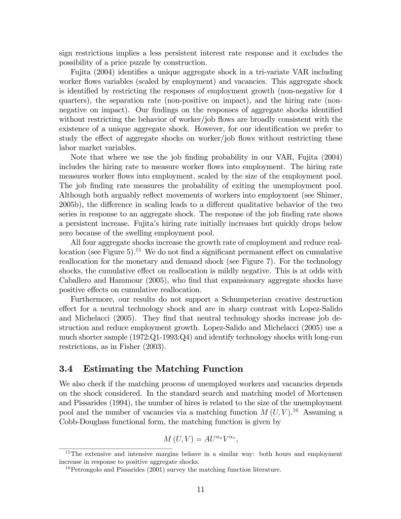
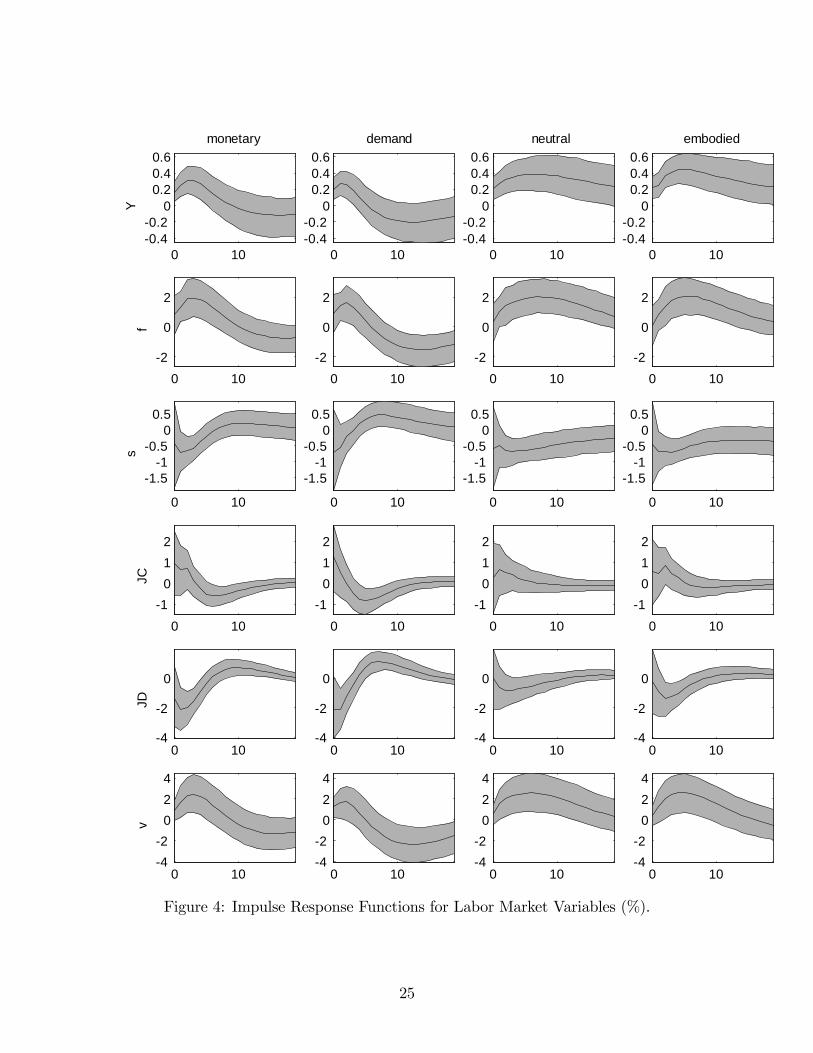
Figures 3-5 report the median, 16th, and 84th percentiles of 1,000 draws from theposterior distribution of acceptable IRFs to the structural shocks of non-labor marketvariables (restricted in our identi�cation scheme), labor market variables (on which wedo not impose any restrictions) together with output and other variables of interest.Even though we do not restrict the response of labor productivity, the IRFs of

average labor productivity to supply shocks display a persistent increase (see Figure6). Productivity shows no persistent response to demand and monetary shocks. TheIRFs of productivity suggest that the supply shocks we identify are indeed inter-pretable as technology shocks, and comparable to technology shocks identi�ed withlong-run restrictions (see Lopez-Salido and Michelacci, 2005).All labor market variables (see Figure 4) respond in a similar way to monetary

and demand shocks. Also the IRFs to neutral and embodied shocks are similar to

9

each other in shape and magnitude. Technology shocks generate responses that arequalitatively similar to those induced by monetary and demand shocks, but that havea more persistent e¤ect.The IRFs of the job �nding rate and vacancies are similar in shape to the hump-

shaped response of output for all shocks. The separation rate IRFs to the variousshocks are U-shaped. The largest e¤ect is reached earlier for the separation rate thanfor the job �nding rate. The job �nding rate responds about twice as much as theseparation rate for all shocks. The responses of the job destruction rate are similarin shape to those of the separation rate, but are larger in magnitude. The responsesof the job creation rate are the mirror image of the IRFs of the job destruction rate.Job destruction responds to shocks twice as much as job creation does.From the job �ows perspective, the destruction margin is more important in re-

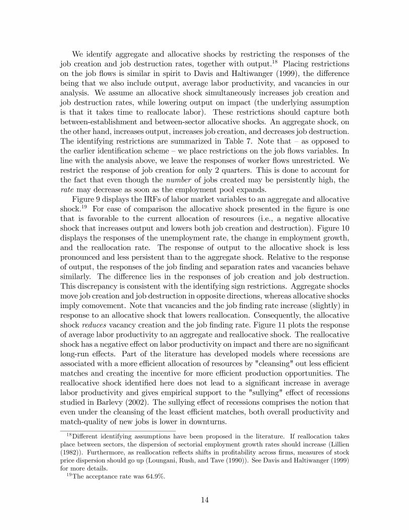
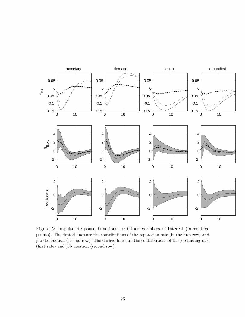
sponse to the four shocks we identify. Worker �ows�responses suggest the opposite:the creation margin is the most important. Recall, however, that the job �ndingprobability measures the exit rate from the unemployment pool, whereas the job cre-ation rate measures an entry rate into the employment pool (in terms of jobs), from�rms�perspective.Figure 5 reports the IRFs of unemployment, employment growth (implied by

equation 2), and the reallocation rate (equation 3).The unemployment rate decreases for 10 quarters in response to monetary and

demand shocks and overshoots its steady state value before converging back to it.The response of the unemployment rate decreases in a U-shaped way in response totechnology shocks. For all shocks, the response of the unemployment rate is mostlydetermined by the e¤ect on the job �nding rate, although the separation rate con-tributes up to one third of the total e¤ect. In terms of job �ows, however, the responseof employment growth is largely driven by job creation.Figure 8 reports the median of the posterior distribution of variance decomposi-

tions, i.e., the percentage of the j-periods-ahead forecast error accounted for by theidenti�ed shocks. The forecast error of output and hours is mostly driven by supplyshocks, consistent with Fisher (2003). Of the four shocks we identify, the demandshock plays the most important role in terms of the variance decomposition of job�ows. Each of the other three shocks contributes half as much as the demand shock.For worker �ows, technology shocks of either kind are the most important source ofthe forecast error variance, up to 40 quarters ahead. There is no clear pattern forvacancies.

3.3 Comparison with Existing Literature

The IRFs of job creation and destruction to a monetary shock are consistent withTrigari (2004). The di¤erences in the responses of the interest rate and of the in�ationrate stem from the di¤erent identi�cation schemes. A monetary shock identi�ed withcontemporaneous restrictions typically has a very persistent e¤ect on the interestrate and generates a price puzzle.14 Identi�cation of monetary policy shocks via

14See Altig, Christiano, Eichenbaum, and Lindé (2005) and Braun (2005).

10

sign restrictions implies a less persistent interest rate response and it excludes thepossibility of a price puzzle by construction.Fujita (2004) identi�es a unique aggregate shock in a tri-variate VAR including

worker �ows variables (scaled by employment) and vacancies. This aggregate shockis identi�ed by restricting the responses of employment growth (non-negative for 4quarters), the separation rate (non-positive on impact), and the hiring rate (non-negative on impact). Our �ndings on the responses of aggregate shocks identi�edwithout restricting the behavior of worker/job �ows are broadly consistent with theexistence of a unique aggregate shock. However, for our identi�cation we prefer tostudy the e¤ect of aggregate shocks on worker/job �ows without restricting theselabor market variables.Note that where we use the job �nding probability in our VAR, Fujita (2004)

includes the hiring rate to measure worker �ows into employment. The hiring ratemeasures worker �ows into employment, scaled by the size of the employment pool.The job �nding rate measures the probability of exiting the unemployment pool.Although both arguably re�ect movements of workers into employment (see Shimer,2005b), the di¤erence in scaling leads to a di¤erent qualitative behavior of the twoseries in response to an aggregate shock. The response of the job �nding rate showsa persistent increase. Fujita�s hiring rate initially increases but quickly drops belowzero because of the swelling employment pool.All four aggregate shocks increase the growth rate of employment and reduce real-

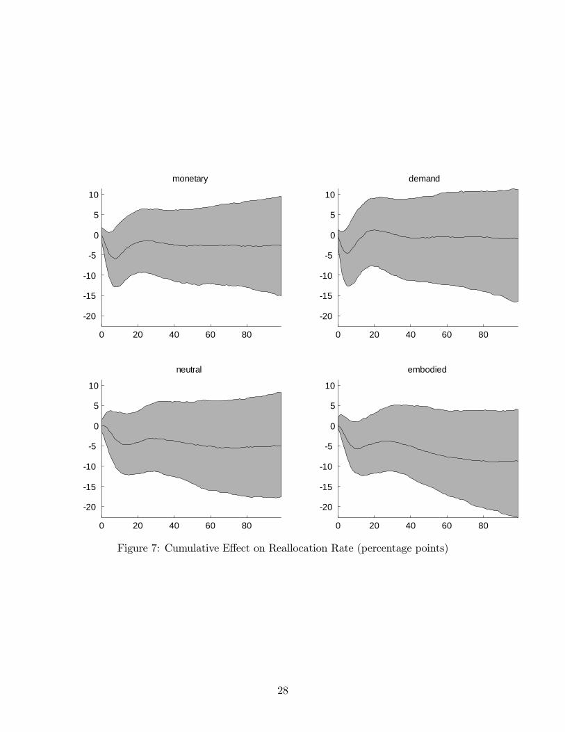
location (see Figure 5).15 We do not �nd a signi�cant permanent e¤ect on cumulativereallocation for the monetary and demand shock (see Figure 7). For the technologyshocks, the cumulative e¤ect on reallocation is mildly negative. This is at odds withCaballero and Hammour (2005), who �nd that expansionary aggregate shocks havepositive e¤ects on cumulative reallocation.Furthermore, our results do not support a Schumpeterian creative destruction

e¤ect for a neutral technology shock and are in sharp contrast with Lopez-Salidoand Michelacci (2005). They �nd that neutral technology shocks increase job de-struction and reduce employment growth. Lopez-Salido and Michelacci (2005) use amuch shorter sample (1972:Q1-1993:Q4) and identify technology shocks with long-runrestrictions, as in Fisher (2003).

3.4 Estimating the Matching Function

We also check if the matching process of unemployed workers and vacancies dependson the shock considered. In the standard search and matching model of Mortensenand Pissarides (1994), the number of hires is related to the size of the unemploymentpool and the number of vacancies via a matching function M (U; V ).16 Assuming aCobb-Douglass functional form, the matching function is given by

M (U; V ) = AU�uV �v ;

15The extensive and intensive margins behave in a similar way: both hours and employmentincrease in response to positive aggregate shocks.16Petrongolo and Pissarides (2001) survey the matching function literature.

11

where �v is the elasticity of the number of matches with respect to vacancies andmeasures the positive externality caused by �rms on searching workers; �u is theelasticity with respect to unemployment and measures the positive externality fromworkers to �rms; A captures the overall e¢ ciency of the matching function.Under the assumption of constant returns to scale (CRS), the job �nding rate can

then be expressed as:ln ft = lnA+ � (ln vt � lnut) : (7)

If we do not impose CRS, we get:

ln ft = lnA+ �v ln vt � (1� �u) ln ut:To consider the e¤ect of the shocks we identi�ed on the matching function, we

consider a sample of 1,000 draws from the posterior distributions of A and the elas-ticity parameters estimated from arti�cial data. Each draw involves the followingsteps:

1. Consider a vector of accepted residuals as if the shock(s) of interest were theonly structural shock(s);

2. Use this vector of accepted residuals and the VAR coe¢ cients from the invertedWishart-Normal family (5)� (6) to generate arti�cial data ~Zt;

3. Construct unemployment using the steady state approximation ~ut+1 = ~st=�~st + ~ft

�from the arti�cial data;

4. Regress ln ~ft on either ln vt and lnut (not assuming CRS) or ln (~vt=~ut) (underthe CRS assumption).

The arti�cial data constructed using only monetary shocks, for example, inducea posterior distribution for � and A for an hypothetical economy in which monetaryshocks are the only source of �uctuations.Table 4 reports the median, 16th, and 84th percentiles of 1,000 draws from the

posterior distributions. The �rst two columns show the estimates for �v and A whenwe impose CRS. The CRS estimates suggest that aggregate shocks do not entail adi¤erential e¤ect on the matching process. The estimated e¢ ciency parameters Aare somewhat lower for monetary and demand shocks than for technology shocks,but these median estimates di¤er by not more than 5% and the median estimates for�v are similar. The last three columns of Table 4 show the unrestricted estimates for�v, �u, and A. Not imposing CRS leads to a di¤erent picture. Estimates of �v and �uacross the shocks are close but the sum of the coe¢ cients is around 0.70, correspondingto decreasing returns to scale. There is a bigger di¤erence in the median estimates ofthe e¢ ciency parameter. A is more than a quarter higher in the case of the demandversus the embodied shock (1.10 compared with 0.86). This suggests matching occursmore e¢ ciently in the wake of monetary and demand shocks than after technologyshocks.

12

3.5 Subsample Stability

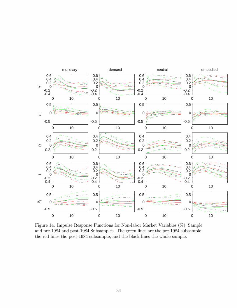
A number of papers have documented the large drop in the volatility of output,in�ation, interest rates, and many other macroeconomic variables since the mid-1980s.Motivated by the results of this literature, we now break our sample in a pre-1984and post-1984 period (see, e.g., Kim and Nelson (1999)). Figures 13 and 14 presentthe impulse responses of the variables in our system for the pre-1984 and post-1984period, respectively. In general, the post-1984 responses are smaller than the pre-84and whole sample responses. This seems the case across all shocks. Given that wenormalize the shocks (impulse response to one standard deviation), this is consistentwith the Great Moderation literature.Tables 5 and 6 present the matching function estimates for the two subperiods.

Three results are noteworthy: First, estimates of the elasticities �v and �u for thedi¤erent shocks are relatively close within each sample. Second, if we do not imposeCRS, all estimates for the pre-1984 sample show decreasing returns to scale. This isconsistent with the results for the full sample discussed above. If we turn to the post-1984 sample, all estimates of �v and �u suggest strongly decreasing returns to scale(sum of both elasticities around 0.40). The elasticity of the job �nding probabilitywith respect to unemployment, �(1��u), more than doubled for some shocks in thepost-1984 sample. Petrongolo and Pissarides (2001) de�ne this elasticity �u � 1 asthe negative externality (congestion) caused by the unemployed on other unemployedworkers. We �nd this negative externality doubled in the case of some shock forthe post-1984 sample. Likewise Petrongolo and Pissarides (2001) de�ne �v � 1 asthe negative externality placed by �rms on each other. This measure fell as well.The lower elasticity estimates for both �v and �u in the later period indicate morecongestion and less-positive externalities on the labor market. Third, there has beena substantial shift in the relative e¢ ciency of the matching function following moneyand demand shocks versus the two technology shocks. In the pre-1984 sample themedian estimate of A in an economy with, for example, only monetary shocks ismore than four times higher than the median estimate after an embodied shock. Thisrelative e¢ ciency is much lower in the post-1984 sample: the estimate for A in thecase of the monetary shock is only half as high as the estimate for the embodiedshock.

3.6 Reallocation Shocks

Although the shocks identi�ed above have an impact on reallocation, their identi-�cation is based on an aggregate shock interpretation. This section proposes analternative SVAR to assess the e¤ect of a purely allocative shock. The exact rolesuch an allocative shock plays has been a recurrent question in the study of the labormarket over the business cycle.17 Reallocation of labor across employment opportu-nities could be induced by demand shifts (primarily between sectors) or technologicalinnovations (primarily between �rms or establishments).

17See Davis and Haltiwanger (1992) and Davis and Haltiwanger (1999).

13

We identify aggregate and allocative shocks by restricting the responses of thejob creation and job destruction rates, together with output.18 Placing restrictionson the job �ows is similar in spirit to Davis and Haltiwanger (1999), the di¤erencebeing that we also include output, average labor productivity, and vacancies in ouranalysis. We assume an allocative shock simultaneously increases job creation andjob destruction rates, while lowering output on impact (the underlying assumptionis that it takes time to reallocate labor). These restrictions should capture bothbetween-establishment and between-sector allocative shocks. An aggregate shock, onthe other hand, increases output, increases job creation, and decreases job destruction.The identifying restrictions are summarized in Table 7. Note that �as opposed tothe earlier identi�cation scheme �we place restrictions on the job �ows variables. Inline with the analysis above, we leave the responses of worker �ows unrestricted. Werestrict the response of job creation for only 2 quarters. This is done to account forthe fact that even though the number of jobs created may be persistently high, therate may decrease as soon as the employment pool expands.Figure 9 displays the IRFs of labor market variables to an aggregate and allocative

shock.19 For ease of comparison the allocative shock presented in the �gure is onethat is favorable to the current allocation of resources (i.e., a negative allocativeshock that increases output and lowers both job creation and destruction). Figure 10displays the responses of the unemployment rate, the change in employment growth,and the reallocation rate. The response of output to the allocative shock is lesspronounced and less persistent than to the aggregate shock. Relative to the responseof output, the responses of the job �nding and separation rates and vacancies behavesimilarly. The di¤erence lies in the responses of job creation and job destruction.This discrepancy is consistent with the identifying sign restrictions. Aggregate shocksmove job creation and job destruction in opposite directions, whereas allocative shocksimply comovement. Note that vacancies and the job �nding rate increase (slightly) inresponse to an allocative shock that lowers reallocation. Consequently, the allocativeshock reduces vacancy creation and the job �nding rate. Figure 11 plots the responseof average labor productivity to an aggregate and reallocative shock. The reallocativeshock has a negative e¤ect on labor productivity on impact and there are no signi�cantlong-run e¤ects. Part of the literature has developed models where recessions areassociated with a more e¢ cient allocation of resources by "cleansing" out less e¢ cientmatches and creating the incentive for more e¢ cient production opportunities. Thereallocative shock identi�ed here does not lead to a signi�cant increase in averagelabor productivity and gives empirical support to the "sullying" e¤ect of recessionsstudied in Barlevy (2002). The sullying e¤ect of recessions comprises the notion thateven under the cleansing of the least e¢ cient matches, both overall productivity andmatch-quality of new jobs is lower in downturns.

18Di¤erent identifying assumptions have been proposed in the literature. If reallocation takesplace between sectors, the dispersion of sectorial employment growth rates should increase (Lillien(1982)). Furthermore, as reallocation re�ects shifts in pro�tability across �rms, measures of stockprice dispersion should go up (Loungani, Rush, and Tave (1990)). See Davis and Haltiwanger (1999)for more details.19The acceptance rate was 64.9%.

14

Figure 12 shows the cumulative responses of the reallocation rate for both theaggregate and allocative shocks. Following a positive aggregate shock, cumulativereallocation falls, then gradually recovers and stays below average. Caballero andHammour (2005) �nd that positive aggregate shocks cumulatively result in increasedrather than reduced reallocation (or restructuring). Our results suggest that cumula-tive reallocation is lower following a positive aggregate shock. Cumulative reallocationincreases following the allocative shock, as de�ned in Table 7, and does not recover.

4 Conclusion

In this paper we carry out a joint analysis of aggregate data on job and worker �owsto get a detailed view of the business cycle behavior of the postwar U.S. labor market.We report business cycle moments and calculate the dynamic response of the key labormarket variables to aggregate shocks in a set of structural vector autoregressions.Unconditional business cycle moments show that worker and job �ows data paint

somewhat di¤erent pictures of the labor market. In terms of relative volatilitiesfor example, job destruction is one-and-a-half times more volatile than job creation,whereas the separation rate is half as volatile as the job �nding rate. This discrepancyalso emerges in the dynamic response of these variables to aggregate shocks. The job�nding rate largely drives the response of unemployment whereas the separation rateexplains up to one third of unemployment �uctuations. For the job �ows data, onthe other hand, the destruction margin is more important than the creation marginin driving employment growth. These observations integrate and con�rm the resultsof other recent studies. We consider this evidence in favor of labor market modelswhere the hiring or separation decision is modeled explicitly.In terms of responses to di¤erent aggregate shocks, our main conclusion is that

worker and job �ows variables, qualitatively, behave very similarly. We do �nd thattechnology shocks generate more persistent e¤ects. Monetary and demand shocksdo not have signi�cant e¤ects on cumulative job reallocation, while expansionarytechnology shocks have mildly negative e¤ects on cumulative reallocation. Estimatesof the matching function corroborate the approach of existing search and matchingmodels in that shocks imply similar matching elasticties. On the other hand, weobserve substantial subsample shifts in both the estimates of these elasticities andthe relative shock-speci�c e¢ ciency of the matching function. Understanding whatdrives these shifts could clarify the interaction of the labor market with the observeddrop in aggregate volatility since the mid 1980s.

15

References

Abowd, J. M., and A. Zellner (1985): �Estimating Gross Labor-Force Flows,�Journal of Business and Economic Statistics, 3(3), 254�83.

Altig, D., L. J. Christiano, M. S. Eichenbaum, and J. Lindé (2005): �Firm-Speci�c Capital, Nominal Rigidities and the Business Cycle,�NBER WP 11034.

Barlevy, G. (2002): �The Sullying E¤ect of Recessions,�Review of Economic Stud-ies, 69(1), 65�96.

Blanchard, O. J., and P. Diamond (1990): �The Cyclical Behavior of the GrossFlows of U S Workers,�Brookings Papers on Economic Activity, 0(2), 85�143.

Bleakley, H., A. E. Ferris, and J. C. Fuhrer (1999): �New Data on WorkerFlows during Business Cycles,�Federal Reserve Bank of Boston New England Eco-nomic Review, pp. 49�76.

Braun, H. (2005): �(Un)Employment Dynamics: The Case of Monetary PolicyShocks,�unpublished manuscript, Northwestern.

Caballero, R. J., and M. L. Hammour (2005): �The Cost of Recessions Revis-ited: A Reverse-Liquidationist View,�Review of Economic Studies, 72(2), 313�341.

Canova, F., and G. De Nicolò (2002): �Monetary disturbances matter for busi-ness �uctuations in the G-7,�Journal of Monetary Economics, 49(6), 1131�1159.

Davis, S. J. (2005): �Comments on "Job Loss, Job Finding, and Unemployment inthe U.S. Economy over the Past Fifty Years",�in NBER Macroeconomics Annual2005, Vol. 20, ed. by M. Gertler, and K. Rogo¤. The MIT Press, Boston, MA,forthcoming.

Davis, S. J., R. J. Faberman, and J. Haltiwanger (2005): �The Flow Ap-proach to Labor Markets: New Data Sources, Micro-Macro Links and the RecentDownturn,�Discussion Paper 1639, Institute for the Study of Labor (IZA).

Davis, S. J., and J. Haltiwanger (1999): �On the Driving Forces behind CyclicalMovements in Employment and Job Reallocation,�American Economic Review,89(5), 1234�58.

Davis, S. J., and J. C. Haltiwanger (1992): �Gross Job Creation, Gross Job De-struction, and Employment Reallocation,�Quarterly Journal of Economics, 107(3),819�63.

Davis, S. J., J. C. Haltiwanger, and S. Schuh (1996): Job creation and de-struction. The MIT Press, Boston, MA.

Dedola, L., and S. Neri (2004): �What Does A Technology Shock Do? A VARAnalysis with Model-based Sign Restrictions,� forthcoming Journal of MonetaryEconomics.

16

Faberman, R. J. (2004): �Gross Job Flows over the Past Two Business Cycles: Notall �Recoveries�are Created Equal,�Discussion Paper 372, U.S. Bureau of LaborStatistics.

Fisher, J. D. M. (2003): �Technology shocks matter,�Discussion Paper WP-02-14,Federal Reserve Bank of Chicago.

Fujita, S. (2004): �Vacancy persistence,� Federal Reserve Bank of Philadelphia,Working Paper No. 04-23.

Hall, R. E. (2005a): �Employment E¢ ciency and Sticky Wages: Evidence fromFlows in the Labor Market,�Review of Economics and Statistics, 87(3), 397�407.

(2005b): �Job Loss, Job Finding, and Unemployment in the U.S. Economyover the Past Fifty Years,� in NBER Macroeconomics Annual 2005, Vol. 20, ed.by M. Gertler, and K. Rogo¤. The MIT Press, Boston, MA, forthcoming.

Jeffreys, H. (1961): Theory of Probability. Oxford University Press, London, 3rdedn.

Kim, C.-J., and C. R. Nelson (1999): �Has The U.S. Economy Become More Sta-ble? A Bayesian Approach Based On A Markov-Switching Model Of The BusinessCycle,�The Review of Economics and Statistics, 81(4), 608�616.

Lillien, D. (1982): �Sectoral Shifts and Cyclical Unemployment,�Journal of Polit-ical Economy, 90(4), 777�793.

Lopez-Salido, J. D., and C. Michelacci (2005): �Technology Shocks and JobFlows,�Discussion paper, CEMFI.

Loungani, P., M. Rush, and W. Tave (1990): �Stock Market Dispersion andUnemployment,�Journal of Monetary Economics, 25(4), 367�388.

McConnell, M. M., and G. Perez-Quiros (2000): �Output Fluctuations in theUnited States: What Has Changed since the Early 1980�s?,�American EconomicReview, 90(5), 1464�1476.

Mortensen, D. T., and C. A. Pissarides (1994): �Job Creation and Job De-struction in the Theory of Unemployment,�Review of Economic Studies, 61(3),397�415.

Peersman, G. (2005): �What Caused the Early Millenium Slowdown? EvidenceBased on Vector Autoregressions.,�Journal of Applied Econometrics, 20(2), 185�207.

Petrongolo, B., and C. A. Pissarides (2001): �Looking into the Black Box: ASurvey of the Matching Function,�Journal of Economic Literature, 39(2), 390�431.

17

Polivka, A., and S. Miller (1998): �The CPS after the Redesign: Refocusing theEconomic Lens,� in Labor statistics measurement issues. Studies in Income andWealth, vol. 60, ed. by J. Haltiwanger, M. E. Manser, and R. Topel, pp. 249�86.University of Chicago Press, Chicago and London, 0226314588 Collective-Volume-Article.

Polivka, A., and J. Rothgeb (1993): �Overhauling the Current Population Sur-vey: Redesigning the Questionnaire,�Monthly Labor Review, 116(9), 10�28.

Poterba, J. M., and L. H. Summers (1986): �Reporting Errors And Labor MarketDynamics,�Econometrica, 54(6), 1319�38.

Shimer, R. (2005a): �The Cyclicality of Hires, Separations, and Job-to-Job Transi-tions,�Federal Reserve Bank of St. Louis Review, 87(4), 493�508.

(2005b): �Reassessing the Ins and Outs of Unemployment,� unpublishedmanuscript, University of Chicago.

Stock, J. H., and M. W. Watson (2002): �Has the Business Cycle Changed andWhy?,�NBER Working Papers 9127, National Bureau of Economic Research, Inc.

Trigari, A. (2004): �Equilibrium unemployment, job �ows and in�ation dynamics,�European Central Bank, Working Paper No. 304.

Uhlig, H. (2005): �What are the e¤ects of monetary policy on output? Resultsfrom an agnostic identi�cation procedure,�Journal of Monetary Economics, 52(2),381�419.

18

f s JC JD u v y

f 6:51[5:85;7:32]

�0:30[�0:45;�0:13]

0:01[�0:17;0:2]

�0:46[�0:6;�0:31]

�0:92[�0:94;�0:89]

0:90[0:86;0:93]

0:83[0:77;0:88]

s 3:20[2:72;3:78]

�0:40[�0:52;�0:26]

0:65[0:56;0:72]

0:48[0:35;0:58]

�0:52[�0:61;�0:40]

�0:55[�0:64;�0:44]

JC 4:72[4:12;5:48]

�0:54[�0:69;�0:37]

0:02[�0:17;0:29]

0:09[�0:09;0:29]

0:16[�0:03;0:39]

JD 7:27[6:42;8:28]

0:48[0:34;0:60]

�0:60[�0:71;�0:48]

�0:64[�0:76;�0:5]

u 7:37[6:54;8:28]

�0:93[�0:95;�0:9]

�0:86[�0:9;�0:82]

v 8:58[8;9:36]

0:91[0:88;0:94]

y 1[NA]

Table 1: Correlation Matrix of Business-Cycle Components. 1954:Q3-2004Q2. Stan-dard deviations (relative to output) are shown on the diagonal. All series were loggedand detrended using a HP(1600) �lter. Block-bootstrapped con�dence intervals inbrackets.

Levels BC componentst

st+ft�s

�s+ftstst+ �f

stst+ft

�s�s+ft

stst+ �f

Corr(x; ut+1) 0:99[0:99;1]

0:85[0:76;0:92]

0:79[0:64;0:87]

0:98[0:96;0:98]

0:90[0:86;0:92]

0:62[0:51;0:7]

Std(x) =Std(ut+1) 1:01[1;1:03]

0:69[0:6;0:83]

0:49[0:43;0:59]

1:05[1:02;1:08]

0:81[0:75;0:9]

0:38[0:33;0:46]

Table 2: Contribution of the Job Finding and Separation Rate to Unemployment:Levels and Business Cycle Component. The business cycle component is extractedwith a HP(1600) �lter. Block-bootstrapped con�dence intervals in brackets.

19

Variable Monetary Shock Demand Shock Neutral shock Embodied Shock

Output " (4) " (4) " (4) " (4)Price Level " (4) " (4) # (4) # (4)Interest Rate # (1) " (1) # (1) # (1)Price of Investment � � � # (4)

Table 3: Sign Restrictions (duration in quarters in parentheses)

CRS no CRS�v A �v 1� �u A

Monetary 0:4[0:39;0:4]

3:50[3:35;3:54]

0:29[0:25;0:31]

0:55[0:53;0:57]

1:02[0:71;1:22]

Demand 0:39[0:38;0:41]

3:38[3:39;3:65]

0:29[0:25;0:32]

0:54[0:51;0:58]

1:10[0:71;1:4]

Neutral 0:41[0:41;0:41]

3:68[3:51;3:73]

0:27[0:25;0:30]

0:57[0:56;0:58]

0:87[0:7;1:04]

Embodied 0:41[0:40;0:41]

3:63[3:46;3:82]

0:28[0:25;0:29]

0:58[0:56;0:59]

0:86[0:7;0:99]

All 0:41[0:4;0:42]

3:70[3:59;3:72]

0:26[0:25;0:29]

0:58[0:55;0:59]

0:74[0:69;1:04]

Data 0:41[0:4;0:41]

3:59[3:41;3:62]

0:26[0:24;0:28]

0:58[0:56;0:58]

0:75[0:67;0:96]

Table 4: Matching Function Estimates: Elasticities and Matching E¢ ciency. Medianof the posterior distribution; 16th and 84th percentiles in parenthesis.

Pre 84 CRS no CRS�v A �v 1� �u A

Monetary 0:39[0:39;0:4]

3:49[3:41;3:65]

0:49[0:46;0:52]

0:3[0:27;0:32]

8:98[6:92;12:44]

Demand 0:4[0:4;0:41]

3:60[3:48;3:78]

0:47[0:4;0:54]

0:33[0:26;0:4]

6:98[3:54;14:73]

Neutral 0:44[0:43;0:45]

4:32[4:08;4:45]

0:39[0:32;0:46]

0:49[0:42;0:52]

2:55[1:45;5:3]

Embodied 0:42[0:41;0:43]

3:85[3:66;4:01]

0:36[0:32;0:44]

0:48[0:42;0:49]

2:1[1:55;4:35]

All 0:41[0:41;0:42]

3:77[3:66;4:05]

0:35[0:33;0:41]

0:48[0:45;0:49]

1:93[1:7:3:3]

Data 0:41[0:41;0:42]

3:75[3:71;3:94]

0:36[0:32;0:41]

0:46[0:42;0:51]

2:16[1:44;3:72]

Table 5: Matching Function Estimates Pre 1984: Elasticities and Matching E¢ ciency.Median of the posterior distribution; 16th and 84th percentiles in parenthesis

20

Post 84 CRS no CRS�v A �v 1� �u A

Monetary 0:43[0:42;0:45]

4:02[3:90;4:34]

0:21[0:16;0:23]

0:74[0:73;0:79]

0:31[0:22;0:36]

Demand 0:45[0:45;0:46]

4:52[4:39;4:66]

0:25[0:2;0:3]

0:72[0:69;0:75]

0:46[0:3;0:65]

Neutral 0:43[0:42;0:44]

3:98[3:90;4:22]

0:21[0:17;0:22]

0:78[0:74;0:81]

0:28[0:21;0:34]

Embodied 0:44[0:43;0:45]

4:32[4:02;4:39]

0:18[0:14;0:21]

0:81[0:8;0:83]

0:21[0:15;0:26]

All 0:44[0:43;0:45]

4:25[4;4:38]

0:18[0:17;0:2]

0:81[0:81;0:85]

0:2[0:19;0:23]

Data 0:44[0:42;0:45]

4:26[3:87;4:38]

0:18[0:17;0:19]

0:84[0:83;0:87]

0:2[0:17;0:21]

Table 6: Matching Function Estimates Post 1984: Elasticities and Matching E¢ -ciency. Median of the posterior distribution; 16th and 84th percentiles in parenthesis

Variable Aggregate Shock Allocative Shock

Output " (4) # (1)Job Creation " (2) " (2)Job Destruction # (3) " (3)

Table 7: Sign Restrictions for an Aggregate and Allocative Shock (duration in quartersin parentheses)

21

Q3­54 Q4­62 Q1­71 Q2­79 Q3­87 Q4­95 Q1­04

­0.9

­0.8

­0.7

­0.6

­0.5

­0.4

­0.3

­0.2

log(ft)

Q3­54 Q4­62 Q1­71 Q2­79 Q3­87 Q4­95 Q1­04

­0.2

­0.1

0

0.1

0.2

log(ft): BC component

Q3­54 Q4­62 Q1­71 Q2­79 Q3­87 Q4­95 Q1­04

­3.6

­3.5

­3.4

­3.3

­3.2

­3.1

­3

log(st)

Q3­54 Q4­62 Q1­71 Q2­79 Q3­87 Q4­95 Q1­04

­0.1

­0.05

0

0.05

0.1

0.15

log(st): BC component

Figure 1: Worker Flows: Levels and Business Cycle Components.

22

Q3­54 Q4­62 Q1­71 Q2­79 Q3­87 Q4­95 Q1­04­3.3

­3.2

­3.1

­3

­2.9

­2.8

­2.7

­2.6

log(JCt)

Q3­54 Q4­62 Q1­71 Q2­79 Q3­87 Q4­95 Q1­04

­0.2

­0.1

0

0.1

0.2

log(JCt): BC component

Q3­54 Q4­62 Q1­71 Q2­79 Q3­87 Q4­95 Q1­04­3.2

­3.1

­3

­2.9

­2.8

­2.7

­2.6

­2.5

­2.4

log(JDt)

Q3­54 Q4­62 Q1­71 Q2­79 Q3­87 Q4­95 Q1­04

­0.2

­0.1

0

0.1

0.2

0.3

0.4

log(JDt): BC component

Figure 2: Job Flows: Levels and Business Cycle Components.

23

0 10­0.4­0.2

00.20.40.6

Y

monetary

0 10­0.4­0.2

00.20.40.6

demand

0 10­0.4­0.2

00.20.40.6

neutral

0 10­0.4­0.2

00.20.40.6

embodied

0 10­0.6­0.4­0.2

00.20.4

π

0 10­0.6­0.4­0.2

00.20.4

0 10­0.6­0.4­0.2

00.20.4

0 10­0.6­0.4­0.2

00.20.4

0 10

­0.20

0.20.4

R

0 10

­0.20

0.20.4

0 10

­0.20

0.20.4

0 10

­0.20

0.20.4

0 10­0.4­0.2

00.20.40.6

l

0 10­0.4­0.2

00.20.40.6

0 10­0.4­0.2

00.20.40.6

0 10­0.4­0.2

00.20.40.6

0 10­0.6­0.4­0.2

00.20.4

p I

0 10­0.6­0.4­0.2

00.20.4

0 10­0.6­0.4­0.2

00.20.4

0 10­0.6­0.4­0.2

00.20.4

Figure 3: Impulse Response Functions for Non-Labor Market Variables (% unlessindicated otherwise).

24

0 10­0.4­0.2

00.20.40.6

Ymonetary

0 10­0.4­0.2

00.20.40.6

demand

0 10­0.4­0.2

00.20.40.6

neutral

0 10­0.4­0.2

00.20.40.6

embodied

0 10­2

0

2

f

0 10­2

0

2

0 10­2

0

2

0 10­2

0

2

0 10

­1.5­1

­0.50

0.5

s

0 10

­1.5­1

­0.50

0.5

0 10

­1.5­1

­0.50

0.5

0 10

­1.5­1

­0.50

0.5

0 10­1

012

JC

0 10­1

012

0 10­1

012

0 10­1

012

0 10­4

­2

0

JD

0 10­4

­2

0

0 10­4

­2

0

0 10­4

­2

0

0 10­4­2

024

v

0 10­4­2

024

0 10­4­2

024

0 10­4­2

024

Figure 4: Impulse Response Functions for Labor Market Variables (%).

25

0 10­0.15

­0.1

­0.05

0

0.05

u t+1

monetary

0 10­0.15

­0.1

­0.05

0

0.05

demand

0 10­0.15

­0.1

­0.05

0

0.05

neutral

0 10­0.15

­0.1

­0.05

0

0.05

embodied

0 10

­2

0

2

4

g E,t+

1

0 10

­2

0

2

4

0 10

­2

0

2

4

0 10

­2

0

2

4

0 10

­2

0

2

Rea

lloca

tion

0 10

­2

0

2

0 10

­2

0

2

0 10

­2

0

2

Figure 5: Impulse Response Functions for Other Variables of Interest (percentagepoints). The dotted lines are the contributions of the separation rate (in the �rst row) andjob destruction (second row). The dashed lines are the contributions of the job �nding rate(�rst rate) and job creation (second row).

26

0 20 40 60 80­0.4

­0.2

0

0.2

0.4

0.6

monetary

0 20 40 60 80­0.4

­0.2

0

0.2

0.4

0.6

demand

0 20 40 60 80­0.4

­0.2

0

0.2

0.4

0.6

neutral

0 20 40 60 80­0.4

­0.2

0

0.2

0.4

0.6

embodied

Figure 6: Response of Average Labor Productivity (%)

27

0 20 40 60 80

­20

­15

­10

­5

0

5

10

monetary

0 20 40 60 80

­20

­15

­10

­5

0

5

10

demand

0 20 40 60 80

­20

­15

­10

­5

0

5

10

neutral

0 20 40 60 80

­20

­15

­10

­5

0

5

10

embodied

Figure 7: Cumulative E¤ect on Reallocation Rate (percentage points)

28

0 20 405

10

15

Output

0 20 406

8

10

12

Inflation

0 20 40

5

10

15

Fed Funds

0 20 405

10

15

l

0 20 405

10

f

0 20 405

10

s

0 20 405

10

JC

0 20 40

5

10

JD

0 20 40

5

10

Vacancies

Variance Decomposition

0 20 40

5

10

Price of Investment

Figure 8: Variance Decompositions. Figure shows percentage of the j-periods aheadforecast error explained by monetary shocks (points), demand shocks (solid), neutraltechnology (dotted), embodied technology shocks (dashed).

29

0 5 10 15­0.4­0.2

00.20.40.6

Out

put

aggregate

0 5 10 15­0.4­0.2

00.20.40.6

allocative

0 5 10 15­2

0

2

f t

0 5 10 15­2

0

2

0 5 10 15­2

­1

0

s t

0 5 10 15­2

­1

0

0 5 10 15

­1012

JCt

0 5 10 15

­1012

0 5 10 15­4

­2

0

JDt

0 5 10 15­4

­2

0

0 5 10 15­4­2

024

Vac

anci

es

0 5 10 15­4­2

024

Figure 9: Aggregate versus. Allocative Shock: Impulse Response Functions for LaborMarket Variables (%). For ease of comparison the allocative shocks is presented as theshock increasing current output (i.e. a �negative� allocative shock that lowers both jobcreation and destruction).

30

0 5 10 15

­0.15

­0.1

­0.05

0

0.05

u t+1

aggregate

0 5 10 15

­0.15

­0.1

­0.05

0

0.05allocative

0 5 10 15

­2

0

2

4

6

g E,t+

1

0 5 10 15

­2

0

2

4

6

0 5 10 15

­4

­2

0

Rea

lloca

tion

0 5 10 15

­4

­2

0

Figure 10: Aggregate versus Allocative Shock: Other Variables (ppts). The dottedlines are the contributions of the separation rate (in the �rst row) and job destruction(second row). The dashed lines are the contributions of the job �nding rate (�rst row) andjob creation (second row).

31

0 20 40 60 80

­0.8

­0.6

­0.4

­0.2

0

0.2

0.4

0.6

aggregate

0 20 40 60 80

­0.8

­0.6

­0.4

­0.2

0

0.2

0.4

0.6

allocative

Figure 11: Aggregate versus Reallocative Shock: Response of Average Labor Produc-tivity (%). The allocative shocks is presented as the shock increasing current output (i.e.a �negative�allocative shock that lowers both job creation and destruction).

0 20 40 60 80

­20

­15

­10

­5

0

5

aggregate

0 20 40 60 80

­20

­15

­10

­5

0

5

allocative

Figure 12: Cumulative E¤ect on Reallocation Rate (ppts). The allocative shocks ispresented as the shock increasing current output (i.e. a �negative� allocative shock thatlowers both job creation and destruction).

32

0 10­0.4­0.2

00.20.40.6

Ymonetary

0 10­0.4­0.2

00.20.40.6

demand

0 10­0.4­0.2

00.20.40.6

neutral

0 10­0.4­0.2

00.20.40.6

embodied

0 10­2

0

2

f

0 10­2

0

2

0 10­2

0

2

0 10­2

0

2

0 10

­1

0

1

s

0 10

­1

0

1

0 10

­1

0

1

0 10

­1

0

1

0 10

­1012

JC

0 10

­1012

0 10

­1012

0 10

­1012

0 10­4

­2

0

2

JD

0 10­4

­2

0

2

0 10­4

­2

0

2

0 10­4

­2

0

2

0 10­4­2

024

v

0 10­4­2

024

0 10­4­2

024

0 10­4­2

024

Figure 13: Impulse Response Functions for Labor Market Variables (%): Sample andpre-1984 and post-1984 Subsamples. The green lines are the pre-1984 subsample, thered lines the post-1984 subsample, and the black lines the whole sample.

33

0 10­0.4­0.2

00.20.40.6

Y

monetary

0 10­0.4­0.2

00.20.40.6

demand

0 10­0.4­0.2

00.20.40.6

neutral

0 10­0.4­0.2

00.20.40.6

embodied

0 10

­0.5

0

0.5

π

0 10

­0.5

0

0.5

0 10

­0.5

0

0.5

0 10

­0.5

0

0.5

0 10

­0.20

0.20.4

R

0 10

­0.20

0.20.4

0 10

­0.20

0.20.4

0 10

­0.20

0.20.4

0 10­0.4­0.2

00.20.40.6

l

0 10­0.4­0.2

00.20.40.6

0 10­0.4­0.2

00.20.40.6

0 10­0.4­0.2

00.20.40.6

0 10

­0.5

0

0.5

p I

0 10

­0.5

0

0.5

0 10

­0.5

0

0.5

0 10

­0.5

0

0.5

Figure 14: Impulse Response Functions for Non-labor Market Variables (%): Sampleand pre-1984 and post-1984 Subsamples. The green lines are the pre-1984 subsample,the red lines the post-1984 subsample, and the black lines the whole sample.

34

Variable Units Haver (USECON)

Civilian Noninstitutional Population Thousands LN16NReal GDP Bil. Chn. 2000 $, SAAR GDPHGDP: Chain Price Index Index, 2000=100, SA JGDPFederal Funds (e¤ective) Rate % p.a. FFEDHours of all persons (Nonfarm Bus. Sector) Index, 1992=100, SA LXFNHIndex of Help-Wanted Advertising in Newpapers Index, 1987=100, SA LHELPCivilian Labor Force (16yrs +) Thoursands, SA LFCivilian Unemployment Rate (16yrs +) %, SA LR

Table A.1: Raw data

A Data

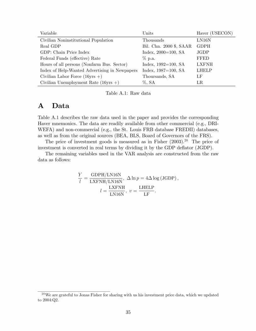
Table A.1 describes the raw data used in the paper and provides the correspondingHaver mnemonics. The data are readily available from other commercial (e.g., DRI-WEFA) and non-commercial (e.g., the St. Louis FRB database FREDII) databases,as well as from the original sources (BEA, BLS, Board of Governors of the FRS).The price of investment goods is measured as in Fisher (2003).20 The price of

investment is converted in real terms by dividing it by the GDP de�ator (JGDP).The remaining variables used in the VAR analysis are constructed from the raw

data as follows:

Y

l=

GDPH/LN16N

LXFNH/LN16N; � ln p = 4� log (JGDP) ;

l =LXFNH

LN16N; v =

LHELP

LF:

20We are grateful to Jonas Fisher for sharing with us his investment price data, which we updatedto 2004:Q2.

35

B Measuring Short-term Unemployment

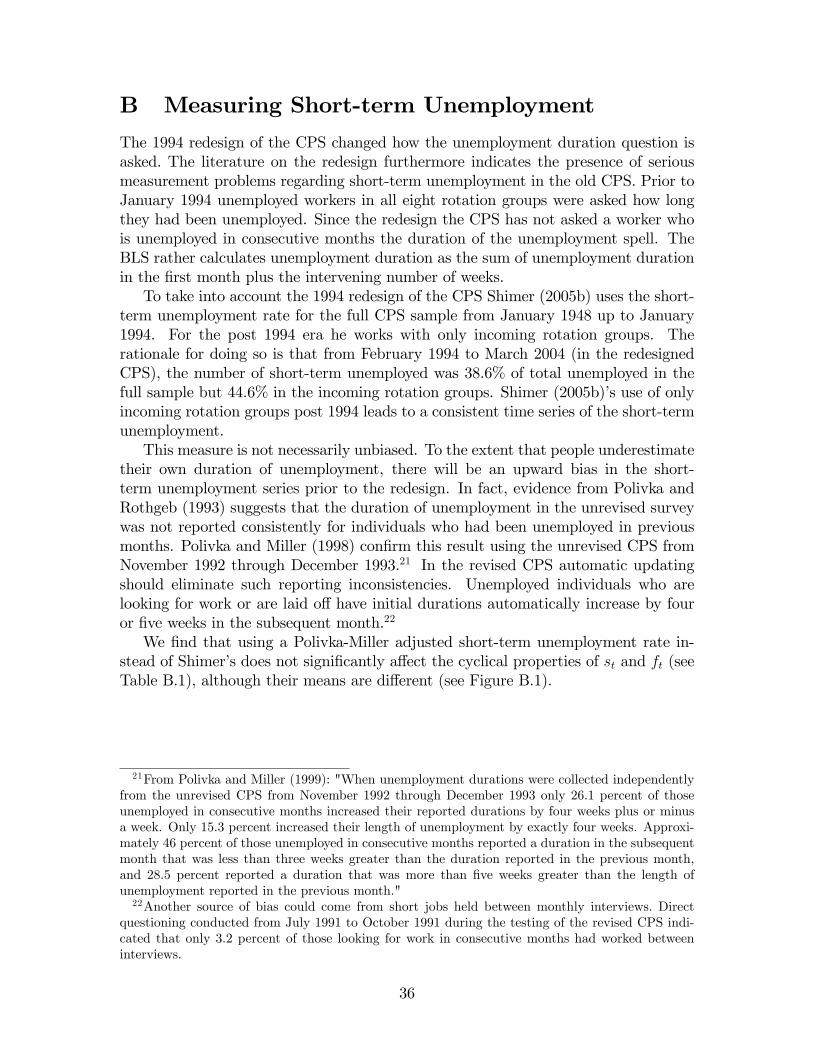
The 1994 redesign of the CPS changed how the unemployment duration question isasked. The literature on the redesign furthermore indicates the presence of seriousmeasurement problems regarding short-term unemployment in the old CPS. Prior toJanuary 1994 unemployed workers in all eight rotation groups were asked how longthey had been unemployed. Since the redesign the CPS has not asked a worker whois unemployed in consecutive months the duration of the unemployment spell. TheBLS rather calculates unemployment duration as the sum of unemployment durationin the �rst month plus the intervening number of weeks.To take into account the 1994 redesign of the CPS Shimer (2005b) uses the short-

term unemployment rate for the full CPS sample from January 1948 up to January1994. For the post 1994 era he works with only incoming rotation groups. Therationale for doing so is that from February 1994 to March 2004 (in the redesignedCPS), the number of short-term unemployed was 38.6% of total unemployed in thefull sample but 44.6% in the incoming rotation groups. Shimer (2005b)�s use of onlyincoming rotation groups post 1994 leads to a consistent time series of the short-termunemployment.This measure is not necessarily unbiased. To the extent that people underestimate

their own duration of unemployment, there will be an upward bias in the short-term unemployment series prior to the redesign. In fact, evidence from Polivka andRothgeb (1993) suggests that the duration of unemployment in the unrevised surveywas not reported consistently for individuals who had been unemployed in previousmonths. Polivka and Miller (1998) con�rm this result using the unrevised CPS fromNovember 1992 through December 1993.21 In the revised CPS automatic updatingshould eliminate such reporting inconsistencies. Unemployed individuals who arelooking for work or are laid o¤ have initial durations automatically increase by fouror �ve weeks in the subsequent month.22

We �nd that using a Polivka-Miller adjusted short-term unemployment rate in-stead of Shimer�s does not signi�cantly a¤ect the cyclical properties of st and ft (seeTable B.1), although their means are di¤erent (see Figure B.1).

21From Polivka and Miller (1999): "When unemployment durations were collected independentlyfrom the unrevised CPS from November 1992 through December 1993 only 26.1 percent of thoseunemployed in consecutive months increased their reported durations by four weeks plus or minusa week. Only 15.3 percent increased their length of unemployment by exactly four weeks. Approxi-mately 46 percent of those unemployed in consecutive months reported a duration in the subsequentmonth that was less than three weeks greater than the duration reported in the previous month,and 28.5 percent reported a duration that was more than �ve weeks greater than the length ofunemployment reported in the previous month."22Another source of bias could come from short jobs held between monthly interviews. Direct

questioning conducted from July 1991 to October 1991 during the testing of the revised CPS indi-cated that only 3.2 percent of those looking for work in consecutive months had worked betweeninterviews.

36

fShimer sShimer fPM sPM u v y

fShimer 6:51[5:8;7:3]

�0:30[�0:45;�0:15]

0:98[0:96;0:99]

�0:45[�0:57;�0:31]

�0:92[�0:94;�0:89]

0:90[0:86;0:93]

0:83[0:77;0:88]

sShimer 3:20[2:7;3:8]

�0:33[�0:47;�0:18]

0:93[0:89;0:96]

0:48[0:37;0:58]

�0:52[�0:61;�0:42]

�0:55[�0:64;�0:45]

fPM 5:68[5:1;6:4]

�0:41[�0:54;�0:26]

�0:89[�0:92;�0:85]

0:88[0:84;0:91]

0:82[0:75;0:86]

sPM 3:34[2:9;3:9]

0:59[0:5;0:67]

�0:62[�0:69;�0:53]

�0:64[�0:71;�0:55]

u 7:37[6:6;8:3]

�0:93[�0:95;�0:9]

�0:86[�0:9;�0:83]

v 8:58[8;9:3]

0:91[0:88;0:94]

y 1[NA]

Table B.1: Correlation Matrix of Business-Cycle Components. 1954:Q3-2004Q2.Standard deviations are shown on the diagonal. All series were logged and detrendedusing a HP(1600) �lter. Block-bootstrapped con�dence intervals in brackets.

Q3­54 Q4­60 Q1­67 Q2­73 Q3­79 Q4­85 Q1­92 Q2­98

­3.8

­3.7

­3.6

­3.5

­3.4

­3.3

­3.2

­3.1

­3Separation rate (log)

Q3­54 Q4­60 Q1­67 Q2­73 Q3­79 Q4­85 Q1­92 Q2­98

­1

­0.9

­0.8

­0.7

­0.6

­0.5

­0.4

­0.3

­0.2

Hiring rate (log)

Figure B.1: Job Finding and Separation Rate: Shimer us (-) versus Polivka-Millerus(.-).

37

fShimer sShimer �UE �EU �UEAZ �EUAZ y

fShimer 6:47[5:6;7:5]

�0:24[�0:37;�0:06]

0:87[0:8;0:91]

�0:58[�0:67;�0:44]

0:87[0:8;0:9]

�0:63[�0:71;�0:5]

0:83[0:76;0:89]

sShimer 3:08[2:5;4]

�0:23[�0:38;�0:08]

0:68[0:56;0:75]

�0:22[�0:36;�0:07]

0:68[0:57;0:75]

�0:50[�0:59;�0:38]

�UE 6:08[5:3;7:2]

�0:41[�0:51;�0:25]

1:00[1;1]

�0:47[�0:56;�0:32]

0:74[0:63;0:81]

�EU 4:80[4;5:8]

�0:40[�0:50;�0:24]

1:00[1;1]

�0:71[�0:78;�0:62]

�UEAZ 5:68[5;6:7]

�0:45[�0:55;�0:31]

0:73[0:61;0:8]

�EUAZ 4:98[4:2;6]

�0:75[�0:8;�0:67]

y 1[NA]

Table C.1: Correlation Matrix of Business-Cycle Components. 1967:Q1-2004Q2.Standard deviations are shown on the diagonal. All series were logged and detrendedusing a HP(1600) �lter. Block-bootstrapped con�dence intervals in brackets.

C 3-Pools Data

The identi�cation of the job �nding and separation rates ft and st above assumes thatall workers are either unemployed or employed. Transitions into and out of the laborforce are not accounted for. We use gross worker �ows data from the CPS to checkif such a simpli�cation is defendable at the business cycle frequency. Unfortunatelythe three-pool data are only available from June 1967 onwards. As in Shimer (2005b)we compute from the gross worker �ows at time t transition rates �XYt for workerswho were in state X and moved to state Y during period t: We also consider thee¤ect of adjusting the gross �ows for spurious transitions stemming from correctionsof missclassi�cation errors in successive interviews. We use the weights from Bleakley,Ferris, and Fuhrer (1999). They are averages of the time varying factors calculatedin Abowd and Zellner (1985) for the period January 1976 to May 1986.Notice that the unemployment-to-employment (UE) transition rates are highly

correlated to the job �nding rate, and they are less volatile. The employment-to-unemployment (EU) transition rates are less correlated with the separation rate, andmore volatile. This suggest that Shimer�s job �nding and separation rates might over-state the contribution of the hiring margin to the cyclical variation of unemployment.For data availability reasons we decided to use Shimer�s data in the SVAR analysisin this paper.

38

1970 1975 1980 1985 1990 1995 2000

0.3

0.4

0.5

0.6

0.7

0.8fλUE

λUE  AZ

1970 1975 1980 1985 1990 1995 2000

0.015

0.02

0.025

0.03

0.035

0.04

0.045 sλEU

λEU AZ

Figure C.1: Hiring and UE Transition Rate; Separation and EU Transition Rate.

39

D Job versus Worker Flows Data

The job �nding and separation rates focus on the unemployment pool. Ignoringthe time aggregation adjustment, the job �nding rate rate is equal to the numberof unemployed workers who found a job within a period scaled by the size of theunemployment pool. The job �ows data, on the other hand, captures the total �owsinto employment, where both job creation and destruction are scaled by employment.Worker �ows data o¤er an alternative way of representing employment in�ows

by scaling the number of workers who �nd a job in a given period by the size ofthe employment pool. If in�ows from non-participation are included, this represen-tation is analogous to the one used in job �ows data in the sense that the di¤erencebetween in�ows and out�ows yields the growth rate of employment. We take thethree-pool data from Shimer (2005b) for the shorter sample (1967:Q2-2004:Q2) andundo the time aggregation to make the data comparable to the job �ows data. Wethen construct an ins ratio from the worker �ows data as the total �ows into employ-ment from unemployment (UEt) and out-of-the-labor-force (IEt), scaled by the totalemployment stock:23

inst �UEt + IEtEt�1

: (8)

The outs ratio is the total �ows out of employment to unemployment (EUt) andout-of-labor-force (EIt), again scaled by total employment stock:

outst �EUt + EItEt�1

: (9)

Substracting equation (9) from equation (8), we de�ne the net change in employ-ment implied by worker �ows, gWE;t, as:

gWE;t �Et � Et�1Et�1

� inst � outst. (10)

The correlation of employment growth calculated from the raw �ows as in equation(10) with BLS civilian employment growth is 0:72. Adjusting the gross �ows withthe means of the factors calculated as in Abowd and Zellner (1985), increases thiscorrelation to 0:77.24 Table D.1 presents the correlation matrix of the business-cyclecomponents of the ins and outs ratio de�ned in (8) and (9). These gross �ows wereadjusted using the means of the time varying factors calculated as in Abowd andZellner (1985) from January 1976 to May 1986. This table shows that the ins andouts ratios de�ned from worker �ows have signi�cantly di¤erent cyclical propertiesfrom the job creation and destruction series. The standard deviations of the ins and

23Scaling by the average of the current and lagged employment stock as opposed to lagged totalemployment, does not change the results.24The correlation of gWE with total non-farm employment growth is 0.71. For this sample the

corresponding correlation of gJC;JDE is 0.88. The correlation of gJC;JDE with civilian employment is0.73.

40

InsAZ

EOutsAZ

EJC JD u v y

InsAZ

E2:74

[2:16;3:48]0:26

[0:06;0:46]0:36

[0:14;0:54]�0:10

[�0:27;0:09]0:42

[0:30;0:53]�0:29

[�0:4;�0:14]�0:26

[�0:41;�0:12]OutsAZ

E2:53

[2:16;3:03]�0:29

[�0:49;�0:07]0:67

[0:51;0:76]0:59

[0:47;0:68]�0:61

[�0:70;�0:46]�0:64

[�0:74;�0:50]JC 4:64

[3:85;5:63]�0:50

[�0:67;�0:27]0:01

[�0:23;0:22]0:03

[�0:20;0:28]0:10

[�0:17;0:39]

JD 7:68[6:69;8;93]

0:48[0:30;0:61]

�0:58[�0:71;�0:42]

�0:61[�0:75;�0:43]

u 7:13[6:22;8:21]

�0:95[�0:97;�0:92]

�0:87[�0:91;�0:81]

v 8:56[7:90;9:49]

0:91[0:86;0:95]

y 1:00[NA]

Table D.1: Correlations Matrix of Business-Cycle Component of the Ins and Outsto Employment and Job Creation and Destruction Series, 1967Q2-2004Q2. Standarddeviations (relative to output) are shown on the diagonal. All series were loggedand detrended using a HP �lter with weight 1600. Block-bootstrapped con�denceintervals in brackets. "AZ" is the adjusted series using the means of the time-varyingfactors calculated in Abowd and Zellner (1985) for the period January 1976 to May1986. The worker �ows are scaled by employment at time t.

outs ratio are about half the standard deviations of the job creation and destructionrates. The job creation and destruction rate are negatively correlated, whereas thecorrelation between the ins and outs ratios is positive. Furthermore, inst is negativelycorrelated with output, whereas the correlation of job creation with output is positive.We also observe that the relative volatility of inst and outst is much lower thanthe relative volatility of the hiring and separation rate. Measuring ins and outs ofemployment using worker �ows, we �nd that the outs are almost as volatile as theins.

41