Agglomeration and Growth: The effects of Commuting Costs*

Antonio Accetturo

Università Cattolica del Sacro Cuore – Milano Istituto di Teoria Economica e Metodi Quantitativi

(ITEMQ) via Necchi, 5

20100 Milano (Italy)

ph: +39 02 7234 2918 fax: +39 02 7234 2923

antonio.accetturo@unicatt.it

Abstract: In this paper we present a model of industrial location and Endogenous Growth characterised by Increasing Return to Scale (IRS), Trade costs, horizontal innovations and Commuting costs within each region. Four forces shape the industrial location and growth process: (i) Static Centripetal forces (trade costs and IRS), (ii) Static Centrifugal forces (Commuting costs, lowering net wages, and market crowding effect), (iii) Dynamic Centripetal forces (Localised knowledge spillovers) and (iv) Dynamic Centrifugal forces (Commuting costs, slowing the innovation process). Three possible outcomes (referred to as configurations) emerge in this context. Configuration (a) is characterised by the existence of a unique sustain point of trade costs under which a Core-Periphery outcome is the only stable equilibrium. This is reached when either Localized knowledge spillovers or Commuting Costs are low. Configuration (b) is characterised by a three-stage behaviour. When trade costs are high or too low, spatial dispersion occurs; while at an intermediate level of trade costs, Core-Periphery (and Income divergence) emerges. This configuration is achieved at an intermediate level of Knowledge spillovers or Commuting Costs. Configuration (c) is characterised by spatial dispersion at every level of trade costs. This occurs when Knowledge Spillovers or Commuting Costs are large. Welfare analysis shows that, even in the presence of a gap between unskilled in the Core and unskilled in the Periphery, Core-Periphery outcome might be Pareto improving if Agglomeration enhances a higher speed of the Economy. Higher growth, anyway, must be quite substantial to compensate static losses. JEL: O41, R11. *Many thanks to prof. Boggio, Vincenzo Dall’Aglio, Stefan Gruber, Antonella Nocco and the participants to the seminars/conferences in Verona, Las Vegas, Gent.

1

1. Introduction The existence of a positive relationship between spatial agglomeration of economic

activities and growth has been widely documented by economic historians (Hohenberg and

Lees, 1985), in particular in relation to the industrial revolution in Europe in the XIX century.

In this case, as growth rate sharply increased, we observe a sudden formation of industrial

clusters in the economic core of Europe. The economic core included, at the beginning of the

XX century, the Ruhr area, the North West of Italy, the North of France, Belgium and the UK

(especially the North of England). Anyway, after one hundred years, things slightly changed

and the economic core of Europe (the so-called blue banana, see Combes and Overman, 2004)

now includes: the Ruhr area, Bavaria, the North-West, the North-East and part of the Central

Italy, Austria, France, the North of Spain, Belgium, Holland and the south of England.

On the other side of the Atlantic Ocean, in the US, economic geography of industrial

location and income have changed in a more dramatic way (Holmes and Stevens, 2004). In

the 1947, manufacturing plants were mainly concentrated in the “Manufacturing Belt” (in the

North), “Piedmont Region” (in the South) and in California. In the 1999, the picture had

become quite different and manufacturing activities were basically located everywhere

(except for the Rocky Mountains area).

Moreover, in both cases, economic core expanded and income convergence among those

regions occurred (see, e.g. Combes and Overman, 2004, for Europe). This phenomenon

occurred mainly among neighbouring regions, especially in the European case, showing that a

possible process of relocation (together with income convergence) between two neighbouring

regions may occur when congestion costs rise in the core region.

The aim of this paper is to formalize a similar process, which allows for an initial period of

geographical polarization (divergence) followed by spatial diffusion of economic activities

(convergence) in a model of growth and industrial location with congestion costs. More

specifically, this paper extends the model presented by Fujita and Thisse (2002, par. 11.4)

2

allowing for the existence of congestion costs in the form of commuting “iceberg” costs in the

labour supply of skilled workers (see e.g. Murata and Thisse, 2005). Location decisions and

income levels are influenced by increasing return to scale, trade costs, localised knowledge

spillovers and congestion costs. Economic growth is achieved by a process of horizontal

innovations in the industrial sector which produces increasing varieties of the same good (see

Romer, 1990 and Grossman and Helpman, 1991). Patents (necessary to initiate the production

of a new variety) are produced by skilled workers, which are allowed to migrate from one

region to the other. Patents cannot be transferred across regions.

Four different forces shape the spatial distribution of economic activities and, hence,

regional and aggregate economic growth (Table 1).

Table 1.

Centrifugal Centripetal

Static

Commuting Costs (Lower net

wage), Market Crowding effect

Scale Economies,

Transportation Costs

Dynamic

Commuting Costs (Lower inter-temporal

spillovers)

Localized Knowledge Spillovers

(i) Static centripetal forces are due to economies of scale and transport costs. Increasing

return to scale and transport costs allow for a concentration of economic activities in one

region as the “home market” size increases when more workers decide to locate in one region.

(ii) Dynamic centripetal forces take the form of localised knowledge spillovers.

Knowledge spillovers are stronger among the skilled workers residing in the same region. As

a result, varieties are more numerous (and utility level is higher) when agglomeration occurs.

(iii) Static centrifugal forces are linked to congestion (market crowding) and commuting

costs. When agglomeration occurs, on one side, competition in the core region increases and

3

firm profits decrease and, on the other side, net wage for skilled workers decreases as labour

supply lowers and land rents increase.

(iv) Dynamic centrifugal forces take the form of lower labour supply due to congestion. In

presence of commuting costs, labour supply for the R&D sector decreases and this harms the

production of new varieties and aggregate growth.

The interaction among these four forces creates three possible configurations of the steady

state.

Configuration (a): When knowledge spillovers (commuting costs) are particularly low,

Core-Periphery always emerges and remains stable when trade costs lowers. As a result,

income divergence occurs and income inequality persists in the Steady State. This is the case

of two (culturally) distant regions like the North and the South of the World. This result is

similar to the previous models of the “Agglomeration and Growth” literature (like Fujita and

Thisse, 2002).

Configuration (b): At an intermediate value of knowledge spillovers (commuting costs),

Core-Periphery and Income divergence occur only at an intermediate level of trade costs,

while when trade costs are either too high or too low Spatial Dispersion and Income

equalisation emerge. The economy has three phases of Convergence-Divergence-

Convergence. This is the case of many European regions (countries) like the North-East of

Italy, Spain, Ireland.

Configuration (c): When knowledge spillovers (commuting costs) are high, spatial

dispersion is the only outcome and both regions always grow at the same rate.

The paper is organised as follows. Section 2 presents a brief review of the “Agglomeration

and Growth” literature. Section 3 presents the basic features of the model. In particular, in

section 3.1 we show how the internal structure of a region looks like. In section 3.2 we

present the consumers’ problem; in section 3.3, we present the producers’ problem; in section

3.4 we show the market clearing conditions and, in section 3.5, we present the migration law

4

of motion. In section 4, we present the dynamic framework of the model: i.e. the SS growth

path when skilled workers are immobile (4.1); and the SS growth path when skilled workers

are allowed to migrate (4.2). In section 5, we present the welfare impact of the emergence of a

Core-Periphery pattern. Section 6 concludes the paper. The Appendix 1 shows an exercise of

comparative statics achieved with numerical simulations. The Appendix 2 includes proofs of

the Propositions of the model.

2. Literature Review “Agglomeration and Growth” models can be grouped in two main areas: models with

workers migration and models with capital.

Few existing migration models are due to the contributions of Walz (1996 and 1997),

Baldwin and Forslid (2000) and Fujita and Thisse (2002). Walz (1996) combines expanding

variety, migration and vertical linkages. Economic integration leads to an asymmetric

outcome even if regions are initially symmetric, costless migration, anyway, leads to a bang-

bang agglomeration pattern. Walz (1997) extends his previous analysis to a three-regions

case. Baldwin and Forslid (2000) directly extend the basic Krugman (1991) model in a

dynamic framework. They show that regional integration implying freer trade of goods and a

better knowledge transmission has a stabilising effect on regional imbalances while freer trade

of goods only leads to a destabilising integration. Unfortunately, their model is quite complex

and it cannot be solved analytically. More elegant step forward from this point of view was

presented by Fujita and Thisse (2002, ch.11), in a context characterised by forward looking

migration behaviour and localised knowledge spillovers. They show that, with patent

transferability (par. 11.3), two types of Core-Periphery configuration emerge. Core-Periphery

type one (catastrophic agglomeration of R&D workers but only partial agglomeration of the

industrial sector) arise at an intermediate level of trade costs. Core-Periphery type two

(catastrophic agglomeration of both R&D workers and industrial activities) emerges as trade

5

becomes freer. When patents cannot be transferred across regions, catastrophic agglomeration

directly occurs.

Models with capital were first introduced by Baldwin (1999) and Martin and Ottaviano

(1999). Baldwin (1999) (known as Constructed Capital, CC, model in the Baldwin et al.,

2003, taxonomy) introduced geography, love for variety and trade costs in a neoclassical

framework with both capital immobility and mobility. When capital is immobile, capital

owners may have different incentive to invest in different regions, therefore trade

liberalisation is likely to create asymmetries. When capital is mobile, instead, profits are

repatriated and, therefore, symmetric equilibrium is always stable and agglomeration is never

catastrophic. Martin and Ottaviano (1999) present an endogenous growth model with capital

mobility and either purely local or purely global knowledge spillovers. The intermediate case

of partially localised knowledge spillovers is studied in Baldwin et al. (2001) where capital is

immobile. In both the models, trade liberalisation create spatial agglomeration and income

inequality. Anyway, static losses (for the peripheral workers) due to agglomeration can be

overcome by dynamic gains (due to higher growth) if knowledge spillovers are at least

partially localised. Capital mobility (as in the CC model) plays a stabilising effect and

agglomeration cannot be catastrophic. Martin and Ottaviano (2001) present a model where

vertical linkages substitute localised knowledge spillovers as dynamic centripetal force.

Basevi and Ottaviano (2002) present an “Agglomeration and Growth” model with

intermediate capital mobility. They show, starting from an agglomerated equilibrium (i.e. the

existence of an industrial district) that an industrial relocation at a low level of trade costs can

be harmful for aggregate growth because of lower knowledge spillovers.

Urban (2002) integrates a neoclassical growth model in a static economic geography model

without capital mobility. His results are quite different from the ones presented here. As trade

costs lower, neoclassical convergence occurs across regions because of the existence of

6

decreasing returns in the core region, while at a high level of transport costs, home market

effect prevails and agglomeration occurs.

Cerina and Pigliaru (2005) present a model of permanent income divergence across regions

in which Periphery’s terms of trade always worsen as agglomeration occurs due to a different

specification of individual preferences.

Summing up the common features of these models (except for Urban, 2002), trade

liberalisation is likely to create agglomeration and income divergence across regions.

Divergence can be mitigated by capital mobility, higher knowledge spillovers and market

crowding, but, agglomeration is never reversed. As Baldwin and Martin (2004) pointed out

this class of models provide a powerful explanation of the “first wave of globalisation” (i.e.

the industrialisation of the North), while they are quite weak in the explanation of the “second

wave of globalisation” (i.e. the relocation of industrial activities in the South). The reason is

that centripetal forces are always stronger than centrifugal and congestion is too weak in the

core1. The aim of this paper is to formalise a possible process of re-industrialisation and

convergence, therefore, we introduce an additional centrifugal force, in the form of

commuting. As a result, migration models (à la Fujita-Thisse) seem more suitable to explain

this issue as urban congestion usually takes the form of workers’ concentration within a city.

3. The Model

3.1 Commuting Costs and Skilled Labour Supply

Suppose there are two regions (A and B) two factors (skilled workers H and unskilled

workers L) and four goods (an industrial horizontally differentiated good, a Traditional good,

patents and land).

1 Only Baldwin et al. (2003, ch.17) tried to formalise a growth process subject to congestion costs in an “Agglomeration and Growth” framework with capital mobility. Congestion equation is quite ad hoc as it is purely instrumental to show that the Core-Periphery process may lead to too much agglomeration hampering aggregate growth. No internal structure is introduced to explain the existence of congestion costs.

7

H-workers locate in a residential area, where Research Labs locate in the centre (a Central

Business District, CBD, which can be interpreted as a Science Park) x=0 and workers

commute to the CBD to work. Each H-worker consumes one unit of land and she commutes

to the CBD to work. The total number of H-workers in the economy is H, while the total

number of unskilled workers is 2L. Without loss of generality, we normalize H=1 and

consider 2L as the relative amount of L-workers in terms of H-workers. Each region r has a

share λr of H-workers localized inside its borders and a number fixed L of L-workers. In

equilibrium, in each region, H-workers are symmetrically distributed around the CBD, on the

interval

−

2,

2rr λλ .

Labour supply is influenced by the commuting costs to the CBD. In particular, the higher

the commuting costs, the lower is labour supply and wage earned by each skilled worker.

Like Murata-Thisse (2005), we assume that commuting costs are an increasing linear function

of the distance to the CBD. In particular, labour supply for an H-worker is:

( ) xxs θ21−= (1)

where 1<θ to ensure strictly positive labour supply and x is the distance to the CBD.

The worse the infrastructural endowment (high θ) or the higher the distance to the CBD, the

lower labour supply.

Net wage for an H-worker living on the edge of her region is:

[ ] rr wθλ−1 (2)

which is an increasing function of labour supply. The closer is a worker to the CBD, the

higher is her net wage. Hence, all the H-workers living on the interval

−

2,

2rr λλ

have a

proximity rent, which is calculated as follows:

( ) ( ) ( )

∈∀−=

−=

2,0,2

2r

rrr

rr xxwsxswxRλ

λθλ (3),

8

Aggregate rent in region r is therefore:

( )2

222

2

rrrrr wdxxwALR

r

r

λθλθ

λ

λ

=−= ∫−

(4).

Land is entirely owned by L-workers living in each region. They rent their land to the H-

workers living in their region. Therefore proximity rent is transferred to the L-workers2.

Aggregate rent per capita is L

w rr

2

2λθ .

3.2 Consumers’ problem Each worker consumes both the industrial and the traditional good with Cobb-Douglas

preferences. Patents are necessary to initiate the production of each variety of the

differentiated good. L-workers work both in the industrial and traditional sectors and they are

geographically immobile. H-workers work in the R&D (patent) sector and they are allowed to

migrate from one region to the other.

Each worker is an infinitely living consumer, which maximises the following intertemporal

problem:

( )

( ) ( )∫∫

∫

∞−

∞−

∞−

=

=

0

)(

0

)(

0

..

ln max

dttIedttEe

ts

dttVeV

ltt

ltt

rl

tl

υυ

γ

(5)

where Vlr(t) is the utility level attained by consumer l in region r at time t. γ is the

subjective discount rate. El(t) is the expenditure of consumer l at time t and Il(t) is her income.

υ(t) is the instantaneous interest rate prevailing in on the capital market.

2 H-workers living close to the CBD pay a high rent for their houses. H-workers living further from CBD pay a lower rent. H-workers living on the region’s edge pay no rents for their houses. In equilibrium, net wage for H-workers is constant and equal to the net wage of the worker living on the regional edge (equation 2).

9

Utility level Vlr(t) is obtained solving the following maximization problem for each period

t:

( )

( )

( )tEdiipiqTp

ts

Tdiiq

U

lMi

T

Mi

=+

−

=

∫

∫

∈

−

−−

∈

−

)()(

..1

max 1

111

µµ

µ

µ

σσ

µµ

σσ

(6)

where T represents the consumption of the traditional good, µ is the share of current

expenditure spent on the horizontally differentiated good, M is the total mass of varieties, q(i)

is the consumption of variety i of the horizontally differentiated good and p(i) is its price. σ is

the elasticity of substitution among varieties. pT is the price of the Traditional good.

Problems (5) and (6) are solved in two consecutives steps.

In step one, consumers choose the intertemporal consumption path which drives to the

usual Euler condition:

γυ −=∂∂

)(tE

tE

l

l

(7).

Once expenditure level is chosen for each period of time, Cobb-Douglas preferences imply

that each consumer spends a constant fraction of its expenditure on each type of good. In

particular, Marshallian demands for T-good and each variety i of M-good are:

( ) (tET l )µ−= 1 (8)

( ) ( ) ( )tEPipiq lr1−−= σσµ (9)

where Pr is a price index for the industrial good equal to:

σσ

−

∈

−

= ∫

11

1)(Mi

r diipP (10).

Utility level at time t is equal to real expenditure:

10

( ) ( ) µµ −= 1

)()(

Tr

lrl

pP

tEtV (11).

Traditional good is freely traded and it is produced with a Constant Return to Scale (one to

one) production function. Therefore its price is constant across regions and it can be

normalized to one (T is the nummeraire). Industrial good is subject to transportation costs

which, as usual in the literature, take the form of the “melting iceberg”. This means that, in

order to deliver one unit of good i to region s, producers in region r must ship τ>1 units of

good i.

Mill pricing implies that price index (9) becomes:

( ) ( )σ

σσ φ−

∈

−

∈

−

+= ∫∫

11

11

sr Mis

Mirr diipdiipP (12)

where Mr is the total number of varieties produced in region r and is a measure of

free-ness (phi-ness) of trade

στφ −≡ 1

3.

Ownership structure of the economy assumes that H-workers own the initial production

assets of the economy while L-workers own the land. As a result, skilled workers receive (in

each period of time) their wage and a share of value of the initial assets, while unskilled

workers receive their wage and the per capita ALR in region r. Unskilled wage is normalised

to one in both regions, under the assumption of incomplete specialization in the T-sector.

3.3 Producers’ problem (a) Final Good Sector (Industrial/Differentiated)

The industrial good is produced under increasing return to scale (IRS) due to the presence

of a fixed cost. The fixed cost is the purchase of a patent, which is necessary to start the

production of a differentiated good. Patents last forever and each producer has a monopoly

3 When φ=1, free trade prevails, for φ=0, trade costs are infinite.

11

power on the variety she produces. The marginal cost is determined by the use of an

additional worker L, whose wage (and marginal product) is one.

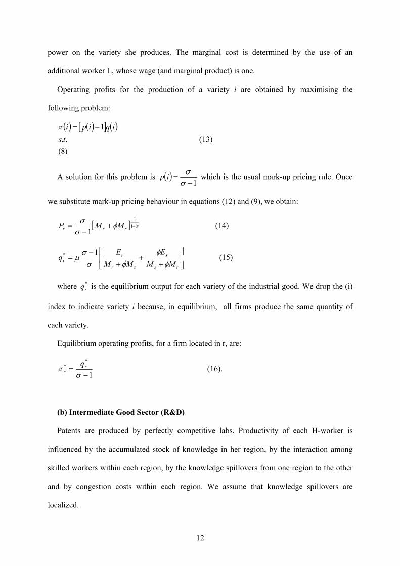
Operating profits for the production of a variety i are obtained by maximising the

following problem:

( ) ( )[ ] ( )

)8(..

1ts

iqipi −=π (13)

A solution for this problem is ( )1−

=σσip which is the usual mark-up pricing rule. Once

we substitute mark-up pricing behaviour in equations (12) and (9), we obtain:

[ ] σφσσ

−+−

= 11

1 srr MMP (14)

+

++

−=

rs

s

sr

rr MM

EMM

Eq

φφ

φσσµ 1* (15)

where is the equilibrium output for each variety of the industrial good. We drop the (i)

index to indicate variety i because, in equilibrium, all firms produce the same quantity of

each variety.

*rq

Equilibrium operating profits, for a firm located in r, are:

1

**

−=σ

π rr

q (16).

(b) Intermediate Good Sector (R&D)

Patents are produced by perfectly competitive labs. Productivity of each H-worker is

influenced by the accumulated stock of knowledge in her region, by the interaction among

skilled workers within each region, by the knowledge spillovers from one region to the other

and by congestion costs within each region. We assume that knowledge spillovers are

localized.

12

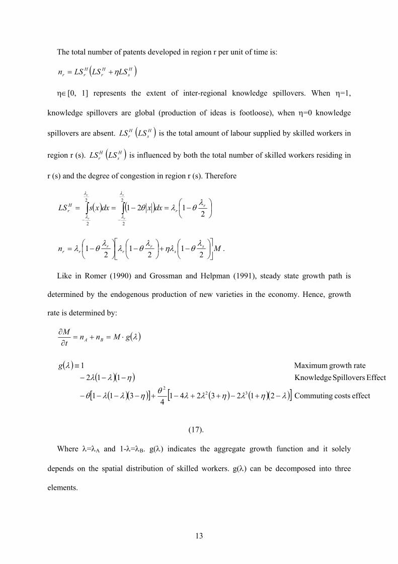
The total number of patents developed in region r per unit of time is:

( )Hs

Hr

Hrr LSLSLSn η+=

η∈[0, 1] represents the extent of inter-regional knowledge spillovers. When η=1,

knowledge spillovers are global (production of ideas is footloose), when η=0 knowledge

spillovers are absent. HrLS ( )H

sLS is the total amount of labour supplied by skilled workers in

region r (s). HrLS ( )H

sLS is influenced by both the total number of skilled workers residing in

r (s) and the degree of congestion in region r (s). Therefore

( ) ( )

−=−== ∫∫

−−2

1212

2

2

2

rr

Hr

r

r

r

r

dxxdxxsLSλ

θλθ

λ

λ

λ

λ

Mn ss

rr

rrr

−+

−

−=

21

21

21

λθηλ

λθλ

λθλ .

Like in Romer (1990) and Grossman and Helpman (1991), steady state growth path is

determined by the endogenous production of new varieties in the economy. Hence, growth

rate is determined by:

( )

( )( )( )

( )( )[ ] ( ) ( )( )[ ] effect costs Commuting 21232414

311

Effect Spillovers Knowledge 112 rategrowth Maximum 1

322

ληληλλθηλλθ

ηλλλ

λ

−+−++−+−−−−

−−−≡

⋅=+=∂∂

g

gMnnt

MBA

(17).

Where λ=λA and 1-λ=λB. g(λ) indicates the aggregate growth function and it solely

depends on the spatial distribution of skilled workers. g(λ) can be decomposed into three

elements.

13

The first is the maximum growth rate (equal to one) that can be achieved by the economy

whether localised knowledge spillovers and commuting costs are absent.

The second is the knowledge spillovers effect (KSE), according to which aggregate growth

is maximized either when skilled workers concentrate in one region (λ=1 or 0) or when

knowledge spillovers are global (η=1).

The third component represents the impact of the commuting costs effect (CCE) on the

growth rate. Commuting costs lower the aggregate growth rate especially when skilled

workers concentrate in one region only.

There is a clear trade-off between the effects of knowledge spillovers and commuting

costs on location and growth. For example, when skilled workers concentrate in one region,

KSE maximises growth rate, while CCE minimise it.

The shape of function g(λ) depends on the interplay between these two effects. In

particular, g(λ) is described by Proposition 1 and 2:

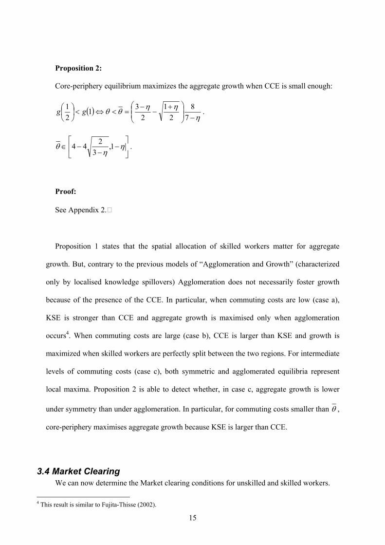
Proposition 1:

a) For η−

−≤3

244θ , g(λ) is a convex function on λ∈[0,1] with a unique minimum

in λ=1/2.

b) For ηθ −> 1 , g(λ) is a concave function with a unique maximum in λ=1/2.

c) For ηθη

−≤<−

− 13

244 , g(λ) has three local maxima in λ=0, λ=1/2 and λ=1,

and two local minima symmetric around λ=1/2. Moreover,

( )η

ηηθθ−

+−

−=≥⇔≥

78

21

231

21 gg

Proof:

See Appendix 2.

14

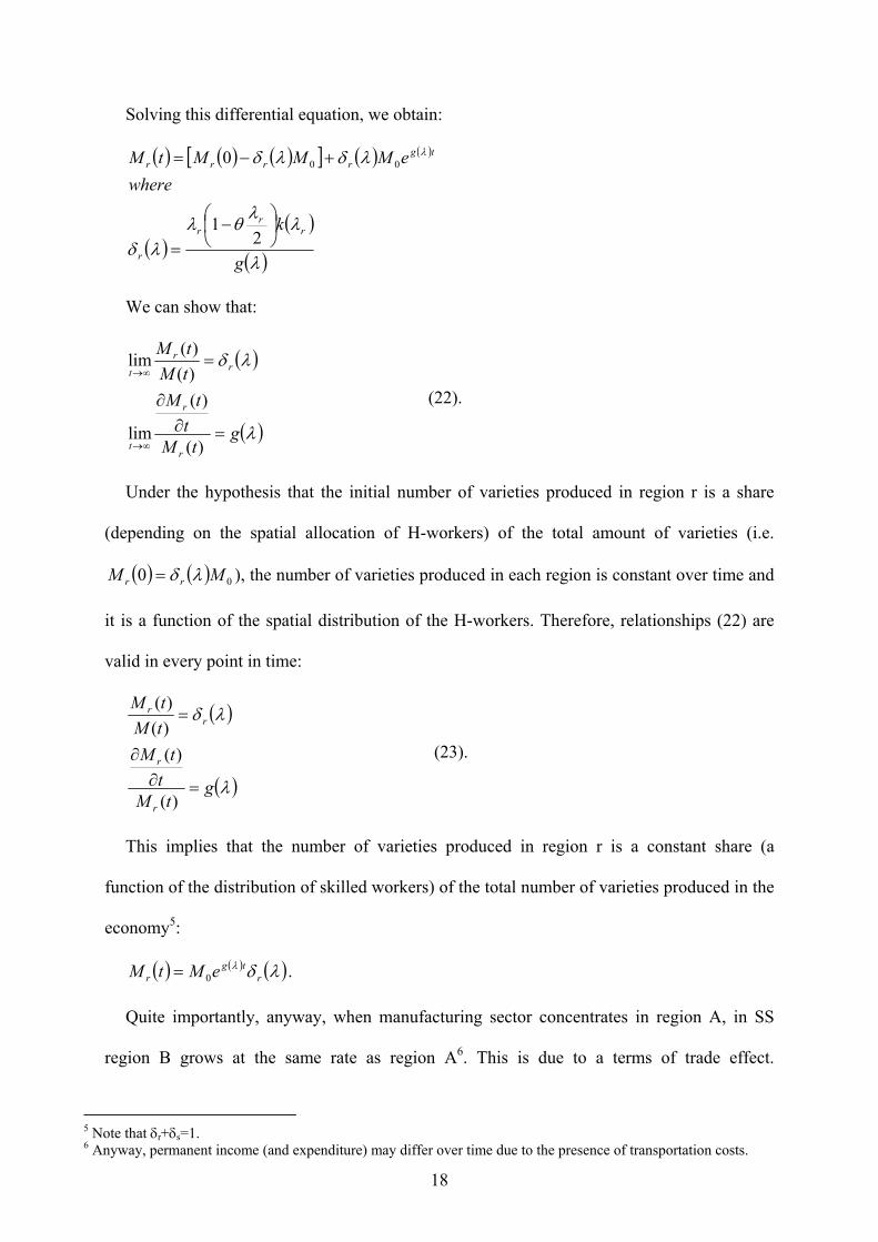
Proposition 2:

Core-periphery equilibrium maximizes the aggregate growth when CCE is small enough:

( )η

ηηθθ−

+−

−=<⇔<

78

21

231

21 gg .

−

−−∈ η

ηθ 1,

3244 .

Proof:

See Appendix 2.

Proposition 1 states that the spatial allocation of skilled workers matter for aggregate

growth. But, contrary to the previous models of “Agglomeration and Growth” (characterized

only by localised knowledge spillovers) Agglomeration does not necessarily foster growth

because of the presence of the CCE. In particular, when commuting costs are low (case a),

KSE is stronger than CCE and aggregate growth is maximised only when agglomeration

occurs4. When commuting costs are large (case b), CCE is larger than KSE and growth is

maximized when skilled workers are perfectly split between the two regions. For intermediate

levels of commuting costs (case c), both symmetric and agglomerated equilibria represent

local maxima. Proposition 2 is able to detect whether, in case c, aggregate growth is lower

under symmetry than under agglomeration. In particular, for commuting costs smaller than θ ,

core-periphery maximises aggregate growth because KSE is larger than CCE.

3.4 Market Clearing We can now determine the Market clearing conditions for unskilled and skilled workers.

4 This result is similar to Fujita-Thisse (2002).

15

*rr

Mr qML = is the demand of unskilled workers by the M-sector in region r and:

( ) BABAMB

MA EEEEEELL +≡

−=+

−=+ ,11

σσµ

σσµ

where E is the aggregate expenditure in the economy.

Demand for unskilled workers by the T-sector in the economy is . Market

clearing condition for unskilled workers implies and, in equilibrium,

aggregate expenditure:

( )ELT µ−= 1

LLLL MB

MA

T 2=++

σµ

−=

1

2LE (18).

Eq.(18) shows that aggregate expenditure is constant over time and it solely depends on the

total number of unskilled, on the share of manufacturing on expenditure and on the

monopolistic distortion in the M-sector. Moreover, eq. (18) implies that expenditure path is

constant over time and consumers smooth their consumption. Therefore, eq. (7) is equal to

zero and υ(t) = γ in each point in time. Instantaneous individual expenditure equals a share γ

of the present discounted value of individual incomes. Finally, we can state the incomplete

specialisation condition in a more formal way: the T-sector is active in both regions if

production of T-good in one region is not sufficient to cover the whole economy demand, i.e.

L<(1-µ)2L/(1-µ/σ) ⇒ µ< σ/(2σ -1).

Skilled workers market clearing conditions are obtained by imposing the zero profit

condition to the industrial sector. With perfect capital markets, entrepreneurs invest the

present discounted value of the operating profits to buy one patent to start the production.

The average cost for producing one patent is given by the ratio between the H-worker

wage and the production function of one patent

−+

−

21

21 s

sr

r

r

M

wλ

θηλλ

θλ.

16

For the zero-profit condition, the cost of one patent must equalize the present discounted

value of the operating profits, Π . Equilibrium wage for the H-workers is therefore: r

( )

( )

−+

−≡

Π=

21

21

*

ss

rrr

rrr

k

Mkw

λθηλ

λθλλ

λ (19).

3.5 Migration dynamics Skilled workers migration decisions are linked to the possible rise of real expenditure

differential between the two regions. In this paper we just assume, like in Krugman (1991), a

very simple law of motion for the skilled workers.

Each H-worker migrates to the region where her lifetime utility level is higher than the

national average:

( )

( )

( )( BA

BA

A

VVt

VVV

where

VVt

−−=∂∂

⇒

−+=

−=∂∂

λψλλλλ

ψλ

)

λ

1

1 (20).

Where ψ >0 is the speed of adjustment. This first order differential equation is in

equilibrium when λ =0, 1 or when VA=VB.

4. Agglomeration and Growth with immobile patents

4.1 SS-growth path when λ is fixed Suppose that each patent created in region r can be used only by manufacturing firms in

region r, that is patents are not transferable. The number of new varieties in each region is

equal to:

( ) ( ) ( )tgr

rrr

rr

r eMkMkt

M λλλ

θλλλ

θλ 021

21

−=

−=

∂∂ (21).

17

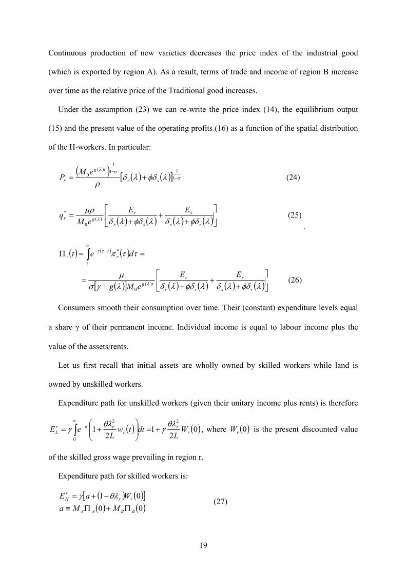
Solving this differential equation, we obtain:

( ) ( ) ( )[ ] ( ) ( )

( )( )

( )λ

λλ

θλλδ

λδλδ λ

g

k

whereeMMMtM

rr

r

r

tgrrrr

−

=

+−=

21

0 00

We can show that:

( )

( )λ

λδ

gtM

ttM

tMtM

r

r

t

rr

t

=∂∂

=

∞→

∞→

)(

)(

lim

)()(

lim

(22).

Under the hypothesis that the initial number of varieties produced in region r is a share

(depending on the spatial allocation of H-workers) of the total amount of varieties (i.e.

( ) ( ) 00 MM rr λδ= ), the number of varieties produced in each region is constant over time and

it is a function of the spatial distribution of the H-workers. Therefore, relationships (22) are

valid in every point in time:

( )

( )λ

λδ

gtM

ttM

tMtM

r

r

rr

=∂∂

=

)(

)()()(

(23).

This implies that the number of varieties produced in region r is a constant share (a

function of the distribution of skilled workers) of the total number of varieties produced in the

economy5:

( ) ( ) ( )λδλr

tgr eMtM 0= .

Quite importantly, anyway, when manufacturing sector concentrates in region A, in SS

region B grows at the same rate as region A6. This is due to a terms of trade effect.

5 Note that δr+δs=1. 6 Anyway, permanent income (and expenditure) may differ over time due to the presence of transportation costs.

18

Continuous production of new varieties decreases the price index of the industrial good

(which is exported by region A). As a result, terms of trade and income of region B increase

over time as the relative price of the Traditional good increases.

Under the assumption (23) we can re-write the price index (14), the equilibrium output

(15) and the present value of the operating profits (16) as a function of the spatial distribution

of the H-workers. In particular:

( ) ( ) ( )[ ]

( ) ( ) ( ) ( )

( ) ( ) ( )

( )[ ] ( ) ( ) ( ) ( ) (26)

(25)

(24)

)(0

*r

)(0

*

111

1)(

0

+

+++

=

==Π

+

++

=

+=

∫∞

−−

−−

λφδλδλφδλδλγσµ

ττπ

λφδλδλφδλδµρ

λφδλδρ

λ

τγ

λ

σσλ

rs

s

sr

rtg

tr

t

rs

s

sr

rgr

sr

tg

r

EEeMg

det

EEeM

q

eMP

.

Consumers smooth their consumption over time. Their (constant) expenditure levels equal

a share γ of their permanent income. Individual income is equal to labour income plus the

value of the assets/rents.

Let us first recall that initial assets are wholly owned by skilled workers while land is

owned by unskilled workers.

Expenditure path for unskilled workers (given their unitary income plus rents) is therefore

( ) ( )02

12

12

0

2

rr

rrtr

L WL

dttwL

eEθλ

γθλ

γ γ +=

+= ∫

∞− , where ( )0rW is the present discounted value

of the skilled gross wage prevailing in region r.

Expenditure path for skilled workers is:

( ) ([ ]( ) ( )00

01

BBAA

rrrH

MMaWaEΠ+Π≡

−+= θλγ ) (27)

19

where is the value of all M-firms at time zero (initial value of the assets). Regional

expenditure is therefore:

a

( )

−++=+= 0

21 rrr

rHr

rLr WaLELEE λθγλλ (28).

Using (23), (26) and (27) we obtain:

( )[ ]λγσµ

gEa+

= (29)

From equation (19), we obtain:

( ) ( )[ ]

+

+++

=)()()()()(

0λφδλδ

φλφδλδλγγσ

λµ

rs

s

sr

rrr

EEg

kW (30).

Substituting (29) and (30) in (28), we obtain a system of two equations in two unknown:

( )[ ] ( ) ( ) ( ) ( ) ( )BA,r

21

=

+

++

−+

++=

λφδλδφ

λφδλδλλθγ

λγσµλ

rs

s

sr

rrr

rr

EEkE

gLE

(31)

Which describes the equilibrium level of expenditure for each region, EA*(λ ) and EB

*(λ ),

as a function of the distribution of skilled workers between region A and B.

Substituting EA*(λ ) and EB

*(λ ) in (19) and (26), we obtain the present wage rate for

region r for every spatial distribution of H-workers.

4.2 SS-growth path when migration is allowed Like in Fujita and Thisse (2002), in order to find a migration-proof SS-growth path, we

must consider every possible migration path for the skilled workers. H-workers, indeed, are

allowed to migrate every time their life-time utility level is higher in one region than in

20

another. A migration proof equilibrium is a spatial equilibrium in which each worker does not

have any incentive to “change place” over time7.

Consider, for each t>0, a piecewise continuous function ϕ(t) which assumes the value one

when the individual is located in A and zero when she is located in B.

Be ( )( ⋅ϕλ, )~W the present discounted value of all the net wages received by a skilled

worker according to her migration path.

( )( ) ( )( ) ( ) ( )[ ] ( )[ ] ( )

( ) ( ) ( ) ( )[ ] ( )

( )∫

∫∫

∞−

∞−

∞−

≡

−−−+−=

=−−−+−=⋅

0

**0

*

0

*

1111

1111,~

dtte

ww

dtwtedtwteW

t

BA

Bt

At

ϕγϕ

λλθϕλθλϕ

λλθϕλθλϕϕλ

γ

γγ

(32)

Where ϕ is the (present discounted) share of time spent in region A.

We can define V(λ,ϕ(⋅)) the life-time utility of a skilled worker when she chooses a

location path ϕ(⋅). Using (5), (10) and (32), lifetime utility can be expressed as:

( ) ( ) ( )[ ] ( ) ( ) ( )[ ] ( ){ }

( ) [ ] ( ) ( )[ ] ( )[ ] ( ) ( )∫

∫∞

−

∞−

−

−−−−+−+=

=−+−++=

0

**

0

lnln11)1(1ln1

ln1ln,~ln1ln1,

dttPePwwa

dttPttPteWaV

Bt

BABA

BAt

H

γ

γ

µλϕγµλλθϕλθλϕλγ

γ

ϕϕµϕλλγ

γγ

ϕλ

(33)

where ( ) ( )( )tPtPP

B

A

BA ≡λ . A skilled worker chooses an optimal location path by maximising

eq. (33) for ϕ .

First and second order conditions for eq.(33) are:

( ) [ ] ( ) ( )[ ] ( )( ) [ ] ( ) ( ) ( )[ ] ( )

( )γ

λµ

λλθϕλθλϕλγλλθλθλ

γϕϕλ B

A

BA

BAHP

wwawwV ln

11111111,

**

**

−−−−+−+

−−−−=

∂∂ (34)

7 This interpretation of the SS spatial distribution of skilled workers is quite narrow. In a SS equilibrium with forward looking migration, a skilled worker can optimize her lifetime utility level with seasonal migration. This leads to a quite challenging mathematical representation of a SS equilibrium, therefore we leave this extension to further contributions.

21

( ) ( )[ ] ( ) ( )[ ]{ }( ) ( )[ ] ( ) ( ) ( )[ ] ( ){ } 0

1111

1111,2**

2**

2

2

≤−−−+−+

−−−−−=

∂

∂

λλθϕλθλϕλγ

λθλθλλγϕ

ϕλ

BA

BAH

wwa

wwV (35).

Proposition 3:

If a SS-growth path is not a Core-Periphery configuration, then it is a symmetric

equilibrium.

Proof:

See Appendix 2.

Proposition 3 implies that when Core-Periphery configuration is unstable, symmetry

prevails. We now turn to analyse the stability of the Core-Periphery solution.

In particular λ=1 is stable, i.e. V maximises the lifetime utility level for an H-worker, if

and only if:

( )1,1

( )0

,1

1

≥∂∂

=ϕ

ϕϕHV

that is:

[ ] ( ) ( )( ) [ ] ( ) ( )1ln

1111111

*

**

BA

A

BA Pwaww

γµ

θγθ

γ≥

−+−− (36).

Using wage, price and growth equations and reminding that

( ) ( ) ( ) LEEELELE BAB

σµσµ

σµ

−

+=−==

−=

1

111 ,1 ,

1

2 we obtain that:

22

( )

( )( )

( ) 11

22

2

2

1

11

14

1

21

1

1

2

41

21

1

−=

−−+

−

+−+

−

=

−

+−+

−

=

σφ

φ

φσµφ

σµθθγσ

θµη

σµθθγσ

θµ

BA

B

A

P

Lw

Lw

.

Substituting in (36):

( )( )

( ) ( ) φσµφ

σµφ

φηθ

θθγ

θ

φ ln1

1112

211

21

22

−−

−−+−−

−−+

−=Γ (37).

When ( )φΓ ≥0, core-periphery structure is sustainable, while, when ( )φΓ <0 the only stable

equilibrium is the symmetric one.

Contrary to the previous models of “Agglomeration and Growth”, when trade costs are

zero (φ is equal to one) the core-periphery structure is sustainable under a very special

assumption on knowledge spillovers or commuting costs. In particular,

( )

−≤

−≤⇔≥Γ

(38b) 1

(38a) 101

ηθ

θηor .

Conditions (38a) and (38b) state that CP structure emerges when trade costs are zero if

knowledge spillovers (commuting costs) are low enough compared to the commuting costs

(knowledge spillovers). Therefore, when free trade prevails, CP structure emerges if dynamic

centripetal (centrifugal) force is strong (weak). Comparing condition (38b) to Proposition 1

(case b), we notice that CP is still sustainable under free trade only if the aggregate growth

function is not concave, i.e. CP configuration is at least a local maximum.

23

( )φΓ

( )0 =

is a concave function, with a unique maximum in φ*. Moreover,

. We can obtain three different configurations (or outcomes): ( ) 01', <Γ−∞Γ

(a) ( ) ( )ηθθη −≤−≤ 1or 1 , ( ) 0: =Γ∃ sustainsustain φφ ;

(b) ( ) ( ) ( ) ( ) [ ]2121* ,,0:, ,0,1or 1 SSSS φφφφφφφηθθη ∈∀≥Γ∃>Γ−>−> ;

(c) ( ) ( ) ( ) [ ]1,0,0 ,1or 1 ∈∀<Γ−>−> φφηθθη .

In case (a), Core-Periphery structure of the economy is sustainable only for low values of

trade costs. In particular, for a level of φ between zero and φsustain symmetry prevails and no

divergence occurs, while, for a level of φ between φsustain and one, peripheral region

permanently looses all its industrial activities and CP and income divergence occur.

In case (b), Core-Periphery is sustainable only for an intermediate range of trade costs. In

particular, for a level of φ between zero and φs1 and between φs2 and one symmetry prevails,

while for a level between φs1 and φs2, peripheral region experiences a temporary loss of the

industrial activities (and income divergence occurs). Indeed, only for [ ]21 , ss φφφ ∈ , the

advantage of a lower price index (Centripetal force) in the core is bigger than the

disadvantage of lower net wage (centrifugal force).

In case (c), Core-Periphery is never sustainable. Commuting costs or Knowledge

Spillovers are too high and H-workers tend to be dispersed over space.

Figure 1 shows a graphical representation of Configurations (a), (b) and (c) achieved with

a numerical simulation8. We assume the following values of parameters: σ = 2.5; γ = 0.02; θ =

0.3; µ = 0.6 and we evaluate function ( )φΓ for three values of η=0.6, 0.73 and 0.85.

As figure 1 shows, as knowledge spillovers increase, ( )φΓ shifts downward.

For a low value of knowledge spillovers, Configuration (a) prevails (blue, continuous line).

For an intermediate value of knowledge spillovers, Configuration (b) prevails (green,

dashed line). 8 Unfortunately, we are not able to analytically distinguish Configuration (b) from Configuration (c).

24

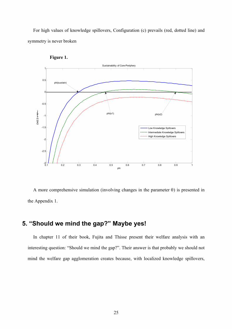
For high values of knowledge spillovers, Configuration (c) prevails (red, dotted line) and

symmetry is never broken

Figure 1.

0.1 0.2 0.3 0.4 0.5 0.6 0.7 0.8 0.9 1-3

-2.5

-2

-1.5

-1

-0.5

0

0.5

1

phi

Gamma(phi)

Sustainability of Core-Periphery

Low Knowledge Spillovers

Intermediate Knowledge Spillovers

High Knowledge Spillovers

phi(sustain)

phi(s1) phi(s2)

A more comprehensive simulation (involving changes in the parameter θ) is presented in

the Appendix 1.

5. “Should we mind the gap?” Maybe yes!

In chapter 11 of their book, Fujita and Thisse present their welfare analysis with an

interesting question: “Should we mind the gap?”. Their answer is that probably we should not

mind the welfare gap agglomeration creates because, with localized knowledge spillovers,

25

static loss of unskilled workers in the periphery (i.e. higher price level) can be overcome by

dynamic gains due to higher growth9.

In this model, anyway, we allowed for the existence of congestion costs adding both an

additional static loss (i.e. loss of housing rents) and an additional dynamic loss (lower growth

due to commuting) for the unskilled living in the periphery. Therefore, our answer to the

question “should we mind the gap?” is less optimistic than Fujita and Thisse and we can

conclude that probably we should really mind the gap.

Our welfare analysis will focus on the unskilled workers living in the periphery. It is easy

to show that skilled workers always choose their migration pattern to maximise the present

discounted value of the utility levels. Therefore, agglomeration never occurs if it does not

maximise their welfare. Unskilled workers living in the core are always better-off than the

unskilled in the periphery. Therefore, Pareto optimality of agglomeration emerges if unskilled

workers are at least indifferent (or better-off) under agglomeration compared to dispersion.

Core-periphery configuration implies, for an unskilled living in the periphery, on one side

a higher price level and the loss of the housing rents (static loss), on the other side a possible

gain in terms of higher rate of aggregate growth (dynamic gain).

In a more formal way, expenditure, at each point in time for an L-worker residing in B

composed by her labour income plus the Aggregate Land Rent per capita:

( ) ( )( )L

wtE BBL 2

11,2* λλθ

λ−

+= (39)

Substituting (39) and (24) in (11) and recalling that Traditional good is our nummeraire,

we obtain:

9 Fujita and Thisse conclude that “the increase of regional disparities does not necessarily imply the impoverishment of the peripheral region. […] it is not clear that agglomeration, growth and equity do conflict: even people residing in the periphery are better-off in core-periphery structure than under dispersion”

26

( )( )( )

( )( ) ( ) ( )[ ]µ

σσλ

λφδλδρ

λλθ

λ

+

−+

=

−−

111

1

0

2*

212

,

BA

tg

B

BL

eM

LwL

tV (40).

Which is the utility level for an L-worker residing in region B at time t under a distribution

λ of H-workers. The ratio between the utility level under Core-Periphery over the utility level

under symmetry is:

( )( )

( )

−

−

+

+

=

−

tggwL

L

tV

tV

BB

L

BL

211

1exp

121

21

42

2

21,

1,1

* σµ

φ

φθ

σµ

(41).

Recalling, from (5), that:

( ) ( )∫∞

−

=

−

0

21,

1,ln

211 dt

tV

tVeVV

BL

BLtB

LB

Lγ (42)

we obtain:

( ) ( )

−

−+

+−+

+

=

−

211

11

12ln

121

42

2ln1211 2

*gg

wL

LVB

BL

BL σ

µγφ

φσµ

θγV (43).

Equation (43) describes the welfare gain/loss for an unskilled in B when a core-periphery

configuration emerges. The term in squared brackets, on the right hand side of the equation,

describes the static loss derived by agglomeration. In particular,

+

21

42

2*BwL

Lθ

ln <0 is the

housing rent loss occurring when skilled workers leave region B for region A.

φφ

σµ

+− 12ln

1<0 is the price level loss when unskilled workers in B have to pay a higher price

(due to transport costs) for all the M-good varieties (while they had to pay transport costs only

27

on half of the varieties under symmetry). ( )

−

− 211

1gg

σµ is the (possible) dynamic gain

from agglomeration derived by higher growth under core-periphery. A necessary condition to

have an overall welfare improvement is that growth under core-periphery should be larger

than growth under symmetry, i.e. condition stated in Proposition 2 is respected. This

condition, anyway, is not sufficient as growth acceleration should be large enough to

overcome the static losses.

From a qualitative point of view, our result is not different from Fujita and Thisse welfare

analysis: Core-periphery is Pareto improving if and only if it creates enough growth. From

quantitative point of view, instead, a huge difference emerges between the two models. On

one side, we have a much larger static loss (due to the loss of housing rents), on the other side,

we have a smaller dynamic gain as commuting costs lower the speed of creation of new

patents. As a result, we may conclude that, allowing for the presence of commuting costs,

eq.(43) is less likely to be bigger than zero than the equivalent condition in Fujita and Thisse

(2002).

6. Conclusions

In this model we showed the effects of commuting costs on the process of Agglomeration

and Growth. Contrary to the previous models of “Agglomeration and Growth”, we allowed

for the existence of an internal structure of the region and for the presence of centrifugal

forces in the form commuting costs.

Four different forces shape the spatial distribution of economic activities and the regional

income levels. (i) Static centripetal forces are due to economies of scale and transport costs.

(ii) Dynamic centripetal forces take the form of localized knowledge spillovers. (iii) Static

centrifugal forces are linked to market-crowding and commuting costs (lowering net wages).

(iv) Dynamic centrifugal forces are linked to commuting costs (slowing economic growth).

28

The interplay among these four forces creates three possible configurations of the steady

states.

Configuration (a): When knowledge spillovers (commuting costs) are particularly low,

Core-Periphery always emerges and remains stable when trade costs lowers. As a result,

income levels divergence occurs and income inequality persists in the Steady State.

Configuration (b): At an intermediate value of knowledge spillovers (commuting costs),

Core-Periphery and Income divergence occur only at an intermediate level of trade costs,

while when trade costs are either too high or too low Spatial Dispersion emerges. The

economy has three phases of Convergence-Divergence-Convergence.

Configuration (c): When knowledge spillovers (commuting costs) are high, spatial

dispersion is the only outcome and income levels never diverge.

Welfare analysis shows that Core-Periphery creates a welfare gap between L-workers in

the Core and L-workers in the periphery. As a result, agglomeration creates inequality among

regions, but, nonetheless, it can be welfare improving when dynamic effects of agglomeration

are larger than static losses.

References Baldwin (1999): “Agglomeration and Endogenous capital”, European Economic Review, 43

pp. 253-280;

Baldwin and Forslid (2000): “The core-periphery model and endogenous growth: stabilizing

and de-stabilizing integration”, Economica (67);

Baldwin and Martin (2004): “Agglomeration and Regional Growth” in Henderson and Thisse:

Handbook of Regional and Urban Economics, Vol. 4, Elsevier;

Baldwin, Martin and Ottaviano (2001): “Global Income Divergence, Trade and

Industrialization: The Geography of Growth Take-Off”, Journal of Economic Growth (6) p.5-37;

29

Baldwin, Forslid, Martin, Ottaviano and Robert-Nicoud (2003): “Economic Geography and

Public Policy”, Princeton University Press, Princeton;

Basevi and Ottaviano (2003): “The district goes global: Export vs. FDI”, Journal of Regional

Science (42) p.107-126;

Cerina and Pigliaru: “Agglomeration and Growth in the NEG: a critical assessment”, w.p.

2005/10, CRENOS;

Combes and Overman (2004): “The spatial distribution of economic activities in the European

Union” in Henderson and Thisse: Handbook of Regional and Urban Economics, Vol. 4, Elsevier;

Fujita and Thisse (2002): “Economics of Agglomeration: cities industrial location and regional

growth”, Cambridge University Press;

Grossman and Helpman (1991): “Innovation and Growth in the Global Economy”, MIT press;

Hohenberg and Lees (1985): “The Making of Urban Europe (1000-1950)”, Harvard University

Press;

Holmes and Stevens (2004): “Spatial Distribution of Economic Activities in North America” in

Henderson and Thisse: Handbook of Regional and Urban Economics, Vol. 4, Elsevier;

Krugman (1991): “Increasing Returns and Economic Geography”, Journal of Political

Economy (99:3);

Martin and Ottaviano (1999): “Growing locations: industry location in a model of endogenous

growth”, European Economic Review 43: 281-302;

Martin and Ottaviano (2001): “Agglomeration and Growth”, International Economic Review;

Murata and Thisse (2005): “A simple model of economic geography à la Helpman-Tabuchi”,

Journal of Urban Economics (58);

Romer (1990): “Endogenous Technical Change”, Journal of Political Economy (5:2);

Urban: “Neoclassical growth, manufacturing agglomeration and terms of trade”, mimeo LSE;

Walz (1996): “Transport costs, intermediate goods and localized growth”, Regional Science

and Urban Economics, 26 pp. 671-695;

30

Walz (1997): “Growth and deeper regional integration in a three-country model”, Review of

International Economics, 5 pp. 492-507.

Appendix 1: Simulations and Comparative Statics

The values of the sustain points φsustain, φs1 and φs2 may vary at any change of knowledge

spillovers and commuting costs.

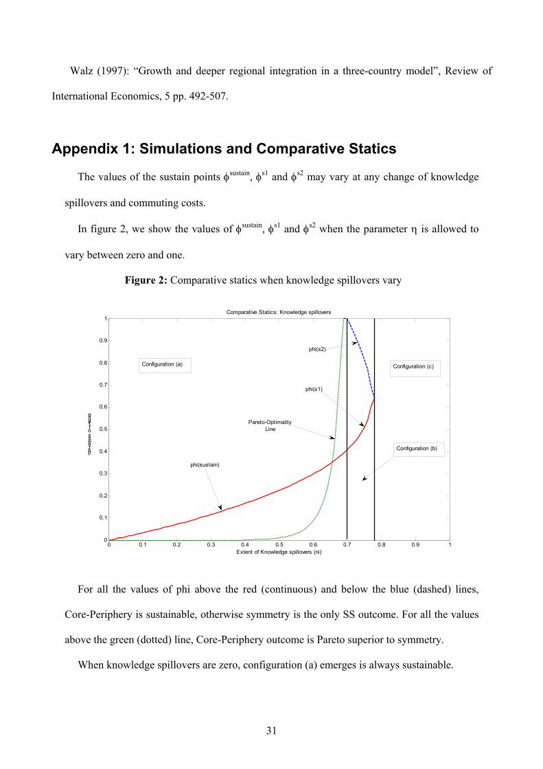
In figure 2, we show the values of φsustain, φs1 and φs2 when the parameter η is allowed to

vary between zero and one.

Figure 2: Comparative statics when knowledge spillovers vary

0 0.1 0.2 0.3 0.4 0.5 0.6 0.7 0.8 0.9 10

0.1

0.2

0.3

0.4

0.5

0.6

0.7

0.8

0.9

1Comparative Statics: Knowledge spillovers

Extent of Knowledge spillovers (ni)

phi-ness of trade

Pareto-OptimalityLine

phi(sustain)

phi(s2)

phi(s1)

Configuration (a) Configuration (c)

Configuration (b)

For all the values of phi above the red (continuous) and below the blue (dashed) lines,

Core-Periphery is sustainable, otherwise symmetry is the only SS outcome. For all the values

above the green (dotted) line, Core-Periphery outcome is Pareto superior to symmetry.

When knowledge spillovers are zero, configuration (a) emerges is always sustainable.

31

As knowledge spillovers increase, the economy, starting from a Configuration (a) situation

changes first in a Configuration (b) and then in a Configuration (c) outcome. This is due to the

fact that dynamic centripetal forces loose their strength, and static and dynamic centrifugal

forces overcome them. It is important to notice that Core-Periphery outcome is always a

private optimum and it does not necessarily imply that all the workers are better off. Indeed,

figure 2 shows that all the CP configurations below the green (dotted) are not Pareto optimal.

A welfare maximising policy maker, therefore, should intervene to correct these externalities.

In figure 3, we show the values of φsustain, φs1 and φs2 when the parameter θ is allowed to

vary between zero and one. The picture is quite similar to the previous one.

Figure 3: Comparative Statics when Commuting Costs vary

0 0.1 0.2 0.3 0.4 0.5 0.6 0.7 0.8 0.9 10

0.1

0.2

0.3

0.4

0.5

0.6

0.7

0.8

0.9

1

Degree of Commuting costs (theta)

phi-ness of trade

Comparative Statics: Commuting Costs

phi(sustain)

phi(s1)

phi(s2)

Pareto-optimalityLine

Configuration (a) Configuration (c)

Configuration (b)

When Commuting costs are zero, there exists a unique sustain point at a high level of trade

costs. This is configuration (a) and it is equal to Fujita-Thisse (2002). When Commuting

Costs rise, the economy has the following path: Configuration (a) – Configuration (b) –

32

Configuration (c). The economic interpretation is quite straightforward. As Commuting costs

increase both dynamic and static centrifugal forces strengthen and a symmetric outcome

becomes stable, compared to the Core-Periphery configuration. As before, even in this case,

there is room for policy interventions as CP occurrence may lower the economic welfare of

the unskilled in the periphery.

Appendix 2: proofs Proof of Proposition 1:

a) Given its symmetric shape around λ=1/2, g(λ) is a strictly convex function when its

first derivative in λ=0 is negative and its second derivative in λ=1/2 is positive (in

this case the other two stationary points are either complex or outside the interval [0,

1]).

( ) ( )( ) ( )( ) ( ) ( )( )[ ]

( ) ( ) ( ) ( ) ( )( )[ ]( )

ηθ

ηθ

λληηθηθηλλ

λληηλθληθηλλ

−−≤⇔≥

−≤⇔≤

−+−++−−−−=

−+−++−+−−−−−−=

32440

21''

100'

121212344

3214''

46123444

1231212'

22

322

g

g

g

g

but ηη

−≤−

− 13

244 , ( )η

θλ−

−≤⇔3

244convex is g⇒ ;

b) Analogously, g(λ) is concave if its second derivative around λ=1/2 is positive as it is

shown in point (a);

c) For

−

−− η

η1,

3244∈θ , g(λ) is decreasing (increasing) in λ=0 (1), and λ=1/2 is

a local maximum. This implies that there exists two additional stationary points

(symmetric around λ=1/2, local minima).

33

Proof of Proposition 2:

( )

( ) ( ) ( ) ( )

( )η

ηηθ

ηηθηθη

θθ

−

+−

−≤⇔

≥⇒

+−++−+

−−−−−=

+−=

78

21

23

211

1833

2121

43

4111

211

21

411

2

2

gg

g

g

Proof of Proposition 3:

ϕ

0∈

takes the value of one, when the H-worker spend all her life in region A, while it takes

the value of zero, when she spends all her life in region B. Therefore, spatial distribution

( 1, )λ is migration-proof if and only if the present discounted utility level in region A is

equal to the present discounted utility level in region B. This means that V(λ, 1) = V(λ, 0) =

max { ( )ϕλ,V :ϕ ∈[0, 1]}. This implies that ( )ϕλ,V is not strictly concave on the compact set

[ ]1,0∈ϕ . Hence, in order to ( )1,0∈λ be as a maximum (and eq. 35 to hold),

. Therefore eq. 34 is equal to zero (and ( ) ([ λθ −−= 11*Bw )] )θλ−1*

Aw ( 1,0∈λ is a maximum)

if and only if ( )λB

AP =1. This happens when λ=1/2.

34