agglomeration effects on labor productivity: an … · 1 agglomeration effects on labor...
TRANSCRIPT

Agglomeration effects on labor
productivity: An assessment with
microdata
Stephan Brunow and Uwe Blien
NORFACE MIGRATION Discussion Paper No. 2014-06
www.norface-migration.org

1
Agglomeration effects on labor productivity: An assessment
with microdata
Stephan Brunow1, Uwe Blien2,
Institute for Employment Research (IAB) and Otto-Friedrich-University of Bamberg
Abstract
Urbanization and localization effects are known to boost the regional economy and its growth
potential. The emergence of these effects is due to localized knowledge flows, the closeness
to markets, but also due to the diversity of services and industries. All these effects have the
potential to increase the productivity (and profitability) of firms. Whereas many studies have
been conducted at the industry or the regional level, this paper adds to the existing literature
by starting at the level of establishments and taking the interaction with the surrounding
regions into account. This is possible by exploiting an exceptionally large establishment
panel study and the employment statistics for Germany. The empirical analyses are carried
out in two steps regressions in order to separate the characteristics of establishments from
regional influences.
Keywords: Region, labor productivity, agglomeration effects, MAR-, Jacobs-effects
Acknowledgement: The research is part of the NORFACE research programme on migration
(Migrant Diversity and Regional Disparity in Europe – MIDI-REDIE project). The authors gratefully
acknowledge the many ideas and comments they have received in this context at the ERSA, GfR and
NARSC conferences, at the AQR-Workshop 2013 in Barcelona, from the team colleagues Thomas de
Graaf, Peter Nijkamp, Jacques Poot, and many others.
The responsibility for the analysis and the results remains completely with the authors.
1 [email protected] (corresponding author); +49-(0)911-179 65 26; Regensburger Str. 104; 90478 Nuremberg/ Germany
2
1. Introduction
Urbanization and localization effects have the potential to boost the regional economy and its
growth (Rosenthal/Strange 2004). The emergence of these effects is due to localized
knowledge flows (Glaeser et al. 2011), the closeness to markets (Krugman 1991) but also
due to the diversity of services and industries (Jacobs 1969).
The paper concentrates on the effects of agglomeration on labor productivity of firms, since
the dynamics of an economy are strongly influenced by this crucial variable. According to
common beliefs the metropolitan areas are the regions which are decisive for an economy.
They are the places where innovations happen and from where these innovations spread out
over the country and even over the world. Since Marshall (1920), in economic theory
arguments have been collected which relate agglomeration effects to the performance of
firms. We intend to have a closer look at the empirics of productivity in order to relate
regional differences to agglomeration effects.
Though many studies have been conducted concerning agglomeration effects, thorough
analyses with microdata are still rare, especially from the perspective of individual firms. This
paper contributes to filling this gap by analyzing regional (intra-industrial) agglomeration
economies which may influence labor productivity by using microdata from an exceptionally
large establishment panel study and from the employment statistics of Germany. The
intention of the paper is to look into the interaction of productivity and the regional economy
to see whether agglomeration effects matter. The available microdata are integrated into a
linked employer-employee panel data set, which facilitates the analysis carried out in several
steps.
The task intended is difficult, because standard methods of panel analysis are not
appropriate, since agglomeration forces vary rather slowly. Therefore, though we have a
‘long panel‘, variations of standard approaches have to be used to identify and measure
agglomeration effects. The approach chosen has the advantage that effects at various levels
can be studied. The interaction of establishments, industries and regions is taken into
account. This requires a detailed measurement of the performance and of the mechanics of
establishments or plants. It is necessary to control for many variables at this level to be able
to identify the interaction with properties of the local economy. Concerning the regions we
are able to use rather small units: In Germany there are 412 districts (“Kreise”). For the
effects of larger units we use distance matrixes.
In the following we start with a brief outline of the theory and a derivation of an identification
strategy. It is inspired by the multi-step approach used by Bell, Nickell & Quintini (2002).
Then we will give an outline of the (excellent) data source we use. As usual we report the
empirical analyses before we come to a conclusion.

3
2. Theoretical considerations
In recent times the standard approach of research on agglomeration effects which used
aggregate data has been more and more replaced by efforts based on microdata. Examples
in this respect are Baldwin, Brown & Rigby (2010), Drucker & Feser (2012). Before
developing an empirical model it is necessary to clarify some major points. One of these is
that agglomeration forces affect different economic variables differently (Rosenthal &
Strange, 2004; Puga, 2010). The effects on productivity and employment might be in the
same line or they might be even contradictory as Cingano & Shivardi (2004) have shown.
Due to the labor-saving effect of productivity gains it is possible that agglomeration effects on
productivity might affect employment negatively. On the other hand, increases in productivity
typically reduce prices and this might increase employment (see also Blien & Sanner 2014,
Combes, Robin & Magnac 2004). This compensating effect on employment might even be
stronger than the labor-saving effect. Most of the literature has concentrated on employment
and wages, whereas we address productivity at the establishment level.
A discussion of causes and the magnitude of agglomeration effects and a review of earlier
literature is provided by Puga (2010). The most striking challenge is the potential bias due to
endogeneity. Most of the empirical literature focuses on aggregated data and several
potentials of a bias in estimates are discussed. However, there already exists a well-
documented literature, as cited by Puga (2010), showing that the bias is a minor point.
Henderson’s (2003) contribution rests on plant level data. He provides evidence for high-tech
and machinery plants located in the US of the effect of agglomeration forces on the output of
plants. He finds strong support for a positive influence of such effects on output while
carefully dealing with potential biases due to endogeneity.
Other literature on the micro level uses individual employment data. In a first step regression,
individual wages are explained by a Mincerian wage equation and some region-time-fixed
effects. These effects are then regressed in a second step using determinants of
agglomeration. Our approach is related to such a procedure but rests on establishment data
rather than individual employment data.
Often it is assumed that production can be described by a Cobb-Douglas production function.
We assume a more general functional form of an establishment’s production by specifying a
CES function (constant elasticity of substitution), given by
[ ( )
( )
]
. (1)
Total production is produced with labor and capital , where and are parameters that
describe the input shares, and and relate to labor and capital productivity, respectively.
The elasticity of substitution between labor and capital is described by . For , the
production function becomes of Cobb-Douglas-type. For a level of sales , factor prices
for wages and for the interest rate, the compensated factor demand for labor is given by:
4
(
)
(
) . (2)
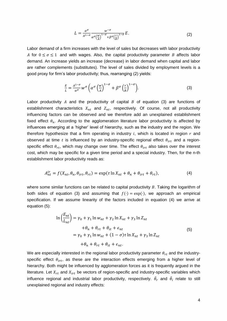
Labor demand of a firm increases with the level of sales but decreases with labor productivity
for and with wages. Also, the capital productivity parameter affects labor
demand. An increase yields an increase (decrease) in labor demand when capital and labor
are rather complements (substitutes). The level of sales divided by employment levels is a
good proxy for firm’s labor productivity; thus, rearranging (2) yields:
( (
)
(
)
). (3)
Labor productivity and the productivity of capital of equation (3) are functions of
establishment characteristics and , respectively. Of course, not all productivity
influencing factors can be observed and we therefore add an unexplained establishment
fixed effect . According to the agglomeration literature labor productivity is affected by
influences emerging at a ‘higher’ level of hierarchy, such as the industry and the region. We
therefore hypothesize that a firm operating in industry , which is located in region and
observed at time is influenced by an industry-specific regional effect and a region-
specific effect , which may change over time. The effect also takes over the interest
cost, which may be specific for a given time period and a special industry. Then, for the n-th
establishment labor productivity reads as:
( ) ( ), (4)
where some similar functions can be related to capital productivity . Taking the logarithm of
both sides of equation (3) and assuming that ( ) ( ), we approach an empirical
specification. If we assume linearity of the factors included in equation (4) we arrive at
equation (5):
( )
( )
.
(5)
We are especially interested in the regional labor productivity parameter and the industry-
specific effect , as these are the interaction effects emerging from a higher level of
hierarchy. Both might be influenced by agglomeration forces as it is frequently argued in the
literature. Let and be vectors of region-specific and industry-specific variables which
influence regional and industrial labor productivity, respectively. and relate to still
unexplained regional and industry effects:

5
(6)
with and parameters that describe the change in labor productivity at the higher level.
Eventually, we substitute equation (6) into (5) which approaches an augmented empirical
specification:
( )
(7)
Unobserved time fixed effects are captured by , whereas relates to an unexplained IID
error term. In the next section we discuss estimation issues of the models presented in
equations (5) and (7).
3. Empirical model description and identification strategy
Equation (7) can be generalized into two equations, which integrate a different number of
variables.
(8a: Model 1)
(8b: Model 2)
with . (8c)
relates to the log of sales per employee. The set of includes all variables that relate to
the nth establishment during period t. It might include time constant variables. Accordingly,
and relate to sets of variables of the industry and regional level, respectively. The
parameters are as described above and is a composite establishment specific fixed effect.
The estimation strategy is inspired by the approach of Bell, Nickell & Quintini (2002, which
was suggested in turn by Card 1995). This is a two-step approach, which starts with an
analysis at the level of individual observations (workers in the case of Bell et al.,
establishments in our case). In a second step the variation between regions (and possibly
periods) is analyzed. At the first step we control for the many influences on productivity which
are specific for individual establishments. The regional and intra-industrial average, and
, respectively, included in the establishment fixed effects is then used in the second step
to identify agglomeration effects and effects of other region specific variables. It is not
possible to integrate both steps into one, since some of the variables characterizing a region
do not vary in time and therefore drop out in a fixed effects approach. However, such a 2-
step approach is required to control for unobserved properties of establishments.
6
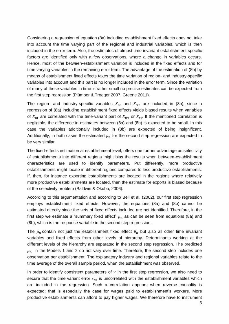
Considering a regression of equation (8a) including establishment fixed effects does not take
into account the time varying part of the regional and industrial variables, which is then
included in the error term. Also, the estimates of almost time-invariant establishment specific
factors are identified only with a few observations, where a change in variables occurs.
Hence, most of the between-establishment variation is included in the fixed effects and for
time varying variables in the remaining error term. The advantage of the estimation of (8b) by
means of establishment fixed effects takes the time variation of region- and industry-specific
variables into account and this part is no longer included in the error term. Since the variation
of many of these variables in time is rather small no precise estimates can be expected from
the first step regression (Plümper & Troeger 2007, Greene 2011).
The region- and industry-specific variables and are included in (8b), since a
regression of (8a) including establishment fixed effects yields biased results when variables
of are correlated with the time-variant part of or . If the mentioned correlation is
negligible, the difference in estimates between (8a) and (8b) is expected to be small. In this
case the variables additionally included in (8b) are expected of being insignificant.
Additionally, in both cases the estimated for the second step regression are expected to
be very similar.
The fixed-effects estimation at establishment level, offers one further advantage as selectivity
of establishments into different regions might bias the results when between-establishment
characteristics are used to identify parameters. Put differently, more productive
establishments might locate in different regions compared to less productive establishments.
If, then, for instance exporting establishments are located in the regions where relatively
more productive establishments are located, then the estimate for exports is biased because
of the selectivity problem (Baldwin & Okubo, 2006).
According to this argumentation and according to Bell et al. (2002), our first step regression
employs establishment fixed effects. However, the equations (8a) and (8b) cannot be
estimated directly since the sets of fixed effects included are not identified. Therefore, in the
first step we estimate a “summary fixed effect” as can be seen from equations (8a) and
(8b), which is the response variable in the second step regression.
The contain not just the establishment fixed effect but also all other time invariant
variables and fixed effects from other levels of hierarchy. Determinants working at the
different levels of the hierarchy are separated in the second step regression. The predicted
in the Models 1 and 2 do not vary over time. Therefore, the second step includes one
observation per establishment. The explanatory industry and regional variables relate to the
time average of the overall sample period, when the establishment was observed.
In order to identify consistent parameters of in the first step regression, we also need to
secure that the time variant error is uncorrelated with the establishment variables which
are included in the regression. Such a correlation appears when reverse causality is
expected; that is especially the case for wages paid to establishment’s workers. More
productive establishments can afford to pay higher wages. We therefore have to instrument
7
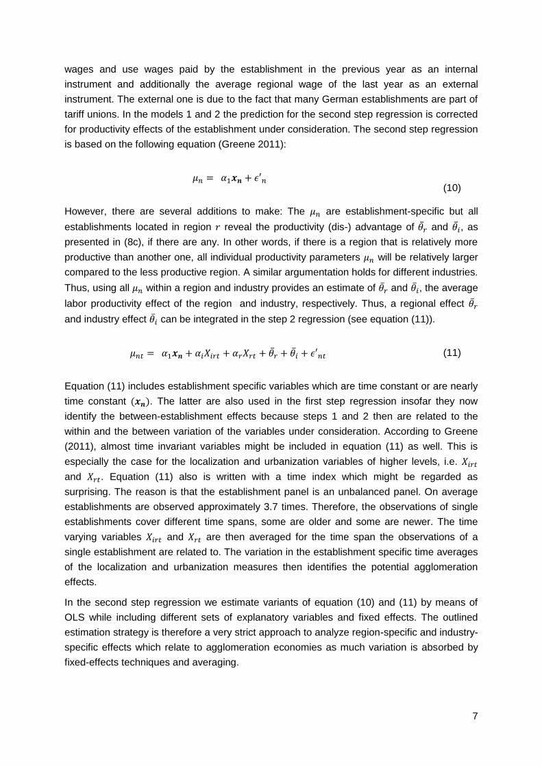
wages and use wages paid by the establishment in the previous year as an internal
instrument and additionally the average regional wage of the last year as an external
instrument. The external one is due to the fact that many German establishments are part of
tariff unions. In the models 1 and 2 the prediction for the second step regression is corrected
for productivity effects of the establishment under consideration. The second step regression
is based on the following equation (Greene 2011):
(10)
However, there are several additions to make: The are establishment-specific but all
establishments located in region reveal the productivity (dis-) advantage of and , as
presented in (8c), if there are any. In other words, if there is a region that is relatively more
productive than another one, all individual productivity parameters will be relatively larger
compared to the less productive region. A similar argumentation holds for different industries.
Thus, using all within a region and industry provides an estimate of and , the average
labor productivity effect of the region and industry, respectively. Thus, a regional effect
and industry effect can be integrated in the step 2 regression (see equation (11)).
(11)
Equation (11) includes establishment specific variables which are time constant or are nearly
time constant ( ). The latter are also used in the first step regression insofar they now
identify the between-establishment effects because steps 1 and 2 then are related to the
within and the between variation of the variables under consideration. According to Greene
(2011), almost time invariant variables might be included in equation (11) as well. This is
especially the case for the localization and urbanization variables of higher levels, i.e.
and . Equation (11) also is written with a time index which might be regarded as
surprising. The reason is that the establishment panel is an unbalanced panel. On average
establishments are observed approximately 3.7 times. Therefore, the observations of single
establishments cover different time spans, some are older and some are newer. The time
varying variables and are then averaged for the time span the observations of a
single establishment are related to. The variation in the establishment specific time averages
of the localization and urbanization measures then identifies the potential agglomeration
effects.
In the second step regression we estimate variants of equation (10) and (11) by means of
OLS while including different sets of explanatory variables and fixed effects. The outlined
estimation strategy is therefore a very strict approach to analyze region-specific and industry-
specific effects which relate to agglomeration economies as much variation is absorbed by
fixed-effects techniques and averaging.

8
4. Data
We aim to identify industry and region-time-specific labor productivity, and , which
might be influenced by regional characteristics and the economic environment. The
identification of these effects is based on the labor productivity of single establishments.
Therefore establishment or firm level data is needed. We choose Germany as research field
because for this country an excellent data basis is available, which suits our purpose: The
IAB Establishment Panel (IAB-EP) is the only representative survey of establishments for a
large economy that can uniquely be linked to other data sources. It is conducted on an
annual basis and available for a relatively long time period. From the waves of 1995 until
2010 we use vast information especially relevant for our research programme.
The establishment panel is a rotating panel which surveys 16,000 establishments annually of
which we use about 8-9,000 after some data preparation steps. In total we consider more
than 32,000 establishments during the time period. To get a consistent data set, we only
consider establishments that achieve revenues and are sole traders, partnership companies
or corporate enterprises. This restriction excludes the public sector and partly financial
institutions. We exclude about 2300 establishments which either change the reported
industry or the location on the basis of NUTS3 regions. The exclusion of relocating firms
takes care of the emerging ‘selection effect’ of firms that will overestimate agglomeration
effects as shown by Baldwin and Okubo (2006).
The second data source we use is the Employment Statistics of Germany, which include the
entire population of people gainfully employed and covered by the social insurance system in
Germany. Only self-employed, civil servants, and workers with a very small income are
excluded from this data. The Employment Statistics give continuous information on
employment spells, earnings, job and personal characteristics. It is based on microdata
delivered by firms about their individual employees. For every employee a new record is
generated every year. The same is done if he or she changes an establishment. One of the
advantages of the employment statistics is the identification of the region where a specific
employee is located.
Originally, the data of the employment statistics are taken over for administrative purposes of
the social security system and are collected by the administration of the Federal Employment
Services. Since they are used to calculate the pensions of retired people, the income and
duration information is very reliable. No wage classifications are needed because the exact
individual wage is reported. The wage variable is measured in calendar days. Apart from the
individual wage, which is averaged at the establishment level, some further variables are
used in our regressions.
In the context of our analyses, the Employment Statistics are used in a twofold way: On the
one hand an Employer-Employee database is constructed, by adding the information from
the Employment Statistics to the single establishment it is related to. This is relevant in the
case of the Human Capital variable by adding the share of highly qualified in the respective
establishments. On the other hand, the information from the Employment Statistics was

9
aggregated for the further characterization of the industries and regions under observation
that is used to identify agglomeration effects.
From the IAB-EP we take the following information. As a measure of output we use the level
of sales to construct the dependent variable, namely the output per employee. Since Melitz
(2003) argues exporting firms have to be relatively more productive to compete in foreign
markets, we use the export proportion of total sales as a proxy for international
competitiveness. Thus, such trade related productivity effects are already absorbed from the
remaining labor productivity parameter. We also use a dummy indicator that is set to unity if
the establishment is foreign owned. Foreign owners may have an interest in higher dividends
and thus, more productive companies. Empirical evidence for Spain by Benfratello and
Sembenelli (2006), however, suggests that foreign ownership does not influence productivity.
We employ two dummy indicators for the legal status, i.e. whether the firm is a sole trader or
a private partnership. The reference category therefore is given as all kinds of capital
companies. As a proxy for the productivity of capital we use information on the state of the
kind of the technology and machinery. It is an ordinal set, which includes the categories
‘newest’, ‘new’, ‘old’ and ‘out of date’ equipment. The reference category is ‘newest’
technology. As another control variable we employ two dummy indicators for the
establishment age. The first one is set to unity if the establishment is older than 4 years and
less than 15 years; and the second one relates to an establishment age equal or higher than
15 years. The reference category is therefore an age up to 4 years.
In- and outsourcing or spin-offs of companies would directly lead to a change in labor
demand as parts of the economic activities now take place within or outside of the
establishment. Therefore it is worth controlling for it: two indicators are set to unity if parts of
the establishment were insourced and outsourced, respectively. All other data of the
Employment Statistics comes from a special file of the IAB Employment History (IAB-EH)
which is fused with the establishment panel on an annual basis. It contains not just
information of the workforce employed at a reference day, but it covers the workforce
employed through the year. It takes therefore seasonal employment differences explicitly into
account. The IAB-EH provides detailed information on the occupations of the workforce on
the basis of the 2-digit occupational classification (KldB 88). We use this information and
compute diversity indices on the basis of the Fractionalization index for employees in less
complex and complex occupations (see below).
We refrain from using standard measures of ‘human capital’, such as the presence of
university degrees, for three reasons. First, there is a trend in the data that the number of
missing values of the educational attainment increases whereas the proportion of people
holding a university degree decreases over time. Second, Brunow and Hirte (2009) show that
a measure built on educational attainment is biased as it does not account for ‘over-’ and
‘under-education’; a strand of literature launched by Duncan and Hoffmann (1981). Third,
Autor et al. (2003) establish a task-based approach for jobs, which relates to the amount of
routine tasks and analytical tasks at the workplace. A task-based approach offers the
advantage that it overcomes the problem of measurement of mismatch like over-education,

10
because then, occupations are classified not just on the basis of formal qualification but also
on tasks in the job.
Our classification of human capital is inspired by Gathmann and Schönberg (2010). We use
the German Qualification and Career Survey, which was conducted jointly by the Federal
Institute for Vocational Education and Training (BIBB) and the Institute for Employment
Research (IAB) of the year 1998/1999. From this survey we relate occupations to tasks and
cluster occupations (see Spitz-Öner 2006 based on Autor et al. 2003) on the basis of, first,
the average time spent with analytical work relative to analytical and manual work. Second
we calculate non-routine work relative to routine and non-routine work. Finally we use the
proportion of human capital in the occupation on the basis of formal qualification. According
to our definition, which has also been used by Trax et al. (2012) or Brunow and Nafts (2013),
a complex occupation exhibits a relatively high proportion of time spent in non-routine and
analytical work and typically the proportion of highly qualified people is relatively large.
Following this, other occupations are then assigned into the group of ‘less complex’
occupations. For the sake of labeling, we use from now on the term ‘low-skilled’ and ‘high-
skilled’ for ‘less complex’ and ‘complex’ occupations, respectively. The classification is based
on a hierarchical cluster analysis using the average linkage method.
Because the IAB-EH covers the entire population of all employees subject to social security,
we are able to construct additional measures from this data source which are related not to
individual establishments but to industrial and regional units. First, we compute the total
number of establishments which operate in the same 2-digit industry and which are located
in the region. Second, we aggregate individual data to the regional workforce employed and
use the proportion of people working in high-skilled occupations; again measured in full-time
equivalents within the industry, to which the establishment is assigned.
For some of the variables we also use a spatially lagged version. As usual these lagged
variables are calculated by multiplication with a row-standardized, spatial weights matrix. An
element of this matrix W is computed by ( ), where relates to the
distance of the geographical centers of two regions i and j, and is a distance-decay
parameter. The parameter is set in a way that from the average neighboring region (which
has an average distance of 34 km) 70 % of the effect is present. Experiments with a variation
of this parameter show only very small differences in the regression results.
We also control for the industrial variety available in a region. The measures are suggested
e.g. by Combes et al. (2004). The number of regional established 2-digit industries aims to
control for the variety of products and services available to the establishment. We also
compute a diversity measure on the basis of the Fractionalization index that captures the
relative distribution of establishments across the industries. This measure increases the
more uniform the establishments are distributed across the industries. Both measures relate
to urbanization externalities.
From the German official statistics we use the population density of districts in Germany.
This is one of the most important variables indicating the existence of agglomerations in the
country. It is expected that the cost of population concentration, which is directly given by
11
high land prices (and high rents for flats and also of relatively high regional prices, see Blien
et al. 2009) and indirectly by the cost of congestion and of pollution, must be offset by
relatively high productivity of the establishments located there. Regional population is also a
measure of market size (see e.g. the theoretical contribution of Baldwin, 1999).
Our regional units are the mentioned districts (i.e. in German terms “Landkreise” and
“kreisfreie Städte”) which are relatively small, since there are 412 present in the country. The
smallness of the units allows a detailed picture. The disadvantage of the small-scale regional
grid is compensated by the use of the mentioned weight matrices which describe the
interdependencies of regions. Our establishment survey is sufficiently representative for
regions; we could use 411 districts in the analysis.
In addition, we use a typology of districts, which is generated by the application of two
criteria: Centrality at the level of larger regions and population density at the level of districts.
This typology has been developed and regularly updated by the German Institute BBSR (see
Görmar, Irmen 1991 and later versions from the home page of BBSR). Definitions of this
typology can be seen from Table 3.
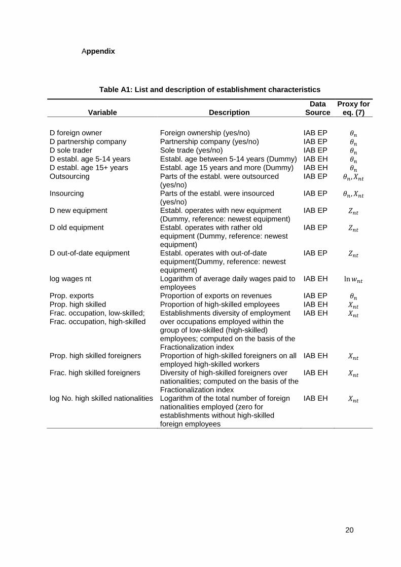
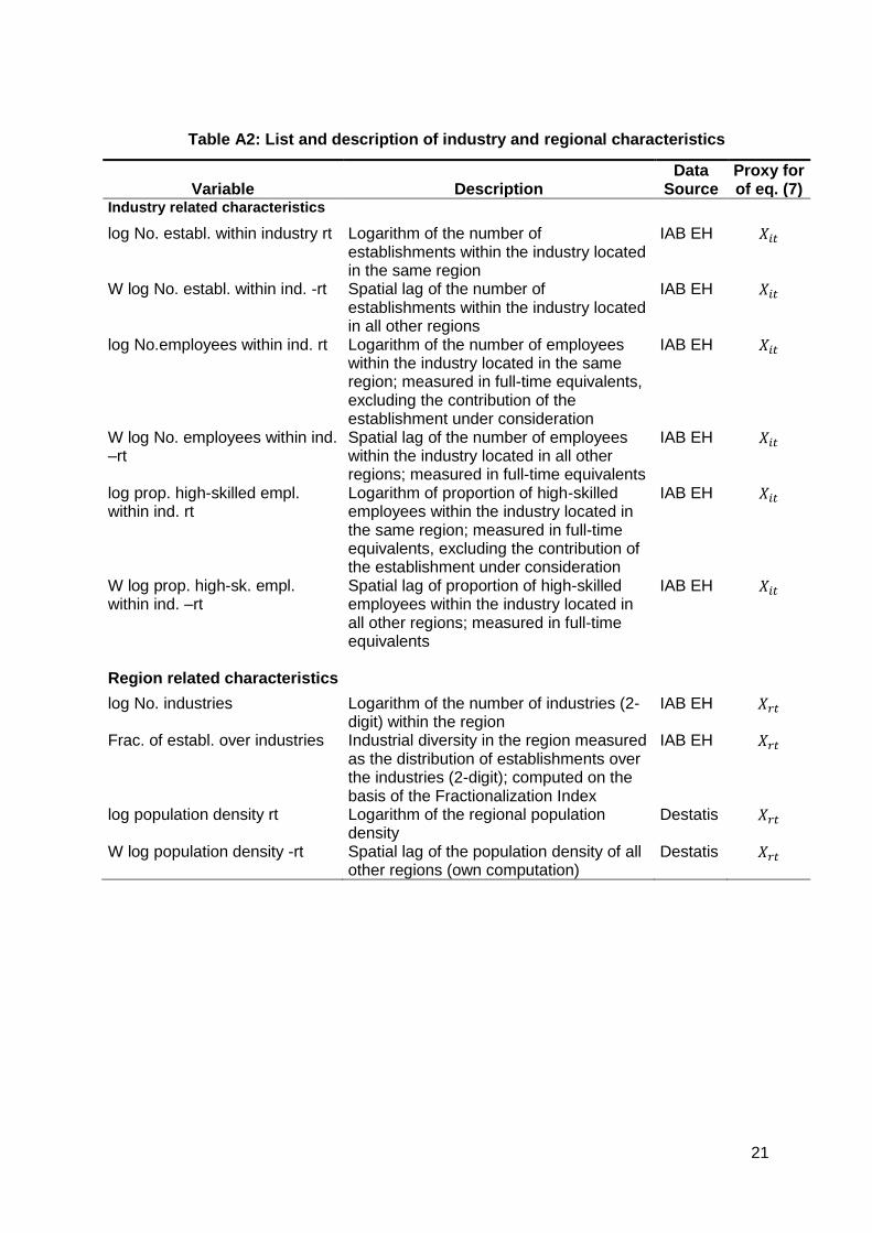
An overview of the variables included in the empirical study with a brief description is
provided in the Appendix in the Table A1 for establishment characteristics and Table A2 for
industry and regional variables.
5. Results
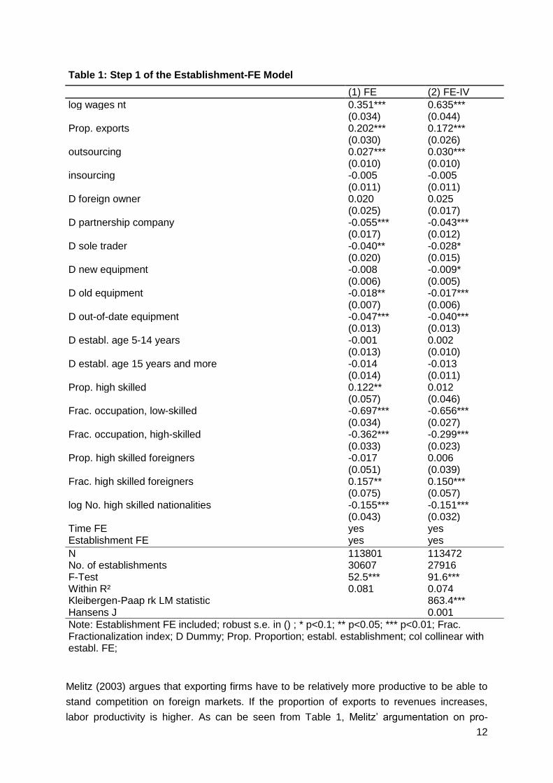
Table 1 contains the first step regressions of Model 1. The first column contains the result of
a standard fixed effects (FE) model. All time constant variables disappear due to the fixed
effects (within) transformation. In the second column wages are instrumented. The tests
show that the IV model does not suffer under weak instruments. The Hansen J test indicates
that the instruments are valid. Reported standard errors are robust to the presence of
arbitrary heteroskedasticity. Model 2 is also estimated. Since the results differ only slightly
from those of Modell 1, they are not reported.
In Table 1 the estimated coefficients reveal the expected signs. The coefficient of wages is
0.351 in the fixed effects regression and 0.635 in the instrumental variables estimation, which
corresponds to the underlying theory. The results suggest that labor and capital are rather
complements than substitutes, because the estimate is less than 1. Considering the
employment structure, we find a significant and positive effect of the high-skilled workers
employed. The effect becomes insignificant when wages are instrumented. This is not
surprising as wages already capture human capital effects: if there are relatively more highly
skilled employees then wages are expected to be higher. As wages are also instrumented
with lagged values, the skill-information is partly included in the instrument. For that reason,
the estimate of the wage rate increases to 0.6, which is an estimate frequently found in
empirical analyses.
12
Table 1: Step 1 of the Establishment-FE Model
(1) FE (2) FE-IV
log wages nt 0.351*** 0.635***
(0.034) (0.044)
Prop. exports 0.202*** 0.172***
(0.030) (0.026)
outsourcing 0.027*** 0.030***
(0.010) (0.010)
insourcing -0.005 -0.005
(0.011) (0.011)
D foreign owner 0.020 0.025
(0.025) (0.017)
D partnership company -0.055*** -0.043***
(0.017) (0.012)
D sole trader -0.040** -0.028*
(0.020) (0.015)
D new equipment -0.008 -0.009*
(0.006) (0.005)
D old equipment -0.018** -0.017***
(0.007) (0.006)
D out-of-date equipment -0.047*** -0.040***
(0.013) (0.013)
D establ. age 5-14 years -0.001 0.002
(0.013) (0.010)
D establ. age 15 years and more -0.014 -0.013
(0.014) (0.011)
Prop. high skilled 0.122** 0.012
(0.057) (0.046)
Frac. occupation, low-skilled -0.697*** -0.656***
(0.034) (0.027)
Frac. occupation, high-skilled -0.362*** -0.299***
(0.033) (0.023)
Prop. high skilled foreigners -0.017 0.006
(0.051) (0.039)
Frac. high skilled foreigners 0.157** 0.150***
(0.075) (0.057)
log No. high skilled nationalities -0.155*** -0.151***
(0.043) (0.032)
Time FE yes yes Establishment FE yes yes
N 113801 113472 No. of establishments 30607 27916 F-Test 52.5*** 91.6*** Within R² 0.081 0.074 Kleibergen-Paap rk LM statistic
863.4***
Hansens J 0.001
Note: Establishment FE included; robust s.e. in () ; * p<0.1; ** p<0.05; *** p<0.01; Frac. Fractionalization index; D Dummy; Prop. Proportion; establ. establishment; col collinear with establ. FE;
Melitz (2003) argues that exporting firms have to be relatively more productive to be able to
stand competition on foreign markets. If the proportion of exports to revenues increases,
labor productivity is higher. As can be seen from Table 1, Melitz’ argumentation on pro-

13
ductivity and trade is supported. If the equipment and machinery employed in the production
process matures, establishment’s productivity decreases. This might reflect the progress of
the product life cycle but also productivity disadvantages of old equipment. In relation to the
product life cycle and therefore to establishments age, we do not find any significant effect of
aging. If the establishment matures it does not become more or less productive.
Focusing on occupational diversity among employment groups we provide evidence that a
rather diverse set of employees goes along productivity losses. This does not seem to be
plausible at first. However, if the fragmentation of occupations is too strong, it is likely that the
establishment is not really focused on a specific task/ production process and therefore
disadvantaged with respect to labor productivity. As expected, this disadvantageous effect is
smaller for highly-skilled occupations.
Considering cultural diversity of high-skilled employees, we support earlier findings of
Brunow and Blien (2014), which focus on overall diversity. However, according to Brunow
and Nijkamp (2012) productivity differences due to cultural diversity of low-skilled people do
not occur and correspondingly we find only evidence for the high-skilled group. The
proportion of employed foreigners is insignificant. Thus, on average there is no negative
effect of employing foreigners in general. However, an increase in the number of nationalities
has negative effects.
Many more variables are important to control in order to assess properly the existence and
the size of agglomeration effects. These variables, however, are time-constant or nearly time
constant. Therefore, these variables are included in the second step of the regression. The
two models of Table 1 do not differ in terms of interpretation. Because the IV model is
adjusted for the endogeneity of wages, it is preferred. From this regression we compute the
establishment fixed effect which now becomes the response variable in the regression of
step 2.
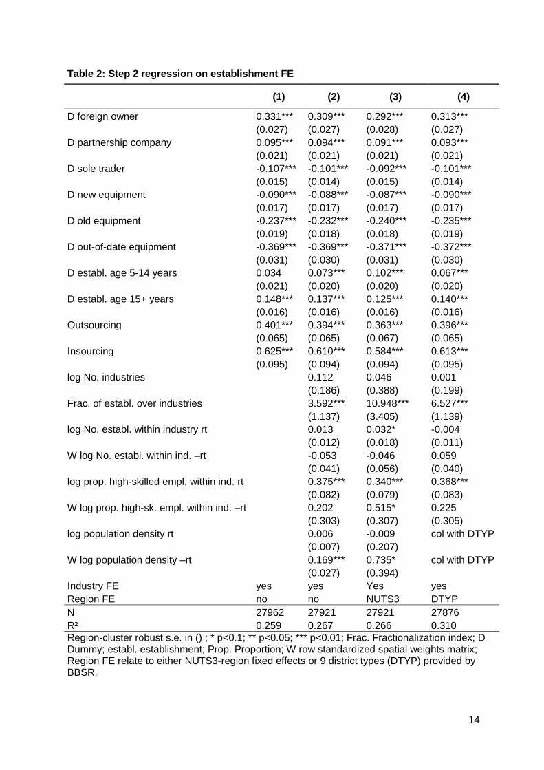
The results of the second step are presented in Table 2. The explanatory variables are
computed by the time average of each variable when the individual establishment is
observed. Depending on the specification, there are about 30,000 distinct establishments
surveyed over time. In all models of Table 2 industry fixed effects are included, as the
theoretical model suggests. Reported standard errors are clustered at the regional level to
take likely correlation among establishments within the region into account. Individual cases
are weighted according to the frequency they are observed.
The first column is a baseline specification which controls for (almost) time constant
establishment characteristics. In column 2 additionally intra-industrial regional variables and
pure regional variables are included to identify the presence of localization and urbanization
economies. The estimates presented in column 3 take additionally region fixed effects into
account and column 4 considers 9 different district types by means of dummy variables
instead of region fixed effects. Parameters do not vary much between this and augmented
models controlling for the regional and industrial environment presented in column (2) to (4).
We therefore conclude that establishment characteristics and the environment characteristics
are almost uncorrelated.
14
Table 2: Step 2 regression on establishment FE
(1) (2) (3) (4)
D foreign owner 0.331*** 0.309*** 0.292*** 0.313***
(0.027) (0.027) (0.028) (0.027)
D partnership company 0.095*** 0.094*** 0.091*** 0.093***
(0.021) (0.021) (0.021) (0.021)
D sole trader -0.107*** -0.101*** -0.092*** -0.101***
(0.015) (0.014) (0.015) (0.014)
D new equipment -0.090*** -0.088*** -0.087*** -0.090***
(0.017) (0.017) (0.017) (0.017)
D old equipment -0.237*** -0.232*** -0.240*** -0.235***
(0.019) (0.018) (0.018) (0.019)
D out-of-date equipment -0.369*** -0.369*** -0.371*** -0.372***
(0.031) (0.030) (0.031) (0.030)
D establ. age 5-14 years 0.034 0.073*** 0.102*** 0.067***
(0.021) (0.020) (0.020) (0.020)
D establ. age 15+ years 0.148*** 0.137*** 0.125*** 0.140***
(0.016) (0.016) (0.016) (0.016)
Outsourcing 0.401*** 0.394*** 0.363*** 0.396***
(0.065) (0.065) (0.067) (0.065)
Insourcing 0.625*** 0.610*** 0.584*** 0.613***
(0.095) (0.094) (0.094) (0.095)
log No. industries
0.112 0.046 0.001
(0.186) (0.388) (0.199)
Frac. of establ. over industries
3.592*** 10.948*** 6.527***
(1.137) (3.405) (1.139)
log No. establ. within industry rt
0.013 0.032* -0.004
(0.012) (0.018) (0.011)
W log No. establ. within ind. –rt
-0.053 -0.046 0.059
(0.041) (0.056) (0.040)
log prop. high-skilled empl. within ind. rt
0.375*** 0.340*** 0.368***
(0.082) (0.079) (0.083)
W log prop. high-sk. empl. within ind. –rt
0.202 0.515* 0.225
(0.303) (0.307) (0.305)
log population density rt
0.006 -0.009 col with DTYP
(0.007) (0.207)
W log population density –rt
0.169*** 0.735* col with DTYP
(0.027) (0.394)
Industry FE yes yes Yes yes
Region FE no no NUTS3 DTYP
N 27962 27921 27921 27876
R² 0.259 0.267 0.266 0.310
Region-cluster robust s.e. in () ; * p<0.1; ** p<0.05; *** p<0.01; Frac. Fractionalization index; D Dummy; establ. establishment; Prop. Proportion; W row standardized spatial weights matrix; Region FE relate to either NUTS3-region fixed effects or 9 district types (DTYP) provided by BBSR.
15
For the control variables, which characterize individual establishments and are (nearly) time-
constant, the expected results are obtained. From the three categories “Partnership
company”, “Sole trader” and “Joint stock capital/ Capital Company” the latter one is the
reference category. The Dummy “sole trader” is negatively, the dummy “Partnership
company” positively significant. Of the variables characterizing the capital equipment of an
establishment all the dummies indicating its age are negatively significant compared to the
category “newest equipment”. A foreign owner is associated with a higher productivity.
If parts of the establishment were outsourced, labor productivity is higher. Of course, the
rational of outsourcing is to be more competitive and if the outsourced service or product can
be bought cheaper compared to self-making, labor productivity of the ‘slim’ establishment will
increase. The same argument holds for insourcing. If transaction costs with another firm are
on average higher than doing the relevant production process in the own establishment,
productivity is expected to be higher.
We now ask whether the establishment effects are influenced by agglomeration forces while
controlling for a variety of fixed effects and time constant establishment characteristics. The
inclusion of the latter variables makes it even harder for agglomeration variables to become
significant. Considering the agglomeration variables it is revealed that a larger number of
industries within the region does not matter. The result might be driven by the fact that the
variation of the number of industries measured at the 2 digit level between regions is
relatively small. However, the fractionalization of industries within a region matters: in regions
where the number of operating establishments is rather equally distributed over industries
labor productivity is higher, on average. Both measures relate to a special form of
urbanization externalities, namely to Jacobs’ effects. It is an important result that the diversity
of the industrial composition matters for productivity. We also tested interaction effects of
both variables, which, however, were insignificant.
Another measure of urbanization is the population density. In the pooled regressions the
estimated coefficients are positive and significant. Thus, an establishment located in markets
with a population concentration has higher labor productivity. There is also a spatial lag of
the population density of the surrounding regions included. That is, not only the market size
of the own region but also of the regions nearby explain labor productivity differences. In the
New Economic Geography literature the population density serves as a measure of demand.
It is frequently argued that being closer to larger markets enhances demand which is
associated with increasing returns and thus, with higher productivity. The estimates on
population density support this argument. In the Fixed Effects Models the between-region
variation is lost and because the population density is rather time constant, it is not surprising
that the effect now becomes insignificant. As a robustness check we employ the size of
regional population instead of population density and find also a positive effect.
There are variables included which are related to Marshall-Arrow-Romer agglomeration
forces within an industry. The number of establishments located in the region (and its spatial
lag) is a measure of the bulk of production taking place in these locations. The variable also
indicates production chains. Finally, it serves as a measure of the intensity of competition. It
16
is insignificant in the basic regression without regional fixed effects but becomes significant in
the FE model. If more establishments of a specific industry locate within the region, average
labor productivity increases. Thus, supply chains and stronger competition within a regional
industry are related to labor productivity gains.
As an alternative measure we use the employment levels and their spatial lag, excluding the
employment level of the establishment under consideration (results are not shown). The
results provide a similar picture as the number of establishments in terms of significance and
direction. A larger workforce employed in a specific industry is associated with labor
productivity gains. It can be argued that this effect is due to common labor markets and
spillover effects. Both variables, the number of establishments and the employment levels –
and their spatial lags, which are not significant – relate to MAR externalities. We also include
both variables in a regression, but the picture does not change much, though both variables
are collinear and the spatial variables become highly significant with the opposite sign.
As a last set of variables we include the intra-industrial proportion of highly-skilled workers,
excluding the contribution of the establishment under consideration. The variable serves as a
proxy of intra-industrial knowledge spillovers and knowledge intensity. This variable is
significant and positive in all models. Establishments located in an environment of knowledge
intense competitors within an industry are on average more productive. This is an important
result, which can also be related to endogenous growth theory which suggests knowledge
spillovers between firms as a key driver of growth.
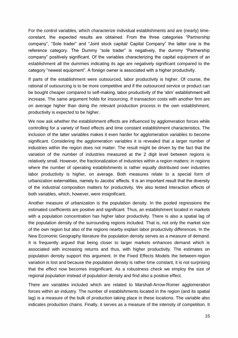
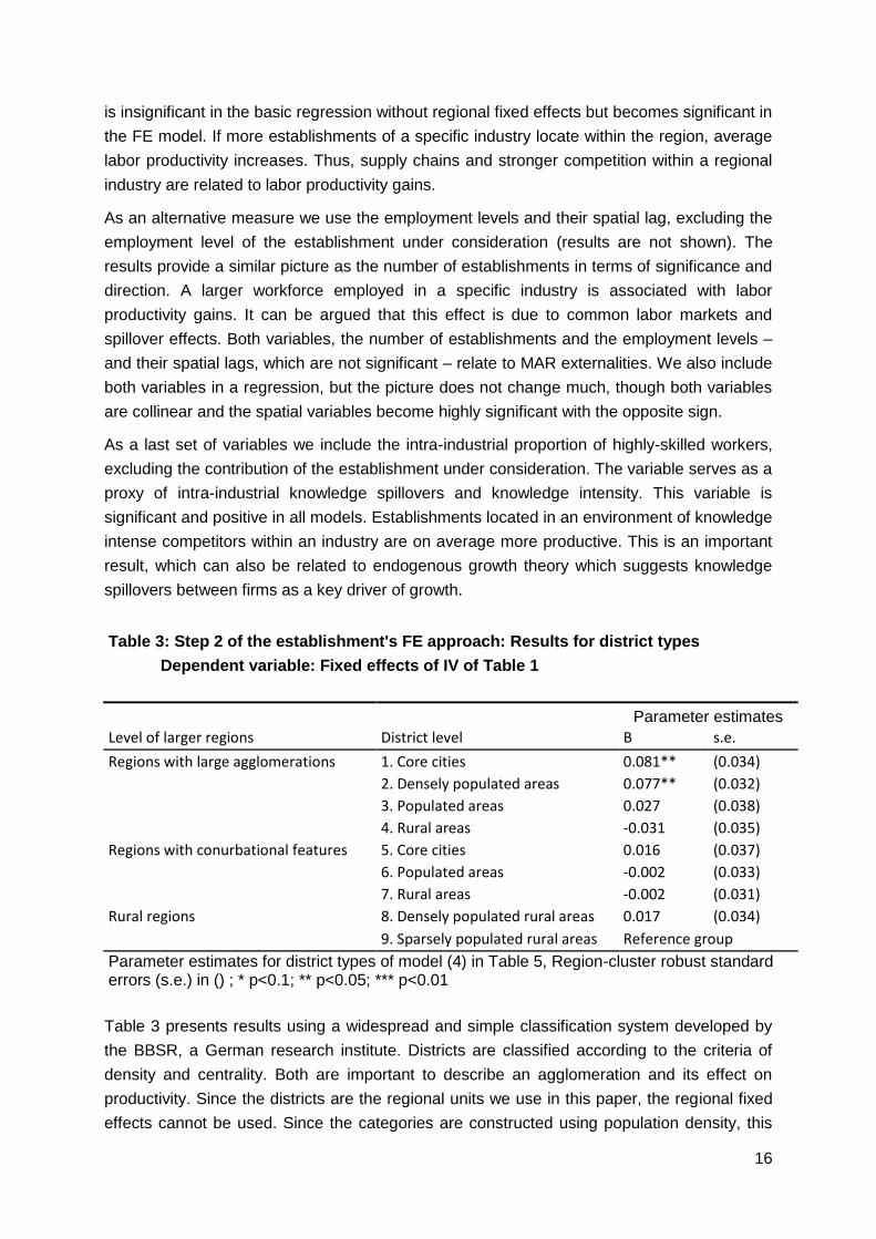
Table 3: Step 2 of the establishment's FE approach: Results for district types
Dependent variable: Fixed effects of IV of Table 1
Parameter estimates
Level of larger regions District level B s.e.
Regions with large agglomerations 1. Core cities 0.081** (0.034)
2. Densely populated areas 0.077** (0.032)
3. Populated areas 0.027 (0.038)
4. Rural areas -0.031 (0.035)
Regions with conurbational features 5. Core cities 0.016 (0.037)
6. Populated areas -0.002 (0.033)
7. Rural areas -0.002 (0.031)
Rural regions 8. Densely populated rural areas 0.017 (0.034)
9. Sparsely populated rural areas Reference group
Parameter estimates for district types of model (4) in Table 5, Region-cluster robust standard errors (s.e.) in () ; * p<0.1; ** p<0.05; *** p<0.01
Table 3 presents results using a widespread and simple classification system developed by
the BBSR, a German research institute. Districts are classified according to the criteria of
density and centrality. Both are important to describe an agglomeration and its effect on
productivity. Since the districts are the regional units we use in this paper, the regional fixed
effects cannot be used. Since the categories are constructed using population density, this
17
variable cannot be included in the regression model. All other control variables as presented
in Table 2 are used. The classification system takes control of regional effects in ‘similar’
regions, but is less restrictive than the pure region fixed effects model.
The coefficients of the other variables are not shown, because they are nearly unchanged by
the switching of approaches. However, there are significant differences between regional
types. The more remote a region is the less productive are establishments. An establishment
located in a rural region which is closer to a metropolitan area is relatively more productive
compared to an establishment located in a rural region in a sparsely populated area. Thus,
centrality also matters for productivity differentials. The most productive regions are those in
the center of a metropolitan area.
6. Conclusion
One of the crucial questions of regional economics concerns the existence of agglomeration
effects. These are expected due to the “Marshallian forces”: common labor markets,
knowledge spillovers, forward and backward linkages between firms or establishments foster
higher productivity in areas more densely populated by firms and by people. Though there
has been much research on the existence of these forces most of the empirical studies were
affected by limitations concerning the units of observations. Most of the studies operate at an
aggregate level which does not allow a precise measurement of agglomeration forces. In this
study data of individual establishments are used to assess the effects expected from
theoretical considerations.
The empirical part of this paper shows in detail that agglomeration effects are present.
Localization forces and urbanization forces are both important. The metropolitan areas are
those regions which are the engines of productivity in the country. Regions have differential
consequences for the establishments located in their territories. Densely populated
metropolitan areas are those whose establishments reach the highest levels of labor
productivity, whereas rural regions outside agglomerations are disadvantaged. The analysis
for district types shows that this conclusion is justified even within a metropolitan area.
Establishments located closely to the core of an agglomeration are not as productive as are
those which are placed exactly in the core. Our approach uses relatively small regional units
which facilitates the identification of these differences.
The conclusion concerning agglomeration forces can be drawn even after controlling
important individual level variables. The respective industry and the modernity of the
production equipment obviously influence the productivity of a firm. However, the effect of
concentration of economic activity remains after controlling for these variables. Therefore the
approach chosen makes it possible to have a closer look at the forces which are effective in
the interaction between regions and establishments. The conclusion is that the location of an
establishment influences its productivity. Besides various forms of concentration which can
be shown of having an effect, also the diversity of a region is important. Therefore, not only
Marshall-Arrow-Romer effects are present, especially knowledge spillover, but also Jacobs
effects.

18
Literature Autor D H, F Levy, R J Murnane (2003): The Skill Content of Recent Technological Change: An Empirical Exploration. The Quarterly Journal of Economics 118 (4), 1279-1333. Baldwin R E (1999): Agglomeration and endogenous capital. European Economic Review 43, 263-280. Baldwin J, M Brown, D Rigby (2010): Agglomeration Economies: Microdata Panel Estimates from Canadian Manufacturing. Journal of Regional Science 50 (5), 915-934. Baldwin R E, T Okubo (2006): Heterogeneous firms, agglomeration and economic geography: spatial selection and sorting. Journal of Economic Geography 6, 323-346. Bell B, S Nickell, G Quintini (2002): Wage equations, wage curves and all that. Labour Economics 9, 341-360. Benfratello L, A Sembenelli (2006): Foreign ownership and productivity: Is the direction of causality so obvious? International Journal of Industrial Organization 24 (4), 733-751. Blien U, H Sanner (2014): Technological Progress and Employment. Economics Bulletin 34
(1), 245-251. Blien U, H Gartner, H Stüber, K Wolf (2009): Regional price levels and the agglomeration wage differential in western Germany. Annals of Regional Science 43 (1), 71-88. Brunow S, U Blien (2014): Effects of Cultural Diversity on Individual Establishments. International Journal of Manpower, 35, 166-186. Brunow S, G Hirte (2009): Regional Age Pattern of Human Capital and Regional Productivity: A Spatial Econometric Study on German Regions. Papers in Regional Science 88, 799-823. Brunow S, V Nafts (2013): What types of firms tend to be more innovative: a study on Germany. Norface migration discussion paper, 2013-21, London, 25 S. Brunow S, P Nijkamp (2014): The impact of a culturally diverse workforce on firms' market size: an empirical investigation on Germany. International Regional Science Review, forthcoming. Card D (1995): The Wage Curve: A Review. Journal of Economic Literature 33 (2), 785-799.
Combes P-P, T Magnac, J.M Robin (2004): The Dynamics of Local Employment in France. Journal of Urban Economics 56, 217-243.
Drucker J, E Feser (2012): Regional industrial structure and agglomeration economies: An analysis of productivity in three manufacturing industries. Regional Science and Urban Economics 42 (1-2), 1-14. Duncan J, S Hoffmann (1981): Overeducation, undereducation, and the theory of career mobility. Applied Economics 36, 803-816. Gathmann C, U Schönberg (2010): How general is human capital? A task-based approach. Journal of Labor Economics 28 (1), 1-49.

19
Glaeser E, G Ponzetto, K Tobio (2011): Cities, skills, and regional change. NBER Working Paper 16934. Görmar W, E Irmen (1991): Nichtadministrative Gebietsgliederungen und -kategorien für die Regionalstatistik. Die siedlungsstrukturelle Gebietstypisierung der BfLR", in: Raumforschung und Raumordnung 49/6: 387-394, updated version available under http://www.bbsr.bund. de/BBSR/DE/Raumbeobachtung/Raumabgrenzungen/SiedlungsstrukturelleRegionstypenEuropa/NUTS3Zus/NUTS3TypenZusamm.html Greene, W. (2011): Fixed Effects Vector Decomposition: A Magical Solution to the Problem of Time-Invariant Variables in Fixed Effects Models? Political Analysis (19),135-146. Henderson J V (2003): Marshall’s scale economies. Journal of Urban Economics 53, 1-28. Jacobs J (1969): The Economy of Cities, Random House, New York. Krugman P (1991): Increasing returns and economic geography. Journal of Political Economy 99, 483-499. Marshall A (1997): Principles of Economics (originally published 1920), Amherst: Prometheus Books. Melitz M (2003): The Impact of Trade on Intra-Industry Reallocations and Aggregate Industry Productivity. Econometrica 71 (6), 1695-1725. Moretti E (2004): Education, spillovers and productivity. American Economic Review 94 (3), 656-690. Plümper T, V E Troeger (2007): Efficient Estimation of Time-Invariant and Rarely Changing Variables in Finite Sample Panel Analyses with Unit Fixed Effects. Political Analysis (15), 124-139. Rosenthal S, W Strange (2004): Evidence on the nature and sources of agglomeration economies. In: J. V. Henderson & J. F. Thisse (ed.): Handbook of Regional and Urban Economics 4, chapter 49, 2119–2171, Elsevier. Spitz-Öner A (2006): Technical Change, Job Tasks, and Rising Educational Demands: Looking Outside the Wage Structure. Journal of Labor Economics 24, 235-70. Trax M, S Brunow, J Suedekum (2012): Cultural diversity and plant level productivity, IZA discussion paper, 6845.
20
Appendix
Table A1: List and description of establishment characteristics
Data Proxy for Variable Description Source eq. (7)
D foreign owner Foreign ownership (yes/no) IAB EP D partnership company Partnership company (yes/no) IAB EP D sole trader Sole trade (yes/no) IAB EP D establ. age 5-14 years Establ. age between 5-14 years (Dummy) IAB EH D establ. age 15+ years Establ. age 15 years and more (Dummy) IAB EH Outsourcing Parts of the establ. were outsourced
(yes/no) IAB EP
Insourcing Parts of the establ. were insourced (yes/no)
IAB EP
D new equipment Establ. operates with new equipment (Dummy, reference: newest equipment)
IAB EP
D old equipment Establ. operates with rather old equipment (Dummy, reference: newest equipment)
IAB EP
D out-of-date equipment Establ. operates with out-of-date equipment(Dummy, reference: newest equipment)
IAB EP
log wages nt Logarithm of average daily wages paid to employees
IAB EH
Prop. exports Proportion of exports on revenues IAB EP Prop. high skilled Proportion of high-skilled employees IAB EH Frac. occupation, low-skilled; Frac. occupation, high-skilled
Establishments diversity of employment over occupations employed within the group of low-skilled (high-skilled) employees; computed on the basis of the Fractionalization index
IAB EH
Prop. high skilled foreigners Proportion of high-skilled foreigners on all employed high-skilled workers
IAB EH
Frac. high skilled foreigners Diversity of high-skilled foreigners over nationalities; computed on the basis of the Fractionalization index
IAB EH
log No. high skilled nationalities Logarithm of the total number of foreign nationalities employed (zero for establishments without high-skilled foreign employees
IAB EH
21
Table A2: List and description of industry and regional characteristics
Data Proxy for Variable Description Source of eq. (7)
Industry related characteristics
log No. establ. within industry rt Logarithm of the number of establishments within the industry located in the same region
IAB EH
W log No. establ. within ind. -rt Spatial lag of the number of establishments within the industry located in all other regions
IAB EH
log No.employees within ind. rt Logarithm of the number of employees within the industry located in the same region; measured in full-time equivalents, excluding the contribution of the establishment under consideration
IAB EH
W log No. employees within ind. –rt
Spatial lag of the number of employees within the industry located in all other regions; measured in full-time equivalents
IAB EH
log prop. high-skilled empl. within ind. rt
Logarithm of proportion of high-skilled employees within the industry located in the same region; measured in full-time equivalents, excluding the contribution of the establishment under consideration
IAB EH
W log prop. high-sk. empl. within ind. –rt
Spatial lag of proportion of high-skilled employees within the industry located in all other regions; measured in full-time equivalents
IAB EH
Region related characteristics
log No. industries Logarithm of the number of industries (2-digit) within the region
IAB EH
Frac. of establ. over industries Industrial diversity in the region measured as the distribution of establishments over the industries (2-digit); computed on the basis of the Fractionalization Index
IAB EH
log population density rt Logarithm of the regional population density
Destatis
W log population density -rt Spatial lag of the population density of all other regions (own computation)
Destatis