Age-depth modelling part 1

0 random walk proxy simulations

1 Calibration of 14C dates

2 Basic 14C age-depth modelling

Schedule flexible and interactive! Focus on uncertainty

R

Stats and graphing software

Many user-provided modules

Free, open-source

Open R and type:

plot(1:10, 11:20)

x <- 1:10 ; y <- 11:20 ; plot(x, y, type='l')

Case sensitive

Previous commands: use up cursor

Random walk simulations

Check http://chrono.qub.ac.uk/blaauw/Random.R in browser

Open R and load the link:

Source ( url( 'http://chrono.qub.ac.uk/blaauw/Random.R' ) )

RandomEnv()

RandomEnv(nforc=2, nprox=5)

RandomProx()

Introduction – 14C decay

Atm. 12C (99%), 13C (1%), 14C (10-12) 14C decays exponentially with time Cease metabolism -> clock starts ticking Measure ratio 14C/C to estimate age fossil

Calibrate – 14C age errors

Counting uncertainty AMS Counting time (normal vs high-precision dates) Sample size (larger = more 14C atoms) Drift machine (need to correct, standards)

Preparation samples Pretreatment, chemical & graphitisation Material-dependent (e.g. trees, bone, coral) Lab-specific

Every measurement will be bit different Errors assumed to have Normal distribution

14C dating

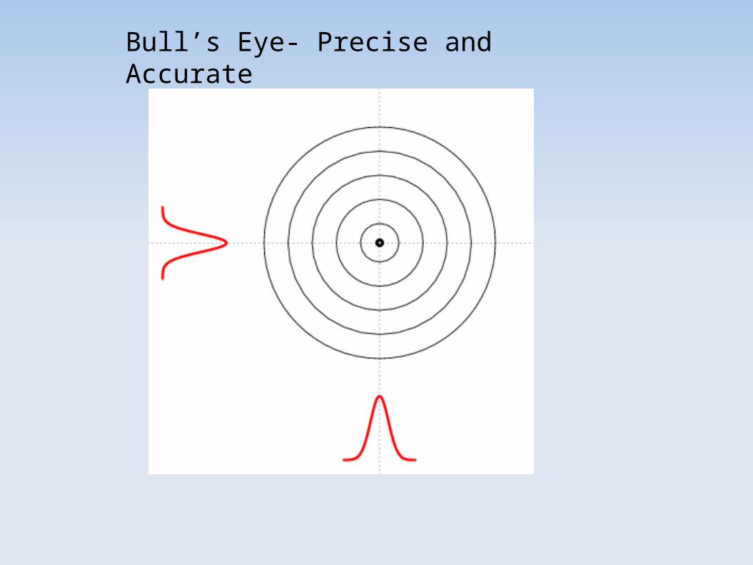
Bull’s Eye- Precise and Accurate

Precise but inaccurate

Accurate (on average) but imprecise

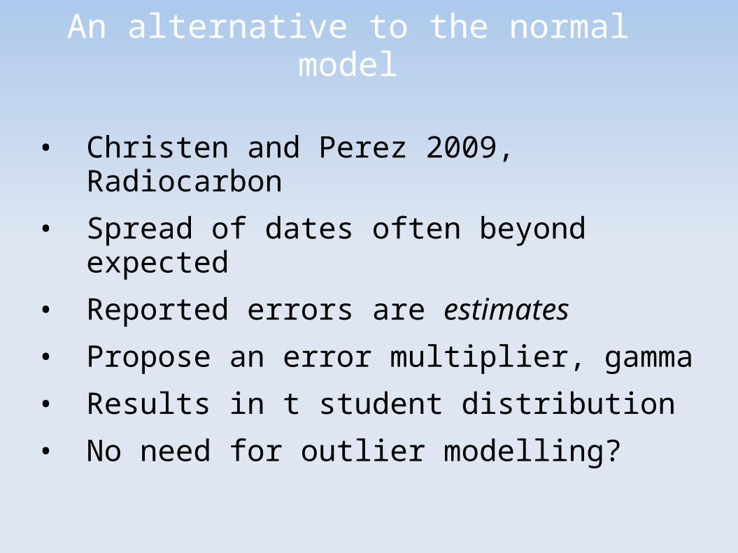
An alternative to the normal model

• Christen and Perez 2009, Radiocarbon

• Spread of dates often beyond expected

• Reported errors are estimates

• Propose an error multiplier, gamma

• Results in t student distribution

• No need for outlier modelling?

http:///www.chrono.qub.ac.uk/blaauw/

14C calibration

Calibrate - methods

Probability preferred over intercept Less sensible to small changes in mean Resulting cal.ranges make more sense

Procedure probability method: What is prob. of cal.year x, given the date? Calculate this prob. for all cal.ages

Combine errors date and cal.curve √(2+sd2)

Calibrate - methods

Multimodal distributions Which of the peaks most likely (Calib %)? How report date?

1 or 2 sd sd range mean±sd mode weighted mean (Telford et al. ‘05 Holocene) why not plot the entire distribution!

Calibration, the equations

• Calibration curve provides 14C ages µ for calendar years θ, µ(θ)

• 14C measurement y ~ N(mean, sd)

• Calibrate: find probability of y for θ

N( µ(θ) , σ ), where σ2 = sd2 + σ(θ)2

for sufficiently wide range of θ

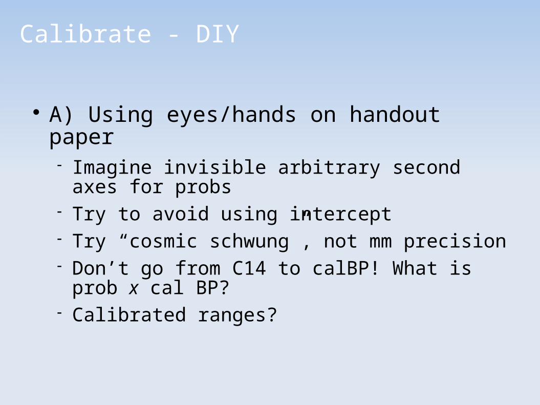
Calibrate - DIY

A) Using eyes/hands on handout paper Imagine invisible arbitrary second axes for

probs Try to avoid using intercept Try “cosmic schwung”, not mm precision Don’t go from C14 to calBP! What is prob x

cal BP? Calibrated ranges?

1. clam ... R

R works in “workspace” Remember where you work(ed)! Change working dir via File > Change

Dir Or permanently using Desktop Icon

(right-click, properties, start in) Change R to your Clam workspace

1. Calibrating DIY

Define years: yr <- 1:1000 A date: y <- 230; sdev <- 70 Prob. for each yr: prob < - dnorm(yr, y,

sdev) plot(yr, prob, type=‘l’) But we should calibrate: cc <-

read.table(“IntCal09.14C”, header=TRUE) cc[1:10,] prob <- dnorm(cc[,2], y,

sqrt(sdev^2+cc[,3]^2)) plot(cc[,1], prob, type='l', xlim=c(0,

1000) )

Calibrate - DIY

clam (Blaauw, in press Quat Geochr) Open R (via desktop icon or Start menu) Change working directory to clam dir Type: source(''clam.R'') [enter] Type: calibrate(130, 35)

2. clam, calibrating

Type calibrate() This calibrated 14C date of 2450 +- 50 BP Type calibrate(130, 30) Type calibrate(130, 30, sdev=1) Try calibrating other dates, e.g., old ones All clam code is open source, you can

read the code to see/follow what it does

Feedback please

• What was for you the best way to understand 14C calibration? Why?– Dedicated software (OxCal, Calib, clam)

– Draw by hand

– Animations

– Equations