aerosol lidar for continuous atmospheric monitoring

ISSN 1024�8560, Atmospheric and Oceanic Optics, 2013, Vol. 26, No. 4, pp. 308–319. © Pleiades Publishing, Ltd., 2013.Original Russian Text © I.A. Razenkov, 2013, published in Optica Atmosfery i Okeana.

308

1. PROBLEM STATEMENT

An aerosol lidar is an instrument whose operationis based on radiation scattering by molecules and par�ticles. The lidar consists of a pulsed laser and a receiv�ing telescope; it is used for remote detection of atmo�spheric particles and measurements of scattering coef�ficients p[1, 2]. A diode�pumped laser with high pulserepetition rate and low pulse energy is preferable foruse in continuous monitoring. A lidar with a laser witha pulse repetition rate of several kHz and pulse energyof less than 1 mJ is called micropulse lidar. Such sys�tems are safe for human eyes.

The most popular eye�safe micropulse lidar wasdesigned by NASA in the beginning of 1990s [3]. Thissystem was called MPL and is sold by the SESI Com�pany. Many of these lidars operate all over the worldwithin the lidar network MPL�Net. A laser beams isbroadened in MPL via a receiving 18�cm telescope(Cassegrain), which is a transceiver. In the first sam�ples, the telescope was assembled in an aluminumpipe; therefore, the focus position was sensitive to vari�ations in temperature inside a working room. A changein the temperature by 10°C resulted in a 50% andhigher error in measurements of the backscatteringcoefficient [4].

An MPL laser operates at, or close to, a wavelengthof 532 nm; the pulse repetition rate is 2500 Hz, and thepulse energy is 10 μJ. The field�of�view is 100 μrad. Abeam splitting cube and a depolarizer are used as atransmitter�receiver (TR) switch. It does not allowrecording the cross�component of an echo signal anddetermining depolarization, and a half of the powersent to the atmosphere is not used during transmis�sion. “Absolute calibration of the measured profile is

problematic” is written in the part “Absolute calibra�tion” in the Micropulse Lidar Handbook [5].

A usual calibration procedure for determining adependence between the instrument indications andparameters measured cannot be used for the lidar,since the lidar records the echo signal PΣ equal to thesum of the molecular Pm (Rayleigh scattering) andaerosol Pa (Mie scattering) signals. The problem oflidar calibration is solved only if there is a molecularreceiving channel.

Let us write the lidar equation for the echo signalpower (total receiving channel) as

(1)

where r is the distance; P is the average power of a laserpulse of Δtp in length; ηΣ is the receiver efficiency; G(r)is the geometric function of the lidar; A is the area ofthe receiving telescope; c is the speed of light; βm(r) isthe molecular backscattering coefficient; βa(r) is the

aerosol backscattering coefficient; is

the atmospheric optical depth; and α(r) is the attenu�ation coefficient. If the radiation absorption isneglected, then the coefficient α(r) is a sum of thecoefficients of the total molecular αm(r) and totalaerosol αa(r) scattering.

There are two unknown variables in Eq. (1), i.e.,the backscattering coefficient βa(r) and the total aero�sol scattering coefficient αa(r). A correlation betweenthese coefficients is not universal; therefore, it is usu�

( ) ( )

Σ Σ= + = η

Δ× β + β τ

p2

( ) ( ) ( ) ( )

( ) ( ) exp –2 ( ) ,2

m a

m a

P r P r P r P G r

c tA r r rr

' '

0

( ) ( )

r

r r drτ = α∫

Aerosol Lidar for Continuous Atmospheric MonitoringI. A. Razenkov

V.E. Zuev Institute of Atmospheric Optics, Siberian Branch, Russian Academy of Sciences, pl. Akademika Zueva 1, Tomsk, 634021 Russia

Received April 23, 2012

Abstract—A design is proposed of an eye�safe high spectral resolution lidar operating at a wavelength of532 nm. Absolute calibration is ensured by a molecular channel where aerosol signals are filtered in an iodine�filled cell. Laser beam expansion in a transmitter via a receiving telescope ensures high thermo�mechanicalstability of the design, which allows a small field�of�view and substantial reduction of the background noiselevel. A detailed optical circuit of the transceiver is shown, where the transmitter and the receiver are locatedon different sides of the optical bench for better stability. Specifications of the laser and the system are given.Lidar returns are calculated, and measurement errors are estimated. It is shown that the time of averagingshould be no longer than 1 min to attain 10% accuracy when calculating the aerosol backscattering coefficientand optical depth in the troposphere. The system proposed is to operate continuously and unattended.

DOI: 10.1134/S1024856013040118

OPTICAL INSTRUMENTATION

ATMOSPHERIC AND OCEANIC OPTICS Vol. 26 No. 4 2013

AEROSOL LIDAR FOR CONTINUOUS ATMOSPHERIC MONITORING 309

ally defined using different models [6, 7] for solutionof Eq. (1) when sounding with a simple aerosol lidar,and the result depends on a model chosen.

To calibrate the lidar, i.e., to find the absolute valueof the aerosol backscattering coefficient βa(r), themolecular scattering coefficient βm(r) should be used,which can be calculated if the air temperature isknown [8]. The molecular signal Pm(r), correspondingto the coefficient βm(r), should also be measured. Anequation for the molecular echo signal Pm(r) differsfrom Eq. (1) in the absence of βa(r) and the presenceof ηm instead of ηΣ, which characterizes the receiverefficiency in the molecular channel:

(2)

An equation for the aerosol backscattering coeffi�cient βa(r) can be derived from a ratio of signals (1)and (2) multiplied by βm(r):

(3)

One can say that the aerosol lidar is calibrated by themolecular scattering. In this case, the lidar as aninstrument for measuring atmospheric parameters willbe calibrated in legal units of the SI system, whichensures the uniformity of measurement units used inall fields of science and technology.

A profile of the optical air density τ(r) is definedfrom Eq. (2) by finding a logarithm of the ratio of themolecular signal Pm(r) to the molecular scatteringcoefficient βm(r):

(4)

where r0 is the distance near the lidar (about 100 m);Pm(r0), Gm(r0), and βm(r0) are the normalization fac�tors.

There are two types of lidar systems capable ofrecording molecular signals: Raman lidars [9] andhigh spectral resolution lidars (HSRLs) [10]. Systemsof the first type record a signal the frequency of whichis significantly shifted due to the Raman scattering,and about 0.1% of the whole molecule�scatteredenergy is contained in this signal. These systems arerelatively simple, but bulky, because they require ahigh�power laser and a large telescope due the smallcross�section of the Raman scattering. Raman lidarscan not be eye�safe.

HSRLs record a Rayleigh scattering signal, thespectrum of which is broadened due to the Dopplereffect when scattered by chaotically moving moleculesand Brillouin scattering by density fluctuations. Thebroadening is very small, some GHz in the visiblespectral region. But this signal contains about 99.9%of all the molecular�scattered energy [8]. These sys�

( )Δ

= η β τp

2( ) ( ) ( )exp –2 ( ) .

2m m m

c tAP r P G r r rr

Σ

Σ

⎛ ⎞ηβ = β ⎜ ⎟η⎝ ⎠

( )( ) ( ) – 1 .

( )m

a mm

P rr r

P r

0 0

0

( ) ( ) ( )1( ) – ln ,2 ( ) ( ) ( )

m m

m m

P r G r rr

P r G r r

⎡ ⎤βτ = ⎢ ⎥β⎣ ⎦

tems are complex, but more compact and more prom�ising in our opinion. A Rayleigh molecular signal wasfirst recorded in 1970 [11].

An incoming signal is divided into two parts in aHSRL. The first part is recorded by a total channel’sdetector. An aerosol signal is subtracted from the sec�ond part of the signal using a band�rejection filter (cellwith iodine vapors), and then the signal is recorded bya molecular channel’s detector. A Doppler shift is lessthan 0.01 nm (8 GHz) in the visible range. Engineer�ing implementation of the technique is possible onlywith the use of a pulsed narrow�bandwidth single�fre�quency injection laser [12].

It is evident that a HSRL is preferable for continu�ous monitoring. We assume that a modern aerosollidar for continuous monitoring is to satisfy the follow�ing requirements: (1) absolute calibration by molecu�lar scattering, (2) eye�safety, (3) high thermo�mechanical stability of the design, (4) long�term(months and years) continuous operation, (5) unat�tended work (online control and data acquisition),(6) small size, and (7) economic feasibility. The aboveproperties allow significant expansion of the fields ofuse of lidar. This lidar can be useful in inland, ship, andaircraft expeditions, in scientific research in distantand inaccessible areas, at weather stations in cities andairports for clouds and visual range monitoring.

2. CHOICE OF THE DESIGN

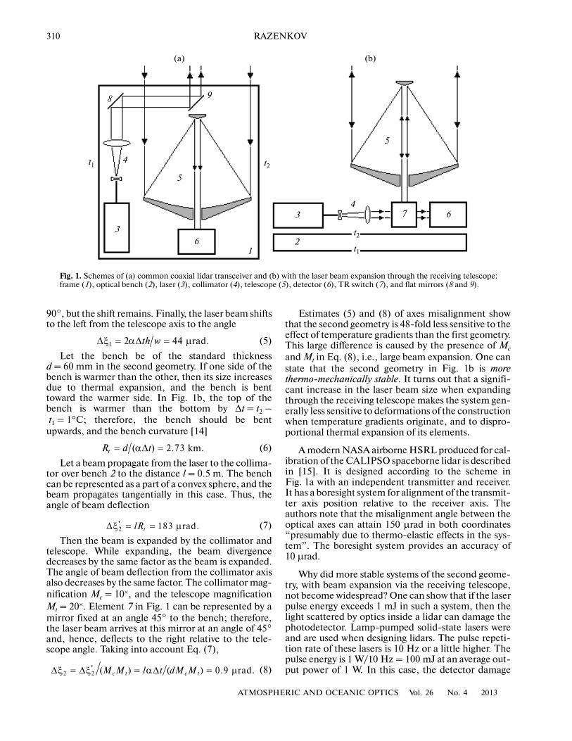
There are two main approaches to designing a lidartransceiver. The first one is the most common, where alaser beam is sent to the atmosphere without passingthrough the receiving part of the system. The axes ofthe beam and the receiving telescope can be close(biaxial scheme) or aligned (coaxial scheme). The sec�ond approach suggests combined use of the telescope,when a laser beam is expended by the receiving tele�scope, which is a transmitter at the same time [13].Figure 1 shows coaxial transceivers in a simplifiedform, with independent beam expansion and with theexpansion via the receiving telescope.

The elements in the first geometry are mounted onframe 1, and in the second geometry, on optical bench 2.Let us estimate the effect of the temperature gradientΔt = t2 – t1 = 1°C, which originates at the edges ofboth geometries, on the misalignment angle Δξbetween the receiver and transmitter axes. Let frame 1and bench 2 be aluminum, i.e., the thermal expansioncoefficient α = 22 × 10–6 1/°C. Frame 1 has the heighth and width w equal to 1 m in the first geometry. Theright side of the frame rises to αΔth = 22 μm due tothermal expansion (t2 > t1). Simultaneously, mirror 8rotates counterclockwise to the angle αΔth/w =22 μrad, and a laser beam reflected from it shifts to thedoubled angle. Mirrors 8 and 9 operate as a periscope;therefore, mirror 9 turns the beam upwards around

310


RAZENKOV

90°, but the shift remains. Finally, the laser beam shiftsto the left from the telescope axis to the angle

(5)

Let the bench be of the standard thicknessd = 60 mm in the second geometry. If one side of thebench is warmer than the other, then its size increasesdue to thermal expansion, and the bench is benttoward the warmer side. In Fig. 1b, the top of thebench is warmer than the bottom by Δt = t2 –t1 = 1°C; therefore, the bench should be bentupwards, and the bench curvature [14]

(6)

Let a beam propagate from the laser to the collima�tor over bench 2 to the distance l = 0.5 m. The benchcan be represented as a part of a convex sphere, and thebeam propagates tangentially in this case. Thus, theangle of beam deflection

(7)

Then the beam is expanded by the collimator andtelescope. While expanding, the beam divergencedecreases by the same factor as the beam is expanded.The angle of beam deflection from the collimator axisalso decreases by the same factor. The collimator mag�nification Mc = 10×, and the telescope magnificationMt = 20×. Element 7 in Fig. 1 can be represented by amirror fixed at an angle 45° to the bench; therefore,the laser beam arrives at this mirror at an angle of 45°and, hence, deflects to the right relative to the tele�scope angle. Taking into account Eq. (7),

(8)

rad.1 2 44th wΔξ = αΔ = μ

km.( ) 2.73tR d t= αΔ =

rad.2' 183tlRΔξ = = μ

rad.2 2' ( ) ( ) 0.9c t c tM M l t dM MΔξ = Δξ = αΔ = μ

Estimates (5) and (8) of axes misalignment showthat the second geometry is 48�fold less sensitive to theeffect of temperature gradients than the first geometry.This large difference is caused by the presence of Mc

and Mt in Eq. (8), i.e., large beam expansion. One canstate that the second geometry in Fig. 1b is morethermo�mechanically stable. It turns out that a signifi�cant increase in the laser beam size when expandingthrough the receiving telescope makes the system gen�erally less sensitive to deformations of the constructionwhen temperature gradients originate, and to dispro�portional thermal expansion of its elements.

A modern NASA airborne HSRL produced for cal�ibration of the CALIPSO spaceborne lidar is describedin [15]. It is designed according to the scheme inFig. 1a with an independent transmitter and receiver.It has a boresight system for alignment of the transmit�ter axis position relative to the receiver axis. Theauthors note that the misalignment angle between theoptical axes can attain 150 μrad in both coordinates“presumably due to thermo�elastic effects in the sys�tem”. The boresight system provides an accuracy of10 μrad.

Why did more stable systems of the second geome�try, with beam expansion via the receiving telescope,not become widespread? One can show that if the laserpulse energy exceeds 1 mJ in such a system, then thelight scattered by optics inside a lidar can damage thephotodetector. Lamp�pumped solid�state lasers wereand are used when designing lidars. The pulse repeti�tion rate of these lasers is 10 Hz or a little higher. Thepulse energy is 1 W/10 Hz = 100 mJ at an average out�put power of 1 W. In this case, the detector damage

(a) (b)

12

3

4

5

6

7

8 9

t1 t2

3

4

5

6

t1

t2

Fig. 1. Schemes of (a) common coaxial lidar transceiver and (b) with the laser beam expansion through the receiving telescope:frame (1), optical bench (2), laser (3), collimator (4), telescope (5), detector (6), TR switch (7), and flat mirrors (8 and 9).



threshold is 100�fold exceeded. Hence, the scheme inFig. 1b is inapplicable.

Continuously pumped diode lasers were designedabout twenty years ago. Their pulse repetition rate isdetermined by the frequency of the gate response andcan attain several tens of kHz. Let the pulse repetitionrate of a diode�pumped laser be equal to 5 kHz, thenthe pulse energy is 1 W/5 kHz = 0.2 mJ at an averageoutput power of 1 W; this is 5�fold lower than thedetector damage threshold. All that said above showsthat a diode�pumped laser is to be used in the design of alidar with beam expansion via the receiving telescope.

There is another very important point. An increasein the pulse repetition rate from 10 Hz to 5 kHz at thesame output power results in a decrease in the energyof sounding pulses by 500 times. Twenty�fold expan�sion of a laser beam in the telescope provides an addi�tional 400�fold decrease in the radiation density at thelidar output. As a result, an increase in the pulse repe�tition rate from 10 Hz to 5 kHz and additional 20�foldexpansion of the beam decrease the radiation densityby 200000 times! This provides a real possibility ofdesigning eye�safe systems.

3. EYE SAFETY

Let us estimate the permissible eye�safe power oflaser radiation at the lidar output. The average poweris determined by the energy of sounding pulses E0 andthe pulse repetition rate f. The maximum laser pulserepetition rate is determined from the condition ofthe presence of only one sounding pulse within the atmo�sphere to avoid uncertainty when recording scatteredradiation. If we assume that aerosol is absent at alti�tudes Hmax higher 30 km, then the pulse repetition ratecan be defined by the equation

(9)

where the factor 2 is caused by direct and back lightpropagation.

Let us now estimate the laser energy parametersrequired for designing eye�safe systems. The calcula�tion is carried out in the visible spectrum. According tothe US standard [16], the maximum permissible expo�sure MPEs for a single pulse of 1 ns–18 μs in length forwavelength from 400 to 700 nm

MPEs = 5 × 10–7 J/cm2. (10)

For the case of a sequence of n pulses, the MPEs

values is corrected, and a new value MPEm is definedas [16]

MPEm = MPEs n–1/4. (11)

The number of pulses n is determined from the condi�tion that an eye requires 0.25 s for closing. For thepulse repletion rate equal to 5 kHz, n = 1250. Then,taking into account Eqs. (10) and (11), we have

MPEm = 8.4 ⋅ 10–8 J/cm2. (12)

kHzmax(2 ) 5 ,f c H= =

Finally, MPEm is the maximally permissible energy ofa laser pulse at the telescope output at a pulse repeti�tion rate of 5 kHz.

Let us now find the laser pulse energy. For this, weshould know the energy distribution of the beamcross�section at the telescope output. Let us considerthis problem for two beam types, i.e., uniform andGaussian. Let us write an equation for energy distribu�tion in general form:

(13)

where x and y are the Cartesian coordinates alignedwith the optical axis of the telescope, Dtel is the tele�scope diameter, and the parameter beam determinesthe beam type:

(14)

Equation (13) implies that the energy density cannotexceed MPEm. The factor 2 in Eq. (13) means that theintensity of a Gaussian beam decreases by e2 times atthe telescope edge.

To determine the maximum permissible pulseenergy E0, Eq. (13) should be integrated over the tele�scope surface. The integration is easier in the polarcoordinates ρ and ϕ:

(15)

where Rblock is the radius of the mount of the secondarymirror of the telescope, which blocks the central partof the main mirror of Rtel in radius. The maximum per�missible power of laser radiation at the lidar output is

P0 = fE0. (16)

Equations (13), (15), and (16) allow calculation ofthe maximum permissible energy of an individual

( )2 2 2

( , , )

exp –2 ( ) ,

m

tel

E x y beam MPE

beam x y D

=

⎡ ⎤× +⎣ ⎦

uniform distribution,

Gaussian distribution.

0 –

1 –beam

⎧= ⎨⎩

0

2

0

4

( cos( ), sin( ), ) ,tel

block

m

R

R

MPEE

E beam d d

π

=

× ρ ϕ ρ ϕ ρ ϕ ρ∫ ∫

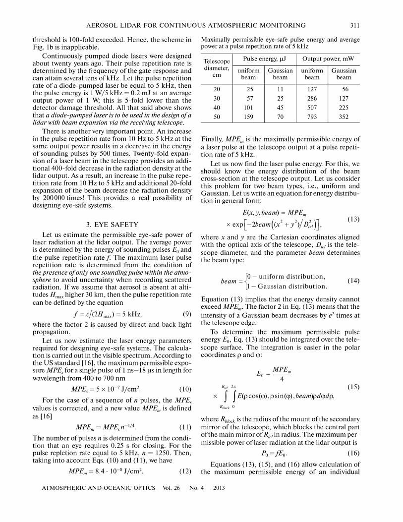
Maximally permissible eye�safe pulse energy and averagepower at a pulse repetition rate of 5 kHz

Telescope diameter,

cm

Pulse energy, µJ Output power, mW

uniform beam

Gaussian beam

uniform beam

Gaussian beam

20 25 11 127 56

30 57 25 286 127

40 101 45 507 225

50 159 70 793 352

312


RAZENKOV

pulse E0 and the average power P0 at the system output.Data for telescopes of 20, 30, 40, and 50 cm in diame�ter for both beam types are tabulated. The block radiusRblock was set equal to 20% of the telescope radius Rtel.

The pulse energy of a Gaussian beam is 45 μJ, andthe average output power is 225 mW for a telescope of40 cm in diameter.

4. BLOCK DIAGRAM OF THE LIDAR

Let us consider a simplified block diagram of aHSRL in Fig. 2.

The lidar consists of three main parts: transmitting,receiving, and calibrating. Let us note that we meaninstrumental calibration, which should not be con�fused with the calibration by molecular scattering. Theinstrumental calibration includes continuous controlof some parameters (e.g., laser frequency) and peri�odic procedures (e.g., frequency scanning to deter�mine the channel bandwidth). The frequency of laserradiation should coincide with the filter absorptionmaximum in the molecular channel for effectiveelimination of aerosol signals. Below we considerfeatures of the laser design and radiation control. Aninterferometer is required to calibrate the frequencyaxis during scanning. Let us note that an interferom�eter design on the basis of single�mode fibers showsgood results [17].

Let us consider the transmitter. The transmittingpart crosses the receiving one, as they have a commontelescope. The transmitter consists of a laser and twobeam expanders, i.e., lens and mirror collimators. Thereceiving telescope is used as the mirror collimator. Wesuggest that the telescope should be just the collimator,i.e., afocal. This scheme has some advantages: it is eas�ily adjustable, and there is no need to focus laser

beams. Mersenne or Dall–Kirkham schemes can bechosen as the afocal telescope [14]. In addition to thetelescope, a TR switch, which diverts lidar returns, iscommon for the transmitter and receiver.

Along with the telescope and the TR switch, thereceiver includes four receiving channels. Let us notethat all the incoming radiation passes through a com�mon field�of�view former, which consists of a focusinglens and an aperture. Then, the beam is collimated anddirected to filters, which cut off the sky background.Systems that used an interference filter along with aFabry–Perot interferometer have a good reputation.In lidars of the University of Wisconsin, the transmis�sion half�width of the Fabry–Perot interferometer is0.008 nm, and that of the interference filter, 0.35 nm[18]. An analyzer is mounted after the filter; it is apolarization element that divides radiation with mutu�ally normal polarizations.

The cross�polarization channel records a signalwith the polarization turning through 90° relative tothe laser radiation polarization. The cross�channel isrequired for measuring the depolarization factor [7].A copolarized signal is divided into three unequalparts so that signals in the molecular and main totalchannel are close in value in conditions of clear air.The molecular channel consists of a filter and a detec�tor; 80% of the flux is directed to it, 19.8% is directedto the main total channel, and 0.2%, to the additionalchannel, which is required in the case of dense cloudsand, hence, signal saturation in the main total chan�nel. Let us note that all the detectors operate in thephoton count mode.

5. TELESCOPE

Let us answer the question, what size the telescopedo we need? One may think that the larger the tele�

TRANSMITTER

RE

CE

IVE

R

Laser

Frequency

Interferometer

Spectrum control

Collimator

Molecular

Iodine filter

Total

TR switch

Field�of�view

Afocal

Filters

Analyzer

Cross�polarization

control channel (80%)

channel (0.2%)

telescope

channelTotal

channel (19.8%)

CA

LIB

RA

TIO

N

Fig. 2. Simplified block�diagram of the high spectral resolution lidar.

former



scope the better, because more photons can be col�lected. This is not quite so in view of the total systemefficiency, because not all the photons coming to thetelescope reach the photodetector. In addition, the skybackground noise, determining the signal�to�noiseratio, should be considered. To eliminate the noise, thereceiver’s field�of�view ϕ should be reduced; moreover,the stable design of the transceiver allows one to dothis. Then a new question arises, how far can wereduce the field of view ϕ? What restricts it frombelow? We assume that this is atmospheric turbulence.Our experience shows that the field�of�view shouldnot be less than 100 μrad, since this results in a morenoticeable (more than 10%) decrease in the echo sig�nal due to breakdown of the laser beam due to turbu�lence in daytime. In other words, an error of 10% is alimit with which we can agree. This error approxi�mately corresponds to the field�of�view ϕ = 100 μrad.

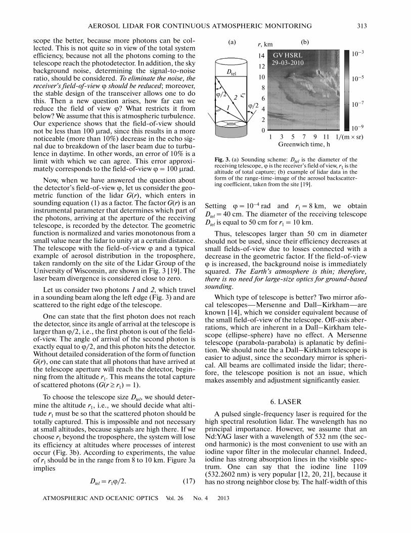
Now, when we have answered the question aboutthe detector’s field�of�view ϕ, let us consider the geo�metric function of the lidar G(r), which enters insounding equation (1) as a factor. The factor G(r) is aninstrumental parameter that determines which part ofthe photons, arriving at the aperture of the receivingtelescope, is recorded by the detector. The geometricfunction is normalized and varies monotonous from asmall value near the lidar to unity at a certain distance.The telescope with the field�of�view ϕ and a typicalexample of aerosol distribution in the troposphere,taken randomly on the site of the Lidar Group of theUniversity of Wisconsin, are shown in Fig. 3 [19]. Thelaser beam divergence is considered close to zero.

Let us consider two photons 1 and 2, which travelin a sounding beam along the left edge (Fig. 3) and arescattered to the right edge of the telescope.

One can state that the first photon does not reachthe detector, since its angle of arrival at the telescope islarger than ϕ/2, i.e., the first photon is out of the field�of�view. The angle of arrival of the second photon isexactly equal to ϕ/2, and this photon hits the detector.Without detailed consideration of the form of functionG(r), one can state that all photons that have arrived atthe telescope aperture will reach the detector, begin�ning from the altitude r1. This means the total captureof scattered photons (G(r ≥ r1) = 1).

To choose the telescope size Dtel, we should deter�mine the altitude r1, i.e., we should decide what alti�tude r1 must be so that the scattered photon should betotally captured. This is impossible and not necessaryat small altitudes, because signals are high there. If wechoose r1 beyond the troposphere, the system will loseits efficiency at altitudes where processes of interestoccur (Fig. 3b). According to experiments, the valueof r1 should be in the range from 8 to 10 km. Figure 3aimplies

Dtel = r1ϕ/2. (17)

Setting ϕ = 10–4 rad and r1 = 8 km, we obtainDtel = 40 cm. The diameter of the receiving telescopeDtel is equal to 50 cm for r1 = 10 km.

Thus, telescopes larger than 50 cm in diametershould not be used, since their efficiency decreases atsmall fields�of�view due to losses connected with adecrease in the geometric factor. If the field�of�viewϕ is increased, the background noise is immediatelysquared. The Earth’s atmosphere is thin; therefore,there is no need for large�size optics for ground�basedsounding.

Which type of telescope is better? Two mirror afo�cal telescopes—Mersenne and Dall–Kirkham—areknown [14], which we consider equivalent because ofthe small field�of�view of the telescope. Off�axis aber�rations, which are inherent in a Dall–Kirkham tele�scope (ellipse�sphere) have no effect. A Mersennetelescope (parabola�parabola) is aplanatic by defini�tion. We should note the a Dall–Kirkham telescope iseasier to adjust, since the secondary mirror is spheri�cal. All beams are collimated inside the lidar; there�fore, the telescope position is not an issue, whichmakes assembly and adjustment significantly easier.

6. LASER

A pulsed single�frequency laser is required for thehigh spectral resolution lidar. The wavelength has noprincipal importance. However, we assume that anNd:YAG laser with a wavelength of 532 nm (the sec�ond harmonic) is the most convenient to use with aniodine vapor filter in the molecular channel. Indeed,iodine has strong absorption lines in the visible spec�trum. One can say that the iodine line 1109(532.2602 nm) is very popular [12, 20, 21], because ithas no strong neighbor close by. The half�width of this

r, km

Dtel

ϕ/2

1

2 r 1

14

12

10

8

6

4

2

01 3 5 7 9 11

10–3GV HSRL29�03�2010

ϕ/2

Greenwich time, h

(a) (b)

10–5

10–7

10–9

1/(m × sr)

Fig. 3. (a) Sounding scheme: Dtel is the diameter of thereceiving telescope, ϕ is the receiver’s field of view, r1 is thealtitude of total capture; (b) example of lidar data in theform of the range�time�image of the aerosol backscatter�ing coefficient, taken from the site [19].

314


RAZENKOV

line is 1.8 GHz. A cell 30 cm long, with iodine vaporsat a temperature of 28°C, at the frequency of line 1109has transmission of no less than 10–4. That is, it sup�presses an aerosol signal in the molecular channeleffectively. An original way of controlling the laser fre�quency was also developed for a laser with a wave�length of 532 nm [22]. Thus, we can say that there ispositive experience, which eliminates the need for“green” Nd lasers. Its main specifications are listedbelow.

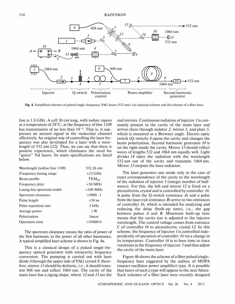
The spectrum clearance means the ratio of power ofthe first harmonic to the power of all other harmonics.A typical simplified laser scheme is shown in Fig. 4a.

This is a classical design of a pulsed single�fre�quency optical generator with intracavity frequencyconversion. The pumping is carried out with laserdiode 6 through the upper side of YAG crystal 8; there�fore, mirror 11 should be dichroic, i.e., it should trans�mit 808 nm and reflect 1064 nm. The cavity of themain laser has a zigzag shape, where 12 and 13 are the

Wavelength (iodine line 1109) 532.26 nm

Frequency tuning range ±15 GHz

Beam profile TEM00

Frequency jitter <30 MHz

Lasing line spectrum width <100 MHz

Spectrum clearance >5000 : 1

Pulse length <50 ns

Pulse repetition rate 5 kHz

Average power 1 W

Polarization linear

Operation time >10000 h

end mirrors. Continuous radiation of injector 1 is con�stantly present in the cavity of the main laser andarrives there through isolator 2, mirror 3, and plate 5,which is mounted at a Brewster angle. Electro�opticswitch (Q�switch) 4 opens the cavity and changes thebeam polarization. Second harmonic generator 10 ison the right inside the cavity. Mirror 13 should reflectwaves of lengths 532 and 1064 nm equally well. Lightdivider 14 takes the radiation with the wavelength532 nm out of the cavity and transmits 1064 nm.Mirror 15 outputs the laser radiation.

The laser generates one mode only in the case ofexact correspondence of the cavity to the wavelengthof the radiation of injector 1 (integer number of half�waves). For this, the left�end mirror 12 is fixed on apiezoelectric crystal and is controlled by controller 16.A pulse from the Q�switch (entrance A) and a pulsefrom the laser exit (entrance B) arrive to two entrancesof controller 16, which is intended for analyzing andreducing the delay (built�up time), i.e., the gapbetween pulses A and B. Minimum built�up timemeans that the cavity size is adjusted to the injectorwavelength. The control voltage comes from entranceC of controller 16 to piezoelectric crystal 12. In thisscheme, the frequency of injector 1 is controlled inde�pendently of operation of controller 16 via a change inits temperature. Controller 16 is to have time to tracevariations in the frequency of injector 1 and thus adjustthe cavity of the main laser.

Figure 4b shows the scheme of a fiber pulsed single�frequency laser suggested by the author, of MOPA(master oscillator power amplifier) type. It is possiblethat lasers of such a type will appear in the near future.Such schemes of a fiber laser were recently designed

808 nm

Injector Q�switch Polarization Second harmonic

1064 nm

1064 nm 808 nm

532 nm

1064 nm

1064 nm

control

532 nm

532 nm

generatorPower amplifier

A B

C

1

2 3

45

6

9

1011

12

13

2

1

3 3 33

547

7

8

8

9

6

14

10

15

16

Fig. 4. Simplified schemes of pulsed single�frequency YAG lasers (532 nm): (a) classical scheme and (b) scheme of a fiber laser.



[23, 24]. A semiconductor frequency�tunable narrow�bandwidth distributed feedback laser (DBL) should beused as injector 1 in Fig. 4b. To protect injector 1 fromprobable reflections, isolator 2 is added. Fusion splic�ing joints are marked by 3. Q�switch 4 can be made ofpiezoelectric ceramics.

Piezoelectric fiber compression generates the effectof birefringence, which changes the light polarization[24]. Polarization controller 5 specifies the polariza�tion conditions and should be adjusted along withQ�switch 4. Wavelength division multiplexing 7(WDM) combines the injector radiation (1064 nm)with the pumping radiation (808 nm) from laserdiode 6, which then comes to fiber 8 with double coreand Nd in the middle. Radiation of diode 6 is absorbedby Nd, and then radiation of injector 1 amplifies infiber 8. End 9 of fiber 8 is polished at a Brewster angleto decrease reflection. Nonlinear crystal 10, e.g.,potassium�titanyl�phosphate, converts IR laser radia�tion with the wavelength 1064 nm to 532 nm.

7. OPTICAL SHEME

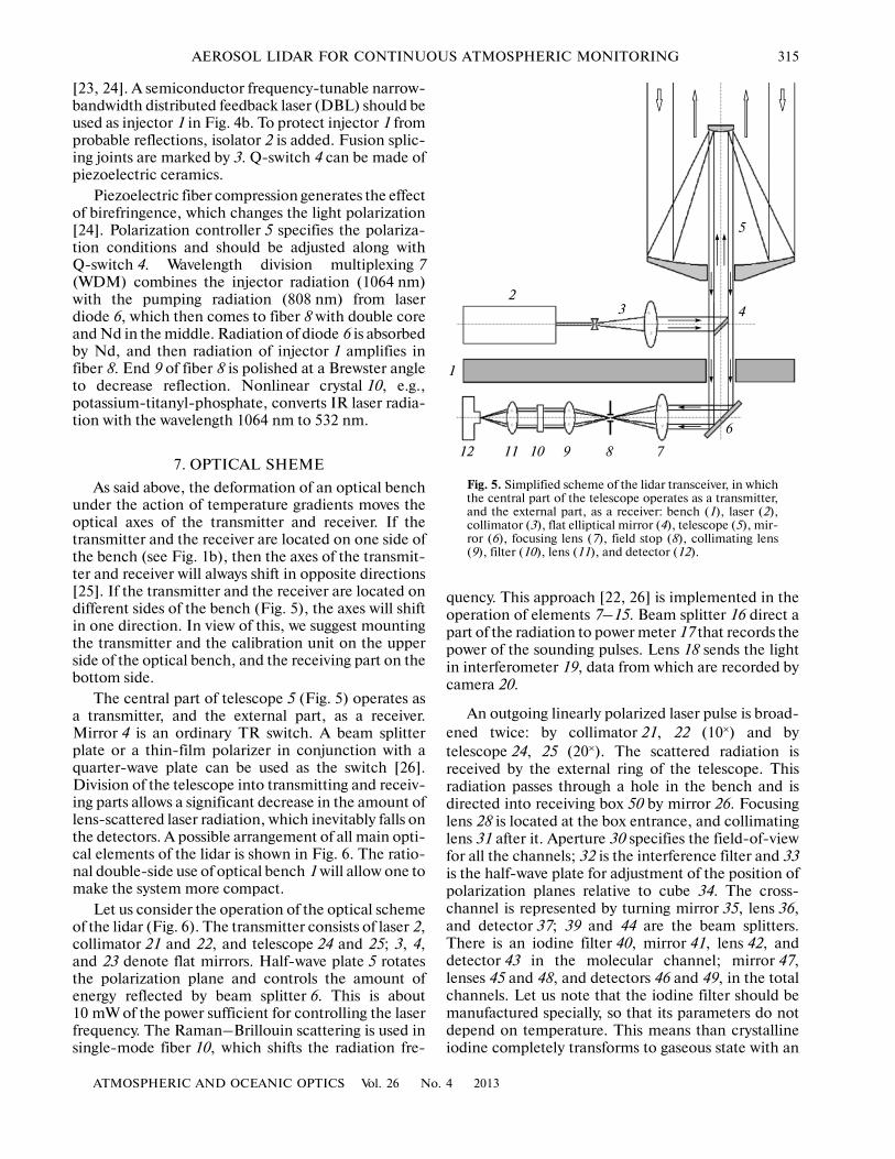
As said above, the deformation of an optical benchunder the action of temperature gradients moves theoptical axes of the transmitter and receiver. If thetransmitter and the receiver are located on one side ofthe bench (see Fig. 1b), then the axes of the transmit�ter and receiver will always shift in opposite directions[25]. If the transmitter and the receiver are located ondifferent sides of the bench (Fig. 5), the axes will shiftin one direction. In view of this, we suggest mountingthe transmitter and the calibration unit on the upperside of the optical bench, and the receiving part on thebottom side.

The central part of telescope 5 (Fig. 5) operates asa transmitter, and the external part, as a receiver.Mirror 4 is an ordinary TR switch. A beam splitterplate or a thin�film polarizer in conjunction with aquarter�wave plate can be used as the switch [26].Division of the telescope into transmitting and receiv�ing parts allows a significant decrease in the amount oflens�scattered laser radiation, which inevitably falls onthe detectors. A possible arrangement of all main opti�cal elements of the lidar is shown in Fig. 6. The ratio�nal double�side use of optical bench 1 will allow one tomake the system more compact.

Let us consider the operation of the optical schemeof the lidar (Fig. 6). The transmitter consists of laser 2,collimator 21 and 22, and telescope 24 and 25; 3, 4,and 23 denote flat mirrors. Half�wave plate 5 rotatesthe polarization plane and controls the amount ofenergy reflected by beam splitter 6. This is about10 mW of the power sufficient for controlling the laserfrequency. The Raman–Brillouin scattering is used insingle�mode fiber 10, which shifts the radiation fre�

quency. This approach [22, 26] is implemented in theoperation of elements 7–15. Beam splitter 16 direct apart of the radiation to power meter 17 that records thepower of the sounding pulses. Lens 18 sends the lightin interferometer 19, data from which are recorded bycamera 20.

An outgoing linearly polarized laser pulse is broad�ened twice: by collimator 21, 22 (10×) and bytelescope 24, 25 (20×). The scattered radiation isreceived by the external ring of the telescope. Thisradiation passes through a hole in the bench and isdirected into receiving box 50 by mirror 26. Focusinglens 28 is located at the box entrance, and collimatinglens 31 after it. Aperture 30 specifies the field�of�viewfor all the channels; 32 is the interference filter and 33is the half�wave plate for adjustment of the position ofpolarization planes relative to cube 34. The cross�channel is represented by turning mirror 35, lens 36,and detector 37; 39 and 44 are the beam splitters.There is an iodine filter 40, mirror 41, lens 42, anddetector 43 in the molecular channel; mirror 47,lenses 45 and 48, and detectors 46 and 49, in the totalchannels. Let us note that the iodine filter should bemanufactured specially, so that its parameters do notdepend on temperature. This means than crystallineiodine completely transforms to gaseous state with an

1

23 4

5

6

789101112

Fig. 5. Simplified scheme of the lidar transceiver, in whichthe central part of the telescope operates as a transmitter,and the external part, as a receiver: bench (1), laser (2),collimator (3), flat elliptical mirror (4), telescope (5), mir�ror (6), focusing lens (7), field stop (8), collimating lens(9), filter (10), lens (11), and detector (12).

316


RAZENKOV

increase in temperature. Such a filter is called starved.We do not consider here the manufacturing technol�ogy of starved iodine filters.

Neutral light filters 27 and 38 are required forinstrumental calibrations, to attenuate the scatteredlight from the laser, which arrives from the transmit�ting channel and is used for frequency calibrationscanning (once per day). Shutter 29 closes all thedetectors. The filters and the shutter are controlled viaa PC. Another one of the background noise filters—aFabry–Perot interferometer—is not shown in thescheme, but it can be added and mounted between

elements 32 and 33. The main specifications of thereceiver are listed below.

Afocal Dall–Kirkham or Mersen telescope 400 mm

Telescope magnification 20×

Field�of�view 100 µrad

Half�width of the interference filter 0.3 nm

Transmission of the interference filter 70%

Half�width of the iodine filter 1.8 GHz

Transmission of the iodine filter (center of line 1109)

10–4

1

23

17 1816

15

1211

9

24

25

87

1314

1019 20

2322

21654

4847

49

44 4546

43

42

5039

37

36

3534

40 41

28

26

27

3833 32 31 30

29

Fig. 6. Optical scheme of the lidar.



8. MODEL ESTIMATES

Equation (2) for a molecular signal can be rewrit�ten for the number of received photons Nm(r) as

(18)

where N0 is the number of photons in a laser pulse, kopt

is the optical path transmission, Δr is the value of a binof the recording system. The average eye�safe laserradiation power P0 is equal to 225 mW for a 400�mmtelescope, according to the table from Part 3; the pulseenergy E0 = 45 μJ. The number of photons in a laserpulse N0 is defined by the division of the energy E0 bythe photon energy and equal to 1.2 × 1014. The effec�tive quantum efficiency of a Perkin Elmer detector is60%.

The profile of the molecular backscattering coeffi�cient βm(r) is calculated on the basis of models for thetemperature and pressure [2, 8]. The geometric factorG(r) is calculated using the author’s model:

(19)

Here r1 is the parameter depending on the size ofthe transceiver; r1 = 10 km for a telescope of 400 mmin diameter, and G(r) ≡ 1 for r > r1. Equation (19) isproportional to ∼r2 at small r. This is caused by thetransceiver design, where the transmission and receiv�ing are carried out via one telescope.

The parameter kopt includes the transmission of theinterference filter (0.5), of the beam splitter plate(0.8), of the iodine filter (0.25), and the total transmis�sion of the optics (0.3). The resulted optical pathtransmission kopt is equal to 0.03.

Let us estimate a relative calculation error of theaerosol backscattering coefficient. Assume that the airis clear, the aerosol scattering signal is approximatelyequal to the molecular scattering signal, and the errorsare totally mutually independent. Then, differentiat�ing Eq. (3), we find the relative error of the aerosolscattering coefficient

(20)

where δNm is the relative signal recording error. Lidarsignals are random values obeying Poisson statistics.The equation for the relative error δNm depends on thenumber of photons accumulated in each bin Nm(r):

(21)

Effective quantum efficiency of Perkin–Elmer SPCM�AQR�12 detectors

60%

Spatial resolution 7.5 m

Temporal resolution 1 s

20( ) ( )( ) ( ),m m opt mN r N k G r A r r r= η Δ β

21

41

2( )( ) .

1 ( )

r rG r

r r=

+

2 ,a mNδβ = δ

1( ) .( )

mm

N rN r

δ =

Equation (18) defines the number of photons receivedin a bin per one laser shot. If the signals are accumu�lated during Δt s, then Eq. (21) takes the form

(22)1( ) ,( )

mm

N rtfN r

δ =Δ

201000.00001

0.0001

(a)

(b)

0.001

0.01

0.1

0.01

1

10

100

1000

Nm(r) δβa(r), %

r, km

1 2 3

4 5

201000.00001

0.0001

0.001

0.01

0.1

0.1

1

10

100

1000

Nm(r) δτ(r), %

r, km

1 2 3

4 5

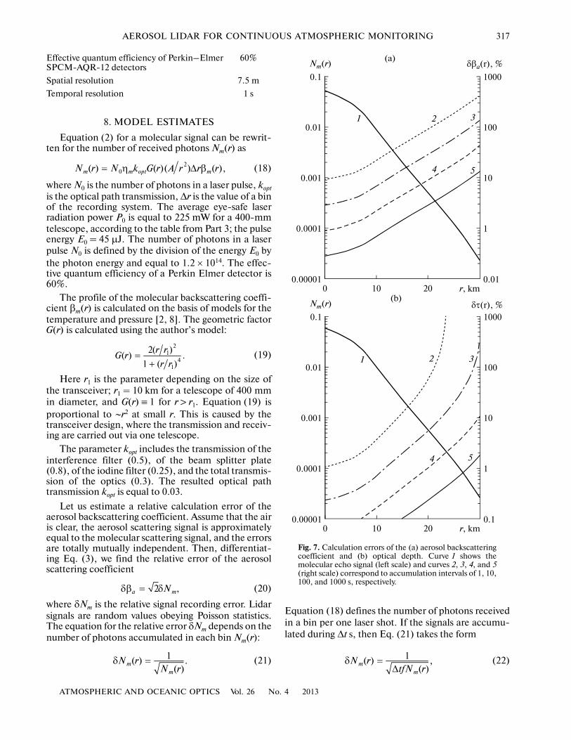
Fig. 7. Calculation errors of the (a) aerosol backscatteringcoefficient and (b) optical depth. Curve 1 shows themolecular echo signal (left scale) and curves 2, 3, 4, and 5(right scale) correspond to accumulation intervals of 1, 10,100, and 1000 s, respectively.

318


RAZENKOV

and the relative error of the aerosol scattering coeffi�cient is written as

(23)

Figure 7a shows the altitude profile of a signal with�out accumulation (curve 1, left scale) calculated byEq. (18) and the relative calculation errors of the aero�sol backscattering coefficient (curves 2–5, right scale)calculated by Eq. (23) for averaging intervals 1, 10,100, and 1000 s.

If 10% accuracy is appropriate, then the maximumsouding altitude is 3.5, 13, 21, and 29 km, respectively,for the above averaging intervals. In practice, an accu�mulation period of 1 min seems optimal.

2( ) .( )

am

rtfN r

δβ =Δ

The equation for the relative error of the opticaldepth τ(r) is derived from differentiation of Eq. (4):

(24)

Equation (24) takes into account only signalrecording errors and corresponds to a high air trans�parency. Figure 7b shows the altitude profile of a signalwithout accumulation (curve 1, left scale) calculatedby Eq. (18) and the relative calculation errors of opti�cal depth (curves 2–5, right scale) calculated byEq. (24) for averaging intervals 1, 10, 100, and 1000 s.The error is equal to 10% in the end of a path 30 kmlong for a 100�s averaging interval and at a distance of23 km for a 10�s averaging interval.

CONCLUSIONS

We have considered a prototype of a high spectralresolution lidar, which satisfies the following criteria ofan up�to�date aerosol lidar. The lidar is to be molecu�lar�scattering calibrated and eye�safe. It is to operatepermanently and unattended; the system design is toprovide on�line remote control for all units. Theapproach considered is aimed at designing a stableopto�mechanical construction, which is to be adjustedonce and operate further without tunning.

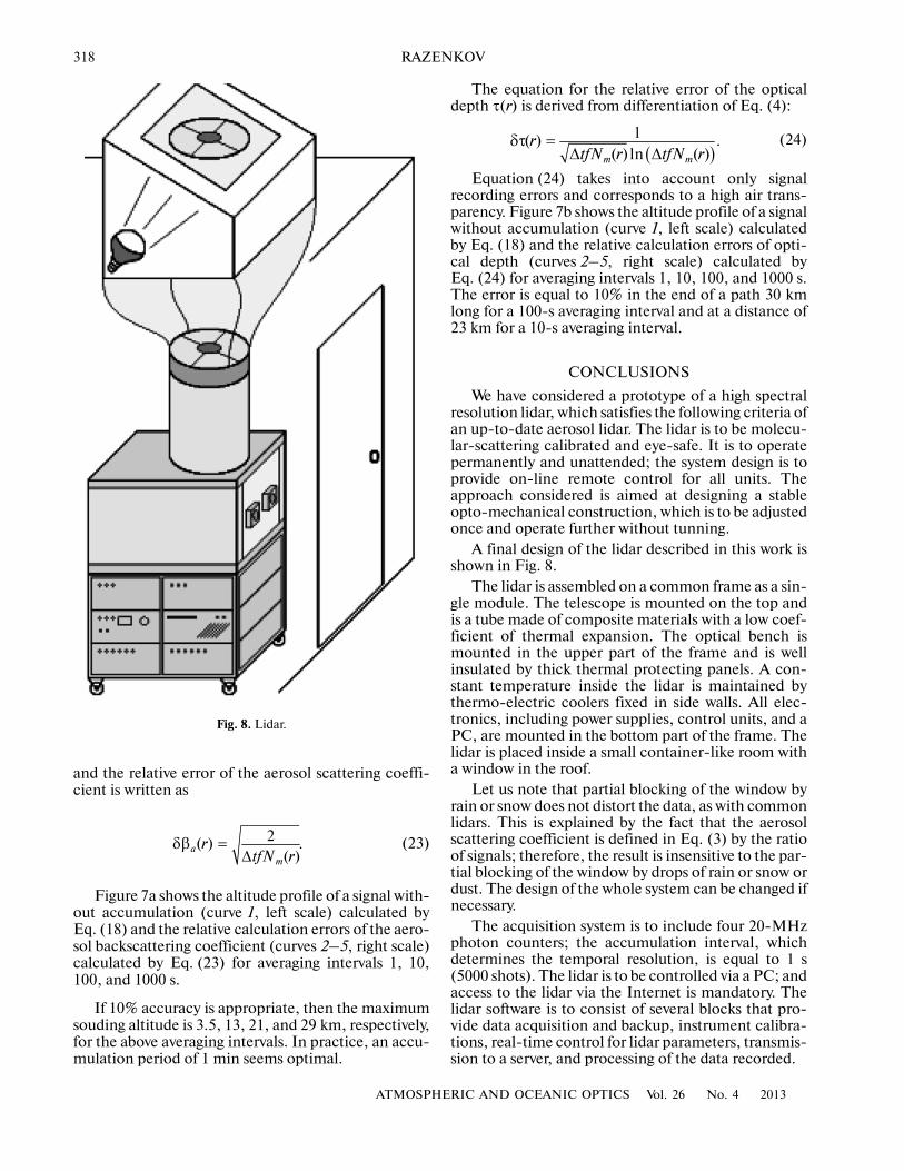
A final design of the lidar described in this work isshown in Fig. 8.

The lidar is assembled on a common frame as a sin�gle module. The telescope is mounted on the top andis a tube made of composite materials with a low coef�ficient of thermal expansion. The optical bench ismounted in the upper part of the frame and is wellinsulated by thick thermal protecting panels. A con�stant temperature inside the lidar is maintained bythermo�electric coolers fixed in side walls. All elec�tronics, including power supplies, control units, and aPC, are mounted in the bottom part of the frame. Thelidar is placed inside a small container�like room witha window in the roof.

Let us note that partial blocking of the window byrain or snow does not distort the data, as with commonlidars. This is explained by the fact that the aerosolscattering coefficient is defined in Eq. (3) by the ratioof signals; therefore, the result is insensitive to the par�tial blocking of the window by drops of rain or snow ordust. The design of the whole system can be changed ifnecessary.

The acquisition system is to include four 20�MHzphoton counters; the accumulation interval, whichdetermines the temporal resolution, is equal to 1 s(5000 shots). The lidar is to be controlled via a PC; andaccess to the lidar via the Internet is mandatory. Thelidar software is to consist of several blocks that pro�vide data acquisition and backup, instrument calibra�tions, real�time control for lidar parameters, transmis�sion to a server, and processing of the data recorded.

( )1( ) .

( ) ln ( )m m

rtfN r tfN r

δτ =Δ Δ

Fig. 8. Lidar.



In the design suggested of a stable laser transceiverfor a high spectral resolution lidar, we used the experi�ence gained during several years in the Lidar Group ofthe University of Wisconsin (Unites States), headed byEdwin W. Eloranta [19, 25–27]. This relates to the cir�cuit of laser frequency stabilization, aerosol signal fil�tration in the molecular channel by an iodine vapor fil�ter, the use of a Fabry–Perot interferometer in thereceiver, etc. The main idea is to design a new�genera�tion calibrated lidar for measuring optical parametersof the atmosphere continuously and correctly.

REFERENCES

1. R. M. Measures, Laser Remote Sensing (Krieger Pub�lishing Company, Florida, 1992).

2. Lidar: Range�Resolved Optical Remote Sensing of theAtmosphere, Ed. by C. Weitkamp (Shpringer, Berlin,2005).

3. J. D. Spinhirne, “Micro Pulse Lidar,” IEEE Trans.Geosci. Remote Sens. 31 (1), 48–55 (1993).

4. S. A. Stewart, E. J. Welton, and T. A. Berkoff, “Solu�tions to Overlap Temperature Sensitivity in Micro PulseLidars,” in Proc. of the 25th Int. Laser Radar Confer�ence, July 5�9, 2010, St. Petersburg, Russia, p. 907–910.

5. http://www.sesi�md.com/miro�pulse�lidar.html

6. V. A. Kovalev and W. E. Eichinger, Elastic Lidar: The�ory, Practice, and Analysis Methods (Wiley�IEEE,2004).

7. Yu. S. Balin, B. V. Kaul’, and G. P. Kokhanenko,“Observations of Specularly Reflective Particles andLayers in Crystal Clouds,” Opt. Atmosf. Okeana 24 (4),293–299 (2011).

8. A. Young, “Rayleigh Scattering,” Appl. Opt. 20, 533–535 (1981).

9. Yu. Arshinov, S. Bobrovnikov, I. Serikov, A. Ansmann,U. Wandinger, D. Althausen, I. Mattis, and D. Müller,“Daytime Operation of a Pure Rotational Raman Lidarby Use of a Fabry�Perot Interferometer,” Appl. Opt. 44(17), 3593–3603 (2005).

10. S. T. Shipley, D. H. Tracy, E. W. Eloranta, J. T. Tauger,J. T. Sroga, F. L. Roesler, and J. A. Weinman, “HighSpectral Resolution Lidar to Measure Optical Scatter�ing Properties of Atmospheric Aerosols. 1. Theory andInstrumentation,” Appl. Opt. 22 (23), 3716–3724(1983).

11. G. Fiocco, G. Beneditti�Michelangeli, K. Maisch�berger, and E. Madonna, “Measurement of Tempera�ture and Aerosol to Molecule Ratio in the Troposphereby Optical Radar,” Nature Phys. Sci. 229, 78–79(1971).

12. P. Piironen and E. W. Eloranta, “Demonstration of aHigh�Spectral�Resolution Lidar Based on an IodineAbsorption Filter,” Opt. Lett. 19 (3), 234–236 (1994).

13. J. Harms, W. Lahmann, and C. Weitkamp, “Geometri�cal Compression of Lidar Return Signals,” Appl.Opt. 17 (7), 1131–1135 (1978).

14. D. D. Maksutov, Astronomical Optics (Nauka, Lenin�grad, 1979), 2nd ed. [in Russian].

15. J. W. Hair, C. A. Hostetler, A. L. Cook, D. B. Harper,R. A. Ferrare, T. L. Mack, Wayne Welch, L. R. Izquierdo,and F. E. Hovis, “Airborne High Spectral ResolutionLidar for Profiling Aerosol Optical Properties,” Appl.Opt. 47 (36), 6734–6753 (2008).

16. American National Standard Z136. 1�1993.17. Z. G. Wang, Ph.D. Dissertation (Virginia Polytechnic

Institute and State University, Blacksburg, 1996).18. I. A. Razenkov, E. W. Eloranta, J. P. Hedrick, R. E. Holz,

R. E. Kuehn, and J. P. Garcia, “A High Spectral Reso�lution Lidar Designed for Unattended Operation in theArctic,” in Proc. of the 21st Int. Laser Radar Conference,July 8–12, 2002, Quebec, Canada, p. 57–60.

19. http://lidar.ssec.wisc.edu20. J. N. Forkey, Ph.D. dissertation (Princeton University,

1996).21. J. W. Hair, L. M. Caldwell, D. A. Krueger, and C.�Y. She,

“High Spectral�Resolution Lidar with Iodine�VaporFilters: Measurement of Atmospheric�State and Aero�sol Profiles,” Appl. Opt. 40 (30), 5280–5294 (2001).

22. E. W. Eloranta and I. A. Razenkov, “Frequency Lock�ing to the Center of a 532 nm Iodine Absorption Lineby Using Stimulated Brillouin Scattering from a Single�Mode Fiber,” Opt. Lett. 31 (5), 598–600 (2006).

23. A. Alvarez�Chavez, H. L. Offerhaus, J. Nilsson,P. W. Turner, W. A. Clarkson, and D. J. Richardson,“High�Energy, High�Power Ytterbium�Doped Q�Switched Fiber Laser,” Opt. Lett. 25 (1), 37–39 (2006).

24. Shi Wei, E. B. Petersen, and D. T. Nguyen, Yao Zhi�dong, Arturo Chavez�Pirson, N. Peyghambarian, andYu. Jirong, “220 µJ Monolithic Single�Frequency Q�Switched Fiber Laser at 2 µm by Using Highly Tm�Doped Germanate Fibers,” Opt. Lett. 36 (18), 3575–3577 (2011).

25. I. A. Razenkov, E. W. Eloranta, and I. I. Razenkov,“Stable Coaxial Lidar Transceiver,” in Proc. of the 25thInt. Laser Radar Conference, July 5–9, 2010, St. Peters�burg, Russia, p. 195–198.

26. I. A. Razenkov, E. W. Eloranta, J. P. Hedrick, andJ. P. Garcia, “Arctic High Spectral Resolution Lidar,”Opt. Atmosf. Okeana 25 (1), 94–102 (2012).

27. I. I. Razenkov, E. W. Eloranta, M. Lawson, andJ. P. Garcia, “Mobile High Spectral Resolution Lidar,”in Proc. of the 26th Int. Laser Radar Conference, June25–29, 2012, Porto Heli, Greece.

Translated by O. Ponomareva

aerosol lidar for continuous atmospheric monitoring

Documents