aeroacoustic analysis of a rod-airfoil flow by means of … · 2017-01-30 · test conﬂguration...

UNCLASSIFIED

Executive summary

UNCLASSIFIED

Nationaal Lucht- en Ruimtevaartlaboratorium

National Aerospace Laboratory NLR

This report is based on a presentation held at 15th AIAA/CEAS Aeroacoustic Conference, Miami, Florida, 11-13 May 2009.

Report no. NLR-TP-2009-440 Author(s) V. Lorenzoni P. Moore F. Scarano M. Tuinstra Report classification UNCLASSIFIED Date 20 August 2009 Knowledge area(s) Aëro-akoestisch en experimenteel aërodynamisch onderzoek Descriptor(s) Rod-Airfoil PIV Sound Acoustic Analogy Curle's Analogy

Aeroacoustic analysis of a rod-airfoil flow by means of time-resolved PIV

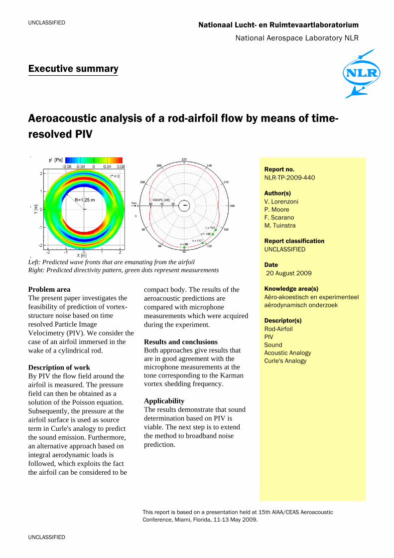
Left: Predicted wave fronts that are emanating from the airfoil Right: Predicted directivity pattern, green dots represent measurements

Problem area The present paper investigates the feasibility of prediction of vortex-structure noise based on time resolved Particle Image Velocimetry (PIV). We consider the case of an airfoil immersed in the wake of a cylindrical rod. Description of work By PIV the flow field around the airfoil is measured. The pressure field can then be obtained as a solution of the Poisson equation. Subsequently, the pressure at the airfoil surface is used as source term in Curle's analogy to predict the sound emission. Furthermore, an alternative approach based on integral aerodynamic loads is followed, which exploits the fact the airfoil can be considered to be

compact body. The results of the aeroacoustic predictions are compared with microphone measurements which were acquired during the experiment. Results and conclusions Both approaches give results that are in good agreement with the microphone measurements at the tone corresponding to the Karman vortex shedding frequency. Applicability The results demonstrate that sound determination based on PIV is viable. The next step is to extend the method to broadband noise prediction.

UNCLASSIFIED

UNCLASSIFIED


Nationaal Lucht- en Ruimtevaartlaboratorium, National Aerospace Laboratory NLR Anthony Fokkerweg 2, 1059 CM Amsterdam, P.O. Box 90502, 1006 BM Amsterdam, The Netherlands Telephone +31 20 511 31 13, Fax +31 20 511 32 10, Web site: www.nlr.nl

Nationaal Lucht- en Ruimtevaartlaboratorium National Aerospace Laboratory NLR

NLR-TP-2009-440


V. Lorenzoni1, P. Moore1, F. Scarano1 and M. Tuinstra

1 TU Delft

This report is based on a presentation held at 15th AIAA/CEAS Aeroacoustic Conference, Miami, Florida, 11-13 May 2009. The contents of this report may be cited on condition that full credit is given to NLR and the authors. This publication has been refereed by the Advisory Committee AEROSPACE VEHICLES. Customer National Aerospace Laboratory NLR Contract number ---- Owner National Aerospace Laboratory NLR + partner(s) Division NLR Aerospace Vehicles Distribution Unlimited Classification of title Unclassified January 2010 Approved by:

Author

Reviewer Managing department

NLR-TP-2009-440

2

Contents

Nomenclature 3 I Introduction 4 II Aeroacoustic model 4 III Experiment 5 IV Acoustic prediction 10 V Conclusion 13 Acknowledgements 14 References 14

NLR-TP-2009-440

3

Aeroacoustic analysis of a rod-airfoil flow by means of

time-resolved PIV

Lorenzoni V.,∗ Moore P.,† Scarano F.‡

Delft University of Technology, Aerospace Engineering Department, Delft, 2629 HS, The Netherlands

Tuinstra M.§

Dutch National Aerospace Laboratory NLR, 8316 PR, Marknesse, The Netherlands

The present study investigates an experimental approach for aeroacoustic prediction ofvortex-structure noise based on time-resolved Particle Image Velocimetry (TR-PIV). Thetest configuration consists of a NACA0012 airfoil immersed in the wake of an cylindricalrod. The velocity field around the airfoil measured by the PIV experiment is used toevaluate the corresponding pressure field as solution of the planar Poisson equation forthe pressure. The resulting pressure evaluated at the airfoil surface constitutes the sourceterm of the implemented Curle’s aeroacoustic analogy. An alternative formulation basedon the integral aerodynamic loads is also followed. The results of the aeroacoustic predic-tion are compared with microphone measurements conducted simultaneously, in terms ofspectra and directivity pattern. The results show a good agreement with the microphonemeasurements for the evaluation of the tonal component corresponding to the frequencyof interaction of the Karman vortices with the airfoil leading edge.

Nomenclature

St Strouhal numberRe Reynolds numbery Acoustic source position [m]x Listener position [m]δij Kronecker deltate Retarded timer Distance between generic surface point and listener positionR Distance between airfoil leading edge and listener positionp0 Atmospheric pressure [Pa]p′ Pressure fluctuation p− p0 [Pa]c0 Speed of sound [m/s]〈f(x, t)〉 Local time averageffluct Local time fluctuation f(x, y, t)− 〈f(x, t)〉rms Root mean square valueSPL Sound pressure level [Pa]OASPL Overall sound pressure level [Pa]C.L. Correlation length [% of span]Tshed Shedding period [s]t∗ Normalized time [t/Tshed]CV Control volume for evaluation of aerodynamic loadsLE Airfoil leading edge

∗Research Assistant, Aerodynamic Section†Researcher, Aerodynamic Section‡Professor, Aerodynamic Section§NLR Researcher, Dutch National Aerospace Laboratory NLR.

1 of 12

American Institute of Aeronautics and Astronautics

15th AIAA/CEAS Aeroacoustics Conference (30th AIAA Aeroacoustics Conference)11 - 13 May 2009, Miami, Florida

AIAA 2009-3298

Copyright © 2009 by the American Institute of Aeronautics and Astronautics, Inc. All rights reserved.

NLR-TP-2009-440

4

I. Introduction

Vortex-structure interaction noise is become of main concern in aeronautics as well as in various in-dustrial environments. Several devices are arranged in such a way that downstream bodies are embedded

in the wake of upstream bodies. This is typically the case of a bank of heat exchanger tubes, rotor statorconfigurations of turbo-engines, ventilating systems and helicopter rotors in case of vortex-blade interaction.The rod-airfoil configuration as test case of combined vortex shedding noise and turbulence-structure inter-action noise was proposed by Jacobs1 as benchmark test configuration of numerical CFD codes (URANS,LES) for broadband noise predictions. Casalino2 applied URANS simulations for the characterization of theflow field on the same configuration and developed an advanced-time numerical code for noise predictionbased on Ffowcs Williams-Hawkings equation. Numerical investigations on the same configuration have beenperformed inside the framework of European Project PROBAND.3 The results obtained by the application ofseveral computational aeroacoustic (CAA) techniques have been compared with experimental measurementsfor the assessment on the broadband noise prediction.

To the knowledge of the authors, the time-resolved PIV technique for quantitative aeroacoustic predictionon the rod-airfoil configuration has not been explored yet. Recent improvements of velocimetry techniquesover the last two decades in terms of spatial and temporal resolution, have opened the possibility of usingexperimental PIV data for aeroacoustic purposes. In particular, the use of time-resolved PIV (TR-PIV)data in aeroacoustics was first proposed by Seiner4,5 in devising a new methodology for jet noise reduction,using a statistical reformulation of Lighthill’s analogy developed by Goldstein.6 Recently Wernet7 preformedTR-PIV experiments at high repetition rate on the shear layer of hot and cold jets for evaluation of the two-point delayed correlation tensor of the velocity. Schroder et al.8 performed simultaneous PIV and acousticmeasurements on the trailing edge of a flat board at high recording rate for detection of the statistical flowfeatures responsible for the noise emission and the evaluation of the source terms of Howe’s formulation9 forthe trailing edge emission. Henning10 et al. have recently performed PIV experiment and simultaneous mi-crophone measurements on a circular cylinder and inside a leading edge slat to calculate the cross-correlationbetween the velocity/vorticity field and the acoustic pressure, for statistical detection of the flow structuresresponsible for the noise emission. A different approach for PIV based aeroacoustic predictions was followedby Schram11 analyzing the vortex pairing noise due to acoustically driven instabilities in the shear layer ofa subsonic jet. In this case phase-locking of the jet instability allowed for the phase-resolved description ofthe vortex pairing. The evaluation of the aeroacoustic sources was obtained by a conservative formulationof Vortex Sound Theory12,13 for homentropic, low Mach number axisymmetrical free flows. The robustnessof the integral formulation based on conservation of the flow invariants, provided a good agreement of thenoise prediction obtained by PIV data with respect to analytical models.

The mentioned studies were all based on the kinematic properties of the flows with no direct attempttoward the determination of the instantaneous pressure spatial distribution. In this work the acoustic com-putation hinges on the implementation of Curle’s aeroaocustic analogy in a distributed and an integralformulation. Both the approaches require the knowledge of the unsteady pressure for evaluation of theacoustic sources. The pressure field is calculated by numerical integration of the pressure gradient directlyobtained from the momentum conservation law. A similar approach has been lately applied by Haigermoser14

to a cavity flow using planar TR-PIV in a water flow experiment in combination with a pressure reconstruc-tion algorithm and Curle’s analogy. The reliability of the acoustic prediction based on such a method stillneeded to be tested in terms of magnitude of the spectra by comparison with microphone measurements.The scope of the present work is to quantitatively demonstrate, within the technical limits of this specificexperiment, the feasibility of using time-resolved PIV experimental data for the aeroacoustic noise predictionin vortex-structure-interaction problems.

II. Aeroacoustic model

An extension to Lighthill’s aeroacoustic analogy15 to account for the presence of solid bodies inside theflow domain, was developed by Curle.16 The analytical formulation of Curle’s analogy for low Mach numberflows and compact geometries can be rewritten as

p′(x, t) = − xj

4πc0|x|∂

∂t

∫

∂Vy

p′δij

r

∣∣∣t=te

nidS, (1)

2 of 12


NLR-TP-2009-440

5

where the quantity p′ = p− p0 indicates the pressure fluctuation with respect to the atmospheric referencepressure p0. The quantity on the left hand side represents the propagating acoustic pressure while p′ insidethe integral indicates the pressure fluctuation at the body surface induced by the flow dynamics, which isidentified as the source of noise. The quadrupolar term and the viscous dipoles have been neglected becauseof the low Mach number and relatively high Reynolds number of the flow and the acoustic compactness ofthe airfoil.17 The subscript t = te indicates that the pressure fluctuations at the surface have to be evaluatedat the retarded time te = t− r

c0.

An alternative approach for noise prediction in case of compact geometries is based on the evaluationof the time variations of the integral aerodynamic loads acting on the immersed body (Gutin’s principle6).For bodies small compared to the acoustic wavelength it is possible to neglect the retarded time variationsbetween different points on the integration surface. The surface integral of the pressure in equation (1) thencorresponds to the instantaneous lift and drag forces acting on the airfoil section, which have been calculatedby integrating the momentum equation on a control volume (surface) surrounding the airfoil, following theapproach reported by Kurtulus et al.18

The instantaneous pressure field needed for the evaluation of the source terms in both the analogy formu-lations is calculated by exploiting the Planar Pressure Imaging (PPI) technique.19 The pressure gradient ofthe Navier-Stokes equations are obtained from TR-PIV data using the definition of substantial accelerationdisregarding the viscous contribution, following the method adopted by Liu and Katz.20 Application of thedivergence operator to the planar components of pressure gradient leads to the 2D Poisson equation for thepressure

∇2p = −ρ

(∂

∂x

Du

Dt+

∂

∂y

Dv

Dt

). (2)

Equation (2) has been solved using a numerical algorithm reported by de Kat et al.,21 in the assumption ofincompressible flow. Validation of the method using 3D flow data is currently being investigated.

III. Experiment

III.A. Experimental setup

Combined PIV and acoustic experiments were carried out in the small anechoic wind tunnel (KAT) of theDutch “National Aerospace Laboratories” NLR. The anechoic chamber dimension is 5.5 x 5.5 x 2.5 m3 andit is covered with 0.5 m long foam wedges, yielding 99 % acoustic absorption above 500 Hz. The wind tunnelhas an open test section with exit dimensions of 0.51 x 0.38 m2. A cylindrical rod of 6 mm diameter wasvertically mounted 22 cm downstream of the wind tunnel exit. A NACA0012 Plexiglas airfoil, with a chordof 10 cm, was vertically placed in the wake of the rod at zero incidence. The rod and airfoil were placed ata relative distance of 10.2 cm. The configuration was examined for a nominal free-stream velocity of 15 m/swith incoming turbulence level of 0.5% at the centerline.

3 of 12


NLR-TP-2009-440

6

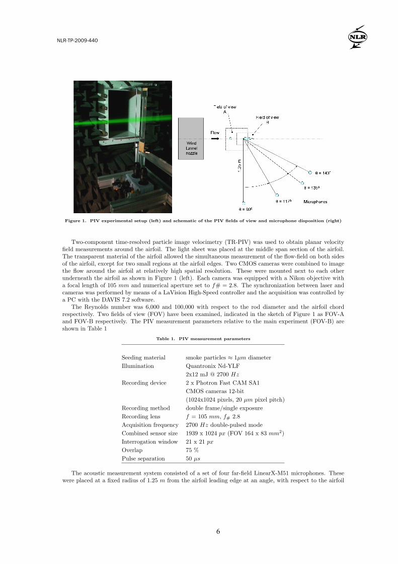
Figure 1. PIV experimental setup (left) and schematic of the PIV fields of view and microphone disposition (right)

Two-component time-resolved particle image velocimetry (TR-PIV) was used to obtain planar velocityfield measurements around the airfoil. The light sheet was placed at the middle span section of the airfoil.The transparent material of the airfoil allowed the simultaneous measurement of the flow-field on both sidesof the airfoil, except for two small regions at the airfoil edges. Two CMOS cameras were combined to imagethe flow around the airfoil at relatively high spatial resolution. These were mounted next to each otherunderneath the airfoil as shown in Figure 1 (left). Each camera was equipped with a Nikon objective witha focal length of 105 mm and numerical aperture set to f# = 2.8. The synchronization between laser andcameras was performed by means of a LaVision High-Speed controller and the acquisition was controlled bya PC with the DAVIS 7.2 software.

The Reynolds number was 6,000 and 100,000 with respect to the rod diameter and the airfoil chordrespectively. Two fields of view (FOV) have been examined, indicated in the sketch of Figure 1 as FOV-Aand FOV-B respectively. The PIV measurement parameters relative to the main experiment (FOV-B) areshown in Table 1

Table 1. PIV measurement parameters

Seeding material smoke particles ≈ 1µm diameterIllumination Quantronix Nd-YLF

2x12 mJ @ 2700 Hz

Recording device 2 x Photron Fast CAM SA1CMOS cameras 12-bit(1024x1024 pixels, 20 µm pixel pitch)

Recording method double frame/single exposureRecording lens f = 105 mm, f# 2.8Acquisition frequency 2700 Hz double-pulsed modeCombined sensor size 1939 x 1024 px (FOV 164 x 83 mm2)Interrogation window 21 x 21 px

Overlap 75 %Pulse separation 50 µs

The acoustic measurement system consisted of a set of four far-field LinearX-M51 microphones. Thesewere placed at a fixed radius of 1.25 m from the airfoil leading edge at an angle, with respect to the airfoil

4 of 12


NLR-TP-2009-440

7

chord of 90◦, 117◦, 135◦, 143◦ as shown in the sketch of Figure 1 (right), at the hight of the airfoil midspan.The microphone recordings were taken simultaneously with the PIV measurements. Table 2 summarizes thecharacteristics of the acoustic measurement system.

Table 2. Acoustic measurement characteristics

Number of far-field microphones 4Angular positions 90◦,117◦,135◦,143◦

Distance from the airfoil 1.25 m

Microphone type LinearX-M51, omnidirectionalpressure microphone

Acquisition system GBM-ViperSample frequency 51.2 kHz

Measuring time 20 s

Frequency resolution 12.5 Hz

III.B. Planar PIV measurements

An overview of the Karman vortex street behind the rod and the interaction of vortical structures with theairfoil LE is provided by FOV-A (Figure 2-left). The detailed visualization of the flow around the entireairfoil is possible in FOV-B, which is needed for evaluation of whole aeroacoustic source. The velocityfield from the PIV recordings was evaluated using the Window Deformation Iterative Multigrid algorithm(WIDIM) developed by Scarano and Riethmuller.22 The spatial resolution of the velocity field correspondedto 1.1 vector/mm (1.1 % chord) for FOV-A and 2.4 vectors/mm (0.4 % chord) for FOV-B. The maximumoperational frequency of the PIV acquisition system at full frame resolution was limited to 2,700 Hz, whichdetermined a time resolution of the velocity field of approximately 5 samples/shedding period.

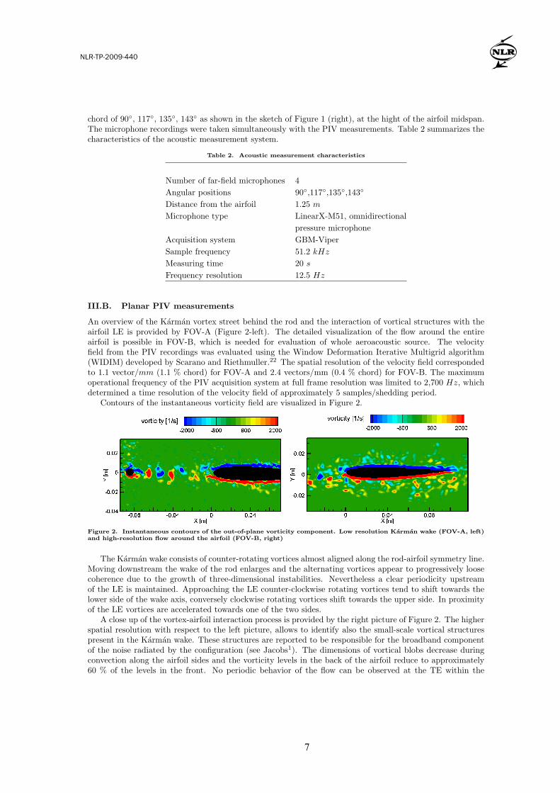
Contours of the instantaneous vorticity field are visualized in Figure 2.

Figure 2. Instantaneous contours of the out-of-plane vorticity component. Low resolution Karman wake (FOV-A, left)and high-resolution flow around the airfoil (FOV-B, right)

The Karman wake consists of counter-rotating vortices almost aligned along the rod-airfoil symmetry line.Moving downstream the wake of the rod enlarges and the alternating vortices appear to progressively loosecoherence due to the growth of three-dimensional instabilities. Nevertheless a clear periodicity upstreamof the LE is maintained. Approaching the LE counter-clockwise rotating vortices tend to shift towards thelower side of the wake axis, conversely clockwise rotating vortices shift towards the upper side. In proximityof the LE vortices are accelerated towards one of the two sides.

A close up of the vortex-airfoil interaction process is provided by the right picture of Figure 2. The higherspatial resolution with respect to the left picture, allows to identify also the small-scale vortical structurespresent in the Karman wake. These structures are reported to be responsible for the broadband componentof the noise radiated by the configuration (see Jacobs1). The dimensions of vortical blobs decrease duringconvection along the airfoil sides and the vorticity levels in the back of the airfoil reduce to approximately60 % of the levels in the front. No periodic behavior of the flow can be observed at the TE within the

5 of 12


NLR-TP-2009-440

8

present measurements. Moreover, the well known laminar separation phenomenon occurring around thisspecific airfoil which leads to TE noise (see Roger23,24), appears to be inhibited by the high turbulence levelof the rod wake where the airfoil is immersed. The large red and blue stripes around the airfoil are due tosaturation of the vorticity levels, which was needed for the visualization of the vortical structures surroundingthe airfoil. The physical boundary layer on the airfoil cannot be captured with the present measurementresolution and the thickness of these stripes should not be taken as an indication of the boundary layer.

III.C. Instantaneous pressure distribution

The pressure field around the airfoil was calculated as solution of the 2D incompressible Poisson equationfor the pressure (equation (2)), using an algorithm developed by de Kat21 based on a second order centraldifference scheme. Dirichlet boundary conditions are taken in the irrotational flow region away from theturbulent wake and are derived from the steady Bernoulli relation. The pressure gradient provided by thePIV measurement, is used as Neumann boundary condition in the rotational parts of the flow boundariesand on the airfoil surface.

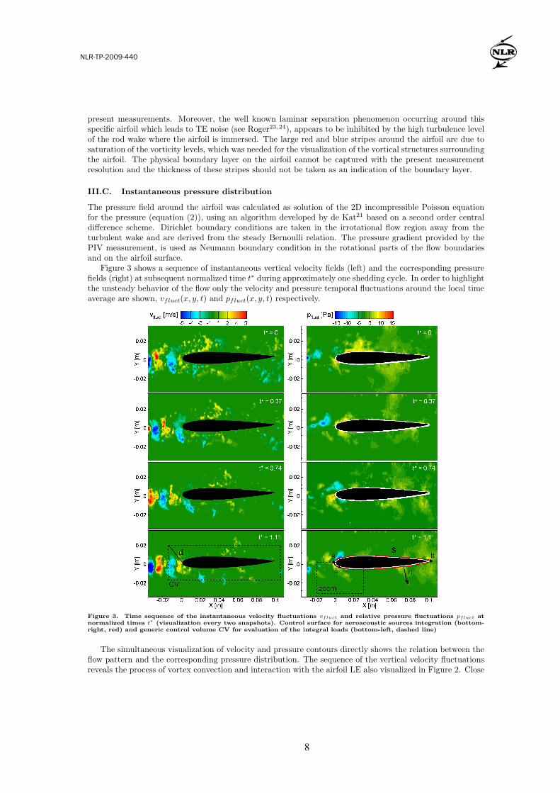
Figure 3 shows a sequence of instantaneous vertical velocity fields (left) and the corresponding pressurefields (right) at subsequent normalized time t∗ during approximately one shedding cycle. In order to highlightthe unsteady behavior of the flow only the velocity and pressure temporal fluctuations around the local timeaverage are shown, vfluct(x, y, t) and pfluct(x, y, t) respectively.

Figure 3. Time sequence of the instantaneous velocity fluctuations vfluct and relative pressure fluctuations pfluct atnormalized times t∗ (visualization every two snapshots). Control surface for aeroacoustic sources integration (bottom-right, red) and generic control volume CV for evaluation of the integral loads (bottom-left, dashed line)

The simultaneous visualization of velocity and pressure contours directly shows the relation between theflow pattern and the corresponding pressure distribution. The sequence of the vertical velocity fluctuationsreveals the process of vortex convection and interaction with the airfoil LE also visualized in Figure 2. Close

6 of 12


NLR-TP-2009-440

9

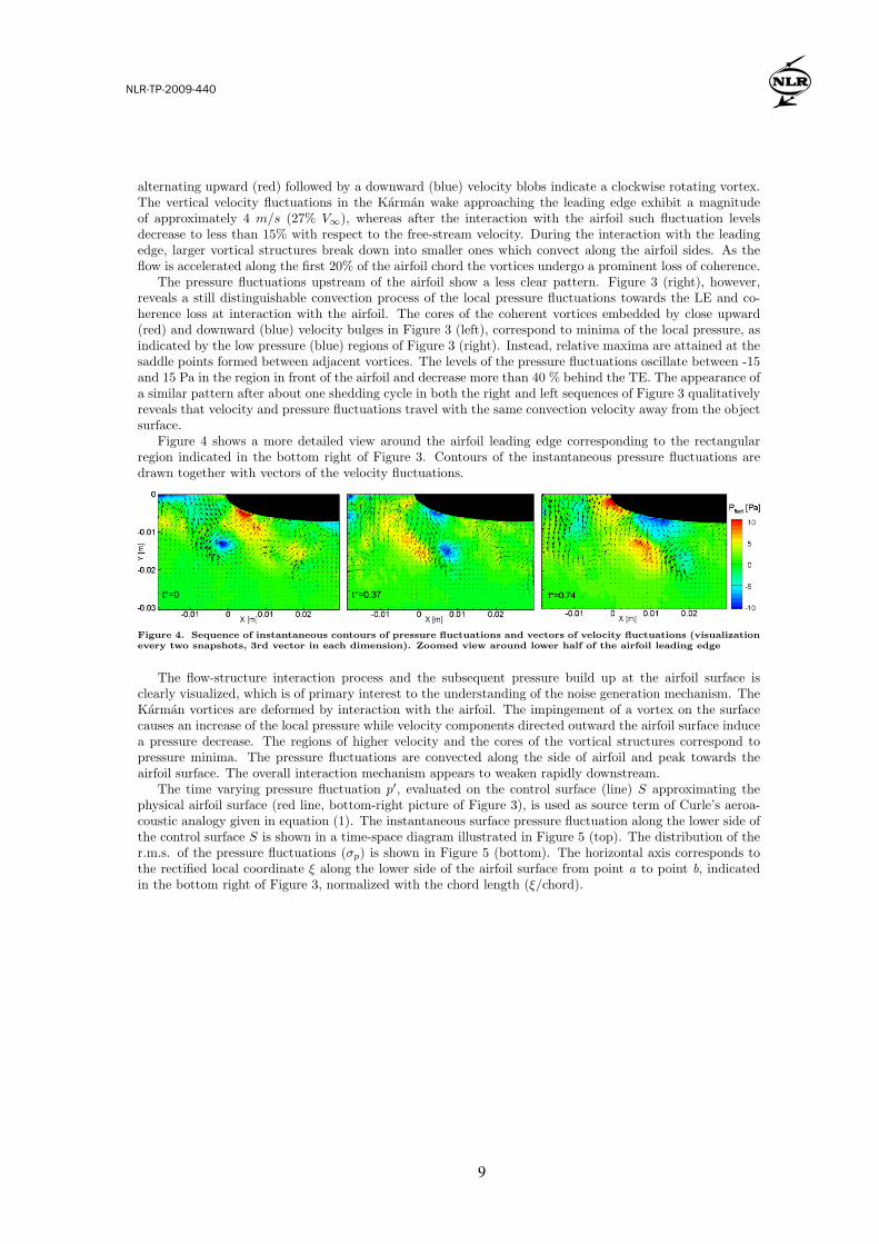
alternating upward (red) followed by a downward (blue) velocity blobs indicate a clockwise rotating vortex.The vertical velocity fluctuations in the Karman wake approaching the leading edge exhibit a magnitudeof approximately 4 m/s (27% V∞), whereas after the interaction with the airfoil such fluctuation levelsdecrease to less than 15% with respect to the free-stream velocity. During the interaction with the leadingedge, larger vortical structures break down into smaller ones which convect along the airfoil sides. As theflow is accelerated along the first 20% of the airfoil chord the vortices undergo a prominent loss of coherence.

The pressure fluctuations upstream of the airfoil show a less clear pattern. Figure 3 (right), however,reveals a still distinguishable convection process of the local pressure fluctuations towards the LE and co-herence loss at interaction with the airfoil. The cores of the coherent vortices embedded by close upward(red) and downward (blue) velocity bulges in Figure 3 (left), correspond to minima of the local pressure, asindicated by the low pressure (blue) regions of Figure 3 (right). Instead, relative maxima are attained at thesaddle points formed between adjacent vortices. The levels of the pressure fluctuations oscillate between -15and 15 Pa in the region in front of the airfoil and decrease more than 40 % behind the TE. The appearance ofa similar pattern after about one shedding cycle in both the right and left sequences of Figure 3 qualitativelyreveals that velocity and pressure fluctuations travel with the same convection velocity away from the objectsurface.

Figure 4 shows a more detailed view around the airfoil leading edge corresponding to the rectangularregion indicated in the bottom right of Figure 3. Contours of the instantaneous pressure fluctuations aredrawn together with vectors of the velocity fluctuations.

Figure 4. Sequence of instantaneous contours of pressure fluctuations and vectors of velocity fluctuations (visualizationevery two snapshots, 3rd vector in each dimension). Zoomed view around lower half of the airfoil leading edge

The flow-structure interaction process and the subsequent pressure build up at the airfoil surface isclearly visualized, which is of primary interest to the understanding of the noise generation mechanism. TheKarman vortices are deformed by interaction with the airfoil. The impingement of a vortex on the surfacecauses an increase of the local pressure while velocity components directed outward the airfoil surface inducea pressure decrease. The regions of higher velocity and the cores of the vortical structures correspond topressure minima. The pressure fluctuations are convected along the side of airfoil and peak towards theairfoil surface. The overall interaction mechanism appears to weaken rapidly downstream.

The time varying pressure fluctuation p′, evaluated on the control surface (line) S approximating thephysical airfoil surface (red line, bottom-right picture of Figure 3), is used as source term of Curle’s aeroa-coustic analogy given in equation (1). The instantaneous surface pressure fluctuation along the lower side ofthe control surface S is shown in a time-space diagram illustrated in Figure 5 (top). The distribution of ther.m.s. of the pressure fluctuations (σp) is shown in Figure 5 (bottom). The horizontal axis corresponds tothe rectified local coordinate ξ along the lower side of the airfoil surface from point a to point b, indicatedin the bottom right of Figure 3, normalized with the chord length (ξ/chord).

7 of 12


NLR-TP-2009-440

10

Figure 5. Time evolution of the pressure fluctuations (top) and r.m.s. value of the pressure (bottom) on a rectifiedcoordinate along the lower side of integration surface S (from a to b).

The vertical axis in the top figure refers to a generic observation time normalized with the sheddingperiod. The diagonal stripes are representative of convection of the pressure fluctuation along the lowerside of the control surface. The inclination of the diagonal lines with respect to the vertical axis indicatesa convection velocity of about 12 m/s. These stripes are spaced time-wise by one shedding cycle. Thediscontinuous appearance of the stripes is ascribed to uncertainty of the velocity measurement specificallyat the solid surface. The r.m.s. of the pressure fluctuations in the bottom plot of Figure 5, calculated over200 cycles along the same coordinate between point a and point b, gives an indication of the average spatialdistribution of the fluctuation magnitude along the control surface S. The region of highest fluctuations islocalized in the first 20 % of the airfoil chord. The intensity of fluctuations drops to less than 50% the peakvalue at half the chord. It is known that aerodynamic sound generation is caused by flow unsteadiness.15

This suggests that the LE region is that mostly responsible for the radiation of acoustic noise in the rod-airfoilconfiguration, confirming the previous results obtained by Jacobs.1

IV. Acoustic prediction

The noise emitted by the airfoil was calculated as solution of equation (1) and its corresponding integralformulation, using a trapezoidal integration method for the surface integral and a forward difference schemefor time derivatives. The PIV experiment and the PPI reconstruction method used for the evaluation of theaeroacoustic sources, provided time-resolved 2D data relative to the midspan airfoil section. The 3D natureof the airfoil emission and the possible cancellation of acoustic sources along the span are accounted for byassuming that an equal in-phase emission occurs along a section of the span corresponding to a fractionof the physical span length. PIV measurements were performed in the spanwise direction on a window

8 of 12


NLR-TP-2009-440

11

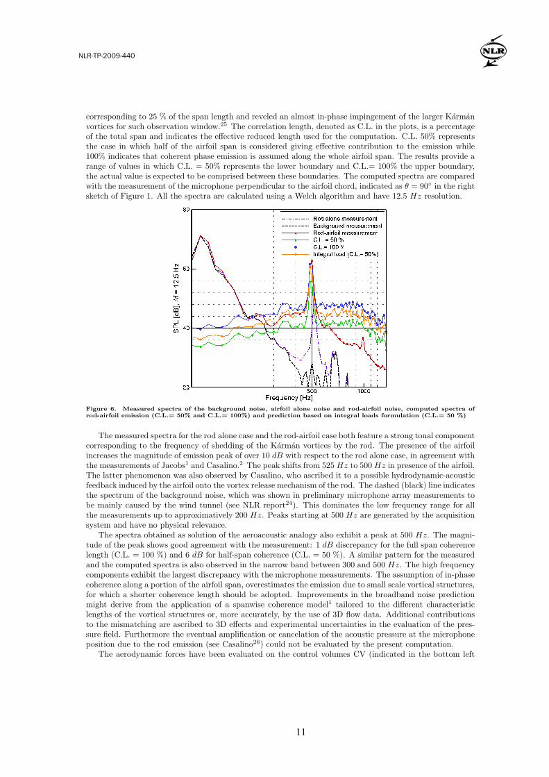
corresponding to 25 % of the span length and reveled an almost in-phase impingement of the larger Karmanvortices for such observation window.25 The correlation length, denoted as C.L. in the plots, is a percentageof the total span and indicates the effective reduced length used for the computation. C.L. 50% representsthe case in which half of the airfoil span is considered giving effective contribution to the emission while100% indicates that coherent phase emission is assumed along the whole airfoil span. The results provide arange of values in which C.L. = 50% represents the lower boundary and C.L.= 100% the upper boundary,the actual value is expected to be comprised between these boundaries. The computed spectra are comparedwith the measurement of the microphone perpendicular to the airfoil chord, indicated as θ = 90◦ in the rightsketch of Figure 1. All the spectra are calculated using a Welch algorithm and have 12.5 Hz resolution.

Figure 6. Measured spectra of the background noise, airfoil alone noise and rod-airfoil noise, computed spectra ofrod-airfoil emission (C.L.= 50% and C.L.= 100%) and prediction based on integral loads formulation (C.L.= 50 %)

The measured spectra for the rod alone case and the rod-airfoil case both feature a strong tonal componentcorresponding to the frequency of shedding of the Karman vortices by the rod. The presence of the airfoilincreases the magnitude of emission peak of over 10 dB with respect to the rod alone case, in agreement withthe measurements of Jacobs1 and Casalino.2 The peak shifts from 525 Hz to 500 Hz in presence of the airfoil.The latter phenomenon was also observed by Casalino, who ascribed it to a possible hydrodynamic-acousticfeedback induced by the airfoil onto the vortex release mechanism of the rod. The dashed (black) line indicatesthe spectrum of the background noise, which was shown in preliminary microphone array measurements tobe mainly caused by the wind tunnel (see NLR report24). This dominates the low frequency range for allthe measurements up to approximatively 200 Hz. Peaks starting at 500 Hz are generated by the acquisitionsystem and have no physical relevance.

The spectra obtained as solution of the aeroacoustic analogy also exhibit a peak at 500 Hz. The magni-tude of the peak shows good agreement with the measurement: 1 dB discrepancy for the full span coherencelength (C.L. = 100 %) and 6 dB for half-span coherence (C.L. = 50 %). A similar pattern for the measuredand the computed spectra is also observed in the narrow band between 300 and 500 Hz. The high frequencycomponents exhibit the largest discrepancy with the microphone measurements. The assumption of in-phasecoherence along a portion of the airfoil span, overestimates the emission due to small scale vortical structures,for which a shorter coherence length should be adopted. Improvements in the broadband noise predictionmight derive from the application of a spanwise coherence model1 tailored to the different characteristiclengths of the vortical structures or, more accurately, by the use of 3D flow data. Additional contributionsto the mismatching are ascribed to 3D effects and experimental uncertainties in the evaluation of the pres-sure field. Furthermore the eventual amplification or cancelation of the acoustic pressure at the microphoneposition due to the rod emission (see Casalino26) could not be evaluated by the present computation.

The aerodynamic forces have been evaluated on the control volumes CV (indicated in the bottom left

9 of 12


NLR-TP-2009-440

12

picture of Figure 3) at a distance from the LE normalized with the airfoil chord (d/chord) correspondingto 0.2 and aspect ratio of 5. The spectrum calculated with the integral formulation (triangle-label, orangeline) shows a similar trend with respect to the distributed formulation. For the same correlation length(C.L. = 50 %) the integral approach exhibits overall magnitude levels of about 5 dB higher. The reasonfor this is currently ascribed to an overestimation of the loads calculated with control volume integration.Assessment on the accuracy of the loads determination method for the rod-airfoil configuration requiresfurther analysis. From an experimental point of view this method offers the advantage of avoiding the directpressure determination at the airfoil surface (see van Oudheusden19).

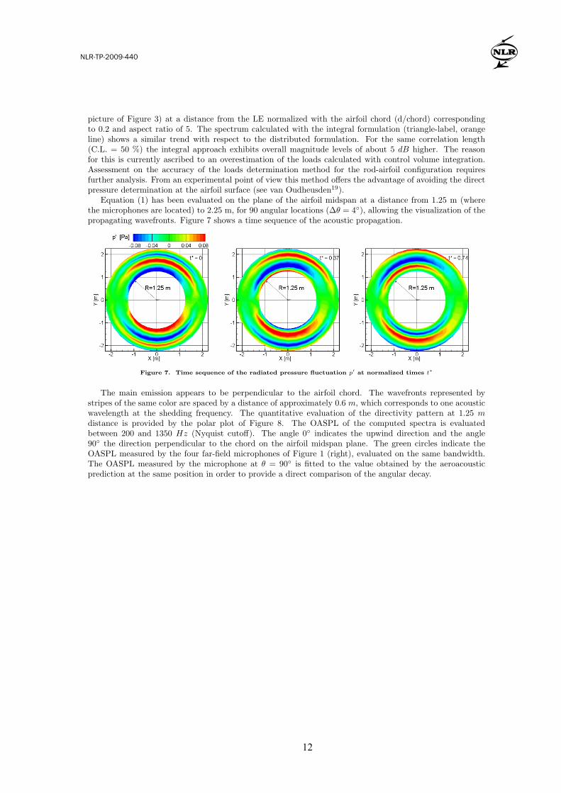
Equation (1) has been evaluated on the plane of the airfoil midspan at a distance from 1.25 m (wherethe microphones are located) to 2.25 m, for 90 angular locations (∆θ = 4◦), allowing the visualization of thepropagating wavefronts. Figure 7 shows a time sequence of the acoustic propagation.

Figure 7. Time sequence of the radiated pressure fluctuation p′ at normalized times t∗

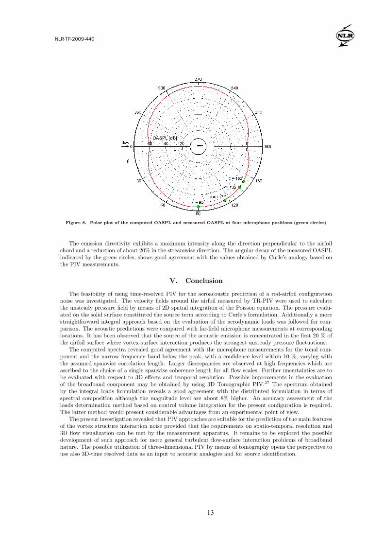
The main emission appears to be perpendicular to the airfoil chord. The wavefronts represented bystripes of the same color are spaced by a distance of approximately 0.6 m, which corresponds to one acousticwavelength at the shedding frequency. The quantitative evaluation of the directivity pattern at 1.25 mdistance is provided by the polar plot of Figure 8. The OASPL of the computed spectra is evaluatedbetween 200 and 1350 Hz (Nyquist cutoff). The angle 0◦ indicates the upwind direction and the angle90◦ the direction perpendicular to the chord on the airfoil midspan plane. The green circles indicate theOASPL measured by the four far-field microphones of Figure 1 (right), evaluated on the same bandwidth.The OASPL measured by the microphone at θ = 90◦ is fitted to the value obtained by the aeroacousticprediction at the same position in order to provide a direct comparison of the angular decay.

10 of 12


NLR-TP-2009-440

13

Figure 8. Polar plot of the computed OASPL and measured OASPL at four microphone positions (green circles)

The emission directivity exhibits a maximum intensity along the direction perpendicular to the airfoilchord and a reduction of about 20% in the streamwise direction. The angular decay of the measured OASPLindicated by the green circles, shows good agreement with the values obtained by Curle’s analogy based onthe PIV measurements.

V. Conclusion

The feasibility of using time-resolved PIV for the aeroacoustic prediction of a rod-airfoil configurationnoise was investigated. The velocity fields around the airfoil measured by TR-PIV were used to calculatethe unsteady pressure field by means of 2D spatial integration of the Poisson equation. The pressure evalu-ated on the solid surface constituted the source term according to Curle’s formulation. Additionally a morestraightforward integral approach based on the evaluation of the aerodynamic loads was followed for com-parison. The acoustic predictions were compared with far-field microphone measurements at correspondinglocations. It has been observed that the source of the acoustic emission is concentrated in the first 20 % ofthe airfoil surface where vortex-surface interaction produces the strongest unsteady pressure fluctuations.

The computed spectra revealed good agreement with the microphone measurements for the tonal com-ponent and the narrow frequency band below the peak, with a confidence level within 10 %, varying withthe assumed spanwise correlation length. Larger discrepancies are observed at high frequencies which areascribed to the choice of a single spanwise coherence length for all flow scales. Further uncertainties are tobe evaluated with respect to 3D effects and temporal resolution. Possible improvements in the evaluationof the broadband component may be obtained by using 3D Tomographic PIV.27 The spectrum obtainedby the integral loads formulation reveals a good agreement with the distributed formulation in terms ofspectral composition although the magnitude level are about 8% higher. An accuracy assessment of theloads determination method based on control volume integration for the present configuration is required.The latter method would present considerable advantages from an experimental point of view.

The present investigation revealed that PIV approaches are suitable for the prediction of the main featuresof the vortex structure interaction noise provided that the requirements on spatio-temporal resolution and3D flow visualization can be met by the measurement apparatus. It remains to be explored the possibledevelopment of such approach for more general turbulent flow-surface interaction problems of broadbandnature. The possible utilization of three-dimensional PIV by means of tomography opens the perspective touse also 3D-time resolved data as an input to acoustic analogies and for source identification.

11 of 12


NLR-TP-2009-440

14

Acknowledgments

This work is carried out within the FLOVIST project (Flow Visualization Inspired Aeroacoustics withTime Resolved Tomographic Particle Image Velocimetry) funded by the European Research Council (ERC)grant # 202887. Dr. Christophe Schram and prof. Mico Hirschberg are acknowledged for the insightfulcomments.

References

1Jacob, M. C., Boudet, J., Casalino, D., and Michard, M., “A rod-airfoil experiment as benchmark for broadband noisemodeling,” Theoretical and Computational Fluid Dynamics, Vol. 19, 2004, pp. 171–196.

2Casalino, D., Jacob, M., and Roger, M., “Prediction of rod-airfoil interaction noise using the Ffowcs-Williams-Hawkingsanalogy,” AIAA, Vol. 41, No. 2, 2003, pp. 182–191.

3Jacob, M., Ciardi, M., Gamet, L., Greschner, B., Moon, Y. J., and Vallet, I., “Assessment of CFD broadband noisepredictions on a rod-airfoil benchmark computation,” AIAA, 2008-2899 , 2008.

4Seiner, J. M., “A new rational approach to jet noise reduction,” Theoretical and Computational Fluid Dynamics, Vol. 10,1997, pp. 373–383.

5Seiner, J. M. and K., P. M., “Jet noise measurements using PIV,” 5th AIAA/CEAS Aeroacoustic Conference, Vol. AIAA-99-1869, 1999.

6Goldstein, M. E., Aeroacoustics, McGraw-Hill, New York, 1976.7Wernet, “Temporally resolved PIV for space-time correlations in both cold and hot jet flows,” Measurement Science and

Technology, Vol. 18, 2007, pp. 1387–1403.8Schroder, W., Dierksheide, U., Wolf, J., Herr, M., and Kompenhans, J., “Investigation on trailing-edge noise sources by

means of high-speed PIV,” 12th international Symposium on Application of Laser Techniques to Fluid Mechanics, 2004.9Howe, M. S., “Trailing edge noise at low Mach numbers,” Journal of Sound and Vibration, Vol. 225, 1999, pp. 211–238.

10Henning, A., Kaepernick, K., Ehrenfried, K., Koop, L., and Dillman, A., “Investigation of aeroacoustic noise generation bysimultaneous particle image velocimetry and microphone measurements,” Experiments in Fluids, Vol. 45, 2008, pp. 1073–1085.

11Schram, C., Taubitz, S., Anthoine, J., and Hirschberg, “Theoretical/empirical prediction and measurement of the soundproduced by vortex pairing in a low Mach number jet,” Journal of Sound and Vibration, Vol. 281, 2005, pp. 171–187.

12Powell, A., “Theory of vortex sound,” Journal of the Acoustical Society of America, Vol. 36, No. 1., 1964, pp. 177–195.13Mohring, W., “On vortex sound at low Mach number,” Journal of Fluid Mechanics, Vol. 85, 1978, pp. 685–691.14Haigermoser, C., “Application of an aeroacoustic analogy to PIV data from rectangular cavity flow,” Experiments in

Fluids, 2009, 00348-009-0642-5.15Lighthill, M. J., “On sound generated aerodynamically, Part I: General theory,” Proc. Roy. Soc. Lon., Vol. A 211, 1952,

pp. 564–587.16Curle, N., “The influence of solid boundaries upon aerodynamic sound,” Proc. Roy. Soc. Lon., Vol. A 231, 1955, pp. 505–

514.17Wang, M., Freund, J. B., and Lele, K. L., “Computational prediction of flow-generated sound,” Annual review of FLuid

Mechanics, Vol. 38, 2006, pp. 483–512.18Kurtulus, D. F., Scarano, F., and David, L., “Unsteady aerodynamics forces estimation on a square cylinder by TR-PIV,”

Experiments in Fluids, Vol. 42, 2007, pp. 185–196.19van Oudheusden, B. W., “PIV-based forces and pressure measurements,” Recent advances in Particle Image Velocimetry,

Vol. LS 2007-09, von Karman Institute, Rhode-St-Genese, 2009.20Liu, X. and Katz, J., “Instantaneous pressure and material acceleration measurements using a four-exposure PIV system,”

Experiments in Fluids, Vol. 41, 2006, pp. 227–240.21de Kat, R., van Oudheusden, B. W., and Scarano, F., “Instantaeous planar pressure field determination around a square-

section cylinder based on time-resolved stereo PIV,” 14th Int Symposium on the Application of Laser Techniques to FluidMechanics, Lisbon, Portugal, July 2008.

22Scarano, F. and Riethmuller, M. L., “Iterative multigrid approach in PIV image processing,” Exp.Fluids, Vol. 26, 1999,pp. 513–523.

23Roger, M. and Moreau, S., “Trailing edge measurements and prediction for subsonic loaded fan blades,” AIAA 2002-2460 ,Vol. 85, 2002.

24Lorenzoni, V., Tuinstra, M., and Scarano, F., “Combined PIV and acoustic measurements on a rod-airfoil configuration.Pilot test of the FLOVIST project,” Tech. rep., Nationaal Lucht-en Ruimtevaart laboratorium (NLR), 2008.

25Lorenzoni, V., Aeroacoustic investigation of rod-airfoil noise based on time-resolved PIV , Master’s thesis, TU Delft,2008.

26Casalino, D., Analytical and numerical methods in vortex-body aeroacoustics, Ph.D. thesis, Politecnico di Torino etL’Ecole Centrale de Lyon, 2002.

27Elsinga, G. E., Scarano, F., Wieneke, B., and van Oudheusden, B. W., “Tomographic particle image velocimetry,” Exp.Fluids, Vol. 41, 2006, pp. 933–947.

12 of 12


aeroacoustic analysis of a rod-airfoil flow by means of … · 2017-01-30 · test conﬂguration...

Documents