automatic conflguration of real-time operating systems and
TRANSCRIPT

PUniversity of Paderborn, GermanyProf. Dr. rer. nat. Franz J. RammigComputer Science, Design of Parallel Systems
Carsten Boke
Automatic Configuration ofReal-Time Operating Systems andReal-Time Communication Systemsfor Distributed Embedded Applications
Address of the author:Carsten BokeHeinz Nixdorf InstituteUniversity of PaderbornDesign of Parallel Systems GroupFurstenallee 11D-33102 Paderborn, Germany
email: [email protected]
Bibliographic notes:Carsten Boke:Automatic Configuration of Real-Time Operating Systems and Real-Time Communica-tion Systems for Distributed Embedded ApplicationsHeinz Nixdorf Institute, Paderborn, GermanyHNI-Verlagsschriftenreihe No. 142/2004ISBN 3-935433-51-4http://wwwhni.uni-paderborn.de/
Also:Submitted as a dissertation to the Faculty of Computer Science, Electrical Engineering,and Mathematics of the University of Paderborn, Germany.Supervisors:
1. Prof. Dr. rer. nat. Franz J. Rammig, University of Paderborn2. Prof. Dr. rer. nat. Odej Kao, University of Paderborn
Date of public examination: 19th December, 2003
Keywords:Operating systems, embedded systems, distributed systems, communication, real-time,configuration, customisation, analysis, schedulability, software design, software synthe-sis.
c© Carsten Boke, Paderborn 2003

Automatic Configuration of Real-Time Operating Systemsand Real-Time Communication Systems for Distributed
Embedded Applications
Dissertation
A thesis submitted to theFaculty of Computer Science, Electrical Engineering, and Mathematics
of theUniversity of Paderborn
in partial fulfilment of the requirements for thedegree of Dr. rer. nat.
Carsten Boke
Paderborn, GermanyOctober 30, 2003

Supervisors:
1. Prof. Dr. rer. nat. Franz J. Rammig, University of Paderborn
2. Prof. Dr. rer. nat. Odej Kao, University of Paderborn
Date of public examination: December 19, 2003

Acknowledgements
This work was carried out during my time at the HEINZ NIXDORF INSTITUTE (HNI),an interdisciplinary centre of research and technology of the University of Paderborn,Germany. I like to thank all my colleagues who helped me to make this work a success. Iam greatful to them all, not just for their technical support, but more importantly, for theexperiences I shared with them.
First of all, I would like to express my gratitude to Prof. Dr. Franz J. Rammig and Prof. Dr.Odej Kao for supervising and vice-supervising this work, respectively. I sincerly thankProf. Rammig for the helpful advices and direction he has given me, for his support andconstant guidance during this work. Within his working group I had the opportunity toestablish and to work on different research projects and to advice students. I was luckyenough to work in a heterogeneous working group, where I did not just benefit fromthe different research areas of my colleagues, but where I personally enjoyed that manycolleagues came from foreign countries.
I like to thank my colleagues who helped me in different ways to realise this project andgave me a good time at the institute. Due to their wide range of interest, knowledge, andresearch projects they all brought in different aspects to my work.
I like to thank Dr. Carsten Ditze, who founded the basis for my thesis. It was a pleasurefor me to contribute to and to learn from a lot of discussions with him about his design ofthe underlying operating system DREAMS. Thanks also to Dr. Thomas Lehmann for hisco-operation during the project. In the same way I owe a significant debit of gratitude toDr. Ramakrishna Prasad Chivukula, who supported me during the end of my work. Itwas alo a pleasure for me to share my office with Simon Oberthur and to talk with himabout future extensions to TEReCS. I enjoyed greatfully all the discussions and the timewith them.
Furthermore, I have to thank all readers of my thesis who helped me not only to fixtechnical parts. Special thanks here again to Dr. Prasad Chivukula and to Prof. PramodChandra P. Bhatt, who revised major parts of the document.
But writing this thesis would not have been possible without the support of additionalwonderful people. At the top of the list has to be my dear wife Deina. She supported

me with a lot of patience and encouraged me always when my confidence and patienceran low. Additionally, she had most understanding when we would have preferred to doother things together.
The closing and also very important dedications go to my dear parents Barbel and Fritz.Without their never ending support and care it would be questionable if I would everhave come so far.
The work on TEReCS had also been supported under the Priority Programme 1040“Entwurf und Entwurfsmethodik eingebetteter Systeme” by the Deutsche Forschungs-gemeinschaft (DFG) under contract RA 612/4 with the title “Entwurf konfigurierbarer,echtzeitfahiger Kommunikationssysteme”.
Paderborn, October 2003.

Contents
List of Figures . . . . . . . . . . . . . . . . . . . . . . . . . . . . . . . . . . . . . . . IX
List of Tables . . . . . . . . . . . . . . . . . . . . . . . . . . . . . . . . . . . . . . . XIII
Abstract . . . . . . . . . . . . . . . . . . . . . . . . . . . . . . . . . . . . . . . . . . 1
1. Summary . . . . . . . . . . . . . . . . . . . . . . . . . . . . . . . . . . . . . . . . 3
2. Introduction . . . . . . . . . . . . . . . . . . . . . . . . . . . . . . . . . . . . . . 7
2.1 Motivation . . . . . . . . . . . . . . . . . . . . . . . . . . . . . . . . . . . . . 7
2.2 Problem . . . . . . . . . . . . . . . . . . . . . . . . . . . . . . . . . . . . . . 12
2.2.1 Assumptions and Ignored Issues . . . . . . . . . . . . . . . . . . . . 12
2.3 Extensible µ-Kernels versus Configurable Library Operating Systems . . . 14
2.4 Operating System versus Communication System Configuration . . . . . 14
2.5 Chapter Outline . . . . . . . . . . . . . . . . . . . . . . . . . . . . . . . . . . 15
2.6 Hints for Reading . . . . . . . . . . . . . . . . . . . . . . . . . . . . . . . . . 16
3. Configuration . . . . . . . . . . . . . . . . . . . . . . . . . . . . . . . . . . . . . 19
3.1 Aims of Configuration . . . . . . . . . . . . . . . . . . . . . . . . . . . . . . 19
3.1.1 Technical Systems . . . . . . . . . . . . . . . . . . . . . . . . . . . . 22
3.1.2 Software Management . . . . . . . . . . . . . . . . . . . . . . . . . . 23
3.1.3 Software Synthesis . . . . . . . . . . . . . . . . . . . . . . . . . . . . 24
3.2 Configuration vs. Customisation and Adaptation . . . . . . . . . . . . . . 26
3.3 Methodologies . . . . . . . . . . . . . . . . . . . . . . . . . . . . . . . . . . . 27

VI Contents
3.3.1 Searching in Graphs . . . . . . . . . . . . . . . . . . . . . . . . . . . 29
3.3.2 Special Search Strategies by Defining Cost Functions . . . . . . . . 35
3.3.3 Overview of Configuration Approaches . . . . . . . . . . . . . . . . 36
3.4 Literature Survey . . . . . . . . . . . . . . . . . . . . . . . . . . . . . . . . . 41
3.5 Advantages of Configuration within a Real-Time Operating System . . . . 46
3.5.1 Goals of Operating System Configuration . . . . . . . . . . . . . . . 46
3.5.2 Examples . . . . . . . . . . . . . . . . . . . . . . . . . . . . . . . . . 48
3.5.3 State of the Art . . . . . . . . . . . . . . . . . . . . . . . . . . . . . . 48
3.6 Advantages of Configuration within a Real-Time Communication System 52
3.6.1 Goals of Communication System Configuration . . . . . . . . . . . 53
3.6.2 Examples . . . . . . . . . . . . . . . . . . . . . . . . . . . . . . . . . 53
3.6.3 State of the Art . . . . . . . . . . . . . . . . . . . . . . . . . . . . . . 54
3.7 Contribution of the Chapter . . . . . . . . . . . . . . . . . . . . . . . . . . . 59
4. Real-Time Analysis . . . . . . . . . . . . . . . . . . . . . . . . . . . . . . . . . . 61
4.1 Real-Time versus Non-Real-Time . . . . . . . . . . . . . . . . . . . . . . . . 61
4.1.1 Definition of Real-Time System . . . . . . . . . . . . . . . . . . . . . 64
4.2 Real-Time Analysis for Process Scheduling . . . . . . . . . . . . . . . . . . 65
4.2.1 Definitions . . . . . . . . . . . . . . . . . . . . . . . . . . . . . . . . . 66
4.2.2 Approaches . . . . . . . . . . . . . . . . . . . . . . . . . . . . . . . . 68
4.3 Servers for Aperiodic Tasks . . . . . . . . . . . . . . . . . . . . . . . . . . . 74
4.4 Real-Time Analysis for Communication . . . . . . . . . . . . . . . . . . . . 76
4.4.1 Definitions . . . . . . . . . . . . . . . . . . . . . . . . . . . . . . . . . 77
4.4.2 Approaches . . . . . . . . . . . . . . . . . . . . . . . . . . . . . . . . 78
4.5 Resource Constraints . . . . . . . . . . . . . . . . . . . . . . . . . . . . . . . 85
4.6 Contribution of the Chapter . . . . . . . . . . . . . . . . . . . . . . . . . . . 88
5. From Taxonomy Towards Configuration Space . . . . . . . . . . . . . . . . . 89
5.1 Taxonomy for Real-Time Systems . . . . . . . . . . . . . . . . . . . . . . . . 90
5.1.1 System Model and System Behaviour . . . . . . . . . . . . . . . . . 91
5.1.2 Task Characteristics . . . . . . . . . . . . . . . . . . . . . . . . . . . 92
5.1.3 Communication Characteristics . . . . . . . . . . . . . . . . . . . . . 93
5.1.4 Machine and Hardware Properties . . . . . . . . . . . . . . . . . . . 94
5.2 Configuration Items . . . . . . . . . . . . . . . . . . . . . . . . . . . . . . . . 95
5.3 Creating the Configuration Space . . . . . . . . . . . . . . . . . . . . . . . . 97
Contents VII
5.4 “Puppet Configuration” . . . . . . . . . . . . . . . . . . . . . . . . . . . . . 100
5.5 Conclusion . . . . . . . . . . . . . . . . . . . . . . . . . . . . . . . . . . . . . 102
5.6 Contribution of the Chapter . . . . . . . . . . . . . . . . . . . . . . . . . . . 104
6. TEReCS . . . . . . . . . . . . . . . . . . . . . . . . . . . . . . . . . . . . . . . . 105
6.1 Overview . . . . . . . . . . . . . . . . . . . . . . . . . . . . . . . . . . . . . . 106
6.2 Concept . . . . . . . . . . . . . . . . . . . . . . . . . . . . . . . . . . . . . . . 107
6.3 Model . . . . . . . . . . . . . . . . . . . . . . . . . . . . . . . . . . . . . . . . 108
6.3.1 Hardware . . . . . . . . . . . . . . . . . . . . . . . . . . . . . . . . . 108
6.3.2 Software . . . . . . . . . . . . . . . . . . . . . . . . . . . . . . . . . . 108
6.3.3 Inter-Component Model Structure . . . . . . . . . . . . . . . . . . . 109
6.3.4 Constraints . . . . . . . . . . . . . . . . . . . . . . . . . . . . . . . . 110
6.3.5 Specification of System Requirements . . . . . . . . . . . . . . . . . 111
6.3.6 Example . . . . . . . . . . . . . . . . . . . . . . . . . . . . . . . . . . 112
6.4 Design Process . . . . . . . . . . . . . . . . . . . . . . . . . . . . . . . . . . . 112
6.4.1 Methodology . . . . . . . . . . . . . . . . . . . . . . . . . . . . . . . 113
6.4.2 Synthesis . . . . . . . . . . . . . . . . . . . . . . . . . . . . . . . . . . 114
6.4.3 Configuration Algorithm . . . . . . . . . . . . . . . . . . . . . . . . 115
6.5 Hierarchical and Dynamic Configuration . . . . . . . . . . . . . . . . . . . 119
6.5.1 Hierarchical Clustering . . . . . . . . . . . . . . . . . . . . . . . . . 120
6.5.2 Dynamic Aspect . . . . . . . . . . . . . . . . . . . . . . . . . . . . . 122
6.5.3 Results of Clustering . . . . . . . . . . . . . . . . . . . . . . . . . . . 124
6.6 Description Languages . . . . . . . . . . . . . . . . . . . . . . . . . . . . . . 124
6.6.1 Describing the Design Space of DREAMS with the TEReCS Model . 126
6.7 Knowledge Transfer from the Application to the Configurator . . . . . . . 132
6.8 Real-Time Analysis . . . . . . . . . . . . . . . . . . . . . . . . . . . . . . . . 133
6.8.1 Scheduling Model . . . . . . . . . . . . . . . . . . . . . . . . . . . . 135
6.8.2 Time-triggered Event Scheduling Engine . . . . . . . . . . . . . . . 137
6.8.3 Example for a Time-triggered Event Schedule . . . . . . . . . . . . 138
6.8.4 Schedulability Analysis . . . . . . . . . . . . . . . . . . . . . . . . . 139
6.9 Impact of the Configuration on the Timing Analysis . . . . . . . . . . . . . 142
6.10 Impact of the Timing Analysis on the Configuration . . . . . . . . . . . . . 147
6.11 Contribution of the Chapter . . . . . . . . . . . . . . . . . . . . . . . . . . . 149
7. Results . . . . . . . . . . . . . . . . . . . . . . . . . . . . . . . . . . . . . . . . . 153
VIII Contents
7.1 Demonstrator . . . . . . . . . . . . . . . . . . . . . . . . . . . . . . . . . . . 154
8. Conclusion . . . . . . . . . . . . . . . . . . . . . . . . . . . . . . . . . . . . . . . 159
8.1 Overview of Publications of the Author Related to this Work . . . . . . . . 162
8.2 Outlook . . . . . . . . . . . . . . . . . . . . . . . . . . . . . . . . . . . . . . . 162
A. Simple Configuration Example . . . . . . . . . . . . . . . . . . . . . . . . . . . 165
B. Example for the Timing Analysis . . . . . . . . . . . . . . . . . . . . . . . . . . 177
C. Language Descriptions . . . . . . . . . . . . . . . . . . . . . . . . . . . . . . . 183
C.1 General Domain Knowledge . . . . . . . . . . . . . . . . . . . . . . . . . . . 183
C.2 Hardware and Topology . . . . . . . . . . . . . . . . . . . . . . . . . . . . . 188
C.3 Requirements Specification . . . . . . . . . . . . . . . . . . . . . . . . . . . 190
Index Register . . . . . . . . . . . . . . . . . . . . . . . . . . . . . . . . . . . . . . . 192
Bibliography . . . . . . . . . . . . . . . . . . . . . . . . . . . . . . . . . . . . . . . . 192

List of Figures
1.1 TEReCS is mainly built on two basic concepts: configuration and timinganalysis. . . . . . . . . . . . . . . . . . . . . . . . . . . . . . . . . . . . . . . 4
2.1 Embedded systems in modern automobiles. . . . . . . . . . . . . . . . . . . 7
2.2 From monolithic and static operating systems towards highly flexible andconfigurable ones. . . . . . . . . . . . . . . . . . . . . . . . . . . . . . . . . . 8
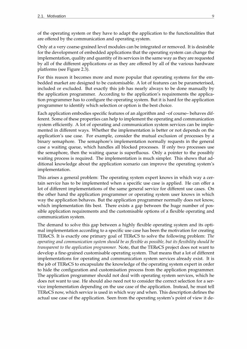
2.3 Existence of design freedom for the application, operating system andhardware platform. . . . . . . . . . . . . . . . . . . . . . . . . . . . . . . . . 10
2.4 The reduction of design freedom for the operating system by integratingrequirements from the application and the underlying hardware. . . . . . 11
2.5 The operating system configuration constraints the design space and com-pletes the operating system description to a final instantiation. . . . . . . . 11
3.1 Input/output flow for the configuration of technical systems. . . . . . . . 21
3.2 Example for a transformation of a general AND/OR-tree to its canonicalform. . . . . . . . . . . . . . . . . . . . . . . . . . . . . . . . . . . . . . . . . 30
3.3 Example for a problem reduction graph. . . . . . . . . . . . . . . . . . . . . 31
3.4 Examples for the traversal paths, if depth first search (DFS) or breadth firstsearch (BFS) is applied to a sample graph until first solution is found. . . . 32
3.5 General Best-First Search (GBF) algorithm. . . . . . . . . . . . . . . . . . . 33
3.6 GBF∗ algorithm, if heuristic h(n) is optimistic. . . . . . . . . . . . . . . . . 34
3.7 Hierarchy of BF algorithms for searching in AND/OR-trees. . . . . . . . . 36
3.8 Algorithm of the configuration cycle in PLAKON. . . . . . . . . . . . . . . . 43
4.1 Processor demand when deadlines are less than periods. . . . . . . . . . . 74
4.2 The DQDB network topology. . . . . . . . . . . . . . . . . . . . . . . . . . . 80
X List of Figures
4.3 The FDDI token ring topology. . . . . . . . . . . . . . . . . . . . . . . . . . 81
4.4 An example for a multi-hop network. . . . . . . . . . . . . . . . . . . . . . 81
4.5 The topology of a communication bus, like CAN. A message that is sentby one station can be received simultaneously by all stations. . . . . . . . . 83
5.1 OR-DAG that is representing one possible real-time communication stack. 98
5.2 Technique in an OR-DAG for eventually omitting a service B. . . . . . . . 99
5.3 The basic idea of “Puppet Configuration”. . . . . . . . . . . . . . . . . . . . . 101
6.1 Example for an Universal Resource Service Graph. . . . . . . . . . . . . . . 109
6.2 Example for the integration of Universal Service Graph, Universal Re-source Graph and Resource Graph. . . . . . . . . . . . . . . . . . . . . . . . 112
6.3 Methodology in TEReCS for creating a configuration and assembling thecode for a run-time system. . . . . . . . . . . . . . . . . . . . . . . . . . . . 113
6.4 Synthesis process in TEReCS. . . . . . . . . . . . . . . . . . . . . . . . . . . 114
6.5 “Puppet Configuration” finds a solution by traversing all paths from selectedprimitives down to all terminal nodes, whereby all OR alternatives areresolved. . . . . . . . . . . . . . . . . . . . . . . . . . . . . . . . . . . . . . . 116
6.6 Example for the calculation of the costs (C) and the depth (D) of each ser-vice assuming each service has the initial (self) costs of 1 and each SAPcosts 0. The bold lines refer to the longest path. The dashed lines refer tothe same OR-group. . . . . . . . . . . . . . . . . . . . . . . . . . . . . . . . . 118
6.7 Using hierarchy for hiding cluster graphs for super-services. The super-services are abstractions of cluster graphs. . . . . . . . . . . . . . . . . . . . 121
6.8 Algorithm of the hierarchical (recursive) configuration process. . . . . . . 122
6.9 Design flow for hierarchical clustering and configuring . . . . . . . . . . . 123
6.10 Top-level clusters of DREAMS. . . . . . . . . . . . . . . . . . . . . . . . . . . 124
6.11 Description of a declaration for a service in the specification file for the USG. 125
6.12 Illustration of the major transfer rules for the modelling of DREAMS’ object-oriented customisation features within the TEReCS’ model. . . . . . . . . . 130
6.13 TEReCS model for the class hierarchy of DREAMS’ task hierarchy. . . . . . 131
6.14 TEReCS model for the integration of timers into DREAMS. . . . . . . . . . 131
6.15 Illustration of timings and execution points of the signal handling for anexecution block . . . . . . . . . . . . . . . . . . . . . . . . . . . . . . . . . . 136
6.16 Example for a time-triggered scheduling. . . . . . . . . . . . . . . . . . . . 138
6.17 Hardware architecture and task mapping, where four tasks on four pro-cessor nodes communicate via one single CAN bus. . . . . . . . . . . . . . 142
6.18 Example 1 for the time-triggered scheduling where four tasks communi-cate via one single CAN bus. . . . . . . . . . . . . . . . . . . . . . . . . . . 145

List of Figures XI
6.19 Example 2 for the time-triggered scheduling where four tasks communi-cate via one single CAN bus, but the event of the second communicationstarts much earlier. . . . . . . . . . . . . . . . . . . . . . . . . . . . . . . . . 146
6.20 Hardware architecture and task mapping, where four tasks on four pro-cessor nodes communicate via one CAN bus and one serial RS-232 peer-to-peer connection. . . . . . . . . . . . . . . . . . . . . . . . . . . . . . . . . 147
6.21 Example 3 for the time-triggered scheduling where four tasks communi-cate via one CAN bus and one serial RS-232 connection. . . . . . . . . . . . 148
7.1 Measured schedule for the transfer of 64 Bytes user data over four proces-sor nodes. The Transputer link must be requested and the Generic protocolis used. . . . . . . . . . . . . . . . . . . . . . . . . . . . . . . . . . . . . . . . 155
7.2 Measured schedule for the transfer of 64 Bytes user data over four proces-sor nodes. The Transputer link is not requested and the Generic protocol isused. . . . . . . . . . . . . . . . . . . . . . . . . . . . . . . . . . . . . . . . . 156
7.3 Measured schedule for the transfer of 64 Bytes user data over four pro-cessor nodes. The Transputer link is not requested and the Maximum Sizeprotocol is used. . . . . . . . . . . . . . . . . . . . . . . . . . . . . . . . . . . 156
7.4 Measured schedule for the transfer of 64 Bytes user data over four proces-sor nodes. The Transputer link is not requested and the Constant protocolis used. . . . . . . . . . . . . . . . . . . . . . . . . . . . . . . . . . . . . . . . 157
8.1 The design cycle of specification, configuration and analysis in TEReCS. . 160
8.2 TEReCS is conceptually embedded into an Internet-based framework forsupporting third-party developments. . . . . . . . . . . . . . . . . . . . . . 161
A.1 Example for a Resource Graph (RG). . . . . . . . . . . . . . . . . . . . . . . . 166
A.2 Example for an Universal Service Graph (USG). . . . . . . . . . . . . . . . . . 168
A.3 Example for the final configuration according to the requirement specifi-cation on page 173. . . . . . . . . . . . . . . . . . . . . . . . . . . . . . . . . 175
B.1 Visualisation of the schedules from the output of the timing analysis onpage 180f. . . . . . . . . . . . . . . . . . . . . . . . . . . . . . . . . . . . . . 181

XII List of Figures

List of Tables
3.1 Comparison of some research driven configuration tools. . . . . . . . . . . 45
3.2 Comparison of some commercial configuration tools. . . . . . . . . . . . . 46
4.1 Scheduling algorithms for aperiodic tasks. . . . . . . . . . . . . . . . . . . . 71
4.2 Summary of guarantee tests for periodic tasks. . . . . . . . . . . . . . . . . 74
4.3 Possible categorisation of media access protocols and examples for theirimplementation. . . . . . . . . . . . . . . . . . . . . . . . . . . . . . . . . . . 84
5.1 Dimensions of a taxonomy for real-time systems. . . . . . . . . . . . . . . . 90
5.2 Configuration items. . . . . . . . . . . . . . . . . . . . . . . . . . . . . . . . 96
5.3 From taxonomy to configuration items. . . . . . . . . . . . . . . . . . . . . 103

XIV List of Tables

Abstract
The design of distributed software for embedded systems in products like automobiles,trains, airplanes, ships, automatic manufacturing lines, robots, telecommunication sys-tems, etc. becomes incredibly complex due to the huge amount of parallel working andinterconnected microprocessors. Exactly their mutual in/out-dependencies and, there-fore, their implemented communications make them very complex. It is hard to analyseand predict their behaviour. But for hard real-time control the guarantee of a special be-haviour is indispensable. Especially, the operating systems, which are often required toprovide the communication functions, introduce a lot of overhead and non-determinisminto the systems.
In this thesis we develop a methodology to generate the operating systems and the com-munication system for a distributed embedded real-time application. The operating sys-tems for each node of the network and the communication system is thereby generatedfrom a customisable library operating system construction kit. The operating systems foreach microprocessor and the communication system are assembled from tuneable com-ponents of a library. This is done by a new configuration approach named Puppet Con-figuration. The final systems are highly adapted to the requirements of the application.Thus, not required functions are excluded and the remaining functions are optimallyconfigured to serve the given use case.
Additionally, the behaviour of the finally configured distributed system is analysed in or-der to ensure a temporal correct behaviour. A new Time-triggered Event Scheduling schemeis used to attain this information before the system is targeted and implemented. Bottle-necks, overload conditions, bursts, and also idle phases are detected.
The configuration phase and the analysis phase are embedded into a contemporary de-sign methodology. The configuration has impacts on the analysis and the analysis influ-ences the configuration. Both phases are executed alternately until a valid and workingconfiguration is found (or another configuration cannot be generated).
This innovative design approach of using configuration and prediction of its behaviourreveals a lot of potential for shortening the design time and, therefore, the time-to-marketof a new embedded real-time system for a distributed controlled product.


CHAPTER 1
Summary
Nowadays, distributed control replaces more and more centralised control. In modernproducts with embedded systems a number of control units are integrated. The commu-nication aspect between these control units becomes more and more complex and im-portant. In the past decades the industry and sometimes also the research have ignoredthese distributed systems due to their complexity. A lot of efforts had been spent for theanalysis and the design of local systems. However, the research community transferredits schedulability theory in some aspects to distributed systems. Nevertheless, in practicea lot of hand work is still done in order to programme distributed systems. Some of thehigh-level development tools for real-time control systems, like ASCET-SD [45], StateM-ate [64], or CAMeL [70, 107, 151], produce target code, but this must often be adapted oreven distributed to the final target by hand. This happens, because the tool does not sup-port any operating system or the one which is supported cannot be applied to the finaltarget. For this reason, the operating system services have to be programmed by hand orthe code have to be ported to another operating system or target.
In order to specify inherently parallel working applications, synchronous languages hadbeen defined. Synchronous languages are based on the simultaneity principle: In reactivesystems multiple actions or computations happen simultaneously. Languages like Lustre[58] or Esterel [12] handle the communication between parallel and distributed systemssynchronously. All processes compute one discrete time step and then they communicateat the same time. They simply define a synchronous interleaving between calculationand communication. Thereby, they assume that the communication overhead is constantand can be ignored. However, this is a very pragmatic approach and leads to severalproblems for their implementation on really distributed systems.
This thesis is related to embedded systems. The development of, especially, distributed sys-tems is supported. Real-time aspects are additionally considered. Thus, the real-time com-munication between distributed tasks on several embedded control units is mainly con-sidered. Especially, the adaptation of the target operating systems for each control unitwith its communication facilities to one specific distributed application is the main topic.

4 Chapter 1. Summary
This goal is achieved by using techniques from the configuration theory. The implementa-tion of operating and communication services can vary. A specific implementation of aservice can only work, when the environment assures certain properties. Operating sys-tem code that is written for one specific use case will be reused, whenever that use caseis detected.
Time-Triggered Event
Scheduling
Medium1 trans+ prop
Methodology
Puppet-Configuration
Fine-granular and customisable real-time OS
Configuration
TEReCS
Analysis
Primitives
URSG
Fig. 1.1: TEReCS is mainly built on two basic concepts: configuration and timing analy-sis.
This goal is achieved by applying new ideas and concepts to the design domain for dis-tributed embedded applications. A new and contemporary approach to the design ofoperating and communication systems has been developed. It is highly flexible and ex-tensible. Additionally, the memory footprint and the real-time constraints are consideredduring the design phase. The design process runs automatically, when the informationabout the application’s behaviour and its requirements are specified. The design processexploits application specific knowledge for the configuration of the operating and com-munication systems. It reduces dramatically the design time for distributed and efficientoperating and communication systems. This is due to a hierarchical and highly flexibleconfiguration concept. Additionally, the timeliness execution of all communicating tasksis checked. On the one hand, this approach supports the application designer with inter-nal knowledge about the operating systems activities in order to identify bottlenecks ofthe system design. On the other hand, the application designer must not be an operatingsystem expert in order to select or parameterise certain operating system services.
Thus, it becomes possible to support nearly all application scenarios and a huge varietyof hardware platforms with only one operating system library. The final target operatingsystems are slim and efficient, because they support exactly the application scenario andnot more. Configuration is a promising approach for software reuse.

5
Another very exceptional concept is the integration of the configuration and the timinganalysis. During the automatic design process configuration and timing analysis havemutual influences on each other. The configuration determines the operating system’soverhead, which is considered by the timing analysis, and the timing analysis may forbidcertain configuration options due to overload conditions.
All of these aspects led to the development of Tools for Embedded Real-time CommunicationSystems (TEReCS) that are described in this thesis. The tool suite consists of the followingtools:
• TGEN is the configurator
• TCLUSTER implements the hierarchical cluster-aided configuration.
• TANA is the timing analyser
• TDESIGN encapsulates the design methodology with its design cycle and callsTCLUSTER, TGEN, and TANA.
• TEDIT is an graphical editor for the domain knowledge databases that are used forthe configuration.

6 Chapter 1. Summary

CHAPTER 2
Introduction
2.1 Motivation
One of the big challenges for the development of embedded applications these days is theintegration of many co-operating applications into one or even a set of products. Nowa-days, many applications are distributed over several embedded control units (ECUs). Ex-amples are the entry of intelligent and fully automatic machines and robots into modernproduction processes and also the “computerisation” of classical transportation vehicles,like trains, airplanes and, especially, automobiles.
ABS Video
Engine Multimedia
DashBoard
DoorModule
AirCondition
ESP Navigation
Suspension Radio
Gearbox
ABS Video
Engine Multimedia
DashBoard
DoorModule
AirCondition
ESP Navigation
Suspension Radio
Gearbox
Gateway
Fig. 2.1: Embedded systems in modern automobiles.
A modern car contains up to 100 microprocessors that control systems like the powertrainwith its motor management, chassis, Anti-lock Braking System (ABS), Electronic Stabilisa-tion Programme (ESP), suspension, airbag, and gear box control, the body module with itsdashboard, indicating, lighting, seat, door, and key controllers, and the comfort module

8 Chapter 2. Introduction
with its air condition, telematics, navigation, radio, video, multimedia, telephone andInternet connectivity. The ECUs are interconnected via different communication links.Their integration is complex and sometimes absolutely critical.
All of these systems require different hardware and also different operating and com-munication services. Due to the general development process in companies, differentversions of these systems in different generations or families of a product and sometimesalso in complete different systems are implemented on top of the same microprocessorand operating system. This is mainly done in order to reuse the development know-how of the engineers and to reuse previous software developments. New hardware(microprocessors and communication links) can often only be used for a new productversion, when a development environment with an appropriate operating system sup-port is available. Often the operating systems that are used embody the virtual machineidea. Therefore, they implement a lot of general services and are more or less monolithickernel architectures with coarse-grained module extensions.
HW Abstraction Layer (HAL)
HW Abstraction Layer (HAL)
Hardware
ApplicationApplicationApplicationApplicationApplicationApplicationApplicationApplicationApplicationApplication
Run-Time Platform or
Operating System
HW Abstraction Layer (HAL)
Application
Run-Time
Platform
Communication
System
Hardware
Standard:
Many applications are
developed for a static
operating system
Goal:
Optimal adapted
run-time platform
for each application
Fig. 2.2: From monolithic and static operating systems towards highly flexible and con-figurable ones.
There is a gap between the flexibility of the application’s specification and the –more orless– monolithic operating and communication system’s implementation with its kernel,modules, and drivers. This gap is often closed by implementing the operating and com-munication system as general as possible. This means that the operating system servicesare implemented for the general use case. This results into the well known general pur-pose operating systems, like Linux or WindowsTM. Their services are implemented insuch a way, so that they can be used for a brought variety of (desktop) applications. Thisapproach implies that a lot of operating system code is unused or behaves often very inef-ficiently. A lot of overhead is incorporated into the operating and communication systemin order to handle every use case. Also, a lot of commercial real-time operating systemsare implemented in such a way, so that they can run the most real-time applications (seeSection 3.5.348). But instead of having application specific services, the application pro-grammers must cope with the predefined ones. Often they suffer from missing features
2.1. Motivation 9
of the operating system or they have to adapt the application to the functionalities thatare offered by the communication and operating system.
Only at a very coarse-grained level modules can be integrated or removed. It is desirablefor the development of embedded applications that the operating system can change theimplementation, quality and quantity of its services in the same way as they are requestedby all of the different applications or as they are offered by all of the various hardwareplatforms (see Figure 2.3).
For this reason it becomes more and more popular that operating systems for the em-bedded market are designed to be customisable. A lot of features can be parameterised,included or excluded. But exactly this job has nearly always to be done manually bythe application programmer. According to the application’s requirements the applica-tion programmer has to configure the operating system. But it is hard for the applicationprogrammer to identify which selection or option is the best choice.
Each application embodies specific features of an algorithm and –of course– behaves dif-ferent. Some of these properties can help to implement the operating and communicationsystem efficiently. A lot of operating and communication system services can be imple-mented in different ways. Whether the implementation is better or not depends on theapplication’s use case. For example, consider the mutual exclusion of processes by abinary semaphore. The semaphore’s implementation normally requests in the generalcase a waiting queue, which handles all blocked processes. If only two processes usethe semaphore, then the waiting queue is superfluous. Only a pointer to the possiblywaiting process is required. The implementation is much simpler. This shows that ad-ditional knowledge about the application scenario can improve the operating system’simplementation.
This arises a general problem: The operating system expert knows in which way a cer-tain service has to be implemented when a specific use case is applied. He can offer alot of different implementations of the same general service for different use cases. Onthe other hand the application programmer or operating system user knows in whichway the application behaves. But the application programmer normally does not know,which implementation fits best. There exists a gap between the huge number of pos-sible application requirements and the customisable options of a flexible operating andcommunication system.
The demand to solve this gap between a highly flexible operating system and its opti-mal implementation according to a specific use case has been the motivation for creatingTEReCS. It is exactly one primary goal of TEReCS to solve the following problem: Theoperating and communication system should be as flexible as possible, but its flexibility should betransparent to the application programmer. Note, that the TEReCS project does not want todevelop a fine-grained customisable operating system. That means that a lot of differentimplementations for operating and communication system services already exist. It isthe job of TEReCS to encapsulate the knowledge of the operating system expert in orderto hide the configuration and customisation process from the application programmer.The application programmer should not deal with operating system services, which hedoes not want to use. He should also need not to consider the correct selection for a ser-vice implementation depending on the use case of the application. Instead, he must tellTEReCS now, which service is used in which way and when. This description defines theactual use case of the application. Seen from the operating system’s point of view it de-
10 Chapter 2. Introduction
OS
Design
Space
Application
Design
Space
Hardware
Components
Application
Run-Time
Platform
Communication
System
Hardware
Fig. 2.3: Existence of design freedom for the application, operating system and hardwareplatform.
fines in which way the application behaves or wants to act. Depending on this behaviourTEReCS automatically selects the correct implementations of the required services, whichfit best to that behaviour and produce the overall minimum overhead.
The strong demand for a flexible operating system with different implementations forits services arises another problem: A lot of operating system services assume that otherspecific services are present or behave in a special way. For this reason, a lot of operat-ing system internal dependencies and requirements exist. In order to assemble a correctand most efficient operating system with minimal overhead, the application programmermust normally select the appropriate implementations of the services that are requiredfor the final application. Additionally, he must also be an operating system expert, so thathe can consider and solve these operating system internal dependencies. This mixture ofexternal or application specific knowledge and operating system internal knowledge isstrongly separated in TEReCS.
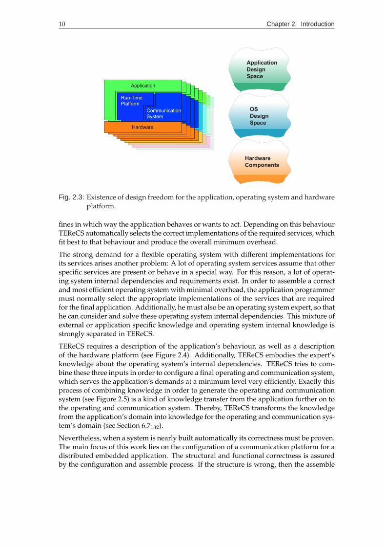
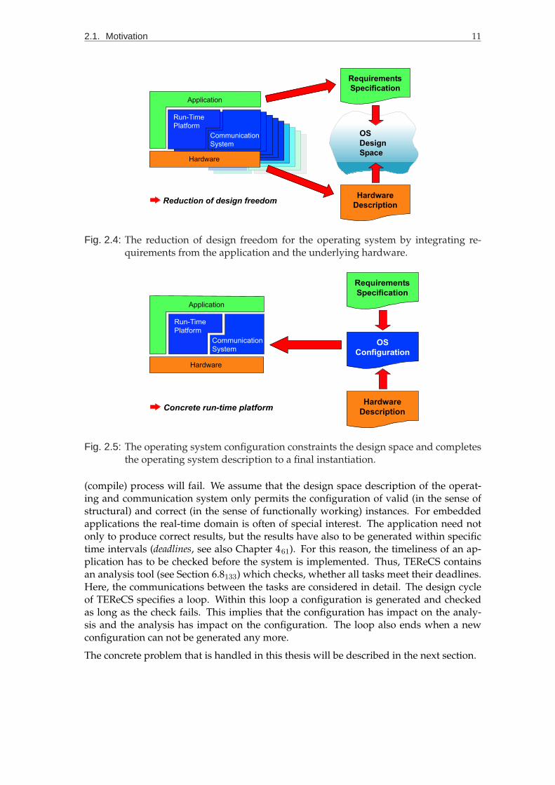
TEReCS requires a description of the application’s behaviour, as well as a descriptionof the hardware platform (see Figure 2.4). Additionally, TEReCS embodies the expert’sknowledge about the operating system’s internal dependencies. TEReCS tries to com-bine these three inputs in order to configure a final operating and communication system,which serves the application’s demands at a minimum level very efficiently. Exactly thisprocess of combining knowledge in order to generate the operating and communicationsystem (see Figure 2.5) is a kind of knowledge transfer from the application further on tothe operating and communication system. Thereby, TEReCS transforms the knowledgefrom the application’s domain into knowledge for the operating and communication sys-tem’s domain (see Section 6.7132).
Nevertheless, when a system is nearly built automatically its correctness must be proven.The main focus of this work lies on the configuration of a communication platform for adistributed embedded application. The structural and functional correctness is assuredby the configuration and assemble process. If the structure is wrong, then the assemble
2.1. Motivation 11
Run-Time
Platform
Communication
System
Application
Hardware
Requirements
Specification
Hardware
Description
OS
Design
Space
Reduction of design freedom
Fig. 2.4: The reduction of design freedom for the operating system by integrating re-quirements from the application and the underlying hardware.
Run-Time
Platform
Communication
System
Application
Hardware
OS
Configuration
Requirements
Specification
Hardware
DescriptionConcrete run-time platform
Fig. 2.5: The operating system configuration constraints the design space and completesthe operating system description to a final instantiation.
(compile) process will fail. We assume that the design space description of the operat-ing and communication system only permits the configuration of valid (in the sense ofstructural) and correct (in the sense of functionally working) instances. For embeddedapplications the real-time domain is often of special interest. The application need notonly to produce correct results, but the results have also to be generated within specifictime intervals (deadlines, see also Chapter 461). For this reason, the timeliness of an ap-plication has to be checked before the system is implemented. Thus, TEReCS containsan analysis tool (see Section 6.8133) which checks, whether all tasks meet their deadlines.Here, the communications between the tasks are considered in detail. The design cycleof TEReCS specifies a loop. Within this loop a configuration is generated and checkedas long as the check fails. This implies that the configuration has impact on the analy-sis and the analysis has impact on the configuration. The loop also ends when a newconfiguration can not be generated any more.
The concrete problem that is handled in this thesis will be described in the next section.
12 Chapter 2. Introduction
2.2 Problem
For each node of the interconnection network of a distributed target system an operatingsystem has to be generated. This thesis concentrates on the methodology for the configurationprocess of a customisable communication system and multiple customisable operating systems.These operating systems must be able to execute the tasks of each node. They must alsobe able to provide the required communication services. The communication and oper-ating systems have to be built from predefined atomic items, which must be parameterisedand connected appropriately. The totality of all available atomic items represents the com-ponent database or construction kit library for the operating systems.
The task of TEReCS is to generate for each node of the target system a configuration description.These configurations describe which atomic items of the component database have to beintegrated into the instance of the operating system of one node. Additionally, the con-figurations define all missing parameters for these items and they describe in which waythe selected items have to be connected. The main objective is to generate a solution thatis optimal in the sense of resource usage. The memory consumption and the punctualexecution must just fit in the limits that are given by the system engineer.
In order to achieve this goal the application’s requirements and behaviour, and also thehardware architecture and topology must be described by the system engineer (see Fig-ure 2.5). TEReCS contains the design space description for all valid and correct operatingsystem implementations. When the hardware platform contains redundant communica-tion connections, TEReCS automatically tries to select only the “cheapest” connectionsfor the routing of the messages that just fulfil the timing constraints.
Hand written code is still dominating for the implementation of embedded real-time ap-plications. Often, operating system functions (like device drivers and protocols) are man-ually developed from scratch. This is done in order to have optimally adapted implemen-tations that just meet the desired requirements and save as much resources (memory andprocessor time) as possible. TEReCS tries to bridge from the application’s specification to theautomatic distributed implementation on top of configurable operating systems and an integratedconfigurable communication system.
2.2.1 Assumptions and Ignored Issues
During the design process for distributed real-time applications occur obviously twomain problems, which are not covered by TEReCS. First, the load balancing of the tasksonto the processors is assumed to be done by the engineer or a third-party tool. Second,the estimation of the average or worst-case execution times of the tasks and also the esti-mation of the operating system overhead is assumed to be possible with other tools (likeCHaRy [1]). TEReCS assumes that the mapping of the tasks onto the processors and theworst-case execution times of the tasks and the operating system services are known apriori.
TEReCS wants to know from the application programmer, which tasks run on whichprocessors. It wants to known in addition their periods, their worst-case execution times,and their deadlines. It also wants to know which operating system services are called byeach task. For the timing analysis it is also desirable to know, when these system calls

2.2. Problem 13
occur relatively to the start time of the task. For the definition of these relative start timesall operating system overhead of previous calls is assumed to be zero.
Because TEReCS concentrates on the communication system, the system calls that send orreceive messages have to be marked explicitly. Additionally, the corresponding send()and receive() of two tasks have to be connected. This connection is assumed to be anuni-directional message transfer. The maximum size of the message and the period ofthe transfer (minimum message inter-arrival time) must also be given. Optionally, the datastructure of the message can be declared. If this is given, TEReCS can automatically inte-grate protocol code (when the operating system supports this) in order to transform theendianess of the data for heterogeneous hardware architectures. Also optional protocolspecifications for this communication connection can be specified. These include requestsfor error detection and correction, acknowledging, a synchronous send (rendezvous), thereceiver buffer capacity (to be there or not), a list of hardware links not to be used (thisoption is internally required between the configuration and analysis phase), and the portobject’s name that is used for the send and receive call.
TEReCS also assumes that the system behaves statically. This means that tasks do not oc-cur sporadically and are not created and terminated dynamically on demand. Such taskscan be modelled in TEReCS only when these sporadic tasks are assumed to be alwayspresent; thus resources are wasted. The tasks and the communications are assumed to beperiodic. Aperiodic or sporadic ones must have assigned a minimum period.
TEReCS was designed especially for the generation of configurations for inter-node com-municating operating systems. It is completely independent of the target operating sys-tem to be used. The only requirements a target operating system (OS) should fulfil are:
• The OS must be configurable
• The OS should support various communication protocols and devices
• The size of the objects to be configured should be of the same granularity
• The OS should be tunable at a fine-grained level (but this is not a must)
• The configuration objects are atomic
• The objects can be distinguished by type, costs, and their required sub-relationshipdependencies to other objects
• The objects must be parameterised and their dependencies to other objects are to beconfigured
• The configuration decisions can be mapped to the selection of concrete choices outof alternative objects
• The scope of the configuration should be the selection of the objects per processorand their inter-relationships
• In particular, the objective of the configuration is to build a service platformfor the application from these objects and to map the communications onto ser-vices/protocols of the operating system, real existing hardware devices, and media(resource reservation/routing) by producing minimal costs and providing a timeli-ness execution

14 Chapter 2. Introduction
2.3 Extensible µ-Kernels versus Configurable Library Operating Systems
Operating systems can be distinguished into two main categories. The first category com-prises all operating systems that integrate a kernel. The kernel embodies all basic servicesof the operating system. These are mainly the resource management functions like thedispatching of tasks to the processor, their synchronisation, and the communication. Of-ten, the code of the kernel is executed in a more privileged level of the processor in orderto maintain specific registers, which are normally protected against the application code.For this reason, the application requests for operating system functions by traps or systemcalls. These mechanisms change the privilege level and enter the kernel. The kernel alsooften maintains its own memory area, which cannot be accessed by the application tasks.This assumes that a memory management unit (MMU) exists, which can be programmedaccordingly. Kernels are distinguished into monolithic, µ-, nano-, femto-, and even pico-kernels by the amount and quality of services they offer. Additional services can often beimplemented by operating system tasks, which run outside the kernel and behave likeservers.
For configuration purposes such kernel-like operating systems support for modules anddemons that can optionally be integrated. Modules are services that are directly integratedinto the kernel during compile-time or loaded during run-time (see page 48ff.). Demonsare the operating system’s server tasks that run in the background of the applications.They can be started or terminated on demand. Another configuration option for thiscategory of operating systems is to change the complete kernel. This can mainly be doneduring the compile-time or the load-time of the kernel. The configuration options ofkernel-like operating systems are often limited and act on a very coarse-grained level.
The other category of operating systems implement their services in a code library thatis linked directly to the application code. They miss a kernel and mainly act as a serviceplatform. Often, such systems are called run-time platform instead of operating system.Their operating system services are simply requested by a function call. Examples forsuch systems are the CTools for Transputers [65] or DREAMS. DREAMS was developedespecially for the purpose to support fine-grained customisation facilities of the run-timeplatform. Therefore, DREAMS is configurable in the source code before compile-time atthe object level (for details see page 51 and Section 6.6.1.1127).
DREAMS is used for TEReCS as the target system under consideration. But DREAMS isused in TEReCS only as a demonstrator [15]. TEReCS is flexible in the way that it canbe adapted to nearly every configurable operating system, which is compliant to theproperties that are mentioned on page 13. Its input language is designed to fit for thegeneral case and also its output language can be adjusted to the required format.
Because the aspect of a distributed application and the communication dependencies arein the main focus of TEReCS, the next section will clarify what is meant by the distinctionof operating system and communication system.
2.4 Operating System versus Communication System Configuration
Generally, the communication services are an integral part of the operating system of onecomputer. In this case often only the device drivers for the communication links and the

2.5. Chapter Outline 15
implemented protocol stacks are considered. The operating system is seen from a localpoint of view. The local system is the main service and execution platform, which sup-ports for communication to externally located services on (sometimes dedicated) servers.Also the applications are local to one node. Sometimes they act as clients and requirecommunication to servers.
But in the embedded world a distributed system often implements also a distributedapplication. The interconnected network of processor nodes serves as one virtual ma-chine. Here, the global view onto the whole distributed and parallel working system ispreferred. The client/server aspect plays a minor role. The distributed tasks often havean equal status. The communication dependencies between the tasks are immanent andvery important for achieving the final goal. The interconnection network between theprocessor nodes and the operating system services on each node represent the commu-nication system. In the real-time domain not only the task scheduling on one processor,but also the global scheduling on all processors, as well as the scheduling of the mes-sages on the links have to be considered and analysed in order to assure a temporalcorrect behaviour. The view to an operating system, which has a communication systemintegrated, can completely be inverted: Here, the communication system of the virtualdistributed machine has many local operating system instances integrated on each pro-cessor node.
TEReCS uses the second global view. The main focus of TEReCS lies on the generation ofoptimally adapted local operating system instances. The communication dependenciesbetween the distributed tasks are mainly considered. Moreover, it is the main motiva-tion for TEReCS to support an optimal and temporal correct communication inside thedistributed virtual machine. The communication aspect mainly drives the configurationand analysis in TEReCS. This is the reason why in this thesis the words operating systemand communication system are often used in conjunction or are explicitly be distinguished.
2.5 Chapter Outline
The following list provides a closer view on the organisation and intentions of each chap-ter.
Chapter 1 starts with a summary.
Chapter 2 contains an introductive overview over the topic and gives the motivation forthis thesis. The problem, which TEReCS tries to solve, is explained herein.
Chapter 3 refers to “Configuration” in general. In that chapter the general theory aboutconfiguration is presented. Additionally, it gives a short overview about existingconfiguration systems, as well as an overview about configurable operating sys-tems.
Chapter 4 presents a general and brief overview about the state of the art in “Real-timeAnalysis”. This chapter presents a reasonable good introduction to the schedula-bility theory of real-time systems. It is important to have this overview in order tounderstand the problem, which TEReCS has to solve in this domain. The theory ofprocess scheduling is extended by approaches that handle communication aspects.

16 Chapter 2. Introduction
Chapter 5 tries to give an answer for the question: How is it possible to come “froma taxonomy” for operating systems “towards their configuration space”? Such acomplete design space description of the operating system under consideration isrequired by our configuration tool TEReCS. The idea of the “Puppet Configuration”process in TEReCS is developed in this chapter.
Chapter 6 is mainly dedicated to the herein developed tool suite TEReCS. A model andmethod is presented for an automatic configuration process (see Section 6.3 andSection 6.4). In this model the detailed information about the structural proper-ties of the configurable communication and operating system are hidden from theuser. The configuration process is extended by a hierarchy concept in Section 6.5.The languages for the inputs of TEReCS’ configurator and analyser are briefly de-scribed in Section 6.6. Hereafter, the knowledge transfer from the application toTEReCS in order to configure the operating systems and the communication systemis explained (see Section 6.7). In Section 6.8 the concept of the real-time analysis inTEReCS is presented. The chapter ends with some examples that show the mutualinfluence of the configuration (see Section 6.9) and analysis phase (see Section 6.10)in TEReCS.
Chapter 7 presents briefly some results that can be achieved by using TEReCS’ method-ology.
Chapter 8 concludes this thesis with an outlook.
The Appendix refers to a simple configuration example, as well as one for the timinganalysis. A description of the input languages for TEReCS is also given.
Each main chapter ends with a summary that describes the contribution of that chapterto this thesis.
2.6 Hints for Reading
The Chapter 3 and the Chapter 4 give an introductive overview about configuration andreal-time analysis. Readers who are familiar with these topics can skip the chapters. TheChapter 2, Chapter 5, Chapter 6, and Chapter 7 should be read in the given order.
The thesis also addresses topics in the fields of operating systems, embedded systems,real-time control, communication, and object-oriented design. It is assumed that thereader is familiar with the basic concepts and terms in these areas.
The index register can be consulted to expand abbreviations that are used. Some indexentries may be of special interest:
Operating system contains a list of presented operating systems.
TEReCS contains a list of all explicitly defined new terms concerning TEReCS.
Configuration enumerates several concepts for this topic
Configuration system lists the existing configuration systems that are described in this the-sis.

2.6. Hints for Reading 17
To ease locating references to figures, tables, and subsections, far away references areindexed by the corresponding page number, like Section 6.9142.
The Appendix A and the Appendix B give two simple examples for the inputs and out-puts to the configurator TGEN and the timing analyser TANA, respectively.

18 Chapter 2. Introduction
CHAPTER 3
Configuration
A configuration system is an expert system which helps to assemble components intoan aggregate according to some goal specification and using expert knowledge.
Bernhard Neumann, 1988 [91, p. 4]
This chapter wants to introduce the theory of configuration and, additionally, some prac-tical systems are presented. At the beginning the aims and the meaning of configurationare clarified. The overall goal of configuration in different application domains is de-scribed. Then, a detailed presentation of the methodologies that can be used for config-uration are presented. The different approaches are classified after their representationmodels and their algorithms. The inputs and outputs to the configuration algorithms aredescribed in general. A survey of existing configuration systems completes this chapter.Of coarse, an overview about the advantages and aspects of configuration for operat-ing systems and for communication systems follow. Herein, also some already existingoperating systems that make use of configuration are presented.
At the end of the chapter the reader will understand the problem that configurationsolves and he will have an overview about the different approaches that can be used toachieve this goal. He will also have an idea of the aspects where configuration can helpto construct operating and communication systems for special use cases. The first sectionof this chapter starts with an overview about the aims in general, why configuration isused instead of other techniques for building a final tailor-made system.
3.1 Aims of Configuration
The overall aim why a system or a component is designed to be configurable is the strong MeetRequire-ments
desire to save costs in realising the final system. The scope of costs may comprise ofspace, weight, execution time, power, energy consumption or some other resource needs.

20 Chapter 3. Configuration
Moreover, it is intended that the system’s properties meet as closely as possible the re-quirements of an application or an environment. This means a final configuration of thesystem measured in terms of a cost function should fit best and should match all struc-tural, functional, resource and timing requirements.
Additionally, a configurable system can support reuse of its components for differentReuseComponents implementations. All similar implementations serve the general purpose, where the sys-
tem exists for, but can be distinguished in their internal structure, functionality, costs andquality of service (QoS) they provide. This is based on the idea that different requirementsshould be served by different (optimally adapted) systems and, therefore, save resources(or costs) for unused features.
The requirements that a final system has to comply are specified by a requirements spec-AssembleSystem ification. In a formal way all requested final properties that the system has to fulfil are
described herein. It is the task of the configuration process to assemble the correct (andminimal) set of components with the correct arrangement that has these properties (andserves for the required functionalities) at minimal costs.
Often the requirements specification evolves dynamically during the configuration pro-Guide Usercess. Thus, the configurator interactively asks for certain properties the final systemshould have. In this case it is the task of the configurator to guide the users throughthe process. Only valid choices and actually valid property options are presented.
Additionally, the configurator takes care of the correctness, i.e. the final system worksAssureCorrectness and behaves in the appropriate and desired way. This includes that the configurator is
aware of structural inter-component relationships such as “a component A can only work,if another component B is present” (implication). Such relationships, constraints, or rulesare specified within a database. This database serves as a knowledge base, which storesall domain specific knowledge about the dependencies and properties of the system’scomponents. Within the algorithm of the configuration process the (domain’s) controlknowledge is stored, which defines how a final configuration can be derived by selectingappropriate components and fulfilling the requirements specification (see Figure 3.1).
A configuration algorithm that dynamically requires user interaction is called interactiveAutomaticConfiguration configuration process. On the other hand, a requirements specification can be provided as
static input to the configuration tool before the configuration process starts. If the config-urator requires no other user interaction in order to create the configuration of the finalsystem, it is considered to be an automatic configuration process.
In order to support for a highly flexible system, that can be adapted to certain require-Hide ExpertKnowledge ments, a component library with customisation features and the expert knowledge about
the assembly process is required. This expert knowledge comprises the static informa-tion about the component’s interrelationships and customisable properties, as well as thecontrol knowledge of the process. A configuration tool can hide this expert knowledge –which includes a lot of implementation details of a system – from a user (who wants touse a finally configured system with certain properties).
In this way configuration provides an abstraction of the system. Thus, just as operatingProvideSystem
Abstractionsystems provide a virtual machine (hiding all information of the concrete hardware) byits API, the configuration tool provides a virtual view to the system by its requirementsspecification. Nevertheless, the idea of supporting different resources can be supportedby the configuration tool. The system itself and the application can be planned inde-

3.1. Aims of Configuration 21
Assembly
ConfigurationProcess
ControlKnowledge
+
DomainKnowledgeDatabase
SystemComponentsRepository
ConfigurationDescription
User Interaction
describes
optional
ApplicationSpecific
Knowledge
RequirementSpecification
=
System
TE
Re
CS
DR
EA
MS
steers
Fig. 3.1: Input/output flow for the configuration of technical systems.
pendently from the present resources. If the system’s component library supports fordifferent types and amount of resources, then only those components will be consideredwhile configuring, which satisfies the given resource requirements. Or seen from thebottom: Only for the present resources the appropriate components are integrated into afinal configuration (if required).
This implies that there exists another specification, which describes the given or existingresources and constraints that the configuration can use or must satisfy. Obviously, thisspecification can be empty. But, often it exists and is also a part of the requirementsspecification.
Previously, it was mentioned that the requirements specification defines the properties a ExploitApplication-internalKnowl-edge
final configured system must fulfil and that it can be seen as an abstraction. But where dothese properties/abstractions come from? They are derived from the application. Internalknowledge about the application forms the basis for the requirements specification. In thisway, the configurator exploits the internal knowledge from the application for generatingan optimal (resource and cost minimal) system. The configuration algorithm –or morespecifically: the control knowledge– defines a knowledge transfer from the application tothe system under consideration (see Section 6.7132).
In a general sense, application’s configuration is used to support users to create newerand fully specified derivatives from customisable systems. Mainly three fields can beidentified, in which configuration is exploited to its fullest extent. These are “Techni-cal Systems”, “Software Management” and “Software Synthesis”. Whereas research con-centrates on the more natural aspect of configuration in the field of “Technical Systems”,commercial companies develop a huge variety of products in the area of “Software Man-agement”. In “Software Management” configuration is principally used to support soft-

22 Chapter 3. Configuration
ware developer teams to handle big software projects and all of their software fragments.“Technical Systems” in fact mainly drove the scientists to create a theory about configura-tion. Mostly, configurators for “Technical Systems” have been created for business servicesin order to support sales managers during the creation of (correct) sales offers for cus-tomers. Configuration for “Software Synthesis” is a quite new research topic. It is inspiredby configuration for “Technical Systems”. The configurator TGEN for TEReCS, which isdeveloped in this thesis, belongs to this area.
In the next three sections, these three areas are briefly investigated. We present, how theycan exploit configuration for specific purposes. Examples for configuration systems aregiven later on in Section 3.441 after the basic ideas and principles have been presented.
3.1.1 Technical Systems
The primary application domain for configuration systems are technical systems. A tech-nical system often consists of a variety of parts. Each part provides for some propertiesor facilities in order to yield the overall objective. Such properties or facilities can bethe component’s spatial design, weight, dimension, energy conversion mechanism (e.g.from electrical power to a physical force), melting point, thermal conductivity, or otherphysical properties. The spatial arrangement of the parts and their connections definenaturally a component structure or hierarchy. Moreover, energy or mass flows and forcescan be observed between their physical connections, which naturally define interrelation-ships and dependencies among the components.
Furthermore, it is the engineer’s natural view to build complex systems by arrangingcomponents. This procedure is known as constructing. If the components are pre-definedand are not to be created from scratch, then this procedure becomes identical to the con-figuration problem.
In fact, technical systems and the manner of their construction have been the reason whythe theory of configuration had been developed. The engineer’s desire to be supportedby a software tool drove the automation of the construction process. The engineers desirea tool, which takes care of constraints, with respect to the correct arrangement of compo-nents (by checking the dependencies). And consequently, the engineer will be replacedby such a tool, when the expert’s knowledge is completely integrated.
Many examples of this kind can be found. Here, the pioneer tool XCON (see page 41),which configures computer systems at DEC, AKON (see page 41), which configures tele-phone switchboards at Bosch/Telenorma, and artdeco (see page 44), which configureshydraulic circuits and had been developed at the University of Paderborn, should bementioned.

3.1. Aims of Configuration 23
3.1.2 Software Management
Configuration management is the key to managing and controllingthe highly complex software projects being developed today.
Clive Burrows, 1999 [24, p. 1]
Most Software Configuration Management (SCM) systems are version-oriented, where eachcomponent exists in several versions organised as variants (alternative versions) or revi-sions (consecutive versions). But Configuration Management (CM) tools have developedfrom simple version-control systems targeted for individual developers into systems ca-pable of managing developments by large teams operating at multiple sites around theworld. The key capabilities of SCM tools are the identification and control of softwareand software-related components as they change over time. The key features supportedby SCM tools are:
Parallel Working. Originally, SCM systems’ primary task is to prevent several users(programmers) from attempting to change the same component (piece of softwarecode) at the same time.
Change Management. Version control maintains a history of the changes to a compo-nent as it evolves over time and allows users to access a particular version – notjust the last version created. Moreover, the problem of tracking, change control,the presentation, and the analysis of management information derived from thesesources are issues of SCM.
Build and Release Support. An intelligent creation process can reduce build timesdramatically by reusing partially configured items from previous implementations.
Process Management. Many users, particularly those seeking an external quality ap-proval such as ISO 9000 or from a particular Software Engineering Institute havestandard development processes, which they expect their development teams tofollow. The process management features in SCM tools allow the developer to en-sure that components progress through chosen lifecycle phases before being re-leased.
Web Management. SCM support for Web and particularly Intranet pages and theirembedded objects.
Documentation Support. It is a big challenge to support for documentation of the de-cisions and work done on software projects resulting into different versions andbranches. Document management systems offer facilities to handle large and com-plex systems and to support users to retrieve special documents, their dependenciesand descriptions from a repository.
In contrast to the configuration problem in this thesis, in SCM the component set, whichmakes up the product, is often predefined, e.g. in a makefile. The central configurationproblem there is to select a suitable version for each of the components. Also a funda-mental difference is that in SCM a component occurs only once in the configuration; in ageneric configuration it can be repeatedly included.
24 Chapter 3. Configuration
If variants are regarded as components the two problems become more similar. Never-theless, in SCM it is easier to select appropriate variants due to an existing version orrelease numbering (versions must match).
It is the main concern of SCM to support the component development, whereas in config-uration it is the main task to search for a valid and appropriate component aggregation.
Because there is a strong need for SCM for commercial and high quality software devel-opment of large systems, research and the market concentrate on this area. Therefore,SCM defines its own research field and its community is organising well known work-shops (like the SCM workshops associated with the IEEE ICSE conferences; though intheir own separate proceedings, or the Software Technology Conference (STC)). An overviewof SCM systems is given in [29]. A nice introduction and tutorial about problems inSCM – including a sophisticated comparism and classification of SCM systems – is givenby Conradi et al. [30]. A WWW starting point for references and links related to SCMare Brad Appleton’s “Assembling Configuration Management Environments” (ACME)project pages [3].
3.1.3 Software Synthesis
In this thesis configuration is used for software synthesis. In more detail, the code for adistributed run-time system supporting real-time communication can be generated outof software components. The set of required components, their arrangement and theirparameterisation have to be calculated. In fact, no code (in terms of a programminglanguages like C or C++) has to be written, but a configurator has to decide how andwhich code blocks it has to select and arrange. Even a programmer has to decide – ata relative low level – which statements he chooses and he arranges in which manner.Thus, it exists also a language SCL [42] for the operating system library kit DREAMS, inwhich a configuration for the operating system can be described. Such a description isthe output of the configurator for each computer node of a distributed system on topof which DREAMS should run. The DREAMS toolkit then produces the run-time code ofthe operating system for each node. While finalising the operating system source code,its under-specification is removed by incorporating the configuration description. Afterthis, the code can be compiled.
What is generated or synthesised by TEReCS is the SCL description for a DREAMS op-erating system for every node of a distributed system. The main issue considered whiledoing this is that the system runs under real-time restrictions and, therefore, the commu-nications underlie some timing restrictions. This means that the distributed operatingsystems must be able to communicate with each other and the time spent for a commu-nication (end-to-end delay) must not exceed a certain deadline. These constraints areconsidered while the configurations are generated. TEReCS supports the reuse of soft-ware and considers timing constraints during early stages of the system creation.
3.1.3.1 State of the Art
Software synthesis for embedded applications is not a new approach. Commercial soft-ware synthesis products concentrate on design-tools for the development of prototypes

3.1. Aims of Configuration 25
or evaluation examples, like STATEMATE [64] for StateCharts [60], or tools like ASCET- STATEMATE
SD [45]. In most of these tools the automatic code generation for the pure application is ASCET-SDof key concern. Unfortunately, the application often makes use of a more or less static ap-
plication management system or operating system (like ERCOS [45] for ASCET-SDTM
or VXWORKSTM [148] for STATEMATE). The generated code serves only as a startingpoint for developing effective production code. An operating system supports multi-tasking, interrupt management, IO-interfacing and communication in a very overhead-prone manner to satisfy all the general cases. In [19, 43] it is shown, that a customisedand tailor-made application management system has major advantages regarding per-formance and resource demands in contrast to a conventional µ-kernel operating system.
In the research field different approaches exist towards automatic generation of embed-ded real-time applications. The SFB 5011 [9, 10] deals with the synthesis of systems out of SFB 501ready-made components. The overall goal is to create the application and its tailor-maderuntime-platform out of components. The view of a system is a collection of customisedcomponents. A more narrowed down local sight on the whole system is followed inthis SFB. Each component is developed and described by a so-called value-added inter-face. This interface describes the component by spreading a design space representing allpossible design decisions. The dimensions of the design space represent the categoriesof customisable parameters of the component. Dependencies between components areregarded as correlations between different categories. Thereby, a component can alsodemand another component (or a set of components).
Goossens et al. [31, 138, 139] describe a technique for finding a suitable schedule of com-peting threads of an application by a so-called MULTI-THREADED GRAPH CLUSTERING. MULTI-
THREADEDGRAPHCLUSTER-ING
Their work is representative for all approaches using graphs for creating a proper solu-tion. Their overall aim is the software synthesis concentrating on applications designedto run on a single processor. The solution is obtained using a Constraint Graph [75] whosevertices are threads of the application and the edges describe the precedence relation andtiming constraints between the threads. They concentrate on finding a feasible sched-ule between threads by clustering threads to disjunctive thread frames. The approach isbased on merging threads (vertices) to a maximal cluster opposite to searching paths inthe graph. A combination of static off-line scheduling and dynamic scheduling at run-time is used.
The AMPHION [86] is a domain-oriented design environment (DODE). It is based on a AMPHIONformal specification and a deductive programme synthesis. The reuse of problem spec-ifications –not of programmes– is central for domain-oriented knowledge-based softwareengineering (KBSE). For users without background in formal mathematics, developing aformal problem specification seems to be very difficult. Therefore, AMPHION incorpo-rates techniques from visual programming in a graphical user interface (GUI). The domainis specified by defining a domain theory and some theorem-proving tactics. An interfacecompiler automatically generates user interface tables for the GUI from the domain the-ory. A theorem prover (SNARK) uses the domain theory and the theorem-proving tacticsto generate an application programme. SNARK uses first order logic. A specificationchecker gives the users aid in developing the specification. The check is done by tryingto solve an abstracted problem. If it cannot be solved, then it employs heuristics to lo-calize the problem in the specification and to give the user an appropriate feedback. Thegeneral textual specification looks like:
1 Collaborative research centre 501 of the German Research Foundation (DFG)

26 Chapter 3. Configuration
lambda (inputs)find (outputs)
exists (intermediates)conjunct1 & ... & conjunctN
where conjunct is either a constraint, like P (v1, . . . , vm), or an equality defining a vari-able through a function, like vk = f(v1, . . . , vm). The substitutions for the output vari-ables are constrained to be terms in the applicative target language, whose function sym-bols correspond to the subroutines in a library. The domain theory consists of an abstracttheory, a concrete theory and an implementation relation between them. The abstracttheory needs enough semantics to derive an abstract solution consisting of abstract oper-ations from an abstract specification. The implementation relation is used to generate aconcrete solution, taking into account subroutine pre-conditions.
3.2 Configuration vs. Customisation and Adaptation
The Online Dictionary of Library and Information Science [106] describes “configuration” asfollows:
“Configuration: The physical arrangement and functional relationships of the var-ious components of a computer system, usually established to meet the needs andpreferences of its users. The term configurability has been coined to refer to the easewith which a computer system can be modified or customised to meet changing needsand requirements.”
A configuration describes how a complete system has to be built out of a set of compo-nents. It defines which components are part of the system as well as their arrangement,e.g. structure of the system and the component’s relationships. Additionally, propertiesof the system’s components are defined. In this scope a system can be a technical system(e.g. the hardware of a computer system) or a software system (e.g. a program or sys-tem software like a middleware or the operating system). The process of creating such aconfiguration is called “to configure”. When a system’s aggregation of its components ortheir properties can be changed retaining its correctness (i.e. the system still works andfulfils its general purpose) the system is said to be configurable.
More general in its meaning is the term customisation. A system, a component or anobject is said to be customisable, if some of its properties can be set to specific values outof a given set of values. For these properties alternative instantiations exist for their finalvalues. These properties can include also structural or taxonomical information of theitem. Formally the description of a customisable system results into an under-specificationof the system.
The configuration of a customisable system describes a final result where each set of alter-natives have been pruned to one selection, e.g. all under-specifications were removed.
The term configuration is mostly used for the static case, which means, a configuration willnot change during the lifetime of the customisable item. Whereas it is said to be adaptable,if the configuration can change dynamically even during the lifetime of the item.

3.3. Methodologies 27
3.3 Methodologies
The meta-goal of design is to transform requirements, generally termed functions,which embody the expectations of the purpose of the resulting artifact,
into design descriptions.
John S. Gero, 1990 [48, p. 26]
The overall goal of this work is to support for a method to design and create in a veryfast and optimal way the software for the operating and especially communicating sys-tem for a distributed embedded real-time application. In order to achieve this we haveto describe the process, the requirements or inputs to the process, and the output, whichdescribes the resulting end-design. Even more, we have to formulate some constraints orproperties, which have to be considered during the design phase. Obviously, the domainfor which a system should be designed has great impact on these points. Nevertheless,we can identify general principles that are universally valid. It is the purpose of thissection to structure and to categorise these basic principles. Designers always use a lotof knowledge about their domain – independently if this is in arts, architecture, con-struction, engineering or even a domain like economics or literature – in order to create,respectively design a product, system, or process. Here, we would like to concentrate ondesign methods, where this knowledge – often named expert knowledge – is formally de-scribed and, therefore, is part of the process itself. Often – especially in arts – it is hardlypossible to describe this expert knowledge formally. But, if it is possible, one can benefitfrom this in many respects.
One big advantage one can exploit then is that one can make reuse of the expert knowl-edge very often and very fast. Even more, the process for the creation of a design can be –more or less – automated. This implies that the overall design process can be accelerated.Additionally, it follows that the time spent for the design process and consequently thequality of a product with respect to the time-to-market aspect can be improved.
Even more, if the amount and granularity of the atomic items or parameters, which haveto be arranged during the design, can be limited and are of a certain complexity, thenthe design space, which spans the set of all possible solutions or arrangements, becomessmaller. This is well known in the design of component systems, where the complete sys-tem is designed out of components, which embodies special and well defined solutionsfor a complete subproblem. For example, it makes a difference to create a programmefrom scratch in a language like C or to assemble it from JavaTM objects. Thus, the reuseof already made components reduces the complexity of the design process. Hence, itbecomes possible at all to formally describe the design space and more over, the correctsolutions or the valid paths inside that design space.
B. Stein et al., 1998 [131, p. 1] say
“The purpose of a design process is the transformation of a complex set of functional-ities D (= demands) into a design description C (= configuration).”
They generally state that a design process has inputs and outputs. The inputs are de-mands or requirements and the output is the final design description. This design de-scription can generally be seen as a configuration. But in fact a configuration is a special

28 Chapter 3. Configuration
form for an output, where the final design is an arrangement of components, which mayhave been enriched by some parameters. The key point is that a configuration deter-mines the selection of the components from a pool and determines their relationships(and selected amount).
For a (semi-)automatic design process it is essential that it has – besides requirements – asecond type of input. This is a description of the pool of available components (library)and additionally a description of the possible relationships or properties or underlyingconceptual structure of the components. These descriptions are seen as the expert knowl-edge that is required for the configuration process. Sometimes this expert knowledgealso contains a description of all valid configurations or some restrictions or constraints,which describe what can be configured and what cannot be. All of this information canbe seen as the general domain knowledge including physical laws or industrial standards.It is valid for all problems of an application domain. On the other hand the requirementor demand input to the configuration process is called problem-specific domain knowledge.It helps to restrict the design space. Because sometimes these data are accumulated incourse of the problem solving process, they are sometimes called dynamic. Whereas thedesign process itself or in particular the configuration algorithm represents knowledgeabout the control of how to achieve a valid configuration. This is sometimes namedproblem-solving domain knowledge [91].
The idea of configuring a design is that the overall design process is delayed. In fact, it issplit into two phases: The first is the creation of the knowledge base (containing the gen-eral domain knowledge) and the definition of the problem-solving domain knowledgein form of an algorithm. This is done by a domain expert. In the second phase, whichis problem specific, the domain knowledge (requirements) must be formulated and theconfiguration algorithm is used to find a solution in terms of a configuration. This secondphase, named configuring, is done more often for a huge variety of problems. Whereasthe first step is done only once and an expert often makes only updates.
While the expert specifies the knowledge base and the algorithm, he always (more or less)has in mind all possible problems and their solutions. Hence, he describes a solution ina very general way. More in detail, his description of the general domain knowledgeis a solution to a generalised problem, which has to be extended for a problem specificsolution. Thus, the general domain knowledge is an under-specification of a solution. Thepossible solutions of one missing specification are limited and can often be enumerated.(Explicitly in the description or implicitly in the algorithm.) Therefore, the expert makesuse of non-determinism for the specification of all solutions. This non-determinism spansthe design space. For a final solution it has to be removed by selecting one specific choicefor a missing specification. The under specification is identified and removed by incor-porating the problem specific knowledge into the general domain knowledge.
But it is essential for configuration problems, that a lot of solutions exist, which havedifferent costs. What a configuration algorithm in fact does is searching for a cost optimalsolution. This brings up two main peculiarities of configuration: The algorithm definesa search and evaluates the costs of a possibly found (structural or functional correct)solution. Hence, configuration can be seen as a combination of search and optimisationstrategies.

3.3. Methodologies 29
3.3.1 Searching in Graphs
To configure means to search.
Benno Stein, 1997 [127, p. 15]
In this and the following subsections a brief overview about the search theory in graphsand cost functions is described. This is done, because the algorithm in TEReCS (see Chap-ter 6105) is strongly dependent on searching in graphs. We will concentrate only on as-pects that are important for configuration. Most of the theory is taken from [128, 97, 94].In the following subsections a possible categorisation of approaches, which are used toimplement the search and the optimisation, are given.
If a solution for a problem cannot be directly derived, then it will be split into sub-problems (divide-and-conquer), which have to be solved. The sub-problems can alsobe non-trivial, that means they will be split into sub-problems in the same way, etc. Thisrecursive algorithm spans a tree, which is directed from a problem to its sub-problems.Its starting node (root) represents the original problem and its terminal nodes (or leaves)define directly solvable or trivial problems (with their solutions attached). The complete,so-called, solution graph must be known for solving the original problem of the startingnode.
In the previously defined solution graph all successor problems of a node must be ex-panded and respectively visited. The edges to successors form an AND-relation. But itis also possible to consider these edges as alternatives leading to any of two or more pos-sible problems that either have to be solved. These edges will form an OR-relation. Notevery sub-problem must be solvable, leading to dead terminal nodes without having asolution. In this problem graph a path from the starting node to any solved terminal nodedefines a solution.
Normally, these directed graphs do not contain cycles. Often, they are trees. A combina-tion of these two graphs exists, which is called AND/OR-tree. The edges to successors canbe in an AND- or in an OR-relation. This means that some of the successor nodes must allbe solved and some have to be solved alternatively. There exists a canonical form in whichall successors of a node form either an AND-relation or an OR-relation. The general formcan be transformed to the canonical form by introducing new sub-nodes (see Figure 3.2).In the canonical form a node that has only successors being in an AND-relation is namedAND-node, whereas a node having only successors being in an OR-relation is namedOR-node. The solution in a canonical AND/OR-tree G is defined by a sub-graph G′,where
• the starting node s ∈ G′
• ∀ n ∈ G′ and n is an AND-node: ∀ n′ is successor of n in G⇒ n′ ∈ G′
• ∀ n ∈ G′ and n is an OR-node: ∃ exactly one n′ that is a successor of n inG⇒ n′ ∈ G′
• all terminal nodes n ∈ G′ define solved problems

30 Chapter 3. Configuration
AND
general form
AND/OR-Tree
canonical form
OR
OR-Node
AND-Node
Fig. 3.2: Example for a transformation of a general AND/OR-tree to its canonical form.
G′ is then the solution graph. A solution-base graph G′′ is defined nearly the same way,except that each terminal node must possibly be solvable (i.e. is not leading only to deadnodes).
For example, in the game theory special forms of AND/OR problem graphs are wellknown. Each level of the problem tree defines sub-problems or reaction-problems alter-natively. For instance, in a chess game possible moves define sub-problems and possiblereactions of the adversary define reaction problems. A level of sub-problems containsonly OR-nodes whereas a level of reaction problems contains AND-problems only. Thiskind of tree is called problem reduction graph (see Figure 3.3).
A canonical AND/OR-tree can be viewed as a hyper-graph. In a hyper-graph hyper edgeare allowed to connect a set of nodes. If the hyper-graph of an AND/OR-tree is con-sidered, where all outgoing edges of an AND-node form hyper-edges, then the solutiongraph of the AND/OR-tree can be transformed into a solution path in that hyper-graph.
A solution in the solution space of a problem graph or an AND/OR-tree is defined bya path or a sub-graph, respectively. In order to find the solution the graph must be tra-versed. Additionally, multiple solutions may exist. The problem is to find a solution,which is optimal in terms of costs for the solution. Thus, an optimisation problem caninherently be given.
The configuration problem can also be modelled as an AND/OR-tree or -directed acyclicgraph (and this model is used in this thesis). In the next few paragraphs we discuss searchalgorithms to find solutions in the graphs. In order to find a solution the graph must betraversed starting from the root node to its leaves. Thereby, it has to be decided, whichnode of all the successor nodes of the actual visited node has to be visited next. Thisprocedure of scheduling the sequence is called “expansion” of the node. All expanded,but not visited nodes, have to be stored in an appropriate order into a so called OPEN-list. All already visited and fully expanded nodes are stored in a CLOSED-list managed

3.3. Methodologies 31
Starting Problem
Reaction Problem 1.1 Reaction Problem 1.2 Reaction Problem 1.i
Reaction Problem 1.1.1.1 Reaction Problem 1.1.1.2
Sub-Problem 1 Sub-Problem 2 Sub-Problem k
Sub-Problem 1.1.1 Sub-Problem 1.1.2 Sub-Problem 1.1.k
...
...
...
...
...
...
Fig. 3.3: Example for a problem reduction graph (see [128, p. 8]).
in FIFO2-strategy as in a queue. Hence, the CLOSED-list stores the traversal path throughthe tree.
The graph traversal algorithms can be generally distinguished by the sequence in whichnodes are expanded. They are called to be blind or uninformed, if the sequence only de-pends on information of previously visited nodes. They are called informed (guided /directed), if the sequence depends additionally on information about the goal or on gen-eral domain knowledge.
Two well-known representatives for uninformed traversal algorithms are depth-first-search and breadth-first-search. In depth-first-search (DFS) the OPEN-list is handled in DFSLIFO3-strategy and, hence, it is organised as a stack. This means that first all nodesdirectly leading to the first (or left most) leaf are visited, then the nodes leading to thesecond leaf, etc. Or in other words, sons are preferred for visiting instead of brothers(see Figure 3.4). Therefore, the CLOSED-list represents the actual traversal path from thestarting node to the actual visited node in the graph. If a leaf with no solution (dead end)is found, then the next first node of the OPEN-list has to be visited and expanded. Thismeans to do some backtracking. This strategy of selecting the first alternative node lead-ing to a possible other solution is called to be monotone. More intelligent or not-monotonebacktracking goes back to a node, which has possibly been responsible for this path thatled to the dead-end. But then a causal dependency management is required to achievethat. Representatives are dependency-directed and knowledge-based backtracking.
In breadth-first-search (BFS) not yet expanded nodes are handled in FIFO4-strategy. That BFSmeans the OPEN-list is managed like a queue. By this strategy brothers are visited beforesons (see Figure 3.4). The strategy will find the solution with minimal depth (i.e. shortestpath from the starting node to the leaf).
2 first-in-first-out3 last-in-first-out4 first-in-first-out

32 Chapter 3. Configuration
DFS BFS
sub-problem(inner node)
not solvable problem(dead node)
solved problem(terminal node)
Fig. 3.4: Examples for the traversal paths, if depth first search (DFS) or breadth first search(BFS) is applied to a sample graph until first solution is found (see [128,p. 17+31]).
All the previously described algorithms try to find a solution, not necessarily an optimalsolution. Assuming that each node produces costs, the optimal criteria is to find a so-lution path, whose sum over the node’s costs is minimal. The cheapest-first-search (CFS)CFSselects a member of the OPEN-list first that produces minimal costs.
Another very simple strategy is hillclimbing (HC). The OPEN-list is again handled like aHCstack. But the nodes are pushed on the stack according to the costs they produce, wherethe nodes with higher costs are pushed first. This strategy is often used by humans, ifthey search for an optimum. But obviously this strategy does not necessarily lead to aglobal optimum; it can result in a local optimum.
Informed strategies promise better search results. All of the following algorithms pre-sented next are members of this category.
The informed best-first search (BF) makes use of an evaluation function f(n, p, g,K), whichBFoften is an heuristic, in order to determine the potential for finding an optimal solution,when the node n is visited next. Parameters of this function can be the previously visitedpath p, the goal g and general domain knowledge K. The node n from the OPEN-list isselected for expansion, whose f(n, p, g,K) is maximal.
A generalisation of BF is the general best-first search (GBF). It requires three functionsGBFf1(G′′), h(n′) and f2(n), because it calculates the most promising node in two steps. (1) Itestimates, for all successors n′ of nodes in the OPEN-list, the total cost for a solution bya heuristic h(n′). The heuristic h(n′) estimates the expected costs for the sub-problemgraph Gn′ , whose starting node is n′. By integrating these results it calculates the (es-timated) costs for all possible solution-base graphs G′′ by using f1(G′′), where G′′ is an

3.3. Methodologies 33
extension of the actual solution-base-graph extended by successor nodes n′. The functionf1(G′′) calculates something like the sum over all edges and nodes ofG′′, expecting that asmall graph (with minimal f1) leads to a better solution. Due to the function f1(G′′) andh(n′) the most promising new solution-base graph G0 is selected. (2) It will proceed withthe most expensive successor node n′ ∈ G0 (or the node n′ ∈ G0, whose error for esti-mating h(n′) is maximal). Therefore, it will calculate f2(n) for n ∈ G0 and n ∈ OPEN-list.Assuming that a costly node (with maximal f2) leads early to a bad solution, it is selectedfirst for expansion. (A cheap node does not necessarily lead to a better solution, if con-sidered that the path is long enough.) This algorithm is applicable to problem graphsand especially to AND/OR-trees. It traverses the complete graphG by making use of theexplicit graph G′, whose nodes are in the OPEN-list (see Figure 3.5).
1. Put start node s −→ OPEN;2. Based on explicit graph G′, function f1, heuristic
h:Compute the most promising solution-base graph G0;
3. Based on function f2:Select a node n that is both on OPEN and and in G0;
4. Expand n;Add all n′ = successor( n) to OPEN and to G′;Install back pointers to parent n to all n′;Compute foreach successor n′ the heuristic h(n′);
5. IF ANY successor n′ is a terminal node THEN(a) Label n′ "solved" if a goal or "unsolvable" if
not;(b) Apply the SOLVE-LABELING-PROCEDURE:
i. Set n′ = parent( n′);ii. IF n′ is an OR-node and one of its successors
is labeled "solved" THEN label n′ also"solved";
iii. IF n′ is an OR-node and all of its successorsare labeled "unsolvable" THEN label n′ also"unsolvable";
iv. IF n′ is an AND-node and all of its successorsare labeled "solved" THEN label n′ also"solved";
v. IF n′ is an AND-node and one of its successorsis labeled "unsolvable" THEN label n′ also"unsolvable";
vi. IF new labels have been created and n′ 6= sTHEN Goto i;
(c) IF s is labeled "solved" THEN return G0;(d) IF s is labeled "unsolvable" THEN return
"failure";(e) Remove from G′ nodes whose label can no longer
influence the label of s;6. Goto 2;
Fig. 3.5: General Best-First Search (GBF) algorithm.

34 Chapter 3. Configuration
GBF does not find the optimal solution. But if the function f1 is optimistic and the termi-nation criteria of the algorithm is delayed (see Figure 3.6), it will be optimal. Then thisalgorithm will be called GBF∗.GBF∗
1. Put start node s −→ OPEN;2. Based on explicit graph G′, function f1, heuristic
h:Compute the most promising solution-base graph G0;
3. IF ALL leafs of G0 are labeled "solved" THEN returnG0;
4. Based on function f2:Select a node n that is both on OPEN and and in G0;
5. Expand n;Add all n′ = successor( n) to OPEN and to G′;Install back pointers to parent n to all n′;Compute foreach successor n′ the heuristic h(n′);
6. IF ANY successor n′ is a terminal node THEN(a) Label n′ "solved" if a goal or "unsolvable" if
not;(b) Apply the SOLVE-LABELING-PROCEDURE:
i. Set n′ = parent( n′);ii. IF n′ is an OR-node and one of its successors
is labeled "solved" THEN label n′ also"solved";
iii. IF n′ is an OR-node and all of its successorsare labeled "unsolvable" THEN label n′ also"unsolvable";
iv. IF n′ is an AND-node and all of its successorsare labeled "solved" THEN label n′ also"solved";
v. IF n′ is an AND-node and one of its successorsis labeled "unsolvable" THEN label n′ also"unsolvable";
vi. IF new labels have been created and n′ 6= sTHEN Goto i;
(c) IF s is labeled "unsolvable" THEN return"failure";
(d) Remove from G′ nodes whose label can no longerinfluence the label of s;
7. Goto 2;
Fig. 3.6: GBF∗ algorithm, if heuristic h(n) is optimistic.
The BF and GBF algorithms give a framework for defining search strategies. The speci-fication of the functions f1, f2 and h have great impact on the complexity, efficiency andoverall cost of the algorithm in terms of time that is used and memory that is required. Inthe following section we will present some possible function definitions and the resultingnames for the search strategies.

3.3. Methodologies 35
3.3.2 Special Search Strategies by Defining Cost Functions
In order to select the next node for expansion in the previous section the functions f1 andf2 have been mentioned. For defining them we will first define a weight or cost function.Therefore, we introduce local graph properties by assigning a local weight (in terms ofmerits Q or costs C) like:
• weights of inner nodes, e.g. calculation costs• weights of edges, e.g. transport costs• weights of terminal nodes, e.g. terminal payoffs
By having this we define the weight of a solution graph G with starting node n as
WG(n) = F [E(n),WG(n1),WG(n2), . . . ,WG(nb)]
wheren1, n2, . . . , nb are all direct successors of n,E(n) calculates the local weight of n and its incident edges to its successors,F is a function that describes how to allocate and charge the costs or merits.
Such a weight function is considered to be recursive. The assignment ofWG(n) to all nodesis named cost or merit labelling . The calculation of this labelling can be done “bottom-up”from the terminal nodes up to the starting node. This means, it has to be done in reverseorder in contrast to the searching. The function f1 can be defined as the labelling of n:f1(G) = WG(n).
In order to prevent the traversing of the complete graph for the weight labelling, theweight label of a node is estimated instead of exactly calculated. For this estimation theheuristic h(n) is used. In a pure OR-graph (problem graph, which is manageable by BF)the estimated cost label C(n) is defined as
C(n) :=
h(n) : n is in OPENmini{F [E(n), C(ni)]} : n is in CLOSED,
ni is successor of n
The costs of a path P (n) from starting node s to a node n is defined by
CP (n)(s) := h(n) +∑
n′∈P (n)
E(n′)
If in BF the function f is defined as f(n) := CP (n)(s), then BF is called Z. If additionally Zthe termination criteria of the search algorithm is also delayed, then Z is named Z∗. Z∗
In an AND/OR-graph the estimated cost label C(n) is defined as
C(n) :=
h(n) : n is in OPENmini{F [E(n), C(ni)]} : n is OR-node,
n is in CLOSED,ni is successor of n
F [E(n), C(n1), . . . , C(nb)] : n is AND-node,n is in CLOSED,ni is successor of n

36 Chapter 3. Configuration
If in GBF the function f1 is defined as f1(n) := C(n), then GBF is called AO. If addition- AOally the termination criteria of the search algorithm is also delayed, then AO is namedAO∗.AO∗
Often it is required that the function F is order-preserving. That means that for all possibleheuristics h(n) F always produces the same order of costs. And therefore, the same pathto node n′ will be selected. Formally this means
∀ n1, n2, n′ is successor of n1 and n2, E, h1, h2 :
F (E(n1), h1(n′)) ≥ F (E(n2), h1(n′))⇒ F (E(n1), h2(n′)) ≥ F (E(n2), h2(n′)).
A summing cost function, i.e. F = c(n, n′) + h(n) like CP (n)(s), is order-preserving. Thealgorithm Z∗ used with a summing cost function is named A∗.A∗
GBF* AO
GBF
AO*
recursive f1
applied to hyper graph
recursive f1
delayedtermination
delayedtermination
BF* Z
BF
Z*
A*
recursive f1
recursive f1
delayedtermination
summingcost function
delayedtermination
Fig. 3.7: Hierarchy of BF algorithms for searching in AND/OR-trees (see [128, p. 26]).
Nilsson found that A∗ always finds an optimal solution, if h(n) is an optimistic function(Result 4 in [94]). Therefore, for configuration problems mostly A∗ is implemented.
DFS, BFS and CFS strategies are special cases of A∗ or Z∗:
• BFS is A∗ with h(n) = 0, c(n, n′) = 1• DFS is Z∗ with h(n) = 0• CFS is A∗ with f(n′) = f(n)− 1, f(s) = 0
The following section tries to show, how search can be used for configuration. Moreover,other approaches for configuration besides search will be presented. This will result intoa categorisation of configuration strategies.
3.3.3 Overview of Configuration Approaches
This subsection tries to categorise and structure the well-known algorithms used for con-figuration. It distinguishes the algorithms by their main control flow and the used data
3.3. Methodologies 37
structure for the domain knowledge.
All configuration problems have a few common characteristics. Gunter et al. [50] statethat these are:
• A set of objects of the domain and properties of these objects must be defined (do-main knowledge).
• A set of relations between these objects (taxonomical or compositional) have to bedefined (domain knowledge).
• A requirements (task) specification (problem specific knowledge) of the demands,which a final configuration has to accomplish, have to be defined.
• The control knowledge about the configuration process is coded in a configurationalgorithm, which has the above three items as input.
A categorisation of the approaches can follow many aspects. For instance, Stein [126,127] distinguishes these on the basis of either the structure or the function being of maininterest for the configurable system. Principally, he considered the data structure for thedomain knowledge representation. He derived the following classification:
• Structure-oriented: describe the connections between components. All objects areseen from a global view of the complete system. Their interrelationships are ofmain interest.
– associative: define structural connections of the components. e.g. if componentA and B are present, then component C must also be present and component D mustnot be present.
– compositional: describe the aggregation of the system top-down. A typicalAND/OR-tree can represent the structure.
– taxonomical: describe the system by an OR-tree, where each node refines itsparent node.
• Function-oriented: describe the properties or behaviour of the components. The viewto the objects is more local.
– property-based: all objects are defined by pairs of a property type and its con-crete value.∗ resource-based: only two types exist: offered and required resources. Re-
quired resources must be delivered by other components, which offerthem.
– behaviour-based: components have ports and constraints besides properties.Ports are possible connections to other components. A component beingadded to a configuration must be connected to a component, which is alreadypart of the configuration. Constraints can relate properties and ports to eachother and can compare same properties of different ports. Components canonly be connected, if their ports are compatible (or of same type) and all con-straints are satisfied.∗ static∗ dynamic

38 Chapter 3. Configuration
Subsequently, Stein et al. [129] propose to distinguish how the model is being formulated.More precisely they classify after the model calculus. The calculus can also have greatimpact on the control algorithm. The model can be refined, compiled or constructed:
Component Model Refinement: At the top level a system description is very abstract andincomplete. That means a lot of details are over looked (or neglected). Therefore, itis not yet implementable. In a step-wise and hierarchical procedure missing detailsare added and specified until the system can be implemented.
Component Model Compilation: Problem-specific control knowledge (algorithm) is addedto the problem-solving knowledge in such a way, that the configuration processitself is able to find a solution (in an efficient way).
Component Model Synthesis: The system has to be composed from a set of model frag-ments. All possible fragments are arranged in a certain topology. Which fragmentshave to be arranged in what (sub-)topology, has to be decided.
Besides these theoretical classifications of configuration approaches, I propose the fol-lowing categorisation for configuration systems that had been developed in research andindustry up to now. The systems can be classified into the following categories:
• using description logics
– rule-based expert systems– truth maintenance systems
• model-based
– concept hierarchies– structure-based– resource-based
• constraint-based• case-based• simulation engines
The different categories will be explained in the following paragraphs:
In rule-based configuration the domain knowledge is completely described by rules usingRULE-BASED
a descriptive logic. These systems are developed as expert systems and are influenced in amajor way by the research done in the area of artificial intelligence (AI). Main drawbacks,which have been found during many implementations, are that the knowledge acquisi-tion in the sense of coding the domain knowledge into rules is very difficult. Moreover,it is hard to maintain a big rule set or to keep it consistent5. Also, it is often difficultto adapt the rules to new cases or application scenarios. The lack of modularity is an-other reason why users and experts find this way of configuring very complex, unclearand confusing. Nevertheless, this way of describing domain knowledge is very formaland, therefore, useful, if special conditions or properties of a final configuration must beproved formally (validation).
Doing configuration with truth maintenance systems is used to manage beliefs in given sen-TMStences. It provides justification for conclusions, recognises inconsistencies and supports
5 Consistent rules require that there does not exist a contradiction between any two rules or their implica-tions.
3.3. Methodologies 39
for default reasoning. An explanation of a conclusion can be constructed by tracing thejustification of the assertion. It may tell that some sentences are contradictory. In theabsence of firmer knowledge, it reasons from default assumptions. A truth maintenancesystem (TMS) can be categorised as follows:
Justification-Based Truth Maintenance System (JTMS): It is a simple TMS where onecan examine the consequences of the current set of assumptions. The meaning ofthe sentences is not known.
Assumption-Based Truth Maintenance System (ATMS): It allows to maintain and reasona number of simultaneous, possibly incompatible, current sets of assumptions.
Logical-Based Truth Maintenance System (LTMS): Like JTMS it reasons with only oneset of current assumptions at a time. It is more powerful than JTMS, because itrecognises the propositional semantics of sentences, i.e. understands the relationsbetween p and ¬p, p ∧ q and p ∨ q, and so on.
A sentence and a conclusion representation for TMS is described in [46]. There, labels areattached to arcs from sentence nodes to justification nodes. This label is either “+” or “–”.Then, for a justification node we can talk of its in-list, the list of its inputs with “+” label,and of its out-list, the list of its inputs with “–” label.
Like in object-oriented design in configuration with concept hierarchies the representation CONCEPTHIERAR-CHIES
of the object knowledge is structured into a hierarchy. They can mostly be classifiedinto taxonomical hierarchies, where is-a-relations are predominant, and compositional hi-erarchies, which describe has-parts-relations. The domain knowledge specifies facets orskeletons or skeleton plans [47, 102] that describe alternative sets of values, objects, orproperties. Often only this information about selected alternatives is included into thesolution. Whereas is-a-relations (inheritance of properties from its super classes) are usedto structure, to reuse properties, and to support information hiding, has-parts-relationslink aggregates (containers) and their components together.
In structure-based configuration a natural compositional and hierarchical structure of the STRUCTURE-BASEDobjects serves as a guideline for the control of the problem solution by using a divide-
and-conquer strategy. Mandatory components form AND-related successor nodes of anaggregated node. Whereas the optional choices for a component form OR-related suc-cessor nodes. Thus, the solution space spans an AND/OR-tree [102] (and sometimes adirected acyclic graph) with the final configuration as the root. The AND-relations definesub-problems in which the OR-relations, which give alternative sub-solutions, have tobe solved. The main distinction within concept hierarchies is that these structures showdirectly how to find a solution. They are widely used for technical systems, which cannaturally be structured into components. (Tools: XCON, PLAKON, KONWERK, see Sec-tion 3.441)
Resource-based configuration means that the components of a configuration are considered RESOURCE-BASEDto produce and consume resources. The main property exploited is the fact that resources
provide for a specific functionality or some (virtual) raw materials. On the other hand,the components of a configuration also require or have to import some resources in orderto export their functionalities or raw materials to others. In fact, each component of aconfiguration demands resources and at the same time supplies resources. Thereby, dif-ferent types of resources are distinguished. The primary goal of a valid configuration is

40 Chapter 3. Configuration
that in sum all internally supplied resources (of one type) and all demanded resources(of that type) are of equal amount and are minimal. Exceptionally, the external suppliedresources (or functionalities or raw materials) of the whole configuration have to be ex-cluded from this sum, because these are the absorbed requirements of the final system.The aim of the configuration process is to achieve a balanced and minimal demand-and-supply of all resources. In this way the configuration problem is regarded as a typicaloptimisation problem. Between all components of a configuration there exists a compe-tition for resources. A typical problem solving strategy is to begin with a starting con-figuration. The deficits are then recognised and thus equated by the instantiation of newcomponents, and so on.
The main objective regarded in constraint-based configuration is the relationship betweenCONSTRAINT-BASED an object and its properties. The constraints which can be formulated describe that a
property must or must not be valid, is in a certain range, may be limited, or is of anyother similar constraint. Thus, a constraint restricts the solution space for a local propertyof an object (or even of a lot of objects). In [91, 120] a categorisation of constraint types isgiven:
synthesis constraints: affect feasible solutionsinteraction constraints: arise from interactions between structural subsystemscausal constraints: equations or equilibrium of physical lawsparametric constraints: restrict object attributesevaluation constraints: rank alternativeshybrid constraints: combination of the above
An important property of a constraint is that it must be activated before it affects otherobject’s properties. Often constraints are attached to the objects and the condition for itsactivation is often based on the insertion of this object into the configuration, but can alsoreason about other local properties of the object. This fact raises the problem that con-straints are accumulated incrementally during the configuration process. This is calledconstraint propagation. Even more, they form a constraint network because of mutual influ-ences. The problem is to satisfy all constraints at the same time. This problem is (beyondconfiguration) also well known as the Constraint Satisfaction Problem (CSP).
The main idea on which case-based configuration is based assumes that similar demandsCASE-BASED
lead to similar solutions. Hence, by identifying only the changes in a new request com-pared to an old one, this gives hints on the solution. Moreover, the old solution may bereused by applying only minor replacements. Or in other words: Sub-solutions must berepaired according to the changes in the requirements. But this raises some problems: (1)Old requests and their solutions must be stored in a kind of case repository. (2) How dochanges in the requirements affect an already made (old) configuration? These are themain topics research is dealing within the area of case-based reasoning (CBR).
When configuration is done by a simulation system the selection of appropriate (sub-)SIMULATION-BASED solutions is done as mentioned before, but the evaluation of the cost function or even
the proof of correctness of a configuration is done by simulating the configuration in itsenvironment. A simulator evaluates one or more configurations for their usability in thefuture. Like in a chess simulation of a game, the benefit or merit of a specific configurationis estimated and based on this decision it is used in the future or rejected.
Nevertheless, besides the above given classification of approaches for configuration sys-

3.4. Literature Survey 41
tems there exist programs that are members of more than one category. Because theymake use of more than one approach at the same time or sequentially or periodically.They are called to be hybrid configuration systems.
A typical representative is XCON (see page 41), which has been one of the first config-urators on the market. It makes use of rules, but they are grouped into hierarchicallystructured rule contexts.
The so called skeleton-based configuration [102] is mostly done by the use of AND/OR-trees. Therefore, it is a structure-based approach. But inherently the tree also often definesa hierarchy.
PLAKON and its successor KONWERK follow concerning modelling the structure-basedapproach, but for conflict resolving they define a constraint network, which is solved byconstraint propagation.
Also the TEReCS configurator TGEN, which has been developed during this work, is astructure-based approach that uses an AND/OR-tree for the general domain knowledgerepresentation. But additionally constraints can be defined, that give powerful hints (orrestrictions) during configuration.
Results of the research community show that some of the approaches are similar in itsexpressive power. In [90] it is shown that the skeleton-based configuration can be trans-formed into a resource-based configuration and vice versa. They show that resource-based and resource-based configuration plus rules are equivalent and, moreover, bothcan be transformed into an AND/OR-tree of a skeleton-based configuration problem.Additionally, they prove that the problem of finding an optimal configuration for thesetwo approaches is NP-complete.
3.4 Literature Survey
Configuration is mostly done for technical systems, product data management or cus-tomer consulting and sales services for business processes. Configurable software sys-tems can also be found in the area of JavaTM programming (like it is offered by Jini andJava Enterprise).
One of the first configuration systems, which was commercially used, is R1/XCON R1/XCON[7, 89]. It was developed at DEC and was used to configure the computer systems, whichwere offered by them. The customers had different requirements and in order to have acomputer system as cheap as possible, the purchase orders contained only basic functionunits. But it is the vendor’s task to deliver a working and operationally correct com-puter system. So, additional components must be added in order to have a completeand correct specification of the system. The decisions to be made were concerning type,properties, placement, electrical connection, power consumption, etc. In order to makethe orders consistent by adding or substitution of components, DEC’s sales managershad to check the orders for these. The time and persons spent for this task were incredi-bly high, because of the huge amount of orders. DEC’s aim was to automate this process.The result was a rule-based system containing nearly 6,200 rules for over 20,000 parts.
AKON [92] is following the resource-based approach. It is used by Bosch/Telenorma AKON

42 Chapter 3. Configuration
and configures telephone switchboards.
Siemens AG developed SICONFEX [61, 78] in order to configure the operating systemSICONFEXof their SICOMP computers. This configurator program has a lot of similarities withTGEN, which is developed in this project. Input for SICONFEX is the actual hardwareconfiguration, on top of which the operating system should run, and application specificcustomer requirements. The output are the terms of configuration statements for a gen-erator program. The static domain knowledge is structured into a universe of physicalobjects, existing software modules and hypothetical memory partitions. It uses frame-like object structures, conceptional taxonomies, inheritance mechanisms, rules, messagepassing between objects, active values and LISP functions in order to describe the do-main knowledge. A hybrid problem solving algorithm uses optimisation, heuristic andhypothetical decisions and labels for backtracking.
MMC-KON was developed by Baginsky et al. [6] at Siemens AG, Erlangen. It is usedMMC-KON
to configure distributed automation systems based on the SICOMP MMC 216 multi-microcomputer system. As a first step MMC-KON generates a function plan containingthe processors for the automation functions. Then various criteria have to be taken intoaccount, e.g. process structure, integrity, inter-process communication, bus capacity, etc.Next, each processor is configured by selecting suitable modules. The modules are placedinto sub-racks with consideration given to the number of slots, the available power sup-ply, preferred module locations and combination options. In the next step parameter setsare assigned to the modules and finally, the sub-racks are arranged to cubicles consid-ering placement constraints. The modelling is done by object-frames, which are relatedto each other by is-a and has-parts relations. The system permits free user interaction atany time and the changing of configuration steps at any time. These characteristics are indistinct contrast to XCON (see Section 3.4) where the order is fixed and it precludes userinteraction. Similar to SICONFEX also in MMC-KON the problem specific knowledgeor the so-called task definition is acquired interactively. This phase is supported by thedomain knowledge and the display capabilities of a modern workstation (graphical userinterface).
The ALL-RISE system [120, 121] configures the preliminary structural design of build-ALL-RISEings. Its input is the architectural or spatial plan of a building represented by a three-dimensional grid. The output will be a set of feasible alternative “structural systems”ranked according to their appropriateness. The internal model is dominated by schemas(frames) having is-a and has-parts relationships. The top node of this tree represents an ac-ceptable structural system at its most abstract level. Subordinate nodes represent eitheralternative specialisations or partial designs. A complete (successful) design is a sub-tree with exactly one successor for is-a branches and all successors for has-parts branches(like it is in a conceptual AND/OR-tree). A lot of the domain knowledge is encoded byconstraints besides alternative is-a and has-parts relationships. But in contrast to otherwork done on constraint-based reasoning [52, 55] the developers of ALL-RISE did notimplement an independent constraint propagation algorithm capable of satisfying mul-tiple constraints simultaneously. They preferred a step-by-step procedure at the domainknowledge hierarchy. This is very similar to the approach that is used in TEReCS (seeSection 6.3.4110).
The PLAKON shell [34] was mainly developed in 1986 – 1989 in a BMFT6 joint projectPLAKON
6 German department of research and technology

3.4. Literature Survey 43
TEX-K [32, 33, 52, 93] by Battelle Institut (Frankfurt), Siemens AG (Erlangen), PhilipsGmbH (Hamburg), URW (Hamburg) and the University of Hamburg. PLAKON seemsto be the most advanced system dealing with configuration tasks. In PLAKON severalcomplex configuration methods as well as a mighty conception-hierarchy descriptionlanguage are implemented. PLAKON is designed to support diverse applications amongwhich are configuration for multi-computer systems (MMC-KON, see page 42), configu-ration of computer vision systems for quality control in manufacturing, configuration ofautomated systems for industrial x-ray analysis, configuration of systems for laboratoryexperiments, generating work plans for mechanical manufacturing and configuration ofelectrical engineering aggregates using standard components. PLAKON is based on somegeneral observations [91] for technical systems:
• In technical systems the configuration process is governed by highly structuredknowledge about components and aggregates.• Domain knowledge is naturally organised into an object-oriented (oo) hierarchy
based on is-a and has-parts relationships and into a constraint network relating ob-ject properties to each other.• Constraints require special treatment, because: (1st) They do not conform with the
oo-style and (2nd) constraints tend to affect the order of configuration steps.
Due to these reasons the domain knowledge is represented by a conceptual hierarchymodelling these oo-relations. Additionally, the control algorithm is built from a globalconfiguration cycle where various configuration steps are selected according to the con-straint activation (see Figure 3.8). This shows that in PLAKON the steps of the control flow
1. Determine phase and strategy2. The strategy determines focus and selection criteria3. Possible configuration steps are determined and
placed onto an agenda:
(a) Top-down refinement:
i. decomposition along has-parts relationshipsii. specialization along is-a relationships
(b) Bottom-up composition:
i. aggregation along part-of relationships
(c) Parameterization:
i. value assignment or restriction
(d) Instantiation of a new object
4. A configuration step is selected according to aselection criteria
5. The step is executed in a particular value selectionprocedure
6. The constraint net is activated optionally7. New elaboration is checked for conflicts and
termination8. Goto 1.
Fig. 3.8: Algorithm of the configuration cycle in PLAKON.
44 Chapter 3. Configuration
are highly dynamically ordered and that the order is influenced by the domain knowl-edge.
KONWERK [56] was developed in a BMFT joint project named PROKON of the Univer-KONWERKsity Halle, University Hamburg, RWTH Aachen and HTW Zwickau from 1991 – 1995. Itwas based on results made with the PLAKON shell [57]. It follows similar approaches andcan be seen as a successor of PLAKON.
An outstanding configuration tool for technical systems in the area of fluidics is artdecoartdeco
[13, 22, 129, 130]. A hydraulic circuit consists of mechanical, hydraulic and electroniccomponents. The system was developed in order to design a circuit in compliance withthe customers’ demands. Hence, the design process is supported graphically and thechecking of a system is automated. Therefore, in artdeco a graphical as well as a techni-cal language for the specification of the system and its constraints was developed. Alltechnical information of an object are described locally. Thus, the user can easily andindependently specify new objects. Moreover, this leads to a second major concept inartdeco: the global behaviour of a technical system is derived from its local componentdescriptions. Their knowledge representation model distinguishes elements, gates, con-nections and sources (or sinks resp.). These elements will be used to describe a system’stopology. To describe the technical behaviour of the components, a formal language hadbeen developed that provides numerical and symbolic description of behaviour as wellas non-continuous descriptions. Additionally, constraints are specified, which have tobe checked for a correct system. These include topological, connection and functionalconstraints. Functional constraints are processed using the method of constraint propa-gation, whereas the others are checked by unification of global variables.
Gunter et al. [51] present five commercial configurators for technical systems and mainlysales services. For detailed information we refer to their article, but in order to give anoverview a brief summary is given here.
The CAS-Konfigurator was developed by SOLYP Informatik GmbH, Nurnberg. The sys-CAStem was mainly developed for the generation of technically correct offers where compo-nents, which have a rich variety of different implementations, are selected from a productcatalogue. The selection and parameterisation is done interactively. The knowledge rep-resentation is based on a hierarchical frame concept, which allows multiple inheritance.Additionally, forward-chained rules and decision tables can be used in order to specifythe domain knowledge. All of these have to be specified in C++ templates. During theinteractive selection process the given constraints are checked. Inconsistencies are solvedby chronological backtracking. The result of a configuration can be viewed as a part list,selection tree or a spatial design.
COSMOS was developed by repas AEG Software GmbH, Berlin. It is based on previousCOSMOSwork [62] done at DaimlerChrysler AG, Research and Technology, Berlin. The systemfollows the resource-based approach. The database contains resource descriptions andcomponent definitions. The authors assume that the lifetime of resources is much greaterthan that of components. Thus, the administrative overhead for the management of thedatabase is less. A property, worth mentioning, is the fact that the configuration processruns nearly fully automatically.
The TDV GmbH (Karlsruhe) had developed and distributed the ET-EPOS system. ItsET-EPOSmain purpose is to support sales managers. The domain knowledge is specified in the

3.4. Literature Survey 45
R1/ A- SICON- MMC- ALL- PLA- KON- TGENSystem
XCON KON FEX Kon RISE KON WERKartdeco
(TEReCS)
Primary Application Area:Sales Offers ×Technical Systems × × × × × × ×Software Synthesis × ×Operating Systems × ×Techniques:Objects × × × ×Modules × ×Parameters × × ×Rules × ×Constraints × × × × ×Resources ×Structure × × × × × × ×Concept Hierarchy × × × ×Methods:Interactive × × ×Automatic ×Heuristics × ×Constraint
Propagation× × ×
User Interaction ×Change of
Conf. Steps× × ×
Tab. 3.1: Comparison of some research driven configuration tools.
form of tables in the manner of spreadsheets like they are implemented in ExcelTM. Be-cause of this smart usability and user-friendliness it is widely accepted among users. Thetables describe decision trees, which are based on the standard DIN 66941. The system issplit into two programs: (a) an administrative tool to maintain the tables and for knowl-edge acquisition and (b) the user system in order to create configurations.
The SCE (Sales and Configuration Engine) from SAP AG (Walldorf) is a product con- SCEfigurator for sales offers as well as for the configuration of technical systems. It has anexcellent connection and data interface to the SAP R/3 logistics module. It is used inorder to support sales managers for offers of technical complex systems. In SCE a TMS isused for configuration.
SECON from Camos GmbH (Stuttgart) consists of three programs for the maintenance SECONof the database, the development of graphical user interfaces for the configuration andthe run-time system for the configuration itself. The knowledge base is represented bya structure-based approach. A (graphical) class editor helps to organise the inheritanceand aggregations of the classes. The configuration process is also interactive, but it issupported by automatic checks for consistency. Inconsistencies are displayed by an ex-planation component. They have to be solved manually by the user.
Nearly all of the commercial systems have a comfortable graphical user interface for theinteractive selection and parameterisation of components. The configuration process isoften done interactively by the user, whereas he is supported by automatic consistency

46 Chapter 3. Configuration
System CAS COSMOS ET-EPOS SCE SECON
Application:Sales Offers × × × ×Consistency Check × × × × ×Automatic Process ×Acquisition Tool × ×Techniques:Objects × × × × ×Parameters × × × × ×Rules × × ×Constraints ×Resources ×Methods:Interactive × × × × ×Heuristic × × ×Structure-based × ×Resource-based ×
Tab. 3.2: Comparison of some commercial configuration tools (adapted from [51]).
checks. A summary is given in Table 3.2.
3.5 Advantages of Configuration within a Real-Time Operating System
The main aspect why configuration is required for embedded real-time operating sys-tems is due to the demand of using minimal resources. A small memory footprint andthe efficiency how fast services are executed are two requirements which lie in the na-ture of embedded real-time control and are driven by economic and qualitative requests.Therefore, configuration is an ideal tool to fulfil these requirements in contrast to the re-quests of the applications. The trade-off between a small and efficient design and therequest for a broad support of a variety of general and special services can be solved byconfiguration. The services of operating systems are traditionally designed in a more orless generic way. This is, because they must cover a lot of different application scenarios.But for embedded real-time control, services are developed just to support the given sce-nario in a very efficient way. This leads to a huge variety of different implementationsof the same general service for different pre-requisites. To implement all these servicesinto a single operating system is not desirable. Here, configuration helps to select theappropriate services and to create an optimal operating system. Moreover, configurationnot only selects the ideal service but can also help to configure or to build this service outof a given service skeleton.
3.5.1 Goals of Operating System Configuration
We can identify the main goal for the use of configuration in operating systems. Not allof the functions and services, which the operating system can support, should be inte-
3.5. Advantages of Configuration within a Real-Time Operating System 47
grated into the used instance in order to save memory and, because the function is neverrequired. For example, nearly all of the general purpose operating systems for desktop orserver applications, like WindowsTM or Linux, come along with a broad variety of driversfor nearly every available hardware device. For example, they support a huge amountof graphic and communication adapters, other I/O controllers, mass storage systems,extensions for hot plugging, etc. In the actual system often only one graphic and onecommunication adapter is installed. For this reason, only the appropriate drivers for thepresent hardware devices have to be loaded into memory.
Often, the presence of a special driver request for further drivers. For instance, when ahard disk is present, not only the driver for its access is required, but also a driver, whichmanages the file system structure on that device. Another example is the communicationadapter. If this is an Ethernet card, then additionally, the Ethernet protocol stack (as adriver or a set of drivers) is required.
In modern operating systems the size of a configuration item is often the size of a driveror a module. This means that only complete drivers or modules can be included or ex-cluded from the operating system’s implementation. This holds especially for commer-cial systems.
The decision about the integration or exclusion of drivers or modules is mostly done atthe setup or installation time of the operating system on the computer. Moreover, thesetup programme, which is delivered together with the operating system, works like asimple driver collector. In advanced systems this setup programme detects automaticallythe present hardware devices and selects the appropriate drivers for loading during boot-time or for integration into the kernel. When the automatic hardware detection fails oris not present, then the user must manually select the required drivers. Additionally, thepreviously mentioned course-grained dependencies between the drivers are considered.These dependencies are often defined as simple implication rules of the form a → b,which means that the driver b is also required, when the driver a is loaded. A rule of theform a → ¬b can often not be defined. This rule means that if a is loaded, then b mustnot be loaded. The lack of this specification possibility results often into the well-knowndriver incompatibilities of simultaneously loaded drivers.
The granularity of configuration is often only at driver or module level. The reason forthis might be the compromise between manageability and resource consumption. Butthis granularity level is not sufficient for embedded real-time applications, because theyrequest for a more efficient resource usage. Even inside a module configuration must beapplied in order to tune its behaviour. This means that an operating system function isadapted or customised to the given application scenario. For example, if the applicationdoes not use the UDP protocol of the TCP/IP stack, then it possibly can be removedfrom the protocol hierarchy. Often, the TCP/IP stack can only be completely included orexcluded. Consequently, the granularity of the operating system’s configuration shouldbe at functional – or for object-oriented versions – at object level, which means at sourcecode level.
However, in the embedded world the operating system can be selected for serving onlyone application. For desktop or server computers the operating system has to serve a lotof applications. It is not known in advance, when and in which combination they willbe started. The life-time of the operating system is much greater than the life-time ofan application. But for the embedded scenario, the life-time seems to be identical. The

48 Chapter 3. Configuration
operating system and the application exists both as long as the product, in which theyare integrated, works. This offers more potential for an optimal, small and efficient im-plementation of the operating system. Knowledge about the applications behaviour canhelp to configure the operating system’s code more efficiently. The application scenarioshould have direct impact on the implementation of an operating system service.
3.5.2 Examples
We will give a few examples, which show what items of the operating system can beconfigured in dependency to the application’s requirements or behaviour.
Resource Protection. The use of a resource must normally be protected by one or morecritical sections in the case of simultaneous access (mutual exclusion). But often it is notknown in advance, if this special use case of the resource will be applied or not. So, for thegeneral case a designer protects the critical section, e.g. by the use of a semaphore. But ifthe resource is then not used in parallel, the useless synchronisation creates a non negligi-ble overhead. Configuration helps to overcome this problem. The use of the semaphorewill be inserted or deleted due to the special use case.
This feature can be generalised to any operating system service. The circumstances, un-der which the service is used, determine exactly the optimisation potential that can beexploited for the implementation of the service.
Device Drivers. In general an operating system must support all hardware resourceswith drivers. This means to include code and to use memory space in order to manage thestatus of the resource. A general-purpose operating system must support a huge varietyof hardware. But, if the hardware resource is not used, then the driver can be eliminated.This can also be achieved by configuration. Moreover, if not all of the functionalities ofthe device are used, then only parts of the driver need to be integrated.
Hardware Architecture. Not only the usage of a hardware device determines, whethera driver must be loaded or not. But also, whether the device is present in the actualhardware architecture, should lead to the integration or exclusion of a dedicated driver.
Service Dependencies. The integration or removal of services itself requests for con-figuration. High-level services depend on low-level services and the existence or non-existence of a service requests or forbids other services.
3.5.3 State of the Art
Customisation and configuration is not a new approach for adapting a system to therequirements of an application. In the field of (real-time) operating systems some inter-esting ideas for customisation can be found. The systems can be classified according tosupport for configuration during compile-time and/or run-time. Furthermore, in gen-eral customisation can be distinguished by its level of manipulation of the system. First,systems can only select monolithic modules to be included. Examples are LinuxTM [108],QNX [96] or RTEMS [141]. For instance, device drivers in QNX or Linux can be loaded orQNXnot. In Linux this is even possible at run-time. In RTEMS special functionalities (e.g. rateRTEMS

3.5. Advantages of Configuration within a Real-Time Operating System 49
monotonic scheduling, etc.) can be added to the system by selecting particular modules.Additionally, RTEMS provides for dynamic system extension by allowing the applica-tion to bind special exception handlers to certain kernel events (like the timer interrupt isbound to the context switching).
Second, systems can be customised by choosing different possible (µ-)kernels. PURE PURE[114] is an example for an operating system of this class. Actually, PURE provides 6members of a kernel family supporting for different trade-offs for functionality and over-head.
Third, systems support customisation at the level of functionality. A representative forthis class is VIRTUOSO [143, 144, 145]. In VIRTUOSO the user can choose among four VIRTUOSOlevels: interrupts are not supported, interrupts are supported, light-weighted threads canbe scheduled by a Round-Robin scheduler, or a preemptive priority scheduling is avail-able. The choice of a level means that higher levels completely comprise lower levels.
Fourth, customisation is applied at source code level. The ECOS system [35] is a repre- ECOSsentative for this class. In ECOS the integration and selection of appropriate source codeinto the system is chosen at compile-time by setting appropriate pre-processor macros.This approach is very similar to that in DREAMS [41, 42] (see also Section 6.6.1.1127).
Fifth, customisation can be made at target code level. This normally means that the soft-ware reconfigures its code at run-time. SYNTHESIS [87, 88] adapts its code by partially SYNTHESIS
evaluating and recompiling condition statements depending on available input data atrun-time. This can result in changing compare instructions and conditional jumps by un-conditional jumps and vice versa. This eventually leads to the elimination or integrationof complete code fragments.
Most of the systems do not provide customisation tools or assistants. They rely on thetalent of the users to create the best configuration of the system. Only few systems sup-port customisation frontends that assist the user in creating a configuration. VIRTUOSOcan be customised with the help of SoftStealthTM. SoftStealth allows to select or to removeparticular levels of the kernel automatically considering dependencies between the lev-els. ECOS comes with a configuration tool that allows to select or deselect particularcomponents. The selection works in the same way as known from setup programmesof huge software packets like WindowsTM, Microsoft Office(R) or LinuxTM. In dialog boxesfeatures can be selected, deselected, or chosen from a set of items in a graphical manner.Outstanding is that dependencies between the components are automatically considered.This means, for example, that the selection of a particular component includes the selec-tion of all required sub-components. However, the choice among alternative items stillmust be done by the user. This results in setting up a lot of configuration items. Further-more, the user must exactly know the meaning of each item in order to have the chanceto select the best alternative.
TEReCS intends to support the user in this way. Only knowledge about the applicationhas to be specified instead of directly customising the system. So, required knowledgeabout internals of the execution platform is reduced to a minimum. The configurationtool of TEReCS implements rules to translate application properties into configurationoptions for customisation. These have to be specified by experts creating the TEReCSknowledge base. This issue is handled in Chapter 6.4112.
50 Chapter 3. Configuration
3.5.3.1 Survey
In LINUX the user can insert or remove special services into the system. But why a ser-LINUX
vice must be integrated or which service should be integrated (see example “ResourceProtection” and “Device Drivers” on page 48), is left to the user. Only operating systemimmanent dependencies are considered more or less automatically (see example “ServiceDependencies” on page 48).
CHOICES [26] is one of the first operating systems, which configures the application andCHOICES
the operating system specific functionalities together resulting in mutual influences. Thekernel for a node of the system is selected during boot-time.
SYNTHESIS [101] belongs to the group of so-called adaptive operating systems. Configu-SYNTHESIS
ration takes place during the run-time of the system. Therefore, code of the operatingsystem will be compiled and linked into the kernel while running. Thus, a run-timecompiler is included in the operating system. This approach is based on the idea thatdynamically available data of the application can be exploited for the operating systemby partial evaluation of application code and its actual input data, i.e. statistical infor-mation about the input data is used to optimise the code. So, condition checks, jumpsand, therefore, dead code of, for example, if-then-else statements can be removedby the compiler. This procedure will be activated whenever new information about theinput data is available. This mechanism is not restricted to the application code, but alsoapplied to parts of the operating system itself (interrupting, context switching).
APERTOS [149] is designed in an object-oriented manner. It belongs to the group of so-APERTOS
called reflective operating systems. Each configurable object has a companion in the form ofa meta-object. The meta-object observes the actual object implementation and its statusand replaces the functional object by another implementation out of its assigned objecthierarchy when certain conditions are true. This means, the exchange of behaviour isthe result of the exchange of an object’s implementation triggered by the assigned meta-object. By this way functionality and implementation are strictly distinguished in thismeta-object/object hierarchy. All objects belonging to a specific meta-object are spanningthe meta-object’s design space and implement the same functionality.
Inside the CHAOS system [49] the operating system functionality is adapted to the actualCHAOS
real-time constraints. The complete system is transaction-based. The language COLD,which specifically was designed for CHAOS, describes the control flow of the applicationby defining nested transactions.
EXOKERNEL [44] basically consists only of a driver for the processor supporting contextEXOKERNEL
save/restore, interrupting and functions for status evaluation and change. Extensions to thesecan be loaded as pre-compiled code into the kernel during run-time by dynamic linking.The extensions will be picked from a library.
A very well-known and widely used commercial operating system is VXWORKSTM [148],VXWORKS
which was specially designed for embedded systems. It is built highly modular. Fora lot of operating system services multiple alternative implementations with differentbehaviours exist. A configuration of the operating system is to be designed manuallyunder a graphical user interface (Tornado Design Suite) during a so-called setup phase.That way modules like schedulers, synchronisation primitives, drivers, special hardwareservices, etc. can be selected from a list and thereby integrated into a final configuration.

3.5. Advantages of Configuration within a Real-Time Operating System 51
Dependencies between the modules, in the meaning that a moduleA only works, if mod-ule B is also selected, are automatically checked by the tool. Additionally parameters forthe modules are assigned by filling out special dialog boxes. Such parameters can be thebase address, where a driver can find its device, the interrupt number, baudrate, etc.
The PEACE operating system [11, 113] was originally developed for massively parallel PEACE
architectures. The design of PEACE is extremely fine-grained. It supports the transparentloading of higher services during run-time. PEACE is extraordinary in many respects:An incremental loading mechanism for a multi-processor architecture is combined witha distributed object management system. Objects can be instantiated on every node andthen they can communicate with other objects by Remote Object Invocation (ROI) [95].PEACE is built on basis of a variety of alternatively selectable µ-kernels. A consequenceof this kernel family concept is that each node of the system can have other operatingsystem characteristics. The kernels mainly differ in their functionality, i.e. if they supportfor multi-tasking, memory protection, synchronisation, local or external communication,ROI, etc. Which kernel has to be used for a node is determined by explicit selectionduring boot-time of the node.
PURE [114] is quite new library-based construction kit for operating systems. It has PUREbeen developed from its predecessor PEACE. Therefore, PURE has a lot of similaritieswith PEACE, e.g. the kernel family concept. But the so-called nucleus family of PUREconsists of 6 members, which were especially developed for embedded systems. Theydiffer in their functionality and the overhead they spend. The nucleus family is organisedin nearly 100 classes and 14 levels. The simplest family member merely supports forasynchronous interrupt handling. Additional functionalities are integrated step-by-stepon higher levels comprising synchronisation, multi-threading, preemption, etc.
The real-time operating system AMBROSIA [99] had especially been developed for con- AMBROSIA
trollers in the automotive industry. Its exceptional property is its possibility to scale itsfunctionality on two levels. By the selection of required modules it is macroscopicallyscaled. Additionally, the modules itself can be adapted to the requirements of the appli-cation. This mechanism is called microscopic scalability there. In order to support for thesescalability features, the modularisation language AML and a configuration tool EOS hadbeen developed. Although AMBROSIA is called to be a real-time operating system, itonly implements a heuristic priority-based preemptive scheduler. The priority inversionproblem is not considered. Likewise, there is no support for the priority ordering of theprocesses. In contrast to this, it supports for the periodical activation of processes. Ad-ditionally, timer handling for temporary process deactivation is implemented. So, pro-cesses can sleep for a relative period or until an absolute time. For inter-process commu-nication AMBROSIA supports for a rendezvous mechanism for synchronisation purposesor an asynchronous procedure. The communication is purely packet-oriented. Concretehardware drivers only exist for serial communication via RS-232 or via a CAN bus, whichis widely used in automotive applications.
DREAMS7 [39, 40, 41, 43] is a library-based construction kit for embedded operating sys- DREAMS
tems and run-time platforms. It has been developed during several projects and hadbeen completed during a Ph.D. thesis [42]. The complete system had been designedobject-oriented in C++. Operating systems and run-time platforms for even heteroge-
7 Distributed Real-Time Extensible Application Management System

52 Chapter 3. Configuration
neous processor architectures can be constructed from customisable components (skele-tons) out of the DREAMS’s kit. This construction process is also called “configurationprocess” in DREAMS, although it is originally done completely by hand. This process isdone a priori during the design phase of a system. By creating a configuration descriptionall desired objects of the system have to be interconnected (by Inheritance) and afterwardsfine-grained customised (by defining Aggregation, Linking, Membership, and Life-Time ofthe skeleton objects). For details of the customisation features of DREAMS please refer toSection 6.6.1.1127. The possibility to customise objects had been integrated into DREAMS
on the basis of the pre-processor and was named Skeleton Customization Language (SCL).The primary goal of that process is to add only those components and properties thatare really required by the application. Therefore, a run-time library is built instead of akernel. The construction kit DREAMS strictly distinguishes between optional and manda-tory components. The creation of a final configuration description for DREAMS has beenautomated during the DFG project TEReCS 8 [14, 15, 16, 19] and this thesis. During thatproject a methodology was developed in order to synthesise and configure the operatingand communication system for distributed embedded applications. The basic idea forTEReCS is the description of services and their dependencies among each other and tothe hardware of the system. The configuration descriptions have to be generated for theoperating system of each node of a distributed system. Thereby, only those services mustbe integrated into the run-time platform that are really required by the application andthat produce minimal costs in terms of memory consumption and execution time.
3.6 Advantages of Configuration within a Real-Time CommunicationSystem
Also within the real-time communication system configuration makes sense. Serviceslike routing, (de-)fragmentation of messages, congestion control, error correction, ac-knowledging or bandwidth management are parts of the communication system. Con-sidering the OSI model [66] of the ISO these services are implemented as layers of aprotocol stack. Each entity of a protocol layer may depend on a lower level and requestsfor an appropriate implementation on the other side of the communication line. Eachprotocol layer consists of services for sending and receiving, which forward the datadownwards (to the hardware) or upwards (to the application) in the stack. Whether aservice (or layer) is requested and how it can be implemented best, is mainly determinedby the Quality-of-Service that is requested by the application and by the properties ofthe underlying hardware of the network. Nevertheless, nearly the same type of rulescan be applied for the configuration of those communication services of a protocol stack.A side effect will be that the protocol stack will become more flexible. Not only the in-tegration or exclusion of layers and, therefore, functionalities can be achieved, but alsomore flexible combinations can be obtained. Their order can be changed or layers oforiginally independently designed protocol stacks can be easily combined, because con-figuration demands for compatible interfaces or ports for alternative implementations(see “behaviour-based configuration” on page 37).
The potential of configuring the communication system is as high as that of the operatingsystem. While the present task set on a processor and the present hardware determines
8 Tools for Embedded Real-Time Communication Systems
3.6. Advantages of Configuration within a Real-Time Communication System 53
the required characteristics of the operating system, this is also true for the communica-tion connections established between all the distributed processes. But also the routing,which means the resource allocation for the data transfer on its way from the source tothe destination, has a huge effect and influence on the required communication servicesper node of the network.
An optimisation criterion for the creation of a good configuration is not only the mappingof the processes onto the processors, but also the routing of the messages through thenetwork. But routing is an integral part of the communication system. Thus, resourceallocation must be taken into account during its configuration.
3.6.1 Goals of Communication System Configuration
The primary goal for configuring the communication system is to minimize the systemoverhead and the delays of the communications. For real-time applications it is sufficientto assure that no delay leads to a deadline miss (see Section 4.4 76). Nevertheless, thedemand for a minimum system overhead is universal.
The system overhead is mainly determined by the operating system’s implementations ofthe communication drivers and protocols. Which protocol (respectively, which protocoldriver) has to be selected, is not trivial. This strongly depends on the requirements of theapplication and the available communication device. For instance, on the one hand, theapplication may require for encryption of the messages. This request for a protocol layerto code and decode the messages. On the other hand, a low level protocol, for example,one for error detection, can already be installed in hardware inside the communicationdevice. Thus, it must not be installed as a software protocol layer service.
3.6.2 Examples
Further examples for the request to configure the communication system are the follow-ing:
Resource allocation for the routing of the messages. The routing of the messagesthrough the interconnection network must be considered during configuration. On eachnode, which has to forward the message, resources are required in order to fulfil thisservice. Especially, one or more routing tasks are required, that receive the messagesand send them out on the appropriate link. Often, a router task per incoming connec-tion exists. The configurator has to establish these tasks. Additionally, these router tasksmust be considered during the timing analysis, because they require processing time andcause buffer delays for the message transfer. The configurator possibly can eliminatesuch tasks, when the routing is not required for specific paths. That way, resources canbe saved.
Meet application demands for the message transfer and storage. The application canrequire special services for the message transfer, like encryption, error correction, ac-knowledgments, order preserving, synchronous or asynchronous sending, buffering, etc.These can be modelled as requirements that have to be matched during the configurationprocess. Therefore, the configurator has to include appropriate protocol drivers into thesender’s and receiver’s protocol stacks.

54 Chapter 3. Configuration
Implementation of implicit constraints. These constraints arise, when there is a gap be-tween the application demand for the message transfer and the physical capability of thelink and media. For example, the packet size, which can be transfered by a specific hard-ware link, can be smaller then the message, which is to be transfered via that link. Then,the message has to be split into several packets at the sender’s side. At the receiver’s sidethe packets have again to be assembled to the original message. This means that a frag-mentation and de-fragmentation protocol has to be integrated into the protocol stacks.
Combination of different protocol layers. Inside a heterogeneous interconnection net-work, the links vary in their physical hardware and require different (low-level) protocolsfor the message transfer. For instance, serial connections, CAN busses, Ethernet lines, to-ken rings, etc., can be mixed. When a messages is to be routed through such a network,then the message has to pass different protocol stacks. Then, a kind of bridge is required,which receives messages from one protocol stack and sends the message to another pro-tocol stack. This bridge works similar to a routing service, except that it receives andsends messages on different protocol stacks. Therefore, they embody a protocol layerconversion service. The configurator has to assure the interface compatibility betweenthe different protocol stacks.
Compatibility of the partner’s protocol stacks. The configuration process have to as-sure that the protocol stacks of the sender’s and receiver’s sides of every message transferare compatible.
Interference with the operating system. The protocol drivers for the message transferhave multiple interconnections to the operating systems. The previously mentionedrouter or bridging tasks have to be appropriately scheduled by the local operating sys-tems. The configurator has to specify correct priorities, deadlines , periods or activationintervals for those tasks upon the messages’ interarrival times (message periods). Somecommunication devices produce interrupts, which have to be served by the operatingsystem. Sometimes, the drivers have also to poll the devices. Both, interrupting andpolling, produce system overhead and require special services (interrupt or timer man-agement). Additionally, messages have to be stored locally, before they are forwarded ordelivered to the receivers. This means, that memory buffers for the temporary storage ofmessages have to be created and managed.
Bandwidth allocation or time slot reservation. Bandwidth allocation or the reservationof time slots for the message transfer (in classical communication known as congestioncontrol and media access) are indispensable for real-time communication. The routing al-gorithm and the real-time analysis for the communication both must deal with theseproblems. Therefore, it is recommended that both modules are part of the configurationphase. When the media access is not possible or leads to delays that produce not feasibleschedules, then the configuration is invalid. Thus, another configuration (possibly withanother routing) has to be created.
3.6.3 State of the Art
In some communication systems, which are mainly part of a real-time operating sys-tem, (offline) configuration is used in order to create appropriate and efficient operat-ing system support and to optimise the overall system during a detailed analysis (see
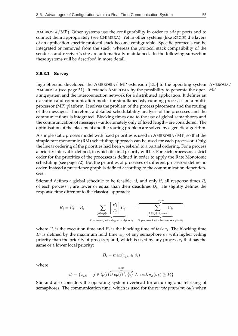
3.6. Advantages of Configuration within a Real-Time Communication System 55
AMBROSIA/MP). Other systems use the configurability in order to adapt ports and toconnect them appropriately (see CHIMERA). Yet in other systems (like REGIS) the layersof an application specific protocol stack become configurable. Specific protocols can beintegrated or removed from the stack, whereas the protocol stack compatibility of thesender’s and receiver’s site are automatically maintained. In the following subsectionthese systems will be described in more detail.
3.6.3.1 Survey
Ingo Stierand developed the AMBROSIA/ MP extension [135] to the operating system AMBROSIA/MPAMBROSIA (see page 51). It extends AMBROSIA by the possibility to generate the oper-
ating system and the interconnection network for a distributed application. It defines anexecution and communication model for simultaneously running processes on a multi-processor (MP) platform. It solves the problem of the process placement and the routingof the messages. Therefore, a detailed schedulability analysis of the processes and thecommunications is integrated. Blocking times due to the use of global semaphores andthe communication of messages –unfortunately only of fixed length– are considered. Theoptimisation of the placement and the routing problem are solved by a genetic algorithm.
A simple static process model with fixed priorities is used in AMBROSIA/MP, so that thesimple rate monotonic (RM) scheduling approach can be used for each processor. Only,the linear ordering of the priorities had been weekend to a partial ordering. For a processa priority interval is defined, in which its final priority will be. For each processor, a strictorder for the priorities of the processes is defined in order to apply the Rate Monotonicscheduling (see page 72). But the priorities of processes of different processors define noorder. Instead a precedence graph is defined according to the communication dependen-cies.
Stierand defines a global schedule to be feasible, if, and only if, all response times Riof each process τi are lower or equal than their deadlines Di. He slightly defines theresponse time different to the classical approach:
Ri = Ci +Bi +∑
j∈hp(i)
⌈RiTj
⌉Cj
︸ ︷︷ ︸∀ processes j with a higher local priority
+
new︷ ︸︸ ︷∑
k∈ep(i), k 6=iCk
︸ ︷︷ ︸∀ processes k with the same local priority
where Ci is the execution time and Bi is the blocking time of task τi. The blocking timeBi is defined by the maximum hold time zi,j of any semaphore σk with higher ceilingpriority than the priority of process τi and, which is used by any process τj that has thesame or a lower local priority:
Bi = max(zj,k ∈ βi)
where
βi = {zj,k | j ∈ lp(i)new︷ ︸︸ ︷
∪ ep(i) \ {i} ∧ ceiling(σk) ≥ Pi}Stierand also considers the operating system overhead for acquiring and releasing ofsemaphores. The communication time, which is used for the remote procedure calls when

56 Chapter 3. Configuration
global semaphores are used, is also considered:
Ci = CCOMPi +
∑
j
nLij(CL Pi + CL V
i )
︸ ︷︷ ︸use of local semaphores
+∑
k
nGik(CG Pik + CG V
ik )
︸ ︷︷ ︸use of global semaphores
CG Pik = CRPC IN + CSENDik + CL P
k + CSENDki + CRPC OUT
CG Vik = CRPC IN + CSENDik + CL V
k + CSENDki + CRPC OUT
For the analysis of the communications AMBROSIA/MP defines uni-directional commu-nication channels between two communicating processes. It is assumed, that all mes-sages over the channels have the same size. This restriction was made due to the fact thatAMBROSIA only supports communications via a CAN bus. CAN messages can containa maximum of 8 bytes. Outstanding is that AMBROSIA/MP handles communications,which have to be routed over several nodes (hops) when no direct link exists betweenthe nodes where the communication partners have been placed. It is also considered thatthe communication capacity (bandwidth) of a link is limited. For a successful routing ithas to be checked, whether no link is overloaded and all communication delays are lowerthan their defined maximum deadline: RSENDij ≤ DSEND
ij .
The modelling and implementation of the communication is made with buffers (mail-boxes) and dedicated communication processes that forward and receive the messagesover the communication links. There, all user processes, communication processes,buffers, and communication links are modelled as the nodes of a communication graph.Its edges define the communication paths and will be labeled with the required capaci-ties. The capacities and buffer sizes are determined during the optimisation phase. Forthe reservation of the bandwidth a special token protocol is implemented.
During the optimisation phase the mapping of the processes onto the processors and therouting of the messages over the communication links is determined. Additionally, thelocal priorities of the processes, the activation intervals of the communications for thetoken protocol and the required buffer sizes are calculated. The placement and routingproblem is defined by the DNA of a genetic algorithm. Therefore, Stierand also definesa quality function, which represents the quality of a solution. It is important for thegenetic algorithm that the quality function also ranks impossible solutions. For instance,the quality function will just give a negative value, when any deadline is not met. Theoverall quality function is the weighted sum of the three quality functions that rank theprocess mapping, the priority assignment and the routing.
After a feasible mapping and routing is found, the operating systems of each processornode in the system have to be configured. A configuration is described by the instanti-ation of components for the operating system in the AMScribe language. For each userand communication process a process component will be instantiated on the appropriatenode. For each message a routing component with the routing information as a param-eter is instantiated on every node, over which the message is routed. Additionally, onevery node some system components are instantiated, which represent all the systemcalls to the operating system. A system call can be the sending or receiving of a messageto or from a communication controller, as well as the acquiring or releasing of a localsemaphore. Whether a component must be instantiated or not, is simply evaluated overa logical existence term. For example, the code for the semaphore σi has to be integrated

3.6. Advantages of Configuration within a Real-Time Communication System 57
into the operating system for processor P , when there exists a process τi on P that uses σi.A component can also be instantiated more than once. The instantiation can be relativeto the amount of already installed objects of a concrete type. For instance, assume therealready exist four objects of type S1 and three objects of type S2 in the configuration. Thefollowing definition
COMPONENT C IF (EXISTSS1 and EXISTS S2) THEN PAR(a) END;
results into the integration of 12 instances of the component of type C, where the param-eter PARof all components will be set to a. This is done, because for all combinations ofinstances of the types in the condition the instantiation is made.
The automatic calculation of the process placement and the routing are two positive as-pects of AMBROSIA/MP. Limitations of AMBROSIA/MP are the fixed message size andthe use of a fixed communication protocol. Also, only four system calls, which are theacquire() and release() of a semaphore and the send() and receive() via aCAN controller, are handled by the analysis.
The CHIMERA Methodology [132, 133, 134] is a software engineering paradigm for the CHIMERA
implementation of real-time software for multi-sensor systems. It supports the devel-opment of dynamically reconfigurable component-based real-time software. CHIMERA
combines the port automaton theory with object-based (not object-oriented) design, whichresults in objects that are called port-based objects. These objects have input, output, andresource ports. Each object represents a single task. The communication between localinstances is done by connecting output ports to input ports. External communicationis done via resource ports, which access appropriate devices. The ports are named andonly such ports with identical names can be connected. A final configuration of all par-ticipated objects is legal, if, and only if, all input ports are connected to only one outputport. It is allowed to fan an output to multiple inputs. In CHIMERA exists join connectors(with the semantic of calculating the average) in order to combine several outputs to oneinput.
All communications in CHIMERA are done via a global state variables table. The port au-tomaton theory assumes that the most recent data is always present at the input ports.Message queues are not appropriate, because they accumulate the data in their queue andthe next data retrieved is not the most recent received one. So, connections of ports areimplemented by state variables. But reading or writing state variables by asynchronousparallel tasks cause integrity problems, which must be solved by using critical sectionsduring the access. These synchronisation mechanisms cause dependencies between theobjects. These dependencies are not allowed in the port-automaton model (autonomousexecution). Therefore, each port-based object gets its own copy of its referenced statevariables in a local state variables table. The key is to ensure that updates between bothtables are done only, when the task does not access its local table. Updates are done, whenthe task is not executing. This way, CHIMERA uses an inside-out method of programming,rather than the software invokes the operating system via system calls.
The CHIMERA real-time operating system provides tools to support the software mod-els defined by the CHIMERA methodology, so that real-time software can be executedpredictably using common real-time scheduling algorithms. The operating system ser-vices are always executing and invoke methods of the port-based objects. By this way,programmers have not to take into account communication and synchronisation. The

58 Chapter 3. Configuration
model assumes port-based objects can be in one of four states: NOT CREATED, OFF, ONand ERROR. The state transitions are results of signals, which are sent to the tasks, like:spawn , on , wakeup , off , re-init , kill , and clear . Each transition is done via callinga method of the object: init() , on() , cycle() , off() , kill() , error() , clear() ,re-init() , and sync() . Before and after each method call the table data are updated,distinguishing in/out constants and in/out variables. A two-step initialisation and ter-mination is used to support dynamic reconfiguration. High overhead initialisation andtermination code is performed during the init() and kill() methods, whereas taskscan be activated or suspended quickly using the on() and off() methods.
The tool suite DAVINCI [142, 147, 146] from Vector Informatik GmbH, Germany, supportsDAVINCI
the developer of distributed automotive applications. The Vector Informatik GmbH hasgreat knowledge and experience in this area and especially with tools for the design andanalysis of communication infrastructure and software for the CAN bus. DAVINCI seemsto be the most recent commercial development in the area of design and communicationsupport for distributed embedded control applications. DAVINCI supports the reuse ofcontrol software, the exchange of data via different networks, and the automatic designof the run-time environment for the distributed embedded control units. DAVINCI in-cludes a methodology for the developmnet of control applications. The development ofthe application software is based on the specification of software components. A softwarecomponent encapsulates the control algorithm, which can be specified in form of a finite-state-machine or in native C code. All information flow into the component and from thiscomponent is modelled by in/out signals. A software component is handled as a blackbox. The input and output signals can be connected with signals of the same type ofother components. Then the components form a network. Additionally, they can build ahierarchy. A component can consist of sub-components. Hereby, the signals of the super-component are redirected to the signals of its sub-components. A complete network ofsub-components can be integrated into a super-component.
In order to develop the overall functionality of an automotive software components haveto be assembled to a complete software application. Hereby, the components must ap-propriately be connected to each other. Still open signals have to connected to so-calledDevice Accessors. The device accessor represents an abstract sensor or actuator.
Before the complete code of the automotive application can be generated, the topologyof the hardware platform must be described. Hereby, the different available embeddedcontrol units are described together with the available actuators and sensors. Also theavailable communication busses between the controllers and sensors/actuators have tobe described. Actually, DAVINCI supports CAN and LIN.
In a third step of the applicaion development the software components have to bemapped onto the available embedded control units. This defines precisely which signalshave to transferred via messages over the buses and which signals can be exchanged byinter-process communication of the operating system. DAVINCI automatically incorpo-rates appropriate decice driver code for the communication buses, as well as appropriatesystem calls to the operating system. The priority of the messages and the transfer modesand protocols are automatically determined. Also the firmware in order to access the sen-sors and actuators is generated. It is worth to note that a sensor/actuator can be placedon another controller, as on which the software component is mapped, which uses thissensor/actuator.

3.7. Contribution of the Chapter 59
DAVINCI also automatically configures an OSEK compatible operating system for eachembedded control unit. DAVINCI incorporates a design methodology for closed dis-tributed control applications for automotives. It is the goal of DAVINCI to find and todefine reusable and sharable software components. The communication matrix of thecomponents will be automatically generated. The application specific code for each em-bedded control unit is also automatically generated. The bus communication and alsothe access to sensors and actuators is generated. The operating system of each embed-ded control unit is parameterized and configured in order to run the required tasks andcommunication drivers.
Thus, DAVINCI shares the ideas of the automatic code generation and the reusabilitywith TEReCS. However, the automatic check of the timing requirements of a real-timeapplication is not done. Nevertheless, DAVINCI embodies a variety of diagnostic inter-faces and functionalities, which allow to test the complete system or a component offlineon a PC or during run-time on the embedded control unit. But the configuration of theoperating and communication system is limited. The configuration aspect is far awayfrom the fine-grained approach that is used in TEReCS.
The REGIS system [100] is a distributed programming platform which adds protocol REGIS
stacks to communication endpoints. The system is more general and not only appli-cable to real-time applications. It uses standard transport layers (like UDP/IP or ATM)as the basis for data transportation. The basic (low-level) protocols and devices are stillmanaged by an operating system. Its key task is to describe a user-defined protocol stackby a graphical or textual representation. This is done in the language DARWIN. The basicidea is a strict hierarchical protocol stack through which data travel up- or downwards.Each layer has a well-defined interface. REGIS distinguishes between provision and re-quirement interfaces. Possible connections are only allowed between a provision and arequirement interface. By this means, REGIS defines services that have providing andrequiring dependencies between protocol layers. The system is implemented in object-oriented C++. One of the main advantages is the support for dynamic protocol stacks.Layers in the hierarchy can be introduced or removed during the lifetime of a connec-tion. This provides for dynamic binding of protocols during run-time. Predefined layersexist for sequencing, time-out, fragmentation, etc., resulting in the support for reliableprotocols. Code reuse is supported on the layer level.
3.7 Contribution of the Chapter
This chapter has characterised the problem which is solved by configuration. The con-figuration aspect is central to this thesis. Therefore, some of the advantages and disad-vantages of the existing approaches have been discussed. The different principles for theconfiguration have been introduced. This should help to select or adapt an appropriatealgorithm for the automatic configuration of operating systems and one communicationsystem. This chapter should also serve as a motivation for the idea that configuration isappropriate for the construction of such systems.

60 Chapter 3. Configuration

CHAPTER 4
Real-Time Analysis
. . . a sufficiently fast computer can satisfy the (timing) requirements,hence real-time computing is equal to fast computing. This is wrong.
John A. Stankovic, 1998 [125, p. 4]
Subject to this thesis is the configuration of embedded real-time operating and commu-nication systems. For this reason, “real-time” plays a crucial role for the correctness ofthe system. It is essential that the overall configuration process considers the real-timeaspect. This chapter will give a brief introduction into the theory of real-time analysis. Af-ter real-time is defined the basic approaches in the research for the analysis of the processscheduling are presented. The main goal that is handled by the schedulability analysisis the verification that all tasks will execute completely within a fixed and specified in-terval. Different assumptions about the task set’s properties lead to various algorithmsthat assure this timeliness execution. After the basic concepts of the process schedulingare presented the main approaches that have been transfered to the communication caseare briefly explained. For a nearly complete overview about this topic also the serverapproach for the process scheduling of sporadic tasks and the synchronisation problemsdue to resource access constraints are briefly described.
It should be mentioned that this chapter only presents the algorithms and achieved re-sults. The proofs for their correctness will not be given here. For these the interestedreader will be referred to the literature that is referenced in the appropriate sections.
4.1 Real-Time versus Non-Real-Time
Normal “visible” computers are equipped with an user interface (display, keyboard,mouse, joystick, touch-screen, etc.) and mainly run applications for the user’s sake. Of-ten, they present calculations or retrieval results or final layouts to the user according

62 Chapter 4. Real-Time Analysis
to some given inputs. In order to hold the response time for their reaction to the user’sinput as short as possible, their computing power has to scale accordingly to the prob-lem’s complexity. The performance of such computers is measured by the execution timein which they produce their results. In the case of serving multiple applications or userrequests in parallel (or semi-parallel) fairness and throughput become additionally im-portant. For all of these reasons a lot of resources are given to such computers (manyCPUs, high clock frequencies, huge memory, high speed communication adapters, etc.).
These characteristics become less important in the field of real-time computing. Real-timeapplications are mainly implemented for “embedded systems”. An embedded system typ-ically consists of a controlling system and a controlled system [125, p. 1]. Often, the con-trolling system is not visible. For example, the computers inside a washing machine orthe motor management for the engine inside an automobile are not directly visible to anuser of the controlled system. They are “embedded” into a technical system. Thus, thecontrolled system can be seen as the environment for the computer. The controlling sys-tem’s main purpose is the interaction with the controlled system. Thereby, it supportsthe controlled system in achieving its prime function.
The interaction of the controlling system with its environment is done by observing andmanipulating. Information is collected via several attached sensors. Upon this informa-tion a representation of the state of the environment is created inside the computer. Basedon this representation reactions to these, so-called stimuli, are calculated. These reactionsare manifested by generated output values, which are transmitted to the controlled sys-tem via actuators. Therefore, such a controlling system is also called reactive system.
Often, the phases of reading information, calculating reactions and writing output valuesis periodically done. Moreover, the controller is embedded into a closed loop, because itsoutput values have directly physical impact on the controlled system. Hence, the status ofthe controlled system normally changes and new input values have to be read. In orderto create correct control signals it is imperative that the state of the controlled system,as perceived by the sensors, is consistent with the actual state of the real environment.This implies that the internal time representation of the controlling system is equal to theexternal or “real” time of the environment.
Moreover, it is essential for real-time systems that their reactions take place within acertain time period or before a certain time limit expires. Thus, an upper time bound fortheir response time exists, which is called deadline.
Systems or applications can be distinguished in non-, soft-, firm- or hard-real-time systems.They are classified by the utility that the output values have. The generation time of anoutput value is thereby related to its deadline [25, p. 230-232]. In non-real-time systemsthe utility stays constant over the time. In a soft real-time system the utility function staysconstant until the deadline is reached. Then, it decreases linear to zero. That means, af-ter the deadline is reached, the results become more and more useless until they expiretotally. In a firm real-time system the utility function or usage of the values immediatelybecomes zero after the deadline is reached. In a hard real-time system the utility functiongoes immediately towards the negative infinity. This means that the profit or usage of thevalues turns into impairment, damages or defects of the controlled system and, maybe, ofits environment. Often, this means that catastrophic consequences can result from miss-ing a deadline. For instance, the system crashes or it seriously damages its environmentor even humans. In soft or firm systems it might be tolerable that a deadline is missed.

4.1. Real-Time versus Non-Real-Time 63
Typical examples for hard-real-time systems can be found in transportation vehicles likeautomobiles, trains, aircrafts and ships in their power-train control, engine control or insystems like steer-by-wire and brake-by-wire. Mostly, malfunctions of these systems ob-viously lead to severe problems, which are menacing even human’s lives. A malfunctionin real-time systems happens, when an actuator is not set in its predefined time windowaccordingly to the required value due to timing problems in the calculation path.
The weather forecast or the decision on stock exchange orders can be seen as firm-real-time systems. If their results are produced too late, then their usage might be worthnothing. Moreover, it is widely accepted that this can happen, respectively that theirresults can be wrong.
In the field of transmitting real-time video or audio data soft deadlines are defined. If thedata are received too late, then the display or their play back might be disturbed. Thisresults into jitters or artificial artifacts. But nevertheless, the information that is containedin the stream is transmitted. Only the quality of the stream might be decreased. In thiscontext the term Quality of Service (QoS) is often used in order to specify the probability orthe estimated average amount of probably missed deadlines (and its standard deviationand related values).
It is the primary goal of real-time systems that all tasks meet their deadlines. And itshould be mentioned clearly, that the fact how fast they execute is (nearly) of no interest;but that they will never reach the deadline! Ditze [42, p. 10] stated:
“Timeliness is the dominating QoS requirement here, which fundamentally differsfrom the aim of HPC applications. Performance and fairness properties are regardedless important.”
Buttazzo summarizes the basic properties that real-time systems must have to supportcritical applications [25, p. 12]:
Timeliness. Results have to be correct not only in their value but also in the time do-main.
Design for peak load. Real-time systems must not collapse when they are subject topeak load conditions, so they must be designed to manage all anticipated scenarios.
Predictability. To guarantee a minimum level of performance, the system must be ableto predict the consequences of any scheduling decision. If some task cannot beguaranteed within its time constraints, the system must notify this fact in advance,so that alternative actions can be planned in time to cope with the event.
Fault tolerance. Single hardware and software failures should not cause the system tocrash. Therefore, critical components of the real-time system have to be designedfault tolerant.
Maintainability. The architecture of a real-time system should be designed accordingto a modular structure to ensure that possible system modifications are easy to per-form.
In order to achieve the timeliness, hard real-time systems are designed under the as-sumption that everything is known what can happen and when it happens. This means
64 Chapter 4. Real-Time Analysis
everything is predictable. In fact, that all tasks will meet their deadlines under theseassumptions, will be predicted (verified or falsified). More in detail, this is done by aso-called formal real-time analysis. In the past decades a lot of research have been done inthis field. Because the configurator, which had been developed in this thesis, deals withreal-time communication, also a simple real-time analysis approach has been integratedinto TEReCS (see page 133). For this reason in this chapter some basic and importantresearch results for the real-time analysis will briefly be presented.
The request for maintainability of a real-time system can easily be handled by configu-ration. Configuration is an appropriate way in order to maintain all options of a cus-tomisable system. But configuration and real-time analysis must be integrated. Boththey cannot be seen isolated. Real-time analysis should steer the configuration or theconfiguration must qualify its solution by an analysis. This is ensured in TEReCS (seeSection 6.9142 and Section 6.10147).
4.1.1 Definition of Real-Time System
Because the configuration of a real-time system is the main topic of this thesis, a definitionof a real-time system will be given. In order to clarify the sketched picture of the previoussection a few definitions from researchers of the real-time community are presented here.Often Young is cited, who defined a real-time system as
“ . . . any information processing activity or system which has to respond to externallygenerated stimuli within a finite and specified period.” S. Young, 1982 [150]
A quite similar definition had been provided later by Randell:
“A real-time system is a system that is required to react to stimuli from the environ-ment (including the passage of physical time) within time intervals dictated by theenvironment.” B. Randell, 1995 [105]
These two definitions define a real-time system by its reactions to external stimuli and– that is important – by the definition of a time bound (deadline), which defines whenthis reaction has to take place after their appearance. Stankovic [122] and Kopetz got theheart of these properties:
“A real-time computer system is a computer system in which the correctness ofthe system behaviour depends not only on the logical results of the computations,but also on the physical instant (deadline) at which these results are produced. ”Hermann Kopetz, 1997 [72]
It should again be realised that the timeliness is an essential property of real-time systems.Moreover, the system’s behaviour might be incorrect, if some deadlines are missed. Be-cause timing faults may cause severe damages or injuries, the correctness of a real-timesystem must be guaranteed. The deadlines define timing constraints, that the system mustsatisfy. The correctness is formally verified by a so-called schedulability test. This testchecks, whether for all possible execution orders of the system’s processes and threadsthe reactions will be before their deadlines. This test can only be done, if the worst-case

4.2. Real-Time Analysis for Process Scheduling 65
execution time of the processes and threads, their communication delay and their resourceand precedence constraints are known in advance (are predictable). Resource constraintsarise because of mutual exclusion and precedence constraints arise because of output-to-input dependencies. Normally, this test is done for static systems (i.e. changes of theseassumptions do not occur during execution) before their run-time (offline). If these as-sumptions change during execution, because new processes have to be started or theirexecution time or their resource and precedence constraints change, then this system isknown to be dynamic. Then, the so-called acceptance test for new processes or constraintshas to be done during run-time (online).
An overview about these schedulability and acceptance test will be given in Section 4.2and Section 4.476.
4.2 Real-Time Analysis for Process Scheduling
In the past decades excellent results are produced in the area of real-time analysis for pro-cess scheduling. Due to the fact that the configuration developed in this thesis also dealswith a complete customisable operating system and a lot of the results can –more or less–directly applied to real-time communication, some of the basic and most important re-sults will shortly be introduced in this chapter.
For predictable real-time systems, i.e. all of its properties are well known, various algorithmshad been developed in order to proof formally whether all tasks will meet their deadlinesunder all circumstances. In detail this means that each process of the system will termi-nate before its deadline. Therefore, the order of execution of each task is constrained in acertain manner by the task scheduler. Nevertheless, a lot of remaining possible executionorders exists. It is the task of a so-called schedulability test to verify or falsify upon thegiven properties and constraints, if a concrete and given set of processes will meet theirdeadlines or not. Input to this test are the task set and all of the system’s properties. Thetest will mostly be done offline before the system is implemented. But if the system’sproperties will change during run-time or the task set will change, then the test must bedone online during execution in order to allow the change or not. Only if changes donot lead to deadline misses, they can be accepted. Thus, the online test is often calledacceptance test.
As previously mentioned the execution order of the tasks is constrained. That meansthat the scheduling of the task set underlies some restrictions. For this reason a variety ofscheduling algorithms had been developed. The scheduling algorithm and its schedula-bility test should guarantee the timeliness execution of a given task set (feasible schedule).This must formally be proofed. An algorithm and its schedulability test are only cor-rect, if under all circumstances and for all possible task sets a feasible schedule will beexecuted when the schedulability test accepts the task set.
This means that real-time analysis defines proofs on two levels: On the higher level thescheduling algorithm and its schedulability test must be verified and on the second levelthe formal schedulability or acceptance test is identifying only valid task sets. A schedul-ing algorithm and its schedulability test are called to be optimal, if they accept the taskset when there exist at least one valid schedule so that all deadlines are met and thescheduler will execute this schedule.

66 Chapter 4. Real-Time Analysis
4.2.1 Definitions
Before some analysis approaches for real-time systems will briefly be presented, we willgive some definitions of characteristics and parameters of a real-time computing sys-tem. Most of these are timing constraints or properties because timeliness is the cru-cial characteristic of a real-time system. Processes or tasks are the basic items, whichcarry out the calculation paths of the implemented algorithms. Therefore, a set of tasksΓ = {τi | i = 1, 2, . . . , n} is identified to be subject of the analysis.
The following properties of a task τi are of interest for the real-time analysis:
• Arrival time ai: is the time at which the task becomes ready for execution; it is alsoreferred as request time or release time indicated by ri.
• Computation time Ci: is the time necessary to the processor for executing the taskwithout preemption. The worst case execution time of a task is denoted by WCET .
• Deadline Di: is the time before a task should be completed.
• Start time si: is the time at which the task starts execution.
• Finishing time fi: is the time at which the task finishes execution.
• Response timeRi: Ri = fi−ri is the time, measured from the release time, at whichthe task is finishing.
• Lateness Li: Li = fi − di represents the delay of a task completion with respectto its deadline. Note, that if a task completes before its deadline, its lateness isnegative. Often scheduling algorithms try to minimize the lateness of each task orthe maximum lateness Lmax of all tasks.
• Tardiness or Exceeding timeEi: Ei = max(0, Li) is the time a task stays active afterits deadline.
• Laxity or Slack time Xi: Xi = di − ai − Ci is the maximum time a task can bedelayed on its activation to complete within its deadline.
In general, a task set can consist of tasks with different characteristics. Often, for theanalysis only specific characteristic are allowed in order to simplify the implementationor the analysis itself. A task set can be classified by
Periodic or aperiodic tasks. The instances of a periodic task τi are regularly activated ata constant rate. The interval Ti between two consecutive activations is the periodof the task. A periodic task set consists only of periodic tasks. An algorithm thatis implemented only (!) of periodic tasks is often called to be time-driven (see Sec-tion 4.4.2.384). If there exists aperiodic tasks or interrupts (a special kind of a low-level aperiodic task), then the system is modelled event-driven. Periodic tasks areactivated synchronously while aperiodic tasks have an asynchronous activation.
Independent tasks or tasks with resource or precedence constraints. Precedence con-straints arise because of output-to-input dependencies between the tasks. Thatmeans that a task τi cannot run before task τj , because τj produces an output, which

4.2. Real-Time Analysis for Process Scheduling 67
is required as input for task τi. All dependencies of such a kind can be modelled ina directed precedence graph. Resource constraints occur when tasks must have exclu-sive access to resources, because they have to run critical sections in order to protectthe integrity of the resource. The mutual exclusion let tasks block other tasks so thatthey cannot proceed with their calculations. If this happens, a task switch have tobe done, which has direct implications onto the schedule. If there exists no resourceor precedence constraints, then the tasks are said to be independent.
Preemptive or non-preemptive execution. A task τi can be assigned a priority pi. Ahigher priority of a ready task means that the task must be executed before all otherlower-priority tasks that are ready. This implies that if a higher-priority task be-comes ready while a lower-priority task is actually executed, then the lower-prioritytask must be suspended and the execution of the higher-priority task must imme-diately be continued. This fact is known as preemption. (In non-priority systemspreemption often denotes the fact that a task is suspended because its time sliceof being executed is expired. Then the next task is executed by a so-called Round-Robin scheme.)
Static or dynamic priority assignments. The priorities of the tasks can be assigned stat-ically so that they never change during the run-time of the system or they can bemodified while execution and are therefore dynamic.
Soft, firm or hard real-time tasks. The criticalness is a parameter related to the conse-quences of missing a deadline (see page 62).
Deadline or period driven analysis. The deadlines define a border for the maximum ex-ecution time of a task. Thus, the deadline relative to the last task activation mustobviously not be greater than the period of the task. But they can be identical. Ifthey are equal, then the analysis identifies the periods with the deadlines. Underthis assumption it is often enough to analyse the processor utilisation. Otherwise,the response time or processor demand have to be analysed (see Table 4.274).
For a periodic task set the hyperperiod H can be defined as the least common multiple of theperiods of all tasks. This is important, because the execution order of all tasks (which isnamed schedule) will obviously be repeated after a multiple of H .
These additional assumptions are often made for periodic tasks:
• All instances of a periodic task have the same worst case execution time Ci.
• All instances of a periodic task have the same deadline di relative to the beginningof a period.
For a periodic task τi the phase Φi can be defined as the release time of the first instanceof the task. The task identifier τi,j , the release time ri,j , the absolute deadline di,j =Φi + (j − 1)Ti + di, the start time si,j , and the finishing time fi,j are sometimes suppliedwith an additional index j denoting the jth instance.
Very important for real-time systems is often the so-called absolute release jitter ARJi =maxj(si,j − ri,j) −minj(si,j − ri,j). It is the maximum deviation of the start time amongall instances. The absolute finishing jitter AFJi = maxj(fi,j − ri,j)−minj(fi,j − ri,j) is the
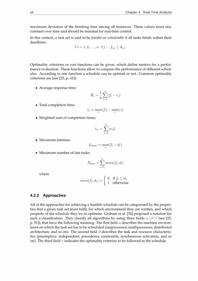
68 Chapter 4. Real-Time Analysis
maximum deviation of the finishing time among all instances. These values must stayconstant over time and should be minimal for real-time control.
In this context, a task set is said to be feasible or schedulable if all tasks finish within theirdeadlines:
∀ i = 1, 2, . . . , n ∀ j : fi,j ≤ di,j .
Optimality criterions or cost functions can be given, which define metrics for a perfor-mance evaluation. These functions allow to compare the performance of different sched-ules. According to one function a schedule can be optimal or not. Common optimalitycriterions are (see [25, p. 41]):
• Average response time:
Ri =1n
n∑
i=1
(fi − ri)
• Total completion time:tc = max
i(fi)−min
i(ri)
• Weighted sum of completion times:
tw =n∑
i=1
wifi
• Maximum lateness:Lmax = max
i(fi − di)
• Maximum number of late tasks:
Nlate =n∑
i=1
miss(fi, di)
where
miss(fi, di) =
{0 if fi ≤ di1 otherwise
4.2.2 Approaches
All of the approaches for achieving a feasible schedule can be categorised by the proper-ties that a given task set must fulfil, for which environment they are written, and whichproperty of the schedule they try to optimise. Graham et al. [54] proposed a notation forsuch a classification. They classify all algorithms by using three fields α β γ (see [25,p. 51]), that have the following meaning: The first field α describes the machine environ-ment on which the task set has to be scheduled (uniprocessor, multiprocessor, distributedarchitecture, and so on). The second field β describes the task and resource characteris-tics (preemptive, independent, precedence constraints, synchronous activation, and soon). The third field γ indicates the optimality criterion to be followed in the schedule.

4.2. Real-Time Analysis for Process Scheduling 69
In the following paragraphs the most important scheduling algorithms for real-time sys-tems are presented. Only the basic idea of the algorithm and a motivation for its correct-ness will be given. For details and formal proofs we would like to refer to the literatureand especially to the book “Hard Real-Time Computing Systems” from Buttazzo [25].
In general, the algorithms can be classified by the prerequisites, which they demand.The algorithms can primarily be classified whether they can handle periodic or aperi-odic tasks. The first section describes algorithms for aperiodic tasks, the second sectionalgorithms for periodic tasks.
4.2.2.1 Aperiodic Task Sets
Earliest Due Date (EDD). This algorithm is also known as Jackson’s Algorithm. Alltasks for this algorithm have to arrive synchronously, that means at the same time, andrun only once, but can have different execution times and deadlines. Neither they musthave precedence constraints, nor they must use resources in exclusive mode. It is alsoassumed that all tasks must run on a single processor. The algorithm proposed by Jack-son [68] minimizes the maximum lateness. (Graham’s class: 1 sync Lmax)
By EDD the tasks have to be executed in the order of increasing deadlines. For proofingthe correctness assume that exchanging the order of two consecutive tasks in any sched-ule will not increase the maximum lateness of the complete schedule. But the maximumlateness of these two tasks will be smaller if they are ordered appropriately.
Earliest Deadline First (EDF). This algorithm had been proposed by Horn [63] and han-dles tasks with arbitrary arrival times. This is especially the case when tasks arrive dy-namically during execution of other tasks. It is very easy to find a feasible schedule, ifpreemption is allowed. That means that the actual task can be suspended in order to exe-cute a more important task. A feasible schedule and minimizing the maximum latenesscan be achieved if always the task with the earliest deadline is executed. Dertouzos [37]showed that EDF is optimal in the sense of feasibility. (If there exists a feasible schedule,then it will be found. Graham’s class: 1 asynch → preem Lmax → feasible) In fact, analgorithm that minimizes the maximum lateness is also optimal in the sense of feasibility.The contrary is not true.
The acceptance test for a task must certify that for all tasks its worst case finishing timefi is before its deadline di. The worst case dynamic finishing time of task τi is equal tothe sum of the worst case dynamic finishing time of task τi−1 with next lower deadlineand the remaining worst case execution time ci(t) of task τi. (Thus, all tasks τi are alwaysordered by increasing deadline: di < dj ⇔ i < j.) Notice, that ci(t) has an initial valueequal to its computation time Ci and can be updated whenever the task τi is preempted.
∀ i = 1, . . . , n : fi = fi−1 + ci(t) =i∑
k=1
ck(t) ≤ di
Tree search. If the tasks arrive asynchronously but preemption is not allowed, then EDFis no longer optimal. The problem of minimizing the maximum lateness and the problemof finding a feasible schedule become NP-hard [71, 82, 83]. For this category branch-and-bound algorithms search in all possible schedules for a feasible schedule. They performwell in the average case but degrade to exponential complexity in the worst case. The

70 Chapter 4. Real-Time Analysis
structure of the search space is a tree, where in each level a new task is introduced intothe schedule. This results to a tree depth on n for n tasks and a tree with n! (n factorial)leaves. The branch-and-bound technique proposed by Bratley et al. [20] stops searchinga path from the root to a leave, when adding a task to the actual schedule will lead toa missed deadline. This reduces dramatically the search space but the algorithm has inworst case still a complexity of O(n n!). (Graham’s class: 1 no preem feasible)
Spring. This algorithm had been created for the SPRING kernel [123, 124] designed atthe University of Massachusetts by Stankovic and Ramamritham. The algorithm belongsalso to the tree search algorithms, but it uses a heuristic function in order to determinethe task for extending the schedule. Thereby, only one path of the tree is evaluated, butfor each extension of the schedule the heuristic function have to be evaluated for all tasks.Thus, the complexity reduces to O(n2), but it is not guaranteed that the algorithm willfind the feasible schedule if it exists (it is not optimal in finding).
The heuristic function in Spring can be set to the minimal arrival time (resulting intoscheduling after First Come First Served), the computation time (resulting into schedul-ing after Shortest Job First) or the deadline (resulting into scheduling after EDF). In orderto handle additionally tasks with exclusively used resources the heuristic function can beset to the minimum estimated starting time Test(i). Test is the maximum of the arrival timeand all of its earliest available resource times (EAT ) for all of its required resources. EATfor a resource k is determined upon the already defined partial schedule. Additionally, inSpring precedence constraints can be considered. Thus, the heuristic function only selectsa task, when all of its predecessors are already scheduled and executed.
Latest Deadline First (LDF). If the given task set has also precedence constraints, i.e.tasks must be executed before other tasks, then it becomes more difficult to find a fea-sible schedule. In general the problem becomes also NP-hard. But if we can assume thatall tasks arrive at the same time (synchronously), then Lawler [76] found the algorithmcalled Latest Deadline First also to be optimal in minimizing the maximum lateness (Gra-ham’s class: 1 prec, sync Lmax) and it can be computed in O(n2) time. LDF builds theschedule from the tail to the head. Among all tasks with no successors or whose suc-cessors have already been all selected, LDF selects the task with the latest deadline to bescheduled last. That means at run-time the task which is inserted last into the schedulewill be executed first. The proof for the correctness is done similar to the one for the EDDalgorithm.
EDF∗. Chetto, Silly and Bouchentouf [27] found a very elegant way to schedule a taskset with precedence constraints with a modified EDF algorithm. Thus, the task set mustbe preemptable (Graham’s class: 1 prec, preem Lmax). Their idea is to transform thedependent task set into an independent task set by modifying the timing constraints.In fact, if the timing constraints are met, then it must follow that also the precedenceconstraints must by obeyed. In detail the minimal start time (or release time) and thedeadline for the tasks have to be modified. Assume, that task τi must precede task τj ,then the start time of τj must not be before the end time of τi: rj = max(rj , ri + Ci).Additionally, the task τi must finish before task τj . This can be achieved by modifyingthe deadline of τi: di = min(di, dj − Cj). These modifications can both be computed inO(n2) time. (The precedence graph must be traversed appropriately and for each taskthe maximum, respectively minimum must be found.)

4.2. Real-Time Analysis for Process Scheduling 71
For aperiodic task sets various algorithms had been given which are applicable under dif-ferent terms of assumptions on the task set (synchronous, preemptive, precedence con-straints). The algorithms also differ in their computational complexity. A summary ofthese algorithms can be found in Table 4.1.
sync. activationpreemptive
async. activationnon-preemptiveasync. activation
EDD(Jackson ’55)
EDF(Horn ’74)
Tree search(Bratley ’71)
independent O(n log n) O(n2) O(n n!)
Optimal Optimal Optimal
LDF(Lawler ’73)
EDF∗
(Chetto et al. ’90)
Spring(Stankovic &
Ramamritham ’87)precedenceconstraints
O(n2) O(n2) O(n2)
Optimal Optimal Heuristic
Tab. 4.1: Scheduling algorithms for aperiodic tasks. (see [25, p. 75])
4.2.2.2 Periodic Task Sets
The basis for the schedulability test in the periodic case is the processor utilisation factor U .Since Ci/Ti is the fraction of the processor time spent in executing task τi, the utilisationfactor for n tasks as originally given by Liu and Layland in 1973 is defined by the equation
U =n∑
i=1
CiTi
[85].
Obviously, any task set that has an utilisation factor greater than one is infeasible, becausethe utilisation factor is a measure of the computational load of the processor and that can-not exceed 100%. On the other hand for each task set Γ and for each scheduling algorithmA exists another upper bound Uub (0 < Uub ≤ 1) for which the task set is schedulable andany increase in the utilisation of any task will make the schedule infeasible. With suchan Uub(Γ, A) the set Γ is said to fully utilise the processor. For a given scheduling algo-rithm A, the least upper bound Ulub(A) of the processor utilisation factor is defined as theminimum of all Uub(Γ, A) for all task sets Γ, which fully utilise the processor.
That means that a task set Γ is certainly feasibly schedulable if its processor utilisationfactor is below the least upper bound [U(Γ, A) ≤ Ulub(A)], but it need not to be schedu-lable if it is greater as the least upper bound [Ulub(A) < U(Γ, A) ≤ 1], and it is absolutelynot schedulable if it is greater than one [U(Γ, A) > 1].
Various algorithms had been defined for different assumptions made for the task set.Each algorithm A defines its own least upper bound Ulub(A). In the following the most

72 Chapter 4. Real-Time Analysis
important and widely used algorithms for aperiodic task scheduling will be shortly pre-sented.
Rate Monotonic (RM). This algorithm assigns priorities to the tasks. Thereby, tasks withshorter periods will be given higher priorities. Since periods are constant, RM assigns thepriorities statically before run-time and the priorities will never change. RM is intrinsi-cally preemptive. Thus, an actually running task is preempted by a newly arriving taskwith shorter period. In 1973, Liu and Layland [85] showed that RM is optimal among allfixed-priority algorithms. That means that no other fixed-priority algorithm can feasiblyschedule a task set, which cannot be scheduled by RM. They also derived the least upperbound for the processor utilisation factor. A generic task set of n tasks has
Ulub(Γn, RM) = n(21/n − 1).
For any task set with an unlimited amount of tasks this is often also given as
Ulub(Γ, RM) = limn→∞n(21/n − 1) = ln 2.
A detailed derivation of this can be –of course– found in [85] and in [25, p. 82]. It shouldclearly be mentioned here, that this schedulability condition is sufficient to guarantee thefeasibility of a task set, but it is not necessary. That is, if the utilisation factor is betweenUlub and 1, then nothing can be said about the feasibility of the set. However, since RMis optimal an improvement can only be achieved by using dynamic-priority assignmentalgorithms.
Earliest Deadline First (EDF). The EDF algorithm –as already presented in Sec-tion 4.2.2.169– is also applicable for periodic tasks. EDF selects tasks according to their ab-solute deadline, which means that the task with an earlier deadline will be executed first.Thus, the priority will be assigned dynamically during execution to the tasks. Thereby,EDF is intrinsically preemptive. The optimality criterion also holds for periodic tasks.Moreover, EDF can be used to schedule aperiodic and periodic tasks at the same time.Based on the results achieved by Liu and Layland [85], Spuri, Buttazzo, and Sensinishowed in [119] and [25, p. 93] that the least upper bound for the processor utilisationfactor under EDF is one:
Ulub(Γn, EDF ) = 1.
Deadline Monotonic (DM). The Deadline Monotonic priority assignment algorithmweakens the “period equals deadline” constraint. Each task τi of the task set may havean arbitrary deadline Di ≤ Ti. But Di stays constant for all instances of τi. According tothe DM algorithm, each task is assigned a priority inversely proportional to its deadline.Since deadlines are constant, DM is also a fixed-priority assignment algorithm. In 1982,Leung and Whitehead [84] proposed this algorithm as an extension for the RM. Theyshowed in a similar way compared to RM, that DM is also optimal for fixed-priorities anddeadlines lower than their periods. The sufficient schedulability test for RM can be ap-plied for DM, if the periods are replaced by their deadlines:
∑ni=1(Ci/Di) ≤ n(21/n− 1).
However, such a test is not optimal as the workload on the processor is overestimated.A less pessimistic and also sufficient schedulability test calculates the maximum inter-ference Ii of higher priority tasks on the lower priority task τi. Assuming that the tasksare ordered by increasing relative deadlines (i < j ⇔ Di < Dj), then this interference

4.2. Real-Time Analysis for Process Scheduling 73
is Ii =∑i−1j=1dDi/Tje Cj . The schedulability test has to assure for all tasks that the fin-
ishing time is before the deadline: ∀i : 1 ≤ i ≤ n Ri = Ci + Ii ≤ Di. This testassures that a higher prioritised task τj interferes task τi in every of its periods Tj . Butthis might not be true, if the execution time of task τi is so small, that its finishing time orresponse time Ri < (dDi/Tje − 1)Tj . That means, if at least in the last period of τj , whichcovers the deadline of τi, task τj does not interfere (preempt) τi, then the interference isoverestimated. That means that also this test is only sufficient but not necessary.
In 1992/1993, Audsley et al. [5, 4] proposed a sufficient and necessary schedulability testfor DM. They propose to use the response time Ri of task τi instead its deadline Di forthe calculation of the number of interferences. Thus the equation, which is to be checkedfor all tasks is
∀i : 1 ≤ i ≤ n Ri = Ci + Ii = Ci +i−1∑
j=1
⌈RiTj
⌉Cj ≤ Di.
The problem in calculating the response time is that Ri appears on both sides of theequation. Fortunately, Ri can be computed stepwise from the first to the last interference[25, p. 101]:
schedulability test(DM) :=
R0i = Ci, I
−1i = 0
do
Rk+1i = Iki + Ci with Iki =
∑i−1j=1
⌈RkiTj
⌉Cj
until Ik+1i + Ci ≥ Rk+1
i
Rk+1i ≤ Di ⇔ feasibility
Moreover, in the calculation of this recurrent formula the task set is not feasible, if ∃ k :Rki > Di.
EDF∗. Also EDF with its dynamic-priority assignment approach is again applicable toperiodic task scheduling when deadlines are less to periods. Only the schedulability testhas to be adapted. Baruah, Rosier, and Howell [8] proposed in 1990 to use the processordemand criterion. The processor demand of any task set during the interval [0, L] is definedas the cumulative processing time CP (0, L) that is required by tasks with deadlines lessor equal to L: CP (0, L) =
∑ni=1bL/TicCi. In 1993, Jeffay and Stone [69] stated that a set of
periodic tasks with deadlines equal to periods is schedulable under EDF, if and only if
∀L ≥ 0 : L ≥n∑
i=1
⌊L
Ti
⌋Ci.
It should be noticed that it suffices to test the equation only for values ofL equal to releasetimes less than the hyperperiod H , because ∀L ∈ [rk, rk+1), bL/Tic = brk/Tic. Moreover,it is enough to test the equation for values of L for release times less or equal to the busyperiodBP = min{L W (L) = L}withW (L) =
∑ni=1dL/TieCi. During the busy period the
processor is fully utilised. It ends either with an idle time, or with the start of a release ofa new periodic instance.
Baruah, Rosier, and Howell [8] showed that for periodic tasks with deadlines less thanperiods the processor demand can still be used, if considered that the last interval cov-ering L must be taken into account, if the deadline is before L (Di ≤ L, see Figure 4.1).

74 Chapter 4. Real-Time Analysis
L0
J1
J2
Fig. 4.1: Processor demand when deadlines are less than periods (from [25, p. 106]).
Thus, if D = {di,k di,k = kTi + Di, di,k ≤ min(BP ,H), 1 ≤ i ≤ n, k ≥ 1}, then a set ofperiodic tasks with deadlines less than periods is schedulable by EDF if and only if
∀L ∈ D L ≥n∑
i=1
(⌊L−Di
Ti
⌋+ 1
)Ci.
A summary of scheduling algorithms for periodic tasks can be found in Table 4.2. No-tice, that the algorithms for deadlines equal to periods can be solved by the processorutilisation approach and therefore, they can be computed in linear time (O(n)), whereasthe processor demand approach for task sets with deadlines less than periods requirespseudo-polynomial time.
Di = Ti Di ≤ Ti
RM DM
Staticpriority Processor utilisation approach Response time approach
U ≤ n (21/n − 1) ∀ i : Ri = Ci +i−1∑j=1
⌈RiTj
⌉Cj ≤ Di
EDF EDF∗
Dynamicpriority Processor utilisation approach Processor demand approach
U ≤ 1 ∀L ≥ 0 L ≥n∑i=1
(⌊L−DiTi
⌋+ 1
)Ci
Tab. 4.2: Summary of guarantee tests for periodic tasks. (see [25, p. 107])
4.3 Servers for Aperiodic Tasks
In most real-time applications periodic and aperiodic tasks have to be executed in parallel(or quasi-parallel). Typically, the periodic tasks are time-driven and underlie hard real-time constraints, whereas the aperiodic tasks are event-driven and have soft or firm andrarely hard real-time constraints. The main objective of the real-time operating system is

4.3. Servers for Aperiodic Tasks 75
to guarantee the hard real-time tasks and to provide a good average response time andminimal deadline misses for soft and firm real-time tasks.
Often, aperiodic tasks are characterised by a minimum inter-arrival time, which definesa kind of maximum probable period. For this reason they are also called sporadic tasks.In the scheduling theory aperiodic tasks are handled in another way than periodic tasks.Whereas in the previous sections some basic techniques for hard real-time scheduling hadbeen discussed, in this section some principles for real-time scheduling with combinedperiodic and aperiodic task sets will be presented.
The so-called server technique is an appropriate approach to handle aperiodic real-timetasks in the case when a periodic scenario is assumed. A specific periodic task is re-sponsible to service all pending aperiodic requests. This special task is called server. Theserver approach tries to optimise the processor utilisation bound and tries to minimizethe response time for aperiodic requests in contrast to non-server techniques.
Background Scheduling. In Background Scheduling soft aperiodic tasks are handled inthe background behind periodic tasks. They will be executed after all hard real-timetasks had run and still some processor time is left. Therefore, aperiodic real-time taskswill get assigned a priority just lower than the priority of any periodic real-time task.
Fixed Priority Servers. A representative for a Fixed Priority Server is the so-called PollingServer (PS). The server task has (as any periodic task) a period Ts and a maximum com-putation time Cs. The computation time is called capacity of the server. The server isscheduled like any other periodic real-time task, not necessarily at lowest priority. Theschedulability test for a combination of PS under RM can be guaranteed if
Up + Us =n∑
i=1
CiTi
+CsTs≤ Ulub(n+ 1) = (n+ 1)(21/(n+1) − 1) .
The finishing time fa of an aperiodic request τa = (ra, Ca, Da) can be computed as
fa =⌈raTs
⌉Ts +
⌊CaCs
⌋Ts + (Ca −
⌊CaCs
⌋Cs) .
This results into a schedulability test for aperiodic tasks: fa ≤ ra +Da [25, p. 111 ff.].
Another Fixed Priority Server is the Deferrable Server (DS) proposed by Lehoczky, Sha, andStrosnider [79, 136]. Unlike the Polling Server, DS preserves its capacity until the end ofits period. Only, when aperiodic tasks are served, the capacity is decreased accordingly.With the beginning of each server’s period, the capacity is replenished at its full value.Thus, future aperiodic requests can be served until the capacity is exhausted during thewhole period of the server. The schedulability test for a combination of DS under RM canbe guaranteed if
Up ≤ ln(Us + 22Us + 1
).
Note, that if Us < 0.4 Up, then the RM bound (ln 2) gets worser, but for Us ≥ 0.4 thepresence of DS improves the Ulub(DS) = Us+ln( Us+2
2Us+1) (see [25, p. 119 ff.]). The finishingtime of an aperiodic request under DS can be computed to
fa =
{ra + Ca if Ca ≤ cs(t)⌈raTs
⌉Ts +
⌊Ca−∆aCs
⌋Ts + (Ca −∆a −
⌊Ca−∆aCs
⌋Cs) otherwise,

76 Chapter 4. Real-Time Analysis
where ∆a = min[cs(t), (⌈raTs
⌉Ts − ra)] [25, p. 116 ff.].
Priority Exchange Server. The Priority Exchange Server (PE) had been introduced in 1987,by Lehoczky, Sha, and Strosnider [79]. The PE algorithm also uses a periodic servertask (usually at a high priority) for servicing aperiodic requests. The capacity of theserver is not preserved at the server’s priority while no aperiodic request are pending.However, the capacity is divided into capacities on all priority levels. At the beginningof the server’s period its capacity is replenished at its full value. If no aperiodic requestsare pending and a periodic task have to be executed, then the capacity is borrowed ortransfered to the capacity of the periodic task’s level. Otherwise, (that means an aperiodicrequest can be executed, due to having capacity on any level, or the processor is idle) thecapacity degrades linear from level to level. By this, the server’s priority is virtuallyexchanged with a scheduled periodic task. By this rule, the capacity is preserved at theperiodic task’s priority level and can be consumed later if required. The capacity is onlyconsumed by idle times or serving aperiodic requests. The least upper bound for theprocessor utilisation factor, when PE is combined with RM for the periodic tasks, is
Up ≤ ln(
2Us + 1
)[25, p. 125 ff.].
Other examples for servers are the Sporadic Server (SS) [116] and the Slack Stealing Method[81]. Appropriate adaptations of all these Fixed Priority Servers to the dynamic case,where the periodic tasks are scheduled using EDF, are made by Buttazzo et al. [117, 118].The Dynamic Priority Servers are the Dynamic Priority Exchange Server (DPE), the DynamicSporadic Server (DSS), the Total Bandwidth Server (TBS) and the Earliest Deadline Late Server(EDL).
4.4 Real-Time Analysis for Communication
When we have a distributed system, tasks run on different processors. They often com-municate via communications links. Tasks will send and receive data from other tasks.This defines in/out dependencies between the tasks. These in/out dependencies can bemodelled by precedence constraints. But, in fact, a receiving task can execute until it re-quires input from another task. If this input is not present, the task will be blocked. Thisis the normal case. It is also possible that the receiving task continues execution, althoughinput data are not present. This is called asynchronous receive, whereas the normal one iscalled synchronous receive. Also the sending of data can be asynchronous or synchronous.Here, the normal case is the asynchronous case, where the sender task continues with itsexecution directly after the data are sent. In the synchronous case the sender task willbe blocked until the receiver task has received the data. Therefore, an acknowledgementhas to be sent back. The synchronous send and the synchronous receive define a so-calledrendezvous.
Because the synchronous send and the asynchronous receive play a minor role for com-munications, often only the synchronous receive is investigated for real-time analysis.The early receive, which means that the data are not present, causes delays for the re-ceiver task due to the blocking. It is the task of the real-time analysis for communicationto determine the maximum blocking delay. This maximum blocking delay has then to be

4.4. Real-Time Analysis for Communication 77
incorporated into the schedulability analysis for the task set. The maximum blocking de-lay contains the message transfer time. For this reason, the message transfer times mustbe calculated. Additionally, the message transfer exclusively occupies the communica-tion link during its transfer. Thus, the scheduling of the message transfers onto the linkshas to be analysed.
In order to define a model for the real-time analysis for communications a lot of conceptsfor the task scheduling are re-used. The main idea is to replace the task characteristics bycommunication characteristics of the message transfer.
4.4.1 Definitions
Before we present some analysis concepts for the real-time communication, a few defini-tions have to be given in order to clarify their meaning.
Communication. Communication means the exchange of information. In the case of pro-cess communication data will be sent from one sender task to one receiver task. Thiswill be an uni-directional communication. If the sender and receiver have to setupa connection between each other before they communicate, then they establish aso-called channel. Communication via channels is indispensable for real-time com-munication, because resources have to be reserved and the schedulability have tobe verified. In contrast to channel-oriented communication, in packet-oriented commu-nication a so-called datagram is sent from the sender to the receiver. The datagramsare often delivered only by a best-effort strategy. If the sender sends the data tomultiple receivers, we speak from multi-cast communication. If the data is sent to allother possible receivers, then this is a broadcast. It is often assumed that the task setis periodic and, therefore, also the messages will periodically be sent.
Message. The message is the portion of information, which have to be sent. For real-time communication it is essential that a message has a limited size, as tasks have aworst-case execution time.
Packet. The messages have to be enriched by protocol information (so-called headers andfooters). A message plus this protocol information can result into one or more pack-ets. If the physical size of the packet, which can be delivered at once over a physicalconnection, is limited, then a message must be split into several packets. This isknown as fragmentation. The protocol is responsible to fragment the message at thesender’s site and to de-fragment the packets accordingly at the receiver’s site.
Link. Link refers to the physical connection between to nodes of the communicationnetwork. This can be a point-to-point connection, like a serial RS-232 connection, abus like an Ethernet line or a backplane, or it can be a ring, like a Token Ring asit used in the FDDI. When a packet has to cross several links until it reaches itsreceiver (or its destination), we speak from a multi-hop connection.
Path. The sequence of links that a packet has to take for a (multi-hop) connection isnamed the path or route of the packet.
Network. The processor nodes together with their physical communication links formthe communication network. It can be described by a graph. Here, the nodes represent
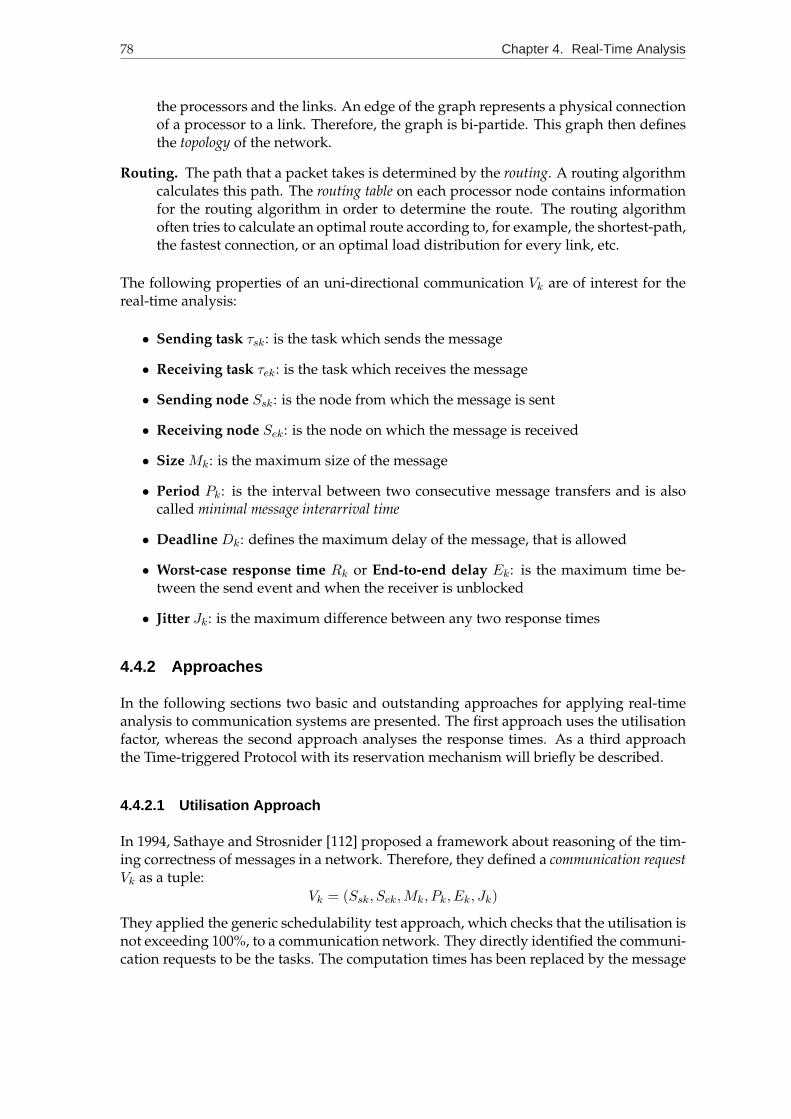
78 Chapter 4. Real-Time Analysis
the processors and the links. An edge of the graph represents a physical connectionof a processor to a link. Therefore, the graph is bi-partide. This graph then definesthe topology of the network.
Routing. The path that a packet takes is determined by the routing. A routing algorithmcalculates this path. The routing table on each processor node contains informationfor the routing algorithm in order to determine the route. The routing algorithmoften tries to calculate an optimal route according to, for example, the shortest-path,the fastest connection, or an optimal load distribution for every link, etc.
The following properties of an uni-directional communication Vk are of interest for thereal-time analysis:
• Sending task τsk: is the task which sends the message
• Receiving task τek: is the task which receives the message
• Sending node Ssk: is the node from which the message is sent
• Receiving node Sek: is the node on which the message is received
• Size Mk: is the maximum size of the message
• Period Pk: is the interval between two consecutive message transfers and is alsocalled minimal message interarrival time
• Deadline Dk: defines the maximum delay of the message, that is allowed
• Worst-case response time Rk or End-to-end delay Ek: is the maximum time be-tween the send event and when the receiver is unblocked
• Jitter Jk: is the maximum difference between any two response times
4.4.2 Approaches
In the following sections two basic and outstanding approaches for applying real-timeanalysis to communication systems are presented. The first approach uses the utilisationfactor, whereas the second approach analyses the response times. As a third approachthe Time-triggered Protocol with its reservation mechanism will briefly be described.
4.4.2.1 Utilisation Approach
In 1994, Sathaye and Strosnider [112] proposed a framework about reasoning of the tim-ing correctness of messages in a network. Therefore, they defined a communication requestVk as a tuple:
Vk = (Ssk, Sek,Mk, Pk, Ek, Jk)
They applied the generic schedulability test approach, which checks that the utilisation isnot exceeding 100%, to a communication network. They directly identified the communi-cation requests to be the tasks. The computation times has been replaced by the message

4.4. Real-Time Analysis for Communication 79
size. With this assumptions they defined, that a set of network requests is transmission-schedulable (t-schedulability), if and only if the maximum saturation of the networkSmaxis not greater than one:
Smax ≤ 1 ⇒ t-schedulability.
The maximum saturation is defined as the maximum over all saturations Si, which eachcommunication request produces:
Smax = max{Si | 1 ≤ i ≤ n}.
The saturation of a communication request is thereby defined as the minimum of allcumulative workloads Wi(t) during the interval (0, Di] normalised by time:
Si = min0<t≤Di
Wi(t)t
The workload is defined as
Wi(t) =i∑
j=1
(Cj +Ovhj)
⌈t
Tj
⌉+Ovhsysi(t) +Bi , where
Cj is the time for which the network is occupied due to the message size.Ovhj is the time for which the network is occupied due to the transmission of extra
headers, trailers, or acknowledgements. Assuming that messages have tobe split into several packets and an extra acknowledgement message in onepacket has to be transmitted before a new message can be sent, the packetoverhead Ovhj is defined as follows:
Ovhj = (Ch + Ct + Cack)⌈
CjPmax − (Ch + Ct)
⌉where
Cx is the time spent for transmitting the message, header, trailer or ac-knowledgement, respectively and
Pmax is the maximum size for a packet on the link.
Ovhsysi(t) captures communication request independent system overhead, like mediaaccess delays and overhead because of unsynchronised clocks (If the desti-nation station’s clock is ahead, then the message must be delivered with ashortened deadline):
Ovhsysi = OMAC +Oclock
Bi is the time the communication request Vi is delayed, because of the actualtransmission of a (possibly) lower priority packet due to non-preemption ofpackets on the network (priority inversion problem).
Tj is the period of consecutive message transmissions.
Sathaye and Strosnider define Smax as the “degree of schedulable saturation” metric.It can be observed that Smax is monotonically non-decreasing, if either the number ofconnections increase or each Ci or Ovhsysi or Bi increases. For this reason 1 − Smax canbe considered to be the amount of high-priority work that can be added to the system perunit time without missing a deadline.

80 Chapter 4. Real-Time Analysis
For a network consisting only of a single link, the above presented “schedulable satu-ration” metric can directly be applied. But additionally, Sathaye and Strosnider appliedthis uniform schedulability framework to three different network types by modifyingthe above described parameters. These networks are a dual link network, a token ringnetwork and a multi hop network.
Node 1 Node 2 Node n
Slot
Generator A
Slot
Generator B
...
Fig. 4.2: The DQDB network topology.
4.4.2.1.1 IEEE 802.6 DQDB The IEEE 802.6 DQDB is a dual link network, where allstations are arranged in a line with two slot generators at the ends and the links are work-ing in opposite directions (see Figure 4.2). No trailers or acknowledgments are required.But for transmitting a message a slot has to be reserved by requiring a free slot from theappropriate slot generator. A request has to be sent to the slot generator and the slot hasto arrive at the station before the message can be sent. This results into a delay of 2di, ifdi is the time for transmitting a slot between station i and the appropriate slot generator.Preemption is originally not defined in the standard, but can be achieved, because eachstation reads from the incoming link and sends the data forward on the outgoing link.Thereby, the station is able to replace the incoming packet by a new one. Thus, Ovhj ,Ovhsysi and Bi can be defined as follows:
Ovhj = Ch
⌈Cj
Pmax − Ch
⌉
Ovhsysi = 2diBi = 0
4.4.2.1.2 IEEE 802.5 FDDI The IEEE 802.5 FDDI is a Token Ring (see Figure 4.3) wherefor each station k a certain bandwidth Hk is allocated. The bandwidth is normally calcu-lated as
Hk =UkUnet
(TTRT −WT ),
where Uk is the network utilisation of station k and Unet =∑ni=1 Ui is the network utilisa-
tion. TTRT is the target token rotation time and WT is the walk time (the token rotationtime when the network is idle). A trailer and acknowledgment before sending a newmessage is not required. Assuming that a message cannot be sent while not having thetoken and while a packet is actually be transmitted (no preemption), the parameters haveto be defined as follows:
Ovhkj = Ckh
⌈Ckj
P kmax − Ckh
⌉
Ovhksysi = (TTRT −Hk)⌈
t
TTRT
⌉

4.4. Real-Time Analysis for Communication 81
Node 1
Node 2
Node 3Node 4
Node 5
TTRT
H1
H2
H3H
4
H5
Fig. 4.3: The FDDI token ring topology.
Bki = P kmax
Due to the fact, that each station can have a different Hk a new index k for the station isintroduced. Therefore, the maximum saturation Smax must be calculated over the maxi-mum saturations Skmax of all stations, which are calculated over the saturations Ski of eachmessage transmitted from this station.
...
Bus
Peer-To-Peer Link
Network Node
Ring
Fig. 4.4: An example for a multi-hop network.
4.4.2.1.3 Multi Hop Network In a multi hop network messages have to be routedthrough several stations from the source to the destination (see Figure 4.4). Each link thatthe message has to follow is named hop. The sequence of links (or stations) from thesource to the destination is named path. The transmission schedulability approach mustbe adapted by assuring that for the paths of all messages the saturation of each hop of
82 Chapter 4. Real-Time Analysis
the path P is not grater than one:
∀j ∈ P ∀i = 1, 2, . . . , nj min0<t≤Di,j
Wi,j(t)t
≤ 1,
where j refers to a link on the path and nj is the number of connections on that link.There exists only a small problem: When messages are scheduled on multiple links inseries, they may arrive at the next link before their deadline on the current link. If themessages are scheduled upon their arrival, they lose their periodic characteristics. Thisundesirable effect can be prevented, if messages arriving in a given period become eli-gible for transmission only at the beginning of the next period. This is known as doublebuffering or stop-and-go queuing [53]. This is often implemented by having an in-queueand an out-queue. Messages arriving at a station are inserted into the in-queue. Mes-sages that have to be transmitted are taken from the out-queue. Every time a period isover, the appropriate messages in the in-queue are transfered into the out-queue. Thisprocedure is known as promotion. The time between two promotions of message i on linkj of the path at station k is Ei,j + Ti,jdφpropj/T ki,je. The promotion at each station on thepath increases the end-to-end delay for the message. The end-to-end delay Ei for thecomplete message transfer on the path is not only the sum of all promotion delays oneach station, but must be calculated as:
Ei = hkEki,j +
hk∑
j=1
T ki,j
⌈φpropjT ki,j
⌉,
where hk is the number of hops on the path and φpropj is the propagation delay on link j.Thus, it should be additionally checked, whether
Ei ≤ Di.
4.4.2.2 Response Time Approach
In 1995, Tindell, Burns, and Wellings [140] considered m messages, which have to beseparated into Cm packets of constant size in each period. They tried to bound the timebetween the arrival of the sender task and the time at which the destination task is un-blocked. This time is said to be the worst-case response time Rm. They separated this timeinto different timing intervals:
Rm = Jm +Qm + ρtrans + φprop + τnotif ,
where
Jm is the generation delay, which is equal to the WCET of the sending task.Qm is the queuing delay, which is caused by previous transmission of former packets.
ρtrans is the transmission delay for one packet.φprop is the electrical propagation delay on the physical line1.τnotif is the notification delay until the receiving task really is consuming the message.
1 The electrical propagation delay may be small for a local area network, or may be very large if, say, asatellite link is part of the network.

4.4. Real-Time Analysis for Communication 83
The transmission, propagation and notification delay are assumed to be constant for eachmessage and are worst-case estimations depending on the operating system and the com-munication link and protocol.
Because the queuing delay can change in every period, Tindel, Burns, and Wellings de-fined the queuing delay Qm,q,k and therefore also the worst-case response time Rm,k ofthe k-th packet of message m as the maximum over all q-th multiples of the period Tm:
Rm,k = maxq∈IN0
(Jm + wm,q,k − qTm + ρtrans + φprop + τnotif )
Hereby, wm,q,k is the width of the level i busy period [80]. The busy period is defined as
wm,q,k = qCmρ+ (k − 1)ρ+Bm +
∑
∀h∈hp(m)∩ out(p)Ih
ρ+
⌈wm,q,kTtoken
⌉(Ttoken −Hp)
In this equation ρ is the worst-case transmission time for one packet and Bm is the delaycaused by priority inversion2 and Ih is the interference (i.e. total preemption) by mes-sages with higher priority than m (hp(m)) and sent from the same processor p (out(p)).The interference is thereby defined as
Ih =⌈wm,q + Jh
Th
⌉Ch with wm,q = wm,q,Cm
Obviously, the worst-case response time of the message is then equal to the worst-caseresponse time of the last packet of the message: Rm = Rm,Cm .
Tindel, Burns, and Wellings state that the calculation of the busy period wm,q,k can bedone by the following and simple recurrent formula:
w0m,q,k = 0
wn+1m,q,k = wm,q,k(wnm,q,k)
This formula should converge, if the utilisation is not greater than 100%:
wm,q,k = limn→∞w
nm,q,k
The above given formulas can be applied not only to token protocols, but also to prioritybusses (see Figure 4.5), like for example CAN3. For priority busses set Ttoken = Hp, sothat there is no delay caused by not having a token.
Node 1 Node 2 Node 3 Node n...
Fig. 4.5: The topology of a communication bus, like CAN. A message that is sent by onestation can be received simultaneously by all stations.
For the schedulability test it must be checked, if for all messages the worst-case responsetime is lower or equal than the maximum end-to-end delay:
∀i = 1, 2, . . . , n : Ri ≤ Di
2 The formula can be simplified if assumed that Bm = ρ.3 Controller Area Network, see [67]

84 Chapter 4. Real-Time Analysis
4.4.2.3 Time-Triggered Approach
One of the main problems that causes delays for the communication is the media access.When a packet is already transfered via the link, another packet cannot be transmittedsimultaneously. However, if this is still done, the transmission of both packets will becorrupted. For this reason, a variety of media access protocols has been developed. Apossible categorisation can be the one that is presented in Table 4.3.
Time-multiplexed Frequency-
Isochronous Asynchronous multiplexed
Controlled Accidental
Centralised/Master De-centralised/Ring CSMA CD Repetition
Single Multiple Logical Physical Priority
ATM USB VME Token bus FDDI CAN Ethernet ALOA WirelessTTP Bitbus Profibus Interbus VAN Wireless
DQDB J1850
Tab. 4.3: Possible categorisation of media access protocols and examples for their imple-mentation.
For the real-time communication mainly three media access protocols are used: isochronoustime-multiplexed protocols, token-based protocols, and priority-based protocols. The last twoones have been briefly described in the previous sections. The time-multiplexed TDMA(Time Devision Multiple Access) protocols grant each communication request or station oneor more time slots, when they are allowed to send messages. For this reason, the completeavailable time is divided into intervals (time slots). Often they are of equal size. Theassignment of time slots to messages will be done during a reservation phase.
Often the slot assignment is done statically before the run-time of the system. Thus, thetimes when communication can occur is pre-defined. This can be extended to the com-plete execution model: Also the processes are scheduled by such a fixed assignment. Theschedule is fixed and pre-defined. The execution order and the activation times for eachtask must be calculated in advance and will not change during execution. Thus, the sys-tem behaves totally deterministic and always in the same way. A famous representativefor this technique is the Time-triggered Protocol (TTP), which had been investigated in de-tail and implemented at the university of Vienna by Prof. Kopetz et al. [72]. Becauseevery action of the system is pre-defined and happens during a certain time interval,these systems are sayed to be time-driven systems. On the contrary, systems that re-act onevents are known as event-driven systems.
The MARS4 operating system [36, 73, 74] implements the TTP approach. The commu-MARSnication as well as the process scheduling are time-triggered. Thus, priorities are not re-quired. The complete time slot assignment is calculated offline during the design-phaseof the system. For the communication is assumed that all stations are attached to one bus(Ethernet or CAN). The communication in MARS is based on state messages. State mes-sages represent a kind of shared and distributed variable. Its value can be overwritten
4 MAintainable Real-time System

4.5. Resource Constraints 85
from a remote site during its pre-defined time slot. But only the actual state, which rep-resents the last write, can be read. The update of the states happens periodically. MARSdoes not offer synchronisation primitives like semaphores or a rendesvouz principle. InMARS synchronisation as well as precedence constraints must be considered during thetime slot assignment.
One of the biggest drawbacks of this approach is the request for a global clock synchroni-sation: Each station must identify the same time slot at the same time. Additionally, thosesystems are failure-prone during overload situations. Slightly shifts or moves, when spe-cific event handlings are required, are not possible. In this sense token-based systems aremore robust.
Often the periodical and static appearance of message transfers is not found in the reality.Here, often only a certain bandwidth is required, which must be mapped onto the TDMAscheme. Cruz and Turner developed a so-called leaky bucket model [77], which is used,for instance, in the ATM (Asynchronous Transfer Mode) protocol [111] in order to weakenthe synchronous TDMA scheme to an asynchronous bandwidth allocation scheme.
4.5 Resource Constraints
All the previously described scheduling algorithms assume that the tasks are indepen-dent from each other. But in most cases this is wrong. Often, tasks claim for exclusiveaccess to resources. Semaphores [21, 38, 98] or monitors [137] are used to protect such acritical section of the tasks, when it accesses the shared resource in exclusive mode. Forthis reason a task must be blocked, if the required resource is already used by anothertask. But this leads to delays of the task, which extend the finishing time. If it is known inadvance, which task claims for which resource, then the blocking times Bi for each taskcan be computed. But there exists another problem that is more severe:
The Priority Inversion Phenomenon: Assume that task τ1 has higher priority than task τ2.Despite this fact τ1 may be blocked by task τ2. If there exists a task τ3 with intermediate priority,then τ3 preempts τ2 while holding the resource, that is also claimed by τ1. The result is that task τ3
runs before τ1! Moreover, the blocking time of τ1 is unbounded if more intermediate tasks arrive.
For RM or EDF and related algorithms this means that the execution order of the taskscan be completely corrupted. The fact that a lower priority task blocks a higher prioritytask, because of requiring the same resource, is the semantic of mutual exclusion. But theproblem of the priority inversion and the unbounded delay can be solved.
Priority Inheritance Protocol. In 1990, Sha, Rajkumar, and Lehoczky [115] proposed thePriority Inheritance Protocol (PIP). The basic idea of this protocol is, when a task τi blocksone or more higher priority tasks, it temporarily inherits the highest priority of theblocked tasks. This prevents medium priority tasks from preempting τi and, therefore,they will not prolong the blocking period.
Theorem 4.1 (Sha, Rajkumar, and Lehoczky): Under the Priority Inheritance Protocol, atask τi can be blocked for at most the duration of min(n,m) critical sections, where n isthe number of lower-priority tasks that could block τi and m is the number of distinctsemaphores that can be used to block τi.

86 Chapter 4. Real-Time Analysis
Out of this theorem the schedulability test for rate monotonic scheduling [remember∑ni=1(Ci/Ti) ≤ n(21/n − 1)] can be extended to
Theorem 4.2: A set of n periodic tasks using the Priority Inheritance Protocol can bescheduled by the Rate-Monotonic algorithm if
∀j, 1 ≤ j ≤ n,j∑
k=1
CkTk
+BiTi≤ i(21/i − 1).
Here, the tasks are ordered by their priority: j > i⇔ Pj < Pi. Observe, that the equationnow must be solved for all tasks. The equation can be interpreted as follows. In order toguarantee a task τi, we have to consider the effect of preemptions from all higher-prioritytasks (
∑i−1k=1Ck/Tk), the execution of the task itself (Ci/Ti), and the effect of blocking due
to all lower-priority tasks (Bi/Ti).
What still is to be done, is the computation of the blocking time Bi for each task τi. Wecan define the ceiling C(Sk) to be the priority of the highest-priority task that may use thesemaphore Sk. With this and the definition of the Priority Inheritance Protocol we canfollow:
Lemma 4.3: In the absence of nested critical sections, a critical section of τj guarded bySk can block τi only if Pj < Pi ≤ C(Sk).
The idea for the proof is the following: If Pi ≤ Pj ⇒ τi cannot preempt τj ⇒ τi cannot beblocked by τj directly.
The blocking time Bi of a task τi can then be defined as the minimum of two differentsums of durations of longest critical sections:
Bi = min(Bli, B
si ),
where
Bli =
n∑
j=i+1
maxk
[Dj,k : C(Sk) ≥ Pi]
is the sum of durations Dj,k of the longest critical sections for any task τj with prioritylower than Pi that can block τi, and
Bsi =
m∑
k=1
maxj>i
[Dj,k : C(Sk) ≥ Pi]
is the sum of durations Dj,k of the longest critical sections for any semaphore Sk that canblock τi.
An algorithm for the computation of this blocking times is presented in [25, p. 197] andhas a complexity of O(mn2). The upper bounds for the Bl
i and Bsi are not very tight,
because two or more critical sections guarded by the same semaphore may be summed.But, if two critical sections of different tasks are guarded by the same semaphore, thenthey cannot be both blocking simultaneously. An algorithm based on exhaustive search,where all possible combinations of blocking critical sections are considered, was pre-sented by Rajkumar [103], but it has an exponential complexity.

4.5. Resource Constraints 87
The Priority Inheritance Protocol is a good solution for the problem of unbounded de-lays due to exclusive resource access. But it has two drawbacks: It does not prevent theformation of chained blocking and –as a reason of this– it does not prevent the formationof a deadlock.
Priority Ceiling Protocol. The Priority Ceiling Protocol (PCP) was also proposed by Sha,Rajkumar, and Lehoczky [115] in 1990 as an improvement of the PIP. It solves additionallythe drawback of chained blocking and prevents deadlocks. The idea of the PCP is that itextends PIP by a special granting rule for locking a free semaphore. The rule says: A taskis not allowed to enter a critical section, if there exists other locked semaphores whichcan block the task.
This is achieved by assigning to each semaphore Sk a priority ceiling C(Sk) equal to thepriority of the highest-priority task that can lock the semaphore. A task τi is allowedto enter a critical section only if its priority is greater than the ceiling of all semaphorescurrently locked by other tasks than τi. If the entering of the critical section is denied,then the task τi is said to be blocked on semaphore S∗ by the task τj that holds thatsemaphore S∗. (Note: S∗ is the semaphore with the highest ceiling of all currently lockedsemaphores by tasks other than τi.) When the task τi is blocked by task τj , task τj inheritsthe priority of task τi. In general, a task inherits the highest priority of all tasks it blocks.When a task exits a critical section, then its priority is updated as follows: If no othertasks are blocked by the task τj , it is set to its nominal priority Pj ; otherwise, it is set tothe highest priority of the tasks blocked by τj . The priority inheritance is transitive; thatis, if a task τ3 blocks a task τ2, and τ2 blocks task τ1, then τ3 inherits its priority from τ1
via τ2.
A theorem, which was given by Sha, Rajkumar, and Lehoczky, says that under the Prior-ity Ceiling Protocol, a task τi can be blocked for at most the duration of one critical section.Additionally, it follows that a critical section Zj,k (belonging to task τj and guarded bysemaphore Sk) can block a task τi only if Pj < Pi and C(Sk) ≥ Pi. From this observationwe can follow, that the maximum blocking time of a task can be computed as follows:
Bi = maxj,k{Di,j | Pj < Pi, C(Sk) ≥ Pi}.
Remark, that the calculation of the blocking times under PCP is much easier than underthe PIP. But in order to implement the PCP and to calculate the ceilings of the semaphores,all critical sections, which can be entered by any task, must be known in advance. Be-cause this is impossible for a general implementation of an operating system, nearly alloperating systems do not implement PCP.
But in TEReCS the requirement specification contains also the information about criticalsections, because the system calls on the semaphores have to be modelled in order toconfigure DREAMS correctly and to insure a more detailed timing analysis. Thus, thecritical sections are known in advance and the PCP can be implemented in DREAMS andconfigured by TEReCS.
Another quite interesting resource management protocol is the Stack Resource Policy(SRP), which will not be described here. The interested reader may be referred to theliterature (for example [25, p. 208]).

88 Chapter 4. Real-Time Analysis
Implementation ConsiderationsAll of these resource management protocols are implemented by different signal() andwait() methods. Also, the PCP does not require a waiting queue per semaphore as itwould be required in the normal case. The reason is that the task can be kept in the readyqueue since the other tasks will have higher priority. But the semaphore requires an extrafield for storing the ceiling and the process control block (PCB) requires an extra field forstoring the task’s active priority. It would be also convenient to have a field in the PCBfor the semaphore on which the task is blocked. Generally, the operating system shouldmaintain for the PCP a list of all currently locked semaphores ordered by their ceilings.
You see that the different protocols require different implementations of the operatingsystem internal data structures and functions, which are not directly related to the syn-chronisation primitives signal() and wait() . Thus, it is highly recommended to havea configuration management that takes care for a valid and working implementation ofthe operating system.
4.6 Contribution of the Chapter
This chapter gave a brief survey about the real-time problems and their solutions in thecase of scheduling, communication, and resource access.
All the different implementations of scheduling algorithms, communication protocols,resource management protocols, and their schedulability tests allow a brought varietyof combinations and selections. It should be the task of a configuration management toselect the appropriate methods and data structures in order to maintain the complex-ity of their combinations. All the different requirements of the applications and all thepossible implementations inside the operating and communication system should be de-scribed within a concept that allows to derive a description for the configurator’s domainknowledge bases. This task is the motivation for the next chapter.
CHAPTER 5
From Taxonomy Towards Configuration Space
In this chapter the attempt is made to identify characteristics of real-time systems bywhich they can be categorised. These characteristics are ordered within a taxonomy. Thistaxonomy is important for the completeness of this thesis. It can give hints, where con-figuration of a run-time platform for a real-time system makes sense, i.e. where con-figuration should be done in order to improve the system’s efficiency. The dimensionsor domains that span the taxonomy can define the items of a run-time platform, whichare configurable. It should be clearly mentioned that the taxonomy, which is developedhere, is especially designed for this purpose. That means that there may exist other tax-onomies, which are designed for other reasons.
The Table 5.1 on the following page is an attempt to identify properties by which a dis-tributed real-time system can be classified. The different properties describe differentoperating system implementations, whereas for one class of properties all operating sys-tem implementations are equal. Formally speaking, the taxonomy defines equivalentclasses of real-time systems, where for each class the operating system is fixed and doesnot change.
Obviously, the taxonomy can describe systems that are impossible to implement and,therefore, an operating system that ensures a temporal execution does not exist. Forexample, the precedence constraints of the tasks define a deadlock or the cumulativeworkload of a processor is exceeded. Thus, a system including the final operating systemshould be analysed for its correct execution. This analysis phase should be done after theconfiguration phase, because configuration decisions have impact on the execution, i.e.the operating system overhead can differ.
In the next few sections the impact of the taxonomy items on the operating system con-figuration will be described in more detail.

90 Chapter 5. From Taxonomy Towards Configuration Space
5.1 Taxonomy for Real-Time Systems
In order to identify configuration items for an operating and communication system theproperties and characteristics and even implementation possibilites of distributed real-time applications should be investigated in general. In the following sections some di-
Global System Model and System Behaviour
• time driven vs. event driven (polling vs. interrupts)•mono-programming vs. multi-programming• static vs. dynamic (creation of new tasks)• deterministic vs. non-deterministic
(worst-case execution time vs. average execution time,connection- vs. packet-oriented communication)• distributed vs. local vs. centralised
Task Characteristics
• periodic vs. aperiodic vs. sporadic• preemption vs. no-preemption• constraint types:− resource constraints
(critical sections)− precedence constraints
(communication, priority)− timing constraints (deadlines)− criticalness:
? hard, firm, soft
Communication Characteristics
• periodic vs. aperiodic vs. sporadic• channel- vs. packet-oriented• preemption vs. no-preemption• constraint types:− resource constraints (bandwidth,
time slots)− precedence constraints (priority)− timing constraints (deadlines
end-to-end delays)− criticalness:? hard, firm, soft
• peer-to-peer vs. broadcast vs. multi-cast (1 : 1, 1 : m, n : 1, n : m)• buffered vs. unbuffered (size)•maximum message size• no loss of message order• guaranteed transmission (acknowledgements)• error detection• error correction
Machine and Hardware Properties
• single-processor vs. multi-processor• homogeneous vs. heterogeneous processors (endianess, speed, memory size)• shared vs. distributed memory• interconnection network:− topology (peer-to-peer, bus, ring, etc.)− unidirectional vs. bidirectional links− neighboured communication vs. multi-hops− homogeneous vs. heterogeneous links−media access protocol per link−maximum packet size per link− delay of packet per link− transfer time of packet per link
Tab. 5.1: Dimensions of a taxonomy for real-time systems.

5.1. Taxonomy for Real-Time Systems 91
mensions will be presented, for which the implementation differs in order to meet specialproperties of the application. These application properties can form the dimensions of ataxonomy, by which the implementations can be classified. That means, if the value of ataxonomy’s dimension differs for different applications, then the implementations of theoperating and communication system will be different, too. Therefore, on the one handthe implementations will belong to different classes of applications. On the other hand,if the values of all dimensions are the same for different applications, then the imple-mentation of the operating and communication system will also be the same. Thus, theapplications belong to the same taxonomy class.
The dimensions of the taxonomy can be categorised into four different major domains.These domains group dimensions concerning properties of the system model and thesystem’s behaviour, task characteristics, communication characteristics, and properties ofthe distributed machine (hardware) on which the system should run. These domains hadbeen identified, because they tackle different aspects of the application’s implementation.Moreover, we will see later that these taxonomy domains will result into different partsof a requirements specification.
5.1.1 System Model and System Behaviour
Time driven or event driven: Time driven means that inputs are regarded at fixed ab-solute times (i.e. the system is polling). Event driven considers events to be taken attheir arrival. Thus, the system has to handle interrupts. To have interrupts or not makesa big difference for the operating system, because interrupts require a special treatmentlike saving the context and restoring it. In contrast, time driven systems require a globalclock in order to synchronise.
Mono-programming or multi-programming: This property defines whether the pro-grammer specifies a single task or has multiple tasks running simultaneously. If thisproperty is regarded per node (processor) of the system, then obviously, the question forrequiring a task switching mechanism (scheduler) per node can be answered.
If the system behaviour can be regarded to be static (the task set and its properties donot change during execution), then the scheduling algorithm can be simpler and the taskset’s feasibility test can be done offline. For example, the simplest scheduling schemeapplied to a static task set is a fixed activation order. On the other hand, if tasks can arrivedynamically, then the operating system must integrate an acceptance test and possibly,the scheduling algorithm requires preemption, which requires again saving the contextand its restoration.
If the system is deterministic, then it is said to be predictable. In this case the conven-tional management strategies (like RM, DM, LDF, EDD, EDF, etc.) for the task set canbe applied. But, if some of the system’s tasks are not deterministic, then assumptions orprobabilities about their properties are made. In this case the so-called server algorithmsfor aperiodic task scheduling should be considered.
A centralised distributed system requires more powerful hardware for the server and,therefore, other system services than a homogeneously distributed system. A client/serverimplementation has other requirements than distributed agents. Especially, the bottle-neck of a centralised server with applied high performance services or the load balancing

92 Chapter 5. From Taxonomy Towards Configuration Space
service for a highly dynamic system should be considered.
5.1.2 Task Characteristics
A task set can be regarded periodic, aperiodic, or additionally contains sporadic tasks.This has direct impact on the schedules for a timeliness execution. Obviously, for thisreason the scheduling algorithms, which had been introduced in Chapter 461, had beendeveloped.
Additionally, all the task properties themselves allow or forbid a specific scheduling al-gorithm. These are especially properties classifying the algorithms into categories (seeTable 4.171 and Table 4.274). If a task allows preemption, has precedence, resource, ortiming constraints, then these properties demand for a special treatment by the sched-uler. Moreover, synchronisation by signal() and wait() or semaphores has to beconsidered. Thus, PIP, PCP, or SRP come into the picture.
When tasks run quasi-parallel on a processor, because they can be preempted, then mu-tual access to shared resources is requested. The internal state of a resource must notbe changed by more than one task simultaneously. Otherwise, data integrity or correctbehaviour is not guaranteed. Thus, tasks use operating system primitives for synchro-nisation and protection, like semaphores, monitors, or simple signal() and wait()primitives. The usage of these primitives requests for a special functionality of the op-erating system. Additionally, these synchronisation primitives have great impact on thescheduling, because tasks might be delayed (blocked). In order to assure a special be-haviour the synchronisation protocols PIP, PCP or SRP had been designed.
Many scheduling algorithms and their analysis assume that the given tasks are indepen-dent from each other. But when a single application is split into several tasks in order toexploit inherently possible parallelism, then these tasks work normally on data, which isforwarded and manipulated from task to task in a pipelined manner. Examples may bestreaming applications, where filter, conversion, and Fourier transformation algorithmsare sequentially ordered. Other examples may be control algorithms, where subsequentcontrollers read input values that had been produced by other controllers. Controllerscan also be arranged hierarchically, where top-level controllers (e.g. the body controlof a car) have influence on low-level controllers (e.g. active suspension) by generatingappropriate control values. These in/out dependencies between tasks request for com-munication. Thus, communication demands should very carefully be investigated andcan have great impact on the running task set.
If these tasks are local to a processor and, for example, use shared memory communica-tion, then the communication problem can be transformed into a resource and synchroni-sation problem. But when the task set is distributed over several processor nodes, whichare interconnected by communication links, then the calculation of the delays becomemore complex. This is because of mutual influences of tasks that are not directly commu-nicating but acquiring shared resource access of the links. The situation becomes moresevere, when for the message transfer several links have to be traversed, because there isno direct connection between the sending and receiving processor. For this reason, thecommunication in a distributed real-time system should be investigated in detail.

5.1. Taxonomy for Real-Time Systems 93
5.1.3 Communication Characteristics
As seen from the analysis of communication systems the properties of a task set canbe transferred to a set of messages. Messages can be periodic, aperiodic, or sporadic.This mainly has impact on the reservation scheme for the bandwidth (which is equal tothe processor allocation). Periodic messages often have to be established by channels.Thereby, bandwidth or time slots of the links are reserved. This allocation scheme isnamed channel-oriented communication. This method is also recommended, if the maxi-mum delay of a message transfer should be predictable. So, real-time messages shouldbe handled always channel-oriented. On the other hand, packet-oriented communicationexists. This method is to be preferred, if no reservation has to be done or the messagetransfer time cannot have unlimited delays. Unbounded delays occur, when the messagetraffic in the network is not predictable. Often, packet-oriented communication worksonly with a best-effort strategy for delivering messages.
Another very interesting property of a message transfer is, that a message can be pre-empted during the transfer. Here, preemption is relatively more severe, because the mes-sage again has to be completely transferred after a preemption occurred. Thus, preemp-tion destroys a message transfer. For this reason, protocols often do not allow preemp-tion.
Precedence constraints also exists for messages. Often for communication, the sendingand receiving of messages have to preserve the message order. This means, if a mes-sage a was sent before a message b, then the message a should arrive before message b.This can either be assured by the rule, that messages cannot overtake other messages,or the receiver protocol stack delivers unordered received messages only ordered to theapplication, by considering message numbers and buffering of orderless messages.
Resource constraints of messages have to be considered implicitly, if the channel-orientedcommunication is used. Here, the route and, therefore, the links that the message has totake for each hop are fixed. Routing has a major impact on the resource constraints ofa message. The routing is steered by the origin and destination of the message. If thesender is fixed, we distinguish peer-to-peer (1 : 1), multi-cast (1 : m, m < n), or broadcast(1 : n) messages (where n is the total number of all destinations). If we do not have theclassical peer-to-peer (P2P) case, then it depends on the topology, if messages have to beduplicated and have to be sent simultaneously on multiple links. Often ignored is thecase, when several sources send messages to a single destination (m : 1), like clients sendmessages to a server. The receiver must have the ability to await messages from differentsources.
If messages have to take several links in order to reach their destination, then the mes-sages sometimes have to be stored into buffers on intermediate nodes, before they areforwarded (see “stop-and-go queueing” on page 82). For embedded systems with hardresource constraints, the maximum required buffer size must be known in order to savememory and to guarantee no message loss.
Another problem arises and has to be investigated, when the maximum packet size on alink is smaller than the message size. Then, a message has to be split into several packetson the sender side and the packets have to be assembled to the original message on thereceiver side. Here, problems like ordering, buffer size, and preemption have again to beconsidered. Even, if a packet on a link cannot be preempted, the complete message can

94 Chapter 5. From Taxonomy Towards Configuration Space
be delayed, because the sending of a packet can be delayed by packets of other messagesdue to media access problems. These media access problems occur, because during therequired setup-delay for a new packet, another node can acquire the media. If packetshave priorities, then this problem can be much more worse and can result into priorityinversion.
Sometimes the transmission of a message cannot be guaranteed by the physical architec-ture of the link. A message can be completely lost or is partly corrupted during the trans-fer. But the application demands for correct transmissions and no message loss. Then,the communication protocol has to assure error detection and correction. This sometimesrequires the re-transmission of a previously corrupted or lost packet. Thus, positive ornegative acknowledgements are sent in the opposite direction than the communicationitself. For this reason backwards channels have to be established. These channels acquireadditionally bandwidth and have to be handled not only by the protocol, but also by theanalysis.
5.1.4 Machine and Hardware Properties
Characteristics of the machine and hardware have also impact on the configuration. Theprocessor architecture itself selects or forbids services, because the services are using aconcrete assembler dialect or other hardware specific features. Moreover, processor ar-chitectures might use different orderings for storing their high and low bytes of words(big or little endian storage). If packets are transmitted between tasks running on suchdifferent processors, the byte ordering of the packet for each number compound, whichis greater than a byte, must be changed at the sender’s or receiver’s side. Thus, one pro-tocol stack has to deal with this conversion and has to be enriched by an appropriatefunctionality.
The processor architecture is also of great interest for the analysis . The same service canhave different worst case execution times due to different processor speeds, caching, orpipelining, etc.
Not only the processor architecture, but also the concrete devices, which have to be man-aged by the operating system, require specialised device drivers. This problem is alreadywell known for general purpose operating systems like WindowsTM or Linux. But it be-comes more difficult for embedded and real-time operating systems. Even for the samedevice the driver implementation should differ due to different use cases. The commu-nication devices and protocol stacks are considered especially in this thesis, because ofthe distributed aspect of the targeted application scenarios. It is the primary goal of theconfiguration aspect to support the application with the optimally adapted services withthe best efficiency and to remove unnecessary features from the operating and commu-nication system. Additionally, it should be tolerable to specify a lot of services, devices,and/or connected links per processor. The final application requirements should deter-mine, which services, devices, and links are really used and which are not. This implicitlydetermines whether a driver is required or is not required.
A very important property of the hardware, which has impact on the link usage, is thetopology of the interconnected processors and links (media). Required communicationis routed through the network by determining a path that the message has to use. Sucha path describes the resources, which has to handle the message. These are devices for

5.2. Configuration Items 95
the sending and receiving, as well as media for the transport. Additionally, processorsare specified for the sender and receiver and for intermediate nodes (hops), at which themessage has to be forwarded. The topology greatly determines whether forwarding isrequired or not. Forwarding of messages often requires dynamic routing and bufferingof the messages. If forwarding can be omitted, then the system overhead due to commu-nication can dramatically be reduced.
If forwarding is required, then another problem arises. Each communication media de-fines its own protocol stack, which is used for the sender and receiver side. If on thepath different in- and out-links are used, then on such intermediate nodes two differ-ent protocol stacks have to be bridged. Bridging means protocol transformation, whichadditionally leads to system overhead and have to be coped by the involved protocolstacks.
Each type of hardware link and protocol stack require special communication drivers.Thus, the system overhead is different. Moreover, each link architecture and its mediaaccess protocol cause different transmission times and delays for the packets. This has tobe considered by the analysis.
5.2 Configuration Items
Until now the different requirements that an application may seek for have been iden-tified. These requests form the dimensions of the previously presented taxonomy. Theprimary goal is to identify items or entities within an operating and communication sys-tem that have other implementations in different taxonomy classes. These changes fromone taxonomy class to another and the reason for these changes have to be formally de-scribed. This formal description spans the configuration space for the operating andcommunication system.
But, how do we identify different implementations for other taxonomy classes? Fortu-nately, this is easy. Researchers have already identified properties of different applica-tions, which in fact define the taxonomy, and, therefore, they “invented” different im-plementations leading to better results for the concrete case (taxonomy class). For ex-ample, there exist different implementations for scheduling algorithms, because specialtask set properties require special treatment in order to achieve the best performance.There we find the relationship between properties or requirements of the application andexchangeable items inside the operating system.
Implicitly, these relations have been mentioned while the different properties, character-istics, and requirements of the taxonomy were presented. These items have been gath-ered in Tab. 5.2 on the following page. On a very high level some areas of an operatingsystem can be identified by grouping exchangeable items together, which are influencedby the same characteristics of the taxonomy. For instance, all the scheduling algorithmsare grouped into the group of scheduler services, because they depend on the properties ofthe given task set.
Yet another example would be the protocol services that depend on the properties, whichmust be assured during the message transfer. In fact, the protocol does not only dependon the required quality of service (QoS) for the message transfer, but it also depends onthe hardware capabilities of the communication link. This is an example where more

96 Chapter 5. From Taxonomy Towards Configuration Space
than one taxonomy dimension (QoS of message transfer and hardware properties) haveimpact on the same item (protocol). Two dimensions have to be matched by the config-uration, that means by the final implementation. The solution employs protocol stacks,where on each level the protocol can be exchanged in order to achieve the desired QoS.Moreover, the application can access the protocol stack at different levels or the hardwarerequests for a special low level protocol. Additionally, the protocols rely hierarchicallyon each other. Each demand for a specific quality for the communication service requestsfor a specific protocol. Each protocol itself requests for an appropriate lower level proto-col, until a protocol is reached, which handles the communication link. This is the lowestlevel of a protocol stack, which is often named link layer (e.g. see OSI model [66]). This is a
Global Services
• interrupt management (context saving)• synchronisation (signal and wait)• scheduling•memory management• communication• repositories/databases/lists/arrays• timer management (task suspension by timer sleeps)
Task Scheduling(per processor)
• off-line schedulability vs. on-lineacceptance test• global policy (deadline, slack, remaining,
execution time, dynamic, server, etc.)•multi-level hierarchy (per level):− algorithm (EDD, LDF, EDF,
DM, RM, PS, DPE, etc.)− ordering (deadline, priority,
remaining execution time,slack time, FIFO, criticalness, etc.)
• dispatching scheme− context switch time (> 0 ?)
• real-time support yes/no• critical section yes/no− algorithm (semaphore, mutex, monitor,
etc.)
Communication Scheduling(per link)
• off-line vs. on-line− bandwidth/time slot reservation− channel establishment
•multi-level hierarchy (per level ofprotocol stack):−max. packet size− protocol:? preserving message order? error detection/acknowledging? error correction? buffering? forwarding (device usage)? reception (device usage)? splitting? duplicating? delivering? routing? conversion (bridging)
− protocol overhead−maximum delay
Hardware Interface
• resource usage− device interrupts− exclusive device access− device parameters (address, baud rate, memory usage, etc.)
Tab. 5.2: Configuration items.

5.3. Creating the Configuration Space 97
step-wise refinement of the requests, where the requests that are leading to sub-requestsof the sub-layer are transitive.
At a very high level the services of an operating and communication system that areinfluenced by a certain domain inside the taxonomy can be grouped into:
• interrupt management services• scheduling services• synchronisation services• memory management services• communication services• repository services• time management services
Each of these groups can be divided into sub-groups, which depend on a different do-main of the taxonomy’s dimension. A domain of the taxonomy is defined as a specificset of properties, characteristics, or requests. The different values or instances of this do-main directly lead to different implementations of a specific operating system function.For instance, the domain to implement the system time driven or event driven, requestsfor timers or interrupt functions (or both, if time driven and event driven is mixed). Thedomain of tasks that have critical sections requests for synchronisation mechanisms likethey are supported by semaphores, mutexes, monitors, etc.
In Table 5.2 on the preceding page, besides the high level service groups, the sub-groups,for example, for task scheduling and for the communication services, have been sketched.At the bottom of all configurable (selectable) items we find the hardware. Here, the hard-ware resources are enumerated, which can alternatively be used. The demands of thetaxonomy for special hardware domains requires specific resources to be present or not.
The resources are not only defined by the required hardware dimensions, but also by theapplication’s dimensions (demands). The application’s demand for a broadcast prefersa communication bus in contrast to a peer-to-peer network. Nevertheless, the applica-tion demands and the hardware properties define a trade-off, which has to be solved bythe configuration process. Besides the resource selection, parameters for the resourcesmust be determined. The resource itself as well as its parameters can be identified asconfiguration items that have to be assigned to concrete values.
5.3 Creating the Configuration Space
Previously, we have identified a taxonomy, which led directly to the configuration itemsin an operating and communication system. Now, we need to develop a formal represen-tation for the configuration items and their dependencies. This description should spanthe design space of all operating system classes that are formed by the taxonomy.
The alternatives of a dimension in the taxonomy identify exchangeable items in the im-plementation. Such alternatives naturally define an OR-group. For example, the dimen-sion of scheduling services contains all alternative scheduling algorithms. But only onealgorithm should be implemented. Another example is the critical section domain, whichconsists of alternative synchronisation algorithms. On the one hand, either one item of a

98 Chapter 5. From Taxonomy Towards Configuration Space
set of alternatives is required or none of the items are availed. Thus, the OR-group shouldallow no selection. On the other hand, sometimes more than one alternative should be se-lectable. An example can again be the critical section domain. Because tasks differ in theirimplementation model, the tasks can request different synchronisation algorithms. Thisimplies, that for instance, the operating system has to support semaphores and monitorsat the same time. Thus, side constraints can have impact on the domain’s value selection.
If a value in a domain is another domain, then this is a transitive request. In the previoussection we said this to be a refinement of a request. For example, a scheduler can be anon-real-time scheduler or a real-time scheduler. Both requests or items can be refined asshown in Table 5.3103 and form a domain by themselves. This directly defines a transitivedependency between two domains (OR-groups).
Often, the dependencies between values of the taxonomy domains and other domainsare manifold. For instance, the Round-Robin scheduler is a value of the scheduler do-main and, therefore, it is part of an OR-group of all scheduler services. If the preemp-tive Round-Robin scheduler will be selected, then it requires a periodic timer interruptand a queue in order to manage the FIFO list of all the ready tasks. This is a classicalAND-group of simultaneously required sub-services. Here, these sub-services are itemsof other domains. In this case these domains are time management, interrupt managementand repository. For this reason, if all AND/OR-dependencies have been found, then nota tree will be the result, but an AND/OR-DAG (Directed Acyclic Graph) will describe thedesign space of all configurable items.
driver a driver ddriver b driver c
link layer
message splitting
routing
endianess conversion
bandwidth allocation
unreliable send reliable send
TouCANAddr. 1
TouCANAddr. 2
CAN 82825Addr. 3
Serial RS232Addr. 4
FirewireAddr. 5
message parameter:sizesenderreceiverdriver address
processor(all receivers) <> constant
endianess (processor(sender)) <> endianess (processor(receiver))
driver address (message)
error correction
packet size (driver(driver addr.))< size (message)
Fig. 5.1: OR-DAG that is representing one possible real-time communication stack.
In Figure 5.1 an example for a customisable real-time communication stack is sketched.Only the sender side of the protocol stack is displayed. Each oval node of the graph

5.3. Creating the Configuration Space 99
represents a protocol layer, respectively a software service of the operating system. Therectangles at the bottom of the graph represent hardware devices, via which the messagescan physically be sent. At the top of the graph the two nodes unreliable send and reliablesend are the interface functions of the API (Application Programming Interface). Thesefunctions can be called from the application in order to send a message. Because theyserve as root nodes of the graph, they are called primitives in this thesis.
The directed edges between the nodes describe the calling dependencies within the pro-tocol hierarchy. That means, if there exists an edge from a protocol A to a protocol B (orto a device b), then protocolA requests for protocolB (or the device b) in order to achieveits function. When more edges are leaving a node, then all sons form an OR-group. Allnodes of an OR-group can alternatively be selected in order to serve for the function ofthe father-node. Therefore, the graph in Figure 5.1 on the facing page is only an OR-DAG.There does not exist any AND-relation.
The OR-group can be an exclusive OR, which means only one successor must be selected,or a normal OR, which means that at least one successor must be selected. All ORs thatare depicted in Figure 5.1 on the preceding page are exclusive ORs, except the ORs of thelink layer and its drivers.
It can be observed that the protocol services endianess conversion, routing, message splittingand error correction can be omitted from the protocol stack. In Figure 5.2 a simple examplefor a service that can possibly be omitted is depicted. Assume that service A is alwaysrequired. The service B can be ommited, because for service A the services B or C canbe alternatively be selected. The service C is always requested, either directly by A orindirectly by B. Thus, in a final configuration either all three services must be presentor only A and C. If each service produces costs, then selecting only A and C is cheaper.But side constraints can additionally request for service B. For that case, B cannot beomitted.
The protocol services in Figure 5.1 that can be omitted are only requested, if special con-straints of the messages, which are all sent via the two sending primitives, hold. Theconstraints are shown by the rectangles with one marked corner. The text inside therectangle describes briefly and informally the constraint. Therefore, we assume that mes-sages have certain parameters, like the sender and receiver node identification, and thesize of the message. The driver address, which is to be used in order to send the messagephysically, is determined by the routing protocol.
The configuration problem is to select only the minimal set of required services and de-vices of the OR-DAG in Figure 5.1. This is to be done in a way, that all messages, whichwill be sent via the two root primitives, can be delivered to their receivers. For exam-
A
B
C
Fig. 5.2: Technique in an OR-DAG for eventually omitting a service B.

100 Chapter 5. From Taxonomy Towards Configuration Space
ple, the protocol service error correction is not required, if no message will be sent via theprimitive reliable send. Or, the protocol routing is not required, if all messages that will besent, must be sent via the same device. Thus, during configuration for each message apath from the used sending primitive down to the appropriate device have to be found.Additionally, all constraints must be considered. The services and devices of all pathsmust be selected for the final configuration.
The description of the OR-DAG in Figure 5.198 is done on a very high level of abstrac-tion. For a real usable configuration space description it has to be refined and must bedescribed more formally. One possible way for such a description will be developed inSection 6.3108. Additionally, for real message transfers the receiver’s protocol stack mustbe considered similarily. Moreover, there will exist constraints between the services ofboth protocol stacks, respectively OR-DAGs. For instance, if the protocol service messagesplitting on the sender’s side is selected, then on the receiver’s side the opposite protocolcombining packets must be selected. Or none of these protocols at all must be selected onboth sides.
5.4 “Puppet Configuration”
As we have seen in the sections before, a taxonomy for distributed real-time systems candefine the requirements, properties, and characteristics, which split the implementationsof an operating and communication system into different classes. These requirements,properties, and characteristics can be interpreted as the demands of the application ofa real-time system. For this reason, these items define a requirements catalogue. Thiscatalogue is the basis for a requirements specification.
We have also seen that the domains of this taxonomy (requirements specification) natu-rally define an AND/OR-DAG by refinement. The refinement of domains leads to theidentification of configuration items (alternative services) inside the operating and com-munication system. Sometimes, they classify the operating and communication system’simplementations into instances, where a special service must be present, or is not re-quired. Often, they define alternatives. Either the alternatives of an implementation arealready known (because of research, e.g. in the area of real-time analysis) or they caneasily be identified. By definition a property of the taxonomy splits the implementationsinto (at least) two different instances. Thus, this entails that implementations handle thisspecial aspect of the taxonomy in appropriate ways.
During this refinement process some sub-domains have to be created, which result intoadditional requirements. They have only to be evaluated, if the top-level-domain is alsorequired. Hence, these sub-domains have to be evaluated during the refinement of theconfiguration. While questions are answered, additional questions arise, which also haveto be answered. This is a sort of depth-search in the AND/OR-DAG until we havereached domains with no sub-domains. In this sense, configuration means to find ap-propriate paths from each top-level domain to sub-domains, which are not again refined.Thereby, the selection of one or a set of values for a domain leads to a specific sub-domain.Only sub-domains of selected branches will be taken into consideration.
The AND/OR-DAG, which is the result of the refinement process for the demandedproperties of all applications, spans the complete design space of the operating and com-

5.4. “Puppet Configuration” 101
munication system. This design space describes by its alternatives all the different imple-mentation classes. In fact, there can be a lot of classes.
The top-level domains of the taxonomy (primitive usages defined in the requirementsspecification) serve as starting points for the search in the AND/OR-DAG of one oper-ating and communication system’s design space (see Section 6.4.3115 and Figure 6.5116).The fixing of a domain’s property to a concrete value is possible by answering the ap-propriate question of the requirements specification. Thus, by giving answers to thosequestions, the alternatives inside the AND/OR-DAG can be selected. This is similar toplaying a puppet (see Figure 5.3).
Application uses Primitives of the Design Space
Pulling the Strings of a Puppet
Puppet Configuration
Primitives
USG
Fig. 5.3: The basic idea of “Puppet Configuration”.
The puppet player pulls the strings of the puppet in order to change the spatial arrange-ment of the puppet’s skeleton. If we would take a picture of a puppet, then this pic-ture would show one specific configuration of all possible arrangements of the puppet’spieces. We can transfer this example to the taxonomy’s AND/OR-DAG. While a spe-cial property of the taxonomy is selected and instantiated with a concrete value, we di-rectly select one alternative of an OR-group. This way, we have captured a special aspect,which, for example, means the move of an arm of the puppet. But in order to touch anitem with the puppet’s hand, we have also to move the hand. This is similar to the re-quest for a sub-domain of the taxonomy to be answered. Moreover, by pulling one stringof a puppet, more than one “bone” of the puppet will be moved. This is also true forthe AND/OR-DAG and the taxonomy. Inside the DAG hierarchy the selection of onespecial property to a concrete value can have impact on more than one domain, becausethe domains are members of a transitive relation. The joints in-between the bones of thepuppet are representing this transitive relationships and some side-constraints inside theAND/OR-DAG.
The AND/OR-relationships are not sufficient to describe the design space of an oper-ating and communication system. This we have seen in the example in Figure 5.1 98.

102 Chapter 5. From Taxonomy Towards Configuration Space
Additionally, constraints have been defined. The AND- and OR-relations describe onlythe alternatives of a configuration. The constraints describe, which alternatives have tobe taken upon some parameters of primitive usages. Although, the selection of the prim-itives determines which sub-graphs have to be considered, the constraints determine theselection of the correct branches in this sub-graphs.
The constraints can be categorised into different types. The first type that we have ob-served in the protocol hierarchy has been the costs per selected service. The overall costsfor a complete path down from the primitive to the devices have to be minimised. Otherconstraints had been defined for parameters of the primitive usages. Thus, certain condi-tions defined upon properties of the messages that are sent via that primitives force theselction of specific alternatives. Besides forcing a service also the deny of the selectionof a service in an OR-group is possible. Additional types of constraints might be useful.They will be described in Section 6.3.4110.
5.5 Conclusion
The taxonomy of Table 5.190 is neither complete nor the only possible solution. It hadbeen organised to have a first starting point for the design of a configuration descriptionof a customisable operating and communication system. The domains of the taxonomyprecisely describe the questions of the requirements specification that must have impacton configuration decisions. This led to the idea of “Puppet Configuration”, which is de-scribed in Section 5.4100. Moreover, the taxonomy’s dimensions give very good abstrac-tions for the configuration decisions.
Other taxonomies contain the configuration items itself. They contain the instantiatedscheduling scheme, synchronisation algorithm, driver, or protocol. Here, these itemsare regarded implicitly on the lowest level. Hence, they are candidates for configuration.Thus, the taxonomy presented here and their configuration items are often mixed in othertaxonomies, although they have direct or indirect impact on the operating and communi-cation system. The taxonomy presented here contains only indirect properties which arecandidates for a requirements specification, whereas the direct properties are candidatesfor the description of the configuration space. The dependencies from indirect to directproperties can be regarded as the strings that have to be pulled in order to change fromone configuration to another.
Pulling the strings of a puppet can be compared to answering questions of the require-ments specification. The string is replaced by a user primitive that will be used by the ap-plication. In order to change the configuration of a puppet the strings have to be pulled.For the AND/OR-DAG this means to select appropriate user primitives. The distance withwhich the string is pulled can be compared to the parameters of the user primitive’s usageor the number of a specific user primitive call.
In this chapter we presented a motivation for the graph- and structure-based configura-tion approach in TEReCS. We argued that the refinement of requests from the require-ment specification leads naturally to sub-requests. Hereby, the sub-requests can be alter-natively be solvable or they must all be solved, like in a problem reduction graph. Thenatural representation for this in general is an AND/OR-DAG. The sub-requests formagain other dimensions of the taxonomy. Mutual influences between different dimen-

5.5. Conclusion 103
interrupts/polling ⇒ context saving for interrupts yes/no
task creation ⇒ online acceptance test =⇒ EDF, EDF∗, server
guarantee/best effort ⇒ hard/firm scheduling
multi-/mono-programming ⇒ scheduler yes/no
scheduler ⇒ Non-RT scheduler, RT scheduler
Non-RT scheduler ⇒ FIFO, RR
RT scheduler ⇒ RM, DM, EDD, LDF, EDF, EDF∗, server
periodic tasks ⇒ timers and periodic scheduling
timing constraints ⇒ synchronous activation , periodic tasks, ape-riodic tasks, mixed periodic/aperiodic, dead-line, preemption, precedence constraints
timeouts/sleeps ⇒ timers
periodic scheduling ⇒ RM, DM, EDF, EDF∗
deadline = period ⇒ RM, EDF
aperiodic tasks ⇒ EDD, LDF, EDF, EDF∗
synchronous activation ⇒ EDD, LDF
preemption ⇒ EDF, EDF∗, dynamic server
precedence constraints ⇒ LDF, EDF∗
mixed periodic/aperiodic ⇒ EDF, EDF∗, server
response time improvement for aperiodictasks
⇒ server
server ⇒ fixed priority or dynamic server
resource constraints ⇒ PIP, PCP, SRP
periodic messages ⇒ channel-oriented
channel-oriented ⇒ bandwidth allocation and management
aperiodic messages ⇒ packet-oriented, channel-oriented
message preemption ⇒ detection, acknowledgement
order preserving ⇒ sequencing, FIFO
peer-to-peer ⇒ fixed routing
multi-cast ⇒message duplication or bus
broadcast ⇒message duplication or bus
client/server model ⇒ alternative receive on multiple input channels
packet size < message size ⇒ splitting
guarantee ⇒ acknowledgement and error correction
graph mapping: communications into topol-ogy→ hopping
⇒ routing
hopping ⇒ forwarding
message buffering ⇒mailboxes
dynamic channel creation ⇒ online bandwidth management
Tab. 5.3: From taxonomy to configuration items.

104 Chapter 5. From Taxonomy Towards Configuration Space
sions of the taxonomy exist. This is the reason, why additionally constraints must beintegrated into the model. They help to solve alternative requests and to correlate thetaxonomy’s dimensions.
5.6 Contribution of the Chapter
This chapter presented a taxonomy for real-time systems that leads to a model for thedesign space description for the configurable options of a real-time operating and com-munication system. It motivates why the solution, which is used in TEReCS and that ispresented in the next chapter, uses a graph- and structure-based configuration approachbesides the integration of constraints. Additionally, the idea of the integration of ap-plication specific knowledge into the configuration process is presented as the “PuppetConfiguration” approach. This seems to be very suitable for the configuration of serviceplatforms like operating and communication systems.

CHAPTER 6
TEReCS
The real-time system’s designer now has the techniques available to engineer systemsrather than just to build them and then see if they meet their requirements
during extensive (and expensive) testing.
Alan Burns, 1993 [23]
This is the main chapter of the thesis. Herein, all of the new ideas and concepts of TEReCS(Tools for Embedded Real-Time Communication Systems) are presented. Also, the solu-tion for the problem of Section 2.212 is given.
The main objective of TEReCS is the generation of optimally adapted operating systeminstances for a parallel service platform, which serves a distributed embedded applica-tion. The communication dependencies between the distributed tasks are mainly consid-ered. Moreover, in the focus of TEReCS lies the desire to support an optimal and temporalcorrect communication inside the distributed parallel machine of the embedded controlunits.
In the first two sections of this chapter an overview about TEReCS and its concept isgiven. The model and the method for the description of the knowledge bases and the in-puts for the configuration process are presented in Section 6.3. In this model the detailedinformation about the structural properties of the configurable communication and op-erating system are hidden from the user. The configuration process, which is describedin Section 6.4, is extended by a hierarchy concept in Section 6.5. After the basic conceptshave been presented the languages for the inputs to TEReCS are defined (see Section 6.6).Additionally, it will be explained in which way TEReCS is applied to the customisable op-erating system library DREAMS. Hereafter, the knowledge transfer from the applicationto TEReCS in order to configure the operating systems and the communication system isexplained (see Section 6.7). In Section 6.8 the concept of the real-time analysis in TEReCSis presented. The chapter ends with some examples that show the mutual influence of

106 Chapter 6. TEReCS
the configuration (see Section 6.9) and analysis phase (see Section 6.10) in TEReCS.
6.1 Overview
TEReCS covers two main aspects for the development of embedded real-time systems.First, TEReCS is a software synthesis system for the generation of distributed (multi-processor) real-time operating systems (RTOS) and a real-time communication system(RCOS) from an operating system library kit. Second, it supports and ensures real-timeproperties of the system. The main goal of the system is the generation of an individualRTOS for each node of the target system. The RTOS should be optimally adapted to therequirements of the application. Additionally, real-time requirements of the RCOS areverified before the final code for the target of the system is generated. This helps to savetest runs and shortens dramatically the design cycle of an application.
Based on the formal description of the complete valid design space of the RTOS/RCOSthe system tries to enrich the under-specification of this design space by integrating arequirements specification. This is done by creating a valid configuration for all requiredcomponents of the system. Thus, the generator of the system, in fact, is a configurator.The description of the design space is given in an AND/OR-graph which is based on theidea of AND/OR-trees (modelling paradigm). Nodes of this graph represent services ofthe RTOS/RCOS. The directed edges stand for dependencies between them. By this waythe graph models the dependencies between all RTOS/RCOS services with all it validalternatives. These alternatives are the basis for generating different configurations fromdifferent requirements specifications. The configuration process´ main task is to get ridof all OR-dependencies, i.e. alternatives of the graph.
This means, a final configuration is a sub-graph of the design space description withoutany alternative. The OR-decisions are solved on the basis of costs, priorities, resourceaccessibility and the total amount of processes and communications, which make use ofthe services. In addition, special edges in the graph represent constraints like forcing,preferring, or prohibiting the use of a service under special conditions.
The methodology to achieve these configurations is to integrate step-wise knowledgefrom the application into the under-specification of the RTOS design space. This knowl-edge is seen as a requirements specification to the RTOS/RCOS and is used as an inputfor the configurator. The requirements specification describes internal knowledge aboutthe distributed application, which can be exploited in order to optimise the RTOS/RCOS.The requirements specification consists of:
• Description of the hardware components and its topology of the target system (pro-cessors, devices, media)
• Process mappings of the application tasks onto processors
• Demands of RTOS services (application programming interface [API] accesses) ofall processes and the properties of these
• List of all communications between the processes with its properties
All these inputs can also be modelled as graphs having processes, processors and APIuser primitives as nodes and their interdependencies as edges with assigned properties.

6.2. Concept 107
The algorithm for the generation of a configuration comprises mainly the following twomain goals:
1. Search for a functional correct configuration for the RTOS of each processor
2. Validate the real-time constraints of the application for services of the RCOS
If the validation fails, another valid and correct configuration will be searched. Thereby,the correct configurations will be generated with increasing costs. If no valid configura-tion exists, the system fails, but it gives hints to the user indicating for which reasons ithas failed.
In order to find a correct configuration the algorithm combines all graphs to a super-graph (see Figure 6.2). This super-graph should then contain all required informationand is optimised. Here, optimisation means to find a minimal and cost optimal sub-graph that fulfils all functional and temporal requirements and contains no alternatives.Such a sub-graph describes a valid configuration.
In order to make a temporal validation of a correct configuration the timing constraintsfor all communications in the system are checked. Therefore, as a first step, a schedu-lability test must ensure that the load of all communications devices and media is lessthan a certain individual limit. If this passes, then for each communication connectionits end-to-end communication time is calculated. This end-to-end communication timemust be lower than or equal to its specified deadline. Schedules of messages for all com-munication devices and media are created in order to precisely calculate the end-to-endcommunication latencies.
6.2 Concept
A communication system like an operating system can be seen as a service platform.But on the other hand it should not be modelled in the classical way of a monolithicclient/server architecture but as a very fine granular adaptable system with a lot of de-pendencies between its service components. In this model, all services, their dependen-cies and properties must be specified. All this information is stored into a database. Aservice platform can be built from components in this database.
Besides the model of software components, the hardware also has to be described. Bothmodels, the one for software and the one for hardware components, are not consideredin isolation. Instead, the connections and transitions from one into the other descriptionare modelled, too. Thus, one can calculate resource loads and delays caused by servicesmapped onto the hardware.
The overall synthesis process works as follows: Starting with a specification of the re-quired communication behaviour (Process and Communication Graph (PCG)) and the givenhardware topology, that is defined in the Resource Graph (RG), a generator and configu-ration tool tries to assemble an execution platform from the components of the database.The description and specification of software and hardware components as well as theirrelationships form a sort of expert knowledge.
In order to describe the experts knowledge and to define the requirements specificationand the hardware topology, a model for the communication, the software, and the hard-
108 Chapter 6. TEReCS
ware has to be developed. In the next few sections the models for hardware, software,and their inter-relationships are presented.
6.3 Model
The model must describe the expert’s domain knowledge. The data model, which definesthis database, must be able to describe the hardware components, the software (skeleton)services, their dependencies, and the requirements of the application.
6.3.1 Hardware
A real system consists not only of software but also of hardware components. We distin-guish three different types of hardware components:
• central processing units (CPUs)• devices• media (physical communication links)
Each type of a CPU (Central Processing Unit), device, or medium is represented by a nodein the Universal Resource Graph (URG). The nodes are regarded as resources. Edges be-tween resources show that these resources can be connected, meaning they are compat-ible. Only one restriction exists: CPUs cannot be connected to media. Edges within thisgraph are directed showing the possible direction of data flow. Each CPU, device ormedium type used in a system must have a representation as a node in the URG. Ev-ery hardware entity is regarded as a resource with ports of different types. Ports are thecoupling points for connecting resources with each other.
Programmable resources (CPUs) are hardware entities for which software has to be gen-erated. All entities have special characteristics, which have to be stored and validated bythe tool, too. For example, ports of the type CAN (Controller Area Network) bus can beconnected, provided that they operate with the same bit rate and data protocol. Theseare parameters of the port-type and have to be checked during configuration.
6.3.2 Software
Each fragment of the communication software is regarded as a service. This fragment isnormally a function or a method of an object. The methods/functions are cross-linked bymethod/function calls. This network of dependencies has to be represented so that onlypermissible combinations can be synthesised.
Like hardware entities, software services are modelled by service objects with two typesof interface points. The entry point is the Service Access Point (SAP). A service demandsother services by its Service Request Points (SRP). SRPs are connected to SAPs. They canonly be connected if the SAP and SRP are of compatible type, e.g. if the signatures arecompatible. A SRP can have multiple connections to several SAPs, representing usablealternatives. The SAP can be seen as the signature of a function and the SRP as a call ofthe referenced function.

6.3. Model 109
A special kind of software are the device drivers and interrupt handlers. They are the con-nections from software to hardware. Device drivers read/write controller registers in-stead of calling functions. Interrupt handlers are activated by hardware instead of beingcalled. These relationships are modelled by dependencies between software services andhardware resources. Device driver services have a Hardware Request Point (HRP) insteadof a SRP to represent their dependability to a hardware component. This is modelled by ausage-relation between the HRP and a special type of port. On the other hand, hardwarecan have a special port, connected to an Hardware Access Point (HAP) of a service. This isto specify the demand for activating a kind of interrupt handler service.
6.3.3 Inter-Component Model Structure
The graph of the services together with the SAPs, SRPs, HAPs and HRPs is named Uni-versal Service Graph (USG). Within this graph all interdependencies between all softwarecomponents are described by special edges; including:
• calling dependencies: a service calls another service,
• activating sequence dependencies: a service must run before/after another service,
• excluding/including features: the use of a special service excludes/includes theuse of another service (without calling it).
SAP SAP
HAP
SAP
HRPHRP
SAPSAP
SRPSRP
IRQ
Activation
Device 3Device 2Device 1
Medium 2Medium 1
UserPrimitive 2
UserPrimitive 1
Service 1 Service 2
alternativeService
DeviceHandler
Sub-ServiceInterrupt Service
Handler
AND
OR
IPIP OP
may block
CPUType1
CPUType2
Fig. 6.1: Example for an Universal Resource Service Graph.
The USG is a directed graph of all permissible calls and alternatives of services and callingpaths including connections to the hardware (see Fig. 6.1). The USG can even be seenas a demand graph: a service needs other services or hardware resources. This graphrepresents the overall expert knowledge about the services, their properties, and theirinter-relationships.
110 Chapter 6. TEReCS
Additionally, we have defined user primitives that have only a User Access Point (UAP)as the root and leaf nodes of the USG. These primitives are specified for sending andreceiving, and represent well defined API (Application Programming Interface) functions.Each of those primitives is assigned to a special type of SAP. The root nodes of the graphare the send primitives, whereas the leaves are the receive primitives. Both form thecommunication API.
The USG and the URG are the basic data structures which describe all components outof which a system can be build. The combination of the USG and the URG leads to theUniversal Resource Service Graph (URSG) (see Figure 6.2). Within this Graph the attributesHAP and HRP of a service have directed edges to ports of devices. The graph representsa network of software services and hardware entities. The OSI reference model [66] forcommunication software with one sender and one receiver can be unfolded in the sameway. The application calls a service of the API, the message passes down the communi-cation stack to the physical layer and goes up again through the layers to the receive-API.
6.3.4 Constraints
Another very powerful mechanism in TEReCS is the constraint definition. Besides theservice dependency description of the AND/OR-Graph and the solving of the OR-groupsbased on the cost function also constraints can influence the decision about the selectionof appropriate alternatives of an OR-group.
Technically, a constraint in TEReCS defines a dependency between an item of the URSGand the selection of an alternative service in an OR-group. In TEReCS the source of aconstraint can be a service, an SAP, or the port of any device. The OR-group is repre-sented by an SRP with multiple outgoing connections to SAPs. Such SRP is then alsoidentified to be a choice object. Each of the SRP to SAP connections is identified to be achoice element. For this reason, in TEReCS constraints are visualised as directed edges be-tween the source item and the edge of an SRP to SAP connection. The SRP must definean OR-group. Therefore, edges from the SRP to multiple SAP must exist. Each of theseedges (choice elements) can be the destination of a constraint edge.
Semantically, a constraint in TEReCS is guarded by its source item. This means that theconstraints is activated if, and only if, the source item has a special status. When theconstraint is not active, then it has no impact on the selection of the alternatives. Thestatus of the source item can be that
• it is selected to be used in the configuration• it requires a special architecture, which have to be provided by the CPU for which
it has to be selected• it (a service) requires different I/O ports• it (an in-port) requires only the same out-port
The constraint can also be activated, when the above described guard is negated. Forexample, when the source item is not selected to be used in a configuration. Especially,the last two states of the source item are used to configure the communication system.For instance, a routing service is not required, when all messages using a specific serviceor in-port also use the same out-port.

6.3. Model 111
If the constraint is activated, then it can influence the selection of the specific SRP to SAPalternative in four different ways:
Prefer: Increments the primary priority of the choice element by one.Favour: Sets the primary priority of the choice element to the maximum priority of the
service, which belongs to the SAP. The maximum priority is defined a priori in theURSG and per service.
Force: Sets the primary priority of the choice element to the maximum priority plus oneof all elements of the choice object. Thus, this choice element will be selected in anycase.
Prohibit: The choice element is marked “erased”, which means that it cannot be selected.
If the constraint is deactivated, then the priority of the choice element is restored to itsoriginal value and it is again marked eligible for selection. After a constraint is activatedor deactivated, the appropriate choice object is again solved. In the Subsection “Config-uring Means Choosing of Alternatives” on page 118 we describe in more detail, in whichway a choice object is solved, i.e. the appropriate alternatives of the OR-group are chosen.
By using these constraint types the selection of one alternative of an OR-group can bepreferred, favoured, forced or prohibited. This can depend on the use of another specificservice, the access of an used service by a specific SAP, or the request of a service orin-port for the same or different out-ports.
The constraint solving algorithm in TEReCS is very simple. After all services are selectedand all choice objects are solved, the activated constraints are handled and the choiceelement, which is influenced by the constraint, is again solved. Because other servicesare selected due to the constraint activation, all successors of deselected services mustbe deselected and successive services of selected ones must also be selected. This im-plies that complete sub-graphs must be de-selected or re-selected. This again impliesthat other constraints may be activated or deactivated. Thus, the activation or deacti-vation of the constraints and the de-/re-selection of services must be repeated in a loopuntil no constraint changes. Fortunately, the amount of iterations for this loop is lim-ited by the number of services of the URSG. If more iterations would be executed thanservices are present, then the definition of the constraints in the URSG contains at leasttwo constraints, which mutually influence each other. For instance, the activation of con-straint a implies the deactivation of constraint b. The deactivation of constraint b impliesthe deactivation of constraint a. The deactivation of constraint a implies the activationof constraint b, that again implies the activation of constraint a. Thus, we have a cyclicdependency and at least two services that are controlled by the constraints a and b are pe-riodically selected and deselected. However, such a miss-specification, which eventuallyspans over several constraints and services, will be detected and an error will be printed.
6.3.5 Specification of System Requirements
The Process and Communication Graph (PCG) describes the distribution and the communi-cation behaviour of the application. Each node of the graph represents a process of theapplication. An attributed directed edge within the graph shows a possible communica-tion connection between these processes: The process at the beginning of the edge acts asa sender and the process at the end of the edge acts as a receiver. The edge is attributed

112 Chapter 6. TEReCS
by two user primitives (the sending and receiving one), the amount (and eventually thetype and layout) of the data and the period or maximal allowed latency for the commu-nication.
6.3.6 Example
sendMsg recvMsgwriteCANMsg
putCANMsg1
putCANMsg2
getCANMsg1
getCANMsg2
readCANMsg
CPUType68HC12
CPUType68376
DEVTypeMSCAN12
DEVTypeSPI
MediaType RS232
MediaType CAN
DEVTypeTOUCAN
IP OP
IPOP IPOP
IPOP IPOP IPOP
IP OP
IP OPIP OP
IP OP
IP
OP IP
OP
IP OP
CPU1
CPU2
DEVICE1
DEVICE2
Medium 1
Universal Resource GraphResource Graph
Universal Service Graph
Fig. 6.2: Example for the integration of Universal Service Graph, Universal ResourceGraph and Resource Graph.
In Fig. 6.2 a simple example for an USG, an URG, RG, and their interconnections is given.The system hardware consists of two CPUs connected via a CAN medium. The URGdescribes not only the types of the used resources, but contains also other CPU and devicetypes. For this reason, the USG contains alternative calls of device drivers for writingmessages to and reading messages from different device types. That way, appropriateservices (using existing devices) have to be selected during the search of feasible calls.Furthermore, in combination with the RG the routing problem in the resource topologycan be solved.
6.4 Design Process
This section is divided into three subsections. In the first subsection the methodology ispresented, which is the basis for the design process in TEReCS. In the second subsectionthe synthesis process is explained. The synthesis of code for the operating and commu-

6.4. Design Process 113
nication system of each node of the system is implemented as a configuration problem.Here, configuration will be described as a graph problem (with a structure-based con-cept hierarchy, see Section 3.3.129 and page 39), since dependencies of software parts canoften be represented by dependency graphs (like used in UML specifications [109]). Thesecond subsection contains a quite abstract description of the configuration. In the thirdsubsection the configuration algorithm is described in more detail.
6.4.1 Methodology
New Service
Synthesis
Specification
Selection
Allocation
Configuration
Validation
Generation
Primitives
Check Map
Resources
Implemen-tation
System’sCode
System’sCode
Definition ofDevices, CPUs, Media,Services, SAPs, SRPs,
HAPs, HRPs, etc.
UniversalResource Service
Graph
CommunicationGraph
ResourceGraph
Hardware&
Topology
LibraryKnowledge Base
Codefor eachService
Input of User:
Input ofExpert:
Fig. 6.3: Methodology in TEReCS for creating a configuration and assembling the codefor a run-time system.
Central to our methodology (see Fig. 6.3) is the library representing a knowledge base.The library consists of three sections: The description of objects, the URSG and the im-plementations for each service (maintained in source or object code format).
Experts are responsible for creating new services. They describe them with basic descrip-tions taken from the library, insert them into the URSG and define their properties, rela-tions and implementation. Supported by the database management tool TEDIT, expertsare enabled to manipulate and edit the library.
The library with its URG (which is a subgraph of the URSG) serves for users of the systemas a basis for modelling the RG and as a source for the synthesis process. In order to start

114 Chapter 6. TEReCS
the synthesis process they have to define the communication behaviour of the distributedapplication and the hardware topology. From the hardware description a concrete RG isderived. The communication demands (PCG), the RG, and the URSG, as well as theimplementations of the services are the inputs for the synthesis.
6.4.2 Synthesis
After presenting the basic data structures used for the description of the SW-componentsthe synthesis process (see Fig. 6.4) is briefly introduced.
CommunicationGraph
UniversalResource Service
Graph
ResourceServiceGraph
Code&
Configuration
Obj.Code
for each CPU
allocate
Parametersselect
ResourceGraph
Selecting&
Allocating
Configuring
Generating&
Compiling
Fig. 6.4: Synthesis process in TEReCS.
The first step (graph composition) of the process combines all these three graphs (URSG,RG and PCG) to one hybrid Resource Service Graph (RSG) for the required system. This isdone in the following manner:
• All resources in the RG are connected to their corresponding types in the URG, resp.URSG.
• Each user primitive in the PCG is assigned to its corresponding user primitive in theUSG, resp. URSG.
• All paths in this graph starting in a user primitive that is not used are deleted.

6.4. Design Process 115
• All paths in this graph with services leading to resource types that are not connectedto resource instances of the RG are also deleted.
This strategy results in a graph where all non-accessible services are erased. The resultingRSG consists only of probably required services and resources for the demanded system.
The second step of the synthesis process contains the main algorithm for finding the re-ally needed services and resources. The main idea is that this step works like hardwaresynthesis. For this reason, the synthesis is divided into the following sub-processes: se-lection and allocation of services, configuration, validation, and code generation. Herescheduling means selecting hardware alternatives or planning communication slots ontothe media, which allow a more detailed analysis of latencies and delays.
The first sub-step (Selecting & Allocating) determines the really needed services and re-sources. This is done by finding an optimal path in the graph from the sending userprimitive to the receiving user primitive along each edge of the PCG. User primitives leadto services, services lead to other services or device types, device types lead to concretedevices on this CPU, devices lead to media, media again to devices, devices to devicetypes, device types to services and services again to user primitives (see Fig. 6.1). Thatway, by searching a path through this graph, also the routing-problem is solved. Becauseof possibly existing alternatives in the USG and in the RG more than one path can befound. The optimal path is chosen by using a cost function or because services in a pathare excluded by already selected services. Thus, the order of the communication edgesthat are visited has an impact on the solution. By finding a path the selected servicescan be allocated onto the corresponding CPUs. Furthermore, it is known which servicesand resources are used by which communication connection. Thus, the resource loadsof all devices and media (and even CPUs, if we know the generated load by each ser-vice) can be determined. This information has to be validated in order to ensure the de-manded functionality, to guarantee that all resource-loads are lower than a given bound(e.g. 100%), and to meet all communication deadlines.
The second sub-step (Configuring) generates data which are needed for the services (e.g.a routing table for a routing service) and assigns concrete values to free parameters of theservices (e.g. the baud rate used for a medium).
The third and last sub-step (Generating & Compiling) assembles the code for each CPU.This is accomplished by generating Makefiles, which compile the needed services andgenerated data into a library, for each CPU.
6.4.3 Configuration Algorithm
In this section the configuration algorithm is described in more detail. Especially, thesub-steps “Selecting & Allocating” and “Configuring”, that have been presented in theprevious section, are explained. This section describes in which way the Universal Re-source Service Graph (URSG) is traversed in order to select all required services for theconfiguration of the operating and communication system of each processor node in thesystem. We also define the cost function that is used in order to solve the selection of thealternatives of all OR-dependencies in the URSG.
The configuration algorithm works in four phases:

116 Chapter 6. TEReCS
1. Initialisation and input of the service database, the hardware topology, and the re-quirement specification
2. Selection of all possibly required services for each processor node3. Make decisions for the OR-groups and the constraints for each processor node4. Generate the configuration description for each processor node
In phase 1, which is the initialisation, the service database with its Universal ResourceService Graph (URSG) is read from a text file. Also in phase 1, the hardware and topologydescription within the Resource Graph (RG) is read from a text file, and, last but not least,the requirement specification within the Process and Communication Graph (PCG) is alsoread from a text file.
In phase 2, which is repeated for each processor node (CPU), the possibly required ser-vices are marked for selection (“Selecting & Allocating”). They are selected for beingimplemented on a specific processor node. This phase is named “selecting phase”. Thisis mainly done by traversing each path from a primitive, which is used in the require-ments specification, down to every reachable leaf (which is a service that requests for nosub-service, see Figure 6.5). Thereby, all alternatives of one OR-group in the URSG arestored in a choice object for the specific processor node. Additionally, each defined con-straint, which possibly must be solved, is stored as an inhibitor object. (For the definitionof the constraints see Section 6.3.4110.) The result of this selection is a specific sub-treeof the complete URSG for each processor node. Note, that this sub-tree contains still allpossible alternatives of OR-groups.
Primitives:
ServiceDependencies:
Devices:
Fig. 6.5: “Puppet Configuration” finds a solution by traversing all paths from selectedprimitives down to all terminal nodes, whereby all OR alternatives are resolved.
In the 3rd phase all OR-alternatives of the choices are determined. This means, that onlyas many services remain in each OR-group as required (often only one). This phase is the“configuration phase”. For each service A of an OR-group, which has not been selected,all successive sub-services, which can only be reached via that service A, must also be
6.4. Design Process 117
deselected. Additionally, all constraints are handled in this phase. Only activated con-straints must be solved. A constraint is activated, if its source item, which controls theconstraint as a guard (and which can be any service, a Service Access Point (SAP), or anin-port of a device), is selected. A constraint is not considered, which means it is deac-tivated, when its source item is not selected. Constraints influence alternatives of OR-groups (choices) to be selected or not. The constraint solving has already been describedin Section 6.3.4110.
In the last and 4th phase the configurator writes the configuration description for eachprocessor node, the makefile for each processor node and the net description for therouting of the communications onto the links into text files (“generating phase”).
The reason for splitting the main configuration algorithm into the two phases for “select-ing” and “configuring” is the following. In order to decide for an OR-group (choice object),which alternatives have to be chosen, a cost function is required. This cost function de-termines the alternatives of an OR-group that must be selected. It is the main part of the“selecting” phase to determine the costs of each selected service and SAP. Additionally,it determines the number of request for each service. This is the number of tasks andcommunication requests, which require that service.
Cost Function
The cost function is hierarchically defined. Each service and each SAP of the URSG haveassigned some initial costs. They produce this initial cost, when they are possibly selectedfor a configuration. The total costs of a service or an SAP are defined as the sum of theinitial costs of all it succeeding services and their used SAPs of its sub-tree of the URSG.This means that for each path from a service down to every reachable leaf service theinitial costs of each SAP and each service on that path are added to its own initial costs.This results into a cost labeling of each possibly selected service. A service may only bepossibly selected, because in this phase all alternative services of a OR-group are selected.If a service refers to an OR-group, then it inherits the maximum costs of the alternativesof this OR-group (see Figure 6.6). The services may be deselected during the solving ofthe choice objects (“configuration phase”).
While the maximum of the total costs of each service are determined, also the depth ofeach service is calculated. The depth is defined by the maximum path length of a pathfrom this service down to any leaf service. The path length is defined as the numberof services that are visited on the path. An OR-group is modelled as a Service RequestPoint (SRP), which refers to more than one SAP. The depth of the corresponding choiceobject, which represents this SRP, is defined as the minimal depth of a service to which itbelongs.
After the “selecting phase” all choice objects are handled during the “configurationphase”. The choice objects are handled according to their depth, starting with the highestdepth. This is done, because the costs of the service A, which owns the SRP that definedthe choice object, are re-calculated upon the actual selection of the choice. That means,that the costs of the deselected and succeeding services are removed from the total costsof the service A. This assures that the cost labeling contains only costs of the selectedservices after each choice object is handled.

118 Chapter 6. TEReCS
C:1D:4
C:2D:3
C:1D:3
C:1D:3
C:1D:2
C:4D:2
C:3D:1
C:5D:1
C:3D:1
C:2D:2
C:3D:1
C:1D:2
C:1D:2
C:9D:0
C:6D:0
OR x
OR z
OR y
OR y
Fig. 6.6: Example for the calculation of the costs (C) and the depth (D) of each serviceassuming each service has the initial (self) costs of 1 and each SAP costs 0. Thebold lines refer to the longest path. The dashed lines refer to the same OR-group.
Configuring Means Choosing of Alternatives
The “handling” a choice object means to determine the minimal set of required services(often this is only one) from the complete OR-group. The decision about which servicesshould be chosen is made on different levels. On each level some services are removed(deselected) from the OR-group. If there are still too much services selected, then the nextlevel is applied. Actually, TEReCS defines six levels for the deselection of services from achoice object. Each service is assigned an initial primary and an initial secondary priority.The first level deselects all services, which do not have the highest primary priority of allthe services in this OR-group. At the second level only that services remain selected,which have the highest number of requests by communications that are defined in therequirement specification. At the third level all services are deselected, which do nothave minimal total costs of the cost labeling. At the fourth level all services are deselected,which do not have minimal costs that are defined locally by their choice object. This arethe minimal total costs of all services that use the SRP that defines this choice object.At the fifth level only that services remain selected, which have the highest number ofrequests from tasks. If there are still too much services selected, then at the sixth levelall services are deselected, which do not have the highest secondary priority of all theservices in this OR-group.
After a level is applied, too less services might remain in that OR-group. In this case allservices with minimal total costs are again selected. After this procedure it can still occurthat the number of selected services is either too less than the defined minimal numberor too high than the defined maximum number. In this case TEReCS does not succeed tosolve the choice. A warning will be given. But the practice showed that the URSG can bedefined in such a way, so that always the choices can be solved.

6.5. Hierarchical and Dynamic Configuration 119
Considering Communications
The communications, which are defined in the requirement specification, request for twoprimitives that are used for the sending and receiving of the message, respectively. Bothprimitives can be required on two different processor nodes. Thus, it is the task of theconfigurator in TEReCS to select all required services on the sending node, the receivingnode, and eventually on all intermediate nodes (hops). For this reason, the configuratorof TEReCS determines the routing of that communication, which determines all usednodes. Additionally, the devices are determined that have to be used for the local sendingand receiving of the message on each node. The configurator selects the services for apath through the URSG from the sending primitive to the first sending device (out-port).On every intermediate node it selects the services of the path from the incoming device(in-port) to the next outgoing device. On the receiver’s node the configurator selects apath from the receiving primitive to the receiving device (in-port). Remember, that theports of the devices are connected to a Hardware Access Point (HAP) or a Hardware RequestPoint (HRP) of a service in the URSG.
The path selection on the last hop is made from the receiving primitive down to the in-port. This is opposite to the message flow and can arise a problem. An incoming messageis read by the device driver, which has been activated by an interrupt of the in-port. Themessage is then stored into a kind of mailbox. Therefore, the device driver requests forsome sub-services until a service of the mailbox stores the message into the memory. Atthe other end of the communication, the receiving primitive requests for some servicesuntil it reaches the read service of the mailbox in order to retrieve the message. Thus, wehave to follow the service dependencies on the receiving node from both directions. Thiscase is also handled by TEReCS. The store service of the mailbox have to be marked as aserver service for the read service of the mailbox. The read service have to be marked asa client service of the store service. In this way, TEReCS can select the services of a pathfrom the receiving primitive down to a client service, and the services of a path from thein-port to the appropriate server service.
In some environments the communication is handled by some dedicated communica-tion co-processors. In this scenario the message is stored on the co-processor’s memoryand has to be explicitly requested from there. TEReCS is also able to handle this. TheTEReCS’s specification model allows to place the server service for a receiving primitiveto any directly neighboured node. Then, TEReCS routes a path from the client serviceover the communication link to the server service on the neighboured node and back tothe client service.
The modelling of a real client/server-communication between two not directly neigh-boured nodes is yet not possible in TEReCS. However, it is intended by TEReCS to modeleach directed communication separately. The above presented functionality is only in-tended to be used for a scenario with a communication co-processor.
6.5 Hierarchical and Dynamic Configuration
Up to now the configurator requires the complete design space description of the sys-tem, which should be customised. This is provided by the Universal Service Graph (USG).The USG is flat and can be very huge. Thus, the process, respectively the scanning and

120 Chapter 6. TEReCS
traversing of the graph can use a lot of time. For example, think of a graph, which doesnot only describe one operating system but a lot of different operating systems and evensome middleware software like CORBA services, protocol stacks, database systems, ap-plication specific domain services (video/audio codecs, controllers), etc. Therefore, amethodology was developed to prompt how the configuration process can be acceler-ated.
Hierarchy is a very powerful structuring paradigm for information hiding. If the USGis extended by hierarchy, then this can be exploited during configuration. When a well-defined hierarchical clustering mechanism for the object graph joins the process preced-ing the configuration step, the advantages are manifold. The rules of clustering aid theconfiguration process by not only encapsulating the objects as clusters and sub-clustersbut also streamlines the configuration process. The configurator chooses optimised pathsby taking advantage of having clustered objects, for a given set of reasonably complex re-quirements. Also, when a change in the set of requirements takes place, it directly attacksthe cluster in question with the aid of rules instead of doing the global search for iden-tification of the involved objects. Added advantages result from keeping the rules ofclustering inline with the configuration process itself. In this case the entire process isable to support different clusters for different applications.
Hence, a need for a specific hierarchy or clustering mechanism, which is based on the con-nectivities and types of relationships of the USG is felt, which tries to improve the processof configuration in totality. The relationships, inheritance, membership, using, and the con-straints form the basis for the connectivity, form clusters and further form the configura-tion. The rules governing the cluster formation, which are mentioned later in this section,weight each relationship against others, resolve conflicts and provide a connected clus-ter. The basic idea behind the novel tool-oriented clustering paradigm is the following:Any small change in the requirements specifications will affect in visiting the particularcluster(s) alone instead of the whole USG.
While formulating the rules for clustering, which support the configuration process, carehas been taken not to encroach into the process of configuration. That means, it is man-ifest that both the process of configuration as well as the hierarchical clustering processhave distinct objectives and functions.
6.5.1 Hierarchical Clustering
Services of the USG can be grouped to many clusters based on their connectivity. Thegraph can be transformed in that way, that all services of a cluster are represented onlyby one higher-level service. This service of a higher level is called super-service or cluster.All relations connected to a service of the cluster and any service outside of the cluster areredirected to the super-service. All services and relations inside the cluster are completelyhidden. In order to support unlimited levels a cluster on level n can consist of normalservices (at lowest level 0) and super-services of level n and is represented by a super-serviceat level n+ 1 (see Figure 6.7).
At the lowest level the graph represents the original flat graph and consists of all userprimitives described there. Because super-services are handled by the configurator equallyto normal services, all customisable items of this level (visible alternatives) will be config-ured, when this graph is used as input for the configurator. Additionally, the configurator

6.5. Hierarchical and Dynamic Configuration 121
X
A
B
C
D
E
F
G
3
21
Service of Level 0
Cluster of Level 1
Cluster of Level 2
SAP
SRP
Abstraction
1 32
Clustering
Fig. 6.7: Using hierarchy for hiding cluster graphs for super-services. The super-servicesare abstractions of cluster graphs.
gives the output, which cluster is required and which is not required. This means thatonly the required clusters need to be configured at their higher level. This works as fol-lows: The SRPs of all incoming relations into this cluster are replaced by user primitives.All outgoing relations can nearly be ignored, because they are already configured at thehigher levels. The newly and temporarily created user primitives and the sub-graph insidethe cluster are used as input for the normal configurator. A new requirements specifica-tion is created from the configuration at the higher levels, by the rule: The primitiveinherits its usages from the SRP. After the configuration for this cluster is ready, it can beintegrated into the higher-level configuration by simple insertion (see Figure 6.8).
This methodology dramatically decreases the time for configuration, if a lot of clustersneed not to be considered. Therefore, it is inherently important to have a good clusteringof the original flat graph. But this strongly depends upon the requirements specificationand the graph itself. Thus, rules are required that describe the way to define clusterborders or whether (super-) services should be joined into the same cluster or not. Ithas to be decided whether a dependency should cross such a border or not. This canbe decided upon the properties of this dependency and the impact of the requirementsspecification onto this dependency and vice versa.
The rules resulting from our investigation are given as follows:
R1 Do not separate services, which are tied to another service with OR relationship.Because OR relationships are resolved by the configurator.
R2 Join services by looking for inheritance relationship first, if not membership rela-tionship next. Consider using relationship only when no other relation exists. (Thisrule is purely heuristic.)

122 Chapter 6. TEReCS
R3 If R1 and R2 are conflicting and both inheritance and membership carry equalweight (that means, the cost of both the relationships is same), then resolve theconflict by referring to rule R4 and R5.
R4 In conflict, if the involved relationships are of the same type, the small segmentjoins the bigger one. While partitioning, when a service in question faces a conflict,whether to join this cluster or that cluster when the costs involved are same, thisrule becomes active.
R5 In conflict, a constraint edge or simply constraint, which prohibits or prefers orforces prioritised relationships, is used to decide the place of services under consid-eration. This rule gets priority over rule R4 when constraints are involved.
The configurator-supporting-clustering is dynamic in the sense that a service attached toone cluster for one set of a requirements specification would be placed in another cluster,which corresponds to another set of requirements specification.
Procedure Cluster-Configuration (graph USG, requirementspecification RS):
1. // Clustering phase:2. Create set of clusters SC for graph USG taking RS
into account;3. Remove all not required clusters (not touched by
requirement specification RS) from SC;4. // Configuration phase:5. If SC has only 1 cluster then
(a) G := Graph in Cluster C from SC;(b) USG.Configuration := Configure ( G, RS);
6. Else(a) Foreach graph G in cluster C from SC do
(1) R := all requirements from RS touched byprimitives in G;
(2) RS := RS - R;(3) C.Configuration := Cluster-Configuration ( G, R);(4) USG.Configuration += C.Configuration;
(b) Enddo(c) G := Graph describing cluster connectivity in SC
according USG;(d) USG.Configuration += Configure ( G, RS);
7. Endif8. Return USG.Configuration;
Fig. 6.8: Algorithm of the hierarchical (recursive) configuration process.
6.5.2 Dynamic Aspect
The hierarchical configuration process can be divided into two general steps: (1) Generatea good clustering and hierarchy for a flat graph. (2) Configure the system by followingthe hierarchy and exploiting the clustering. Even these two phases of configuring can

6.5. Hierarchical and Dynamic Configuration 123
alternate in a hierarchical (recursive) algorithm. It means, after clustering and configura-tion have taken place at a certain level, both phases will be applied to the clusters of thenext level, and the process continues up to the highest level (see Figure 6.8).
Universal Service Graph
(flat graph of level n)
(of level n+1)
�Requirements
Specification
Clustering
Supporting
Configurator
Clustered
Hierarchical Graph
Hierarchical
Configuration
Process
Configuration consisting of many parts
due to clustering
Hardware
Topology
�
controlsselectionof clusters
Fig. 6.9: Design flow for hierarchical clustering and configuring
The hierarchy and clustering of a given service graph has been designed not to be staticfor all given application scenarios. If it would be static, then the information covered bythe hierarchy and clustering structure would just be redundant. This means that the hier-archy and clustering can be obtained before configuration by applying the partitioning al-gorithm. In contrary to this, in our approach clustering also depends on the requirementsspecification, because constraints are strongly influenced by the requirements specifica-tion. Thus, different requirements specifications result into different clustered hierarchi-cal graphs providing additional information for the control of the configuration process.
This can also be achieved by giving a clustering which is not complete, respectively,which contains non-determinism in form of design freedom. For example, a service canbe selected to be a member of more than one cluster (dynamic or fluidic cluster border).But for configuration it must be uniquely assigned to only one cluster. So, there exists anopen problem, which still must be solved before the basic configuration can start. Thisincomplete or non-deterministic dynamic hierarchy and clustering must be transformedinto a static and well defined hierarchy and clustering. This can be done by applying alsoapplication specific knowledge from the requirements specification, like rule R5.

124 Chapter 6. TEReCS
6.5.3 Results of Clustering
The purpose of the clustering phase is to support the configuration phase for faster ex-ecution and to support for the reuse of already made sub-configurations. This is a sortof case-based configuration, where similarities to previously made configurations are ex-ploited. Any modification in the requirements specification would not necessitate theconfigurator to re-run the whole process, instead it simply localize the change in a clusteror a sub-cluster with the help of the configurator-aided-clustering.
A first version of the clustering algorithm has been applied to the USG of DREAMS. Itresulted in a hierarchy of 3 levels where the clusters per tier are ranging from 2 to 8.
You can observe that heuristic knowledge did play a role in clusterings for supportingthe configurator. The first-level clusters that have been obtained from the clustering sup-porting the configurator are very similar to those clusters, which would have been builtby the operating system experts for documentation purposes. The clusters naturally em-body all services that belong to the same general operating system function family, likeboard & devices, core DREAMS functions, memory management, communication, synchronisa-tion & scheduling, exception handling and data structures (see Figure 6.10).
Board&
Devices
Synchronisation&
Scheduling
ExceptionHandling
DataStructures
CommunicationMemory
ManagementCore
Board&
Devices
Synchronisation&
Scheduling
ExceptionHandling
DataStructures
CommunicationMemory
ManagementCore
DREAMSDREAMS
Fig. 6.10: Top-level clusters of DREAMS.
Another major impact of having hierarchical clusters in the process of configuration,when a reasonably complex system is under consideration, is the expected reductionin the configuration time. It paves a new way to re-configuration. Another advantageincludes customising one cluster at a time instead of the whole flat graph, which not onlyreduces the required memory size, but also makes the configurator to manage biggersystems.
6.6 Description Languages
In this section we will describe the languages that are used in order to describe the generaldomain knowledge, the hardware and the topology, and the application specific domainknowledge (requirements specification). A detailed description of the languages is givenin Appendix C. There, we will explain the semantical meaning of the statements.
The general domain knowledge describes the Universal Resource Service Graph (URSG),which is one input to the configurator TGEN. The software model (USG) and the hard-ware model (URG) are both integrated in the URSG. Another input for TGEN is theResource Graph (RG) that defines the hardware and topology description, for which the

6.6. Description Languages 125
operating systems and the communication system should be generated. Last but notleast, the application specific knowledge defines the requirements specification and is theProcess and Communication Graph (PCG), which must also be an input to the configuratorTGEN.
The grammars of the languages were designed to be context-free in order to build sim-ple parsers (in contrast to context-sensitive grammars). Each description of an itemof the databases, respectively graphs, is introduced by a type identifier keyword, like“SERVICE”, which is followed by the name of that item in brackets (<service-name >)and several property statements. The description of an item of the databases is ended bythe same type identifier keyword, which has the prefix “END”. A property statement isdefined by a property identifier keyword, like “VISIBILITY ”, which is only followedby a parameter list in brackets. An example can be found in Figure 6.11.
SERVICE(<service-type-name>)VISIBILITY(<num>,<num>,<num>)POSITION(<x>,<y>)COSTS(<int>)REQUIRES(<cpu-type-name>)PRIORITY(<num>)PRIORITY2(<num>)MAXPRIORITY(<num>)ORDER(<num>)PREFIX("<string>")SUFFIX("<string>")PATH(<path-name>)FILE(<file-name>)[ IN(<sap-type-name>) [ FIXED AT(<x>,<y>) ] ]*[ OUT(<srp-type-name>) [ FIXED AT(<x>,<y>) ] ]*[ NEEDS(<hap-type-name>) [ FIXED AT(<x>,<y>) ] ]*[ TRIGGEREDBY(<hrp-type-name>) [ FIXED AT(<x>,<y>) ] ]*[ ASYN CLIENT OF(<service-type-name>) ]*[ SYNC CLIENT OF(<service-type-name>) ]*[ INHIBITS(<srp-type-name>,<sap-type-name>) ]*[ FAVOURS(<srp-type-name>,<sap-type-name>) ]*[ FORCES(<srp-type-name>,<sap-type-name>) ]*[ FORCEHWUSE(<srp-type-name>,<sap-type-name>) ]*[ INHIBITS AT MULTI NEED(<srp-type-name>,<sap-type-name>) ]*[ SAY("<string>") ]*[ NEGSAY("<string>") ]*
ENDSERVICE
Fig. 6.11: Description of a declaration for a service in the specification file for the USG.
For a better readability each property statement should be placed into a single line; butthis is not a must. All of the property statements are optional. If one is missing, thena default value is assumed. Some property statements can be multiply defined withdifferent parameter lists per database item.
It would have also been possible to define the input languages to be compliant with theXML (eXtensible Markup Language) specification. But XML would introduce some non-
126 Chapter 6. TEReCS
negligible overhead, which makes the reading of the declarations difficult for humans.An advantage of using XML would have been that a lot of parsers for the developmentof the software tools could have been used and also other tools could read the languages.
General Domain Knowledge
The general domain knowledge for the configuration process is defined in a database, inwhich all configuration items are stored. It defines a kind of knowledge base, because allproperties of the configuration items, like their dependencies, the alternative selectionsand the constraints, are described herein. The configurator TGEN reads this databasefrom a text file. The definition of the database starts with the keyword DATABASEandends with the keyword ENDDATABASE. Every line before and after this keywords are ig-nored. Inside the database definition all IPORTs, OPORTs, IOPORTs, SAPs, SRPs, HAPs,HRPs, PRIMITIVEs , SERVICEs, EXECUTIONBLOCKs, CPUs, DEVICEs, and MEDIAshave to be declared. Thereby, exactly this order have to be used, because, for instance,before an SAP can be referenced in a service, it must have been declared.
The central definitions of the general domain knowledge are the declarations of services,execution blocks, and user primitives (see Section 6.3108 and Section 6.8.1135).
Hardware and Topology
In the hardware and topology description, which is the Resource Graph (RG), only twostatements are allowed. This is the HARDWAREstatement and the TOPOLOGYstatement.They also have to be placed in the given order.
Inside the HARDWAREstatement concrete instances of CPUs, DEVICEs and MEDIAs arecreated. Therefore, Each instance have an unique identifier as its name and is of a specifictype, which must have been declared in the general domain knowledge of the UniversalResource Service Graph (URSG).
The TOPOLOGYstatement mainly defines connections between the CPUs and the devicesand between the devices and the media. For each connection a port type name must begiven. A port of exactly this name must be present in both connected resources. Thatmeans that only those ports can be connected, which have the same name! Remark, thatthe direction of the connection is defined by the ports and not by this statement.
Requirements Specification
The requirements specification allows only five different statements. With these state-ments the tasks, their system call events, their communications, and their placement ontothe CPUs can be described.
6.6.1 Describing the Design Space of DREAMS with the TEReCS Model
This section shows in which way very fine granular customisation of a run-time platformcan be exploited. The configuration tool of TEReCS is applied to a customisable library-

6.6. Description Languages 127
based construction kit for embedded operating systems. We report on the use of theTEReCS configuration approach to the object-oriented and at source code level customis-able application management system DREAMS (see page 51). We demonstrate that theuniversal configuration approach of TEReCS is applicable to object-oriented paradigmsand that this leads to fine-grained and tunable systems that avoid overhead.
First, a brief introduction to the customisation facilities of DREAMS is given. Some ofthe internal concepts of DREAMS are presented. Second, some major aspects of how theconfiguration model of TEReCS is applied to DREAMS are considered.
6.6.1.1 Customisation Features of DREAMS
DREAMS is a construction kit for embedded real-time operating systems. It supports formemory management, device access, multi-threading (scheduling), resource allocation,mutual exclusion, synchronisation and communication for embedded real-time applica-tions. Its advantages are the flexibility of customisation, the availability of its source code,the extensibility, and the hardware support of different target architectures. DREAMS isan object-oriented system written entirely in C++ (except some very few lines in assem-bler for context switching). Thus, the class structure of DREAMS is the basis for its cus-tomisation. Classes of DREAMS objects can be configured. Such configurable classes arenamed skeletons. For providing configuration facilities C++ was extended by a SkeletonCustomisation Language (SCL) [42].
Customisation within DREAMS is applied during compile-time. Therefore, SCL is trans-lated into pre-processor commands, which are finally handled in the compilation pro-cess. A customisation description in SCL and an appropriate makefile is required inorder to generate an execution platform (kernel-like virtual machine) from all skeletonsof DREAMS. The task of TEReCS’ configuration tool TGEN is to support these files.
As mentioned before, customisation within DREAMS is applied at class level. Mainly,there are four class properties, which can be configured:
Inheritance: The base classesAggregation: The components which are part of a class identified with their typePolymorphism: Choice of a specific method during run-time (virtual concept)Construction: Allocation method for objects and when they are created
The first and second property are the most important ones. This means that they areused more often than the other ones. This is not surprising, because with these designdecisions the main properties of an object get defined.
Now, we shall give a brief introduction to some meta customisation concepts in DREAMS.This basically helps to sketch the general possibilities of customisation in DREAMS, andto show the complexity of the design decisions and their results in a more or less concep-tual way. Mainly, we present the two categories of customisable objects, which belongto different levels of abstraction in DREAMS: Skeletons and Application Programming Inter-faces (APIs). Further, we introduce the concept of synchronisation for mutual exclusion.Finally, we give an idea of how overhead is avoided by customisation.

128 Chapter 6. TEReCS
APIs and Skeletons. Customisation in DREAMS is not only applied at the class or ob-ject level, but also at the interface level. Not only concrete properties of an object areconfigurable, but also the access interface is adaptable. The interface level of the inheri-tance hierarchy (class), on which an object is accessed or used by others, can be changed.This is done by declaring stub-classes, named APIs. For example, if class A is derivedfrom class B, then the API of an instance of class A may be the interface of A or B. If B ischosen, A may have virtual functions, which need not to be accessed. The API of class Adefines the access interface to concrete instances of the object.
Resource Protection. If an object is shared by multiple processes, the access to theobject normally must be protected using synchronisation by locking. This is done inDREAMS by deriving an object from the base class Resource instead of the base classObject . It is left to the configuration to determine if an object is a Resource or a simpleObject , which must be protected or not.
Avoiding overhead. Avoiding overhead means normally to avoid each source codeline that produces some “never used” code, i.e. code which is useless and code that hasno effect but occupies valuable resources. In an object-oriented specification paradigmthis means to eliminate classes from the class hierarchy, and also to eliminate aggregatedmembers which are not demanded. Replacing a simpler function by a more complexone often means to exchange the base class, which owns this function. These conceptsrequest for an extension to the object-oriented paradigm that allows to specify inheritanceand aggregation at a meta-level. Exactly this and a few more things are done by the SCL.
The classes of DREAMS can be divided into eleven families: classes that represent specialoperating system levels, classes that reflect the hardware architecture of the board, pro-cessor and its devices, classes for memory management, object representation, databasemanagement, device drivers, process management, exception handling, scheduling, mul-tiplexing, synchronisation and communication.
The class diagrams for each of these groups in DREAMS were extended by additionalinformation about the configuration options of these classes. That means that differentalternatives for inheritance and aggregation etc. are modelled by the SCL. This was nec-essary to model the complete design knowledge and to get the overall view of DREAMS.Valid alternatives were distinguished from invalid ones by examining various customi-sation examples of predefined execution platforms constructed from DREAMS (and bya lot of discussions with the DREAMS developer Carsten Ditze). Invalid configurationoptions had been eliminated by the definition of constraints between mutual dependentOR-groups. This led to a description of the valid design space of DREAMS.
6.6.1.2 From DREAMS’ Skeletons to TEReCS’ Service Dependencies
The procedure of applying the TEReCS approach to the DREAMS system can be dividedinto the following steps:
1. Investigate configuration options of DREAMS.

6.6. Description Languages 129
2. Analyse the DREAMS class structure.3. Examine predefined customisation examples of DREAMS for special run-time plat-
forms.4. Search for customisation rules.5. Define transformations from DREAMS’ customisation facilities into the TEReCS
model.6. Apply transfer rules to all DREAMS classes considering all valid customisation op-
tions.
We have already had a look at the DREAMS system and the TEReCS concepts. Now, wewant to present the main ideas of integrating DREAMS into TEReCS. In order to describethe customisation facilities of DREAMS with the TEReCS model a set of transfer rules(from one model to the other) have to be developed. The basic rules are the following:
• Each skeleton and API in DREAMS is viewed as a service.• For each functionality of DREAMS a “virtual service” is being introduced.• The inheritance relation of a skeleton or an API is modelled by an SRP that references
all possible SAPs of valid base classes.• For each configurable aggregated member of a skeleton an SRP is made available.
This SRP contains all possible SAPs of valid types for this member. This includeseventually an SAP of a particular empty service indicating that the aggregatedmember is not required.
• The SAPs being used in inheritance SRPs and the SAPs being used in aggregationSRPs are different ones.• The SAP used for an aggregation relation additionally determines the construction
method and its polymorphism.
The major transfer rules have been illustrated in Figure 6.12 on the following page. Theyshow in what way the inheritance and aggregation dependencies are modelled in the de-terministic as well as in the non-deterministic case. The non-deterministic case is exactlythe case, where the alternatives for the customisation are described within the SCL.
Now, let us take a detailed look at some concrete examples that are taken from the ex-tended DREAMS class hierarchy.
Example 1In DREAMS the class Task can be derived from the class Thread or from the classMultiThread . The class MultiThread is required, when multiple threads are cre-ated for the task. For this reason, the access interface API Thread for the thread struc-ture in DREAMS can either be of type Thread or of type MultiThread . Multiplethreads can only be created, if the task calls the primitive CreateThread() . Thesedependencies are modelled and shown in Figure 6.13131. The configuration procedureworks as follows on this model: The SAP of service Thread is limited by one entry.Therefore, either API Thread or MultiThread can use the service Thread . Normally,the service Thread is chosen, because of its lower costs (MultiThread inherits costsfrom Thread plus its own costs). But, if MultiThread is also used by the virtual ser-vice MultiThreading (requested by the use of the primitive CreateThread() ), thenMultiThread must be chosen, because of more requests. For a detailed description ofthe selection mechanism of alternatives please refer to Section 6.4112.

130 Chapter 6. TEReCS
DREAMS: TEReCS:
Inheritance
DREAMS: TEReCS:
Aggregation
class A
class B
Service A
Service B
SRP is
SAP
class A
class B
Service ASRP is
class E
Service B
SAP
Service E
SAP
2/2
class A
class C
Service A
Service C
SRP has x
SAP
::Member x
class A
class D
Service A
Service DSAP
::Reference ySRP ref y
DREAMS: TEReCS:
Inheritance
class A
class B or C or D
Service ASRP is
Service BSAP
Service CSAP
Service DSAP
1--1
class A
class B or C or NONE
Service ASRP has
Service BSAP
Service CSAP
Service XNONE
1--1:: Var
Aggregation
Choice
Choice
deterministic
non-deterministic
Fig. 6.12: Illustration of the major transfer rules for the modelling of DREAMS’ object-oriented customisation features within the TEReCS’ model.
Example 2The class Processor in DREAMS has an optional timer component. This represents theconcrete device driver for accessing the hardware timer of the processor. Dependingon which processor is used, the correct driver must be set in an appropriate manner.This includes, that the timer can be unused and, therefore, the driver can be excludedin order to save space for the representation of the class Processor . The model forthese service dependencies is given in Figure 6.14 on the next page. In the normal casethe component is chosen to be “empty”. But if the service TimerInterrupt is alsoselected, it prohibits the aggregation SRP of the class Processor to choose “empty”.Two possibilities exist for using a service as the device driver for the timer: Either theclass PowerPCTimerDevice or the class CToolsTimerDevice . The selection will bemade according to the present hardware. The service PowerPCTimerDevice can onlybe chosen, if the processor is a PowerPC. Likewise, service CToolsTimerDevice canonly be chosen, if the processor is a Transputer . Thus, the choice is unique.
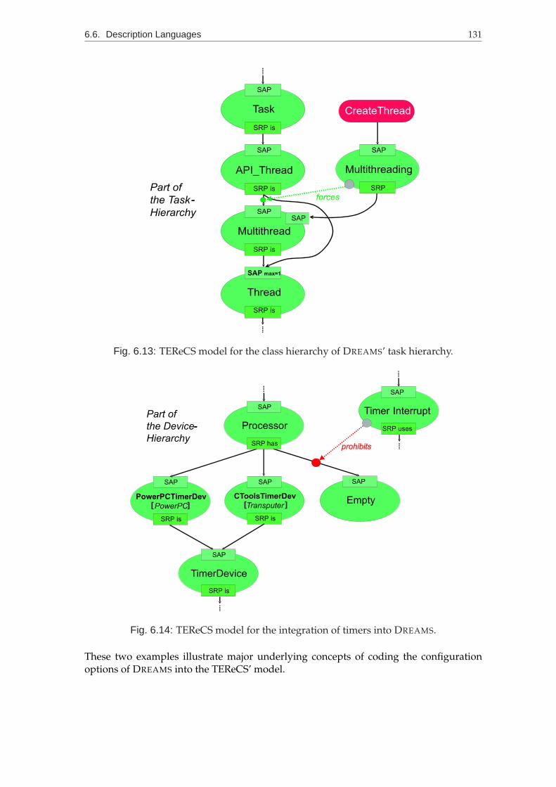
6.6. Description Languages 131
--
SAP
Part of
Task
API_Thread
Multithread
Thread
SRP is
SRP is
SRP is
SRP is
SAP
SAP
SAP max=1
SAP
the Task
Hierarchy
Multithreading
SRP
SAP
CreateThread
forces
Fig. 6.13: TEReCS model for the class hierarchy of DREAMS’ task hierarchy.
PowerPC[ ] [ ]
Processor
PowerPCTimerDev CToolsTimerDev
Transputer
TimerDevice
SRP has
SRP is SRP is
SRP is
SAP
SAP SAP
SAP
Empty
SAP
Timer Interrupt
SRP uses
SAP
prohibits
-
Part of
the Device
Hierarchy
-
Fig. 6.14: TEReCS model for the integration of timers into DREAMS.
These two examples illustrate major underlying concepts of coding the configurationoptions of DREAMS into the TEReCS’ model.

132 Chapter 6. TEReCS
6.7 Knowledge Transfer from the Application to the Configurator
This section tries to explain briefly in which way knowledge about the application canbe transferred to the configurator and in which way it can there be exploited for theoperating and communication system’s configuration. The requirements specification (asdescribed in Section 6.6124) defines the behaviour of the application. When this behaviouris known a priori, then the operating and communication system can be implementedappropriately. This means that specific services are implemented in such a way, so thatthey cope only with the required use case. They do not produce any overhead, becausethey need not to handle excluded use cases of the application. The code of a servicecan often be simplified, if assumed that special restrictions hold. These restrictions aredefined by the application programmer and are often directly intended. The restrictionsdefine a special behaviour of the application or they define that the application mustbehave in a special way.
An example is a specific scheduling scheme, which depends on the task set’s proper-ties. Another example is the synchronisation of a resource access. The synchronisationmust only be implemented, if the resource is really shared simultaneously between dif-ferent processes. If the resource is not shared or the resource is never accessed duringthe same time slot (implicit synchronisation), then the explicit synchronisation by usinga semaphore, for example, is not required. Additionally, if a resource is accessed only bytwo processes, then the synchronisation code can be simpler, as if it would be, when it isaccessed by an unknown number of processes.
Specific knowledge about the application is used during the configuration of the operat-ing systems in order to simplify the implementations of certain operating and commu-nication system services. Because of this additional knowledge about the behaviour ofthe application, the operating and communication system functionality can be adaptedto the special requirements of the application. Or, expressed from another point of view:The operating system specification is enriched by specifications about the application.Thus, this additional knowledge can be exploited for optimising the implementationsof operating and communication system services. This process of integrating additionalknowledge into the operating and communication system’s specification is a knowledgetransfer from the application’s domain into the operating and communication system’sdomain.
The configurator is responsible to integrate this additional knowledge correctly. InTEReCS the functional correctness of the generated operating systems is assured man-ually. The operating system designer, who integrates new services into the knowledgebase for operating system services (USG), must assure that these services correspond tothe other services and that they will only be selected, if the correct use case, for whichthe service had been developed, is applied. This can be done by the use of constraints.Often, virtual services, that represent those use cases, are defined and must explicitly beactivated by the use of primitives in the requirements specification. The activation ofthose “virtual” services control the correct selection of the other services by constraints.However, these constraints must be correctly defined by the operating system engineer.
In this way the knowledge about special use cases is integrated into the operating andcommunication system: The application demands for specific primitives that request for(virtual) services that again activate certain constraints, which control the correct selec-

6.8. Real-Time Analysis 133
tion of services from their alternatives. This is exactly the idea of puppet configuration (seeSection 5.4100).
Besides information about the application’s behaviour also information about the ex-pected temporal correct execution of the application is provided to the configurationprocess. This information comprises worst-case execution times of the processes, theirexpected maximum finishing and response times (deadlines) and the relative event times,when a process calls special operating system services. These relative event times aremeasured from the start of the process. During the configuration the implementation ofthose operating system calls (represented by the use of primitives) is determined. Theoverhead for each implementation of an operating system service is known, because ithad been also specified by the operating system engineer while he integrated that serviceinto the USG. To determine the overheads is not part of this thesis. Already existing tools,like CHaRy [1], can do that. These already known overheads are forwarded together withthe timing information of the application to a real-time analysis of the application’s be-haviour in co-operation with the operating and communication system’s behaviour (seeSection 6.8).
When the timing analysis detects failures of the timeliness behaviour (deadline misses),then mainly the configuration of some operating systems or the configuration of the com-munication system must change. This is mainly done by selecting other communicationpaths (change in routing) or other task mappings onto processors. In this way, the cre-ation of a functional correct configuration and the timing analysis is executed alternatelyunless both succeed or the configuration does not find any more valid configuration.
The process of the timing analysis is described in the next Section 6.8. Section 6.9142 andSection 6.10147 explain, in which way the configuration and the timing analysis interact.
6.8 Real-Time Analysis
For real-time analysis mainly two approaches exist. The first approach is the workloadanalysis, in which the cumulative workload of the processors, devices, and communi-cation links must not exceed 100% or even a lower limit. The second approach is theresponse time analysis, in which the overall sum of all delays of an action (including itsexecution) between the arrival of a request and the time to finish servicing it must notbe greater than the deadline. In this case all the possible orders of the delays (runs of aschedule) must be considered. Therefore, an analysis has to take care of all possible in-terruptions and disturbances in an execution path. For complex systems, and even morefor heterogeneous systems, this becomes very hard to solve. For example, in a communi-cation system, which consists of several different communication links, the transmissionand queuing delays differ. Moreover, if the protocols are different on the paths, then theblocking delays have to be calculated appropriately. Thus, the analysis has to cope witha lot of different formulas according to the path of the message.
Other problems for the analysis of distributed communicating processes are the mutualinfluences of the process scheduling and the communication delays. The process schedul-ing determines the relative and absolute times of sending and receiving events. Thisforms the basis of the calculation of the end-to-end communication delay. But the com-munication delays have again impact on the blocking delays of the process schedules.

134 Chapter 6. TEReCS
Thus we have a cyclic dependency. Real-time analysis often assumes that this will resultinto a stable state, where the mutual influences are broken. This means that a slightlydifferent process schedule does not change the blocking delays or vice versa. Often, real-time analysis assumes that the blocking times are independent of the schedule and, there-fore, they can be determined a priori. This results into worst-case timings for the blockingdelays, which are often too pessimistic (see PIP, PCP, SRP). In real-time analysis also theprecedence constraints between tasks are ignored or require a complex analysis scheme(see EDF∗ or Spring). But in this thesis precedence constraints due to communicationsare assumed to be absolutely indispensable for distributed embedded systems.
For this reason, in TEReCS another approach is followed. Assuming, that the executiondelays of all atomic actions can be calculated very precisely, and their order can also bedetermined precisely, then an execution model of the final application can be created.From this execution model all deadline misses can be observed. Additionally, if a dead-line miss occurs, then the actions responsible for delays can be identified. Consequently,if we have an execution model of all atomic actions, then their execution can be visualisedin form of a Gantt diagram. This can give a deeper insight into the application for theengineers. They can realise, what happens when on the target system. This approach issimilar to a simulation of the application.
In contrast to a simulation the code will not be executed or analysed. Control structures ofthe code, like condition statements or loops, will not be considered. Execution blocks aredefined instead. An execution block represents the execution time of a code sequence.All loops in the code are assumed to be unrolled. For a condition statement only oneexecution path is considered.
In order to achieve the schedule of the final execution, certain execution blocks mustbe arranged in the form of a schedule. This means that the execution blocks are placedchronologically onto the time line. An execution block can be interrupted by an event. Toeach event a certain sequence of other execution blocks is assigned. The occurrence ofan event means that the assigned sequence of execution blocks must be planned imme-diately. Thus, an execution block can be divided into interrupted sub-blocks, which wecall runs.
A process (task or thread) of the system is represented by one execution block. Each callof a primitive (system call) of the operating system or a real interrupt of a processor willbe interpreted as an event. Therefore, each execution block contains a time-ordered listof events. These events have to be planned relatively to the starting time of the executionblock. Each execution block can again invoke other events at its end. In this way a Time-triggered Event Scheduling of the execution blocks is realised. This is similar to the TTPapproach of Kopetz (see Section 4.4.2.384). The main difference is that the realisation (seeSection 6.8.4139) is not seen as strict as the TTP does.
In order to manage a distributed system consisting of parallel executing processors, foreach processor (CPU) one time line exists. Thus, for each processor a schedule of runswill be planned. For controlling the event flow, like operating systems do, an event willbe inserted into a time-ordered global event list, when it is invoked. But the occurrence ofthe event can be delayed into the future. Additionally, execution blocks can wait for cer-tain events to be present in that event list. An execution block, which waits for events, canonly be planned for a schedule, when the events are already in the event list and the time,when the events will occur, are reached. The event can only be taken (planned/executed),

6.8. Real-Time Analysis 135
when it is enabled and when there is an execution block, which waits for that event, inorder to be placed onto the schedule. For this reason the subsequent planning of execu-tion blocks can be interrupted, when events are missing. Such waiting execution blocksare inserted into a waiting list per processor. Besides the waiting list a ready list exists.Execution blocks that have to be planned are inserted into the ready list or waiting list ofeach processor accordingly.
The complete timing analysis is implemented by the tool TANA of TEReCS. In the follow-ing sections the execution model and the planning, respectively scheduling algorithm ofthe execution engine will be presented in detail.
6.8.1 Scheduling Model
First, we will define some basic items, which are used for the simple scheduling model.
ResourceNormally, each Resource contains a waiting queue, whose items (processes that wantsto access that resource) are ordered by a priority and by a FIFO ordering. For this schedul-ing engine the local waiting queues of all the Resources are integrated into one singleglobal waiting list (WL).
A Resource defines several Events that can be executed on this resource. For example,this can be up() or down() for the corresponding semaphore.
Whenever a Resource is defined, we also define the number of units available. Thisshall be referred to as the amount of resources available. These units can be produced andconsumed by signals() and waits() . A Resource can be disabled, which meansthat no units can be consumed thereafter.
All Resources must be placed onto a CPU or onto GLOBAL. A Resource can be placedsimultaneously on different CPUs and on GLOBAL. GLOBAL is an implicitely defined“virtual” CPU.
The following items of an execution model are derived from Resource :
• CPU – is representing a processor node of the network• Task – is representing a process or thread of the system• Semaphore – used for synchronisation of tasks• ComLine – used for communication between tasks• Timer – used for time management of tasks, like sleeping
Thereby, the scheduler of an operating system and also interrupts have to be modelled astasks.
EventAn Event can be called asynchronously by a Task . Each Event defines a sequence ofExecution Blocks that must be planned subsequently in the defined order when theEvent occurs. Thus, an Event delays the execution of a task .

136 Chapter 6. TEReCS
An Event is always part of a Task and is always executed on a Resource . The Eventnormally represents the execution of operating system services.
Execution BlockAn Execution Block is an instance, which can be planned for a schedule. Never-theless, an Execution Block can be preempted by another ready Execution Blockwith higher priority. Execution Blocks can define their own priority or inherit it fromthe Task that is calling the Event to which the Execution Block belongs.
CPU1
t1 t2
signal
Duration(l)
1) wait
3) disable
2) signalWait
4) killSignal
5) signal
6) enable
CPU1 or orther CPU
transfer(t)
t3
7) sync_starttime
Fig. 6.15: Illustration of timings and execution points of the signal handling for an exe-cution block
At the end of each Execution Block several signals() can be emitted. This meansthat they are inserted into a global pending signals queue. These signals have to beactivated immediately, or in the future. If a signal() is activated, then the items of theassigned Resource are increased by the specified amount.
At the beginning of each Execution Block several waits() can be defined to be con-sidered. A wait() consumes the specified amount of items of a Resource , which isassigned to that wait() . But items can only be consumed, if enough items are present(see Section 6.8.2 on the next page).
Additionally, at the beginning of each Execution Block some Resources can be dis-abled. At the end of an Execution Block some Resources can again be enabled.
Execution Blocks can be preempted by other Execution Blocks with higher pri-ority because of the occurrence of Events or signals() . Therefore, ExecutionBlocks are divided into Runs. An Execution Block is always part of an Event orTask .
RunA Run is the smallest instance that will be planned and mapped into a schedule. It isalways a part of an Execution Block .
The duration and, therefore, its ending time is explicitly not known, but must be calcu-lated by the scheduling engine (see Section 6.8.2 on the facing page).

6.8. Real-Time Analysis 137
A Run is terminated if its Execution Block ends or if another Execution Blockwith higher priority can consume all of its Waits and, therefore, preempts the actualRun. The preemption can only occur when a signal is emitted.
TaskA Task is derived from a Resource . By this the Task can wait for itself. This is requiredin order to simulate a sleep by waiting for itself.
The complete run-time of a Task is defined as one master Execution Block . The com-plete master Execution Block of the task can be split into several Runs. In-betweenthe Runs the Events of the Task occur. Before and after each Run of the Task only oneEvent of this Task is allowed to occur at a time. That means that there must not existtwo Events of the same Task , which have to occur at the same time.
All Tasks are modelled as periodic tasks. At the end of their Execution Block , theirexecution starts all over from the beginning. This helps in scheduling periodic tasks ortasks that loop forever. If a Task wants to terminate, then it has to wait forever for asignal.
6.8.2 Time-triggered Event Scheduling Engine
All ready Execution Blocks are maintained by the ready queue (RQ). If an ExecutionBlock has to be executed, then this Execution Block is marked ready and is insertedinto the ready queue of the appropriate CPU.
Before an Execution Block can be executed, all its waits() must match the availableunits of the Resources , which are assigned to that wait() . All waits() must be ful-filled. That means that all units of the Resources of all waits() for the ExecutionBlock are consumed or none of them. If they are consumed, then the ExecutionBlock is marked ready. If they cannot be consumed, then the Execution Block ismarked waiting and inserted into the waiting queue. Additionally, the Task , to which theExecution Block belongs, is marked blocked. A wait() matches, if and only if, thereare enough free units in the referred Resources and if the Resources are enabled.
If an Execution Block is completely executed, then all signals() defined for thisExecution Block must be emitted. That means that they are inserted into the globalqueue for pending signals (PS). If a signal() from this PS list has to be activated, thenall waiting Execution Blocks of the waiting list WL (and blocked Tasks ), which arewaiting for this signal() and that can receive enough units now, will be set to ready.
If there exists no active Event of a Task , then the master Execution Block of theTask has to be executed until the next Event occurs or the task terminates.
When an Event occurs, the Event is marked active. Then the next Execution Blockof this Event has to be executed and, therefore, that Execution Block must also bemarked ready. If an Event is marked active and none of its Execution Blocks can bemarked ready, then the Event is finished and deactivated.
An Execution Block is executed until it either terminates or the occurrence of asignal() of the PS queue. If the Execution Block is the master Execution Blockof a Task , then it possibly has to be executed until the occurrence of the next Event of
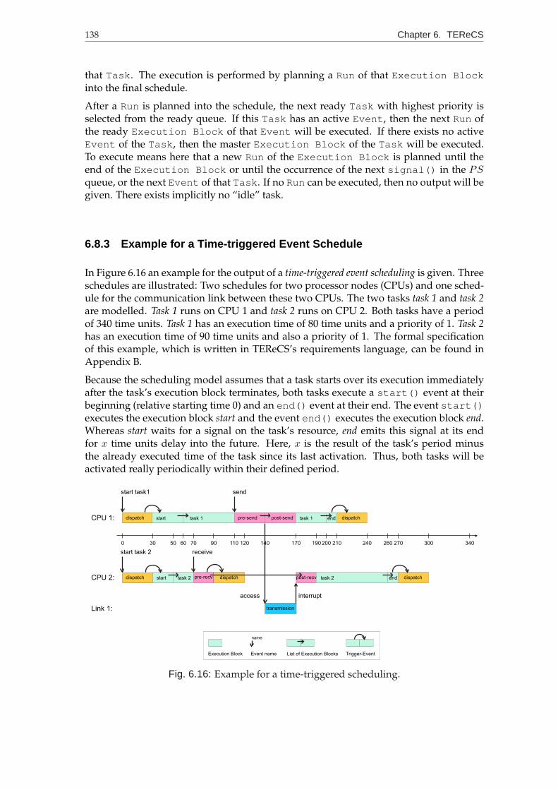
138 Chapter 6. TEReCS
that Task . The execution is performed by planning a Run of that Execution Blockinto the final schedule.
After a Run is planned into the schedule, the next ready Task with highest priority isselected from the ready queue. If this Task has an active Event , then the next Run ofthe ready Execution Block of that Event will be executed. If there exists no activeEvent of the Task , then the master Execution Block of the Task will be executed.To execute means here that a new Run of the Execution Block is planned until theend of the Execution Block or until the occurrence of the next signal() in the PSqueue, or the next Event of that Task . If no Run can be executed, then no output will begiven. There exists implicitly no “idle” task.
6.8.3 Example for a Time-triggered Event Schedule
In Figure 6.16 an example for the output of a time-triggered event scheduling is given. Threeschedules are illustrated: Two schedules for two processor nodes (CPUs) and one sched-ule for the communication link between these two CPUs. The two tasks task 1 and task 2are modelled. Task 1 runs on CPU 1 and task 2 runs on CPU 2. Both tasks have a periodof 340 time units. Task 1 has an execution time of 80 time units and a priority of 1. Task 2has an execution time of 90 time units and also a priority of 1. The formal specificationof this example, which is written in TEReCS’s requirements language, can be found inAppendix B.
Because the scheduling model assumes that a task starts over its execution immediatelyafter the task’s execution block terminates, both tasks execute a start() event at theirbeginning (relative starting time 0) and an end() event at their end. The event start()executes the execution block start and the event end() executes the execution block end.Whereas start waits for a signal on the task’s resource, end emits this signal at its endfor x time units delay into the future. Here, x is the result of the task’s period minusthe already executed time of the task since its last activation. Thus, both tasks will beactivated really periodically within their defined period.
300 50 60 70 90 120110 140 170 190 200 210 240 260 270 300 340
send
CPU 1:
CPU 2:
Link 1:
start task1
start task 2 receive
interruptaccess
dispatch dispatchdispatch
dispatchdispatch
start
start task 1 task 1
task 2 task 2
transmission
pre-send post-send
post-recvpre-recv
end
end
name
Execution Block Event name List of Execution Blocks Trigger-Event
Fig. 6.16: Example for a time-triggered scheduling.

6.8. Real-Time Analysis 139
In order to model a communication the resource Comline1 is defined. Comline1 declarestwo events, which can be executed: send() and receive() . The event send() exe-cutes sequentially the two execution blocks pre-send and post-send. The event receive()executes sequentially the two execution blocks pre-recv and post-recv. The execution blockpre-send emits at its end one signal on the resource Comline1. The execution block post-recvawaits this signal at its beginning. The signal will be delayed on the resource Comline1by 30 time units. This delay represents the media access time plus the transmission timeplus the response time of the receiving CPU.
Additionally, in this example it is specified that task 1 executes the send() event rela-tively after 50 time units. Also task 2 executes the receive() event after 20 time units.With this we have defined a communication between task 1 and task 2.
In order to model a Round-Robin scheduler of an operating system for both CPUs asecond task scheduler with the highest priority 0 and a period of 500 time units is defined.It specifies the execution block dispatch, which waits at the beginning for one signal on itsown resource and emits this signal at its end in order to generate its periodical execution.The duration of the execution block dispatch is 30 time units.
When the execution block post-recv has to be scheduled, but when no signal on the re-source ComLine1 is present, then post-recv has to wait and the execution block and its par-ent task will be blocked. Additionally, a signal without any delay will be sent to the taskscheduler of the same CPU. Therefore, we have defined a so-called wait-and-signal() ,which emits a signal, if and only if, the wait will result into a blocking. By this way, thetask scheduler can proceed immediately. The pending signal for the scheduler, which wassent by itself for its periodic activation, will be explicitly be consumed by the executionblock dispatch. With these definitions we attain that directly after the execution block pre-recv, the execution block dispatch is scheduled. This is because the post-recv is too early(the pre-send was not already done) and, therefore, post-recv must be blocked.
6.8.4 Schedulability Analysis
If all the durations of the execution blocks, the relative occurrences of the events, and thedelays of the signals, as well as the model of all tasks and their dependencies correspondto the reality, then the schedules will represent the original execution on the CPUs andlinks. But when only one timing is wrong, the complete schedule can be different (seeSection 6.10147). Thus, the finishing time of a task can be extremely delayed or shortened.
Taking the worst-case timings does not solve the problem, because the finishing time ofa task is not calculated upon worst-case assumptions. Under worst-case assumptions,like traditional real-time analysis does, the finishing time is calculated by considering allpossible worst-case delays. Here, only the worst-case timing of one, or a limited set ofspecific delays, is considered.
Nevertheless, in order to achieve good results for the timing analysis in TEReCS themodel is extended in the following way: Instead of one time for a duration, an eventoccurrence, or a signal delay, two times can be specified. These two times define an in-terval, in which the real event can happen. For this reason, the time-triggered schedulingmust be calculated for all times of this interval (because for each time the schedule canpossibly change). Moreover, if two intervals are given, then the schedules for all pairs of

140 Chapter 6. TEReCS
all time combinations must be calculated.
A schedule is considered to be feasible, if for all tasks, their finishing time is equal orlower than their deadline. This is the classical definition. A time interval is valid, if theschedules for all times of the interval are feasible. If more intervals are given, then allschedules for all combinations of times from these intervals must be feasible. This resultsinto the calculation of more than 2n schedules for n given intervals. (In fact, it wouldbe Πn
i=1mi schedules, where mi is the number of times that have to be considered perinterval i.) This would lead to an exponential run-time for the real-time validation.
To minimize the run-time for the timing validation, in TEReCS not all schedules will beconsidered. Only the schedules for the minimum and maximum times of the interval(the two specified limits) will be considered. The schedulability test will be done uponan heuristic, which estimates, whether another time in-between the interval can possiblychange the schedule or not. In this way, the run-time is still exponential, but the numberof considered schedules is really reduced to 2n schedules. If the heuristic schedulabilityanalysis with time intervals is used, then its result can be wrong. For this reason, thetime-triggered scheduling, which is used in TEReCS for the real-time validation, is – forthe first view – only an estimation for the timing validation, but it is not a proof for itscorrectness.
Nevertheless, it is a very practical approach. If the heuristic detects always a deadlinemiss, if and only if, such a deadline miss exists, then TEReCS’ timing analysis workscorrectly (see Section 6.8.4.1). So, the value of TEReCS’s timing validation depends on thequality of this heuristic function. In practice it could be shown that the defined functionachieves good results. But the real advantage of this approach is that the engineer, whoplans the system, can see the bottlenecks and timeliness arrangement of all modelledevents of the system. In this way he can gain additional information about the effects ofhis specifications onto the scheduling.
But TEReCS offers another advantage. The configurator of TEReCS can assure that thereal execution will be exactly that of the time-triggered scheduling. This will be achievedby integrating guards into the code for each event (system call). The guard is additionalcode, which assures that the event is taken at its expected absolute time. Eventually,the guard will delay the execution until the specified time is reached. Otherwise, if theestimated and expected time of the event was missed, the guard will complain and afall-back function can be activated. Thus, possible deadline misses can be detected muchearlier.
The execution time for the additional code of the guard, which is produced in orderto verify the event times, is considered during the time-triggered scheduling. But inTEReCS the guard for an event must explicitly be activated in the requirement specifica-tion. It is the engineer’s task to select appropriate events that should be guarded.
6.8.4.1 Heuristic Selection of Schedules
As already mentioned, whenever an interval is specified for the appearance of an eventor a delay, then all schedules have to be created. Each schedule implements the use ofone set of discrete times of the intervals. The purpose of the heuristic function is to selectone discrete time of the interval, for which the schedule has to be checked. Hereby, it is

6.8. Real-Time Analysis 141
essential to select a candidate, if possible, for which the schedule is not feasible. Then, anegative answer can immediately be issued and no further investigations are required.All schedules for an interval must be feasible, in order to allow that interval.
Before we describe the heuristic selection of schedules that have to be tested for feasibility,we define the direct and indirect influence of a time for a message transfer. If the timebelongs to any execution block that is executed by a sending task and that is executedbefore the real send of the message, then the change of this time can immediately changethe transfer time of the message, which is issued by that task. Then, this time directlyinfluences that message transfer of that task. The message transfer and the time alwaysbelong to the same sending task. If they belong to different tasks and additionally, thechange of the time changes the message transfer time, then the time indirectly influencesthat message transfer.
The heuristic function will make use of the following observations:
1. The end time of an interval will produce the maximum delay for the executing taskand the directly influenced receiving task.
2. The start time will produce the minimum delay for the executing task and the di-rectly influenced receiving task.
3. Any time of the interval can have impact on the delay of another task. Whether thisdelay will be extended or reduced for an earlier or later time, cannot be answered.
4. If for any two times the order of the messages of two communications on a mediachanges, then any time in-between these times will cause an interference betweenthose two communications.
5. For two times the order of a message between a directly influenced message and anindirectly influenced message can only change once. Here, during an hyperperiodcorresponding message transfers have to be considered.
From these observations we can derive the following: If for the schedules of the start andend time of an interval an interference between a directly and indirectly influenced mes-sage transfer exists, then the response time of the indirectly influenced message transferhave to be increased by the transfer time of the directly influenced message transfer. If thefinishing time of the receiving task, which receives that indirectly influenced message, isstill equal or lower than its deadline, then all of the schedules for all times of the intervalare regarded to be feasible. Otherwise a negative answer can be issued.
By this selection, only two times (the start and the end time) of a given interval must beconsidered. Of course, the run-time will be still exponential for the combinations of allstart and end times. But, (1) only two times per interval are considered, and (2) this isonly done for a positive answer.
Two rules help to prevent a lot of overhead:
1. Where possible, intervals should not be specified ⇒ less intervals reduce theamount of start and end time combinations.
2. An interval should be specified as small as possible ⇒ the probability of interfer-ences is less.

142 Chapter 6. TEReCS
These rules should be followed, when a requirement specification is created.
An advantage of this approach, which allows the definition of timing intervals, is thatbetween the schedules jitters can be observed.
6.9 Impact of the Configuration on the Timing Analysis
In this section we will demonstrate that the results of the estimated time-triggeredscheduling are often more accurate than those of a traditional worst-case analysis. Addi-tionally, we identify the influences of the configuration on the timing analysis by inspect-ing a few examples.
Task A Task B Task C Task D
CAN
Fig. 6.17: Hardware architecture and task mapping, where four tasks on four processornodes communicate via one single CAN bus.
We assume the following application scenario: The hardware of the target system is as-sembled of four homogeneous processor nodes, which are connected via four devices toone single CAN (Controller Area Network) [67] bus (see Figure 6.17). One general featureof a CAN bus is that the maximum size of a packet, which is sent over the bus, cannotexceed eight bytes. Therefore, messages often have to be split into several packets. Oneach of the four processor nodes one task runs. Task A sends a message to task B. Thismessage must be divided into four packets of maximum size. Task D sends a messageto task C by transmitting three packets. The run-time of task A without any operatingsystem overhead takes 32 time units. The run-time of task B takes 16 time units, thatof task C takes also 16 time units, and that of task D takes 24 time units. The operatingsystem call for sending a message (send event) is assumed to occur 13 time units aftertask A has started its execution. For task D this send event is assumed to be after 17 timeunits. The receive events for the tasks B and C are both assumed to be after 8 time units.The requirement specification looks like the following:
Task A : CA = 32, Esend(A) = 13Task B : CB = 16, Erecv(B) = 8Task C : CC = 16, Erecv(C) = 8Task D : CD = 24, Esend(D) = 17
Communication 1 : Task A −→ Task B with nA,B = 4 packetsCommunication 2 : Task D −→ Task C with nD,C = 3 packets
During the configuration of the operating systems for all four processor nodes the con-figurator determines the overhead of the operating system for the sending and receiving

6.9. Impact of the Configuration on the Timing Analysis 143
of these messages. The execution time for the system call send (send primitive) has to besplit into four phases. During the first phase the message is split and prepared for thetransmission. This phase has a duration of 7 time units. After this, each of the packetsis sent in the second phase by a device driver call, which takes 2 time units. After thecomplete message is sent an interrupt of the device driver, which lasts for 5 time units,informs the operating system in the third phase to proceed the sending task. In the fourthphase the operating system call needs for this 8 time units before the sending task is re-activated. Thus, the complete operating system overhead for sending n packets takes7 + (n ∗ 2) + 5 + 8 time units. The system call for receiving of a message (receiving prim-itive) is similarly split into such four phases. The complete operating system overheadfor receiving n packets takes 13 + (n ∗ 2) + 5 + 8 time units. The configurator gives thefollowing operating system overheads, which had been assigned by the operating systemexpert to the appropriate services:
OvhSys[pre-send] = 7OvhSys[dd-send](n) = 2n
OvhSys[irq-send] = 5OvhSys[post-send] = 8OvhSys[pre-recv] = 13
OvhSys[dd-recv](n) = 2nOvhSys[irq-recv] = 5
OvhSys[post-recv] = 8
OvhSys[send](n) = OvhSys[pre-send]+OvhSys[dd-send](n)+OvhSys[irq-send]+OvhSys[post-send]
OvhSys[recv](n) = OvhSys[pre-recv]+OvhSys[dd-recv](n)+OvhSys[irq-recv]+OvhSys[post-recv]
The physical transmission timeϕpacket for a packet of 8 bytes on the CAN bus is calculatedupon the bit rate and takes 6 time units. The overall transmission delay ϕsendtrans for npackets for a sending task lasts for (n − 1) ∗ 2ϕpacket time units. The sending task has towait only for (n− 1) packets to be transmitted. This is defined by the final configurationarchitecture of the operating system’s implementation. For the receiving task the overalltransmission delay ϕrecvtrans for n packets takes n ∗ 2ϕpacket time units, because the driverhas to wait for the reception of all packets. The transmission delays are worst-case values,because the transmission delay for each packet is assumed to be twice of the physicaltransmission delay. This is, because potentially the transmission of a packet must bedelayed by the media access, while actually another packet is on the bus.
ϕpacket = 6ϕsendtrans(n) = (n− 1) ∗ 2ϕpacketϕrecvtrans(n) = n ∗ 2ϕpacket

144 Chapter 6. TEReCS
A traditional worst-case analysis normally does not consider the times of the appearancesof the system calls. Simply the worst-case delays and execution times are summed. Forthe classical worst-case approach we obtain the following results:
RA = CA +OvhSys[send](nA,B) + ϕsendtrans(nA,B) = 96RB = CB +OvhSys[recv](nA,B) + ϕrecvtrans(nA,B) +RA = 194RC = CC +OvhSys[recv](nD,C) + ϕrecvtrans(nD,C) +RD = 158RD = CD +OvhSys[send](nD,C) + ϕsendtrans(nD,C) = 74
The finishing times for the receiving tasks B and C contain the finishing times for theirsending tasks. This has been done, because of the in-out dependency between a receivingand a sending task. For the classic worst-case analysis (e.g. see EDF∗ on page 70) thesending task is assumed to finish, before the message is transferred to the receiving task,which then can start its execution.
These results of the classical analysis can dramatically be improved, if the times, whenthe send and receive events occur, are considered. Especially, the response times of thereceiving processes can be calculated more accurate. In fact, the destination process cancontinue its execution, when the process received the message. This time also depends onthe time when the source process sends the last packet. For this reason, the time until thedata are received have to be calculated as the maximum of either the destination process’execution time til the receive event plus n times of the time that is spent for the devicedriver’s receive interrupt. Or it has to be calculated as the time of the source process’execution time til the send event plus the overall transmission delay ϕsendtrans for a sendingtask plus the time that is spent for the device driver’s receive interrupt:
R′B = max(Erecv(B) +OvhSys[pre-recv] +OvhSys[dd-recv](nA,B) ,Esend(A) +OvhSys[pre-send] + ϕrecvtrans(nA,B)+OvhSys[dd-send](nA,B) +OvhSys[dd-recv](1) )
+OvhSys[irq-recv] +OvhSys[post-recv] + (CB −Erecv(B))= 99
R′C = max(Erecv(C) +OvhSys[pre-recv] +OvhSys[dd-recv](nD,C) ,Esend(D) +OvhSys[pre-send] + ϕrecvtrans(nD,C)+OvhSys[dd-send](nD,C) +OvhSys[dd-recv](1) )
+OvhSys[irq-recv] +OvhSys[post-recv] + (CC − Erecv(C))= 89
These results can again be improved, if considered that the device driver’s sending inter-rupt will be executed parallelly to the media access delay:
ϕrecvtrans′′(n) =
{n ∗ 2ϕpacket : OvhSys[dd-send](1) ≤ ϕpacketn ∗
(ϕpacket +
⌈OvhSys[dd-send](1)
ϕpacket
⌉ϕpacket
): OvhSys[dd-send](1) > ϕpacket
R′′B = max(Erecv(B) +OvhSys[pre-recv] +OvhSys[dd-recv](nA,B) ,Esend(A) +OvhSys[pre-send] + ϕrecvtrans
′′(nA,B)+OvhSys[dd-recv](1) )
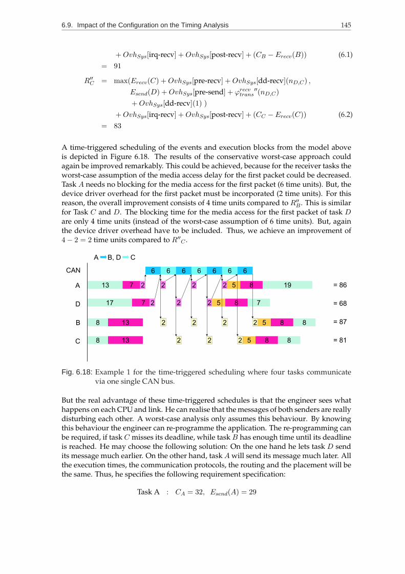
6.9. Impact of the Configuration on the Timing Analysis 145
+OvhSys[irq-recv] +OvhSys[post-recv] + (CB − Erecv(B)) (6.1)= 91
R′′C = max(Erecv(C) +OvhSys[pre-recv] +OvhSys[dd-recv](nD,C) ,Esend(D) +OvhSys[pre-send] + ϕrecvtrans
′′(nD,C)+OvhSys[dd-recv](1) )
+OvhSys[irq-recv] +OvhSys[post-recv] + (CC − Erecv(C)) (6.2)= 83
A time-triggered scheduling of the events and execution blocks from the model aboveis depicted in Figure 6.18. The results of the conservative worst-case approach couldagain be improved remarkably. This could be achieved, because for the receiver tasks theworst-case assumption of the media access delay for the first packet could be decreased.Task A needs no blocking for the media access for the first packet (6 time units). But, thedevice driver overhead for the first packet must be incorporated (2 time units). For thisreason, the overall improvement consists of 4 time units compared to R′′B . This is similarfor Task C and D. The blocking time for the media access for the first packet of task Dare only 4 time units (instead of the worst-case assumption of 6 time units). But, againthe device driver overhead have to be included. Thus, we achieve an improvement of4− 2 = 2 time units compared to R′′C .
13
17
8
8 13
19
77
6 6 6
2 2 8 8
2 2
5
852
13 8852 2 2 2
6
7
6 6 6
2 2 2 5 82
= 68
= 86
= 87
= 812
A
CAN
D
B
C
A B, D C
Fig. 6.18: Example 1 for the time-triggered scheduling where four tasks communicatevia one single CAN bus.
But the real advantage of these time-triggered schedules is that the engineer sees whathappens on each CPU and link. He can realise that the messages of both senders are reallydisturbing each other. A worst-case analysis only assumes this behaviour. By knowingthis behaviour the engineer can re-programme the application. The re-programming canbe required, if task C misses its deadline, while task B has enough time until its deadlineis reached. He may choose the following solution: On the one hand he lets task D sendits message much earlier. On the other hand, task A will send its message much later. Allthe execution times, the communication protocols, the routing and the placement will bethe same. Thus, he specifies the following requirement specification:
Task A : CA = 32, Esend(A) = 29

146 Chapter 6. TEReCS
Task B : CB = 16, Erecv(B) = 8Task C : CC = 16, Erecv(C) = 8Task D : CD = 24, Esend(D) = 1
Communication 1 : Task A −→ Task B with nA,B = 4 packetsCommunication 2 : Task D −→ Task C with nD,C = 3 packets
Because the same tasks will send the same messages, the configurator will give the sameoperating system overheads. With this inputs the worst-case analysis of Formula 6.1 and6.2 will yield to:
R′′B = 107R′′C = 67
The time-triggered scheduling achieves much better results (R′′′B = 91, R′′′C = 55), whichare taken from Figure 6.19. The calculated finishing times of the tasks are much better,because the worst-case assumption that a media access delay is as long as a completemessage transfer time (6 time units) need not to be considered for this example. We caneasily observe that no packet will be delayed, because the transmissions take place atdifferent time intervals.
= 78
= 91
= 62
= 55
A
CAN
D
B
C
A B, D C
Fig. 6.19: Example 2 for the time-triggered scheduling where four tasks communicate viaone single CAN bus, but the event of the second communication starts muchearlier.
We can summarise that the configuration determines the following inputs for the timinganalysis:
• Implementation of system calls (primitives)
– Protocol and/or device driver that is used
– Sequence of execution blocks to be executed per primitive
– Duration of primitive (operating system overhead)
• Routing
– Resource usage

6.10. Impact of the Timing Analysis on the Configuration 147
It should clearly be stated that TEReCS, in fact, determines the primitive implementationfrom a set of a priori defined ones. These primitive implementations including the se-quence and duration of their execution blocks for the timing analysis had been definedby operating system experts for different use cases. They had been integrated into theUSG. TEReCS determines the correct use case upon the overall primitive usage of thecomplete application (see “Puppet Configuration” in Section 5.4100) and some side con-straints. Each primitive implementation is assigned a sequence of pre-defined executionblocks. Thus, TEReCS need neither to invent new execution blocks nor their sequence.TEReCS only selects the appropriate pre-defined set. This means that the sequence andduration of the execution blocks have to be defined in advance by the operating systemexperts (see Section 6.4.1113).
6.10 Impact of the Timing Analysis on the Configuration
The results that are received from the previously presented time-triggered event schedulingof execution blocks have –of course– impact on the generation of a final configuration forthe operating and communication system.
In the last example of the previous section (see Figure 6.19) the finishing time of thereceiver task B was extremely prolonged, because the send event of task A was nearlymoved to its end. For this reason, task B can miss its deadline.
Let us now additionally specify that a RS-232 peer-to-peer link exists between the pro-cessor nodes on which task C and D are placed (see Figure 6.20). Assume also that therequirement specification is the same as in the first example on page 142.
Task A Task B Task C Task D
CAN
RS-232
Fig. 6.20: Hardware architecture and task mapping, where four tasks on four processornodes communicate via one CAN bus and one serial RS-232 peer-to-peer con-nection.
First, the router module of the TEReCS’ configurator will map all communications ofthe example onto the CAN bus (because it is the fastest link). Thus, the timing analysisbased on the time-triggered scheduling will receive the results from Figure 6.19. Let usassume again a deadline miss of task B. For this reason, the configuration has to bechanged. This is primarily done by mapping other communications, which delay taskB,onto other communication links if possible. In that example task B will be delayed bythe communication between task C andD. But for exactly this communication the routercan choose the other path via the RS-232 link. Thus, the configuration is again started,where it is prohibited to map the communication between task C and D onto the CANbus. As a consequence the routing will change. Also the operating system overhead

148 Chapter 6. TEReCS
and the protocol will change for the communication between task C and D. The time-triggered schedules for the new configuration are depicted in Figure 6.21. The finishingtimes of all tasks are decreased; but unfortunately, more resources have to be spent forthe configuration.
= 86
= 87
= 68
= 81
A
CAN
Serial
D
B
C
A B, D C
Fig. 6.21: Example 3 for the time-triggered scheduling where four tasks communicatevia one CAN bus and one serial RS-232 connection.
This example shows in which way the timing analysis influences the configuration pro-cess. In order to exploit this feature, a lot of communication links have to be specified forthe target hardware. The configuration process tries to use only a minimal set of theselinks for the application’s communications. Which link has to be chosen first is deter-mined by giving costs to each link. These can be direct or indirect costs. Direct costs canbe, for instance, the price of the hardware. Indirect costs are produced by the softwareservices that have to be selected in order to manage the link.
As we have seen, an additional link is used, if a communication that produces a deadlinemiss must be newly routed. In TEReCS communications are distinguished that directlyor indirectly produce a deadline miss. A communication directly causes the deadlinemiss, if, for instance, the communication is between tasks A and B and task B misses itsdeadline. The communication indirectly causes a deadline miss, if the communicationis between task A and B, but it delays another communication between tasks C and D,so that task D misses its deadline. When a deadline miss occurs, first a communicationthat directly causes the miss is tried to be re-mapped. If this is not possible or does notachieve success, then the communications that indirectly cause the miss are tried to bere-mapped.
In this way, TEReCS can determine the minimal set of required communication linksbetween the processor nodes. TEReCS implements and routes all communications insuch a way that they do not cause a deadline miss of any task. But obviously, this can beimpossible, if there are not enough resources available.
The routing of all communications is one main part of the final configuration. Whereasthis is nearly done automatically in TEReCS, the mapping of the tasks onto the processornodes must manually be done by the engineer. But when no solution can be found, theengineer can identify tasks from the time-triggered schedules, which can be re-mappedonto other processors in order to eliminate a resource overload condition.
6.11. Contribution of the Chapter 149
Besides the automatic communication link selection, the routing, and the manual taskmapping, also parameters, properties, or modes of the communication links can be de-termined. For example, the baud-rate should be selected for a RS-232 serial peer-to-peerlink. This can be done in TEReCS by specifying two RS-232 links between the same pro-cessor nodes, where one link transmits the bits with, for instance, 9600 Baud and thesecond link uses 38400 Baud. If a lower baud-rate is preferred (because the link is thenless susceptible to electro-magnetic disturbances), then the link with the lower baud-rateshould cause lower direct costs.
In the same sense as TEReCS selects the appropriate communication links, TEReCS se-lects appropriate devices in order to access the links from the processors. For instance,the devices for a CAN bus access vary in their performance and, therefore, also in theircosts.
Besides these more or less direct influences of the timing analysis onto the final con-figuration, there also exists indirect influences. Indirect influences have impact on theoperating system of a processor node. This is obvious, since the change of a communi-cation link and/or a device means also to change the device driver inside the operatingsystem. But, additionally, the access to the device can change. That means, for instance,the access must be protected, if more than one task uses simultaneously the driver. Orthe buffering scheme for the messages must change, because the messages have the sameor different priorities. Also the buffer size depends on the number of messages that aremapped onto a certain connection. All these indirect impacts on the software architecturechange the operating system’s overhead. This can also help to find a feasible scheduleover all processors.
We can summarise that the timing analysis has the following influences on the final con-figuration:
• Direct impacts:
– Prohibiting certain communications to be mapped onto specific links and/ordevices (−→ automatic re-routing)
– Manual re-mapping of tasks onto processors
• Indirect impacts:
– Parameter or mode changes of the links and devices– Change of the software architecture of the operating system– Change of the overhead of the operating system services
These impacts represent some of the main advantages of TEReCS. TEReCS determines avalid communication system, which means that all communications and, therefore, alsothe tasks can feasibly be scheduled. For this reason, the appropriate links, devices, andoperating system services per processor are selected, respectively configured.
6.11 Contribution of the Chapter
In this chapter we have presented a new methodology for the automatic configurationof operating and communication systems. Atomic services of the operating systems can

150 Chapter 6. TEReCS
be included or excluded from the final implementations. This is primarily done to savememory. Also, there exists multiple implementations for the same service. Each serviceimplementation is only applicable to a specific use case. Thus, the lack of a service Acan result to force service B to be implemented in a special way. Or, it is known thatthe application behaves in a certain way, then a service C can ignore a special use caseand may be implemented more efficiently. By this way, the integration of applicationspecific knowledge about its behaviour into the operating system can save memory forthe services’ implementation as well as execution overhead. The approach that is usedhere is named “Puppet Configuration”.
Similar benefits can be achieved for the communication system. It is the task of the con-figuration process to determine the routing of the messages through the network and tointegrate or exclude link device drivers into the appropriate operating system of eachnode. The routing tables have to generated and the existing device drivers must be pa-rameterised (address, port, protocol, access protection, etc.). It is also the task of theconfiguration process to determine the minimal required links of the network, so thatthe timeliness transfer of all messages is just possible. Because we assume to have a dis-tributed real-time application, the check for deadline misses must be done. Therefore,TEReCS has also integrated a verification tool for the timeliness execution of all commu-nication tasks. The maximal communication end-to-end delays are determined as wellas the schedules of all the messages on the media and of all the processes on the nodes.This is done by a so-called “Time-triggered Event Scheduling”.
The configuration algorithm of TEReCS follows a structure-based approach. In fact theknowledge base representation is modelled as an AND/OR-DAG with a top-down con-cept. It supports for constraints, which are in TEReCS a powerful mechanism to deter-mine the correct choice for alternative implementations upon a specific use case. Themodel also supports the specification of parameters, which are used for a concrete selec-tion. The Puppet Configuration approach assumes that (due to the constraints) only validand functionally correct configurations can be generated. Thus, only the real-time as-pect must be verified. The configuration works without user interaction and, therefore,is automatic. The user only has to provide a requirements specification of the applica-tion. Operating system details are completely hidden from the user. The configurationalgorithm implements a design space exploration of the operating system under consid-eration. The modelled graph is traversed and the selection of alternative paths are madeupon a cost function and the constraints. Here, the graph is traversed in a top-downmanner for each required primitive to the required hardware. For the communicationservices the routing is considered. Here, also hops for messages in a multi-hop networkmay occur. The graphs of each node of a message path is traversed accordingly fromthe send primitive to a device, from a device to another device, or from the device to thereceive primitive.
The configuration model and also the configuration algorithm allow hierarchy. There-fore, a graph can be clustered. A cluster represents a sub-graph and appears to be a sim-ple service node in the graph of the next hierarchy level. By this way, the complexity of agraph can dramatically be reduced. Additionally, this supports a faster re-configuration.If the requirements specification is only slightly changed, then only those cluster-graphshave to be re-configured that are involved into those changes. This is especially true forthe configuration loop of the configuration and analysis phase. The hierarchy also helpsto minimize the memory that is used during the configuration. A cluster-graph, which

6.11. Contribution of the Chapter 151
is not selected, must not be loaded for the configuration into the memory (informationhiding). Another advantage of the clustered hierarchy is that it can help to steer the con-figuration algorithm. When the clustering and, therefore, also the hierarchy is calculatedjust before the configuration. Then also the requirements specification can be integrated.Thus, different requirements specifications can lead to different clusterings, which mayresult into different configuration runs.
The primary goal of the Time-triggered Event Scheduling for the timing analysis is to check,whether all tasks meet their deadlines. The aspects of considering distributed commu-nication systems and the configuration itself arise some problems that are often ignoredin the classical and theoretical timing analysis. Precedence constraints have to be consid-ered due to the complex in/out-dependencies. Also the resource access constraints onthe links (media access) result into unknown blocking delays. Their calculation is verycomplex and is often very pessimistic. These reasons make the analysis quite complexand lead often to very pessimistic assumptions. Additionally, the classical timing anal-ysis ignores the system overhead (task switching, etc.). But in TEReCS it is essential toincorporate this, because it can change due to different configurations. That means thatthe configuration has impact on the timing of the system. A solution for this problem waspresented in form of the optimistic Time-triggered Event Scheduling scheme. Although theresults of that analysis may not exactly reflect the real task execution, they can give hintsfor the detection of bottlenecks in the system. However, by the integration of event guardsthe execution can follow the time-triggered approach and will match the analysed sched-ules. Additionally, the possibility to define event intervals, the heuristic evaluation, andthe very exhaustive search (exponential) on all possible schedules achieves in practicegood results. They are seldomly too optimistic.

152 Chapter 6. TEReCS

CHAPTER 7
Results
Currently, DREAMS consists of about 280 classes out of which about 100 classes are cus-tomisable class skeletons. These led to approximately 200 services that are modelled withabout 220 SAPs and 300 SRPs. The reason for having twice more services than skeletonsis based on the fact that every Skeleton has an API (Application Programming Interface)symbol, which defines the access interface to that type of skeleton. This complexity makesit quite difficult to create manually a good and working configuration. TEReCS can man-age this very easy. A user of DREAMS need not to be an expert for all of the configurationitems of DREAMS.
After modelling DREAMS several application scenarios with different demands to theoperating system were defined. These scenarios include different memory managementstrategies and use or exclude interrupt facilities, multi-threading, multiplexing of sharedresources, local or external communication, debugging facilities, terminal output, etc.,on different hardware architectures. The resulting configurations for each scenario werevalid and no mal-configurations could be detected by an “expert” for DREAMS. On thecontrary, some configurations were better than manually made ones. There were somesurprising decisions of which the expert had not thought of, but led to better implemen-tations.
Moreover, the configuration was developed nearly 120 times faster than doing it manu-ally (in the worst-case the manual configuration needs approx. 60 min; automatic approx.30 sec). Additionally, it could be verified that the target code size of the systems variedvery much. The minimal system reached a size of about 2.4 KBytes whereas the biggestone (using all features of the system) required about 150 KBytes of memory for code anddata. Both systems were made for a 32 Bit processor (PowerPC). This shows impressivelythe great impact of configuration on the size of the system. Likewise, it is expected thatthe execution time also differs much [43]. Therefore, a demonstration scenario had beendeveloped. The communication system had been configured differently (mainly by usingother protocols). The end-to-end delay of a communication and the service intervals hadbeen measured by software monitors.

154 Chapter 7. Results
7.1 Demonstrator
In order to measure quantitative benefits of the operating and communication system’sconfiguration, DREAMS was extended by special customisable options. For the test sce-nario the rapid-prototyping hardware USAP from the ETAS GmbH, Germany, was used.This hardware comprises a 19 inch rack with power-supply and a proprietary backplaneand up to 6 extension slots. It is extended by 4 processor boards that are equipped witha 20 MHz PowerPC 604 with 8 MBytes DRAM memory in combination with a 10 MHzTransputer T805 with an extra 1 MByte SRAM. The 8 MBytes DRAM are implementedas shared memory between the two processors. The backplane connects the Transputersof each slot in a sequential manner. The first slot is equipped with a single TransputerT405 and only 256 KBytes of memory. One of the links of this Transputer can be reachedfrom outside, for example, from a host system. The hardware topology of this system isdescribed in TEReCS’ notation in Figure A.1166 in Appendix A.
DREAMS can actually be customised to run on Transputers and on PowerPC 60x, Pow-erPC 509, and PowerPC 555. The communication system supports for Transputer links,for serial RS-232 interfaces, like the TL16C552A chip (used in the PowerPC 509) or theSCI (Serial Communication Interface) of the PowerPC 555, for CAN devices, like the onewhich is used in the PowerPC 555 chip, and for a shared memory interface in order toexchange messages. Device drivers for these devices can be integrated accordingly to theusage and present hardware. The device driver can be enabled or disabled to listen forincoming messages. The listening for each device is implemented as a virtual interruptservice routine. An optional routing service can be integrated into the operating system,which selects the appropriate outgoing device upon a routing table. The routing serviceis implemented as a single task. Incoming messages will be redirected to the internalmailboxes, if addressed, or to the routing service, if present. Each communication de-vice, each mailbox and the routing service are implemented as ports, which provide aunified message exchange interface. This provides for universally connected ports. Thus,the in-port of a communication device can be connected directly to the out-port of aninternal mailbox, to another communication device, or to the routing service. Each portcan be implemented as a resource or not. When the port is implemented as a resource,each access (of send() and receive() ) is protected by a semaphore (mutual exclusion).
For the serial links (Transputer and RS-232) three different protocols are alternativelyselectable:
Generic. The first protocol variant is a generic protocol. It transfers a header before theuser data (message body) are transmitted. The header contains information aboutthe destination node, the destination mailbox, and the size of the user data. Theheader’s size and structure is fixed. The size of the user data can vary, but must bea multiple of one byte. The header can be received asynchronously to the messagebody. But each user data must be preceded by one header. Thus, after receiving aheader, the memory for the user data (which can be of different size) are allocatedin order to store and forward the message.
Maximum Size. The second protocol variant transmits the header and body at once asone packet. Both must be received in one stream. The size of the packet and, there-fore, also of the message (user data) is constant per link. The header also contains

7.1. Demonstrator 155
448
send
sendHsendD
recvH recvD
sendwait
link requesthandle
malloc deliver
probe receive
t
PPC1
PPC2
TP 1
TP 2
SMI
SMI
Link Link
41 21
38 78
40
109112
30
A all times in µsec
Fig. 7.1: Measured schedule for the transfer of 64 Bytes user data over four processornodes. The Transputer link must be requested and the Generic protocol is used.
a size field, because the user data of the message can be less than the size of thepacket’s body. The advantage is, that the memory for a message can be allocatedasynchronously before a packet is received. Additionally, the sender must not ac-cess the media twice: for the header and for the body. The send delay will dramat-ically be reduced.
Constant. The third protocol variant does not transmit any header before the user dataare sent. This assumes that each received packet has the same destination, which isstatically known, and always has the same size.
Other protocols (like mixtures of these protocol variants) can possibly be requested; butare actually not implemented. The configuration for each node of the target system mustdetermine the following items:
• Processor type• List of the required communication devices that defines per device:
– Identifier
– Type
– Base address
– Boolean flag for the resource protection
– The protocol variant that is to be used for the send() and receive() meth-ods
– The local out-port to which the in-port of this device is connected
• Routing table which contains for each destination (node or channel identifier) thelocal outgoing device identifier
These things are automatically determined by the configurator tool TGEN of TEReCS forDREAMS. This comprises especially, whether all messages that are sent via one specificlink have a maximum or fixed size and, additionally, have the same destination. Thus,one of the three protocol variants can be selected. Whether the communication deviceis used exclusively by one task or whether it is used simultaneously by multiple tasks is

156 Chapter 7. Results
336
send
sendHsendD
recvH recvD
sendwait
handle
malloc deliver
probe receive
t
PPC1
TP 1
TP 2
SMI
SMI
Link Link
41 21
38 78
40
109
30
PPC2
Ball times in µsec
Fig. 7.2: Measured schedule for the transfer of 64 Bytes user data over four processornodes. The Transputer link is not requested and the Generic protocol is used.
noticed (interrupt service routines are also seen as tasks). Thus, the resource protectioncan be selected or removed. All these things are described within alternatives of theURSG.
It is also recognised that all messages that are received from the same in-port must possi-bly be redirected to the same local out-port. This means that the in-port will be connectedto that out-port or, if they do not have the same destination, it will be connected to theout-port of the routing service. It is also recognised that all messages that have to be sentvia one out-port have a maximum or fixed message size. For these reasons, the protocolvariant can be determined to be chosen.
For the example a task A on the PowerPC 5 wants to transmit 64 Bytes of user data tothe task B on the PowerPC 3 (see Figure A.1166 and Figure A.3175). Therefore, the datamust be routed via the shared memory interface (SMI) to the board’s communication proces-sor, which is the Transputer 4. This Transputer has to forward the data to its neighboringTransputer 2, which then stores the message. The message is stored here, because it has tobe delivered via the SMI to its assigned PowerPC 3. When the taskB wants to receive the
306
send
sendHsendD
recvH recvD
sendwait
handle
malloc deliver
probe receive
t
PPC1
TP 1
TP 2
SMI
SMI
Link Link
41 21
38 78
40
79
30
PPC2
C all times in µsec
Fig. 7.3: Measured schedule for the transfer of 64 Bytes user data over four processornodes. The Transputer link is not requested and the Maximum Size protocol isused.
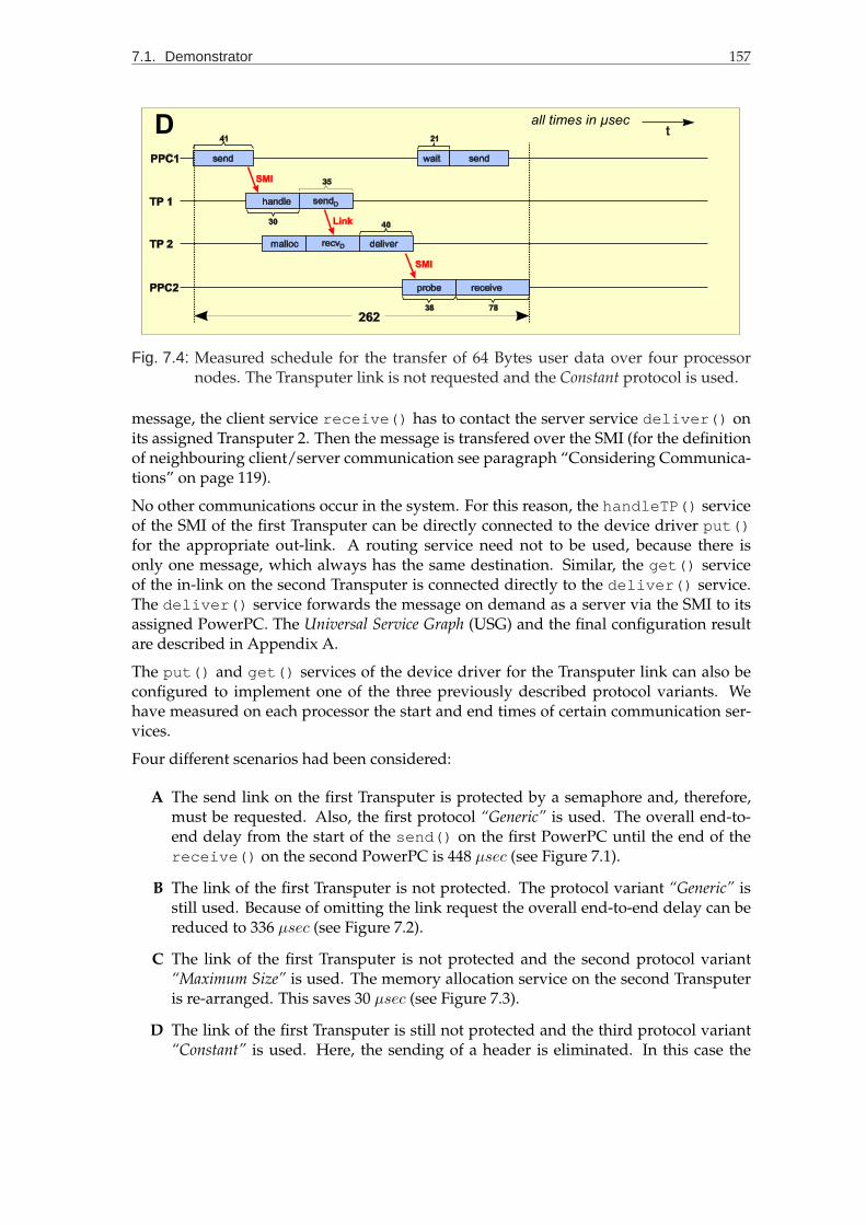
7.1. Demonstrator 157
262
send
sendD
recvD
sendwait
handle
malloc deliver
probe receive
t
PPC1
TP 1
TP 2
SMI
SMI
Link
41 21
38 78
40
35
30
PPC2
D all times in µsec
Fig. 7.4: Measured schedule for the transfer of 64 Bytes user data over four processornodes. The Transputer link is not requested and the Constant protocol is used.
message, the client service receive() has to contact the server service deliver() onits assigned Transputer 2. Then the message is transfered over the SMI (for the definitionof neighbouring client/server communication see paragraph “Considering Communica-tions” on page 119).
No other communications occur in the system. For this reason, the handleTP() serviceof the SMI of the first Transputer can be directly connected to the device driver put()for the appropriate out-link. A routing service need not to be used, because there isonly one message, which always has the same destination. Similar, the get() serviceof the in-link on the second Transputer is connected directly to the deliver() service.The deliver() service forwards the message on demand as a server via the SMI to itsassigned PowerPC. The Universal Service Graph (USG) and the final configuration resultare described in Appendix A.
The put() and get() services of the device driver for the Transputer link can also beconfigured to implement one of the three previously described protocol variants. Wehave measured on each processor the start and end times of certain communication ser-vices.
Four different scenarios had been considered:
A The send link on the first Transputer is protected by a semaphore and, therefore,must be requested. Also, the first protocol “Generic” is used. The overall end-to-end delay from the start of the send() on the first PowerPC until the end of thereceive() on the second PowerPC is 448 µsec (see Figure 7.1).
B The link of the first Transputer is not protected. The protocol variant “Generic” isstill used. Because of omitting the link request the overall end-to-end delay can bereduced to 336 µsec (see Figure 7.2).
C The link of the first Transputer is not protected and the second protocol variant“Maximum Size” is used. The memory allocation service on the second Transputeris re-arranged. This saves 30 µsec (see Figure 7.3).
D The link of the first Transputer is still not protected and the third protocol variant“Constant” is used. Here, the sending of a header is eliminated. In this case the

158 Chapter 7. Results
overall end-to-end delay takes only 262 µsec (see Figure 7.4).
These examples show impressively that the communication delay can dramatically beinfluenced by different configurations due to different application scenarios. It is the taskof the configuration process to determine the best implementation by considering theapplication’s behaviour.
These examples only consider the serial link communication of the Transputers. How-ever, this example can directly be applied to a serial RS-232 communication and it canbe adapted to other communication devices with other protocol variants. For instance,when a CAN bus is considered, protocol variants with and without message fragmenta-tion can be assumed, etc.

CHAPTER 8
Conclusion
The tool suite that has been developed for TEReCS consists of the configurator TGEN, thetiming analyser TANA, the creator TCLUSTER for the creation of a requirement specificcluster hierarchy and its configuration with TGEN, the editor TEDIT for the maintenanceof the URSG and RG, and the design tool TDESIGN, which implements TEReCS’ designcycle. TDESIGN calls TGEN and TANA until a valid configuration could be found. TDE-SIGN also edits appropriately the routing constraints of the requirement specification dueto the timing problems detected by TANA.
TGEN implements a very flexible and powerful method for the application specific de-sign of operating and communication systems for distributed embedded systems. Theconfiguration approach helps to reuse software services and to maintain different pos-sible implementation alternatives. Configuration with highly flexible service dependen-cies and an appropriate cost function can optimise the operating system overhead and itsmemory footprint.
During the exploration of this approach it had been revealed that configuration of soft-ware components increase dramatically their reuse. Contradictory goals, respectivelytrade-offs, for example, between performance and flexibility, become highly adjustable.Additionally, the use of design principles for the automated configuration process of run-time platforms, which are well known for the high-level hardware design, showed thatoperating systems need not to be considered as statically fixed monolithic systems. In-stead, they can be seen as appropriate mediators between the hardware and the appli-cation. The operating and communication system can be individually adapted to theconcrete demands of the application. Hereby, the overall performance of the operatingand communication system can be optimised.
A very contemporary approach is the configuration of very fine-grained tunable operat-ing systems. Only the customisation at object-level in the source code makes it possibleto handle the trade-off between optimality and flexibility. However, the huge amount ofcustomisable options increases the complexity of a system extremely. It could be verified

160 Chapter 8. Conclusion
that TEReCS with its configuration approach is able to handle this complexity. Moreover,the automatic configuration process requires significant less knowledge from the applica-tion programmer about the customisable operating system. Operating system internalscan completely be hidden from the user.
Additionally, the description of the valid design space of the operating system withinTEReCS’ (hierarchical) URSG can serve as a fine-grained documentation for the operat-ing system. Thus, the integration and development of extensions to the system is moreeasier. The operating system experts can use TEDIT also as a tool for the exploration ofthe operating system’s internal structures, capabilities, and restrictions. For this reason,TEReCS also supports the operating system experts to maintain the operating systemsimmanent complexity due to the configuration aspect.
The analyser TANA inspects the final configuration before it is targeted. By using atomicexecutions and their arrangement into a schedule sophisticated statements about the sys-tem behaviour can be made. The Time-triggered Event Scheduling of execution blocks cre-ates a lot of information that can help to re-configure the system more optimal. Bottle-necks, overload conditions, bursts, and also idle phases are detected and influence theconfigurator. The mutual influences between the configurator TGEN and the analyserTANA are managed by TDESIGN. Moreover, the load distribution or routing of messagesthrough the (static and fixed) network can be automated in the way that all timing con-straints are just met.
Graph
Architecture-
Graph
Universal
Service
Graph
Analysis of
Requirements
Generation of Code for
Communication Platform
Analysis of
Graph
Architecture-
Graph
Universal
Service
Graph
Analysis of
Requirements
Generation of Code for
Communication Platform
Analysis of
Network
Operating System-
LibrariesSystem-
Description
DReaMS
TEReCS
TEReCS - Synthesis
Task A Task E
Task DTask B
Task C
Task F
Application-Tasks:Communication
Graph
Architecture
Graph
Universal
Service
Graph
Analysis of
Requirements
Generation of Code for
Communication Platform
Analysis of
Timing Constraints ProcessDesign-
Device 1 Medium 1Task 1
CPU 1
Device 2Router
Task
CPU 2
Device 3 Medium 2 Device 4 Task 2
CPU 3
t
send
acquire
write
arbitration
transfer collect
deliver
read
route arbitration
transfer collect
deliver
readsend
acquire
write
receive
1st Hop 2nd Hop
TEReCS - Timing and Load Analysis:
Network
Operating System-
LibrariesSystem-
Description
DReaMS
TEReCS
TEReCS - Synthesis
Task A Task E
Task DTask B
Task C
Task F
Application-Tasks:
ExecutionBlocks
Fig. 8.1: The design cycle of specification, configuration and analysis in TEReCS.
This innovative design cycle (see Figure 8.1) for the targeting of distributed real-timeapplications with its software reuse and its pre-implementation analysis dramaticallydecreases the development time of embedded applications and their operating and com-munication systems. This is an important factor to speed-up the time-to-market of aproduct.

161
TEReCS can serve as a front-end for any customisable real-time operating system. Espe-cially, it is very adequate for object-oriented modelled systems. For the timing analysisit is desirable that the atomic operating system services assure a deterministic worst-caseexecution time that is very similar to the average case. When enough operating systemservices for different hardware architectures exist as alternatives, TEReCS can help todevelop hardware independent embedded applications and their execution platforms,which are comparable to hand-written code.
TEReCS is conceptually integrated into a more general design framework (see Figure 8.2)for the development of distributed embedded applications that is called PARADISE[2, 59]. PARADISE supports also for the development of hardware implementations inASICs or FPGAs. An Internet-based repository for Intellectual Property (IP) cores andsoftware services supports the protection of the IP of third-party companies that offeroperating system or application extensions as software or hardware services.
OO-DB
XML
ASCII CGI
Web-Server
Browser
C++
AnterosDBSearch Retrieval
Management
TEReCS
Generator
TEReCS
Configurator
TEReCS
Front-End
Provider
User
DREAMS
Fig. 8.2: TEReCS is conceptually embedded into an Internet-based framework for sup-porting third-party developments.
TEReCS had also been applied to a very special application scenario. While TEReCS hadbeen applied to the DREAMS operating system library, TEReCS was responsible to gener-ate an execution platform for Pr/T-net-based applications for distributed embedded con-trol units [18, 110]. Applications, which are specified in an extended version of predicatetransition nets, have been targeted to an embedded processor network. The back-endand code generator for the Pr/T-net specifications had been adapted to TEReCS. ThenTEReCS constructed an optimal run-time platform for the execution of the distributedPr/T-net. A very deep integration of the application (Pr/T-net) and the operating systemin form of a Pr/T-net Execution Engine could be achieved.

162 Chapter 8. Conclusion
It has been shown that the TEReCS approach makes the modelling of the configurationoptions of a customisable object-oriented execution platform possible. The design cyclefor the development of a nearly optimal adapted run-time platform could extremely beshortened. The reuse of hardware independent software for different applications, aswell as hardware dependent software when changing the target system, is excellentlysupported. The design methodology suggested by TEReCS works fine.
8.1 Overview of Publications of the Author Related to this Work
The overall concept that led to the current implementation of TEReCS had first been pub-lished in 1997 within the first research proposal “Entwurf konfigurierbarer, echtzeitfahigerKommunikationssysteme” [104] for the priority programme 1040 “Entwurf und Entwurf-smethodik eingebetteter Systeme”, which has been founded by the Deutsche Forschungs-gemeinschaft (DFG). A summary of the developed concepts of that proposal could alsobe found in an article of the journal Informationstechnik und Technische Informatik (it+ti, no.2, 1999) [19].
Major parts of the Sections 6.2, 6.3, and 6.4 had been published in the proceedings of the6th Annual Australasian IFIP Conference on Parallel Real-time Systems (PART’99) [14] and inthe proceedings of the Forum of Design Languages (FDL’99) [16].
Section 6.5 is mainly based on an article that had been presented at the 5th IEEE Interna-tional Symposium on Object-oriented Real-time Distributed Computing (ISORC’02) [28].
The main concept that is presented in Section 6.6 about the data model had been pub-lished on the Workshop on Architectures of Embedded Systems (AES 2000) [15].
Some of the results that are presented in Section 7.1 had been taken from a publication ofthe proceedings of the 15th IFAC Workshop on Distributed Control Systems (DCCS’98) [43].
The integration of TEReCS into the overall design framework PARADISE was publishedin the proceedings of the International IFIP WG 10.3/WG 10.5 Workshop on Distributed Par-allel Embedded Systems (DIPES’98) [2] and in the EUROMICRO Journal in 2000 [59].
The design of a Pr/T-Net Execution Engine had been presented on the International Eu-ropean Simulation Multi-Conference (ESM 2000) [18] and on the International Conference onApplication and Theory of Petri Nets (ICATPN’01) [110].
Further application scenarios for (re-)configurable operating systems had been presentedon the Workshop of Object-oriented Real-time Dependable Systems (WORDS’03) [17].
8.2 Outlook
There are still some open problems and things to be done for TEReCS. Up to now it is leftopen to show the formal correctness of the generated configuration or of the generatortool itself. Up to now, TEReCS assumes that the domain knowledge description (URSG)allows only valid and “correct” configurations to be built. Actually, the real correctness isvalidated manually by “inspection” of the result by an expert. If an error is found, then anew constraint is integrated into the URSG in order to prevent the wrong configuration.By this way, the problem of generating a correct configuration is transformed into the

8.2. Outlook 163
problem to specify a correct knowledge base. TEReCS assumes that this problem mustbe handled by the operating system expert. Nevertheless, TEReCS supports the expertin some ways. For example, cyclic (or contradictory) constraints are detected during theconfiguration and syntactical wrong configurations are detected by the compiler duringthe generation phase.
A possible extension to TEReCS would be the integration of dynamic dependencies be-tween the services. Actually, there are only static dependencies allowed. Dynamic rela-tionships between the services should comprise temporal orders of sub-service requestsor even the specification of repeated requests as they occur in loops. Additionally, the re-quests may depend on parameters that have been assigned to the primitive calls. Thesedynamic dependencies should allow to specify the control flow of the services. Thus, thetiming analysis can more specifically model the system’s behaviour.
The timing analysis can also be improved. Before the schedules are calculated the load ofthe resources should be checked to be less than 100% or another specified limit. By thisway, overload conditions can be detected much faster. Moreover, the schedules need notto be calculated when the maximum capacity is exceeded.
The design loop of TEReCS already determines the routing of the messages through thenetwork. If alternatives exist, then the cheapest routes will be chosen first. A re-routingand the use of additional links is required when the timing analysis detects problems.By this way, a minimum set of communication links can be determined. Of course, thissimple mechanism of “error and try” can be improved by a better routing and cost func-tion for the selection of the links. Additionally, also the mapping of the tasks onto theprocessors can be determined similarly. This had been excluded from TEReCS, becausethere exists good tools, which especially handle this problem.
Another possible enhancement for TEReCS would be a visualisation tool for the presen-tation of the schedule outputs after the analysis. Actually, the analyser TANA generatesonly textual descriptions of the schedules. A presentation in form of a Gantt diagramwould be more user friendly.
The most interesting extension of TEReCS is to develop a methodology in order to copewith the configuration of an operating and communication system during its run-time.This dynamic configuration approach is a major topic in the Special Research InitiativeSFB 614 “Self-optimising Concepts and Structures in Mechanical Engineering” of theDeutsche Forschungsgemeinschaft, which is implemented at the University of Paderborn,Germany. Herein, the project C2 “Self-optimising Operating System” deals with thisproblem. The project C2 can be seen as the successor of the TEReCS project. The projectgoes towards a reflective and self-adaptive operating system in order to support chang-ing application scenarios and changing hardware resources due to self-optimisation.
Another very challenging vision for future research in the area of TEReCS would be thegeneralisation of the configuration for the operating system’s domain towards the appli-cation domain. The software synthesis approach of TEReCS should not only be appliedto the operating system but also to the complete development process of the application.
However, the work on TEReCS had been a great inspiration and led to a lot of new ideasand also to some further questions.
* * *

164 Chapter 8. Conclusion

APPENDIX A
Simple Configuration Example
Hardware and Topology Description
The hardware for the configuration example consists of 4 Transputers and 3 PowerPCs.The Tranputers are interconnected in the given topology by their Transputer Links. Threeof the four Transputer boards have also a PowerPC processor on board. The Transputerand its neighbouring PowerPC are connected via a shared memory interface (see Fig-ure A.1).
The following text describes the Resource Graph (RG) of Figure A.1:
// ---------------------------------------------------------------------------// declaration and instantiation of hardware components:// ---------------------------------------------------------------------------
HARDWAREDEF_CPU(0,0,0,Transputer)DEF_CPU(2,2,0,Transputer)DEF_CPU(4,4,0,Transputer)DEF_CPU(6,6,0,Transputer)DEF_CPU(3,3,1,PowerPC)DEF_CPU(5,5,3,PowerPC)DEF_CPU(7,7,5,PowerPC)DEF_MEDIA(0,shared_memory)DEF_MEDIA(1,shared_memory)DEF_MEDIA(2,shared_memory)DEF_MEDIA(3,link)DEF_MEDIA(4,link)DEF_MEDIA(5,link)DEF_MEDIA(6,link)DEF_MEDIA(7,link)DEF_MEDIA(8,link)DEF_DEVICE(0,PPCMemDev)DEF_DEVICE(1,PPCMemDev)DEF_DEVICE(2,PPCMemDev)

166 Appendix A. Simple Configuration Example
11 17
16 10
7 12
613
9 14
815
4
2
3
01
024
7
35
6
1 0
6
5 3
4
8
2
7
5
PPC
TP
Link
SMMedia
CPUs
Port
Connection
PPCMemDev
TPMemDev
LinkOutDev
Devices
LinkInDev
Fig. A.1: Example for a Resource Graph (RG).
DEF_DEVICE(3,TPMemDev)DEF_DEVICE(4,TPMemDev)DEF_DEVICE(5,TPMemDev)DEF_DEVICE(6,LinkInDev)DEF_DEVICE(7,LinkInDev)DEF_DEVICE(8,LinkInDev)DEF_DEVICE(9,LinkInDev)DEF_DEVICE(10,LinkInDev)DEF_DEVICE(11,LinkInDev)DEF_DEVICE(12,LinkOutDev)DEF_DEVICE(13,LinkOutDev)DEF_DEVICE(14,LinkOutDev)DEF_DEVICE(15,LinkOutDev)DEF_DEVICE(16,LinkOutDev)DEF_DEVICE(17,LinkOutDev)
END_HARDWARE
// ---------------------------------------------------------------------------// declaration and instantiation of the topology:// ---------------------------------------------------------------------------
TOPOLOGYCONNECT_CPU_DEV( 0, 12, link_out, 2)CONNECT_CPU_DEV( 2, 13, link_out, 0)CONNECT_CPU_DEV( 2, 14, link_out, 1)CONNECT_CPU_DEV( 2, 16, link_out, 2)CONNECT_CPU_DEV( 4, 15, link_out, 0)CONNECT_CPU_DEV( 6, 17, link_out, 3)
CONNECT_CPU_DEV( 0, 6, link_in, 2)CONNECT_CPU_DEV( 2, 7, link_in, 0)

167
CONNECT_CPU_DEV( 2, 8, link_in, 1)CONNECT_CPU_DEV( 2, 10, link_in, 2)CONNECT_CPU_DEV( 4, 9, link_in, 0)CONNECT_CPU_DEV( 6, 11, link_in, 3)
CONNECT_CPU_DEV( 2, 3, TP_SM, 4)CONNECT_CPU_DEV( 4, 4, TP_SM, 4)CONNECT_CPU_DEV( 6, 5, TP_SM, 4)
CONNECT_CPU_DEV( 3, 0, PPC_SM, 0)CONNECT_CPU_DEV( 5, 1, PPC_SM, 0)CONNECT_CPU_DEV( 7, 2, PPC_SM, 0)
CONNECT_DEV_MED(12, 4, OutLinkP)CONNECT_DEV_MED(13, 3, OutLinkP)CONNECT_DEV_MED(16, 8, OutLinkP)CONNECT_DEV_MED(17, 7, OutLinkP)CONNECT_DEV_MED(14, 6, OutLinkP)CONNECT_DEV_MED(15, 5, OutLinkP)
CONNECT_DEV_MED( 7, 4, InLinkP)CONNECT_DEV_MED( 6, 3, InLinkP)CONNECT_DEV_MED(10, 7, InLinkP)CONNECT_DEV_MED(11, 8, InLinkP)CONNECT_DEV_MED( 8, 5, InLinkP)CONNECT_DEV_MED( 9, 6, InLinkP)
CONNECT_DEV_MED( 3, 0, IO2SMP)CONNECT_DEV_MED( 4, 1, IO2SMP)CONNECT_DEV_MED( 5, 2, IO2SMP)
CONNECT_DEV_MED( 0, 0, IO1SMP)CONNECT_DEV_MED( 1, 1, IO1SMP)CONNECT_DEV_MED( 2, 2, IO1SMP)
END_TOPOLOGY
Domain Knowledge Database
For the example the application tasks can only be implemented on the PowerPC pro-cessors. The Transputers act as communication co-processors. TEReCS is responsible togenerate appropriate communication services on the PowerPCs and Transputers. Mes-sages, which have to be transferred from one PowerPC to another, will be stored in theTransputer’s memory of the last Transputer on the path. The message will be storedthere until the message is requested from the receiving task on the assigned PowerPC.Messages will also be routed and forwarded through the Transputer network.
The only two user primitives that can be called from applications on the PowerPCs aresend() and receive() . Both services will call the service informTP of the devicedriver for the shared memory interface. The use of this service will always activatethe service handleTP of the coresponding device driver interface on the Transputer.A message that has to be sent can possibly transferred by using three alternative sub-services route , deliver , or put . The service deliver transfers the message directlyvia informPPC and handlePPC to the accompanied PowerPC. The sub-service putsends the message on the appropriate out-going link of the Transputer. The message will
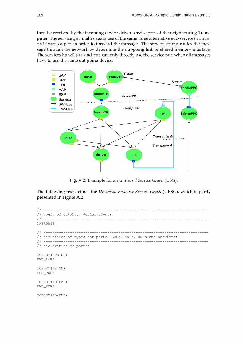
168 Appendix A. Simple Configuration Example
then be received by the incoming device driver service get of the neighbouring Trans-puter. The service get makes again use of the same three alternative sub-services route ,deliver , or put in order to forward the message. The service route routes the mes-sage through the network by determing the out-going link or shared memory interface.The services handleTP and get can only directly use the service put when all messageshave to use the same out-going device.
send receive
informTP
handleTP
route
deliver put
get informPPC
handlePPC
SAP
SRP
HRP
HAP
SSP
Service
SW-Use
HW-Use
PowerPC
Transputer
Transputer B
Transputer A
Client
Server
Fig. A.2: Example for an Universal Service Graph (USG).
The following text defines the Universal Resource Service Graph (URSG), which is partlypresented in Figure A.2:
// ---------------------------------------------------------------------------// begin of database declarations:// ---------------------------------------------------------------------------DATABASE
// ---------------------------------------------------------------------------// definition of types for ports, SAPs, SNPs, HNPs and services:// ---------------------------------------------------------------------------// declaration of ports:
IOPORT(PPC_SM)END_PORT
IOPORT(TP_SM)END_PORT
IOPORT(IO1SMP)END_PORT
IOPORT(IO2SMP)
169
END_PORT
IPORT(link_in)END_PORT
OPORT(link_in)END_PORT
OPORT(link_out)END_PORT
IPORT(link_out)END_PORT
IPORT(InLinkP)END_PORT
OPORT(OutLinkP)END_PORT
OPORT(InLinkP)END_PORT
IPORT(OutLinkP)END_PORT
// ---------------------------------------------------------------------------// declaration of SAPs:
SAP(ai_send)END_SAP
SAP(ai_receive)END_SAP
SAP(ai_informPPC)END_SAP
SAP(ai_informTP)END_SAP
SAP(ai_routeA)END_SAP
SAP(ai_routeB)END_SAP
SAP(ai_put)END_SAP
SAP(ai_deliver)END_SAP
SAP(ai_block)BLOCKS
END_SAP
SAP(ai_activate)ACTIVATES(receive)

170 Appendix A. Simple Configuration Example
END_SAP
// ---------------------------------------------------------------------------// declaration of SUPs, SCPs and SNPs:
SNP(ni_send)SELECT(ai_informTP)
END_SNP
SNP(ni_receive1)SELECT(ai_informTP)
END_SNP
SNP(ni_receive2)SELECT(ai_block)
END_SNP
SNP(ni_deliver)SELECT(ai_informPPC)
END_SNP
SNP(ni_decide)SELECT(ai_routeA)SELECT(ai_routeB)SELECT(ai_put)SELECT(ai_deliver)SELECT_MIN(1)SELECT_MAX(1)
END_SNP
SNP(ni_routeA1)SELECT(ai_put)
END_SNP
SNP(ni_routeA2)SELECT(ai_deliver)SELECT_MIN(0)SELECT_MAX(1)
END_SNP
SNP(ni_routeB)SELECT(ai_put)
END_SNP
SNP(ni_handlePPC)SELECT(ai_activate)
END_SNP
// ---------------------------------------------------------------------------// declaration of HAPs:
HAP(hi_handleTP)USES_IPORT(TP_SM)
END_HAP
HAP(hi_handlePPC)USES_IPORT(PPC_SM)
END_HAP
171
HAP(hi_get)USES_IPORT(link_in)
END_HAP
// ---------------------------------------------------------------------------// declaration of HNPs:
HNP(hi_informPPC)USES_OPORT(TP_SM)OPORTPREFERS(TP_SM, 0, ni_decide, ai_deliver)OPORTPREFERS(TP_SM, 0, ni_decide, ai_routeA)
END_HNP
HNP(hi_informTP)USES_OPORT(PPC_SM)
END_HNP
HNP(hi_put)USES_OPORT(link_out)OPORTPREFERS(link_out, 0, ni_decide, ai_put)OPORTPREFERS(link_out, 1, ni_decide, ai_routeA)OPORTPREFERS(link_out, 2, ni_decide, ai_routeB)
END_HNP
// ---------------------------------------------------------------------------// declaration of services:
SERVICE(deliver)IN(ai_deliver)OUT(ni_deliver)
END_SERVICE
SERVICE(send)IN(ai_send)OUT(ni_send)ASYN_CLIENT_OF(deliver)
END_SERVICE
SERVICE(receive)IN(ai_receive)OUT(ni_receive1)OUT(ni_receive2)SYNC_CLIENT_OF(deliver)
END_SERVICE
SERVICE(informPPC)IN(ai_informPPC)NEEDS(hi_informPPC)
END_SERVICE
SERVICE(informTP)IN(ai_informTP)NEEDS(hi_informTP)
END_SERVICE
SERVICE(get)TRIGGEREDBY(hi_get)OUT(ni_decide)
END_SERVICE

172 Appendix A. Simple Configuration Example
SERVICE(put)IN(ai_put)NEEDS(hi_put)INHIBITS_AT_MULTI_NEED(ni_decide, ai_put)
END_SERVICE
SERVICE(routeA)COSTS(3)IN(ai_routeA)OUT(ni_routeA1)OUT(ni_routeA2)
END_SERVICE
SERVICE(routeB)COSTS(2)IN(ai_routeB)OUT(ni_routeB)
END_SERVICE
SERVICE(handleTP)TRIGGEREDBY(hi_handleTP)OUT(ni_decide)
END_SERVICE
SERVICE(handlePPC)TRIGGEREDBY(hi_handlePPC)OUT(ni_handlePPC)
END_SERVICE
// ---------------------------------------------------------------------------// definition of types for CPUs, devices and media:// ---------------------------------------------------------------------------// declaration of CPUs:
CPU(Transputer)PROVIDES(handleTP)PROVIDES(put)PROVIDES(get)PROVIDES(deliver)PROVIDES(routeA)PROVIDES(routeB)PROVIDES(informPPC)HAS_IPORT(link_in)HAS_OPORT(link_out)HAS_IOPORT(TP_SM)
END_CPU
CPU(PowerPC)PROVIDES(send)PROVIDES(receive)PROVIDES(informTP)PROVIDES(handlePPC)HAS_IOPORT(PPC_SM)
END_CPU
// ---------------------------------------------------------------------------// declaration of devices:

173
DEVICE(PPCMemDev)HAS_IOPORT(PPC_SM)HAS_IOPORT(IO1SMP)
END_DEVICE
DEVICE(TPMemDev)HAS_IOPORT(TP_SM)HAS_IOPORT(IO2SMP)
END_DEVICE
DEVICE(LinkInDev)HAS_OPORT(link_in)HAS_IPORT(InLinkP)
END_DEVICE
DEVICE(LinkOutDev)HAS_IPORT(link_out)HAS_OPORT(OutLinkP)
END_DEVICE
// ---------------------------------------------------------------------------// declaration of media:
MEDIA(shared_memory)HAS_IOPORT(IO1SMP)HAS_IOPORT(IO2SMP)
END_MEDIA
MEDIA(link)HAS_OPORT(InLinkP)HAS_IPORT(OutLinkP)
END_MEDIA
// ---------------------------------------------------------------------------// end of database declarations:// ---------------------------------------------------------------------------END_DATABASE
Requirements Specification
The requirements specification defines two tasks A and B. Task A is placed on the Pow-erPC 5 and the task B is placed on the PowerPC 3. Only one communication (ComLine1)is specified. The task A wants to send a message to the task B (see Figure A.3).
# The resources define the tasks, their events,# and the communication mailboxes:
RESOURCE(Mailbox1)DELAY(5)HAS(0)EVENT(send, ai_send)EVENT(receive, ai_receive)
END_RESOURCE
RESOURCE(TaskA)IS_TASK(80, 250, 1)

174 Appendix A. Simple Configuration Example
EXECUTES(send, Mailbox1, 50) IS SEND(1)END_RESOURCE
RESOURCE(TaskB)IS_TASK(100, 250, 1)EXECUTES(receive, Mailbox1, 50) IS RECEIVE(1)
END_RESOURCE
# The place statements map the tasks onto the CPUs# and specify the source files:
PLACERESOURCE(TaskA)CPU(3)FILE(mainA.c)
END_PLACE
PLACERESOURCE(TaskB)CPU(5)FILE(mainB.c)
END_PLACE
# The communication statements connect the appropriate send# and receive events:
COMLINE(ComLine1)SENDTASK(TaskA,1)RECVTASK(TaskB,1)
END_COMLINE
END
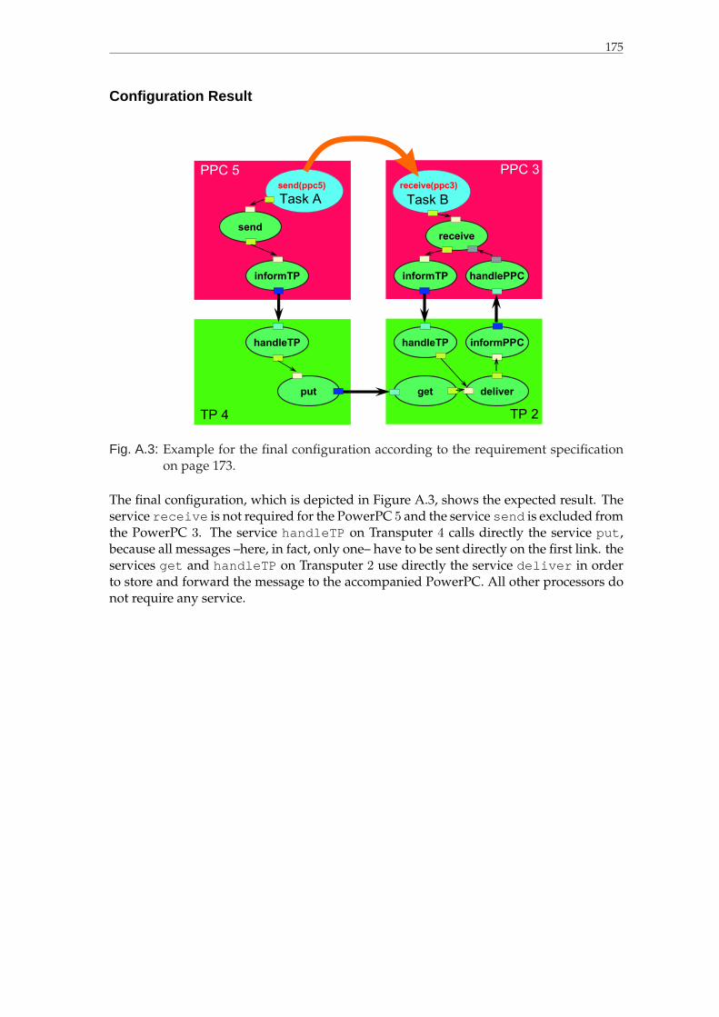
175
Configuration Result
PPC 3
TP 2
PPC 5
Task B
receive(ppc3)
Task A
send(ppc5)
TP 4
send
informTP
handleTP
put get
handleTP informPPC
deliver
informTP handlePPC
receive
Fig. A.3: Example for the final configuration according to the requirement specificationon page 173.
The final configuration, which is depicted in Figure A.3, shows the expected result. Theservice receive is not required for the PowerPC 5 and the service send is excluded fromthe PowerPC 3. The service handleTP on Transputer 4 calls directly the service put ,because all messages –here, in fact, only one– have to be sent directly on the first link. theservices get and handleTP on Transputer 2 use directly the service deliver in orderto store and forward the message to the accompanied PowerPC. All other processors donot require any service.

176 Appendix A. Simple Configuration Example

APPENDIX B
Example for the Timing Analysis
This chapter contains the source code of the requirement specification for the schedulingexample, which had been described on page 138.
Input
# ExecutionBlocks ----------------------
EXECUTION-BLOCK(t-dispatch)WAIT(OWNRES, 1)KILL_SIGNAL(OWNRES, ALL)DURATION(30)# restart Round-Robin scheduler with its timeslice (340):SIGNAL(OWNRES, 1, 340)
END_EXECUTION_BLOCK
EXECUTION_BLOCK(pre-send)DURATION(30)SIGNAL(OWNRES, 1, TRANSFER)
END_EXECUTION_BLOCK
EXECUTION_BLOCK(post-send)DURATION(30)
END_EXECUTION_BLOCK
EXECUTION_BLOCK(pre-receive)DURATION(30)
END_EXECUTION_BLOCK
EXECUTION_BLOCK(post-receive)DURATION(20)# wait on resource, iff waiting then immediately signal scheduler:SIGNALWAIT(OWNRES, 1, scheduler(OWNCPU), 1, 0)
END_EXECUTION_BLOCK

178 Appendix B. Example for the Timing Analysis
# General Tasks ------------------------
RESOURCE(scheduler)IS_TASK(0,340,0)CRITICALNESS(NO)EVENT(dispatch, t-dispatch)HAS(1) # scheduler has immediately a signal and can runUNITS(1)EXECUTES(dispatch, scheduler, 0)
END_RESOURCE
RESOURCE(idle)IS_TASK(100,100,100)CRITICALNESS(NO)
END_RESOURCE
# CPU1 ---------------------------------
RESOURCE(cpu1)IS_CPUHAS(1) # CPU has immediately a signalUNITS(1)
END_RESOURCE
# CPU2 ---------------------------------
RESOURCE(cpu2)IS_CPUHAS(1)UNITS(1)
END_RESOURCE
# comLine1 Resource --------------------
RESOURCE(comLine1)EVENT(send, pre-send, post-send)EVENT(receive, pre-receive, post-receive)DELAY(30) # the time required for the transferUNITS(5) # e.g. comLine can buffer 5 messagesHAS(0) # at begin there is no message
END_RESOURCE
# task on CPU1 -------------------------
EXECUTION_BLOCK(t1-start)# wait on resource, iff waiting immediately signal scheduler:SIGNALWAIT(OWNRES, 1, scheduler(OWNCPU), 0, 1)DURATION(30)
END_EXECUTION_BLOCK
EXECUTION_BLOCK(t1-end)DURATION(10)SIGNAL(OWNRES, 1, PERIOD)SIGNAL(scheduler, 1, PERIOD, NO_KILL)SYNC_STARTTIME(PERIOD)
END_EXECUTION_BLOCK
RESOURCE(t1)
179
IS_TASK(80, 340, 1)HAS(1) # task has immediately a signal and can runUNITS(1)EVENT(start, t1-start)EVENT(end, t1-end)EXECUTES(start, t1, 0)EXECUTES(send, comLine1, 50)EXECUTES(end, t1, 80)
END_RESOURCE
# task on CPU2 -------------------------
EXECUTION_BLOCK(t2-start)# wait on resource, iff waiting immediately signal scheduler:SIGNALWAIT(OWNRES, 1, scheduler(OWNCPU), 0, 1)DURATION(20)
END_EXECUTION_BLOCK
EXECUTION_BLOCK(t2-end)DURATION(10)SIGNAL(OWNRES, 1, PERIOD)SIGNAL(scheduler, 1, PERIOD, NO_KILL)SYNC_STARTTIME(PERIOD)
END_EXECUTION_BLOCK
RESOURCE(t2)IS_TASK(90, 340, 1)HAS(1) # task has immediately a signal and can runUNITS(1)EVENT(start, t2-start)EVENT(end, t2-end)EXECUTES(start, t2, 0)EXECUTES(receive, comLine1, 20)EXECUTES(end, t2, 90)
END_RESOURCE
# place tasks onto cpus ----------------
PLACERESOURCE(t1)CPU(cpu1)
END_PLACE
PLACERESOURCE(scheduler)CPU(cpu1)
END_PLACE
PLACERESOURCE(idle)CPU(cpu1);
END_PLACE
PLACERESOURCE(t2)CPU(cpu2)
END_PLACE
PLACE

180 Appendix B. Example for the Timing Analysis
RESOURCE(scheduler)CPU(cpu2)
END_PLACE
PLACERESOURCECPU(cpu2)
END_PLACE
PLACERESOURCE(comLine1)CPU(GLOBAL)
END_PLACE
# EOF ----------------------------------
Output
# scheduler, t1 and t2 have immediately signals!
# Schedule of cpu1:0 EBLOCK t-dispatch OF RESOURCE scheduler FROM TASK scheduler;
CONSUMES (scheduler, 1)KILLS (scheduler, 0)SIGNALS (scheduler, 1, 530)
30 TRY EBLOCK t-dispatch OF RESOURCE scheduler FROM TASK scheduler;WAIT (scheduler, 1)
30 EBLOCK t1-start OF RESOURCE t1 FROM TASK t1;CONSUMES (t1, 1)
60 TASK t1;110 EBLOCK pre-send OF RESOURCE comLine1 FROM TASK t1;
SIGNALS (comLine1, 1, 170)140 EBLOCK post-send OF RESOURCE comLine1 FROM TASK t1;170 TASK t1;200 EBLOCK t1-end OF RESOURCE t1 FROM TASK t1;
SIGNALS (t1, 1, 340)SIGNALS (scheduler, 1, 340)SYNC_STARTTIME (t1, 680)
210 TRY EBLOCK t1-start OF RESOURCE t1 FROM TASK t1;WAIT (t1, 1)SIGNALS (scheduler, 1, 210)
210 EBLOCK t-dispatch OF RESOURCE scheduler FROM TASK scheduler;CONSUMES (scheduler, 1)KILLS (scheduler, 1)SIGNALS (scheduler, 1, 740)
240 TRY EBLOCK t-dispatch OF RESOURCE scheduler FROM TASK scheduler;WAIT (scheduler, 1)
240 TASK idle;# 340 (END OF HYPERPERIOD OF THIS CPU)
# Schedule of cpu2:0 EBLOCK t-dispatch OF RESOURCE scheduler FROM TASK scheduler;
CONSUMES (scheduler, 1)KILLS (scheduler, 0)SIGNALS (scheduler, 1, 530)
30 TRY EBLOCK t-dispatch OF RESOURCE scheduler FROM TASK scheduler;WAIT (scheduler, 1)
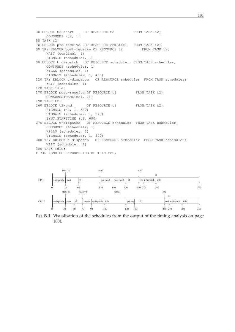
181
30 EBLOCK t2-start OF RESOURCE t2 FROM TASK t2;CONSUMES (t2, 1)
50 TASK t2;70 EBLOCK pre-receive OF RESOURCE comLine1 FROM TASK t2;90 TRY EBLOCK post-receive OF RESOURCE t2 FROM TASK t2;
WAIT (comLine1, 1)SIGNALS (scheduler, 1)
90 EBLOCK t-dispatch OF RESOURCE scheduler FROM TASK scheduler;CONSUMES (scheduler, 1)KILLS (scheduler, 1)SIGNALS (scheduler, 1, 460)
120 TRY EBLOCK t-dispatch OF RESOURCE scheduler FROM TASK scheduler;WAIT (scheduler, 1)
120 TASK idle;170 EBLOCK post-receive OF RESOURCE t2 FROM TASK t2;
CONSUMES(comLine1, 1);190 TASK t2;260 EBLOCK t2-end OF RESOURCE t2 FROM TASK t2;
SIGNALS (t2, 1, 340)SIGNALS (scheduler, 1, 340)SYNC_STARTTIME (t2, 680)
270 EBLOCK t-dispatch OF RESOURCE scheduler FROM TASK scheduler;CONSUMES (scheduler, 1)KILLS (scheduler, 1)SIGNALS (scheduler, 1, 640)
300 TRY EBLOCK t-dispatch OF RESOURCE scheduler FROM TASK scheduler;WAIT (scheduler, 1)
300 TASK idle;# 340 (END OF HYPERPERIOD OF THIS CPU)
CPU1 t1 post-send t1 t-dispatch idle
send
start
receive
t2 pre-re t-dispatch idle post-re t-dispatch idlestartt-dispatchCPU2 end
end
30 60 110 140
30 2600
end
end
start; ts
start; ts
0 170 210200 240
50 70 90 120 170 190 270 300 340
340
signal
t-dispatch
te
te
pre-send
t2
Fig. B.1: Visualisation of the schedules from the output of the timing analysis on page180f.

182 Appendix B. Example for the Timing Analysis

APPENDIX C
Language Descriptions
In the next sections we will define, which item types can be declared per database, respec-tively graph, which order should be used, and which property statements are allowedfor a specific item type. Moreover, the semantical meaning of the declarations will beexplained.
In the given examples below, the statements, which can be multiply defined, are sur-rounded by “[...]* ”. The other property statements must occur only once per databaseitem.
Comments are allowed in the form that any text after the character ’#’ followed by awhite space is ignored until the end of the line.
C.1 General Domain Knowledge
The general domain knowledge for the configuration process is defined in a database,in which all configuration items are stored. It defines a kind of knowledge base, be-cause all properties of the configuration items, like their dependencies, the alternativeselections and the constraints, are described herein. The configurator TGEN reads thisdatabase from a text file. Comments are allowed in the form that any text after the charac-ter ’#’ followed by a white space is ignored until the end of the line. The definition of thedatabase starts with the keyword DATABASEand ends with the keyword ENDDATABASE.Every line before and after this keywords are ignored. Inside the database definitionall IPORTs, OPORTs, IOPORTs, SAPs, SRPs, HAPs, HRPs, PRIMITIVEs , SERVICEs,EXECUTIONBLOCKs, CPUs, DEVICEs, and MEDIAs have to be declared. Thereby, ex-actly this order have to be used, because, for instance, before an SAP can be referenced ina service, it must have been declared.The database should start with the declaration of ports. The port declarations have thefollowing form:

184 Appendix C. Language Descriptions
IPORT(<iport-type-name>)VISIBILITY(<num>,<num>,<num>)
ENDPORT
OPORT(<oport-type-name>)VISIBILITY(<num>,<num>,<num>)
ENDPORT
IOPORT(<ioport-type-name>)VISIBILITY(<num>,<num>,<num>)
ENDPORT
The VISIBILITY statement, which is used for nearly every item of the database that ispossibly the source or destination of an edge (dependency relation), defines whether allthe assigned edges are visible at different levels inside the editor. This statement is onlymanaged by the editor tool. The ports have no other property. The port statements onlydeclare the appropriate type names as an in-port, an out-port, or an in/out-port.
After the port declarations the declaration of SAP types follow:
SAP(<sap-type-name>)VISIBILITY(<num>,<num>,<num>)PREFIX("<string>")SUFFIX("<string>")BLOCKSACTIVATES(<service-type-name>)COSTS(<int>)SELECTEDBY MAX(<num>)[ SAPFORCES(<srp-type-name>,<sap-type-name>) ]*[ SAPFAVOURS(<srp-type-name>,<sap-type-name>) ]*[ SAPINHIBITS(<srp-type-name>,<sap-type-name>) ]*
ENDSAP
The strings that are defined in the PREFIX and SUFFIX statements will be used, when thedescription of a final configuration is generated and this SAP is referred. The keywordsBLOCKSand ACTIVATES show, that the service, which has this SAP assigned, worksas a client or server service, respectively (see “Considering Communications” on page119). The keyword COSTSdefine the costs of this SAP for the configuration (see “CostFunction” on page 117). The keyword SELECTEDBY MAXdefines that this SAP can onlybe accessed from a maximum of <num> SRPs. The keywords SAPFORCES, SAPFAVOURSand SAPINHIBITS define constraints for the appropriate SRP to SAP alternatives (seeSection 6.3.4110). More than one constraint of each type can be declared.
After the SAP declarations the declaration of SRP types follow:
SRP SNP SUP SCP (<srp-type-name>)VISIBILITY(<num>,<num>,<num>)SELECTMIN(<num>)SELECTMAX(<num>)[ SELECT(<sap-type-name>) ]*
ENDSRP ENDSNP ENDSUP ENDSCP
Instead of the keyword SRPalso the keywords SNP, SUPand SCPcan be used. They willbe handled identically by the configurator TGEN. With the different keywords the expertcan distinguish different types of service dependencies. In the case of the description ofan object-oriented model (as we have in the case of DREAMS) this can be, for example,

C.1. General Domain Knowledge 185
the inheritance (SNP), the member (SCP) and the calling (or usage) dependency (SUP)between the service that contains this SRP and the service that contains the referenced SAP.But remember, the configurator TGEN handles them identically. The SELECTstatementrefers to an SAP. Thereby, an edge between the service that contains this SRP and theservice that contains the referenced SAP is defined. This edge represents the directeddependency between these services. Because the dependency is defined between the SRPand SAP of a service, the same dependency relation can be defined for another service,when it simply contains also this SRP. If more than one SELECTstatement is given, thenthis defines an OR-group of alternative dependencies. If a service wants to define anAND-group of dependencies, then it must contain one SRP per dependency. Thereby,an AND/OR-relationship can be defined. All required SRPs (AND-group) of a servicedefines possibly an OR-group. By the optional keywords SELECTMIN and SELECTMAXthe minimum and maximum number of services, which must be selected from this OR-group, can be specified. By default both values are assumed to be 1.
After the SRP declarations the declaration of HAP types follow:
HAP(<hap-type-name>)VISIBILITY(<num>,<num>,<num>)[ USES IPORT(<iport-type-name>) ]*[ USES IPORT(<ioport-type-name>) ]*[ IPORTPREFERS(<iport-type-name>,<num>,<srp-type-name>,<sap-type-name>) ]*[ IPORTINHIBITS(<iport-type-name>,<num>,<srp-type-name>,<sap-type-name>) ]*[ IPORTFORCES(<iport-type-name>,<num>,<srp-type-name>,<sap-type-name>) ]*[ IPORTPREFERS(<ioport-type-name>,<num>,<srp-type-name>,<sap-type-name>) ]*[ IPORTINHIBITS(<ioport-type-name>,<num>,<srp-type-name>,<sap-type-name>) ]*[ IPORTFORCES(<ioport-type-name>,<num>,<srp-type-name>,<sap-type-name>) ]*
ENDHAP
The HAP of a service is used in order to indicate that the service requires a hardware de-vice. The software service can bee seen as a device driver. Additionally, it is indicatedthat the direction of the data flow is from the software to the device. Devices have as-signed ports. The HAP can be connected to this ports by the use of the USESIPORTstatement. Thereby, the HAP can be connected to an in-port and to an in/out-port. TheIPORTPREFERS, IPORTFORCESand IPORTINHIBITS statements define constraints,which are guarded by this HAP.
After the HAP declarations the declaration of HRP types follow:
HRP(<hrp-type-name>)VISIBILITY(<num>,<num>,<num>)[ USES OPORT(<oport-type-name>) ]*[ USES OPORT(<ioport-type-name>) ]*[ OPORTPREFERS(<oport-type-name>,<num>,<srp-type-name>,<sap-type-name>) ]*[ OPORTINHIBITS(<oport-type-name>,<num>,<srp-type-name>,<sap-type-name>) ]*[ OPORTFORCES(<oport-type-name>,<num>,<srp-type-name>,<sap-type-name>) ]*[ OPORTPREFERS(<ioport-type-name>,<num>,<srp-type-name>,<sap-type-name>) ]*[ OPORTINHIBITS(<ioport-type-name>,<num>,<srp-type-name>,<sap-type-name>) ]*[ OPORTFORCES(<ioport-type-name>,<num>,<srp-type-name>,<sap-type-name>) ]*
ENDHRP
The HRP is defined similar to the declaration of a HAP. The HRP of a service indicates,that this service also requires for a hardware device. But the data flow is from the deviceto the service. The service can also be seen as a device driver; but more specifically it
186 Appendix C. Language Descriptions
receives the data by the device or it is activated by the device, like an interrupt serviceroutine. For this reason, the HRP can be connected to an out-port or to an in/out-port bythe USESOPORTstatement. The OPORTPREFERS, OPORTFORCESand OPORTINHIBITSstatements define again constraints, which are guarded by this HRP.
After the HRP declarations the declaration of user primitives follow:
PRIMITIVE(<primitive-type-name>)VISIBILITY(<num>,<num>,<num>)POSITION(<x>,<y>)OUT(<srp-type-name>) [ FIXED AT(<x>,<y>) ]
ENDPRIMITIVE
A user primitive can be requested by an application in the requirement specification. Thekeyword POSITION with its two parameters x and y will be ignored by the configuratorTGEN. It is managed by the editor tool and indicates the position of this node in Carte-sian coordinates inside the visualised Universal Resource Service Graph (URSG). The OUTstatement defines an edge to an SRP. Only one of this statements per user primitive is al-lowed. The OUTstatement can optionally be extended by a FIXED AT statement. This isalso ignored by TGEN. It indicates to the editor tool TEDIT, at which position this SRPhave to be placed for this user primitive.
After the user primitive declarations the declaration of services follow:
SERVICE(<service-type-name>)VISIBILITY(<num>,<num>,<num>)POSITION(<x>,<y>)COSTS(<int>)REQUIRES(<cpu-type-name>)PRIORITY(<num>)PRIORITY2(<num>)MAXPRIORITY(<num>)ORDER(<num>)PREFIX("<string>")SUFFIX("<string>")PATH(<path-name>)FILE(<file-name>)[ IN(<sap-type-name>) [ FIXED AT(<x>,<y>) ] ]*[ OUT(<srp-type-name>) [ FIXED AT(<x>,<y>) ] ]*[ NEEDS(<hap-type-name>) [ FIXED AT(<x>,<y>) ] ]*[ TRIGGEREDBY(<hrp-type-name>) [ FIXED AT(<x>,<y>) ] ]*[ ASYN CLIENT OF(<service-type-name>) ]*[ SYNC CLIENT OF(<service-type-name>) ]*[ INHIBITS(<srp-type-name>,<sap-type-name>) ]*[ FAVOURS(<srp-type-name>,<sap-type-name>) ]*[ FORCES(<srp-type-name>,<sap-type-name>) ]*[ FORCEHWUSE(<srp-type-name>,<sap-type-name>) ]*[ INHIBITS AT MULTI NEED(<srp-type-name>,<sap-type-name>) ]*[ SAY("<string>") ]*[ NEGSAY("<string>") ]*
ENDSERVICE
The service is the central type definition. It defines an item that is subject to the config-uration. The services can be included or excluded from a final configuration. The con-figurator determines, which service is part of the configuration and which is not partof the configuration. Remark, that each CPU will have its own configuration. For this

C.1. General Domain Knowledge 187
reason, the service can have assigned costs, a primary and a secondary priority, and amaximum priority, that can be reached by preferring in an OR-group (see “ConfiguringMeans Choosing of Alternatives” on page 118). The ORDER, PREFIX, SUFFIX, PATH,FILE , SAYand NEGSAYstatements define strings that can be referred during the gener-ation of this service for a final configuration. When the service is selected to be part ofthe configuration the SAYstatement will be evaluated and printed. If the service is notpart of the configuration, then the NEGSAYstatement will be evaluated and printed. Theservices are sorted after the value of the ORDERstatement and then they are printed intothe configuration description.
The IN , OUT, NEEDSand TRIGGEREDBYstatements indicate, which SAPs, SRPs, HAPsand HRPs are connected to this service. The statements ASYNCLIENT OF and SYNC-CLIENT OFdefine that this service is a client service for the server service, which is givenin the argument. There, synchronous means that the client will be blocked and asyn-chronous means that the client will not be blocked. The synchronous client will requirefor a service that will have assigned an SRP, which requests for an SAP with an BLOCKstatement. The server service will request for a service that will have assigned an SRP,which requests for an SAP with an ACTIVATE statement. By this way, the server ser-vice activates the synchronous client service. The asynchronous client sends messagesto the server service, whereas the synchronous client receives messages from the serverservice. In Appendix A a configuration example with such a client/server dependencyis described.
The FAVOURS, FORCESand INHIBITS statements define again constraints. The FORCE-HWUSEstatement identifies the specified choice element (SAP) to be chosen in an OR-group, if the service, which is assigned to that choice element, requests a specific CPUtype or a specific architecture that is provided by the CPU for which it should be se-lected. The REQUIRESstatement defines that this service possibly requires a specificCPU type to be instantiated on. This statement is referenced by the FORCEHWUSEstate-ment. The INHIBITS AT MULTI NEEDstatement prohibits the selection of the specifiedchoice element, if this service is used by more than one communication or task.
After the service declarations the declaration of execution blocks follow:
EXECUTIONBLOCK(ebName)DISABLE(resourceName)ENABLE(resourcename)PRIORITY(p)DURATION(l)[ WAIT(resourceName, n) ]* # resourceName can be keyword OWNRES[ KILL SIGNAL(resourceName, n) ]*
# resourceName can be keyword OWNRES, n can be keyword ALL[ SIGNAL(resourceName[(CpuResourceName)], n, t, [NOKILL] ) ]*
# resourceName can be keyword OWNRES, cpuResourceName can be keyword OWNCPU,# t can be keyword PERIOD or TRANSFER
[ SIGNALWAIT(resourceName, n, resourceName[(CpuResourceName)], sn, st) ]*# wResourceName can be keyword OWNRES, sCpuName can be keyword OWNCPU,# st can be keyword PERIOD or TRANSFER
SYNCSTARTTIME(t) # t can be keyword PERIODENDEXECUTIONBLOCK
The EXECUTIONBLOCKstatement defines the timing behaviour of a task and mainly of asystem call to the operating system. These statements are only considered by the timing

188 Appendix C. Language Descriptions
analysis. Its properties and semantic are described in Section 6.8133. The definition of anexecution block is also allowed to occur in the requirements specification.
Up to now all items of the Universal Service Graph (USG) are defined. Now, we willdescribe the declarations for the resource types, that can be used in the hardware andtopology description, which is the Resource Graph (RG) (see Section C.2). These resourcetypes are also part of the knowledge base and have connections to the services. Theywill have attached ports that are used in the HAPs and HRPs of the services. A resourcecan be of the type CPU, DEVICE or MEDIA, which is indicated by the use of the appro-priate keyword. These resource type declarations extend the previously defined USG tothe Universal Resource Service Graph (URSG). The resource type statements look like thefollowing:
CPU(<cpu-type-name>)VISIBILITY(<num>,<num>,<num>)POSITION(<x>,<y>)ARCHITECTURE(<architecture-type-name>)[ HAS IPORT(<iport-type-name>) [ FIXED AT(<x>,<y>) ] ]*[ HAS OPORT(<oport-type-name>) [ FIXED AT(<x>,<y>) ] ]*[ HAS IOPORT(<ioport-type-name>) [ FIXED AT(<x>,<y>) ] ]*[ PROVIDES(<service-type-name>) ]*
ENDCPU
DEVICE(<device-type-name>)VISIBILITY(<num>,<num>,<num>)POSITION(<x>,<y>)[ HAS IPORT(<iport-type-name>) [ FIXED AT(<x>,<y>) ] ]*[ HAS OPORT(<oport-type-name>) [ FIXED AT(<x>,<y>) ] ]*[ HAS IOPORT(<ioport-type-name>) [ FIXED AT(<x>,<y>) ] ]*
ENDDEVICE
MEDIA(<medium-type-name>)VISIBILITY(<num>,<num>,<num>)POSITION(<x>,<y>)[ HAS IPORT(<iport-type-name>) [ FIXED AT(<x>,<y>) ] ]*[ HAS OPORT(<oport-type-name>) [ FIXED AT(<x>,<y>) ] ]*[ HAS IOPORT(<ioport-type-name>) [ FIXED AT(<x>,<y>) ] ]*
ENDMEDIA
The PROVIDESstatement of the CPUdeclaration enumerates all services that can be in-stantiated for this CPU type. A service, which is not mentioned, will never be selectedfor a configuration for this CPU type. The ARCHITECTUREstatement of the CPUdecla-ration can enumerate some architecture names, which can be referenced by a REQUIRESconstraint of a service. Remember, that the REQUIRESconstraint can also directly refer-ence a CPU type. Additionally remark, that the REQUIRESconstraint is only evaluated,if the FORCEHWUSEconstraints is activated.
After all resources are declared the specification of the knowledge base must be termi-nated by the use of the keyword ENDDATABASE.
C.2 Hardware and Topology
In the hardware and topology description, which is the Resource Graph (RG), only twostatements are allowed. This is the HARDWAREstatement and the TOPOLOGYstatement.

C.2. Hardware and Topology 189
They also have to be placed in the given order. The HARDWAREstatement, which mustcome first, has the following form:
HARDWARE[ DEF CPU(<cpu-name>,<cpu-num>,<domain-num>,<cpu-type-name>) ]*[ SET VARCPU(<cpu-name>,<variable-name>,"<string>") ]*[ OUTPUT CPU(<cpu-name>,<file-name>) ]*[ MKFILE CPU(<cpu-name>,<file-name>) ]*[ DEF MEDIA(<medium-name>,<medium-type-name>) ]*[ DEF DEVICE(<device-name>,<device-type-name>) ]*
ENDHARDWARE
Inside the HARDWAREstatement concrete instances of CPUs, DEVICEs and MEDIAs arecreated. Therefore, Each instance have an unique identifier as its name and is of a specifictype, which must have been declared in the general domain knowledge of the UniversalResource Service Graph (URSG). A CPU have additionally assigned a unique CPU numberand a domain number, which defines the address of the CPU in the network. To eachCPU there can be assigned some variables of the type string, which will be printed intoa special output file per CPU. The name of this output file and the name of the makefilefor this CPU is defined in two extra statements.
After the HARDWAREstatement the TOPOLOGYstatement follows:
TOPOLOGYTOPOLOGYFILE(<file-name>)[ CONNECTCPUDEV(<cpu-name>,<device-name>,<port-type-name>,<num>) ]*[ CONNECTDEVMED(<device-name>,<medium-name>,<port-type-name>) ]*[ SAYONCE("<string>") ]*[ SAY("<string>") ]*
ENDTOPOLOGY
The TOPOLOGYstatement mainly defines connections between the CPUs and the devicesand between the devices and the media. For each connection a port type name must begiven. A port of exactly this name must be present in both connected resources. Thatmeans that only those ports can be connected, which have the same name! Remark, thatthe direction of the connection is defined by the ports and not by this statement. Addi-tionally, a filename can be specified. In this file the topology and other information aboutthe communications will be printed. Additionally, a topology file will be printed for eachCPU. From this files other tools can generate the routing tables for each CPU. The SAYand SAYONCEstatements contain the strings, which will be printed into these files. Thestrings of the SAY statement will be printed in all files, while the SAYONCEstatementswill be printed only in the files per CPU. Inside the strings special identifiers are recog-nised. All these special identifiers must start with the ’%’ character. These identifiers arereplaced in the output by ID numbers or lists of ID numbers of the CPUs or domains.The following identifiers are allowed:
• %CPUID()• %DOMAIN()• %LIST(DOMAINS)• %LIST(CPUS)• %LIST(CPU DOMAINS)• %LIST(LOCAL CPUS)• %LIST(LINKS TO CPU)• %LIST(LINKS ADDR)• %LIST(LINKS NCPU)• %LIST(LINKS NLINK)• %LIST(GATES OUT)
190 Appendix C. Language Descriptions
• %LIST(GATES TO CPU)• %LIST(GATES TO LINK)
C.3 Requirements Specification
The requirements specification allows only five different statements. With these state-ments the tasks, their system call events, their communications, and their placement ontothe CPUs can be described.The PACKETstatement defines the data structure of a message that will be used by a com-munication connection. It is assumed that all messages, which are sent via one specificcommunication connection between two tasks, have the same data structure.
PACKET(name)[ INT8(name) ]*[ INT16(name) ]*[ INT32(name) ]*[ INT64(name) ]*[ UINT8(name) ]*[ UINT16(name) ]*[ UINT32(name) ]*[ UINT64(name) ]*[ FLOAT32(name) ]*[ FLOAT64(name) ]*[ ARRAY8(name, size) ]*[ ARRAY16(name, size) ]*[ ARRAY32(name, size) ]*[ ARRAY64(name, size) ]*[ UARRAY8(name, size) ]*[ UARRAY16(name, size) ]*[ UARRAY32(name, size) ]*[ UARRAY64(name, size) ]*[ FARRAY32(name, size) ]*[ FARRAY64(name, size) ]*[ CSTRING(name, maxlen) ]*[ PSTRING16(name, maxlen) ]*[ PSTRING32(name, maxlen) ]*[ PACKET(name) ]*
ENDPACKET
The PACKETdeclaration is the definition of a compount type. There, basic data types,like integers or unsigned intergers and floating point types, which all can be of differentbit width, can be used. Also arrays of these basic data types can be defined. Additionally,strings can be defined, which have a maximum length and consist of a sequence of 8 Bitunsigned integers (chars). The CSTRINGis null terminated, whereas the PSTRINGs arepreceeded by an unsigned integer value, which represents their length. Inside the packetit is assumed that the string consumes maxlen size. Another packet declaration can bespecified to be a sub-type of the actual packet declaration.
The PACKETdeclaration have two major reasons: (1) the maximzum size of a messagethat is sent is specified, and (2) an algorithm can be given these information as inputin order to change automatically the endianess of the message. Thereby, the tasks ofa communication can be placed on processors with different endianess (low/high-byteorder).
C.3. Requirements Specification 191
The most important definition in the requirement specification is the declaration of aresource:
RESOURCE(resourceName)IS TASK(runtime, period, priority) IS CPUCRITICALNESS(NO SOFT FIRM HARD)DELAY(delay)UNITS(items)HAS(items)[ EVENT(eventName, [ ebName ]+ ) [ IS SEND(num) RECEIVE(num) ] ]*[ EXECUTES(eventName, resourceName, time [ , delay [ , items ]] )
[ IS SEND(num) RECEIVE(num) ] ]*# delay and items can be keyword DEFAULT
ENDRESOURCE
A resource is subject to the signal() and wait() procedures of the behaviour descrip-tion of an execution block for the timing analysis. With the property statements IS TASKor IS CPUthe resource can be qualified to be a task or a CPU. Only one of these state-ments must be used and they are optional. Each resource has a counter for items andit works like a counting semaphore. The items which are initially present, are specifiedwith the HASproperty statement. Each signal() and wait() , which is executed onthis resource, will increment or decrement these counter accordingly. The DELAYprop-erty specifies that the increment will be delayed for a specific time. Thus, between theproduction and a possible consume of the items must be at least delay time units. If thedelay is not given for a resource, then it will be assumed to be zero. Each resource mustdefine some events, that are regarded as system calls. Each of these events is attacheda list of execution blocks. A task or any other execution block can execute these events.An execution block can emit a signal() to any other resource or can execute a wait()for a specified number of items on any resource. With these declarations the behaviourin form of sequentially executing atomic blocks with an signal/wait mechanism can bespecified (see Section 6.8133).
When the resource is specified to be a task, then the EXECUTESproperties are allowed tobe specified. These properties of a task define when a task calss which system call. In fact,the system call must be the name of an event, which is executed on a specific resource.Additionally, the name of the event is assumed to be a primitive of the Universal ServiceGraph (USG), which is required by the task.
The communication between two tasks has to be modelled in the following way: Thesender task has to call a SENDevent. The receiver task has to call a RECEIVEevent. BothEvents are marked by specific keywords and are identified by a number. For the routinga connection, respectively an in/out-dependency between two tasks will be defined by aCOMLINEdeclaration:
COMLINE(comName)SENDTASK(name1,num 1)RECVTASK(name2,num 2)PACKET(name3)
ENDCOMLINE
This declaration defines that task name1 sends the message name3 to the receiving taskname2. Hereby, the numth
1 send event of the sender task and the numth2 receive event
of the receiver task will be used. The period of this connection or the minimal messageinterarrival time is specified by the minimum of the sender’s and receiver’s period.

192 Appendix C. Language Descriptions
Last but not least, for the routing the placement of the tasks onto the CPUs must bespecified. This is done by a PLACEdeclaration:
PLACERESOURCE(resourceName)CPU(CpuResourceName)[ FILE(filename) ]*
ENDPLACE
Each task must be placed on a CPU. Optionally, some file names can be specified, whichidentify the source files that define the task’s source code. These will be used for thegeneration of the Makefiles for each CPU.

Index
A
ABS, see Anti-lock Braking Systemabsolute finishing jitter, 67absolute release jitter, 67acceptance test, 65adaptable, 26AI, see artificial intelligenceAMPHION, 25AND/OR-tree, 29, 33, 39
canonical form, 29Anti-lock Braking System, 7API, 99, see Application Programming
Interface, 153Application Programming Interface, 99,
110, 153artificial intelligence, 38ASCET-SD, 25Assumption-Based Truth Maintenance Sys-
tem, 39Asynchronous Transfer Mode, 85ATM, see Asynchronous Transfer ModeATMS, see Assumption-Based Truth Main-
tenance System
B
backtracking, 31dependency-directed, 31knowledge-based, 31monotone, 31
BF, see graph search: algorithms: best-first search
BFS, see graph search: algorithms: breadth-first-search
broadcast, 77
bus, 77busy period, 73
C
CAN, see Controller Area Network, 142capacity, 75case-based reasoning, 40CBR, see case-based reasoningCentral Processing Unit, 108Central Processing Unit, processor, 134CFS, see graph search: algorithms: cheapest-
first-searchchannel, 77channel-oriented communication, 93CHIMERA, 57CLOSED-list, 30CM, see Configuration Managementcommunication
channel-oriented, 77multi-cast, 77packet-oriented, 77request, 78
communication delay, 65communication network, 77compositional hierarchies, 39configurable, 26configuration, 20, 26
aim, 19by a simulation system, 40case-based, 40constraint-based, 40definition, see aimhybrid systems, 41problem characteristics, 37
193

194 Index
process, 20automatic, 20interactive, 20
resource-based, 39rule-based, 38skeleton-based, 41structure-based, 39systems
AKON, 41ALL-RISE, 42artdeco, 44CAS, 44, 46COSMOS, 44, 46ET-EPOS, 44, 46KONWERK, 44MMC-KON, 42PLAKON, 42R1/XCON, 41SCE, 45, 46SECON, 45, 46SICONFEX, 42
with concept hierarchies, 39with truth maintenance systems, 38
Configuration Management, 23configurator, 20configuring, 28connection
multi-hop, 77point-to-point, 77
constraintnetwork, 40propagation, 40types, 40
Constraint Satisfaction Problem, 40constraints
precedence, 65resource, 65timing, 64
controller, 62Controller Area Network, 108, 142correctness
validation, 38cost labelling, 35cost function, 35
order-preserving, 36recursive, 35summing, 36
CPU, see Central Processing Unit
criticalness, 67CSP, see Constraint Satisfaction Problemcustomisable, 26customisation, 26
D
DAG, see Directed Acyclic Graphdatagram, 77DAVINCI, 58deadline, 62, 64Deadline Monotonic, 72design space, 27Deutsche Forschungsgemeinschaft, 162Deutsche Forschungsgemeinschaft, IVdevice driver, 109DFG, see Deutsche Forschungsgemeinschaft,
162DFS, see graph search: algorithms: depth-
first-searchDirected Acyclic Graph, 98Distributed Extensible Application Man-
agement System, 51DM, see Deadline Monotonicdouble buffering, 82DREAMS, see Distributed Real-Time Ex-
tensible Application ManagementSystem
E
Earliest Deadline First, 69, 72Earliest Due Date, 69ECU, see Embedded Control UnitEDD, see Earliest Due DateEDF, see Earliest Deadline First, see Earli-
est Deadline FirstEDF∗, 70, 73Electronic Stabilisation Programme, 7Embedded Control Unit, 7embedded system, 62ESP, see Electronic Stabilisation Programmeexpert knowledge, 27expert system, 38eXtensible Markup Language, 125
F

Index 195
Fault tolerance, 63feasible, 68feasible schedule, 65footers, 77fragmentation, 77
G
GBF, see graph search: algorithms: gen-eral best-first search
general domain knowledge, 28graph composition, 114graph search
algorithmsA∗, 36, 36AO, 36, 36AO∗, 36best-first search, 32, 32, 34, 35BF, see best-first search, see best-
first searchBFS, see breadth-first-searchbreadth-first-search, 31, 36CFS, see cheapest-first-searchcheapest-first-search, 32, 36depth-first-search, 31, 36DFS, see depth-first-searchGBF, see general best-first search,
see general best-first searchGBF∗, 34general best-first search, 32, 34, 36hillclimbing, 32Z, 35Z∗, 35, 36
graph traversal algorithms, 31blind, see uninformeddirected, see informedguided, see informedinformed, 31, 32uninformed, 31
H
HAP, see TEReCS: definitions: HardwareAccess Point
HC, see graph search: algorithms: hill-climbing
headers, 77High Performance Computing, 63
HPC, see High Performance ComputingHRP, see TEReCS: definitions: Hardware
Request Pointhyper edge, 30hyper-graph, 30hyperperiod, 67
I
Intellectual Property, 161interrupt handler, 109IP, see Intellectual Property
J
JTMS, see Justification-Based Truth Main-tenance System
Justification-Based Truth Maintenance Sys-tem, 39
K
knowledgetransfer, 21
L
Latest Deadline First, 70LDF, see Latest Deadline FirstLogical-Based Truth Maintenance System,
39LTMS, see Logical-Based Truth Mainte-
nance System
M
Maintainability, 63merit labelling, 35message, 77MULTI-THREADED GRAPH CLUSTERING,
25mutual exclusion, 65
O
OPEN-list, 30, 31, 32operating system

196 Index
AMBROSIA, 51AMBROSIA/ MP, 55APERTOS, 50CHAOS, 50CHOICES, 50ECOS, 49ERCOS, 25EXOKERNEL, 50LINUX, 50MARS, 84PEACE, 51PURE, 49, 51QNX, 48RTEMS, 48SYNTHESIS, 49, 50VIRTUOSO, 49VXWORKS, 25, 50
P
packet, 77packet-oriented communication, 93path, 77PCG, see TEReCS: definitions: Process
and Communication GraphPCP, see Priority Ceiling Protocolperiod, 66phase, 67PIP, see Priority Inheritance ProtocolPredictability, 63preemption, 67, 69Priority Ceiling Protocol, 87Priority Inheritance Protocol, 85Priority Inversion Phenomenon, 85problem graph, 29problem reduction graph, 30problem-solving domain knowledge, 28problem-specific domain knowledge, 28process communication, 77processor, 134processor utilisation factor, 71protocol information, 77
Q
QoS, see quality of service, see Quality ofService
Quality of Service, 63
quality of service, 20
R
Rate Monotonic, 72reactive system, 62real-time
analysis, 65real-time computer system, 64real-time computing, 62real-time system
predictable, 65REGIS, 59Remote Object Invocation, 51requirements specification, 20response time, 62RG, see TEReCS: definitions: Resource
Graphring, 77RM, see Rate MonotonicROI, see Remote Object Invocationroute, 77routing, 78routing table, 78RSG, see TEReCS: definitions: Resource
Service Graph
S
SAP, see TEReCS: definitions: Service Ac-cess Point
schedulability test, 64, 65schedule, 67Scheduling
Background, 75SCI, see Serial Communication InterfaceSCM, see Software Configuration Man-
agementSerial Communication Interface, 154Server
Deferrable, 75Fixed Priority, 75Polling, 75Priority Exchange, 76
SFB 501, 25Software Configuration Management, 23solution graph, 29, 30solution-base graph, 30

Index 197
Spring, 70SPRING, 70SRP, see TEReCS: definitions: Service Re-
quest PointStateCharts, 25STATEMATE, 25stimuli, 62stop-and-go queuing, 82system
event-driven, 84time-driven, 84
T
TANA, 5, 17, 135, 159, 160, 163taxonomical hierarchies, 39TCLUSTER, 5, 159TDESIGN, 5, 159, 160TDMA, see Time Devision Multiple Ac-
cessTEDIT, 5, 113, 159, 160, 186TEReCS, III, IV, 4, see Tools for Embed-
ded Real-time Communication Sys-tems, 9–16, 22, 24, 29, 41, 42, 45,49, 52, 59, 64, 87, 102, 104, 105,see Tools for Embedded Real-TimeCommunication Systems, 106, 110–114, 118, 119, 126–132, 134, 135,138–140, 147–151, 153–155, 159–163, 167
definitionsProcess and Communication Graph,
111, 114, 115Resource Graph, 107, 112–115, 159Resource Service Graph, 114, 115Universal Resource Graph, 108, 108,
110, 112–114, 124Universal Resource Service Graph,
110, 110, 111, 113–119, 124, 156,159, 160, 162
Universal Service Graph, 109, 109,110, 112, 114, 115, 119, 120, 122,124, 125, 132, 133, 147, 188
Hardware Access Point, 109, 109,110, 119, 185, 187, 188
Hardware Request Point, 109, 109,110, 119, 185–188
port, 108
Process and Communication Graph,107, 116, 125
Resource Graph, 116, 124, 126, 165,166, 188
service, 106, 107, 108, 109, 110, 113–115, 125, 126, 153, 183, 185–188
Service Access Point, 108, 108, 109–111, 117, 118, 126, 129, 153, 183–185, 187
Service Request Point, 108, 108, 109–111, 117, 118, 121, 129, 130, 153,184–187
super-service, 120, 120, 121Universal Resource Service Graph,
115, 116, 124, 126, 168, 186, 188,189
Universal Service Graph, 119, 157,168, 188, 191
User Access Point, 110user primitive, 102, 106, 110, 112,
114, 115, 120, 121, 126, 167, 186TGEN, 5, 17, 22, 41, 42, 45, 124–127, 155,
159, 160, 183–186Time Devision Multiple Access, 84Time-triggered Protocol, 84Timeliness, 63TMS, see truth maintenance systemTools for Embedded Real-Time Commu-
nication Systems, 105Tools for Embedded Real-time Commu-
nication Systems, 5Tree search, 69truth maintenance system, 39TTP, see Time-triggered Protocol
U
UAP, see TEReCS: definitions: User Ac-cess Point
under-specification, 26URG, see TEReCS: definitions: Universal
Resource GraphURSG, see TEReCS: definitions: Univer-
sal Resource Service GraphUSG, see TEReCS: definitions: Universal
Service Graph
W

198 Index
weight function, 35worst-case execution time, 64worst-case response time, 82
X
XML, see eXtensible Markup Language

Bibliography
[1] P. Altenbernd. CHaRy: The C-LAB Hard Real-Time System to Support Mechatron-ical Design. In Int. Conf. and Workshop on Engineering of Computer Based Systems(ECBS), 1997. (page 12, 133)
[2] P. Altenbernd, C. Boke, G. D. Castillo, C. Ditze, E. Erpenbach, U. Glasser, W. Hardt,B. Kleinjohann, G. Lehrenfeld, F. J. Rammig, C. Rust, F. Stappert, J. Stroop, andJ. Tacken. Paradise: Design Environment for Parallel & Distributed, EmbeddedReal-Time Systems. In F. J. Rammig, editor, Distributed and Parallel Embedded Sys-tems, Proc. of the 1st International IFIP WG 10.3/WG 10.5 Workshop on Distributedand Parallel Embedded Systems (DIPES), Paderborn University, Germany, October5-6, 1998, pages 181–190. Kluwer Academic Publishers, Norwell, Massachusetts,number 25 of IFIP edition, 1999. (page 161, 162)
[3] B. Appleton. Assembling Configuration Management Environments Project.WWW pages at http://www.enteract.com/∼bradapp/acme/, 1998. (page 24)
[4] N. C. Audsley, A. Burns, M. F. Richardson, K. Tindell, and A. J. Wellings. ApplyingNew Scheduling Theory to Static Priority Preemptive Scheduling. Software Engi-neering Journal, 8(5):284–292, September 1993. (page 73)
[5] N. C. Audsley, A. Burns, M. F. Richardson, and A. J. Wellings. Hard Real-TimeScheduling: The Deadline Monotonic Approach. In Workshop on Real-Time Operat-ing Systems. IEEE, 1992. (page 73)
[6] W. Baginsky, H. Endres, G. Geissing, and L. Philipp. Basic Architectural Featuresof Configuration Expert Systems for Automation Engineering. In Proc. of IEEE Con-ference ”International Workshop on Artificial Intelligence for Industrial Applications”,Hittachi City, 1988. Also TEX-K Report No. 11, Energy and Automation Group,Siemens AG, ESTE 12, Erlangen, Germany. (page 42)
[7] V. E. Barker, D. E. O’Connor, J. Bachant, and E. Soloway. Expert systems for config-uration at Digital: XCON and beyond. Communications of the ACM, 32(3):298–318,March 1989. ACM Press, New York, NY, USA, ISSN:0001-0782. (page 41)

200 Bibliography
[8] S. K. Baruah, L. E. Rosier, and R. R. Howell. Algorithms and Complexity Con-cerning the Preemptive Scheduling of Periodic, Real-Time Tasks on One Processor.Journal of Real-Time Systems, 2, 1990. (page 73)
[9] L. Baum, M. Becker, L. Geyer, G. Molter, and P. Sturm. Driving the Composition ofRuntime Platforms By Architectural Knowledge. In Proc. of the 8th ACM SIGOPSEuropean Workshop: Support for Composing Distributed Applications, Sintra, Portugal,September 1998. (page 25)
[10] L. Baum, L. Geyer, G. Molter, S. Rothkugel, and P. Sturm. Architecture-CentricSoftware Development Based on Extended Design Spaces. In Proc. of the ARES Sec-ond Int’l Workshop on Development and Evolution of Software Architectures for ProductFamilies, Las Palmas de Gran Canaria, Spain, Feb. 1998. (page 25)
[11] R. Berg, J. Cordsen, J. Nolte, B. Oestmann, M. Sander, H. Schmidt, F. Schon, andW. Schroder-Preikschat. The PEACE Family of Distributed Operating Systems.Technical report, GMD-FIRST, 1991. 44 pages. (page 51)
[12] G. Berry and G. Gonthier. The Esterel synchronous programming language: De-sign, semantics, implementation. Science of Computer Programming, 19(2):87–152,1992. (page 3)
[13] H. K. Buning, D. Curatolo, M. Hoffmann, R. Lemmen, M. Suermann, and B. Stein.ARTDECO - Entwurfsunterstutzung in der Hydraulik. KI – Kunstliche Intelligenz:Forschung, Entwicklung, Erfahrungen, 9(5):49–55, September 1995. (page 44)
[14] C. Boke. Software Synthesis of Real-Time Communication System Code for Dis-tributed Embedded Applications. In Proc. of the 6th Annual Australasian Conf. onParallel and Real-Time Systems (PART), Melbourne, Australia, December 1999. IFIP,IEEE. (page 52, 162)
[15] C. Boke. Combining Two Customization Approaches: Extending the Customiza-tion Tool TEReCS for Software Synthesis of Real-Time Execution Platforms. In Proc.of the Workshop on Architectures of Embedded Systems (AES), Karlsruhe, Germany, Jan-uary 2000. (page 14, 52, 162)
[16] C. Boke, C. Ditze, H. J. Eickerling, U. Glasser, B. Kleinjohann, F. J. Rammig, andW. Thronike. Software IP in Embedded Systems. In Proc. of the Forum on DesignLanguages (FDL), Lyon, France, September 1999. (page 52, 162)
[17] C. Boke, M. Gotz, T. Heimfarth, D. El-Kebbe, F. J. Rammig, and S. Rips. (Re-)Configurable Real-time Operating Systems and their Applications. In Proc. ofWORDS 2003. IEEE, January 2003. (page 162)
[18] C. Boke, M. Hubel, F. J. Rammig, and C. Rust. Zero-Overhead Pr/T-Net Execution.In Proc. of the SCS International European Simulation Multi-Conference (ESM), Gent,Belgium, May 23-26 2000. (page 161, 162)
[19] C. Boke and F. J. Rammig. Entwurf konfigurierbarer, echtzeitfahiger Kommunika-tionssysteme. In journal “Informationstechnik und Technische Informatik” (it+ti), vol-ume 2. R. Oldenbourg Verlag, Germany, 1999. (in German). (page 25, 52, 162)

Bibliography 201
[20] P. Bratley, M. Florian, and P. Robillard. Scheduling with Earliest Start and Due DateConstraints. Naval Research Logistics Quarterly, 18(4), 1971. (page 70)
[21] P. Brinch Hansen. Operating System Principles. Prentice-Hall, 1973. (page 85)
[22] H. K. Buning and B. Stein. Supporting the Configuration of Technical Systems. InM. Hiller and B. Fink, editors, Second Conference on Mechatronics and Robotics, pages417–432. IMECH, Mechatronics Institute, Moers, Germany, July 1993. (page 44)
[23] A. Burns. Preemptive Priority based Scheduling: An Appropriate engineering ap-proach. Technical report, Real-time Systems Research Group, Dept. of Comp. Sc.,University of York, UK, 1993. (page 105)
[24] C. Burrows. Configuration Management: Coming of Age in the Year 2000. InCrossTalk magazine, pages 12–16. U.S. Air Force’s Software Technology SupportCenter (STSC), March 1999. http://www.stsc.hill.af.mil/CrossTalk/. (page 23)
[25] G. C. Buttazzo. Hard Real-Time Computing Systems: Predictable Scheduling Algorithmsand Applications. The Kluwer international series in engineering and computer sci-ence. Kluwer Academic Publishers, Boston Dordrecht London, real-time systemsedition, 1997. (page 62, 63, 68, 69, 71, 72, 73, 74, 75, 76, 86, 87)
[26] R. Campbell, G. Johnston, and V. Russo. Choices — Class Hierarchical Open In-terface for Custom Embedded Systems. ACM Operating Systems Review, 21(3):9–17,July 1987. (page 50)
[27] H. Chetto, M. Silly, and T. Bouchentouf. Dynamic Scheduling of Real-Time Tasksunder Precedence Constraints. Journal of Real-Time Systems, 2, 1990. (page 70)
[28] R. P. Chivukula, C. Boke, and F. J. Rammig. Customizing the Configuration Processof an Operating System Using Hierarchy and Clustering. In Proc. of the 5th IEEEInternational Symposium on Object-oriented Real-time distributed Computing (ISORC),pages 280–287, Crystal City, VA, USA, 29 April – 1 May 2002. IFIP WG 10.5. ISBN0-7695-1558-4. (page 162)
[29] R. Conradi and B. Westfechtel. Configuring Versioned Software Products. InSoftware Configuration Management, ICSE’96 SCM-6 Workshop, volume LNCS 1167,pages 88–109. Springer, 1996. (page 24)
[30] R. Conradi and B. Westfechtel. Version models for software configuration man-agement. Technical Report AIB 96-10, RWTH Aachen, Germany, October 1996.ftp://ftp-i3.informatik.rwth-aachen.de/pub/reports/CW96a.ps.gz. (page 24)
[31] M. Cornero, F. Thoen, G. Goossens, and F. Curatelli. Software Syn-thesis for Real-Time Information Processing Systems. In P. Marwedeland G. Goossens, editors, Code Generation for Embedded Processors, Proc.of the 1st Workshop on Code Generation for Embedded Processors,Dagstuhl (Germany). Kluwer Academic Publishers, Boston, February 1995.http://146.103.254.1/vsdm/projects/sw synthesis/publication.html. (page 25)
[32] R. Cunis, H. Bode, A. Gunter, H. Peters, and I. Syska. Wissensreprasentation inPLAKON. Tex-k report no. 10, Fachbereich Informatik, Universitat Hamburg, Ger-many, 1988. (page 43)

202 Bibliography
[33] R. Cunis, A. Gunter, I. Syska, H. Bode, and H. Peters. PLAKON – Ein System zurkonstruktion in technischen Domanen. In Proc. of KOMMTECH-88, Germany, 1988.Also TEX-K Report No. 13, Fachbereich Informatik, Universitat Hamburg. (page43)
[34] R. Cunis, A. Gunter, and H. Strecker, editors. Das PLAKON-Buch. Informatik Fach-bericht 266. Springer-Verlag, 1991. (page 42)
[35] Cygnus. eCos – Embedded Cygnus operating system1. Technical white paper,Cygnus, 1999. (page 49)
[36] A. Damm, J. Reisinger, W. Schwabl, and H. Kopetz. The real-time operating systemof MARS. ACM Operating Systems Review, 23(3):141–157, July 1989. (page 84)
[37] M. L. Dertouzos. Control Robotics: The Procedural Control of Physical Processes.Information Processing, 74, 1974. (page 69)
[38] E. W. Dijkstra. Cooperating Sequential Processes. In F. Genuys, editor,. AcademicPress, New York, 1968. (page 85)
[39] C. Ditze. DREAMS – Concepts of a Distributed Real-Time Management System.In Proc. of the 1995 IFIP/IFAC Workshop on Real-Time Programming (WRTP), 1995.(Another copy with quite identical contents appeared in journal Control EngineeringPractice, Vol. 4 No. 10, 1996.). (page 51)
[40] C. Ditze. A Customizable Library to support Software Synthesis for Embedded Ap-plications and Micro-Kernel Systems. In Proc. of the Eighth ACM SIGOPS EuropeanWorkshop, Sintra, Portugal, September 1998. (page 51)
[41] C. Ditze. A Step towards Operating System Synthesis. In Proc. of the 5th AnnualAustralasian Conf. on Parallel And Real-Time Systems (PART). IFIP, IEEE, 1998. (page49, 51)
[42] C. Ditze. Towards Operating System Synthesis. Phd thesis, Department of ComputerScience, Paderborn University, Paderborn, Germany, 1999. (page 24, 49, 51, 63, 127)
[43] C. Ditze and C. Boke. Supporting Software Synthesis of Communication Infrastruc-tures for Embedded Real-Time Applications. In Proc. of the 15th IFAC Workshop onDistributed Computer Control Systems (DCCS), Como, Italy, September 1998. (page25, 51, 153, 162)
[44] D. R. Engler, M. F. Kaashoek, and J. O’Toole. Exokernel: An Operating SystemArchitecture for Application-Level Resource Management. In Proc. of the 15th Sym-posium on Operating System Principles. ACM Press, December 1995. (page 50)
[45] ASCET-SD and ERCOS by ETAS GmbH & Co. KG. at http://www.etas.de/. (page3, 25)
[46] K. Forbus and J. deKleer. Building Problem Solvers. MIT Press, 1993. (page 39)
[47] P. Friedland. Knowledge-Based Experiment Design in Molecular Genetics. ReportSTAN-CS-79-771, Stanford University, 1979. (page 39)
1 http://www.cygnus.com/ecos

Bibliography 203
[48] J. S. Gero. Design Prototypes: A Knowledge Representation Scheme for Design. AIMagazine, 11:26–36, 1990. (page 27)
[49] A. Gheith and K. Schwan. CHAOSarc: Kernel support for multiweight objects,invocations, and atomicity in real-time multiprocessor applications. ACM Transac-tions on Computer Systems, 11(1)(1):33–72, February 1993. (page 50)
[50] A. Gunter and C. Kuhn. Knowledge-Based Configuration - Survey and FutureTrends. In F. Puppe, editor, Expertensysteme ’99 Lecture Notes. Springer, 1999.http://www.hitec-hh.de/aguenter/literatur.html. (page 37)
[51] A. Gunter, I. Kreuz, and C. Kuhn. Kommerzielle Software-Werkzeuge fur die Kon-figurierung von technischen Systemen. Kunstliche Intelligenz, 3:61–65, 1999. ArenD-Tap Verlag, http://www.hitec-hh.de/aguenter/literatur.html. (page 44, 46)
[52] A. Gunter, I. Syska, and R. Cunis. PLAKON Anforderungskatalog. TEX-K Report 4,Fachbereich Informatik, Universitat Hamburg, Germany, 1987. (page 42, 43)
[53] S. Golestani. A Stop-And-Go Queueing Framework for Congestion Management.In Proceedings of SIG-COMM’90, June 1990. (page 82)
[54] R. L. Graham, E. L. Lawler, J. K. Lenstra, and A. H. G. Rinnooy Kan. Optimiza-tion and Approximation in Deterministic Sequencing and Scheduling: A Survey.Annals of Discrete Mathematics, 5, 1979. (page 68)
[55] H. Gusgen, U. Junker, and A. Voss. Constraints in a Hybrid Knowledge Represen-tation System. In IJCAI-87, pages 30–33, Los Altos, 1987. Morgan Kaufmann. (page42)
[56] A. Gunter. KONWERK - ein modulares Konfigurierungswerkzeug. In M. Richterand F. Maurer, editors, Expertensysteme 95 (XPS-95), pages 1–18. Hundt, Koln, 1995.(page 44)
[57] A. Gunter (ed.). Wissensbasiertes Konfigurieren - Ergebnisse aus dem Projekt PROKON.infix Verlag, St. Augustin, 1995. (page 44)
[58] N. Halbwachs. Synchronous Programming of Reactive Systems. Kluwer AcademicPublishers, Boston Dordrecht London, 1993. (page 3)
[59] W. Hardt, F. J. Rammig, C. Boke, C. Ditze, J. Stroop, A. Rettberg, G. D. Castillo,and B. Kleinjohann. IP-based System Design within the PARADISE Design En-vironment. In Euromicro Journal “Systems Architecture”. Elsevier, 2000. (page 161,162)
[60] D. Harel. Statecharts: A Visual Formalism for Complex Systems. Science of Com-puter Programming, 8:231–274, 1987. (page 25)
[61] H. Haugeneder, E. Lehmann, and P. Struss. Knowledge-Based Configuration ofOperating Systems – Problems in Modeling the Domain Knowledge. In Proc. Wis-sensbasierte Systeme, pages 121–134, Berlin, Germany, 1985. Springer. (page 42)
[62] M. Heinrich. Ressourcenorientiertes Konfigurieren. Kunstliche Intelligenz, 7(1):11–15, 1993. (page 44)

204 Bibliography
[63] W. Horn. Some Simple Scheduling Algorithms. Naval Research Logistics Quarterly,21, 1974. (page 69)
[64] StateMate by I-Logix. at http://www.ilogix.com/. (page 3, 25)
[65] INMOS Limited. ANSI C toolset user manual, August 1990. (page 14)
[66] International Organization for Standardization (ISO). International Standard35.100.01 Open Systems Interconnection (OSI). ISO/IEC 7498-1, 1994. Basic Refer-ence Model at http://www.iso.ch/. (page 52, 96, 110)
[67] ISO. Road Vehicles – Interchange of Digital Information – Controller Area Network(CAN) for High Speed Communication. ISO/DIS Standard 11898, 1992. (page 83,142)
[68] J. R. Jackson. Scheduling a Production Line to Minimize Maximum Tardiness. InManagement Science Research Project, volume 43, Los Angeles, 1955. University ofCalifornia. (page 69)
[69] K. Jeffay and D. L. Stone. Accounting for Interrupt Handling Costs in DynamicPriority Task Systems. In Real-Time Systems Symposium, pages 212–221. IEEE, De-cember 1993. (page 73)
[70] K.-P. Jaker, P. Klingebiel, U. Lefarth, J. Richert, and R. Rutz. Tool integration byway of a computer-aided mechatronic laboratory (CAMeL). In 5th IFAC/IMACSSymposium on Computer Aided Design in Control Systems, 1991. (page 3)
[71] H. Kise, T. Ibaraki, and H. Mine. A Solvable Case of the One Machine SchedulingProblem with Ready and Due Times. Operations Research, 26:121–126, 1978. (page69)
[72] H. Kopetz. Real-Time Systems: Design Principles for Distributed Embedded Applica-tions. Kluwer Academic Publishers, Boston Dordrecht London, 1997. (page 64,84)
[73] H. Kopetz, A. Damm, C. Koza, and M. Mulozzani. Distributed fault tolerant real-time systems: The Mars approach. IEEE Micro, pages 25–40, 1989. (page 84)
[74] H. Kopetz, G. Fohler, G. Grunsteidl, H. Kantz, G. Pospischil, P. Puschner,J. Reisinger, R. Schlatterbeck, W. Schutz, A. Vrchoticky, and R. Zainlinger. Real-time system development: The programming model of MARS. In Proc. of the Int.Symp. on Autonomous Decentralized Systems, pages 190–199, March 1993. (page 84)
[75] D. Ku and G. de Micheli. Relative Scheduling Under Timing Constraints. In Proc.of the 27th ACM/IEEE Design Autom. Conference, Orlando, Florida, USA, June 1990.(page 25)
[76] E. L. Lawler. Optimal Sequencing of a Single Machine Subject to Precedence Con-straints. Managements Science, 19, 1973. (page 70)
[77] J.-I. Le Boudec. The Asynchronous Transfer Mode: a tutorial. Computer Networksand ISDN Systems, 24:279ff., 1992. (page 85)

Bibliography 205
[78] E. Lehmann, R. Enders, H. Haugeneder, R. Hunze, C. Johnson, L. Schmid, andP. Struss. SICONFEX – ein Expertensystem fur die betriebliche Konfigurierungeines Betriebssystems. In Proc. GI/OCG/OGI-Jahrestagung, pages 792–805, Berlin,Germany, 1985. Springer. (page 42)
[79] J. Lehoczky, L. Sha, and J. K. Strosnider. Enhanced Aperiodic Responsiveness inHard Real-Time Environments. In Proceedings of the IEEE Real-Time Systems Sympo-sium, December 1987. (page 75, 76)
[80] J. P. Lehoczky. Fixed Priority Scheduling of Periodic Tasks with Arbitrary Dead-lines. In Proc. of the 11th IEEE Real-Time Systems Symposium, pages 201–209, 1990.(page 83)
[81] J. P. Lehoczky and S. Ramos-Thuel. An Optimal Algorithm for Scheduling Soft-Aperiodic Tasks in Fixed-Priority Preemptive Systems. In Proceedings of the IEEEReal-Time Systems Symposium, December 1992. (page 76)
[82] J. K. Lenstra and A. H. G. Rinnooy Kan. Optimization and Approximation in De-terministic Sequencing and Scheduling. Annals of Discrete Mathematics, 5:287–326,1977. (page 69)
[83] J. K. Lenstra, A. H. G. Rinnooy Kan, and P. Bruckner. Complexity of MachineScheduling Problems. Annals of Discrete Mathematics, 1:343–362, 1977. (page 69)
[84] J. Y. T. Leung and J. Whitehead. On the Complexity of Fixed-Priority Scheduling ofPeriodic Real-Time Tasks. Performance Evaluation, 4(2):237–250, 1982. (page 72)
[85] C. L. Liu and J. W. Layland. Scheduling Algorithms for Multiprogramming in aHard-Real-Time Environment. Journal of the ACM, Vol. 20(1):46–61, January 1973.(page 71, 72)
[86] M. Lowry, A. Philpot, T. Pressburger, and I. Underwood. A Formal Approach toDomain-Oriented Software Design Environments. In Proc. of IEEE Knowledge-BasedSoftware Engineering Conf., pages 48–57, Los Alamitos, CA, 1994. (page 25)
[87] H. Massalin. Synthesis: An Efficient Implementation of Fundamental Operating SystemServices. Phd thesis, Columbia University, 1992. (page 49)
[88] H. Massalin and C. Pu. Threads and input/output in the Synthesis kernel. In 12thSymposium on Operating System Principals, ACM SIGOPS, volume 23, pages 191–201.ACM, December 1989. (page 49)
[89] J. McDermott. R1: A Rule-Based Configurer of Computer Systems. Artificial Intel-ligence, 19(1):39–88, 1982. (page 41)
[90] O. Najmann and B. Stein. A Theoretical Framework for Configuration. In F. Belli,editor, 5th International Conference on Industrial & Engineering Applications of ArtificialIntelligence & Expert Systems (IEA-92-AIE), volume 604, pages 441–450, New YorkBerlin Heidelberg Tokyo, June 1992. Springer-Verlag. (page 41)
[91] B. Neumann. Configuration Expert Systems: a Case Study and Tutorial. InH. Bunke, editor, Artificial Intelligence in Manufacturing, Assembly and Robotics, Old-enbourg, Munich, 1988. (page 19, 28, 40, 43)

206 Bibliography
[92] B. Neumann. Ein Ansatz zur wissensbasierten Auftragsprufung fur technische Anla-gen des Breitengeschafts. Dissertation, Gerhard-Mercator-Universitat - GH Duisburg,1990. (page 41)
[93] B. Neumann, R. Cunis, A. Gunter, and I. Syska. Wissensbasierte Planung und Kon-figurierung. In Proc. of Wissensbasierte Systeme, pages 347–357, Berlin, Germany,1987. Springer. (page 43)
[94] N. J. Nilsson. Principles of Artificial Intelligence. Springer-Verlag, 1982. (page 29, 36)
[95] J. Nolte and W. Schroder-Preikschat. Modeling Replication and Placement in thePEACE Parallel Operating System — A Case for Dual Objects. 1992. (page 51)
[96] R. Oakley. QNX microkernel technology: A scalable approach to realtime dis-tributed and embedded systems2. Proc. of the Embedded Computer Conference(ECC’94), June 1994. (page 48)
[97] J. Pearl. Heuristics. Addison Wesley Publishing Company, 1984. (page 29)
[98] J. Peterson and A. Silberschatz. Operating System Concepts. Addison-Wesley, 1985.(page 85)
[99] F. Plagge. Ambrosia: Ein Echtzeit-Betriebssystem fur Automobil-Steuergerate. Number560 in 10. VDI Verlag, Dusseldorf, Germany, 1998. (PhD Thesis, in German). (page51)
[100] N. Pryce and S. Crane. A Uniform Approach to Configuration and Communicationin Distributed Systems. In Proc. of Conf. on Distributed Systems, pages 144–151, 1996.(page 59)
[101] C. Pu, H. Massalin, and J. Ioannidis. The Synthesis Kernel. Computing Systems,1(1)(1):11–32, Winter 1998. (page 50)
[102] F. Puppe. Problemlosungsmethoden in Expertensystemen. Springer Verlag, 1990. (page39, 41)
[103] R. Rajkumar. A Priority Inheritance Approach. Kluwer Academic Publishers, 1991.(page 86)
[104] F. J. Rammig and C. Boke. Entwurf konfigurierbarer, echtzeitfahiger Kommunika-tionssysteme. Erstantrag im Rahmen des Schwerpunktprogramms ”‘Entwurf undEntwurfsmethodik eingebetteter Systeme”’ an die DFG, March 1997. FachbereichInformatik, Universitat Paderborn, Germany. (page 162)
[105] B. Randell, J.-C. Laprie, H. Kopetz, and B. Littlewood. Predictably Dependable Com-puting Systems. Springer-Verlag, 1995. (page 64)
[106] J. M. Reitz. Online Dictionary of Library and Information Science.http://vax.wcsu.edu/library/odlis.html, 2002. (page 26)
[107] J. Richert and R. Rutz. CAMEL — An open CACSD environment. In Joint Sympo-sium on CADCS, Tucson, Arizona, USA, March 1994. (page 3)
2 http://www.qnx.com

Bibliography 207
[108] A. Rubini. Linux Device Drivers. O’Reilly & Associates, February 1998. (page 48)
[109] J. Rumbaugh, I. Jacobson, and G. Booch. The Unified Modeling Language ReferenceManual. Addison Wesley Publishing Company, Bonn, Germany, 1999. (page 113)
[110] C. Rust, J. Tacken, and C. Boke. Pr/t-Net-based Seamless Design of EmbeddedReal-Time Systems. In Proceedings of the International Conference on Application andTheory of Petri Nets (ICATPN’01), Newcastle upon Tyne, U.K., 2001. Springer-Verlag.(page 161, 162)
[111] H. Saito. Optimal queueing discipline for real-time traffic at atm switching nodes.IEEE Transaction on Communications, 38(12):pp. 2131–2136, 1990. (page 85)
[112] S. S. Sathaye and J. K. Strosnider. A Real-Time Scheduling Framework for Packet-Switched Networks. In Proc. of the 14th Int. Conf. on Distributed Computing Systems,pages 182–191. IEEE, Poznan, Poland, June 21-24 1994. (page 78)
[113] H. Schmidt. Strategies towards Dynamic Alterability. In Proc. of the 27th AnnualHawaii Int. Conf. on System Sciences, pages 66–75. IEEE, 1994. (page 51)
[114] W. Schroder-Preikschat, U. Spinczyk, F. Schon, and O. Spinczyk. Design Rationaleof the PURE Object-Oriented Embedded Operating System. In Proc. of the Workshopon Distributed and Parallel Embedded Systems, (DIPES’99). IFIP, 1999. (page 49, 51)
[115] A. C. Sha, R. Rajkumar, and J. P. Lehoczky. Priority Inheritance Protocols: AnApproach to Real-Time Synchronization. IEEE Transactions on Computers, Vol.39(9):1175–1185, September 1990. (page 85, 87)
[116] B. Sprunt, L. Sha, and J. Lehoczky. Aperiodic Task Scheduling for Hard Real-TimeSystems. Journal of Real-Time Systems, 1, 1989. (page 76)
[117] M. Spuri and G. C. Buttazzo. Efficient Aperiodic Service under Earliest DeadlineScheduling. In Proceedings of the IEEE Real-Time Systems Symposium, December 1994.(page 76)
[118] M. Spuri and G. C. Buttazzo. Scheduling Aperiodic Tasks in Dynamic PrioritySystems. Journal of Real-Time Systems, 10(2), 1996. (page 76)
[119] M. Spuri, G. C. Buttazzo, and F. Sensini. Robust Aperiodic Scheduling under Dy-namic Priority Systems. In Real-Time Systems Symposium. IEEE, December 1995.(page 72)
[120] D. Sriram. ALL-RISE: A Case Study in Constraint-Based Design. Artificial Intelli-gence in Engineering, Vol. 2(No. 4):pages 186–203, 1987. (page 40, 42)
[121] D. Sriram and M. L. Maher. The Representation and Use of Constraints in Struc-tural Design. Proc. of Applications of Artificial Intelligence in Engineering Problems,pages 355–368, 1986. (page 42)
[122] J. A. Stankovic. Misconceptions About Real-Time Computing. IEEE Computer Mag-azine, 21(10), October 1988. (page 64)

208 Bibliography
[123] J. A. Stankovic and K. Ramamritham. The Design of the Spring Kernel. In Proc. ofthe IEEE Real-Time Systems Symposium, pages 146–157. IEEE, December 1987. (page70)
[124] J. A. Stankovic and K. Ramamritham. The Spring Kernel: A New Paradigm forReal-Time Systems. IEEE Software, 8(3):62–72, May 1991. (page 70)
[125] J. A. Stankovic, M. Spuri, K. Ramamritham, and G. C. Buttazzo. Deadline Schedul-ing for Real-Time Systems: EDF and Related Algorithms. The Kluwer internationalseries in engineering and computer science. Kluwer Academic Publishers, BostonDordrecht London, real-time systems edition, 1998. (page 61, 62)
[126] B. Stein. Functional Models in Configuration Systems. Phd thesis, Department ofMathematics and Computer Science, University of Paderborn, Germany, June 1995.(page 37)
[127] B. Stein. Configuration and Diagnosis. Script to course, UniversitatPaderborn, Germany, 1997, 2000. http://www.uni-paderborn.de/cs/ag-klbue/staff/stein/courses/index.html. (page 29, 37)
[128] B. Stein. Heuristische Suchverfahren – Theory of Search3. Script to a course, Uni-versitat Paderborn, Germany, 2001. (page 29, 31, 32, 36)
[129] B. Stein and D. Curatolo. Model Formulation and Configuration of Technical Sys-tems. In J. Sauer, A. Gunter, and J. Hertzberg, editors, 10. Workshop Planen undKonfigurieren (PUK 96), number 3 in Proceedings in Artificial Intelligence, pages56–70. Infix, Bonn, Germany, April 1996. (page 38, 44)
[130] B. Stein and R. Lemmen. ARTDECO: A System which Assists the Checking ofHydraulic Circuits. In 10th European Conference on Artificial Intelligence (ECAI 92),Workshop for Model-based Reasoning, Christian Doppler Laboratory for Expert Sys-tems, Vienna, Austria, July 1992. (page 44)
[131] B. Stein and E. Vier. An Approach to Formulate and to Process Design Knowledgein Fluidics. In N. E. Mastorakis, editor, Recent Advances in Information Science andTechnology, pages 237–242. World Scientific Publishing Co. Pte. Ltd., London WC2H9HE, October 1998. Second Part of the Proceedings of the 2nd IMACS InternationalConference on Circuits, Systems and Computers (CSC’98). (page 27)
[132] D. B. Stewart and P. Khosla. The Chimera methodology: designing dynamicallyreconfigurable real-time software using port-based objects. In First Workshop onObject-Oriented Real-Time Dependable Systems (WORDS’94), Dana Point, CA, USA,October 1994. (page 57)
[133] D. B. Stewart and P. Khosla. Chimera methodology: designing dynamically re-configurable real-time software using port-based objects. In Workshop on Object-Oriented Real-Time Dependable Systems (WORDS), Proceedings 1995. IEEE, Piscataway,NJ, USA. p 46-53. IEEE, 1995. (page 57)
3 http://www.uni-paderborn.de/cs/ag-klbue/staff/stein/courses/index.html

Bibliography 209
[134] D. B. Stewart, D. E. Schmitz, and P. K. Khosla. The Chimera II real-time operat-ing system for advanced sensor-based control applications. IEEE Transactions onSystems, Man, and Cybernetics, 22(6):1282–1295, November 1992. (page 57)
[135] I. Stierand. Ambrosia/MP – Ein Echtzeitbetriebssystem fur eingebettete Mehrprozes-sorsysteme. Berichte aus dem fachbereich informatik. phd thesis, Universitat Old-enburg, May 2001. (page 55)
[136] J. K. Strosnider, J. P. Lehoczky, and L. Sha. The Deferrable Server Algorithm for En-hancing Aperiodic Responsiveness in Hard Real-Time Environments. IEEE Trans-actions on Computers, 4(1), January 1995. (page 75)
[137] A. S. Tanenbaum. Betriebssysteme (Operating Systems - Design and Implementation).Prentice Hall, 1987. (page 85)
[138] F. Thoen, M. Cornero, G. Goossens, and H. D. Man. Real-Time Multi-Taskingin Software Synthesis for Information Processing Systems. In Proc. of the 1st In-ternational Symposium on System Synthesis (ISSS), Cannes, September 12-15 1995.http://146.103.254.1/vsdm/projects/sw synthesis/. (page 25)
[139] F. Thoen, J. V. D. Steen, G. de Jong, G. Goossens, and H. D. Man.Multi-Thread Graph – A System Model for Real-Time Embedded SoftwareSynthesis. In Proc. of ED&TC’97 Conference, Paris, March 17-20 1997.http://146.103.254.1/vsdm/projects/sw synthesis/. (page 25)
[140] K. Tindell, A. Burns, and A. J. Wellings. Analysis of Hard Real-Time Communica-tions. In Real-Time Systems, volume 9, pages 147–171. Kluwer Academic Publishers,Boston, 1995. (page 82)
[141] U.S. Army Missile Command, Redstone Arsenal, Alabama 35898-5254. RTEMS/CApplications User’s Guide4, May 1995. (page 48)
[142] Vector Informatik GmbH. Homepage. http://www.vector-informatik.de/deutsch/index.html?../produkte?davinci.html, 2003. (page58)
[143] E. Verhulst. Virtuoso: A virtual single processor programming system for dis-tributed real-time applications. Microprocessing and Micoprogramming, 40:103–115,1994. (page 49)
[144] E. Verhulst. Beyond transputing : fully distributed semantics in Virtuoso’s Vir-tual Single Processor programming model and it’s implementation on of-the-shelfparallel DSPs. In A. Bakkers, editor, Parallel Programming and Java, Proceedingsof WoTUG 20, volume 50 of Concurrent Systems Engineering, pages 77–87, Univer-sity of Twente, Netherlands, April 1997. World occam and Transputer User Group(WoTUG), IOS Press, Netherlands. (page 49)
[145] E. Verhulst. Non-sequential processing: Bridging the semantic gap of the von Neu-mann architecture. In 1997 IEEE Workshop on Signal Processing Systems (SiPS). EonicSystems Inc., USA, November 1997. (page 49)
4 http://lancelot.gcs.redstone.army.mil/rg4/c/cuser.html

210 Bibliography
[146] M. Wernicke. Design mit System – Funktionsorientierte Entwicklung von verteilterKfz-Software. In Sonderheft Elektronik Automotive, pages 46–49, Poing, Germany,December 2002. WEKA Fachzeitschriften-Verlag GmbH. (page 58)
[147] M. Wernicke. Verteilte Systeme im Griff. In Automotive electronics + systems, num-ber 6, pages 28–30, Munich, Germany, 2002. Carl Hanser GmbH & Co. (page 58)
[148] Wind River Systems GmbH. VxWorks 5.45. Product Overview, June 1999. (page25, 50)
[149] Y. Yokote. The Apertos Reflective Operating System: The Concept and Its Imple-mentation. In Proc. of OOPSLA’92, pages 414–434, ACM Press, October 1992. (page50)
[150] S. Young. Real-Time Languages: Design and Development. Ellis Horwood, 1982. (page64)
[151] M. Zanella, T. Koch, U. Meier-Noe, F. Scharfeld, and A. Warkentin. Structuring andDistribution of Controller Software in Dependence of the System Structure. In CBA2000, Florianapolis, Brazil, 2000. (page 3)
5 http://www.wrs.com/html/products/vxwks54.html